Syracuse University Syracuse University

SURFACE SURFACE

Electrical Engineering and Computer Science College of Engineering and Computer Science

2008

A comparison of marching-on in time method with marching-on in A comparison of marching-on in time method with marching-on in

degree method for the TDIE solver degree method for the TDIE solver

Baek Ho Jung Hoseo University

Z. Ji Laird Technologies

T. K. Sarkar Syracuse University

M. Salazar-Palma Universidad Politecnica de Madrid

M. Yuan Cadence Design Systems, Inc.

Follow this and additional works at: https://surface.syr.edu/eecs

Part of the Electrical and Computer Engineering Commons

Recommended Citation Recommended Citation Jung, Baek Ho; Ji, Z.; Sarkar, T. K.; Salazar-Palma, M.; and Yuan, M., "A comparison of marching-on in time method with marching-on in degree method for the TDIE solver" (2008). Electrical Engineering and Computer Science. 148. https://surface.syr.edu/eecs/148

This Article is brought to you for free and open access by the College of Engineering and Computer Science at SURFACE. It has been accepted for inclusion in Electrical Engineering and Computer Science by an authorized administrator of SURFACE. For more information, please contact surface@syr.edu.

Progress In Electromagnetics Research, PIER 70, 281–296, 2007

A COMPARISON OF MARCHING-ON IN TIMEMETHOD WITH MARCHING-ON IN DEGREEMETHOD FOR THE TDIE SOLVER

B. H. Jung

Department of Information and Communication EngineeringHoseo UniversityAsan, Chungnam 336-795, Korea

Z. Ji

Laird Technologies3425 N. 44th St. Lincoln, NE 68504, USA

T. K. Sarkar

Department of Electrical Engineering and Computer ScienceSyracuse UniversitySyracuse, NY 13244-1240, USA

M. Salazar-Palma

Dpto. SSR, E.T.S.I. TelecomunicacionUniversidad Politecnica de MadridCiudad Universitaria s/n, 28040 Madrid, Spain

M. Yuan

Cadence Design Systems Inc.1620 W. Fountainhead Pkwy, Suite 219, Tempe, AZ 85282, USA

Abstract—One of the most popular methods to solve a time-domainintegral equation (TDIE) is the marching-on in time (MOT) method.Recently, a new method called marching-on in degree (MOD) that usesLaguerre polynomials as temporal basis functions has been developedto eliminate the late time instability of the MOT method. The use ofan entire domain basis for the time variable eliminates the requirementof a Courant condition, as there is no time variable involved in the fieldcalculation. This is possible as in the procedure the time and the spacevariables can be separated analytically. A comparison is presented

282 Jung et al.

between these two methods from the standpoint of formulation,stability, cost, and accuracy. Numerical results are presented toillustrate these features in the comparison.

1. INTRODUCTION

The electromagnetic community has been seriously engaged in thenumerical solution of TDIE for over twenty years [1–15]. Anintegral equation method requires only a surface discretization thatis sometimes preferred over the differential one using a volumetricdiscretization and does not need absorbing boundary conditions [16–18]. Furthermore TDIE implicitly impose the radiation condition andthere exists no grid dispersion. As a time-domain technique, it analyzeswide-band and potentially time-varying and nonlinear phenomena inone single analysis.

The most popular method to solve a TDIE is the time-marchingscheme. However, as pointed out by many researchers, the time-marching method may suffer from its late-time instability. Much workhas been done to eliminate the instability [5–15]. In some studies[5, 13], it has been shown that the instabilities arising in MOT solversare due to low- and high-frequency modes that creep into the solutionand that can be eliminated by a combination of spatial and temporalaveraging. The disadvantage of these approaches is that they mayloose some accuracy during the solution, and it is difficult to applyto complex objects. Other studies have indicated that the causeof instability is that if the temporal basis function has a rich high-frequency content, the spatial discretization may not be enough forthese high frequencies. The accumulated error will lead to late-timeinstability. A proper choice of temporal basis functions can improvethe stability [6–8].

In [6–8], the temporal basis functions are still piecewise functionsand the temporal testing uses point matching method. Recently,Sarkar’s group developed a new method called MOD method [19–23].Instead of piecewise temporal basis function, a set of entire domainbasis function which is called the weighted Laguerre polynomialshave been used. There are four characteristic properties of theweighted Laguerre polynomials [24, 25] that have been used in thisnew formulation:

1) Causality: The Laguerre polynomials are defined for 0 ≤ t < +∞.Therefore, they are quite suitable to represent any natural time-domain responses as they are always causal.

Progress In Electromagnetics Research, PIER 70, 2007 283

2) Recursive computation: The Laguerre polynomials of higherdegrees can be generated recursively.

3) Orthogonality: With respect to a weighting function, the Laguerrepolynomials are orthogonal with respect to each other. Onecan construct a set of orthogonal basis functions, which we callthe weighted Laguerre polynomials. Physical quantities that arefunctions of time can be spanned in terms of these orthogonalbasis functions–weighted Laguerre polynomials.

4) Stability: The weighted Laguerre polynomials decay to zero astime goes to infinity and therefore the solution do not blow up forlate times. Also, because the weighted Laguerre polynomials forman orthonormal set, any arbitrary time function can be spannedby these basis functions.

When using the Galerkin’s method the Laguerre polynomials areused as temporal basis for testing procedures, which is similar to thespatial testing procedure of the method of moments. By applying thetemporal testing procedure to the TDIE, the numerical instabilitiesassociated with the MOT procedure can be eliminated. Due to theproperty of the weighted Laguerre functions, the spatial and thetemporal variables can be completely separated and the time variablecan be completely eliminated from all the computations except thecalculation of the excitation coefficient that is determined by theexcitation waveform only. This eliminates the need of interpolationthat is necessary to estimate values of the current or the charge at timeinstances that do not correspond to a sampled time instance. Thereforethe values of the current can be obtained at any time exactly and notime step is needed as in the MOT method.

In this work, we present a comparison of these two numericalmethods. The comparison is made through some numerical examplesincluding stability, cost, and accuracy. It is hoped that this comparisonmight help in choosing one method over the other for a given situation.

This paper is organized as follows. In the next section, for the sakeof completeness, we present a brief description of general TDIE, MOTand MOD algorithms. In Section 3, numerical results are presented toshow the comparison between these two methods. Finally, in Section 4,we present the conclusions drawn from this study.

2. FORMULATION

2.1. TD-EFIE, TD-MFIE, and TD-CFIE

Let S represent the surface of a closed conducting body in free spaceilluminated by a transient electromagnetic wave with the electric field

284 Jung et al.

Ei(r, t) and magnetic field Hi(r, t). The incident fields will induce asurface current J(r, t) on S that radiates the scattered electric fieldEs(r, t) and magnetic field Hs(r, t). From the boundary conditions,we obtain the time-domain electric field integral equation (TD-EFIE)and the time-domain magnetic field integral equation (TD-MFIE),respectively, [

Ei(r, t) + Es(r, t)]tan

= 0 (1)

n × [Hi(r, t) + Hs(r, t)]tan = J(r, t). (2)

The subscript ‘tan’ denotes the tangential component. Here, thederivative is taken to avoid the computation of charge accumulationin TD-EFIE. The dot on the top of the variable represents a temporalderivative.

The scattered electric field Es(r, t) and magnetic field Hs(r, t) canbe expressed in terms of the vector potentials A and scalar potentialsΦ,

Es (r, t) = −A (r, t) −∇Φ (r, t) (3)

Hs (r, t) =1µ0

∇× A (r, t) (4)

where A and Φ are given by the retarded integral equations involvingthe electric surface current density J and the surface charge density q,respectively,

A(r, t) =µ0

4π

∫S

J(r′, τ)R

dS (5)

Φ(r, t) =1

4πε0

∫S

q(r′, τ)R

dS (6)

where R represents the distance between the observation point r andthe source point r′, τ = t − R/c is the retarded time, µ0 and ε0 arepermeability and permittivity of free space, and c is the velocity ofpropagation of the electromagnetic wave in free space. The chargedensity q is related to J by the equation of continuity

∇ · J(r, t) = − ∂

∂tq(r, t). (7)

Extracting the Cauchy principal value from the curl term in (4),the scattered magnetic fields Hs(r, t) can be written as

n × Hs(r, t) =J(r, t)

2+ n × 1

4π

∫S0

∇× J(r′, τ)R

dS′ (8)

Progress In Electromagnetics Research, PIER 70, 2007 285

where S0 denotes the surface with the contribution due to thesingularity at r = r′ or R = 0, removed from the surface S. Now,by substituting (8) into (2), we obtain

J(r, t)2

− n × 14π

∫S0

∇× J(r′, τ)R

dS′ = n × Hi(r, t). (9)

By combining (1) and (9), the time-domain combined fieldequation (TD-CFIE) can be obtained.

κ[−Es (r, t)

]tan

+ (1 − κ) η0

[J (r, t)

2− n × 1

4π

∫S0

∇× J (r′, τ)R

dS′]

= κ[Ei (r, t)

]tan

+ (1 − κ) η0n × Hi (r, t) (10)

where κ is the parameter of the linear combination, which is between0 and 1, and η0 is the wave impedance of free space. Using (3), (5),and (6), (10) can be written as

κ

[1c

∫S

J (r′, τ)R

dS − c∇∫

S

∇′ · J (r, τ)R

dS

]tan

+ (1 − κ)

[2πJ (r, t) − n ×∇×

∫S

J (r′, τ)R

dS

]

= 4π

[κEi

tan (r, t)η0

+ (1 − κ)n × Hi (r, t)

].

(11)

To solve Equation (11) numerically, the surface current densityJ can be discretized in space and time. It is assumed that thetotal number of spatial and temporal basis functions are Ns and Nt,respectively. Then the current can be approximated as

J (r, t) =Nt∑j=1

Ns∑n=1

Jj,nTj(t)fn(r) (12)

where the Jj,n is are the unknown coefficients. fn is the vector spatialbasis function. Usually, the RWG basis function [26] is used for them.Tj(t) is the scalar temporal basis function. Doing temporal and spatialtesting with function Γi(t) and fm(r), and considering

∇× J(r′, τ)R

=1cJ(r′, τ) × R

R+ J(r′, τ) × R

R2(13)

286 Jung et al.

where R is a unit vector along the direction r − r′, we have

Ns∑n=1

[κZE

mn + (1 − κ)ZHmn

]= Vi,m (14)

ZEmn = Amn −Bmn (15)

ZHmn = 2πCmn −Dmn (16)

Amn =1c

∫Sfm(r)·

∫S

fn (r′)∫ ∞

0Γi(t)

Nt∑j=1

Jj,nTj(τ)dt

RdS′dS (17)

Bmn = c

∫S∇ · fm(r)

∫S

∇′ · fn (r′)∫ ∞

0Γi(t)

Nt∑j=1

Jj,nTj(τ)dt

RdS′dS (18)

Cmn =∫

Sfm(r) · fm(r)

∫ ∞

0Γi(t)

Nt∑j=1

Jj,nTj(t)dtdS (19)

Dmn =∫

Sfm(r) · n ×

∫Sfn

(r′

)× R

∫ ∞

0Γi(t)

Nt∑j=1

Jj,nTj(τ)dt

cR+

∫ ∞

0Γi(t)

Nt∑j=1

Jj,nTj(τ)dt

R2

dS

′dS (20)

Vi,m = 4π∫

Sfm(r)·

∫ ∞

0Γi(t)

[κEi(r, t)

η0+(1−κ)n×Hi(r, t)

]dtdS (21)

where m = 1, 2, . . . Ns, i = 1, 2, . . . Nt. Equation (14) is the generalcombined field integral equation. In the original MOT method, wechoose a piecewise linear function as temporal basis function. In theMOD method, the weighted Laguerre function is used as temporal basisfunction. Brief descriptions are introduced in the next two sections.

Progress In Electromagnetics Research, PIER 70, 2007 287

2.2. MOT Algorithm

The temporal basis function in the MOT algorithm can be representedin terms of a set of triangle functions

Tj(t) =

1 − |t− j∆t|

∆t, for − ∆t ≤ t− j∆t ≤ ∆t

0, otherwise(22)

where j = 1, 2, . . . , Nt and ∆t is time step. The point matching methodcan be used for temporal testing and the temporal testing function is

Γi = δ(t− i∆t). (23)

Then the temporal integral term in (17) can be calculated

∫ ∞

0Γi(t)

Nt∑j=1

Jj,nTj(τ)dt =i∑

j=1

Jj,nTj

(i∆t− R

c

). (24)

Similar results can be obtained for (18)–(21). Because thetemporal basis function does not have continuous derivative, thederivative of the current is approximated by a finite difference [1–4].Some researchers have used other temporal basis function that hassuccessive continuous derivatives [6, 7].

In Equation (14) at time step i, the unknown coefficients Ji,n canbe solved by assuming that the currents up to the i−1 step are known.Because it is a causal problem the currents at all time step of interestcan be computed recursively.

2.3. MOD Algorithm

In the MOD algorithm, instead of a piecewise function, an entiredomain function is used as temporal basis function and Nt can beset to ∞. Therefore

Tj(t) = e−st/2Lj(st) (25)

where Lj(t) is the Laguerre function of degree j and s is the scalingfactor. The temporal testing function is also chosen weighted withthe Laguerre function. Because of the orthogonality of the weightedLaguerre function, the first and second derivative of the basis functionscan be written analytically as [20]

∞∑j=0

Jj,nTj(st) = s∞∑

j=0

1

2Jj,n +

j−1∑k=0

Jk,n

Tj(st) (26)

288 Jung et al.

∞∑j=0

Jj,nTj(st) = s2∞∑

j=0

1

4Jj,n +

j−1∑k=0

(j − k)Jk,n

Tj(st) (27)

with the assumption that Tj(0) = 0 and Tj(0) = 0. These assumptionsare valid since the transient waveforms are causal. Then Equation (14)can be solved using a MOD procedure. Details of the algorithm canbe obtained in [20].

3. NUMERICAL RESULTS

3.1. Stability

The first example considered is the scattering from a simple plate withsize of 0.3 m×0.3 m. Because the structure is open, only TD-EFIE canbe applied. Here we use a pulse with a Gaussian shape as the incidentwave. The Gaussian pulse can be mathematically represented by

E(r, t) = E04

T√πe−γ2

(28)

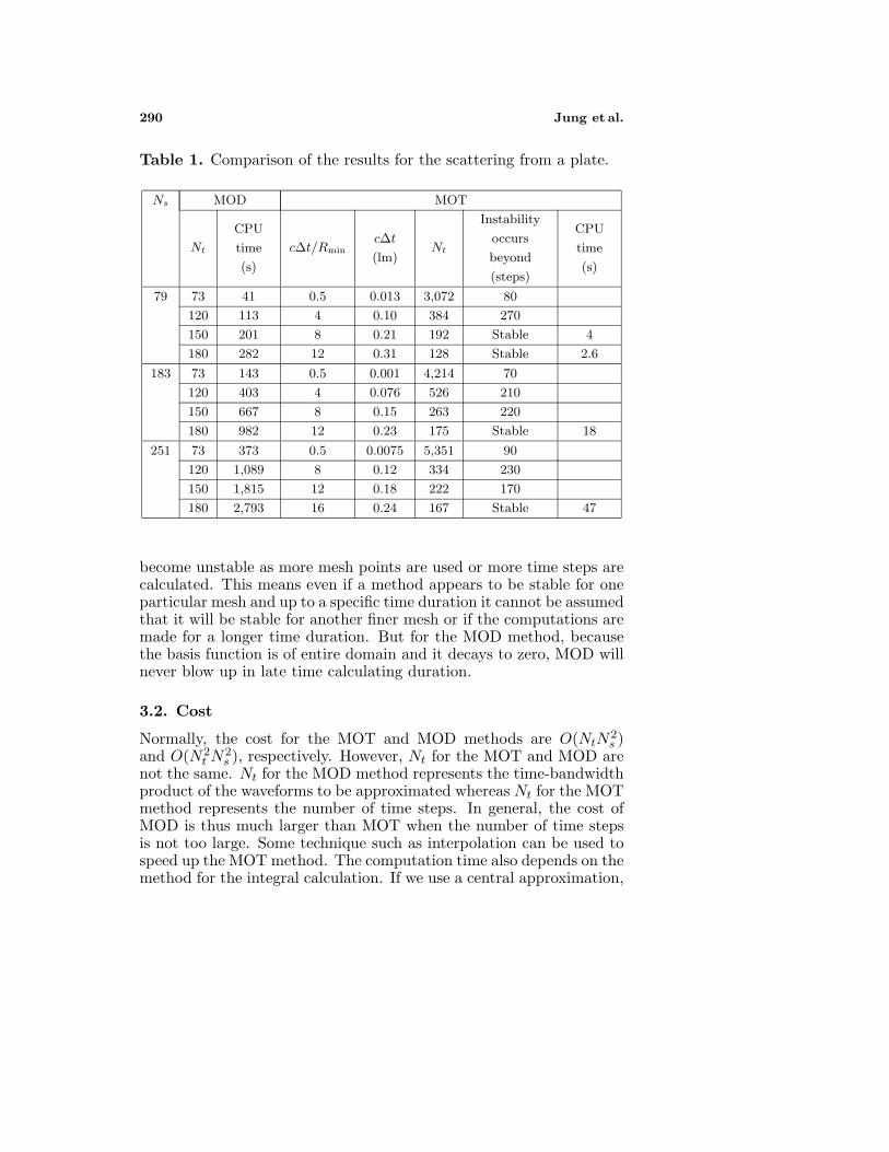
where γ = (4/T ) (ct− ct0 − r · k). T is the width of the pulse andct0 is the time delay at which the pulse reaches its peak. Both ofthese quantities are defined in light meters (lm). In our test examples,T = 4 lm and ct0 = 6 lm. k is the wave vector for the incident wave.Fig. 1(a) shows the induced current at the center of the plate by theMOT and MOD methods with the inverse discrete Fourier transform(IDFT) of the frequency-domain result. In order to see the differenceclearly, Fig. 1(b) shows the enlarged part of it. We compare thestability for different mesh size and different number of temporal basisfunctions both for the MOT and MOD method in Table 1. In Table 1,Rmin is the minimum distance between two nodes of the structure.The results of the MOD method are always stable if Ns is larger thana certain number which depends on the bandwidth of the incidentsignal and duration of the calculation [19].

For the MOT method, the results are often unstable for theexplicit case. For the implicit case, it appears to be stable when acareful choice of the time step is made. It seems in this case the propertime step is around 0.2 ∼ 0.3 lm. When the solution is unstable, theerrors are amplified at each time step. The growth of the error isgoverned by the number of time steps and not by the total time andquickly becomes large enough to swamp the solution. The instabilitycan often be reduced or eliminated for a particular mesh by averagingthe current in time [5, 12] or space [10, 13]. These schemes typically

Progress In Electromagnetics Research, PIER 70, 2007 289

(a)

(b)

Figure 1. Induced current at the center of the plate. (a) Wholeduration, (b) zoom out part of (a).

290 Jung et al.

Table 1. Comparison of the results for the scattering from a plate.

Ns MOD MOT

Nt

CPU

time

(s)

c∆t/Rminc∆t

(lm)Nt

Instability

occurs

beyond

(steps)

CPU

time

(s)

79 73 41 0.5 0.013 3,072 80

120 113 4 0.10 384 270

150 201 8 0.21 192 Stable 4

180 282 12 0.31 128 Stable 2.6

183 73 143 0.5 0.001 4,214 70

120 403 4 0.076 526 210

150 667 8 0.15 263 220

180 982 12 0.23 175 Stable 18

251 73 373 0.5 0.0075 5,351 90

120 1,089 8 0.12 334 230

150 1,815 12 0.18 222 170

180 2,793 16 0.24 167 Stable 47

become unstable as more mesh points are used or more time steps arecalculated. This means even if a method appears to be stable for oneparticular mesh and up to a specific time duration it cannot be assumedthat it will be stable for another finer mesh or if the computations aremade for a longer time duration. But for the MOD method, becausethe basis function is of entire domain and it decays to zero, MOD willnever blow up in late time calculating duration.

3.2. Cost

Normally, the cost for the MOT and MOD methods are O(NtN2s )

and O(N2t N

2s ), respectively. However, Nt for the MOT and MOD are

not the same. Nt for the MOD method represents the time-bandwidthproduct of the waveforms to be approximated whereas Nt for the MOTmethod represents the number of time steps. In general, the cost ofMOD is thus much larger than MOT when the number of time stepsis not too large. Some technique such as interpolation can be used tospeed up the MOT method. The computation time also depends on themethod for the integral calculation. If we use a central approximation,

Progress In Electromagnetics Research, PIER 70, 2007 291

(a)

(b)

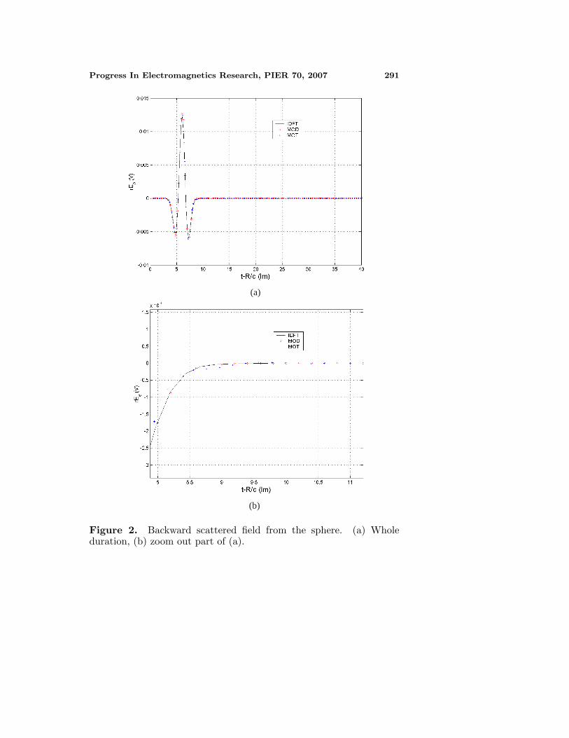
Figure 2. Backward scattered field from the sphere. (a) Wholeduration, (b) zoom out part of (a).

292 Jung et al.

Figure 3. A conducting cone.

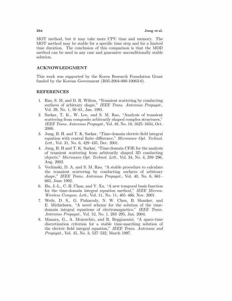
Figure 4. The induced current across edge 67 of the cone.

Progress In Electromagnetics Research, PIER 70, 2007 293

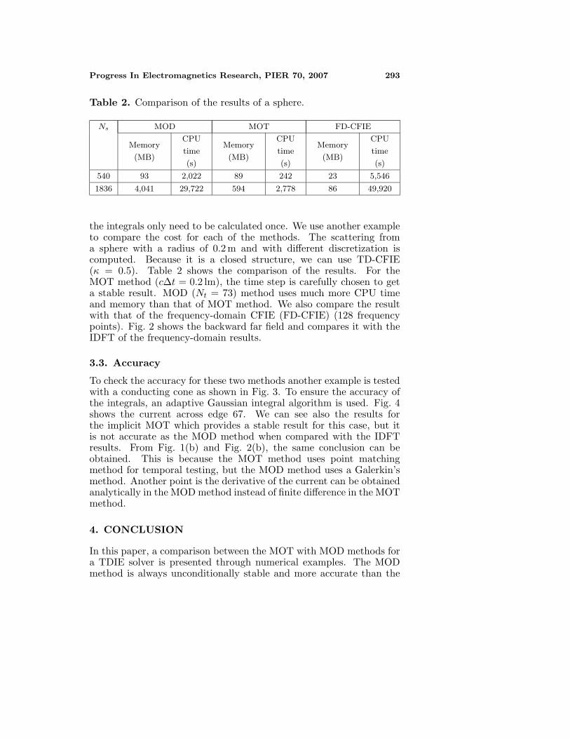
Table 2. Comparison of the results of a sphere.

Ns MOD MOT FD-CFIE

Memory

(MB)

CPU

time

(s)

Memory

(MB)

CPU

time

(s)

Memory

(MB)

CPU

time

(s)

540 93 2,022 89 242 23 5,546

1836 4,041 29,722 594 2,778 86 49,920

the integrals only need to be calculated once. We use another exampleto compare the cost for each of the methods. The scattering froma sphere with a radius of 0.2 m and with different discretization iscomputed. Because it is a closed structure, we can use TD-CFIE(κ = 0.5). Table 2 shows the comparison of the results. For theMOT method (c∆t = 0.2 lm), the time step is carefully chosen to geta stable result. MOD (Nt = 73) method uses much more CPU timeand memory than that of MOT method. We also compare the resultwith that of the frequency-domain CFIE (FD-CFIE) (128 frequencypoints). Fig. 2 shows the backward far field and compares it with theIDFT of the frequency-domain results.

3.3. Accuracy

To check the accuracy for these two methods another example is testedwith a conducting cone as shown in Fig. 3. To ensure the accuracy ofthe integrals, an adaptive Gaussian integral algorithm is used. Fig. 4shows the current across edge 67. We can see also the results forthe implicit MOT which provides a stable result for this case, but itis not accurate as the MOD method when compared with the IDFTresults. From Fig. 1(b) and Fig. 2(b), the same conclusion can beobtained. This is because the MOT method uses point matchingmethod for temporal testing, but the MOD method uses a Galerkin’smethod. Another point is the derivative of the current can be obtainedanalytically in the MOD method instead of finite difference in the MOTmethod.

4. CONCLUSION

In this paper, a comparison between the MOT with MOD methods fora TDIE solver is presented through numerical examples. The MODmethod is always unconditionally stable and more accurate than the

294 Jung et al.

MOT method, but it may take more CPU time and memory. TheMOT method may be stable for a specific time step and for a limitedtime duration. The conclusion of this comparison is that the MODmethod can be used in any case and guarantee unconditionally stablesolution.

ACKNOWLEDGMENT

This work was supported by the Korea Research Foundation Grantfunded by the Korean Government (R05-2004-000-10063-0).

REFERENCES

1. Rao, S. M. and D. R. Wilton, “Transient scattering by conductingsurfaces of arbitrary shape,” IEEE Trans. Antennas Propagat.,Vol. 39, No. 1, 56–61, Jan. 1991.

2. Sarkar, T. K., W. Lee, and S. M. Rao, “Analysis of transientscattering from composite arbitrarily shaped complex structures,”IEEE Trans. Antennas Propagat., Vol. 48, No. 10, 1625–1634, Oct.2000.

3. Jung, B. H. and T. K. Sarkar, “Time-domain electric-field integralequation with central finite difference,” Microwave Opt. Technol.Lett., Vol. 31, No. 6, 429–435, Dec. 2001.

4. Jung, B. H and T. K. Sarkar, “Time-domain CFIE for the analysisof transient scattering from arbitrarily shaped 3D conductingobjects,” Microwave Opt. Technol. Lett., Vol. 34, No. 4, 289–296,Aug. 2002.

5. Vechinski, D. A. and S. M. Rao, “A stable procedure to calculatethe transient scattering by conducting surfaces of arbitraryshape,” IEEE Trans. Antennas Propagat., Vol. 40, No. 6, 661–665, June 1992.

6. Hu, J.-L., C. H. Chan, and Y. Xu, “A new temporal basis functionfor the time-domain integral equation method,” IEEE Microw.Wireless Compon. Lett., Vol. 11, No. 11, 465–466, Nov. 2001.

7. Weile, D. S., G. Pisharody, N. W. Chen, B. Shanker, andE. Michielssen, “A novel scheme for the solution of the time-domain integral equations of electromagnetics,” IEEE Trans.Antennas Propagat., Vol. 52, No. 1, 283–295, Jan. 2004.

8. Manara, G., A. Monorchio, and R. Reggiannini, “A space-timediscretization criterion for a stable time-marching solution ofthe electric field integral equation,” IEEE Trans. Antennas andPropagat., Vol. 45, No. 3, 527–532, March 1997.

Progress In Electromagnetics Research, PIER 70, 2007 295

9. Davies, P. J., “Numerical stability and convergence of approxima-tions of retarded potential integral equations,” SIAM J. Numer.Anal., Vol. 31, 856–875, June 1994.

10. Davies, P. J., “On the stability of time-marching schemes forthe general surface electric-field integral equation,” IEEE Trans.Antennas Propagat., Vol. 44, No. 11, 1467–1473, Nov. 1996.

11. Shankar, B., A. A. Ergin, K. Aygun, and E. Michielssen, “Analysisof transient electromagnetic scattering from closed surfaces usinga combined field integral equation,” IEEE Trans. AntennasPropagat., Vol. 48, No. 7, 1064–1074, July 2000.

12. Rynne, B. P. and P. D. Smith, “Stability of time marchingalgorithms for the electric field equation,” J. Electromagn. WavesApplicat., Vol. 4, 1181–1205, 1990.

13. Davies, P. J., “A stability analysis of a time marching scheme forthe general surface electric field integral equation,” Appl. Nume.Math., Vol. 27, 33–57, 1998.

14. Tijhuis, A. G., “Toward a stable marching-on-in-time method fortwo-dimensional transient electromagnetic scattering problems,”Radio Sci., Vol. 19, 1311–1317, 1984.

15. Sadigh, A. and E. Arvas, “Treating the instabilities in marching-on-in-time method from a different perspective,” IEEE Trans.Antennas Propagat., Vol. 41, No. 12, 1695–1702, Dec. 1993.

16. Yla-Oijala, P., M. Taskiene, and J. Sarvas, “Surface integralequation method for general composite metallic and dielectricstructures with junctions,” Progress In Electromagnetics Research,PIER 52, 81–108, 2005.

17. Hanninen, I., M. Taskinen, and J. Sarvas, “Singularity subtractionintegral formulae for surface integral equations with RWG,rooftop and hybrid basis functions,” Progress In ElectromagneticsResearch, PIER 63, 243–278, 2006.

18. Wang, S., X. Guan, D. Wang, X. Ma, and Y. Su, “Electromagneticscattering by mixed conducting/dielectric objects using higher-order MoM,” Progress In Electromagnetics Research, PIER 66,51–63, 2006.

19. Chung, Y.-S., T. K. Sarkar, and B. H. Jung, “Solution of atime-domain magnetic-field integral equation for arbitrarily closedconducting bodies using an unconditionally stable methodology,”Microwave Opt. Technol. Lett., Vol. 35, No. 6, 493–499, Dec. 2002.

20. Jung, B. H., Y.-S. Chung, and T. K. Sarkar, “Time-domain EFIE,MFIE, and CFIE formulations using Laguerre polynomials astemporal basis functions for the analysis of transient scattering

296 Jung et al.

from arbitrary shaped conducting structures,” Progress InElectromagnetics Research, PIER 39, 1–45, 2003.

21. Jung, B. H., T. K. Sarkar, Y.-S. Chung, M. Salazar-Palma,and Z. Ji, “Time-domain combined field integral equation usingLaguerre polynomials as temporal basis functions,” Int. J. Nume.Model., Vol. 17, No. 3, 251–268, 2004.

22. Jung, B. H., T. K. Sarkar, and M. Salazar-Palma, “Timedomain EFIE and MFIE formulations for analysis of transientelectromagnetic scattering from 3-D dielectric objects,” ProgressIn Electromagnetics Research, PIER 39, 113–142, 2004.

23. Jung, B. H., T. K. Sarkar, and Y.-S. Chung, “Solution oftime domain PMCHW formulation for transient electromagneticscattering from arbitrarily shaped 3-D dielectric objects,” ProgressIn Electromagnetics Research, PIER 45, 291–312, 2004.

24. Poularikas, A. D., The Transforms and Applications Handbook,IEEE Press, 1996.

25. Gradshteyn, I. S. and I. M. Ryzhik, Table of Integrals, Series, andProducts, Academic Press, New York, 1980.

26. Rao, S. M., D. R. Wilton, and A. W. Glisson, “Electromagneticscattering by surfaces of arbitrary shape,” IEEE Trans. AntennasPropagat., Vol. 30, No. 3, 409–418, May 1982.