A COMPARISON OF MAGNETOELECTRIC TRANSDUCER

DESIGNS FOR USE AS WIRELESS MAGNETIC POWER

RECEIVERS IN BIOMEDICAL IMPLANT APPLICATIONS

by

Tyrel Rupp

A thesis submitted to the faculty of The University of Utah

in partial fulfillment of the requirements for the degree of

Master of Science

Department of Mechanical Engineering

The University of Utah

May 2018

Copyright © Tyrel Christian Rupp 2018

All Rights Reserved

T h e U n i v e r s i t y o f U t a h G r a d u a t e S c h o o l

STATEMENT OF THESIS APPROVAL

The thesis of Tyrel Christian Rupp

has been approved by the following supervisory committee members:

Shad J. Roundy , Chair

Date Approved

Hanseup Kim , Member

Date Approved

Jiyoung Chang , Member

Date Approved

and by Tim Ameel , Chair of

the Department of Mechanical Engineering

and by David B. Kieda, Dean of The Graduate School.

iii

ABSTRACT

Inherent in the nature of medical implant designs is the need to minimize their

size and subsequent impact to their environment of use. Recently, many of the

mechanisms used in implants have been constructed on the micro and even nano scales,

however powering these devices still remains a challenge. One of the more elegant

solutions to this issue would be to construct a microscale wireless power receiver (or

transducer) to deliver the needed power. This work serves to compare the viability of two

transducer designs as candidates for their use as such a receiver.

In particular the designs both use alternating magnetic fields as the power

transmission medium and mechanically couple the magnetic and electric domains. The

first design is a longitudinal (extension) mode magnetoelectric laminate comprised of

magnetostrictive and piezoelectric layers. The second design is a symmetrically built

mechano-magneto-electric transducer consisting of a piezoelectric bimorph with a

permanent magnet mounted at its tip.

A lumped parameter model was developed for the bending design while an

existing model of the longitudinal design was augmented so that the power output of each

device could be predicted and compared. Additionally, these models were experimentally

validated. A linear numerical optimization was then performed using the models. The

optimization was constrained at 2 mm3 maximum size as well as by IEEE and ICNIRP

field restrictions to reflect the requirements of a medical implant.

The results of the optimization showed that a magnetoelectric laminate made of

Metglas and PZT layers delivered more power than that of a symmetric mechano-

magnetoelectric transducer made of Brass, PZT and Neodymium. Under IEEE field

restrictions this amounted to ~40 mW of power delivery compared to ~4 mW. Under the

ICNIRP restrictions the corresponding power outputs are ~60 µW and ~26 µW

respectively. These results indicate that a magnetoelectric laminate, particularly under

IEEE conditions, is the more feasible of the two designs for powering microscale

implants and efforts should be made to develop such a transducer.

v

This thesis is dedicated to Gloria Rupp for teaching me to love learning, to Wally Rupp for instilling in me the importance of hard work, and ultimately to the both of them for

demonstrating to me what can come when these two passions are combined.

vi

TABLE OF CONTENTS

ABSTRACT ...................................................................................................................... iii

LIST OF TABLES .......................................................................................................... viii

LIST OF FIGURES .......................................................................................................... ix

LIST OF SYMBOLS AND ABBREVIATIONS ............................................................. xi

ACKNOWLEDGMENTS .............................................................................................. xvi

1. INTRODUCTION .......................................................................................................... 1

1.1 Project Motivation ............................................................................................... 2 1.2 Project Goals ........................................................................................................ 3

2. A REVIEW OF MAGNETOELECTRIC TRANSDUCERS AND THEIR WPT APPLICATIONS ................................................................................................................ 4

2.1 Non Magnetoelectric based Wireless Power Transfer Systems .......................... 4 2.1.1 Inductive Coupling based WPT ............................................................... 5 2.1.2 Acoustic based WPT ................................................................................ 5 2.1.3 Radio Frequency based WPT................................................................... 6

2.2 Development of the Magnetoelectric Effect ........................................................ 6 2.2.1 History of Magnetoelectric Composites .................................................. 7 2.2.2 Development of Magnetostrictive Materials ........................................... 8

2.3 Review of Magnetoelectric Laminate Work ........................................................ 9 2.3.1 Magnetoelectric Bimorph Designs ........................................................ 10

2.4 Mechano-Magnetoelectric Design ..................................................................... 11 2.5 Current applications of ME transducers ............................................................ 12

2.5.1 ME Applications: Sensors and other electronic devices ........................ 12 2.5.2 ME Applications: Medical uses ............................................................. 12

3. LUMPED ELEMENT MODELS FOR MAGNETOSTRICTIVE AND DOUBLE CANTELEVER TRANSDUCERS .................................................................................. 14

3.1 Lumped Parameter Power Model for ME bimorph ........................................... 14 3.1.1 Summary of the ME bimorph voltage model by Dong Et Al. ............... 15 3.1.2 Limitations of Dong et al. model ........................................................... 19 3.1.3 ME Laminate Model for Power Delivery Prediction ............................. 22 3.1.4 Longitudinal-Transverse Model Augmentation ..................................... 24

3.2 Lumped Parameter Model for MME “Butterfly” Transducer ........................... 27 3.2.1 MME Geometry and Model Summary .................................................. 27 3.2.2 Limitations of the MME transducer model ............................................ 30

4. EXPERIMENTAL VALIDATION OF TRANSDUCER MODELS ........................... 34

4.1 Experimental Setup ............................................................................................ 34 4.1.1 Nested Helmholtz Coil Design .............................................................. 35 4.1.2 Nested Helmholtz Coil Performance ..................................................... 36 4.1.3 Additional DC Field Biasing Measures ................................................. 38

4.2 Fabrication of ME Transducers ......................................................................... 39 4.2.1 Galfenol-PZT Transducer ...................................................................... 39 4.2.2 Metglas-PVDF transducer ..................................................................... 40

4.3 Galfenol-PZT Device Characterization and Model Comparison ....................... 42 4.3.1 Optimal Bias Field ................................................................................. 42 4.3.2 Open Circuit Voltage Testing ................................................................ 43 4.3.3 Tuned Comparison Model ..................................................................... 45 4.3.4 Optimal Load and Power Delivery ........................................................ 46

4.4 Metglas-PVDF Device Characterization and Model Comparison ..................... 49 4.4.1 Open Circuit Voltage Testing and Tuned Model ................................... 50 4.4.2 Optimal Load and Power Delivery ........................................................ 52

4.5 MME Model Validation ..................................................................................... 54

5. COMPARATIVE ANALYSIS OF TRANSDUCER TYPES ...................................... 56

5.1 Optimization Algorithm ..................................................................................... 56 5.2 Optimization Constraints and Bounds ............................................................... 57

5.2.1 ME Transducer Optimization Constraints ............................................. 59 5.2.2 MME Transducer Optimization Constraints .......................................... 61

5.3 ME Optimization and Results ............................................................................ 62 5.3.1 Discussion of ME Optimization Results ................................................ 64

5.4 MME Optimization and Results ........................................................................ 66 5.4.1 Discussion of MME Optimization Results ............................................ 71

5.5 Comparison of Optimized Structures ................................................................. 73

6. FUTURE WORK AND CONCLUSIONS ................................................................... 75

6.1 Conclusions ........................................................................................................ 75 6.2 Future Work ....................................................................................................... 77

REFERENCES ................................................................................................................ 79

viii

LIST OF TABLES

Tables Table 3.1: Lumped parameter equations for L-L ME laminate. ....................................... 19

Table 3.2: Corrected lumped parameters for L-T configuration. ...................................... 26

Table 3.3: Lumped parameters for MME transducer. ....................................................... 32

Table 4.1: Nested Helmholtz Coil geometry.. .................................................................. 35

Table 4.2: Built nested Helmholtz Coil performance and predictions.. ............................ 37

Table 4.3: Material properties used for Galfenol-PZT laminate model. ........................... 46

Table 4.4: Material properties used for Metglas-PVDF model. ....................................... 51

Table 5.1: ME optimization results. .................................................................................. 63

Table 5.2: Neodymium 52 material properties. ................................................................ 67

Table 5.3: MME optimization results for 10 mm and 5 mm magnet. .............................. 69

Table 5.4: Final MME optimization results. ..................................................................... 70

Table 5.4: Power outputs of MME and ME transducers compared. ................................. 74

ix

LIST OF FIGURES

Figures

Figure 2.1: Magnetoelectric structure layout similar to that made by Shin et al. ............... 8

Figure 2.2: Four bimorph laminate orientation combinations. ......................................... 10

Figure 3.1: Geometry layout for L-L mode bimorph. ....................................................... 15

Figure 3.2: Lumped element equivalent circuit of L-L ME laminate. .............................. 16

Table 3.1: Lumped parameter equations for L-L ME laminate. ....................................... 19

Figure 3.3: A typical magnetostriction profile and its derivative. .................................... 21

Figure 3.4: Magnetoelectric equivalent circuit with added load resistor. ......................... 23

Figure 3.5: Geometry layout for L-T mode bimorph. ....................................................... 26

Figure 3.6: Geometry layout for the double cantilever MME structure. .......................... 28

Figure 3.7: Lumped element equivalent circuit of double cantilever MME structure ...... 28

Figure 4.1: Magnetoelectric transducer experimental test setup diagram. ....................... 35

Figure 4.2: Nested Helmholtz Coil built for experimental validation. ............................. 36

Figure 4.3: Biasing magnet arrangement and resulting field lines. .................................. 39

Figure 4.4: Galfenol-PZT ME transducer, shown anchored at its center (left), and zoomed in on the cross section (right). ........................................................................................... 40

Figure 4.5: Metglas-PVDF ME transducer with bonded leads visible. ............................ 41

Figure 4.6: Galfenol-PZT structure mounted in bias field stage. ..................................... 43

Figure 4.7: Repeated open circuit voltage vs frequency. .................................................. 45

Figure 4.8: Power output vs load resistance for Galfenol-PZT device operating at 71 kHz............................................................................................................................................ 47

Figure 4.9 Power output vs frequency for the Galfenol-PZT device loaded at 2.3kΩ. .... 48

Figure 4.10: Metglas-PVDF Transducer as mounted, shown from the side and top. ....... 50

Figure 4.11: Metglas-PVDF open circuit voltage versus frequency................................. 51

Figure 4.12: Power output vs load resistance for Metglas-PVDF device operating at natural frequency .............................................................................................................. 52

Figure 4.13: Power output vs frequency for the Metglas-PVDF device loaded at 1.9kΩ 53

Figure 4.14: Experimental and modeled MME transducer power output across frequency............................................................................................................................................ 55

Figure 4.15: Experimental and modeled MME transducer power output under varying B-field at 350 Hz operating frequency. ................................................................................. 55

Figure 5.1: Magnetic MPE levels for IEEE and ICNIRP Standards. ............................... 58

Figure 5.2: Normal strain gradients for right hand side of an ME device. ....................... 60

Figure 5.3: Average FEM strain, normalized by perfect the strain assumption, vs l0/tt ratio. .................................................................................................................................. 61

Figure 5.4: CAD representation optimized Metglas-PZT device under IEEE safety conditions. ......................................................................................................................... 64

Figure 5.5: CAD representation optimized PZT-Brass-N52 device constrained to 1 mm magnet height. ................................................................................................................... 71

xi

LIST OF SYMBOLS AND ABBREVIATIONS

FEM Finite element model

ICNIRP International Commission on Non-Ionizing Radiation Protection

IEEE Institute of Electrical and Electronics Engineers

IMD Implantable medical device

ME Magnetoelectric

MME Mechano-magnetoelectric

MS Magnetostrictive

MPE Maximum Permissible Exposure

PE Piezoelectric

PM Piezomagnetic

PVDF Polyvinylidene fluoride

PZT Lead zirconate titanate

RF Radio frequency

WPT Wireless power transfer

L-L Longitudinal-Longitudinal

L-T Longitudinal-Transverse

T-L Transverse-Longitudinal

T-T Transverse-Transvers

𝐴𝐴1 Total piezoelectric cross-sectional area

𝐴𝐴2 Total magnetostrictive cross-sectional area

xii

αME Magnetoelectric coefficient

𝑏𝑏 Damping coefficient

𝛽𝛽𝑝𝑝 Inverse dielectric constant of piezoelectric material

𝛽𝑝𝑝 Effective inverse dielectric constant of piezoelectric material

𝐶𝐶0 Clamped piezo electric capacitance

𝐶𝐶𝑚𝑚 Mechanical capacitance or compliance

𝑑𝑑33,𝑚𝑚 Piezomagnetic material coefficient (parallel to field)

𝜖𝜖0 Vacuum permittivity

𝑒𝑒33 Effective piezoelectric stress constant

𝐸𝐸𝑃𝑃 Piezoelectric modulus of elasticity

𝐸𝐸𝑠𝑠 Substrate modulus of elasticity

(𝐸𝐸𝐸𝐸)𝑐𝑐 Composite flexural rigidity

𝑓𝑓(𝑥𝑥) Objective Function

𝐹𝐹𝑚𝑚 Equivalent force due to magnet moment

𝑔𝑔33,𝑝𝑝 Piezoelectric voltage coefficient (parallel to poling) 𝑔𝑔31,𝑝𝑝 Piezoelectric voltage coefficient (perpendicular to poling)

ℎ Magnet height

𝐻𝐻 Magnetic field strength

𝐻𝐻𝑝𝑝 Sinusoidal magnetic field magnitude

𝐻𝐻𝐷𝐷𝐷𝐷 Continuous (DC) magnetic field magnitude

𝐽𝐽𝑟𝑟 Remnant magnetic polarization

𝐾𝐾3𝑇𝑇 Relative dielectric constant

𝐾𝐾0 Short-circuit stiffness

xiii

𝐾𝐾1 Optimal load stiffness

∆𝐾𝐾 Change in stiffness due to loading

𝑙𝑙 Laminate length

𝑙𝑙𝑒𝑒𝑒𝑒𝑒𝑒 Effective beam length

𝑙𝑙0 Length from anchor to free edge

𝐿𝐿 Beam length

𝐿𝐿0 Beam length to magnet

𝐿𝐿𝑚𝑚 Magnet length

𝐿𝐿𝑚𝑚 Mechanical inductance or inertia

𝑀𝑀 Magnet mass

𝑚𝑚 Effective mass

𝑚𝑚𝑏𝑏 Beam mass

𝑀𝑀𝑏𝑏 Moment due to magnet

𝑀𝑀1 Variable used for simplification

𝜆𝜆 Magnetostriction constant

𝑛𝑛 Volumetric layer ratio

𝜔𝜔 Operating frequency

𝜔𝜔𝑠𝑠 Fundamental/natural frequency

𝜔𝜔1 Loaded natural frequency

𝑃𝑃 Power output

𝑃𝑃𝑝𝑝 Peak power output

𝑃𝑃𝐴𝐴𝐴𝐴𝐴𝐴 Average power output (from RMS voltage)

𝑃𝑃𝐴𝐴𝐴𝐴𝐴𝐴𝑜𝑜𝑝𝑝𝑜𝑜 Optimal average power

xiv

𝜑𝜑𝑚𝑚 Magnetoelectric coupling coefficient

𝜑𝜑𝑝𝑝 Piezoelectric coupling factor

𝑄𝑄𝑚𝑚 Effective laminate quality factor

𝑄𝑄𝑝𝑝 Power output quality factor

𝑄𝑄𝑚𝑚𝑠𝑠 Magnetostrictive quality factor

𝑄𝑄𝑝𝑝𝑒𝑒 Piezoelectric quality factor

𝜌𝜌𝑎𝑎𝑎𝑎𝑎𝑎 Average laminate density

𝜌𝜌𝑀𝑀 Magnet density

𝜌𝜌𝑚𝑚𝑠𝑠 Magnetostrictive material density

𝜌𝜌𝑝𝑝𝑒𝑒 Piezoelectric material density

𝜌𝜌𝑠𝑠 Substrate density

𝑠𝑠33𝐻𝐻 Elastic compliance of the MS material (parallel to field)

𝑠𝑠33𝐷𝐷 Elastic compliance of the PE material (parallel to poling)

𝑠𝑠11𝐷𝐷 Elastic compliance of the PE material (perpendicular to poling)

Ssub Structural interface layer

𝜎𝜎𝑇𝑇 Max tensile stress

𝜎𝜎𝐵𝐵 Max bending stress

𝑡𝑡𝑝𝑝 Piezoelectric layer thickness

𝑡𝑡𝑚𝑚 Magnetostrictive layer thickness

𝑡𝑡𝑠𝑠 Substrate thickness

𝑡𝑡𝑜𝑜 Total Beam/Laminate Thickness

𝜏𝜏 Time constant

𝑣𝑣 Magnetoelectric wave speed

xv

𝑉𝑉𝑚𝑚 Magnet volume

𝑉𝑉𝑂𝑂𝑂𝑂𝑀𝑀𝑂𝑂 Open circuit transducer Voltage (RMS)

𝑉𝑉𝑠𝑠 Substrate volume

𝑉𝑉𝑃𝑃𝑃𝑃 Piezoelectric volume

𝑤𝑤 Beam/laminate width

𝑥𝑥 Input parameters

𝑥𝑥0 Initial guess

𝑋𝑋0 Variable used for simplification

𝑍𝑍0 Characteristic mechanical impedance

𝑍𝑍𝑚𝑚 Mechanical impedance or damping

xvi

ACKNOWLEDGMENTS

I would like to thank all those who have helped make thesis come to reality.

Firstly, gratitude goes to Binh Duc Truong for the contribution of his model as a foundation

to this work. Next, I would like to thank my committee members Hanseup Kim and Jiyoung

Chang for their guidance during my time at the University of Utah. I would also like to thank

the National Science Foundation for funding this project. Great appreciation also goes to all

members of the Integrated Self-powered Sensing Laboratory for their contributions and

friendship. Finally, greatest thanks go to my advisor and committee chair, Dr. Shad Roundy,

for his extreme patience, guidance, and contributions throughout this project and my graduate

school experience.

CHAPTER 1

INTRODUCTION

The continuous improvement of Implantable Medical Devices (IMD) is driven

largely by their proven usefulness in monitoring and augmenting the environment found

within the human body. In the case of Type 1 diabetic patients, the ability to continuously

monitor blood glucose levels provided by implanted probes has been shown to reduce

time spent in hypoglycemia [1]. This mitigation of a potentially fatal condition common

to diabetics is just one of many success stories for IMDs. Beyond real time monitoring,

the ability to deliver targeted drug doses and treat neural disorders via neural prostheses

are just a few of the treatment methods becoming more viable as implants continue to

develop [2], [3]. Utilizing the same technology that brought about micro scale

semiconductors, microfabrication techniques have been used to develop a wide array of

micro sized architectures that could be tremendously useful as implants to the human

body [4]. Along with the reduction in size of the operating mechanisms, significant effort

has also been put into miniaturizing circuitry required to operate them [5]. As it stands,

the limitation behind implementing these microsystems as IMDs is not so much the size

of the sensing mechanism or its circuitry, but rather the size of system used to power it.

To make microscale IMDs more viable, microscale power systems need to be developed.

2

1.1 Project Motivation

Currently the most common way to power IMDs is via a direct (wired) external

source or a battery implanted along with the IMD. Another proposed method is to utilize

a wireless power transfer (WPT) system that can pass power through flesh and bone to

the interior of the human body. Direct power delivery is typically avoided where possible

due to the limitations it causes in patient mobility as well as the increased medical risks

associated with passing wires transcutaneously to the location of the implant. Batteries

help mitigate the problems presented by the direct powering method, however they also

come with their own pitfalls. In the best of cases, batteries have finite lifetimes and

require periodic replacement. More commonly however, in terms of microscale systems,

the sheer size of the batteries alone nullifies the gains made by miniaturizing the other

components of an IMD.

In light of the concerns with the two previously discussed methods, a WPT

system would appear to be the obvious solution but is not without its own set of

difficulties. Acoustic WPT systems have been investigated, but are complicated by the

inability to transmit through bone and the need for direct skin contact [6]. Similarly,

Radio frequency (RF) methods are viable for larger applications, however as RF

receivers are miniaturized their operating frequencies are driven to levels where tissue

tends to absorb and attenuate the transmitted signal [7]. This attenuation is not only

inefficient, it is potentially hazardous because of associated tissue heating. In light of

these difficulties, it rapidly becomes apparent that further research into WPT systems is

required to more fully tailor them to the constraints posed by the human body.

3

1.2 Project Goals

With the need for an improved WPT method for use in microscale IMDs

demonstrated, the goal of this project is to evaluate the practicality of two magnetic field

based methods of WPT as alternatives to RF, acoustic, and inductive coupling methods

applied at microscale sizes. In particular these methods look at two different types of

receiver structure designs, a magneto-electric laminate (ME) extensional mode transducer

and a Mechano-Magneto-Electric (MME) bending mode transducer.

This goal will be accomplished by first experimentally validating two lumped

parameter models representative of the structures in question with macro scale

transducers. Next both models will be used to yield geometries optimized for maximum

power output at microscale sizes. The optimization will be driven by both microscale

manufacturing constraints as well as biological constraints.

Ultimately the main contribution of this project is to use macro sized structures

and modeling to identify which of the two methods (ME or MME) is superior for use at

microscale levels, long before any costly microfabrication has to be performed.

CHAPTER 2

A REVIEW OF MAGNETOELECTRIC TRANSDUCERS AND THEIR WPT

APPLICATIONS

As early as the year 1900, Nikola Tesla was patenting technology related to

wireless energy transfer, and by 1905 he was convinced of its potential to revolutionize

the world [8], [9]. This effort demonstrated the model for all future wireless energy

transfer research by showing the need for both a transmitter to send the power and a

receiver to capture the power. Despite Tesla’s enthusiasm, for many years research into

wirelessly powering devices was largely dwarfed by research on wireless

communication. In the case of transcutaneous wireless power transfer, the topic did not

become active until the 1960’s and even then was sparse for the next two decades [10].

Finally, the suggestion to use magnetoelectric (ME) transducers to power IMDs only has

only come in the last two decades as feasibility of ME laminates for WPT has been

shown [11].

2.1 Non Magnetoelectric based Wireless Power Transfer Systems

As was indicated previously, WPT research has typically been based around

structures that employ either magnetic, RF, acoustic, or inductive coupling techniques. It

should be noted that the research at hand focuses mainly on magnetic techniques.

Correspondingly, a detailed literature review of the other three techniques was considered

5

to be superfluous. Rather, the rest of section 2.1 is a brief summary of how these

methods compare when applied to IMDs. In terms of content, unless otherwise cited, this

summary comes from an extensive review performed by Basaeri et al. [12].

2.1.1 Inductive Coupling based WPT

In terms of actually implementing WPT systems to power implants, those

utilizing inductive coupling appear to be the most advanced, principally in the case of

powering pacemakers. Recently Abiri et al. demonstrated functionality of a porcine

implanted, commercial pacemaker (St. Jude Tendril SDX Model 1388T) powered

wirelessly by an ex vivo inductively coupled system [13]. Fundamentally, inductive

coupling utilizes a pair of coils or antennas which must be closely and well aligned to

allow for the transfer of power. Subsequently the amount power transfer is highly

dependent on the size, orientation, operating frequency of, and distance between the

antennas [14]. Ultimately these dependencies make this form of WPT most viable for

IMDs (such as a pacemaker) where the depth of the implant is relatively shallow and the

alignment of the coils can be well controlled.

2.1.2 Acoustic based WPT

Acoustic WPT, like inductive power transfer, is very alignment dependent in that

the receiver must be well aligned (i.e. precise depth and orientation) to adequately receive

the ultrasound signals being transmitted. Furthermore, to send useful amounts of power,

the transmission medium, typically water or tissue, needs to be consistent. Air gaps or

solids such as bone quickly attenuate the transmission signal. In terms of implementation,

acoustic transducer research hasn’t gone much beyond porcine tissue experiments [15].

6

Nevertheless, given the ability to be implanted deeper and operate at much lower

frequencies than RF and inductive systems, acoustic WPT shows promise, notably for

powering IMDs located abdominally.

2.1.3 Radio Frequency based WPT

Radio frequency based WPT systems, like the others discussed, have both pros

and cons. Unlike acoustic and inductively coupled systems, alignment is not as critical

because receivers do not need to be coupled to the transmitter. However, concerns arise

with RF receivers as their size decreases. As receivers are miniaturized, efficiency drops

precipitously and reduced antenna sizes lead to high operating frequencies. This leads to

transmitters having to operate at levels of electromagnetic radiation that area considered

dangerous for humans due to induced tissue heating. Just the same, research to mitigate

these effects continues undeterred, as demonstrated by the recently designed RF-powered

microscale neural implant radio built by Rajavi et al. [16].

2.2 Development of the Magnetoelectric Effect

The magnetoelectric (ME) effect fundamentally refers to any type of coupling

between electric and magnetic fields found in matter [17]. The first work with such an

effect was done by Röntgen in 1888 when he showed theoretically that by moving a

dielectric material through an electric field it would become magnetized [18]. That same

effect was not confirmed experimentally until 1960 when Dzyaloshinskii witnessed it in

Cr2O3. Despite this breakthrough, subsequent research showed that at best the magneto

electric coefficient (αME) for bulk materials such as Cr2O3 was very low, on the order of

7

100 mV/(cm·Oe) [19]. This along with other various complications, kept the materials

from of much use in practical applications [17].

2.2.1 History of Magnetoelectric Composites

Before the ME effect was even observed in bulk materials, Tellegen suggested

developing composites that demonstrated a cumulative ME effect [20]. The implication

here is that by coupling two separate physical effects (piezoelectric (PE) and

magnetostrictive (MS)) in two separate materials an equivalent ME effect could be

obtained.

The more commonly utilized piezoelectric effect is witnessed in materials that

couple mechanical strain to an induced electric field. Similarly, the magnetostrictive

effect found in some materials couples mechanical strain to an induced magnetic field.

By linking two such materials mechanically, the resulting pseudo ME effect can be

demonstrated simply as [21]

ME Effect = electrical

mechanical ×

mechanicalmagnetic

(2.1)

where the mechanical components in essence cancel out. For almost three decades

attempts to form such a composite involved variations on sintering together small grain

or particulate mixtures of both types of materials, however none of these composites were

shown to have ME coefficients much larger than those found in bulk ME materials [17].

In 1998 Shin et al. bypassed particulate composites and attempted a three-layer

laminate composite approach where the MS material was sputtered as a thin film onto a

8

glass substrate which was then bonded onto a PE base. This design has become known in

the literature as a unimorph and is shown in Figure 2.1. By applying a voltage to the PE,

the bending strain induced into the MS material caused large changes to its magnetic

properties [22].

Figure 2.1: Magnetoelectric structure layout similar to that made by Shin et al. The MS material is and orientation is shown in orange, the PE material in blue, and the glass is in-between.

Building on the ME laminate approach taken by Shin et al., Ryu et al. developed

another ME laminate using a sandwich design. This design used silver epoxy to bond a

PZT-5A PE disk between two Terfenol-D MS disks. Measuring the αME under various

magnetic field strengths yielded values up to 4.68 V/(cm·Oe) [23]. Not only was this an

overwhelming improvement to the mV/(cm·Oe) level previously reported for particulate

based ME composites, it brought the ME effect to a point of usefulness.

2.2.2 Development of Magnetostrictive Materials

Just as critical to ME laminate development was the materials involved. The work

done by Ryu et al. relied upon a material, as indicated previously, known by the trade

name “Terfenol-D.” As a rare earth alloy composed of Terbium, Dysprosium, and Iron,

Terfenol-D is a direct product of extensive research done by the U.S. navy in the 1960s to

find a material with what is now known as a “giant” magnetostrictive effect when placed

9

in a magnetic fields [24]. Terfenol has a saturation microstrain of 2500 ppm (µm/m). By

comparison, cobalt and nickel have the largest known bulk material saturation

microstrain on the order of 10 ppm, hence the term “giant” [25].

In the late 90s the U.S. Navy also discovered that Galfenol, an iron-gallium alloy,

had high magnetostriction[26]. With a maximum saturation strain of 400 ppm, Galfenol

is an attractive alternate to Terfenol-D because it costs about 80% less to manufacture

and is significantly easier to machine[27]. A final MS material that should be mentioned

and will be discussed more rigorously later in the body of this thesis is an amorphous

metal known by its trade name as METGLAS (2605SA1). Although it does not have an

exceptionally high maximum MS saturation strain (23 ppm), its high magnetic

permeability allows for the maximum saturation to occur at much lower magnetic fields

than most any other MS material[28], [29].

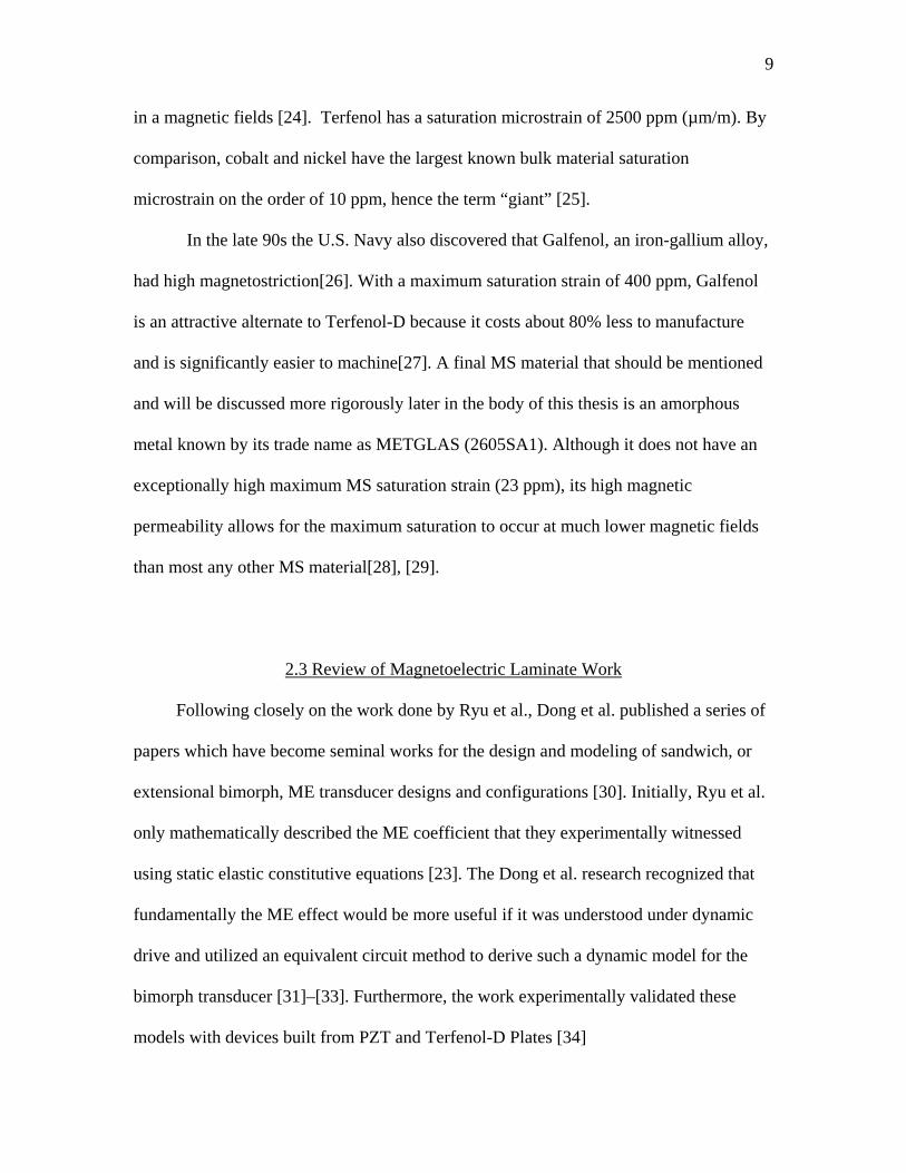
2.3 Review of Magnetoelectric Laminate Work

Following closely on the work done by Ryu et al., Dong et al. published a series of

papers which have become seminal works for the design and modeling of sandwich, or

extensional bimorph, ME transducer designs and configurations [30]. Initially, Ryu et al.

only mathematically described the ME coefficient that they experimentally witnessed

using static elastic constitutive equations [23]. The Dong et al. research recognized that

fundamentally the ME effect would be more useful if it was understood under dynamic

drive and utilized an equivalent circuit method to derive such a dynamic model for the

bimorph transducer [31]–[33]. Furthermore, the work experimentally validated these

models with devices built from PZT and Terfenol-D Plates [34]

10

2.3.1 Magnetoelectric Bimorph Designs

More explicitly, their work created model subsets for each of the four coupling

orientation combinations possible for the PE and MS materials within the laminate

structure. These configurations are compiled and shown in Figure 2.2 and indicate

whether the PE and MS materials are poled longitudinally or transversely to the bimorph

structure.

Figure 2.2: Four bimorph laminate orientation combinations. Orange indicates MS material, blue the PE material, and black the location of the PE poles. Additionally, the letters in the mode names, T for transverse and L for longitudinal, indicate the orientation of the MS material and PE material respectively. Compiled from [31]–[34].

11

Although a tremendous amount of work has gone into the extensional mode

bimorph structures, many other laminate designs have been considered, not the least of

which is the unimorph design that was used originally by [22]. Unlike the bimorph, the

unimorph design is not a symmetric laminate which means that its first mode shape under

magnetic drive is in bending rather than extension. This has been argued to be

advantageous in that it has a lower natural frequency than the bimorph, however it

remains for the efficiency of the two structure designs to be critically compared [30].

Beside the unimorph, a whole variety of other exotic designs exist or have been

proposed for pseudo ME transducers. For the sake of this research most of the geometries

add a level of complexity that is both prohibitive for modeling as well as manufacturing

at the microscale [35]. However, there is one final design that requires mentioning.

2.4 Mechano-Magnetoelectric Design

Fundamentally, a magnetoelectric transducer is any device that takes energy from

the magnetic domain to the electric domain and vice versa. Up to this point the

transducers previously discussed fall into this category, as well as the category of pseudo

ME material since they can be altered like a bulk material and still maintain their ME

properties.

Recently another type of ME transducer, that is fundamentally not a pseudo ME

material, has been proposed. This transducer operates by coupling the moment induced

on ferromagnet by a magnetic field with a bending or cantilever PE beam. This is done

by anchoring one end of the beam and by mounting the ferromagnet at the tip of the beam

oriented perpendicular to the field [36]. To this point, the research done on such a device

12

has been for the purpose of energy scavenging and the corresponding models are found to

be lacking. Nevertheless the design shows significant promise for WPT [36], [37].

Although fundamentally using the same designs of interest, publications have yet to

use a consistent name for this geometry. As it such will be referred to in this work simply

as a Mechano-Magnetoelectric or MME device.

2.5 Current applications of ME transducers

Originally the motivation behind the U.S. Navy to develop MS materials was for

the use in sonar systems, however the progress made has ME applications a growing field

of research [24].

2.5.1 ME Applications: Sensors and other electronic devices

The most notable application for magnetoelectric composites is in sensing AC and

DC magnetic fields and for current sensing. Multiple designs have been suggested,

demonstrated, and even patented that use thin film ME composites at micro and

nanoscales [38], [39]. These designs are particularly useful for their extremely high

sensitivities to changes in magnetic fields [40], [41]. In addition to sensing, there are also

applications for ME composites as gyrators and transformers in microwave devices and

as microactuators[42].

2.5.2 ME Applications: Medical uses

O’Handley et al. first suggested utilizing a ME bimorph for transcutaneous power

transfer in 2008. Additionally, their research showed that in air a .1 cm3 receiver could

generate 2 mW at a distance of 3 cm from a transmitting solenoid[11]. Citing O’Handley

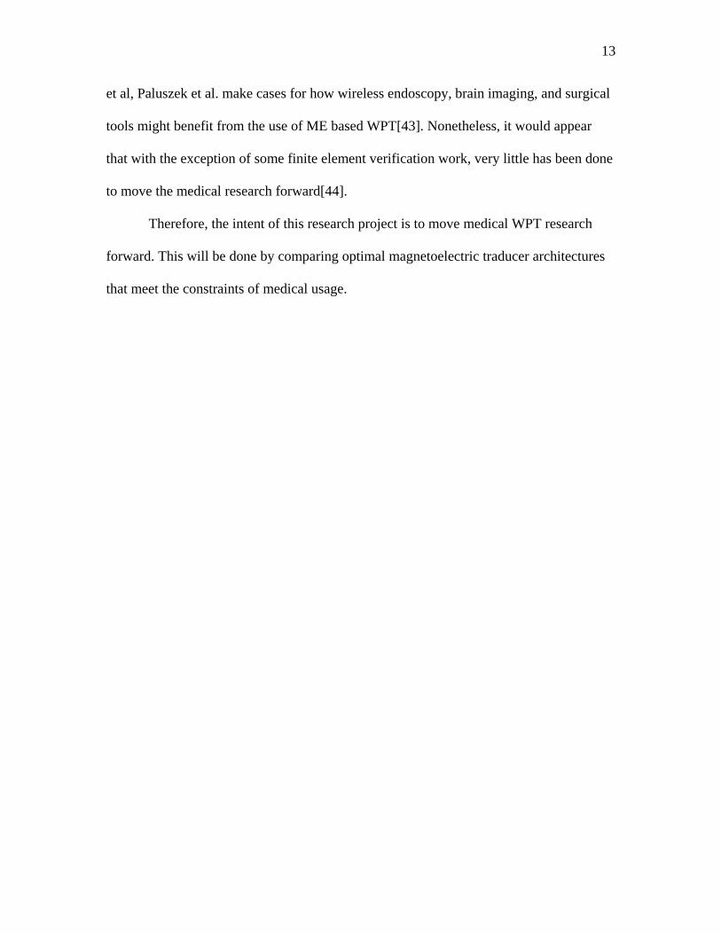
13

et al, Paluszek et al. make cases for how wireless endoscopy, brain imaging, and surgical

tools might benefit from the use of ME based WPT[43]. Nonetheless, it would appear

that with the exception of some finite element verification work, very little has been done

to move the medical research forward[44].

Therefore, the intent of this research project is to move medical WPT research

forward. This will be done by comparing optimal magnetoelectric traducer architectures

that meet the constraints of medical usage.

CHAPTER 3

LUMPED ELEMENT MODELS FOR MAGNETOSTRICTIVE AND DOUBLE

CANTELEVER TRANSDUCERS

As has been discussed, Dong et al. presented a lumped element, also known as an

equivalent circuit, model to describe the performance of ME bimorphs across the

magnetic, mechanical and electric domains [33]. This approach is not exclusive to

bimorphs but is in fact a commonly used approach to model all types of vibrational

energy harvesters, a category which the ME bimorph fundamentally falls into due to the

vibrations induced by the MS material. Lumped element models are advantageous in that

they typically yield analytical solutions which in turn yield physical insight and a

foundation for preliminary design [45]. Subsequently the body of this research will utilize

this modeling approach to describe the two ME transducer geometries being compared.

3.1 Lumped Parameter Power Model for ME bimorph

The first geometry of interest is that of the previously discussed ME bimorph. To

simplify the modeling process, the well validated Dong et al. ME bimorph voltage model

was used as the backbone of the power delivery model. The presentation of the model

varies in the four initial papers published, however this work follows the nomenclature

found in [31].” The most complete derivation can be found in [33].

15

3.1.1 Summary of the ME bimorph voltage model by Dong Et Al.

The longitudinal-longitudinal (L-L) oriented ME bimorph modeled by Dong et al.

follows the design shown in Figure 3.1. This configuration allows the ends of the

laminate to extend and compress along the length of the laminate. By examination one

can see the neutral or nonmoving axis at the center of the laminate where the laminate

would be fixed, as indicated by the anchor symbol.

lM

M

P P A1

A2/2

A2/2

A

A A-A

PEMS

MStp

wtm

Figure 3.1: Geometry layout for L-L mode bimorph. Arrows M and P show the magnetization and polarization orientation. Adapted from [31], [33].

The corresponding lumped element model to that presented in Figure 3.1 is found

in Figure 2.2. As shown by the figure, the MS transduction in the model is defined by the

magnetoelectric coupling coefficient, φm, which is defined as

16

𝜑𝜑𝑚𝑚 = 𝐴𝐴2𝑑𝑑33,𝑚𝑚

𝑠𝑠33𝐻𝐻

𝑁𝑁𝐴𝐴 𝑚𝑚

(3.1)

where 𝐴𝐴2 is the total cross-sectional area of the MS layers, 𝑑𝑑33,𝑚𝑚 is the magneto-elastic

or piezomagnetic (PM) coefficient in the longitudinal direction, and 𝑠𝑠33𝐻𝐻 is the elastic

compliance of the MS material also in the longitudinal direction. When multiplied by the

magnetic field level 𝐻𝐻, 𝜑𝜑𝑚𝑚 yields the force caused by the MS layer.

Lm Zm Cm

φmH

φp:1

C0

-C0Induced

Voltage: V

Applied MagneticField: H

Mechanical Velocity Electric Current

Magneto-ElasticCoupling: φm

Elastic-electric Coupling: φp

Figure 3.2: Lumped element equivalent circuit of L-L ME laminate. Adapted from [31].

Similarly, the PE transduction in the model is defined by the Elasto-Electric or

Piezoelectric Coupling factor, φp which is defined as

𝜑𝜑𝑝𝑝 = 𝐴𝐴1𝑔𝑔33,𝑝𝑝

𝑙𝑙𝑠𝑠33𝐷𝐷 𝛽𝛽𝑝𝑝 𝑁𝑁𝑉𝑉 (3.2)

17

where 𝐴𝐴1 is the cross section of the piezoelectric layer, and 𝑙𝑙 is the length of laminate.

Also 𝑔𝑔33,𝑝𝑝 is the longitudinal piezoelectric voltage coefficient, 𝑠𝑠33𝐷𝐷 is the longitudinal

compliance and 𝛽𝛽33 is the inverse dielectric constant, all of which are material properties

of the piezoelectric material. The piezoelectric coupling is modeled as a transformer in

the LEM and relates the force caused by the MS layer to the voltage of the PE layer.

The electrical capacitance in the circuit, 𝐶𝐶0 or clamped capacitance is defined as

𝐶𝐶0 = 𝐴𝐴1𝑙𝑙 𝛽𝛽𝑝𝑝

𝑁𝑁𝑉𝑉 (3.3)

and is caused by capacitance between piezoelectric material’s poles. The value for 𝛽𝛽33,

the effective inverse dielectric constant is calculated by

𝛽𝛽𝑝𝑝 = 𝛽𝛽𝑝𝑝 1 +𝑔𝑔332

𝑠𝑠33𝐷𝐷 𝛽𝛽𝑝𝑝

𝑚𝑚𝐹𝐹 (3.4)

The mechanical impedance (damping), 𝑍𝑍𝑚𝑚, inductance (inertia), 𝐿𝐿𝑚𝑚, and capacitance

(compliance), 𝐶𝐶𝑚𝑚 are defined as

𝑍𝑍𝑚𝑚 =

𝜋𝜋𝑍𝑍04𝑄𝑄𝑚𝑚

𝑘𝑘𝑔𝑔𝑠𝑠

(3.5)

𝐿𝐿𝑚𝑚 =

𝜋𝜋𝑍𝑍04𝜔𝜔𝑠𝑠

[𝑘𝑘𝑔𝑔] (3.6)

18

𝐶𝐶𝑚𝑚 =

1𝜔𝜔𝑠𝑠2𝐿𝐿𝑚𝑚

𝑠𝑠2

𝑘𝑘𝑔𝑔

(3.7)

where 𝑄𝑄𝑚𝑚 is the effective quality factor for the laminate, 𝜔𝜔𝑠𝑠 is the fundamental frequency

of the laminate and 𝑍𝑍0 is the characteristic mechanical impedance of the laminate in the

extensional mode. These remaining lumped mechanical parameters were derived by

Dong et al. by solving the second order equation of motion for the system. The results of

this derivation are summarized in Table 3.1.

By performing circuit analysis in the frequency domain on the equivalent circuit

in Figure 3.2. the effective ME coefficient, accounting for the dynamics of the structure is

derived as

𝛼𝛼𝑚𝑚𝑒𝑒 =𝜕𝜕𝑉𝑉𝑚𝑚𝑒𝑒

𝜕𝜕𝐻𝐻= 𝛽𝛽

𝜑𝜑𝑝𝑝𝑗𝑗𝜔𝜔𝐶𝐶0

𝜑𝜑𝑚𝑚

𝑍𝑍𝑚𝑚 + 𝑗𝑗𝜔𝜔𝐿𝐿𝑚𝑚 + 1𝑗𝑗𝜔𝜔𝐶𝐶𝑚𝑚

𝑉𝑉

𝐴𝐴/𝑚𝑚 (3.8)

where 𝛽𝛽 ≤ 1 is the ME bias factor, which will be discussed in more depth in the

following section, and 𝜔𝜔 is the operating frequency of the magnetic field 𝐻𝐻. One will

note that the 𝜑𝜑𝑝𝑝 parameter is not squared as it is believed to be an error in the reporting

of the original model.

19

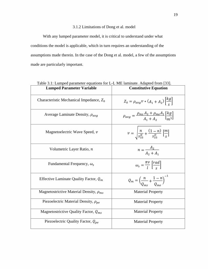
3.1.2 Limitations of Dong et al. model

With any lumped parameter model, it is critical to understand under what

conditions the model is applicable, which in turn requires an understanding of the

assumptions made therein. In the case of the Dong et al. model, a few of the assumptions

made are particularly important.

Table 3.1: Lumped parameter equations for L-L ME laminate. Adapted from [33]. Lumped Parameter Variable Constitutive Equation

Characteristic Mechanical Impedance, 𝑍𝑍0 𝑍𝑍0 = 𝜌𝜌𝑎𝑎𝑎𝑎𝑎𝑎𝑣𝑣 ∗ (𝐴𝐴1 + 𝐴𝐴2) 𝑘𝑘𝑔𝑔𝑠𝑠

Average Laminate Density, 𝜌𝜌𝑎𝑎𝑎𝑎𝑎𝑎 𝜌𝜌𝑎𝑎𝑎𝑎𝑎𝑎 = 𝜌𝜌𝑚𝑚𝑠𝑠 𝐴𝐴2 + 𝜌𝜌𝑚𝑚𝑒𝑒𝐴𝐴1

𝐴𝐴1 + 𝐴𝐴2𝑘𝑘𝑔𝑔𝑚𝑚3

Magnetoelectric Wave Speed, 𝑣𝑣 𝑣𝑣 = 𝑛𝑛𝑠𝑠33𝐻𝐻

+(1 − 𝑛𝑛)𝑠𝑠33𝐷𝐷

𝑚𝑚𝑠𝑠

Volumetric Layer Ratio, 𝑛𝑛 𝑛𝑛 =𝐴𝐴2

𝐴𝐴2 + 𝐴𝐴1

Fundamental Frequency, 𝜔𝜔𝑠𝑠 𝜔𝜔𝑠𝑠 =𝜋𝜋𝑣𝑣𝑙𝑙

𝑟𝑟𝑟𝑟𝑑𝑑𝑠𝑠

Effective Laminate Quality Factor, 𝑄𝑄𝑚𝑚 𝑄𝑄𝑚𝑚 = 𝑛𝑛𝑄𝑄𝑚𝑚𝑠𝑠

+1 − 𝑛𝑛𝑄𝑄𝑚𝑚𝑒𝑒

−1

Magnetostrictive Material Density, 𝜌𝜌𝑚𝑚𝑠𝑠 Material Property

Piezoelectric Material Density, 𝜌𝜌𝑝𝑝𝑒𝑒 Material Property

Magnetostrictive Quality Factor, 𝑄𝑄𝑚𝑚𝑠𝑠 Material Property

Piezoelectric Quality Factor, 𝑄𝑄𝑝𝑝𝑒𝑒 Material Property

20

Mechanically the model makes a very unconservative assumption in that it

assumes that there is perfect and uniform strain transfer from the MS layer into to the PE

layer. This implies that the interface joint between the laminates is taken as infinitely stiff

and that there is no strain gradient through the thickness of the laminate. For the first

implication, this means that if there is some sort of interface between the laminates such

as a compliant epoxy matrix, the model will over predict the ME coefficient and reduce

the effective laminate quality factor. A common mitigation approach to this is to

experimentally measure laminate’s quality factor and use the result to tune the model.

As to the uniform strain assumption, the accuracy varies with the laminate

geometry as well as material properties. Fundamentally, the longer and thinner the

laminate the more accurate this assumption will be, however the relative layer thickness,

as defined by the volumetric layer ratio, 𝑛𝑛, also influence the strain uniformity which

makes it difficult to make a global rule for what point the model geometry is no longer

valid. To date the literature doesn’t report a number for the length to total thickness ratio

of the laminate, however structures with 𝑙𝑙: 𝑡𝑡𝑝𝑝 + 2𝑡𝑡𝑚𝑚 ≥ 5 have been used to

experimentally validate the dong model [29], [34].

Another item to be cautious of is the linear assumption for material properties. For

most properties, such as compliance, it is sufficient to say that for the operating range

experienced, the property is sufficiently linear. But in the case of magnetostriction,

making the appropriate linear assumption takes a bit more work. The piezomagnetic

coefficient is defined as

21

𝑑𝑑33,𝑚𝑚 =𝑑𝑑𝜆𝜆𝑑𝑑𝐻𝐻

(3.9)

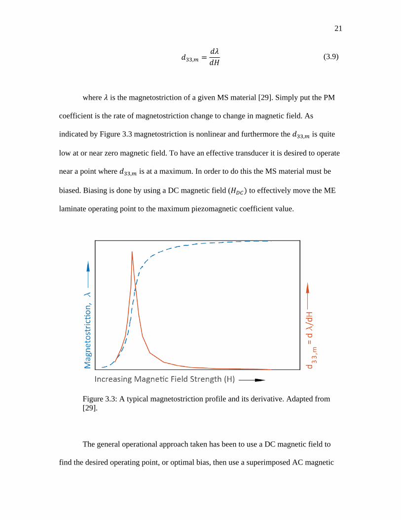
where 𝜆𝜆 is the magnetostriction of a given MS material [29]. Simply put the PM

coefficient is the rate of magnetostriction change to change in magnetic field. As

indicated by Figure 3.3 magnetostriction is nonlinear and furthermore the 𝑑𝑑33,𝑚𝑚 is quite

low at or near zero magnetic field. To have an effective transducer it is desired to operate

near a point where 𝑑𝑑33,𝑚𝑚 is at a maximum. In order to do this the MS material must be

biased. Biasing is done by using a DC magnetic field (𝐻𝐻𝐷𝐷𝐷𝐷) to effectively move the ME

laminate operating point to the maximum piezomagnetic coefficient value.

Figure 3.3: A typical magnetostriction profile and its derivative. Adapted from [29].

The general operational approach taken has been to use a DC magnetic field to

find the desired operating point, or optimal bias, then use a superimposed AC magnetic

22

field of a much smaller amplitude to cause the structure to resonate[29]. To account for

this biasing, which varies tremendously by material, Dong et al. added the variable 𝛽𝛽 to

equation 3.8. A value of 𝛽𝛽 = 1 means the structure is optimally biased; a value of 𝛽𝛽 = 0

means the structure is not biased at all[33]. Much like the quality factor, this component

of the model has to be evaluated experimentally in that the optimal bias varies by

geometry and material selection as well as with any preload induced into the structure.

Work has been done to build self-biased ME structures that eliminate the need for

biasing, however this research is still fairly premature and beyond the scope of this

work[46].

Finally, the last consideration is anchoring. The model presented assumes an

infinitely stiff anchor. Typically, vibrating transducer performance (such as for cantilever

beams) is reduced when anchored to something compliant such as tissue, making this

assumption questionable. However, an advantage to this design, is that due to the

structure’s vibrational symmetry, the equal and opposite motion of extension has a self-

anchoring effect that minimizes loss through the anchor. Given this geometric advantage,

this assumption was deemed suitable for this stage of research.

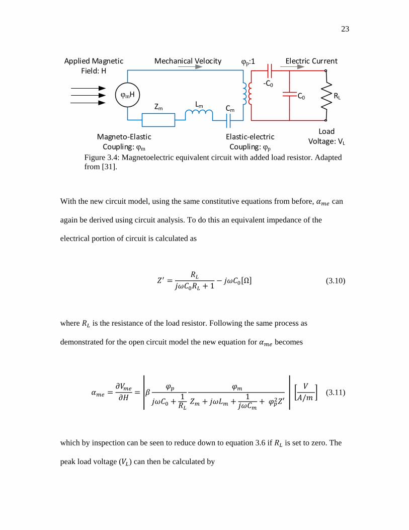
3.1.3 ME Laminate Model for Power Delivery Prediction

To derive the power output of the ME laminate utilizing the Dong et al. model a

load simulating resistor was added to the equivalent circuit as shown in Magnetoelectric

equivalent circuit with added load resistor, adapted from Dong et al. [30].

23

Lm Zm Cm

φmH

φp:1

C0

-C0

Load Voltage: VL

Applied MagneticField: H

Mechanical Velocity Electric Current

Magneto-ElasticCoupling: φm

Elastic-electric Coupling: φp

RL

Figure 3.4: Magnetoelectric equivalent circuit with added load resistor. Adapted from [31].

With the new circuit model, using the same constitutive equations from before, 𝛼𝛼𝑚𝑚𝑒𝑒 can

again be derived using circuit analysis. To do this an equivalent impedance of the

electrical portion of circuit is calculated as

𝑍𝑍′ =𝑅𝑅𝐿𝐿

𝑗𝑗𝜔𝜔𝐶𝐶0𝑅𝑅𝐿𝐿 + 1− 𝑗𝑗𝜔𝜔𝐶𝐶0[Ω] (3.10)

where 𝑅𝑅𝐿𝐿 is the resistance of the load resistor. Following the same process as

demonstrated for the open circuit model the new equation for 𝛼𝛼𝑚𝑚𝑒𝑒 becomes

𝛼𝛼𝑚𝑚𝑒𝑒 =𝜕𝜕𝑉𝑉𝑚𝑚𝑒𝑒

𝜕𝜕𝐻𝐻= 𝛽𝛽

𝜑𝜑𝑝𝑝

𝑗𝑗𝜔𝜔𝐶𝐶0 + 1𝑅𝑅𝐿𝐿

𝜑𝜑𝑚𝑚

𝑍𝑍𝑚𝑚 + 𝑗𝑗𝜔𝜔𝐿𝐿𝑚𝑚 + 1𝑗𝑗𝜔𝜔𝐶𝐶𝑚𝑚

+ 𝜑𝜑𝑝𝑝2𝑍𝑍′

𝑉𝑉𝐴𝐴/𝑚𝑚

(3.11)

which by inspection can be seen to reduce down to equation 3.6 if 𝑅𝑅𝐿𝐿 is set to zero. The

peak load voltage (𝑉𝑉𝐿𝐿) can then be calculated by

24

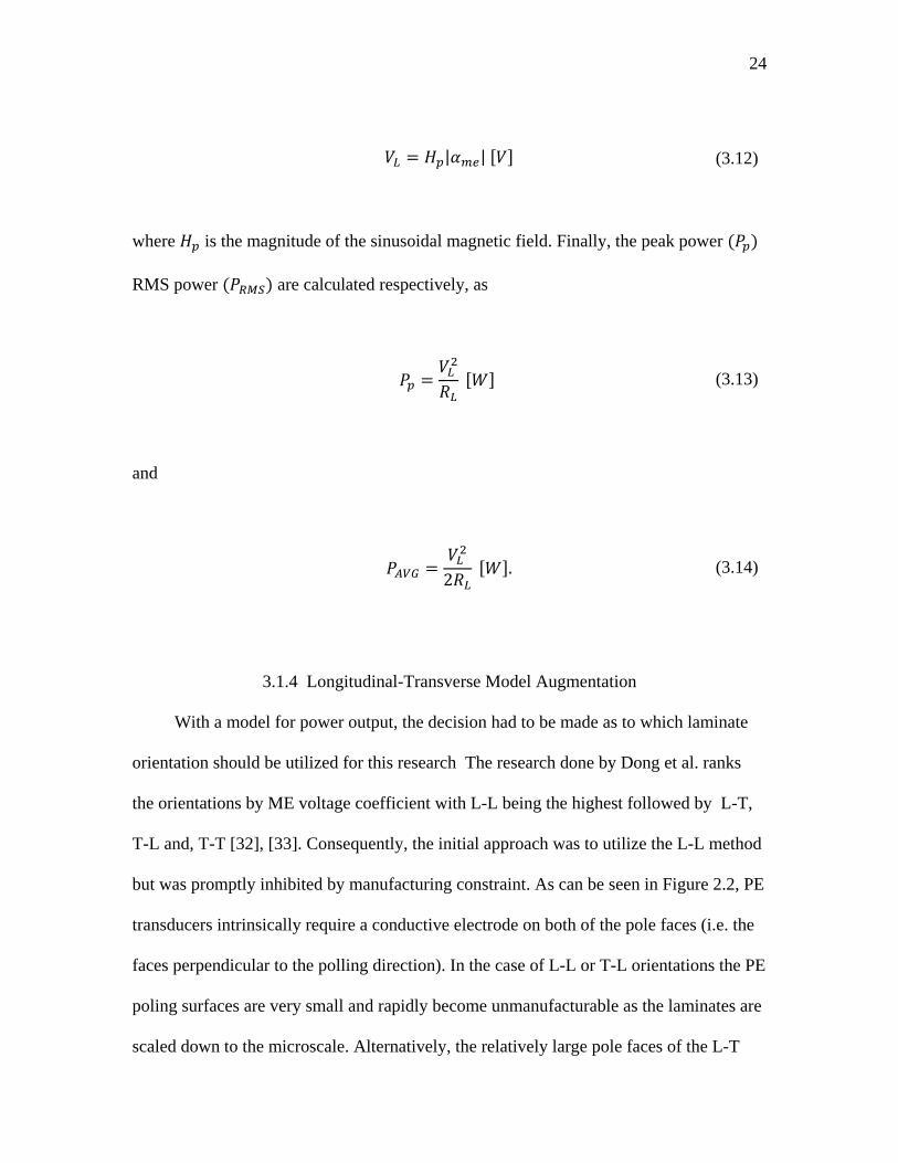
𝑉𝑉𝐿𝐿 = 𝐻𝐻𝑝𝑝|𝛼𝛼𝑚𝑚𝑒𝑒| [𝑉𝑉] (3.12)

where 𝐻𝐻𝑝𝑝 is the magnitude of the sinusoidal magnetic field. Finally, the peak power (𝑃𝑃𝑝𝑝)

RMS power (𝑃𝑃𝑂𝑂𝑀𝑀𝑂𝑂) are calculated respectively, as

𝑃𝑃𝑝𝑝 =𝑉𝑉𝐿𝐿2

𝑅𝑅𝐿𝐿 [𝑊𝑊] (3.13)

and

𝑃𝑃𝐴𝐴𝐴𝐴𝐴𝐴 =𝑉𝑉𝐿𝐿2

2𝑅𝑅𝐿𝐿 [𝑊𝑊]. (3.14)

3.1.4 Longitudinal-Transverse Model Augmentation

With a model for power output, the decision had to be made as to which laminate

orientation should be utilized for this research The research done by Dong et al. ranks

the orientations by ME voltage coefficient with L-L being the highest followed by L-T,

T-L and, T-T [32], [33]. Consequently, the initial approach was to utilize the L-L method

but was promptly inhibited by manufacturing constraint. As can be seen in Figure 2.2, PE

transducers intrinsically require a conductive electrode on both of the pole faces (i.e. the

faces perpendicular to the polling direction). In the case of L-L or T-L orientations the PE

poling surfaces are very small and rapidly become unmanufacturable as the laminates are

scaled down to the microscale. Alternatively, the relatively large pole faces of the L-T

25

and T-T laminates mitigate this problem and can allow for the circuit to even be passed

through the conductive MS layer, simplifying attaching leads to the laminate. Based on

the literature ranking, the obvious next best configuration for this study was L-T.

Based on this change, corrections in the previous model had to be made to reflect

the new geometry layout as seen in Figure 3.5. The general equivalent circuit remained

unchanged however, due to the change in orientation, equations involving the properties

of the PM had to be updated. Particularly the piezoelectric voltage coefficient and elastic

compliance became 𝑔𝑔31,𝑝𝑝 and 𝑠𝑠11𝐷𝐷 respectively now that the strain field was perpendicular

to the poling direction. Also, the piezoelectric coupling factor was rederived as

𝜑𝜑𝑝𝑝 = 𝐴𝐴1𝑔𝑔31,𝑝𝑝

𝑡𝑡𝑝𝑝𝑠𝑠33𝐷𝐷 𝛽𝛽𝑝𝑝 𝑁𝑁𝑉𝑉. (3.15)

A summary of the affected equations is shown in Table 3.2. By implementing these

equations with others presented previously, the theoretical performance of the L-T

configured laminate can be calculated.

26

lM

M

P P A1

A2/2

A2/2

A

A A-A

PEMS

MStp

wtm

Figure 3.5: Geometry layout for L-T mode bimorph, arrows M and P show the magnetization and polarization orientation, adapted from [31].

Table 3.2: Corrected lumped parameters for L-T configuration [33]. Lumped Parameter Variable Constitutive Equation

Effective Inverse PE Dielectric Constant, 𝛽𝛽𝑝𝑝 𝛽𝛽𝑝𝑝 = 𝛽𝛽𝑝𝑝 1 +𝑔𝑔332

𝑠𝑠33𝐷𝐷 𝛽𝛽𝑝𝑝 𝑀𝑀𝐹𝐹

Piezoelectric Capacitance, 𝐶𝐶0 𝐶𝐶0 = 𝑤𝑤𝑙𝑙𝑡𝑡𝑝𝑝 𝛽𝛽𝑝𝑝

[𝐹𝐹]

Magnetoelectric Wave Speed, 𝑣𝑣 𝑣𝑣 = 𝑛𝑛𝑠𝑠33𝐻𝐻

+(1 − 𝑛𝑛)𝑠𝑠11𝐷𝐷

𝑚𝑚𝑠𝑠

27

3.2 Lumped Parameter Model for MME “Butterfly” Transducer

The second lumped element model to be discussed is that of the Mechano-

Magnetoelectric (MME) transducer. Unlike the ME laminate model, there is not a well

published lumped model for the specific geometry under consideration. Subsequently, the

following lumped element model was obtained from a yet to be published parallel effort

performed by Binh Duc Truong and Dr. Shad Roundy of the University of Utah’s

Integrated Self-powered Sensing Lab. The entire derivation can be found in [47].

3.2.1 MME Geometry and Model Summary

The new geometry proposed as shown in Figure 3.6, utilizes a single pizeoelectric

bending laminate composed of a PE top sheet, a structural center sheet (Ssub), and another

symetric PE bottom sheet to couple bending strain to an electric field. Strain is induced

on the structure by anchoring the bending laminate in the center and adding opposite

oriented permanent magnets at its ends. When a magnetic field is applied along the length

of the structure the effect is a symetric cantilever or bending motion.

By making the structure a double cantilever beam, much like the ME bimorph, the

stress transmitted through the anchor is ideally reduced to zero due to the counteracting

motions of the two beams. This in turn means that anchor losses in mediums such as

tissue should also be reduced.

The equivalent circuit model for the structure is shown in Figure 3.7. By

inspection it can be seen that the model is fundamentally similar to the ME laminate

model and shares the same parameters for the piezoelectric portion of the circuit.

28

PA

A

A-A

Ssub tsw

tp

P

HDCHDC

2L

L0 LmL

PEPE

PMh

Figure 3.6: Geometry layout for the double cantilever MME structure. Arrows marked P indicate PE poling directions and arrows marked Hdc Indicate the orientation of the permanent magnetic fields.

Fm

φp:1

C0

Load Voltage: VL

Applied MagneticField: H

Beam Tip Deflection Electric Current

Equivalent Force from Magnet: Fm

Elastic-electric Coupling: φp

RL

m 1/K0b

Figure 3.7: Lumped element equivalent circuit of double cantilever MME structure

29

The power output of the MME is calculated as

𝑃𝑃 =12∆𝐾𝐾

𝜔𝜔2𝜏𝜏1 + 𝜔𝜔2𝜏𝜏

|𝑋𝑋0|2 [𝑊𝑊]. (3.16)

where

𝜏𝜏 = 𝑅𝑅𝐿𝐿𝐶𝐶0 [𝑠𝑠], (3.17)

∆𝐾𝐾 =𝜑𝜑𝑝𝑝2

𝐶𝐶0 𝑁𝑁𝑚𝑚, (3.18)

𝜑𝜑𝑝𝑝 = −

4𝑒𝑒31𝑤𝑤2𝑡𝑡𝑝𝑝 + 𝑡𝑡𝑠𝑠[3(𝑀𝑀 + 𝑚𝑚𝑏𝑏)𝐿𝐿2 − 3𝑚𝑚𝑏𝑏𝐿𝐿0𝐿𝐿 + 𝑚𝑚𝑏𝑏𝐿𝐿02]6(𝑀𝑀 + 𝑚𝑚𝑏𝑏)𝐿𝐿3 − 6𝑚𝑚𝑏𝑏𝐿𝐿0𝐿𝐿2 + 2𝐿𝐿02𝐿𝐿(𝑀𝑀 + 2𝑚𝑚𝑏𝑏) − 𝐿𝐿03𝑚𝑚𝑏𝑏

𝑁𝑁𝑉𝑉,

(3.19)

and

|𝑋𝑋0|2 =𝐹𝐹𝑜𝑜2

𝜔𝜔𝑏𝑏 + ∆𝐾𝐾 𝜔𝜔𝜏𝜏1 + (𝜔𝜔𝜏𝜏)2

2+ 𝐾𝐾1 − 𝑚𝑚𝜔𝜔2 − ∆K 1

1 + (𝜔𝜔𝜏𝜏)22

[𝑚𝑚2] (3.20)

At optimal load resistance and natural frequency, the optimal average power is

stated as

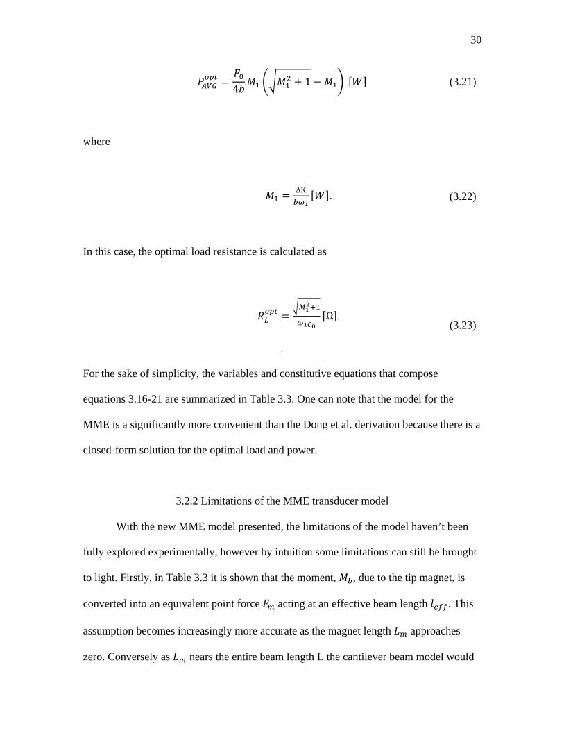
30

𝑃𝑃𝐴𝐴𝐴𝐴𝐴𝐴𝑜𝑜𝑝𝑝𝑜𝑜 =

𝐹𝐹04𝑏𝑏

𝑀𝑀1 𝑀𝑀12 + 1 −𝑀𝑀1 [𝑊𝑊] (3.21)

where

𝑀𝑀1 = ∆K𝑏𝑏𝜔𝜔1

[𝑊𝑊]. (3.22)

In this case, the optimal load resistance is calculated as

𝑅𝑅𝐿𝐿𝑜𝑜𝑝𝑝𝑜𝑜 =

𝑀𝑀12+1

𝜔𝜔1𝐶𝐶0[Ω].

.

(3.23)

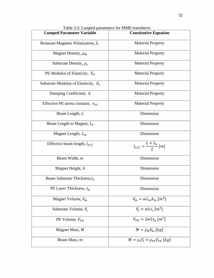
For the sake of simplicity, the variables and constitutive equations that compose

equations 3.16-21 are summarized in Table 3.3. One can note that the model for the

MME is a significantly more convenient than the Dong et al. derivation because there is a

closed-form solution for the optimal load and power.

3.2.2 Limitations of the MME transducer model

With the new MME model presented, the limitations of the model haven’t been

fully explored experimentally, however by intuition some limitations can still be brought

to light. Firstly, in Table 3.3 it is shown that the moment, 𝑀𝑀𝑏𝑏, due to the tip magnet, is

converted into an equivalent point force 𝐹𝐹𝑚𝑚 acting at an effective beam length 𝑙𝑙𝑒𝑒𝑒𝑒𝑒𝑒. This

assumption becomes increasingly more accurate as the magnet length 𝐿𝐿𝑚𝑚 approaches

zero. Conversely as 𝐿𝐿𝑚𝑚 nears the entire beam length L the cantilever beam model would

31

be better described by a distributed load. The experiments done by Truong and Roundy,

which were well correlated to their model, used a structure with an 𝐿𝐿𝑚𝑚: 𝐿𝐿 ratio of 1:4.8. It

remains to be shown what the upper limit for the ratio of 𝐿𝐿𝑚𝑚: 𝐿𝐿 should be, but for the sake

of this research it will be taken slightly conservatively as less than 1:4.

Another factor that the model overlooks is the strength of the beam itself,

particularly the piezoelectric material. In fact, it is possible that the beam strength for the

MME drives the 𝐿𝐿𝑚𝑚: 𝐿𝐿 ratio as much as the model’s equivalent force assumption. In a

linear model such as that presented by Truong and Roundy, an optimization of this model

would likely lead to large magnets and large deflections, which may or may not be

mechanically feasible. However, most piezoelectric materials are brittle and can fracture

quiet easily so it is important to bound the structure design by ensuring that the bending

strength of the PE material is not exceeded by the tip magnet. How this bounding can be

done will be discussed in Chapter 5.

32

Table 3.3: Lumped parameters for MME transducer. Lumped Parameter Variable Constitutive Equation

Remnant Magnetic Polarization, 𝐽𝐽𝑟𝑟 Material Property

Magnet Density, 𝜌𝜌𝑀𝑀 Material Property

Substrate Density, 𝜌𝜌𝑠𝑠 Material Property

PE Modulus of Elasticity, 𝐸𝐸𝑃𝑃 Material Property

Substrate Modulus of Elasticity, 𝐸𝐸𝑠𝑠 Material Property

Damping Coefficient, 𝑏𝑏 Material Property

Effective PE stress constant, 𝑒𝑒33 Material Property

Beam Length, 𝐿𝐿 Dimension

Beam Length to Magnet, 𝐿𝐿0 Dimension

Magnet Length, 𝐿𝐿𝑚𝑚 Dimension

Effective beam length, 𝑙𝑙𝑒𝑒𝑒𝑒𝑒𝑒 𝑙𝑙𝑒𝑒𝑒𝑒𝑒𝑒 =𝐿𝐿 + 𝐿𝐿0

2[𝑚𝑚]

Beam Width, 𝑤𝑤 Dimension

Magnet Height, ℎ Dimension

Beam Substrate Thickness,𝑡𝑡𝑠𝑠 Dimension

PE Layer Thickness, 𝑡𝑡𝑝𝑝 Dimension

Magnet Volume, 𝑉𝑉𝑚𝑚 𝑉𝑉𝑚𝑚 = 𝑤𝑤𝐿𝐿𝑚𝑚ℎ𝑚𝑚 [𝑚𝑚3]

Substrate Volume, 𝑉𝑉𝑠𝑠 𝑉𝑉𝑠𝑠 = 𝑤𝑤𝐿𝐿𝑡𝑡𝑠𝑠 [𝑚𝑚3]

PE Volume, 𝑉𝑉𝑃𝑃𝑃𝑃 𝑉𝑉𝑃𝑃𝑃𝑃 = 2𝑤𝑤𝐿𝐿𝑡𝑡𝑝𝑝 [𝑚𝑚3]

Magnet Mass, 𝑀𝑀 𝑀𝑀 = 𝜌𝜌𝑀𝑀𝑉𝑉𝑚𝑚 [𝑘𝑘𝑔𝑔]

Beam Mass, 𝑚𝑚 𝑀𝑀 = 𝜌𝜌𝑠𝑠𝑉𝑉𝑠𝑠 + 𝜌𝜌𝑃𝑃𝑃𝑃𝑉𝑉𝑃𝑃𝑃𝑃 [𝑘𝑘𝑔𝑔]

33

Table 3.3: Continued Beam Mass, 𝑚𝑚𝑏𝑏 𝑚𝑚𝑏𝑏 = 𝜌𝜌𝑠𝑠𝑉𝑉𝑠𝑠 + 𝜌𝜌𝑃𝑃𝑃𝑃𝑉𝑉𝑃𝑃𝑃𝑃 [𝑘𝑘𝑔𝑔]

Equivalent Mass, 𝑚𝑚 𝑚𝑚 = 𝑀𝑀 + 33140

𝑚𝑚𝑏𝑏 [m]

Magnet Moment, 𝑀𝑀𝑏𝑏 𝑀𝑀𝑏𝑏 = 𝐽𝐽𝑟𝑟𝑉𝑉𝑚𝑚𝐻𝐻𝐴𝐴𝐷𝐷 [Nm]

Equivalent Moment Force, 𝐹𝐹𝑚𝑚 𝐹𝐹𝑀𝑀 =3𝑀𝑀𝑏𝑏

2𝑙𝑙𝑒𝑒𝑒𝑒𝑒𝑒[𝑁𝑁]

Short-circuit Stiffness, 𝐾𝐾0 𝐾𝐾0 =

3(𝑌𝑌𝐸𝐸)𝑐𝑐𝑙𝑙𝑒𝑒𝑒𝑒𝑒𝑒3

𝑁𝑁𝑚𝑚

Optimal Load Stiffness 𝐾𝐾1 = 𝐾𝐾0 + ∆𝐾𝐾 𝑁𝑁𝑚𝑚

Composite Flexural Rigidity, (𝐸𝐸𝐸𝐸)𝑐𝑐 (𝐸𝐸𝐸𝐸)𝑐𝑐 = 2𝐸𝐸𝑝𝑝 2𝑤𝑤𝑡𝑡𝑝𝑝3

12+ 2𝑤𝑤𝑡𝑡𝑝𝑝

𝑡𝑡𝑠𝑠 + 2𝑜𝑜𝑝𝑝2

2

+ 𝐸𝐸𝑠𝑠𝑤𝑤𝑡𝑡𝑠𝑠3

12 [𝑁𝑁𝑚𝑚2]

Piezoelectric Capacitance, 𝐶𝐶0 𝐶𝐶0 = 𝑤𝑤𝑙𝑙

2𝑡𝑡𝑝𝑝𝛽𝛽𝑝𝑝 [𝐹𝐹]

Loaded Natural Frequency, 𝜔𝜔1 𝜔𝜔1 = 𝐾𝐾1

𝑚𝑚 𝑟𝑟𝑟𝑟𝑑𝑑𝑠𝑠

CHAPTER 4

EXPERIMENTAL VALIDATION OF TRANSDUCER MODELS

To ensure that the models being implemented into the numerical optimization

study yielded credible results, particularly with regard to the power output, it was

necessary to verify them experimentally. The chosen approach was to build millimeter

(as opposed to micrometer) scale transducers, characterize them, and then compare their

characterization data with the model predictions. Millimeter scale transducers were used

to avoid prematurely expending time and resources on a microfabricated design before

completion of the optimization.

4.1 Experimental Setup

In order to characterize any ME transducer a well understood magnetic field must

be generated to serve as a baseline transmitter. In this case it was decided to build a single

axis nested Helmholtz Coil, given their exceptional magnetic field uniformity.

Leveraging work done by Abbott on nesting tri-axial coils, the field generator was

designed with an exterior DC coil pair and a nested AC coil pair built in such a way to

allow for uniform superimposition of fields[48]. By superimposing the two fields, ME

transducers could be both biased with the DC field and driven with the AC field. The

diagram for this setup is shown in Figure 4.1

35

Figure 4.1: Magnetoelectric transducer experimental test setup diagram.

4.1.1 Nested Helmholtz Coil Design

The performance goal of the setup was to deliver an AC magnetic field (𝐻𝐻𝑝𝑝) of 2-

Oe (2 G in air) at 150 kHz with a 40-Watt 50Ω amplifier with no additional circuitry (IE

tuned resonating capacitors) and a DC magnetic field (𝐻𝐻𝐷𝐷𝐷𝐷) of 16-Oe without exceeding

the safe wire gauge current. Subsequently, the geometry of the coils was bounded by the

minimum active area needed to fit transducers and the maximum coil size that could be

driven with accessible amplifiers. Using the equations from Abbott’s paper to

approximate magnetic field levels, the geometry in Table 4.1 was produced[48].

Table 4.1: Nested Helmholtz Coil geometry. Specification AC Coil DC Coil

Coil diameter (center of cross-section) 91 133 mm

Nominal coil cross-section 4.9 mm x 4.9 mm 4.9 mm x 4.9 mm

Optimal coil separation spacing 46 mm 67 mm

Wire gauge 16 20

Number of turns 9 25

Signal Generator

Amplifier

Current Clamp

DC Power Supply

Transducer

Oscilloscope

Transducer Voltage RLNested

Helmholtz Coil

36

4.1.2Nested Helmholtz Coil Performance

The geometry resulted in the built device shown in Figure 2.1. Built with 3D printed ABS

and hand coiled copper magnet wire, the produced field was found to be very uniform.

Using an AlphaLab UHS2 gauss meter, the AC coil was measured to have only 2% field

variation over ±1.5 cm at the coil origin (the point colinear to the coil axis and equidistant

from the inner coil faces) along the axial center line. The DC coil had less than 5%

variation over the same length. For this and all other work the AC coil was driven by a

Tektronix AFG1022 signal generator and either a E&I 210 or a Rigol PA1011 amplifier.

The DC coils were driven with a B&K Precision 9201 power supply.

DEVICE UNDER TEST

AC COIL

DC COIL

Figure 4.2: Nested Helmholtz Coil built for experimental validation.

37

Given the difficulty of measuring AC magnetic fields during experiments with

ME and MME transducers, the linear relationship of electric current to field strength was

used to create a calibration curve. This was done for the AC coils by measuring field

magnitude at the coil origin while a 10kHz driving current was increased, ensuring that

the DC coils were shorted out. To characterize the DC coils, the process was reversed,

driving them under an AC load to utilize the same AC sensor, ensuring that the AC coils

were now shorted. By so doing the coil field strength could be monitored from the output

of a current clamp rather than a bulky, narrow frequency AC magnetic field sensor during

any subsequent ME transducer testing. Also, to get a better understanding of the coils,

their inductance was measured using a circuit analyzer. The results of this coil

characterization are shown in Table 4.2.

Table 4.2: Built nested Helmholtz Coil performance and predictions. AC Coil DC Coil

Optimal Spacing 52 mm Driven by AC Coil

Total inductance predicated 7.3 µH 88 µH

Total inductance measured (alternate coil open circuit)

38 µH 410µH

Total inductance measured (alternate coil short circuit)

30 µH Not Measured

Coil calibration (alternate coil short circuit)

.502 Oe/A (R2=.9998) 1.350 Oe/A (R2=.9999)

Predicted field levels 2 Oe Peak at 150Khz & 40W 16 Oe at 6A DC

Realized field levels .5 Oe Peak at 150kHz & 40W 8.1 Oe at 6A DC

38

From examination of the table it is seen that both the field performance and

predicted inductance were far below the design predictions made. In reviewing the

equations used, the discrepancy was explained as it became evident that the

approximations from Abbott were better suited for coils with much smaller diameter wire

and a great number of turns[48]. Additionally, the work done here also failed to account

for the reduction in performance caused by the coupled inducive effect of nesting two

sets of coils on the same axis. All told, enough margin was given for the desired field

levels that the design was still useful for this research. Nonetheless, a better method for

design of coils for ME transducers should be implemented, or at the very least, a design

should be verified before manufacture with another tool such as FEA.

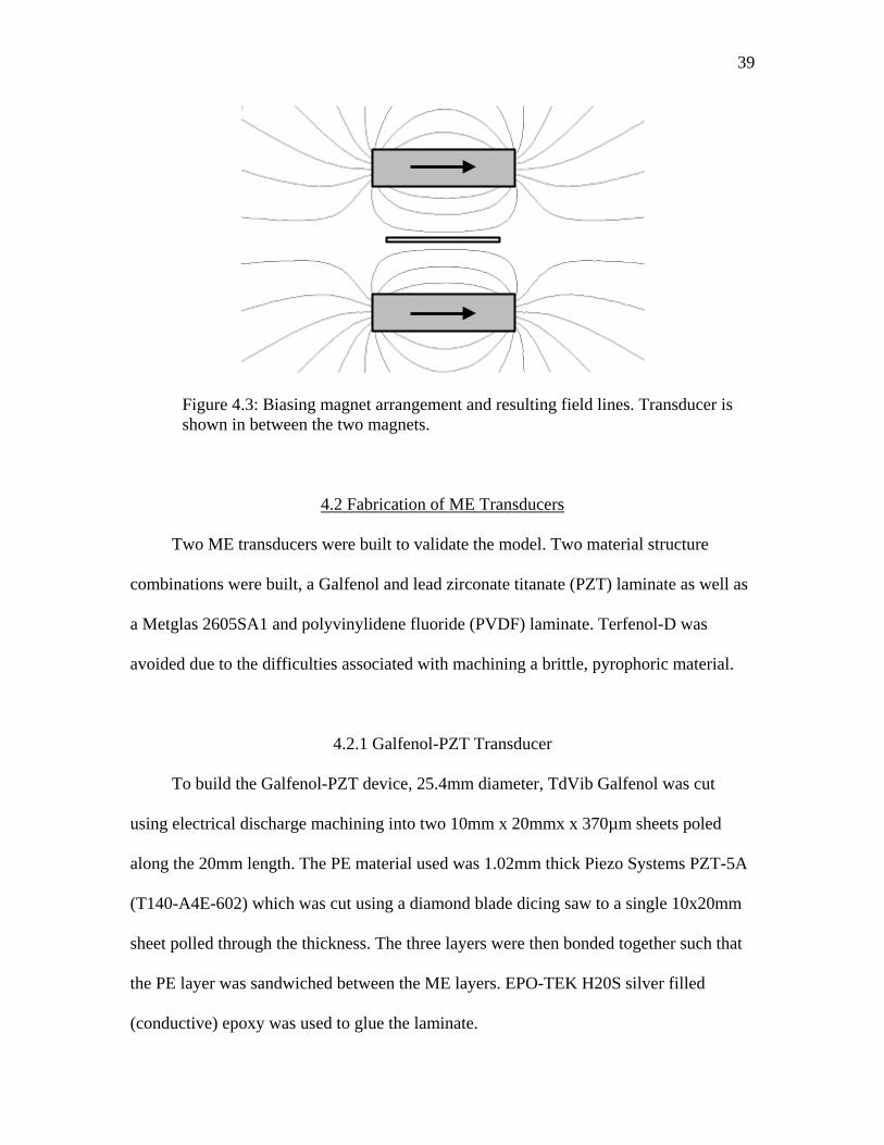
4.1.3 Additional DC Field Biasing Measures

During this work it became evident that it would be difficult to build DC coils

large enough to bias structures made of Galfenol or Terfenol-D. As built the DC coils

were capable of biasing Metglas structures which requires a bias on the order of 1-10 Oe

[29]. To bias Galfenol or Terfenol-D, which require bias fields 100s of Oe, many

different approaches can be taken[30]. Two parallel N52 Neodymium magnets were used

as shown in Figure 4.3. By adjusting the distance between the two magnets with a 3d

printed stage as shown in Figure 4.5 the field seen by the centered transducer can be

adjusted such that 𝛽𝛽 = 1.

39

Figure 4.3: Biasing magnet arrangement and resulting field lines. Transducer is shown in between the two magnets.

4.2 Fabrication of ME Transducers

Two ME transducers were built to validate the model. Two material structure

combinations were built, a Galfenol and lead zirconate titanate (PZT) laminate as well as

a Metglas 2605SA1 and polyvinylidene fluoride (PVDF) laminate. Terfenol-D was

avoided due to the difficulties associated with machining a brittle, pyrophoric material.

4.2.1 Galfenol-PZT Transducer

To build the Galfenol-PZT device, 25.4mm diameter, TdVib Galfenol was cut

using electrical discharge machining into two 10mm x 20mmx x 370µm sheets poled

along the 20mm length. The PE material used was 1.02mm thick Piezo Systems PZT-5A

(T140-A4E-602) which was cut using a diamond blade dicing saw to a single 10x20mm

sheet polled through the thickness. The three layers were then bonded together such that

the PE layer was sandwiched between the ME layers. EPO-TEK H20S silver filled

(conductive) epoxy was used to glue the laminate.

40

The epoxy was cured using a heat press, following the epoxy’s minimum cure

instructions. Finally, two .635 mm right angle header pins were bonded to the top and

bottom Galfenol. This bond was done using MG Chemicals silver conductive epoxy

given that the joint wasn’t structural. This epoxy was cured overnight at room

temperature. The resulting transducer can be seen in Figure 4.4

Figure 4.4: Galfenol-PZT ME transducer, shown anchored at its center (left), and zoomed in on the cross section (right).

4.2.2 Metglas-PVDF transducer

The Metglas-PVDF device was built in a fashion similar to that of the Galfenol-

PZT. Raw 23µm thick 2605SA1 Metglas was cut using scissors into two 10x20mm

layers. The nature of amorphous Metglas is such that magnetostriction occurs at any

orientation in the sheet plane so poling direction was unimportant. To match the very thin

Metglas, metalized PVDF (TE 1-1004347-0) was used. These sheets themselves were a

41

sandwich of 28µm PVDF with 6µm silver ink electrodes on the top and the bottom, poled

through the thickness.

These sheets were also cut to 10x20mm; however, a small tab was left so that

electrical leads could be attached to the PE while using a non-conductive epoxy. In

particular the nonconductive epoxy EPO-TEK H70E was used for its slightly thinner

minimum bond line of less than 20 µm compared to the silver filled alternative which

was measured on the Galfenol-PZT device to be about 35 µm. As before, the epoxy was

cured in a heat press at the minimum prescribed cure. Similar leads were also bonded as

before, however this time on the center flange of the PVDF. The final structure can be

seen in Figure 4.5.

Figure 4.5: Metglas-PVDF ME transducer with bonded leads visible.

42

4.3 Galfenol-PZT Device Characterization and Model Comparison

The structures were characterized, beginning with the Galfenol-PZT device. The

process to do so began with first optimizing the magnetic bias field. Next open circuit

frequency sweeps were done to determine the structure’s natural frequency and the

system’s repeatability. Finally, loaded circuit frequency sweeps and load optimization

were done.

4.3.1 Optimal Bias Field

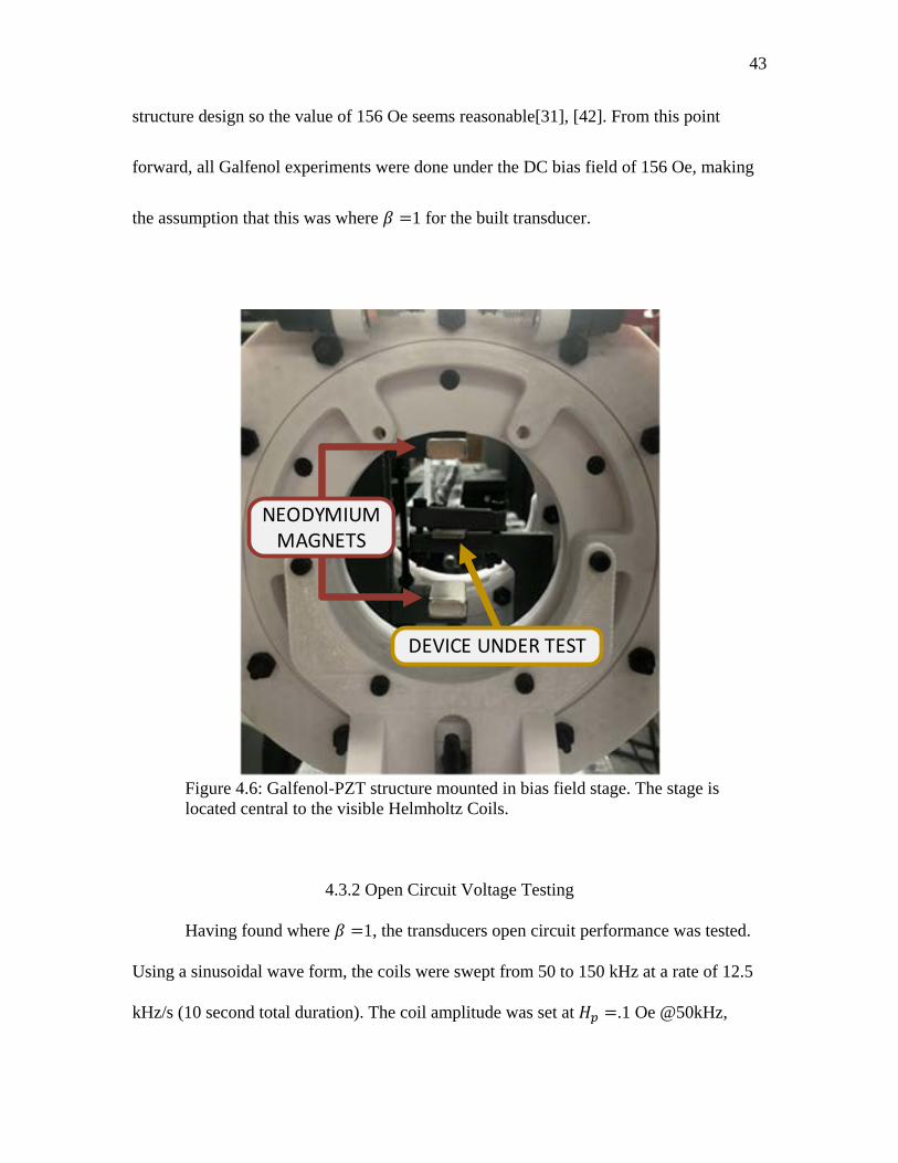
To determine the optimal field bias for the transducer it was mounted between

two adjustable magnets as shown in Figure 4.6. While operating the coils at 70 kHz (near

resonance), the open circuit output voltage of the transducer was measured as the distance

between the transducer and the magnets was varied. The distance between the magnet’s

inner faces, for which voltage was maximized, was found to be 1.70 inches. The

transducer was located in the center as is shown. Moving the magnets closer or further

apart diminished voltages as the structure became over or under biased respectively.

The DC bias field component parallel to the transducer length was measured

along the length of the transducer with an Alphalab GM1-ST DC gauss meter yielding an

average strength of 156 Oe with ±20 Oe deviation from average across the length of the

device. Literature for bias field levels of Galfenol transducers is sparse, however for

stiffer Terfenol-D transducers have reported bias fields of 200-500 Oe, depending on the

43

structure design so the value of 156 Oe seems reasonable[31], [42]. From this point

forward, all Galfenol experiments were done under the DC bias field of 156 Oe, making

the assumption that this was where 𝛽𝛽 =1 for the built transducer.

DEVICE UNDER TEST

NEODYMIUM MAGNETS

Figure 4.6: Galfenol-PZT structure mounted in bias field stage. The stage is located central to the visible Helmholtz Coils.

4.3.2 Open Circuit Voltage Testing

Having found where 𝛽𝛽 =1, the transducers open circuit performance was tested.

Using a sinusoidal wave form, the coils were swept from 50 to 150 kHz at a rate of 12.5

kHz/s (10 second total duration). The coil amplitude was set at 𝐻𝐻𝑝𝑝 =.1 Oe @50kHz,

44

however this value attenuated as the sweep progressed due to the increasing coil

impedance. To compensate for this the magnetic field level and open circuit transducer

voltage were measured simultaneously and then normalized for all of the sweeps done.

The normalization was done by performing an FFT on the signals then dividing

the resulting transducer voltage amplitude by the field amplitude. The result, known as a

linear transfer function, was then multiplied by 𝐻𝐻𝑂𝑂𝑀𝑀𝑂𝑂 =.707 Oe to find the open circuit

RMS voltage, 𝑉𝑉𝑂𝑂𝑂𝑂𝑀𝑀𝑂𝑂, across the sweep frequency. It should be noted that this

normalization does make the assumption that the transducer performance is linear, as

does the model to which it will be compared. This assumption is common for many

transducers and was validated experimentally for the ME transducer design by Bian et al

[49].

For these first open circuit tests, to ensure that the results were repeatable, the

transducer was swept nine times. Additionally, after each sweep the stage holding the

transducer was removed then replaced; after every 3rd sweep the transducer was also

removed from the bias structure entirely then re-clamped. The results of these sweeps can

be seen in Figure 4.6

By examining the plots, it is evident that the system is quite consistent in that at

natural frequency the standard deviation is only about 4.5% of the average value. The

average natural frequency (𝜔𝜔𝑠𝑠) of the system was found to be 71.3 kHz with an average

quality factor 𝑄𝑄𝑚𝑚 of 62.65.

45

Figure 4.7: Repeated open circuit voltage vs frequency. Experimental Average, upper and lower deviation and model prediction shown.

4.3.3 Tuned Comparison Model

Also shown in Figure 4.6 is a curve for what the Dong et al. model predicted for

the structure performance. The model was fed the geometric parameters of the tested

structure and the material properties shown in Table 4.3. By matching the model’s quality

factor to that of the experiment and choosing 𝑑𝑑33,𝑚𝑚 =15 𝑛𝑛𝑚𝑚/𝐴𝐴, it is evident that the open

circuit model matches the experimental result quite well.

46

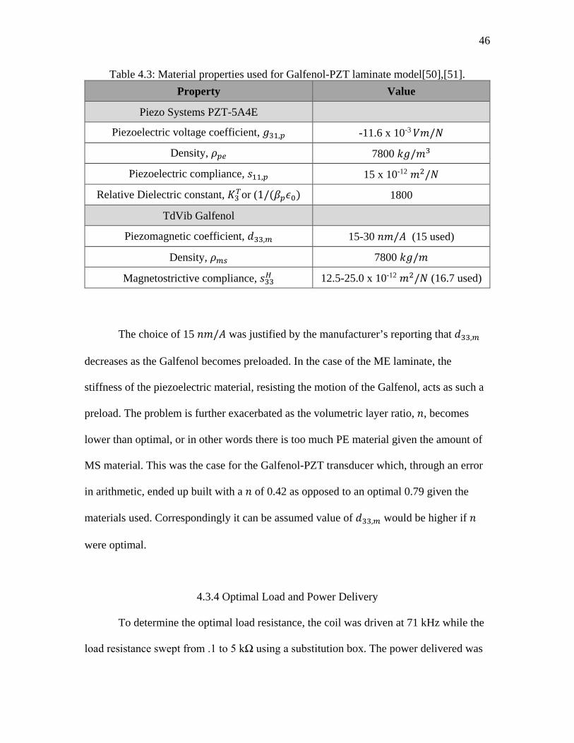
Table 4.3: Material properties used for Galfenol-PZT laminate model[50],[51]. Property Value

Piezo Systems PZT-5A4E

Piezoelectric voltage coefficient, 𝑔𝑔31,𝑝𝑝 -11.6 x 10-3 𝑉𝑉𝑚𝑚/𝑁𝑁

Density, 𝜌𝜌𝑝𝑝𝑒𝑒 7800 𝑘𝑘𝑔𝑔/𝑚𝑚3

Piezoelectric compliance, 𝑠𝑠11,𝑝𝑝 15 x 10-12 𝑚𝑚2/𝑁𝑁

Relative Dielectric constant, 𝐾𝐾3𝑇𝑇or (1/(𝛽𝛽𝑝𝑝𝜖𝜖0) 1800

TdVib Galfenol

Piezomagnetic coefficient, 𝑑𝑑33,𝑚𝑚 15-30 𝑛𝑛𝑚𝑚/𝐴𝐴 (15 used)

Density, 𝜌𝜌𝑚𝑚𝑠𝑠 7800 𝑘𝑘𝑔𝑔/𝑚𝑚

Magnetostrictive compliance, 𝑠𝑠33𝐻𝐻 12.5-25.0 x 10-12 𝑚𝑚2/𝑁𝑁 (16.7 used)

The choice of 15 𝑛𝑛𝑚𝑚/𝐴𝐴 was justified by the manufacturer’s reporting that 𝑑𝑑33,𝑚𝑚

decreases as the Galfenol becomes preloaded. In the case of the ME laminate, the

stiffness of the piezoelectric material, resisting the motion of the Galfenol, acts as such a

preload. The problem is further exacerbated as the volumetric layer ratio, 𝑛𝑛, becomes

lower than optimal, or in other words there is too much PE material given the amount of

MS material. This was the case for the Galfenol-PZT transducer which, through an error

in arithmetic, ended up built with a 𝑛𝑛 of 0.42 as opposed to an optimal 0.79 given the

materials used. Correspondingly it can be assumed value of 𝑑𝑑33,𝑚𝑚 would be higher if 𝑛𝑛

were optimal.

4.3.4 Optimal Load and Power Delivery

To determine the optimal load resistance, the coil was driven at 71 kHz while the

load resistance swept from .1 to 5 kΩ using a substitution box. The power delivered was

47

then calculated using the measured voltage across the load resistance. The results of this

procedure are seen in Figure 4.8.

Figure 4.8: Power output vs load resistance for Galfenol-PZT device operating at 71 kHz.

In particular, the transducer was found to have a max 𝑃𝑃𝐴𝐴𝐴𝐴𝐴𝐴 of 5.01 mW at 𝑅𝑅𝐿𝐿 =

2.3kΩ as compared to the model which predicted the max 𝑃𝑃𝐴𝐴𝐴𝐴𝐴𝐴 to be 9.95 mW at 𝑅𝑅𝐿𝐿 =

1.9kΩ. These results were promising in that the load resistance and curve shape of the

experiment were sufficiently similar to that of the model. For the Galfenol-PZT

transducer the model also overpredicted power delivery by almost double what was found

experimentally.

To examine this discrepancy another frequency sweep was performed. For this

sweep the circuit was loaded optimally at 𝑅𝑅𝐿𝐿 = 2.3kΩ. Under open circuit conditions the

model and experiment had matching mechanical quality factors (𝑄𝑄𝑚𝑚) because of the

tuning done. In the loaded case, the mechanical quality factor can no longer be measured

48

because of the attenuation caused by the load resistor. In lieu of 𝑄𝑄𝑚𝑚 a loaded circuit

quality factor (𝑄𝑄𝑝𝑝) is measured. The results, as seen in Figure 4.9, indicate that despite

the matching mechanical quality factors at open circuit, the power experiments showed a

loaded circuit output quality factor that was about 20% less than that predicted by the

model.

Figure 4.9 Power output vs frequency for the Galfenol-PZT device loaded at 2.3kΩ.

To explain the difference in quality factors, the initial reaction was to look to the

model for neglect of some sort of damping, however errors in the model appeared

unlikely based on the results witnessed with the Metglas-PVDF structure as will be

discussed in Section 4.3. A better explanation would be uncertainty in the parameters

being fed into the model, particularly those relating to the Galfenol. As was discussed in

section 3.1.2, the magnetostriction constant, 𝑑𝑑33ℎ is a largely nonlinear property which

49

varies based on field bias, 𝐻𝐻𝐷𝐷𝐷𝐷, as well as the laminate’s preload. Additionally, if the

magnet bias deviates from optimal the 𝛽𝛽 factor will decrease, lowering power output. On

the experimental side of things low permittivity of Galfenol led to the use of permanent

magnets as opposed to a much more uniform Helmholtz coil for the experiments. Based

on these realities, it is possible that the optimal transducer bias shifted as the transducer

was loaded with a resistance, or the coarse adjustments of the bias field tuning caused 𝛽𝛽

to not actually be equal to 1. Chapter 6 covers potential ways to reconcile this difference.

4.4 Metglas-PVDF Device Characterization and Model Comparison

The characterization of the Metglas-PVDF Device followed the same process as

was used for the Galfenol-PZT device. Additionally, with the exception of the bias field

magnets, the same equipment and signal processing was used to perform the experiments

as was described in section 4.3. The device was mounted as shown in Figure 4.10 and

with the AC coils operating at 96 kHz, the DC coils were used to find the optimal open

circuit 𝐻𝐻𝐷𝐷𝐷𝐷 of 22 Oe which is on the same order of magnitude as other reported Metglas

transducers [29].

50

Figure 4.10: Metglas-PVDF Transducer as mounted, shown from the side and top.

4.4.1 Open Circuit Voltage Testing and Tuned Model

With the bias field tuned, open circuit frequency tests were conducted which

resulted in consistent results such as those shown in Figure 4.11. The laminate exhibited a

𝑄𝑄𝑚𝑚 of 34.0, which was then used to adjust the model prediction which is also shown. In

addition to the quality factor, the material properties shown in Table 4.4 were also used to

generate the model prediction.

51

Figure 4.11: Metglas-PVDF open circuit voltage versus frequency.

Table 4.4: Material properties used for Metglas-PVDF model[28], [29], [52], [53]. Property Value

TE Metalized PVDF

Piezoelectric voltage coefficient, 𝑔𝑔31,𝑝𝑝 216 x 10-3 𝑉𝑉𝑚𝑚/𝑁𝑁

Density, 𝜌𝜌𝑝𝑝𝑒𝑒 1780 𝑘𝑘𝑔𝑔/𝑚𝑚3

Piezoelectric compliance, 𝑠𝑠11,𝑝𝑝 3.7 x 10-10 𝑚𝑚2/𝑁𝑁

Relative Dielectric constant, 𝐾𝐾3𝑇𝑇or (1/(𝛽𝛽𝑝𝑝𝜖𝜖0) 12

Metglas 2605SA1

Piezomagnetic coefficient, 𝑑𝑑33,𝑚𝑚 25-50 𝑛𝑛𝑚𝑚/𝐴𝐴 (25 used)

Density, 𝜌𝜌𝑚𝑚𝑠𝑠 7180 𝑘𝑘𝑔𝑔/𝑚𝑚

Magnetostrictive compliance, 𝑠𝑠33𝐻𝐻 9.09 x 10-12 𝑚𝑚2/𝑁𝑁

Further examination of the figure, shows that the built transducer appears to

follow the model closely with the exception of the increased natural frequency and

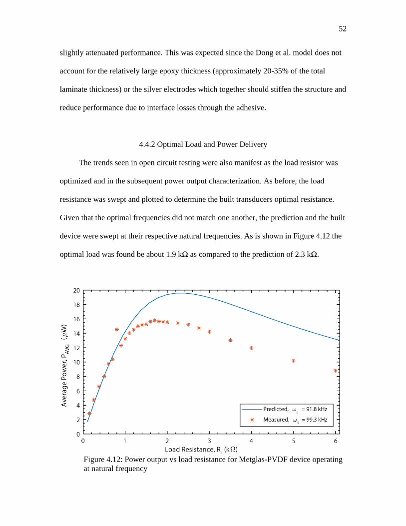
52

slightly attenuated performance. This was expected since the Dong et al. model does not

account for the relatively large epoxy thickness (approximately 20-35% of the total

laminate thickness) or the silver electrodes which together should stiffen the structure and

reduce performance due to interface losses through the adhesive.

4.4.2 Optimal Load and Power Delivery

The trends seen in open circuit testing were also manifest as the load resistor was

optimized and in the subsequent power output characterization. As before, the load

resistance was swept and plotted to determine the built transducers optimal resistance.

Given that the optimal frequencies did not match one another, the prediction and the built

device were swept at their respective natural frequencies. As is shown in Figure 4.12 the

optimal load was found be about 1.9 kΩ as compared to the prediction of 2.3 kΩ.

Figure 4.12: Power output vs load resistance for Metglas-PVDF device operating at natural frequency

53

Using the optimal load resistance of 1.9 kΩ, the power output was measured as

frequency was swept and compared to the tuned model performance. Much like the open

circuit resistance, the transducer appeared to have slightly attenuated performance from

the prediction (see Figure 4.13) but adequate power delivery given the components of the

transducer which were not taken into account.

Figure 4.13: Power output vs frequency for the Metglas-PVDF device loaded at 1.9kΩ

When compared to the Galfenol-PZT transducer, the Metglas-PVDF transducer

clearly showed better correlation to its model predictions. By looking at the model

validation globally it is evident that the model is reliable to the extent that the parameters

it is fed with are accurate. If a greater degree of accuracy were desired for these particular

54

transducer designs, a more rigorous study involving multiple structures of the same

design would be suggested as well as FEM correlation. However, given the use of this

model as an explicit equation for optimization and comparison and not for absolute

performance values, the results of this validation were sufficient for use in the design

optimization.

4.5 MME Model Validation

As was indicated previously, a parallel effort went into the derivation of the MME model.

As such, work comparable to the ME validation and involving the same test equipment

was also done to experimentally validate the transducer model. Both the model

development and validation were done by Binh Duc Truong and Dr. Shad Roundy.

Shown in Figures 4.14 and 4.15 are the experimental results of a built transducer

compared to the developed model. The transducer used for validation was a 32.55 mm

long, 3.175 mm wide and .38 mm thick bimorph made of PZT-5A with a .14 mm brass

center substrate. The magnets used were Neodymium cubes with a 3.175 mm edge

length.

Figure 4.14 shows the experimental and predicted power delivery over a frequency

sweep. Here it is visible that, at the given field level, the maximum power outputs and

operating frequencies of the model and built device match up such that their differences

are almost indistinguishable. Only by increasing the magnetic field levels, as shown in

Figure 4.15, does the model begin to slightly deviate from the experimental results.

Truong and Roundy attribute this to the fact that the built device is not perfectly

symmetrical. These results indicate that the model derived is more than adequate to be

55

used in a parameter optimization. The entirety of Truong and Roundy’s model derivation

can be seen in [47].

Figure 4.14: Experimental and modeled MME transducer power output across frequency. Figure reproduced with permission from Binh Duc Truong and Dr. Shad Roundy [47].

Figure 4.15: Experimental and modeled MME transducer power output under varying B-field at 350 Hz operating frequency. Figure reproduced with permission from Binh Duc Truong and Dr. Shad Roundy [47].

CHAPTER 5

COMPARATIVE ANALYSIS OF TRANSDUCER TYPES

Having established confidence in the analytical models describing MME and ME

transducer performance, a constrained nonlinear optimization algorithm was used to

compare transducer designs. In particular this was to be done by constraining the

optimization based on the constraints associated with operating and constructing IMD

devices.

5.1 Optimization Algorithm

The algorithm settled upon was a commonly used interior point algorithm known

as “fmincon” which is a function built into MATLAB, a numerical computing software.

Although the explicit workings of the fmincon function are proprietary, the function is

described as a gradient-based optimization method that is best suited for use with

objective functions that are continuous and have continuous derivatives[54]. This

algorithm was chosen given that the functions that predict the power output of the two

presented transducer designs met this continuity criteria.

In terms of operation, the solver takes an objective function, 𝑓𝑓(𝒙𝒙), upper and

lower bounds for inputs, 𝒙𝒙, an initial guess, 𝒙𝒙0 and iterates to find a minimizer of 𝒙𝒙

subject to linear and nonlinear constraints. For extensive information on the workings of

this function see [54], [55].

57

5.2 Optimization Constraints and Bounds

To ensure that the models were being compared under the same circumstances,

constraints were chosen to be used on all optimization runs regardless of transducer

design or material composition. The first constraints dealt with the application limitations

of the device, such as the maximum device volume, chosen to be 2mm3. Although

somewhat arbitrary, this number matches the approximate desirable size for an IMD

power source.

The next constraint was that of the applied magnetic field strength for operating the

transducers. Although much higher-level fields can physically be produced, there are

limitations to what magnitudes humans can be safely subjected. Efforts have gone into

characterizing what is known as the maximum permissible exposure (MPE) for magnetic

flux density and multiple safety standards have subsequently been published. For this

work two, common standards were chosen to bound the optimization. The first is the

Institute of Electrical and Electronics Engineers’ (IEEE) standard on magnetic MPE of

the head and torso under controlled environment conditions[56], [57]. The second is the

International Commission on Non-Ionizing Radiation Protection’s (ICNIRP) standard on

maximum occupational exposure to magnetic fields[58].

Under both standards the allowable MPE varies by frequency as is shown in Figure

5.1. By examination, it is apparent that the ICNIRP standard is generally more

conservative than the IEEE standard, which will be shown to have a large effect on

transducer performance.

58

Figure 5.1: Magnetic MPE levels for IEEE and ICNIRP Standards. Adapted from [56]–[58].

In addition to the volume and field constraints set by the IMD application of the

transducers, constraints and boundaries had to be set to ensure realistic manufacturable

optimization results. The chosen approach was to use aspect ratio constraints rather than

absolute upper bounds for almost all the optimization variables. First, aspect ratios of

200:1 were set for the length 𝑙𝑙0 and width 𝑤𝑤 to the total structure thickness, 𝑡𝑡𝑜𝑜, (magnet

thickness excluded). Additionally, the aspect ratio of the length to width (𝑙𝑙0:𝑤𝑤) was set

to a minimum of 0.1:1 and a maximum of 10:1.

It should be noted that in both the aspect ratio width refers to the entire structure

width. However, the aspect ratio’s length, 𝑙𝑙0 does not refer to the total structure length,

but the length from both transducers’ center anchors to the free edges. This means for the

ME transducer 𝑙𝑙0 = .5 ∗ 𝑙𝑙 and for the MME transducer 𝑙𝑙0 = 𝐿𝐿.

59

Like the maximum volume, these values are again somewhat arbitrary and would

in actuality vary based on exact fabrication methods. However, they do serve, as will be

shown by the optimization results, to keep the devices to dimensions that could

conceivable be built by microfabrication techniques. In addition to the aspect ratios, a

lower bound was set for the piezoelectric thickness at 10 µm with all of the other

parameters’ lower bounds being set at or near zero. The 10 µm number was chosen based

on the difficulties associated with manufacturing thin PZT. In this case the assumption

was made that the layer would be manufactured by bonding bulk PZT to a substrate then

polishing it down to the desired height. Hypothetically this method should work well at

any height but in practice, thicknesses below 10 µm are hard to achieve. The upper

bounds of the algorithm were all set at arbitrarily high values and were only decreased to

aid the solver in converging faster, in hopes they would not actually bound the

optimization results. In addition to these universally applicable constraints, design

specific constraints also had to be set.

5.2.1 ME Transducer Optimization Constraints

For the ME device, only one additional constraint was added which is based on an

assumption made by the Dong et al. model. In particular, the model makes the

assumption that the extensional strain is uniformly transferred from the MS material

through the thickness of PE material. This assumption is most valid where the laminate

length is much longer than its thickness. As the laminate length begins to approach the

magnitude of the thickness, the strain gradient becomes less and less uniform. This is due

to the bowing of the free faces normal to the length of the laminate which fundamentally

reduces the actual normal strain transferred between to the two layers. This effect is

60

demonstrated in Figure 5.2 where the normal strain gradient of the right-hand side of an

ME transducer is shown via a finite element model (FEM). Visible in this figure is the

bowing and non-uniform strain at the free face.

MS Layer

l0/tt = 11.2

PE Layer

MS Layer

Non-Uniform Strain Area Free Face

MinNormal StrainMax Figure 5.2: Normal strain gradients for right hand side of an ME device.

The plot in Figure 5.3 was generated by varying the length to width ratio (𝑙𝑙0/𝑡𝑡𝑜𝑜)

in the FEM and comparing the resulting average strain to the perfect strain assumption.

The figure indicates that as 𝑙𝑙0/𝑡𝑡𝑜𝑜 increases, the perfect strain assumption becomes more

valid. However, as the ratio decreases into the single digits and below the model

assumption rapidly begins to deteriorate. This indicates that the Dong et al. model would

over predict power delivery for structures with 𝑙𝑙0/𝑡𝑡𝑜𝑜 ratios below 10:1. To prevent this

overprediction, the lower bound for the 𝑙𝑙0/𝑡𝑡𝑜𝑜 ratio was set to be 10:1.

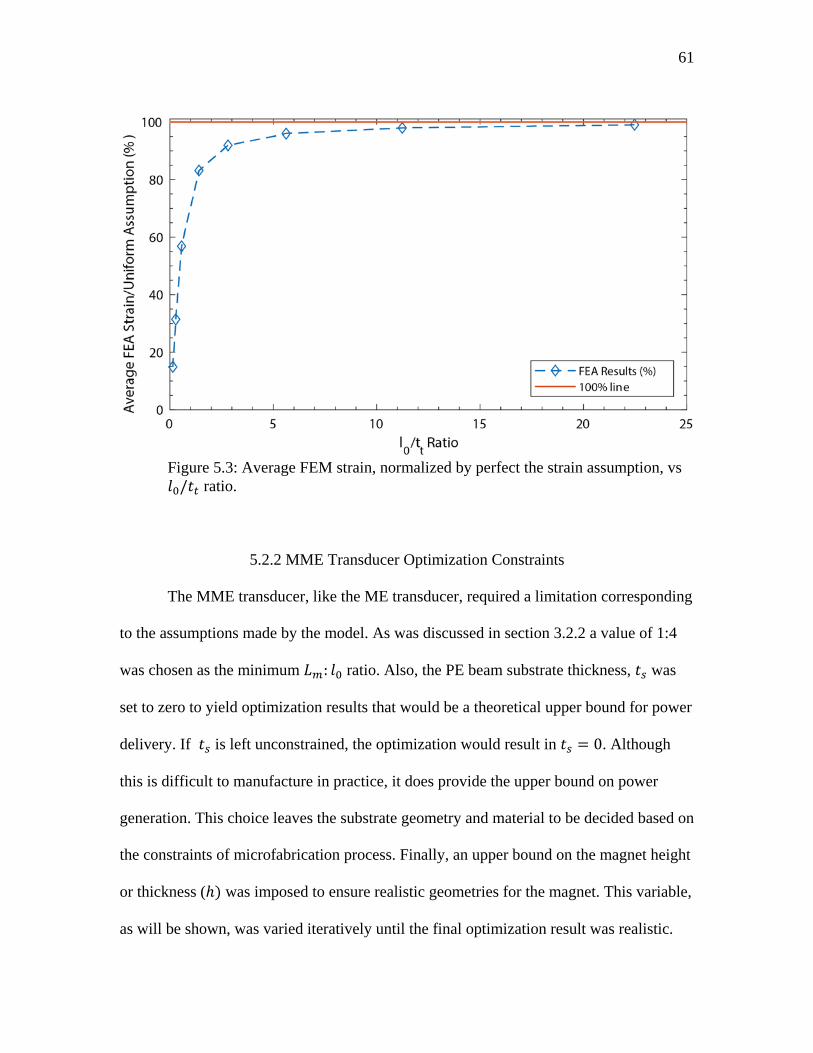
61

Figure 5.3: Average FEM strain, normalized by perfect the strain assumption, vs 𝑙𝑙0/𝑡𝑡𝑜𝑜 ratio.

5.2.2 MME Transducer Optimization Constraints

The MME transducer, like the ME transducer, required a limitation corresponding

to the assumptions made by the model. As was discussed in section 3.2.2 a value of 1:4

was chosen as the minimum 𝐿𝐿𝑚𝑚: 𝑙𝑙0 ratio. Also, the PE beam substrate thickness, 𝑡𝑡𝑠𝑠 was

set to zero to yield optimization results that would be a theoretical upper bound for power

delivery. If 𝑡𝑡𝑠𝑠 is left unconstrained, the optimization would result in 𝑡𝑡𝑠𝑠 = 0. Although

this is difficult to manufacture in practice, it does provide the upper bound on power

generation. This choice leaves the substrate geometry and material to be decided based on

the constraints of microfabrication process. Finally, an upper bound on the magnet height

or thickness (ℎ) was imposed to ensure realistic geometries for the magnet. This variable,

as will be shown, was varied iteratively until the final optimization result was realistic.

62

5.3 ME Optimization and Results

For the ME optimization, six variables were required to be varied while power

delivery was optimized: The transducer length (𝑙𝑙), width (𝑤𝑤), PE thickness (𝑡𝑡𝑝𝑝), MS

thickness (𝑡𝑡𝑚𝑚) loaded natural frequency (𝜔𝜔), and finally load resistance (𝑅𝑅𝑙𝑙). Two

material configurations were optimized, Galfenol-PZT and Metglas-PZT, using the

material properties shown in Tables 4.3 and 4.4. The mechanical quality factor was

chosen to be 48, from the average of the results witnessed during the transducer

experiments. As subsets to the configurations, each was optimized under three different

magnetic field constraints, the ICNIRP and IEEE safety standards, and a baseline

magnetic field input of 1 Oe peak at any frequency. The results of the optimization are

seen in Table 5.1.

By examination it is evident that Metglas-PZT configuration outperforms the

Galfenol-PZT configuration. Additionally, under 1 Oe or the IEEE standards both

configurations push to a short wide structure (see Figure 5.3), maximizing the allowable

𝑙𝑙0: 𝑡𝑡𝑜𝑜 ratios, minimizing the 𝑙𝑙0:𝑤𝑤 ratio, and raising the operating frequency to MHz

levels. The configurations subject to ICNIRP standard have an opposite effect going

towards a long, skinny, and thin structure maximizing the PE thickness and the 𝑙𝑙:𝑤𝑤 ratio

while maximizing the 𝑙𝑙0: 𝑡𝑡𝑜𝑜. In all cases the optimization maximized the allotted volume

of 2mm3.

Using 100 µW as the threshold of minimum power delivery to allow an IMD to

function, it is evident that the two optimized material configurations are only viable under

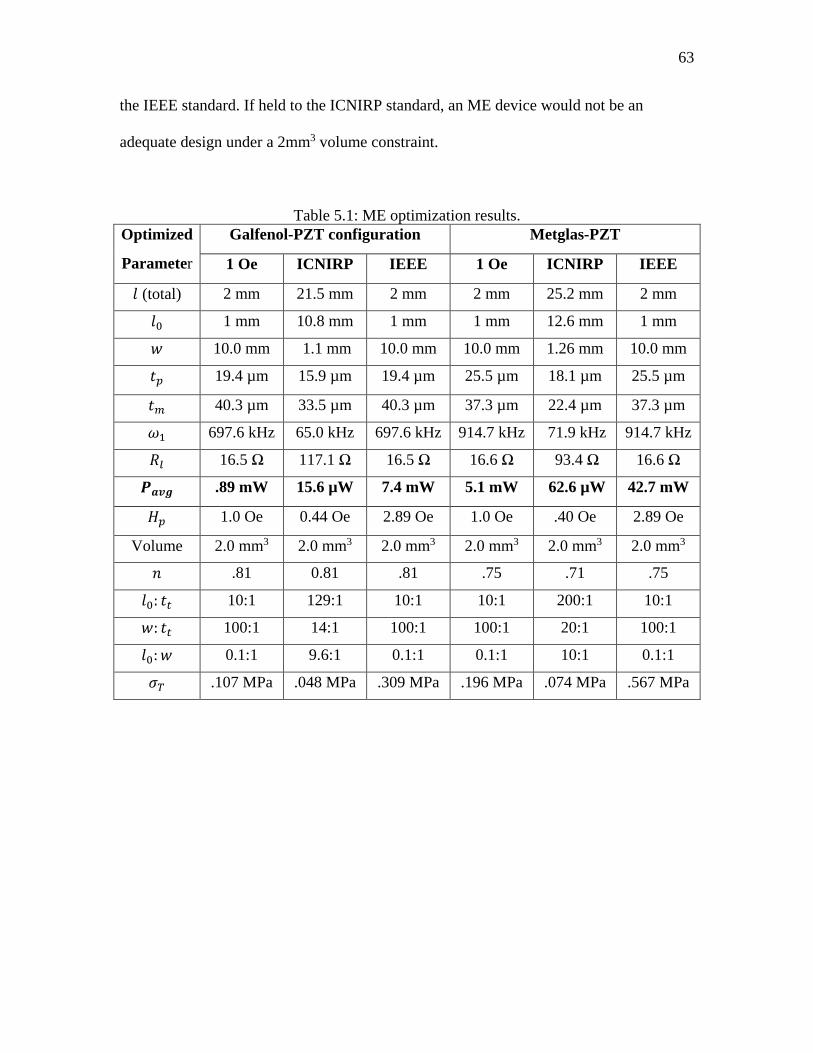
63

the IEEE standard. If held to the ICNIRP standard, an ME device would not be an

adequate design under a 2mm3 volume constraint.

Table 5.1: ME optimization results. Optimized

Parameter

Galfenol-PZT configuration Metglas-PZT

1 Oe ICNIRP IEEE 1 Oe ICNIRP IEEE

𝑙𝑙 (total) 2 mm 21.5 mm 2 mm 2 mm 25.2 mm 2 mm

𝑙𝑙0 1 mm 10.8 mm 1 mm 1 mm 12.6 mm 1 mm

𝑤𝑤 10.0 mm 1.1 mm 10.0 mm 10.0 mm 1.26 mm 10.0 mm

𝑡𝑡𝑝𝑝 19.4 µm 15.9 µm 19.4 µm 25.5 µm 18.1 µm 25.5 µm

𝑡𝑡𝑚𝑚 40.3 µm 33.5 µm 40.3 µm 37.3 µm 22.4 µm 37.3 µm

𝜔𝜔1 697.6 kHz 65.0 kHz 697.6 kHz 914.7 kHz 71.9 kHz 914.7 kHz

𝑅𝑅𝑙𝑙 16.5 Ω 117.1 Ω 16.5 Ω 16.6 Ω 93.4 Ω 16.6 Ω

𝑷𝑷𝒂𝒂𝒂𝒂𝒂𝒂 .89 mW 15.6 µW 7.4 mW 5.1 mW 62.6 µW 42.7 mW

𝐻𝐻𝑝𝑝 1.0 Oe 0.44 Oe 2.89 Oe 1.0 Oe .40 Oe 2.89 Oe

Volume 2.0 mm3 2.0 mm3 2.0 mm3 2.0 mm3 2.0 mm3 2.0 mm3

𝑛𝑛 .81 0.81 .81 .75 .71 .75

𝑙𝑙0: 𝑡𝑡𝑜𝑜 10:1 129:1 10:1 10:1 200:1 10:1

𝑤𝑤: 𝑡𝑡𝑜𝑜 100:1 14:1 100:1 100:1 20:1 100:1

𝑙𝑙0:𝑤𝑤 0.1:1 9.6:1 0.1:1 0.1:1 10:1 0.1:1

𝜎𝜎𝑇𝑇 .107 MPa .048 MPa .309 MPa .196 MPa .074 MPa .567 MPa

64

Figure 5.4: CAD representation optimized Metglas-PZT device under IEEE safety conditions. Anchor plane shown as centerline.

5.3.1 Discussion of ME Optimization Results

To show that the results of the optimizer were both realistic and useful it is

important to discuss and justify some of the results. First note that the whole numbers for

the resulting geometry were simply artifacts of the whole numbers used in the constraint

ratios and were not unexpected. Next, to explain the difference in the geometric results

between IEEE and ICNIRP standards, the situations must be examined individually.

As has been stated, IEEE device led to a short wide and thick structures operating

697.6 kHz and 914.7 kHz. For these values the magnetic field amplitude allowed by the

IEEE standard is shown to be locally constant, but for a given field magnitude the energy

contained within a field increases with frequency. This indicates that to maximize power

output under the IEEE condition, the natural frequency, 𝜔𝜔1 of the structure should also be

maximized.

It is well known that the natural frequency of a structure scales proportionally with

the structure’s stiffness and is inversely proportional to its mass. Under the constrained

volume the mass of the structure is generally constant, leaving the frequency to be

65

adjusted primarily by changing the structure’s stiffness. By using Hooke’s Law

extensional stiffness of a beam (or laminate) can be shown to be proportional to the

cross-sectional area of the beam divided by its length. Thus, if the desire is to maximize

stiffness, and subsequently 𝜔𝜔1 and the power delivered, the optimization should result in

the short, wide, and thick structure seen in the optimization. If left unconstrained, the

optimization would tend toward an infeasible structure with an infinite stiffness. These

conclusions also match that of the 1 Oe field case where the field level was also constant

across frequency.

For the ICNIRP device geometry the optimization converged on long, narrow and

thin devices operating at 65 kHz and 71.9 kHz which seems to defy the logic presented

for the IEEE case. However, the same logic can be applied to justify this result as well.

The ICNIRP standard, unlike the IEEE standard, shows a linear decline of allowable field

strength in the 65 kHz to 10 MHz frequency range. Because of the attenuation of field

strength, it is obvious that the optimization clearly worked to reduce 𝜔𝜔1 to reach the 65

kHz corner. This would indicate that ICNIRP standard’s local attenuation overwhelms

the increase in energy density due to the increase in operating frequency.

With greater power delivery levels now to be obtained at lower operating

frequencies, the same logic applied to the IEEE works to explain the ICNIRP results. To

reduce 𝜔𝜔1 the optimizer now worked to decrease stiffness by making structures that are

as long, narrow, and thin as the constraints permitted, essentially yielding the opposite

geometry of the IEEE result.

In examining these geometric results, the question was posed whether the resulting

devices were strong enough to handle the forces induced by the optimized structures or if

66

they would fracture before delivering any power. To check this, the maximum tensile

stress, 𝜎𝜎𝑇𝑇, was calculated for all of the optimal cases. The worst stress case matched that

of the highest power delivery case, the IEEE Metglas-PZT configuration. At about .567

MPa, 𝜎𝜎𝑇𝑇 was about two orders of magnitude less than PZT-5A’s tensile strength of about

50-70 MPa[59]. This indicates that all of the structure designs generated by the

optimization would be very unlikely to fracture during normal operation.

A final point of discussion concerns which magnetostrictive material is most

effective. Although both MS materials under the IEEE standard yield structures which

greatly exceed the 100 µW threshold, Metglas tends to have a higher MS coefficient and

is stiffer than Galfenol. This difference allows for greater device extension and a thicker

piezoelectric layer relative to the magnetostrictive layer thickness. Based on the

optimization, these differences equate to a Metglas device being able to deliver about six

times more power than a comparable Galfenol device. This result, taken with the

knowledge that Metglas typically requires a much lower bias field strength than Galfenol,

makes it clear that Metglas is the MS material of choice for an ME transducer being used

to power IMDs.

5.4 MME Optimization and Results

The MME optimization only required the use of five variables all related to the

geometry of the transducer: the beam length, or half the transducer length (𝐿𝐿), the beam

width (𝑤𝑤), the piezo electric thickness (𝑡𝑡𝑝𝑝), the magnet length 𝐿𝐿𝑚𝑚, and the magnet height

(ℎ). The optimal power output (𝑃𝑃𝑎𝑎𝑎𝑎𝑎𝑎), operating frequency (𝜔𝜔1), and load resistance (𝑅𝑅𝑙𝑙)

were all calculated with closed form equations.

67

Only one material configuration was optimized with PZT-5A and Neodymium 52

being used for the PE and magnet materials respectively. The material properties found in

Table 4.3 were used to represent the PZT and the properties used for the Neodymium are

shown in Table 5.2. Like the ME transducer, the configuration was optimized under the

three magnetic field conditions, 1 Oe peak, ICNIRP and IEEE. Finally, the mechanical

quality factor was set equal to 42 based on the results from Truong and Roundy.

Table 5.2: Neodymium 52 material properties [60]. Property Value

Remnant Magnetic Polarization, 𝐽𝐽𝑟𝑟 1.46 𝑇𝑇 Magnet Density, 𝜌𝜌𝑀𝑀 7500 𝑘𝑘𝑔𝑔/𝑚𝑚3

Unlike the ME optimization, the MME optimization required some iteration to

yield a manufacturable result. This was largely due to not knowing what a suitable upper

bound for the magnetic height would be. Initially a 10 mm height was set as the upper

bound to satisfy the solver inputs but not actually bound the height. Despite this large

upper bound, the results rapidly maximized the magnet height under each of the magnetic

field scenarios, even with other geometric parameters varying between the ICNIRP and

IEEE standards. The results of the optimizations done under this constraint are shown in

Table 5.3.

Examination showed that the geometries were infeasible for manufacture because

they called for a magnet that was about 50 times thicker than its length and 500 times

thicker than the PE beam to which it was to be attached. Additionally, under the IEEE

field standard, the predicted maximum bending stress, 𝜎𝜎𝐵𝐵, exceeded PZT-5A’s bending

68

strength of 140.4 MPa by over 40%. This indicated that if the structure could be built it

would fracture during operation [61].

Subsequently, the upper bound for the magnet height was reduced to 5 mm and

the optimization algorithm was run again. The corresponding results are also shown in

Table 5.3. As before, the algorithm maximized the height of the magnet up to the

imposed bound, but the results were still ultimately infeasible with the magnet still being

too thick to be integrated with the rest of the structure. Additionally, under the IEEE

condition the bending stress still exceeded the fracture strength of the beam.

69

Table 5.3: MME optimization results for 10 mm and 5 mm magnet. Optimized

Parameter

PZT Bimorph Configuration

Max 𝒉𝒉 = 10 mm

PZT Bimorph Configuration

Max 𝒉𝒉 = 5 mm

1 Oe ICNIRP IEEE 1 Oe ICNIRP IEEE

2𝐿𝐿 1.63 mm 8.00 mm 1.63 mm 3.11 mm 8.00 mm 3.11 mm

𝐿𝐿, 𝑙𝑙0 0.82 mm 4.00 mm 0.82 mm 1.56mm 4.00 mm 1.56 mm

𝑤𝑤 0.49 mm 0.40 mm 0.49 mm 0.51 mm 0.40 mm 0.51 mm

𝑡𝑡𝑝𝑝 10.0 µm 10.0 µm 10.0 µm 10.0 µm 10.0 µm 10.0 µm

𝐿𝐿𝑚𝑚 0.21 mm 0.24 mm 0.21 mm 0.39 mm 0.48 mm 0.389mm

ℎ 10.0 mm 10.0 mm 10.0 mm 5.0 mm 5.0 mm 5.0 mm

𝜔𝜔1 831 Hz 61 Hz 831 Hz 325 Hz 61 Hz 325 Hz

𝑅𝑅𝑙𝑙 2.34 MΩ 8.9 MΩ 2.34 MΩ 3.0 MΩ 8.2 MΩ 3.0 MΩ

𝑷𝑷𝒂𝒂𝒂𝒂𝒂𝒂 8.4 µW 130 µW 12.4 mW 5.9 µW 120 µW 8.7 mW

𝐻𝐻𝑝𝑝 1 Oe 5.82 Oe 38.39 Oe 1 Oe 5.56 Oe 38.39 Oe

Volume 2.0 mm3 2.0 mm3 2.0 mm3 2.0 mm3 2.0 mm3 2.0 mm3

𝐿𝐿𝑚𝑚: 𝑙𝑙0 4:1 16.5:1 4:1 4:1 8.1:1 4:1

𝑙𝑙0: 𝑡𝑡𝑜𝑜 41:1 200:1 41:1 78:1 200:1 78:1

𝑤𝑤: 𝑡𝑡𝑜𝑜 24:1 20:1 24:1 25:1 20:1 25:1

𝑙𝑙0:𝑤𝑤 1.7:1 10:1 1.7:1 3:1 10:1 3:1

𝜎𝜎𝐵𝐵 5.3 MPa 37 MPa 205 MPa 5.1 MPa 37 MPa 195 MPa

Finally, the upper bound for the optimization was reduced once more to 1 mm

which yielded the results seen in Table 5.4. As before, the magnet height was maximized

by the solver. Unlike the previous cases, the resulting geometry (which was the same for

all field cases which will be discussed in detail later) was in the realm of feasibility. In

particular this geometry was much more manufacturable given that the magnet was

almost a perfect cube with all sides being equal or close to the width of the beam. A CAD

representation of this geometry is shown in Figure 5.5.

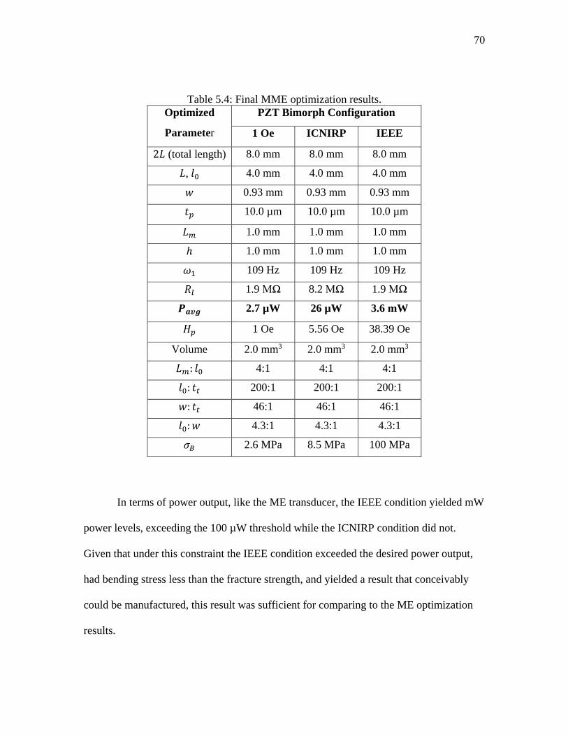
70

Table 5.4: Final MME optimization results. Optimized

Parameter

PZT Bimorph Configuration

1 Oe ICNIRP IEEE

2𝐿𝐿 (total length) 8.0 mm 8.0 mm 8.0 mm

𝐿𝐿, 𝑙𝑙0 4.0 mm 4.0 mm 4.0 mm

𝑤𝑤 0.93 mm 0.93 mm 0.93 mm

𝑡𝑡𝑝𝑝 10.0 µm 10.0 µm 10.0 µm

𝐿𝐿𝑚𝑚 1.0 mm 1.0 mm 1.0 mm

ℎ 1.0 mm 1.0 mm 1.0 mm

𝜔𝜔1 109 Hz 109 Hz 109 Hz

𝑅𝑅𝑙𝑙 1.9 MΩ 8.2 MΩ 1.9 MΩ

𝑷𝑷𝒂𝒂𝒂𝒂𝒂𝒂 2.7 µW 26 µW 3.6 mW

𝐻𝐻𝑝𝑝 1 Oe 5.56 Oe 38.39 Oe

Volume 2.0 mm3 2.0 mm3 2.0 mm3

𝐿𝐿𝑚𝑚: 𝑙𝑙0 4:1 4:1 4:1

𝑙𝑙0: 𝑡𝑡𝑜𝑜 200:1 200:1 200:1

𝑤𝑤: 𝑡𝑡𝑜𝑜 46:1 46:1 46:1

𝑙𝑙0:𝑤𝑤 4.3:1 4.3:1 4.3:1

𝜎𝜎𝐵𝐵 2.6 MPa 8.5 MPa 100 MPa

In terms of power output, like the ME transducer, the IEEE condition yielded mW

power levels, exceeding the 100 µW threshold while the ICNIRP condition did not.

Given that under this constraint the IEEE condition exceeded the desired power output,

had bending stress less than the fracture strength, and yielded a result that conceivably

could be manufactured, this result was sufficient for comparing to the ME optimization

results.

71

Figure 5.5: CAD representation optimized PZT-Brass-N52 device constrained to 1 mm magnet height. Anchor plane shown as centerline.

5.4.1 Discussion of MME Optimization Results

Because the MME transducer optimizations required some iteration, insight can be

gained about the optimization’s process and the subsequent optimal geometry. The

optimization consistently settled on the thinnest possible PE beam and attempted to

maximize the magnet size and in so doing increased the moment applied to the beam.

This would indicate that optimization was maximizing the force induced onto the beam

from moment of the permanent magnet. This was to be expected given that model

indicates that power output should scale directly with force applied (see equation 3.20).

In addition to minimizing the PE thickness and maximizing the magnet thickness,

the structure also increased the power delivery by adjusting the natural frequency of the

device. Like the ME device before, the IEEE standard was locally constant in the area of

this optimization. Table 5.3 shows that both the 10 mm and 5mm IEEE optimizations

stiffened the device by making wider and shorter cantilever beams moving the devices

72

toward more energy dense operating frequencies. Alternatively, the ICNIRP standard

was locally decreasing the allowable magnetic field with increasing frequency in the area

of MME optimization. Subsequently Table 5.3 also shows that the optimizations worked

to reduce the loaded natural frequency of the ICNIRP device by making a long, narrow

cantilever. This phenomenon is fundamentally the same as that witnessed during the ME

device optimizations.

These frequency results wouldn’t be visible, however, if the magnet height was

initially bounded to 1 mm because under this bound the optimization led to the exact

same loaded natural frequency and subsequent geometry under all magnetic field cases.

This indicated that by bounding the magnet to 1 mm the geometry was so constrained

that it essentially limited the solver to one particular natural frequency. Being skeptical of

this result, the optimization was rerun and found that indeed the ICNIRP and IEEE

standard yielded the same geometry for the 1 mm constraint up until the allowable

magnet height exceeded about 2 mm.

Despite being comfortable with the reality of results of the MME device, the

implications of the optimizations are somewhat concerning. In particular, under the best

power delivery case the magnetic field had a very large magnitude of over 38 Oe which

even at low frequencies would be difficult to generate. Additionally, the magnitude of the

operating stress is close enough to the fracture strength that the fatigue life of the device

might be very short. Finally, this optimization is a best-case scenario for power delivery

and manufacturing, in that a center substrate should likely be added to lower the bending

stress in the PE and generally make the device more durable. Such an addition would

intrinsically reduce the power delivery and make fabrication even more difficult, given

how long and thin the piezoelectric layers would be.

73

5.5 Comparison of Optimized Structures

The average power outputs and operating frequencies for each of the optimized

structures are summarized in Table 5.4. It is visible that the ME transducer delivers about

2 to 12 times the power of the MME under IEEE conditions depending on the material

configuration. Under the ICNIRP conditions the MME device delivers about two thirds

more power than the Galfenol ME device but delivers under half that of the Metglas ME

device. It is also shown that for either transducer design the IEEE limitation allows for

three orders of magnitude more power delivered than that of the ICNIRP standard for the

ME devices and 3-4 orders for the MME device. This highlights that under the 100 µW

threshold only the IEEE field standard allows for enough power delivery in a constrained

volume 2 mm3. Under this threshold it also evident that the ME laminate design is the

preferred design for powering IMDs.

In addition to the power delivery, Table 5.4 also brings to light that the AC field

magnitudes are an order of magnitude larger for the MME transducer design despite

ultimately delivering less power than the alternative. Finally, it also shows that ME

transducers operate at frequencies in the 10s of kHz to single MHz where the MME

transducers function near 100 Hz.

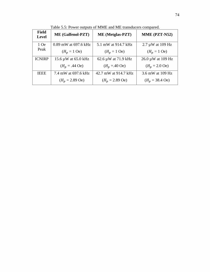
74

Table 5.5: Power outputs of MME and ME transducers compared. Field Level ME (Galfenol-PZT) ME (Metglas-PZT) MME (PZT-N52)

1 Oe Peak

0.89 mW at 697.6 kHz

(𝐻𝐻𝑝𝑝 = 1 Oe)

5.1 mW at 914.7 kHz

(𝐻𝐻𝑝𝑝 = 1 Oe)

2.7 µW at 109 Hz

(𝐻𝐻𝑝𝑝 = 1 Oe)

ICNIRP 15.6 µW at 65.0 kHz

(𝐻𝐻𝑝𝑝 = .44 Oe)

62.6 µW at 71.9 kHz

(𝐻𝐻𝑝𝑝 =.40 Oe)

26.0 µW at 109 Hz

(𝐻𝐻𝑝𝑝 = 2.0 Oe)

IEEE 7.4 mW at 697.6 kHz

(𝐻𝐻𝑝𝑝 = 2.89 Oe)

42.7 mW at 914.7 kHz

(𝐻𝐻𝑝𝑝 = 2.89 Oe)

3.6 mW at 109 Hz

(𝐻𝐻𝑝𝑝 = 38.4 Oe)

CHAPTER 6

FUTURE WORK AND CONCLUSIONS

This work constitutes a review of ME and MME transducer designs and compares

them for potential use as wireless power receivers for IMDs. This was done by

augmenting and experimentally validating an existing ME laminate model, incorporating

a tandem MME modeling effort and combining the resulting models to perform a

constrained numerical optimization. The conclusions that can be drawn from this effort as

well as possible future work are discussed in the following sections.

6.1 Conclusions

By looking purely at useful amounts power delivered, the magnetoelectric laminate

appears to be the more viable candidate for wirelessly powering a microscale IMD.

However, deeper examination tells a more intricate story. Although a somewhat simple

first order optimization, the results make clear that the extensional mode of the ME

transducer allows for a significant amount of power delivery at the cost of having to

operate at MHz frequencies which might be less desirable depending on which medical

standard is being used. Conversely the MME bending design operates at lower

frequencies where the magnet field is less susceptible to tissue absorption but ultimately

delivers about a tenth of the power. This observation, and the results of the optimization,

lead one to believe that the bending mode might be preferable to extension. However, in

76

terms of power delivery and stress to the structure, massive magnetostrictive materials

seem to be a better method of magneto-mechanical coupling than that of the moment

induced by a permanent magnet. Unfortunately, this work only compares the full

magnetoelectric performance of two transducer design and does not compare the

efficiency of the two methods of magnetic to mechanical domain transduction. In order to

definitively decide which is generally the most effective, not just when applied to IMD

applications, additional work should be done to normalize and compare permanent

magnet performance to that of magnetostrictive material.

Another important take away deals with the standard to which the transducers are

held. Clearly the IEEE standard is far less conservative than ICNIRP in that IEEE

generally allows for milliwatts of power where ICNIRP allows for microwatts. If

medically safe, the IEEE standard gives potential for either design to be conceivably

implemented. If held to the ICNIRP standard none of the devices could provide enough

power to run an IMD given that requires 100 µW.

The experiments also showed that the changes made to the Dong et al. model can

be used to predict power output of ME laminates. It can also be concluded from both the

experiments and the optimization that Metglas is a superior choice to Galfenol for MME

transducers, particularly those constrained to the IEEE and ICNIRP standards. Because

these standards prevent either Metglas or Galfenol from ever reaching saturation strain,

the driving factor becomes the rate of magnetostriction and not the absolute amount of

magnetostriction. Under the allowed field bandwidths this rate is much larger for Metglas

than for Galfenol. Additionally, as was witnessed by the results of the experimental

validation, the high permeability of Metglas makes it far easier to magnetically bias than

Galfenol. Finally, although not within the scope of this research, the fact that Metglas’

77

amorphous nature makes the magnetostriction occur anywhere in a plane as opposed to

Galfenol, which is limited to a single axis, makes Metglas a better candidate for solving

the likely alignment issues between the field and transducer.

6.2 Future Work

Based on the knowledge gained from this research, a tremendous amount of work

remains to be done to move towards the goal of powering an IMD with an oscillating

magnetic field. In particular, it seems prudent that future work would further investigate

and incorporate MS material biasing into lumped models, investigate alternative MS-PE

coupled geometries, and finally attempt to build a microscale Metglas-PZT transducer.

The need to better understand the required biasing for a given geometry was made

apparent by the mismatch in model and experimental values of the Galfenol-PZT device.

In particular it would be wise to investigate if the optimal bias field changes based on the

change in impedance of the transducer circuit, and how that subsequently effects the

magnetostrictive coefficient.

The need to examine different transducer geometries comes from the fact that there

is a large range of operating frequencies in which neither the ME nor the MME device

seems to perform well. The simplest geometry that might bridge this gap would be that of

the ME unimorph which operates in bending, unlike the ME bimorph which operates in

extension. This transducer design is not new; research has gone into adding center

substrates to unimorphs to tune and lower their operating frequency, however these

additions make the transducer more difficult to model and have not been examined from

a power delivery perspective[62]. Furthermore, other, more exotic, geometries would be

78

valuable if they were designed to utilize Metglas’ planar magnetostrictive property and

minimize sender-receiver misalignment issues.

Finally, the purpose of this research was to provide a viable design foundation for a

micro-fabricated magnetic power receiver. With this design foundation in place, work

can now move forward with manufacturing and characterization. In particular, the results

of the IEEE Metglas-PZT magnetoelectric laminate optimization reveal such an

opportunity. Although not trivial, manufacture should lead to a viable method for

wirelessly powering IMDs.

REFERENCES

[1] T. Battelino and M. Phillip, “Effect of continuous glucose monitoring on

hypoglycemia in type 1 diabetes,” Diabetes …, vol. 34, no. 4, pp. 795–800, 2011.

[2] S. Vaddiraju, “Technologies for Continuous Glucose Monitoring: Current Problems and Future Promises,” J Diabetes Sci Technol, vol. 4, no. 6, pp. 1540–1562, 2010.

[3] D. Seo, J. M. Carmena, J. M. Rabaey, E. Alon, and M. M. Maharbiz, “Neural Dust: An Ultrasonic, Low Power Solution for Chronic Brain-Machine Interfaces,” arXiv Prepr. arXiv, pp. 1307–2196, 2013.

[4] A. Arsiwala, P. Desai, and V. Patravale, “Recent advances in micro/nanoscale biomedical implants,” J. Control. Release, vol. 189, no. 2014, pp. 25–45, 2014.

[5] R. R. Harrison et al., “A low-power integrated circuit for a wireless 100-electrode neural recording system,” IEEE J. Solid-State Circuits, vol. 42, no. 1, pp. 123–133, 2007.

[6] S. H. Song, A. Kim, S. Member, B. Ziaie, and S. Member, “Omni - Directional Ultrasonic Powering for Millimeter - Scale Implantable Devices,” vol. 62, no. 11, pp. 1–8, 2015.

[7] A. Denisov and E. Yeatman, “Ultrasonic vs. Inductive Power Delivery for Miniature Biomedical Implants,” in 2010 International Conference on Body Sensor Networks, 2010, pp. 84–89.

[8] N. Tesla, “System of transmission of electrical energy.,” 645,576, 1900.

[9] N. Tesla, “The transmission of electrical energy without wires as a means for furthering peace,” Elect. World Eng., pp. 21–24, 1905.

[10] S. Y. R. Hui, Z. Wenxing, and C. K. Lee, “A critical review of recent progress in mid-range wireless power transfer,” IEEE Trans. Power Electron., vol. 29, no. 9, pp. 4500–4511, 2014.

[11] R. C. O’Handley, J. K. Huang, D. C. Bono, and J. Simon, “Improved Wireless, Transcutaneous Power Transmission for In Vivo Applications,” IEEE Sens. J., vol. 8, no. 1, pp. 57–62, 2008.

[12] H. Basaeri, D. B. Christensen, and S. Roundy, “A Review of Acoustic Power

Transfer for Bio-Medical Implants,” Smart Mater. Struct., vol. 25, no. 12, p. 123001, 2016.

[13] P. Abiri et al., “Inductively powered wireless pacing via a miniature pacemaker and remote stimulation control system,” Sci. Rep., vol. 7, no. 1, pp. 1–10, 2017.

[14] A. Ben Amar, A. B. Kouki, and H. Cao, “Power approaches for implantable medical devices,” Sensors (Switzerland), vol. 15, no. 11, pp. 28889–28914, 2015.

[15] L. Radziemski and I. R. S. Makin, “In vivo demonstration of ultrasound power delivery to charge implanted medical devices via acute and survival porcine studies,” Ultrasonics, vol. 64, pp. 1–9, 2016.

[16] Y. Rajavi, M. Taghivand, K. Aggarwal, A. Ma, and A. S. Y. Poon, “An RF-powered FDD radio for neural microimplants,” IEEE J. Solid-State Circuits, vol. 52, no. 5, pp. 1221–1229, 2017.

[17] M. Fiebig, “Revival of the magnetoelectric effect,” J. Phys. D. Appl. Phys., vol. 38, no. 8, 2005.

[18] W. C. Röntgen, “Ueber die durch Bewegung eines im homogenen electrischen Felde befindlichen Dielectricums hervorgerufene electrodynamische Kraft,” Ann. Phys., vol. 271, no. 10, pp. 264–270, 1888.

[19] I. E. Dzyaloshinskii, “On the magneto-electrical effect in antiferromagnets,” J. Sov. Phys., vol. 10, no. 3, pp. 628–629, 1960.

[20] B. D. H. Tellegen, “The gyrator, a new electric network element,” Phillips Res. Reports, vol. 3, pp. 81–101, 1948.

[21] C. W. Nan, “Magnetoelectric effect in composites of piezoelectric and piezomagnetic phases,” Phys. Rev. B, vol. 50, no. 9, pp. 6082–6088, 1994.

[22] K. H. Shin, M. Inoue, and K. I. Arai, “Preparation and properties of elastically coupled electro-magnetic elements with a bonding structure,” IEEE Trans. Magn., vol. 34, no. 4 PART 1, pp. 1324–1326, 1998.

[23] J. Ryu, A. V Carazo, K. Uchino, and H.-E. Kim, “Magnetoelectric Properties in Piezoelectric and Magnetostrictive Laminate Composites,” Jpn. J. Appl. Phys., vol. 40, pp. 4948–4951, 2001.

[24] I. D. Mayergoyz, Handbook of giant magnetostrictive materials. Elsevier, 1999.

[25] D. M. J., D. Zhangxiang, C. F. T., and F. A. B., “Magnetostrictive Devices,” Wiley Encyclopedia of Electrical and Electronics Engineering. 27-Dec-1999.

[26] “Scientists spy Galfenol’s inner beauty mark,” phys.org, 2009. [Online]. Available: https://phys.org/news/2009-03-scientists-spy-galfenol-beauty.html.

[Accessed: 01-Apr-2018].

[27] R. A. Kellog, “Development and modeling of iron-gallium alloys,” Iowa State University, 2003.

[28] Metglas Inc, “Data Sheet: Metglas 2605,” 2605SA1 Data Sheet. 2011.

[29] J. Zhai, S. Dong, Z. Xing, J. Li, and D. Viehland, “Giant magnetoelectric effect in Metglas/polyvinylidene-fluoride laminates,” Appl. Phys. Lett., vol. 89, no. 8, pp. 1–4, 2006.

[30] J. Zhai, Z. Xing, S. Dong, J. Li, and D. Viehland, “Magnetoelectric laminate composites: An overview,” J. Am. Ceram. Soc., vol. 91, no. 2, pp. 351–358, 2008.

[31] S. Dong, J. Cheng, J. F. Li, and D. Viehland, “Enhanced magnetoelectric effects in laminate composites of Terfenol-D/Pb(Zr,Ti)O 3 under resonant drive,” Appl. Phys. Lett., vol. 83, no. 23, pp. 4812–4814, 2003.

[32] S. Dong, J. F. Li, and D. Viehland, “Characterization of magnetoelectric laminate composites operated in longitudinal-transverse and transverse-transverse modes,” J. Appl. Phys., vol. 95, no. 5, pp. 2625–2630, 2004.

[33] S. Dong, J. F. Li, and D. Viehland, “Longitudinal and transverse magnetoelectric voltage coefficients of magnetostrictive/piezoelectric laminate composite: Theory,” IEEE Trans. Ultrason. Ferroelectr. Freq. Control, vol. 50, no. 10, pp. 1253–1261, 2003.

[34] S. Dong, J. F. Li, and D. Viehland, “Longitudinal and transverse magnetoelectric voltage coeffcients of magnetostrictive/ piezoelectric laminate composite: experiments,” IEEE Trans. Ultrason. Ferroelectr. Freq. Control, vol. 51, no. 7, pp. 794–799, 2004.

[35] S. Priya and D. J. Inman, Energy Harvesting Technologies. Springer US, 2008.

[36] I. Paprotny, Q. Xu, W. W. Chan, R. M. White, and P. K. Wright, “Electromechanical energy scavenging from current-carrying conductors,” IEEE Sens. J., vol. 13, no. 1, pp. 190–201, 2013.

[37] J. Han, J. Hu, Z. Wang, S. X. Wang, and J. He, “Enhanced performance of magnetoelectric energy harvester based on compound magnetic coupling effect,” J. Appl. Phys., vol. 117, no. 14, 2015.

[38] R. Jahns, R. Knoechel, and E. Quandt, “Method for measuring a magnetic field using magnetoelectric sensors,” 05-Jul-2016.

[39] S. Marauska, R. Jahns, H. Greve, E. Quandt, R. Kn, and B. Wagner, “MEMS magnetic field sensor based on magnetoelectric composites,” Micromechanics and Microengineering, vol. 22, 2012.

[40] S. Marauska et al., “Highly sensitive wafer-level packaged MEMS magnetic field sensor based on magnetoelectric composites,” Sensors Actuators A Phys., vol. 189, pp. 321–327, 2013.

[41] T. Nan, Y. Hui, M. Rinaldi, and N. X. Sun, “Self-biased 215MHz magnetoelectric NEMS resonator for ultra-sensitive DC magnetic field detection,” Sci. Rep., vol. 3, p. 1985, 2013.

[42] C. W. Nan, M. I. Bichurin, S. Dong, D. Viehland, and G. Srinivasan, “Multiferroic magnetoelectric composites: Historical perspective, status, and future directions,” J. Appl. Phys., vol. 103, no. 3, 2008.

[43] M. Paluszek et al., “Magnetoelectric composites for medical application,” in Composite Magnetoelectrics, Elsevier, 2015, pp. 297–327.

[44] G. Yang, H. Talleb, A. Gensbittel, and Z. Ren, “FEM Modeling of a Magnetoelectric Transducer for Autonomous Micro Sensors in Medical Application,” Sens. Imaging, vol. 16, no. 1, pp. 1–10, 2015.

[45] C. Shuo, C. Clemens, and A. D. P., “Electrodynamic Vibrational Energy Harvesting,” in Micro Energy Harvesting, 1st ed., D. Briand, E. M. Yeatman, and S. Roundy, Eds. 2015, pp. 175–197.

[46] Y. Zhou, S. Chul Yang, D. J. Apo, D. Maurya, and S. Priya, “Tunable self-biased magnetoelectric response in homogenous laminates,” Appl. Phys. Lett., vol. 101, no. 23, 2012.

[47] B. D. Truong and S. Roundy, “Model Validation and Investigation on the Efficiency of Wireless Power Transfer System with Middle Clamped Piezoelectric Reciever,” unpublished.

[48] J. J. Abbott, “Parametric design of tri-axial nested Helmholtz coils,” Rev. Sci. Instrum., vol. 86, no. 5, pp. 1–10, 2015.

[49] L. Bian, Y. Wen, P. Li, Q. Gao, and M. Zheng, “Magnetoelectric transducer with high quality factor for wireless power receiving,” Sensors Actuators, A Phys., vol. 150, no. 2, pp. 207–211, 2009.

[50] PSI-5A4E Piezoceramic Plates and Sheets. Woburn: Systems, Piezo, 2011.

[51] E. Summers, “Galfenol – a New Class of Magnetostrictive Materials.”

[52] Measurement Specialties, Piezo Film Sensors Technical Manual, no. March. 2006.

[53] E. Freeman et al., “Improving the magnetoelectric performance of Metglas/PZT laminates by annealing in a magnetic field,” Smart Mater. Struct., vol. 26, no. 8, p. 85038, 2017.

[54] MathWorks, “fmincon,” 2018. [Online]. Available: https://www.mathworks.com/help/optim/ug/fmincon.html#busp5fq-6. [Accessed: 11-May-2018].

[55] MathWork, “Constrained Nonlinear Optimization Algorithms,” 2018. [Online]. Available: https://www.mathworks.com/help/optim/ug/constrained-nonlinear-optimization-algorithms.html#brnox01. [Accessed: 11-May-2018].

[56] IEEE International Committee on Electromagnetic Safety, IEEE Standard for Safety Levels With Respect to Human Exposure to Radio Frequency Electromagnetic Fields, 3 kHz to 300 GHz. New York, NY: The Institute of Electrical and Electronics Engineers, Inc., 2006.

[57] IEEE Standards Coordinating Committee, IEEE Standard for Safety Levels with Respect to Human Exposure to Electromagnetic Fields, 0–3 kHz. New York, NY: The Institute of Electrical and Electronics Engineers, Inc., 2003.

[58] International Commission on Non-Ionizing Radiaton Protection, “ICNIRP Guidelines for Limiting Exposure To Time‐Varying Electric, Magnetic, and Electromagnetic Fields (up to 300 GHz),” Health Phys., vol. 74, no. (4), p. 494‐522;, 1998.

[59] X. Kornmann and C. Huber, “Microstructure and mechanical properties of PZT fibres,” J. Eur. Ceram. Soc., vol. 24, no. 7, pp. 1987–1991, 2004.

[60] K&J Magnetics, “Specification.” [Online]. Available: https://www.kjmagnetics.com/specs.asp. [Accessed: 05-May-2018].

[61] S. R. Anton, A. Erturk, and D. J. Inman, “Bending strength of piezoelectric ceramics and single crystals for multifunctional load-bearing applications,” IEEE Trans. Ultrason. Ferroelectr. Freq. Control, vol. 59, no. 6, pp. 1085–1092, 2012.

[62] Z. Xing, S. Dong, J. Zhai, L. Yan, J. Li, and D. Viehland, “Resonant bending mode of Terfenol-D∕steel∕Pb(Zr,Ti)O3 magnetoelectric laminate composites,” Appl. Phys. Lett., vol. 89, no. 11, p. 112911, 2006.