A Comparison of Common Methods forOptimal Well Placement

Jeremy J. MintonSupervised by: Associate Professor Rosalind Archer

Department of Engineering Science, Faculty of Engineering, University of Auckland, New Zealand

AbstractThe well placement problem is challenging due to the non-linear, discrete and often

multi-modal objective function. This is complicated by computationally expensive func-tion evaluations from reservoir simulation, typically producing no gradient information.Heuristics for automated optimisation have been proposed over the past 20 years withminimal comparison or benchmarking of performance. This paper presents a comparisonof common methods, including genetic algorithms, simulated annealing, particle swarmoptimisation and variants of the hill climbing algorithms. These algorithms were testedin the context of locating a single production or injection well in two reservoir cases. Forthis class of problem, the genetic algorithm produced good results after 100 evaluations.The particle swarm method performed only slightly worse but was able to improve con-siderably with the use of ‘educated guesses’ seeding it’s initialisation. For this reason theparticle swarm optimiser is arguably the better method for industrial implementation assome idea of optimality would exist through intuition and experience. A recommend-ation for further development is the investigation of objective function approximationsfor initialisation seeding as well as sequentially combining algorithms, such as particleswarm and simulated annealing, to find a combination of explorative then exploitativesearching. The validity of these results are limited, however, due to the small samplesize and to single well problems. In fact, some findings were contradictory to previouslypublished guidelines which illustrates the need for this type of comparison: understandingan algorithm’s performance under given conditions is necessary in leveraging its benefits,particularly with such demanding problems such as well placement.

Keywords:well placement, algorithm comparison, heuristics, particle swarm optimisation, genetic al-gorithm, simulated annealing, hill climbing

Email:jmin040@aucklanduni.ac.nz (Jeremy Minton)

122

1 Introduction

Selecting optimal well sites is a valuable problem to solve; maximising oil recovery increases oil reserves and min-imising costs improves profitability. Unfortunately, the non-linear and multi-modal response of well locations andthe discrete nature of most decision variables through the discretisation of the reservoir, make this a challengingoptimisation problem for deterministic searches. Furthermore, the function evaluation involves computationalsimulation of the fluid flow within the reservoir; typically called reservoir simulation. The high computationalcost of performing these reservoir simulations increases the demand for an algorithm to find optimality with thefewest function evaluations.

Consequently, since 1995, research has been focused on developing heuristics to rapidly solve reservoir simu-lation models for near optimality (Aanonsen et al., 1995; Beckner and Song, 1995). This topic has been gainingpopularity as computer processing speed has improved the feasibility of these investigations.

Unfortunately, the problem is dependent on properties of the particular reservoir: heterogeneity will increasethe noise in the objective function and produce larger and more local optima; the number of wells to be placedcan be introduced as a control variable which creates a stepped objective function; similarly, a variable numberof lateral wells or completion intervals can be optimised. Each subsequent layer of complexity makes the problemmore difficult to solve and alters the efficiency of any algorithm configuration used.

The high computational cost of reservoir simulation implies that the complexity of the algorithm is negligiblecompared to function evaluations. Consequently, many methods have been proposed.

1.1 Published Algorithms

Interpolation methods were one of the first methods applied to the well placement problem, having been adaptedfrom the history matching problem. Examples of the surface approximation techniques used include Kriging, leastsquares and regression surfaces (Pan and Horne, 1998; Aanonsen et al., 1995).

Simulated annealing, is a meta-heuristic that is based on the annealing process in metallurgy. It was, also,one of the first published methods, applied to the well placement problem by Beckner and Song (1995).

Evolutionary algorithms use a process of survival of the fittest: better solutions have a higher probability of‘mating’ and hence their characteristics are more likely to persist into later iterations. Evolutionary strategiesare currently the most popular methods with 2,260 results of 8,840 found in the OnePetro database on ‘wellplacement optimisation’ also containing the term “genetic” or “evolution”. Some relevant papers for the interestedreader include Montes et al. (2001); Tupac et al. (2007); Morales et al. (2011); Ding (2008).

Particle swarm optimisation (PSO) was originally designed by Kennedy and Eberhart (1995) as a continuousnon-linear function optimiser and has had a range of developments and applications as summarised in Poli et al.(2007). It has been applied to the well placement problem in three publications; Onwunalu and Durlofsky (2009a),Onwunalu and Durlofsky (2009b) and Ciaurri et al. (2011).

A number of publications have been made regarding variations of the descent algorithms. These includederivative free hill climbing such as stochastic directions, pattern searches, direct searches as well as derivativemethods like finite differences or adjoint gradient estimation methods (Bangerth et al., 2006; Onwunalu andDurlofsky, 2009b; Zandvliet et al., 2008; Sarma and Chen, 2008).

An assortment of other less common algorithms have also been posed. Wang et al. (2007) presents a novelapproach in which flow rates of wells at every grid point are optimised and wells are eliminated as their flow ratedrops to zero. A method to optimise lateral wells based on quality maps, a guide to regions of high productionpotential, is presented in Nakajima and Schiozer (2003). Lo et al. (1995) developed a linear forecasting modelto harness linear programming techniques. Finally, Ciaurri et al. (2011) identifies asynchronous parallel patternsearch, implicit filtering, dividing rectangles and some statistical emulation methods.

Additionally, many combination and hybrid methods have also been examined which combine different al-gorithms to exploit the high performing behaviours of each. Bittencourt and Horne (1997); Zangl et al. (2006);Badru and Kabir (2003); Guyaguler et al. (2002) are a few examples for the interested reader.

This is by no means an exhaustive list.

1.2 Algorithm Comparison

Despite the great disparity in the number of function evaluations required, ranging from tens to thousands in thepreviously cited papers, (Bangerth et al., 2006) is one of the few studies that compares algorithms: simultaneousperturbation stochastic approximation, finite difference gradient, very fast simulated annealing, Nelder-Meadsimplex and a genetic algorithm in this case. Performing this style of comparison with a sufficiently comprehensiveselection of algorithms on case studies representative of industrial problems would fill an apparent gap in publishedliterature. Through better understanding the behaviour and performance, the improvement and even developmentof new, novel algorithms could be directed.

To this end, this study investigates the application of four optimisation algorithms in two well placementoptimisation problems. Due to computational restraints the problems were restricted to locating a single vertical

123

well, defined by two surface indices and the bottommost perforation depth. This allowed an exhaustive search tobe performed so multiple trials could be completed for statistical validity. The algorithms tested were the descentmethod, simulated annealing, genetic algorithm and particle swarm optimisation.

2 Methodology

The algorithms compared in this study were tested optimising the location and depth of a single well in onesynthetic and one realistic reservoir model. The problem formulation and test cases follow in this section. Thealgorithms, described in the next section, were implemented as constrained optimisation algorithms and eachparameter set was used to optimise each well placement problem 200 times. These repetitions are to account forthe algorithm’s stochastic behaviour.

2.0.1 Parameter Selection

The performance of an algorithm in a given context will depend on the balance of exploitative and explorativebehaviours. Identifying appropriate control parameters achieves this correct balance, however, this is not a trivialproblem and they are rarely transferable between functions. Unfortunately, computational limits prevented anexhaustive search or optimisation of these parameters hence those identified as generally successful in literaturewere used. Some variations were also tested for assessing performance sensitivity. These are detailed withappropriate citations in Section 3.

2.0.2 Seeded Initialisation

It was identified in Zandvliet et al. (2008) that hill climbing has the advantage that it will improve at everyiteration until the local optimum is found, whereas meta-heuristics may undergo numerous iterations withoutmaking any improvement. This suggests an algorithm’s ability to utilise information from a previous iterationvaries and hence it’s ability to utilise information from intelligently selected initialisation points. The reservoirsimulation process is not a black box; quickly calculable approximations and experientially based guesses containlarge amounts of information about the system. Although not acceptable for optimisation, such approximationshave merit by eliminating the obviously poor regions of the reservoir from the search space. Hence, effective useof ‘a priori’ knowledge would make the process attractive in the industrial environment; such an algorithm couldbe readily adopted into commercial use as a final tuning step in the conventional planning process.

This is tested in a second round of experiments by substituting otherwise randomly generated initial solutionswith initial ‘guesses’ of the solution. The maximum of some function, based on some quickly attainable estimateof the objective function, is used, where one is randomly chosen when multiple maxima exist; these estimatedsolutions are referred to as optimal solution approximations or just approximations in this paper.

Once all approximations have been used to generate points, random selection continues. This means for apopulation algorithm, the first number of individuals are generated from approximations and the remaining arerandom and for single-point methods the first number of restarts are guided by approximations before restartingrandomly.

These approximations, in priority for use, are:

1. Well performance index (WPI) The well performance index from a simulation of a very low productionrate well at every cell for a single time-step.

2. Permeability The input permeability for each cell of the reservoir.

3. Porosity The input porosity for each cell of the reservoir.

4. Cell Thickness The vertical dimension of each cell in the reservoir.

5. Cell Depth The depth of the top of each cell in the reservoir.

6. Net to gross The input net to gross (refer to glossary) of each cell in the reservoir.

Each estimated function surface, from which the optimal solution approximations was selected, is comparedto the objective function surfaces in Appendix B.

2.1 Problem Formulation

The optimisation problem used in this paper is:

Decision VariablesGrid block co-ordinates of the well head.Layer index of the lower perforation limit (only considered for the three dimensional case).

124

Objective Functions Two objective functions were considered independently.Maximise cumulative oil production (COP) of the field or,maximise net present value (NPV) of the field.

ConstraintsBoundary constraints - wells must be located within the reservoir simulation model.

2.1.1 Objective Function Evaluation

NPV is calculated using the formulation provided in Onwunalu and Durlofsky (2009b), reproduced here forconvenience.

NPV =

T∑t=1

CFt

(1 + r)t− Ccapex,

where r is the rate of return, T is the set of time intervals, CFt is cash flow in the time period t and capitalexpenditure, Ccapex, is the cost of any development work and is defined as,

Ccapex =

Nwell∑w=1

Csurface + CdrillLshaft,

where Nwell is the number of wells to be drilled, C is the cost of the superscript and L is the well depth infeet.

The cash flow term is revenue minus expenses,

CFt = poQot + pgQg

t − CwpQwpt − CwiQwi

t ,

where p is the price of oil or gas, C is the cost of water production or water injection and Q denotes theproduction or injection rates of each fluid during the denoted time interval.

The values used in these calculations are included in Table 1. For simplicity many financial considerations

Table 1: Values Used in the NPV Calculation

Term Valuer 10%

Csurface $5,000,000 per WellCdrill $0 per footpo $22 per stock tank barrelpg $1.5 per thousand cubic feetCwp $1 per stock tank barrelCwi $1 per stock tank barrel

are omitted including the cost of drilling, cost forecasting, location dependent costs or more complex capitalexpenditure models. A more sophisticated class of model may improve accuracy but should not overly influencethe response surface.

2.2 Test Cases

Using the ‘ECLIPSE’ reservoir simulator (ECLIPSE, 2009), an exhaustive search of the location and depth ofone well over the reservoir models considered was performed, holding all other properties constant including celllayout, cell parameters and existing well configurations. This produced a response surface that shortened functionevaluations to a single look-up operation. The response surfaces are presented in Appendix A.

2.2.1 Synthetic Reservoir

The synthetic reservoir used was ‘SPE9’. After completion of a large study by the Society for Petroleum Engineers,this model was made available with the ‘ECLIPSE’ simulator. It is synthesised to be representative of a northsea formation, with uniform cell thickness and porosity by layer ranging from 8 to 100 feet and 0.08 to 0.157respectively. Each cell’s permeability is horizontally isotropic with the vertical permeability roughly one hundredthof this value; values range from less than 1 milli-Darcy to several Darcy throughout the reservoir. There is a water

125

Figure 1: Three dimensional view of the synthetic reservoir showing the oil saturation; the blue and red coloursindicating high and low saturation respectively.

leg, the low oil saturation at the bottom edge of the reservoir in Figure 1, but no gas cap. The model contains24× 25× 15 cells.

The model was used to locate one new production well amongst 26 existing producers and one water injectionwell. The perforation interval began from the second layer, limiting the three-dimensional optimisation to 14layers. For the two dimensional trials the completion depth was taken as the tenth layer. Oil production wasfound to correlate with the oil saturation at the location of the new producer.

2.2.2 Real-World Reservoir

The realistic reservoir used contains 54× 55× 5 cells. It is a black-oil model with uniform porosity of 0.26 in thefirst four layers and 0.15 in the bottom; uniform permeability of 20mD except a zone at 70mD near well ‘N1’ andanother of 2mD about well ‘N8’. The structure of the reservoir, initial oil saturation and location of six existingproduction wells, is displayed in Figure 2.

Figure 2: Three dimensional view of the realistic reservoir showing the oil saturation; the blue and red coloursindicating high and low saturation respectively.

126

The location and perforation intervals of one water injection well was optimised. Three-dimensional optim-isation occurred over all five layers and the completion depth was taken as the bottom layer for two-dimensionaltrials. Optimal COP and NPV occurs when the injection well is placed in the gas cap to displace oil downwardsto the production wells.

2.3 Performance Measures

Clerc (2011) proposes that a mean alone is insufficient to measure performance as a single high performing run issufficient for a solution. Consequently, plots of average value found against unique function evaluations are used.One standard deviation error bars are included for only some cases to improve clarity. In addition to these plots,three performance measures are considered, based on those presented in Bangerth et al. (2006).

Effectiveness Effectiveness is a simple measure of performance and is the mean value between trials of the bestsolution found as a percent of the global optimum or,

f̄ =1

N

N∑i=1

f(p̂i)

f(p∗) ,

where f(p) is the value of solution p, p∗ is the globally optimum solution, p̂i is the best solution found intrial i and N is the number of trials for each algorithm configuration.

Efficiency Efficiency indicates how quickly the algorithm reaches a level of performance using the number ofunique evaluations required to find a solution of at least 98% the best solution value found, averaged betweentrials or

L̄ =1

N

N∑i=1

L98i

M, (1)

where, additionally, L98i is the number of unique function evaluations required to find solution q such that

f(q) ≤ 0.98f(p̂i) for trial i (for minimisation) and M is the total number of function evaluations per trial.

Reliability Reliability indicates the expected minimum performance for a given number of optimisation runs bytaking the effectiveness of a certain percentile of trials or,

φk =f(p̂k%)

f(p∗) , (2)

where, p̂k% is the lowest value required to reach the top kth percentile of trials when ranked by their bestsolution.

All objective functions have been normalised to range from zero to one and only unique function evaluationsare counted.

3 Algorithm Configuration

Four algorithms were implemented for testing, including assorted hill climbing methods, simulated annealing,genetic algorithm and particle swarm optimisation. A random search was also implemented and is included inresults for comparison. Each implementation is briefly described here.

3.1 Hill Climbing Algorithm

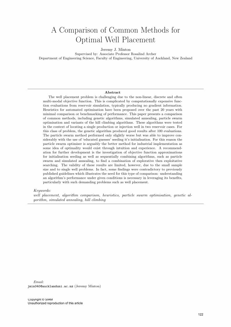
This algorithm was implemented in Matlab (MATLAB, 2010) using three search patterns and three test-distance/step-size methods based on developments in Spall (1992). The search patterns include searching all neighbouring points;searching at random, then moving as soon as a better solution is found; and searching based on the directionof the last step: opposite directions then orthogonal directions. The three stepping methods are presented inTable 2 where ck and ak are test distance and nominal step-size, initialised to half the minimum domain width;alpha = 0.602 and gamma = 0.101 are constants to control how quickly the search distance contracts; k is aniteration counter; and ∆f

ckis a linear gradient estimate of the current location using the test location. Further

details of the SPSA test-distance/step-size can be found in Bangerth et al. (2006).A penalty method, setting an infeasible solution’s objective function to Matlab’s ‘inf’ value is used to prevent

the search leaving the feasible region. A random restart was implemented once the algorithm reached localoptimality.

127

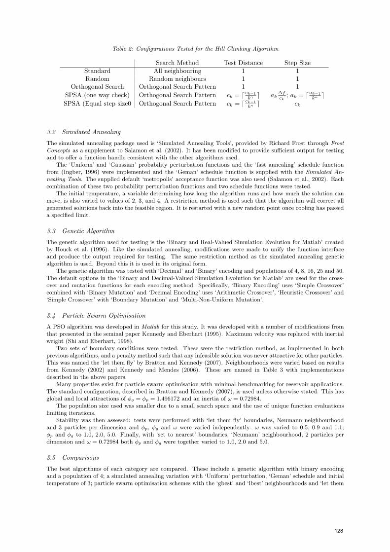
Table 2: Configurations Tested for the Hill Climbing Algorithm

Search Method Test Distance Step SizeStandard All neighbouring 1 1Random Random neighbours 1 1

Orthogonal Search Orthogonal Search Pattern 1 1SPSA (one way check) Orthogonal Search Pattern ck = ⌈ ck−1

kγ ⌉ ak∆fck

; ak = ⌈ak−1

kα ⌉SPSA (Equal step size0 Orthogonal Search Pattern ck = ⌈ ck−1

kγ ⌉ ck

3.2 Simulated Annealing

The simulated annealing package used is ‘Simulated Annealing Tools’, provided by Richard Frost through FrostConcepts as a supplement to Salamon et al. (2002). It has been modified to provide sufficient output for testingand to offer a function handle consistent with the other algorithms used.

The ‘Uniform’ and ‘Gaussian’ probability perturbation functions and the ‘fast annealing’ schedule functionfrom (Ingber, 1996) were implemented and the ‘Geman’ schedule function is supplied with the Simulated An-nealing Tools. The supplied default ‘metropolis’ acceptance function was also used (Salamon et al., 2002). Eachcombination of these two probability perturbation functions and two schedule functions were tested.

The initial temperature, a variable determining how long the algorithm runs and how much the solution canmove, is also varied to values of 2, 3, and 4. A restriction method is used such that the algorithm will correct allgenerated solutions back into the feasible region. It is restarted with a new random point once cooling has passeda specified limit.

3.3 Genetic Algorithm

The genetic algorithm used for testing is the ‘Binary and Real-Valued Simulation Evolution for Matlab’ createdby Houck et al. (1996). Like the simulated annealing, modifications were made to unify the function interfaceand produce the output required for testing. The same restriction method as the simulated annealing geneticalgorithm is used. Beyond this it is used in its original form.

The genetic algorithm was tested with ‘Decimal’ and ‘Binary’ encoding and populations of 4, 8, 16, 25 and 50.The default options in the ‘Binary and Decimal-Valued Simulation Evolution for Matlab’ are used for the cross-over and mutation functions for each encoding method. Specifically, ‘Binary Encoding’ uses ‘Simple Crossover’combined with ‘Binary Mutation’ and ‘Decimal Encoding’ uses ‘Arithmetic Crossover’, ‘Heuristic Crossover’ and‘Simple Crossover’ with ‘Boundary Mutation’ and ‘Multi-Non-Uniform Mutation’.

3.4 Particle Swarm Optimisation

A PSO algorithm was developed in Matlab for this study. It was developed with a number of modifications fromthat presented in the seminal paper Kennedy and Eberhart (1995). Maximum velocity was replaced with inertialweight (Shi and Eberhart, 1998).

Two sets of boundary conditions were tested. These were the restriction method, as implemented in bothprevious algorithms, and a penalty method such that any infeasible solution was never attractive for other particles.This was named the ‘let them fly’ by Bratton and Kennedy (2007). Neighbourhoods were varied based on resultsfrom Kennedy (2002) and Kennedy and Mendes (2006). These are named in Table 3 with implementationsdescribed in the above papers.

Many properties exist for particle swarm optimisation with minimal benchmarking for reservoir applications.The standard configuration, described in Bratton and Kennedy (2007), is used unless otherwise stated. This hasglobal and local attractions of ϕg = ϕp = 1.496172 and an inertia of ω = 0.72984.

The population size used was smaller due to a small search space and the use of unique function evaluationslimiting iterations.

Stability was then assessed: tests were performed with ‘let them fly’ boundaries, Neumann neighbourhoodand 3 particles per dimension and ϕp, ϕg and ω were varied independently. ω was varied to 0.5, 0.9 and 1.1;ϕp and ϕg to 1.0, 2.0, 5.0. Finally, with ‘set to nearest’ boundaries, ‘Neumann’ neighbourhood, 2 particles perdimension and ω = 0.72984 both ϕp and ϕg were together varied to 1.0, 2.0 and 5.0.

3.5 Comparisons

The best algorithms of each category are compared. These include a genetic algorithm with binary encodingand a population of 4; a simulated annealing variation with ‘Uniform’ perturbation, ‘Geman’ schedule and initialtemperature of 3; particle swarm optimisation schemes with the ‘gbest’ and ‘lbest’ neighbourhoods and ‘let them

128

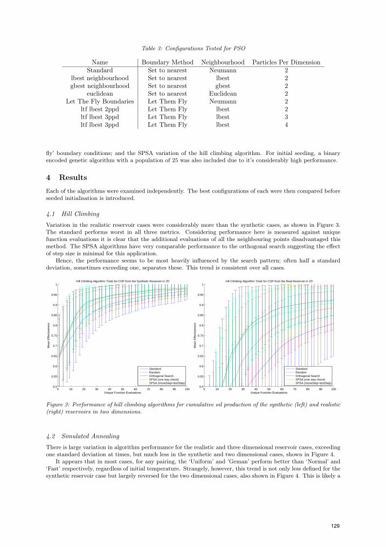
Table 3: Configurations Tested for PSO

Name Boundary Method Neighbourhood Particles Per DimensionStandard Set to nearest Neumann 2

lbest neighbourhood Set to nearest lbest 2gbest neighbourhood Set to nearest gbest 2

euclidean Set to nearest Euclidean 2Let The Fly Boundaries Let Them Fly Neumann 2

ltf lbest 2ppd Let Them Fly lbest 2ltf lbest 3ppd Let Them Fly lbest 3ltf lbest 3ppd Let Them Fly lbest 4

fly’ boundary conditions; and the SPSA variation of the hill climbing algorithm. For initial seeding, a binaryencoded genetic algorithm with a population of 25 was also included due to it’s considerably high performance.

4 Results

Each of the algorithms were examined independently. The best configurations of each were then compared beforeseeded initialisation is introduced.

4.1 Hill Climbing

Variation in the realistic reservoir cases were considerably more than the synthetic cases, as shown in Figure 3.The standard performs worst in all three metrics. Considering performance here is measured against uniquefunction evaluations it is clear that the additional evaluations of all the neighbouring points disadvantaged thismethod. The SPSA algorithms have very comparable performance to the orthogonal search suggesting the effectof step size is minimal for this application.

Hence, the performance seems to be most heavily influenced by the search pattern; often half a standarddeviation, sometimes exceeding one, separates these. This trend is consistent over all cases.

0 10 20 30 40 50 60 70 80 90 1000.5

0.55

0.6

0.65

0.7

0.75

0.8

0.85

0.9

0.95

1Hill Climbing Algorithm Trials for COP from the Synthetic Reservoir in 2D

Unique Function Evaluations

Mea

n E

ffect

iven

ess

StandardRandomOrthogonal SearchSPSA (one way check)SPSA (moveStep=testStep)

0 10 20 30 40 50 60 70 80 90 1000.5

0.55

0.6

0.65

0.7

0.75

0.8

0.85

0.9

0.95

1Hill Climbing Algorithm Trials for COP from the Real Reservoir in 2D

Unique Function Evaluations

Mea

n E

ffect

iven

ess

StandardRandomOrthogonal SearchSPSA (one way check)SPSA (moveStep=testStep)

Figure 3: Performance of hill climbing algorithms for cumulative oil production of the synthetic (left) and realistic(right) reservoirs in two dimensions.

4.2 Simulated Annealing

There is large variation in algorithm performance for the realistic and three dimensional reservoir cases, exceedingone standard deviation at times, but much less in the synthetic and two dimensional cases, shown in Figure 4.

It appears that in most cases, for any pairing, the ‘Uniform’ and ’Geman’ perform better than ‘Normal’ and‘Fast’ respectively, regardless of initial temperature. Strangely, however, this trend is not only less defined for thesynthetic reservoir case but largely reversed for the two dimensional cases, also shown in Figure 4. This is likely a

129

consequence of the modality of each problem and suggests that the larger perturbations and more frequent restartof ‘Normal’ and ‘Fast’ annealing are better able to overcome local optima.

0 10 20 30 40 50 60 70 80 90 1000.5

0.55

0.6

0.65

0.7

0.75

0.8

0.85

0.9

0.95

1Simulated Annealing Trials for COP from the Synthetic Reservoir in 2D

Unique Function Evaluations

Mea

n E

ffect

iven

ess

Uniform,Geman,Tinit=3Normal,Geman,Tinit=3Unifrom,FastAnnealing,Tinit=3Normal,FastAnnealing,Tinit=3Uniform,Geman,Tinit=2Normal,Geman,Tinit=2Unifrom,FastAnnealing,Tinit=2Normal,FastAnnealing,Tinit=2Uniform,Geman,Tinit=4Normal,Geman,Tinit=4Unifrom,FastAnnealing,Tinit=4Normal,FastAnnealing,Tinit=4

0 10 20 30 40 50 60 70 80 90 1000.5

0.55

0.6

0.65

0.7

0.75

0.8

0.85

0.9

0.95

1Simulated Annealing Trials for COP from the Real Reservoir in 3D

Unique Function Evaluations

Mea

n E

ffect

iven

ess

Uniform,Geman,Tinit=3Normal,Geman,Tinit=3Unifrom,FastAnnealing,Tinit=3Normal,FastAnnealing,Tinit=3Uniform,Geman,Tinit=2Normal,Geman,Tinit=2Unifrom,FastAnnealing,Tinit=2Normal,FastAnnealing,Tinit=2Uniform,Geman,Tinit=4Normal,Geman,Tinit=4Unifrom,FastAnnealing,Tinit=4Normal,FastAnnealing,Tinit=4

Figure 4: Performance of simulated annealing algorithms for cumulative oil production of the synthetic (left) andrealistic (right) reservoirs in three dimensions.

4.3 Genetic Algorithm

The difference in performance between configurations is within one standard deviation in all but two cases.Within these limits, there is a consistent trend in which the larger populations generally produce poorer

performance and the binary encoding also appears less effective. One clear example is the cumulative oil productionfor the three dimensional realistic reservoir case; these results are presented in Figure 5 where the two trends areillustrated in the left and right plots respectively.

Overlaying these results the population size is more influential of the performance the encoding used.The smaller populations can, however, perform worse in early time. As the genetic algorithm is initialised

with random solutions, this implies that the smaller populations perform worse than a random search despiteutilising information about the objective function after each iteration.

0 10 20 30 40 50 60 70 80 90 1000.5

0.55

0.6

0.65

0.7

0.75

0.8

0.85

0.9

0.95

1Genetic Algorithm Trials for COP from the Real Reservoir in 3D

Unique Function Evaluations

Mea

n E

ffect

iven

ess

Decimal 4popDecimal 8popDecimal 16popDecimal 25popDecimal 50popBinary 4popBinary 8popBinary 16popBinary 25popBinary 50pop

0 10 20 30 40 50 60 70 80 90 1000.5

0.55

0.6

0.65

0.7

0.75

0.8

0.85

0.9

0.95

1Genetic Algorithm Trials for NPV from the Synthetic Reservoir in 3D

Unique Function Evaluations

Mea

n E

ffect

iven

ess

Decimal 4popDecimal 8popDecimal 16popDecimal 25popDecimal 50popBinary 4popBinary 8popBinary 16popBinary 25popBinary 50pop

Figure 5: Performance of genetic algorithms for cumulative oil production of the realistic case (left) and NPC ofthe synthetic case (right) in three dimensions.

4.4 Particle Swarm Optimisation

Performance varies minimally, in the order of one tenth of a standard deviation and never exceeding half, withina reasonable parameter range: for the resolution of this study, 1.0 to 2.0 for personal and global best attractions

130

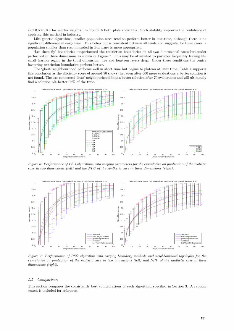
and 0.5 to 0.8 for inertia weights. In Figure 6 both plots show this. Such stability improves the confidence ofapplying this method in industry.

Like genetic algorithms, smaller population sizes tend to perform better in late time, although there is nosignificant difference in early time. This behaviour is consistent between all trials and suggests, for these cases, apopulation smaller than recommended in literature is more appropriate.

‘Let them fly’ boundaries outperformed the restriction boundaries on all two dimensional cases but underperformed in three dimensions as shown in Figure 7. This may be attributed to particles frequently leaving thesmall feasible region in the third dimension: five and fourteen layers deep. Under these conditions the centrefavouring restriction boundaries perform better.

The ‘gbest’ neighbourhood performs well in short time but begins to plateau at later time. Table 4 supportsthis conclusion as the efficiency score of around 50 shows that even after 600 more evaluations a better solution isnot found. The less connected ‘lbest’ neighbourhood finds a better solution after 70 evaluations and will ultimatelyfind a solution 6% better 95% of the time.

0 10 20 30 40 50 60 70 80 90 1000.5

0.55

0.6

0.65

0.7

0.75

0.8

0.85

0.9

0.95

1Selected Particle Swarm Optimisation Trials for COP from the Real Reservoir in 2D

Unique Function Evaluations

Mea

n E

ffect

iven

ess

ltf neumann 3pp (Control)0.5inertia0.9inertia1.1inertia1pb2pb5pb1gb2gb5gb

0 10 20 30 40 50 60 70 80 90 1000.5

0.55

0.6

0.65

0.7

0.75

0.8

0.85

0.9

0.95

1Selected Particle Swarm Optimisation Trials for NPV from the Synthetic Reservoir in 3D

Unique Function Evaluations

Mea

n E

ffect

iven

ess

1pggb2pbgb5pbgb

Figure 6: Performance of PSO algorithms with varying parameters for the cumulative oil production of the realisticcase in two dimensions (left) and the NPC of the synthetic case in three dimensions (right).

0 10 20 30 40 50 60 70 80 90 1000.5

0.55

0.6

0.65

0.7

0.75

0.8

0.85

0.9

0.95

1Selected Particle Swarm Optimisation Trials for COP from the Real Reservoir in 2D

Unique Function Evaluations

Mea

n E

ffect

iven

ess

Standardlbest neighbourhoodgbest neighbourhoodeuclideanLet Them Fly Boundaries

0 10 20 30 40 50 60 70 80 90 1000.5

0.55

0.6

0.65

0.7

0.75

0.8

0.85

0.9

0.95

1Selected Particle Swarm Optimisation Trials for NPV from the Synthetic Reservoir in 3D

Unique Function Evaluations

Mea

n E

ffect

iven

ess

Standardlbest neighbourhoodgbest neighbourhoodeuclideanLet Them Fly Boundaries

Figure 7: Performance of PSO algorithm with varying boundary methods and neighbourhood topologies for thecumulative oil production of the realistic case in two dimensions (left) and NPV of the synthetic case in threedimensions (right).

4.5 Comparison

This section compares the consistently best configurations of each algorithm, specified in Section 3. A randomsearch is included for reference.

131

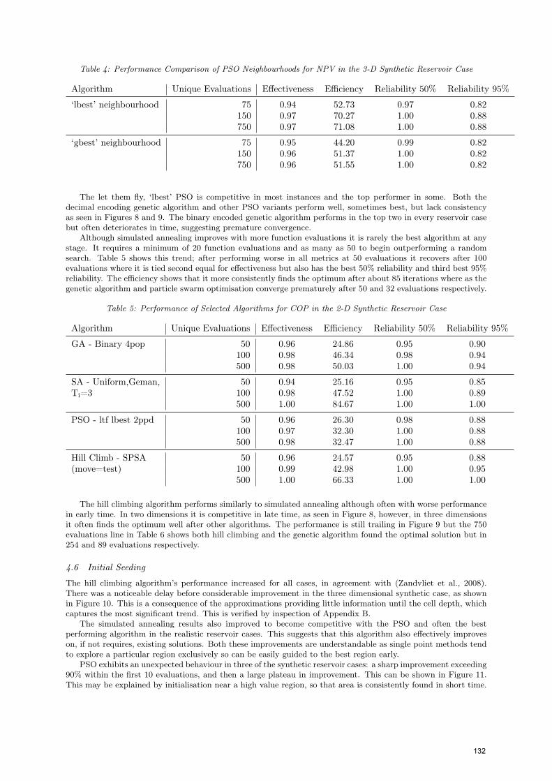
Table 4: Performance Comparison of PSO Neighbourhoods for NPV in the 3-D Synthetic Reservoir Case

Algorithm Unique Evaluations Effectiveness Efficiency Reliability 50% Reliability 95%

‘lbest’ neighbourhood 75 0.94 52.73 0.97 0.82150 0.97 70.27 1.00 0.88750 0.97 71.08 1.00 0.88

‘gbest’ neighbourhood 75 0.95 44.20 0.99 0.82150 0.96 51.37 1.00 0.82750 0.96 51.55 1.00 0.82

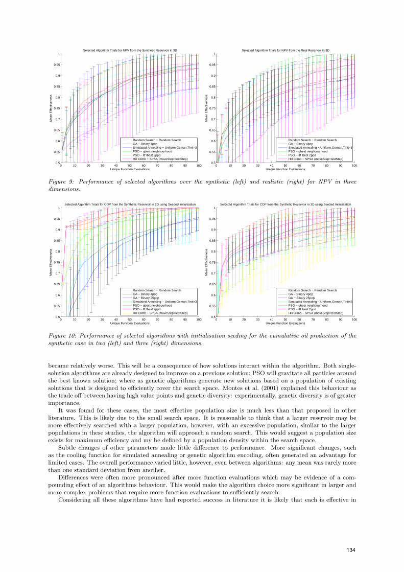
The let them fly, ‘lbest’ PSO is competitive in most instances and the top performer in some. Both thedecimal encoding genetic algorithm and other PSO variants perform well, sometimes best, but lack consistencyas seen in Figures 8 and 9. The binary encoded genetic algorithm performs in the top two in every reservoir casebut often deteriorates in time, suggesting premature convergence.

Although simulated annealing improves with more function evaluations it is rarely the best algorithm at anystage. It requires a minimum of 20 function evaluations and as many as 50 to begin outperforming a randomsearch. Table 5 shows this trend; after performing worse in all metrics at 50 evaluations it recovers after 100evaluations where it is tied second equal for effectiveness but also has the best 50% reliability and third best 95%reliability. The efficiency shows that it more consistently finds the optimum after about 85 iterations where as thegenetic algorithm and particle swarm optimisation converge prematurely after 50 and 32 evaluations respectively.

Table 5: Performance of Selected Algorithms for COP in the 2-D Synthetic Reservoir Case

Algorithm Unique Evaluations Effectiveness Efficiency Reliability 50% Reliability 95%

GA - Binary 4pop 50 0.96 24.86 0.95 0.90100 0.98 46.34 0.98 0.94500 0.98 50.03 1.00 0.94

SA - Uniform,Geman, 50 0.94 25.16 0.95 0.85Ti=3 100 0.98 47.52 1.00 0.89

500 1.00 84.67 1.00 1.00

PSO - ltf lbest 2ppd 50 0.96 26.30 0.98 0.88100 0.97 32.30 1.00 0.88500 0.98 32.47 1.00 0.88

Hill Climb - SPSA 50 0.96 24.57 0.95 0.88(move=test) 100 0.99 42.98 1.00 0.95

500 1.00 66.33 1.00 1.00

The hill climbing algorithm performs similarly to simulated annealing although often with worse performancein early time. In two dimensions it is competitive in late time, as seen in Figure 8, however, in three dimensionsit often finds the optimum well after other algorithms. The performance is still trailing in Figure 9 but the 750evaluations line in Table 6 shows both hill climbing and the genetic algorithm found the optimal solution but in254 and 89 evaluations respectively.

4.6 Initial Seeding

The hill climbing algorithm’s performance increased for all cases, in agreement with (Zandvliet et al., 2008).There was a noticeable delay before considerable improvement in the three dimensional synthetic case, as shownin Figure 10. This is a consequence of the approximations providing little information until the cell depth, whichcaptures the most significant trend. This is verified by inspection of Appendix B.

The simulated annealing results also improved to become competitive with the PSO and often the bestperforming algorithm in the realistic reservoir cases. This suggests that this algorithm also effectively improveson, if not requires, existing solutions. Both these improvements are understandable as single point methods tendto explore a particular region exclusively so can be easily guided to the best region early.

PSO exhibits an unexpected behaviour in three of the synthetic reservoir cases: a sharp improvement exceeding90% within the first 10 evaluations, and then a large plateau in improvement. This can be shown in Figure 11.This may be explained by initialisation near a high value region, so that area is consistently found in short time.

132

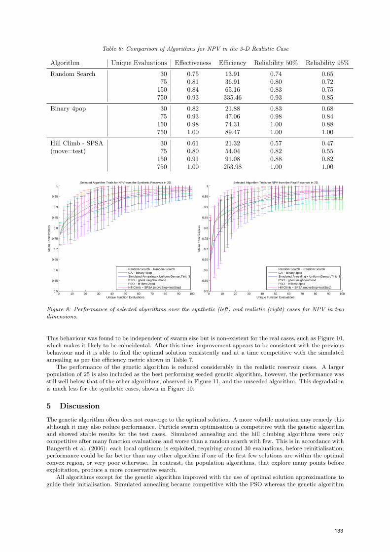
Table 6: Comparison of Algorithms for NPV in the 3-D Realistic Case

Algorithm Unique Evaluations Effectiveness Efficiency Reliability 50% Reliability 95%

Random Search 30 0.75 13.91 0.74 0.6575 0.81 36.91 0.80 0.72

150 0.84 65.16 0.83 0.75750 0.93 335.46 0.93 0.85

Binary 4pop 30 0.82 21.88 0.83 0.6875 0.93 47.06 0.98 0.84

150 0.98 74.31 1.00 0.88750 1.00 89.47 1.00 1.00

Hill Climb - SPSA 30 0.61 21.32 0.57 0.47(move=test) 75 0.80 54.04 0.82 0.55

150 0.91 91.08 0.88 0.82750 1.00 253.98 1.00 1.00

0 10 20 30 40 50 60 70 80 90 1000.5

0.55

0.6

0.65

0.7

0.75

0.8

0.85

0.9

0.95

1Selected Algorithm Trials for NPV from the Synthetic Reservoir in 2D

Unique Function Evaluations

Mea

n E

ffect

iven

ess

Random Search − Random SearchGA − Binary 4popSimulated Annealing − Uniform,Geman,Tinit=3PSO − gbest neighbourhoodPSO − ltf lbest 2ppdHill Climb − SPSA (moveStep=testStep)

0 10 20 30 40 50 60 70 80 90 1000.5

0.55

0.6

0.65

0.7

0.75

0.8

0.85

0.9

0.95

1Selected Algorithm Trials for NPV from the Real Reservoir in 2D

Unique Function Evaluations

Mea

n E

ffect

iven

ess

Random Search − Random SearchGA − Binary 4popSimulated Annealing − Uniform,Geman,Tinit=3PSO − gbest neighbourhoodPSO − ltf lbest 2ppdHill Climb − SPSA (moveStep=testStep)

Figure 8: Performance of selected algorithms over the synthetic (left) and realistic (right) cases for NPV in twodimensions.

This behaviour was found to be independent of swarm size but is non-existent for the real cases, such as Figure 10,which makes it likely to be coincidental. After this time, improvement appears to be consistent with the previousbehaviour and it is able to find the optimal solution consistently and at a time competitive with the simulatedannealing as per the efficiency metric shown in Table 7.

The performance of the genetic algorithm is reduced considerably in the realistic reservoir cases. A largerpopulation of 25 is also included as the best performing seeded genetic algorithm, however, the performance wasstill well below that of the other algorithms, observed in Figure 11, and the unseeded algorithm. This degradationis much less for the synthetic cases, shown in Figure 10.

5 Discussion

The genetic algorithm often does not converge to the optimal solution. A more volatile mutation may remedy thisalthough it may also reduce performance. Particle swarm optimisation is competitive with the genetic algorithmand showed stable results for the test cases. Simulated annealing and the hill climbing algorithms were onlycompetitive after many function evaluations and worse than a random search with few. This is in accordance withBangerth et al. (2006): each local optimum is exploited, requiring around 30 evaluations, before reinitialisation;performance could be far better than any other algorithm if one of the first few solutions are within the optimalconvex region, or very poor otherwise. In contrast, the population algorithms, that explore many points beforeexploitation, produce a more conservative search.

All algorithms except for the genetic algorithm improved with the use of optimal solution approximations toguide their initialisation. Simulated annealing became competitive with the PSO whereas the genetic algorithm

133

0 10 20 30 40 50 60 70 80 90 1000.5

0.55

0.6

0.65

0.7

0.75

0.8

0.85

0.9

0.95

1Selected Algorithm Trials for NPV from the Synthetic Reservoir in 3D

Unique Function Evaluations

Mea

n E

ffect

iven

ess

Random Search − Random SearchGA − Binary 4popSimulated Annealing − Uniform,Geman,Tinit=3PSO − gbest neighbourhoodPSO − ltf lbest 2ppdHill Climb − SPSA (moveStep=testStep)

0 10 20 30 40 50 60 70 80 90 1000.5

0.55

0.6

0.65

0.7

0.75

0.8

0.85

0.9

0.95

1Selected Algorithm Trials for NPV from the Real Reservoir in 3D

Unique Function Evaluations

Mea

n E

ffect

iven

ess

Random Search − Random SearchGA − Binary 4popSimulated Annealing − Uniform,Geman,Tinit=3PSO − gbest neighbourhoodPSO − ltf lbest 2ppdHill Climb − SPSA (moveStep=testStep)

Figure 9: Performance of selected algorithms over the synthetic (left) and realistic (right) for NPV in threedimensions.

0 10 20 30 40 50 60 70 80 90 1000.5

0.55

0.6

0.65

0.7

0.75

0.8

0.85

0.9

0.95

1Selected Algorithm Trials for COP from the Synthetic Reservoir in 2D using Seeded Initialisation

Unique Function Evaluations

Mea

n E

ffect

iven

ess

Random Search − Random SearchGA − Binary 4popGA − Binary 25popSimulated Annealing − Uniform,Geman,Tinit=3PSO − gbest neighbourhoodPSO − ltf lbest 2ppdHill Climb − SPSA (moveStep=testStep)

0 10 20 30 40 50 60 70 80 90 1000.5

0.55

0.6

0.65

0.7

0.75

0.8

0.85

0.9

0.95

1Selected Algorithm Trials for COP from the Synthetic Reservoir in 3D using Seeded Initialisation

Unique Function Evaluations

Mea

n E

ffect

iven

ess

Random Search − Random SearchGA − Binary 4popGA − Binary 25popSimulated Annealing − Uniform,Geman,Tinit=3PSO − gbest neighbourhoodPSO − ltf lbest 2ppdHill Climb − SPSA (moveStep=testStep)

Figure 10: Performance of selected algorithms with initialisation seeding for the cumulative oil production of thesynthetic case in two (left) and three (right) dimensions.

became relatively worse. This will be a consequence of how solutions interact within the algorithm. Both single-solution algorithms are already designed to improve on a previous solution; PSO will gravitate all particles aroundthe best known solution; where as genetic algorithms generate new solutions based on a population of existingsolutions that is designed to efficiently cover the search space. Montes et al. (2001) explained this behaviour asthe trade off between having high value points and genetic diversity: experimentally, genetic diversity is of greaterimportance.

It was found for these cases, the most effective population size is much less than that proposed in otherliterature. This is likely due to the small search space. It is reasonable to think that a larger reservoir may bemore effectively searched with a larger population, however, with an excessive population, similar to the largerpopulations in these studies, the algorithm will approach a random search. This would suggest a population sizeexists for maximum efficiency and my be defined by a population density within the search space.

Subtle changes of other parameters made little difference to performance. More significant changes, suchas the cooling function for simulated annealing or genetic algorithm encoding, often generated an advantage forlimited cases. The overall performance varied little, however, even between algorithms: any mean was rarely morethan one standard deviation from another.

Differences were often more pronounced after more function evaluations which may be evidence of a com-pounding effect of an algorithms behaviour. This would make the algorithm choice more significant in larger andmore complex problems that require more function evaluations to sufficiently search.

Considering all these algorithms have had reported success in literature it is likely that each is effective in

134

0 10 20 30 40 50 60 70 80 90 1000.5

0.55

0.6

0.65

0.7

0.75

0.8

0.85

0.9

0.95

1Selected Algorithm Trials for NPV from the Real Reservoir in 2D using Seeded Initialisation

Unique Function Evaluations

Mea

n E

ffect

iven

ess

Random Search − Random SearchGA − Binary 4popGA − Binary 25popSimulated Annealing − Uniform,Geman,Tinit=3PSO − gbest neighbourhoodPSO − ltf lbest 2ppdHill Climb − SPSA (moveStep=testStep)

0 10 20 30 40 50 60 70 80 90 1000.5

0.55

0.6

0.65

0.7

0.75

0.8

0.85

0.9

0.95

1Selected Algorithm Trials for NPV from the Real Reservoir in 3D using Seeded Initialisation

Unique Function Evaluations

Mea

n E

ffect

iven

ess

Random Search − Random SearchGA − Binary 4popGA − Binary 25popSimulated Annealing − Uniform,Geman,Tinit=3PSO − gbest neighbourhoodPSO − ltf lbest 2ppdHill Climb − SPSA (moveStep=testStep)

Figure 11: Performance of selected algorithms with initialisation seeding for the NPV of the real case in two (left)and three (right) dimensions.

Table 7: Performance of Algorithms with Initialisation Seeding for COP in the 2-D Realistic Reservoir Case

Algorithm Evaluations Effectiveness Efficiency Reliability 50% Reliability 95%

GA - Binary 4pop 500 0.98 65.92 1.00 0.91SA - Uniform,Geman,Ti=3 500 1.00 34.41 1.00 1.00PSO - ltf lbest 2ppd 500 1.00 35.06 1.00 1.00Hill Climb - Orthogonal 500 1.00 57.42 1.00 1.00Hill Climb - SPSAvar 500 1.00 57.66 1.00 1.00

certain circumstances but results may not be transferable. Hence, extrapolation from these or other studies shouldbe done cautiously and ideally verified experimentally. This would also suggest a method of characterising reser-voirs and measuring performance against these characterisations be hugely beneficial in both selecting appropriatealgorithms and understanding algorithm behaviour for the design of new algorithms.

6 Conclusion

It is clear from literature that some method of benchmarking is required to compare the many algorithm variationsused for reservoir optimisation. This is attempted here by testing a selection of the most common algorithmsagainst two, simple, single well-placement reservoir problems.

The genetic algorithm, as the most popular method in literature, and particle swarm optimisation bothperformed well in most cases tested. Both simulated annealing and the hill climbing algorithms perform poorly,often worse than a random search until after as many as 100 evaluations. All algorithms except for the geneticalgorithm improved with the incorporation of a priori knowledge, particularly simulated annealing which becamecompetitive with the PSO.

Based on these results, particle swarm optimisation is recommended as it is the most durable with andwithout guided initialisation. Simulated annealing could also be considered, although guided initialisation isalmost essential otherwise performance is worse than a random search for a considerable number of evaluations.Seeding, however, has variable results with population-based searches and should not be used in conjunction withgenetic algorithms.

The conclusions drawn from these experiments are limited due to computational resources restricting thereservoir sample size to two and the problem formulation to the location of only a single well. Computationalrestrictions are common and is likely the cause of the systemic lack of algorithm benchmarking for reservoir optim-isation. Still, some valuable insight can be gained from these experiments that could guide further investigation.

This study should be extended to contain more test cases, preferably covering a range of complexities andtypical variations in formation, properties and configuration; and a more comprehensive selection of algorithmsincluding interpolation methods, adjoint methods and hybrid methods. This could benchmark algorithms to vetnew developments to ensure a high quality of those implemented. It also has the potential to provide more insightinto algorithm behaviour and guide the design of such algorithms based on their relative improvement rates at

135

different phases.

References

Aanonsen, S., Eide, A., Holden, L., and Aasen, J. (1995). Optimizing reservoir performance under uncertaintywith application to well location. In SPE Annual Technical Conference and Exhibition.

Badru, O. and Kabir, C. (2003). Well placement optimization in field development. In SPE Annual TechnicalConference and Exhibition.

Bangerth, W., Klie, H., Wheeler, M., Stoffa, P., and Sen, M. (2006). On optimization algorithms for the reservoiroil well placement problem. Springer Science.

Beckner, B. and Song, X. (1995). Field development planning using simulated annealing-optimal economic wellscheduling and placement. In SPE Annual Technical Conference and Exhibition.

Bittencourt, A. and Horne, R. (1997). Reservoir development and design optimization. Paper SPE, 38895:5–8.

Bratton, D. and Kennedy, J. (2007). Defining a standard for particle swarm optimization. In Swarm IntelligenceSymposium, 2007. SIS 2007. IEEE, pages 120–127. IEEE.

Ciaurri, D., Mukerji, T., and Durlofsky, L. (2011). Derivative-free optimization for oil field operations. In Yang,X.-S. and Koziel, S., editors, Computational Optimization and Applications in Engineering and Industry, volume359 of Studies in Computational Intelligence, pages 19–55. Springer Berlin / Heidelberg. 10.1007/978-3-642-20986-4_2.

Clerc, M. (2011). From Theory to Practice in Particle Swarm Optimization in the Handbook of Swarm Intelligence,pages 3–36. Springer.

Ding, D. (2008). Optimization of well placement using evolutionary algorithms. In SPE Europec/EAGE Annualconference and exhibition.

ECLIPSE (2009). 2009.1. Schlumberger, Houston, Texas.

Guyaguler, B., Home, R., Rogers, L., and Rosenzweig, J. (2002). Optimization of well placement in a gulf ofmexico waterflooding project. SPE Reservoir Evaluation & Engineering, 5(3):229–236.

Houck, C., J.Joines, and M.Kay (1996). A genetic algorithm for function optimization: A MATLAB implement-ation. ACM Transactions on Mathmatical Software.

Ingber, L. (1996). Adaptive simulated annealing (asa): Lessons learned. In Control and Cybernetics. Citeseer.

Kennedy, J. (2002). Population structure and particle swarm performance. In In: Proceedings of the Congress onEvolutionary Computation (CEC 2002, pages 1671–1676. IEEE Press.

Kennedy, J. and Eberhart, R. C. (1995). Particle swarm optimization. In Proc. IEEE International Conferenceon Neural Networks (Perth, Australia), pages IV: 1942–1948, IEEE Service Center, Piscataway, NJ.

Kennedy, J. and Mendes, R. (2006). Neighborhood topologies in fully informed and best-of-neighborhood particleswarms. Systems, Man, and Cybernetics, Part C: Applications and Reviews, IEEE Transactions on, 36(4):515–519.

Lo, K., Starley, G., and Holden, C. (1995). Application of linear programming to reservoir development evalu-ations. SPE Reservoir Engineering, 10(1):52–58.

MATLAB (2010). version 7.10 (R2010a). The MathWorks Inc., Natick, Massachusetts.

Montes, G., Bartolome, P., and Udias, A. (2001). The use of genetic algorithms in well placement optimization.In SPE Latin American and Caribbean Petroleum Engineering Conference.

Morales, A., Nasrabadi, H., and Zhu, D. (2011). A new modified genetic algorithm for well placement optimizationunder geological uncertainties. In SPE EUROPEC/EAGE Annual Conference and Exhibition.

Nakajima, L. and Schiozer, D. (2003). Horizontal well placement optimization using quality map definition. InCanadian International Petroleum Conference.

136

Onwunalu, J. and Durlofsky, L. (2009a). Development and application of a new well pattern optimization al-gorithm for optimizing large scale field development. In SPE Annual Technical Conference and Exhibition.

Onwunalu, J. E. and Durlofsky, L. J. (2009b). Application of a particle swarm optimization algorithm fordetermining optimum well location and type. Springer Science.

Pan, Y. and Horne, R. (1998). Improved methods for multivariate optimization of field development schedulingand well placement design. In SPE Annual Technical Conference and Exhibition.

Poli, R., Kennedy, J., and Blackwell, T. (2007). Particle swarm optimization an overview. Springer Science.

Salamon, P., Frost, R., and Sibani, P. (2002). Facts, Conjectures, and Improvements for Simulated Annealing.Society for Industrial and Applied Mathematics, Philadelphia, PA, USA.

Sarma, P. and Chen, W. H. (2008). Efficient well placement optimization with gradient-based algorithms andadjoint models. SPE International.

Shi, Y. and Eberhart, R. (1998). A modified particle swarm optimizer. In Proc. of the 1998 IEEE Congress onEvolutionary Computation, Anchorage, AK.

Spall, J. (1992). Multivariate stochastic approximation using a simultaneous perturbation gradient approximation.Automatic Control, IEEE Transactions on, 37(3):332–341.

Tupac, Y., Almeida, L., Almeida, L., and Vellasco, M. (2007). Evolutionary optimization of oil field development.In Digital Energy Conference and Exhibition, Houston, Texas, U.S.A.

Wang, C., Li, G., and Reynolds, A. (2007). Optimal well placement for production optimization. In EasternRegional Meeting, Lexington, Kentucky USA.

Zandvliet, M., Handels, M., van Essen, G., Brouwer, R., and Jansen, J. (2008). Adjoint-based well-placementoptimization under production constraints. SPE Journal, 13(4):392–399.

Zangl, G., Graf, T., and Al-Kinani, A. (2006). Proxy Modeling in Production Optimization. In SPE Euro-pec/EAGE Annual Conference and Exhibition, Vienna, Austria.

137

A Simulated Functions

0

5

10

15

20

0

5

10

15

20

25

2

2.2

2.4

2.6

2.8

3

x 107

Cell layer 1

05

1015

20

0

5

10

15

20

25

5

5.5

6

6.5

7

x 108

Cell layer 1

0

5

10

15

20

0

5

10

15

20

25

2

2.2

2.4

2.6

2.8

3

x 107

Cell layer 4

05

1015

20

0

5

10

15

20

25

5

5.5

6

6.5

7

x 108

Cell layer 4

0

5

10

15

20

0

5

10

15

20

25

2

2.2

2.4

2.6

2.8

3

x 107

Cell layer 7

05

1015

20

0

5

10

15

20

25

5

5.5

6

6.5

7

x 108

Cell layer 7

0

5

10

15

20

0

5

10

15

20

25

2

2.2

2.4

2.6

2.8

3

x 107

Cell layer 10

05

1015

20

0

5

10

15

20

25

5

5.5

6

6.5

7

x 108

Cell layer 10

0

5

10

15

20

0

5

10

15

20

25

2

2.2

2.4

2.6

2.8

3

x 107

Cell layer 13

05

1015

20

0

5

10

15

20

25

5

5.5

6

6.5

7

x 108

Cell layer 13

Figure 12: COP in barrels (left) and NPV in dollars (right) over the new well locations in the synthetic reservoirfor five selected lower perforation limits.

138

0

1020

30

40

50

0

10

20

30

40

50

2

3

4

5

6

7

x 106

Cell layer 1

010

2030

4050

0

10

20

30

40

50

1

2

3

4

5

6

7

x 107

Cell layer 1

0

1020

30

40

50

0

10

20

30

40

50

2

3

4

5

6

7

x 106

Cell layer 2

010

2030

4050

0

10

20

30

40

50

1

2

3

4

5

6

7

x 107

Cell layer 2

0

1020

30

40

50

0

10

20

30

40

50

2

3

4

5

6

7

x 106

Cell layer 3

010

2030

4050

0

10

20

30

40

50

1

2

3

4

5

6

7

x 107

Cell layer 3

0

1020

30

40

50

0

10

20

30

40

50

2

3

4

5

6

7

x 106

Cell layer 4

010

2030

4050

0

10

20

30

40

50

1

2

3

4

5

6

7

x 107

Cell layer 4

0

1020

30

40

50

0

10

20

30

40

50

2

3

4

5

6

7

x 106

Cell layer 5

010

2030

4050

0

10

20

30

40

50

1

2

3

4

5

6

7

x 107

Cell layer 5

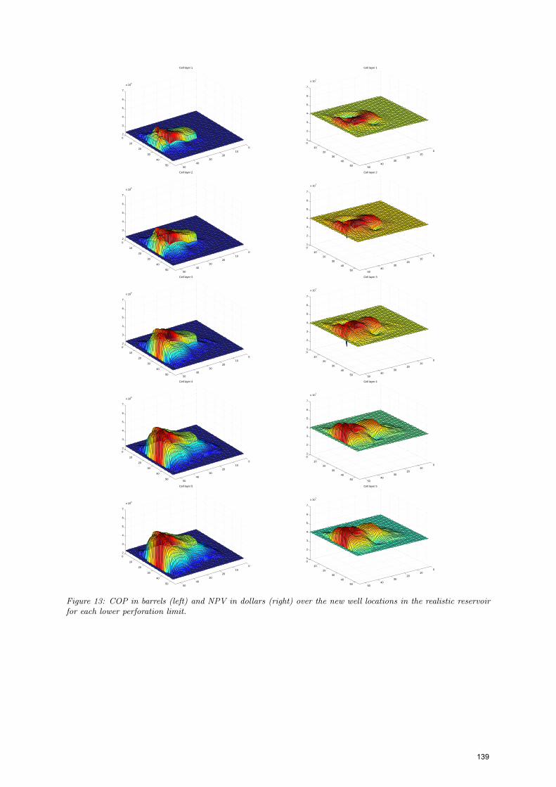
Figure 13: COP in barrels (left) and NPV in dollars (right) over the new well locations in the realistic reservoirfor each lower perforation limit.

139

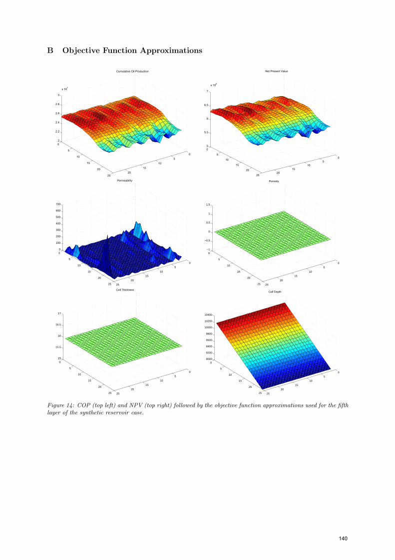
B Objective Function Approximations

0

5

10

15

20

0

5

10

15

20

25

2

2.2

2.4

2.6

2.8

3

x 107

Cumulative Oil Production

0

5

10

15

20

0

5

10

15

20

25

5

5.5

6

6.5

7

x 108

Net Present Value

0

5

10

15

20

25

0

5

10

15

20

25

0

100

200

300

400

500

600

700

Permeability

0

5

10

15

20

25

0

5

10

15

20

25

−1

−0.5

0

0.5

1

1.5

Porosity

0

5

10

15

20

25

0

5

10

15

20

25

15

15.5

16

16.5

17

Cell Thickness

0

5

10

15

20

25

0

5

10

15

20

25

9000

9200

9400

9600

9800

10000

10200

10400

Cell Depth

Figure 14: COP (top left) and NPV (top right) followed by the objective function approximations used for the fifthlayer of the synthetic reservoir case.

140

0

10

20

30

40

50

0

10

20

30

40

50

2

3

4

5

6

7

x 106

Cumulative Oil Production

0

10

20

30

40

50

0

10

20

30

40

50

1

2

3

4

5

6

7

x 107

Net Present Value

010

2030

4050

60

0

10

20

30

40

50

60

0

0.5

1

1.5

2

2.5

x 106

Well Pressure Index

010

2030

4050

60

0

10

20

30

40

50

60

20

30

40

50

60

70

Permeability

010

2030

4050

60

0

10

20

30

40

50

60

−1

−0.5

0

0.5

1

1.5

Porosity

010

2030

4050

60

0

10

20

30

40

50

60

0

2

4

6

8

10

Cell Thickness

010

2030

4050

60

0

10

20

30

40

50

60

−10000

−8000

−6000

−4000

−2000

0

Cell Depth

010

2030

4050

60

0

10

20

30

40

50

60

0

0.2

0.4

0.6

0.8

1

Net to Gross

Figure 15: COP (top left) and NPV (top right) followed by the objective function approximations used for the fifthlayer of the realistic reservoir case.

141