A Comparison of Blocking & Non-Blocking Synchronization
100
A Comparison of Blocking & Non-Blocking Synchronization Kevin Chirls Advisor: Prof. Tim Huang Senior Thesis in Computer Science Middlebury College May 2007
Transcript of A Comparison of Blocking & Non-Blocking Synchronization
A Comparison of Blocking & Non-Blocking
Synchronization
Kevin Chirls
Advisor: Prof. Tim Huang
Senior Thesis in Computer Science Middlebury College
May 2007

ii
Abstract
Synchronization is the problem of coordinating multiple events across time within
a single system, such that the parallel events occur successfully without collisions.
Computers use many different forms of synchronization for controlling hardware access,
shared memory, shared files, process execution, as well as the handling of numerous
other resources. It is especially important for data structures in a parallel processing
environment. The status quo and most commonly used implementation of
synchronization is blocking synchronization, which utilizes locks to prevent conflicts
between competing processes. This thesis explores and compares the alternative of non-
blocking synchronization, which does not employ locks, but instead complex algorithms
using hardware-based primitive atomic operations.

iii
Acknowledgements I, of course, must first thank my advisor, Prof. Tim Huang, for aiding me on this
path into realms unknown. Second, I would like to thank Prof. Bob Martin for helping
me find a “working” multiprocessor machine. I would like to thank Prof. Matt Dickerson
for leading the thesis seminar and reminding us, every so often, that there is always more
work to be done. I would also like to thank the entire computer science department for
providing the knowledge and opportunity to delve into the world that is computer
science. At times it can seem daunting, but in the end, it is one heck of a rollercoaster
ride! Lastly, I would like to especially thank Anna Blasiak and Jeff Wehrwein. At a
small liberal arts college where students know little about computer science, it is
comforting having peers to relate with.
To others who have contributed bits and pieces along the way, thank you.

iv
Contents Abstract . . . . . . . . . . . . . . . . . . . . . . . . . . . . . . . . . . . . . . . . . . . . . . . . . . . ii Acknowledgements . . . . . . . . . . . . . . . . . . . . . . . . . . . . . . . . . . . . . . . . . . iii 1 Sychronization 1 1.1 Process States . . . . . . . . . . . . . . . . . . . . . . . . . . . . . . . . . . . . . . . . 2 1.2 The Producer/Consumer Problem . . . . . . . . . . . . . . . . . . . . . . . . . 5 1.3 The Critical Section/Mutual Exclusion Problem . . . . . . . . . . . . . 7
2 Atomic Operations 11 2.1 Atomicity in Peterson’s Algorithm . . . . . . . . . . . . . . . . . . . . . . . . 11 2.2 Atomicity in Hardware . . . . . . . . . . . . . . . . . . . . . . . . . . . . . . . . . 14 2.3 Common Operations . . . . . . . . . . . . . . . . . . . . . . . . . . . . . . . . . . . 15 2.4 Using Atomic Operations . . . . . . . . . . . . . . . . . . . . . . . . . . . . . . . 18 3 Blocking Synchronization 23
3.1 Why Blocking? . . . . . . . . . . . . . . . . . . . . . . . . . . . . . . . . . . . . . . . 23 3.2 Semaphores . . . . . . . . . . . . . . . . . . . . . . . . . . . . . . . . . . . . . . . . . . 25 3.3 A Blocking Mutex . . . . . . . . . . . . . . . . . . . . . . . . . . . . . . . . . . . . . 27 3.4 Blocking Pros and Cons . . . . . . . . . . . . . . . . . . . . . . . . . . . . . . . . 30 4 Non-Blocking Synchronization 33 4.1 The Terms . . . . . . . . . . . . . . . . . . . . . . . . . . . . . . . . . . . . . . . . . . . 33 4.2 The Blurring of the Critical Section . . . . . . . . . . . . . . . . . . . . . . . 35 4.3 The ABA Problem . . . . . . . . . . . . . . . . . . . . . . . . . . . . . . . . . . . . . 38 4.4 Livelock . . . . . . . . . . . . . . . . . . . . . . . . . . . . . . . . . . . . . . . . . . . . . 42 5 The Queue 45 5.1 Queue’s Properties . . . . . . . . . . . . . . . . . . . . . . . . . . . . . . . . . . . . . 45 5.2 A Blocking Queue . . . . . . . . . . . . . . . . . . . . . . . . . . . . . . . . . . . . . 47 5.3 A Lock-Free Queue . . . . . . . . . . . . . . . . . . . . . . . . . . . . . . . . . . . . 50 5.4 Linearizable and Non-Blocking . . . . . . . . . . . . . . . . . . . . . . . . . . . 54 6 Blocking vs. Non-Blocking 57 6.1 Non-Blocking Queue . . . . . . . . . . . . . . . . . . . . . . . . . . . . . . . . . . . 57 6.2 Blocking Queue . . . . . . . . . . . . . . . . . . . . . . . . . . . . . . . . . . . . . . . 61 6.3 Barrier and Statistics . . . . . . . . . . . . . . . . . . . . . . . . . . . . . . . . . . . 61 6.4 The Simulation . . . . . . . . . . . . . . . . . . . . . . . . . . . . . . . . . . . . . . . . 63 6.5 Results . . . . . . . . . . . . . . . . . . . . . . . . . . . . . . . . . . . . . . . . . . . . . . 64 7 Conclusion 69 Appendix (source code) . . . . . . . . . . . . . . . . . . . . . . . . . . . . . . . . . . . . . . . . . . . . . 73 Bibliography . . . . . . . . . . . . . . . . . . . . . . . . . . . . . . . . . . . . . . . . . . . . . . . . . . . . . . 99

1
Chapter 1 Synchronization
Modern operating systems support multiplexing1 Central Processing Units (CPUs)
that can handle multiple concurrently running processes. A process, a program in
execution [10, p. 85], can be represented as a single unit that works independently from
other processes on the machine. However, like any independent person, the process
remains an individual that also attempts to work with or alongside other processes. They
can interact by sharing data in a number of ways, including messaging,2 shared files, and
shared logical memory addresses [10, p. 209]. Messaging and file sharing generally
result in simple communication schemes because utilizing access to the underlying
messaging or file system prevents processes from interleaving their instructions.
However, messaging and file communication is slow. Sharing memory is much faster,
but with the power of shared memory comes the risk of interleaving instructions in ways
that can result in corrupt or inconsistent data.
1 Multiplexing can refer to many different individual situations, but generally it defines the concept where multiple signals are combined together to form a complex signal that is passed along a path. The receiving end is then able to divide the complex structure back into its individual parts. Thus, when referring to a multiplexing Central Processing Unit, it indicates that the CPU is able to handle a conglomerate of processes individually through a multiplexing strategy. 2 Process messaging is usually handled by constructing pipes that connect a process’s input and output to another process. The transmission is sent as bytes of data, similar to a networking protocol.

CHAPTER 1. SYNCHRONIZATION
2
To prevent this, modern operating systems and CPUs facilitate synchronization, a
mechanism for handling the issue of data inconsistency in a multiprogramming
environment using shared data. Synchronization can be used to address two different
problems; contention and cooperation [12, p. 2]. The contention problem involves
resolving the issue of multiple processes competing for the same resources. Similar to
the resource allocation problem,3 this issue is generally defined as either the critical
section problem or the mutual exclusion problem. Cooperation, or coordination, is the
way that processes communicate among themselves or the way they work together to
achieve a common goal.4
The following section defines some of the basic states that a process enters in
order to understand why synchronization is required among multiple processes.
1.1 Process States
To better illustrate why synchronization is important with shared memory
addresses by processes, the general states of a process must first be properly defined.
Each process goes through multiple state transitions, which is important since only one
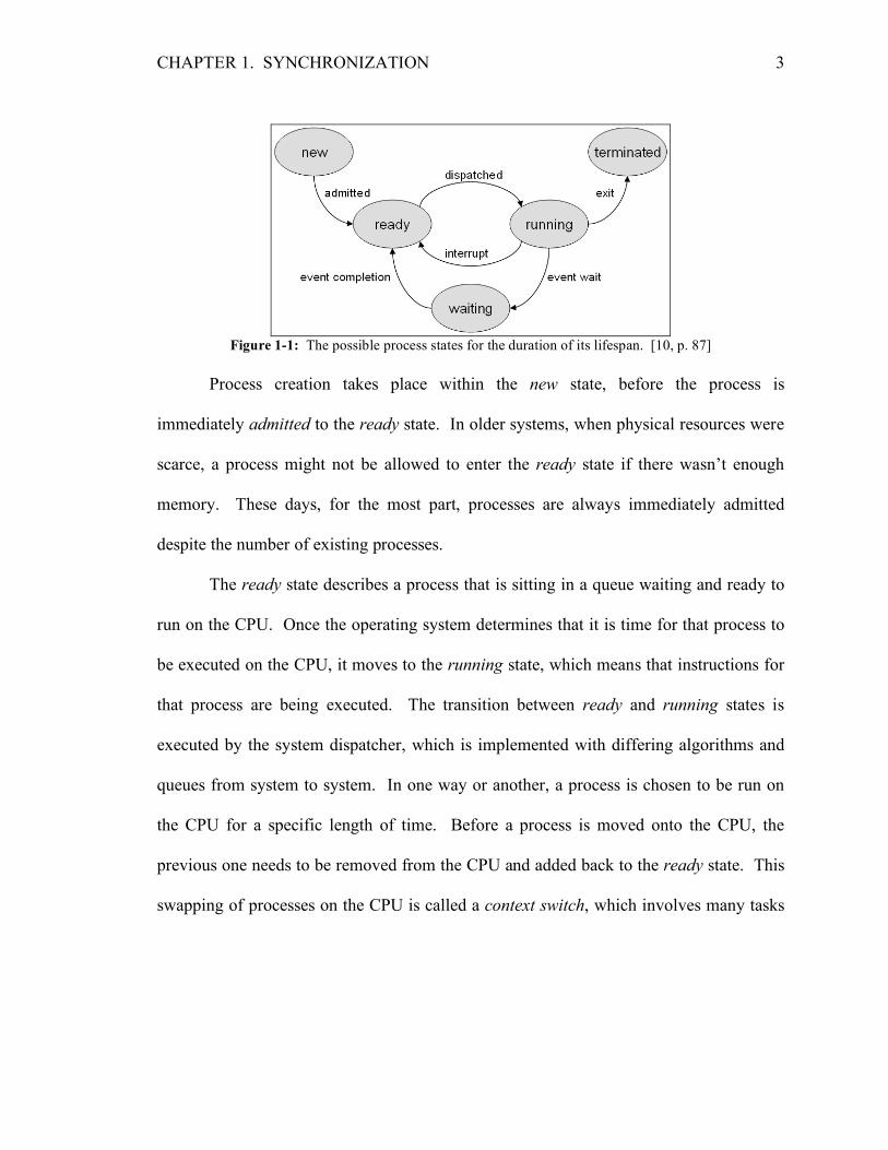
process at a time can be running on a CPU. Figure 1-1 depicts the basic states of a
process.5
3 The resource allocation problem refers to any situation where conflicts can arise from competing entities over a resource or set of resources, such that corrupt data, inconsistent data, or deadlock (see Section 1.2) can occur. 4 Besides processes, there is another layer of parallelism that exists within each process context. The concurrent entities within that layer are called threads. Synchronization applies to either or both processes and threads, depending on the implementation. For simplicity, this paper will mostly refer to an individually running entity as a process, but the paper could easily be applied to threads with little or no changes. 5 There are other possible states in the process state diagram, but for the sake of explaining the mechanisms involved in synchronization, the as-defined diagram is sufficient. The other states can be found in [10, p. 93] where the medium-term scheduler is explained.
CHAPTER 1. SYNCHRONIZATION
3
Figure 1-1: The possible process states for the duration of its lifespan. [10, p. 87]
Process creation takes place within the new state, before the process is
immediately admitted to the ready state. In older systems, when physical resources were
scarce, a process might not be allowed to enter the ready state if there wasn’t enough
memory. These days, for the most part, processes are always immediately admitted
despite the number of existing processes.
The ready state describes a process that is sitting in a queue waiting and ready to
run on the CPU. Once the operating system determines that it is time for that process to
be executed on the CPU, it moves to the running state, which means that instructions for
that process are being executed. The transition between ready and running states is
executed by the system dispatcher, which is implemented with differing algorithms and
queues from system to system. In one way or another, a process is chosen to be run on
the CPU for a specific length of time. Before a process is moved onto the CPU, the
previous one needs to be removed from the CPU and added back to the ready state. This
swapping of processes on the CPU is called a context switch, which involves many tasks

CHAPTER 1. SYNCHRONIZATION
4
including saving the state6 of the previously run process, loading the state of the new
process, and flushing any caches7 if need be.
A process can be removed from the running state for many possible reasons: a
timer interrupt occurs, an I/O call is made, the process exits, or the process blocks itself.
The hardware timer uses interrupts to ensure that processes are not hogging the CPU and
that other processes get a fair share of execution time. So, the timer will generate an
interrupt that will cause a context switch. The removed process will be preempted8 to the
ready state, while some process from the ready state will be dispatched onto the CPU.
Disk I/O requires one or more disk accesses, which are several orders of magnitude
slower than regular memory accesses. Not waiting for such a transaction to finish, the
CPU moves the process off the processor with another context switch. Instead of
returning to the ready state, the process transitions to the waiting state, where it will
block until an I/O interrupt moves the process back to the ready state. The third way that
a process can leave the running state is when it has exited or has been terminated
manually. The last reason for a process to be removed from the running state is when it
blocks itself. It might block itself to wait for another process to finish a certain
transaction either because of contention or cooperation. In either case, the process will
wait in the waiting state for another to wake it.
With the previously defined states and transitions in mind, the requirement for
synchronization can be more understood through the following example problem.
6 The state of a process is kept in a structure called a Process Control Block or PCB. The PCB is what is loaded/saved onto the CPU and back into memory during a context switch. [4, Lecture 3] 7 The Translation Look-aside Buffer (TLB) for example. [4, Lecture 9] 8 Preemption refers to when the operating system manually decides to pop the currently running process off of the CPU.

CHAPTER 1. SYNCHRONIZATION
5
1.2 The Producer/Consumer Problem
The producer/consumer problem illustrates why synchronization is important.
Two processes, the producer and the consumer, share the same logical address space—
the producer produces information that is consumed by the consumer [4, Lecture 8]. This
problem can be implemented using either an unbounded or bounded buffer; Figure 1-2
shows a bounded buffer implementation.
Figure 1-2: Bounded buffer example of the producer/consumer problem in the C programming language.
The producer follows a simple set of rules—as long as the buffer is full, loop and
wait until it is not. If the buffer is not full, add an item. The producer’s job is simply to
keep the buffer full. The consumer, on the other hand, continually tries to remove items
from the buffer. If the buffer is empty, the consumer loops until it is not. Once not
empty, the consumer removes an item. In this basic example, the two processes work
together with only a few commonly shared variables: count, BUFFER_SIZE, and the
buffer.
Although this code seems to indicate that the two will work together in harmony,
there is in fact a problem. The C code hides the details of the compiled code, which does
not look the same. For example, the shared variable count, which keeps track of the
number of items in the buffer, is incremented in the producer process and decremented in
the consumer process. However, the single lines for these operations are not in fact

CHAPTER 1. SYNCHRONIZATION
6
single step operations. Figure 1-3 depicts the possible low-level instructions for a call to
increment a value by one, and then to decrement a value by one.
Figure 1-3: Low-level pseudo-code instructions for incrementing and decrementing a variable count.
Given the definition in Figure 1-3, context switches can occur causing the
producer and consumer to conflict when modifying the shared variable count. To
illustrate the conflict, let count be the value 5. If 5 is read into register1 by the producer
and register2 by the consumer, then the producer will increment the register to 6, while
the consumer will decrement its register to 4. So, the two processes race against each
other to decide the final value of count, which ends up being 4 or 6 when it should have
been 5. This type of situation is referred to as a race condition, where the result of an
operation is determined by which process finishes it first.
This example of two interleaving processes will result in an inconsistent state for
the variable count. It will not be an accurate sum of the number of items in the buffer.
As a result, the inconsistent data will likely lead to a process crash when either the
producer or consumer attempts to access a piece of the data that does not lie within the
memory confines of that data instance. In other words, one of the processes will try to
use an index on the buffer either less than zero or greater than or equal to the buffer size.
If this occurs, the process will likely terminate unless the error is explicitly handled.
CHAPTER 1. SYNCHRONIZATION
7
This code, where unanticipated results can occur, is called the critical section,
which leads to the definition of the critical section problem, also known as the mutual
exclusion problem.
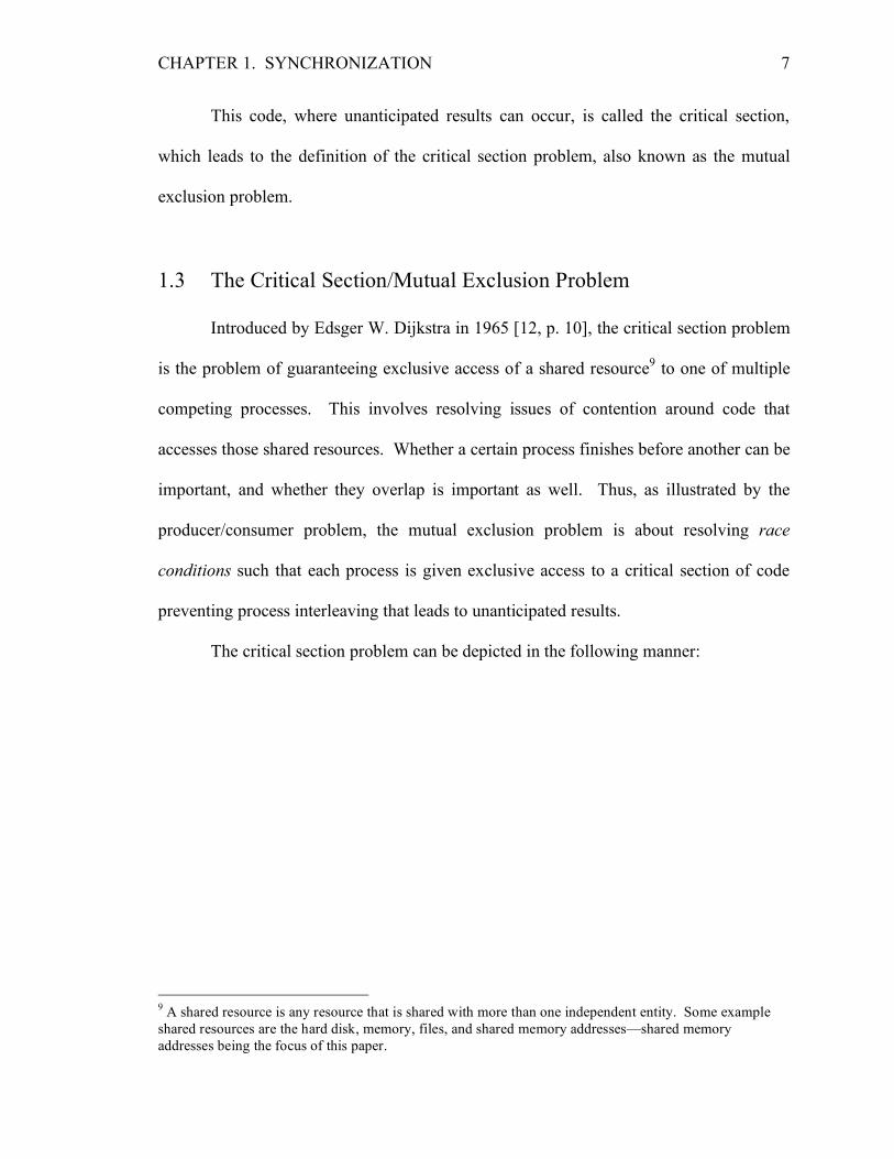
1.3 The Critical Section/Mutual Exclusion Problem
Introduced by Edsger W. Dijkstra in 1965 [12, p. 10], the critical section problem
is the problem of guaranteeing exclusive access of a shared resource9 to one of multiple
competing processes. This involves resolving issues of contention around code that
accesses those shared resources. Whether a certain process finishes before another can be
important, and whether they overlap is important as well. Thus, as illustrated by the
producer/consumer problem, the mutual exclusion problem is about resolving race
conditions such that each process is given exclusive access to a critical section of code
preventing process interleaving that leads to unanticipated results.
The critical section problem can be depicted in the following manner:
9 A shared resource is any resource that is shared with more than one independent entity. Some example shared resources are the hard disk, memory, files, and shared memory addresses—shared memory addresses being the focus of this paper.
CHAPTER 1. SYNCHRONIZATION
8
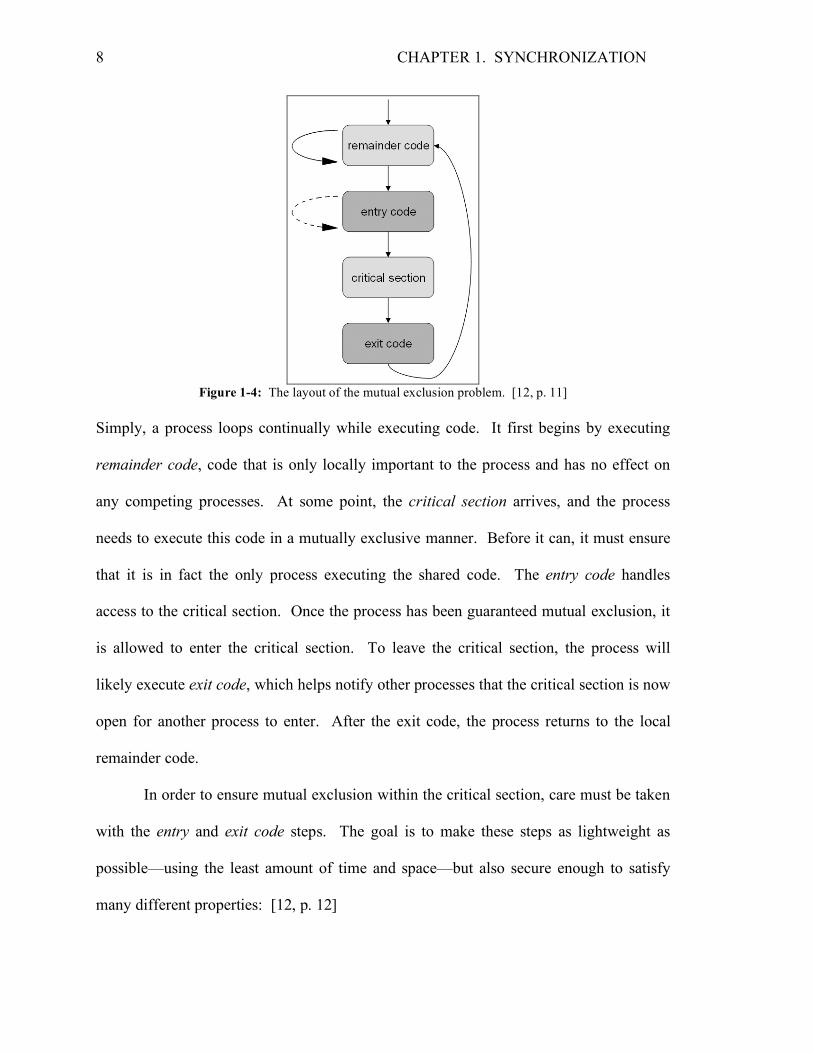
Figure 1-4: The layout of the mutual exclusion problem. [12, p. 11]
Simply, a process loops continually while executing code. It first begins by executing
remainder code, code that is only locally important to the process and has no effect on
any competing processes. At some point, the critical section arrives, and the process
needs to execute this code in a mutually exclusive manner. Before it can, it must ensure
that it is in fact the only process executing the shared code. The entry code handles
access to the critical section. Once the process has been guaranteed mutual exclusion, it
is allowed to enter the critical section. To leave the critical section, the process will
likely execute exit code, which helps notify other processes that the critical section is now
open for another process to enter. After the exit code, the process returns to the local
remainder code.
In order to ensure mutual exclusion within the critical section, care must be taken
with the entry and exit code steps. The goal is to make these steps as lightweight as
possible—using the least amount of time and space—but also secure enough to satisfy
many different properties: [12, p. 12]

CHAPTER 1. SYNCHRONIZATION
9
Mutual Exclusion: No two processes are in their critical section at the same time.
Deadlock-freedom: If a process is trying to enter its critical section, then some process, not necessarily the same one, eventually enters its critical section. The deadlock-freedom property can sometimes be referred to as the global progress property, which guarantees that the system as a whole will always make progress.
Starvation-freedom: If a process is trying to enter its critical section, then this process must eventually enter its critical section. 10
Starvation-freedom is a stronger requirement than deadlock-freedom, since
deadlock-freedom does not guarantee that certain processes will be starved from the
critical section. More precisely, even though deadlock-freedom has explicitly been
handled, a process may sit waiting to enter the critical section forever in the entry code as
other processes beat it out.
Starvation-freedom does not eliminate race conditions entirely, but it does ensure
that a process will eventually enter the critical section. Since race conditions are not
eliminated, a single process might loop back around an arbitrary number of times,
reentering the critical section before a contending process is given access. Stricter and
more precise properties are defined to resolve this issue: [12, p. 49]
Linear-waiting: The term linear-wating is sometimes used in the literature for 1-bounded waiting. Thus, linear-waiting ensures that no process can execute its critical section twice while some other process its kept waiting.
First-in-first-out: The terms first-in-first-out (FIFO), and first-come-first-served (FCFS), are used in the literature for 0-bounded waiting. Thus, first-in-first-out guarantees that: no beginning process can pass an already waiting process (i.e., a process that has already passed through its doorway).
10 A process is starved when it remains in a state indefinitely. Two examples are a process stuck in an infinite loop or deadlock.

CHAPTER 1. SYNCHRONIZATION
10
With the groundwork for synchronization defined, the actual implementation can
be explored. Chapter 2 begins this with the individual primitives built to construct high-
level synchronization solutions.

11
Chapter 2 Atomic Operations
To solve the synchronization problem, basic primitives must be developed that
can handle operations in a mutually exclusive manner. These are atomic, or indivisible,
operations: other concurrent activities do not interfere with their execution [12, p. 147].
This chapter explains why hardware-based atomic operations are necessary to
implemented more sophisticated synchronization. Both common and advanced atomic
operations are defined before illustrating their usage.
2.1 Atomicity in Peterson’s Algorithm
The simplest atomic operations are single read and write operations on atomic
registers that correspond to when a variable is read and when it is assigned. One of the
first synchronization algorithms, designed by Gary L. Peterson in 1981 [12, p. 32], relies
upon this atomicity. However, Peterson’s Algorithm is inherently limited because it only
supports two processes. Figure 2-1 depicts the code implementing this algorithm for
processes P0 and P1.

CHAPTER 2. ATOMIC OPERATIONS
12
Figure 2-1: Peterson’s Algorithm for two contending processes attempting to execute a critical section.1
ready and turn are shared between both processes, but only P0 can write to the 0th
index of ready, and only P1 can write to ready’s 1st index. Both indices are set to false on
startup, and turn’s value is immaterial. For P0’s entry code, when ready[0] is true, it
indicates that P0 is ready to enter the critical section. The same holds for P1 and
ready[1]. turn is used to notify a process of its turn to enter the critical section. The
condition in the while loop, the third line in the entry code, is the test to determine which
process set turn first. Since the second process that reaches this line will set turn to itself,
it allows the earlier process to enter the critical section. This is because both ready
indices will have been set to true. If only P0 had executed this code, then there is no
contention, and it would have immediately been given access to the critical section.
When there is contention, if P0 set turn first, then it will continue on into the critical
section, and P1 will sit in the while statement continually waiting and checking for P0’s
turn to be over with the exit code call to ready[0] = false in P0’s stack. Figure 2-2
diagrams this execution.
1 This slide is based upon the slide provided by [4, Lecture 8] with slight modifications. The array flag was changed to ready to indicate that the process’s relevant array index is used to mark the process as “ready” to enter the critical section. Also, instead of variable-based process IDs i and j, explicit values 1 and 2 are used instead, since in reality Peterson’s Algorithm can only satisfy two processes.

CHAPTER 2. ATOMIC OPERATIONS
13
Figure 2-2: Diagram of Peterson’s Algorithm for Process 0.
This algorithm satisfies both mutual exclusion and starvation-freedom for two
contending processes. Mutual exclusion is satisfied since turn will only allow one
process to continue into the critical section. Starvation-freedom is guaranteed since if P0
finishes and then loops back around and attempts to beat P1 back into the critical section,
it will fail. This is because before P0 enters the critical section it will set turn to itself,
which then invalidates the expression turn == 0 in P1’s code. Therefore, P1 is considered
the first process to cross the barrier.
Again, Peterson’s Solution relies on the fact that the operations on ready and turn
are atomic read and writes. Although this solution works, it is software-based and only
handles two processes. When n processes need to be synchronized, software-based
synchronization algorithms become incredibly complex. For example, if n processes
were attempting to use a similar algorithm to Peterson’s, then an n-length array would be
needed and somehow manipulated to choose which process to proceed. However, there
CHAPTER 2. ATOMIC OPERATIONS
14
is no clear way to decide without creating more complex structures to keep track of
which processes entered the entry code first. However, with more complex structures,
atomic reads and writes are no longer sufficient since the structures can become
inconsistent if they themselves are not properly synchronized. Also, n usually is not
known, so a static array-based implementation can not be used. Thus, software
synchronization is extremely difficult. To implement these more complex algorithms
with simpler means, more advanced hardware-based atomic operations are required.
2.2 Atomicity in Hardware
Software-based implementations using the simple atomic operations read and
write are hard to design and difficult to code. The solution is to implement more
advanced atomic operations at the level of hardware. However, this is not a trivial matter
either.
All computer architectures support atomic operations, but they differ in the actual
atomic operations supported. Atomic read and write are implemented on all
architectures, which means that if a process reads or writes to register r, no other process
can access r at the same time. Taking this one step further, what if a process desires to
increment a register’s value by one? Although this might seem to the programmer like a
single call of r++, it is in fact actually more than one read and write call, as depicted in
Chapter 1 with the producer/consumer problem. In other words, an incrementing
operation is a procedure that would have to be atomic across multiple processor cycles.
As mentioned previously, a context switch can occur at any moment. Depending on the
machine architecture, there is no guaranteed way to determine when and where a context

CHAPTER 2. ATOMIC OPERATIONS
15
switch will occur. To more easily design code with atomicity, some ideas have been put
forth to try and amend the context switch problem.
One solution is to suspend interrupts for the duration of the operation [12, p. 150].
However, this poses multiple issues. For one, it gives control of the interrupt system to
the user program, which might not give it back. Second, most systems depend on
interrupts to continue execution on other processes at the same time, so if interrupts are
disabled for an unknown amount of time, the potential for a process to hog the CPU is
likely. Lastly, disabling interrupts only works on single CPU systems since on a
multiprocessor architecture a disabled interrupt would only affect a single CPU while not
preventing other processors from acting on a shared register.
Current systems implement a more complex scheme that involves a hardware
system linked to one or more processors. It uses special hooks in the multiprocessor
cache coherency strategy, so that the caches for each processor are aware of the current
atomic operation being computed for a specific shared register. This method is usable on
both uni-processor and multiprocessor architectures [12, p. 150].
2.3 Common Operations
Although atomic operations are supported in modern hardware, there are still
limitations on what they can actually accomplish. Up until recently, only atomic
operations with parameters of one shared register and one local register or value were
possible. These operations make up the basic hardware synchronization primitives that
are commonly used today. In [12, p. 148], they are defined as follows:

CHAPTER 2. ATOMIC OPERATIONS
16
Read: takes a register r and returns its value function read(r: register) return: value; return r; end-function Write: takes a shared register r and a value val. The value val is assigned to r. function write(r: register, val: value); r := val; end-function
Test-and-set: takes a shared register r and a value val. The value val is assigned to r, and the old value of r is returned. (In some definitions, val can take only the value 1.)
function test-and-set(r: register, val: value) return: value; temp := r; r := val; return temp; end-function
Swap: takes a shared register r and a local register l, and atomically exchanges their values.
function swap(r: register, l: local-register); temp := r; r := l; l := temp; end-function
Fetch-and-add: takes a register r and a value val. The value of r is incremented by val, and the old value of r is returned. (fetch-and-increment is a special case of this function where val is 1.)
function fetch-and-add(r: register, val: value) return: value; temp := r; r := temp + val; return temp; end-function
Read-modify-write: takes a register r and a function f. The value of f(r) is assigned to r, and the old value of r is returned. Put another way, in one read-modify-write operation a process can atomically read a value of a shared register and then, based on the value read, compute some new value and assign it back to the register. (All the operations mentioned so far are special cases of the read-modify-write operations. In fact, any memory access that consists of reading one shared memory location, performing an arbitrary local computation, and then updating the memory location can be expressed as a read-modify-write operation of the above form.)

CHAPTER 2. ATOMIC OPERATIONS
17
function read-modify-write(r: register, f: function) return: value; temp := r; r := f(r); return temp; end-function Although these operations are enough to implement the primitives and objects necessary
for general synchronization, more complex synchronization schemes, such as non-
blocking synchronization, have been desired. The basic hardware primitives are not
sufficient enough for such algorithms. Recently, more advanced hardware primitives that
can take as parameters two shared registers or one shared register and two local registers
or values have been added to most architectures. The following operations, again defined
in [12, p. 149], are commonly implemented today, usually only one or two per
architecture:
Compare-and-swap: takes a register r and two values: new and old. If the current value of the register r is equal to old, then the value of r is set to new and the value true is returned; otherwise r is left unchanged and the value false is returned.
function compare-and-swap(r: register, old: value, new: value) return: Boolean;
if r == old then r := new; return true;
else return false;
end-if end-function
Sticky-write: takes a register r and a value val. It is assumed that the initial value of r is “undefined” (denoted by � ). If the value of r is � or val, then it is replaced by val, and returns “success”; otherwise r is left unchanged and it returns “fail”. We denote “success” by 1 and “fail” by 0.
Move: takes two shared registers r1 and r2 and atomically copies the value of r2 to r1. The move operation should not be confused with assignment (i.e., write); move copies values between two shared registers, while assignment copies values between shared and private (local) registers.

CHAPTER 2. ATOMIC OPERATIONS
18
function move(r1: register, r2: register); r1 := r2; end-function
Shared-swap: takes two shared registers r1 and r2 and atomically exchanges their values.
function shared-swap(r1: register, r2: register); temp := r1; r1 := r2; r2 := temp; end-function These stronger atomic operations have made more complex algorithms possible.
Nevertheless, some of the basic non-blocking synchronization algorithms still cannot be
solved. Such algorithms require a theoretical operation such as double-compare-and-
swap, or DCAS, which will be discussed further in Chapters 4 and 5. Despite the
advanced operations required for more complex algorithms, the basic operations can still
be used for other solutions, as is exemplified in the next section.
2.4 Using Atomic Operations
An example use of atomic operations is displayed in Figure 2-3 [4, Lecture 8].
Note that both instances use only what are considered basic atomic operations, forms that
are not sufficient for more complicated synchronization algorithms.

CHAPTER 2. ATOMIC OPERATIONS
19
Figure 2-3: Lock-based synchronization approach using a) test-and-set and b) swap.
Figure 2-3a uses test-and-set to implement the locking part of the entry code prior
to entering the critical section. Each process runs the same code and shares a single
register shared_reg. As long as the function returns true,2 it will loop. The call
sched_yield within the loop is a system call that notifies any other processes of similar or
higher priority to execute instead of the calling process. This attempts to keep the
looping process from hogging the CPU when it is not making progress. However, it is
only an attempt, sometimes referred to as a hint to the operating system, and is not
guaranteed to prevent starvation of other processes. A process that makes it passed the
lock retains the lock until it is released by setting the shared register back to false. Once
set back to false, any looping process waiting in the entry code will break out of the loop
on its next atomic test-and-set call, since the call will return false, which does not satisfy
the test within the while statement.
Figure 2-3b is an alternate solution that uses the swap operation instead. Each
process runs on the same code and is provided with an extra local register local_reg,
2 Recall that true in C is any integer value other than 0, so TRUE is generally set to 1 and FALSE is always set to 0.

CHAPTER 2. ATOMIC OPERATIONS
20
along with the register shared between all processes. A process obtains the lock by
swapping its local register with the shared register. The process will only gain entry to
the critical section once the shared register has been reset and its false value has been
swapped into the local register. Otherwise, using multiple atomic calls, the process will
continue to loop and check. To release the critical section, the process simply sets the
shared register to false allowing any other processes attempting entry a successful swap.
Both solutions satisfy the property of mutual exclusion since no more than one
process at a time can be within the critical section. However, the solutions do not satisfy
deadlock-freedom or, in turn, starvation-freedom. Deadlock-freedom is not satisfied
since if the critical section fails (i.e., a trap3 occurs), the exit code will remain
unexecuted, which will leave the shared register in a locked state. Any other
concurrently running processes seeking entrance to the critical section, or any future
processes that will begin the entry code, will remain forever locked in that loop. With the
possibility of deadlock, starvation-freedom cannot be satisfied, but even if there were no
possibility of deadlock, both solutions would still not be starvation-free. With multiple
processes competing for the critical section, a process could become starved since the
processes that enter the critical section then loop back around to reenter the entry code.
The simple conditional lock does not track which process should enter the critical section
next, so every process executing the loop in the entry code has an equal chance of being
the next process to enter. Therefore, with too many processes, some might never enter
the critical section.
3 From a programming perspective, a trap [4, Lecture 3] is a system interrupt caused by a process indicating that some error has occurred. It is more commonly understood as an exception, which is used extensively in the programming language Java, but generally only for debugging purposes in C++.

CHAPTER 2. ATOMIC OPERATIONS
21
Besides admitting deadlock and starvation, several other issues arise from these
solutions. First, any process could release the lock, even though the calling process was
not the process in the critical section. The atomic primitives do not check whether the
calling process has the right to release the lock. More complex structures such as
mutexes do have that capability, and they will be discussed more in the next chapter.
Second, when attempting to gain entry through the lock, a process loops with a non-finite
number of cycles before being granted access to the critical section. This possibly
unbounded usage of the CPU is better explained by the fact that both solutions use a
busy-waiting or spinlock solution.
Busy-waiting is defined as live code—code being run on the CPU—that is
continually executed without the process making any progress. In both solutions, the
while loop, where tests are continually being executed, is a spinlock. For the most part,
busy-waiting has been defined as a hogging mechanism that can starve other processes
from the CPU. However, this issue has been complicated with the introduction of
multiprocessor machines: “Although busy-waiting is less efficient when all processes
execute on the same processor, it is efficient when each process executes on a different
processor.”[12, p. 32] Nevertheless, busy-waiting still should not be used in general.
Even with multiprocessor systems, it can’t be assumed that there are enough processors
for all processes. Additionally, each process might contain a number of threads that are
seeking their own CPU time within the context of their parent process. There might be
hundreds of processes and threads running, and if many of those are busy-waiting, very
little progress would be made overall, causing low CPU utilization.

CHAPTER 2. ATOMIC OPERATIONS
22
These busy-waiting solutions work, but they have issues that can seriously hinder
the performance of a process or other processes on the same machine. There are two
other solutions that solve the mutual exclusion problem while alleviating the performance
issue of busy-waiting solutions. They are blocking and non-blocking synchronization,
and are covered in Chapters 3 and 4 respectively.
23
Chapter 3 Blocking Synchronization
The most commonly used synchronization primitives are non-busy-waiting
blocking objects. Instead of waiting in a spinlock, a process can block so that it doesn’t
waste CPU cycles checking to obtain access to the critical section. Once a process can
enter the critical section, it should be woken up so that it may continue execution with
progress. These actions are enacted through locks implemented with blocking
mechanisms, which are defined and demonstrated in this chapter.
3.1 Why Blocking?
As discussed in Chapter 2, one of the main issues with the previous lock-based
synchronization primitives is that they create spinlock solutions. Busy-waiting causes
multiple unnecessary context switches as a process repeatedly attempts to enter the
critical section in a loop. In effect, the process continues to be ready when it actually
isn’t ready to move forward at all, and it hogs the CPU from other progress-bound
processes. Figure 3-1 depicts a process that is locked in a busy-wait.

CHAPTER 3. BLOCKING SYNCHRONIZATION
24
Figure 3-1: Spinlock (busy-wait) process states – wasting CPU cycles with no progress.
Blocking synchronization avoids this problem by having processes block. The
operating system moves a blocked process to the waiting state where, instead of
attempting to gain CPU time, the process simply waits idly. No CPU cycles are wasted
by a blocked process, so other processes can continue without unnecessarily sharing
cycles. Once a critical section has been released by some other process, that process,
within its exit code, will wakeup the blocked process. The reawakened process will then
be added back into the ready state by the operating system, and upon dispatch, will
progress forward into the critical section. Figure 3-2 depicts the process state transitions
for a blocking lock.
Figure 3-2: Blocking lock process states – not wasting CPU cycles in waiting state.
The advantage of a blocking lock over a spinlock is clear—it doesn’t waste CPU
cycles. Unlike the basic atomic primitive locks, blocking synchronization requires a
more software-based design. With busy-waiting, the operating system simply moves the

CHAPTER 3. BLOCKING SYNCHRONIZATION
25
process back and forth between the ready and running states, but with blocking, process
state transition is put into the hands of the synchronization object. Therefore, a blocking
lock is more complicated than a simple spinlock, especially when extra properties such as
fairness are added. The following section describes the a commonly used blocking lock.
3.2 Semaphores
The most well known blocking lock is the semaphore, which supports two main
methods: acquire and release. Acquire obtains the lock to enter the critical section, while
release gives up the lock, allowing another process to enter. Generally, a semaphore is
used as a counting semaphore, which means that it can be initialized with a fixed number
of permits [11, java.util.concurrent.Semaphore]. A semaphore can then be used to allow
only a number of processes equivalent to the number of initial permits access to a
resource at a time. Thus, acquire obtains a permit, while release gives it back for another
process to take.
If a semaphore is established with only one permit, it can be used as a mutually
exclusive synchronization object. A single permit semaphore is called a binary
semaphore since it has two states: either locked or unlocked, i.e., permit acquired or
permit available to be acquired. For example, the semaphore depicted in Figure 3-3 is a
spinlock semaphore, not a blocking semaphore. The function mutually_exclusive_foo
shows how the semaphore can be used as a binary semaphore to prevent more than one
process from accessing a critical section.

CHAPTER 3. BLOCKING SYNCHRONIZATION
26
Figure 3-3: a) A spinlock semaphore implementation, and b) its usage as a binary semaphore.
Note that the semaphore implementation in Figure 3-3a uses compare-and-swap
and fetch-and-increment, as described in Chapter 2. semaphore_release simply
increments the number of permits available with fetch-and-increment.1
semaphore_acquire assigns the number of permits to a local variable, and if there is a
permit available (permits greater than 0), then it tries to decrement the number of permits
before the number of permits in the semaphore has changed. If the number of permits is
greater than 0 and that number remains the same, then a successful swap will occur with
one less available permit. Otherwise, a busy-wait loop takes place with some help from
sched_yield.
1 Recall from Chapter 2 that fetch-and-increment is a special case of fetch-and-add with a value of 1.

CHAPTER 3. BLOCKING SYNCHRONIZATION
27
The importance of this design is that the synchronization code is encapsulated so
that the object can be reused without knowledge of the internal implementation. It does
not however exemplify a practical lock-based implementation, which is the focus of the
next section.
3.3 A Blocking Mutex
The previous spinlock definition of a semaphore is valid, but it is not a blocking
lock, which is instead the most common way that such a structure is implemented. To
move to a blocking lock, another common synchronization object will be described—the
mutex. A mutex is similar to a binary semaphore, and depending on the implementation,
it can act as one, but it usually differs in one significant way.
In the spinlock semaphore code back in Figure 3-3a, the release call does not
check whether the calling process should be allowed to unlock the semaphore. Any
process could release the semaphore from an acquired state. Thus, if a process were
acting maliciously, instead of waiting to acquire a permit it could call release continually
until a permit was available to acquire. A mutex does not allow this to happen since it
contains the notion of ownership over the lock. Only the process that locked the mutex
can unlock it.
Besides ownership, a blocking mutex will also guarantee fairness. Again, in
Figure 3-3a, the spinlock semaphore does not guarantee that processes will acquire
permits in the order requested because no state is kept. A blocking mutex, on the other
hand, will keep a waiting queue of processes that have become blocked. The First-In
First-Out (FIFO) queue is ordered based on which process blocked first so that the

CHAPTER 3. BLOCKING SYNCHRONIZATION
28
process at the front of the queue is the first to acquire the lock. Figure 3-4 is a pseudo-
code example of a blocking mutex that, instead of the semaphore acquire and release,
uses lock and unlock.
Figure 3-4: A pseudo-code example implementation of a blocking mutex.
Another property that is generally added to the mutex is the ability to call lock
multiple times so that it keeps a count of each time the lock has been called. This type of
lock is called a reentrant lock and is useful when calling different methods or functions
that might have their own critical sections established with the same lock. This keeps a
locked process from blocking itself.2 To unlock a reentrant mutex that has called lock
multiple times, the same number of unlock calls must be made. In other words, for every
lock there must be an unlock to return the mutex back to its original unlocked state.
A mutex also uses a FIFO queue to ensure fairness; however, fairness should not
be confused with starvation-freedom. Any locked-based synchronization solutions are
always susceptible to deadlock, which means that they also cannot be starvation-free
2 A good example of a reentrant lock is Java’s default synchronized keyword, which allows multiple methods in the same class to be mutually exclusive such that a synchronized method could call another synchronized method in the same object without worry of being blocked.

CHAPTER 3. BLOCKING SYNCHRONIZATION
29
since a deadlocked process is also starved. As long as no process deadlocks on the
mutex, fairness ensures that processes will move forward in a starvation-free manner.
The simplicity of the pseudo-code example in Figure 3-4 hides the fact that
constructing a blocking mutex is not as simple as understanding and handling the
properties of ownership, fairness, and reentrant. The non-trivial step lies in making the
lock and unlock functions atomic so that the owner, queue, and reentrant status are all
kept in a consistent state. Thus, the complexity of the lock call is defined as keeping the
mutex’s properties consistent while at the same ensuring that each step is combined into
one larger atomic action, so that the mutex itself does not become corrupt or inconsistent.
So, lock and unlock must be mutually exclusive. However, as discussed in Section 2.1,
software-based atomicity is hard to implement.
At times, the property of atomicity can be too restrictive, especially when
enforcing mutual exclusion on operations that must complete multiple steps. To
construct more complicated synchronization objects such as the mutex, a weaker property
than atomicity must be used instead. That property is linearizability [12, p. 152], which
ensures synchronized, and seemingly atomic, operations. Instead of requiring explicit
mutual exclusion, it allows more than one process to act on an object concurrently.
Although concurrency is allowed, it will appear that atomicity has been enforced, since
the operations will still result in seemingly real-time order.3 This relaxation on the
atomicity requirement allows the blocking mutex to be implemented with simpler means.
The implementation still requires the use of atomic primitives such as test-and-set, and
the actual details are non-trivial, but once implemented, it becomes reusable.
3 Real-time order refers to the order in which processes arrive, i.e., the process that first executes a linearizable operation should be the first process to complete the operation.

CHAPTER 3. BLOCKING SYNCHRONIZATION
30
Linearizability is discussed further in the next chapter, but the semaphore design of
semaphore_acquire in Figure 3-3a provides a good example of an operation that seems
atomic even though the only atomic part of the function is when compare-and-swap is
executed.
3.4 Blocking Pros and Cons
The advantages of blocking synchronization make it the most commonly used
form of synchronization. Although its implementation is complex, it can be reused any
number of times for multiple differing synchronization cases. Blocking synchronization
algorithms can be applied not only to semaphores or mutexes but also to other objects
such as monitors4 or reader-writer locks5. Besides its ease of use, blocking objects are
scalable to almost all programming situations, whether or not the program requires high
concurrency.
Since blocking synchronization is the de facto choice for handling contention and
cooperation in concurrent programs, its disadvantages can easily be overlooked. There
are two main drawbacks: deadlock and overhead.
As a lock-based synchronization mechanism, blocking synchronization does not
satisfy deadlock-freedom. It requires careful programming when writing mutually
exclusive code snippets so that a deadlock situation does not occur. If deadlock does 4 A monitor is an object similar to a mutex in that it applies a critical section with a mechanism similar to lock and unlock. However, it also has the extra ability to block and wakeup processes that share its use. The prime example of this can be found in Java, where each object is associated with a monitor that can interact with the calling thread. The critical section is enforced with the keyword synchronized and the thread handling is done with wait, notify, and notifyAll. Another example is the monitor combination of the mutex and condition variable in the POSIX threading library (pthread) for UNIX/Linux systems. 5 A reader-writer lock is an object that allows two types of locking, exclusive (write) and shared (read). This mechanism was developed for systems like databases that require a great deal of shared reads on the system, but very few exclusive writes. This allows concurrent access with little contention from all of the readers. Only when a write occurs will contention arise.

CHAPTER 3. BLOCKING SYNCHRONIZATION
31
happen, a process will remain locked without progress, destroying the goal of that
process. Deadlock can happen in the normal way; a trap of some sort may occur so that
the lock is never released. However, when using encapsulated lock-based objects that are
reusable, a third way to deadlock, as depicted in Figure 3-5, involves one lock preventing
another lock from being released and vice versa. Interleaving locking is a cycle that will
likely lead to deadlock. It is up to the programmer to ensure that the program is designed
so that there are no such cycles [4, Lecture 10] that will cause deadlock.
Figure 3-5: An example of deadlock induced by interleaving mutex operations.
Due to the number of properties sustained in each blocking object, a large amount
of overhead occurs with every lock and unlock call. In order to block processes and have
them woken in a fair order a FIFO queue must be used. Maintaining this queue to
eliminate race conditions and starvation involves keeping track of multiple traits: who
owns the lock, how long since last try, whether the process can block now, etc.
Furthermore, process scheduling also requires some overhead with preemption,
scheduling, and context switching.
Blocking synchronization is advantageous because of its ease of use and
applicability to almost all programming projects. However, there are specific instances
where a more precise implementation might be required. Database management systems,
CHAPTER 3. BLOCKING SYNCHRONIZATION
32
for example, require a great deal of concurrency and are inherently contention-high
systems that can get bogged down with exclusive blocking and overhead. Blocking
synchronization might also be too much for simpler programs. Concurrency conflicts are
generally rare in a parallel executing environment when critical section sizes are kept to a
minimum. Therefore, a blocking object can be considered far too heavy and perhaps too
much of a cautionary measure for smaller programs.
Blocking synchronization is the most commonly used form of synchronization
with many benefits. However, it does have some disadvantages. Chapter 4 discusses
another solution to the synchronization problem that seeks to resolve some of the issues
found in lock-based blocking algorithms.

33
Chapter 4 Non-Blocking Synchronization
An alternative to lock-based and blocking synchronization is non-blocking
synchronization, which uses lock-free algorithms on a structure-per-structure basis in
order to satisfy the necessities of cooperation for a critical section between competing
processes. This chapter defines non-blocking synchronization before discussing some of
the advantages and disadvantages associated with it.
4.1 The Terms The terms used to describe non-blocking synchronization differ by use across
papers, texts, and persons. In particular, lock-free, non-blocking, and wait-free tend to be
construed in different, but similar ways. This paper uses the definitions defined in
Synchronization Algorithms and Concurrent Programming [12].
The most general term is lock-free, which refers to algorithms that simply do not
use locks. Lock-free algorithms are designed under the assumption that synchronization
conflicts are rare and should be handled only as exceptions; when a synchronization
conflict is detected the operation is simply restarted from the beginning [12, p. 170].
Thus, lock-free algorithms do not take the cautionary stance of blocking synchronization,
which may add too much overhead to a situation that does not require it.

CHAPTER 4. NON-BLOCKING SYNCHRONIZATION
34
34
Multiple subsets of lock-free algorithms have been proposed. The two most
commonly defined are wait-free and non-blocking [12, p. 170]:
A data structure is wait-free if it guarantees that every process will always be able to complete its pending operations in a finite number of its own steps regardless of the execution speed of other processes (does not admit starvation). A data structure is non-blocking if it guarantees that some process will always be able to complete its pending operation in a finite number of its own steps regardless of the execution speed of other processes (admits starvation). Note that a lock-based solution cannot satisfy both of these definitions because if
a process enters its critical section and then fails without releasing the lock, then for every
other process there is an infinite number of steps required to make progress. This
contradicts both definitions [12, p. 170].
Wait-free is the strongest possible definition of a lock-free synchronization
algorithm. It guarantees that every time the CPU is acting upon a process, that process is
making progress within a finite number of steps. This means that before entering the
critical section, a process will only wait for a bounded amount of time before it can safely
obtain access to the critical section for itself. Although this property is desirable, it
imposes too much implementation overhead. The algorithms are considered far too
complex and memory consuming, and hence are less practical than non-blocking
algorithms.
A weaker definition than wait-free is non-blocking. The term non-blocking
synchronization refers to all algorithms that satisfy the property of non-blocking. Unlike
wait-free, a non-blocking algorithm guarantees that some process is always making
progress within a finite number of steps. Compared to wait-free, the weakness of this
definition lies in the fact that if only some processes are moving forward in a finite numer

CHAPTER 4. NON-BLOCKING SYNCHRONIZATION
35
of steps, then some others might not be. Due to this case, non-blocking algorithms admit
starvation while wait-free algorithms do not.
Non-blocking algorithms, by definition, are lock-free, but lock-free algorithms are
not necessarily non-blocking. Discarding a lock-based implementation for one without
locks does not guarantee a non-blocking algorithm. Specific handling of how processes
will proceed is required to guarantee the property of non-blocking.
Even though non-blocking is a weaker requirement than wait-free, non-blocking
algorithms are still difficult to implement. Thus, lock-free algorithms even weaker than
non-blocking such as obstruction-free have been proposed [12, p. 171]:
A data structure is obstruction-free if it guarantees that a process will be able to complete its pending operations in a finite number of its own steps, if all the other processes “hold still” long enough.
“Hold still” is the key part of this definition, which is very close to and almost a
synonym of blocking. Unlike the infinite bound on a blocking mechanism, holding still
must involve a bounded wait, just long enough to allow another process to make
progress.
Although obstruction-free algorithms are also valid synchronization mechanisms,
this paper’s focus is on lock-free algorithms that satisfy the property of non-blocking.
Thus, the intricacies involved in non-blocking implementations are continued in the
following section.
4.2 The Blurring of the Critical Section
In order to ensure that operations on a concurrent data structure appear to be
mutually exclusive, each operation must be made atomic. As discussed earlier, explicit
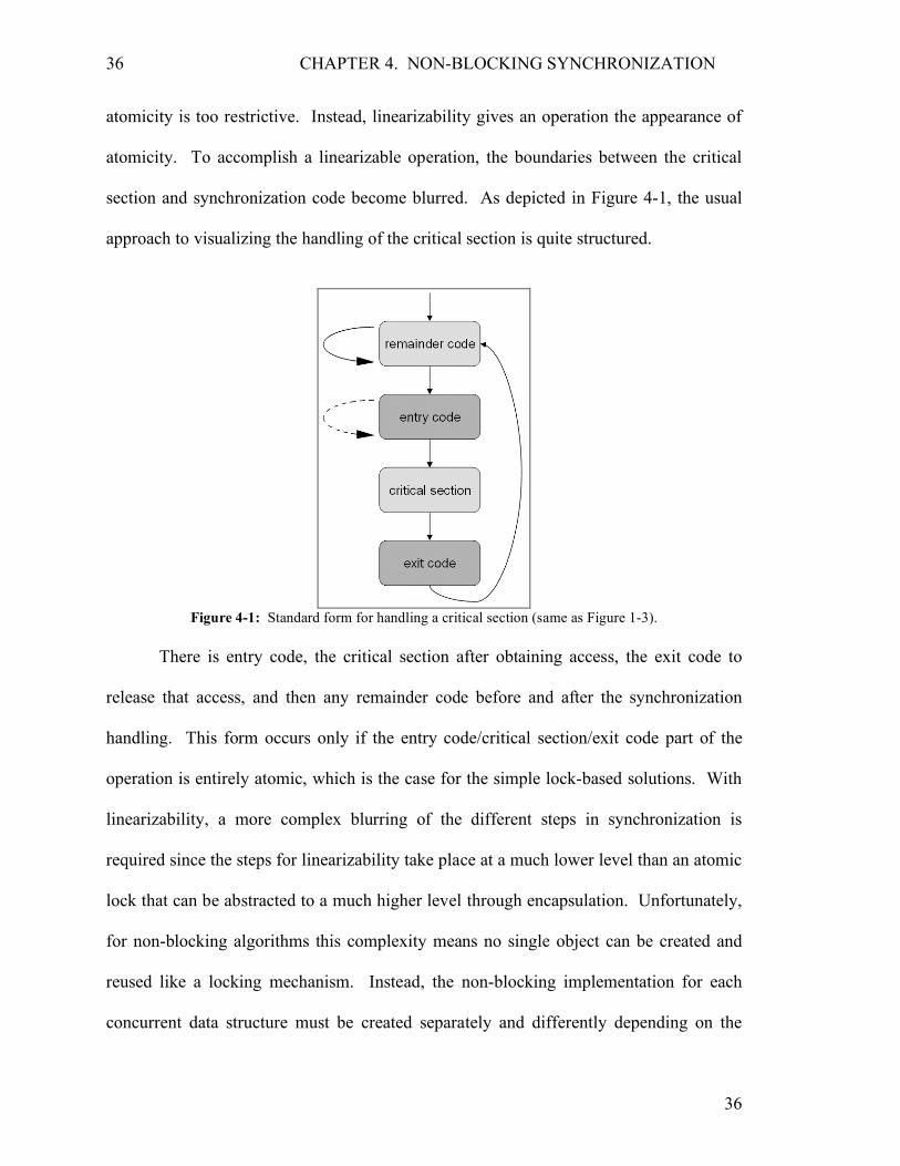
CHAPTER 4. NON-BLOCKING SYNCHRONIZATION
36
36
atomicity is too restrictive. Instead, linearizability gives an operation the appearance of
atomicity. To accomplish a linearizable operation, the boundaries between the critical
section and synchronization code become blurred. As depicted in Figure 4-1, the usual
approach to visualizing the handling of the critical section is quite structured.
Figure 4-1: Standard form for handling a critical section (same as Figure 1-3).
There is entry code, the critical section after obtaining access, the exit code to
release that access, and then any remainder code before and after the synchronization
handling. This form occurs only if the entry code/critical section/exit code part of the
operation is entirely atomic, which is the case for the simple lock-based solutions. With
linearizability, a more complex blurring of the different steps in synchronization is
required since the steps for linearizability take place at a much lower level than an atomic
lock that can be abstracted to a much higher level through encapsulation. Unfortunately,
for non-blocking algorithms this complexity means no single object can be created and
reused like a locking mechanism. Instead, the non-blocking implementation for each
concurrent data structure must be created separately and differently depending on the

CHAPTER 4. NON-BLOCKING SYNCHRONIZATION
37
properties of that structure. Figure 4-2 depicts the greater complexity of linearizable non-
blocking synchronization compared to standard blocking synchronization in Figure 4-1.
Figure 4-2: Linearizable non-blocking synchronization diagram for handling the critical sections.
Figure 4-2, besides illustrating a linearizable operation, also depicts the general
form for non-blocking algorithms. Like lock-based synchronization, remainder code,
only locally important code to the process, exists before an after the operation. However,
non-blocking algorithms also contain local code that can be thought of as code that sets
up the next atomic operation. After an atomic operation is called, but before performing
the next one, certain settings have to be established. This step should be executed in local
code with local variables, instead of with shared variables, so that other processes are not
interfered with. Only at points of atomic operations, progress-bound steps, should shared
variables be accessed. As mentioned, this is done to avoid unanticipated conflicts with

CHAPTER 4. NON-BLOCKING SYNCHRONIZATION
38
38
other processes; but also, local code optimizes variable accesses, since local variables are
read and written much faster than shared variables [12, p. 97].
Of course, the most important part of the non-blocking critical section framework
is each atomic operation. If the atomic step fails, the entire operation is restarted back at
the first local step. On successes, the next atomic step is attempted, until finally the
entire operation is completed.
Each of the atomic steps in the operation can also be implemented with
linearizable definitions, but at some point, an atomic step reaches such a primitive level
that no software-based implementation can handle such low-level atomicity. Neither the
basic test-and-set nor the newer and more complicated compare-and-swap is enough to
fully handle most non-blocking algorithms. Theoretical and hard-to-implement
hardware-based atomic operations are required to meet the needs of non-blocking
algorithms.
4.3 The ABA Problem
The atomic operation compare-and-swap would seem enough to handle most
algorithms that require exclusive access to a compare operation and then a swap
operation in a single atomic step. However, with the introduction of the compare-and-
swap instruction in the IBM System 370, the issue of the ABA problem was first reported
[6].
The ABA problem, with two processes P1 and P2 and a shared variable V that is
assigned a value of A, works as follows: If P1 reads that V is A, and then before it
executes a compare-and-swap, P2 assigns B to V, and then immediately reassigns A back

CHAPTER 4. NON-BLOCKING SYNCHRONIZATION
39
to V, the ABA problem arises. For P1, compare-and-swap will complete successfully,
since it will read A for the comparison, even though the value of V actually changed
twice before that read occurred. Thus, the ABA problem can lead to inconsistent
variables and objects that can potentially corrupt a concurrent data structure such that a
process will trap or terminate unexpectedly.
The reason why ABA is a problem can be difficult to understand since if the value
is back to A, why does it matter if it was assigned to B beforehand? Suppose that you are
an employee asked to monitor the number of people in a room. You’re told that if the
number exceeds a maximum capacity, you are a supposed to immediately notify your
boss, or else you will be fired. It just so happens that your boss is monitoring the room as
well. You’re continually watching, but sometimes you divert your eyes away with
boredom. One time, while you’re looking away, a person enters the room, breaching the
maximum number of people allowed, and then immediately leaves. You turn back and
comfortably believe that the maximum was never reached. However, your boss has
infinite patience and observed what happened, so you get fired thinking you were
cheated. This silly but simple example of the ABA problem illustrates that if a certain
state is not recognized, condition-waiting processes might not be able to proceed
correctly.
There are a few solutions to the ABA problem, but none are fully usable because
of inherent difficulties in implementing such operations in hardware architecture. A
well-known solution is called DCAS, or double-compare-and-swap. Along with variable
V, a counter or tag is attached to V to keep track of the number of times that V has been
altered. DCAS, unlike CAS (compare-and-swap), will make two comparisons, one with
CHAPTER 4. NON-BLOCKING SYNCHRONIZATION
40
40
the actual value of V, and then one with the expected value of its tag. The pseudo-code
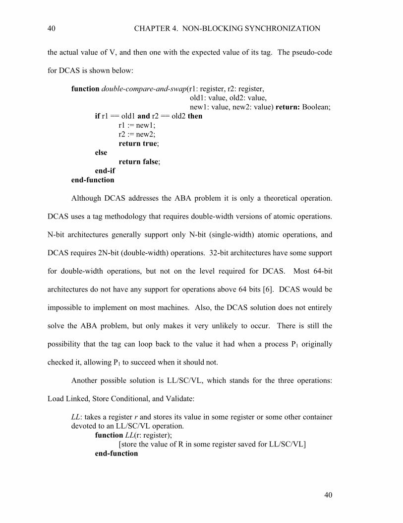
for DCAS is shown below:
function double-compare-and-swap(r1: register, r2: register, old1: value, old2: value, new1: value, new2: value) return: Boolean;
if r1 == old1 and r2 == old2 then r1 := new1; r2 := new2; return true;
else return false;
end-if end-function Although DCAS addresses the ABA problem it is only a theoretical operation.
DCAS uses a tag methodology that requires double-width versions of atomic operations.
N-bit architectures generally support only N-bit (single-width) atomic operations, and
DCAS requires 2N-bit (double-width) operations. 32-bit architectures have some support
for double-width operations, but not on the level required for DCAS. Most 64-bit
architectures do not have any support for operations above 64 bits [6]. DCAS would be
impossible to implement on most machines. Also, the DCAS solution does not entirely
solve the ABA problem, but only makes it very unlikely to occur. There is still the
possibility that the tag can loop back to the value it had when a process P1 originally
checked it, allowing P1 to succeed when it should not.
Another possible solution is LL/SC/VL, which stands for the three operations:
Load Linked, Store Conditional, and Validate:
LL: takes a register r and stores its value in some register or some other container devoted to an LL/SC/VL operation.
function LL(r: register); [store the value of R in some register saved for LL/SC/VL] end-function

CHAPTER 4. NON-BLOCKING SYNCHRONIZATION
41
SC: takes a register r and a value val. If the value of r has not changed since the last time that LL was called on it, then val is assigned to r and true is returned. Otherwise, r is left unchanged and false is returned.
function SC(r: register, val: value) return: Boolean; if [r has not changed since last LL] then r := val; return true; else return false; end-if end-function
VL: takes a register r. If the value of r has not changed since the last time that LL was called on it, then true is returned. Otherwise, false is returned.
function VL(r: register) return: Boolean; if [r has not changed since last LL] then return true else return false; end-function Since LL/SC/VL keeps track of whether a register’s value has been altered, code can be
executed between an LL call and a SC or VL call. This way, the consistency of a register
can be validated at the instant that modification is attempted. So, LL is used to store the
state of a register, and then once the local code has been executed to setup the
modification, an SC is used to enact the modification, but it will work only if another
process has not modified the register in the meantime. On a conflict, SC returns false to
notify the process that the operation must be restarted.
As with DCAS, a fully operational LL/SC/VL runs into problems of double-width
instructions, which are not supported by most architectures. LL/SC/VL can be
implemented with single-width CPUs, but practically, it is limited by the architecture
design. Versions of MIPS, PowerPC, and Alpha processors have implemented it [6], but
the mechanism is limited such that it can only be used by one program, and it cannot be
used multiple times through nesting. This limitation is due to the architectures only
supplying the hardware means to store the state of a single register for one process across

CHAPTER 4. NON-BLOCKING SYNCHRONIZATION
42
42
the entire system. The primary difference between DCAS and LL/SC/VL is that while
DCAS makes the ABA problem very unlikely to occur, LL/SC/VL eliminates the ABA
problem entirely.
With no common hardware-based solution to the ABA problem, implementing
full non-blocking algorithms is not possible. However, partial solutions using concepts
from both DCAS and LL/SC/VL make the algorithms possible in a limited fashion, as
will be explained in Chapter 5.
4.4 Livelock
There is one last issue that must be considered when designing lock-free
and non-blocking algorithms. Wait-free algorithms require that every process will make
progress within a finite number of steps. This eliminates the possibility of unbounded
waiting, so wait-free algorithms are starvation-free. By contrast, non-blocking
algorithms require only that some process will make progress within a finite number of
steps. This leaves the possibility that some processes might become starved, which
means that they will loop continually within the contending operation. This indefinite
state, called deadlock with lock-based algorithms, is instead called livelock with lock-free
algorithms. Whereas deadlock is a sleeping state that does not affect the CPU
performance, livelock entails live code that is being looped upon continually, which
potentially can waste CPU cycles in a busy-wait fashion. While this result can be
hazardous, the tradeoff is that at least some process is making progress, and as long as
that property holds, the process in livelock might eventually get out of it. Livelock is
potentially resolvable, whereas deadlock is a permanent halt to progress.
CHAPTER 4. NON-BLOCKING SYNCHRONIZATION
43
Just as blocking lock-based solutions have their advantages and disadvantages, so
do non-blocking lock-free solutions. To further explore the differences between the two
algorithms, Chapter 5 describes two implementations of the same data structure, one
implemented with the standard blocking solution, the other with an innovative non-
blocking approach.
45
Chapter 5 The Queue
In order to compare the differences between blocking and non-blocking
synchronization, the two must be implemented in a similar data structure to evaluate their
performance under the same environment. Generally, a queue is the structure used to test
synchronization mechanisms because of its common usage in many applications, whether
hardware-based or software-based. This chapter defines the properties of the queue, as
well as two implementations of the structure: a blocking and non-blocking solution.
5.1 Queue’s Properties
The most highly studied concurrent data structure and one of the most
fundamental structures is the queue. Similar to the stack, it functions as a linear structure
storing objects, but unlike the stack, which is a LIFO-based structure (Last-In First-Out),
the queue operates on a FIFO-based mechanism (First-In First-Out). Elements can be
added at any time and are generally referred to as being inserted onto the rear of the
queue, forming a line of elements with the last-inserted element at the end of the line. If
the queue is not empty, an element can be removed from the front of the line; that
element being the one in the line the longest, and therefore, at the front. Insertion is

CHAPTER 5. THE QUEUE
46
usually referred to as enqueue, while removal is referred to as dequeue [1, p. 170]. The
queue is usually conceptualized as being implemented with nodes, but it can be designed
with a circular array. A queue can use a dummy node or NULL itself to designate
whether the queue is empty or not.
Figure 5-1: Diagram of a queue’s structure, and where enqueue and dequeue take place.
Queues can be implemented at the lower level of the system architecture or at the
higher level as a software-based algorithm. For instance, differing forms of the queue are
used by the operating system to schedule processes and threads to the CPU. The round
robin scheduler acts primarily using a queue; a process is dequeued to run on the CPU for
a specific amount of time before being put back onto the queue [1, p. 176]. It then sits in
line until it reaches the front to be processed again. Queues are also used for messaging
systems so that messages are received and processed in the proper order [10, p. 892].
Resource allocation can also be implemented with a queue, an example being an
implementation of a Java Virtual Machine that could use a queue to allocate memory on
the heap [1, p. 179]. For a more detailed analysis of the possible functions/methods of a
queue, Java’s java.util.Queue is a super interface of many different queue
implementations [11].

CHAPTER 5. THE QUEUE
47
5.2 A Blocking Queue
A blocking queue can be implemented in a few different ways. The general
approach is to use a single mutex as a lock for all functions on that queue. However, a
two-lock implementation can also be designed such that each lock is reserved only for
enqueue or dequeue. A standard implementation for a single blocking mutex queue is
defined below. The queue is node-based, and to designate the empty queue, NULL is
used instead of a dummy node. For the sake of readability, the implementation is
described using pseudo-code.
Figure 5-2: A blocking queue’s declarations and initialization function.
Three structures are used in this design. The first, mutex_t, is the mutex data type,
which is assumed to be a blocking mutex as defined in Chapter 3. The structure node_t is
a single node that has two variables: a value of the data type to be stored, and a next
pointer, which will point to the next node in the line. Back in Figure 5-1, the next
pointers are the arrows from each node to the next node in the line towards the rear of the
queue. The last structure, queue_t, is the queue itself, which has three variables—
pointers to the head and tail, and a mutex instance. The initialization function sets head
and tail to NULL, the designator for an empty queue, and then initializes the mutex to an
unlocked state.

CHAPTER 5. THE QUEUE
48
Figure 5-3: A blocking queue’s enqueue function.
The function enqueue, shown in Figure 5-3, takes two parameters: a pointer to the
queue, and the value that is being inserted at the tail of the queue. It returns nothing.
Enqueue first locks the mutex to ensure that the following lines of code are executed in a
mutually exclusive manner. It creates a new node that contains the provided value. If the
queue is empty, it assigns both the head and tail to the new node (since the single node in
the queue is both the head and the tail of the queue). If the queue is not empty, it adds the
new node to the rear of the queue and sets the tail to the new node. Once the operation is
complete, the mutex must be unlocked since if the operation were to finish without
releasing the lock, a deadlock could occur the next time an enqueue or dequeue occurred
on that same queue. Thus, it unlocks the mutex to allow any other concurrent operations
to wake up and move forward.

CHAPTER 5. THE QUEUE
49
Figure 5-4: A blocking queue’s dequeue function.
The function dequeue, shown in Figure 5-4, also takes two parameters: a pointer
to the queue and a pointer to a value that will receive the dequeued value from the front
of the queue. It returns TRUE if the dequeue succeeds and FALSE otherwise. Like the
enqueue operation, the queue’s mutex must be first locked in order to ensure mutually
exclusive access to the queue. Depending on the implementation and how the queue is
used, the first steps in a dequeue operation (lines D2 through D5) may or may not be
used. They simply check the queue to see if it is empty or not. If empty, some type of
error is reported, either through a trap/exception or by returning some error-notifying
value. What is important about those steps is that if there is an error, the mutex must be
unlocked before exiting the function. Otherwise, further operations will deadlock. If the
queue is not empty, the function proceeds by storing the value of the head node into
pvalue. It then moves the head to the next node in the line and frees the old head from
memory. One last check must be done to see if the head is now NULL. If so, this means
that the queue is now empty, so to make sure that the queue is consistent, it sets the tail to
NULL as well, since otherwise it would be pointing to the freed node. To finish, as in

CHAPTER 5. THE QUEUE
50
enqueue, it unlocks the queue’s mutex to allow another concurrent operation to make
progress.
A blocking queue’s implementation is quite simple and easy to visualize. The
first process to pass the mutex’s lock call is given access to the critical section. All
subsequent processes will block; moved to the waiting state to wait for their turn to
access the queue. The blocking mutex ensures that the operations are performed as
atomic critical sections, so multiple pointer manipulations can be performed without
clobbering those pointers.1 Thus, within each function, each action moves towards
completing the operation. The blocking design provides a single critical section that is
linear in nature, and is thus linked to the same steps described in an abstract diagram of a
queue’s operations.
5.3 A Lock-Free Queue
The following lock-free queue implementation was designed by Maged M.
Michael and Michael L. Scott of the Department of Computer Science at the University
of Rochestor [7]. It uses a singly-linked list with head and tail pointers. Unlike the
blocking queue design in the previous section, a dummy node is used that head always
points to. The queue’s tail points to either the second to last or last node in the queue. In
order to ensure that dequeued nodes can be freed safely, the tail never points to any
predecessors of the second to last node. Abstractly, the atomic operation used for the
mutually exclusive operations on the pointers for each node is double-compare-and-
1 Clobbering refers to when data is overwritten while the previous contents in that data are still being used. So, a process conflict can cause pointer clobbering if one process overwrites a pointer while that pointer’s original value is still used by another process.
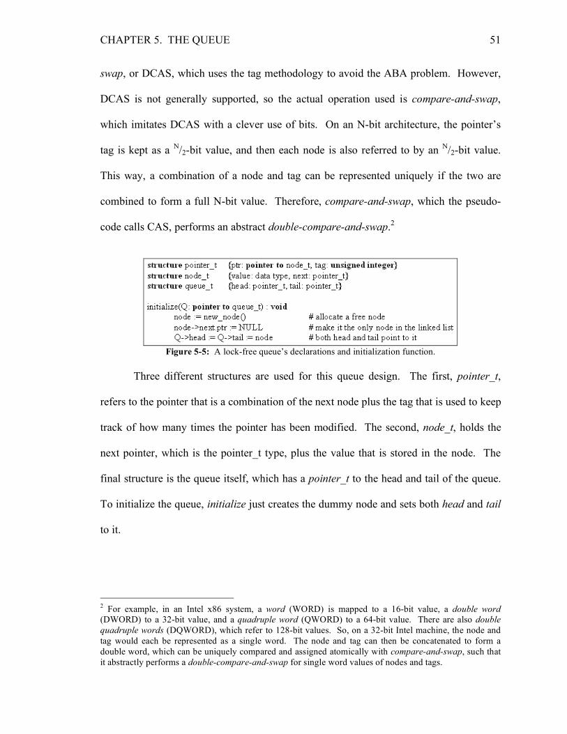
CHAPTER 5. THE QUEUE
51
swap, or DCAS, which uses the tag methodology to avoid the ABA problem. However,
DCAS is not generally supported, so the actual operation used is compare-and-swap,
which imitates DCAS with a clever use of bits. On an N-bit architecture, the pointer’s
tag is kept as a N/2-bit value, and then each node is also referred to by an N/2-bit value.
This way, a combination of a node and tag can be represented uniquely if the two are
combined to form a full N-bit value. Therefore, compare-and-swap, which the pseudo-
code calls CAS, performs an abstract double-compare-and-swap.2
Figure 5-5: A lock-free queue’s declarations and initialization function.
Three different structures are used for this queue design. The first, pointer_t,
refers to the pointer that is a combination of the next node plus the tag that is used to keep
track of how many times the pointer has been modified. The second, node_t, holds the
next pointer, which is the pointer_t type, plus the value that is stored in the node. The
final structure is the queue itself, which has a pointer_t to the head and tail of the queue.
To initialize the queue, initialize just creates the dummy node and sets both head and tail
to it.
2 For example, in an Intel x86 system, a word (WORD) is mapped to a 16-bit value, a double word (DWORD) to a 32-bit value, and a quadruple word (QWORD) to a 64-bit value. There are also double quadruple words (DQWORD), which refer to 128-bit values. So, on a 32-bit Intel machine, the node and tag would each be represented as a single word. The node and tag can then be concatenated to form a double word, which can be uniquely compared and assigned atomically with compare-and-swap, such that it abstractly performs a double-compare-and-swap for single word values of nodes and tags.

CHAPTER 5. THE QUEUE
52
Figure 5-6: A lock-free queue’s enqueue function.
Figure 5-7: A lock-free queue’s enqueue function diagram.
In the CAS operations within Figure 5-6, the third argument is constructed with a
node and tag within closing angle brackets. This symbolizes the combination of the two
N/2-bit values as a single N-bit value. The lock-free queue’s enqueue begins by first
creating the new node containing the provided value, which will be pushed onto the end
of the queue. From there, it begins to loop until the enqueue operation has completed
successfully. Recall that as a lock-free algorithm, if a synchronization conflict is
recognized, the operation is simply restarted. Local variables ltail and lnext are then
assigned the queue’s tail and next pointers respectively. The tail is first checked to see if
it has been moved since the local tail was assigned. If it is not consistent, then the
operation starts over. If the tail is consistent, it checks whether the tail is the second to
last or last node in the queue. If it is the second to last, it is up to the process to try to
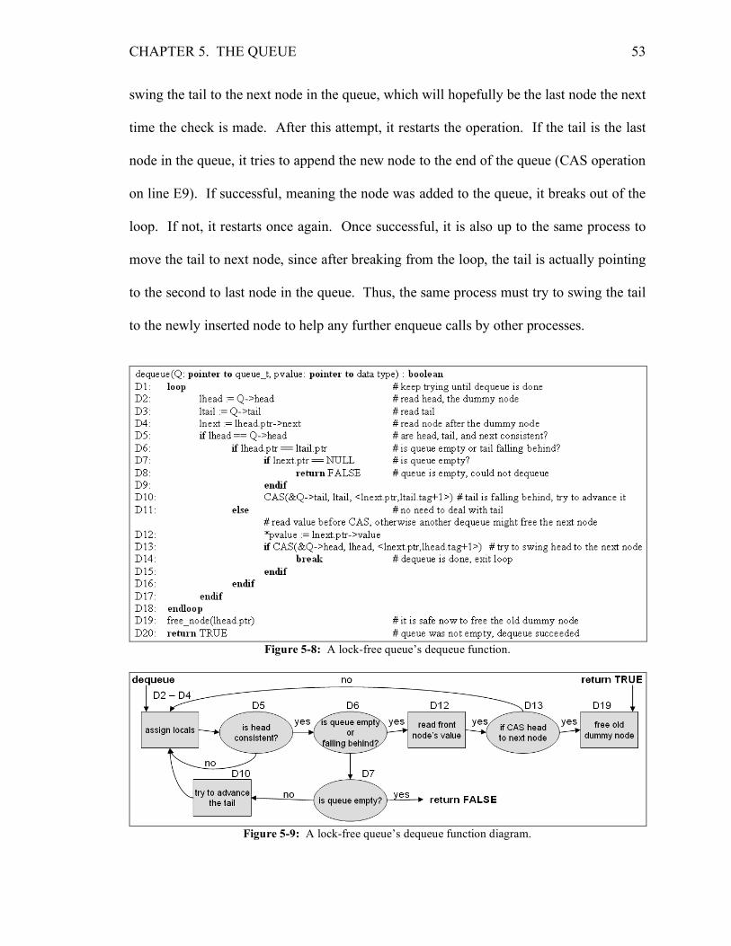
CHAPTER 5. THE QUEUE
53
swing the tail to the next node in the queue, which will hopefully be the last node the next
time the check is made. After this attempt, it restarts the operation. If the tail is the last
node in the queue, it tries to append the new node to the end of the queue (CAS operation
on line E9). If successful, meaning the node was added to the queue, it breaks out of the
loop. If not, it restarts once again. Once successful, it is also up to the same process to
move the tail to next node, since after breaking from the loop, the tail is actually pointing
to the second to last node in the queue. Thus, the same process must try to swing the tail
to the newly inserted node to help any further enqueue calls by other processes.
Figure 5-8: A lock-free queue’s dequeue function.
Figure 5-9: A lock-free queue’s dequeue function diagram.
CHAPTER 5. THE QUEUE
54
Like enqueue, dequeue also loops continually until the dequeue operation either
succeeds or fails completely; meaning the queue is empty. First, the pointer structures for
the queue’s dummy node, the front node, and the tail are assigned to the local variables
lhead, lnext, and ltail. If the queue is empty, which is when the head and tail are pointing
to the dummy and the dummy has no next node, the function simply returns FALSE to
indicate that the dequeue failed and that no value was assigned to the data type pointer. If
the head and tail are pointing to the dummy, but the dummy is not the only node in the
queue, then the queue must have exactly one element, and the tail must be pointing to the
second to last node—the dummy node. Thus, it is up to the dequeue to try and swing the
tail to the last node before restarting the operation. If the head does not equal the tail,
then a dequeue can be attempted by first storing the value of the front node, before then
trying to swing the head to the new dummy node. If successful, it breaks from the loop
and frees the old dummy node before returning TRUE to indicate that the dequeue was
successful and that there is now a valid value referenced by the data type pointer.
5.4 Linearizable and Non-Blocking
The previous lock-free queue is linearizable because at certain moments within
each operation, there is an atomic action taken such that the state of the queue is changed.
For enqueue, this takes place when the new node is attached to the end of the queue. For
dequeue, it happens when the head of the queue is moved to the next node. Lastly, the
state of the queue is never in an inconsistent or variable state. An empty queue cannot be
non-empty or vice versa. Although each method is not explicitly atomic, the queue acts
in an atomic manner, and therefore, is linearizable [7].

CHAPTER 5. THE QUEUE
55
Besides linearizable, the queue is also non-blocking because if there are multiple
processes performing operations on the queue, some process is guaranteed to complete its
operation and make progress within a finite amount of time. There are a few places in
each function where a process might fail before looping back around to start over. Each
of these places will fail only if another process is making progress, which is proven by
the following [6]:
• The condition in line E7—where the consistency of tail is tested—fails only if some other process has moved the queue’s tail forward. The tail only points to the last or second to last node in the queue, so if this condition fails more than once, that means that an enqueue was successfully completed by another process, since the current process had to move up the rear twice.
• The condition in line E8—where the tail is tested to see if it is in fact the
last node on the queue—fails only if the tail is pointing to the second to last node. Thus, the process swings the tail forward and tries again. If it fails again, this means that, like the previous condition, a successful enqueue was completed by another process.
• The compare-and-swap in line E9—where an attempt is made to append
the new node to the rear of the queue—fails if another process successfully appended its own node to the end of the queue.
• The conditions in lines D5 and D13—where the consistency of head is
checked and the actual move of the head is attempted—fail if another process successfully completed a dequeue by moving the head forward one node.
• The condition in line D6—where the queue is tested to see if it’s empty or
if the tail is falling behind—fails if another process completed a dequeue or if another process inserted its new node at the end of the queue. Thus, if this condition fails more than once, then either another dequeue occurred or an enqueue succeeded.
As evident by the Michael and Scott algorithm, the non-blocking queue
implementation is much more complicated than a simple single-mutex blocking queue.
The real test however is how well each performs, which is determined in Chapter 6.

57
Chapter 6 Blocking vs. Non-Blocking
This chapter explains the low-level implementations of the blocking queue and
the non-blocking queue defined in Chapter 5, before also discussing experiments in
which the two are run separately in a multi-threaded environment. The code, which was
written with the C programming language since C offers faster runtime execution and
more precise measurements of time, is included in the Appendix.1
6.1 Non-Blocking Queue
Before building the blocking queue (the simpler implementation) the non-
blocking queue had to be designed, so that the blocking queue could conform to the
peculiarities of the stricter implementation. For example, if the non-blocking queue uses
a stack-allocated array to contain its nodes, then the blocking queue should also use a
stack. If the blocking queue allocated its nodes on the heap, and the non-blocking queue
did not, the blocking algorithm would immediately be at a disadvantage since heap
allocation and heap lookups take more time than stack-based handling.
1 The code is loosely based upon a test provided with the code distributed by Michael and Scott [7].

CHAPTER 6. BLOCKING VS. NON-BLOCKING 58
The first step to building the non-blocking queue was creating the atomic
operation compare-and-swap. CAS is supported on most modern machines, but there is
no common API, and there is no single way to execute a CAS statement in C across
different operating systems. For example, the Win32 API contains the interlocked
function InterlockedCompareExchange, while some Unix-based machines have the
simple compare_and_swap.
The only way to ensure that the proper CAS call is made is to execute it at the
assembly level. Intel’s x86 processors support the compare-and-swap operation
CMPXCHG. Therefore, an assembly implementation with CMPXCHG is defined in
“atomic_cas.c” [Appendix, 2]. CMPXCHG supports both 32-bit and 64-bit processors,
but atomic_cas is aligned for 32-bit processing only.
The actual non-blocking queue is declared in “nb_queue.h” [Appendix, 5]. The
tag methodology is required, which means that the queue can only hold up to N/2-bit
nodes. The code is aligned for 32-bit processing, so the maximum number of nodes in
the queue is equal to the maximum possible value of an unsigned short, or 216 – 1. Thus,
the nodes are referenced by unsigned short integers rather than by 32-bit pointer values.
This in turn means that nodes cannot be created on the fly by the heap, since pointers are
32-bit values that cannot be referenced uniquely as 16-bit values. So, unique 16-bit
values must be assigned to each node, but there is no way to uniquely assign those values
without another level of atomicity to ensure that each assigned value is in fact distinct
from any others currently being used. If this step was not handled atomically, a duplicate
could be assigned such that, first, the node that the value originally pointed to will be lost

CHAPTER 6. BLOCKING VS. NON-BLOCKING 59
in a memory leak, and second, the value will reside in the queue twice while pointing to
the same node.
The solution is to use a fixed-size array of nodes where the index represents the
unsigned short identifier for the node. The array must be created at structure
initialization, either on the stack or on the heap, depending on whether dynamic sizing is
allowed. For increased speed, the array is allocated on the stack with a constant size of
MAX_NODES, which is 0xFF (256). The greatest possible maximum size would be the
largest number two bytes can represent, but a queue of size 256 is sufficient for the
comparison.
An array of nodes does not entirely solve the issue of node allocation. On an
enqueue, choosing which node on the array to “allocate” is still a non-trivial problem,
since that step needs to be atomic or seemingly atomic. Since using another level of
atomicity eliminates the point of the non-blocking queue, the solution is to have each
thread keep track of which node it will eventually add on an enqueue. This solution
requires two extra steps: First, each thread must be initialized with a node that is
guaranteed to work on the queue. Second, after an enqueue, the only way to retrieve a
valid node for another enqueue is to call a dequeue, since a dequeue will have an
available node after freeing the dummy node. A consequence of this solution is that a
dequeue cannot be executed on an empty queue, since the thread that made the call will
not receive the freed dummy node as its next valid node to enqueue with. Therefore,
once a thread has executed a dequeue on an empty queue, that thread is invalidated unless
it is reinitialized with a new valid node, or if it continues to make dequeue calls until the
queue is no longer empty.

CHAPTER 6. BLOCKING VS. NON-BLOCKING 60
The node allocation and handling scheme is implemented through the structure
local_t [Appendix, 3-4]. The structure contains a thread identifier for debugging, an
unsigned short node, an unsigned short value, and a field called backoff. The node field
keeps track of the next node to use on an enqueue. The non-blocking queue takes in a
local_t pointer with its enqueue and dequeue methods so that it can read and write the
node for the thread executing the call. For enqueues, value is the element inserted. Thus,
after every enqueue, value is incremented to provide a new value for each subsequent
enqueue.
The node allocation and handling mechanism is the most complex part about the
Michael and Scott Non-Blocking Concurrent Queue Algorithm. It is a limited
workaround for the problems caused by trying to imitate the double-compare-and-swap
operation. The only other non-trivial step in the algorithm involves ensuring that the
pointer_t structure can handle both big endian and little endian processors and that when
combining two 16-bit values into a 32-bit value, it is done properly.
The non-blocking queue also optionally uses an exponential backoff approach for
threads that run into conflicts. When a thread encounters a conflict, if backoff is enabled,
the thread will iterate a certain amount of times before starting over to try to back away
from aligned conflict looping. Aligned conflict looping refers to two or more threads
continually conflicting because they are stuck running side-by-side in more or less the
exact order of executing atomic operations. Exponential backoff can be implemented
both as constant exponential backoff or instead as pseudo-random exponential backoff.2
2 The difference between the two exponential backoff approaches is as follows: constant exponential backoff means that the backoff is incremented by a power of 2, and then that amount is used as the backoff iteration in the next backoff call. For pseudo-random exponential backoff, that new amount is used as the maximum for determining a random backoff to iterate by.

CHAPTER 6. BLOCKING VS. NON-BLOCKING 61
In the local_t structure, the backoff field keeps track of the current backoff for the thread.
The default behavior for the queue is to disable exponential backoff.3
6.2 Blocking Queue
The blocking queue is implemented using the standard node-based mechanism,
with its operations surrounded by a single mutex to ensure mutual exclusion. To keep the
two queue implementations as similar as possible, the queue is initialized with a fixed-
size array of nodes allocated on the stack, keeping a comparable allocation speed between
the two queues. The blocking queue also uses the local_t structure to keep the calls
between the queues the same as well. Besides these changes, the blocking queue remains
the same as any standard blocking node-based queue. The only real difference between
the two queues is the blocking and non-blocking mechanisms.
6.3 Barrier and Statistics
There are two other sets of files: “barrier.h” and “simstat.h,” along with their
associated source files. “barrier.h” contains a declaration for a barrier implementation
called barrier_t [Appendix, 9]. It supports the basic barrier mechanism, which keeps
threads blocked until a certain party threshold has been reached. For this
implementation, an additional requirement must be met before the threads are released.
A release call has to be made explicitly by a controlling thread. This allows the barrier to
be monitored from a context not blocked by the barrier, providing a way to determine
exactly when the threads on the barrier are released. The barrier is also designed to
3 Unless stated otherwise, it should be assumed that exponential backoff is not being used.
CHAPTER 6. BLOCKING VS. NON-BLOCKING 62
prevent mixing barrier calls. This helps make sure that threads do not break from one
barrier and then enter another, only to conflict with the previous barrier. When a thread
is released from a barrier, it cannot enter another barrier using the same instance without
all threads having first been released by the previous barrier. The structure barrier_t is
used extensively to control the threads running in the simulation.
The second set of files, “simstat.h” and its source file [Appendix, 11-12], is a bit
more complicated. It provides the means to handle tracking statistics for each thread and
simulation. Depending on the system however, tracking performance is non-trivial. The
code supports two compilations to support the two different implemented types of
recording time: clock ticks and real-time nanoseconds. Nanosecond precision is obtained
from the Linux real-time library4 through the function call clock_gettime.
On a single processor machine, real-time is an inaccurate way to judge execution
time due to context switching. Clock ticks are better suited for the task, but only for
comparing time, not for acquiring actual time statistics. The standard C call clock5
returns the number of clock ticks from an arbitrary point in time. Thus, a start time and
an end time can be used to determine how many clock ticks have passed in an interim
period. The number of clock ticks is only calculated based on when the process is on the
CPU. There are about a million clock ticks per second, so running code for sixty million
clock ticks (one minute) will take a little longer than a minute to complete the execution,
since context switches that occur within that time period prevent the number of clock
ticks to accurately reach one minute in real-time. The simulation uses threads rather than
processes, so if a process is context-switched off the CPU, then all of its threads are.
4 This only works on Linux, and when compiled, it must be linked with “-lrt”. clock_gettime is declared in the standard C header <time.h>. 5 Also declared in <time.h>, but included in all C distributions.

CHAPTER 6. BLOCKING VS. NON-BLOCKING 63
Thus, they remain in the same state, and a comparison between their completion times
can still be computed. The conversion from clock ticks to real-time can be estimated, but
because the same estimation approach is applied to both the blocking and non-blocking
queues, the comparison between the two remains accurate. Thus, if one queue consumes
more clock ticks than another to complete a certain operation, it is safe to say that that
queue takes longer in real-time than the other queue.6
6.4 The Simulation
The actual simulation code is defined in “main.c” [Appendix, 13], which handles
the blocking and non-blocking queues separately, depending on whether the
NON_BLOCKING macro has been defined. The main thread generates a number of
child threads (the default number of child threads is one hundred). The threads run up
against a barrier to prevent them from continuing until every thread has been created.
Once all are created, they are released by the main thread. They then try to pass through
a synchronization bottleneck, where multiple iterations of enqueues and dequeues take
place on the shared queue (default is 10,000 per thread). The bottleneck encourages as
many conflicts as possible between threads. Between each enqueue and dequeue there is
a loop of empty work (blank statements) consisting of, by default, a thousand iterations.
The empty work is there to encourage thread-based context switches between enqueues
and dequeues. Before each child thread enters the bottleneck, a start time is recorded.
Once it has left, an end time is recorded before immediately stopping at another barrier.
6 The difference between real-time and clock ticks was tested on Linux using a few lines of code to compare a certain amount of clock ticks against the actual amount of time that had passed. While the code is running, other programs were accessed and used, causing further context switches. The difference showed that, at least for that version of Linux, the number of clock ticks measured is only for the currently running process.

CHAPTER 6. BLOCKING VS. NON-BLOCKING 64
This way, no extra code is executed while the iterations are taking place; otherwise, that
extra code would affect the results of the threads still trying to pass the bottleneck. Once
all threads have completed their passes, their times are gathered into one common
structure, a simstat_t structure, which the main thread can use to calculate the statistics
for the simulation: the maximum, minimum, mode, median, mean, and standard
deviation. Once calculated, the results are recorded, and the next simulation begins—
with more simulations, the more accurate the results since each simulation can be used to
compute an overall average set of statistics.
The makefile [Appendix, 14] for the experiment provides two configurations.
“clock,” for testing the blocking and non-blocking queues by measuring clock ticks, and
“rt,” for testing the blocking and non-blocking queues by measuring nanoseconds.
6.5 Results
The following tests were completed with a default setting of 10,000 iterations of
enqueues and dequeues, and 1,000 iterations of empty work between each operation.
They were run on two machines, a single Intel 32-bit processor system and a four
AMD64 dual core multiprocessor system.
The first set of tests was performed to verify the simple difference in overhead
between the blocking and non-blocking queues. On the single processor machine,
running a test of one thread for a thousand simulations produced the following results:
For blocking, the thread, on average, completed the bottleneck in about 17,130 clock
ticks, or about 17.13 milliseconds. For non-blocking it completed in about 16,410 clock
ticks, or about 16.41 milliseconds. On the multiprocessor machine, the same two tests
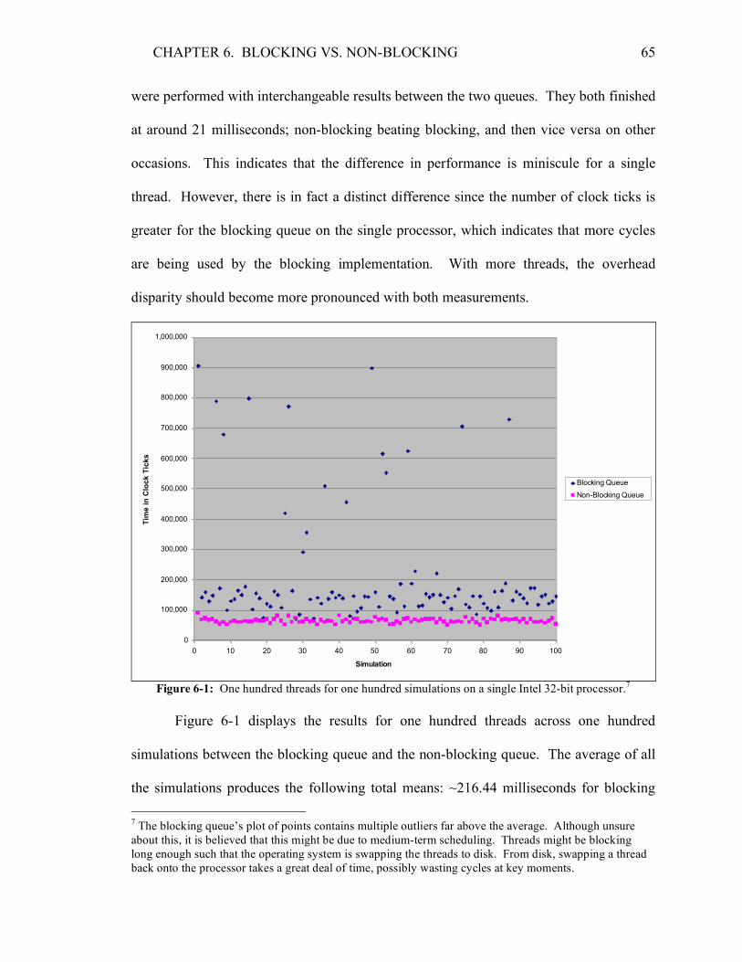
CHAPTER 6. BLOCKING VS. NON-BLOCKING 65
were performed with interchangeable results between the two queues. They both finished
at around 21 milliseconds; non-blocking beating blocking, and then vice versa on other
occasions. This indicates that the difference in performance is miniscule for a single
thread. However, there is in fact a distinct difference since the number of clock ticks is
greater for the blocking queue on the single processor, which indicates that more cycles
are being used by the blocking implementation. With more threads, the overhead
disparity should become more pronounced with both measurements.
0
100,000
200,000
300,000
400,000
500,000
600,000
700,000
800,000
900,000
1,000,000
0 10 20 30 40 50 60 70 80 90 100
Simulation
Tim
e i
n C
loc
k T
ick
s
Blocking Queue
Non-Blocking Queue
Figure 6-1: One hundred threads for one hundred simulations on a single Intel 32-bit processor.7
Figure 6-1 displays the results for one hundred threads across one hundred
simulations between the blocking queue and the non-blocking queue. The average of all
the simulations produces the following total means: ~216.44 milliseconds for blocking
7 The blocking queue’s plot of points contains multiple outliers far above the average. Although unsure about this, it is believed that this might be due to medium-term scheduling. Threads might be blocking long enough such that the operating system is swapping the threads to disk. From disk, swapping a thread back onto the processor takes a great deal of time, possibly wasting cycles at key moments.

CHAPTER 6. BLOCKING VS. NON-BLOCKING 66
and ~65.31 milliseconds for non-blocking. Although converting clock ticks into
milliseconds is merely an estimate, the difference between the two stats is accurate. This
indicates that non-blocking performs much better in a multiprogramming environment on
a single processor.
0.00E+00
1.00E+08
2.00E+08
3.00E+08
4.00E+08
5.00E+08
6.00E+08
7.00E+08
8.00E+08
9.00E+08
1.00E+09
1.10E+09
1.20E+09
1.30E+09
1.40E+09
1.50E+09
1.60E+09
0 10 20 30 40 50 60 70 80 90 100
Simulation
Tim
e (
nan
oseco
nd
s)
Blocking Queue
Non-Blocking Queue
Figure 6-2: One hundred threads for one hundred simulations on four AMD64 multiprocessors.
Using the previous test again on the multiprocessor machine, Figure 6-2 depicts
the difference in performance between the blocking and non-blocking implementations.
Measured in real-time at a precision of nanoseconds, non-blocking took about 29.47
milliseconds, whereas blocking took about 1520.38 milliseconds, or over 1.5 seconds to
complete. The results show that, as with the single processor, the non-blocking queue

CHAPTER 6. BLOCKING VS. NON-BLOCKING 67
algorithm is much faster than the regular blocking queue algorithm on a multiprocessor
machine.8
A final test was performed on each machine to determine the effect an
exponential backoff algorithm would have on resolving conflicts at the synchronization
bottleneck for the non-blocking queue. Both the regular exponential backoff and the
pseudo-random exponential backoff algorithms were tested. All three algorithms,
including the normal non-blocking queue, performed about the same on both machines.
This raises the question of how many conflicts are actually occurring in the bottleneck
using the non-blocking queue. It seems to make sense that more conflicts would lead to a
greater difference in the results, but they are instead very similar. This suggests that the
assumption of lock-free algorithms that conflicts between processes or threads are rare is
an accurate one.
8 It is important to mention that the exact numbers are not consistent across multiple tests due to differing testing environments: the computer, the processes running, the users logged in, etc. However, across all tests, the difference between the blocking queue and the non-blocking queue remains consistent.

69
Chapter 7 Conclusion
Blocking synchronization is the status quo for synchronizing shared memory
across processes or threads on a single system. It puts a process to sleep in order to
prevent a busy-wait or spinlock. This conserves CPU cycles, allowing other progress-
bound processes to move forward. Lock-based synchronization ensures that the critical
sections are executed in a mutually exclusive manner so that no data becomes corrupted
or inconsistent. Blocking synchronization is easy to code with since it can be
encapsulated in objects such as semaphores, mutexes, monitors, and reader-writer locks.
These objects also provide reusability, which is often paramount in a programmer’s
solution choice. Lastly, blocking synchronization provides the option of a fair policy
implementation, in which processes are ordered fairly and executed based upon their
arrival times.
Nevertheless, blocking has some disadvantages. It requires a great deal of
overhead. The blocking and wakeup calls, which involve interacting with the operating
system, require time to process. The maintenance of the fair policy requires additional
time and space. Any locked-based algorithm must deal with the problem of deadlock. If
deadlock occurs, the process can fail. Lastly, due to the overhead, the requirement of
CHAPTER 7. CONCLUSION 70
mutual exclusion, and the property of fairness blocking synchronization can be quite
slow.
Non-blocking synchronization is a newer alternative synchronization that seeks to
resolve some of the issues inherent in lock-based algorithms. Non-blocking has little
overhead since it does not worry about blocking, waking, or maintaining a mechanism for
a fair policy. Without that mechanism, less time and space is used. Non-blocking
algorithms are a subset of lock-free algorithms, and hence, they do not have to deal with
deadlock. If a process fails in the critical section, the other processes do not also fail.
Instead, they continue with progress, as intended. Under the assumption that conflicts
between processes are actually rare, non-blocking algorithms do not waste time with
cautionary measures. As indicated by the results in Chapter 6, non-blocking is the faster
algorithm.
Despite the apparent speed of non-blocking synchronization, it has some severe
limitations. First, although both blocking and non-blocking do not satisfy starvation-
freedom, non-blocking does not guarantee fairness, whereas blocking does. Second,
livelock is an issue of non-blocking lock-free algorithms. Instead of getting stuck in the
inactive state of deadlock, livelock can potentially be more hazardous since it is an
indefinite state where live code is being executed. However, it should be noted that, in
practice, the situation does not occur often, and even then, livelock is not permanent.
Third, there is the ABA problem, which is inherent to any system architecture using the
atomic compare-and-swap operation. No system fully supports an operation such as
double-compare-and-swap or LL/SC/VL to facilitate a complete implementation of many
non-blocking algorithms. The complexity of the Michael and Scott Non-Blocking

CHAPTER 7. CONCLUSION 71
Concurrent Queue Algorithm attests to the difficulty in implementing a non-blocking
algorithm with modern architectures, even for a simple data structure such as the queue.
Despite the fact that it works, the implementation is rigoursly limited in many respects.
Perhaps most significantly, non-blocking synchronization must be implemented on a
case-by-case basis. Thus, the algorithms are not only more complex, but also not
reusable—a programmer’s worst nightmare. Currently, the only widely used
implementation of a non-blocking algorithm is in Sun’s distribution of Java 5, which
includes the class java.util.concurrent.ConcurrentLinkedQueue [8]. The queue
implements the Michael and Scott algorithm; however, the ABA problem is not handled
at all. In many respects, the ABA problem is the primary reason why non-blocking
algorithms are so difficult to implement.
All in all, non-blocking synchronization is an innovative step, but it is still strictly
lacking. However, such algorithms should still be considered for special cases, i.e.,
databases or programs designed specifically for multiprocessor environments.
Otherwise, blocking synchronization should be the continued solution of choice for most
other purposes. Its power lies in its ease of use and reusability through encapsulated
objects. For most applications, blocking synchronization can be utilized without any
noticeable sacrifice in performance.
Without a significant leap in system architecture capabilities, non-blocking
algorithms will continue to be the second choice in process and thread synchronization.
73
Appendix (Source Code) A.1 atomic_cas.h /* Kevin Chirls * Senior Thesis in Computer Science * Middlebury College 2007 * * Atomic Compare-And-Swap for 32-bit values only (Header) */ #ifndef _ATOMIC_CAS_H_ #define _ATOMIC_CAS_H_ /* Compare-And-Swap * * If the value pointed to by the pointer (dest) is equivalent to the * expected value (expected), then the value of the pointer is replaced * with a new value (replacement). Upon success, 1 for true is returned, * otherwise 0 for false. */ int atomic_cas(void *dest, int expected, int replacement); #endif /* _ATOMIC_CAS_H_ */
A.2 atomic_cas.c /* Kevin Chirls * Senior Thesis in Computer Science * Middlebury College 2007 * * Atomic Compare-And-Swap for 32-bit values only (Source) */ #include "atomic_cas.h" int atomic_cas(void *dest, int old, int new) { char retval; __asm__ __volatile__ ("lock; cmpxchgl %2, %0; setz %1" : "=m"(*(int*)dest), "=a"(retval) : "r" (new), "a"(old), "m"(*(int*)dest) : "memory"); return retval; }

APPENDIX 74
A.3 local.h /* Kevin Chirls * Senior Thesis in Computer Science * Middlebury College 2007 * * Structure to handle all members related to the queue that are local * to the thread that is calling the queue function (Header) * * Note that this uses an expenential backoff algorithm, which uses * three variables "backoff_base", "backoff_append", and "backoff_cap". * When "backoff_delay" is called, the thread will loop for: * 2^(l->backoff) - 1 * Once done, l->backoff is incremented by the backoff_append. The max * backoff can be is backoff_cap. The initial backoff for each local * structure is set to backoff_base. * * backoff_base, backoff_cap, and backoff_append should be defined in main.c. * backoff_on and backoff_rand should also be defined in main.c, but they act * as boolean integers instead of values used in the algorithm. */ #ifndef _LOCAL_H_ #define _LOCAL_H_ typedef struct _local { long int thread; /* for debugging */ unsigned short node, value; unsigned short backoff; } local_t; /* initializes the local structure to the provided thread */ void local_init(local_t *l, long int thread, unsigned short initial_nodes, unsigned short iterations); /* Runs an exponential increasing backoff delay */ void local_backoff_delay(local_t *l); /* Clears the backoff to the initial base value */ void local_backoff_clear(local_t *l); /* Use this to print an error message to STDERR, before exiting the thread. * Be careful!!! Any memory still allocated to the heap will be left there! */ void local_exit(local_t *l, const char *err_msg); #endif /* _LOCAL_H_ */

APPENDIX
75
A.4 local.c /* Kevin Chirls * Senior Thesis in Computer Science * Middlebury College 2007 * * Structure to handle all members related to the queue that are local * to the thread that is calling the function (Source) */ #include "local.h" #include <sys/types.h> /* always included before all unix headers */ #include <pthread.h> /* Posix threads */ #include <stdlib.h> /* for rand() */ #include <stdio.h> /* fprintf, stderr */ /* defined in "main.c" */ extern unsigned int backoff_base; extern unsigned int backoff_cap; extern unsigned int backoff_append; extern int backoff_rand; extern int backoff_on; void local_init(local_t *l, long int thread, unsigned short initial_nodes, unsigned short iterations) { l->thread = thread; l->node = 2 + initial_nodes + thread; l->value = 1 + initial_nodes + (thread * iterations); l->backoff = backoff_base; } void local_backoff_delay(local_t *l) { unsigned int i = 0, b; if (backoff_on) { if (backoff_rand) b = rand() % ((1 << l->backoff) - 1); else b = (1 << l->backoff) - 1; while (i < b) i++; /* backoff */ if (l->backoff < backoff_cap) { l->backoff += backoff_append; if (l->backoff > backoff_cap) l->backoff = backoff_cap; } } } void local_backoff_clear(local_t *l) { l->backoff = backoff_base; }
APPENDIX 76
void local_exit(local_t *l, const char *err_msg) { int status = 1; fprintf(stderr,"Thread %ld Terminated: %s\n",l->thread,err_msg); pthread_exit(&status); }
A.5 nb_queue.h /* Kevin Chirls * Senior Thesis in Computer Science * Middlebury College 2007 * * Non-Blocking Queue (Header) * * Based on the Michael and Scott Non-Blocking Concurrent Queue Algorithm. * The code has also been taken from their distribution and has been slightly * modified. * * Note that if the queue is "dequeued" while the queue is empty, then the * thread that made the call will no longer be able to use the queue. */ #ifndef _NB_QUEUE_H_ #define _NB_QUEUE_H_ #include <stdlib.h> /* for LITTLE_ENDIAN */ #include "local.h" /* thread local structure */ /* 256 possible nodes (max for threads as well). * This could be up to the maximum size for an unsigned short, but might * as well be smaller, since I'm not going to use a queue of that size. */ #define MAX_NODES 0xFF /* a 32 bit pointer that is identified by a 16 bit value and a 16 bit tag */ typedef union _pointer { struct { /* A GNU gcc bug causes BIG_ENDIAN to be defined on x86 machines, so use LITTLE_ENDIAN only */ #ifdef LITTLE_ENDIAN volatile unsigned short ptr; volatile unsigned short tag; #else volatile unsigned short tag; volatile unsigned short ptr; #endif }; volatile unsigned long id; } pointer_t; /* a node in the queue */

APPENDIX
77
typedef struct _node { unsigned int value; pointer_t next; } node_t; /* the queue */ typedef struct _queue { pointer_t head, tail; node_t nodes[MAX_NODES + 1]; } queue_t; /* Initializes the queue */ void queue_init(queue_t *Q, unsigned short initial_nodes); /* Destroys the queue (nothing to destroy for NB queue) */ #define queue_destroy(Q) /* Takes the local value stored in the thread local structure and adds * it to the end of the queue. The value in the local structure is * incremented by 1. */ void queue_enqueue(queue_t *Q, local_t *l); /* Removes and returns the value from the front of the queue. If the queue * is empty, unlike the blocking queue, this method will immediately * terminate the thread... A dequeue on an empty queue with this implementation * causes the thread's local structure to become corrupt. The thread is then * useless, and will potentially corrupt the whole queue or will cause a * segmentation fault. So, the thread is immediately destroyed. */ unsigned short queue_dequeue(queue_t *Q, local_t *l); #endif /* _NB_QUEUE_H_ */
A.6 nb_queue.c /* Kevin Chirls * Senior Thesis in Computer Science * Middlebury College 2007 * * Non-Blocking Queue (Source) */ #include "nb_queue.h" #include "atomic_cas.h" /* NULL needs to be 0, not (void*)0, since the nodes are actually shorts, * not actual pointers. */ #ifdef NULL # undef NULL
APPENDIX 78
#endif #define NULL 0 /* converts a 16-bit pointer and tag into its 32-bit unique value */ # define MAKE_PTR(ptr,tag) ((tag)<<16)+(ptr) void queue_init(queue_t *Q, unsigned short initial_nodes) { unsigned int i; /* initialize queue */ Q->head.ptr = 1; Q->head.tag = 0; Q->tail.ptr = 1; Q->tail.tag = 0; Q->nodes[1].next.ptr = NULL; Q->nodes[1].next.tag = 0; /* initialize available list */ for (i = 2; i < MAX_NODES; i++) { Q->nodes[i].next.ptr = i + 1; Q->nodes[i].next.tag = 0; } Q->nodes[MAX_NODES].next.ptr = NULL; Q->nodes[MAX_NODES].next.tag = 0; /* initialize queue contents */ if (initial_nodes > 0) { for (i = 2; i < initial_nodes + 2; i++) { Q->nodes[i].value = i; Q->nodes[i - 1].next.ptr = i; Q->nodes[i].next.ptr = NULL; } Q->head.ptr = 1; Q->tail.ptr = 1 + initial_nodes; } } void queue_enqueue(queue_t *Q, local_t *l) { pointer_t l_tail, l_next; unsigned short node = l->node; Q->nodes[node].value = l->value++; Q->nodes[node].next.ptr = NULL; local_backoff_clear(l); while (1) { l_tail.id = Q->tail.id; l_next.id = Q->nodes[l_tail.ptr].next.id; if (l_tail.id == Q->tail.id) { if (l_next.ptr == NULL) { if (atomic_cas(&Q->nodes[l_tail.ptr].next,l_next.id,MAKE_PTR(node,l_next.tag + 1))) { atomic_cas(&Q->tail,l_tail.id,MAKE_PTR(node,l_tail.tag + 1)); return; } } else atomic_cas(&Q->tail,l_tail.id,MAKE_PTR(Q->nodes[l_tail.ptr].next.ptr,l_tail.tag + 1)); local_backoff_delay(l); } } }

APPENDIX
79
unsigned short queue_dequeue(queue_t *Q, local_t *l) { unsigned short value; pointer_t l_head, l_tail, l_next; local_backoff_clear(l); while (1) { l_head.id = Q->head.id; l_tail.id = Q->tail.id; l_next.id = Q->nodes[l_head.ptr].next.id; if (l_head.id == Q->head.id) { if (l_head.ptr == l_tail.ptr) { if (l_next.ptr == NULL) { local_exit(l,"Dequeued an empty NB queue"); /* kills the thread */ return NULL; } atomic_cas(&Q->tail,l_tail.id,MAKE_PTR(l_next.ptr,l_tail.tag + 1)); local_backoff_delay(l); } else { value = Q->nodes[l_next.ptr].value; if (atomic_cas(&Q->head,l_head.id,MAKE_PTR(l_next.ptr,l_head.tag + 1))) { l->node = l_head.ptr; /* reclaim (free) node */ return value; } local_backoff_delay(l); } } } }
A.7 b_queue.h /* Kevin Chirls * Senior Thesis in Computer Science * Middlebury College 2007 * * Single-Mutex Blocking Queue (Header) */ #ifndef _B_QUEUE_H_ #define _B_QUEUE_H_ #include <sys/types.h> /* always included before any other unix headers */ #include <pthread.h> /* Posix threads (for mutex) */ #include "local.h" /* thread local structure */ /* 256 possible nodes (max for threads as well). * This could be up to the maximum size for an unsigned short, but might * as well be smaller, since I'm not going to use a queue of that size. */ #define MAX_NODES 0xFF
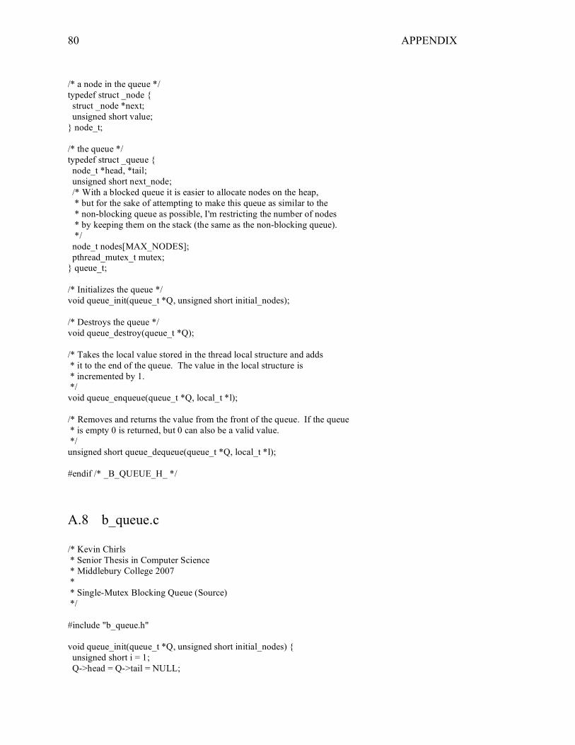
APPENDIX 80
/* a node in the queue */ typedef struct _node { struct _node *next; unsigned short value; } node_t; /* the queue */ typedef struct _queue { node_t *head, *tail; unsigned short next_node; /* With a blocked queue it is easier to allocate nodes on the heap, * but for the sake of attempting to make this queue as similar to the * non-blocking queue as possible, I'm restricting the number of nodes * by keeping them on the stack (the same as the non-blocking queue). */ node_t nodes[MAX_NODES]; pthread_mutex_t mutex; } queue_t; /* Initializes the queue */ void queue_init(queue_t *Q, unsigned short initial_nodes); /* Destroys the queue */ void queue_destroy(queue_t *Q); /* Takes the local value stored in the thread local structure and adds * it to the end of the queue. The value in the local structure is * incremented by 1. */ void queue_enqueue(queue_t *Q, local_t *l); /* Removes and returns the value from the front of the queue. If the queue * is empty 0 is returned, but 0 can also be a valid value. */ unsigned short queue_dequeue(queue_t *Q, local_t *l); #endif /* _B_QUEUE_H_ */
A.8 b_queue.c /* Kevin Chirls * Senior Thesis in Computer Science * Middlebury College 2007 * * Single-Mutex Blocking Queue (Source) */ #include "b_queue.h" void queue_init(queue_t *Q, unsigned short initial_nodes) { unsigned short i = 1; Q->head = Q->tail = NULL;

APPENDIX
81
Q->next_node = 0; if (initial_nodes > 0) { Q->nodes[0].value = 0; for (; i < initial_nodes; i++) { Q->nodes[i - 1].next = &Q->nodes[i]; Q->nodes[i].value = i; Q->nodes[i].next = NULL; } Q->head = &Q->nodes[0]; Q->tail = &Q->nodes[initial_nodes - 1]; Q->next_node = initial_nodes; } pthread_mutex_init(&Q->mutex,NULL); } void queue_destroy(queue_t *Q) { pthread_mutex_destroy(&Q->mutex); } void queue_enqueue(queue_t *Q, local_t *l) { node_t *node; pthread_mutex_lock(&Q->mutex); node = &Q->nodes[Q->next_node]; Q->next_node = (Q->next_node + 1) % MAX_NODES; node->next = NULL; node->value = l->value++; if (Q->tail) Q->tail->next = node; else Q->head = node; Q->tail = node; pthread_mutex_unlock(&Q->mutex); } unsigned short queue_dequeue(queue_t *Q, local_t *l) { unsigned short value = 0; pthread_mutex_lock(&Q->mutex); if (Q->head) { value = Q->head->value; Q->head = Q->head->next; if (!Q->head) Q->tail = NULL; } pthread_mutex_unlock(&Q->mutex); return value; }

APPENDIX 82
A.9 barrier.h /* Kevin Chirls * Senior Thesis in Computer Science * Middlebury College 2007 * * Barrier (Header) * * This barrier does not follow the general guidelines of a barrier. Instead * of releasing once the number of parties has been reached, the barrier releases * only when a call to "barrier_release" has been made. For more details look * below at the documentation. * * This barrier also prevents threads from looping back around and reentering * into a previous barrier stop call. Each stop is independently handled, and no * thread can enter another stop until every thread has been released from a previous * stop. */ #ifndef _BARRIER_H_ #define _BARRIER_H_ #include <sys/types.h> /* always include before other unix headers */ #include <pthread.h> /* mutex and condition variable */ typedef struct { pthread_mutex_t mutex; pthread_cond_t r_cond, s_cond, p_cond; unsigned short count, parties; int releasing, destroyed, waiting; } barrier_t; /* initialize the barrier */ void barrier_init(barrier_t *b); /* destroy the barrier */ void barrier_destroy(barrier_t *b); /* Blocks the calling thread until it has been released by "barrier_release". * Returns 0 if successfully released, and 1 if the barrier was destroyed * before this function returned. */ int barrier_stop(barrier_t *b); /* Releases all blocked threads on "barrier_stop" once the number of threads * blocked is greater than or equal to the number of parties provided in this * call. This function will block until that theshold has been reached, and * it will continue to block until all of the party threads have returned * from "barrier_stop". Returns 0 upon success, and 1 if the barrier was * destroyed; * * Also, a function must be passed in or NULL as the last parameter. Once the * threshold has been reached, if the function is not NULL, it is executed * before any threads are released. This helps with doing anything right before * the threads are released, since this function actually doesn't return at that

APPENDIX
83
* moment, but instead, it returns once all the threads have been released. Without * an argument function, executing something once this method returned would be too * late for recognizing when the threshold was reached. */ int barrier_release(barrier_t *b, unsigned short parties, void (*f)()); #endif /* _BARRIER_H_ */
A.10 barrier.c /* Kevin Chirls * Senior Thesis in Computer Science * Middlebury College 2007 * * Barrier (Source) */ #include "barrier.h" void barrier_init(barrier_t *b) { pthread_mutex_init(&b->mutex,NULL); pthread_cond_init(&b->r_cond,NULL); pthread_cond_init(&b->s_cond,NULL); pthread_cond_init(&b->p_cond,NULL); b->count = b->parties = 0; b->releasing = b->destroyed = b->waiting = 0; } void barrier_destroy(barrier_t *b) { pthread_mutex_lock(&b->mutex); b->destroyed = 1; pthread_mutex_unlock(&b->mutex); pthread_mutex_destroy(&b->mutex); pthread_cond_destroy(&b->r_cond); pthread_cond_destroy(&b->s_cond); pthread_cond_destroy(&b->p_cond); } int barrier_stop(barrier_t *b) { int retval; pthread_mutex_lock(&b->mutex); while (b->releasing && !b->destroyed) pthread_cond_wait(&b->r_cond,&b->mutex); b->count++; if (b->waiting && b->count >= b->parties) { b->waiting = 0; pthread_cond_broadcast(&b->p_cond); } while (!b->releasing && !b->destroyed) pthread_cond_wait(&b->s_cond,&b->mutex); if (--b->count == 0) { b->releasing = 0; pthread_cond_broadcast(&b->r_cond);

APPENDIX 84
} retval = b->destroyed; pthread_mutex_unlock(&b->mutex); return retval; } int barrier_release(barrier_t *b, unsigned short parties, void (*f)()) { int retval; pthread_mutex_lock(&b->mutex); if (b->count < parties) { b->parties = parties; b->waiting = 1; while (b->waiting && !b->destroyed) pthread_cond_wait(&b->p_cond,&b->mutex); } b->releasing = 1; pthread_cond_broadcast(&b->s_cond); if (f) /* executed the function if it isn't NULL */ f(); while (b->releasing && !b->destroyed) pthread_cond_wait(&b->r_cond,&b->mutex); retval = b->destroyed; pthread_mutex_unlock(&b->mutex); return retval; }
A.11 simstat.h /* Kevin Chirls * Senior Thesis in Computer Science * Middlebury College 2007 * * Simulation Stats Handler (Header) * * This supports both clock ticks (for any machine) and then nanoseconds (Linix only) * to measure the stats. Define USE_CLOCK to use clock ticks, otherwise, realtime * on Linux is used instead. */ #ifndef _SIMSTAT_H_ #define _SIMSTAT_H_ #include <sys/types.h> /* always included before other unix headers */ #include <pthread.h> /* mutex */ #include <time.h> /* clock or struct timespec */ /* TIME HANDLING */ #ifdef USE_CLOCK typedef clock_t simtime_t; #else

APPENDIX
85
typedef struct timespec simtime_t; #endif /* For clock ticks, this is a bit large, but it works fine. * * For Linux realtime, with an 8 byte long I can support up to around 9 billion * seconds. This program should never deal with more than 1000 seconds, which * should also be handled nicely with a double value as well. */ typedef unsigned long long simdiff_t; /* to calculate the difference between two times */ simdiff_t simtime_getdiff(simtime_t *start, simtime_t *end); /* difference to milliseconds */ double simdiff_to_ms(simdiff_t value); /* get the time */ void simtime_time(simtime_t *t); /* STAT HANDLING */ typedef struct { simdiff_t *values; unsigned short v_count, v_max; simdiff_t max, min, median, mode; double mean, std_dev; /* double, not simdiff_t */ pthread_mutex_t mutex; } simstat_t; /* initialize simstat structure with number of running threads */ void simstat_init(simstat_t *s, unsigned short threads); /* destroy the simstat structure */ void simstat_destroy(simstat_t *s); /* add a time interval to the simstat structure */ void simstat_add(simstat_t *s, simtime_t *start, simtime_t *end); /* based on the values added, calculate the stats */ void simstat_calculate(simstat_t *s); /* clear all of the current added values */ void simstat_clear(simstat_t *s); #endif /* _SIMSTAT_H_ */
A.12 simstat.c /* Kevin Chirls * Senior Thesis in Computer Science * Middlebury College 2007 *

APPENDIX 86
* Simstat Stats Handler (Source) */ #include "simstat.h" #include <stdlib.h> /* for malloc and free */ #include <math.h> /* for sqrt */ /* TIME HANDLING */ #ifdef USE_CLOCK simdiff_t simtime_getdiff(simtime_t *start, simtime_t *end) { return *end - *start; } double simdiff_to_ms(simdiff_t value) { return (double)value / ((double)CLOCKS_PER_SEC / 1000.0); } void simtime_time(simtime_t *t) { *t = clock(); } #else #define NANO_PER_SEC 1000000000LL /* 10^9 nanoseconds per second */ simdiff_t simtime_getdiff(simtime_t *start, simtime_t *end) { time_t s_sec = start->tv_sec; time_t e_sec = end->tv_sec; simdiff_t s_nano = start->tv_nsec; simdiff_t e_nano = end->tv_nsec; if (e_nano < s_nano) { e_nano += NANO_PER_SEC; e_sec--; } return (e_sec - s_sec) * NANO_PER_SEC + (e_nano - s_nano); } double simdiff_to_ms(simdiff_t value) { return (double)value / 1000000.0F; } void simtime_time(simtime_t *t) { clock_gettime(CLOCK_REALTIME,t); } #endif /* !USE_CLOCK */ /* STAT HANDLING */ void simstat_init(simstat_t *s, unsigned short threads) { pthread_mutex_init(&s->mutex,NULL); s->values = (simdiff_t*)malloc(sizeof(simdiff_t) * threads); s->v_count = 0;

APPENDIX
87
s->v_max = threads; } void simstat_destroy(simstat_t *s) { pthread_mutex_destroy(&s->mutex); free(s->values); } void simstat_add(simstat_t *s, simtime_t *start, simtime_t *end) { simdiff_t diff = simtime_getdiff(start,end); pthread_mutex_lock(&s->mutex); s->values[s->v_count++] = diff; pthread_mutex_unlock(&s->mutex); } static int ts_compare(const void *v1, const void *v2) { simdiff_t *n1 = (simdiff_t*)v1; simdiff_t *n2 = (simdiff_t*)v2; return *n1 - *n2; } void simstat_calculate(simstat_t *s) { simdiff_t v; int i = 0; int max = 0, min = 0, mode = 0; simdiff_t curr_mode = 0; unsigned short prev_mode_count = 0, curr_mode_count = 1; unsigned long int sum = 0; if (!s->v_count) /* make sure there are values to calculate */ return; /* first sort the values in order to make things easier */ qsort(s->values,s->v_count,sizeof(simdiff_t),ts_compare); /* next find the median, which is the half-way point */ s->median = s->values[s->v_count >> 1]; /* to calculate the rest, i need to loop through all values */ for (; i < s->v_count; i++) { v = s->values[i]; /* handle the mean by adding to the sum */ sum += v; /* handle the max by checking if max value so far */ if (!max || v > s->max) { s->max = v; max = 1; } /* handle the min by checking if min value so far */ if (!min || v < s->min) { s->min = v; min = 1; } /* handle the mode by counting if need be */ if (!mode) { s->mode = curr_mode = v; mode = 1; } else if (v == curr_mode) { curr_mode_count++;

APPENDIX 88
} else { /* new value encountered, so check count */ if (curr_mode_count > prev_mode_count) { prev_mode_count = curr_mode_count; s->mode = curr_mode; } curr_mode_count = 1; curr_mode = v; } } /* now calculate the average */ s->mean = (double)sum / (double)s->v_count; /* now calculate the standard deviation */ s->std_dev = 0.0; for (i = 0; i < s->v_count; i++) s->std_dev += (s->values[i] - s->mean) * (s->values[i] - s->mean); s->std_dev /= s->v_count; s->std_dev = sqrt(s->std_dev); } void simstat_clear(simstat_t *s) { s->v_count = 0; }
A.13 main.c /* Kevin Chirls * Senior Thesis in Computer Science * Middlebury College 2007 * * Entry source file to be executed to run the tests for comparing either * a single-mutex blocking queue, or a non-blocking queue. Compile with * NON_BLOCKING to run the non-blocking queue, and without to run the * blocking queue. * * Also, if measuring with clock ticks make sure to compile with USE_CLOCK. */ #include <stdlib.h> #include <stdio.h> #include <string.h> #include "barrier.h" #include "simstat.h" #ifdef NON_BLOCKING # include "nb_queue.h" #else # include "b_queue.h" #endif
APPENDIX
89
/* SIMULATION PARAMETERS */ #define DEFAULT_THREADS 100 #define DEFAULT_ITERATIONS 10000 #define DEFAULT_EMPTY_WORK 1000 #define DEFAULT_INITIAL_NODES 5 #define DEFAULT_SIMULATIONS 1 #define DEFAULT_VERBOSE 0 #define DEFAULT_CSV 0 #define DEFAULT_BACKOFF_ON 0 #define DEFAULT_BACKOFF_BASE 1 #define DEFAULT_BACKOFF_CAP 10 #define DEFAULT_BACKOFF_APPEND 1 #define DEFAULT_BACKOFF_RAND 0 static unsigned short threads = DEFAULT_THREADS; static unsigned short iterations = DEFAULT_ITERATIONS; static unsigned short empty_work = DEFAULT_EMPTY_WORK; static unsigned short initial_nodes = DEFAULT_INITIAL_NODES; static unsigned short simulations = DEFAULT_SIMULATIONS; static int verbose = DEFAULT_VERBOSE; static int csv = DEFAULT_CSV; /* not static... meaning not private to this source file (used in local.c) */ unsigned int backoff_base = DEFAULT_BACKOFF_BASE; unsigned int backoff_cap = DEFAULT_BACKOFF_CAP; unsigned int backoff_append = DEFAULT_BACKOFF_APPEND; int backoff_on = DEFAULT_BACKOFF_ON; int backoff_rand = DEFAULT_BACKOFF_RAND; /* USAGE and ARGS PARSER */ static char *exe; /* Name of executed file. Only valid while main(...) is running. */ /* print out usage message to STDERR and exit the process */ static void usage(const char *arg1, const char *arg2) { fprintf(stderr,"ERROR: "); if (arg2) fprintf(stderr,arg1,arg2); else fprintf(stderr,arg1); fprintf(stderr,"\n"); fprintf(stderr,"USAGE: %s [-key [value]]\n",exe); fprintf(stderr,"Where key/value options are:\n"); fprintf(stderr,"\t-h\tPrint this usage message and exit\n"); fprintf(stderr,"\t\t\t(No Value)\n"); fprintf(stderr,"\t-t\tNumber of threads\n"); fprintf(stderr,"\t\t\tDefault = %d\n",DEFAULT_THREADS); fprintf(stderr,"\t-i\tNumber of iterations per thread\n"); fprintf(stderr,"\t\t\tDefault = %d\n",DEFAULT_ITERATIONS); fprintf(stderr,"\t-e\tIterations of empty work done between queue operations\n"); fprintf(stderr,"\t\t\tDefault = %d\n",DEFAULT_EMPTY_WORK); fprintf(stderr,"\t-n\tNumber of initial nodes in queue\n"); fprintf(stderr,"\t\t\tDefault = %d\n",DEFAULT_INITIAL_NODES); fprintf(stderr,"\t-s\tNumber of simulations to run\n");

APPENDIX 90
fprintf(stderr,"\t\t\tDefault = %d\n",DEFAULT_SIMULATIONS); fprintf(stderr,"\t-v\tTurn verbose on\n"); fprintf(stderr,"\t\t\t(No Value)\n"); fprintf(stderr,"\t-x\tFormat verbose output for CSV file (Comma Separated Value Excel Spreadsheet)\n"); fprintf(stderr,"\t\t\t(No Value)\n"); #ifdef NON_BLOCKING fprintf(stderr,"\t-d\tTurn on backoff delay\n"); fprintf(stderr,"\t\t\t(No Value)\n"); fprintf(stderr,"\t-b\tInitial backoff delay (base)\n"); fprintf(stderr,"\t\t\tDefault = %d\n",DEFAULT_BACKOFF_BASE); fprintf(stderr,"\t-c\tMax backoff delay (cap)\n"); fprintf(stderr,"\t\t\tDefault = %d\n",DEFAULT_BACKOFF_CAP); fprintf(stderr,"\t-a\tValue to (append) to backoff for subsequent backoff delay\n"); fprintf(stderr,"\t\t\tDefault = %d\n",DEFAULT_BACKOFF_APPEND); fprintf(stderr,"\t-r\tUse rand() for each backoff delay\n"); fprintf(stderr,"\t\t\t(No Value)\n"); #endif exit(1); } /* parse the arguments */ static void parseArgs(int argc, char *argv[]) { int i = 1, value; unsigned int len; for (; i < argc; i++) { len = strlen(argv[i]); if (len != 2) usage("key '%s' has invalid length",argv[i]); if (argv[i][0] != '-') usage("key '%s' must be preceded with '-'",argv[i]); /* check for stand-alone keys first */ switch (argv[i][1]) { case 'h': /* print usage */ usage("key -h provided, print this screen and exit",NULL); case 'x': /* format to CSV, turn verbose on as well */ csv = 1; case 'v': /* verbose on */ verbose = 1; continue; #ifdef NON_BLOCKING case 'd': backoff_on = 1; continue; case 'r': backoff_rand = 1; continue; #endif } /* following need values */ if (++i == argc) usage("key '%s' missing value",argv[i - 1]); if ((value = atoi(argv[i])) == -1) usage("value '%s' is invalid, only unsigned short values accepted",argv[i]); /* assign the value */ switch (argv[i - 1][1]) { case 't': /* threads */

APPENDIX
91
threads = value; break; case 'i': /* iterations */ iterations = value; break; case 'e': /* empty work */ empty_work = value; break; case 's': /* simulations */ simulations = value; break; case 'n': /* initial nodes */ initial_nodes = value; break; #ifdef NON_BLOCKING case 'b': backoff_base = value; break; case 'c': backoff_cap = value; break; case 'a': backoff_append = value; break; #endif default: usage("unknown key '%s'",argv[i - 1]); } } } /* SHARED VARIABLES FOR ALL THREADS */ static barrier_t barrier; static simstat_t s_stats; static queue_t the_queue; /* THREAD ROUTINE */ static void* start_routine(void *arg) { unsigned short sims = simulations, ew = empty_work, iters = iterations; unsigned short i, j, sim_i; simtime_t start_time, end_time; local_t loc; /* the queue local structure for this thread */ long int thread = (long int)arg; /* long int for 8 byte pointers on 64-bit processor */ local_init(&loc,thread,initial_nodes,iters); /* set the local struct to this thread */ /* start running through the simulations */ for (sim_i = 0; sim_i < sims; sim_i++) { /* stop at first barrier, so that all threads run on queue together without interference */ if (barrier_stop(&barrier)) { fprintf(stderr,"B1 failed for thread %ld\n",thread); return (void*)1;

APPENDIX 92
} /* get the start time */ simtime_time(&start_time); /* start the work on the queue */ for (i = 0; i < iters; i++) { queue_enqueue(&the_queue,&loc); for (j = 0; j < ew;) j++; queue_dequeue(&the_queue,&loc); for (j = 0; j < ew;) j++; } /* get the end time once done working */ simtime_time(&end_time); /* stop at second barrier, so that extra work does not interfere with queue work */ if (barrier_stop(&barrier)) { fprintf(stderr,"B2 failed for thread %ld\n",thread); return (void*)1; } /* record the time stat */ simstat_add(&s_stats,&start_time,&end_time); /* stop at third barrier, so that all threads are sure to record stats */ if (barrier_stop(&barrier)) { fprintf(stderr,"B3 failed for thread %ld\n",thread); return (void*)1; } } /* exit the thread */ return NULL; } /* FUNCTIONS FOR GETTING TIMES FROM BARRIER */ static simtime_t sim_start_time, sim_end_time; static inline void setStartTime() { simtime_time(&sim_start_time); } static inline void setEndTime() { simtime_time(&sim_end_time); }

APPENDIX
93
/* MAIN MAIN MAIN MAIN MAIN */ int main(int argc, char *argv[]) { long int thread_i; /* again, for 8 byte pointers on 64-bit processors */ unsigned short sim_i, stat_i; pthread_t tid; /* total stats for all simulations */ simdiff_t avg_max = 0, avg_min = 0, avg_median = 0, avg_mode = 0, avg_sum = 0; double avg_mean = 0.0, avg_std_dev = 0.0; simdiff_t sim_time; exe = argv[0]; /* assign exe for the duration of this function */ /* parse the args if any */ parseArgs(argc,argv); /* validate the settings */ #ifdef NON_BLOCKING if (initial_nodes == 0) usage("for NB queue, the number of initial nodes must be greater than 0",NULL); if (backoff_base > backoff_cap) usage("For backoff, the base cannot be greater than the cap",NULL); #endif if (initial_nodes > (MAX_NODES >> 1)) { fprintf(stderr,"ERROR: number of initial nodes cannot excceed half of MAX_NODES (%d)\n",(MAX_NODES >> 1)); usage("invalid value",NULL); } if (threads > MAX_NODES - initial_nodes) { fprintf(stderr,"ERROR: number of threads cannot exceed 'MAX_NODES - initial_nodes (%d)\n",MAX_NODES - initial_nodes); usage("invalid value",NULL); } /* print out the settings */ if (csv) { /* print settings for CSV formatting */ #ifdef NON_BLOCKING printf("Non-Blocking Queue\n\n"); #else printf("Blocking Queue\n\n"); #endif printf("Options,Values\n"); printf("Threads,%d\n",threads); printf("Iterations,%d\n",iterations); printf("Empty Work,%d\n",empty_work); printf("Initial Nodes,%d\n",initial_nodes); printf("Simulations,%d\n",simulations); #ifdef NON_BLOCKING if (backoff_on) { printf("Backoff Delay,on\n"); printf("Backoff base,%d\n",backoff_base);
APPENDIX 94
printf("Backoff cap,%d\n",backoff_cap); printf("Backoff append,%d\n",backoff_append); if (backoff_rand) printf("Backoff rand(),on\n\n"); else printf("Backoff rand(),off\n\n"); } else printf("Backoff Delay,off\n\n"); #endif /* setup up the table */ printf("Simulation,Finish,Time (ms),Min,Max,Mode,Median,Mean,Std. Dev.\n"); } else { /* non-CSV formatted settings output */ printf("\nRunning simulation with following settings:\n"); printf("\tThreads: %d\n",threads); printf("\tIterations: %d\n",iterations); printf("\tEmpty Work: %d\n",empty_work); printf("\tInitial Nodes: %d\n",initial_nodes); printf("\tSimulations: %d\n",simulations); if (verbose) printf("\tVerbose: on\n\n"); else printf("\tVerbose: off\n\n"); #ifdef NON_BLOCKING if (backoff_on) { printf("\tBackoff Delay: on\n"); printf("\tBackoff base: %d\n",backoff_base); printf("\tBackoff cap: %d\n",backoff_cap); printf("\tBackoff append: %d\n",backoff_append); if (backoff_rand) printf("\tBackoff rand(): on\n\n"); else printf("\tBackoff rand(): off\n\n"); } else printf("\tBackoff Delay: off\n\n"); #endif } /* end non-CSV formatted output */ /* initialize barrier, simstat, and the queue */ barrier_init(&barrier); simstat_init(&s_stats,threads); queue_init(&the_queue,initial_nodes); /* start running all of the threads */ for (thread_i = 1; thread_i <= threads; thread_i++) { if (pthread_create(&tid,NULL,start_routine,(void*)thread_i) != 0) { perror("Failed to create thread"); barrier_destroy(&barrier); simstat_destroy(&s_stats); queue_destroy(&the_queue); return 1; }

APPENDIX
95
pthread_detach(tid); /* detach the thread */ } /* Something to note about this is that the reason behind so many * barrier calls is to isolate the actual testing code so that other * threading code doesn't interfere. The final reason is that if the main * thread completes, then the program exits... stupid bug! */ for (sim_i = 0; sim_i < simulations; sim_i++) { if (barrier_release(&barrier,threads,&setStartTime)) { perror("B1 failed for parent thread"); break; } /* iterations have begun */ if (barrier_release(&barrier,threads,&setEndTime)) { perror("B2 failed for parent thread"); break; } /* iterations have finished, recording s_stats */ if (barrier_release(&barrier,threads,NULL)) { perror("B3 failed for parent thread"); break; } sim_time = simtime_getdiff(&sim_start_time,&sim_end_time); if (!csv && verbose) { printf("Simulation %d Complete!\n\n",sim_i + 1); for (stat_i = 0; stat_i < s_stats.v_count; stat_i++) printf("%llu ",s_stats.values[stat_i]); } /* s_stats recorded, handle them */ simstat_calculate(&s_stats); /* calculate s_stats for single simulation */ if (csv) { /* print results to CSV table */ printf("%d,%llu,%lf,%llu,%llu,%llu,%llu,%lf,%lf\n", sim_i + 1, sim_time, simdiff_to_ms(sim_time), s_stats.min, s_stats.max, s_stats.mode, s_stats.median, s_stats.mean, s_stats.std_dev); } else if (verbose) { /* only print results in readable format if verbose */ printf("\n\n"); printf("\tFinish: %llu\n",sim_time); printf("\tTime: %lf ms\n",simdiff_to_ms(sim_time)); printf("\tRange: %llu - %llu\n",s_stats.min,s_stats.max); printf("\tMode: %llu\n",s_stats.mode); printf("\tMedian: %llu\n",s_stats.median); printf("\tMean: %lf\n",s_stats.mean); printf("\tS.D.: %lf\n\n",s_stats.std_dev); } /* add to average totals */ avg_sum += sim_time;
APPENDIX 96
avg_max += s_stats.max; avg_min += s_stats.min; avg_mean += s_stats.mean; avg_median += s_stats.median; avg_mode += s_stats.mode; avg_std_dev += s_stats.std_dev; simstat_clear(&s_stats); /* clear the s_stats for next run */ } /* destroy the barrier, simstat, and queue */ barrier_destroy(&barrier); simstat_destroy(&s_stats); queue_destroy(&the_queue); /* now display the total results from the test */ if (csv) { printf("Averages:\n"); printf("%d,%lf,%lf,%lf,%lf,%lf,%lf,%lf,%lf\n", simulations, (double)avg_sum / simulations, (double)simdiff_to_ms(avg_sum) / simulations, (double)avg_min / simulations, (double)avg_max / simulations, (double)avg_mode / simulations, (double)avg_median / simulations, avg_mean / simulations, avg_std_dev / simulations); } else { printf("All Simulations Complete!\n\n"); printf("Average results for all simulations in default measurement (except Time):\n\n"); printf("\tFinish: %lf\n",(double)avg_sum / simulations); printf("\tTime: %lf ms\n",(double)simdiff_to_ms(avg_sum) / simulations); printf("\tRange: %lf - %lf\n",(double)avg_min / simulations,(double)avg_max / simulations); printf("\tMode: %lf\n",(double)avg_mode / simulations); printf("\tMedian: %lf\n",(double)avg_median / simulations); printf("\tMean: %lf\n",avg_mean / simulations); printf("\tS.D.: %lf\n\n",avg_std_dev / simulations); } /* done! */ return 0; }

APPENDIX
97
A.14 makefile # Kevin Chirls # Senior Thesis in Computer Science # Middlebury College 2007 # # Single-Mutex Blocking Queue vs. Non-Blocking Queue Makefile # # Can be compiled to measure the stats in clock ticks or in nanoseconds. # Measuring in nanoseconds only works on machines using Linux, since it # uses the realtime library (-lrt). Also, clock ticks will only be accurate # on single processor machines. So, to measure stats on a multi-processor # machine, it needs to be running Linux. OPTS = -O2 -Wall LINK = -lpthread -lm clock: clock_b clock_nb rt: rt_b rt_nb clean: rm -f *.o clock_b clock_nb rt_b rt_nb clock_b: main.c b_queue.o barrier.o clock_simstat.o gcc -o clock_b main.c b_queue.o barrier.o clock_simstat.o local.o $(OPTS) $(LINK) -DUSE_CLOCK clock_nb: main.c nb_queue.o barrier.o clock_simstat.o gcc -o clock_nb main.c nb_queue.o barrier.o clock_simstat.o local.o atomic_cas.o $(OPTS) $(LINK) -DNON_BLOCKING -DUSE_CLOCK rt_b: main.c b_queue.o barrier.o rt_simstat.o gcc -o rt_b main.c b_queue.o barrier.o rt_simstat.o local.o $(OPTS) $(LINK) -lrt rt_nb: main.c nb_queue.o barrier.o rt_simstat.o gcc -o rt_nb main.c nb_queue.o barrier.o rt_simstat.o local.o atomic_cas.o $(OPTS) $(LINK) -lrt -DNON_BLOCKING barrier.o: barrier.c barrier.h gcc barrier.c -c $(OPTS) clock_simstat.o: simstat.c simstat.h gcc simstat.c -c $(OPTS) -o clock_simstat.o -DUSE_CLOCK rt_simstat.o: simstat.c simstat.h gcc simstat.c -c $(OPTS) -o rt_simstat.o b_queue.o: b_queue.c b_queue.h local.o gcc b_queue.c -c $(OPTS) nb_queue.o: nb_queue.c nb_queue.h atomic_cas.o local.o gcc nb_queue.c -c $(OPTS) local.o: local.c local.h

APPENDIX 98
gcc local.c -c $(OPTS) atomic_cas.o: atomic_cas.c atomic_cas.h gcc atomic_cas.c -c $(OPTS)

99
Bibliography [1] Goodrich, Michael T. and Tamassia, Roberto. Data Structures and Algorithms in
Java, Third Edition. John Wily & Sons, Inc.: Hoboken, NJ. 2004.
[2] Greenwalk, Micahel and Cheriton, David. The Synergy Between Non-Blocking
Synchronization and Opereating System Structure. Computer Science
Department, Stanford University. (Online) Available at: http://www-
dsg.stanford.edu/papers/non-blocking-osdi/index.html. 1996.
[3] Herlihy, Maurice and Luchangco, Victor and Moir, Mark. Obstruction-free
Synchronization: Double-ended Queues as an Example. Proceedings of the 23rd
IEEE International Conference on Distributed Computing Systems (ICDCS),
Providence, RI. May 2003.
[4] Huang, Tim. CSCI 0314, Operating Systems. Associate Professor of Computer
Science at Middlebury College. Spring 2007.
[5] Lea, Doug. The java.util.concurrent Synchronizer Framework. SUNY Oswego:
Oswego, NY. 14 June 2004.
[6] Michael, Maged M. IBM Research Report: ABA Prevention Using Single-Word
Instructions. IBM Research Division: Thomas J. Watson Research Center.
(Online) Available at:
http://www.research.ibm.com/people/m/michael/RC23089.pdf. 29 January 2004.

BIBLIOGRAPHY
100
[7] Michael, Maged M. and Scott, Michael L. Simple, Fast, and Practical Non-
Blocking and Blocking Concurrent Queue Algorithms. The 15th Annual ACM
Symposium on Principles of Distributed Computing, pages 267-275, May 1996.
[8] Moir, Mark. Practical Implementations of Non-Blocking Synchronization
Primitives. The 16th Annual ACM Symposium on Principles of Distributed
Computing, pages 219-228. 1997.
[9] Scherer III, William N. and Scott, Michael L. Advanced Contention Management
for Dynamic Software Transactional Memory. The 24th Annual ACM Symposium
on Principles of Distributed Computing. July 2005.
[10] Silberschatz, Avi and Galvin, Peter Baer and Gagne, Greg. Operating System
Concepts with Java, 7th Edition. John Wiley & Sons, Inc.: Hoboken, NJ. 2007.
[11] Sun Microsystems, Inc. JavaTM 2 Platform Standard Ed. 5.0. (Online) Available
at: http://java.sun.com/j2se/1.5.0/docs/api/. 2004.
[12] Taubenfeld, Gadi. Synchronization Algorithms and Concurrent Programming.
Pearson/Prentice Hall. 11 May 2006