1    

A Comparison of Arms-Length verses Non-Arms-Length Residential Home Sales: The Impact of Small Scale Investors

Richard A. Lee, Ph.D. Barton College, USA Phone: 252.39.6430

Email: rlee@barton.edu

Conference: Las Vegas NV, 2013 Paper Category: Full Paper Track: Business or Education ABSTRACT This study analyzes price changes between distressed, foreclosed residential homes and those of similar non-distressed homes in the Raleigh-Cary Metro area of North Carolina. Empirical studies provide clear evidence of a foreclosure price discount when homes transition into foreclosure; however, little research has been conducted on the post transition process and how homes emerging from foreclosure compare with similar arms-length properties. Using a panel data methodology, homes falling into foreclosure were followed until they exited foreclosure. Uniquely, the homes were tracked through four discrete time periods including the first arms-length sale before foreclosure until the first arms-length sale after emerging from foreclosure. Results show that foreclosed home prices depreciated faster, or were discounted more, than similar non-arm’s length homes during the same period. However, by the first arms-length sale following the REO sale, foreclosed home prices were comparable to those of similar non-foreclosures. Small scale real estate investors were found to be a major contributor in hastening this mean reversion in prices. These small “mom-and-pop” investors took on average 254 days to purchase, rehabilitate and sell a foreclosed home after purchasing it out of REO inventory, with median home price appreciation rates 32.8% higher than Federal Housing Finance Agency Home Price Index (HPI) for the same area. The results reveal the importance of small-scale investors in internalizing the costs needed to rehabilitate distressed residential homes. Such efforts work to curtail falling prices in adjacent properties and to stabilize home prices in weak housing markets. Keywords: Foreclosure discounts, REO, repeat sales, foreclosure auction, distressed assets, small-scale investors Introduction and Research Question Empirical studies show that foreclosed or distressed residential real estate sells at a discount when compared to sales of similar non-distressed properties. Theoretically, such risk free arbitrage opportunities should not exist among homogenous goods, at least in the long run. If a discount does exist, properties resold after being purchased at a discount should show abnormal returns when compared to similar properties sold in the same area. Indeed, much of the existing research appears divided on the exact amount of the discount. Some researchers find substantially high discounts (Shilling, Benjamin & Sirmans, 1990; Forgey, Rutherford, & VanBuskirk, 1994; Hardin & Wolverton, 1996; Springer 1996; Sumell, 2009; Campbell, Giglio & Pathak, 2011) while others argue empirical models improperly control or use biased estimates in their analysis, rendering discounts to much lower results (Carroll, Clauretie & Neil,

2    

1997; Clauretie & Daneshvary, 2009;  Harding, Rosenblatt & Yao, 2012). The purpose of this study is not to extend the discount debate, but rather investigate the foreclosure cycle of a unique regional area. Specifically, the study identifies and analyzes 186 foreclosed single family homes for one unique county in the Raleigh-Cary Metro area of North Carolina and follows the homes as they transition into and out of foreclosure. Of interest is how the small scale investor impacts appreciation rates of homes transitioning out of real estate owned (REO) status. Small scale investors of residential properties, sometimes called mom-and-pop investors, make up nearly 60% or more of REO purchases in certain areas (Brennan, 2012). Understanding how these small scale buyers and sellers impact residential real estate prices is an important part of any real estate cycle.  

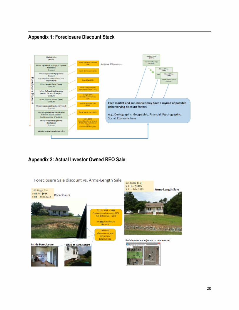
Studies vary widely in the research regarding foreclosure discounting. Recent work by Harding, Rosenblatt and Yao (2012) find the foreclosure discount barely covers the transaction costs of the purchase. They argue that when rehab costs, buyer-barging power, investor or owner-occupant purchaser, neighborhood conditions and demographics are considered, only a small 1.4% per-year discount remains. Pennington-Cross (2006) shows that REO foreclosed properties appreciate less than area-wide appreciation rates due to varying judicial foreclosure laws, loan features and housing market conditions. Other studies report much higher discounts with some averaging 47% or more (Campbell, Giglio & Pathak, 2011). Such dispersion in the findings strengthens the fact that real estate is a heterogeneous asset and prices can reflect varying geographical, economic, legal and demographic attributes within a specific study area. From the researcher’s viewpoint, the discount mechanics are dynamic and can change between market and sub-markets based on a combination of discounting variables. When these variables are added together, they form a discounting mechanism or discount stack unique to each sub-market area of study. Appendix 1 provides a general diagram of the foreclosure discount stack. Data used to conduct the study were obtained from three disparate data sources from County’s tax, geographic (GIS) and Register of Deeds departments and combined into one integrated database. Using a repeat sales panel data methodology, 186 homes were identified as having transitioned through the foreclosure process at four unique periods, including 1.) The arms-length-sale prior to foreclosure; 2.) The foreclosure auction sale; 3.) The REO sale; and finally, 4.) The final arms-length-sale where the property exits the foreclosure cycle. Price changes were recorded for the each transition period, with the average home taking 8.9 years to complete the cycle. Findings show that small scale investors of REO properties had overwhelmingly higher home price appreciation rates than owner occupants during the same period. The findings also show that foreclosures selling out of REO appreciated faster than non-foreclosed properties when compared to the Federal Housing Finance Agency Home Price Index (HPI) (Federal Housing Finance Agency, 2013). These findings have strategic importance for any geographical area experiencing high residential foreclosure rates. First, small scale investors appear more inclined to internalize the costs needed to physically rehabilitate foreclosures and in turn shorten the time such properties stay on the market. Recent studies have found that the length of time a foreclosed property stays on the market, the more negative externality the property has on neighboring home prices (Kobie, 2010). Secondly, the findings show that homes were overpriced at the foreclosure auction and fell an additional 24.13% at the REO sale. In thin-market situations, especially with falling home prices, it may be more prudent to adjust the selling price to appropriately reflect true market valuations. Doing so, shortens the lender’s disposition time and possibly hastens the needed physical rehabilitation of the home. The following sections discuss the overall foreclosure process in North Carolina and the existing literature regarding home foreclosure discounts. Earlier work almost exclusively focuses on the time leading up to the REO sale and the

3    

subsequent impacts foreclosures have on surrounding property values. Although this study follows and measures home price fluctuations throughout foreclosure cycle, the main focus is on post REO home prices and how small scale investors impact the pricing dynamics at this stage of the cycle. Empirical results are given and discussed along with closing conclusions and several policy implications. North Carolina Foreclosure Process The review of literature on foreclosure price discounts centers on two widely debated arguments. First, do actual foreclosure discounts exist after considering a myriad possible economic, financial, demographic, social, spatial, temporal impacts? Secondly, if such a discount does exist, what factors, or combination of factors, contribute to the discount? The literature surrounding this debate is extensive and involves proponents on both sides of the argument; however, recent studies (Frame, 2010) would appear to support the existence of a discount, leaving the second debate, or the amount of discount, open for further scrutiny. The following review describes the residential foreclosure process in North Carolina and distinguishes a foreclosure transaction from a normal arms-length transaction1. Next, a review of existing literature chronicles the ongoing debate surrounding the foreclosure discount and possible explanations for such discounts.

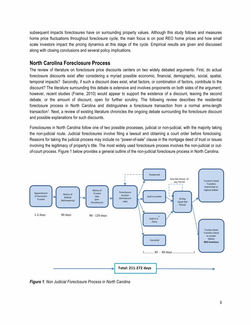
Foreclosures in North Carolina follow one of two possible processes, judicial or non-judicial, with the majority taking the non-judicial route. Judicial foreclosures involve filing a lawsuit and obtaining a court order before foreclosing. Reasons for taking the judicial process may include no “power-of-sale” clause in the mortgage deed of trust or issues involving the legitimacy of property’s title. The most widely used foreclosure process involves the non-judicial or out-of-court process. Figure 1 below provides a general outline of the non-judicial foreclosure process in North Carolina.

Figure 1: Non Judicial Foreclosure Process in North Carolina

Notice  of   Default

(delinquency)

Foreclosure Auction

(foreclosure  sale)

Canceled

Sold  to  3rd

 Party

Sold  to  Lender

Postponed

Notice  of  Trustee Sale (pre-­‐

foreclosure)

Trustee’s  Deed Transfers  

Ownership  to  highest  bidder

Trustee  Deed  Transfers  Deed  

to  Lender  (Bank)

REO  Inventory  

Appointment  of  Successor  Trustee 10  Day  

Upset  Bid  Period

New  Bid  Resets  10  day Period

1-­‐2  days          90  days          90  -­‐  120  days

I………….  30    -­‐    60  days  ……………………….I

Total:  211-­‐272  days

4    

When a mortgage loan is created, a deed of trust is filed in the county where the property is located by the closing attorney. This attorney serves as the trustee in a three-way relationship between the lender and borrower and ensures the agreements stated in the deed are met by both borrower and lender. In most instances, the terms of the deed are honored with the borrower making monthly mortgage payments to the lender. Eventually, the mortgage is paid in full and legal title of the property is transferred to the borrower. While the loan is outstanding, the borrower retains equitable use, possession and enjoyment of the property, but not outright ownership since the mortgage serves as a lien on the property. Only after the loan is satisfied does the borrower own full title to the home. If the borrower fails to make several payments, the power-of-sale clause in the deed of trust allows the lender, through the trustee, to sell the property at public auction. In most instances considerable forbearance measures are exercised by the lender before initiating foreclosure proceedings.

The foreclosure path proceeds sequentially through three stages including pre-foreclosure, foreclosure and post-foreclosure. In the pre-foreclosure stage the lender usually substitutes the original trustee with a firm specializing in foreclosures2. This is done via a written document recorded in the county where the real property resides. Next, a Notice of Default is filed at the courthouse and sent to the borrower, usually by the county sheriff. During this time, called the reinstatement period, the borrower can bring the loan current by making payments in arrears along with any accumulated fees. If the loan is not brought current, the trustee sets a sale date for public auction at the county courthouse on a weekday between 10:00am – 4:00pm. This period is referred to as the Notice of Trustee Sale and advertised publicly at the courthouse and through local newspapers. Even during this period the borrower has a chance to reinstate the loan and pay in full all mortgage payments in arrears, attorney fees and court costs.

The foreclosure stage begins with the trustee sale or foreclosure auction. The sale is conducted and the property sold to the highest bidder. Bidding usually starts with the minimum bid set close to the loan’s current balance. Probable bidders include small LLCs, brokers, contractors and individual investors, or what might be generally considered “mom and pop” investors. For loans with high loan-to-value (LTV) ratios, the home is sold back to the lender and enters into the lender’s Real estate Owned Inventory (REO). At this point the home now belongs to the lender. North Carolina practices a 10-day upset bid period where another party can offer to purchase the property by increasing the reported sales price by 5%. Each time an upset is made, another 10-day upset bid period begins. This process continues until no further bids are made on the property and the last bidder of record becomes the owner. It should be noted that even at this later stage of the foreclosure process, a right of redemption exist and the original owner can regain the home by paying all mortgage payments in arrears, attorney fees and court costs. In total, the pre-foreclosure process to post-foreclosure process can take from 211-270 days. For a detailed discussion of North Carolina foreclosure procedures the reader can refer to Maitin’s (2008) publication for the North Carolina Title and Land Association.

Literature Review Empirical studies attempting to prove or disprove the presence of foreclosures discounts abound in the review of historical literature. The overwhelming conclusion of these studies appears to support a very real discount, with the debate centered primarily on the percentage of the discount. Real estate markets and sub-markets are heterogeneous and it not surprising to find differing empirical results. A majority of the studies use disparate regional datasets; however, several recent studies by the Federal Reserve Bank (Harding, Rosenblatt & Yao, 2012) aggregate multiple regional and metro areas into their models. As real estate researchers well understand, no two locations are exactly homogeneous and finding differing results would not be uncommon.

5    

It is not the intent of this research to further the debate for or against foreclosure discounts, but to simply overview the historical literature surrounding the research. Such research forms the basis for more in-depth and pressing problems such as foreclosure spillover and contagion effects (Gerardi, Rossenblatt, Willen & Yao, 2012) and the many financial and social impacts triggered by foreclosures. This review separates earlier research into several Meta or discounting categories revealed by the literature. Before reviewing these categories however, foreclosure discounts, and more specifically REO foreclosure discounts, are briefly defined.

An REO foreclosure occurs whenever a mortgage servicer, lender, government sponsored enterprise (GSE), Federal Housing Administration (FHA) or Veterans Affairs (VA) entity acquires a home either through voluntary conveyance or after the forced sale at public auction. This repossession process and the eventual resale of the home out of REO create an abnormal or atypical sales process3. Any potential variance in the sales price due to this abnormal process as compared to a normal arms-length sale would constitute a foreclosure discount. Indeed, much of the prior econometric research focuses on proving or disproving the proper controls or attributes to include in the optimal pricing model. As mentioned earlier, determining these unique attributes is difficult due to varying demographic, neighborhood and property characteristics surrounding each home. Foreclosure discounts can be categorized into several functional areas. Independently, each of these factors can contribute to the discount, but more realistically work in combination, forming what might be considered a “discount stack” that represents the aggregate discount similar to that found in Appendix 1. Functional areas highlighted in the research include the condition of the property; general property attributes; market conditions; investment externalities and contagion effects; stigma biases and buyer/seller motivations; liquidity preferences; and regulatory/capital requirements of the seller. Probably the most obvious category includes homes suffering from neglect or deferred operational and capital maintenance (Harding, Miceli & Sirmans, 2000; Summel, 2009; Campbell, Gigilo & Pathak, 2011; Clarretie & Daneshvary, 2009). Such homes tend to be in poorer condition and sell at a lower prices when compared to similar homes. Modeling the appropriate deferred maintenance discount however has been problematic for most econometricians. Placing dollar values on property damage, vacancies and repair costs is not symmetrical across properties and can vary widely by region, neighborhood and property. Likewise, servicers or lenders may rely on broker price opinions (BPO) when establishing REO resale price points. These opinions are often completed through cursory drive-bys of the foreclosed property and may fail to accurately capture deferred maintenance costs. Apgar and Duda (2005) estimated that vacant homes left on the market for extended periods cost municipalities between $5,000 to $35,000 per home depending on the length of vacancy, deferred maintenance and damage. Even if the home were occupied, residents hesitate to maintain a home they foresee as eventually defaulting. Additional studies find that foreclosed properties have common characteristics, such as smaller living spaces, are older, in poorer neighborhoods and have smaller lot sizes (Lee & Immergluck, 2012; Harding & Rosenblatt & Yao, 2012). These findings also highlight one of the more debatable issues surrounding the discount measurement. Opponents contend that abnormal discounts are associated with the characteristics of the home and neighborhood and not simply a reflection of being in foreclosure (Carroll, Clauretie & Neil, 1997; Clauretie & Daneshvary, 2009; Rutherford & Chen, 2012). Empirically, they find that without proper controls for zip codes, neighborhoods, neighborhood foreclosure counts, property condition and size, discounts are probably biased. Likewise, media portrayal and national wide coverage of foreclosures in blighted and vacant neighborhoods such as Detroit creates a stigma or bias toward foreclosures (Cowart & Peng, 2004); however, Pennington-Cross (2006) and Clauretie and

6    

Danshvary find the bias is relatively small when proper controls are included in the model for property condition, location, market impacts. Changing market conditions can also play a significant role in determining the range for foreclosure discounts (Chau & Ng, 2008). Markets such as Phoenix, Arizona; Las Vegas, Nevada; and Miami, Florida are examples where overall market prices, not just foreclosure prices, have experienced wide fluctuations in recent years. Although foreclosures may sell for lower prices, the lower price may simply be a response to overall market price trends (Campbell et al. 2009; Daneshvary, Clauretie, Kader, 2011). Similar to the property condition problem, separating or distinguishing the proper controls for general market movements from those of foreclosures is difficult. Outside of a detailed market appraisal, most datasets used for valuation purposes will inadequately capture rapidly changing price fluctuations and typically lag true market equilibrium prices. A more recent set of studies investigates the investment externality created by foreclosures (Gerardi et al, 2012) and the spillover effects these externalities have on nearby properties (Daneshvary, Clauretie & Kader, 2011; Harding & Rosenblatt & Yao, 2009; Kobie, 2009; Rutherford & Chen, 2012). During the pre-foreclosure and foreclosure process, neither owners nor lenders have an incentive to maintain the property, which over time can lead to deferred maintenance and deferred capital expenditures. From the homeowner’s perspective, this may be attributed to several factors. First, foreclosures are typically triggered when life-changing events occur in the household, such job-loss, death, illness, divorce or some other cash-flow altering event (Campbell et al., 2011). Available cash flowing into the household is used for basic consumption needs creating a disincentive to invest in the property. Secondly, when the owner realizes the home is being foreclosed, there is an added disincentive to invest in the property. Why make repairs when the home is going to be lost anyway. As these deferred maintenance problems persist, neighboring properties eventually succumb to these investment externalities creating a “contagion” of falling home prices throughout the neighborhood (Li, 2013; Gangel, Seiler & Collins, 2013). As more homeowners fall underwater on their mortgages4, more defaults occur creating a feedback loop of falling home prices. In such situations, endogeneity, reverse causality and simultaneity bias becomes more difficult to control (Gerardi, Rossenblatt, Willen & Yao, 2012). Additional costs and disinvestment in the property continues after the home goes into foreclosure. At this point, the lender now owns the property as REO inventory5 and must consume the added expenses in maintaining and selling the property back into the market. Underinvestment can occur since the lender is no longer receiving payments or fees from the defunct mortgage, which is now a non-performing asset on the company’s balance sheet. In many instances the REO agent is merely administering the foreclosure on behalf of a securitized trust and receives no financial benefit from overseeing the property. In such situations, asymmetric information problems can arise between the owner and servicer causing the servicer to ignore possible gains on the resale of the property (Gerardi, et al., 2012). In an effort to minimize the additional holding costs6, servicers may attempt to increase liquidity and reduce the time on the market (TOM) for the property (Jud, Seaks and Winkler, 1996; Taylor, 1999; Clauretie and Thistle, 2007). In summary, the literature overwhelmingly confirms the existence of a foreclosure discount; however, the exact discount amount and proper coefficients to include in any empirical model still appears allusive. This paper argues that no unique model will fully capture each and every foreclosure situation. Markets and sub-markets are compellingly heterogeneous and it is plausible that multiple models will exists to capture the different market variations7. More importantly, the literature reveals the difficulty in controlling for the condition of the property, and to

7    

this point, only superficial attempts to gauge property condition have been attempted8. Gerardi et al. (2012) argue that the most obvious way to deal with such asymmetrical information conditions, where there is no incentive to invest further resources into the property, is to “sell the property to a small-scale investor who internalizes the costs and benefits (p. 21)”. With this statement in mind, we attempt to discover the impact small-scale investors have on market price appreciation rates for foreclosed-residential properties. Data and Methodology

The geographical area of study includes Johnston County, North Carolina, located in the larger Raleigh-Cary metropolitan census area shown in Figure 2. Three separate, disparate databases were used to construct the study’s dataset. Property sales, appraisals and tax records were obtained from the County tax administrator’s office; judicial land records including warranty deeds, deeds of trust and special warranty deeds were obtained from the register of deeds office; and, geospatial and property specific data were obtained from the County’s geographical information systems (GIS) department. Each disparate dataset was integrated into one unique database for analysis purposes9.

Figure 2: Geographical Study Area

Using the integrated data, descriptive statistics were calculated for the county. Instead a point-estimate hedonic approach used in many earlier studies, a panel-data regression methodology was used to capture repeat homes sales transitioning through the foreclosure process. Figure 3 provides a graphical representation of the sales timeline from the first arms-length-sale, trustee sale, REO sale and eventually the final arms-length-sale. In total, four repeat sales were recorded representing the transaction price as the each home moved into and eventually out of foreclosure. In total, 186 single family residential homes were identified as fully completing the cycle. Each home was verified to ensure no major physical changes were made to the home throughout the time period10.

8    

Figure 3. Foreclosure Cycle Timeline

Prior studies (Campbell, Giglio & Pathak, 2011; Sumell, 2009) focus almost exclusively on discovering whether price discounts occur as homes enter into REO status, or from t1-t3. The model created for this study examines the price appreciation occurring from t3 - t4 or when homes eventually transition out of REO status. If a discount does indeed exists, then homes emerging from REO status should produce higher appreciation rates when compared to similar homes in the market. Measuring home price changes with repeat sales provides an alternative to the traditional hedonic approach and uses the price change for houses sold more than once. First introduced by Bailey et al. (1963), the repeat sales approach avoids possible bias estimates for changing home characteristics and quality over time. In this case, the home’s size, location and other distinguishing characteristics are considered time invariant or fixed between transactions. Such time invariant factors can be differenced out between two adjacent selling periods by subtracting home prices at t4 from t3. The price at t3 can be stated as follows:

𝐿𝑛(𝑃!"!) =  𝛽!!! + 𝛽!𝑋!"! + 𝛽!𝑌!"! +  𝛽!𝐺𝑅𝑀!"! +   𝜀!"! (1)

where 𝐿𝑛(𝑃!"!) is the log of the house price i at time t3; 𝑋!"! is a vector of house characteristics for each home i at time t3; Yit3 is a vector of neighborhood or spatial characteristics for house i at time t3; GRM is the gross rent multiplier for house i at time t3; 𝛽!!! is the intercept term and εit is the error term assumed to be independent across observations and identically distributed from a normal distribution with mean zero and constant variance. The GRM variable is added to the traditional hedonic repeat sales method in equation 1 to capture the investor’s view of value at the REO sale. REO purchases by investors, especially distressed REO homes, can represent nearly 60% of REO sales (Brennan, 2012; NAR Investors Survey, 2009). Investors use the GRM measure in gauging the return potential for a specific real estate investment. The calculation is simply the price paid for the home divided by the annual potential rent produced by the home11. Similar to the P/E ratio for stocks, the GRM provides a relative valuation comparison of the home over time. A GRM calculation found in the lower range of its historical average, or that of comparable homes in the area, implies a potentially good investment opportunity. Likewise, homes with higher GRMs may reflect a fully priced home selling at the upper end of its price range with little value-added appeal.

The second equation records the selling price as the home transitions out of foreclosure at t4, or what might be considered the 2nd arms-length-sale in the overall timeline and is specified as follows:

𝐿𝑛(𝑃!"!) = (𝛽!!! +  𝛿!) + 𝛽!𝑋!"! + 𝛽!𝑌!"! + 𝛽!𝐼𝑁𝑉!"!  ) + 𝜀!"! (2)

1st  Arms-­‐Length  

Sale

t1   t4  

Trustee  Sale

 

Home sale Timeline t2  

REO  Sale 2nd    

Arms-­‐Length  Sale

t3  

9    

where Ln(Pit4) is the log of the selling price at t4; (B0t3 + δ) is the intercept plus time dummy representing the intercept at period t4; Xit4 and Yit4 are vectors providing house characteristics and spatial data; and INV is a binary categorical variable capturing whether the home was sold by an owner occupant or investor at t4. Since the Xit and Yit are assumed time invariant and fixed between sales, they can be written as Xi and Yi. Differencing equations 1 and 2 gives the following result:

𝐿𝑛(𝑃!"!) −  𝐿𝑛(𝑃!"!) = [(𝛽!!! +  𝛿!) + 𝛽!𝑋! + 𝛽!𝑌! + 𝛽!𝐼𝑁𝑉!"!  ) + 𝜀!"!] −  [  𝛽!!! + 𝛽!𝑋! + 𝛽!𝑌! +  𝛽!𝐺𝑅𝑀!"! +   𝜀!"!] (3)

And this can be simplified to

𝐿𝑛(𝑃!"!) −  𝐿𝑛(𝑃!"!) =  𝛿! + 𝛽!𝐼𝑁𝑉!"!   −  𝛽!𝐺𝑅𝑀!"! + [𝜀!"! − 𝜀!"!]. (4)

In equation 4 the unobserved effects have been differenced out leaving only GRM and the binary variable Inv. The idiosyncratic error represents the difference between εit4 and εit4. Differencing out the physical and spatial characteristics between the two sales makes logical sense for two reasons. First, a bank, trust or government entity owns the home during the REO period and has no financial incentive to change the home’s current physical design, e.g., room additions, new cabinets, etc. Secondly, neighborhoods typically change over extended periods of time and not in a few months12. The following section provides the empirical results for home sales between the two time periods, along with descriptive results for periods t1-t4, or from the first arms-length-sale until the reemergence from distress at the 2nd-arms-length sale. Empirical Results and Analysis

Ordinary least squares was used to generate the regression results in Table 2 and summary statistics are presented in Table 1. One hundred and eighty six homes were identified as progressing through each of the foreclosure stages from t1-t4. Similar to earlier studies (Campbell, Giglio, Pathak, 2011) foreclosed homes on average sold for less than county wide averages during each period. From 2000-2007 the average home appreciation rate was 29% for all homes sold in the county and from 2000-2012 homes appreciated 18.8% on average. These results reflect general nationwide trends during the same periods. The mean county-wide home price in 2000 was $99,723; by 2007 the average county wide price was $129,074; and, by the first quarter of 2013 the county-wide price had fallen to $115,866.

Homes transitioning into foreclosure, or from t1-t2, experienced a -9.78% drop in median selling price at the trustee auction. The mean time between t1 and t2 was 5.75 years. Homes moving into REO from t2-t3 experienced an additional -25% decline in median price and on average took 203 days to sell. In total, the median home price declined -33.4% (SD=20.5%) from the first arm’s length sale until the REO sale and spanned 8.16 years. The additional drop in median prices from t2-t3, or the difference in prices from the trustee sale to REO sale, represents underwater homes at the trustee sale where the outstanding mortgage balance was higher than the market value for the home, or that lenders were possibly overpricing homes at the auction sale (Fitzpatrick & Whitaker, 2012). During the trustee sale, the lender typically bids an amount equal to the mortgage balance (Bruggerman & Fisher; 2011), even if home’s market value is much less. The data show that homes were falling in price throughout the time period leading up to the REO sale from t1-t3. Similar to the findings of Harding, Rosenblatt & Yao (2012), the dispersion of foreclosure selling prices was wider than normal arm’s length prices during each transition period as noted by the higher standard deviation for foreclosures over normal sales.

10    

Table 1: Summary Statistics

Table 2: Empirical Results

Variable Coefficient Std. Error t-Statistic Prob.

𝛿! .499 .0554 9.43 <.0001*

INV (Binary) .215 .0342 6.31 <.0001*

GRM -.048 .0060 -5.63 <.0001* Note: R2 = .451 F(2, 183) = 75.10 p < .0001*

Dependent Variable: 𝐿𝑛(𝑃!"!) −  𝐿𝑛(𝑃!"!)

Description Variable Mean Median 25% Quartile

75% Quartile

Mean Home Age at Last Sale in years (t4)

Sale Price

1st Arm’s Length Sale (t1) ARM-1 $103,189 $107,000 $91,500 $145,000 Trustee Sale (t2) TR $113,432 $106,000 $83,000 $128,000 REO Sale (t3) REO $84,574 $75,000 $50,000 $105,000 2nd Arm’s Length Sale (t4) ARM-2 $116,586 $113,000 $77,250 $136,625 13 y

Change in Sale Price

Variable Mean Median Std. Dev. Mean Holding Period

(d = days) (y = years)

Arm-1 to Trust (t1-t2) Arm1-TR -9.39% -9.78% 36.4% 5.75 y Trust to REO (t2-t3) TR-REO -24.13% -25.0% 24.28% 230 d Arm-1 to REO (t1-t3) ARM1-REO -34.45% -33.45% 20.57% 8.16 y REO to Arm-2 (t3-t4) REO-ARM2 46.84% 34.83% 40.36% 305 d Arm-1 to Arm-2 (t1-t4) ARM1-ARM2 -5.75% -4.37% 27.7% 8.9 y Home Price Index (HPI) Variable Mean Median Std. Dev. ∆ HPI (t3-t4) HPI-Change -1.16% -.5% 1.8% ∆ HPI to REO-ARM2 (t3-t4) HPI-REO-ARM2 47.9%* 36.85% 40.2% Investor variables Gross Rent Multiplier GRM 6.45 6.65 2.36 Investor Binary Variable INV (Binary)

Change in Price (t3-t4)

Count Mean Median S.D. Mean Holding Period

(d = days) (y = years)

Total Homes 186 (100%) 46.84% 34.83% 40.36% 305 d Owner Bought Homes 52 (27.96%) 13.85% 6.35% 19.07% 1.31 y Investor Bought Homes 134 (72.04%) 56.47% 46.4% 39.64% 254.8 d Note: N = 186 t (183) = 16.06, p < .0001* Avg. Square Footage: 1589

11    

If REO homes are sold at a discount when compared to sales of similar non-foreclosed homes, then the same REO homes sold arms-length at t4 should reveal appreciation rates higher than similar non-foreclosed homes. This assumption is based on numerous studies that show REO sales at t3 sell at discount when compared to arms-length sales. If an arbitrage discount does indeed exist at the REO sale, savvy investors should exploit the price disparity and resell the property at t4 with a sizable gain. To test this assumption each of the 186 foreclosed homes was compared to the county-wide Federal Housing and Finance Agency’s Repeat Sale Home Price Index (HPI) over the same time period. For example, a foreclosed home that sold out of REO inventory on November of 2009 (t3) and eventually resold as an arms-length sale in October, 2010 (t4) was compared to the equivalent county-wide HPI repeat sale index for the same period. The results show that foreclosed homes experienced a 47.9%, t(182) = -11.33, p < .0001, higher mean appreciation rate than HPI index averages during the same period. Again, the variance of foreclosed home appreciation rates was much higher than the HPI index during the period. Median home prices appreciated 36.85% more than equivalent HPI prices, with an average time between sales of only seven months. These findings compare closely with Harding, Rosenblatt & Yao (2012) that show a 33% (SD = 51.83%) excess return for REO homes purchased and then resold within a year. The authors note however that such excess returns were accompanied by much higher risk. As the time between resale increases, excess returns fall, but so does the standard deviation in selling prices. They find that excess returns for homes resold 2-3 years after the REO sale drop to only 4.6% (SD = 13.71%). This study’s findings show similar results, however, prices dropped much more slowly with longer times between resale, with excess appreciation rates dropping by 4.2% for each additional year between t3 and t4. Even with the longer resale period, homes resold 2-3 years after the REO sale had excess appreciation rates of 23.8% (SD = 17.61%). One of the major objectives of the study was to determine the impact investors have on home appreciation rates for homes resold after the REO purchase at t3. Of the 186 homes used in the study, 52 were purchased by owner occupants at the REO sale and 134 were purchased by investors. To determine owner occupants from investors, deeds from the county register’s office were obtained for each of the 186 homes. Homes where the owner’s mailing address was different from the home’s physical address were considered investor owned and homes with identical addresses were considered owner occupied. Owner occupied homes experienced a 6.35% median appreciation in selling price from t3 to t4 with an average holding period of 1.31 years between sales. Investor owned homes experienced a 46.4% median appreciation rate, with a holding period of only 254.8 days. Similar to the comparison with HPI indexes, the higher appreciation rates for investor owned homes were also associated with much higher standard deviations. Using the Satterthwaite Approximation to test the difference between the two means of unequal sample sizes and variances resulted in a significant difference in appreciation rates between investor owned and owner occupant resells, t(146) = -9.66, p < .0001. The short duration in holding period for investor owned homes revealed that many of the homes were bought and resold quickly, or more informally “flipped”. It is interesting to note that REO homes, both investor and owner occupied, saw price appreciations during the t3-t4 period, while the county-wide appreciation rate at all quintiles, as measured by the HPI index, saw price declines during same time period.

To understand the impact investors have on REO home price appreciation rates, the t3 to t4 time period was analyzed through equation 4. Using a log-linear model to control positive skewing of the dependent variable, the equation provided a better overall model fit than a simple linear-linear model. Differencing the two time periods eliminated physical and spatial characteristics from the equation leaving only the INV and GRM variables. As noted earlier, INV is a binary variable that distinguishes investor owned homes from owner occupied homes and GRM is the gross rent multiplier at t3, or when the home was purchased out of REO inventory. Combined, the variables accounted for R2 = 45.1% of the observed variance in home price appreciation from t3-t4, F(2, 183) = 75.10, p < .0001. Interpretation of the log transformed home appreciation rates required transforming unit changes in the predictor parameters to

12    

𝑒!! − 1  𝑥  100 equivalent percentage changes in the dependent variable13. Transforming INV revealed that investor purchased homes at t3 sold for 24.08%, 𝛽! = 𝐼𝑁𝑉 = .2158, t(183) = 6.53, p < .0001, more than owner occupied homes at t4. Transformation of the GRM14 variable revealed that a one unit increase in the gross rent multiplier was associated with a -4.8% change home prices 𝛽! = 𝐺𝑅𝑀 = -.048, t(183) = -5.63, p < .0001. Further comparing the GRM for owner-occupied homes to those of investor owned homes revealed a significant difference in GRM’s between the two groups, t(146) = 4.15, p < .001.

These findings validate the existence of a foreclosure discount, which eventually leads to an above normal appreciation when the foreclosure is resold at arms-length; however, these findings do not include or control for rehabilitation costs of the REO property from t3-t4. Indeed, this single issue underscores the many pro-and-con arguments for or against a discount in the literature and will continue to challenge researchers well into the future (Frame, 2010). We argue that finding such an estimate will always be subjective, and various methodologies are possible. Until recently, prior studies relied on whether the REO property was rated in fair or poor condition (Clauretie & Daneshvary, 2009; Sumell 2009) or possibly vacant when sold (Knight, 2002; Anglin, Rutherford & Springer, 2003; Clauretie & Daneshvary, 2009). To control for rehabilitation expenses, this study uses actual costs from newly formed real estate investment trusts (REIT) buying thousands of foreclosed properties since 2010.

The great rescission of 2008 and the bursting the housing bubble created an abundant supply of foreclosed properties within the United States. To confront the rising supply of foreclosures, the U.S. Department of Housing and Urban Development (HUD) established several REO bulk resale programs to assist in liquidating their supply REO properties (HUD, 2012). At roughly the same time, multiple REITs entered the residential housing and rental market to take advantage of what many, including Warren Buffett, considered a great buying opportunity for homes. Using publically available S-11 registration data from one of these newly formed REITs, American Homes 4 Rent (AMH), actual rehabilitation expenses were extracted from the company’s Securities and Exchange (SEC) filing on 9/13/2013. These costs were documented in the company’s S-11 filing (American Homes 4 Rent, 2013) and contained the following statements:

The acquisition of properties involves expenditures in addition to payment of the purchase price, including payments for acquisition fees, property inspections, closing costs, title insurance, transfer taxes, recording fees, broker commissions, property taxes and homeowner association (“HOA”) fees (when applicable). In addition, we typically incur costs between $5,000 and $20,000 to renovate a home to prepare it for rental. Renovation work varies, but may include paint, flooring, carpeting, cabinetry, appliances, plumbing hardware and other items required to prepare the home for rental. The time and cost involved in accessing our homes and preparing them for rental can significantly impact our financial performance. The time to renovate a newly acquired property can vary significantly among properties for several reasons, including the property’s acquisition channel, the age and condition of the property and whether the property was vacant when acquired. (p. 63).

As of June, 30, 2013, the company had purchased 18,326 single-family homes throughout the United States. Approximately half of these properties were located in the Southeast with an average house age of 11.5 years. Using the S-11 data, median estimates for holding, rehabilitation and selling costs were documented at $13,500 per home. As noted in the S-11 filing, the company purchases 3 to 4 bedroom homes that appeal primarily to upper-end tenants looking for more accommodating and larger homes. This compares closely to the 186 repeat sale homes used for this study, which were 102 square feet smaller and 1.5 years older than the typical AMH home. Converting the

13    

median costs per AMH home to square feet equates to $6.42 per-square foot in additional costs. A percentage of these costs are common for both foreclosure and normal arms-length sales, such as legal, documentation and realtor fees; this implies that the $6.42 number is actually higher than simple repair and rehabilitation expenses alone. For this study, the higher estimate of $6.42 per square foot was added to the price of each home and the empirical results reevaluated.

Including the additional $6.42 in costs to the price of each home at t4, or at the first arms-length sale after REO, resulted in the regression results found in Table 3. Back transforming INV and GRM to their percentage change equivalents revealed at 31.4% higher appreciation rate for investor owned homes at t4 verses owner-occupied homes; and a one unit higher change in the gross rent multiplier resulted in a -2.76% change home appreciation rates. Compared to county returns using the HPI index, a mean difference of 32.88%, t(183) = -12.036, p < .0001, exited between HPI appreciation rates and REO homes being resold at arms-length at t4. Even with the added rehabilitation costs and transaction fees, homes emerging from foreclose appreciated significantly more than similar non-foreclosed homes. Secondly, the findings support the earlier work of Gerardi, et al. (2012) and confirm that investors are willing to internalize the costs needed to eliminate physical deterioration and differed maintenance found with foreclosures in the pursuit of an eventual return on their investment.

Table 3: Empirical Results with Rehab Costs

Variable Coefficient Std. Error t-Statistic Prob.

𝛿! .216 .0659 3.28 <.0001*

INV (Binary) .273 .0407 6.71 <.0001*

GRM -.028 .0072 -3.9 <.0001* Note: R2 = .441 F(2, 183) = 69.60 p < .0001*

Dependent Variable: 𝐿𝑛(𝑃!"!) −  𝐿𝑛(𝑃!"!)

Study Limitations and Future Research

One of the more obvious limitations of the study was limiting it to only one county. As separate governing entities, each county establishes their own processes for implementing state foreclosure laws. For example, Johnston County, the county included in the study, uses separate data repositories for deeds, tax and GIS information; in such instances, aggregating the data was prohibitively time consuming. Add multiple counties, all with differing processes and technologies, and the research effort becomes even more onerous. This apparent opaqueness of foreclosure information may also contribute to the thin market conditions at the trustee auction (Newman, 2010), and thus serves as a further research area.

Many of the homes sold as REO sales were never resold or have yet to transition into an arms-length to arms-length sale at time period t4. Subsequently, as these homes are eventually resold, prices may vary from the results found in the study. The study shows that home price appreciation rates approach normal market rates the longer the home is owned after the REO sale.

14    

Suggestions for future research include conducting the study in differing regional areas to confirm the empirical results. A second suggestion would be to investigate the four panel pricing process during both up and down cycles of the housing market. The t3-t4 period of this study, or the period between the auction sale and REO sale, represented at time of falling home prices. Future research could investigate periods of appreciating home rates and compare them to markets when prices are trending downward, such as Chau and Ng’s (2008) similar work for the Hong Kong market.

Conclusions and Suggestions

This study examined home price appreciation rates for foreclosed residential properties within Johnston County, a county within the Raleigh-Cary Metro area of North Carolina. Using a repeat sales, panel data methodology, 186 homes were tracked over a time period spanning on average 8.9 years per home. The findings show that homes falling into foreclose depreciate in price faster than normal arms-length homes during the same period. Foreclosed homes depreciated in price by 9.78% between the first arms-length sale and auction sale, and dropped another 25% when sold at REO. In total, foreclosed homes lost approximately 34% of their value by the time of the REO sale. Similar results were found by Pennington-Cross (2006) during a period when homes were appreciating in value. His results showed that foreclosed home values appreciated more slowly than average area appreciation rates. The difference in appreciation rates was due primarily to housing conditions, legal constraints and loan considerations. Both studies combined, show that foreclosures appreciate less in up markets and depreciate faster during down markets.

In contrast, homes emerging from foreclosure after being sold out of REO experienced significantly higher price appreciation rates than similar non-foreclosed homes during the same time period. Compared to county returns using the Federal Housing and Finance Agency’s Repeat Sale Home Price Index (HPI) index, homes sold after being purchased from REO appreciated 32.88%, t(183) = -12.036, p < .0001, more than HPI appreciation rates during the same time period. Foreclosed homes completing the foreclosure cycle regained most of their original value with prices mean reverting to comparable arms-length sales within the same area.

Appreciation rates for foreclosed REO homes bought by investors were found to significantly outperform owner occupant homes during the study period. These small scale investors were generally LLCs, real estate brokerages, residential contractors and what many would consider small “mom-and-pop investors”. The findings validate earlier work by Gerardi et al (2012) and show the willingness of investors to take on greater risks in order to eventually resale the property for a profit. Actual repair estimates obtained from a major residential REIT revealed an additional $6.42 per square foot was required to bring a typical foreclosed home up to market-sale conditions. Even when including the extra repair costs, investor-owned REO homes appreciated substantially more than county wide averages for non-foreclosed homes during the same period.

Several commercial and policy-related issues are apparent from the study. First, starting bids for homes sold at the county auction were higher than true market valuations. Fitzpatrick and Whitaker (2012) find that lenders inappropriately value foreclosed homes and overprice homes at the auction sale. The consequences of such overpricing lengthen the amount of time homes languish unsold and further perpetuates a home’s poor physical condition. Instead of setting minimum bids at or near the mortgage balance, lenders should adjust the price to reflect true market-based valuations. Doing so, would incentivize investors to purchase homes during the auction sale, rather than much later at the REO sale. Since investors approach the buying process differently than owner-occupants, appraisers should weight appraisals more heavily towards income valuation methods instead of sales comparison methods. As shown in this study, a simple income-based valuation metric, the gross rent multiplier,

15    

captures relative valuations based on the income potential of each property. Additional income-based metrics, such as capitalization rates and cash-on-cash return to equity could also be advantageous when the buyer pool is more investor centric.

Secondly, these findings support the recent work of Gangel, Seiler and Collins (2013) and show the time a neglected foreclosure lingers on the market impacts neighboring home values more than actual physical externalities. This is important since many of the forbearance and loan modification programs created in the aftermath of the financial crisis, such as the Home Affordable Modification Program or HAMP, were intended to curtail foreclosure rates and stabilize deteriorating home prices. The goal of such programs was to reduce the home owner’s principle mortgage balance thereby lowering the required monthly payments; however, recent reports have revealed such mitigation strategies may have worked to prolong the time many homes languish in pre-foreclosure before succumbing to eventual foreclosure anyway (Sigtarp, 2013). Such programs work in opposition to the findings in this research, which suggest a quicker disposition rather than a longer disposition process may be more beneficial. As this study seems suggest, small scale investors serve a vital role in reducing the time a home remains in foreclosure; these mom-and-pop enterprises accept the risk required to eliminate deferred maintenance found with the home. To that end, their risk-taking efforts contain falling neighborhood home prices, shorten the foreclosure cycle and lessen the impact of negative externalities on adjacent homes.

 

16    

REFERENCES American Homes 4 Rent. (2013). Annual Report. Retrieved October 20, 2013, from

http://investors.ah4r.com/corporateprofile.aspx?iid=4392539 Anglin, M.T., Rutherford, R. and Springer, T.M. (2003). The Trade-off between the selling price of residential

properties and time-on-the-market: The impact of price setting. The Journal of Real Estate Finance and Economics 26, 95–111.

Apgar, W.C.& Duda, M. (2005). Collateral damage. The municipal impart of today’s mortgage foreclosure boom.

Washington, D.C.: Homeownership Preservation Foundation. Retrieved from http://www.995hope.org/wp-content/uploads/2011/07/Apgar_Duda_Study_Short_Version.pdf

Bailey, M. J., Muth, R. & Nourse, H.O. (1963). A Regression method for real estate price index construction.

Journal of the American Statistical Association 4, 933-942. Brennan, M. (2012). Investors Flock to Housing, Looking to Buy Thousands of Homes in Bulk. Forbes, Retrieved

from http://www.forbes.com/sites/morganbrennan/2012/04/03/investors-flock-to-housing-aspiring-to-own- thousands-of-homes/

Bruggerman, W.B., & Fisher, J. ( 2011). Real Estate and Investments. (14 ed.) New York, McGraw Hill/Irwin Campbell, J. Y., Giglio, S. & Pathak, P. (2011). Forced sales and house prices, American Economic Review,

American Economic Association, 101(5), 2108-31. Carroll, T.M., Clauretie, T.M. and Neill, H.R. (1997). Effect of foreclosure status on residential selling price:

Comment. Journal of Real Estate Research, 13, 95–102.

Chau, K.W. & Ng, R. C. K. (2008). Agency theory and foreclosure sales of properties. Journal of Property Science. 1(1), 16-24.

Clauretie, T. M. & Daneshvary, N. (2009. Estimating the house foreclosure discount corrected for spatial price

interdependence and endogeneity of marketing time. Real Estate Economics, 37(1), 43-67.  

Clauretie, T.M. & Thistle, P. (2007). The effect of time-on-market and location on search costs and anchoring: The case of single family properties. The Journal of Real Estate Finance and Economics, 35, 181–196.

Cowart, L. & Peng, C. (2004). Do vacant houses sell for less? Evidence from the Lexington Housing Market. Appraisal Journal 72(3), 234-242.

Daneshvary, N., Clauretie, T. M. & Kader, A. (2011). Short-term own-price and spillover effects of distressed

residential properties: The case of a housing crash. Journal of Real Estate Research, 33(2), 179–208.

17    

Fitzpatrick, T.J., Whitaker, S. (2012). Overvaluing residential properties and the growing glut of REO. Federal Reserve Bank of Cleveland, Economic Commentary, Retrieved from http://www.clevelandfed.org/research/commentary/2012/2012-03.cfm

Federal Housing Finance Agency. (2013). Home Price Index Data. Retrieved June, 5, 2013 from the Federal

Housing Finance Agency Website: http://www.fhfa.gov/Default.aspx?Page=87 Forgey, F.A., Rutherford, R.C. & VanBuskirk, M.L. (1994). Effect of foreclosure status on residential selling price.

Journal of Real Estate Research 9, 313–318. Frame, W. S. (2010). Estimating the effect of mortgage foreclosures on nearby property values:

A critical review of the literature. Federal Reserve Bank of Atlanta Economic Review, 95(3), 1-9. Gangel, M., Seiler, M. J. & Collins, A. J. (2013). Exploring the foreclosure contagion effect using agent-based

modeling. Journal of Real Estate Finance and Economics, 46(2), 339-354. Gerardi, K., Rossenblatt, E., Willen, P.S. & Yao, V.W. (2012). Foreclosure externalities: Some new evidence,

Working Paper 2012-11. Federal Reserve Bank of Atlanta, Ga. Retrieved from http://www.frbatlanta.org/documents/pubs/wp/wp1211.pdf.

Harding, J. P., Rosenblatt, E. & Yao, V.W. (2009). The contagion effect of foreclosed properties. Journal

of Urban Economics, 66, 164–178. Harding, J P., Rosenblatt, E., &, Yao V. W. (2012). The foreclosure discount: Myth or reality? Journal of Urban

Economics, 71(2), 204–218. Hardin,W.G. & Wolverton, M.L. (1996). The relationship between foreclosure status and apartment price. Journal

of Real Estate Research, 12, 101–109. Harding, J., Miceli, T.J. and Sirmans, C.F. (2000). Do owners take better care of their housing than renters?

Real Estate Economics, 28, 663-681. Jud, G.D., Seaks, T.G. & Winkler, D.T. (1996). Time-on-the-market: The Impact of residential brokerage. Journal of

Real Estate Research 12, 447–458. Knight, J.R. (2002). Listing price, time on market, and ultimate selling price: Causes and effects of listing price

changes. Real Estate Economics, 30, 213–237. Kobie, T. (2010). Residential Foreclosures' Impact on Nearby Single-Family Residential Properties: A New Approach

to the Spatial and Temporal Dimensions. (Electronic Thesis or Dissertation). Retrieved from https://etd.ohiolink.edu/

Lee, Y. S. & Immergluck, D. (2012). Explaining the pace of foreclosed home sales during the US foreclosure

crisis: Evidence from Atlanta. Housing Studies. 27(8), 1100-1123.

18    

Li., L. (2013, April). Why are foreclosures Contagious? Paper presented at the 2013 FSU-UF Critical Issues in Real Estate Symposium Housing Market Issues: Initiatives, Policies and the Economy. Abstract retrieved from http://www.fsurealestate.com/downloads/5_FSU-UF%20Why%20Are%20Foreclosure%20Contagious%20- %20Li.pdf  

Maitin, L.S., (2008) Real property foreclosure procedures. The North Carolina Land Title Association. Retrieved

from http://www.maitinlaw.com/wp-content/uploads/2013/07/NCLT-Real-Property-Foreclosure-Procedures.pdf

National Association of Realtors. (2009). NAR Investors Survey. Washington, DC: National Association of Realtors. Newman, K. (2010). Using publically available data to understand the foreclosure crisis. Journal of the American

Planning Association, 76 (2), 160-171. Pennington-Cross, A. (2006). The value of foreclosed property. Journal of Real Estate Research, 28, 193–214.

Rutherford, R., & Chen, J. (2012).  Foreclosure, quality and spillover in residential markets. International Journal of

Housing Markets and Analysis, 5(1), 53-70. Shilling, J.D., Benjamin, J.D., & Sirmans, C.F. (1990). Estimating net realizable value for distressed real estate.

Journal of Real Estate Research, 5, 129–139. Springer, T.M. (1996). Single family housing transactions: Seller motivations, price, and marketing time. The Journal

of Real Estate Finance and Economics, 13, 237–254. Sumell, A. (2009). The determinants of foreclosed property values: Evidence from inner-city Cleveland.

Journal of Housing Research, 18(1), 45–61. Taylor, C.R. (1999). Time-on-market as a sign of quality. Review of Economic Studies, 66, 555–578 The Office of the Special Inspector General for the Troubled Asset Relief Program (SIGTARP). (2013). Quarterly

Report to Congress, July 24, 2013. Retrieved from: http://www.sigtarp.gov/Quarterly%20Reports/July_24_2013_Report_to_Congress.pdf.

U.S. Department of Housing and Urban Development. (2012). Retrieved August 25, 2013, from

http://portal.hud.gov/hudportal/HUD?src=/program_offices/housing/comp/asset/sfam/sfls Zillow. (2013). Zillow Home Rent Locator. Retrieved from: http://www.zillow.com/homes/johnston-county-nc_rb/ on

July 7, 2013.

19    

Endnotes                                                                                                                          1  The  foreclosure  process  described  refers  only  to  the  state  of  North  Carolina  and  predominately  the  Trustee  Sale  Process.    2  In  North  Carolina  such  firms  as  Brock  and  Scott  PLLC;  Shapiro  and  Ingle  PLLC;  Rogers,  Townsend  &  Thomas  PC  and  Hutchins  and  Sentor  PLLC  make  a  market  in  handling  foreclosures.    3  Normal  homes  sales  are  typically  transacted  by  owner  occupants  selling  to  other  potential  owner  occupants.    4  An  underwater  homeowner  is  when  the  home  owner’s  house  value  is  worth  less  than  the  outstanding  mortgage  on  the  home,  or  when  the  loan-­‐to-­‐value  (LTV)  is  greater  than  one.  Although  most  home  owners  never  succumb  to  foreclosure  when  underwater,  the  number  of  foreclosures  generally  increases  when  homeowners  owe  more  on  the  mortgage  than  the  home  is  worth.      5  The  asset  moves  from  the  non-­‐performing  loan  pool  to  the  OREO  or  REO  physical  asset  pool  on  the  balance  sheet.    6  Holding  cost  can  include  insurance,  maintenance  costs,  taxes,  time-­‐value  of  money  holding  costs,  brokerage  fees  and  attorney  fees.      7  Indeed,  private  companies  now  create  automated  valuation  models  (AVM)  that  can  be  cascaded  to  capture  unique  valuation  differences  for  specific  market  or  demographic  situations.        8  Note  however  that  these  attempts  exclude  a  full  property  appraisal  where  a  human  actually  goes  inside  the  property.    9  Support  for  this  study  would  not  have  been  possible  without  the  effort  of  GIS  and  tax  administrators  from  Johnston  County  geographical  mapping  and  tax  departments.    10  Physical  changes  include  items  that  would  have  changed  the  assessed  value  of  the  home,  such  as  added  square  feet,  remodeled  rooms,  garage  additions,  etc.    New  county-­‐wide  appraisals  were  conducted  near  the  end  of  the  study,  so  comparisons  were  made  of  pre  and  post  appraisals  to  find  any  changes.  Homes  that  could  not  be  verified  by  record,  thirty  six  homes  in  total,  were  physically  inspected,  either  by  contacting  the  owner  or  visiting  the  location  to  ensure  no  physical  changes  had  occurred  during  the  study  period.  11  Rent  rates  were  obtained  from  Zillow.com,  which  supplies  rental  estimates  at  the  neighborhood  level.    12  The  average  days  on  market  (DOM)  for  an  REO  in  North  Carolina  is  approximately  250  days.    13  To  interpret  dependent  log  transformed  variables,  the  predictor  coefficients  must  be  back  transformed  to  interpret  the  original  percentage  change  format.  This  is  usually  done  by  exponentiation  of  the  coefficient  using 𝑒!! − 1  𝑥  100,  or  approximately  100b1.  14  Gross  Rent  Multiplier  uses  the  annual  rent  divided  by  the  price  of  the  home  to  determine  a  yield  value  for  the  property.  Rent  area  data  was  obtained  from  Zillow.com,  which  carries  rent  data  for  the  house,  community  and  neighborhood.                                      

20    

                                                                                                                                                                                                                                                                                                                                                                                                       Appendix 1: Foreclosure Discount Stack

Appendix 2: Actual Investor Owned REO Sale