A COMPARISION OF TRADITIONAL AND ACTIVE LEARNING …

A COMPARISION OF TRADITIONAL AND ACTIVE LEARNING METHODS:

AN EMPIRICAL INVESTIGATION UTILIZING A LINEAR MIXED MODEL

by

DAVID WELTMAN

Presented to the Faculty of the Graduate School of

The University of Texas at Arlington in Partial Fulfillment

of the Requirements

for the Degree of

DOCTOR OF PHILOSOPHY

THE UNIVERSITY OF TEXAS AT ARLINGTON

December 2007

iii

ACKNOWLEDGEMENTS

It is difficult to explain the work that is involved in conceiving an idea,

conducting an experiment, collecting data, performing a literature review, deciding how

to analyze the data in a reasonable manner, and writing dissertation text. It genuinely

takes a community of experts who are willing to sacrifice valuable time for this

contribution. My committee members were always very welcoming, open, and

generous with their time. Members provided expertise at different points in the

dissertation process. Some provided a great deal of help in the beginning, some more in

the analysis phase, but all were active with advice, time, and reference materials over

the past year and a half. I would like thank Dr. Whiteside for agreeing to supervise my

dissertation and keeping me on track. I had no idea of the efforts involved in being a

supervising professor, and I greatly thank Dr. Whiteside for taking on this responsibility

and welcoming it. Thanks to Dr. Eakin for providing direction, suggestions, and

reference materials early in the process. Without Dr. Eakin’s thoughts and

recommendations early in the idea development, my dissertation certainly would not

have content as rich as I hope it now has. Also, thanks to Dr. Eakin for carefully

correcting some of my experimental materials and providing student perspectives on the

experiment. Thanks to Dr. Hawkins, for unbelievable generosity of time and mixed

model expertise. Over the past year, Dr. Hawkins always welcomed me into his office,

sometimes multiple times per day. Thanks to Dr. Grisaffe for his thoughtful

iv

suggestions, recommendations, and inspirational support. Dr. Grisaffe also provided a

number of thoughts as to future research with this topic. His advice will definitely help

me become a better scholar in the future. It does take courage, tenacity, and diligence

to take on a project of this nature. I also want to thank Dr. Nancy Rowe, our University

statistician. Dr. Rowe provided a great deal of help with SPSS, and I now have so much

more expertise with statistical analysis software thanks to her. I also greatly appreciate

the support and help from our department. Andrea Webb has been a friend, guide, and

source of support throughout this process.

November 14, 2007

v

ABSTRACT

A COMPARISION OF TRADITIONAL AND ACTIVE LEARNING METHODS:

AN EMPIRICAL INVESTIGATION UTILIZING A LINEAR MIXED MODEL

Publication No. ______

David Weltman, PhD.

The University of Texas at Arlington, 2007

Supervising Professor: Mary Whiteside

This research aims to understand what types of learners (business school

students) benefit most and what type of learners may not benefit at all from active

learning methods. It is hypothesized that different types of students will achieve

different levels of proficiency based on the teaching method. Several types of student

characteristics are analyzed: grade point average, learning style, age, gender, and

ethnicity.

Three topics (in the introductory business statistics course) and five instructors

covering seven class sections are used with three different experimental teaching

methods. Method topic combinations are randomly assigned to class sections so that

each student in every class section is exposed to all three experimental teaching

vi

methods. A linear mixed model is utilized in the analysis. The effect of method on

student score was not consistent across grade point averages. Performance of students

at three different grade point average levels (high, middle, low) tended to converge

around the overall mean when learning was obtained in an active learning environment.

Student performance was significantly higher in a traditional method (versus an active

learning method) of teaching for students with high and mid-level grade point averages.

The effects of the teaching method on score did not depend on other student

characteristics analyzed (i.e. gender, learning style or ethnicity).

vii

TABLE OF CONTENTS

ACKNOWLEDGEMENTS....................................................................................... iii ABSTRACT .............................................................................................................. v LIST OF ILLUSTRATIONS..................................................................................... x LIST OF TABLES..................................................................................................... xi Chapter Page 1. INTRODUCTION………. ............................................................................ 1 2. LITERATURE REVIEW.............................................................................. 6 2.1 Background………….............................................................................. 6 2.1.1 Bloom’s Taxonomy of Cognitive Domain ............................... 9 2.1.2 Learning Styles ......................................................................... 11 2.2 Themes in Active Learning Research…………...................................... 13 2.2.1 Frameworks .............................................................................. 13 2.2.2 Games…….. ............................................................................. 15 2.2.3 Use of Technology.................................................................... 18 2.2.4 Cooperation…........................................................................... 19 2.2.5 Active Learning Controversy….. ............................................. 22 3. RESEARCH METHODOLOGY ............................................................. 24 3.1 Background………………...................................................................... 24

viii

3.1.1 Description of the Topics.......................................................... 25 3.1.2 Description of the (3) Teaching Methods................................. 26 3.1.3 Description of the Assessment.................................................. 28 3.2 The Base Research Model ....................................................................... 29 3.3 Research Questions….............................................................................. 30 3.4 Experimental Approach ........................................................................... 31 3.5 Data Collection…….. .............................................................................. 33 3.6 Research Design…….. ............................................................................ 33 3.7 Hypothesis Tests…….............................................................................. 35 3.8 Ordinary Least Squares and Generalized Least Squares Using Maximum Likelihood Estimation…….. ....................................... 44 3.9 Randomization to Sections Versus Individuals…….. ............................. 45 3.10 Handling of Missing Data…….............................................................. 50 4. ANALYSIS OF RESULTS........................................................................... 53 4.1 Demographic and Descriptive Data......................................................... 53 4.2 Research Question 1 - Main Teaching Effects ........................................ 58 4.3 Research Questions 2, 3, and 4 – Interaction of Gender by Method, Learning Style by Method, and Ethnicity by Method ............... 59 4.4 Research Questions 5 and 7 – Interaction of Grade Point Average by Method….............................................................................. 61 4.5 Research Question 6 – Significance of the Random Effects ................... 69 5. CONCLUSION………….. ........................................................................... 71 5.1 Discussion……………............................................................................ 71 5.2 Future Auxiliary Analysis…………….................................................... 76

ix

5.2.1 Bloom’s Taxonomy and Higher Levels of Learning................ 76 5.2.2 Instructor Method Effectiveness............................................... 77 5.2.3 Inclusion of an Order Indicator Variable.................................. 77 5.2.4 Consideration of One Comprehensive Model .......................... 77 5.3 Implications in Research.......................................................................... 78 Appendix A. SPSS CODE .............................................................................................. 82 B. SPSS OUTPUT – CUSTOM CONTRASTS ............................................. 90 C. INFORMED CONSENT ........................................................................... 94 D. QUIZZES UTILIZED IN ASSESSMENT ................................................ 98 E. END OF SEMESTER STUDENT SURVEY ............................................ 106 F. SPSS OUTPUT – ALL MODEL RUNS .................................................... 108 REFERENCES .......................................................................................................... 117 BIBLIOGRAPHY...................................................................................................... 122

x

LIST OF ILLUSTRATIONS

Figure Page 1.1 Bloom’s Taxonomy of Cognitive Domain...................................................... 9 3.1 Bloom Assessment Plot................................................................................... 28 3.2 An SPSS Student Data Record........................................................................ 33 4.1 Model Adjusted Means Plot, Spring 2007 Data.............................................. 64 4.2 Model Adjusted Means Plot, Summer 2007 Data........................................... 68

xi

LIST OF TABLES

Table Page 3.1 Random assignment of methods to class sections........................................... 34 3.2 Mean Adjusted Model Example...................................................................... 36 4.1 Description of Study Variables ....................................................................... 54 4.2 Overall Descriptive Statistics .......................................................................... 56 4.3 Demographic Statistics.................................................................................... 57 4.4 Main Effect Hypothesis Test Results .............................................................. 58 4.5 Method by Gender, Learning Style, and Ethnicity Interactions...................... 59 4.6 Tests of Fixed Effects in the Gender Inclusive Model.................................... 60 4.7 Tests of Fixed Effects in the Learning Style Inclusive Model........................ 61 4.8 Tests of Fixed Effects in the Ethnicity Inclusive Model................................. 61 4.9 Method by Grade Point Interaction for Each Model....................................... 61 4.10 Testing Method by GPA Interaction ............................................................... 63 4.11 Parameter Estimates in the Final Model ......................................................... 63 4.12 Point Estimates for Three GPA Levels in Each Method (spring 2007) .......... 64 4.13 Confidence Intervals of Mean Differences in Methods for Three GPA Categories with a Family Confidence Coefficient of .95 ............ 66 4.14 Confidence Intervals of Mean Differences in Methods for Three GPA Categories with a Family Confidence Coefficient of .90 ............ 66

xii

4.15 Point Estimates for Three GPA Levels in Each Method (summer 2007) ....... 68 4.16 Results of Tests for Random Effects............................................................... 70 5.1 Results of Hypothesis Tests ............................................................................ 75

1

CHAPTER 1

INTRODUCTION

Universities and business schools provide many important functions in our

society. These functions include knowledge transfer, community involvement, and

scholarly research among other things. Certainly, an important function of the

university is teaching students, expanding their knowledge, and enhancing their lives

through learning. This idea is articulated in the 2006-2010 strategic plan

(http://activelearning.uta.edu) for The University of Texas at Arlington which gives as

its top goals/priorities:

Planning Priority I: “Provide a high quality educational environment that

contributes to student academic achievement, timely graduation and preparation to meet

career goals,”

Goal 2: “Increase the effectiveness of the learning process.”

The McCombs School of Business at The University of Texas in Austin also

echoes the importance of effective teaching in their mission statement

(http://www.mccombs.utexas.edu/about/mission.asp) which states:

“The mission of the McCombs School of Business is to educate the business

leaders of tomorrow while creating knowledge that has a critical significance for

industry and society. Through innovative curriculum, excellent teaching, cutting-edge

research, and involvement with industry, the school will bring together the highest

2

quality faculty and students to provide the best educational programs and graduates of

any public business school.”

The first statement of overview at the Harvard Business School

(http://www.hbs.edu), arguably the best business school worldwide (http://grad-

schools.usnews.rankingsandreviews.com), states: “The mission of Harvard Business

School is to educate leaders who make a difference in the world.” Thus, it is clearly an

important priority for business school educators to provide an excellent educational

environment. New learning tools and techniques, such as active or experiential

learning, that have the potential to enhance an educational environment are of particular

interest to business school researchers (Anselmi & Frankel, 2004; Barak, Lipson, &

Lerman, 2006; Hansen, 2006; Raelin & Coghlan, 2006; Yolanda & Catherine, 2004).

Although action learning as a concept dates back centuries, in modern times, it was first

described in detail by the English scholar R.W. Revans (1971) who further developed

the concept over the following two decades. Briefly, Revans refers to action learning as

reflection on experience and states that learning is achieved through focusing on

problems in a social context (Revans, 1983), i.e. managers learning from each other and

enhancing learning through interaction and shared experiences. More recently, Bonwell

and Eison (1991) define active learning as “instructional activities involving students in

doing things and thinking about what they are doing.” The concept of active learning

has evolved over time, and this evolution is further described in section 2.1.

Several studies (Raelin & Coghlan, 2006; Sarason & Banbury, 2004; Sutherland

& Bonwell, 1996; Ueltschy, 2001; Umble & Umble, 2004) have demonstrated both

3

quantitative and anecdotal evidence regarding the effectiveness of active learning

techniques. This research develops further understanding of active learning effects by

empirically analyzing data obtained by conducting a semester long experiment in a

quantitative business school course (undergraduate business statistics). More than 300

students agreed to participate in the experiment, which was formally approved by The

University’s department on human research. The experiment involved seven class

sections and five business school instructors. Subject characteristics such as gender,

ethnicity, learning style, and grade point average were used to determine which

characteristics were important in estimating how well a student performs under a

particular teaching method. All students received each of the three teaching methods.

The treatments were randomized to class section. Thus, some students received

instruction in a topic under a certain teaching method, whereas, other students received

instruction in the same topic under a different teaching method. The binomial

distribution topic was administered to groups of students in the three different teaching

methods, depending on class section, as were the other two topics (sampling

distributions and p-values).

Prior to commencement of the experiment, it was assumed that the effects of

topic and class section would be important. These effects are controlled for by treating

them as random effects in all hypotheses tests. All estimates are adjusted based on the

class section and topic involved. Important learner characteristics are analyzed to

understand what groups may benefit most and what groups may not benefit at all from

active learning environments. Various learner characteristics in this study include;

4

gender, learning style, ethnicity, and cumulative grade point average. Three levels of

learning are utilized (traditional, semi-active, and fully-active) and subjects’ are then

tested on various levels of learning outcomes. Using Bloom’s taxonomy of cognitive

domain (Bloom, 1956) as guide for question development, students are assessed

immediately after a learning session to measure the effectiveness of the technique on

the subject. In future research, student preference for each type of learning method may

also be measured to determine if other potential moderating effects exist.

The traditional classroom lecture has been the dominant teaching method in

business schools today, as well as in the past (Alsop, 2006; Becker, 1997; Brown &

Guilding, 1993). “In relatively few instances in established business schools is there

much clinical training or learning by doing—experiential learning where concrete

experience is the basis for observation and reflection” (Pfeffer & Fong, 2002). Current

assessments of this technique show potential for improvement to this long-standing

tradition (Bonwell, 1997). There is increasing competition among business schools,

student expectations about teaching are rising, and students are seeking an active, high-

impact learning experience in the classroom (Auster & Wylie, 2006). Furthermore,

business students are demanding more engaging learning experiences that are worth the

opportunity of putting their careers on hold or adding additional burden to already busy

lives (O'Brien & Hart, 1999; Page & Mukherjee, 2000; Schneider, 2001).

This dissertation reviews some of the numerous studies providing justification

that there are benefits in using active learning methods. Overall, students appear to

favor this method of learning over the more traditional methods although a significant

5

amount of the business research in active learning is anecdotal in nature. This

dissertation also reviews some of the controversy in active learning. Our research

suggests that in a quantitative undergraduate business course where students have

limited background understanding, active learning methods may not be effective at all

and in fact may degrade the learning of higher-level students. This research provides

specific empirical evidence regarding the effectiveness of such new experiences.

Important student characteristics are compared to determine whether or not differences

in learning achieved for a particular method are significant based on these

characteristics.

The effects of active learning on undergraduate business students are analyzed,

and a statistical model is developed to study such effects. The research provides an

empirical analysis based on a number of important student characteristics in the domain

of active learning to determine which characteristics play a role in the effectiveness of a

particular teaching method. In the present study, cumulative grade point average was

important in determining the effectiveness of a teaching method. Performance of

students with a high grade point average level significantly degraded when exposed to a

highly active learning method as compared to a traditional teaching method.

Performance of students at a low grade point average level increased although this

improvement is not deemed significant. This research in business training potentially

adds to further refinement in the ongoing development of newer learning systems in an

increasingly competitive and student needs-oriented university environment.

6

CHAPTER 2

LITERATURE REVIEW

2.1 Background

Ideas about active learning are very longstanding, as shown by several ancient

Chinese proverbs about experiential learning which are commonly cited. Some are

attributable to the philosopher Lao-Tse (5th century B.C.), who is alleged to have said:

“If you tell me, I will listen. If you show me, I will see. But if you let me

experience, I will learn.”

Another example of the long history of active learning comes from Benjamin

Franklin who wrote, “Tell me, and I may forget. Teach me, and I may remember.

Involve me, and I will learn.” These thoughts have withstood the test of time and are

testimony to the potential of learning through active involvement.

More recent ideas about active learning can be traced to the great and influential

American philosopher John Dewey (1859 -1952), who wrote extensively about

education and the benefits of learning through practical experience. Certainly many of

active learning’s tenants likely have origins in the philosophy of Dewey’s pragmatism.

Dewey and other philosophers (C.S. Peirce, 1839-1914 and William James, 1842-1910)

active in the late 19th century espoused that “models of explanation should be practical,

in accord with scientific practices.” If a theory could not be proven through scientific

principals and experimentation, it would not be seriously regarded. It is easy to link

7

these ideas to education and training where pragmatists could only believe that hands-

on, experiential learning were the best methods of instilling knowledge. No doubt,

Dewey held little regard for learning through passive listening and rote memorization of

facts. Stemming from this philosophy of pragmatism, Dewey believed that only

through practical experience, i.e. learning by doing, could students broaden their

intellect and develop important problem solving and critical thinking skills.

The term “active learning” was introduced by the English scholar R.W. Revans

(1907-2003) who was quite instrumental in promoting this type of educational method

across the world. Charles Bonwell and James Eison, scholars in teaching excellence,

are recognized in their more recent promotion of effective active learning techniques.

There is no single, definitive definition of active learning. A clarification of the

term comes from Bonwell (1991) where he states that in active learning, students

participate in the process and students participate when they are doing something

besides passively listening. Active learning involves engagement with the material

being learned (Stark, 2006). Active learning is something that “involves students in

doing things and thinking about what they are doing” (Bonwell & Eison, 1991). Action

learning is highly reflective (Davey, Powell, Powell, & Cooper, 2002). Keeping the

ideas of these scholars in mind, perhaps active learning is really best thought of as a

“student-involved learning continuum.” At the low end of the spectrum there must be

some involvement other than simply listening; at the extreme end of the spectrum,

students are fully engaged in the learning process, exploring and applying ideas on their

own. At this high end of the active learning continuum, it is posited that greatest

8

learning benefits can be achieved. It is believed that in this setting students will be able

to achieve the highest levels of learning - that is, they are able to synthesize and

evaluate (Bloom, 1956). Thus, active learning is thought of as a method of learning in

which students are actively or experientially involved in the learning process and where

there are different levels of active learning, depending on student involvement.

The idea of active learning for the purpose of this research is to think of it as a

broad category of experiential techniques that can vary in intensity or level across a

continuum. A high-intensity active learning technique would be one in which students

are highly involved in a learning experience such as using the principals of project

management to build a catapult and then using the principals of statistics in

summarizing results of accuracy in launches. Highly active learning techniques could

involve the participation in a simulation such as the MIT beer game

(http://beergame.mit.edu), where students compete to manage a supply chain process.

A less-involved experiential learning experience might entail watching a video, then

breaking into teams to perform a workshop, and then applying what was learned from

watching the video. Even lower-level forms of active learning may simply involve

pauses in a traditional lecture to allow students time to think about or discuss the

concepts presented.

The concept of active learning is fairly open-ended and evolving. With the

continual advent of new technologies, there are many possibilities that can enhance

student experiences. Maybe most importantly, active learning provides opportunities

9

for unique and innovative student experiences. Using active learning ideas, instructors

can create unconventional, creative, and fun learning environments.

2.1.1 Bloom’s Taxonomy of Cognitive Domain

A classic and popular reference model that can be used to analyze and study the

effectiveness of various teaching methods is Bloom’s Taxonomy of the Cognitive

Domain (Bloom, 1956). Bloom’s taxonomy was chosen as a tool for this study to help

develop and assess student learning outcomes following a teaching method. This model

was chosen for a variety of reasons. Bloom’s model is well established and remains a

very popular tool for development and assessment of teaching and training tools,

especially in educational environments, which is the context for this study. Application

of the taxonomy is relatively simple and clear. The framework is hierarchal so that

basic knowledge is assessed at the lowest level and more complex learning can be

assessed at the highest levels. Bloom’s taxonomy of cognitive domain is summarized in

Figure 1.1 below.

Figure 1.1: Bloom’s Taxonomy of Cognitive Domain

At the low end of the hierarchy is Knowledge. Students with knowledge level

skills are able memorize and regurgitate ideas and principals. A business statistics

Synthesis Evaluation

Analysis

Application

Comprehension

Knowledge

Synthesis Evaluation

Analysis

Application

Comprehension

Knowledge

10

student with knowledge skills would be able to recognize the central limit theorem, for

example. Comprehension is the next level in the hierarchy. Students with

comprehension level understanding are able to describe, summarize, and translate.

Here, a student is able to explain the central limit theorem to another student, for

example. In application level knowledge, students are able to apply a concept to a

familiar problem. With this level of knowledge, students are able to properly utilize the

central limit theorem in a particular type of situation. An example would be using the

standard normal table to determine the probability that the mean of a sample falls in a

certain range of values when a sample, of say thirty five, is selected. With analysis,

students have the ability to not only apply but also to classify, compare, and contrast.

Here, students are able to understand when it would be appropriate to apply the central

limit theorem and be able to explain why. A student would be able to provide an

alternate tool to solve a problem and explain why the alternate tool is more appropriate

for the issue at hand. Synthesis and Evaluation are at the highest level of the Bloom

taxonomy. Students with synthesis and evaluation skills invent, create, judge, and

critique. Here students can create “add on” ideas to concepts to solve new problems.

Original thought occurs. Clearly, these skills are the most difficult and complex to

develop. It has been posited that active learning environments facilitate the

development of these higher-level skills (Paul & Mukhopadhyay, 2004).

The assessment and development of the three training methods in this research

are consistent with the Bloom taxonomy. The development of training materials gives

students the opportunity to learn across much of the Bloom spectrum from simple facts

11

and ideas about the concept being taught, to being able to analyze a new situation and

possibly invent a solution that was not previously discussed. The assessment used in

this research tests the students on their mastery of knowledge, capability to apply

knowledge, and ability to determine the applicability of learned solutions to new

situations. The construction of the training and assessment materials were developed

utilizing Bloom’s framework as an important and critical guide.

2.1.2 Learning Styles

The concept of learning styles has origins in Carl Jung’s personality types.

Jung’s four basic personality types are broken into two categories. The first category

has to do with decision making, and the second category concerns how we gather

information. Thinking and feeling are two ways in which people make decisions. No

one exclusively makes decisions by either method, but Jung posited that in most people

one characteristic is dominant. Thinkers tend to use logic, thought, and extensive

analysis in decision making, whereas feelers base decisions or make judgments on a

“gut feel.” Feeling-based decisions are subjective, thinking-based decisions are

objective. The second category has to do with how we perceive and gather information.

Again, Jung derived two ideas, one of which is dominant, but not exclusively used in

most people. According to Jung, people gather and perceive information through

sensation and intuition. As the name suggests, sensation is sensible, practical, and

realistic. Sensation-dominant people gather information in a methodical manner by

using senses such as aural or visual. Intuition-dominant people, on the other hand, learn

more through pictures, concepts, and imagining things. Intuition-dominant people tend

12

to learn best through understanding the “big picture” and have less regard for details

and facts. Jung’s four basic personality types are currently very well accepted and have

been used as the basis in the development of numerous personality type, social

interaction, and learning measures. Using Jung’s seminal ideas as a backdrop and

further educational research (Dunn, 1983; H. Reinhardt, 1976) involving perceptual

learning channels, Fleming and Mills (1992) developed the VARK (Visual, Aural,

Read/write, and Kinesthetic) learning style assessment tools, which are the learning

preferences utilized in this research. VARK was selected for a number of reasons.

VARK is consistent with major, significant learning research. VARK is practical, easy

to use, and easy to understand. Students are able to go to a website (www.vark-

learn.com), answer a 16-question survey, and obtain their learning preferences. By

using the VARK, students have a further advantage of being able to view study

suggestions based on their learning preference. These recommendations can

significantly enhance a student’s educational experience. In the VARK classification

system, visual learners are individuals who prefer graphs and symbols for representing

information. Aural learners learn best by listening and would likely enjoy lectures.

Read/write learners prefer the written word and may learn best through reading

materials. Finally, kinesthetic learners prefer a hands-on approach to learning. This

research empirically tests the relationship between learning style and teaching method.

It is thought that students with different learning preferences, as measured using the

VARK questionnaire, will have achieved differing topic skill levels depending on the

teaching method utilized.

13

2.2 Themes in Active Learning Research

In reviewing literature in active learning in business research, five overall

themes appear to be important in this domain: frameworks, games, use of technology,

cooperation, and controversy. The subsequent sections provide an overview sample of

some of the research in these areas.

2.2.1 Frameworks

The framework research articles reviewed tend to be conceptual in nature and

have to do with ideas for creating effective environments, assessment, and preparation

for active learning in the classroom. Auster and Wylie (2006) discuss four dimensions

of the teaching process that create active learning in the business classroom. These

dimensions are: context setting, class preparation, class delivery, and continuous

improvement. Context setting has to do with establishing a climate and setting norms

that will facilitate more student involvement. Making students feel comfortable asking

questions and being actively involved are part of creating a context setting that is

appropriate for learning. Auster and Wylie argue that it is important to establish this

type of environment early in a classroom. Getting to know students and setting

expectations are part of creating an effective context setting. The other three

dimensions are more directly focused on the teaching process. Most instructors focus

on effectively preparing topic content. In Auster and Wylie’s four-dimensional model,

there is a focus on both content and delivery of the content. Careful preparation of how

content is delivered is integral to effective experiential learning. Many of Auster and

Wylie’s classroom techniques are consistent with those of other active learning

14

scholars’. The ideas emphasize end of session takeaways, thought/reflection time, and

utilization of a variety of teaching modes including: debates, discussion of relevant

current events, and games.

Bonwell (1997) discusses a framework for the introduction of active learning

with a special focus on assessment. It is important to actively assess knowledge in the

class by checking the class during a lecture using short questions such as, “Did

everyone get that?” Questions can be displayed giving students the opportunity to think

about them before the answer is illustrated for the entire class. Practice quizzes and

peer assessment ideas are discussed as ways to actively assess knowledge and help

demonstrate important lecture topics to students. Bonwell also emphasizes the

importance of group participation (cooperation discussed in section 2.2.4) and explains

techniques for facilitating active learning using such groups.

Hillmer (1996) introduces a problem-solving framework utilized for teaching

business statistics to MBA students. Hillmer argues that statistics has become more

relevant for potential business managers over time, and that the best way to emphasize

its relevance is through application. The best way to design a quantitative course for

business students is to center it around problem solving. Hillmer goes on to argue that

“most students are interested in learning things that they will be able to apply,” and thus

a course design needs to teach students in a context. A key idea in the Hillmer

framework is that instead of trying to find places for a tool, such as regression analysis,

students should focus on a thorough understanding of the problem and then pick the

appropriate statistical analysis technique. One of the problems with this structure is that

15

students need a good understanding of the basic statistical techniques available and of

how to apply them. In an introductory statistics course, achieving such a high level of

comprehension is often not possible, especially in the first half of the course. Still,

Hillmer’s ideas of context and “real-world” application of course design have many

merits that could certainly be utilized to enhance a business student’s education.

2.2.2 Games

The use of games as a method of content delivery is a popular technique in

active learning in business schools. This popularity stems from several factors:

enjoyment, stimulation of competitive spirit, and a natural affinity towards games.

Games are frameworks students seem to easily relate to.

Oftentimes in business statistics, the accurate mathematical results obtained

from applying correct analysis and method is counterintuitive to the student. A

common example that has been studied is the Monte Hall problem (Umble & Umble,

2004). In this problem, a contestant is given three doors from which to choose. Behind

one of the doors is a new car, behind the other two doors are goats. Obviously, the goal

is to select the door with the car. After the contestant selects a door, the host (who

knows which door the car is behind) opens a door with a goat behind it. The contestant

is then asked if she would like to switch her choice. Statistically, the contestant should

switch as her odds improve from one-third to a two-thirds chance of winning.

Typically, students believe that it makes no difference, switching or staying and it is

difficult to convince students otherwise through traditional lecture approaches, using

decision trees for example. However, when students use a hands-on approach and

16

simulate the game multiple times, they become believers and have a better

understanding of the statistical theory. Umble and Umble conclude that using the

experiential, hands-on approach is more effective than the lecture approach in achieving

desired learning outcomes with respect to the teaching of this concept in probability.

Results from the Umble and Umble study are based on a questionnaire in which

students self-report their learning and interest in the exercise.

Reinhardt and Cook (2006) have developed extensive semi-active learning

materials for conducting review sessions for undergraduate and graduate operations

management courses at DePaul University. The material is inspired by the Who Wants

to be a Millionaire® television show and is available for educational purposes at

http://candor.depaul.edu/~greinhar/wwtbam.html. In these sessions, students simulate

the Millionaire game complemented with instructor explanations and clarifications.

Students take a more hands-on approach to learning through playing the game to review

operations management concepts. Aspects of active learning are clearly involved in this

project in that there is more student participation and opportunity for reflection than in a

traditional lecture review format. The researchers found that a large majority (77%) of

the students enjoyed and felt that game was beneficial in helping them understand and

review operations management concepts. There was a high success rate (92%) for

(regurgitation, repeat) questions involving Bloom’s knowledge level of understanding.

It was not specified what the success rates were for questions involving higher levels of

the cognitive domain.

17

Roth (2005) describes the use of a highly active learning workshop in which

LEGO® bricks are used to teach students difficult cost accounting concepts. In this

workshop, students are part of a manufacturing process in which various departmental

costs are derived. The workshop gives students the opportunity to learn cost accounting

principals as well as to apply this knowledge in initiating cost reduction processes. The

workshop is also used as basis for foundation knowledge for a future topic (quality and

supply chain management). Based on student self-reported scores, Roth found the

utilization of the workshop to be effective in increasing student understanding of the

cost accounting concepts and to be an effective use of class time.

The use of television game show formats has been suggested as a means of

incorporating active learning into the business classroom. Sarason and Banbury (2004)

suggest that popular game shows such as Who Wants to be a Millionaire or Jeopardy

are “common experiences” for many students, and by using these formats as classroom

lesson “frames,” students become more engaged in learning. Many instructors accept

the premise that active learning is beneficial for enhancement of student knowledge, but

there are few techniques that are relatively easy to incorporate into business lesson

plans. The use of popular television game shows can be a fairly easy and effective

method of providing students with active learning experiences. Sarason and Banbury

further suggest that through the use of these ideas, students achieve higher levels of

learning.

18

2.2.3 Use of Technology

A number of scholars have performed studies involving the use of technology to

promote active learning. It is believed that in this age of technology, constant

communication, and interactivity that students will come to expect more technologically

enhanced environments (Li, Greenberg, & Nicholls, 2007). Furthermore, some

researchers believe that such tools will be needed in order to maintain student interest

and motivation (Ueltschy, 2001). Examples of this type of research vary widely.

Simple use of technology involves the use of personal computer software tools such as

statistical software packages that allow students to develop histograms or utilize applets

that generate sampling distributions. Other examples involve the use of networked

computers to allow student collaboration online to solve more complex problems. For

example, researchers (Barak, Lipson, & Lerman, 2006) implemented wireless laptop

computers to understand how live demonstrations and a computerized, hands-on

approach would aid students in learning introductory information systems and

programming concepts. Results showed that the use of technology increased student

enjoyment and interaction, but was also a source of distraction and was commonly used

for “non-learning purposes.”

Paul and Mukhopadhyay (2001) implemented technology in a study of sixty-

five graduate students enrolled in two sections of an international business course. A

software program was set up to facilitate student collaboration through the use of e-

mail, discussion groups, and chat rooms. Students with the enhanced technology tools

were compared to a control group. Results showed that collaboration and access to

19

information was enhanced, but contrary to expectations, the use of this technology did

not significantly improve students’ analytical and problem solving abilities. Paul and

Mukhopadhyay’s exploratory research could not find much conclusive evidence about

the use of technology to develop high-level synthesis and evaluation skills, but some

anecdotal evidence was found to suggest that information technology can be utilized to

improve some higher-level student skills such as critical thinking and creativity.

Li and Nicholls (2007) implemented sophisticated software to allow a class to

get involved in a virtual business to better understand the ramifications of various

product marketing choices. In this virtual business simulation, MBA students spent up

to 20 hours per week establishing businesses and making various marketing decisions.

Collaboration with other business managers (classmates) was integral to the tool.

Results showed that students enjoyed the experience, became involved, and felt as

though the simulation was a good surrogate for real-world experience. But, similar to

other research reviewed, this study did not empirically test students on the knowledge or

skills achieved. The researchers only asked the students how they felt about knowledge

gained in a number of areas related to product marketing. Students rated the “good use

of class time” category less than other items assessed; however, the overall ranking was

preferred to the traditional lecture-centered method.

2.2.4 Cooperation

An important part of active learning is working and discussing situations with

peers. An instructor may tell students how to solve a particular problem, but oftentimes

learning occurs when students discuss problem-solving techniques with each other.

20

Revans (1971) suggested that reflection is an important part of the learning process.

Other researchers (Mumford, 1993; Pell, 2001; Vince & Martin, 1993) extend this

concept by suggesting that business managers learn by reflection with other managers

as they focus and work through real world business issues. Mumford and Honey

(1992), for example, stressed that “learning is a social process in which individuals

learn from and with each other.” Most business managers look for employees with

social skills who can work collaboratively in teams to solve problems (Garfield, 1993).

Active learning using cooperative approaches is well suited for preparing business

students because of its social, teamwork, and real-world applicability (Sims, 2006). As

reviewed, there seems to be clear justification for utilizing collaboration and teamwork

in the business classroom. Garfield (1993) goes on to point out several ways in which

students benefit through classroom cooperation: explaining a concept to someone else

improves understanding, students motivate and encourage each other, differing/alternate

solutions to problems can be compared and discussed, shy students may more easily ask

a question to a peer, and working with other students may create a positive feeling.

Laverie (2006) emphasizes the importance of team-based active learning as an

approach to effective development of marketing skills. This research posits that,

through the use of team-based exercises, students will develop a deeper understanding

of course material. Furthermore, this approach will improve students’ readiness for

working in a complex business environment. An exploratory, three-level methodology

is utilized, all involving small teams. First, recent articles or current events are used to

challenge the teams to apply marketing concepts in a problem solving approach.

21

Second, during lectures, a student response system is utilized to keep students involved

during class and to immediately assess understanding. The student response system is

also an example of using technology to facilitate active learning, discussed in the prior

section. Third, case studies are employed to “pull together and further apply

information to solve problems.” Consistent with other studies reviewed, students found

the teamwork-based activities to be valuable and enjoyable. Student self-reported

results indicated a positive feeling about learning and understanding course material.

Students also strongly felt that the activities would help them develop skills needed in

the workplace.

Cooperative methods are not without issues. Kvam (2000) noticed that one

problem is that when such methods are over-utilized, more talented students become

tired and grow frustrated with less-talented teammates. Another challenge of

cooperative approaches is the efficient use of class time. This researcher has

consistently implemented a cooperative workshop approach to demonstrate the effect of

sample size on p-values in hypothesis testing. Anecdotal evidence indicates that

students enjoy this activity, but clearly some time is not effectively used and overall, the

workshop approach takes about twice as long to cover the same material as in a more

traditional approach. Kvam also noticed an increase in time taken to cover a particular

topic as well as increased preparation time.

22

2.2.5 Active learning controversy

Active learning is intuitively appealing and fun for students. Instead of listening

to a “boring” lecture, students get to collaborate and participate in learning exercises.

Depending on the setting, there may also be a sense of excitement in the classroom, if a

role play or debate is about to commence. As cited in the following sections, there is a

significant amount of anecdotal and some empirical evidence as to the overall benefits

of active learning. To be fair, there is also evidence that experiential learning is less

effective and less efficient than more direct approaches (Kirschner, Sweller, & Clark,

2006; Klahr & Nigam, 2004; Mayer, 2004; Sweller, 2003). This may be especially true

for less experienced learners with little prior knowledge (Kirschner, Sweller, & Clark,

2006). It makes intuitive sense that these types of learners need a more guided and

structured approach to achieve mastery of a particular topic. There are several other

challenges involved in the implementation of active learning teaching methods. To my

knowledge, there is no established model or paradigm for utilization of this method,

especially in business school courses. Thus, teachers utilizing active learning

techniques are really pioneers that are experimenting with approaches that may or may

not be effective. There are not many examples to follow nor is there an abundance of

supporting materials available. These issues can create additional instructor workloads.

Based on this researcher’s experience, it may be more difficult for students to gain

potential benefits from active learning in large class sections. Students need instructor

support and guidance when taking on more responsibility and becoming more involved

in the learning process. With large class sections taught by one instructor, there is less

23

time available for instructor expertise. Instructors are well aware that oftentimes

increased “face time” leads to higher levels of learning. Finally, it is quite unclear what

type of students may benefit from active learning. Certainly, different cultures or social

upbringing make a difference in how students learn. A student from a certain type of

background may be very bright but exceptionally shy. If this type of student were thrust

into an in-class role play or debate, he might be so uncomfortable that any content could

not be assimilated. Similarly, it is possible that gender or past academic achievement

might play a role in affinity towards a particular style of teaching and learning. Thus,

this research seeks to begin a process of sorting out which type of students learn the

most, and which type of students benefit least, from different types of teaching methods

based on a simple three-level active learning continuum.

24

CHAPTER 3

RESEARCH METHODOLOGY

3.1 Background

In this study, an experiment was conducted to determine the effects of different

levels of active learning on business students with differing demographic, background,

and learning characteristics. More than 300 students in 7 sections of undergraduate

business statistics participated in the semester-long experiment. A linear mixed model

was chosen for analysis since study factors have both fixed and random effects. The

effect of a factor is said to be fixed if the factor levels have been specifically selected by

the experimenter, and if the experimenter is interested in comparing the effects on the

response variable of these specific effects (Dean & Voss, 1999). Such is the case with

our teaching methods, and thus, this factor is treated as fixed. When a factor has a large

number of possible levels, and the levels included in the experiment are a random

sample from the population of all possible levels, the effect of the factor is said to be

random (Dean & Voss, 1999). Levels of a random effects factor are not of particular

interest to the experimenter. We are interested in studying the effects of various

teaching methods regardless of effects that may be because of the particular instructor

or topic. Thus, section, topic, and subject effects are treated as random effects factors in

this experiment. Since this experiment involves factors with both fixed and random

effects, a mixed model is used. Variability in random effects factors is controlled for in

25

a mixed effects model. This variability may occur as students in an experienced

instructor’s class may score higher overall than in a less experienced instructor’s

section, for example. Similarly, some topics are harder to master than other topics, and

thus, students would be expected to score lower in these more difficult topics, all else

being equal. This research is not primarily concerned with this type of variability. The

treatment of these factors as random factors control for any such natural variations that

may occur.

This research is concerned with the effects of the teaching methods utilized on

various types of students. The mixed models implemented control for variation that is

not of primary interest in this project (random subject, topic, and section).

3.1.1 Description of the Topics

Based on the experience of the researcher and suggestions from committee

members, three topics were chosen for the experiment. Every effort was made to select

topics that covered a fairly wide range in level of difficulty, but leaning toward more

difficult topics. The rationale behind trying to select topics that were more difficult is

that a greater range of quiz score results would be obtained. In general, we sought

topics that were complex enough to challenge all types of students so that we could

obtain a range of rich and varied outcomes. The three topics chosen were the binomial

distribution, sampling distributions, and the concept and calculation of p-values in

hypothesis testing. In the binomial distribution content, students are taught the basic

ideas that underlie the distribution, where its application is appropriate, assumptions,

and basic calculations of binomial probabilities for various scenarios. The mean,

26

variance, and skewing causes are also covered in this topic. In the second topic,

students learn the basic ideas of sampling distributions. The central limit theorem and

the concept of standard error are covered. In the p-value approach to hypothesis testing,

students are exposed to the idea of a test statistic under conditions where the population

standard deviation is both known and unknown. Various hypothesis testing scenarios

are covered and techniques for calculating p-values are explained by using tables (the

standard normal and student t) and Microsoft Excel.

3.1.2 Description of the (3) Teaching Methods

This research uses three teaching methods: a “traditional” lecture, an enhanced

lecture, and a workshop. A teaching method is administered in a fifty to sixty minute

session where a particular experimental topic is covered. The traditional lecture

teaching method is likely the most widely used technique in business schools today. In

this teaching method, students sit and listen to a lecture that has been structured and

prepared by the instructor. This method is often supplemented with Microsoft Power

Point slides and class notes.

Sutherland and Bonwell (1996) suggest that incorporating short experiential

learning activities into a traditional lecture may be an effective way to gain many of the

benefits of active learning with a minimum amount of disruption to the familiar lecture.

In this research, I refer to this environment as the semi-active or enhanced lecture

method. Effective strategies for a semi-active or enhanced lecture method include: the

pause procedure, short writes, and think-pair-share (Bonwell & Sutherland, 1996).

These authors argue that after about 15 minutes of lecture, students’ ability to assimilate

27

material rapidly declines. The pause procedure allows students to take a short break to

compare notes and get mentally refreshed for a couple of minutes before the lecture

continues. Short writes involve asking students to periodically take 3 to 5 minutes to

summarize main points presented. In Think-Pair-Share, students are periodically asked

questions from the lecture and to discuss potential answers with peers. Results are then

shared with the entire class in a discussion format. All these semi-active techniques get

students involved to an extent and break up a potentially long lecture. The ideas of

getting students involved in a penalty-free environment are central tenants of the semi-

active method. This research implements the semi-active method through the use of the

traditional method punctuated with several breaks for students to collaborate on

questions posed by the instructor. These lecture pauses focus on applications of and

computations based on statistical methods. For example, after about 15 minutes of

lecture regarding the binomial distribution, students are asked to come up with example

situations where application of the binomial distribution would be appropriate. After

another approximately 15 minutes of lecture, students are asked to calculate simple

binomial probabilities that were discussed.

A collaborative workshop has the highest level of student involvement of the

three teaching methods. In the workshop, students may work in small teams (i.e. two or

three students) utilizing documentation that has been developed by the researcher.

Here, the instructor works more as a “consultant” than a lecturer. Students are

responsible for their own learning but have an expert available to answer questions and

provide guidance concerning a particular topic.

28

3.1.3 Description of the Assessment

A 15-20 minute multiple-choice quiz follows an experimental session. Subject

performance is measured by the percent of questions answered correctly. The

underlying strategy for question development and student assessment in this experiment

is Bloom’s taxonomy of cognitive domain. Questions were designed to assess a fairly

wide variety of skills obtained. Questions were also designed to test relatively simple

skills, such as the ability to recall and define, as well as much more complex skills, such

as the ability to compare, apply, and utilize techniques appropriately. Overall, the

majority of questions fall into the Bloom taxonomy of comprehension, application, and

analysis, with a few questions assessing higher and lower levels of learning. Figure 3.1

below shows the entire set of questions plotted on the Bloom continuum.

Figure 3.1: Bloom Assessment Plot

Knowledge

Comprehension

Application

Analysis

Synthesis

Evaluation

B1 B2

B3 B4 B5

B6

B7

B8

S1

S2 S4 S5

S3 S6

S7

P1

P2 P3

P5

P4P6

Knowledge

Comprehension

Application

Analysis

Synthesis

Evaluation

B1 B2

B3 B4 B5

B6

B7

B8

S1

S2 S4 S5

S3 S6

S7

P1

P2 P3

P5

P4P6

Knowledge

Comprehension

Application

Analysis

Synthesis

Evaluation

KnowledgeKnowledge

ComprehensionComprehension

ApplicationApplication

AnalysisAnalysis

Synthesis

Evaluation

Synthesis

Evaluation

B1 B2B1 B2

B3 B4 B5B3 B4 B5

B6

B7

B8

S1

S2 S4 S5S2 S4 S5

S3 S6S3 S6

S7

P1

P2 P3

P5

P4P6

29

3.2 The Base Research Model

A primary goal of model selection is to choose the simplest model that

provides the best fit to the observed data (West, Welch, & Galecki, 2007). This idea of

parsimony is echoed throughout many statistical writings. Section 4, analysis, provides

details about the model fitting procedures utilized. For discussion purposes, the

following simple model is proposed:

atoropic indict is the t

catorethod indim is the m

, indicatorsectionj is the

dicator, subject inisiwhere

TCSxxY ijmttjjiijmt

,

)( )( εβ ++++=

ijmtY is the subject’s test score (response) measured as percent correct for subject

(or student) i nested in section j, method m, and topic t. Each subject is tested a total of

three times, and thus, there are three repeated Y measurements for each student. ijmtε is

the associated random error term. The first term, βx , represents fixed effects, with the

remaining terms, ijmttjji TCS ε+++)( , representing the random effects in the model.

mµ (not shown but implicit in the model above) represents the overall mean for a

particular teaching method. x is a vector that represents student characteristics of

interest: gender, ethnicity, grade point average, and learning style. The three test scores

for each subject are possibly correlated as the stronger students may have higher scores

than weaker students. A high score in one method-topic combination might well be

associated with high scores in the other two method-topic combinations. The proposed

30

mixed model accounts for these possible correlations. Implicit in the fixed effects

section of the model are interactions. Interactions between method and important

student characteristics (gender, learning style, GPA, ethnicity) are considered.

This study considers subject/student, section, and topic as random effects. We

consider each of these factors as random selections from a large population of

possibilities. S is the variable for the random subject factor, C is the variable for the

random section factor, and T is the variable for the random topic factor. Possible

variation in scores due to subject, section, and topic are not of primary interest in this

study. For example, the three topics used in the study come from a large population of

possible topics and are selected only as a matter of convenience, not because of any

particular study interest in those topics. The mixed model adjusts for possible variation

in these random effects.

3.3 Research Questions

1. For three study models (gender inclusive, learning style inclusive, and

ethnicity inclusive), are there significant differences in student learning due to three

experimental teaching methods while controlling for any potential effects due to class

section, topic, and cumulative grade point average?

2. For a gender inclusive study model, are there differences in the effects of

teaching methods on learning depending on the gender (or sex) of student, while

controlling for cumulative grade point average, class section, and topic?

31

3. For a learning style inclusive study model, are there differences in the

effects of teaching methods on learning depending on the learning style of student,

while controlling for cumulative grade point average, class section, and topic?

4. For an ethnicity inclusive study model, are there differences in the

effects of teaching methods on learning depending on student ethnicity, while

controlling for cumulative grade point average, class section, and topic?

5. Are there differences in the effects of teaching methods on learning

depending on a student’s grade point average, while controlling for class section and

topic?

6. Are the estimates of random effects for class section and topic

significant?

7. For any significant differences found in research questions 1 through 5,

what is the size (or importance) of these differences? What are reasonable upper and

lower limits for these differences?

Research question 1 is addressed in hypotheses 3.1.2, 3.2.2, and 3.3.2. Research

questions 2, 3, and 4 are addressed in hypotheses 3.1.1, 3.2.1, and 3.3.1. Research

question 5 is addressed in hypotheses 3.1.3, 3.2.3, and 3.3.3. Research question 6 is

addressed in hypotheses 3.4.1 and 3.4.2.

3.4 Experimental Approach

In an effort to address the proposed research questions, an experiment involving

more than 300 undergraduate business students was developed and performed. It was

desired to study the effect of three different teaching methods on different types of

32

subjects. The first method is the traditional lecture method, and the other two methods

are differing levels of active learning. The second teaching method, referred to as the

semi-active level or method, involves the use of traditional lecture techniques, but with

short activity breaks every 10-15 minutes. In these short breaks, students are given an

exercise that may be performed with a classmate. This activity gives students a chance

to reflect on the material that has been presented and to demonstrate his or her

knowledge. Student collaboration, often integral to active learning, may occur in this

method. The third method, referred to as the fully-active level, involves a workshop.

Students work in pairs using computers and materials developed for self-study and

reflection about a particular topic. In this method, the instructor acts primarily as a

consultant when questions arise. Here, students have the least amount of structure or

guidance, but work with materials and technology intended to engage them in a

particular topic.

Three experimental learning sessions were held over the course of a semester.

Each student is exposed to each of the three methods. Following a session, the student

takes a short multiple-choice test to assess his or her mastery of the topic. Questions

were developed to assess learning using various levels of Bloom’s taxonomy of

cognitive domain. Low-level questions involving simple memorization and

regurgitation as well as high-level questions involving the application of concepts and

selecting appropriate techniques are also assessed.

33

3.5 Data Collection

Data for this experiment is collected from three sources. First, there are three

repeat measurements for each student. The source of these measurements is test scores

(percent correct) from the three experimental class sessions. Second, demographic data

is collected from student registrar records. Third, a survey is administered to obtain

learning style data and other demographic data not available from the registrar. Figure

3.2 shown below illustrates all the data collected for each experimental subject.

Figure 3.2: An SPSS Student Data Record

3.6 Research Design

In each of seven sections of the undergraduate business statistics course, three

80-minute class sessions are involved in the experiment. In an experimental class

session, an instructor teaches a topic using the teaching method and materials specified

Student Identifier Number

Section

Topic 1 Score

Topic 1 Method

Topic 2 Score

Topic 2 Method

Topic 3 Score

Topic 3 Method

SAT Score, Math and Verbal

Age

Gender

Ethnicity

GPA

Classification

Major

Self-reported study habits

Self-reported attendance

Self-reported work hours

Learning Style

Registrar

Self-report/survey

Quiz

Student Identifier Number

Section

Topic 1 Score

Topic 1 Method

Topic 2 Score

Topic 2 Method

Topic 3 Score

Topic 3 Method

SAT Score, Math and Verbal

Age

Gender

Ethnicity

GPA

Classification

Major

Self-reported study habits

Self-reported attendance

Self-reported work hours

Learning Style

Registrar

Self-report/survey

Quiz

34

and developed by the researcher. Following an experimental session, students take a

short (15-minute) multiple-choice test (Appendix D).

Seven different class sections and five different instructors were involved in this

experiment. Each instructor was randomly assigned a method sequence for three topics.

Table 3.1 shown below, shows the method sequence for the seven Spring 2007 class

sections (the capital letters refer to instructors). Instructors D and E have two sections

while instructors A, B, and C have one.

Table 3.1: Random assignment of methods to class sections

Per a standard course syllabus, the topics are covered sequentially in time as

listed in Table 3.1. The binomial distribution topic is covered first, followed by

sampling distributions later in the semester. Finally, the p-value topic in hypothesis

testing is covered near the end of the semester. There are several beneficial aspects of

this design. Every instructor teaches each topic, and each topic is taught using each

method. Thus, every student is exposed to all three methods. The methods are

sequenced three different ways. Instructors A and B are using method 1 first, method 3

second, and method 2 last. Instructors C and D are using method 3 first, method 2

EA,BC,D3-PValues

A,BC,DE2-Sampl Dist

C,DEA,B1-Bin Dist

3-Full Act2-Semi Act1-Trad

To

pic

Method

EA,BC,D3-PValues

A,BC,DE2-Sampl Dist

C,DEA,B1-Bin Dist

3-Full Act2-Semi Act1-Trad

To

pic

Method

35

second, and method 1 last. Instructor E is using method 2 first, method 1 second, and

method 3 last. The same assessment test is implemented for each topic, regardless of

the teaching method used.

Data for the experiment is collected from several sources. Test scores are

obtained after the instructor has completed a session and administered the test. Certain

student demographic data is obtained from the university registrar office. Other student

data such as study, habits, work hours, and attendance are self-reported. Data about

student learning style is collected from the VARK questionnaire website analysis

(www.vark-learn.com). Approximately 25 data points were collected for each of the

300 students involved in this research, the most important being the test scores (our

response variable) for each of the three methods.

3.7 Hypothesis tests

The main question that this research addresses regards the interaction of the

methods with student characteristics. For example, we wish to know whether any

differences across methods are consistent across gender. This research seeks to

understand whether any differences across methods are consistent across learning style

as well as ethnicity. We seek to understand if there are differences in the effects of the

three teaching methods on learning depending on the subject’s grade point average.

These questions are answered with hypothesis tests involving the interaction terms.

Main effects for the teaching methods are also tested for three study models. We test

whether or not there are significant effects in student learning because of teaching

method, while controlling for any potential random effects of class section and topic.

36

The following section provides a general explanation of how hypothesis tests

are performed while controlling for a covariate. In the example that follows, we are

interested in determining whether any differences in methods are consistent across

gender, while controlling for a continuous fixed factor, grade point average, in this

example. A continuous adjustment strategy with the technique of covariate centering is

used. An abbreviated study model is shown below:

average point grade target a is T and

T - GPAA (i.e. centered is whichvariable average point grade the is A

Female), if 0 Male,if 1(G variable indicator gender the is G

3, Methodif 0 M2and 13 M

2, Methodif 0 M3and 1M2

1, Methodif 0M3M2

method level reference the is 1 Method where

AMAMAGMGMGMMScore

0

0 ),

382763524332210

=

=

==

==

==

+++++++++= εβββββββββ

Table 3.2 shows how the model represents mean scores adjusted to a particular

target grade point average, :),()( 0 0mg TA m, MethodgGenderYET ====µ

Table 3.2: Mean Adjusted Model Example

Method Gender )( 0Tmgµ Model Representation

1 1 )( 011 Tµ 30 ββ +

1 2 )( 012 Tµ 0β

2 1 )( 021 Tµ 4310 ββββ +++

2 2 )( 022 Tµ 10 ββ +

3 1 )( 031 Tµ 5320 ββββ +++

3 2 )( 032 Tµ 20 ββ +

37

The hypothesis of whether or not, controlling A=T0, there is a gender method

interaction is,

.0:

:

)()()()()()(:

54

53433

0320310220210120110

==

+=+=

−=−=−

ββ

βββββ

µµµµµµ

0

0

H

to reduces which

H

testing to equivalent is which

TTTTTTH

Similarly, to test other hypotheses of interest, the same technique is utilized. To

test whether or not there is a significant ethnicity X method interaction, the incremental

value of the terms related to ethnicity by method terms are tested. To test whether or

not there is a significant learning style X method interaction, the incremental value of

the terms related to learning style by method terms are tested and so on. To test

whether or not there is a significant cumulative grade point average X method

interaction, the significance of the interaction term is tested.

Likelihood ratio tests (LRTs) are utilized to test the significance of the fixed-

effect parameters. The LRTs for the fixed main effects are based on maximum

likelihood (ML) estimation (Casella & Berger, 2002; Morrell, Pearson, & Brant, 1997;

Pinheiro & Bates, 2000; Verbeke & Molenberghs, 1997; West, Welch, & Galecki,

2007). We utilize these methods to test the significance of the main effects. LRT’s

compare the relative likelihoods (of data) under null and alternative hypothesis.

Lambda (λ) represents this likelihood ratio of null to alternate hypothesis. A large

lambda value is indicative of results being more likely to occur under the null

hypothesis, whereas relatively small lambda values are indicative of the results being

38

more likely to occur under the alternate hypothesis. A -2 log-likelihood (-2LL) of the

lambda value under each hypothesis is compared, i.e. subtracted from each other. This

test statistic is then compared to the familiar chi-squared distribution, which is a

reasonable approximation of the null distribution of the -2LL distribution for large

sample sizes. Alternately, some researchers (Fai & Cornelius, 1996; Verbeke &

Molenberghs, 1997) recommend for the present mixed model application of an

approximate Type III F-test using the Satterthwaite method (and restricted maximum

likelihood estimation) for obtaining approximate degrees of freedom to test these main

fixed effects. Approximate Type III F-tests (as opposed to Type I F-tests) are utilized

since they are conditional on the effects of all terms (fixed and random) in a given

model versus only the fixed effects in a Type I F-test (West, Welch, & Galecki, 2007).

Both methods (likelihood ratio tests based on ML estimation and approximate F-tests)

are implemented (in section 4) for hypothesis tests involving main fixed-effect

parameters. Both methods are utilized to check for consistency in any conclusions and

inferences that are made.

To test for significance of the method by student characteristic interaction, a

Type III F-test is utilized. For example, to obtain the test statistic for testing whether

the gender X method interaction is significant, a Type III F-test is used with

Satterthwaite approximated degrees of freedom. This technique is described in detail

by West, Welch, and Galecki (2007).

39

Research question 6 regarding the significance of random effects Cj and Tt are

tested using hypotheses related to the variance of the class section and topic effects as

follows:

0:

0:

0:

0:

2

(

2

(0

2

(

2

(0

>

=

>

=

)topict1

)topict

section)classj1

section)classj

H

H

and

H

H

σ

σ

σ

σ

To test these hypotheses, a likelihood ratio test is utilized which compares the –2 log-

likelihood value for a reference model to a –2 log-likelihood value for a model which

omits the random class section or random topic effect. The asymptotic null distribution

of the test statistic is a mixture of 2χ distributions, with 0 and 1 degrees of freedom,

and equal weights of .5 (Verbeke & Molenberghs, 1997; West, Welch, & Galecki,

2007). Restricted or residual maximum likelihood estimation (REML) introduced by

Patterson and Thompson (1971) is the method proposed for estimating variance

components and testing the random effects since our study involves an unbalanced

design. REML is preferred to ML estimation for testing random effects, because it

produces unbiased estimates of covariance parameters by taking into account the loss of

degrees of freedom that result from estimating the fixed effects in β (West, Welch, &

Galecki, 2007). If the difference in the two models (full versus reduced) is represented

by the symbol d, then the p-value for the likelihood ratio test statistic is:

)(5.0)(5.0 2

1

2

0 dPdPvaluep >∗+>∗=− χχ (3.4.1)

40

If the resulting test statistic is significant (i.e. a p-value<0.05), the random effect is

retained, otherwise these effects are omitted in subsequent models used in further

hypothesis testing. Significance tests for these random effects are performed in section

4.

Research question 7 involves calculating reasonable confidence interval

estimates for any significant differences found between various groups and method

group combinations. These intervals involve the fixed-effect parameter estimates in our

proposed models. For mixed models such as the ones described in the present study,

Satterthwaite approximations for degrees of freedom are recommended (Dean & Voss,

1999; Verbeke & Molenberghs, 1997; West, Welch, & Galecki, 2007), and confidence

intervals are calculated using the Bonferroni procedure with the following formula:

}ˆ{ˆ,

21

LstLdf

g

α−

± (3.4.2)

In an effort to work with fairly parsimonious models, handle missing data, and

achieve the most efficient use of the data, the following specific hypotheses are tested

and based on three models that follow.

41

Model 3.1 – Gender Inclusive Model

topic t the is t wherefactor topic random the is T

sectionj the isj wherefactor sectionclass random the is C

studenti the for is i wherefactor studentrandom the is S

average point grade for covariate continuous the is A

gender, for variable indicator an isG

variables, indicator method are Mand Mwhere

TCSAGAM

AMGMGMAGMMScore

th

th

th

32

mtjitjji

mtji

)()(938

2736254332210)(

εββ

ββββββββ

+++++

++++++++=

Hypothesis 3.1.1: Differences in the effects of teaching methods (i.e. quiz score

performance) are not consistent across genders, while controlling for grade point

average, in model 3.1. There is a method X learning style interaction.

ninteractio genderby

method for indicators codeddummy the for tscoefficien are and where

or H

H

6ββ

ββ

ββ

5

651

650

00:

0:

≠≠

==

Hypothesis 3.1.2: There is a significant difference in student learning (i.e.

score) due to teaching method in model 3.1.


or H

H

2ββ

ββ

ββ

1

211

210

00:

0:

≠≠

==

Hypothesis 3.1.3: The effect of different teaching methods on student learning

(i.e. quiz score performance) is not the same based on grade point average, in model

3.1. Differences in methods are not consistent across grade point average for model 3.1.

42

Model 3.2 – Learning Style Inclusive Model

mtjitjji

mtji

TCSALAL

ALAMAMMLMLMLML

MLMLALLLMMScore

)()(318217

1163152143313231232112210

319218735241332210)(

εββ

βββββββ

βββββββββ

+++++

+++++++

+++++++++=


style,learning for variables indicator are L and ,L ,L


321

32

Hypothesis 3.2.1: Differences in the effects of teaching methods (i.e. quiz score

performance) are not consistent across student learning styles, while controlling for

grade point average, in model 3.2. There is a method X learning style interaction.

ninteractio stylelearningby

method for indicators codeddummy the for tscoefficien are through where

13 to 8i whereH

H

13

i

ββ

β

ββββββ

8

1

13121110980

0:

0:

=≠

======

Hypothesis 3.2.2: There is a significant difference in student learning (i.e. score) due to

teaching method in model 3.2.


or H

H

2ββ

ββ

ββ

1

211

210

00:

0:

≠≠

==




43

Model 3.3 – Ethnicity Inclusive Model

mtjitjji

mtji

TCSAEAEAEAE

AMAMMEMEMEMEMEME

MEMEAEEEEMMScore

)()(421320219118

317216341524143313231232112210

31921874635241332210)(

εββββ

ββββββββ

ββββββββββ

++++++++

++++++++

+++++++++=


ethnicity, for variables indicator are E and ,E ,E ,E


4321

32

Hypothesis 3.3.1: : Differences in the effects of teaching methods (i.e. quiz score

performance) are not consistent across student ethnic groups, while controlling for

grade point average, in model 3.3. There is a method X ethnicity interaction.

ninteractioethnicity by

method for indicators codeddummy the for tscoefficien are through where

15 to 8i whereH

H

15

i

ββ

β

ββββββ

8

1

15121110980

0:

0:

=≠

======

Hypothesis 3.3.2: There is a significant difference in student learning (i.e. score) due to

teaching method in model 3.3.


or H

H

2ββ

ββ

ββ

1

211

210

00:

0:

≠≠

==




To test these hypotheses, the –2 log likelihood values for the full model and the

model excluding the method by factor (gender, learning style, grade point average, and

44

ethnicity) interaction will be obtained. These values are subtracted from each other (full

model versus model excluding the interaction) and compared to a chi-squared value

with two degrees of freedom to determine significances.

Hypotheses 3.1.4, 3.2.4, 3.3.4: The random effects, Cj, associated with class

section are significant and should be retained in the three reference models.

Hypotheses 3.1.5, 3.2.5, 3.3.5: The random effects, Tt, associated with class

section are significant and should be retained in the three reference models.

These hypotheses are tested in section 4 using an equally weighted asymptotic

null distribution of the 2χ test statistic as described in section 3.7.

3.8 Ordinary Least Squares and Generalized Least Squares Using Maximum Likelihood Estimation

Ordinary Least Squares (OLS) is a method for estimating parameters by

minimizing the difference between predicted and observed values (actually the sum of

these differences squared). The OLS method is optimal if the error terms are

independent, normally distributed, have mean zero, and constant variance. In the

present study, subject scores are measured (repeated) multiple times, leading to

correlated data. Thus, OLS assumptions are violated. A more general technique that

can handle potentially correlated responses is proposed. Generalized Least Squares

(GLS) allows individual responses to be correlated. In GLS, assumptions are less

restrictive, the errors are not assumed to be independent, nor must they be identically

distributed. GLS, using maximum likelihood estimation (MLE), is a technique that

overcomes these potential issues. In MLE, parameters are estimated by optimizing a

likelihood function. The MLE method chooses as estimates those values of the

45

parameters that are most consistent with the sample data (Neter, Kutner, Nachtsheim, &

Wasserman, 1996). Thus, the estimated parameters are the ones most likely to be

consistent with the actual scores obtained from the data collection in the teaching

methods experiment. Statistical software (SPSS) iteratively tests different parameter

values to determine which set of values will provide parameter estimates most likely to

match the data set at hand. This set of parameter values, often referred to as a theta

vector, optimizes the likelihood function previously described.

When designs are unbalanced and incomplete, such as the case with this data

set, restricted or residual maximum likelihood estimation (Patterson and Thompson,

1971) is utilized. This method of estimation also optimizes a likelihood function to

estimate parameters but takes into account the loss of degrees of freedom that result

from estimating the fixed effects in β (West, Welch, & Galecki, 2007). Our model

estimates parameters using restricted or residual likelihood estimation (REML) since

this technique produces parameter estimates that are most consistent with the data.

Our parameters include variance estimates for random effects (student, section,

and topic) and fixed effect estimates for the study variables of interest, i.e. method,

gender, ethnicity, learning style, and grade point average.

3.9 Randomization to Sections Versus Individuals

Issues associated with analysis of individual units or subjects where treatments

are applied and randomly assigned at the group level are well known and widely

discussed in the literature (Blair & Higgins, 1986). An important problem is the failure

46

of researchers to account for potential intra-group correlation. The problem is summed

up well by Glass and Stanley (1970) in which they state:

“Educational researchers are especially prone to making the error of analyzing

data in terms of units other than the legitimate unit…The researcher has two

alternatives, though he is seldom aware of the second one: (1) he can run a potentially

illegitimate analysis of the experiment by using the ‘pupil’ as the unit of statistical

analysis, or (2) he can run a legitimate analysis on the means of the classrooms, in

which case he is almost certain to obtain nonsignificant results.”

Another potential consequence of performing analysis at the individual level

when treatment randomization occurs at the group or cluster level and intra-cluster

correlation is not taken into account is that inferences regarding subjects may be too

liberal, i.e. incorrect conclusions of significance, when there is significant within cluster

correlation. According to Woodruff (1997), at one end of the spectrum, when

individual-level analysis is performed on clustered data, erroneous conclusions of

intervention significance may be obtained, i.e. a type 1 error. The consequence of

ignoring potential within cluster dependency and utilizing ordinary least squares is a

possible serious downward bias of standard errors and resulting inflation of test

statistics (Moulton, 1990). However, if only group or cluster-level analysis is

performed, conclusions about individual subjects cannot be made. Several authors

propose using random effects models where individual outcomes are adjusted for the

amount of intra-class correlation (Hedeker, Gibbons, & Flay, 1994; Hopkins, 1982;

47

West, Welch, & Galecki, 2007). Woodruff (1997) summarizes the ramifications of this

technique as follows:

“Random-Effects models are useful alternatives for analyzing unbalanced

clustered data. Individual-level outcomes are modeled in terms of both individual- and

cluster-level variables and are adjusted for the amount of intra-class correlation in the

data (see Hedeker, Gibbons, and Flay 1994 for a thorough discussion of the estimation

and computational methods involved). Briefly, the cluster variable (e.g., classroom) is

thought to be representative of a larger population, and so it is included as a random

term in the multiple regression model. To the degree that the clustering of individuals

within the larger unit has little effect on the outcome variable, the estimates of the

cluster variance will approach 0.0, and the regression parameters will approach those of

the usual regression model.”

Other researchers (Blair & Higgins, 1986; Moerbeek, Breukelen, & Berger,

2000) concur with Woodruff that a random-effects model is appropriate and further

state that ordinary least squares (which assumes independent outcomes, i.e. no class

section effect) may even be used if the variance components at the class level are not

significant.

If the intra-cluster correlation is large, randomization of persons within clusters

is a more efficient design and therefore has higher power to detect treatment effects

(Moerbeek, 2005). Moerbeek (2005) further states that a mixed-effects model may be

used to account for dependency of outcomes of persons within the same cluster because

it accounts for random variation in the outcome at the person and cluster level.

48

The intra-class correlation, ICCclass section is described as a function of variance

components and is calculated (Blair & Higgins, 1986; West, Welch, & Galecki, 2007)

as:

variance error random the is and

sectionclass withassociated effects random the of variance the is erewh

ICC

2

c

c

c

sectionclass

σ

σ

σσ

σ

2

22

2

+=

The value of ICCclass section is small (and thus may be non-significant) if the

random variation is large in comparison to class section variation. Section 4 performs

this test of significance for intra-class section correlation.

The treatments in this experiment are the three teaching methods previously

described. Every student receives each of the three treatments in a sequence depending

on the class section he or she is enrolled in. Thus one aspect of this design includes

these repeated measurements.

Approximately fifty students are in each of the seven sections that participated

in the experiment. In the present study, students are in a class section. Scholars may

refer to this type of structure as nested, clustered (Donner, 1982; West, Welch, &

Galecki, 2007), multilevel (Burstein, 1980; Goldstein, 1991; Moerbeek, Breukelen, &

Berger, 2000), or aggregated (Moulton, 1990). The structure is very common and

occurs when patients are treated in clinics, students are subjected to different

educational methods (Moerbeek, Breukelen, & Berger, 2000), or voters are located in

various districts, for example. As in the present study, researchers desire to make

inferences about the individuals located in higher- level units. In our scenario, we wish

49

to make inferences about individual student characteristics, and not inferences regarding

section performance. An ideal scenario would be to randomize students to the sections

(i.e. treatment sequences). As previously described, this type of randomization is often

not practical or possible (Donner, 1998). The impracticability of randomizing

individuals to treatments naturally occurs in many areas of research including

education, social sciences, medicine, and business (Goldstein, 1991; Moerbeek,

Breukelen, & Berger, 2000). This technique has also been utilized in smoking

prevention research (Hedeker, Gibbons, & Flay, 1994) where patients are clustered

within clinics and the intervention is performed at the clinic level. A random term is

included in a multiple regression analysis to model and control for any possible clinic

effects. In this study, if there is not much of a clinic effect, the clinic variance

approaches zero, and conversely if there is a large clinic effect, the clinic variance is

relatively large. These variance parameters are estimated using maximal marginal

likelihood estimation.

When the treatment is not randomized and administered individually to each

subject, the statistical assumption of “independence of error” can be violated if

individual scores (rather than class means) are used as the unit of analysis (Hopkins,

1982). However, Hopkins (1982) points out, that if the correct statistical model is

employed, individual (rather than group) analysis can properly take place. Hopkins

argues further that using group means as the unit of analysis is “unnecessary, unduly

restrictive, impoverishes the analysis,” and limits the questions that can be addressed in

the study. Addelman (1970) also argues that both the higher level and the nested effects

50

that are unknown or beyond control of the experimenter should both be included in the

model and viewed as random effects. Both types of associated errors include variability

that is unknown and beyond control of the experimenter (Addelman, 1970).

Linear mixed models allow for the inclusion of both individual-level covariates

(such as gender and learning style, for example) and cluster-level covariates, while

adjusting for random effects associated with each cluster (West, Welch, & Galecki,

2007). An extensive, three level study of instructional improvement was carried out in

just this manner by (Hill, Rowan, & Ball, 2005), where students were nested in

classrooms and classrooms were further nested in schools. Students, classrooms, and

schools are modeled as random effects in this teaching effectiveness study.

The mixed model in the present study accounts for any potential intra-class

section correlation and draws upon the utilization of random effect techniques and use

of maximum likelihood estimation as described by (Addelman, 1970; Blair & Higgins,

1986; Donner, 1982; Hedeker, Gibbons, & Flay, 1994; Hopkins, 1982; Moerbeek,

2005; West, Welch, & Galecki, 2007). We propose treatment of the potential class

section effects and individual student effects as random effect parameters. The mixed

model accounts and controls for any possible class section effects. Further, the

significance of the potential intra-class correlation is tested in section 4.

3.10 Handling of Missing Data

Missing data is when certain study information about a subject or case is not

available. Missing data is very common in business studies and often occurs when

respondents fail to answer questions in a survey (Hair, Anderson, & Tatham, 1987). In

51

experimental studies, missing values occur far more frequently in the outcome variable,

Y, than in the design factors (Little & Rubin, 2002). This occurs since design factors

(method, gender, grade point average, etc.) are either controlled by the experimenter or

are fixed. In the present study, certain data (outcome variables) are missing as a result

of students not being present on the day of an experimental session. In fact, it is very

rare to conduct experimental research and avoid some form of missing data. Depending

on the type of missing data problem, various approaches may be employed. Missing

data may come from subjects refusing to answer certain survey questions, data entry

problems, dropping out of the experiment, experimental problems, or may be random in

nature. Various statistical methods (imputation, weighting procedures) may be utilized

to handle a missing data problem if certain types patterns are found (Little & Rubin,

2002). Incomplete cases may be omitted (listwise deletion) from an analysis as is often

performed in traditional ANOVA techniques. Dropping cases may not be preferred

because this results in a decreased sample size. In a linear mixed models analysis, all

observations that are available for a given subject (i.e. student) are used in the analysis

(West, Welch, & Galecki, 2007). Linear mixed model analysis is a much more flexible

technique than ANOVA, especially in repeated measure studies, since its methods are

more general and accommodate potential missing outcomes. Linear mixed model

analysis is carried out under the assumption that the missing data in clustered or

longitudinal data are missing at random (West, Welch, & Galecki, 2007). The missing

at random assumption implies that the missing outcomes are truly random in nature (not

systematic) which could create a bias to the observed data. More formally, missing at

52

random means that the probability of having missing data on a given variable may

depend on other observed information, but does not depend on the data that would have

been observed but were in fact missing (West, Welch, & Galecki, 2007). For example,

if a student’s score under a method does not depend on whether or not she takes the

quiz, but the likelihood of not taking the quiz depends on other information such as not

coming to class because of illness or other reasons, then the data may be considered

missing at random (West, Welch, & Galecki, 2007). Under the missing at random

assumption, the inferences carried out using linear mixed model analysis are valid

(Verbeke & Molenberghs, 2000). Our analysis incorporates all of the data available in

estimating parameters.

53

CHAPTER 4

ANALYSIS OF RESULTS

This chapter details the study results with an emphasis on the most interesting

study finding, that of differences in the effects of teaching methods depending on a

student’s grade point average. The first part of the chapter covers a variety of

demographic and descriptive information regarding the study participants. The

following sections are organized to address each of the research questions. Analysis of

the main method effects are presented followed by a detailed examination of the method

by student characteristic results, including assessments of importance for significant

differences found. An investigation of random effects for class section and topic are

also presented.

4.1 Demographic and Descriptive Data

The data used in this study was obtained from three sources: scores from a

multiple-choice quiz following an experimental teaching session (Appendix D), student

registrar data, and a short end-of-semester survey (Appendix E). Learning style data

was collected with the final survey, and students were asked to return printouts of the

results from the VARK survey (http://www.vark-learn.com). The study design and

informed consent form (Appendix C) were approved by the committee on human

research at The University of Texas at Arlington. The data collection yielded test score,

registrar, and post-experiment survey variables (Table 4.1).

54

Table 4.1: Description of Study Variables

Variable Description Type Notes

Id Student Identifier Number

Discrete

Cum_GPA Cumulative grade point average

Continuous

Gender Student’s gender

Binary female male

Ethnic Ethnicity Categorical 1=White 2=Black 3=Hispanic 4=Asian 5=Am. Indian 6=International

Section Class section for the student

Categorical 7 levels, depending on the class section

Instructor Instructor for the student

Categorical 5 levels, depending on the instructor

VARK Dominant Learning Style

Categorical 1=Visual 2=Aural 3=Read/Write 4=Kinesthetic 5=Not available

Method Teaching Method Utilized

Categorical 1=traditional 2=semi-active 3=fully active

Topic Topic Covered Categorical Binomial Distribution, P-Values, or Sampling Distributions

Score Percent Correct Continuous Dependent Variable

55

Statistical analysis was performed using the SPSS statistical package (version

14.0 for Windows © SPSS Inc. 1989-2005).

The primary outcome or dependent variables for the study were the quiz scores

for each of the three teaching methods. The possible range of scores for each

examination was from 0 to 100. The dependent variable (score) was measured as the

percentage correct.

More than 300 undergraduate business students who were enrolled in the core

business statistics class participated in the teaching methods study. The students were

composed of seven class sections with five different instructors. The students involved

in the experiment cover a wide range of demographic and academic achievement levels.

Each student was given a quiz opportunity for each of the three teaching methods

involved in this study, and thus there are three repeated measurements for each subject.

Each of the three quizzes tested students’ abilities in a range of skills obtained for an

experimental session. Since both fixed and random factors were involved, a linear

mixed model was utilized to analyze the experimental data. The techniques used in this

analysis control for variations such as section effects or topic effects that are not of

particular study interest.

56

Table 4.2: Overall Descriptive Statistics

Method Sample Size Mean

1-Traditional 84 52.90 2-Semi Active 112 50.35

3-Fully Active 115 46.08

Totals 311 49.46

Topic Sample Size Mean

1-Binomial Distribution 118 50.35 2-Sampling Distributions 117 53.22

3-P Values 76 42.43

Totals 311 49.46

Section Sample Size Mean

1 50 49.81 2 60 50.86

3 36 42.42

4 56 50.06

5 34 56.94

6 35 43.44

7 40 51.19

Totals 311 49.46

Overall, the mean score for method 1 was greater than for method 2,

which was greater than method 3. Students scored highest on tests under the traditional

method. There was some variation in test scores based on the topic that was covered.

The highest test scores occurred with the sampling distribution topic and the lowest test

scores involved knowledge of p-values in hypothesis testing. The range of these means

was approximately 11 points. There was also quite a bit of variation in scores overall

based on class section. The range of the means based on class section was 14.52 points.

57

Table 4.3: Demographic Statistics

Gender Number Percentage Mean

Male 173 55.63% 49.83 Female 138 44.37% 49.01

Totals 311 100.00% 49.46

Ethnicity Number Percentage Mean

1 148 48.52% 51.35 2 34 11.48% 47.58

3 56 18.36% 44.62 4 41 13.44% 47.46 6 26 8.52% 54.98

Totals 305 100.00% 49.49

Learning Style Number Percentage Mean

Aural 42 27.27% 48.74

Visual 21 13.64% 50.10 Read/Write 48 31.17% 51.87 Kinesthetic 43 27.92% 48.29

Totals 154 100.00% 49.82

Grade Point Average

Number Percentage Mean

3.25<GPA<4.00 89 28.62% 51.35 2.50<GPA<3.25 136 43.73% 49.64 0.00<GPA<2.50 86 27.65% 47.24

Totals 311 100.00% 49.46

Male and female students scored roughly the same overall. There did not

appear to be a difference in scores based on gender. There was a wide variety in mean

scores depending on student ethnic group. The overall range was 10.36 points among

the ethnic groups, with the White and International groups scoring highest followed by

the Black and Asian groups, then the Hispanic category. The range of means based on

learning style was a very narrow one of only 3.58 points. The Read/Write dominate

58

learning style had the highest overall mean. Mean scores of about 2 points per group

separated the three different grade point average groups. As expected, the high GPA

group had the highest mean quiz score for the experiment and the low GPA group had

the lowest mean quiz score.

4.2 Research Question 1 – Main Teaching Method Effects Hypotheses 3.1.2, 3.2.2, 3.3.2 – all supported

In each of the three models (gender, learning style, and ethnicity inclusive)

significant differences were found in teaching methods. Teaching method 1 produced

the highest test scores (mean of 52.90), followed by method 2 (mean of 50.35), and

method 3 (mean of 46.08). Overall, there is a significant difference in the effects of the

different teaching methods. As will be shown in Section 4.4, these effects differ

depending on student grade point average. Based on this study, no significant teaching

method effects were found based on gender, learning style, or student ethnicity. Results

of the main effects are shown in Table 4.4 Main Effect Hypothesis Test Results.

Table 4.4: Main Effect Hypothesis Test Results

Hypothesis Label

Short Name

Test

Estimation Method

Test Statistic Value

p-Value

3.1.2 Meth Main

LRT ML χ2(2)=21.488 <.001

Type III F-test

REML F(2,678.506) 3.187

.042

3.2.2 Meth Main

LRT ML χ2(2)=28.519 <.001

Type III F-test

REML F(2,660.839) 3.064

.046

3.3.2 Meth Main

LRT ML χ2(2)=31.645 <.001

Type III F-test

REML F(2,665.404) 4.357

.012

59

The main effects were tested utilizing two tests, a likelihood ratio and Type III

F-test. As outlined in Section 3.7, researchers (Fai & Cornelius, 1996; Verbeke &

Molenberghs, 1997; West, Welch, & Galecki, 2007) suggest the appropriateness of both

tests for analyzing significance of fixed main effects. Likelihood ratio tests are used in

maximum likelihood estimation and Type III F-tests are used in restricted maximum

likelihood estimation. The results of all the tests are consistent and suggest significant

teaching method effects. Confidence intervals for possible ranges of the teaching

method effects are not performed here since it will be shown that the effect of the

teaching method depends on student grade point average.

4.3 Research Questions 2, 3, and 4 – Interaction of Gender by Method, Learning Style by Method, and Ethnicity by Method

Hypotheses 3.1.1, 3.2.1, and 3.3.1 – not supported Hypotheses 3.1.1 – Gender X Method Interaction in the Gender Inclusive Model

Hypotheses 3.2.1 – Learning Style X Method Interaction in the Learning Style Inclusive Model Hypotheses 3.3.1 – Ethnicity X Method Interaction in the Ethnicity Inclusive Model

Table 4.5: Method by Gender, Learning Style, and Ethnicity Interactions

Hypothesis Label

Short Name

Test

Estimation Method


p-Value

3.1.1 Meth X Gender Type III F-test

REML F(2,660.883) 0.285

.752

3.2.1 Meth X LStyle Type III F-test

REML F(8,600.658) 1.231

.266

3.3.1 Meth X Ethnic Type III F-test

REML F(8,641.059) 1.045

.381

60

As shown in Table 4.5, using a Type III F-test and restricted maximum

likelihood estimation, the gender by method, learning style by method, and ethnicity by

method interactions were not found to be significant. These results suggest that, in the

present study, differences in effects between teaching methods do not depend on a

student’s gender, learning style, or ethnicity. There are no significant differences

between male and female students, based on teaching method. The effects of a teaching

method do not change based on different ethnic groups, after controlling for student,

class section, and topic variability. Of the group of interactions tested (method by

gender, method by learning style, and method by ethnicity), the result for method by

learning style had the smallest p-value, and might be considered more important than

the other two, although this result is not considered significant. The results of the

method by gender, learning style, and ethnicity for each model are shown in Tables 4.6,

4.7, and 4.8.

Table 4.6: Tests of Fixed Effects in the Gender Inclusive Model

Type III Tests of Fixed Effectsa

1 7.594 95.394 .000

2 678.506 3.187 .042

1 396.373 .070 .791

1 405.843 6.911 .009

2 660.883 .285 .752

1 388.223 .000 .983

2 676.564 5.155 .006

SourceIntercept

meth

gender

CUM_GPA

meth * gender

gender * CUM_GPA

meth * CUM_GPA

Numerator df

Denominator

df F Sig.

Dependent Variable: pscore.a.

61

Table 4.7: Tests of Fixed Effects in the Learning Style Inclusive Model


1 22.744 64.190 .000

2 673.595 3.096 .046

4 315.663 1.977 .098

1 305.866 12.511 .000

8 611.801 1.252 .266

4 314.396 1.991 .096

2 676.275 5.043 .007

SourceIntercept

meth

vark

CUM_GPA

meth * vark

vark * CUM_GPA

meth * CUM_GPA

Numerator df

Denominator

df F Sig.


Table 4.8: Tests of Fixed Effects in the Ethnicity Inclusive Model


1 19.584 83.300 .000

2 680.184 4.444 .012

4 413.724 6.239 .000

1 416.651 7.247 .007

8 655.086 1.072 .381

4 399.044 4.307 .002

2 675.835 6.886 .001

SourceIntercept

meth

ethnic

CUM_GPA

meth * ethnic

ethnic * CUM_GPA

meth * CUM_GPA

Numerator df

Denominator

df F Sig.


4.4 Research Questions 5 and 7 – Interaction of Grade Point Average by Method Hypotheses 3.1.3, 3.2.3, and 3.3.3 – all supported

Table 4.9: Method by Grade Point Interaction for Each Model

Hypothesis Label

Short Name

Test

Estimation Method


p-Value

3.1.3 Meth X GPA Type III F-test

REML F(2,676.564) 5.155

.006


REML F(2,663.725) 4.942

.007


REML F(2,661.319) 6.715

.001

62

As shown in Table 4.9, using a Type III F-test and restricted maximum

likelihood estimation, method by grade point average was found significant in all three

models. We conclude that the differences in the effects of the three teaching methods

on student learning depend on student grade point average. The effect of teaching

method on student learning was found to be significantly different based on student

cumulative grade point average. This result was consistent in all three models with p-

values of 0.006, 0.007, and 0.001.

To further investigate these interaction effects between method and GPA, the

following model was utilized:

topic t the is t wherefactor topic random the is T

sectionj the isj wherefactor sectionclass random the is C

studenti the for is i wherefactor studentrandom the is S



TCSAMAMAMMScore

th

th

th

32

mtjitjjimtji )()(3827432210)( εββββββ +++++++++=

Gender, learning style, and ethnicity were removed, since in no test in any of the

prior three models (gender inclusive, learning style inclusive, and ethnicity inclusive)

were the effects of these variables deemed significant. The discussion of the interaction

results that follow should be essentially the same for each of the four models utilized in

this study. Table 4.10 shows the results for testing the method by GPA interaction in

the reduced model.

63

Table 4.10: Testing Method by GPA Interaction


1 13.628 114.228 .000

2 684.786 3.179 .042

1 411.521 6.767 .010

2 682.463 5.211 .006

SourceIntercept

meth

CUM_GPA

meth * CUM_GPA

Numerator df

Denominator

df F Sig.


As expected, method, cumulative GPA, and the interaction of method and GPA

were all significant, after controlling for the random effects of subject, class section, and

topic.

Table 4.11 shows the parameter estimate results from this model.

Table 4.11: Parameter Estimates in the Final Model

Estimates of Fixed Effectsb

45.733363 4.889838 31.965 9.353 .000 35.772658 55.694068

-13.2455 6.371821 698.064 -2.079 .038 -25.755755 -.735296

2.517373 5.597878 636.755 .450 .653 -8.475160 13.509905

0a 0 . . . . .

-.027802 1.339303 925.067 -.021 .983 -2.656226 2.600622

6.536750 2.150487 695.516 3.040 .002 2.314524 10.758975

.533492 1.913792 635.409 .279 .781 -3.224630 4.291613

0a 0 . . . . .

Parameter

Intercept

[meth=1]

[meth=2]

[meth=3]

CUM_GPA

[meth=1] * CUM_GPA

[meth=2] * CUM_GPA

[meth=3] * CUM_GPA

Estimate Std. Error df t Sig. Lower Bound Upper Bound

95% Confidence Interval

This parameter is set to zero because it is redundant.a.

Dependent Variable: pscore.b.

These parameters are used to determine point estimate scores for three different grade

point averages, 1.75, 2.75, and 3.75, in each of the three teaching methods. Table 4.12

shows the point estimates for each grade point level in each of the methods based on the

parameter estimates above.

64

Table 4.12: Point Estimates for Three GPA Levels in Each Method

Method GPA Level Point Estimate Standard Error

1 1.75 43.88 3.80

2 1.75 49.14 3.50

3 1.75 45.68 3.45

1 2.75 50.39 3.29

2 2.75 49.64 3.16

3 2.75 45.66 3.16

1 3.75 56.90 3.63

2 3.75 50.15 3.43

3 3.75 45.63 3.41

Figure 4.1 is a plot of these model adjusted means. As depicted in the figure,

after adjusting for class section, topic, and individual variation, students with a high

grade point average scored lower when exposed to the active learning methods versus

the traditional teaching method.

0.00

10.00

20.00

30.00

40.00

50.00

60.00

1 2 3

LowGPA

MidGPA

HighGPA

Figure 4.1: Model Adjusted Means Plot, Spring 2007 Data

65

Conversely, students in the low grade point average category scored lowest when

receiving the traditional method of teaching and higher in the active learning

environments. Students in the mid-range grade point average group tended to score

lower in the active learning environments (after adjusting for the random effects of

section, topic, and student), but this trend was not as pronounced as in the high GPA

group.

Utilizing the preceding model, to further study the method by GPA interaction

effect, six simultaneous confidence intervals were derived. The Bonferroni multiple

comparison procedure was chosen for this part of the analysis since there are relatively

few (6) comparisons of interest. The Bonferroni procedure is a general procedure based

on the student t-distribution and may provide better (or more narrow) confidence

intervals when the number of contrasts of interest are relatively small (Neter, Kutner,

Nachtsheim, & Wasserman, 1996). The Bonferroni confidence intervals are obtained

using the following formula:

}ˆ{ˆ LBsL ±

where );2/1( rngtB −−= α ,

L̂ is the estimated difference in means for our comparison of interest,

}ˆ{Ls is the standard error of the estimated difference, and,

g is the number of simultaneous comparisons of interest.

Estimates of the differences in methods for three grade point average levels are

shown in Table 4.13. These estimates of method differences along a GPA level are

66

obtained from Table 4.12 and are also shown in Appendix B (SPSS Output – Custom

Contrasts), where SPSS has also calculated these same estimates. For students with the

high GPA level of 3.75, mean scores under the traditional method were higher than

under the fully active method by somewhere between 4 and 18 points, after controlling

for class section and topic. Using a family confidence coefficient of .95, no other

effects involving the interaction of teaching method and GPA group were found

significant.

Table 4.13: Confidence Intervals of Mean Differences in Methods for Three GPA

Categories with a Family Confidence Coefficient of .95

Test Estimate B SE LL UL

3.75 GPA M1 vs M2 6.749 2.638 2.6856 -0.33561 13.83361

3.75 GPA M1 vs M3 11.267 2.638 2.6724 4.217209 18.31679

2.75 GPA M1 vs M2 0.746 2.638 1.822 -4.06044 5.552436

2.75 GPA M1 vs M3 4.7305 2.638 1.8293 -0.09519 9.556193

1.75 GPA M1 vs M2 -5.257 2.638 3.0231 -13.2319 2.717938

1.75 GPA M1 vs M3 -1.806 2.638 2.9665 -9.63163 6.019627

As shown in Table 4.14, if the family confidence coefficient was lowered to .90,

additional conclusions may be made, however these statements are more liberal in their

interpretation.

Table 4.14: Confidence Intervals of Mean Differences in Methods for Three GPA Categories with a Family Confidence Coefficient of .90

Test Estimate B SE LL UL

3.75 GPA M1 vs M2 6.749 2.394 2.6856 0.319674 13.17833

3.75 GPA M1 vs M3 11.267 2.394 2.6724 4.869274 17.66473

2.75 GPA M1 vs M2 0.746 2.394 1.822 -3.61587 5.107868

2.75 GPA M1 vs M3 4.7305 2.394 1.8293 0.351156 9.109844

1.75 GPA M1 vs M2 -5.257 2.394 3.0231 -12.4943 1.980301

1.75 GPA M1 vs M3 -1.806 2.394 2.9665 -8.9078 5.295801

67

For students in the high GPA group, mean scores under method 1, the

traditional teaching method, are higher than those scores under method 3, the fully

active teaching method, by somewhere between 4.8 and 17.7 points, after controlling

for class section and topic. Additionally, for students in the high GPA group, mean

scores under method 1 are higher than those scores under method 2 by up to 13 points.

And, for students in the mid-level GPA group, mean scores under method 1 are higher

than those scores under method 3, the fully active teaching method, by somewhere up to

9 points, after controlling for class section and topic. As with a family confidence

coefficient of .95, no significant effects were found across methods for the low GPA

group. However, it can be said that students in the low GPA group appeared to perform

better in the active learning methods versus the traditional method of teaching.

An additional data collection was performed in the summer 2007 term.

Although this data set is not as large as the data collected in the spring term, the results

appear to be consistent with the major study results. Approximately 100 students in

three class sections were involved in the summer experiment. Identical method

materials and quizzes were utilized. Overall, in the summer 2007 data set there was a

greater student participation rate and the three instructors were likely better prepared for

the experiment since two of the three were involved in the prior semester. The third

instructor received additional training from the researcher.

Based on the point estimates shown in Table 4.15, a model adjusted means plot

for the summer 2007 term was plotted and is shown in figure 4.2. Although this data

68

set has not been fully analyzed and is auxiliary to the present study, it is shown to

provide some validation and confirmation of the observed trends.

Table 4.15: Point Estimates for Three GPA Levels in Each Method

Method GPA Level Point Estimate

1 1.75 40.78

2 1.75 41.94

3 1.75 43.65

1 2.75 48.29

2 2.75 46.85

3 2.75 44.67

1 3.75 55.80

2 3.75 51.76

3 3.75 45.69

0.00

10.00

20.00

30.00

40.00

50.00

60.00

1 2 3

LowGPA

MidGPA

HighGPA

Figure 4.2: Model Adjusted Means Plot, Summer 2007 Data

The sample size for the summer 2007 data set is approximately one-third as

large as the data utilized for analysis in this study. The trends in this data set confirm

the findings from the spring 2007 experiment. Of particular interest is the similar

convergence illustrated in Figure 4.2 that shows the grade point average by method

69

interactions previously described. All three GPA groups converge to a score near the

mean in the fully active method. Again, the high GPA group converges downward with

the lower GPA group converging slightly upward.

The SPSS output which includes contrast estimates and standard errors is shown

in Appendix B along with associated syntax.

4.5 Research Question 6 – Significance of the Random Effects Hypotheses 3.4.1, 3.4.2 – supported

0:

0:

0:

0:

2

(

2

(0

2

(

2

(0

>

=

>

=

)topict1

)topict

section)classj1

section)classj

H

H

and

H

H

σ

σ

σ

σ

The null hypothesis for both class section and topic are rejected and thus the

random effects for class section and topic are significant and should be retained in the

models used for testing other effects. In all the models utilized in this study, the random

effects were retained. As shown in Table 4.16, in each of the three study models, the

random effects of class section and topic were found to be significant, and thus retained

in models for further analysis.

70

Table 4.16: Results of Tests for Random Effects

Hypothesis Label

Short Name

Test

Estimation Method


p-Value

3.4.1a Class Section LRT REML χ2(0:1)=16.353 <.001 3.4.1b Class Section LRT REML χ2(0:1)=15.364 <.001 3.4.1c Class Section LRT REML χ2(0:1)=12.998 <.001 3.4.2a Topic LRT REML χ2(0:1)=21.983 <.001 3.4.2b Topic LRT REML χ2(0:1)=20.996 <.001 3.4.2c Topic LRT REML χ2(0:1)=21.906 <.001

As detailed in section 3.7, a likelihood ratio test was used with the test statistic

value and obtained by subtracting the -2 log-likelihood value of the model with the

random effect from the -2 log-likelihood value from the model without the random

effect variable. The corresponding p-values were obtained from a mixture of 2χ

distributions, with 0 and 1 degrees of freedom using equation 3.4.1. For example, the p-

value for 3.4.1a is obtained by the following formula (Verbeke & Molenberghs, 2000):

001.)353.16(5.0)353.16(5.0)1.4.3( 2

1

2

0 <>∗+>∗=− χχ PPavaluep

The 2

0χ distribution has all of its mass concentrated at zero, so its contribution to the p-

value is zero and the first term can be omitted from the p-value calculation (West,

Welch, & Galecki, 2007). The test results clearly indicated that inclusion of these

effects in our testing models is appropriate. The descriptive statistics in Table 4.2 give

further evidence for inclusion of these effects, as quite a bit of variability in scores

exists depending on topic and depending on class section.

71

CHAPTER 5

CONCLUSION

5.1 Discussion

Overall, the conclusions of this study suggest the need for further study of the

effects of active learning methods in quantitative courses. The results suggest that the

students at a higher level grade point average level perform poorer on standardized tests

developed to measure depth of learning for a particular business statistic’s topic when

learning is derived from a heavily active learning environment versus a traditional

method of teaching. Additionally, students at a low grade point average level did not

achieve significantly higher scores when exposed to active learning methods versus the

traditional method of teaching. Exposure to active learning methods (traditional versus

fully active) was associated with a significant degradation in scores for students at a

high grade point average level. Students at a high grade point average level (as well as

students at all GPA levels) received the fully active method in three different topics, so

this result cannot simply be explained by saying that the active method was applied to a

more difficult topic or that the students were subjected to a more difficult post

experiment test.

There appeared to be a phenomenon of convergence in both the Spring ’07 and

Summer ’07 data sets. As higher GPA level students are exposed to more classroom

use of active learning methods, their level of learning drops, to around the overall mean.

72

The opposite is true for the low level GPA students (although this result was not

statistically significant) whose scores improved with higher levels of active learning.

As discussed in the prior paragraphs, hypotheses 3.1.3, 3.2.3, and 3.3.3

regarding the interaction of method and GPA are all supported. It is consistent across

all three models (gender, learning style, and ethnicity inclusive) that there is a

significant interaction between method and grade point average. A reduced model was

utilized to investigate in detail the nature of the interaction. The reduced model

includes the important study variables of method, cumulative grade point average, class

section, topic, and the interaction of method and grade point average.

The results of this study suggest that performance in a particular teaching

method does not depend on a student’s gender, learning style, or ethnicity. Hypotheses

3.1.1, 3.2.1, and 3.3.1 were not supported. Contrary to what the researcher originally

expected, students of a particular gender do not fair better or worse under one of the

teaching methods. Male and female student results were not significantly different in

each of the three teaching methods. The same holds true for student ethnicity and

learning style. Students in different ethnic categories did not score significantly

different in each of the three teaching methods, nor did students with differing learning

styles.

It was found that there is a significant difference in student learning overall

based on teaching method. Students scored higher on the tests when receiving the

traditional method of teaching versus one of the active methods. Students scored higher

in the semi-active method than in the fully-active method. However, these results

73

depend on the level of a student’s cumulative grade point average, and are interpreted in

this context. Hypotheses 3.1.2, 3.2.2, and 3.3.2 in all three models are supported. This

result was consistent across each of the three models in which it was tested. The p-

values, i.e. level of significance, were also consistent across the gender, learning style,

and ethnicity inclusive models.

As expected, the effects of class section (see Table 4.16) and topic on student

score were found to be significant random effects. The effects for class section and

topic have been retained and included in all study hypotheses tests. These effects

should also be retained in any future model testing. In this study, there was a significant

amount of variability in scores depending on the topic. Higher student scores were

observed in the binomial distribution and sampling distribution topics compared to

hypothesis testing using the concept of p-values. This variability has been accounted

for in the mixed models utilized. Additionally, there was significant variety in scores

depending class section. Overall, scores varied from a mean low of 42 to a high of 57

depending on the section that the student was enrolled in. The variability associated

with class section was found to be significant and has been accounted for in the mixed

models utilized in this study. Any future models involving this data set should retain

class section and topic variables.

A linear mixed model was utilized to test the hypotheses in this analysis. A

mixed model was chosen since there were both fixed and random effects involved in

this research. The fixed effects of teaching method, gender, learning style, ethnicity,

and cumulative grade point average were of primary interest. The random effects of

74

student, class section, and topic were not of particular study interest but deemed

necessary for inclusion since their effects were significant. A mixed model adjusts

mean responses to control and account for such effects. Thus, all models utilized in the

study for hypothesis testing included these effects.

Table 5.1 summaries the results of all the hypothesis tests performed.

75

Table 5.1: Results of hypothesis tests

Hypothesis Result

Hypothesis 3.1.1: Differences in the effects of teaching methods (i.e. quiz score performance) are not consistent across genders, while controlling for grade point average, in model 3.1. There is a method X gender interaction.

Not Supported

Hypothesis 3.1.2: There is a significant difference in student learning (i.e. score) due to teaching method in model 3.1.

Supported

Hypothesis 3.1.3: The effect of different teaching methods on student learning (i.e. quiz score performance) is not the same based on grade point average, in model 3.1. Differences in methods are not consistent across grade point average for model 3.1.

Supported

Hypothesis 3.2.1: Differences in the effects of teaching methods (i.e. quiz score performance) are not consistent across student learning styles, while controlling for grade point average, in model 3.2. There is a method X learning style interaction.

Not Supported


Supported


Supported

Hypothesis 3.3.1: : Differences in the effects of teaching methods (i.e. quiz score performance) are not consistent across student ethnic groups, while controlling for grade point average, in model 3.3. There is a method X ethnicity interaction.

Not Supported


Supported


Supported

Hypotheses 3.1.4, 3.2.4, 3.3.4: The random effects, Cj, associated with class section are significant and should be retained in the three reference models.

Supported

Hypothesis 3.1.5, 3.2.5, 3.3.5: The random effects, Tt, associated with topic are significant and should be retained in the three reference models.

Supported

76

5.2 Future Auxiliary Analysis

5.2.1 Bloom’s Taxonomy and Higher Levels of Learning

Data has been collected from students in this study on each question for all of

the three teaching methods utilized. In addition, each test question has been categorized

according to the Bloom taxonomy as shown below in Figure 3.1. It has been posited

that higher levels of learning are achieved when greater use of active learning teaching

methods are applied. Hence, theory suggests that students who were subjected to active

learning approaches should score higher on high-end Bloom questions than students

who were subjected to more traditional teaching approaches on the same group of

questions. Scores in another group of questions may or may not depend on the level of

active learning utilized. Thus, future research could be performed to validate whether

or not students that are subjected to a high level of active learning obtain higher scores

on more complex questions, i.e. questions that are higher up in Bloom’s taxonomy, than

students that were subjected to a more traditional type of learning. In addition, future

research may provide new insights about whether or not students exposed to active

learning methods perform better on lower level questions than students that were taught

using more traditional methods. Or perhaps, for the lower level questions, teaching

method does not matter. Research with this data set, utilizing adaptations of linear

models previously described, may be performed to add to the domain of active learning

knowledge based on various levels of the Bloom taxonomy.

77

5.2.2 Instructor Method Effectiveness

Future research that can be performed with the data collected includes an

analysis of instructor characteristics and teaching method effectiveness. For example, it

would be interesting to study method means based on certain instructor characteristics

such as: experience level, position, gender, learning style, and teaching evaluation

ratings. Perhaps instructors with high levels of experience are more effective with a

particular teaching method. There could be differences in method means across other

various instructor characteristics. The data included in this research could readily be

adapted to analyze and shed light on such questions.

5.2.3 Inclusion of an Order Indicator Variable

The analysis performed in this research did not include a variable associated

with the order of treatment that each subject received. It would be relatively

straightforward to add such a variable and include it in the analysis to determine if its

effects were significant on the mean response. If the effects of such a variable were

deemed significant, it would be recommended to include an “order indicator” variable

in future studies of teaching method effectiveness.

5.2.4 Consideration of One Comprehensive Model

This study was performed using four research models: gender inclusive,

learning style inclusive, ethnicity inclusive, and a reduced model. The rationale for

using multiple models was primarily in the area of efficiency, parsimony, and in the

handling of missing data. With one comprehensive model, an entire subject’s data

would be dropped from the analysis if there was missing data. The dropping of these

78

cases would greatly reduce the number of our sample size. One large model would

feature an extremely large number of variables and interactions between variables.

Efficient use of the data would be compromised and our power would be reduced.

However, a future study could consider one comprehensive model that includes all the

study variables together to see if the results are different.

5.2.5 Investigation of Unexplained Variation

Variation regarding student, class section, topic and random error are analyzed

and described in this dissertation. The SPSS output in Appendix F shows that although

the random effects tested for class section and topic are significant and should be

included in the research models, they are relatively small compared to the overall error

variance. The magnitude of the error variance implies that there is a large amount of

unexplained variance. Such variation could be the result of a number of factors that

were not a part of this study. For example, some instructors may be particularly adept

at teaching one topic versus another. Some students may naturally be better at a topic

or may prefer a particular instructor’s teaching style. Interactions such as these

(instructor by topic, student by topic, student by instructor style) have not yet been

modeled and analyzed. No three-way interactions were analyzed, and it is possible,

though unlikely, that a three-way interaction could account for some of the unexplained

variation. Future analysis may be performed on the effects described to further

investigate the rather large amount of unexplained variation.

79

5.3 Implications in Research

This research provides an empirical analysis of the effects of three teaching

methods involving differing levels of active learning using a mixed linear model. More

than 300 students were each exposed to three different teaching methods. The teaching

methods offered three different levels of active learning from none to a fully active

workshop. Following a learning session, students were administered a standardized

quiz to measure their level of learning. In addition to quiz scores, a large amount of

demographic and academic data was obtained for each student. Data sources include

the university registrar, quiz performance, website activity, and a final study survey.

A number of important student characteristics were considered to determine

what type students may benefit most and what type of students may not benefit from

active learning environments. These characteristics include gender, learning style,

ethnicity, and cumulative grade point average. Class section and topic are utilized in

the model as random effect variables. The results of this research suggest that

cumulative grade point average (or a surrogate) is an important research variable and

should be included in models developed to analyze the effects of active learning. In this

study, grade point average interacts with or moderates the relationship between teaching

method and student learning (i.e. quiz score). This effect occurs in such a way that

there is a convergence to a number near the overall mean in learning as students are

exposed to more intense levels of active learning. Students with higher grade point

averages scored lower when exposed to increasing levels of active learning, whereas

students with lower averages scored higher. This convergence finding was surprising

80

and one may speculate as to reasons for its occurrence. It is possible that students with

a high grade point average achieve a deeper level of learning when experiencing

exposure to the maximum amount of instructor expertise and direction. This result may

be especially true in a quantitative class, such as the one that this study was limited to.

In this study, the traditional method, as opposed to the active methods, offered such an

experience.

Another explanation of the convergence phenomenon is that students with a

high grade point average have, for the most part, attended courses where the dominate

teaching paradigm is the traditional method. These students are not accustomed to

learning outside of the traditional method and thus their scores drop in alternative

methods. One could also argue that the high GPA level students have a high grade

point average because these students learn best with traditional learning and this

teaching method is currently practiced in most business school undergraduate

curriculum. Thus, the reason for the drop in learning for the high-level GPA students

may be twofold; less exposure to instructor expertise, and learning through techniques

that these students are not accustomed to.

It should be kept in mind that these results were limited to a quantitative

business class, introductory business statistics. The data was collected over two

semesters and although the comprehensive analysis was limited to one semester’s worth

of data, spring 2007, the trends observed seem to hold for the additional semester.

When trying to determine the effectiveness of active learning methods, the interaction

of important student characteristics with the method should not be omitted from the

81

analysis. These interactions may not be as significant or may be entirely different in

business school courses that are less quantitative in nature. Future active learning

research in both quantitative and qualitative business courses should consider important

student characteristics when performing an analysis on the effectiveness of active

learning. This study demonstrated that for students at a high grade point average level,

performance degrades with increasing levels of active learning. The results are

statistically significant when comparing the traditional teaching method to the fully

active method. Additionally, at a slightly lower level of confidence, for students with a

mid-range grade point average level, performance was also significantly poorer for the

fully active method versus the traditional method. This study illustrates the need for

empirically measuring student performance outcomes and consideration of important

student factors, namely grade point average, when performing research in the domain

active learning. The present study used a mixed model to analyze the data and found

that for high and mid-level grade point average students, performance degraded in an

highly active learning environment.

82

APPENDIX A

SPSS CODE

83

SPSS syntax utilized in testing the gender inclusive model * gender Reference Model, ML (for testing main effects, 8322.384) . MIXED pscore BY meth gender section topic id WITH CUM_GPA /CRITERIA = CIN(95) MXITER(100) MXSTEP(5) SCORING(1) SINGULAR(0.000000000001) HCONVERGE(0, ABSOLUTE) LCONVERGE(0, ABSOLUTE) PCONVERGE(0.000001, ABSOLUTE) /FIXED = meth gender cum_gpa meth*gender cum_gpa*gender cum_gpa*meth | SSTYPE(3) /METHOD = ML /PRINT = SOLUTION /RANDOM section topic | COVTYPE(vc) /REPEATED = meth | SUBJECT(id) COVTYPE(cs) . * gender Reference Model, ML (without gender X meth interaction, 8322.960) . MIXED pscore BY meth gender section topic id WITH CUM_GPA /CRITERIA = CIN(95) MXITER(100) MXSTEP(5) SCORING(1) SINGULAR(0.000000000001) HCONVERGE(0, ABSOLUTE) LCONVERGE(0, ABSOLUTE) PCONVERGE(0.000001, ABSOLUTE) /FIXED = meth gender cum_gpa cum_gpa*gender cum_gpa*meth | SSTYPE(3) /METHOD = ML /PRINT = SOLUTION /RANDOM section topic | COVTYPE(vc) /REPEATED = meth | SUBJECT(id) COVTYPE(cs) . * gender Reference Model, REML (for testing interactions, T3 F-test) . MIXED pscore BY meth gender section topic id WITH CUM_GPA /CRITERIA = CIN(95) MXITER(100) MXSTEP(5) SCORING(1) SINGULAR(0.000000000001) HCONVERGE(0, ABSOLUTE) LCONVERGE(0, ABSOLUTE) PCONVERGE(0.000001, ABSOLUTE) /FIXED = meth gender cum_gpa meth*gender cum_gpa*gender cum_gpa*meth | SSTYPE(3) /METHOD = REML /PRINT = SOLUTION /RANDOM section topic | COVTYPE(vc) /REPEATED = meth | SUBJECT(id) COVTYPE(cs) . * gender Reference Model without method, ML (for testing main effect of method) . MIXED pscore BY gender section topic id WITH CUM_GPA /CRITERIA = CIN(95) MXITER(100) MXSTEP(5) SCORING(1) SINGULAR(0.000000000001) HCONVERGE(0, ABSOLUTE) LCONVERGE(0, ABSOLUTE) PCONVERGE(0.000001, ABSOLUTE) /FIXED = gender cum_gpa cum_gpa*gender | SSTYPE(3) /METHOD = ML /PRINT = SOLUTION /RANDOM section topic | COVTYPE(vc) /REPEATED = meth | SUBJECT(id) COVTYPE(cs) . * gender Reference Model without gender, ML (for testing main effect of gender) . MIXED

84

pscore BY meth section topic id WITH CUM_GPA /CRITERIA = CIN(95) MXITER(100) MXSTEP(5) SCORING(1) SINGULAR(0.000000000001) HCONVERGE(0, ABSOLUTE) LCONVERGE(0, ABSOLUTE) PCONVERGE(0.000001, ABSOLUTE) /FIXED = meth cum_gpa cum_gpa*meth | SSTYPE(3) /METHOD = ML /PRINT = SOLUTION /RANDOM section topic | COVTYPE(vc) /REPEATED = meth | SUBJECT(id) COVTYPE(cs) . * gender Reference Model for testing gender by method interaction, REML . MIXED pscore BY meth gender section topic id WITH CUM_GPA /CRITERIA = CIN(95) MXITER(100) MXSTEP(5) SCORING(1) SINGULAR(0.000000000001) HCONVERGE(0, ABSOLUTE) LCONVERGE(0, ABSOLUTE) PCONVERGE(0.000001, ABSOLUTE) /FIXED = meth gender cum_gpa meth*gender cum_gpa*gender cum_gpa*meth | SSTYPE(3) /METHOD = REML /PRINT = SOLUTION /RANDOM section topic | COVTYPE(VC) /REPEATED = meth | SUBJECT(id) COVTYPE(cs) .

SPSS syntax utilized in testing the learning style inclusive model * Learning Style Reference Model, ML (for testing main effects, 8303.878) . MIXED pscore BY meth vark section topic id WITH CUM_GPA /CRITERIA = CIN(95) MXITER(100) MXSTEP(5) SCORING(1) SINGULAR(0.000000000001) HCONVERGE(0, ABSOLUTE) LCONVERGE(0, ABSOLUTE) PCONVERGE(0.000001, ABSOLUTE) /FIXED = meth vark cum_gpa meth*vark cum_gpa*vark cum_gpa*meth | SSTYPE(3) /METHOD = ML /PRINT = SOLUTION /RANDOM section topic | COVTYPE(vc) /REPEATED = meth | SUBJECT(id) COVTYPE(cs) . * Learning Style Reference Model, ML (without vark X meth interaction, 8313.797) OMIT This syntax. MIXED pscore BY meth vark section topic id WITH CUM_GPA /CRITERIA = CIN(95) MXITER(100) MXSTEP(5) SCORING(1) SINGULAR(0.000000000001) HCONVERGE(0, ABSOLUTE) LCONVERGE(0, ABSOLUTE) PCONVERGE(0.000001, ABSOLUTE) /FIXED = meth vark cum_gpa cum_gpa*vark cum_gpa*meth | SSTYPE(3) /METHOD = ML /PRINT = SOLUTION /RANDOM section topic | COVTYPE(vc) /REPEATED = meth | SUBJECT(id) COVTYPE(cs) . * Learning Style Reference Model, REML (for testing interactions, T3 F-test) . MIXED

85

pscore BY meth vark section topic id WITH CUM_GPA /CRITERIA = CIN(95) MXITER(100) MXSTEP(5) SCORING(1) SINGULAR(0.000000000001) HCONVERGE(0, ABSOLUTE) LCONVERGE(0, ABSOLUTE) PCONVERGE(0.000001, ABSOLUTE) /FIXED = meth vark cum_gpa meth*vark cum_gpa*vark cum_gpa*meth | SSTYPE(3) /METHOD = REML /PRINT = SOLUTION /RANDOM section topic | COVTYPE(vc) /REPEATED = meth | SUBJECT(id) COVTYPE(cs) . * Learning Style Reference Model without method, ML (for testing main effect of method) . MIXED pscore BY vark section topic id WITH CUM_GPA /CRITERIA = CIN(95) MXITER(100) MXSTEP(5) SCORING(1) SINGULAR(0.000000000001) HCONVERGE(0, ABSOLUTE) LCONVERGE(0, ABSOLUTE) PCONVERGE(0.000001, ABSOLUTE) /FIXED = vark cum_gpa cum_gpa*vark | SSTYPE(3) /METHOD = ML /PRINT = SOLUTION /RANDOM section topic | COVTYPE(vc) /REPEATED = meth | SUBJECT(id) COVTYPE(cs) . * Learning Style Reference Model without vark, ML (for testing main effect of vark) . MIXED pscore BY meth section topic id WITH CUM_GPA /CRITERIA = CIN(95) MXITER(100) MXSTEP(5) SCORING(1) SINGULAR(0.000000000001) HCONVERGE(0, ABSOLUTE) LCONVERGE(0, ABSOLUTE) PCONVERGE(0.000001, ABSOLUTE) /FIXED = meth cum_gpa cum_gpa*meth | SSTYPE(3) /METHOD = ML /PRINT = SOLUTION /RANDOM section topic | COVTYPE(vc) /REPEATED = meth | SUBJECT(id) COVTYPE(cs) . * vark Reference Model for testing vark by method interaction, REML . MIXED pscore BY meth vark section topic id WITH CUM_GPA /CRITERIA = CIN(95) MXITER(100) MXSTEP(5) SCORING(1) SINGULAR(0.000000000001) HCONVERGE(0, ABSOLUTE) LCONVERGE(0, ABSOLUTE) PCONVERGE(0.000001, ABSOLUTE) /FIXED = meth vark cum_gpa meth*vark cum_gpa*vark cum_gpa*meth | SSTYPE(3) /METHOD = REML /PRINT = SOLUTION /RANDOM section topic | COVTYPE(VC) /REPEATED = meth | SUBJECT(id) COVTYPE(cs) .

SPSS syntax utilized in testing the ethnicity inclusive model * Ethnic Reference Model, ML (for testing main effects, 8151.077) . MIXED pscore BY meth ethnic section topic id WITH CUM_GPA

86

/CRITERIA = CIN(95) MXITER(100) MXSTEP(5) SCORING(1) SINGULAR(0.000000000001) HCONVERGE(0, ABSOLUTE) LCONVERGE(0, ABSOLUTE) PCONVERGE(0.000001, ABSOLUTE) /FIXED = meth ethnic cum_gpa meth*ethnic cum_gpa*ethnic cum_gpa*meth | SSTYPE(3) /METHOD = ML /PRINT = SOLUTION /RANDOM section topic | COVTYPE(vc) /REPEATED = meth | SUBJECT(id) COVTYPE(cs) . * Ethnic Reference Model, ML (without meth X ethnic, 8159.582) . MIXED pscore BY meth ethnic section topic id WITH CUM_GPA /CRITERIA = CIN(95) MXITER(100) MXSTEP(5) SCORING(1) SINGULAR(0.000000000001) HCONVERGE(0, ABSOLUTE) LCONVERGE(0, ABSOLUTE) PCONVERGE(0.000001, ABSOLUTE) /FIXED = meth ethnic cum_gpa cum_gpa*ethnic cum_gpa*meth | SSTYPE(3) /METHOD = ML /PRINT = SOLUTION /RANDOM section topic | COVTYPE(vc) /REPEATED = meth | SUBJECT(id) COVTYPE(cs) . * Ethnic Reference Model, REML (for testing interactions, T3 F-test) . MIXED pscore BY meth ethnic section topic id WITH CUM_GPA /CRITERIA = CIN(95) MXITER(100) MXSTEP(5) SCORING(1) SINGULAR(0.000000000001) HCONVERGE(0, ABSOLUTE) LCONVERGE(0, ABSOLUTE) PCONVERGE(0.000001, ABSOLUTE) /FIXED = meth ethnic cum_gpa meth*ethnic cum_gpa*ethnic cum_gpa*meth | SSTYPE(3) /METHOD = REML /PRINT = SOLUTION /RANDOM section topic | COVTYPE(vc) /REPEATED = meth | SUBJECT(id) COVTYPE(cs) . * Ethnic Reference Model without method, ML (for testing main effect of method) . MIXED pscore BY ethnic section topic id WITH CUM_GPA /CRITERIA = CIN(95) MXITER(100) MXSTEP(5) SCORING(1) SINGULAR(0.000000000001) HCONVERGE(0, ABSOLUTE) LCONVERGE(0, ABSOLUTE) PCONVERGE(0.000001, ABSOLUTE) /FIXED = ethnic cum_gpa cum_gpa*ethnic | SSTYPE(3) /METHOD = ML /PRINT = SOLUTION /RANDOM section topic | COVTYPE(vc) /REPEATED = meth | SUBJECT(id) COVTYPE(cs) . * Ethnic Reference Model without ethnic, ML (for testing main effect of ethnic) . MIXED pscore BY meth section topic id WITH CUM_GPA /CRITERIA = CIN(95) MXITER(100) MXSTEP(5) SCORING(1) SINGULAR(0.000000000001) HCONVERGE(0, ABSOLUTE) LCONVERGE(0, ABSOLUTE) PCONVERGE(0.000001, ABSOLUTE) /FIXED = meth cum_gpa cum_gpa*meth | SSTYPE(3)

87

/METHOD = ML /PRINT = SOLUTION /RANDOM section topic | COVTYPE(vc) /REPEATED = meth | SUBJECT(id) COVTYPE(cs) . * Ethnic Reference Model for testing ethnic by method interaction, REML . MIXED pscore BY meth ethnic section topic id WITH CUM_GPA /CRITERIA = CIN(95) MXITER(100) MXSTEP(5) SCORING(1) SINGULAR(0.000000000001) HCONVERGE(0, ABSOLUTE) LCONVERGE(0, ABSOLUTE) PCONVERGE(0.000001, ABSOLUTE) /FIXED = meth ethnic cum_gpa meth*ethnic cum_gpa*ethnic cum_gpa*meth | SSTYPE(3) /METHOD = REML /PRINT = SOLUTION /RANDOM section topic | COVTYPE(VC) /REPEATED = meth | SUBJECT(id) COVTYPE(cs) . SPSS syntax utilized in testing the method by GPA interaction model * Interaction Reference Model, ML . MIXED pscore BY meth section topic id WITH CUM_GPA /CRITERIA = CIN(95) MXITER(100) MXSTEP(5) SCORING(1) SINGULAR(0.000000000001) HCONVERGE(0, ABSOLUTE) LCONVERGE(0, ABSOLUTE) PCONVERGE(0.000001, ABSOLUTE) /FIXED = meth cum_gpa cum_gpa*meth | SSTYPE(3) /METHOD = ML /PRINT = SOLUTION /RANDOM section topic | COVTYPE(vc) /REPEATED = meth | SUBJECT(id) COVTYPE(cs) /test = 'high gpa meth 1 vs 2' meth 1 -1 0 cum_gpa*meth 3.75 -3.75 0 . /SAVE = RESID . MIXED pscore BY meth section topic id WITH CUM_GPA /CRITERIA = CIN(95) MXITER(100) MXSTEP(5) SCORING(1) SINGULAR(0.000000000001) HCONVERGE(0, ABSOLUTE) LCONVERGE(0, ABSOLUTE) PCONVERGE(0.000001, ABSOLUTE) /FIXED = meth cum_gpa cum_gpa*meth | SSTYPE(3) /METHOD = ML /PRINT = SOLUTION /RANDOM section topic | COVTYPE(vc) /REPEATED = meth | SUBJECT(id) COVTYPE(cs) /test = 'high gpa meth 1 vs 3' meth 1 0 -1 cum_gpa*meth 3.75 0 -3.75 . MIXED pscore BY meth section topic id WITH CUM_GPA /CRITERIA = CIN(95) MXITER(100) MXSTEP(5) SCORING(1) SINGULAR(0.000000000001) HCONVERGE(0, ABSOLUTE) LCONVERGE(0, ABSOLUTE) PCONVERGE(0.000001, ABSOLUTE) /FIXED = meth cum_gpa cum_gpa*meth | SSTYPE(3) /METHOD = ML

88

/PRINT = SOLUTION /RANDOM section topic | COVTYPE(vc) /REPEATED = meth | SUBJECT(id) COVTYPE(cs) /test = 'high gpa meth 2 vs 3' meth 0 1 -1 cum_gpa*meth 0 3.75 -3.75 . MIXED pscore BY meth section topic id WITH CUM_GPA /CRITERIA = CIN(95) MXITER(100) MXSTEP(5) SCORING(1) SINGULAR(0.000000000001) HCONVERGE(0, ABSOLUTE) LCONVERGE(0, ABSOLUTE) PCONVERGE(0.000001, ABSOLUTE) /FIXED = meth cum_gpa cum_gpa*meth | SSTYPE(3) /METHOD = ML /PRINT = SOLUTION /RANDOM section topic | COVTYPE(vc) /REPEATED = meth | SUBJECT(id) COVTYPE(cs) /test = 'mid gpa meth 1 vs 2' meth 1 -1 0 cum_gpa*meth 2.75 -2.75 0 . MIXED pscore BY meth section topic id WITH CUM_GPA /CRITERIA = CIN(95) MXITER(100) MXSTEP(5) SCORING(1) SINGULAR(0.000000000001) HCONVERGE(0, ABSOLUTE) LCONVERGE(0, ABSOLUTE) PCONVERGE(0.000001, ABSOLUTE) /FIXED = meth cum_gpa cum_gpa*meth | SSTYPE(3) /METHOD = ML /PRINT = SOLUTION /RANDOM section topic | COVTYPE(vc) /REPEATED = meth | SUBJECT(id) COVTYPE(cs) /test = 'mid gpa meth 1 vs 3' meth 1 0 -1 cum_gpa*meth 2.75 0 -2.75 . MIXED pscore BY meth section topic id WITH CUM_GPA /CRITERIA = CIN(95) MXITER(100) MXSTEP(5) SCORING(1) SINGULAR(0.000000000001) HCONVERGE(0, ABSOLUTE) LCONVERGE(0, ABSOLUTE) PCONVERGE(0.000001, ABSOLUTE) /FIXED = meth cum_gpa cum_gpa*meth | SSTYPE(3) /METHOD = ML /PRINT = SOLUTION /RANDOM section topic | COVTYPE(vc) /REPEATED = meth | SUBJECT(id) COVTYPE(cs) /test = 'mid gpa meth 2 vs 3' meth 0 1 -1 cum_gpa*meth 0 2.75 -2.75 . MIXED pscore BY meth section topic id WITH CUM_GPA /CRITERIA = CIN(95) MXITER(100) MXSTEP(5) SCORING(1) SINGULAR(0.000000000001) HCONVERGE(0, ABSOLUTE) LCONVERGE(0, ABSOLUTE) PCONVERGE(0.000001, ABSOLUTE) /FIXED = meth cum_gpa cum_gpa*meth | SSTYPE(3) /METHOD = ML /PRINT = SOLUTION /RANDOM section topic | COVTYPE(vc) /REPEATED = meth | SUBJECT(id) COVTYPE(cs)

89

/test = 'low gpa meth 1 vs 2' meth 1 -1 0 cum_gpa*meth 1.75 -1.75 0 . MIXED pscore BY meth section topic id WITH CUM_GPA /CRITERIA = CIN(95) MXITER(100) MXSTEP(5) SCORING(1) SINGULAR(0.000000000001) HCONVERGE(0, ABSOLUTE) LCONVERGE(0, ABSOLUTE) PCONVERGE(0.000001, ABSOLUTE) /FIXED = meth cum_gpa cum_gpa*meth | SSTYPE(3) /METHOD = ML /PRINT = SOLUTION /RANDOM section topic | COVTYPE(vc) /REPEATED = meth | SUBJECT(id) COVTYPE(cs) /test = 'low gpa meth 1 vs 3' meth 1 0 -1 cum_gpa*meth 1.75 0 -1.75 . MIXED pscore BY meth section topic id WITH CUM_GPA /CRITERIA = CIN(95) MXITER(100) MXSTEP(5) SCORING(1) SINGULAR(0.000000000001) HCONVERGE(0, ABSOLUTE) LCONVERGE(0, ABSOLUTE) PCONVERGE(0.000001, ABSOLUTE) /FIXED = meth cum_gpa cum_gpa*meth | SSTYPE(3) /METHOD = ML /PRINT = SOLUTION /RANDOM section topic | COVTYPE(vc) /REPEATED = meth | SUBJECT(id) COVTYPE(cs) /test = 'low gpa meth 2 vs 3' meth 0 1 -1 cum_gpa*meth 0 1.75 -1.75 . MIXED pscore BY meth GPA_Cg section topic id /CRITERIA = CIN(95) MXITER(100) MXSTEP(5) SCORING(1) SINGULAR(0.000000000001) HCONVERGE(0, ABSOLUTE) LCONVERGE(0, ABSOLUTE) PCONVERGE(0.000001, ABSOLUTE) /FIXED = meth GPA_Cg GPA_Cg*meth | SSTYPE(3) /METHOD = ML /PRINT = SOLUTION /RANDOM section topic | COVTYPE(vc) /REPEATED = meth | SUBJECT(id) COVTYPE(cs) /test = 'high gpa meth 1 vs 2' GPA_Cg -.5 -.5 1 .

90

APPENDIX B

SPSS OUTPUT – CUSTOM CONTRASTS

91

Custom Hypothesis Test (high gpa meth 1 vs 2)

Contrast Estimatesa,b

6.749318 2.685612 681.959 0 2.513 .012 1.476257 12.022379

ContrastL1

Estimate Std. Error df Test Value t Sig. Lower Bound Upper Bound


high gpa meth 1 vs 2a.


Custom Hypothesis Test (high gpa meth 1 vs 3)


11.267286 2.672370 660.581 0 4.216 .000 6.019922 16.514649

ContrastL1



high gpa meth 1 vs 3a.


Custom Hypothesis Test (mid gpa meth 1 vs 2)


.746060 1.822075 637.696 0 .409 .682 -2.831933 4.324053

ContrastL1



mid gpa meth 1 vs 2a.


92

Custom Hypothesis Test (mid gpa meth 1 vs 3)


4.730536 1.829262 618.840 0 2.586 .010 1.138223 8.322849

ContrastL1



mid gpa meth 1 vs 3a.


Custom Hypothesis Test (low gpa meth 1 vs 2)


-5.257197 3.023095 719.901 0 -1.739 .082 -11.192334 .677939

ContrastL1



low gpa meth 1 vs 2a.


Custom Hypothesis Test (low gpa meth 1 vs 3)


-1.806214 2.966484 683.190 0 -.609 .543 -7.630734 4.018307

ContrastL1



low gpa meth 1 vs 3a.


93

SPSS Syntax for Contrasts

MIXED pscore BY meth section topic id WITH CUM_GPA /CRITERIA = CIN(95) MXITER(100) MXSTEP(5) SCORING(1) SINGULAR(0.000000000001) HCONVERGE(0, ABSOLUTE) LCONVERGE(0, ABSOLUTE) PCONVERGE(0.000001, ABSOLUTE) /FIXED = meth cum_gpa cum_gpa*meth | SSTYPE(3) /METHOD = ML /PRINT = SOLUTION /RANDOM section topic | COVTYPE(vc) /REPEATED = meth | SUBJECT(id) COVTYPE(cs) /test = 'high gpa meth 1 vs 2' meth 1 -1 0 cum_gpa*meth 3.75 -3.75 0 . MIXED pscore BY meth section topic id WITH CUM_GPA /CRITERIA = CIN(95) MXITER(100) MXSTEP(5) SCORING(1) SINGULAR(0.000000000001) HCONVERGE(0, ABSOLUTE) LCONVERGE(0, ABSOLUTE) PCONVERGE(0.000001, ABSOLUTE) /FIXED = meth cum_gpa cum_gpa*meth | SSTYPE(3) /METHOD = ML /PRINT = SOLUTION /RANDOM section topic | COVTYPE(vc) /REPEATED = meth | SUBJECT(id) COVTYPE(cs) /test = 'high gpa meth 1 vs 3' meth 1 0 -1 cum_gpa*meth 3.75 0 -3.75 . MIXED pscore BY meth section topic id WITH CUM_GPA /CRITERIA = CIN(95) MXITER(100) MXSTEP(5) SCORING(1) SINGULAR(0.000000000001) HCONVERGE(0, ABSOLUTE) LCONVERGE(0, ABSOLUTE) PCONVERGE(0.000001, ABSOLUTE) /FIXED = meth cum_gpa cum_gpa*meth | SSTYPE(3) /METHOD = ML /PRINT = SOLUTION /RANDOM section topic | COVTYPE(vc) /REPEATED = meth | SUBJECT(id) COVTYPE(cs) /test = 'mid gpa meth 1 vs 2' meth 1 -1 0 cum_gpa*meth 2.75 -2.75 0 . MIXED pscore BY meth section topic id WITH CUM_GPA /CRITERIA = CIN(95) MXITER(100) MXSTEP(5) SCORING(1) SINGULAR(0.000000000001) HCONVERGE(0, ABSOLUTE) LCONVERGE(0, ABSOLUTE) PCONVERGE(0.000001, ABSOLUTE) /FIXED = meth cum_gpa cum_gpa*meth | SSTYPE(3) /METHOD = ML /PRINT = SOLUTION /RANDOM section topic | COVTYPE(vc) /REPEATED = meth | SUBJECT(id) COVTYPE(cs) /test = 'mid gpa meth 1 vs 3' meth 1 0 -1 cum_gpa*meth 2.75 0 -2.75 .

94

MIXED pscore BY meth section topic id WITH CUM_GPA /CRITERIA = CIN(95) MXITER(100) MXSTEP(5) SCORING(1) SINGULAR(0.000000000001) HCONVERGE(0, ABSOLUTE) LCONVERGE(0, ABSOLUTE) PCONVERGE(0.000001, ABSOLUTE) /FIXED = meth cum_gpa cum_gpa*meth | SSTYPE(3) /METHOD = ML /PRINT = SOLUTION /RANDOM section topic | COVTYPE(vc) /REPEATED = meth | SUBJECT(id) COVTYPE(cs) /test = 'low gpa meth 1 vs 2' meth 1 -1 0 cum_gpa*meth 1.75 -1.75 0 . MIXED pscore BY meth section topic id WITH CUM_GPA /CRITERIA = CIN(95) MXITER(100) MXSTEP(5) SCORING(1) SINGULAR(0.000000000001) HCONVERGE(0, ABSOLUTE) LCONVERGE(0, ABSOLUTE) PCONVERGE(0.000001, ABSOLUTE) /FIXED = meth cum_gpa cum_gpa*meth | SSTYPE(3) /METHOD = ML /PRINT = SOLUTION /RANDOM section topic | COVTYPE(vc) /REPEATED = meth | SUBJECT(id) COVTYPE(cs) /test = 'low gpa meth 1 vs 3' meth 1 0 -1 cum_gpa*meth 1.75 0 -1.75 .

95

APPENDIX C

INFORMED CONSENT

96

PRINCIPAL INVESTIGATOR: David Weltman

TITLE OF PROJECT: Teaching Methods Study This Informed Consent will explain about being a research subject in an experiment. It is important that you read this material carefully and then decide if you wish to be a volunteer.

PURPOSE This research aims to understand what types of learners (business school students) receive the most benefits from the utilization of active or experiential learning methods. It is believed that different types of students will achieve differing degrees of knowledge growth based on the teaching method. The results of this research should prove useful in development of teaching methods for various curriculum in business schools. DURATION The research will take place in three, eighty-minute class sessions over one semester. PROCEDURES A topic will be taught using one of three teaching methods. Following the session, a short (15 minute) multiple-choice test will be administered. POSSIBLE RISKS/DISCOMFORTS There are no known risks are excluded subjects for this study. Participation is voluntary. POSSIBLE BENEFITS The possible benefits of your participation are:

1. Additional and deeper understanding of the topic. 2. Practice to prepare for upcoming course exams. 3. Improved course content and coverage.

ALTERNATIVE PROCEDURES / TREATMENTS The alternative procedures / treatments available to you if you elect not to participate in this study are:

1. Self-study of the topic. 2. Utilization of the statistic’s lab.

97

CONFIDENTIALITY Every attempt will be made to see that your study results are kept confidential. A copy of the records from this study will be stored in (name the specific location where records will be kept) for at least three (3) years after the end of this research. The results of this study may be published and/or presented at meetings without naming you as a subject. Although your rights and privacy will be maintained, the Secretary of the Department of Health and Human Services, the UTA IRB, the FDA (if applicable), and personnel particular to this research (individual or department) have access to the study records. Your (e.g., student, medical) records will be kept completely confidential according to current legal requirements. They will not be revealed unless required by law, or as noted above.

CONTACT FOR QUESTIONS If you have any questions, problems or research-related medical problems at any time, you may call (contact person) at (phone number), or (contact person) at (different phone number). You may call the Chairman of the Institutional Review Board at 817/272-1235 for any questions you may have about your rights as a research subject. VOLUNTARY PARTICIPATION Participation in this research experiment is voluntary. You may refuse to participate or quit at any time. If you quit or refuse to participate, the benefits (or treatment) to which you are otherwise entitled will not be affected. You may quit by calling (name), whose phone number is (phone number). You will be told immediately if any of the results of the study should reasonably be expected to make you change your mind about staying in the study. By signing below, you confirm that you have read or had this document read to you. You will be given a signed copy of this informed consent document. You have been and will continue to be given the chance to ask questions and to discuss your participation with the investigator. You freely and voluntarily choose to be in this research project.

PRINCIPAL INVESTIGATOR: _____________________________________________ DATE _____________________________________________________________________ SIGNATURE OF VOLUNTEER DATE _____________________________________________________________________ SIGNATURE OF PATIENT/LEGAL GUARDIAN (if applicable) DATE _____________________________________________________________________ SIGNATURE OF WITNESS (if applicable)

98

APPENDIX D

QUIZZES UTILIZED IN ASSESSMENT

99

Binomial Distribution Assessment Quiz

A binomial distribution has the following characteristics; Probability of success of .4

15 trials

1. Determine the probability of no more than 3 successes.

a. .6000 b. .0634 c. .0905 d. .0271 e. .9095

2. Determine the probability of at least 5 successes.

a. .4032 b. .7827 c. .5968 d. .8141 e. .7582

100

Example B For a binomial distribution with the following characteristics; Probability of success of .34

16 trials

3. What is the mean of the distribution?

a. 6.34 b. 2.81 c. 0.34 d. .596 e. 5.44

4. What is the probability of exactly 4 successes?

a. .596 b. .166 c. 1.36 d. .254 e. .284

5. What is the probability of no more than 1 success?

a. .001 b. .050 c. .012 d. .173 e. .596

101

6. Skewness refers to lack of symmetry in a distribution. If a distribution is perfectly symmetrical, it is not skewed. If it is more likely that observations (or successes) will occur for the larger values in the distribution, the distribution is said to be left-skewed (or it is not very likely to obtain success for the smaller/left values in the distribution as compared to the larger/right values).

The distribution for Example B (top of page) would be considered,

a. symmetric b. left-skewed c. right-skewed

Sales records of an appliance store showed the following number of dishwashers sold weekly for each of the last 50 weeks

Number of Dishwashers Sold Number of Weeks

0 20 1 15 2 10 3 4 4 1

7. For the above example, to determine the probability that no more than 2 dishwashers are sold in any given week, we would;

a. Use the binomial formula b. Use the cumulative binomial table c. Utilize a method other than options a. and b. 8. The increase or decrease in the price of a stock between the beginning the end of a trading day is assumed to be an equally likely random event. To determine the probability that a stock will show an increase in its closing price in 4 out of five days, we would; a. Use the binomial formula b. Use the cumulative binomial table or the binomial formula c. Utilize a method other than options a. and b.

102

P-Values Assessment Quiz Students should have or be provided the standard normal table and t tables. 1. Suppose that in a two-tail hypothesis test you compute the value of the test statistic Z as +2.00. What is the p-value?

a. .0456 b. .0228 c. .4772 d. .9550

2. In the problem above, what is the appropriate statistical decision if you test the null

hypothesis at the .05 level of significance (α=.05)?

a. Fail to reject H1 b. Reject H0 c. Fail to reject H0 d. Reject H1

3. In a right-tail hypothesis test with t*=2.3, α=.05, and n=11, what is the appropriate statistical conclusion?

a. Fail to reject H1 b. Reject H0 c. Fail to reject H0 d. Cannot be determined from the information given

103

Exhibit B

ATMs must be stocked with enough cash to satisfy customers making withdrawals over an entire weekend. If too much cash is unnecessarily kept in the ATMs, the bank is forgoing the opportunity of investing the money and earning interest. Suppose that in a random sample of 20 withdrawals over various weekends at a particular branch, the mean amount withdrawn was $160 with a sample standard deviation of $30. Assume withdrawal amounts are normally distributed.

4. For Exhibit B, at the .05 level of significance (α=.05) is there significant evidence to suggest that the mean withdrawal amount is more than $150?

a. Yes b. No c. Not enough information is given

5. For Exhibit B, what is the p-value?

a. About .10 b. About .025 c. About .05 d. About .075

6. For Exhibit B, if the computed test statistic came out to be 1.7109 for a random sample of 25 withdrawals, how confident could we be in concluding the mean withdrawal was more than $150?

a. About 90% b. About 97.5% c. About 95% d. About 99%

104

Sampling Distribution Assessment Quiz Students should be given the standard normal table.

Example A

The following data represent the number of days absent per year in a population of six employees of a small company: 1 3 6 7 7 12 population standard deviation is 3.464 Assuming that you sample without replacement and select all possible samples of size 2 and set up the sampling distribution of the mean. 1. What is the mean of all the sample means?

a. 7 b. 6 c. 6.5 d. 5.5 e. 3

2. What would you expect the standard error (or the standard deviation of the sampling distribution) to be?

a. 3.464 b. 6 c. around 8 d. less than 3.464

3. If you were to select all possible samples of size 3 and set up the sampling distribution of the mean, how would this standard error compare to the standard error computed for samples of size 2? In other words, when we take larger sample sizes, the standard error of the sampling distribution a. Increases b. Decreases c. Stays the same d. Cannot be determined, more information is needed

Example B

The diameters of ping-pong balls manufactured at a large factory are normally distributed. The population mean and standard deviation for the diameters are 1.30 and .055 inches, respectively.

x

XZ

σ

µ−= n

x

σσ =

σ

µ−=

XZ

105

4. What is the probability the mean diameter of a sample of 30 balls will be between 1.29 and 1.31 inches? a. Cannot be determined b. .174 c. .773 d. .683 e. .235 5. The probability the mean diameter of a single ball would be between 1.29 and 1.31 inches would be a. Greater than for a sample of 30 b. Less than for a sample of 30 c. The same as for a sample of 30 6. If the diameters were not normally distributed, what is the probability the mean diameter of a sample of 20 balls will be between 1.31 and 1.33 inches?

a. Cannot be determined b. .1747 c. .8413 d. .2312 e. .6830

7. According to the National Restaurant Association, 20% of fine-dining restaurants have instituted policies restricting the use of cell-phones. In which of the following samples would you expect to obtain the lowest/smallest probability? a. In a sample of 30 restaurants, the probability the percent restricting cell phone usage being between 15 and 25 percent. b. In a sample of 100 restaurants, the probability the percent restricting cell phone usage being between 15 and 25 percent. c. In a sample of 1 restaurant, the probability it restricts cell phone usage being between 15 and 25 percent. d. In a sample of 2 restaurants, the probability the two restrict cell phone usage being between 15 and 25 percent.

106

APPENDIX E

END OF SEMESTER STUDENT SURVEY

107

Please answer the following questions using the blue scantron form provided. Bubble your name on

the blue scantron. This material will be kept confidential and will be destroyed following the study.

1. Approximately how many hours per week on average do you study for this course?

a. Under 1

b. 1 to 3

c. 4 to 6

d. more than 6

2. What is your grade point average?

a. 1.0 to 1.9

b. 2.0 to 2.9

c. 3.0 to 3.4

d. 3.5 or above

3. Approximately what percent of the time do you attend this class?

a. Below 80%

b. 81 to 90%

c. 91% to 99%

d. 100%

4. Approximately how many hours per week do you work outside of class?

a. None

b. 1 to 9 hours per week

c. 10 to 19 hours per week

d. 20 to 29 hours per week

e. 30 hours or more per week

5. What is your student classification?

a. Freshman

b. Sophomore

c. Junior

d. Senior

e. Graduate or Other

Please go to the VARK website (www.vark-learn.com) and complete the learning style questionnaire.

6. What is your primary learning style?

a. Visual (V)

b. Aural (A)

c. Read/Write (R)

d. Kinesthetic (K)

Please attach a one page print out of your learning preferences and write your name on this

sheet.

Thank you taking this questionnaire.

108

APPENDIX F

SPSS OUTPUT FOR ALL MODEL RUNS

109

Gender Reference Model SPSS Output

Mixed Model Analysis [DataSet1] E:\F8312007\mix14.sav

Model Dimensionb

1 1

3 2

2 1

1 1

6 2

2 1

3 2

10Variance

Components2

3Compound

Symmetry2 id 409

31 14

Intercept

meth

gender

CUM_GPA

meth * gender

gender * CUM_GPA

meth * CUM_GPA

Fixed Effects

section + topicaRandom Effects

methRepeated Effects

Total

Number

of Levels

Covariance

Structure

Number of

Parameters

Subject

Variables

Number of

Subjects

As of version 11.5, the syntax rules for the RANDOM subcommand have changed. Your command syntax

may yield results that differ from those produced by prior versions. If you are using SPSS 11 syntax, please

consult the current syntax reference guide for more information.

a.


Information Criteriaa

8322.384

8350.384

8350.842

8432.107

8418.107

-2 Log Likelihood

Akaike's Information

Criterion (AIC)

Hurvich and Tsai's

Criterion (AICC)

Bozdogan's Criterion

(CAIC)

Schwarz's Bayesian

Criterion (BIC)

The information criteria are

displayed in smaller-is-better forms.


Fixed Effects


1 13.781 112.362 .000

2 684.984 3.200 .041

1 399.769 .068 .794

1 409.418 6.948 .009

2 667.126 .288 .750

1 391.522 .000 .987

2 682.801 5.207 .006

Source

Intercept

meth

gender

CUM_GPA

meth * gender

gender * CUM_GPA

meth * CUM_GPA

Numerator df

Denominator

df F Sig.


110


46.523678 5.388381 46.439 8.634 .000 35.680196 57.367160

-13.4649 6.479881 697.150 -2.078 .038 -26.187332 -.742489

1.764361 5.708185 636.551 .309 .757 -9.444788 12.973511

0a 0 . . . . .

-2.450525 5.404337 480.862 -.453 .650 -13.069559 8.168508

0a 0 . . . . .

.039878 1.552020 839.485 .026 .980 -3.006417 3.086173

.916222 3.456192 681.466 .265 .791 -5.869842 7.702287

0a

0 . . . . .

2.421511 3.215930 640.233 .753 .452 -3.893534 8.736556

0a

0 . . . . .

0a

0 . . . . .

0a

0 . . . . .

.028102 1.740472 391.522 .016 .987 -3.393738 3.449942

0a

0 . . . . .

6.504278 2.153143 695.783 3.021 .003 2.276842 10.731714

.439644 1.915359 635.513 .230 .819 -3.321554 4.200842

0a 0 . . . . .

Parameter

Intercept

[meth=1]

[meth=2]

[meth=3]

[gender=Female]

[gender=Male ]

CUM_GPA

[meth=1] *

[gender=Female]

[meth=1] *

[gender=Male ]

[meth=2] *

[gender=Female]

[meth=2] *

[gender=Male ]

[meth=3] *

[gender=Female]

[meth=3] *

[gender=Male ]

[gender=Female] *

CUM_GPA

[gender=Male ] *

CUM_GPA

[meth=1] * CUM_GPA

[meth=2] * CUM_GPA

[meth=3] * CUM_GPA





Covariance Parameters

Estimates of Covariance Parametersa

421.0859 25.103790

12.391362 16.544118

17.991466 12.283557

18.396098 16.751078

ParameterCS diagonal offset

CS covariance

Repeated Measures

Variancesection

Variancetopic

Estimate Std. Error


111

Learning Style Reference Model SPSS Output


Model Dimensionb

1 1

3 2

5 4

1 1

15 8

5 4

3 2

10Variance

Components2

3Compound

Symmetry2 id 409

46 26

Intercept

meth

vark

CUM_GPA

meth * vark

vark * CUM_GPA

meth * CUM_GPA

Fixed Effects



Total

Number

of Levels

Covariance

Structure

Number of

Parameters

Subject

Variables

Number of

Subjects


may yield results that differ from those produced by prior versions. If you are using SPSS 11 syntax,

please consult the current syntax reference guide for more information.

a.



8303.878

8355.878

8357.429

8507.649

8481.649

-2 Log Likelihood


Criterion (AIC)

Hurvich and Tsai's

Criterion (AICC)


(CAIC)

Schwarz's Bayesian

Criterion (BIC)




Fixed Effects


1 22.744 64.190 .000

2 673.595 3.096 .046

4 315.663 1.977 .098

1 305.866 12.511 .000

8 611.801 1.252 .266

4 314.396 1.991 .096

2 676.275 5.043 .007

SourceIntercept

meth

vark

CUM_GPA

meth * vark

vark * CUM_GPA

meth * CUM_GPA

Numerator df

Denominator

df F Sig.


112


48.339505 5.277462 39.109 9.160 .000 37.665783 59.013227

-11.3194 6.583059 681.272 -1.719 .086 -24.244961 1.606082

4.144596 5.716478 641.606 .725 .469 -7.080670 15.369862

0a 0 . . . . .

-9.989238 8.295147 404.673 -1.204 .229 -26.296200 6.317723

-18.5837 10.972081 391.363 -1.694 .091 -40.155340 2.987847

4.520268 8.163869 463.775 .554 .580 -11.522487 20.563024

-11.1462 10.775399 380.217 -1.034 .302 -32.333085 10.040587

0a 0 . . . . .

-1.192286 1.473091 874.455 -.809 .419 -4.083493 1.698921

3.965402 5.361726 622.841 .740 .460 -6.563848 14.494652

-8.622458 7.081439 616.723 -1.218 .224 -22.529116 5.284199

-9.044790 5.180602 624.026 -1.746 .081 -19.218315 1.128735

-1.106772 5.345549 619.101 -.207 .836 -11.604377 9.390834

0a 0 . . . . .

-3.116608 5.239895 632.293 -.595 .552 -13.406310 7.173093

-10.0826 6.821938 599.888 -1.478 .140 -23.480394 3.315172

-.897753 5.069939 633.211 -.177 .860 -10.853680 9.058175

-.926645 5.200560 604.566 -.178 .859 -11.140002 9.286713

0a 0 . . . . .

0a 0 . . . . .

0a 0 . . . . .

0a 0 . . . . .

0a 0 . . . . .

0a 0 . . . . .

3.077436 2.715893 319.065 1.133 .258 -2.265885 8.420757

8.872924 3.442699 301.445 2.577 .010 2.098157 15.647691

-.015362 2.473216 350.937 -.006 .995 -4.879551 4.848827

3.308900 3.499651 321.822 .945 .345 -3.576182 10.193983

0a 0 . . . . .

6.441329 2.170882 682.046 2.967 .003 2.178914 10.703744

.406595 1.909785 635.179 .213 .831 -3.343660 4.156851

0a 0 . . . . .

Parameter

Intercept

[meth=1]

[meth=2]

[meth=3]

[vark=1]

[vark=2]

[vark=3]

[vark=4]

[vark=5]

CUM_GPA

[meth=1] * [vark=1]

[meth=1] * [vark=2]

[meth=1] * [vark=3]

[meth=1] * [vark=4]

[meth=1] * [vark=5]

[meth=2] * [vark=1]

[meth=2] * [vark=2]

[meth=2] * [vark=3]

[meth=2] * [vark=4]

[meth=2] * [vark=5]

[meth=3] * [vark=1]

[meth=3] * [vark=2]

[meth=3] * [vark=3]

[meth=3] * [vark=4]

[meth=3] * [vark=5]

[vark=1] * CUM_GPA

[vark=2] * CUM_GPA

[vark=3] * CUM_GPA

[vark=4] * CUM_GPA

[vark=5] * CUM_GPA

[meth=1] * CUM_GPA

[meth=2] * CUM_GPA

[meth=3] * CUM_GPA







413.6904 24.661123

11.069593 16.191348

18.139278 12.511476

19.233976 17.562878

Parameter

CS diagonal offset

CS covariance

Repeated Measures

Variancesection

Variancetopic

Estimate Std. Error


113

Ethnicity Reference Model SPSS Output


Model Dimensionb

1 1

3 2

6 5

1 1

16 8

6 4

3 2

10Variance

Components2

3Compound

Symmetry2 id 404

49 27

Intercept

meth

ethnic

CUM_GPA

meth * ethnic

ethnic * CUM_GPA

meth * CUM_GPA

Fixed Effects



Total

Number

of Levels

Covariance

Structure

Number of

Parameters

Subject

Variables

Number of

Subjects


may yield results that differ from those produced by prior versions. If you are using SPSS 11 syntax, please

consult the current syntax reference guide for more information.

a.



8151.077

8205.077

8206.777

8362.246

8335.246

-2 Log Likelihood


Criterion (AIC)

Hurvich and Tsai's

Criterion (AICC)


(CAIC)

Schwarz's Bayesian

Criterion (BIC)




Fixed Effects


1 19.584 83.300 .000

2 680.184 4.444 .012

4 413.724 6.239 .000

1 416.651 7.247 .007

8 655.086 1.072 .381

4 399.044 4.307 .002

2 675.835 6.886 .001

Source

Intercept

meth

ethnic

CUM_GPA

meth * ethnic

ethnic * CUM_GPA

meth * CUM_GPA

Numerator df

Denominator

df F Sig.


114


60.962286 9.089316 254.748 6.707 .000 43.062516 78.862056

-17.7727 8.721498 683.158 -2.038 .042 -34.896882 -.648562

3.507979 7.753134 609.601 .452 .651 -11.718115 18.734073

0a 0 . . . . .

-9.505078 8.897093 510.105 -1.068 .286 -26.984533 7.974377

-4.523737 12.439619 487.873 -.364 .716 -28.965577 19.918102

-38.7352 11.049307 458.521 -3.506 .001 -60.448784 -17.021666

-31.9841 10.615014 545.107 -3.013 .003 -52.835421 -11.132738

17.645851 20.934618 910.639 .843 .400 -23.439855 58.731556

0a 0 . . . . .

-3.817333 2.765656 514.335 -1.380 .168 -9.250705 1.616039

1.808516 6.345144 649.647 .285 .776 -10.650951 14.267983

4.249156 7.741619 640.069 .549 .583 -10.952884 19.451197

-5.650678 7.132541 662.829 -.792 .429 -19.655775 8.354419

6.661259 7.433228 659.588 .896 .371 -7.934383 21.256901

0a 0 . . . . .

-.956715 6.026019 614.122 -.159 .874 -12.790819 10.877389

-4.815733 7.408070 621.699 -.650 .516 -19.363606 9.732139

1.328631 6.672484 610.646 .199 .842 -11.775169 14.432431

2.414632 7.044101 615.366 .343 .732 -11.418759 16.248023

0a 0 . . . . .

0a 0 . . . . .

0a 0 . . . . .

0a 0 . . . . .

0a 0 . . . . .

0a 0 . . . . .

0a 0 . . . . .

2.346475 2.815563 396.136 .833 .405 -3.188839 7.881790

-.416903 4.221043 400.063 -.099 .921 -8.715101 7.881294

10.364317 3.465736 370.806 2.991 .003 3.549356 17.179279

8.263689 3.437752 431.121 2.404 .017 1.506850 15.020528

0a 0 . . . . .

0a 0 . . . . .

7.723043 2.222912 689.741 3.474 .001 3.358556 12.087530

.476866 1.955907 626.609 .244 .807 -3.364060 4.317792

0a 0 . . . . .

Parameter

Intercept

[meth=1]

[meth=2]

[meth=3]

[ethnic=1]

[ethnic=2]

[ethnic=3]

[ethnic=4]

[ethnic=5]

[ethnic=6]

CUM_GPA

[meth=1] * [ethnic=1]
















[ethnic=1] * CUM_GPA






[meth=1] * CUM_GPA

[meth=2] * CUM_GPA

[meth=3] * CUM_GPA







415.5542 24.941943

.489521 15.718989

14.717577 10.412730

18.837923 17.098177


CS covariance

Repeated Measures

Variancesection

Variancetopic

Estimate Std. Error


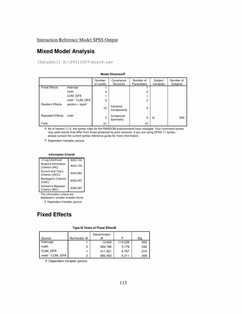
115

Interaction Reference Model SPSS Output


Model Dimensionb

1 1

3 2

1 1

3 2

10Variance

Components2

3Compound

Symmetry2 id 409

21 10

Intercept

meth

CUM_GPA

meth * CUM_GPA

Fixed Effects



Total

Number

of Levels

Covariance

Structure

Number of

Parameters

Subject

Variables

Number of

Subjects


may yield results that differ from those produced by prior versions. If you are using SPSS 11 syntax,

please consult the current syntax reference guide for more information.

a.



8323.724

8343.724

8343.963

8402.097

8392.097

-2 Log Likelihood


Criterion (AIC)

Hurvich and Tsai's

Criterion (AICC)


(CAIC)

Schwarz's Bayesian

Criterion (BIC)




Fixed Effects


1 13.628 114.228 .000

2 684.786 3.179 .042

1 411.521 6.767 .010

2 682.463 5.211 .006

Source

Intercept

meth

CUM_GPA

meth * CUM_GPA

Numerator df

Denominator

df F Sig.


116


45.733363 4.889838 31.965 9.353 .000 35.772658 55.694068

-13.2455 6.371821 698.064 -2.079 .038 -25.755755 -.735296

2.517373 5.597878 636.755 .450 .653 -8.475160 13.509905

0a 0 . . . . .

-.027802 1.339303 925.067 -.021 .983 -2.656226 2.600622

6.536750 2.150487 695.516 3.040 .002 2.314524 10.758975

.533492 1.913792 635.409 .279 .781 -3.224630 4.291613

0a 0 . . . . .

ParameterIntercept

[meth=1]

[meth=2]

[meth=3]

CUM_GPA

[meth=1] * CUM_GPA

[meth=2] * CUM_GPA

[meth=3] * CUM_GPA






421.6908 25.141290

12.426712 16.570487

17.919485 12.246745

18.385879 16.741821


CS covariance

Repeated Measures

Variancesection

Variancetopic

Estimate Std. Error


117

REFERENCES

Addelman, S. (1970). Variability of treatment and experiment units in the design and analysis of experiments. Journal of the American Statistical Association, 65, 1095-1108.

Alsop, R. (2006). Schools Find Fun A Worthy Teacher To Foster Creativity. Wall Street

Journal - Eastern Edition, 248(61), B8. Anselmi, K., & Frankel, R. (2004). Modular Experiential Learning for Business-to-

Business Marketing Courses. Journal of Education for Business, 79(3), 169-175. Auster, E. R., & Wylie, K. K. (2006). Creating Active Learning in the Classroom: A

Systematic Approach. Journal of Management Education, 30(2), 333-353. Barak, M., Lipson, A., & Lerman, S. (2006). Wireless Laptops as Means For Promoting

Active Learning In Large Lecture Halls. Journal of Research on Technology in

Education, 38(3), 245-263. Becker, W. E. (1997). Teaching Economics to Undergraduates. Journal of Economic

Literature, 35, 1347-1373. Blair, C., & Higgins, J. (1986). Comment on "Statistical Power with Group Mean as the

Unit of Analysis". Journal of Educational Statistics, 11(2), 161-169. Bloom, B. S. (1956). Taxonomy of educational objectives: The classification of

educational goals. White Plains, NY: Longman. Bonwell, C. C. (1997). Using active learning as assessment in the postsecondary

classroom. Clearing House, 71(2), 73. Bonwell, C. C., & Eison, J. A. (1991). Active learning : creating excitement in the

classroom Washington, DC School of Education and Human Development, George Washington University.

Bonwell, C. C., & Sutherland, T. E. (1996). The active learning continuum: Choosing activities to engage students in the classroom. New Directions for Teaching &

Learning(67), 3. Brown, R., & Guilding, C. (1993). A survey of teaching methods employed in

university business school accounting courses. Accounting Education, 2(3), 211-218.

Burstein, L. (1980). The Analysis of Multilevel Data in Educational Research and Evaluation. Review of Research in Education, 8, 158-233.

Casella, G., & Berger, R. L. (2002). Statistical Inference. North Scituate, MA: Duxbury Press.

Davey, C. L., Powell, J. A., Powell, J. E., & Cooper, I. (2002). Action learning in a medium-sized construction company. Building Research & Information, 30(1), 5-15.

Dean, A. M., & Voss, D. (1999). Design and Analysis of Experiments: Springer.

118

Donner, A. (1982). An Empirical Study of Cluster Randomization. International

Journal of Epidemiology, 11(3), 283-286. Donner, A. (1998). Some Aspects of the Design and Analysis of Cluster Randomization

Trials. Applied Statistics, 47(1), 95-113. Dunn, R. (1983). Learning style and its relation to exceptionality at both ends of the

specturn. Exceptional Children, 49, 496-506. Fai, A. H., & Cornelius, P. L. (1996). Approximate F-tests of multiple degree of

freedom hypothesis in generalized least squares analysis of unbalanced split-plot experiments. Journal of Statistical Computing and Simulation, 54, 363-378.

Fleming, N. D., & Mills, C. (1992). Not Another Inventory, Rather a Catalyst for Reflection. To Improve the Academy, 11, 137-143.

Garfield, J. (1993). Teaching Statistics Using Small-Group Cooperative Learning. Journal of Statistics Education, 1(1).

Glass, G., & Stanley, J. (1970). Statistical methods in education and psychology. Englewood Cliffs, N.J.: Printice-Hall.

Goldstein, H. (1991). Better Ways to Compare Schools? Journal of Educational

Statistics, 16(2), 89-91. Hair, J. F., Anderson, R. E., & Tatham, R. L. (1987). Multivariate Data Analysis. New

York: Macmillan. Hansen, J. D. (2006). Using Problem-Based Learning in Accounting. Journal of

Education for Business, 81(4), 221-224. Hedeker, Gibbons, & Flay. (1994). Random-Effects Regression Models for Clustered

Data with an Example from Smoking Prevention Research. Journal of

Consulting and Clinical Psychology, 62(4), 757-765. Hill, H., Rowan, B., & Ball, D. (2005). Effects of Teachers' Mathematical Knowledge

for Teaching on Student Achievement. American Educational Research Journal,

42(2), 371-406. Hillmer, S. C. (1996). A problem-solving approach to teaching business statistics.

American Statistician, 50(3), 249. Hopkins, K. (1982). The Unit of Analysis: Group Means Versus Individual

Observations. American Educational Research Journal, 19(1), 5-18. Kirschner, P. A., Sweller, J., & Clark, R. E. (2006). Why Minimal Guidance During

Instruction Does Not Work: An Analysis of the Failure of Constructivist, Discovery, Problem-Based, Experiential, and Inquiry-Based Teaching. Educational Psychologist, 41(2), 75-86.

Klahr, D., & Nigam, M. (2004). The equivalence of learning paths in early science instruction: Effects of direct instruction and discovery learning. Psychology

Science, 15, 661-667. Kvam, P. H. (2000). The Effect of Active Learning Methods on Student Retention in

Engineering Statistics. The American Statistician, 54(2), 136-140. Laverie, D. A. (2006). In-Class Active Cooperative Learning: A Way to Build

Knowledge and Skills in Marketing Courses. Marketing Education Review,

16(2), 59-76.

119

Li, T., Greenberg, B. A., & Nicholls, J. A. F. (2007). Teaching Experiential Learning: Adoption of an Innovative Course in an MBA Marketing Curriculum. Journal of

Marketing Education, 29(1), 25-33. Little, R., & Rubin, D. (2002). Statisitical Analysis with Missing Data: John Wiley &

Sons. Mayer, R. (2004). Should there be three-strikes rule against pure discovery learning?

The case for guided methods of instruction. American Psychologist, 59, 14-19. Moerbeek, M. (2005). Randomization of Clusters Versus Randomization of Persons

Within Clusters: Which is Preferable? American Statistical Association, 59(2), 173-179.

Moerbeek, M., Breukelen, G., & Berger, M. (2000). Design Issues for Experiments in Multilevel Populations. Journal of Behaviorial Statistics, 25(3), 271-284.

Morrell, C. H., Pearson, J. D., & Brant, L. J. (1997). Linear Transformations of Linear Mixed Effects Models. The American Statistician, 51(4).

Moulton, B. (1990). An Illustration of a Pitfall in Estimating the Effects of Aggregate Variables on Micro Units. The Review of Economics and Statistics, 72(2), 334-338.

Mumford, A. (1993). Action Learning: A Practitioner's Guide. Industrial & Commercial

Training, 25(10), v-vi. Mumford, A., & Honey, P. (1992). Questions and Answers on Learning Styles

Questionnaire. Industrial & Commercial Training, 24(7), 10. Neter, J., Kutner, M., Nachtsheim, C., & Wasserman, W. (1996). Applied Linear

Statistical Models: Irwin. O'Brien, E. M., & Hart, S. (1999). Action Learning: The link between academia and

industry? Educational Research, 41, 77-89. Page, D., & Mukherjee, A. (2000). Improving undergraduate student involvement in

management science and business writing courses using the seven principles in action. Education, 120, 547-557.

Patterson, H. D., & Thompson, R. (1971). Recovery of inter-block information when block sizes are unequal. Biometrika, 58(545).

Paul, P., & Mukhopadhyay, K. (2001). Using Information Technology for Active Learning in International Business Education. Marketing Education Review,

11(3), 81-89. Paul, P., & Mukhopadhyay, K. (2004). Experiental Learning in International Business

Education. Journal of Teaching in International Business, 16(2), 7-25. Pell, G. (2001). Action learning vs. traditional learning in a management development

context: a longitudinal study of MBA candidates. The International Journal of

Management Education, 35-48. Pfeffer, J., & Fong, C. T. (2002). The end of business schools? Less success than meets

the eye. Academy of Management Learning & Education, 1, 78-95. Pinheiro, J. C., & Bates, D. M. (2000). Mixed-Effects Models in S and S-PLUS. Berlin:

Springer-Verlag.

120

Raelin, J., & Coghlan, D. (2006). Developing Managers as Learners and Researchers: Using Action Learning and Action Research. Journal of Management

Education, 30(5), 670-689. Reinhardt, G., & Cook, L. S. (2006). Is This a Game or a Learning Moment? Decision

Sciences Journal of Innovative Education, 4(2), 301-304. Reinhardt, H. (1976). One picture is worth a thousand words? Not necessarily. Modern

Language Journal, 60, 160-168. Revans, R. (1971). Developing Effective Managers. London: Longman. Revans, R. (1983). Action Learning, Its Terms and Character. Management Decision,

21(1). Revans, R. W. (1971). Developing effective managers; a new approach to business

education: Praeger Publishers. Roth, H. P. (2005). An Active Learning Exercise Illustrating A Manufacturing Process

in A Cost Management Class. Decision Sciences Journal of Innovative

Education, 3(2), 367-374. Sarason, Y., & Banbury, C. (2004). Active Learning Facilitated by Using a Game-Show

Format Or Who Doesn't Want to be a Millionaire? Journal of Management

Education, 28(4), 509-518. Schneider, M. (2001, March 26). MBAs for working stiffs: Growing demand has

schools beefing up part-time programs. Business Week. Sims, B. (2006). Creating a Teaching and Learning Environment in Criminal Justice

Courses that Promotes Higher Order Thinking. Journal of Criminal Justice

Education, 17(2), 336-357. Stark, S. (2006). Using action learning for professional development. Educational

Action Research, 14(1), 23-43. Sutherland, T. E., & Bonwell, C. C. (1996). Using Active Learning in College Classes:

A Range of Options for Faculty (Vol. 67). Sweller, J. (2003). Evolution of human cognitive architecture. In B. Ross (Ed.). The

psychology of learning and motivation, 43, 215-266. Ueltschy, L. C. (2001). An Exploratory Study of Integrating Interactive Technology

into the Marketing Curriculum. Journal of Marketing Education, 23(1), 63-72. Umble, M., & Umble, E. J. (2004). Using Active Learning to Transform the Monte Hall

Problem into an Invaluable Classroom Exercise. Decision Sciences Journal of

Innovative Education, 2(2), 213-217. Verbeke, G., & Molenberghs, G. (1997). Linear Mixed Models in Practice. New York:

Springer-Verlag Verbeke, G., & Molenberghs, G. (2000). Linear Mixed Models for Longitudinal Data.

Berlin: Springer-Verlag. Vince, R., & Martin, L. (1993). Inside Action Learning: An Exploration of the

Psychology and Politics of the Action Learning Model. Management Education

and Development, 24(3), 204-215. West, B., Welch, K., & Galecki, A. (2007). Linear Mixed Models: A Practical Guide

Using Statistical Software. Boca Raton: Chapman & Hall.

121

Woodruff, S. (1997). Random-Effects Models for Analyzing Clustered Data from a Nutrition Education Intervention. Evaluation Review, 21(6), 688-697.

Yolanda, S., & Catherine, B. (2004). Active Learning Facilitated by Using a Game-Show Format or Who Doesn't Want to be a Millionaire? Journal of Management

Education, 28(4), 509-518.

122

BIOGRAPHICAL INFORMATION

Prior to completing the Ph.D., David spent sixteen years in the

technology industry with a wide range of experience in marketing, consulting, and

academic positions. He has demonstrated success in matching client business

requirements with appropriate technology solutions. David has received a number of

awards for leadership in technology sales and financial justification of information

based solutions. Much of David’s career has been working with distribution industry

clients. Organizations David has held long-term positions with include; IBM

Corporation, The M.J. Neeley School of Business at Texas Christian University, and

The University of Texas at Arlington. David received the Master of Science degree in

Operations Research from Southern Methodist University in 1986, a Master of Science

degree in Information Systems from UTA as well as the Ph.D. in Business Statistics.

David has received a number of university teaching awards and his research interests

include; teaching methods, active learning, logistics, and applied statistical

methodologies.

A COMPARISION OF TRADITIONAL AND ACTIVE LEARNING …

Documents

Transcript of A COMPARISION OF TRADITIONAL AND ACTIVE LEARNING …