atmosphere

Article

A Commercial Aircraft Fuel Burn and EmissionsInventory for 2005–2011

Donata K. Wasiuk 1, Md Anwar H. Khan 2, Dudley E. Shallcross 2 and Mark H. Lowenberg 1,*1 Department of Aerospace Engineering, Queen’s Building, University Walk, University of Bristol,

Bristol BS8 1TR, UK; donataw@gmail.com2 Atmospheric Chemistry Research Group, School of Chemistry, Cantock’s Close, University of Bristol,

Bristol BS8 1TS, UK; anwar.khan@bristol.ac.uk (M.A.H.K.); d.e.shallcross@bristol.ac.uk (D.E.S.)* Correspondence: m.lowenberg@bristol.ac.uk; Tel.: +44-117-331-5555

Academic Editor: Robert W. TalbotReceived: 11 April 2016; Accepted: 27 May 2016; Published: 4 June 2016

Abstract: The commercial aircraft fuel burn and emission estimates of CO2, CO, H2O, hydrocarbons,NOx and SOx for 2005–2011 are given as the 4-D Aircraft Fuel Burn and Emissions Inventory.On average, the annual fuel burn and emissions of CO2, H2O, NOx, and SOx increased by 2%–3%for 2005–2011, however, annual CO and HC emissions decreased by 1.6% and 8.7%, respectivelybecause of improving combustion efficiency in recent aircraft. Approximately 90% of the globalannual aircraft NOx emissions were emitted in the NH between 2005 and 2011. Air traffic withinthe three main industrialised regions of the NH (Asia, Europe, and North America) alone accountedfor 80% of the global number of departures, resulting in 50% and 45% of the global aircraft CO2

and NOx emissions, respectively, during 2005–2011. The current Asian fleet appears to impact ourclimate strongly (in terms of CO2 and NOx) when compared with the European and North Americanfleet. The changes in the geographical distribution and a gradual shift of the global aircraft NOx

emissions as well as a subtle but steady change in regional emissions trends are shown in particularcomparatively rising growth rates between 0 and 30˝N and decreasing levels between 30 and 60˝N.

Keywords: global and regional aviation; fuel burn; aircraft NOx emissions; geographical distribution

1. Introduction

The emissions of carbon dioxide (CO2), nitrogen oxide (NOx), sulphur oxide (SOx), carbonmonoxide (CO), water vapour (H2O), and hydrocarbons (HC) from aircraft can have a significantimpact on the atmosphere by changing its oxidising capacity and hence the greenhouse gas removalrates, by increasing the levels of greenhouse gases, and by forming particles, contrails, and cirruscloud [1–10]. Aircraft emissions have increased over time due to high, sustained, and rising levelsof passenger traffic driven by continued economic growth and reduced air fares. Airbus predicts adoubling in the level of demand in the next 15 years [11]. Among the aircraft emissions, the emissionsof the long-lived well-mixed greenhouse gas, CO2, represent 2.0% to 2.5% of total annual CO2

emissions [3]. The impact of CO2 on climate is independent of location due to its long atmosphericlife-time of over 100 years. In recent years, the aircraft emissions of CO2 have become a contentiousissue and market based measures (e.g., emission trading, emission related levies, and emissionoffsetting) have been introduced in certain parts of the world that aim to assign a price to theenvironmental cost of CO2 emissions from aircraft. Hence, the EU Emissions Trading System (ETS)was implemented within the European Economic Area (EEA), the 28 EU member states, plus Iceland,Liechtenstein, and Norway [12].

The emissions of NOx from aircraft have an indirect effect on our climate because of the productionof a very potent greenhouse gas, O3, from the reactions of hydrocarbons and NOx in the presence

Atmosphere 2016, 7, 78; doi:10.3390/atmos7060078 www.mdpi.com/journal/atmosphere

Atmosphere 2016, 7, 78 2 of 14

of ultra-violet light. The chemical production of O3 per NOx molecule emitted by an aircraft is anon-linear function of ambient levels of NOx [13] and the availability of HOx from the photo-oxidationof non-methane hydrocarbons [14,15], both factors depending largely on altitude. Hence, the impactof aircraft NOx emissions, unlike that of CO2, is dependent on the location of the emissions [16,17].Near ground level during aircraft take-off, landing, taxi-in, taxi-out, the aircraft are in low powercondition leading to higher emissions of CO, NOx, HC which may induce smog formation and haze.Aviation SOx may play a role in the environment by the development of acid rain and the formationof sulphate aerosol particles [18]. Under some meteorological conditions, the presence of aviationinduced H2O, sulphate particles can form contrails at high altitudes and promote formation of cirrusclouds, which may have an effect on climate change [2].

The estimation of aircraft CO2 and NOx emissions in the form of inventories is a crucial componentin the assessment of the atmospheric and climate impact of aviation. The inventories make up thebackbone of these assessments. To date, only a limited number of such inventories [8,19–34] have beenproduced. Most of the aircraft fuel burn and emissions inventories that were produced in the last twodecades cover a handful of years only and few have been able to analyse the trends over a significantnumber of years.

In this paper, the estimates from an up-to-date aircraft mission fuel burn and emissions inventoryare presented. The inventory is referred to as the 4-D Aircraft Fuel Burn and Emissions Inventory andit reflects as closely as possible the composition of the global fleet from 2005 to 2011. The inventory wascreated using a combination of air traffic data, aircraft performance data, and emissions calculationmethods [35]. Further, a global, 3-D distribution of aircraft NOx emissions was derived from theinventory for the time period 2005–2011. Because the estimates in the 4-D Aircraft Fuel Burn andEmissions Inventory were derived using one, self-consistent method, they present an illustrativehistorical trend analysis that narrates a story of markedly deviating growth and decline, and capturethe impact of the 2008 global economic crisis. The study also showed the relationship between theintracontinental volume of air traffic and the volume of fuel burn and emissions (measured in Tg)of CO2 and NOx accounted for by the intracontinental traffic within the regions Asia, Europe, andNorth America.

2. Methodology

2.1. 4-D Aircraft Fuel Burn and Emission Inventory Derivation

Aircraft Performance Model Implementation (APMI) software containing a database of globalaircraft movements, a model of aircraft performance for all phases of a flight, and the equations for thecalculation of aircraft emissions was used to estimate aircraft mission fuel burn, mission time, distance,and emissions from 2005 to 2011. The global and regional aircraft movements’ statistics from 2005 to2011 were obtained from the global airline schedules data, CAPSTATS (http://www.capstats.com/).Only the commercial, scheduled aircraft information were available in the database, neither militarynor non-scheduled traffic, such as business jets and charter flight were included in the database.Each flight was listed by city pair and airline and included the aircraft code and departures frequency.Out of the total 6,622,219 flights collected for the period of 2005 to 2011, each represents the monthlytotal number of departures on a particular route, made by a particular airline and using a particulartype of aircraft. If the same airline operated two different aircraft types on any given route during anygiven month between 2005 and 2011, the total monthly number of departures was recorded separatelyfor each of the different aircraft types operated by this airline on the same route. Different engineoptions on a particular aircraft type were also treated separately. The details of the sourcing of the flightrecords and their incorporation into the database can be found in Wasiuk et al. [35]. The CAPSTATSdatabase is similar to the air traffic data contained in OAG (http://www.oag.com/), but is much moreaffordable compared to the traditionally employed OAG. Thus the extracted CAPSTATS air traffic datawas compared with an excerpt of the OAG database for a single month, September 2008, and it was

Atmosphere 2016, 7, 78 3 of 14

found that 94% of the OAG data (the departure airport and country, destination airport and country,aircraft and airline code) matched with CAPSTATS data. There was a partial match for the remaining6% of the data rows present in OAG and not in CAPSTATS, with the only field not matching being theaircraft code [35].

The EUROCONTROL Experimental Centre (EEC) developed an aircraft performance model,BADA (Base of Aircraft Data), version 3.9 (http://www.eurocontrol.int/services/bada) of whichwas used to calculate the aircraft performance parameters for all stages of a typical aircraft mission.BADA contains performance and operating procedure data for 338 different aircraft, 117 of whichare directly supported. The remaining 221 aircraft are supported by the other models determined byEUROCONTROL. The details of the BADA model can be found in Wasiuk et al. [35]. A typical aircraftmission was divided into six stages: taxi out (TOUT), take-off (TO), climb (CL), cruise (CR), descent(DES), and taxi in (TIN). CL, CR, and DES were assigned fuel flow and fuel burn values for a givenaircraft, mission type and distance calculated by the BADA Total Energy Model (TEM). The TOUT,TO, TIN phases were modelled using engine specific fuel flow values taken from International CivilAviation Organization (ICAO) for jet aircraft [36] and from the Swedish Defence Research Agency(FOI) for turboprop aircraft [37]. The ground level emissions were estimated using ICAO specifiedtaxi times and thrust settings. The Operation Performance Model (OPM) of BADA gave the airframespecific performance parameters and the Airline Procedure Model (APM) of BADA gave airframeand airline specific speeds and Mach numbers which were used to calculate the thrust, drag, fuelflow, and fuel burn values at different stages of a typical aircraft mission. The detail of the modelincluding assumptions and limitations is given by Wasiuk et al. [35]. The implementation of themathematical model of aircraft performance was validated against EUROCONTROL performancetables (http://www.eurocontrol.int/services/bada).

The emissions of CO2, CO, NOx, SOx, H2O, and HC were estimated using the Boeing Fuel FlowMethod 2 (BFFM2) [38]. Aircraft performance data, reference emissions and fuel flows were used asinput to the method. The level of the emissions of CO2, CO, NOx, SOx, H2O, and HC is quantifiedby emission indices (EIs) that specify how many grams of the species are released per one kilogramof fuel burned. EIs are typically represented as a function of an engine power setting and a fuel flowrate. The detailed description of the emission calculation method can be found in Wasiuk et al. [35].The procedure for the calculation of aircraft emissions was validated against an SAE (Society ofAutomotive Engineers) long-haul flight example [39].

The trajectory simulation of each of the unique missions recorded in the air traffic movements’database with the APMI software assigned a mission distance, time, and fuel burn, a reservefuel requirement, and the emissions of CO2, CO, NOx, SOx, H2O, and HC to each unique flight.These quantities were multiplied by the total number of departures for the month and in this way themonthly totals were calculated. The monthly totals were summed to obtain the yearly estimates.

2.2. 3-D NOx Emissions Distribution Fields

The total global aircraft NOx emissions for each year between 2005 and 2011 were distributedon a grid with a resolution of 5˝ longitude ˆ 5˝ latitude. The vertical grid resolution followed thepressure levels and approximate height bands which are based on the vertical model resolution of the3-D STOCHEM-CRI chemistry and transport model [40,41]. The geographical location of each airportwas localised within a grid cell. Each unique route between origin airport (e.g., A) and destinationairport (e.g., B) was assigned a shortest path using a direct search algorithm. The algorithm assumedthat the mission was flown in a straight line between A and B and that A and B were positioned in themiddle of the grid cell in which they had been localised. The path was made up of the grid cells whichthis straight line crossed. Each unique rout was then assigned a number of levels based on the cruisealtitude attained during the mission simulated in the APMI. In the mission, TOUT and TIN took placewithin the grid cell of A and B respectively, CL took place in the column vertically above the grid cellof A until the CR level was reached and DES took place in the column vertically above the grid cell of

Atmosphere 2016, 7, 78 4 of 14

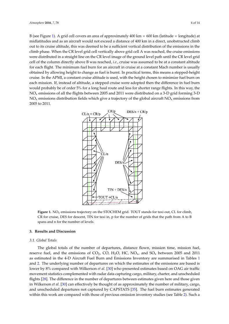
B (see Figure 1). A grid cell covers an area of approximately 400 km ˆ 600 km (latitude ˆ longitude) atmidlatitudes and as an aircraft would not exceed a distance of 400 km in a direct, unobstructed climbout to its cruise altitude, this was deemed to be a sufficient vertical distribution of the emissions in theclimb phase. When the CR level grid cell vertically above grid cell A was reached, the cruise emissionswere distributed in a straight line on the CR level image of the ground level path until the CR level gridcell of the column directly above B was reached, i.e., cruise was assumed to be at a constant altitudefor each flight. The minimum fuel burn for an aircraft in cruise at a constant Mach number is usuallyobtained by allowing height to change as fuel is burnt. In practical terms, this means a stepped-heightcruise. In the APMI, a constant cruise altitude is used, with the height chosen to minimize fuel burn oneach mission. If, instead of altitude, a stepped cruise were adopted then the difference in fuel burnwould probably be of order 5% for a long haul route and less for shorter range flights. In this way, theNOx emissions of all the flights between 2005 and 2011 were distributed on a 3-D grid forming 3-DNOx emissions distribution fields which give a trajectory of the global aircraft NOx emissions from2005 to 2011.

Atmosphere 2016, 7, 78 4 of 14

climb out to its cruise altitude, this was deemed to be a sufficient vertical distribution of the emissions

in the climb phase. When the CR level grid cell vertically above grid cell A was reached, the cruise

emissions were distributed in a straight line on the CR level image of the ground level path until the

CR level grid cell of the column directly above B was reached, i.e., cruise was assumed to be at a

constant altitude for each flight. The minimum fuel burn for an aircraft in cruise at a constant Mach

number is usually obtained by allowing height to change as fuel is burnt. In practical terms, this

means a stepped-height cruise. In the APMI, a constant cruise altitude is used, with the height chosen

to minimize fuel burn on each mission. If, instead of altitude, a stepped cruise were adopted then the

difference in fuel burn would probably be of order 5% for a long haul route and less for shorter range

flights. In this way, the NOx emissions of all the flights between 2005 and 2011 were distributed on a

3-D grid forming 3-D NOx emissions distribution fields which give a trajectory of the global aircraft

NOx emissions from 2005 to 2011.

Figure 1. NOx emissions trajectory on the STOCHEM grid. TOUT stands for taxi out, CL for climb,

CR for cruise, DES for descent, TIN for taxi in, p for the number of grids that the path from A to B

spans and n for the number of levels.

3. Results and Discussion

3.1. Global Totals

The global totals of the number of departures, distance flown, mission time, mission fuel, reserve

fuel, and the emissions of CO2, CO, H2O, HC, NOx, and SOx between 2005 and 2011 as estimated in

the 4-D Aircraft Fuel Burn and Emissions Inventory are summarised in Tables 1 and 2. The

underlying number of departures on which the estimates of the emissions are based is lower by 8%

compared with Wilkerson et al. [30] who presented estimates based on OAG air traffic movement

statistics complemented with radar data capturing cargo, military, charter, and unscheduled flights

[28]. The difference in the number of departures between estimates given here and those given in

Wilkerson et al. [30] can effectively be thought of as approximately the number of military, cargo, and

unscheduled departures not captured by CAPSTATS [35]. The fuel burn estimates generated within

this work are compared with those of previous emission inventory studies (see Table 2). Such a

comparison is limited both by the quality of the emission inventory, and the quality and availability

of fuel production data, as there is no perfect database with which to validate or evaluate the jet fuel

Figure 1. NOx emissions trajectory on the STOCHEM grid. TOUT stands for taxi out, CL for climb,CR for cruise, DES for descent, TIN for taxi in, p for the number of grids that the path from A to Bspans and n for the number of levels.

3. Results and Discussion

3.1. Global Totals

The global totals of the number of departures, distance flown, mission time, mission fuel,reserve fuel, and the emissions of CO2, CO, H2O, HC, NOx, and SOx between 2005 and 2011as estimated in the 4-D Aircraft Fuel Burn and Emissions Inventory are summarised in Tables 1and 2. The underlying number of departures on which the estimates of the emissions are based islower by 8% compared with Wilkerson et al. [30] who presented estimates based on OAG air trafficmovement statistics complemented with radar data capturing cargo, military, charter, and unscheduledflights [28]. The difference in the number of departures between estimates given here and those givenin Wilkerson et al. [30] can effectively be thought of as approximately the number of military, cargo,and unscheduled departures not captured by CAPSTATS [35]. The fuel burn estimates generatedwithin this work are compared with those of previous emission inventory studies (see Table 2). Such a

Atmosphere 2016, 7, 78 5 of 14

comparison is limited both by the quality of the emission inventory, and the quality and availabilityof fuel production data, as there is no perfect database with which to validate or evaluate the jet fuelconsumption data [23,24,42]. Nevertheless, the International Energy Agency (IEA) publishes yearlyfigures of the total global crude oil production, as well as the total global jet kerosene production.It estimates that in 2009 the total global crude oil production was 3518.5 Tg, while the total globaljet kerosene production was 233.6 Tg, constituting 6.6% of the total global crude oil production [43].This figure does not take into account jet fuel production from coal (synthetic jet fuel) which could besignificant in some regions (e.g., South Africa).

The fuel match is defined as the ratio of the fuel consumption estimate from an inventory andthe global supply of aviation fuel [42]. Using our estimation of the global total fuel use for the year2009, we calculated the fuel match as 258.4/233.6 = 1.1, a 10% overestimate. This overestimationmay depend on the fact that the IEA relies on reported information. Total fuel use, including theestimated mission fuel burn and reserve fuel requirement was adopted for the calculation described.Using the estimated mission fuel burn only, the fuel match is 0.68, an underestimate of 32%, takinginto account that mission fuel burn was estimated with flight trajectory simulations optimising forleast fuel burn. It is most likely that the actual fuel use figure falls somewhere between these twoextremes, i.e., a fuel use figure with a reserve fuel allowance and a fuel burn figure with no reserve fuelallowance. Military aviation and cargo could be the significant source of global aircraft fuel [27,30]which was not considered in the fuel consumption estimate resulting in underestimating the missionfuel burn in this study.

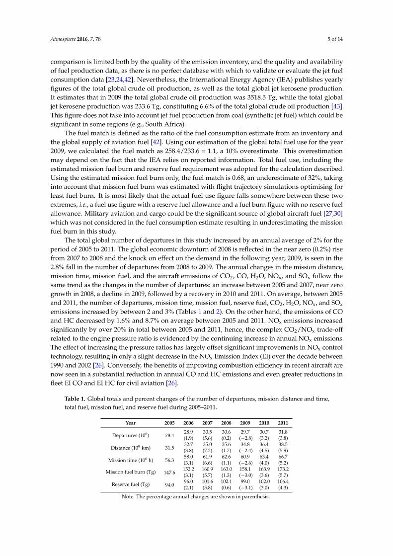
The total global number of departures in this study increased by an annual average of 2% for theperiod of 2005 to 2011. The global economic downturn of 2008 is reflected in the near zero (0.2%) risefrom 2007 to 2008 and the knock on effect on the demand in the following year, 2009, is seen in the2.8% fall in the number of departures from 2008 to 2009. The annual changes in the mission distance,mission time, mission fuel, and the aircraft emissions of CO2, CO, H2O, NOx, and SOx follow thesame trend as the changes in the number of departures: an increase between 2005 and 2007, near zerogrowth in 2008, a decline in 2009, followed by a recovery in 2010 and 2011. On average, between 2005and 2011, the number of departures, mission time, mission fuel, reserve fuel, CO2, H2O, NOx, and SOx

emissions increased by between 2 and 3% (Tables 1 and 2). On the other hand, the emissions of COand HC decreased by 1.6% and 8.7% on average between 2005 and 2011. NOx emissions increasedsignificantly by over 20% in total between 2005 and 2011, hence, the complex CO2/NOx trade-offrelated to the engine pressure ratio is evidenced by the continuing increase in annual NOx emissions.The effect of increasing the pressure ratios has largely offset significant improvements in NOx controltechnology, resulting in only a slight decrease in the NOx Emission Index (EI) over the decade between1990 and 2002 [26]. Conversely, the benefits of improving combustion efficiency in recent aircraft arenow seen in a substantial reduction in annual CO and HC emissions and even greater reductions infleet EI CO and EI HC for civil aviation [26].

Table 1. Global totals and percent changes of the number of departures, mission distance and time,total fuel, mission fuel, and reserve fuel during 2005–2011.

Year 2005 2006 2007 2008 2009 2010 2011

Departures (106) 28.428.9 30.5 30.6 29.7 30.7 31.8(1.9) (5.6) (0.2) (´2.8) (3.2) (3.8)

Distance (109 km) 31.532.7 35.0 35.6 34.8 36.4 38.5(3.8) (7.2) (1.7) (´2.4) (4.5) (5.9)

Mission time (106 h) 56.358.0 61.9 62.6 60.9 63.4 66.7(3.1) (6.6) (1.1) (´2.6) (4.0) (5.2)

Mission fuel burn (Tg) 147.6152.2 160.9 163.0 158.1 163.9 173.2(3.1) (5.7) (1.3) (´3.0) (3.6) (5.7)

Reserve fuel (Tg) 94.096.0 101.6 102.1 99.0 102.0 106.4(2.1) (5.8) (0.6) (´3.1) (3.0) (4.3)

Note: The percentage annual changes are shown in parenthesis.

Atmosphere 2016, 7, 78 6 of 14

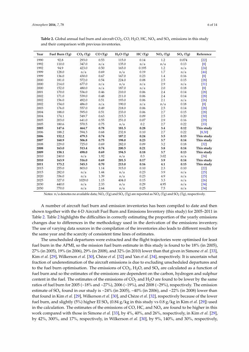
Table 2. Global annual fuel burn and aircraft CO2, CO, H2O, HC, NOx and SOx emissions in this studyand their comparison with previous inventories.

Year Fuel Burn (Tg) CO2 (Tg) CO (Tg) H2O (Tg) HC (Tg) NOx (Tg) SOx (Tg) Reference

1990 92.8 293.0 0.53 115.0 0.14 1.2 0.074 [22]1992 110.0 347.0 n/a 135.0 n/a n/a 0.13 [8]1992 94.9 423.0 0.50 165.0 0.195 1.2 n/a [24]1999 128.0 n/a 0.69 n/a 0.19 1.7 n/a [44]1999 136.0 430.0 0.67 167.0 0.23 1.4 0.16 [8]2000 181.0 572.0 0.54 224.0 0.08 2.5 0.15 [28]2000 214.0 677.0 n/a n/a n/a 2.9 n/a [31]2000 152.0 480.0 n/a 187.0 n/a 2.0 0.18 [8]2001 170.0 536.0 0.46 210.0 0.06 2.4 0.14 [28]2002 171.0 539.0 0.48 211.0 0.06 2.4 0.14 [28]2002 156.0 492.0 0.51 193.0 0.06 2.1 n/a [26]2002 154.0 486.0 n/a 190.0 n/a n/a 0.18 [8]2003 176.0 557.0 0.49 218.0 0.06 2.5 0.14 [28]2004 188.0 595.0 0.51 233.0 0.06 2.7 0.15 [28]2004 174.1 549.7 0.63 215.3 0.09 2.5 0.20 [30]2005 203.0 641.0 0.55 251.0 0.07 2.9 0.16 [29]2005 180.6 570.5 0.75 n/a 0.2 2.7 0.22 [33]2005 147.6 464.7 0.78 181.5 0.28 3.4 0.12 This study2006 188.2 594.3 0.68 232.8 0.10 2.7 0.22 [8,30]2006 152.2 479.3 0.74 187.2 0.24 3.5 0.13 This study2007 160.9 506.8 0.75 198.0 0.23 3.7 0.14 This study2008 229.0 725.0 0.69 282.0 0.09 3.2 0.18 [32]2008 163.0 513.4 0.74 200.5 0.21 3.8 0.14 This study2009 158.1 498.0 0.69 194.5 0.18 3.7 0.13 This study2010 240.0 n/a 1.92 n/a 0.3 3.02 n/a [34]2010 163.9 516.0 0.69 201.5 0.17 3.9 0.14 This study2011 173.2 545.3 0.70 213.0 0.16 4.1 0.15 This study2015 255.0 803.0 1.14 315.0 0.10 2.3 0.10 [22]2015 282.0 n/a 1.44 n/a 0.23 3.9 n/a [25]2020 336.0 n/a 1.39 n/a 0.23 4.9 n/a [25]2025 327.0 1029.0 1.15 404.0 0.15 3.3 n/a [26]2030 440.0 n/a 2.33 n/a 0.29 4.95 n/a [34]2050 770.0 n/a 2.64 n/a 0.25 7.5 n/a [34]

Notes: n/a denotes no available data; NOx (Tg) and SOx (Tg) are reported as NO2 (Tg) and SO2 (Tg), respectively.

A number of aircraft fuel burn and emission inventories has been compiled to date and thenshown together with the 4-D Aircraft Fuel Burn and Emissions Inventory (this study) for 2005–2011 inTable 2. Table 2 highlights the difficulties in correctly estimating the proportion of the yearly emissionschanges due to differences in the methodology used in the derivation of the emissions inventory.The use of varying data sources in the compilation of the inventories also leads to different results forthe same year and the scarcity of consistent time lines of estimates.

The unscheduled departures were extracted and the flight trajectories were optimised for leastfuel burn in the APMI, so the mission fuel burn estimate in this study is found to be 18% (in 2005),27% (in 2005), 19% (in 2006), 29% (in 2008), and 32% (in 2010) lower than that given in Simone et al. [33],Kim et al. [29], Wilkerson et al. [30], Chèze et al. [32] and Yan et al. [34], respectively. It is uncertain whatfraction of underestimation of the aircraft emissions is due to excluding unscheduled departures andto the fuel burn optimisation. The emissions of CO2, H2O, and SOx are calculated as a function offuel burn and so the estimates of the emissions are dependent on the carbon, hydrogen and sulphurcontent in the fuel. The estimates of the emissions of CO2 and H2O are found to be lower by the sameratios of fuel burn for 2005 (~18% and ~27%), 2006 (~19%), and 2008 (~29%), respectively. The emissionestimate of SOx found in our study is ~24% (in 2005), ~40% (in 2006), and ~22% (in 2008) lower thanthat found in Kim et al. [29], Wilkerson et al. [30], and Chèze et al. [32], respectively because of the lowerfuel burn, and slightly (5%) higher EI SOx (0.84 g/kg in this study vs 0.8 g/kg in Kim et al. [29]) usedin the calculation. The estimates of the emissions of CO, HC, and NOx are found to be higher in thiswork compared with those in Simone et al. [33], by 4%, 40%, and 26%, respectively, in Kim et al. [29],by 42%, 300%, and 17%, respectively, in Wilkerson et al. [30], by 9%, 140%, and 30%, respectively,

Atmosphere 2016, 7, 78 7 of 14

and in Chèze et al. [32], by 7%, 133%, and 19%, respectively. The emissions of CO, HC, and NOx

are calculated as a function of fuel burned, altitude, and engine type. As these emissions do notdepend on the mission fuel burn alone, hence not on the number of departures modelled, there areother reasons (e.g., airframe/engine match, the use of ICAO prescribed taxi in and taxi out times,reduced thrust take-off, the use of different data sources for turboprop engine fuel flow and EI data,modelling a large number of jet engines which exhibit a non-standard behaviour with respect to EICOand EIHC, and errors associated with modelling EICO and EIHC below the 7% power setting) forthese differences. Care would need to be exercised in extending the current methodology to neweraircraft with staged combustor engines, since the Boeing Fuel Flow method used to assign emissionsestimates from the APMI results is not appropriate for engines with such combustors [35]. However,the inventory generated within this work is helpful in extending this timeline with estimates based ona self-consistent method.

3.2. Global Vertical Profiles

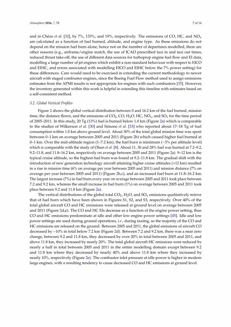
Figure 2 shows the global vertical distribution between 0 and 16.2 km of the fuel burned, missiontime, the distance flown, and the emissions of CO2, CO, H2O, HC, NOx, and SOx for the time periodof 2005–2011. In this study, 20 Tg (13%) fuel is burned below 1.0 km (Figure 2a) which is comparableto the studies of Wilkerson et al. [30] and Simone et al. [33] who reported about 17–18 Tg of fuelconsumption within 1.0 km above ground level. About 30% of the total global mission time was spentbetween 0–1 km on average between 2005 and 2011 (Figure 2b) which caused higher fuel burned at0–1 km. Over the mid-altitude region (1–7.2 km), the fuel burn is minimum (~3% per altitude level)which is comparable with the study of Olsen et al. [8]. About 11, 30 and 28% fuel was burned at 7.2–9.2,9.2–11.8, and 11.8–16.2 km, respectively on average between 2005 and 2011 (Figure 2a). 9–12 km is thetypical cruise altitude, so the highest fuel burn was found at 9.2–11.8 km. The gradual shift with theintroduction of new generation technology aircraft attaining higher cruise altitudes (>12 km) resultedin a rise in mission time (6% on average per year between 2005 and 2011) and mission distance (7% onaverage per year between 2005 and 2011) (Figure 2b,c), and an increased fuel burn at 11.8–16.2 km.The largest increase (7%) in fuel burn every year on average between 2005 and 2011 took place between7.2 and 9.2 km, whereas the small increase in fuel burn (1%) on average between 2005 and 2011 tookplace between 9.2 and 11.8 km (Figure 2a).

The vertical distributions of the global total CO2, H2O, and SOx emissions qualitatively mirrorthat of fuel burn which have been shown in Figures S1, S2, and S3, respectively. Over 40% of thetotal global aircraft CO and HC emissions were released at ground level on average between 2005and 2011 (Figure 2d,e). The CO and HC EIs decrease as a function of the engine power setting, thusCO and HC emissions predominate at idle and other low engine power settings [45]. Idle and lowpower settings are used during ground operations, i.e., during taxiing, so the majority of the CO andHC emissions are released on the ground. Between 2005 and 2011, the global emissions of aircraft COdecreased by ~10% in total below 7.2 km (Figure 2d). Between 7.2 and 9.2 km, there was a near zerochange, between 9.2 and 11.8 km, they decreased by over 20% in total between 2005 and 2011, andabove 11.8 km, they increased by nearly 20%. The total global aircraft HC emissions were reduced bynearly a half in total between 2005 and 2011 in the entire modelling domain except between 9.2and 11.8 km where they decreased by nearly 40% and above 11.8 km where they increased bynearly 10%, respectively (Figure 2e). The combustor inlet pressure at idle power is higher in modernlarge engines, with a resulting tendency to cause decreased CO and HC emissions at ground level.

Atmosphere 2016, 7, 78 8 of 14

Atmosphere 2016, 7, 78 8 of 14

respectively (Figure 2e). The combustor inlet pressure at idle power is higher in modern large

engines, with a resulting tendency to cause decreased CO and HC emissions at ground level.

Figure 2. Vertical distribution of the global total (a) mission fuel burn, (b) mission time, (c) mission

distance, (d) CO emissions, (e) HC emissions, and (f) NOx emissions during 2005–2011

Aircraft NOx emissions occur primarily at high engine power settings, hence during take-off and

during the cruise portion of a flight [44], thus ~80% of the total global annual aircraft NOx emissions

was distributed between 7.2 and 16.2 km during the period of 2005–2011 (Figure 2f). In 2005 and 2006,

the highest fraction (over one-third) of the total global annual aircraft NOx emissions was released at

an altitude between 9.2 and 11.8 km and from 2007 onwards between 11.8 and 16.2 km which is the

most pronounced change in the vertical distribution (see Figure 2f). This could be due to a shift to

aircraft types that are able to attain higher cruise altitudes from 2007 onwards. The changes in the

amount of NOx emitted between 9.2 and 11.8 km on average between 2005 and 2011 was significantly

below the global average, despite the fact that the second highest proportion of the total global annual

aircraft NOx emissions were deposited between these altitudes. The highest rise (7.7%) took place

above 11.8 km on average between 2005 and 2011, nearly double the global average.

3.3. Spatial Distribution of Global Aircraft NOx Emissions

The average (2005–2011) spatial distribution of the total global NOx emissions from aircraft

between 5.6 and 16.2 km (Figure 3) highlights the areas of activity and major global flight paths.

Approximately 90% of the total global annual aircraft NOx emissions was allocated to the northern

hemisphere (NH) on average between 2005 and 2011 for all altitudes from 0 to 16.2 km. During this

period, the highest proportion, approximately one-third, of the NOx emissions allocated to the NH

was found between 30°N and 40°N. Nearly 90% of all the NOx allocated to the NH was emitted

between 20°N and 60°N (Figure 4). Two features of the distribution of the annual aircraft NOx

emissions in the NH between 2005 and 2011 were highlighted by the inventory. The first feature is a

small but consistent decline in the fraction emitted between 30°N and 60°N (Figure 4). 30°N coincides

with the southern border of the US, while 49°N coincides with the northern border of the USA.

Europe except Scandinavia and Iceland is contained within these latitudes. Secondly, and conversely,

there is a small but consistent rise in this share between 0°N and 30°N (Figure 4). The 0–30°N latitude

belt covers South Asia. This points to a subtle shift in the distribution of the annual aircraft NOx

emissions in the NH.

Figure 2. Vertical distribution of the global total (a) mission fuel burn, (b) mission time, (c) missiondistance, (d) CO emissions, (e) HC emissions, and (f) NOx emissions during 2005–2011.

Aircraft NOx emissions occur primarily at high engine power settings, hence during take-off andduring the cruise portion of a flight [44], thus ~80% of the total global annual aircraft NOx emissionswas distributed between 7.2 and 16.2 km during the period of 2005–2011 (Figure 2f). In 2005 and 2006,the highest fraction (over one-third) of the total global annual aircraft NOx emissions was releasedat an altitude between 9.2 and 11.8 km and from 2007 onwards between 11.8 and 16.2 km which isthe most pronounced change in the vertical distribution (see Figure 2f). This could be due to a shiftto aircraft types that are able to attain higher cruise altitudes from 2007 onwards. The changes in theamount of NOx emitted between 9.2 and 11.8 km on average between 2005 and 2011 was significantlybelow the global average, despite the fact that the second highest proportion of the total global annualaircraft NOx emissions were deposited between these altitudes. The highest rise (7.7%) took placeabove 11.8 km on average between 2005 and 2011, nearly double the global average.

3.3. Spatial Distribution of Global Aircraft NOx Emissions

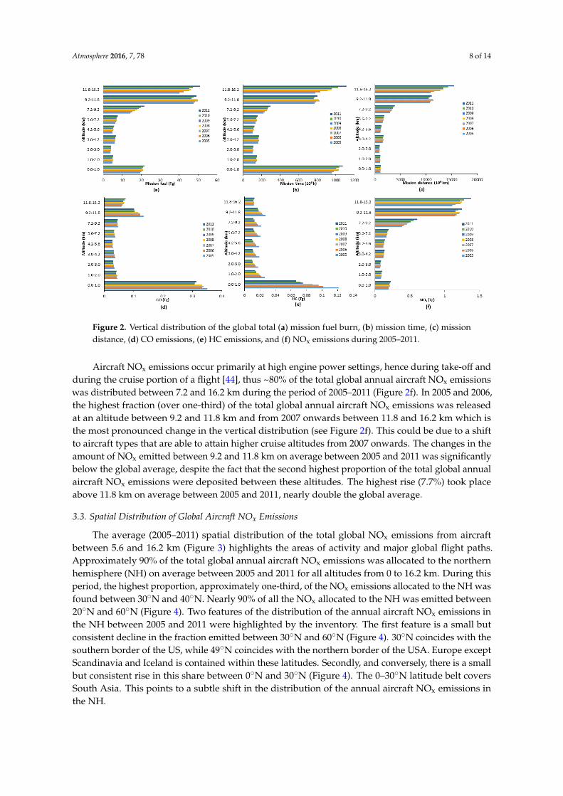
The average (2005–2011) spatial distribution of the total global NOx emissions from aircraftbetween 5.6 and 16.2 km (Figure 3) highlights the areas of activity and major global flight paths.Approximately 90% of the total global annual aircraft NOx emissions was allocated to the northernhemisphere (NH) on average between 2005 and 2011 for all altitudes from 0 to 16.2 km. During thisperiod, the highest proportion, approximately one-third, of the NOx emissions allocated to the NH wasfound between 30˝N and 40˝N. Nearly 90% of all the NOx allocated to the NH was emitted between20˝N and 60˝N (Figure 4). Two features of the distribution of the annual aircraft NOx emissions inthe NH between 2005 and 2011 were highlighted by the inventory. The first feature is a small butconsistent decline in the fraction emitted between 30˝N and 60˝N (Figure 4). 30˝N coincides with thesouthern border of the US, while 49˝N coincides with the northern border of the USA. Europe exceptScandinavia and Iceland is contained within these latitudes. Secondly, and conversely, there is a smallbut consistent rise in this share between 0˝N and 30˝N (Figure 4). The 0–30˝N latitude belt coversSouth Asia. This points to a subtle shift in the distribution of the annual aircraft NOx emissions inthe NH.

Atmosphere 2016, 7, 78 9 of 14Atmosphere 2016, 7, 78 9 of 14

(a) (b)

(c) (d)

Figure 3. The average (2005–2011) distribution of the global aircraft NOx emissions (in Tg), (a) between

5.6 and 7.2 km, (b) between 7.2 and 9.2 km, (c) between 9.2 and 11.8 km, (d) between 11.8 and 16.2 km.

Figure 3. The average (2005–2011) distribution of the global aircraft NOx emissions (in Tg), (a) between5.6 and 7.2 km, (b) between 7.2 and 9.2 km, (c) between 9.2 and 11.8 km, (d) between 11.8 and 16.2 km.

Atmosphere 2016, 7, 78 9 of 14

(a) (b)

(c) (d)

Figure 3. The average (2005–2011) distribution of the global aircraft NOx emissions (in Tg), (a) between

5.6 and 7.2 km, (b) between 7.2 and 9.2 km, (c) between 9.2 and 11.8 km, (d) between 11.8 and 16.2 km.

Figure 4. The fraction (%) of the total global annual emissions of aircraft NOx allocated to the NH ineach 10˝ latitude band from 0˝N to 90˝N for the period of 2005–2011.

Atmosphere 2016, 7, 78 10 of 14

3.4. Regional Totals

Global air traffic, in terms of the number of departures, was dominated by intracontinental trafficwithin the regions of Asia (AS), Europe (EU), and North America (NA) which accounted for ~80%of the total each year between 2005 and 2011, resulting in ~50% and ~45% of the total global aircraftCO2 and NOx emissions, respectively (Figure 5). Historically NA is the world’s largest civil aviationmarket but by 2025, both EU (27%) and AS (32%) are predicted to have larger aviation markets thanNA (25%) [45]. The regional results in the study show that in 2005, the AS and NA shares of the market(in terms of the number of departures) were 16% and 43%, respectively. By 2011, the respective shareswere 22% and 34%, hence much closer to each other, with the AS share already bigger than the EU(21%) and rising, while the NA share is decreasing.

Atmosphere 2016, 7, 78 10 of 14

Figure 4. The fraction (%) of the total global annual emissions of aircraft NOx allocated to the NH in

each 10° latitude band from 0°N to 90°N for the period of 2005–2011.

3.4. Regional Totals

Global air traffic, in terms of the number of departures, was dominated by intracontinental traffic

within the regions of Asia (AS), Europe (EU), and North America (NA) which accounted for ~80% of

the total each year between 2005 and 2011, resulting in ~50% and ~45% of the total global aircraft CO2

and NOx emissions, respectively (Figure 5). Historically NA is the world’s largest civil aviation

market but by 2025, both EU (27%) and AS (32%) are predicted to have larger aviation markets than

NA (25%) [45]. The regional results in the study show that in 2005, the AS and NA shares of the

market (in terms of the number of departures) were 16% and 43%, respectively. By 2011, the

respective shares were 22% and 34%, hence much closer to each other, with the AS share already

bigger than the EU (21%) and rising, while the NA share is decreasing.

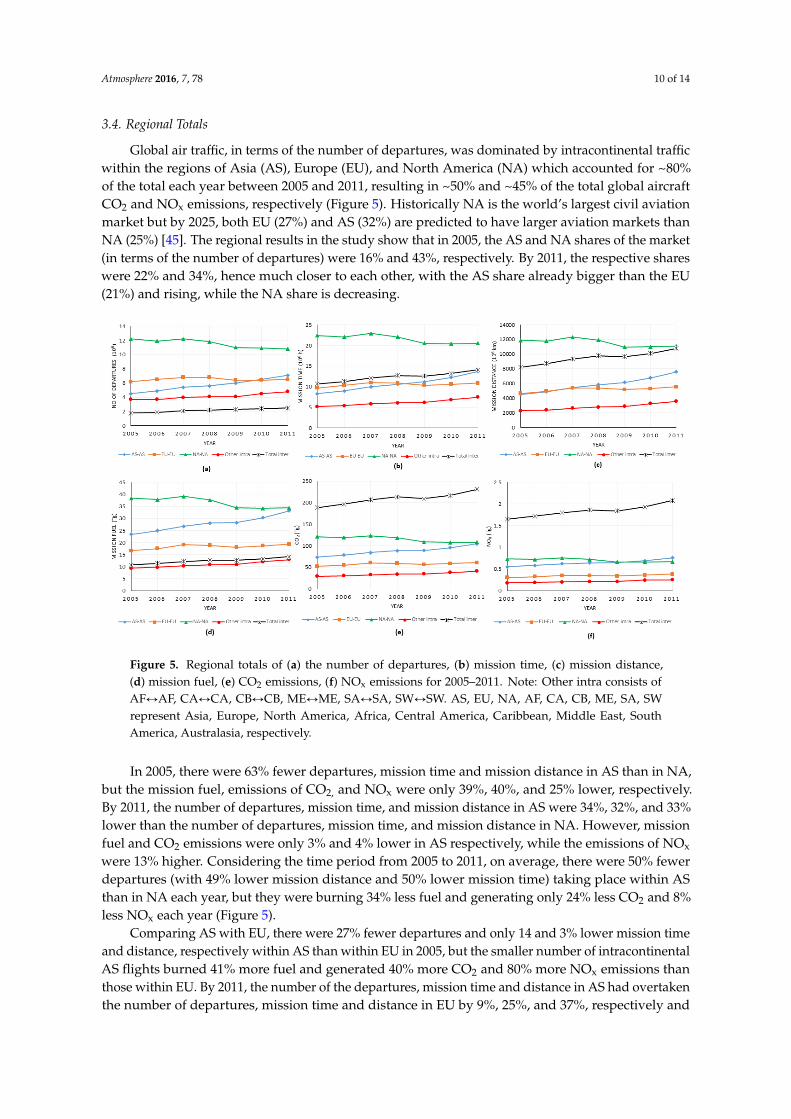
Figure 5. Regional totals of (a) the number of departures, (b) mission time, (c) mission distance,

(d) mission fuel, (e) CO2 emissions, (f) NOx emissions for 2005–2011. Note: Other intra consists of

AFAF, CACA, CBCB, MEME, SASA, SWSW. AS, EU, NA, AF, CA, CB, ME, SA, SW

represent Asia, Europe, North America, Africa, Central America, Caribbean, Middle East, South

America, Australasia, respectively.

In 2005, there were 63% fewer departures, mission time and mission distance in AS than in NA,

but the mission fuel, emissions of CO2, and NOx were only 39%, 40%, and 25% lower, respectively.

By 2011, the number of departures, mission time, and mission distance in AS were 34%, 32%, and

33% lower than the number of departures, mission time, and mission distance in NA. However,

mission fuel and CO2 emissions were only 3% and 4% lower in AS respectively, while the emissions

of NOx were 13% higher. Considering the time period from 2005 to 2011, on average, there were 50%

fewer departures (with 49% lower mission distance and 50% lower mission time) taking place within

AS than in NA each year, but they were burning 34% less fuel and generating only 24% less CO2 and

8% less NOx each year (Figure 5).

Comparing AS with EU, there were 27% fewer departures and only 14 and 3% lower mission

time and distance, respectively within AS than within EU in 2005, but the smaller number of

intracontinental AS flights burned 41% more fuel and generated 40% more CO2 and 80% more NOx

emissions than those within EU. By 2011, the number of the departures, mission time and distance in

AS had overtaken the number of departures, mission time and distance in EU by 9%, 25%, and 37%,

Figure 5. Regional totals of (a) the number of departures, (b) mission time, (c) mission distance,(d) mission fuel, (e) CO2 emissions, (f) NOx emissions for 2005–2011. Note: Other intra consists ofAFØAF, CAØCA, CBØCB, MEØME, SAØSA, SWØSW. AS, EU, NA, AF, CA, CB, ME, SA, SWrepresent Asia, Europe, North America, Africa, Central America, Caribbean, Middle East, SouthAmerica, Australasia, respectively.

In 2005, there were 63% fewer departures, mission time and mission distance in AS than in NA,but the mission fuel, emissions of CO2, and NOx were only 39%, 40%, and 25% lower, respectively.By 2011, the number of departures, mission time, and mission distance in AS were 34%, 32%, and 33%lower than the number of departures, mission time, and mission distance in NA. However, missionfuel and CO2 emissions were only 3% and 4% lower in AS respectively, while the emissions of NOx

were 13% higher. Considering the time period from 2005 to 2011, on average, there were 50% fewerdepartures (with 49% lower mission distance and 50% lower mission time) taking place within ASthan in NA each year, but they were burning 34% less fuel and generating only 24% less CO2 and 8%less NOx each year (Figure 5).

Comparing AS with EU, there were 27% fewer departures and only 14 and 3% lower mission timeand distance, respectively within AS than within EU in 2005, but the smaller number of intracontinentalAS flights burned 41% more fuel and generated 40% more CO2 and 80% more NOx emissions thanthose within EU. By 2011, the number of the departures, mission time and distance in AS had overtakenthe number of departures, mission time and distance in EU by 9%, 25%, and 37%, respectively and

Atmosphere 2016, 7, 78 11 of 14

AS air traffic was generating 72% more CO2 emissions and 100% more NOx emissions by burning72% more fuel than EU air traffic. On average for the time period of 2005-2011, there were 12% fewerdepartures, but 2% increased mission time and 13% increased mission distance within AS than withinthe EU each year, however they were generating 52% and 87% more CO2 and NOx per year (Figure 5).Comparing EU to NA, the results were more uniform. Between 2005 and 2011, on average, EU annualintracontinental departures, mission distance, mission time were 44%, 55%, and 51%, respectivelylower than NA, but the mission fuel, CO2, and NOx annual emissions were also 50% lower within theEU than within NA (Figure 5).

The variabilities in the regional emission intensities of CO2 between AS, EU, NA during thetime period of 2005–2011 suggest that AS air traffic is contributing more to aviation’s fraction ofthe total global CO2 burden. The regional and global atmospheric impact of the differences in theregional emissions intensities of aircraft NOx, in terms of increased tropospheric O3 production,is heterogeneous. Gilmore et al. [46] showed that the magnitude of sensitivity for southeast AS is afactor of 2 higher relative to NA for global O3 due to changes in regional NOx emissions. In this study,the annual average increase in the number of departures within AS was 8%, 1% in EU, and ´1.9% inNA. Aviation is growing significantly faster in AS compared with EU and NA, so the emissions ofNOx from aircraft grow at a higher rate and with a higher intensity in AS, which also has the strongestresponse in terms of O3 production to the addition of the NOx emissions.

4. Conclusions

On the 20th anniversary of the first comprehensive aircraft emission inventory, we presenteda timeline of seven consecutive years (2005–2011) of estimates of the mission fuel burn, a reservefuel requirement, and the emissions of CO2, CO, H2O, HC, NOx, and SOx of present day global andregional air traffic. The estimation referred to as the 4-D Aircraft Fuel Burn and Emissions Inventorywas based on a detailed representation of the global fleet derived from actual records of air trafficmovements and a detailed distribution of the fuel consumption and the emissions throughout theentire flight cycle. The 4-D Aircraft Fuel Burn and Emissions Inventory enabled a consistent globaland regional trend analysis (2005–2011) and comparison of fuel burn and emissions for the first timesince Kim et al. [27] who presented estimates for the time period 2000–2005, thus picking up thetimeline in 2005, extending it to 2011, and bringing it up-to-date. An estimate of a global reservefuel requirement was given for the first time within this work, which together with the mission fuelburn estimate provides an improved quantification of the global aviation fuel consumption with afuel match of 1.1 (a 10% overestimate) relative to an IEA estimate for the total global jet keroseneproduction for 2009. The inventory results revealed that global estimates mask substantial regionalfluctuations and differences in the quantity and distribution of the aircraft NOx emissions and in thenumber of departures, in particular, a persistent decline in North America and persistent growthin Asia. Moreover, a trend of substantially higher CO2 and NOx emission intensities within Asia isfound if we compare their emissions within Europe and North America. A gradual shift in the globaldistribution of the NOx emissions from aircraft, and a subtle but steady change in the regional emissiontrends, are found with comparatively higher and rising growth rates in latitudes 0–30˝N. These factorsmay have potentially large atmospheric implications in light of recent findings which indicate that thesensitivities to aircraft NOx emissions in Southeast Asia are more than double those in North Americaand Europe [46].

Supplementary Materials: The following are available online at http://www.mdpi.com/2073-4433/7/6/78/s1,Figure S1: Vertical distribution of the global aircraft CO2 emissions during 2005–2011; Figure S2: Verticaldistribution of the global aircraft H2O emissions during 2005–2011; Figure S3: Vertical distribution of the globalaircraft SOx emissions during 2005–2011.

Acknowledgments: We thank Stephen Roome (University of Bristol, IT support), Tom Gidden (http://www.linkedin.com/in/tomgidden), Matt Oates (University of Bristol, Bristol Centre for Complexity Sciences),Callum Wright (University of Bristol, Advanced Computing Research Centre), Sergio Angel Araujo Estrada(University of Bristol, Department of Aerospace Engineering), and Andy Williams for their support during the

Atmosphere 2016, 7, 78 12 of 14

work. We also thank the Engineering and Physical Sciences Research Council (EPSRC) (grant EP/5011214) andthe Natural Environmental Research Council (NERC) (grant-NE/J009008/1 and NE/I014381/1), University ofBristol Faculty of Engineering and School of Chemistry for funding various aspects of this work.

Author Contributions: D.K. Wasiuk, D.E. Shallcross, and M.H. Lowenberg conceived the idea, designed theexperiments; D.K. Wasiuk and M.A.H. Khan analysed the data and wrote the paper; M.H. Lowenberg andD.E. Shallcross provided important suggestions and approved the final manuscript.

Conflicts of Interest: The authors declare no conflict of interest.

References

1. Penner, J.E.; Lister, D.H.; Griggs, D.J.; Dokken, D.J.; McFarland, M. Aviation and the Global Atmosphere.A Special Report of Working Groups I and III of the Intergovernmental Panel on Climate Change (IPCC); CambridgeUniversity Press: Cambridge, UK, 1999.

2. Lee, D.S.; Pitari, G.; Grewe, V.; Gierens, K.; Penner, J.E.; Petzold, A.; Prather, M.J.; Schumann, U.; Bais, A.;Berntsen, T.; et al. Transport impacts on atmosphere and climate: Aviation. Atmos. Environ. 2010, 44,4678–4734. [CrossRef]

3. Lee, D.S.; Fahey, D.W.; Forster, P.M.; Newton, P.J.; Wit, R.C.N.; Lim, L.L.; Owen, B.; Sausen, R. Aviation andglobal climate change in the 21st century. Atmos. Environ. 2009, 43, 3520–3537. [CrossRef]

4. Mahashabde, A.; Wolfe, P.; Ashok, A.; Dorbian, C.; He, Q.; Fan, A.; Lukachko, S.; Mozdzanowska, A.;Wollersheim, C.; Barrett, S.R.H.; et al. Assessing the environmental impacts of aircraft noise and emissions.Prog. Aero. Sci. 2011, 47, 15–52. [CrossRef]

5. Holmes, C.D.; Tang, Q.; Prather, M.J. Uncertainties in climate assessment for the case of aviation NO.Proc. Natl Acad. Sci. USA 2011, 108, 10997–11002. [CrossRef] [PubMed]

6. Burkhardt, U.; Kärcher, B. Global radiation forcing from contrail cirrus. Nat. Clim. Change 2011, 1, 54–58.[CrossRef]

7. Skowron, A.; Lee, D.S.; de León, R.R. The assessment of the impact of aviation NOx on ozone and otherradiative forcing responses: The importance of representing cruise altitudes accurately. Atmos. Environ. 2013,74, 159–168. [CrossRef]

8. Olsen, S.C.; Wuebbles, D.J.; Owen, B. Comparison of global 3-D aviation emissions datasets.Atmos. Chem. Phys. 2013, 13, 429–441. [CrossRef]

9. Dessens, O.; Köhler, M.O.; Rogers, H.L.; Jones, R.L.; Pyle, J.A. Aviation and climate change. Transport. Policy2014, 34, 14–20. [CrossRef]

10. Brasseur, G.P.; Gupta, M.; Anderson, B.E.; Balasubramanian, S.; Barrett, S.; Duda, D.; Fleming, G.;Forster, P.M.; Fuglestvedt, J.; Gettelman, A.; et al. Impact of Aviation on Climate: FAA’s Aviation ClimateChange Research Initiative (ACCRI) Phase II. Bull. Amer. Meteor. Soc. 2015. [CrossRef]

11. Airbus. Global Market Forecast 2015–2034, 2015. Available online: http://www.airbus.com/company/market/forecast/ (accessed on 20 December 2015).

12. European Commission Climate Action (ECCA), 2015. Available online: http://ec.europa.eu/clima/policies/transport/aviation/index_en.htm (accessed on 21 August 2015).

13. Brasseur, G.P.; Cox, R.A.; Hauglustaine, D.; Isaksen, I.; Lelieveld, J.; Lister, D.H.; Sausen, R.; Schumann, U.;Wahner, A.; Wiesen, P. European scientific assessment of the atmospheric effects of aircraft emissions.Atmos. Environ. 1998, 32, 2329–2418. [CrossRef]

14. Kentarchos, A.S.; Roelofs, G.J. Impact of aircraft NOx emissions on tropospheric ozone calculated with achemistry general circulation model: sensitivity to higher hydrocarbon chemistry. J. Geophys. Res. 2002, 107,ACH 8-1–ACH 8-12. [CrossRef]

15. Brühl, C.; Pöschl, U.; Crulzen, P.J.; Steil, B. Acetone and PAN in the upper troposphere: Impact on ozoneproduction from aircraft emissions. Atmos. Environ. 2000, 34, 3931–3938. [CrossRef]

16. Köhler, M.O.; Rädel, G.; Dessens, O.; Shine, K.P.; Rogers, H.L.; Wild, O.; Pyle, J.A. Impact of perturbations tonitrogen oxide emissions from global aviation. J. Geophys. Res. 2008, 113, D11305. [CrossRef]

17. Grewe, V.; Stenke, A. AirClim: An efficient tool for climate evaluation of aircraft technology.Atmos. Chem. Phys. 2008, 8, 4621–4639. [CrossRef]

18. Pitari, G.; Mancini, E.; Bregman, A. Climate forcing of subsonic aviation: Indirect role of sulfate particles viaheterogeneous chemistry. Geophys. Res. Lett. 2002, 29, 2057. [CrossRef]

Atmosphere 2016, 7, 78 13 of 14

19. McInnes, G.; Walker, C.T. The Global Distribution of Aircraft Air Pollutant Emissions; Warren Spring LaboratoryReport LR872; Department of Trade and Industry, Warren Spring Laboratory: Stevenage, UK, 1992.

20. Wuebbles, D.J.; Maiden, D.; Seals, R.K.; Baughcum, S.L.; Metwally, M.; Mortlock, A. Emissions scenariosdevelopment: Report of the emissions scenarios committee. In The Atmospheric Effects of Stratospheric Aircraft:A Third Program Report; NASA Reference Publication 1313; Stolarski, R.S., Wesoky, H.L., Eds.; NationalAeronautics and Space Administration: Washington, DC, USA, 1993; pp. 63–85.

21. ANCAT/EC. A Global Inventory of Aircraft NOx Emissions. A First Version (April 1994) Prepared for theAERONOX Programme; Abatement of Nuisances Caused by Air Transport (ANCAT) and EuropeanCommunity Working Group: London, UK, 1995.

22. Baughcum, S.L.; Henderson, S.C.; Hertel, P.S.; Maggiora, D.R.; Oncina, C.A. Stratospheric Emissions EffectsDatabase Development; Boeing Commercial Airplane Group, National Aeronautics and Space Administration(NASA) Contractor Report 4592; Langley Research Centre: Hampton, VA, USA, 1994.

23. Baughcum, S.L.; Henderson, S.C.; Tritz, T.G. Scheduled Civil Aircraft Emission Inventories for 1976 and 1984:Database Development and Analysis; Boeing Commercial Airplane Group, National Aeronautics and SpaceAdministration (NASA) Contractor Report-4722; Langley Research Centre: Hampton, VA, USA, 1996.

24. Baughcum, S.L.; Tritz, T.G.; Henderson, S.C.; Pickett, D.C. Scheduled Civil Aircraft Emission Inventories for 1992:Database Development and Analysis; National Aeronautics and Space Administration Contractor Report-4700;Langley Research Centre: Hampton, VA, USA, 1996.

25. Sutkus, D.J., Jr.; Baughcum, S.L.; DuBois, D.P. Commercial Aircraft Emission Scenario for 2020: DatabaseDevelopment and Analysis; NASA/CR-2003-212331; National Aeronautics and Space Administration, GlennResearch Centre: Hanover, MD, USA, 2003.

26. Eyers, C.J.; Norman, P.; Middel, J.; Plohr, M.; Michot, S.; Atkinson, K. AERO2k Global Aviation EmissionsInventories for 2002 and 2025; European Commission, QinetiQ Ltd.: Hampshire, UK, 2004.

27. Gardner, R.M.; Adams, K.; Cook, T.; Deidewig, F.; Ernedal, S.; Falk, R.; Fleuti, E.; Herms, E.; Johnson, C.E.;Lecht, M.; et al. The ANCAT/EC global inventory of NOx emissions from aircraft. Atmos. Environ. 1997, 31,1751–1766. [CrossRef]

28. Kim, B.Y.; Fleming, G.; Balasubramanian, S.; Malwitz, A.; Lee, J.; Waitz, I.; Klima, K.; Locke, M.; Holsclaw, C.;Morales, A.; McQueen, E.; Gillette, W. System for Assessing Aviation’s Global Emissions (SAGE), Version 1.5;Global Aviation Emissions Inventories for 2000 through 2004; FAA-EE-2005–02; Federal Aviation AdministrationOffice of Environment and Energy: Washington, DC, USA, 2005.

29. Kim, B.Y.; Fleming, G.G.; Lee, J.J.; Waitz, I.A.; Clarke, J.P.; Balasubramanian, S.; Malwitz, A.; Klima, K.;Locke, M.; Holslaw, C.A.; et al. System for assessing Aviation’s Global Emissions (SAGE), Part 1: Modeldescription and inventory results. Transport. Res. Part D: Transp. Environ. 2007, 12, 325–346. [CrossRef]

30. Wilkerson, J.T.; Jacobson, M.Z.; Malwitz, A.; Balasubramanian, S.; Wayson, R.; Fleming, G.; Naiman, A.D.;Lele, S.K. Analysis of emission data from global commercial aviation: 2004 and 2006. Atmos. Chem. Phys.2010, 10, 6391–6408. [CrossRef]

31. Owen, B.; Lee, D.S.; Lim, L. Flying into the future: aviation emissions scenarios to 2050. Environ. Sci. Technol.2010, 44, 2255–2260. [CrossRef] [PubMed]

32. Chèze, B.; Gastineau, P.; Chevallier, J. Forecasting world and regional aviation jet fuel demands to themid-term (2025). Energy Policy 2011, 39, 5147–5158. [CrossRef]

33. Simone, N.W.; Stettler, M.E.J.; Barrett, S.R.H. Rapid estimation of global civil aviation emissions withuncertainty quantification. Transport. Res. Part D Transp. Environ. 2013, 25, 33–41. [CrossRef]

34. Yan, F.; Winijkul, E.; Streets, D.G.; Lu, Z.; Bond, T.C.; Zhang, Y. Global emission projections for thetransportation sector using dynamic technology modelling. Atmos. Chem. Phys. 2014, 14, 5709–5733.[CrossRef]

35. Wasiuk, D.K.; Lowenberg, M.H.; Shallcross, D.E. An aircraft performance model implementation for theestimation of global and regional commercial aviation fuel burn and emissions. Transport. Res. Part DTransp. Environ. 2015, 35, 142–159. [CrossRef]

36. ICAO. Aircraft Engine Emissions Databank, 18th ed.; International Civil Aviation Organization Committee onAviation Environmental Protection: Montreal, YQB, Canada, 2012.

37. Hasselrot, A. Confidential Database for Turboprop Engine Emissions; Swedish Defence Research Agency:Stockholm, Sweden, 2002.

Atmosphere 2016, 7, 78 14 of 14

38. DuBois, D.; Paynter, G.C. Fuel Flow Method 2 for Estimating Aircraft Emissions; SAElnternational, The BoingCompany: Washington, DC, USA, 2006.

39. SAE. SAE Aerospace. Procedure for the Calculation of Aircraft Emissions; Technical Report AIR5715;SAE International: Warrendale, PA, USA, 2009.

40. Collins, W.J.; Stevenson, D.S.; Johnson, C.E.; Derwent, R.G. Tropospheric ozone in a Global-ScaleThree-Dimensional Lagrangian Model and its response to NOx emission controls. J. Atmos. Chem. 1997, 26,223–274. [CrossRef]

41. Utembe, S.R.; Cooke, M.C.; Archibald, A.T.; Jenkin, M.E.; Derwent, R.G.; Shallcross, D.E. Using a reducedCommon Representative Intermediates (CRI v2-R5) mechanism to simulate tropospheric ozone in a 3-DLagrangian chemistry transport model. Atmos. Environ. 2010, 13, 1609–1622. [CrossRef]

42. Schumann, U. The impact of nitrogen oxides emissions from aircraft upon the atmosphere at flightaltitudes–results from the AERONOX project. Atmos. Environ. 1997, 31, 1723–1733. [CrossRef]

43. IEA. International Energy Agency Oil Statistics. 2015. Available online: http://www.iea.org/stats/oildata.asp?COUNTRY_CODE=29 (accessed on 06 May 2015).

44. Sutkus, D.J., Jr.; Baughcum, S.L.; DuBois, D.P. Scheduled Civil Aircraft Emission Inventories for 1999: DatabaseDevelopment and Analysis; NASA/CR-2001-211216; National Aeronautics and Space Administration, GlennResearch Centre: Hanover, MD, USA, 2001.

45. Belobaba, P.; Odoni, A.; Barnhart, C. The Global Airline Industry, 2nd ed.; John Wiley & Sons, Ltd.: West Sussex,UK, 2015.

46. Gilmore, C.K.; Barrett, S.R.H.; Koo, J.; Wang, Q. Temporal and spatial variability in the aviation NOx-relatedO3 impact. Environ. Res. Lett. 2013, 8, 034027. [CrossRef]

© 2016 by the authors; licensee MDPI, Basel, Switzerland. This article is an open accessarticle distributed under the terms and conditions of the Creative Commons Attribution(CC-BY) license (http://creativecommons.org/licenses/by/4.0/).