a

N A S A T E C H N I C A L R E P O R T

A COMBINED NEWTON-RAPHSON A N D GRADIENT PARAMETER CORRECTION TECHNIQUE FOR SOLUTION OF OPTIMAL-CONTROL PROBLEMS

by Ernest S. Armstrong

LungZey Resemch Center LungZey Stution, Humpton,

N A T I O N A L AERONAUTICS A N D SPACE

Vd.

R-293

A D M I N I S T R A T I O N WASHINGTON, D. C. OCTOBER 1 9 6 8

https://ntrs.nasa.gov/search.jsp?R=19680027601 2019-07-14T19:24:34+00:00Z

TECH LIBRARY KAFB, NM

I111111 lllll lllll111ll lllll lllll /Ill1 Ill1 1111

A COMBINED NEWTON-RAPHSON AND GRADIENT

P A R A M E T E R CORRECTION TECHNIQUE F O R SOLUTION

O F OPTIMAL-CONTROL PROBLEMS

/--

By E r n e s t S. A r m s t r o n g

Langley R e s e a r c h C e n t e r

Langley Station, Hanipton, Va.

r / /’ NATIONAL AERONAUTICS AND SPACE A D M , W A I I O N

For sale by the Clearinghouse for Federal Scientific and Technical Information Springfield, Virginia 22151 - CFSTI price $3.00

I

CONTENTS

Page SUMMARY . . . . . . . . . . . . . . . . . . . . . . . . . . . . . . . . . . . . . . . 1

INTRODUCTION . . . . . . . . . . . . . . . . . . . . . . . . . . . . . . . . . . . . 1

SYMBOLS . . . . . . . . . . . . . . . . . . . . . . . . . . . . . . . . . . . . . . . 3

PROBLEM STATEMENT . . . . . . . . . . . . . . . . . . . . . . . . . . . . . . . 10 Indirect Optimal-Control Theory . . . . . . . . . . . . . . . . . . . . . . . . . . 10

13

15 Iterative Logic . . . . . . . . . . . . . . . . . . . . . . . . . . . . . . . . . . . . 15 Convergence . . . . . . . . . . . . . . . . . . . . . . . . . . . . . . . . . . . . . 17 Relation to Gradient and Newton-Raphson Processes . . . . . . . . . . . . . . . 19

A Particular Boundary-Value Problem . . . . . . . . . . . . . . . . . . . . . . . THEORETICAL DEVELOPMENT OF CORRECTION TECHNIQUE . . . . . . . . . .

. . . . . . . . . . . . . . . . . . . . . . . . . . . . . . . . . 19

Critical Review . . . . . . . . . . . . . . . . . . . . . . . . . . . . . . . . . . . 27

EXAMPLE CALCULATION . . . . . . . . . . . . . . . . . . . . . . . . . . . . . . 28 Problem Statement . . . . . . . . . . . . . . . . . . . . . . . . . . . . . . . . . 28 Application of Algorithm . . . . . . . . . . . . . . . . . . . . . . . . . . . . . . 28 Results . . . . . . . . . . . . . . . . . . . . . . . . . . . . . . . . . . . . . . . . 36

CONCLUDING REMARKS . . . . . . . . . . . . . . . . . . . . . . . . . . . . . . . 41

APPENDIX A . PROOF OF LEMMAS USED TO ESTABLISH THEOREM 1 . . . . . 43 L e m m a 1 . . . . . . . . . . . . . . . . . . . . . . . . . . . . . . . . . . . . . . . 43 L e m m a 2 . . . . . . . . . . . . . . . . . . . . . . . . . . . . . . . . . . . . . . . 45 L e m m a 3 . . . . . . . . . . . . . . . . . . . . . . . . . . . . . . . . . . . . . . . 47

APPENDIX B . DYNAMIC EQUATIONS FOR LUNAR-RENDEZVOUS PROBLEM . . . . . . . . . . . . . . . . . . . . . . . . . . . . . . . . . . . . . . 48

APPENDIX C . NECESSARY CONDITIONS FOR FUEL-OPTIMAL RENDEZVOUS . . . . . . . . . . . . . . . . . . . . . . . . . . . . . . . . . . . . 56

REFERENCES . . . . . . . . . . . . . . . . . . . . . . . . . . . . . . . . . . . . . 61

iii

A COMBINED NEWTON-RAPHSON AND GRADIENT

PARAMETER CORRECTION TECHNIQUE FOR SOLUTION

OF OPTIMAL-CONTROL PROBLEMS*

By Ernest S. Armstrong Langley Research Center

SUMMARY

A parameter correction technique is developed to solve a boundary-value problem which frequently occurs in optimal-control theory. It is assumed that an indirect optimal-control method has been applied to a controllable dynamic system with a two- point boundary-value problem resulting such that the boundary conditions take the form of a set of unknown parameters to be determined to meet an equal number of terminal conditions. The optimal-control law is a piecewise continuous function with discontinu- ities occurring only at the zeros of certain continuous functions. A procedure is devel- oped to improve upon an assumed se t of parameters so that, by repetitive use of a cor- rection formula, a monotonic decreasing sequence of values of a positive definite function that measures the terminal e r r o r s is produced. The direction of the correction vector is found to lie between the directions given by the gradient and the Newton-Raphson procedures.

Integral equations are derived for influence matrices that describe the effect of a change in the parameters on the terminal conditions.

The procedure is successfully applied to the determination of both planar and non- planar fuel-optimal trajectories for a space vehicle which is launched from the surface of the moon and required to rendezvous with a space vehicle in a circular orbit.

INTRODUCTION

In recent years, control theory has been expanded to include the area of system optimization. This expansion has brought about a new design philosophy. Control

*This report is based in par t upon a thesis entitled "An Algorithm for the Iterative Solution of a Class of Two- Point Boundary-Value Problems Occurring in Optimal- Control Theory" offered in partial fulfillment of the requirements for the degree of Doctor of Philosophy in Mathematics, North Carolina State University of Raleigh, Raleigh, North Carolina, June 19 67.

functions may now be chosen to optimize in some given sense the system response to the control action; for example, a control law may be found to force a system to a given state while some functional of the system variables is minimized. This new a rea of research is termed optimal-control theory.

Present-day methods of calculating optimal- control solutions can be grouped into two classes: direct and indirect. Both methods a r e designed to minimize the value of some functional. A direct method depends upon a comparison of the values of the func- tional at two or more points. An indirect method is used to find a solution by means of necessary (and sometimes sufficient) conditions for a minimum. a r e contained in references 1 to 3. Necessary conditions to be used in an indirect approach are found by applying the Pontryagin maximum principle (ref. 4), or the calculus of variations (ref. 5), or dynamic programing (ref. 6). In general, the necessary condi- tions take the form of a set of nonlinear differential equations with both initial and final boundary conditions; that is, in order to obtain explicit solutions, a nonlinear two-point boundary-value problem must be solved.

Typical direct methods

The advent of high- speed computers has made feasible the solution of optimization problems by the method of successive approximations. illustrated by the success of the aforementioned direct methods. In these methods, a control history is first assumed and then successively improved upon by the computation of time-dependent corrections arrived at through the use of gradient (refs. 1 and 2) or conjugate-gradient (ref. 3) theory in function space. Although many useful results have been obtained in this manner, direct methods, in general, do not guarantee that the solu- tions obtained satisfy the necessary conditions of the indirect theory.

This procedure is markedly

A more rigorous, but computationally more difficult, approach is the use of neces- In this way, sa ry conditions of the indirect theory for the generation of optimal results.

one of the theories of references 4, 5, or 6 is applied, and then an attempt is made to solve whatever boundary-value problem might ensue. This approach is adopted herein.

The purpose of this report is to present a successive approximation procedure for attacking a class of two-point boundary-value problems which frequently occurs in the application of indirect optimization theory. Basically, the boundary-value problem is one in which the optimal-control law is piecewise continuous and in which there a r e a number of system parameters to be determined to meet an equal number of terminal con- ditions. A parameter correction procedure is developed in which an assumed set of parameters can be improved upon s o that, by repetitive use of a correction formula, a monotonic decreasing sequence of values of a positive definite function that measures the terminal e r r o r s is produced. between the direction given by the gradient and the Newton-Raphson procedures (ref. 7).

The direction of the parameter correction vector l ies

2

Integral equations are derived, the solutions of which yield influence matrices that describe the effect of a change in the parameters on the terminal conditions.

In order to exemplify the usefulness of the procedure, the Pontryagin maximum principle is applied to determine planar and nonplanar fuel-optimal trajectories for a space vehicle.which is launched from the surface of the moon and required to rendezvous with a space station in a circular orbit. The technique is then successfully applied to solve the resulting two-point boundary-value problem.

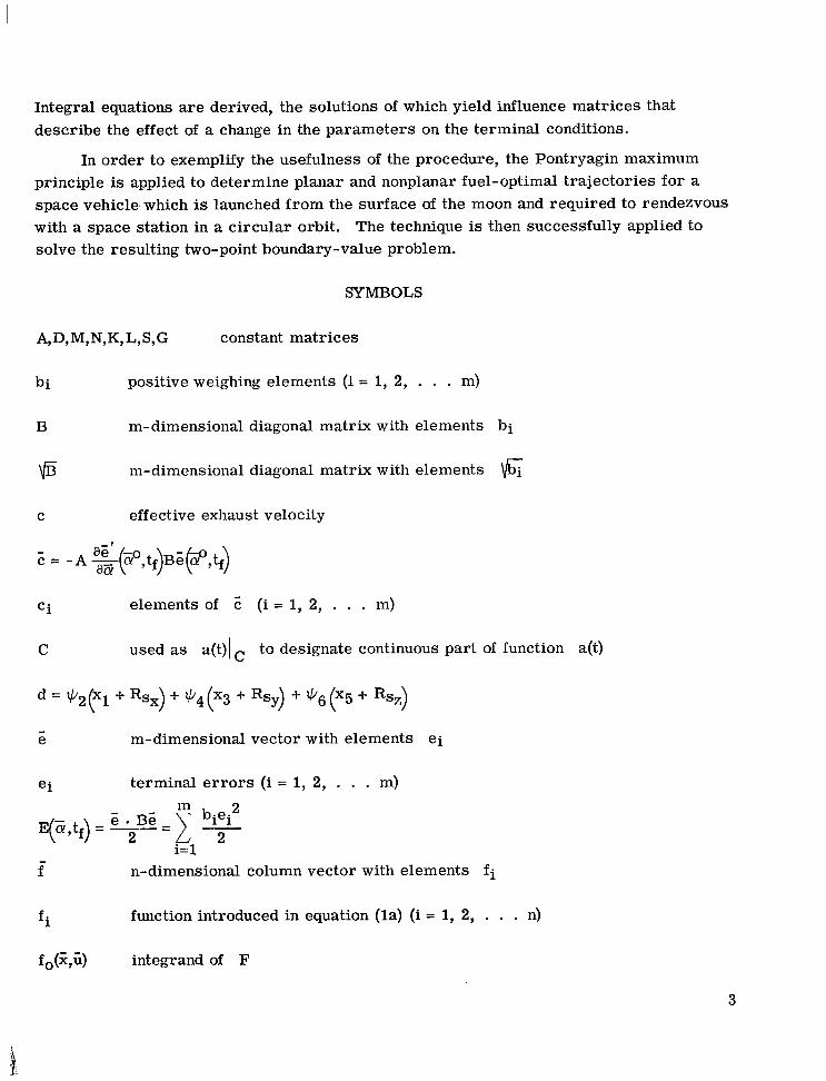
SYMBOLS

bi positive weighing elements (i = 1, 2, . . . m)

B m-dimensional diagonal matrix with elements bi

F m-dimensional diagonal matrix with elements 6 C effective exhaust velocity

C i elements of C (i = I, 2, . . . m)

C used as a(t)Ic to designate continuous part of function a(t)

- e m-dimensional vector with elements ei

ei terminal e r r o r s (i = 1, 2, . . . m)

- f n-dimensional column vector with elements f i

f i function introduced in equation (la) (i = 1, 2, . . . n)

f O ( G ) integrand of F

3

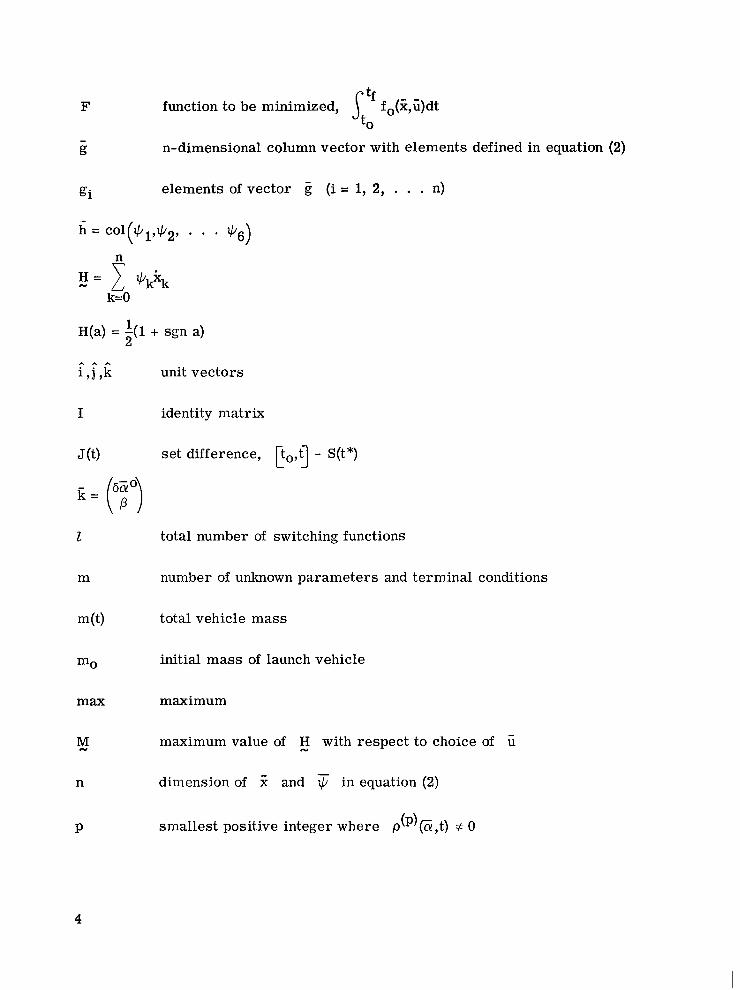
F function to be minimized, s' f0(%,6)dt t0

- g n-dimensional column vector with elements defined in equation (2)

elements of vector (i = 1, 2, . . . n) gi

H(a) = A(1 + sgn a)

i , j ,k unit vectors

2 _ . . A

I identity matrix

J (t) set difference, po,g - S(t9

1 total number of switching functions

m number of unknown parameters and terminal conditions

m (t) total vehicle mass

"0 initial mass of launch vehicle

max maximum

maximum value of H with respect to choice of fi M

M

n dimension of % and in equation (2)

M

P smallest positive integer where p(p)(Z,t) it 0

4

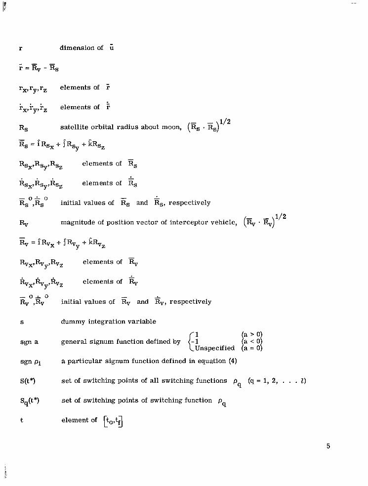
r dimension of u

rX,ry,rZ elements of 5

$x,%y,i-z elements of 5

RS

Rs = iRs, + fRSy + GRs,

Rsx9Rsy9Rsz elements of RS

Rs,,Rsy,Rs, elements of Rs

- 1/2 satellite orbital radius about moon, (Es * Rs)

-

- 0 - 0 Rs ,Rs initial values of Rs and E,, respectively

1/2 magnitude of position vector of interceptor vehicle, (% * &)

Rvx,%y’R,z elements of

%x,fby,%z elements of R, - 0- 0 Rv ,Rv initial values of Rv and Sv, respectively

S dum my integration variable

1 (a ’ 0)

(bnspecified 5 s g n a

sgn Pi

general signum function defined by

a particular signum function defined in equation (4)

set of switching points of all switching functions p (q = 1, 2, . . . I ) q s (t *I

q Sq(t*) set of switching points of switching function p

t element of po,tf3

5

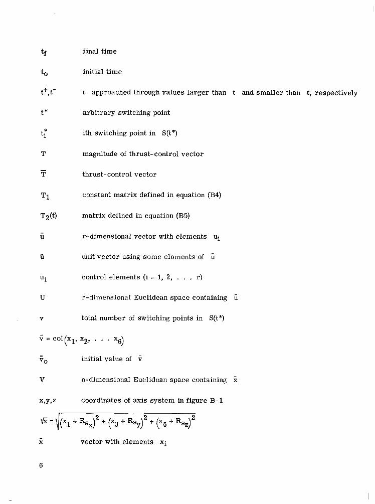
final time

initial time

t approached through values larger than t and smaller than t, respectively

arbitrary switching point

ith switching point in S ( t9

magnitude of thrust- control vector

thrust- control vector

constant matrix defined in equation (B4)

matrix defined in equation (B5)

r-dimensional vector with elements ui

unit vector using some elements of ii

control elements (i = 1, 2, . . . r)

r-dimensional Euclidean space containing U

total number of switching points in S(t*)

"6) v = col xl, x2, . . . - ( - VO initial value of ii

V n-dimensional Euclidean space containing x

X,Y,Z coordinates of axis system in figure B-1

- X vector with elements xi

6

xi state variables given by equation (la) (i = 1, 2, . . . n)

xo = kz fo(%,G)ds

coordinates of axis system in figure B-3

coordinates of axis system in figure B-3

equation (1 5) evaluated at (E ,tf)

vector defined in equation (B11)

m-dimensional vector with elements ai

unknown parameters ( i= 1, 2, . . . m)

vector defined in theorem 1 (i = 0, 1, . . .)

variable converting

largest allowable value of thrust magnitude

increment in a

increment in a! in gradient direction of -E(z,tf)

increment in 5 in Newton-Raphson direction

65. 6E 5 v2 into 6E * 6a! - v2 1- p2 = 0

AE(E,Q) = E(E+ 65,t.J - ~(5.9)

"E(G,Q) defined by equation (7)

- 5,; arbitrary m- dimens ional vectors

7

angles defined in figure B-2

angles defined in figure B-4

angles defined in figure B-3

Lagrange multiplier

value of X associated with v

ae ' ith eigenvalue of matrix :B 5 (i = 1, 2, . . . m) aa aa!

gravitational parameter of moon

bound on magnitude of 65

bound on magnitude of 6Zi

I-dimensional column vector of elements

switching function (i = 1, 2, . . . I )

arbitrary value of tc t tf

pi

coy 1 scalar function used as stopping condition

G vector with elements Qi (i = 1, 2, . . . n)

Il/i

@(Z,tf)

variables introduced by Pontryagin maximum principle (i = 0, 1, 2, . . . n)

equation (17) evaluated at (5,Q)

W angular velocity of moon about axis of rotation

- w = Ew

sz angular velocity of target in orbital plane

la1 absolute value of a

8

I

1 1 1 I1 I I I I I I I I I I I I I

- a designates a is vector

closed interval II.4 (a,b) open interval

w first derivative of a(t) with respect to t

a(t) second derivative of a(t) with respect to t

a(")(t), !.!%@

an) and 6 = col bl , . . . 5 * = f aibi if a = col al, , . .

nth derivative of a(t) with respect to t dtn

bn) ( ( i= 1

sum over all switching functions p (q = 1, 2, . . . Z) which have switching points at t*

Y q t * )

axi M x N Jacobian matrix with elements - where i = 1, 2, . . . M and a2 -

a? aY j

YN)

YN)

j = 1, 2, . . . N if 2 = col xl , . . . XM) and f = col yl , . , .

M X N matrix with elements - a a where i = 1, 2, . . . M and

xM) and 7 = col yl, . . . j = 1 , 2 , . . . N if % = c o l x l , . . .

(

(

2 (

2 a a q as 8x1 aYJ

( - 0 null vector

E belongs to a set

defined by A - -

A over a variable indicates a function of a! and t obtained by substitution for - %@,t) and qfi,t) into afunction of %fi,t), C/@,t), a, and t

N

?

over a variable indicates a function of t obtained by substitution for %@,t) - rc/@,t), and a! in afunction of x@,t), v@,t), 5, and t

over a matrix denotes matrix transpose

9

Subscripts :

j ,k, m,n,q, r,v,M,N

Superscripts:

i,P integers

integers

PROBLEM STATEMENT

Indirect Optimal- Control Theory

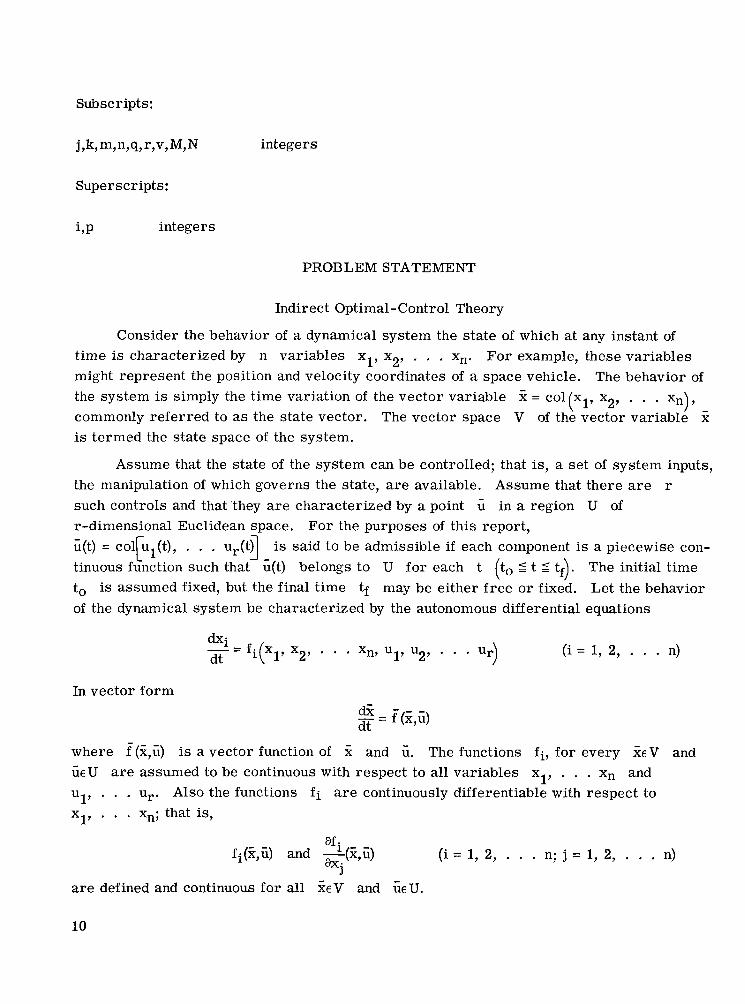
Consider the behavior of a dynamical system the state of which at any instant of t ime is characterized by n variables xl, x2, , , , Xn, For example, these variables might represent the position and velocity coordinates of a space vehicle. The behavior of the system is simply the t ime variation of the vector variable = col xl, x2, . . . Xn), commonly referred to as the state vector. The vector space V of the vector variable 2 is termed the state space of the system.

(

Assume that the state of the system can be controlled; that is, a set of system inputs, the manipulation of which governs the state, are available. Assume that there are r such controls and that’they a r e characterized by a point u in a region U of r-dimensional Euclidean space. u(t) = col ul(t), . . . ur(tg is said to be admissible if each component is a piecewise con- tinuous function such that ;(t) belongs to U for each t (to S t S Q). The initial time to is assumed fixed, but the final time tf may be either free o r fixed. Let the behavior of the dynamical system be characterized by the autonomous differential equations

For the purposes of this report, c

(i = 1, 2, . . . n) ki dt ( 1’ 2’ - = f i x x - Xn, ~ 1 , u2, . . .

In vector form & - dt - = f (2,ii)

where i(%,?i) is a vector function of % and 6. The functions f i , for every % V and UEU are assumed to be continuous with respect to all variables xl, . . . Xn and ul, . . . ur. Also the functions f i a r e continuously differentiable with respect to xl, . . , xn; that is,

a f i - - fi(2,;) and -(x,u) (i = 1, 2, . . . n; j = 1, 2, . , . n) axj

are defined and continuous for all ~ E V and &U.

10

.. . ...

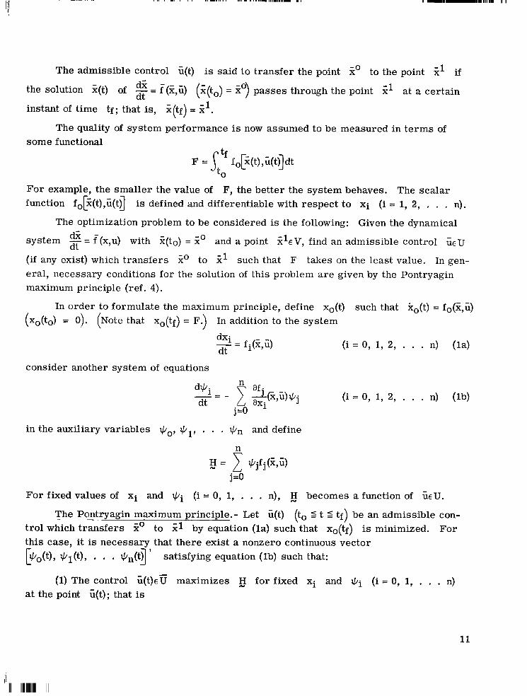
The admissible control u(t) is said to transfer the point xo to the point 2' if

the solution %(t) of - = i(%,i) (%(to) = zo) passes through the point %' at a certain dj; dt

instant of time tf; that is, %(tf) = x -1 . The quality of system performance is now assumed to be measured in t e rms of

some functional

F = L: fo[%(t),u(t)ldt

For example, the smaller the value of F, the better the system behaves. The scalar function fo[?(t),u(tg is defined and differentiable with respect to X i (i = 1, 2, . . . n).

The optimization problem to be considered is the following: Given the dynamical d% - dt system - = f (x,u) with :(to) = Zo and a point ?lev, find an admissible control UEU

(if any exist) which t ransfers go to 2' such that F takes on the least value. In gen- eral, necessary conditions for the solution of this problem a r e given by the Pontryagin maximum principle (ref. 4).

(xo(to) E 0). (Note that xo(tf) = F.) In addition to the system In order to formulate the maximum principle, define xo(t) such that xo(t) = fo(%,u)

dxi - - - fi(%,ii) dt

(i = 0, 1, 2, . . . n) (la)

consider another system of equations

af n d*i

dt 8x1 -= - 1 +F,ii)+j (i = 0, 1, 2, . . . n) (lb)

j =O

in the auxiliary variables qO7 +b17 . . . +n and define

n - €J = 1 +jfj(Z,G)

j =O

For fixedvalues of xi and qi (i = 0, 1, . . . n), g becomes afunction of &IT.

t rol which transfers Go to x1 by equation (la) such that xo(tf) is minimized. this case, it is necessary that there exist a nonzero continuous vector [,b0(t), Q1(t)? . . . +n(tj '

The Pontryagin - maximum principle.- Let u(t) (to 5 t 5 tf) be an admissible con- For

satisfying equation (lb) such that:

(1) The control U(t)Ec maximizes €J for fixed xi and +i (i = 0, 1, . . . n) at the point u(t); that is

11

( i=O, 1, . . . n; j = 1,2, . . . r) attained by substituting Then, $Jpi(t),xi(t)l represents the maximum value of

ii = U(t) into 5. (2) For all tePo,tf3, qo(t) = Constant 5 0 and gki(t) ,+i(tg = Constant = 0.

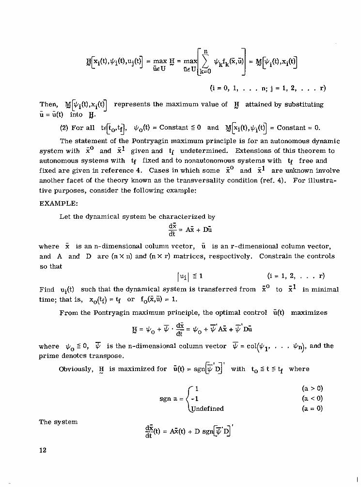
The statement of the Pontryagin maximum principle is for an autonomous dynamic system with and g1 given and tf undetermined. Extensions of this theorem to autonomous systems with tf fixed and to nonautonomous systems with tf f ree and fixed a r e given in reference 4. Cases in which some go and Z1 a r e unknown involve another facet of the theory known as the transversality condition (ref. 4). For illustra- tive purposes, consider the following example:

EXAMPLE:

Let the dynamical system be characterized by

where x is an n-dimensional column vector, u is an r-dimensional column vector, and A and D a r e (nX 11) and (nX r) matrices, respectively. Constrain the controls so that

Find time;

luil 5 1 (i = 1, 2, . . . r) ui(t) such that the dynamical system is transferred from go to 2' in minimal that is, xo(tf> = tf o r fo(z,i) = 1.

From the Pontryagin maximum principle, the optimal control u(t) maximizes

( -

where qo 5 0, prime denotes transpose.

is the n-dimensional column vector = col ql, . . . qn), and the

Obviously, H - is maximized for i(t) = sgnF'D]' with to 2 t S tf where

sgn a =

The system

12

I

1 _

... . ._ . . . . . - - ._ -. . .

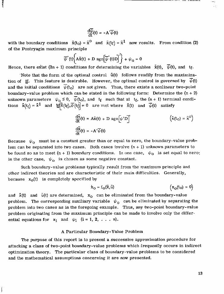
g ( t ) = -A'F(t)

with the boundary conditions ;;(to) = Z0 and Z(tf) = Z1 now results. From condition (2) of the Pontryagin maximum principle

Hence, there ezist (2n + 1) conditions for determining the variables :(t), F(t), and tf.

'Note that the form of the optimal control u(t) follows readily from the maximiza- tion of IJ. This feature is desirable. However, the optimal control is governed by F(t) and the initial conditions ?(to) a r e not given. Thus, there exists a nonlinear two-point boundary-value problem which can be stated in the following form: Determine the (n + 2) unknown parameters q0 9 0, +(to), and such that at tf, the (n + 1) terminal condi- tions ?(Q) = G1 and *(tf),?(tf] = 0 a r e met where Z(t) and T(t) satisfy

-

(?(to) = 2")

g ( t ) dt = -A'q(t)

Because Go must be a constant greater than or equal to zero, the boundary-value prob- lem can be separated into two cases. be found so as to meet (n + 1) boundary conditions. in the other case, Go is chosen as some negative constant.

Both cases involve (n + 1) unknown parameters to In one case, qo is set equal to zero;

Such boundary-value problems typically result from the maximum principle and other indirect theories and are characteristic of their main difficulties. because xo(t) is completely specified by

Generally,

ko = fo(G7i) (Xo(t0) = 0)

and z(t) and u(t) are determined, xo can be eliminated from the boundary-value problem. The corresponding auxiliary variable problem into two cases as in the foregoing example. problem originating from the maximum principle can be made to involve only the differ- ential equations for xi and +i (i = 1, 2, . . . n).

can be eliminated by separating the Thus, any two-point boundary-value

A Particular Boundary-Value Problem

The purpose of this report is to present a successive approximation procedure for attacking a class of two-point boundary-value problems which frequently occurs in indirect optimization theory. The particular class of boundary-value problems to be considered and the mathematical assumptions concerning it a r e now presented.

13

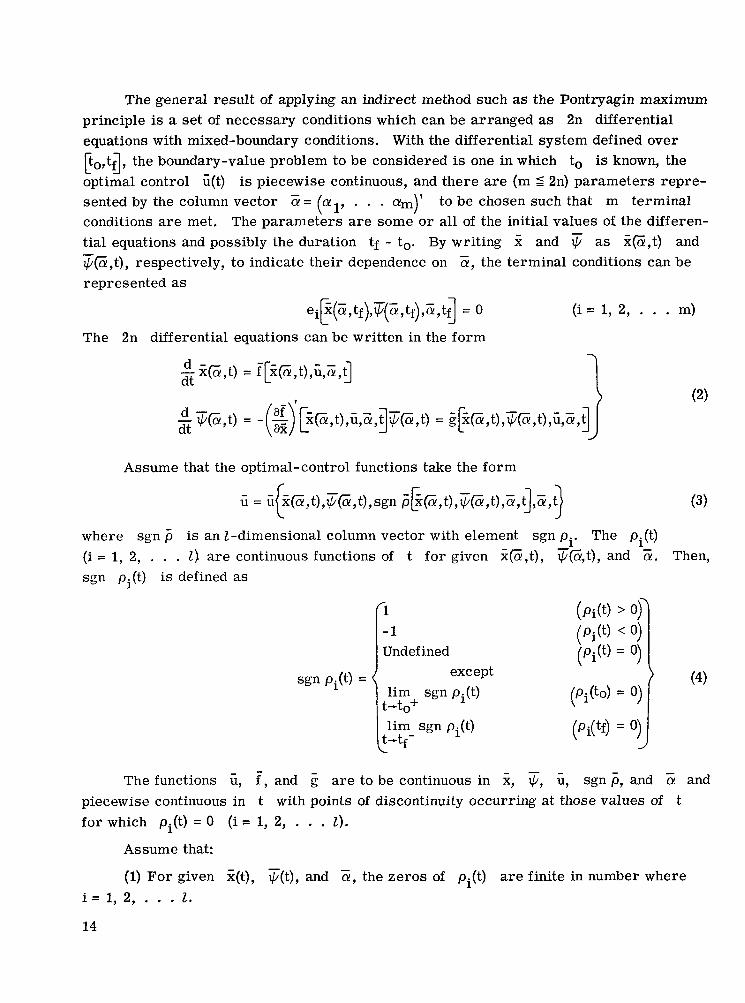
The general result of applying an indirect method such as the Pontryagin maximum principle is a set of necessary conditions which can be arranged as 2n differential equations with mixed-boundary conditions. With the differential system defined over p0,tf3, the boundary-value problem to be considered is one in which to is known, the optimal control u(t) is piecewise continuous, and there are (m S 2n) parameters repre- sented by the column vector E = al, . . . am)' to be chosen such that m terminal conditions a r e met. The parameters a r e some or all of the initial values of the differen- tial equations and possibly the duration tf - t,. By writing % and IF/ as %@,t) and +@,t), respectively, to indicate their dependence on a, the terminal conditions can be represented as

(

- -

eip(5 7tf),~(z 7 t f ) 9~ 7 t 4 = 0 (i = 1, 2, . . . m)

The 2n differential equations can be written in the form

- d %@,t) = f[2(Z,t),u,cY7g dt 7

Assume that the optimal-control functions take the form

where sgn 6 is an I-dimensional column vector with element sgn pi. The pi(t) (i = 1, 2, . . . I ) a r e continuous functions of t for given x@,t), TGt), and E . Then, sgn p. (t) is defined as

1

sgn Pi&) = lim sgn pi(t)

t-to+ lim sgn pi(t)

t-tf- c

(4)

- - - The functions 6, f , and E are to be continuous in x, +, u, sgn p , and a! and

piecewise continuous in t with points of discontinuity occurring at those values of t for which pi(t) = 0 (i = 1, 2, . . . I).

Assume that:

(1) For given %(t), IF/(t), and a, the zeros of pi(t) a r e finite in number where i = l , 2 , . . . 1.

14

1111 II 1111II II

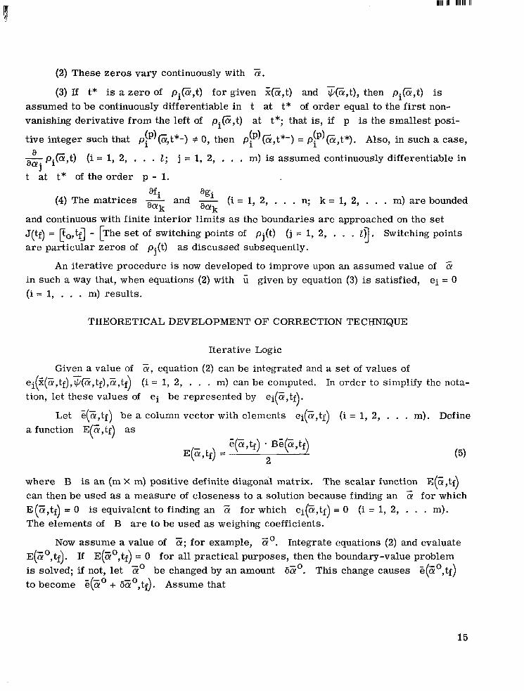
(2) These zeros vary continuously with Cy.

(3) If t* is a z e r o of pi@,t) for given g@,t) and ?@,t), then pi@,t) is assumed to be continuously differentiable in t at t* of order equal to the first non- vanishing derivative from the left of pi@,t) at t*; that is, if p is the smallest posi- tive integer such that pi (PI Et*- ) f 0, then pp)@,t*-) = pi (PI @,t*). Also, in such a case,

1, 2, . . . m) is assumed continuously differentiable in F p i @ , t ) a (i = 1, 2, . . . I ; j =

t at t* of the order p - 1.

afi 'gi (4) The matrices - and - (i = 1, 2, . . . n; k = 1, 2, . . . m) are bounded

aQ!k 'ak and continuous with finite interior limits as the boundaries a r e approached on the set J(tf) = pO,b] - [The set of switching points of pj(t) ( j = 1, 2, . . . 1'3. Switching points a r e particular zeros of p.(t) as discussed subsequently.

An iterative procedure is now developed to improve upon an assumed value of 5 in such a way that, when equations (2) with < given by equation (3) is satisfied, (i = 1, . . . m) results.

J

e i = 0

THEORETICAL DEVELOPMENT OF CORRECTION TECHNIQUE

Iterative Logic

ei(@,tf),G@,tf),Z,tf) (i = 1, 2, . . . m) can be computed. In order to simplify the nota- tion, let these values of e i be represented by ei(E,tf).

Let g(E,tf) be a column vector with elements ei(E,tf) (i = 1, 2, . . . m). Define a function E(5,tf) as

Given a value of 5 , equation (2) can be integrated and a set of values of

where B is an (m X m) positive definite diagonal matrix. can then be used as a measure of closeness to a solution because finding an a! for which E(5,tf) = 0 is equivalent to finding an Q! for which ei(Cy,tf) = 0 (i = 1, 2, . . . m). The elements of B a r e to be used as weighing coefficients.

The scalar function E(5,t.f) - -

Now assume a value of E ; for example, Eo. Integrate equations (2) and evaluate E(Eo,tf). If E(Zo,tf) = 0 for all practical purposes, then the boundary-value problem is solved; if not, let Eo be changed by an amount 65'. This change causes G(Eo,tf) to become .(Eo + 6Eo,tf). Assume that

15

I lllll 11l111l1ll1l111l111111111l

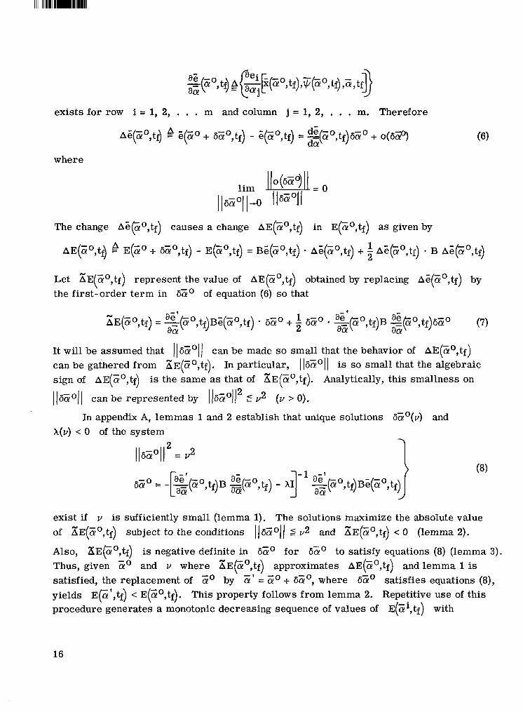
exists for row i = 1, 2, . . . m and column j = 1, 2, . . . m. Therefore

where

The change A6F0 , t f ) causes a change AE(Eo,tf) in E(zo,tf) as given by

E(zo + 6E0,tf) - E(zo,tf) = Be(Eo,tf) * Ae(E",tf) + AE(Eo,tf) Ae(Go,tf) - B AE(E0,tf)

Let xEIEo,tf) represent the value of AE(Eo,tf) obtained by replacing Ae(Zo,tf) by the first-order te rm in 6E0 of equation (6) so that

It will be assumed that I16EoII can be made so small that the behavior of AE(Eo,tf) can be gathered from aE(Eo,tf). In particular, 116E011 is so small that the algebraic sign of AE(z0,tf) is the same as that of aE(Eo,tf). Analytically, this smallness on

I/6E01) can be represented by ((60 11 5 v 2 (v > 0). " --O

In appendix A, lemmas 1 and 2 establish that unique solutions 6Zo(v) and X(v) < 0 of the system

(8)

1 ( 6 E O ( ) 2 2 = v

6Eo = -[g(Go,tf)B

exist if v is sufficiently small (lemma 1). The solutions maximize the absolute value of xE(zo,tf) subject to the conditions IISZoll 2 v2 and XE(Zo,tf) < 0 (lemma 2).

Also, KEFo,tf) is negative definite in SEo for sao to satisfy equations (8) (lemma 3). Thus, given E o and v where a E p o , t f ) approximates AE(Eo,tf) and lemma 1 is satisfied, the replacement of 6' by Z ' = ao + 6zo, where 6Eo satisfies equations (8), yields E(G',Q) < E(Zo,tf). This property follows from lemma 2. Repetitive use of this procedure generates a monotonic decreasing sequence of values of E(;Ei,tf) with

-

16

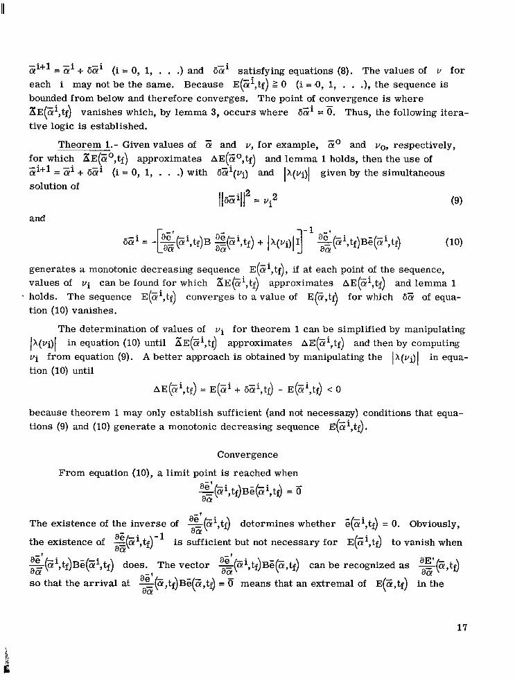
(i = 0, 1, . . .) and S z i satisfying equations (8). The values of v f o r zi+l= zi + Szi each i may not be the same. Because E(Zi,tf) 2 0 (i = 0, 1, . . .)7 the sequence is bounded from below and therefore converges. The point of convergence is where EE(zi,tf) vanishes which, by lemma 3, occurs where SZi = 0. Thus, the following itera- tive logic is established.

fo r which $E(Eo,tf) approximates AE(zo7tf) and lemma 1 holds, then the use of Zi+' = zi + SZi (i = 0, 1, . . .) with SZi(Vi) and IX(Ui)I

-

Theorem 1.- Givenvalues of a! and v, fo r example, Zo and vo, respectively,

given by the simultaneous solution of

IlSZill 2 2 = v i

and

(9)

generates a monotonic decreasing sequence E(Zi,tf), if at each point of the sequence, values of v i can be found for which aE(Zi,tf) approximates AE(Zi,tf) and lemma 1

- holds. The sequence E(Zi,tf) converges to a value of Ep , t f ) for which Sa! of equa- tion (10) vanishes.

The determination of values of v i for theorem 1 can be simplified by manipulating

IA(vi)l v i from equation (9). A better approach is obtained by manipulating the l A ( V i ) I in equa- tion (10) until

AE(Zi,tf) = E(Gi + SZi,tf) - E(zi,tf) < 0

in equation (10) until xE(Zi,tf) approximates AE(Ei,tf) and then by computing

because theorem 1 may only establish sufficient (and not necessavy) conditions that equa- tions (9) and (10) generate a monotonic decreasing sequence E(zi,tf).

Convergence

From equation (lo), a limit point is reached when

~ ( 6 ! i , t f ) B ~ ( z i , t ~ = 5 a a

The existence of the inverse of gPi,tf) determines whether G(Zi,tf) = 0. Obviously,

the existence of z(Zi,tf)-' is sufficient but not necessary for E(Zi,tf) to vanish when a a

- 1 a a

g(Zi,tf)BG(Zi,tf) does. The vector %(Ci,tf)Be(Z,tf) can be recognized as y ( a , t f ) aE' - aac - v a a a a - so that the arrival at $(E,tf)BE(Z,tf) = 0 means that an extremal of E(Z,tf) in the

a a

17

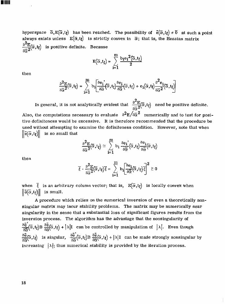
hyperspace E,E(Z,tf) has been reached. The possibility of e(E,tf) f b at such a point always exists unless E(E,tf) is strictly convex in 5; that is, the Hessian matrix - a" a,tf is positive definite. Because a,zT 1

i= 1 then

In general, 2

it is not analytically evident that 3 7 5 , t f ) need be positive definite. -.

Also, the computations necessary to evaluate numerically and to test for posi- tive definiteness would be excessive. It is therefore recommended that the procedure be used without attempting to examine the definiteness condition. llz(E,tf)l( is so small that

However, note that when

then

when IlS(E,tf)ll is small.

singular matrix may incur stability problems. The matrix may be numerically near singularity in the sense that a substantial loss of significant figures results from the inversion process. The algorithm has the advantage that the nonsingularity of

%Z,tf)B &,tf) + 1 XI1 can be controlled by manipulation of I XI. Even though a a =@,tf) a5 is singular, &,tf)B a:' =@,tf) a: + 1x11 can be made strongly nonsingular by aa increasing I X 1; thus numerical stability is provided by the iteration process.

is an arbitrary column vector; that is, E(E,tf) is locally convex when

A procedure which relies on the numerical inversion of even a theoretically non-

18

I

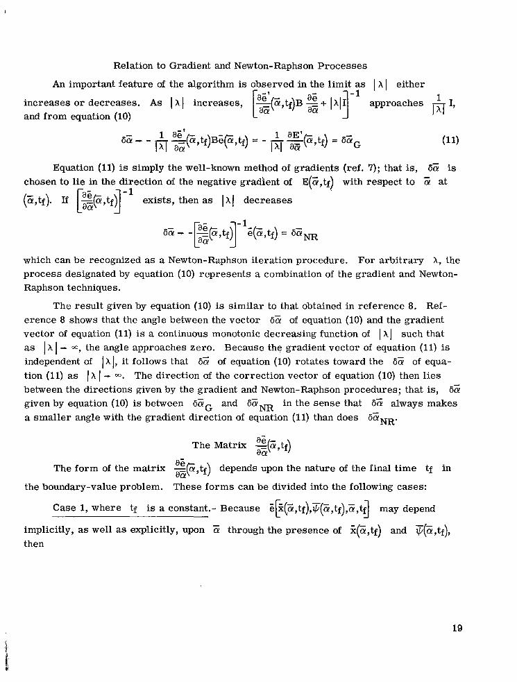
Relation to Gradient and Newton- Raphs on Processes

An important feature of the algorithm is observed in the limit as I XI either

increases o r decreases. As I XI increases, [%z,tf)B 5 + 1 X I g - l approaches and from equation (10)

a 5

Equation (11) is simply the well-known method of gradients (ref. 7); that is, 6a! is chosen to lie in the direction of the negative gradient of E(a!,tf> with respect to a! at

(5,tf). Jf [%F,tf]-' exists, then as 1x1 decreases

which can be recognized as a Newton-Raphson iteration procedure. For arbitrary X, the process designated by equation (10) represents a combination of the gradient and Newton- Raphson techniques.

The result given by equation (10) is similar to that obtained in reference 8. Ref- erence 8 shows that the angle between the vector 6 5 of equation (10) and the gradient vector of equation (11) is a continuous monotonic decreasing function of I X I such that as I X I - 00, the angle approaches zero. Because the gradient vector of equation (11) is independent of 1x1, it follows that 6a! of equation (10) rotates toward the 6 5 of equa- tion (11) as l X I - 03. The direction of the correction vector of equation (10) then l ies between the directions given by the gradient and Newton-Raphson procedures; that is, 6z given by equation (10) is between 6aG and 6Zm in the sense that 6 5 always makes a smaller angle with the gradient direction of equation (11) than does 6ZNR.

a5 - The Matrix ,,(a,tf)

The form of the matrix %F,tf) depends upon the nature of the final time tf in a a the boundary-value problem. These forms can be divided into the following cases:

Case 1, where tf is a constant.- Because ~[%(~, t f ) ,~(Z, t f ) ,Z , t f l may depend - .

implicitly, as well as explicitly, upon 5 through the presence of Z(5,tf) and T(Z,tf), then

19

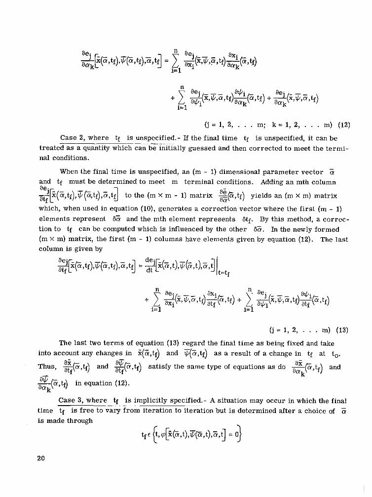
(j = 1, 2, . . . m; k = 1, 2, . . . m) (12)

treated as a qu.antity which can be initially guessed and then corrected to meet the termi- nal conditions.

Case 2, where tf is unspecified.- If the final t ime tf is unspecified, it can be

When the final time is unspecified, an (m - 1) dimensional parameter vector a! and tf must be determined to meet m terminal conditions. Adding an mth column

yF(Z, t f ) , s (Gtf ) ,a ! , td to the (m X m - 1) matrix %p,tf) yields an (m X m) matrix

which, when used in equation (lo), generates a correction vector where the first (m - 1) elements represent 6z and the mth element represents 6tf. By this method, a correc- tion to tf can be computed which is influenced by the other 6E. In the newly formed (m x m) matrix, the first (m - 1) columns have elements given by equation (12). The last column is given by

atf aa

(j = 1, 2, . . . m) (13)

The last two te rms of equation (13) regard the final t ime as being fixed and take into account any changes in %(Z,tf) and $(a!,tf) as a result of a change in tf at to.

/

Thus, -(Z,tf) a 5 and -(a,$) aiJ - satisfy the same type of equations as do --F,tf) ax and - atf atf q w f ) in equation (12). '@k

Case 3, where tf is implicitly specified.- A situation may occur in which the final

t ime tf is free to vary from iteration to iteration but is determined after a choice of a!

20

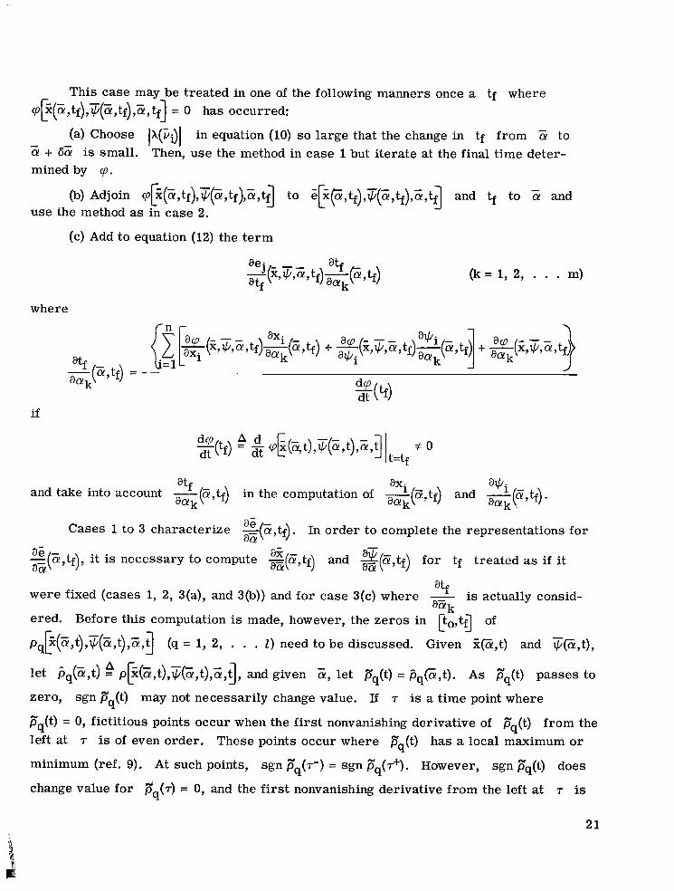
This case may be treated in one of the following manners once a tf where

(a) Choose lX(Fi)l

cp~(~,tf),s(a!,tf),a!,tf] = 0 has occurred:

in equation (10) so large that the change in tf from a to a + 6a! is small. Then, use the method in case 1 but iterate at the final time deter- mined by cp.

- -

(b) Adjoin cp[%(~,tf),~(a!,tf),a!,t~ to sbF,tf),q(a!,Q),a!,tg and tf to a! and

(c) Add to equation (12) the term

use the method as in case 2.

where

(k = 1, 2, . . . m)

if

%(tf) = cpx(@t),q a!,t),a!,t # 0 A d c ( 11 t=tf

and take into account -(Z,tf) in the computation of -(Z,tf) axi and r(a,t f) . a*i - @ k .

aG - Cases 1 to 3 characterize G(a,tf). In order to complete the representations for -

=(a,tf), as - it is necessary to compute =(Z,tf) a: and g(E, t f ) for tf treated as if it a@

aEk were fixed (cases 1, 2, 3(a), and 3(b)) and for case 3(c) where - is actually consid-

ered. Before this computation is made, however, the zeros in po,tf3 of

pq[%(Z,t),q(Z,t),Z,j (q = 1, 2, . . . 1 ) need to be discussed. Given %@,t) and q@,t),

let fiq(Z,t) = A p[%(a!,t),&!,t),Cy,d, and given a!, let pq(t) = p,(Z,t). As pq(t) passes to

zero, sgn p” (t) may not necessarily change value. If T is a time point where

Eq(t) = 0, fictitious points occur when the first nonvanishing derivative of pq(t) from the left at T is of even order. These points occur where p” (t) has a local maximum or

minimum (ref. 9). At such points, sgn p” (7-) = sgn Fq(.r+). However, sgn Fq(t) does

change value for 5 (7) = 0, and the first nonvanishing derivative from the left at T is q

q

q

q

21

of odd order. These values of T, denoted by t*, are referred to as switching points of the switching function Fq(t) to distinguish them from zeros'of &(t) where sgn Fq(t) does not change sign. Let the set of switching points of Eq(t) be denoted by Sq(t*) and S(t*) denote the set of all switching points of all fJq(t) (q = 1, 2, . . . I ) . Because the total number of switching points is assumed to be finite, the elements of S(t*) can be ordered such that

S(t*) = (t;, ti, . . . t;) where tT+l > tt for i = 1, 2, . . . v.

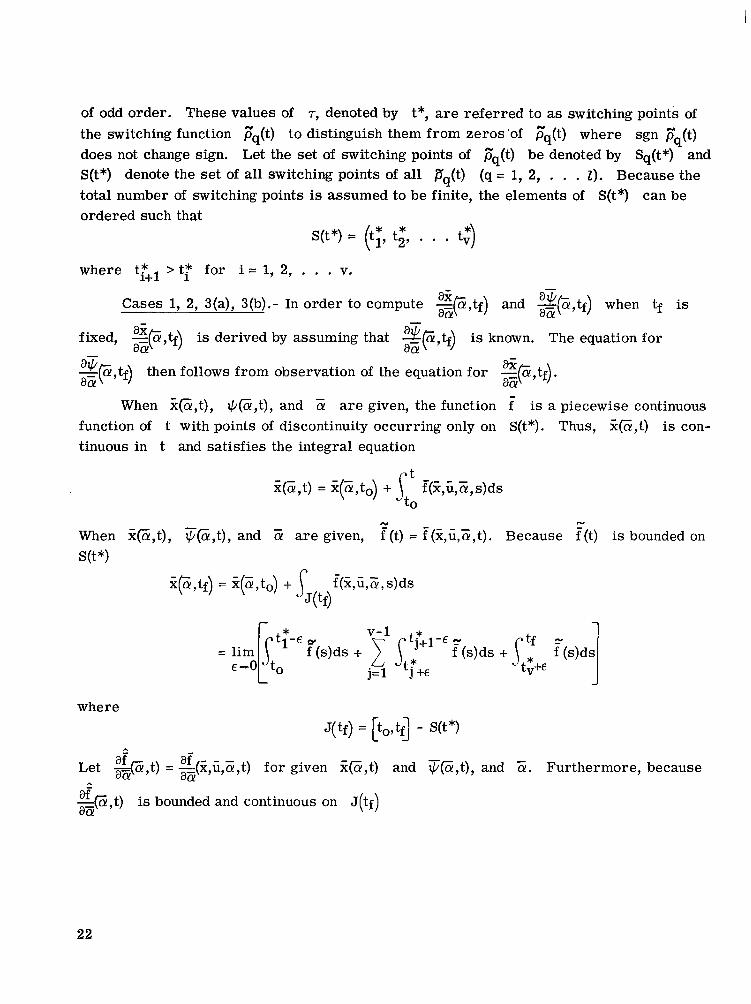
Cases 1, 2, 3(a), 3(b).- In order to compute s(Z,tf) and %(E,tf) when tf is a 0 a 0 - fixed, %(E,Q) is derived by assuming that %p,Q) is known. The equation for

zp,tf) then follows from observation of the equation for z@,tf). a 0 aa

a 0 When :@,t), J/@,t), and a! a r e given, the function f is a piecewise continuous

function of t with points of discontinuity occurring only on S(t*). Thus, %@,t) is con- tinuous in t and satisfies the integral equation

t

to %@,t) = %(z,to) + 1 f(f,u,z,s)ds

Y - - - _ N When f@,t), Ffi,t), and a! are given, f (t) = f (x,u,@,t). Because f(t) is bounded on S(t*)

* = l i m k t 1 - E f (s)ds + 5' &:'-

j = 1 j + E €40 to

where

A

Let @,t) a i = =(%,G,a!,t) aT for given Z@,t) and F(Z,t), and E . Furthermore, because

a 0

A a 0 - s @ , t ) is bounded and continuous on J(tf)

22

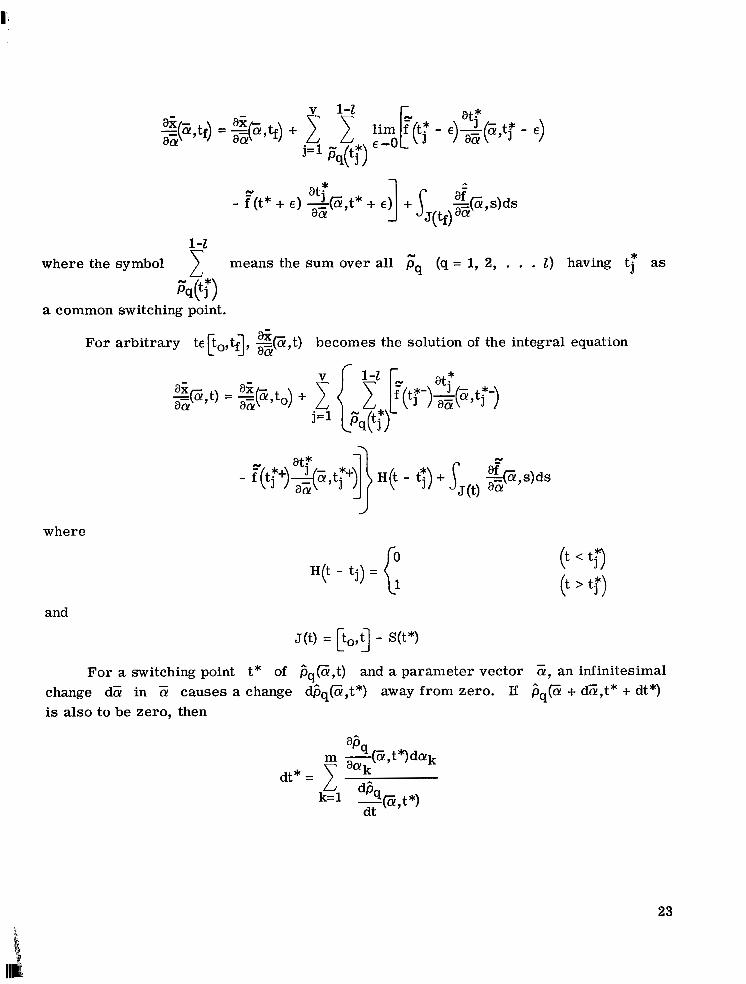
N at* - f (t* + E ) A@,t* + E ) + %@,s)ds a a 1 s.(w'

1 means the sum over all Fq (q = 1, 2, . . . 2) having t j * as

qti) where the symbol

a common switching point.

For arbitrary t e becomes the solution of the integral equation

where

and

(t < ti) (t > t?)

J(t) = po,CJ - S(t*) -

For a switching point t* of d,@,t) and a parameter vector CY, an infinitesimal change da! in a! causes a change dbq@,t*) away from zero. If bq@ + dZ,t* + dt*) is also to be zero, then

23

where

n

i= 1

and

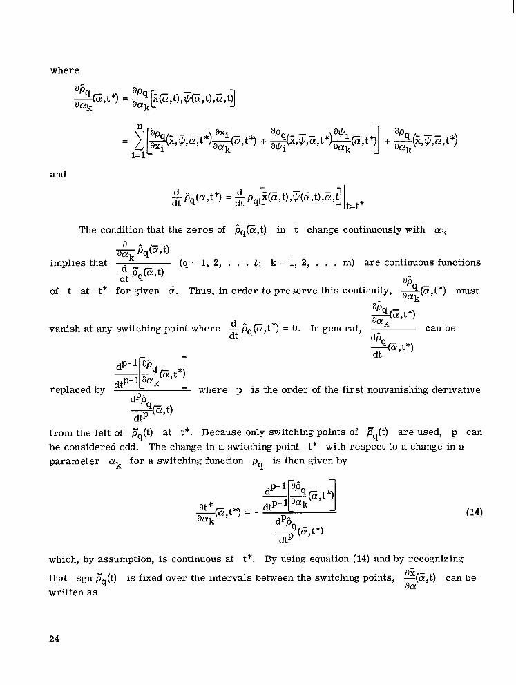
The condition that the zeros of cq@,t) in t change continuously with a k a

i j q m implies that (q = 1, 2, . . . I ; k = 1, 2, . . . m) are continuous functions

of t at t* for given a. Thus, in order to preserve this continuity, A @ , t * ) must

g Fq@ ,t) - a6

--@,t*)

-@,t*)

G q

dt Gq can be d - vanish at any switching point where - pq@,t? = 0. In general,

dt e,[%@$*] dtP- 1

replaced by where p is the order of the first nonvanishing derivative dpb $@,S

from the left of pq(t) be considered odd. parameter a k for a switching function p is then given by

at t*. Because only switching points of 3 (t) are used, p can q The change in a switching point t* with respect to a change in a

q

at* -@,t*) = - dPbq -(Z,t*) dtP

which, by assumption, is continuous at t*. By using equation (14) and by recognizing ai? - that sgn Fq(t) is fixed over the intervals between the switching points, =(a,t) can be aa written as

24

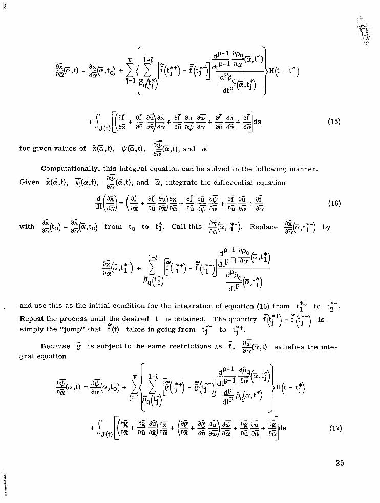
for givenvalues of %@,t), F@,t), %(Z,t), and Z. a a

Computationally, this integral equation can be solved in the following manner. - Given %@,t), T@,t), %@,t), and 5, integrate the differential equation a a

with - t a2 - a , t o ax from to to tT. Call this ,(a,t1 a: - *- ). Replace %(a,tl as- *- ) by a-,(o) = aJ- 1 a@

*- and use this as the initial condition for the integration of equation (16) from t? to t2 . Repeat the process until the desired t is obtained. The quantity f'($+) - ?(t(tf-) is simply the "jump" that r(t) takes in going from tr- to t?.

- Because is subject to the same restrictions as f , %,t) satisfies the inte- az

gra l equation

Computationally, equation (17) can be treated the same as equation (15). Given i5 and the solution of equation (2), equations (15) and (17) yield a simultaneous set of matrix

9 a!,tf for use in cases I, 2, integral equations for the determination of =@,tf) and a-(- ) 3(a), and 3(b). It can be noted that z(Z,t) and -!!(Z,t) a r e piecewise continuous func-

tions over Ct.,tf3 with discontinuities occurring on S(t*).

a% - aa! -

aa! aa

a! a

a+bi b i a@k The initial conditions -@,to) and -(a!,to) (i = 1, 2, . . . n;

k = 1, 2, . . . m) are to be determined from the nature of a! in a particular problem; for example, if a!1 = +b to 4 1

(i = 1)

(i = 2, . . . n) axi a@ and -(to) = 0 (i = 1, 2, . . . n; j = 1, 2, . . . n).

- a2 - a 0 aa

Case 3(c).- Let -(a,tf) and %(a!,tf), given by equations (15) and (17), be denoted

by X(5,tf) and 9(E,tf), respectively. In case 3(c), an extra term must be added to equations (15) and (17) so that they become

ZP,tf) = X(z,tf) + [%(a!,tf) + f (tf) -44 1::- and

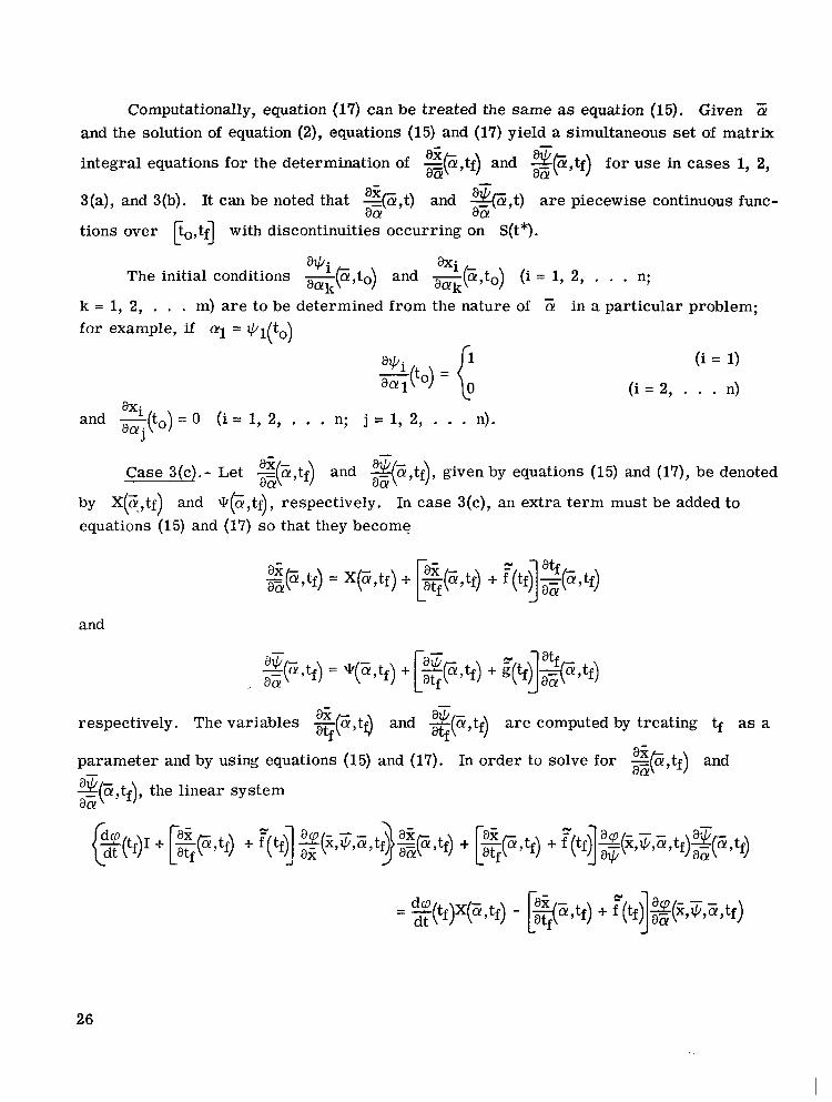
a2 respectively. The variables q p , t d and s ( Z , Q ) a r e computed by treating tf as a

parameter and by using equations (15) and (17). In order to solve for %(??,tf) and

%(E,+), the linear system

atf

- aa!

aa

= %Q(tf)X(Z7tf) dt - [$$Z,tf) + ?(tf$g)(z,?,Z,tf)

26

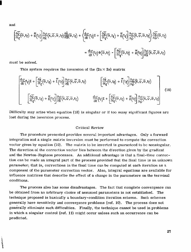
and

must be solved.

This system requires the inversion of the (2n X 2n) matrix

Difficulty may ar i se when equation (18) is singular o r if too many significant figures a r e lost during the inversion process.

Critical Review

The procedure presented provides several important advantages. Only a forward integration and a single matrix inversion must be performed to compute the correction vector given by equation (10). The matrix to be inverted is guaranteed to be nonsingular. The direction of the correction vector l ies between the direction given by the gradient and the Newton-Raphson processes. An additional advantage is that a final-time correc- tion can be made an integral part of the process provided that the final time is an unknown parameter; that is, corrections in the final time can be computed at each iteration as a component of the parameter correction vector. Also, integral equations a r e available for influence matrices that describe the effect of a change in the parameters on the terminal conditions.

The process also has some disadvantages. The fact that complete convergence can be obtained from an arbitrary choice of assumed parameters is not established. technique proposed is basically a boundary-condition iteration scheme. Such schemes generally have sensitivity and convergence problems (ref. 10). The process does not generally eliminate such difficulties. Finally, the technique cannot be used in problems in which a singular control (ref. 11) might occur unless such an occurrence can be predicted.

The

27

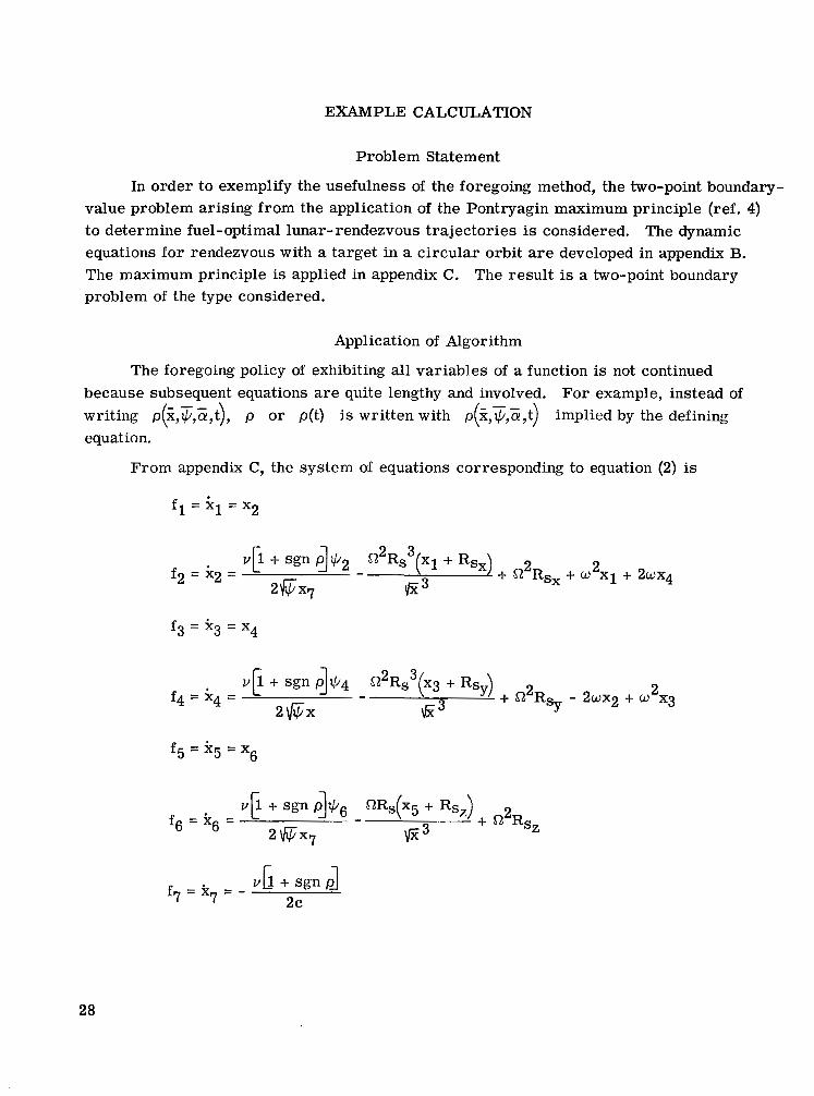
EXAMPLE CALCULATION

Problem Statement

In order to exemplify the usefulness of the foregoing method, the two-point boundary- value problem arising from the application of the Pontryagin maximum principle (ref. 4) to determine fuel-optimal lunar- rendezvous trajectories is considered. The dynamic equations for rendezvous with a target in a circular orbit are developed in appendix B. The maximum principle is applied in appendix C. The result is a two-point boundary problem of the type considered.

Application of Algorithm

The foregoing policy of exhibiting all variables of a function is not continued because subsequent equations are quite lengthy and involved. writing p(x,+,a,t), p or p(t) is written with p(%,+,a,t) implied by the defining equation.

For example, instead of -- - --

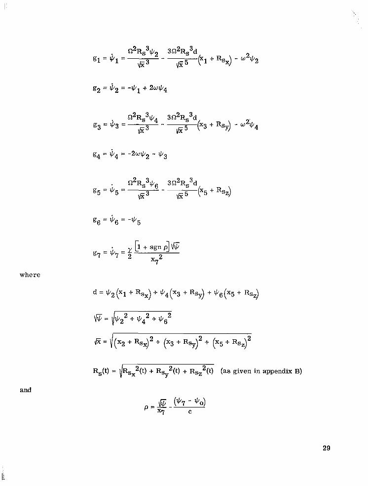
From appendix C, the system of equations corresponding to equation (2) is

f l = ir , = x2

f3 = kJ = x4

f5 = x5 = X6

28

$3 g4 = q4 = -20$2 -

where

Rs(t) = pSx2(t) + Rs 2(t) + RsZ 2 (t) (as given in appendix B) Y

and

29

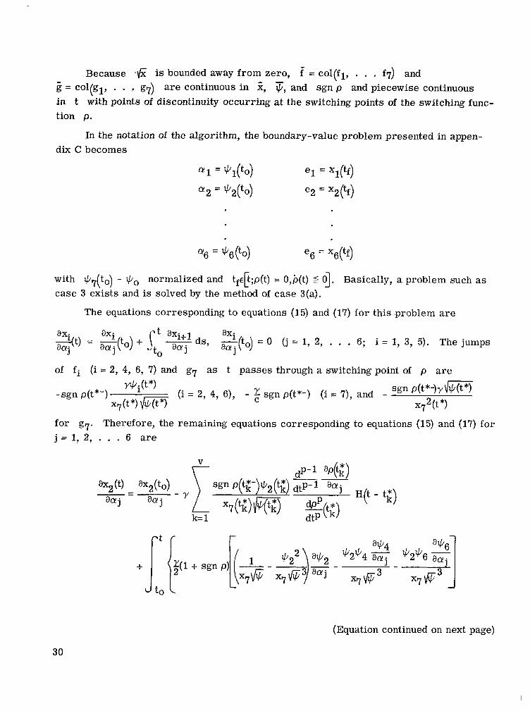
Because -6 is bounded away from zero, E = col(gl, . . .. 87) a r e continuous in x, Q, and sgn p and piecewise continuous in t with points of discontinuity occurring at the switching points of the switching func- tion p.

= col(f1, . . . f7) and - -

In the notation of the algorithm, the boundary-value problem presented in appen- dix C becomes

a1 = +l(tO)

a2 = q t o )

e1 = Xl(tf)

e2 = X2(tf)

with +7(to) - Q0 normalized and tfek;P(t) = O,b(t) 5 4. Basically, a problem such as case 3 exists and is solved by the method of case 3(a).

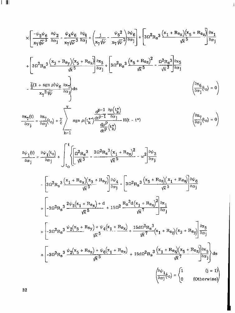
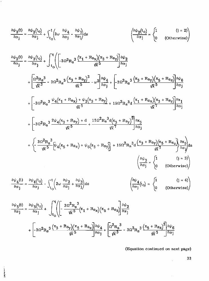
The equations corresponding to equations (15) and (17) for this problem a r e

axi axi -(t) = -t axi ( .) + it - ds, q(to) = 0 (j = 1, 2, . . . 6; i = 1, 3, 5). The jumps aolj aa j aa! j

0

of fi (i = 2, 4, 6, 7) and g7 as t passes through a switching point of p a r e

sgn P (t * -1 y m (i = 2, 4, 6), - 2! sgn p(t*-) (i = 7), and - rlC/,(t*)

x7(t*) vm- C x 7 W -sgn p(t*-)

for g7. Therefore, the remaining equations corresponding to equations (15) and (17) for j = 1, 2, . . . 6 are

(Equation continued on next page)

30

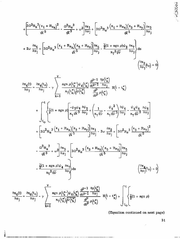
(Equation continued on next page)

31

(. + Rsy)(X5 + RSz] : Rs (X5 + Rsz)' --I- Q2RS3 8x5 + [ 2 3 3 352 Rs J ; r5 J aaj fi5 6 3 aaj

r I

32

2 3 & - wj% + [3522Rs3 (x3 + Rs~)(X5 +

E 5 a a j f i5 + - - [,,,, 3S-J Rs

fi3

2q4(x3 + Rsy + d

E5 1552

+

.cb(zw ( j = 4)

(Otherwise)

(Equation continued on next page)

33

( - = { (j = 6)

(Otherwise)

34

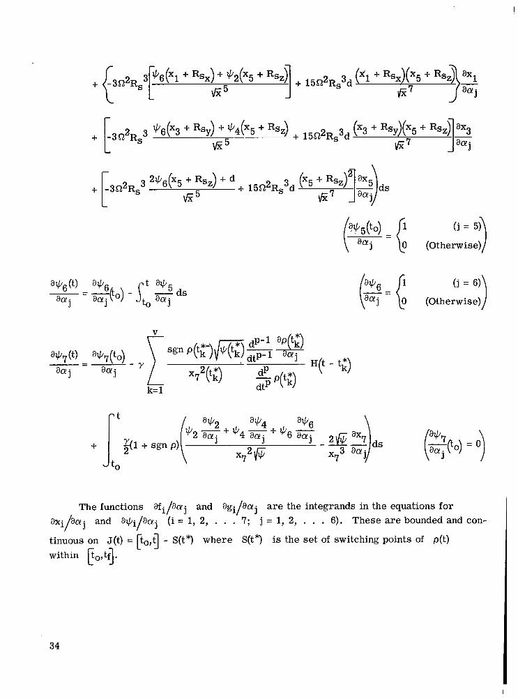
The functions afi/8aj and ag i /b j are the integrands in the equations for axi/acyj and aQi/aaj (i = 1, 2, . . . 7; j = 1, 2, . . . 6). These are bounded and con-

tinuous on J(t) = [to,g - S( t7 where S(t7 is the set of switching points of p(t) within p0,tf3.

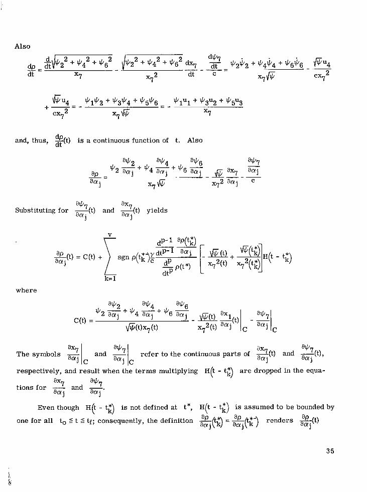
Also

and, thus, x(t) dP is a continuous function of t. Also

a'7 ax7 a n a 0 Substituting for -(t) and -(t) yields

where

ax a'7 refer to the continuous par ts of <(t) and -@I, The symbols - ax7 I c and zlc aaj

respectively, and result when the te rms multiplying H t - tc) are dropped in the equa-

and -. tions for - (

a'7 ax7 aa j aa j

Even though H(t - tz) is not defined at t*, H(t - tz) is assumed to be bounded by ap * ap *- renders -(t) aP

aci J one for all to s t s tf; consequently, the definition %(tk) = q ( t k )

35

continuous at tz. Time derivatives of ?%!@ are not continuous at tz because a a j 2 H(t - t*) is not bounded. In order to apply the algorithm, only the cases where the dt switching points of p(t) are simple zeros can be considered. For all such cases con- sidered, the number of zeros of p(t) were finite.

Finally, because a! = (al, * ' * "6)' and G(a!,tf) = (el, . . . e6)', the matrix

ZP,tf) is the (6 X 6) a r ray (axi/aaj) (i = 1, 2, . . . 6; j = 1, 2, . . . 6). The mea-

sure of terminal e r r o r is E(a!,tf) = 2 - 2 .

a a bixi (tf)

i= 1

Results

The algorithm and system equations were programed for the IBM 7094 electronic data processing system by using the Fortran IV language. Copies of the program are available on request from the Trajectory Applications Section, Langley Research Center, for the problem "Fuel Optimal Rendezvous" (program no. E1257). Integration was per- formed with fixed-step s izes of either 2 o r 4 seconds by using a method with a fourth- order Adams-Bashforth predictor formula and a fourth-order Adams-Moulton corrector formula.

The program was such that fixed-final-time and free-final-time solutions could be obtained. The program had the option of iteration at a fixed time or at a time when, after a specified number of coast periods have taken place, p = 0 and b 5 0. The approach taken in constructing free-time solutions was to begin with a nominal and to compute suc- cessively fixed-time solutions for increasing values of the final time until, at such a time, a zero of p(t) was observed, which satisfied a prescribed number of coasts with b 5 0. This solution was then used as a nominal with p(t) = 0 and b 5 0 as a stopping condition.

The satellite orbital plane was placed in the xy-plane of the rotating system. fig. B- 1 of appendix B.) Examples were computed both with the vehicle launched from absolute res t from the surface of the moon in the satellite plane and from absolute res t from out of plane. Table I shows the values of the fixed parameters for classes of both examples.

(See

36

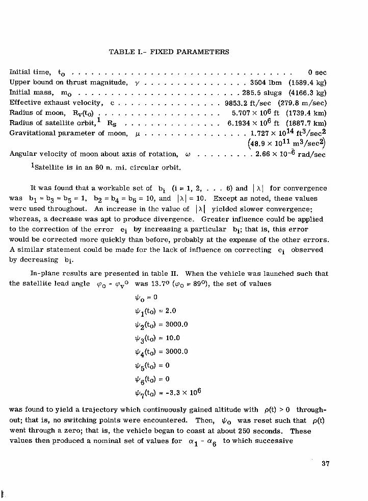
TABLE 1.- FIXED PARAMETERS

Initial time, to . . . . . . . . . . . . . . . . . . . . . . . Upper bound on thrust magnitude, y . . . . . . . . . . . . Initial mass, mo . . . . . . . . . . . . . . . . . . . . . . Effective exhaust velocity, c . . . . . . . . . . . . . . . . Radius of moon, Rv(to) . . . . . . . . . . . . . . . . . . Radius of satellite orbit, Rs . . . . . . . . . . . . . . . Gravitational parameter of moon, ,u . . . . . . . . . . . .

Angular velocity of moon about axis of rotation, w . . . .

. . . . . . . . . . . Osec

. . . . 3504 lbm (1589.4 kg)

. . . 285.5 slugs (4166.3 kg) 9853.2 ft/sec (279.8 m/sec)

5.707 X 106 f t (1739.4 km) 6.1934 X lo6 f t (1887.7 km)

. . . . 1.727 X 1014 ft3/sec2 (48.9 x 10l1 m3/sec2)

. . . . . 2.66 X 10-6 rad/sec

lSatellite is in an 80 n. mi. circular orbit.

It was found that a workable set of bi (i = 1, 2, . , . 6) and I XI for convergence was b l = b3 = b5 = 1, b2 = b4 = b6 = 10, and Ihl = 10. were used throughout. An increase in the value of I XI yielded slower convergence; whereas, a decrease was apt to produce divergence. Greater influence could be applied to the correction of the e r ro r would be corrected more quickly than before, probably at the expense of the other e r rors . A similar statement could be made for the lack of influence on correcting ei observed by decreasing bi.

Except as noted, these values

e i by increasing a particular bi; that is, this e r r o r

In-plane results a r e presented in table 11. When the vehicle was launched such that the satellite lead angle ‘po - ‘pvO was 13.70 (q0 = 89O), the set of values

= 0

*&to) = 2.0

+/,(to) = 3000.0

Q3(to) = 10.0

+/,(to) = 3000.0

+5(t0) = 0

=

+7(to) = -3.3 x 106

was found to yield a trajectory which continuously gained altitude with p(t) > 0 through- out; that is, no switching points were encountered. Then, was reset such that p(t) went through a zero; that is, the vehicle began to coast at about 250 seconds. These values then produced a nominal set of values for a1 - a6 to which successive

37

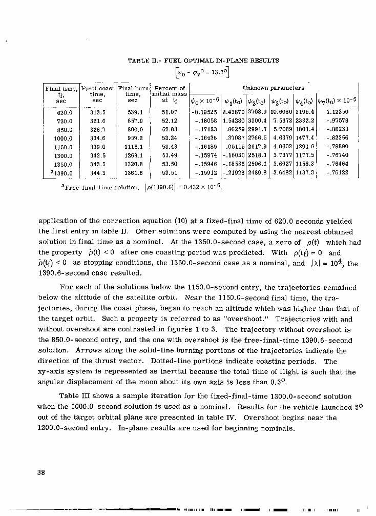
TABLE 11.- FUEL OPTIMAL IN-PLANE RESULTS

2.43870 1.54280

.86229

.37087

.05115 -.16030 -.18535 -.21928 - .

pinal time, tf ,

sec

3708.9 3300.4 2991.7 2766.5 2617.9 2518.1 2506.1 2489.8

620.0 720.0 850.0

1000.0 1150.0 1300.0 1350.0

'1390.6

._

First coast time, sec

313.5 321.6 328.7 334.6 339.0 342.5 343.5 344.3

.-

Final burn time, sec

539.1 657.9 800.0 959.2

1115.1 1269.1 1320.8 1361.6

-.

Percent of .nitial mass

a t tf

51.07 52.12 52.83 53.24 53.43 53.49 53.50 53.51

.

.-

$ox 10-6

-0.19525 -. 18058 -.17123 - .16 536 -.16189 -. 15974 -. 15946 -.15912

__ -

J

Unknown parameters

c/3 (to) .0.6080 7.5372 5.7089 4.6379 4.0602 3.7377 3.6927 3.6482

IC/, (to) 3195.4 2332.2 1801.4 1477.4 1291.6 1177.5 1156.3 1137.3

q t o ) x 10-5 . -

1.12350 -.97578 -.88233 -.82356 - .78890 - .76740 - .76464 -.76122

. .

aFree-final-time solution, )p(1390.6)1 = 0.432 x

application of the correction equation (10) at a fixed-final time of 620.0 seconds yielded the f i rs t entry in table 11. Other solutions were computed by using the nearest obtained solution in final time as a nominal. At the 1350.0-second case, a zero of p(t) which had the property b(t) < 0 after one coasting period was predicted. With p(tf) = 0 and p(tf) < 0 as stopping conditions, the 1350.0-second case as a nominal, and 1x1 = lo4, the 1390.6-second case resulted.

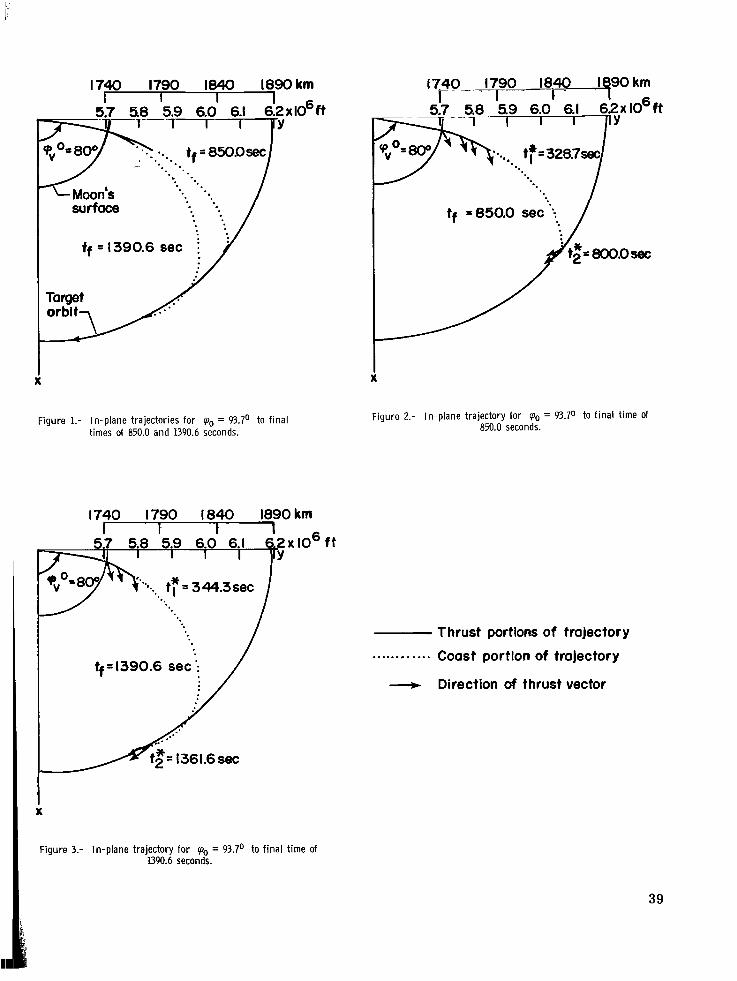
For each of the solutions below the 1150.0-second entry, the trajectories remained below the altitude of the satellite orbit. jectories, during the coast phase, began to reach an altitude which was higher than that of the target orbit. Such a property is referred to as "overshoot." Trajectories with and without overshoot are contrasted in figures 1 to 3. The trajectory without overshoot is the 850.0-second entry, and the one with overshoot is the free-final-time 1390.6-second solution. Arrows along the solid-line burning portions of the trajectories indicate the direction of the thrust vector. Dotted-line portions indicate coasting periods. The xy-axis system is represented as inertial because the total time of flight is such that the angular displacement of the moon about i t s own axis is less than 0.3'.

Near the 1150.0-second final time, the tra-

Table 111 shows a sample iteration for the fixed-final-time 1300.0-second solution when the 1000.0-second solution is used as a nominal. Results for the vehicle launched 5O out of the target orbital plane are presented in table IV. Overshoot begins near the 1200.0-second entry. In-plane results are used for beginning nominals.

38

1740 1790 1840 1890 - 5.9 6.0 6.1 6:2x

Y

. . -. . . . . . - . . . e. . . - . . . * . surface

ff = 1390.6 sec

Target

X t./ Figure 1.- In-plane trajectories for 'po = 93.7O to f inal

times of 850.0 and 1390.6 seconds.

km

IO6 ft

Figure 3.- In-plane trajectory for 'po = 93.7O to f inal t ime of 1390.6 seconds.

X

1740- 1790 . 1840 1$90 km

Figure 2.- In-plane trajectory for 'po = 93.70 to f inal time of 850.0 seconds.

f t

Thrust portions of trajectory

. . . . . . . . . . . . Coast portion of trajectory

_I) Direction of thrust vector

39

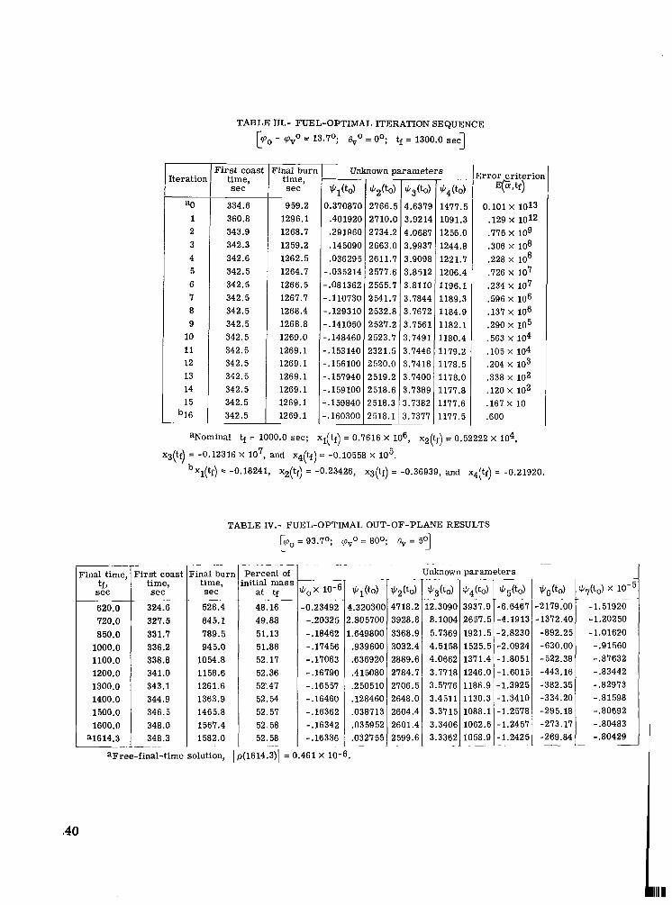
TABLE ID.- FUEL-OPTIMAL ITERATION SEQUENCE

@,(to)

2179.00 1372.40 -892.25 -630.00 -522.38 -443.16 -382.35 -334.20 -295.18 -273.17 -269.84 -

Final time, tf,

s ec

620.0 720.0 850.0

1000.0 1100.0 1200.0 1300.0 1400.0 1500.0 1600.0

a1614.3

-

lo-' -

-1.51920 - 1.20250 -1.01620

-.91560 -.87632 -.83442 -.82973 -.81598 -.80692 -.80483 -.80429 .- -

[teratior

a0 1 2 3 4 5 6 7 8 9

10 11 12 13 14 15

b16

_.

$/,(to)

L.320300 .805700 .649800 .939600 .636920 .415080 .250510 .128460 .038713 .035952 .032755

- -

tf = 1300.0 sec 1 rcpo - c p v ~ = 13.7O; $0 = o ;

*2(to)

4718.2 3928.8 3368.9 3032.4 2889.6 2784.7 2706.5 2648.0 2604.4 2601.4 2599.6

L

F i r s t coast time, s ec

334.6 360.8 343.9 342.3 342.6 342.5 342.5 342.5 342.5 342.5 342.5 342.5 342.5 342.5 342.5 342.5 342.5

$3(to)

2.3 09 0.~ 8.1004 5.7369 4.5158 4.0662 3.7718 3.5776 3.4511 3.3715 3.3406 3.3362

..

3na l burr time, s ec

$4(to)

393 7.9 2657.5 1921.5 1525.5 1371.4 1246.0 1186.9 1130.3 1088.1 1062.6 1058.9 -

959.2 1296.1 1268.7 1259.2 1262.5 1264.7 1266.5 1267.7 1268.4 1268.8 1269.0 1269.1 1269.1 1269.1 1269.1 1269.1 1269.1

49.88 51.13 51.88 52.17 52.36 5T.47 52.54 52.57 52.58 52.58 - .

~~

Unknown parameters

-.20325 -.18462 -.17456 -.17063 -.16790 -.16557 -.16460 -.16362 -.16342 -.16336

*/,(to)

0.370870 .401920 .291960 .145090 .036295

- .035214 - .08 1362 -.110730 -. 129310 -. 14 1050 -.148460 .. 153 140 .. 156100 ..157940 .. 159100 .. 159840 ..160300

___ *,(to) 2766.E 271o.c 2734.2 2663.0 2611.7 2577.6 2555.7 2541.7 2532.8 2527.2 2523.7 2321.5 2520.0 2519.2 2518.6 2518.3 2518.1 ~

$3 (to)

4.6375 3.9214 4.0687 3.9937 3.909E 3.8512 3.811G 3.7844 3.7672 3.7561 3.7491 3.7446 3.7418 3.7400 3.7389 3.7382 3.7377

~- *4 (to)

1477.5 1091.3 1256.0 1244.8 1221.7 1206.4 1196.1 1189.3 1184.9 1182.1 1180.4 1179.2 1178.5 1178.0 1177.8 1177.6 1177.5

Srror criterioi E(Ktf)

0.101 x 1013 .129 x 1012 .776 X lo9 .306 x lo8 .228 x lo8 .126 x 107 .234 x 107

.290 x 105 ,563 x 104 . io5 x 104 .204 x 103

.120 x 102

.596 x 106

.137 x lo6

.338 x lo2

.167 X 10

.600

aNominal tf = 1000.0 sec; xl(tf) = 0.7616 X lo6, xz(tf) = 0.52222 x lo4,

bxl(tf) = -0.18241, xz(tf) = -0.23426, x3(tf) = -0.36939, and x4(tf) = -0.21920.

xg(tf) = -0.12316 x lo7, and x&) = -0.10558 x lo5.

TABLE IV.- FUEL-OPTIMAL OUT-OF-PLANE RESULTS

Po = 93.70; 'pvo = 80°; = 501

. - -

time,

327.5 331.7 336.2

343.1

Percent of I nitial mass

. -

aFree-final-time solution, I p(1614.3)l = 0.461 X 10-

Unknown parameters -I - .. .- .

J/ 5 00)

- 6.6467 -4.1913 -2.8230 -2.0924 -1.8051 -1.6015 -1.3925 -1.3410 -1.2578 - 1.2457 - 1.2425 . .~ .

Running time for all cases on the IBM 7094 electronic data processing system was approximately 7 minutes. In programing this example, the primary objective w a s to decide whether the method could be applied to such a nonlinear two-point boundary-value problem and not necessarily to write a program giving solutions in a minimum of com- puter time. Time-consuming subroutines were included to test for conditions leading to numerical instability (overflow, underflow, and so forth) and to determine the nature of the zeros of the switching function. tions involved account for the rather long computer time. No sensitivity o r convergence problems were found in any of the cases considered.

These subroutines and the large number of equa-

CONCLUDING REMARKS

A successive approximation procedure for attacking a class of two-point boundary-

Basically, the boundary-value problem was one in which the optimal-control law value problems which frequently occurs in indirect optimization theory has been pre- sented. w a s piecewise continuous and in which there were a number of system parameters to be determined to meet an equal number of terminal conditions. An iterative logic was developed in which an assumed set of parameters would be improved upon so that, by repetitive use of a correction formula, a monotonic decreasing sequence af values of a positive definite function that measures the terminal e r r o r s was produced.

The procedure provided several important advantages. A forward integration and a The matrix single matrix inversion must be performed to compute the correction vector.

to be inverted w a s guaranteed to be nonsingular. was found to lie between the direction given by the gradient and the Newton-Raphson pro- cedures. An additional advantage w a s that a final-time correction could be made an integral part of the process provided that the final time was an unknown parameter; that is, corrections in the final time would be computed at each iteration as a component of the parameter correction vector. that describe the effect of a change in the parameters on the terminal conditions.

The direction of the correction vector

Integral equations were derived for influence matrices

The process also had some disadvantages. The fact that complete convergence could be obtained from an arbitrary choice of assumed parameters was not established. The technique proposed is basically a boundary-condition iteration scheme. generally have sensitivity and convergence problems. eliminate such difficulties, but none were found in the example considered. technique cannot be used in problems in which a singular control might occur unless such an occurrence can be predicted.

Such schemes The process does not generally

Finally, the

In order to demonstrate the usefulness of the procedure, solutions were obtained to the two-point boundary-value problem resulting from an application of the Pontryagin

4 1

maximum principle to obtain fuel-optimal lunar- rendezvous trajectories for a target in a circular orbit. Fixed- and free-final-time solutions were computed for planar and nonplanar situations. Running t imes on the IBM 7094 electronic data processing system were on the order of ‘7 minutes. In programing this example, the primary objective was to decide whether the method could be applied to such a nonlinear two-point boundary- value problem and not necessarily to write a program giving solutions in a minimum of computer time. Time-consuming subroutines were included to test for conditions leading to numerical instability (overflow, underflow, and so forth) and to determine the nature of the zeros of the switching function. These subroutines and the large number of equations involved accounted for the rather long computer time.

Langley Research Center, National Aeronautics and Space Administration,

Langley Station, Hampton, Va., May 8, 1968, 125-19-04-01-23.

42

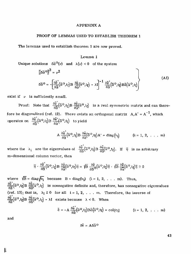
APPENDIX A

PROOF OF LEMMAS USED TO ESTABLISH THEOREM 1

The lemmas used to establish theorem 1 are now proved.

Lemma 1

Unique solutions 6Eo(v) and X(v) < 0 of the system

ll6E01l2 = v2 1

exist if v is sufficiently small.

Proof: Note that --=.(Eo,tf)B ae' -(E aG ,tf) is a real symmetric matrix and can there- a@ a 0 fore be diagonalized (ref. 12). There exists an orthogonal matrix A,A' = A - l , which operates on ---(a ae' -0 , tf ) B - ae ai(a -O,tf ) to yield

- 1 ae -o ae -o

A :(a a a ,tf)B =(a a@ ,tf)A' = diag(Xi) (i = 1, 2, . . . m)

ae ' -o tf 3 -o az where the X i a r e the eigenvalues of -(a , )

m-dimensional column vector, then

aE(a ,tf). If 17 is an arbitrary

where = diagfi because B = diag(bi) (i = 1, 2, . . . m). Thus, -(a -0,tf ) B - a6 (E ,tf) is nonnegative definite and, therefore, has nonnegative eigenvalues a@ a 5

ae l a@ a 0

(ref. 13); that is, X i 2 0 for all i = 1, 2, . . . m.

-(Eo,tf)B %@o,tf) - X I exists because X < 0. When

Therefore, the inverse of

and

ae ' -o a 0 C = -A -(a ,tf)BZPO,tf) = COl(Ci) (i = 1, 2, . . . m)

6? = A6Eo

43

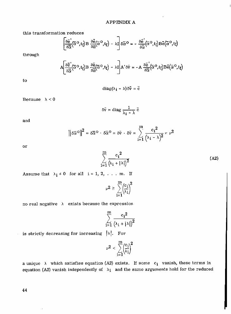
APPENDIX A

this transformation reduces

F F o , t $ B ,tf) - X I SZ0 = - =(a ae' -o , t f ) B ~ ( ~ o , t f ) aa 1

through

to

Because X < O

diag(Xi - X)6V = C

6; = diag - l c X i - X

and

o r m

i= 1

Assume that X i # 0 for all i = 1, 2, . . . m. If

no real negative X exists because the expression

L 2 i=l ( X i + 1x1)

is strictly decreasing for increasing 1x1. For

a unique X which satisfies equation (A2) exists. If some ci vanish, these te rms in equation (A2) vanish independently of X i and the same arguments hold for the reduced

44

APPENDIX A

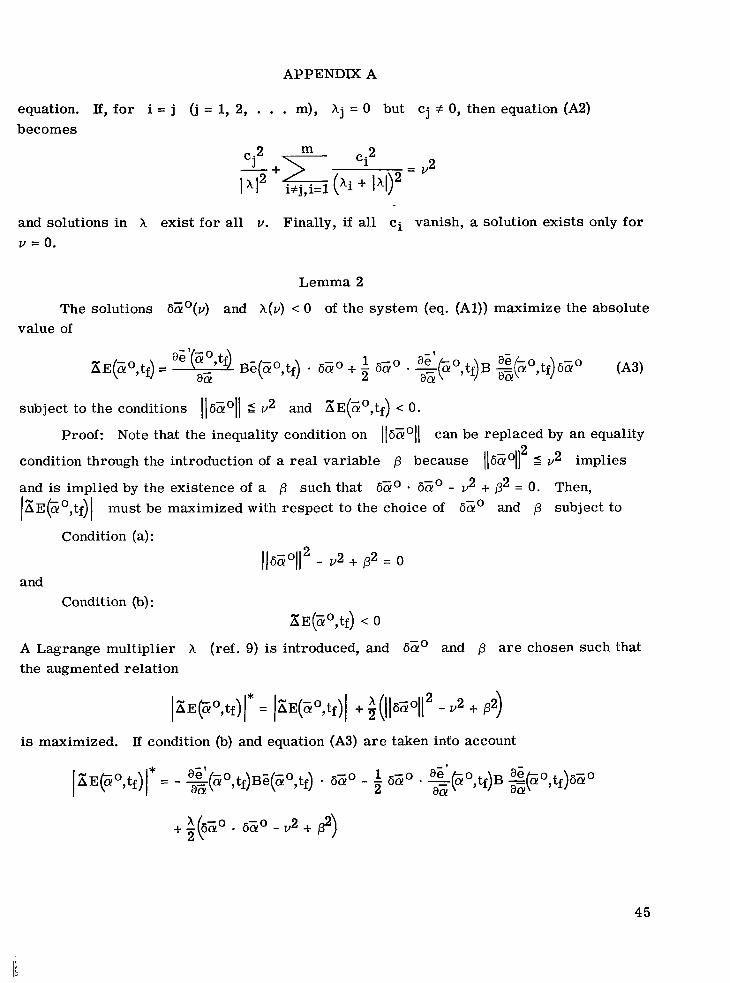
equation. If, fo r i = j (j = 1, 2, . . . m), X j = 0 but C j f 0, then equation (A2) becomes

and solutions in X exist for all v. Finally, if all c i vanish, a solution exists only for v = 0.

Lemma 2

The solutions 6zo(v) and X(v) < 0 of the system (eq. (Al)) maximize the absolute value of

subject to the conditions 116cYoll S v2 and aE(Z0,tf) < 0.

Proof: Note that the inequality condition on l16Zoll can be replaced by an equality 2

condition through the introduction of a real variable p because 116zol] 2 v2 implies

and is implied by the existence of a p such that 6E0 * 6E0 - v2 + p2 = 0. Then, lxE(Eo,tf)I must be maximized with respect to the choice of 6Eo and p subject to

Condition (a) :

))6zoJ12 - v2 + p2 = 0 and

Condition (b): xE(Eo,tf) < 0

A Lagrange multiplier X (ref. 9) is introduced, and 6zo and p a r e chosen such that the augmented relation

is maximized. If condition (b) and equation (A3) a r e taken info account

45

II I l l l l l l l l l I1 IIIII ll1111111Il1111111

APPENDIX A *

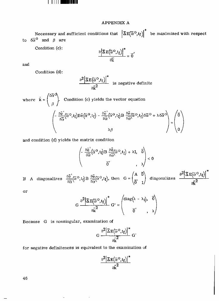
Necessary and sufficient conditions that 1 xE(Zo,tf)l be maximized with respect to 65' and p a r e

Condition (c) :

and

Condition (d):

a2 I EE (5 O, tf ) [ * is negative definite

aii2

where k = (6zT. Condition (c) yields the vector equation

and condition (d) yields the matrix condition

\ - t

0 *

A D a21 xE(5 O, tf) I If A diagonalizes --&!",tf)B ae' aT;p O,tf), then G = (6, diagonalizes

aE2 or

Because G is nonsingular, examination of

aG" for negative definiteness is equivalent to the examination of

ai;"

46

APPENDIX A

- 1

Thus, "E(Zo7tf) is negative definite in 6Zo because I A 1 # 0 and %po,tf)B =-=(a a5 -o ,tf) a@

is nonnegative definite. Therefore, k(zo,tf) = 0 if and only if 675' = 0.

h

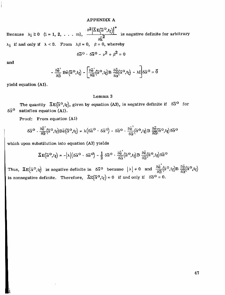
Because X i 2 0 (i = 1, 2, . . . m), is negative definite for arbitrary aii2

Xi if and only if X < 0. From X p = 0, p = 0, whereby

650 * 6ZO - ,2 + p2 = 0

and

yield equation (Al) . Lemma 3

The quantity KE(Eo7tf), given by equation (A3), is negative definite if 65' for

Proof: From equation (Al)

6z0 satisfies equation (Al).

which upon substitution into equation (A3) yields

47

APPENDIX B

DYNAMIC EQUATIONS FOR LUNAR-RENDEZVOUS PROBLEM

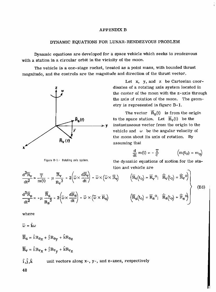
Dynamic equations are developed for a space vehicle which seeks to rendezvous with a station in a circular orbit in the vicinity of the moon.

The vehicle is a one-stage rocket, treated as a point mass, with bounded thrust magnitude, and the controls are the magnitude and direction of the thrust vector.

Z Q)

J X

Figure B-1.- Rotating axis system.

Let x, y, and z be Cartesian coor- dinates of a rotating axis system located in the center of the moon with the z-axis through the axis of rotation of the moon. The geom- etry is represented in figure B-I.

The vector Rs(t) is from the origin to the space station. Let &(t) be the instantaneous vector from the origin to the vehicle and w be the angular velocity of the moon about its axis of rotation. assuming that

By

a T - m(t) = - - at C

the dynamic equations of motion for the sta- tion and vehicle are -

1 - - -=- - d2% T &7 - 2 (- w x - :) - - w x ( W X R , - > (&(to) = %o; Rv(to) = iivo) dt2 m(t) ’

- -- d2Es RS 2 w X - (- d?) - O X - (- u X R S - )

- - I J . 3 - dt2 RS

where

- A

Rv = iRvx + ~ R v + GRvz Y

9J - (Es(to) = E s O ; Rs(to) = Rs

i,i,ii 48

unit vectors along x-, y-, and z-axes, respectively

APPENDIX B

m (t) total vehicle mass

I-L universal gravitational constant multiplied by mass of moon

- T thrust control vector of vehicle

T magnitude of ?

C effective exhaust velocity of vehicle rockets

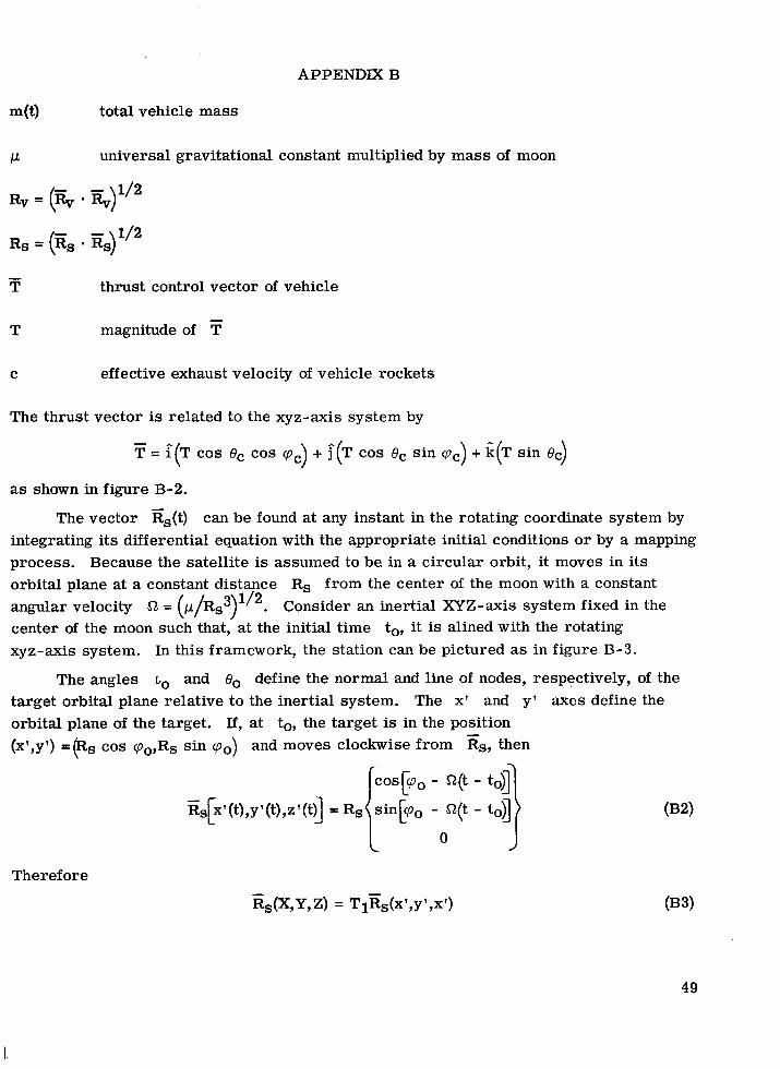
The thrust vector is related to the xyz-axis system by - T = :(T cos ec cos qc) + i ( ~ cos ec sin qc) + C(T sin ec)

as shown in figure B-2.

The vector Es(t) can be found at any instant in the rotating coordinate system by integrating its differential equation with the appropriate initial conditions o r by a mapping process. Because the satellite is assumed to be in a circular orbit, it moves in its orbital plane at a constant distance Rs from the center of the moon with a constant angular velocity S2 = (p/RS3)'l2. Consider an inertial XYZ-axis system fixed in the center of the moon such that, at the initial time to, it is alined with the rotating xyz-axis system. In this framework, the station can be pictured as in figure B-3.

The angles L~ and 8, define the normal and line of nodes, respectively, of the target orbital plane relative to the inertial system. The x' and y' axes define the orbital plane of the target. If, at to, the target is in the position (x',y') =Ps cos qO,Rs sin qo) and moves clockwise from Rs, then

-

Theref ore

49

I.

APPENDIX B

I k

Q I

Figure 8-2.- Reference axis system fo r control vector.

X

F igu re B-3.- Station viewed in ine r t i a l axis system.

where -

8, -cos L~ sin eo sin L~ sin 8,

Bo cos L~ cos eo -sin c0 cos eo 1 -

sin L~ cos Lo L o -

Because the q z - a x i s system rotates about the Z-axis with a constant angular velocity w

cos w(t - to)

-sin w(t - to)

sin w( t - to)

cos w(t - to)

0 0

50

APPENDM B

or

Also

with

and

- to)

- to>

cos w(t - to)

-sin o(t - to)

0

o r

(Equation continued on next page)

51

APPENDIX B

- to) - eo (W COS Lo + 0) 3 7 0

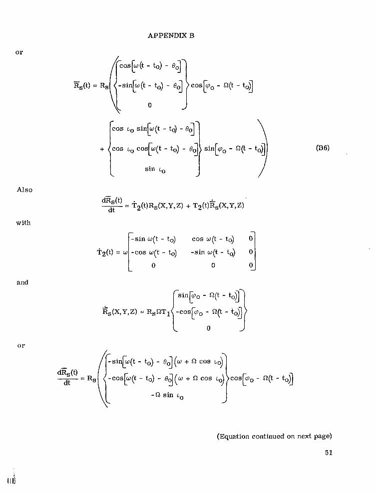
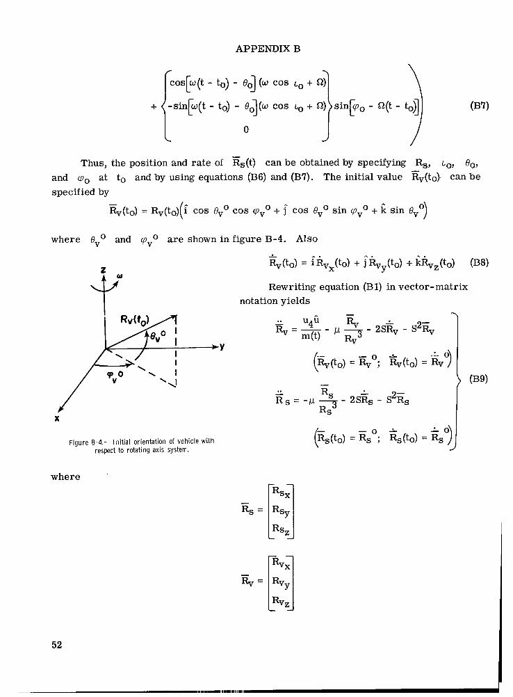
Thus, the position and rate of &(t) can be obtained by specifying Rs, L ~ , eo, and ‘po at to and by using equations (B6) and (B7). The initial value &(to)- can be specified by

- Rv(to) = Rv(to)(i cos Qvo cos qVo + 3 cos OVo s in ‘pvo + sin Ova)

where Bvo and ‘pvo a r e shown in figure B-4. Also

J X

Rewriting equation (Bl) in vector-matrix notation yields

1 (%(to) = - 0 Rv ; - Rv(to) = GvO)

Figure 8-4.- Initial orientation of vehicle with respect to rotating axis system.

where

52

APPENDIX B

and

cos Bc cos cpc 3 = [ o s ec sin q]

sin OC u3 -

- -w 0

s = l 0 0 0

0 - - -

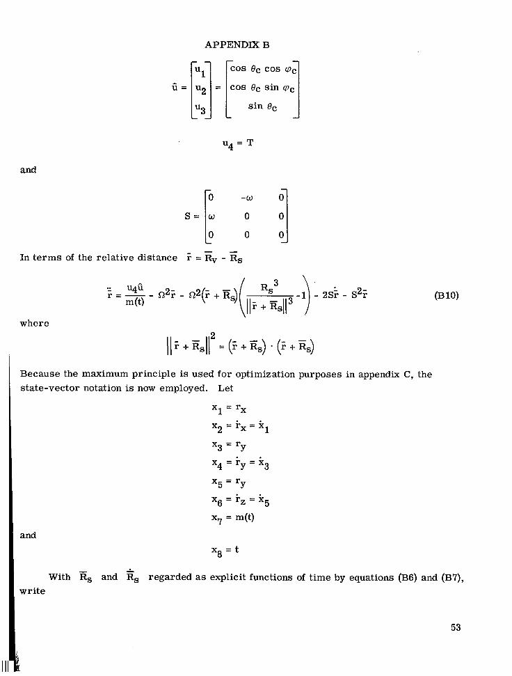
In te rms of the relative distance E = Rv - Rs

\

where

Because the maximum principle is used fo r optimization purposes in appendix C, the state-vector notation is now employed. Let

x1 = rx

x2 = rx =

x3 = ry

x4 = ry = x3

x5 = ry

x6 = rz = x

x7 = m(t)

%

5

and X8 = t

With Rs and & regarded as explicit functions of time by equations (B6) and (B7), write

53

APPENDIX B

u4 x 7 = - c

t0

t f

M =

N =

K =

54

0 1 0 0 0 0

- 0 1 0 0 0 0 - - 0 0 0 0 0 0

launch time

final rendezvous time

- 0 0 0 0 0 0 1 0 0 0 0 1 -

0 0 0 0 0 0 0 1 0 0 0 0

0 0 0 0 0 0 -1 0 0 0 0 0

0 0 0 0 0 0

0 1 0 0 0 0

0 0 0 0 0 1

0 0 0 0 0 0

.. .. . - .

APPENDIX B

0 0 0 0 0 0 0 0 0 0 0

L = I : : : : ] 0 0 0 0 0 0

0 0 0 0 0 0

0 0 0 0 A = [ 0 1 0 0

0 0 0 1 0

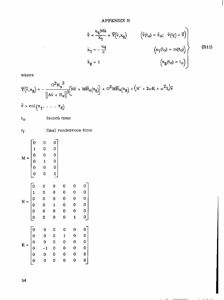
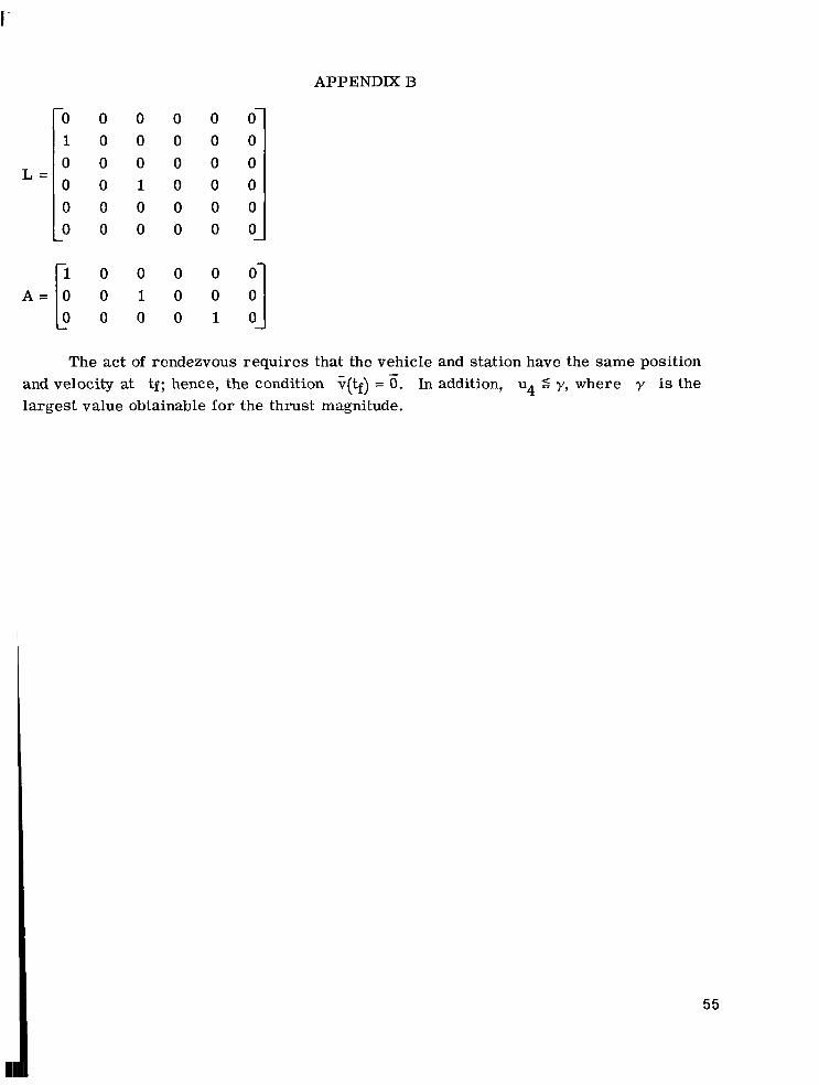
The act of rendezvous requires that the vehicle and station have the same position and velocity at tf; hence, the condition c(tf) = 0. In addition, u4 5 y, where y is the largest value obtainable for the thrust magnitude.

55

APPENDIX C

NECESSARY CONDITIONS FOR FUEL-OPTIMAL RENDEZVOUS

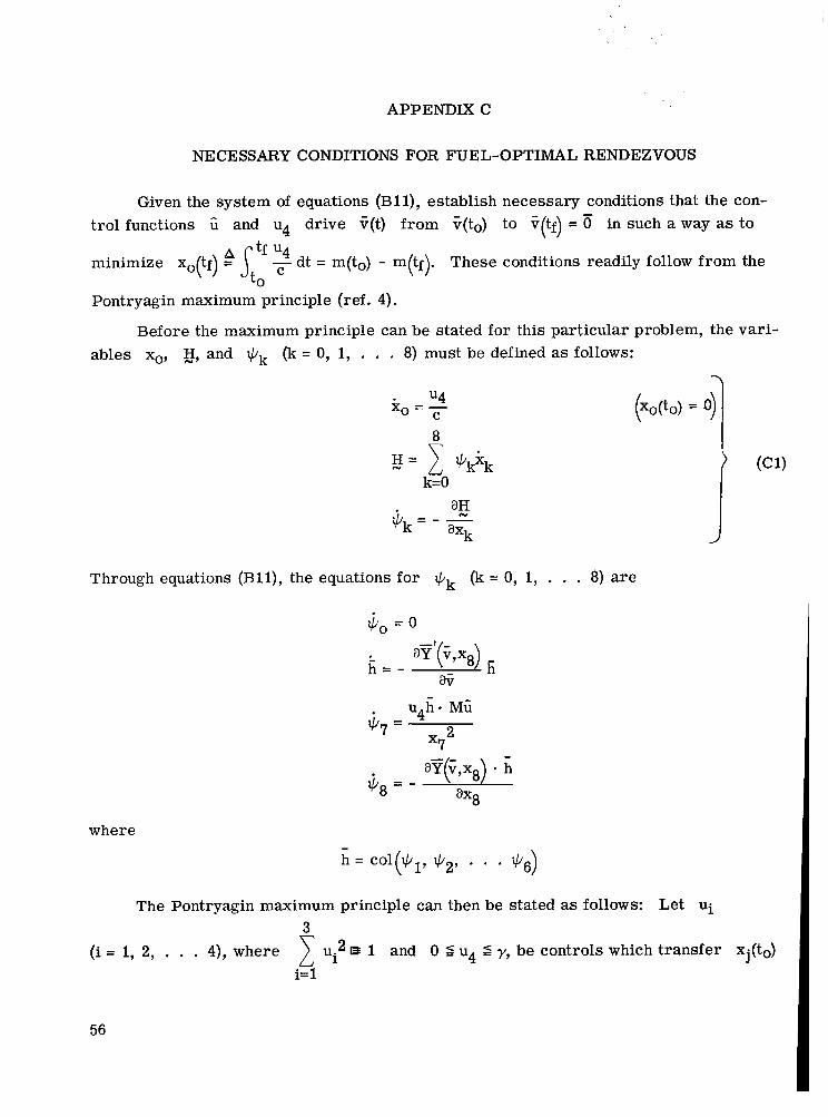
Given the system of equations (Bll), establish necessary conditions that the con- trol functions 6 and u4 drive ?(t) from G(to) to ?(tf) = 0 in such a way as to

minimize x .( t f) s,t’ 2 dt = m(to) - m(tf). These conditions readily follow from the

Pontryagin maximum principle (ref. 4).

-

0

Before the maximum principle can be stated for this particular problem, the vari- ables xo, 5, and +k (k = 0, 1, . . . 8) must be defined as follows:

* u4 xo = - C

J aH + k = - - axk

N

Through equations (Bll), the equations for +k (k = 0, 1, . . . 8) a r e

$Lo = 0

The Pontryagin maximum principle can then be stated as follows: Let ui 3

(i = 1, 2, . . . 4), where 1 u: 1 and 0 5 u4 S y, be controls which transfer xj(to) i= 1

56

APPENDIX C

to xj(tf) there exist a nonzero continuous vector with elements mined by equation (Cl) such that:

( j = 0, 1, . . . 8). In order that U i minimize xo(tf), it is necessary that

@j ( j = 0, 1, . . . 8) as deter-

(1) For every t (to 5 t 2 tf), the function E(xj,@j,ui), for fixed x j and @j,

attains i ts maximum Pdpj,@j) at the point ui = Ui(t); that is, g[@j,Xj,Ui(tg = v ( + j , X j ) .

If equations (Bll), (Cl), and €€[@j,xj,ui(tU = h4(Qj,Xj) a r e satisfied, then q0 5 0 and

gpj(t),+j(t)l = 0.

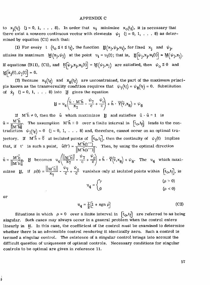
(2) Because x7(4) and x8(Q) a r e unconstrained, the part of the maximum princi- ple known as the transversality condition requires that q7(tf) = @8(tf) = 0. Substitution of xj ( j = 0, 1, . . . 8) into E gives the equation

If M'h f 0, then the 6 which maximizes E and satisfies fi - 6 = 1 is

u = - M'fi . The assumption M'fi = 0 over a finite interval in Fo,tf3 leads to the con- I 1 M 'dl

tradiction qj(tf) = 0 ( j = 0, 1, . . . 8) and, therefore, cannot occur on an optimal tra-

jectory. If M'fi = 0 at isolated points of ko,tf3, then the continuity of qj(t) implies

that, if t ' is such a point, 6(t') = *. M'G t" Then, by using the optimal direction M ' fi( t ' -)I

I

u = - 5 becomes u4 flM'fill - - 71-7 +7 ".) + ~ . Y v x - - (-, 8) + @8' The u4 which maxi- IlM'~lI' x7 *7 @o mizes u, if p(t) = - l l M " ' l - - C + vanishes only at isolated points within po,tf3, is

x7

or

= xk + sgn 4 u4 2

Situations in which p 0 over a finite interval in po,tf] a r e referred to as being singular. Such cases may always occur in a general problem when the control enters linearly in H. In this case, the coefficient of the control must be examined to determine whether there is an admissible control rendering it identically zero. Such a control is termed a singular control. The existence of a singular control brings into account the difficult question of uniqueness of optimal controls, Necessary conditions for singular controls to be optimal are given in reference 11.

-

57

APPENDIX C

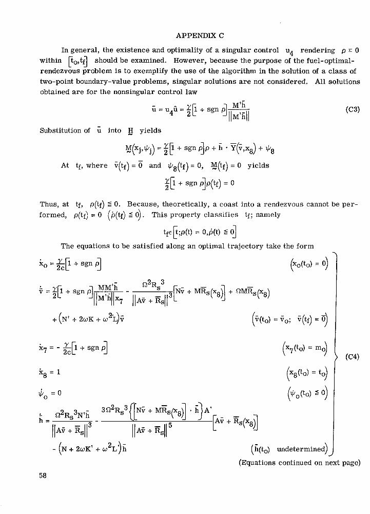
In general, the existence and optimality of a singular control u4 rendering p = 0 within po,tf3 should be examined. However, because the purpose of the fuel-optimal- rendezvous problem is to exemplify the use of the algorithm in the solution of a class of two-point boundary-value problems, singular solutions are not considered. All solutions obtained a r e for the nonsingular control law

Substitution of into E yields

At tf, where v(tf) = 0 and +,(tf) = 0, E(tf) = 0 yields

2 Z ~ + s g n p p t f c 1 0 = O

Thus, at tf, p(tf) 2 0. Because, theoretically, a coast into a rendezvous cannot be per- formed, p(tf) = 0 (b(tf) 2 0). This property classifies tf; namely

tfeE;p(t) = O,b(t) 6 OJ 1

The equations to be satisfied along an optimal trajectory take the form

+ (N' + 2wK + w2L)C (?(to) = to; V(tf) = Ti)

k8 = 1

+bo = 0

- (N + 2wK' + w2Ljh (;(to) undetermined) -I

(Equations continued on next page)

58

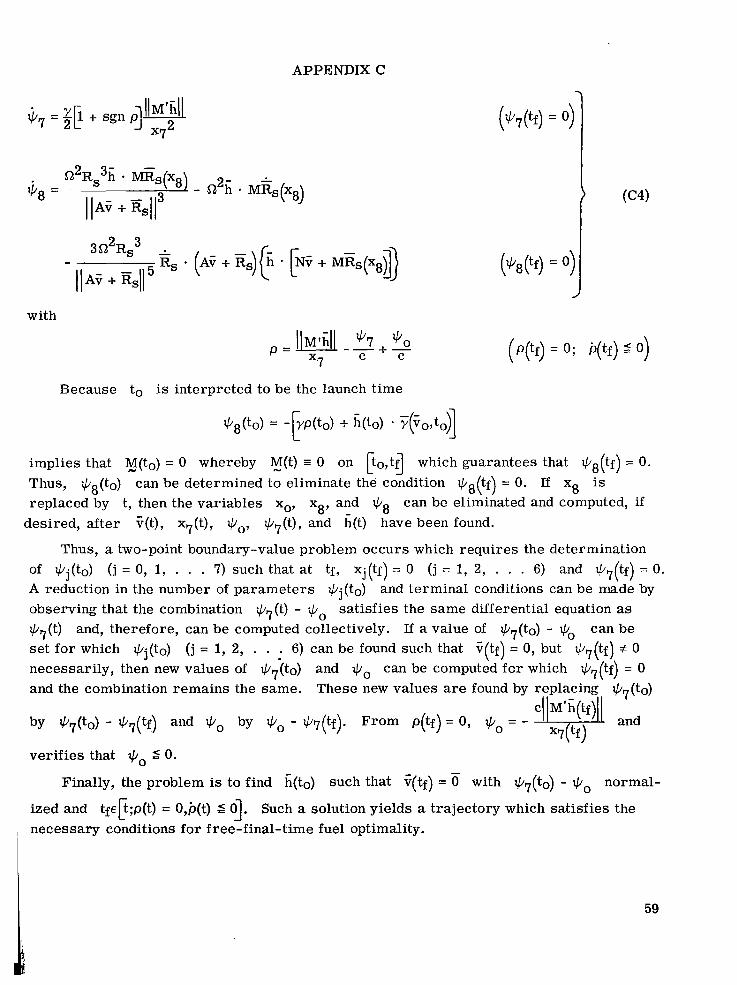
APPENDIX C

+L7 = 5 [ 1 + sgn p ]llM'Lll x72

with

Because to is interpreted to be the launch time

(P(tf) = 0; b(tf) 5 0)

implies that $(to) = 0 whereby y( t ) = 0 on po,tf3 which guarantees that +8(tf) = 0. Thus, q8(t0) can be determined to eliminate the condition @,(tf) = 0. If x8 is replaced by t, then the variables xo, x8, and +8 can be eliminated and computed, if

Thus, a two-point boundary-value problem occurs which requires the determination

desired, after ?(t), x7(t), q0, q7(t), and h(t) have been found.

of +j(to) A reduction in the number of parameters +j(to) observing that the combination q7(t) - Go satisfies the same differential equation as q7(t> and, therefore, can be computed collectively. If a value of +7(to) - Go can be se t for which +j(to) necessarily, then new values of +?(to)

( j = 0, 1, . . . 7) such that a t tf, Xj(tf) = 0 (j = 1, 2, . . . 6 ) and e7(tf) = 0. and terminal conditions can be made by

( j = 1, 2, . . . 6) can be found such that v tf = 0, but <b7(tf) f 0 -( 1 and q0 can be computed for which +,(tf) = 0

and the combination remains the same.

by +7(to) - +7(tf) and qo by +o - +7(tf)-

These new values are found by replacing +/,(to)

From P 0 tf = 0, + 0 =

verifies that 5 0.

Finally, the problem is to find K(t0) such that G(tf) = 0 with +7(to) - Qo normal-

ized and tfEF;p(t) = O,b(t) d q. Such a solution yields a trajectory which satisfies the , necessary conditions for free-final-time fuel optimality.

59

APPENDIX C

In conclusion, if tf is fixed, *8(tf) does not necessarily equal zero (ref. 4) in which case *8(tf) can be adjusted to satisfy lJ(tf> = 0 and, thus, eliminate the necessity of p(tf) = 0. If a solution can be obtained with p(tf) arbitrary but ZF/, 2 0, then the tra- jectory satisfies the necessary conditions of the Pontryagin maximum principle for fixed-final-time fuel optimality.

60

REFERENCES

1. Bryson, A. E.; and Denham, W. F.: A Steepest-Ascent Method for Solving Optimum Programming Problems. June 1962, pp. 247-257.

Trans. ASME, Ser. E: J. Appl. Mech., vol. 29, no. 2,

2. Kelley, Henry J.: Gradient Theory of Optimal Flight Paths. ARS, vol. 30, no. 10, Oct. 1960, pp. 947-954.

3. Mitter, S.; Lasdon, L. S.; and Waren, A. D.: The Method of Conjugate Gradients for Optimal Control Problems. Proc. IEEE, vol. 54, no. 6, June 1966, pp. 904-905.

4. Pontryagin, L. S.; Boltyanskii, V. G.; Gamkrelidze, R. V.; and Mishchenko, E. F.: The Mathematical Theory of Optimal Processes. Interscience Publ., c. 1962.

5. Gelfand, I. M.; and Fomin, S. V. (Richard A. Silverman, transl.): Calculus of Varia- tions. Prentice-Hall, Inc., c. 1963.

6. Bellman, Richard E.; and Dreyfus, Stuart E.: Applied Dynamic Programming. Princeton Univ. Press, 1962.

7. Saaty, Thomas L.; and Bram, Joseph: Nonlinear Mathematics. McGraw-Hill Book CO., c.1964, pp. 53-88.

8. Marquardt, Donald W.: An Algorithm for Least-Squares Estimation of Nonlinear Parameters. J. SOC. Ind. Appl. Math., vol. 11, no. 2, June 1963, pp. 431-441.

9. Hancock, Harris: Theory of Maxima and Minima. Dover Publ., Inc., 1960.

10. Merriam, C. W., 111: Optimization Theory and the Design of Feedback Control Sys- tems. McGraw-Hill Book Co., c.1964, pp. 235-284.

11. Kelley, Henry J.; Kopp, Richard E.; and Moyer, H. Gardner: Singular Extremals. Topics in Optimization, George Leitmann, ed., Academic Press, 1967, pp. 63- 101.

12. Margenau, Henry; and Murphy, George Moseley: The Mathematics of Physics and Chemistry.

13. Perlis, Sam: Theory of Matrices. Addison-Wesley Pub. Co., Inc., c.1952.

D. Van Nostrand Co., Inc., c.1943, p. 316.

NASA-Langley, 1968 - 19 L-5786 1 61

NATIONAL AERONAUTICS AND SPACE ADMINISTRATION WASHINGTON, D. C. 20546

OFFICIAL BUSINESS FIRST CLASS MAIL

POSTAGE A N D FEES PA11 NATIONAL AERONAUTICS i

SPACE ADMINISTRATION

“The aeronautical and space activities of the United States shall be condzicted so as t o contribute . . . to the expansion of human knowl- edge of pheno?iiena in the atmosphere and space. T h e Adniinistration shall provide for the widest practicable ai2d appropriate disseininatioit of information concerning its actitdies and the resalts thereof.”

-NATIONAL AERONAUTICS A N D SPACE ACT OF 1958

NASA SCIENTIFIC AND TECHNICAL PUBLICATIONS

TECHNICAL REPORTS: Scientific and technical information considered important, complete, and a lasting contribution to existing knowledge.

TECHNICAL NOTES: Information less broad in scope but nevertheless of importance as a contribution to existing knowledge.

TECHNICAL MEMORANDUMS : Information receiving limited distribution because of preliminary data, security classifica- tion, or other reasons.

CONTRACTOR REPORTS: Scientific and technical information generated under a NASA contract or grant and considered an important contribution to existing knowledge.

TECHNICAL TRANSLATIONS: Information published in a foreign language considered to merit NASA distribution in English.

SPECIAL PUBLICATIONS : Information derived from or of value to NASA activities. Publications include conference proceedings, monographs, data compilations, handbooks, sourcebooks, and special bibliographies.

TECHNOLOGY UTILIZATION PUBLICATIONS: Information on technology used by NASA that may be of particular interest in commercial and other non-aerospace applications, Publications include Tech Briefs, Technology Utilization Reports and Notes, and Technology Surveys.

Details on the availability of these publications may be obtained from:

SCIENTIFIC AND TECHNICAL INFORMATION DIVISION

NATIONAL AERO N AUT1 C S AND SPACE ADM I N ISTRATI ON Washington, D.C. 20546