A cloudification methodology for high performance simulations · Tesis Doctoral A Cloudification...
144
UniversityCarlosIIIofMadrid ComputerScienceandEngineeringDepartment ComputerArchitectureGroup Ph.D.PrograminComputerScienceandTechnology A Cloudification Methodology for High Performance Simulations Author: Alberto García Fernández Supervisors: Prof. Jesús CarreteroPérez Prof. Félix GarcíaCarballeira Lega a n é s, February 2016
Transcript of A cloudification methodology for high performance simulations · Tesis Doctoral A Cloudification...

University Carlos III of Madrid Computer Science and Engineering Department
Computer Architecture Group
Ph.D. Program in Computer Science and Technology
A Cloudification Methodology for High Performance Simulations
Author:
Alberto García Fernández
Supervisors:
Prof. Jesús Carretero Pérez
Prof. Félix García Carballeira
Legaanés, February 2016

Tesis Doctoral
A Cloudification Methodology for High Performance Simulations
AUTOR: Alberto Garcia Fernandez
DIRECTORES: Jesus Carretero Perez
Felix Garcia Carballeira
Firmas del Tribunal Calificador
(Nombre y apellidos) Firma
Presidente:
Secretario:
Vocal:
En Lega´nes, a de del 201

“I am prepared to go anywhere, provided it be forward.”
David Livingstone
Let us assure our readers that to the extent this article is imperfect, it is not a sin we have
committed knowingly.
Justin Kruger and David Dunning
Take a look what you’ve started
In the world flashing from your eyes
And you know that you’ve got it
From the thunder you feel inside
I believe in the feeling
All the pain that you left to die
Believe in believing
In the life that you give to try
I’ve lost my fear to what appears
I do my best
You seem surprised and realize
That’s in your eyes
The world is mine
The World is Mine by David Guetta

UNIVERSITY CARLOS III OF MADRID
Abstract
School of Engineering
Computer Science and Engineering Department
Ph.D. Program in Computer Science and Technology
A Cloudification Methodology for High Performance Simulations
by Alberto Garcia Fernandez
Many scientific areas make extensive use of computer simulations to study complex real-world
processes. These computations are typically very resource-intensive and present scalability issues
as experiments get larger, even in dedicated supercomputers since they are limited by their
own hardware resources. Cloud computing raises as an option to move forward into the ideal
unlimited scalability by providing virtually infinite resources, yet applications must be adapted
to this paradigm.
The major goal of this thesis is to analyze the suitability of performing simulations in clouds by
performing a paradigm shift, from classic parallel approaches to data-centric models, in those
applications where that is possible. The aim is to maintain the scalability achieved in traditional
HPC infrastructures, while taking advantage of Cloud Computing paradigm features. The thesis
also explores the characteristics that make simulators suitable or unsuitable to be deployed on
HPC or Cloud infrastructures, defining a generic architecture and extracting common elements
present among the majority of simulators.
As result, we propose a generalist cloudification methodology based on the MapReduce paradigm
to migrate high performance simulations into the cloud to provide greater scalability. We anal-
ysed its viability by applying it to a real engineering simulator and running the resulting imple-
mentation on HPC and cloud environments. Our evaluations will aim to show that the cloudified
application is highly scalable and there is still a large margin to improve the theoretical model
and its implementations, and also to extend it to a wider range of simulations.

UNIVERSIDAD CARLOS III DE MADRID
Resumen
Escuela Politecnica Superior
Departamento de Informatica
Doctorado en Ciencia y Tecnologıa Informatica
Una Metodologıa de ”Cloudificacion” para Simulaciones de Alto Rendimiento
por Alberto Garcia Fernandez
Muchas areas de investigacion hacen uso extensivo de simulaciones informaticas para estudiar
procesos complejos del mundo real. Estas simulaciones suelen hacer uso intensivo de recursos,
y presentan problemas de escalabilidad conforme los experimentos aumentan en tamano incluso
en clusteres, ya que estos estan limitados por sus propios recursos hardware. Cloud Computing
(computacion en la nube) surge como alternativa para avanzar hacia el ideal de escalabilidad
ilimitada mediante el aprovisionamiento de infinitos recursos (de forma virtual). No obstante,
las aplicaciones deben ser adaptadas a este nuevo paradigma.
La principal meta de esta tesis es analizar la idoneidad de realizar simulaciones en la nube
mediante un cambio de paradigma, de las clasicas aproximaciones paralelas a nuevos modelos
centrados en los datos, en aquellas aplicaciones donde esto sea posible. El objetivo es mantener
la escalabilidad alcanzada en las tradicionales infraestructuras HPC, mientras se explotan las
ventajas del paradigma de computacion en la nube. La tesis explora las caracterısticas que
hacen a los simuladores ser o no adecuados para ser desplegados en infraestructuras cluster o en
la nube, definiendo una arquitectura generica y extrayendo elementos comunes presentes en la
mayorıa de los simuladores.
Como resultado, proponemos una metodologıa generica de cloudificacion, basada en el paradigma
MapReduce, para migrar simulaciones de alto rendimiento a la nube con el fin de proveer mayor
escalabilidad. Analizamos su viabilidad aplicandola a un simulador real de ingenierıa, y eje-
cutando la implementacion resultante en entornos cluster y en la nube. Nuestras evaluaciones
pretenden mostrar que la aplicacion cloudificada es altamente escalable, y que existe un amplio
margen para mejorar el modelo teorico y sus implementaciones, y para extenderlo a un rango
mas amplio de simulaciones.


Acknowledgements
Cuando empec la tesis doctoral, imagine (supongo que como todo el mundo) que al acabarla
serıa la persona mas feliz del mundo, y que gritarıa y reirıa dando saltos de alegrıa. Ahora, tras
mas de cinco anos, resulta muy complicado describir el conjunto de sentimientos que tengo en
mi interior. No ha sido facil, no todo ha sido felicidad, y sinceramente, no se si valdra la pena.
Pero sı se que lo mejor de este viaje son las personas que me han acompanado por el camino.
Los ”agradecimientos” presentan poco espacio y resulta difıcil resumir mis sentimientos, ası que
no me queda mas remedio que ser parco en palabras. Pero si alguno se queda con ganas de mas,
puede preguntarme. Siempre me han dicho que soy muy frio. Sirva esto como promesa de que
intento (e intentare) que no sea ası.
A mi madre y a mi padre, Cristina y Eduardo, por ser el pilar silencioso que siempre esta ahı, y
porque soy lo que soy gracias a vosotros.
A mis hermanos Eduardo, Marcos, y a Gea. Porque en tiempos de dificultad, basta una charla
con ellos para sentirse mejor y volver a la batalla.
A Yago, porque tambien es mi puto hermano. Te quiero. Tus virtudes son inmensas, y tus
defectos hacen de la vida un lugar mas divertido.
A Carlos, porque este camino lo he andado junto a el, dıa a dıa, todos estos anos. Y si el no
hubiese estado ahı, puede que yo no hubiese llegado a la meta.
A Silvina, porque sin ella esta tesis no habrıa sido posible. Llego en el momento mas indicado.
Gracias a su esfuerzo descubrı el camino. Me diste (y me sigues dando) las fuerzas necesarias.
A la cuadrilla de practicas, Fran, Rafa, y Estefanıa. Porque gracias a sus risas y a su companerismo
prefiero ir al trabajo antes que no ir.
Al resto del grupo ARCOS, por haberme ayudado y ensenado todos estos anos. Porque he sacado
de vosotros todo el conocimiento que poseo.
A Gabriel, por ser mi companero de cervezas y batallas en los cortos dıas y en las largas noches
de Rumania. Porque t hablas mucho y yo muy poco, y por eso hacemos buena pareja.
A mis amigos de los grupos de los ”malloles”, los ”farmas”, y los ”g*****s de la uc3m”. Sois
demasiados y no os puedo poner, pero todos y cada uno habeis alegrado mi existencia dıa a dıa,
semana a semana, durante todos estos anos.
A Jesus y a Felix. Porque no me puedo imaginar jefes y directores mejores que ellos. Hay
doctorandos que acaban peleados con sus directores de tesis. Nunca he entendido por que.
vii


Contents
Abstract iv
Resumen v
Acknowledgements vii
List of Figures xiii
List of Tables xv
Abbreviations xvii
1 Introduction 1
1.1 Definition and Scope .............................................................................................................. 1
1.2 Motivation ............................................................................................................................... 2
1.3 Objectives ................................................................................................................................ 4
1.4 Structure and Contents ......................................................................................................... 5
2 State of the Art 7
2.1 High-Performance Computing ............................................................................................. 7
2.1.1 HPC Infrastructure Elements .................................................................................. 7
2.1.2 HPC Programming Models ...................................................................................... 8
2.1.3 Current Supercomputers and Petascale Systems .................................................. 9
2.1.4 Future Goals: Green HPC, Exascale Infrastructures, and Big Data .................. 10
2.2 Cloud Computing .................................................................................................................. 11
2.2.1 Infrastructure as a Service .......................................................................................12
2.2.2 Platform as a Service ................................................................................................13
2.2.3 Software as a Service ............................................................................................... 14
2.2.4 The Upcoming Anything as a Service Model ......................................................... 15
2.2.5 Current Challenges in Cloud Computing.............................................................. 16
2.2.6 Trends in Cloud Migration and Adaptation Techniques ....................................... 18
2.3 MapReduce ............................................................................................................................ 19
2.3.1 Hadoop MapReduce .................................................................................................21
2.3.2 HDFS ......................................................................................................................... 22
2.3.3 First Generation MapReduce Runtime (MRv1)................................................... 23
2.3.4 Next Generation MapReduce (MRv2) and YARN ................................................... 24
2.4 Cloud Computing and Scientific Applications .................................................................. 25
2.5 Summary................................................................................................................................ 26
3 Problem Statement 27
3.1 Problem Types ...................................................................................................................... 28
ix

Contents x
3.1.1 Pleasingly Parallel Problems .................................................................................. 28
3.1.2 Loosely Coupled Problems .....................................................................................30
3.1.3 Tightly Coupled Problems ......................................................................................30
3.1.4 Multivariate analysis: A Pleasingly Problem Particular Case ............................ 31
3.1.5 Problem Types, Infrastructures and Platforms ................................................... 32
3.2 Problem Statement: Applying Parallelism to Current Simulators ................................. 33
3.2.1 Generic Architecture of a Modern Simulator ....................................................... 34
3.2.2 Parallelization Layers .............................................................................................. 36
3.2.3 Computational Complexity ..................................................................................... 37
3.3 Case Study: RPCS ................................................................................................................ 40
3.3.1 Application Description ......................................................................................... 40
3.3.2 Algorithm .................................................................................................................. 41
3.3.3 RPCS Problem Stack ............................................................................................... 42
3.3.4 RPCS Analysis .......................................................................................................... 44
3.4 Summary ................................................................................................................................ 46
4 High Performance Computing Approaches to Problem Decomposition 49
4.1 Domain Decomposition Approaches in HPC .................................................................... 50
4.1.1 Domain Decomposition Using a Coordinator Process ....................................... 50
4.1.2 Domain Decomposition Using Collective I/O ...................................................... 52
4.1.3 Communication and Resource Modelling ............................................................ 53
4.2 Matrix Decomposition Approaches in HPC ...................................................................... 57
4.2.1 Matrix Decomposition Using Master-Slaves ....................................................... 58
4.2.2 Communication and Resource Modelling Example: LU Inversion................... 58
4.3 Application to RPCS ............................................................................................................ 62
4.3.1 Domain Decomposition in RPCS ........................................................................... 63
4.3.2 Matrix Decomposition in RPCS ............................................................................. 64
4.4 Evaluation .............................................................................................................................. 66
4.4.1 Domain Decomposition Evaluation ...................................................................... 67
4.4.2 Matrix Decomposition Evaluation ........................................................................ 69
4.5 Summary ................................................................................................................................ 69
5 A Methodology to Migrate Simulations to Cloud Computing 73
5.1 Methodology Description .................................................................................................... 73
5.1.1 Methodology Terms and Definitions ..................................................................... 74
5.1.2 Application Analysis ................................................................................................ 75
5.1.3 Cloudification Process Design ............................................................................... 76
5.1.4 Virtual Cluster Planning ......................................................................................... 79
5.2 Application to RPCS ............................................................................................................ 81
5.2.1 RPCS Application Analysis ..................................................................................... 81
5.2.2 RPCS Cloudification Process Design ..................................................................... 82
5.2.3 Implementation and platform configuration ...................................................... 82
5.3 Evaluation ..............................................................................................................................84
5.3.1 Execution Environments and Scenarios ..............................................................84
5.3.2 Results Discussion ................................................................................................... 85
5.4 Summary ............................................................................................................................... 88
6 Multivariate Analysis of Simulation Problems 91
6.1 Multivariate Analysis on Current Simulators ................................................................... 91
6.1.1 Proposal of Simulation Enhancement .................................................................. 92
6.1.2 Cloud-Based Approach to Multivariate Analysis ................................................. 94
6.2 Methodology Enhancement for Multivariate Analysis .................................................... 96
6.2.1 Multivariate Terms and Definitions ....................................................................... 96

Contents xi
6.2.2 Cloudification Process with Multivariate Enhancement .................................... 98
6.3 Case study: RPCS................................................................................................................ 102
6.3.1 Problem Formalisation: Generation and Search Engines ............................... 103
6.3.2 Problem Formalisation: Evaluation Engine....................................................... 105
6.3.3 Multivariate Analysis Evaluation: Results and Performance .......................... 106
6.4 Summary.............................................................................................................................. 109
7 Conclusions 111
7.1 Contributions ....................................................................................................................... 113
7.2 Future Work ...................................................................................................................................... 114
7.3 Thesis Results ...................................................................................................................... 114
Bibliography 117

List of Figures
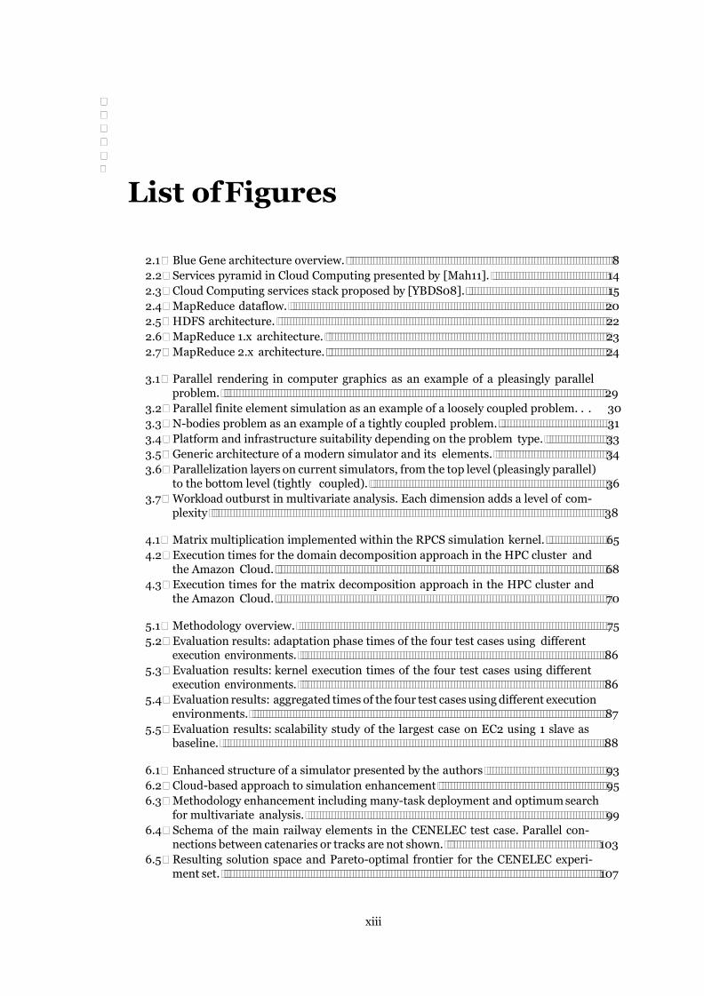
2.1 Blue Gene architecture overview. ......................................................................................... 8
2.2 Services pyramid in Cloud Computing presented by [Mah11]. ...................................... 14
2.3 Cloud Computing services stack proposed by [YBDS08]. ................................................ 15
2.4 MapReduce dataflow. .......................................................................................................... 20
2.5 HDFS architecture. .............................................................................................................. 22
2.6 MapReduce 1.x architecture. .............................................................................................. 23
2.7 MapReduce 2.x architecture. .............................................................................................. 24
3.1 Parallel rendering in computer graphics as an example of a pleasingly parallel problem. ............................................................................................................................... 29
3.2 Parallel finite element simulation as an example of a loosely coupled problem. . . 30
3.3 N-bodies problem as an example of a tightly coupled problem. .....................................31
3.4 Platform and infrastructure suitability depending on the problem type. .................... 33
3.5 Generic architecture of a modern simulator and its elements. ..................................... 34
3.6 Parallelization layers on current simulators, from the top level (pleasingly parallel) to the bottom level (tightly coupled). ............................................................................... 36
3.7 Workload outburst in multivariate analysis. Each dimension adds a level of com- plexity ................................................................................................................................... 38
4.1 Matrix multiplication implemented within the RPCS simulation kernel. .................... 65
4.2 Execution times for the domain decomposition approach in the HPC cluster and the Amazon Cloud. ............................................................................................................... 68
4.3 Execution times for the matrix decomposition approach in the HPC cluster and the Amazon Cloud. ............................................................................................................... 70
5.1 Methodology overview......................................................................................................... 75
5.2 Evaluation results: adaptation phase times of the four test cases using different execution environments. ..................................................................................................... 86
5.3 Evaluation results: kernel execution times of the four test cases using different execution environments. ..................................................................................................... 86
5.4 Evaluation results: aggregated times of the four test cases using different execution environments. ..................................................................................................................... 87
5.5 Evaluation results: scalability study of the largest case on EC2 using 1 slave as baseline. ............................................................................................................................... 88
6.1 Enhanced structure of a simulator presented by the authors ........................................ 93
6.2 Cloud-based approach to simulation enhancement ........................................................ 95
6.3 Methodology enhancement including many-task deployment and optimum search for multivariate analysis. .................................................................................................... 99
6.4 Schema of the main railway elements in the CENELEC test case. Parallel con- nections between catenaries or tracks are not shown. .................................................. 103
6.5 Resulting solution space and Pareto-optimal frontier for the CENELEC experi- ment set. .............................................................................................................................. 107
xiii

List of Figures xiv
6.6 Execution times for the enhanced methodology with increasing number of nodes and experiments. .............................................................................................................................. 108
6.7 Speed-up for the enhanced methodology, over one node. .............................................. 108
6.8 Efficiency of the enhanced methodology with increasing number of experiments. . 109

List of Tables
2.1 Top five positions in the Top500 ranking of November of 2015. ..................................... 10
2.2 Top five positions in the Graph500 ranking of November of 2015. ................................ 10
2.3 Top five positions in the Green500 ranking of November of 2015. ................................. 11
3.1 Characteristics of different parallelization layers in terms of computational resources. 39
3.2 Test cases definition .............................................................................................................. 45
3.3 Generic architectural concepts identified in RPCS and its domain characteristics. 46
4.1 Symbol table for the proposed communication and memory model .............................. 53
4.2 Execution profile of RPCS from gprof utility: top execution time functions list . 64
4.3 Node features for the HPC cluster and the Cloud used in the evaluation .................... 66
4.4 Test cases definition for the HPC-based approaches. ....................................................... 67
5.1 Examples of virtual cluster planning using different instance types, α = 30s and β = 1GB. .......................................................................................................................... 81
5.2 Job-specific configurations on MRv1 .................................................................................. 83
5.3 Job-specific configurations on MRv2 ........................................................................................... 83
5.4 Platform configuration parameters for MRv2 ................................................................... 83
5.5 Execution environments. ................................................................................................................. 84
5.6 EC2 instances description. ................................................................................................... 84
5.7 Test cases definition for the original vs. cloudified application ...................................... 85
5.8 Execution times per stage in minutes. Configurations and experiments defined in tables 5.5 and 5.7. ................................................................................................................. 88
6.1 Variations of electrical substations placement on MOO optimization ......................... 103
6.2 EC2 instances description. ................................................................................................. 106
6.3 Optimal configurations for each optimisation criteria for the CENELEC experi- ment set. ............................................................................................................................... 107
xv


Abbreviations
ANOVA ANalysis Of VAriance
ASCAC Advanced Scientific Computing Advisory Committee
BLAS Basic Linear Algebra Subprograms
CFD Computational Fluid Dynamics
DSM Direct Stiffness Method
DSP Digital Signal Processors
FEM Finite Element Method
FPGA Field-Programmable Gate Arrays
FSM Finite State Machine
GPGPU General Purpose Graphic Processing Unit
HPC High Performance Computing
IaaS Infrastructure as a Service
ISO International Organisation for Standardisation
IT Information Technologies
I/O Input / Output
LAPACK Linear Algebra PACKage
MNA Modified Nodal Analysis
MPI Message Passing Interface
MST Minimum Spanning Tree
NIST National Institute of Standards and Technology
OpenMP Open Multi-Processing
PaaS Platform as a Service
RPCS Railway Power Consumption Simulator
QoS Quality of Service
SaaS Software as a Service
ScaLAPACK Scalable Linear Algebra PACKage
SLA Service Level Agreement
TCO Total Cost of Ownership
UC3M University Carlos III of Madrid
XaaS Anything (X) as a Service
xvii


Chapter 1
Introduction
This chapter introduces the context of the work presented in this thesis. The first section provides
an overview on the main topics addressed in this thesis: simulation and Cloud Computing. The
second section presents a brief description of the motivation, and of the limitations of current
simulators to be addressed in this thesis. The next section discusses the specific goals of the
thesis work. Finally, the chapter concludes providing an outline for the rest of this document.
1.1 Definition and Scope
During the last years, simulation has become the way to research and develop new scientific
and engineering solutions in several areas [Ban98]. Simulation allows to reduce time and effort
invested in testing new engineering structures, molecular designs, climatic conditions, etc. The
ASCAC summary report [ABC+10] illustrates how simulation is used in leading science domains
like aerospace industry, astrophysics, etc., and Maceri and Casciati [MC03] enumerate uses of
simulation in civil engineering. Nevertheless, using simulators in developing science and engi-
neering solutions requires to face several challenges. Some of these challenges are inherent to
the simulation act: to develop a model that matches with the real system simulated, validate it,
and extrapolate the results to the real world. Ho et al. [HMY+02] illustrates these challenges
when developing simulation models for railway applications. However, some other challenges are
related to the complexity and scalability of the simulators. These challenges go further than the
simulator itself and impact on the relaying IT infrastructure.
One way to classify simulators is according to the infrastructure required to run a simulation (i.e.
how much resources and time are needed to run a simulation). In terms of computing power, or
memory consumption, some simulators require no more than a desktop computer or workstation
[SGG+12], while others require the use of hundreds of nodes [CHA+11]. Also, the most of the
simulators are tied to a specific platform, so small simulators are generally desktop applications,
while the most resource-demanding simulators are MPI programs, which need to be deployed in
HPC environments like clusters or supercomputers. There are few simulators relaying on cloud
environments [YCD+11].
1

Chapter 1. Introduction 2
Cloud computing is a relatively fresh term which has become in one of the most popular of
those related with IT. Cloud computing is defined by the NIST [MG09] as ”a model for enabling
ubiquitous, convenient, on-demand network access to a shared pool of configurable computing
resources (i.e., networks, servers, storage, applications, and services) that can be rapidly provi-
sioned and released with minimal management effort or service provider interaction”. In practice,
an institution (e.g. an enterprise or university) could have its own datacenter to perform tasks,
so it must carry with the respective management and maintenance. Other way is to outsource
the IT infrastructure to cloud providers. Then, management and maintenance task are less
demanding. A third option is the use of hybrid clouds, in which the institution has a private
infrastructure and outsources more computing power to a cloud provider when the workload
exceeds the available capacity.
With the explosion of cloud services and the Anything as a Service (XaaS) paradigm, cloud
service providers have started to offer several HPC paradigms as cloud services [APK+12]. Ex-
amples of this are MapReduce [Ama], MPI implementations [RBA11], and GPGPU processing
[ECW10]. In such cases, the client can resize the infrastructure according to the workload,
and saves the costs associated to management and maintenance. On the other hand, the client
must take a performance loss in comparison to bare metal executions. This loss comes from
several factors: the virtualization layer, which adds a little overhead to the applications, but
more importantly, the network latencies. Cloud infrastructures are associated to high network
latencies due to the fact that virtual machines can be placed anywhere in the cloud data center
(or even in different data centers). Besides, it is difficult for the applications to perform low level
optimizations (e.g. topology optimizations) because the underlying infrastructure is hidden.
Those simulators which run on HPC environments will likely benefit from these upcoming cloud
paradigms, but this migration should be analysed carefully. In this thesis, the use of simulators
both in HPC environments and the Cloud is addressed.
1.2 Motivation
The widespread use of simulators as a means of research and development in many fields has
made it necessary to run the largest number of simulations in the lowest time possible [CBP00].
Moreover, the need of processing or storing data has been increased significantly as the simula-
tions become more and more complex [LCL+09]. Furthermore, if it is desired to study variations
of multiple variables involved in the experiment, a single simulation is not enough to get relevant
results. Therefore, the use of simulators is limited by the availability of computing infrastruc-
tures (data centres, supercomputers, clusters, etc.) which have the required power to run the
simulations. In this context the use of HPC, both infrastructures (clusters, supercomputers) and
technologies (MPI, OpenMP, GPGPUs) is the major trend in simulation [ABC+10].
While these approaches have proved successful, they often rely on heavy hardware investment
and they are tightly conditioned by its capabilities and, more importantly, its availability, which
de facto limits actual scalability and the addressable simulation size. Since sharing resources
across multiple clusters implies several limitations, cluster applications cannot be considered

Chapter 1. Introduction 3
sustainable, because their scalability is strongly dependant on the cluster size. There are several
issues that can be tackled in order to develop a sustainable application, such as:
• Suitability. The way an application uses computational resources, such as CPU, memory,
and network, determines the performance of this application when it is executed on such
different infrastructures like HPC clusters and clouds. Therefore, this usage should be
analysed in order to establish under what kind of infrastructure an application will be
sustainable. For instance, if a a particular problem’s characteristics determine that it is
necessary a huge amount of network communications, ultimately this resource determines
the suitability of one kind of infrastructure (in this case a cluster) over the other (the
cloud).This analysis should start from the applications problem domain, checking resource
usage as the problem size becomes bigger and bigger.
• Independence. Making the application cloud/cluster independent, so that it can be de-
ployed in either of them with minimal changes. In this way, computational resources,
possibly located in different places, can be aggregated and local data center size would not
be a limitation. Moreover, HPC and cloud resources could be exploited simultaneously
following a hybrid scheme. Note that this issue clashes with the previous one.
• Scalability. Improving applications scalability by adapting them to the underlying infras-
tructure. In connection with the previous issue, clearly cloud infrastructures juxtapose
several characteristics (flexibility and scalability) to traditional HPC environments (bare
metal or topology optimizations, and low-latency networks), so the application should take
the best from each kind of infrastructure. This would minimize the added overhead of
working with more nodes, making a better use of the available resources.
• Flexibility. Making applications and infrastructures more flexible, bringing the possibility
of scale up or down according to instantaneous user needs. This is an inherent charac-
teristic of Cloud Computing infrastructures, and therefore it should be exploited by the
applications. Computing resources could be fitted to specific simulation sizes and deadlines.
As the Cloud Computing paradigm gains more popularity, the more services are deployed in the
cloud. The NIST definition of Cloud Computing also provides a description of three basic service
models: IaaS, PaaS, and SaaS [MG09], but nowadays these service models have been extended to
higher levels of abstraction (e.g. Database as a Service [HIM02, CJP+11], Network as a Service
[CMPW12]) which as a whole provide an Anything as a Service vision (XaaS). Simulation is not
aware of this trend, and there are current efforts to deploy simulation services on the cloud, like
[AM13] and [Xia11].
Using Cloud Computing in simulation provides several advantages related with the elastic nature
of the cloud. The infrastructure can be resized according to the number and complexity of the
simulations, and there is a variety of platforms and services in which simulators could rely
on. Along with its so-called pay-as-you-go model, allow to adjust the required instances to the
particular test case size while cutting-down the resulting costs. It would enable the execution of
large simulations with virtual hardware properly tailored to fit specific use cases like memory-
bound simulations, CPU-dependant computations or data-intensive analysis.

Chapter 1. Introduction 4
But there is also a number of challenges that must be faced up. The Magellan Final Report
[YCD+11] exposes these challenges, and some of them are stated here:
• There is an overhead for scientific applications executed on the cloud associated to the
absence of high-bandwidth, low-latency interconnects in virtual instances located (possibly)
on different places.
• The absence of high-performance file systems further impacts the productivity of running
scientific applications which perform intensive I/O within the cloud environment.
Given the former, this thesis suggests a methodology to transform the applications making
them both HPC and cloud suitable. The focus is on analysing the application problem domain,
getting the dependences of the application input data. On those loosely coupled sets of data this
thesis proposes a paradigm shift from classic parallel computations to a data-centric model that
would distribute the simulation load across a set of independent instances in a cloud suitable
manner. On those tightly coupled, backward compatibility is maintained on HPC programming
paradigms, taking advantage of HPC features (if available).
This thesis focuses on resource-intensive parallel simulations which hold potential scalability
issues on large cases, since cluster hardware may not satisfy simulation requirements under such
stress circumstances, and therefore will likely benefit from Cloud Computing paradigm. A case
study illustrating the whole methodology by means of a particular problem domain is provided:
simulation of time-variant electric circuits using the modified nodal analysis (MNA) technique.
The aim is to extend this problem to a general kind of scientific and engineering problems.
1.3 Objectives
The major goal of this thesis is to analyze the suitability of executing parallel simulations in
clouds by performing a paradigm shift, from classic parallel approaches to data-centric models,
in those applications where that is possible. The aim is to maintain the scalability achieved in
traditional HPC infrastructures, while taking advantage of Cloud Computing paradigm features.
This allows us to perform simulations on the Cloud, resizing the infrastructure and dynamically
balancing the workload according to the number and complexity of the simulations, but also
keeping HPC technologies such as MPI, for those cases which getting data independence across
the problem domain is not possible (i.e. they implement heavy communication patterns). By
exploiting the data-centric paradigm, a virtually infinite scalability is achieved, so that large
simulations can be executed independently of the underlying hardware resource, allowing us
to spread simulation scenarios of different sizes in a more flexible way, using heterogeneous
hardware, and taking advantage of shared inter-domain infrastructures. By maintaining HPC
technologies those heavy-coupled problems not suitable to the data-centric approach can be
tackled.
This goal can be split in the following ones:

Chapter 1. Introduction 5
O1 To explore the characteristics that make simulators suitable or unsuitable to be deployed on
HPC or Cloud infrastructures.
O2 To propose a methodology to adapt scientific parallels simulations following a cloud-suitable
data-centric scheme, while maintaining classic approaches to domain decomposition for
those problems which cannot be split gracefully.
O3 To transform a memory-bound simulator into the proposed scheme, integrating the original
application with both the MapReduce framework and MPI libraries.
O4 To demonstrate the feasibility of the resulting architecture comparing the behavior and
efficiency of adapted vs. original applications in both HPC and cloud environments.
O5 To enhance the proposed methodology in order to include multivariate analysis simulations,
as a particular case that can benefit from a cloud-suitable data-centric scheme.
With the study and analysis of the aforementioned objectives, the following contributions are
foreseen:
C1 Classification of simulation problems according to its suitability to HPC and cloud infras-
tructures and the different ways of parallelizing such problems.
C2 Proposition of different mechanisms to split simulation domains in smaller sub-domains,
with different degrees of data coupling, thus indicating the suitability of the simulator
to different infrastructures, identifying architectural bottlenecks, and those aspects which
limit the scalability of the application.
C3 Definition of a software framework suitable for both cloud and HPC systems, that makes
use of data-centric schemes such as MapReduce.
C4 Implementation of the mechanisms and frameworks proposed in a simulator, and perfor-
mance study when different computing resources (i.e. HPC and cloud) are used.
1.4 Structure and Contents
This document describes the work developed in this thesis. It has been organized into seven
chapters, whose contents are summarized in the following paragraphs:
• Chapter 1 introduces the scope and the motivation for this thesis. Analyzing the suitability
of performing simulations in Cloud by performing a paradigm shift is stated as the main
goal.
• Chapter 2 describes the state of the art in HPC, Cloud Computing, MapReduce, and the
current approaches to migrate scientific simulations to the Cloud.
• Chapter 3 contains the problem statement. A classification of simulation problems is
proposed, and an illustrative example of a simulation problem is analysed and modelled,
indicating all problem dimensions and their impact on the resource usage.

Chapter 1. Introduction 6
• Chapter 4 explores HPC-based approaches to decompose the problem, analysing their
suitability and performance with regard to HPC and Cloud infrastructures.
• Chapter 5 describes the proposed methodology to migrate the application to the cloud,
including all its phases, and providing an illustrative example of migration.
• Chapter 6 analyses the opportunities of the resulting architecture in multidimensional
analysis of simulation problems, where there is a high degree of data decoupling.
• Chapter 7 presents the conclusions, describes the future research lines, and the contribu-
tions of this thesis.

Chapter 2
State of the Art
This chapter provides a detailed State of the Art in both High-Performance-Computing and
Cloud Computing, which are the major trends used nowadays in simulation. In both cases
current technologies and paradigms used are described, as well as current challenges which have
to be tacked. Finally, a detailed analysis of the Hadoop MapReduce framework and its derived
projects is also provided, indicating its architecture and components.
2.1 High-Performance Computing
The term High-Performance Computing refers to the application of aggregated computing re-
sources and parallel processing algorithms and techniques to solve complex computational prob-
lems or analyse large amounts of data. Its applications are specially focused in scientific mod-
elling, simulations and analysis, which tend to involve large amounts of data and sophisticated
algorithms. Its main goal is to solve such problems in the minimum possible time, hence super-
computers tend to be composed of multiple interconnected nodes to increase concurrency.
2.1.1 HPC Infrastructure Elements
Supercomputers have many different architectures [Buy99], but share some common elements.
Supercomputers are composed of hundred of thousands of compute nodes which perform the
processing workload associated to a particular computational problem. A compute node is
composed of one or several cores which share a main memory following a shared memory building
blocks pattern [BKK+09]. The workload is distributed among as many as possible cores in order
to increase the parallelism and reduce the total execution time. Compute nodes are linked with
high-performance compute networks in order to share all data necessary to perform the
calculations. Such networks are deployed following complex topologies, such as mesh, hypercube,
or 3D torus [AK11]. The aim is to minimize communication delays between compute nodes
maximizing the CPU usage.
7


Chapter 2. State of the Art 9
National Laboratory, and Open MPI [GFB+04] developed by a consortium of academic,
research, and industry partners.
OpenMP Open Multi-Processing is an extension to the programming languages C/C++ and
Fortran, based on compiler directives [Boa13]. OpenMP provides automatic parallelization
of loops by adding compiler directives to the loop declaration. The compiler interprets the
directive and divides the loop task between several threads, so that the computational effort
is divided among multiple cores. The main advantage of OpenMP is the reduced impact
on the application source code, thus allowing to parallelize an application just adding a
few lines of code. Due to the fact that MPI provides distributed memory parallelism,
and OpenMP provides shared memory parallelism, they are used together frequently when
programming massively parallel applications [RHJ09, SJF+10]. MPI distributes the effort
between compute nodes, while OpenMP distributes the effort between cores of the same
node.
GPGPUs During the last years the use of General-Purpose-Graphic-Processing-Units as a
means to perform compute work offloading the CPUs have become widespread. GPG-
PUs evolve from the traditional video games graphic cards to generic devices capable of
performing a huge number of parallel arithmetical operations. The main advantage is the
high level of parallelism achieved by these devices, but as main drawback, these devices are
difficult to handle by programmers, requiring specific libraries and code for each concrete
kind of device [OHL+08]. The following list describes current technologies used to program
GPGPUs
CUDA Platform developed by Nvida with the aim of exploiting processing power of its
GPUs [NVI11]. CUDA provides C and C++ extensions, plus a mathematical library
specifically optimized to be executed on Nvida cards. While Nvida are the most pop-
ular GPGPUs in supercomputing, AMD and Intel have developed its own alternatives
to Nvida GPGPUS: AMD APP, and Xeon Phi respectively.
OpenCL OpenCL is the open counterpart of proprietary GPGPU programming platforms
[TNI+10]. OpenCL provides a programming language and API which creates data-
level parallelism thus allowing to offload compute tasks onto heterogeneous platforms
like CPUs, GPUs, digital signal processors (DSPs) and field-programmable gate arrays
(FPGAs). Currently, all GPGPU developers support OpenCL on its devices.
OpenACC OpenACC [Ope11] is a collection of compiler directives, similar to those uti-
lized in OpenMP, which can be used to perform parallel calculations on the CPU as
well as to offload compute task onto GPGPU devices. As OpenMP, OpenACC allows
to parallelize applications using these hardware devices with a minimum impact on
the source code. Besides, OpenACC provides portability across multiple GPGPUs
from different providers.
2.1.3 Current Supercomputers and Petascale Systems
Complex resource-intensive applications have traditionally found in high performance infrastruc-
tures the necessary hardware to fit their high-end needs. Supercomputers constitute a canonical

Chapter 2. State of the Art 10
sample of systems that are designed to achieve the highest number of floating-point operations
per second (FLOPS )[KT11]. HPC clusters and grids result from the association of a set of super-
computers under the same local network or across several administratively distributed systems,
respectively; they can also be heterogeneous and, as previously mentioned, gather both CPU
and GPU nodes [KES+09, FQKYS04].
Current leading systems in the Top500 rank [DMS+97] are GPU-based and capable of reporting
over one quadrillion flops (a petaflop) under the standardised Linpack benchmark [DL11]. Some
examples of the so-called petascale infrastructure are shown in Table 2.1, which includes the top
five positions in the Top500 ranking of November 2015 [DMS+97].
System Performance (Pflop/s) Power (MW) Location
Tianhe-2 33.86 17.81 China
Titan 17.59 8.21 USA
Sequoia 17.17 7.89 USA
K-Computer 10.51 12.66 Japan
Mira 8.59 3.95 USA
Table 2.1: Top five positions in the Top500 ranking of November of 2015.
Despite performance is a proper quantitative measure of an HPC system’s quality, researchers,
developers and end-users are increasingly aware of other critical characteristics that must be
considered in order to show the actual capabilities of the tested system for the efficient execution
of 3D simulations and analytics workflows, while minimizing computing cost.
The Graph500 rank [MWBA10] includes shared-memory, distributed memory and cloud bench-
marks for large scale graph-oriented algorithms. Its goal is to evaluate HPC system’s behaviour
when approaching complex data-intensive applications, measured in traversed edges per second
(TEPS ). Current leading positions in the November of 2015 Graph500 ranking are shown in
Table 2.2 [Top15].
System Performance (TTEPS) Location
K-Computer 38.62 Japan
Sequoia 23.75 USA
Mira 14.98 USA
JUQUEEN 5.84 Germany
Fermi 2.57 Italy
Table 2.2: Top five positions in the Graph500 ranking of November of 2015.
2.1.4 Future Goals: Green HPC, Exascale Infrastructures, and Big
Data
Nowadays, sustainability and energy efficiency is key in the development and evaluation of HPC
infrastructures. Following the Top500 philosophy, the Green500 list [FC07] is dedicated to rank
supercomputers, but in terms of their efficiency, which is measured in performance-per-Watt.

Chapter 2. State of the Art 11
Table 2.3 shows that current leading positions in the rank do not match any of the Top500
systems [Gre15], and their total power consumption is significantly less that the shown by the
latter. This indicates that there is still a lot of research to be done in order to reduce the
gap between performance and efficiency, especially considering that supercomputers will keep
increasing their target performance to reach the exascale goal [SSSF13].
System Performance (Mflops/W)
Power (kW)
Location
Shoubu -ExaScaler- 7031.6 50.32 RIKEN - Japan
TSUBAME-KFC/DL 5331.8 51.13 GSIC Center - Japan
ASUS ESC4000 5271.8 57.15 GSI Helmholtz Center - Germany
Sugon Cluster 4778.4 65.00 Institute of Modern Physics - China
XStream 4112.1 190.00 Stanford RCC - US
Table 2.3: Top five positions in the Green500 ranking of November of 2015.
Exascale systems will become the next generation of supercomputers, capable of performing with
at least one exaflop. Scientific simulations will likely benefit from the upcoming exascale infras-
tructures [ABC+10], however many challenges must be overcome [BBC+08, GL09] including,
processing speed [Cou13], data locality and power consumption; among them, energy efficiency
seems to be the most limiting factor [Hem10].
Nowadays, cheaper and lower power alternatives are on research to overcome such difficulties. For
instance, low-end processors are being considered to build large scale supercomputers. Besides,
multiple efforts are currently under way in order to reduce energy consumption without reducing
compute power, from scaling dynamically the number of compute cores [FL05], to deploy power-
aware techniques in the I/O subsystem [LBIC13].
Big Data [MCB+11] is a term closely related to exascale systems, and one of the challenges
that must be overcome. Big Data refers to the task of dealing with huge data sets, processing,
analyzing, and storing vast amounts of information. Big Data challenge arises as a result of data
explosion in society: web traffic, social networks, sensors, and pervasive or ubiquitous computing.
Present information systems do not achieve nowadays the required capacity to deal with all data
generated by current society. Besides, unpredictable events may lead to data explosions (see
[GALM07]), so it is required an elastic dimensioning of compute and storage infrastructures in
order to adapt system’s capacity to service demand.
2.2 Cloud Computing
Cloud Computing appeared as a cheaper, elastic possibility to achieve the ideal situation of
unlimited sustainable scalability. Cloud Computing is a popular paradigm that relies on resource
sharing and virtualization to provide the end user with a transparent scalable system that can
be expanded or reduced on-the-fly.
There were many definitions of ”Cloud Computing”. The NIST provided its own[MG09], which
was considered the most relevant: Cloud computing is a model for enabling ubiquitous, conve-
nient, on-demand network access to a shared pool of configurable computing resources (...) that

Chapter 2. State of the Art 12
can be rapidly provisioned and released with minimal management effort or service provider in-
teraction. The International Organisation for Standardisation (ISO) have adopted this definition
[ISO14] and now is a standard. Nevertheless, other definitions are listed by [VRMCL08], which
include the concepts of virtualization, web-based services, and user-friendly among others. Sev-
eral efforts have been carried out in order to standardize terminology and concepts of Cloud
Computing. [RCL09] proposes a taxonomy of Cloud Computing systems, and performs a survey
of Cloud Computing service providers, and [YBDS08] defines an ontology of Cloud Computing.
The NIST states five essential characteristics of Cloud Computing which are listed below (short-
ened):
On-demand self-service A consumer can unilaterally provision computing capabilities, with-
out requiring human interaction.
Broad network access These capabilities are available over the network, and accessed through
standard mechanisms.
Rapid elasticity These capabilities can be elastically provisioned and released, to scale rapidly
outward and inward commensurate with demand. To the consumer, the capabilities avail-
able for provisioning often appear to be unlimited.
Resource pooling The provider’s computing resources are pooled to serve multiple consumers
using a multi-tenant model, with different physical and virtual resources dynamically as-
signed and reassigned according to consumer demand. There is a sense of location indepen-
dence in that the customer generally has no control or knowledge over the exact location of
the provided resources but may be able to specify location at a higher level of abstraction.
Measured service Cloud systems automatically control and optimize resource use by leverag-
ing a metering capability at some level of abstraction appropriate to the type of service.
Cloud providers operate at several levels of virtualization, which are known as service models.
The NIST definition of Cloud Computing provides also a description of the three basic service
models: Infrastructure as a Service, Platform as a Service, and Software as a Service. But as
Cloud Computing services have become more popular, different authors have coined specific
specific service models as a characterization of one of the three basic aforementioned services.
For instance, [ZZZQ10] proposes three additional service models: Network as a Service (NaaS),
Identity and Policy Management as a Service (IPMaaS), and Data as a Service (DaaS). The
following subsections show a brief survey of the three basic service models and those derived
from them.
2.2.1 Infrastructure as a Service
In this model, providers offer physical or virtual resources like instances of raw virtual ma-
chines, block storage, virtual networks and disk imaging. The consumer is able to deploy and
run arbitrary software, which can include operating systems and applications. The consumer
does not manage or control the underlying cloud infrastructure but has control over operating

Chapter 2. State of the Art 13
systems, storage, and deployed applications; and possibly limited control of selected networking
components (e.g., host firewalls).
In [PO09], a taxonomy of this service model is proposed. IaaS clients can configure Virtual
Dedicated Servers (VDS), also called instances in Amazon WS terminology. These VDS are
virtual machines which can be customized by the user through deploying on top his/her own
OS and software. Besides, in order to ease servers deployment, most of IaaS providers supply
pre-configured generic VDS images. A number of images of a particular VDS can be deployed as
separate independent machines. Each one of these images can be allocated in different availability
zones: distinct locations (presumably distinct data centres) that are engineered to be decoupled
from failures in other zones.
The hardware settings of these images are based on three kinds of resources: compute units,
memory, and hard disk. A compute unit is an abstract term which defines the processing power
of the machine. Theoretically, one compute unit is equivalent to one core, but the clock speed
and the concrete core architecture is not always specified, and varies between different providers.
The memory indicates the RAM size of the image, while the disk indicates the number and
capacity of volatile disks (i.e. cleaned up after image termination).
Finally, most of IaaS providers offer additional services with regard to VDS administration and
management. The following list describes the most regular:
Load balancing Refers to spreading a service workload between two or more VDS in order to
avoid overloaded servers.
Resizing Adjustment of the amount of resources provisioned to an VDS based on the exhibited
load. More compute unit, memory or disk can be added dynamically.
Checkpointing Refers to the capability of saving a snapshot of the running VDS (including all
applications, data, conguration les, etc.) at any time instance.
The Cloud360 website [Clo14] provides a list of the top 20 IaaS providers. Amazon WS leads
the list as the world’s most important provider. Amazon EC2 sets the standard for spinning up
and taking down cloud capacity. AT&T follows, offering Compute as a Service and Storage as a
Service with SLA of 99.99 percent availability.
2.2.2 Platform as a Service
This model provides a full computing environment in which developers can create their own
applications without having to concern themselves with hardware infrastructure. The capability
provided to the consumer is to deploy onto the cloud infrastructure consumer-created or acquired
applications, while the provider supplies programming frameworks, libraries, services or tools.
This allows developers to have access to a wide range of licensed software ready to create or
deploy their applications, without managing the underlying hardware. For instance, a provider
may offer a database platform where the PaaS user can deploy his/her own relational model.


Chapter 2. State of the Art 16
Several works have tackled the challenge of migrating scientific simulations to the cloud. A
discussion about the use of clouds in science is conducted on [Lee10], where benefits and issues
are analysed. [TLSS11] proposes SimSaaS (Simulation Software as a Service), a framework that
combines a cloud multi-tenant architecture with simulation software, strongly focusing on data
isolation and security. This framework is an evolution a service-oriented architecture proposed
by the same author in [TFCP06].
2.2.5 Current Challenges in Cloud Computing
Cloud Computing is nowadays a widespread model used by enterprises all over the world. Nev-
ertheless, this business model is still considered far from reaching maturity. Gartner’s hype cycle
of Cloud Computing [Smi12] still places most of the cloud key concepts far from the plateau of
productivity. Besides, a survey carried out by Cloud Security Alliance [CSA12] finds that cloud
market has not yet reached a level of maturity that will support major industry disruptions.
Survey participants believe that platform and infrastructure service offerings are still in the in-
fancy stage of maturity, while software service offerings are just emerging from infancy and are
in the early stages of market growth.
There are still many challenges to be overcome in order to consider Cloud Computing as a
completely mature technology. The following list provides a brief description of these challenges,
obtained from several sources:
Security and privacy in clouds Data security and privacy in clouds is the main issue that
concerns potential users of Cloud Computing [AFG+10, DWC10]. Following the service
models, cloud users are placing his/her data onto the provider’s infrastructure, which
represents a security issue due to intentional or non-intentional provider’s malpractices.
This security issue can be analysed from several perspectives:
1. Companies are reluctant to give its sensible data to third-party enterprises which
could access and use, (or sell) this information to external agents. Otherwise, failures
in providers security infrastructure may lead to involuntary data leaks. Recent NSA
scandal has situated the focus on this particular aspect [Art13].
2. Companies are concerned about whether its services or data will have the required
availability. Provider infrastructure failures have a direct impact on the client, and
may lead to services interruption or data loss [Cla12].
3. Virtualization technologies used in Cloud Computing difficult the traceability and
auditability of applications and data. Security records may expire when virtual ma-
chines are terminated. Besides, as long as many parties are involved on a cloud service
delivery (cloud user, cloud provider, third-party vendors, etc.), it is difficult to provide
consistent logging across all these parties.
Finally, the concept of ”reputation fate-sharing” has arisen between companies which use
cloud services [AFG+10]. One costumer’s bad behaviour can affect the reputation of others
using the same cloud, since all customers are sharing the same computational resources
(network addresses, physical machines, etc.).

Chapter 2. State of the Art 17
Portability and interoperability One of the current issues in Cloud Computing is the ab-
sence of a common specification of Cloud services. An early stage of maturity in this
industry leads to absence of standards and fierce competition in order to get dominance
in markets. Practically every cloud provider offers a custom API to access its services,
implementing different interfaces and behaviours. As a result, portability and interoper-
ability between different cloud providers gets hard, since potential clients who want to
interoperate with several providers have to implement several of these interfaces and be-
haviours. Besides, one of the main issues in cloud industry is the so-called ”vendor lock-in”,
in which cloud clients get tied to its providers due to the high costs of re-implementing its
applications adapting them to APIs of another providers.
There are several scenarios in which the use of multiple clouds is desirable: guarantee
performance or availability, change of cloud vendors, or distribute a deployment across
federated or hybrid clouds. Petcu et al. [Pet11, PMPC13] enumerates a list of requirements
which have to be accomplished before performing cloud interoperability with an acceptable
chance of success. Some of them are stated below:
1. At programming level, moving from one provider to another shouldn’t imply a dra-
matic reimplementation. This can be reached through the existence of a common
set of interfaces which would allow to manage simultaneously clouds from different
providers. Besides, a common ontology of cloud computing is necessary in order to
standardize components and behaviours, which may vary across different providers.
With regard to this requirement, currently small cloud providers tend to implement
the most popular APIs even if they are property of a competitor. For instance, Open-
Stack implements the Amazon AWS interface in order to attract Amazon clients. This
may lead to a de facto standardization of APIs of the strongest providers.
2. At application level, the ability of spanning multiple cloud services should be per-
formed in a transparent fashions. Examples of this could be moving data across dif-
ferent clouds or allocate computing resources on public clouds when a private cloud
application hasn’t enough available resources on its private cloud.
3. At monitoring level, SLA and performance monitoring should be delivered in an ho-
mogeneous and standardized fashion. This imply the creation of a set of benchmarks
to evaluate performance factors, equivalent to all providers, as well as a common
interface for supporting monitoring and management of load balanced applications.
Besides, equivalent SLA metrics should be established between all providers in order
to compare the quality of delivered services.
4. At deployment level, the ability to allocate resources from multiple cloud services
should be managed with a single tool, in order to ease application deployment, config-
uration and management. Common platforms should be provided, in order to ensure
that users can navigate between services/applications, enabling that a service hosted
on one platform could automatically call another service hosted by other platform.
5. At authentication and security level, single sign-on for users accessing multiple clouds
would be necessary, as well as integration of different security technologies, in order
to provide an holistic vision of the security architecture, shared by all participants in
the cloud service delivery (consumer, provider, third-party vendors, etc.).
Chapter 2. State of the Art 18
Energy issues Energy efficiency is a major concern in current ICT, as well as one of the major
challenges that must be overcome in order to achieve Exascale systems. Cloud Computing
is not aware of this trend, so efforts are under way to increase energy efficiency in data
centres, (i.e. decreasing power consumption while maintaining SLAs). As it is stated
in [BGDG+10], energy-related costs amount to 42% of the Amazon data centre TCO,
including both direct power consumption (19%) and the cooling infrastructure (23%).
Several techniques to improve energy efficiency in data centres have been already developed
and deployed, and several others are under research. The following list describes briefly
some of them:
1. Energy-efficient hardware. This approach is focused on developing hardware (CPUs,
motherboards, disks) that consumes much less energy. Computer power can be saved
by means of various well-known techniques, such as power down the CPU or switch
off disks if there isn’t any I/O activity.
2. Energy-aware scheduling in MP systems. These techniques schedule workload on a
data centre trying to optimize power consumption across the servers. Tasks with
different characteristics (compute bound, memory bound, I/O intensive) may have
different footprint on server consumption. Moreover, virtualization may be used to
consolidate several (virtual) servers in only one physical server.
3. Power minimization in clusters of servers. This technique is based on maintaining
active a small set of active servers, while other servers are down to a low-power state.
Due to the time required to turn up servers, it is necessary to foresee data centre
utilization and keep a number of servers ready to face unexpected peak demands.
2.2.6 Trends in Cloud Migration and Adaptation Techniques
As already mentioned, scientific applications and their adaptability to new computing paradigms
like the Cloud have been dragging increasing attention from the scientific community in the last
few years.
The possibility to run simulations in the Cloud in terms of cost and performance was studied
in [JDV+09], concluding that performance in the Abe HPC cluster and Amazon EC2 is similar
–besides the virtualization overhead and high-speed connectivity loss in the cloud– and that
clouds are a viable alternative for scientific applications. Hill [HH09] investigated the trade-
off between the resulting performance and achieved scalability on the cloud versus commodity
clusters; despite at the time of this work the Cloud could not properly compete against HPC
clusters, its low maintenance and cost made it a viable option for small scale clusters with
a minimum performance loss. Amazon [PBB15] proposes migrating HPC applications to its
Cloud, but (surreptitiously) establishes restrictions to the size of the virtual cluster in those
applications which are tightly coupled.
In this context, trends are naturally evolving to migrate applications to the Cloud by means
of several techniques, and this includes scientific simulations as well. D’Angelo [D’A11] de-
scribes a Simulation as a Service schema in which parallel and distributed simulations could be

Chapter 2. State of the Art 19
executed transparently, which requires dealing with model partitioning, data distribution and
synchronization. He concludes that the potential challenges concerning hardware, performance,
usability and cost that could arise could be overcome and optimized with the proper simulation
model partitioning.
In [SJV12], Srirama et al. study how some scientific algorithms could be adapted to the Cloud
by means of the Hadoop MapReduce framework. They establish a classification of algorithms
according to the structure of the MapReduce schema these would be transformed to and suggest
that not all of them would be optimally adapted by their selected MapReduce implementa-
tion, yet they would suit other similar platforms such as Twister or Spark. They focus on the
transformation of particular algorithms to MapReduce by redesigning the algorithms themselves.
Application adaptation middle-wares have also been developed to allow legacy code migration to
the Cloud. For instance, in [YWH+11] a virtualization architecture is implemented by means of
a Web interface and a Software as a Service market and development platform. This generalist
approach is suitable to provide multi-tenancy in desktop applications, but might not suffice for
the resource-intensive computations required by large-scale simulations.
Finally, in [SIJW13] there can be found interesting efforts to move desktop simulation applica-
tions to the Cloud via virtualized bundled images that run in a transparent multi-tenant fashion
from the end user’s point of view, while minimizing costs. However, the virtualization middle-
ware might affect performance since it does not take into account any structural characteristics of
the model, which could be exploited to minimize migration effects or drastically affect execution
times or resource consumption.
Despite Cloud Computing has proven itself useful for a wide range of scientific applications, its
utility for tightly-coupled HPC applications is still under research and development, mostly
because of the added communication overhead and the heterogeneous underlying hardware
[JRM+10]. Lately, several efforts have been made in the opposite direction: trying to adapt
HPC resources and infrastructures in order to offer a Cloud-fashioned interface, bringing elastic-
ity and pay-per-use model but avoiding the virtualization layer and maintaining the applications
close to the real hardware. An example of this trend is the solution provided by Penguin Com-
puting [Sch15], which offers a cloud service with bare-metal access, Infiniband interconnects, and
support by HPC experts.
2.3 MapReduce
As seen in the previous section, one of the promising models that has been increasingly considered
to adapt simulations to the Cloud is the MapReduce parallel computing framework, specially
in cases in which data locality is key to improve performance by reducing data transmission
overhead. The MapReduce paradigm [DG08] consists of two user-defined operations –map and
reduce– and three additional phases that handle the original data, the intermediate results and
the final output. Figure 2.4 shows the MapReduce dataflow and their stages, which behaves as
follows:


Chapter 2. State of the Art 21
supports automatic task execution plan optimizations, so that the developer does not have
to be tied to the classic MapReduce structure.
Hadoop MapReduce The most popular MapReduce implementation derived from the origi-
nal Google’s MapReduce and Google File System (GFS), providing an open-source alter-
native for both of them, is designed to be run on commodity hardware. Nowadays, Hadoop
MapReduce is executed on top of the Hadoop Distributed File System (HDFS), the Hadoop
Common platform and the Yet Another Resource Negotiator (YARN) resource manager,
while sharing this environment with other related projects such as HBase (database sys-
tem), Hive (data warehouse infrastructure) and Mahout (machine learning algorithms). It
was designed to deal automatically with failures in one or several nodes of the cluster, thus
resulting in a high-availability solution for data-processing infrastructures.
Spark This Hadoop-related project is focused on improving MapReduce’s deficient performance
regarding iterative jobs and interactive analytics [ZCF+10]. Examples of these uses cases
include parameter optimization on a static dataset, in which each iteration constitutes a
job, and queries on large partitioned datasets, requiring a job per query. Spark’s approach
is based on a read-only Resilient Distributed Dataset that can be loaded into memory across
many machines allowing multiple parallel operations on the same input data with no need
for intermediate writes. Furthermore, Spark is not tied to the MapReduce framework and
supports other programming models.
Elastic MapReduce Amazon’s Elastic MapReduce (EMR) is a web service dedicated to pro-
cess data on Hadoop MapReduce. It provides further advantages regarding multiple cluster
manipulation, virtual cluster on-the-fly resizing, Simple Storage Service (S3) integration
and HDFS support on local ephemeral storage.
Cloud MapReduce Similarly to EMR, this is another MapReduce implementation for the
Cloud built on top of Cloud OS, a resource manager for the set of machines integrated to
build the underlying cloud. Besides allowing incremental scalability and resizing, its most
interesting feature is its decentralized and symmetric architecture in which all the nodes
have the same responsibilities, even on heterogeneous environments [LO11].
2.3.1 Hadoop MapReduce
Apache Hadoop [Whi09] has been selected as main platform given its increasing popularity and
community support. Its distributed file system is a great addition to the framework, since it
allows automatic load balance and includes a distributed cache that supports auxiliary read-only
file storage for tasks among all nodes. Besides the former technical features, Hadoop has been
increasingly adopted into cloud environments along with other MapReduce frameworks, resulting
in reduced costs given its parallelism exploitation capabilities [KPP09].
In addition, studies regarding the relationship between the Cloud and Hadoop MapReduce for
scientific applications have established that performance and scalability results are similar be-
tween traditional clusters and virtualized infrastructures running this platform [GWQF10].


Chapter 2. State of the Art 25
2.4 Cloud Computing and Scientific Applications
Scientific applications and their adaptability to new computing paradigms have been dragging
increasing attention from the scientific community in the last few years. The applicability of the
MapReduce scheme for scientific analysis has been notably studied, specially for data-intensive
applications, resulting in an overall increased scalability for large data sets, even for tightly
coupled applications [EPF08].
Hadoop MapReduce is nowadays widely used as base platform for new programming languages
and architectures. Hadoop MapReduce is used in Pig Latin [ORS+08], an associative language
used in Yahoo for taking advantage of both declarative languages and map-reduce programming
style. This approach is strongly focused on processing data sets, and does not tackle the issue
of scientific workflows. Apache Hive [TSJ+10] and Bigtable [CDG+08] are two storage systems
developed on the top of Hadoop. Hive expresses data queries in an SQL-like declarative language
which is compiled into map-reduce jobs. Bigtable uses a sparse, distributed, multi-dimensional
sorted map to provide a fast method to access data, although de data structures exposed to the
user are rows, columns, and tables.
Nevertheless, the most popular evolution of Hadoop MapReduce is Spark [ZCF+10]. Spark
evolves the map-reduce programming style operating on resilient in-memory distributed data
sets, thus improving performance in workflows (since the data does not have to be written
to disk between tasks). Finally, an approach more related to scientific simulations is Twister
[ELZ+10], a runtime specifically designed for iterative map-reduce works and, therefore, more
suitable for repetitive computations over the same data.
The relationship between Apache Hadoop MapReduce and the cloud for scientific applications
has also been tackled in [GWQF10], which establishes that performance and scalability results are
similar between traditional clusters and virtualized infrastructures. In [SJV12], Srirama, Jakovits
and Vainikko study how some scientific algorithms could be adapted to the cloud by means of
the Hadoop MapReduce framework. They establish a classification of algorithms according to
the structure of the MapReduce schema these would be transformed to. They suggest that not
all of them would be optimally adapted by their selected MapReduce implementation, yet they
would suit other similar platforms such as Twister or Spark. They focus on the transformation
of particular algorithms to MapReduce by redesigning the algorithms themselves, and not by
wrapping them into a cloudification framework as this thesis proposes. A similar approach is
HAMA [SYK+10], a framework which provides matrix and graph computation primitives on the
top of MapReduce. An advantage of this framework over traditional MPI approaches to matrix
computations is the fault tolerance provided by the underlying Hadoop framework. Finally, an
approach for using Hadoop MapReduce in scientific workflows is that explained in [XZSA13],
whose authors propose a new architecture named SciFlow. This architecture consists on a new
layer added on the top of Hadoop, enhancing the patterns exposed by the framework with new
operations (join, merge, etc.). Scientific workflows are represented as a DAG composed of these
operations.
More related with the proposed approach is the so-called parameter sweep [CLZB00], in which
the same simulation kernel is executed multiple times with different input parameters, thus

Chapter 2. State of the Art 26
providing task independence. A related point of view is the many-task computing paradigm
[RFZ08], in which a high number of loosely coupled tasks are executed over data sets for a
short time. In this context, cloud computing has been proved as a good solution for scientists
who need resources instantly and temporarily for fulfilling their computing needs [IOY+11].
On the other hand, these evaluations show that better performance is needed for clouds to be
useful for daily scientific computing. SciCumulus [dOOBM10] is proposed as a lightweight cloud
middleware to explore many-task computing paradigm in scientific workflows. This middleware
includes a desktop layer to bring the scientist the possibility of composing their own workflows,
a distribution layer to schedule the flows in a distributed environment, and an execution layer
to manage the parallel execution of the tasks. The preliminary results demonstrate the viability
of the architecture.
2.5 Summary
In this chapter, the state of the art in HPC and Cloud Computing has been described. An
overview of the current state, trends, and application suitability for both paradigms has been
provided, pointing also the differences between them in terms of efficiency, elasticity, and adapt-
ability. A survey of Hadoop MapReduce, a popular platform designed to process big amounts
of data, that can be deployed on both HPC and Cloud infrastructures, has also been presented,
as well as a thorough research on those simulators or engineering applications that are currently
being migrated from HPC to Cloud, usually through MapReduce. These applications are very
demanding in terms of computing power and efficiency, and therefore their migration must be
studied carefully. In the next chapter the problem types that must be addressed in order to
migrate a simulator from HPC to Cloud environments are studied.

Chapter 3
Problem Statement
There is a huge catalogue of simulation problems associated to scientific and engineering domains,
but from the viewpoint of exploiting HPC and Cloud resources, it is meaningful to classify those
problems according to its suitability for each particular infrastructures. HPC resources, in general
terms, provide higher CPU power, on the basis of a similar number of computing resources such
as CPUs, nodes, and disks. This is due to several reasons:
• HPC infrastructures do not use a virtualization layer (or at least, not as thick as its cloud
counterparts) in order to detach the real hardware from the user point of view. And it is not
only the added overhead of the virtualization layer, but also the possible collision of different
users for the same hardware. In clouds, resources like processors or nodes are masked to
the user, and several users can share (unwittingly) the same node, interfering each others
in shared resources like cache memories, main buses, etc. Besides, the virtualization layer
hampers those architecture-specific optimizations which cannot be translated dynamically
at run time (e.g. SIMD instructions).
• HPC infrastructures are deployed using low-latency networks, specifically intended to de-
crease performance penalty in those problems which require a great amount of communi-
cations. Besides, all nodes in a cluster are held together arrayed in racks, the layout known
by the network stack, so optimizations in communications can be performed. While clouds
can perfectly deploy the same kind of networks, the virtualization layer, and the variable
allocation of virtual machines prevent the application from knowing the underlying topol-
ogy. Besides, cloud infrastructures can be spread across several data centres, which implies
the possible allocation of virtual machines far from each other.
• HPC infrastructures deploy parallel file system in order to manage massive I/O. Such
parallel file systems are hard to deploy in cloud infrastructures due to topology unawareness
and software/hardware decoupling. The same principle can be applied to tuned computing
libraries like 1ScaLAPACK, which usually are optimized for the underlying hardware.
1http://www.netlib.org/scalapack/
27

Chapter 3. Problem Statement 28
On the contrary, Cloud Computing paradigm provides with more elastic infrastructures. The
key feature of Cloud is that the user can size computing resources according to its particular
needs. This is particularly useful on simulation, where workloads are strongly dependent on the
size of the simulation, and the deadline the user wants to meet. Variable simulation sizes, or
urgent necessities for obtaining immediately results may lead to big differences in the computing
resources required.
Given the former, it is necessary to find how to make simulators suitable for both HPC and
Cloud Computing, considering these big differences between both models. The fist step towards
this direction is analysing and classifying problem types according to its suitability to these kinds
of platforms.
3.1 Problem Types
On analysing a problem suitability for HPC or Cloud infrastructures, data and communications
are the factors that have more relevance. There are two issues about data that should be
analysed: data quantity and data structure. Data quantity is relevant because of the economic
factor associated to Cloud Computing. Storing and processing information on the Cloud may
suppose an expense proportional to the amount of data processed and stored. While the key
advantage of Clouds is the elasticity of the infrastructure, the more resources you allocate,
the more costs you have to pay. Therefore big amounts of data imply big expenses. Data
structure is relevant because high latencies in clouds penalize applications which perform a lot of
communication. Therefore a parallel application which has to swap much data between compute
nodes in order to process the information (e.g. a parallel simulator performing a simulation),
will behave poorly on clouds.
Due to the fact that economic aspects of Cloud Computing exploitation fall out of the scope
of this thesis, the following analysis will be focused on data structure, classifying the problems
according to the structure and dependences between its data.
3.1.1 Pleasingly Parallel Problems
Pleasingly parallel problems (also called embarrassingly parallel problems) are those kind of
problems which are the easiest to implement in parallel. In pleasingly parallel problems the input
data set can be decomposed and processed in several independent tasks, with no communication
required between those tasks. Thus, the initial workload can be split among a number of compute
nodes, and each node can process its part of the data independently. Because no communication
is required between tasks, high network latencies have a minimal impact on performance (only
at the initial stage of distributing the workload). Therefore this kind of problems are the best
suitable for Cloud Computing, though they also perform well on HPC.
The following list contains several examples of pleasingly parallel problems:

Chapter 3. Problem Statement 29
Figure 3.1: Parallel rendering in computer graphics as an example of a pleasingly parallelproblem.2
• Distributed relational database queries. If a table is split among multiple nodes, each node
can process its own part of the table without interacting with other nodes, apart from
merging the results of all nodes on finalization.
• Fractals (e.g. Mandelbrot set). Each point of the set can be calculated independently,
so the problem domain (i.e. a set of complex numbers) can be split among the compute
nodes.
• Rendering of computer graphics. The same principle stated before applies to computer
graphics, in which each pixel of the screen can be rendered independently. Finally all
pixels are merged forming the final picture. Figure 3.1 illustrates an example of parallel
rendering in computer graphics.
• Matrix multiplication. On multiplying matrices AB = C. Each element cij of the resulting
matrix can be calculated using only i row from A and j column from B, so the workload of
calculating the resulting elements can be split across compute nodes, provided each node
has access to the corresponding rows and columns from A and B.
2http://www.kitware.com

Chapter 3. Problem Statement 30
Figure 3.2: Parallel finite element simulation as an example of a loosely coupled problem.3
3.1.2 Loosely Coupled Problems
In this type of problems, the problem domain can be decomposed easily in several subdomains.
but there is a (weak) dependence between those subdomains. They have to share information
with their neighbours, or they influence its neighbours somehow. A certain amount of commu-
nication between compute nodes is required in order to solve the problem in parallel. While the
boundaries of these communications are limited to a local scope, for instance adjacent CPUs in
the virtual topology (otherwise we would be talking about tightly coupled problems), the impact
of high latencies gets worse as the problem becomes bigger or it is required a higher degree of
accuracy in the simulation.
All problems which involve partial differential equations, such as FEM or CFD, are loosely
coupled problems. In such problems, the simulated structure/body/fluid is decomposed and
simulated in several independent pieces, but the iterations between those decomposed pieces
have to be calculated also in order to reflect a realistic behaviour (see Figure 3.2). Another
loosely coupled problem is a (parallel) convolution, in which two functions are compared across
the problem domain trying to find overlapped areas. One example of this would be a filter applied
to an image. The image can be decomposed in several pieces, so the filter is applied in parallel
to those pieces, but the boundaries between pieces have to be checked also, so a bordering region
should be shared between neighbours.
3.1.3 Tightly Coupled Problems
These problems are the hardest to implement in parallel. In tightly coupled problems, every
single entity (or most of the entities) of the problem domain has a certain amount of influence
on the others. Therefore, there is a strong dependence, and each partition of the problem needs
information of the others to solve the problem. A large amount of communications is required
3http://ccpforge.cse.rl.ac.uk/gf/project/parfel

Chapter 3. Problem Statement 31
Figure 3.3: N-bodies problem as an example of a tightly coupled problem.4
to solve this problem in parallel, and this amount is increased exponentially as the problem size
grows. Hence, communication latencies have a great impact on performance when solving this
kind of problems.
A classic example of a tightly coupled problem is the N-bodies problem. In the N-bodies problem,
the behaviour of a number of bodies have to be simulated, provided that each body interacts
with the others (see Figure 3.3). Examples of interactions are gravitational (each body attracts
and it is attracted by the others) or electromagnetic. Provided a domain decomposition based on
bodies (each node calculates and updates a subset of the total bodies), since every different body
influences all the others, some kind of information have to be exchanged between the nodes in an
all-to-all fashion. Another example of a tightly coupled problem is the parallel implementation
of Dijkstra’s Algorithm, in which each node tries to find the shortest path independently, but on
each interaction all results have to be merged in order to find what is the global shortest path.
3.1.4 Multivariate analysis: A Pleasingly Problem Particular Case
Simulators are widely used as tools not only for developing new designs or solutions, or im-
proving existing ones, but also as part of optimization processes, with the aim of exploring a
problem search space, trying to find the optimal components of a system. In other approaches,
it is required to understand the behaviour of the system in response to variations of the input
4http://parallel.massey.ac.nz/projects.html

Chapter 3. Problem Statement 32
parameters. These approaches are called multivariate analysis, in which the value of one pa-
rameter is adjusted by sweeping the parameter values through a user defined range, checking for
each value the behaviour of the system through simulation. Multivariate analysis usually implies
performing not one but many simulations, using the same simulator but varying the input data.
In this context, the whole task of exploring the problem’s search space obtaining the optimum
(or optimums, if performing a multi-objective optimization) can be considered as a pleasingly
parallel problem. Each single simulation is a sub-part of the a whole search problem. Apart
from scoring and comparing the solutions once simulated (which can be considered as a kind
of ”merge” operation), there are no dependences between simulations, and therefore they can
be executed independently. Note that this can be considered a pleasingly parallel problem
regardless of whether the simulation problem itself is a pleasingly parallel problem, a loosely
coupled problem, or a tightly coupled problem. In this case, there are two levels of parallelism:
• Data-level parallelism, based on the multiple independent simulations which can be per-
formed concurrently, each one of them with a different input.
• Task-level parallelism, if each one of those simulations can be performed in parallel (either
in a pleasingly parallel, loosely coupled, or tightly coupled fashion).
Examples of such kind of simulators can be found in [SGG+12] and [GGS+13]. These works
introduce a simulator that designs and calculates railway portal frames. The structural calcu-
lations of an structure are performed using the direct stiffness method (DSM) which can be
considered as task-level parallelism, but the tool also proposes different designs, looking for
the best-suited structure that fills some requirements, thus performing multiple calculations of
different structures, which can be considered as data-level parallelism.
3.1.5 Problem Types, Infrastructures and Platforms
Hadoop MapReduce have become in one of the most suited platforms for running applications
on the Cloud. In Section 2.3 the main characteristics and architecture of MapReduce are de-
tailed. As conclusions, it was stated that MapReduce uses data locality to improve performance,
reducing data transmission overhead. This makes MapReduce an ideal platform on those en-
vironments where a huge amount of distributing processing is required, and communication
latencies penalize the throughput according to amount of data transmitted through the network.
MapReduce is also suitable for cluster environments on those operations which can be adapted
to the map-reduce paradigm, yet it’s lack of flexibility makes it a secondary option, with MPI
performing the leading role.
As said in Section 2.1.2 MPI represents a standard de facto when developing HPC applications to
be executed on HPC environments. MPI low-level optimizations and topology awareness makes
MPI the best option on low-latency networks such as clusters or supercomputers. However,5MPI lacks of integrated fault-tolerance mechanisms for fault-tolerance and elasticity, as well as
5At least in the MPI specification document. Particular implementations may integrate non-standard mecha-
nisms


Chapter 3. Problem Statement 35
• Output data. The results obtained from the simulation. They must be stored in permanent
storage such as databases or data files.
• Multivariate analysis. The concept of performing multiple simulations, varying on each
one the input data set in order to obtain different results according to the variation. Op-
timization processes or ANOVAs are examples of multivariate analyses. A multivariate
analysis constitutes several of the processes depicted in Figure 3.5.
Secondly, more specific concepts are defined, restricted to the scope of this generic architecture:
• Modelling module. The module that receives the input data and translates such data into
the representation determined by the simulation model (matrices, graphs, etc.).
• Domain decomposition. The process of splitting the domain representation into smaller
parts. These parts may have a degree of dependence between them, depending on the
particular domain and simulation model. The more dependence, the more communication
will be required between subdomains to perform the simulation. Domain decomposition
is not strictly an essential element of common simulators, but should be present in those
simulators intended to perform on parallel high-end infrastructures.
• Subdomain. A division of the original domain that can be operated by the simulation
model independently (to a certain extent) from the others. Although, it may be necessary
to merge some data in order to complete the simulation.
• Simulation kernel. A set of mathematical operations that constitutes the mathematical
solver of the simulation model. Matrix operations and iterative processes (e.g. Newton-
Raphson or the conjugate gradient method) usually compose the simulation kernel of most
operations. [LKC+10] enumerates a list of popular simulation kernels along with its char-
acteristics in terms of resource usage, and opportunities for parallelization.
• Intermediate data. Many simulators generate intermediate data during the execution of
the simulation kernels on each of the subdomain partitions. These data may be too large
to be kept in memory and usually is sent to permanent storage on the last phase of the
simulation kernel. Later, these data may be merged in a final phase of the simulation, in
order to extract the definitive results.
Finally, some concepts that are present in a representative set of simulators but have not been
included in the architecture are listed, as well as the reasons for such decision:
• Data workflows. Some simulators are composed of several consecutive phases, in which
the output data of the previous phase is the input data of the next one. On each one of
these phases different operations are applied to the data, forming a bound graph. These
workflows are not represented on the proposed architecture, though they can be seen as
several different simulation kernels applied in sequence, thus applying the same techniques
taken to one simulation kernel.


Chapter 3. Problem Statement 37
in several subdomains, simulating each subdomain separately and finally recomposing the domain
again. Therefore another opportunity for paralelization can be found at this middle level, yet
this time it is possible that the resulting problem will not be a pleasingly parallel problem. The
kind of problem depends strongly on the particular domain characteristics. On FEM or CFD
problems, domain can be split with few dependences (only boundary conditions), thus resulting
in a loosely coupled problems. On other domains, pleasingly parallel or tightly coupled problems
may appear.
Finally, each one of the domain decomposition described before are usually translated to partial
differential equations or linear equation systems, and simulated through algebraic operations,
involving huge matrices (dense or sparse) that have to be added, multiplied or inverted. On
operating these huge matrices, lies another level of parallelism. Algebraic operations can be
operated in parallel, yet there is a strong dependence between the matrix elements, thus leading
to a tightly coupled problem. Parallel algebraic operations are usually conducted on clusters and
supercomputers, making use of specialized libraries such as BLAS and ScaLAPACK, optimized
for the underlying hardware.
These three levels can coexist in the same simulator. On making the decision of migrating a
simulator to a HPC cluster or a Cloud, these three levels should be considered, taking into
account the suitability of a particular infrastructure to certain problem types, as described in
Figure 3.4.
3.2.3 Computational Complexity
On analysing the complexity and computational workload of current simulators, all three levels
have to be considered also. On multivariate and optimization problems, the number of simu-
lations to be conducted is related to the number of dimensions of the problem to be explored,
and the cardinality of each one of these dimensions. We denominate dimension of the problem
to one particular variable that can be changed in order to generate different scenarios, and ex-
pecting different behaviours according the this variable’s value. Optimization problems may be
conducted on several dimensions, trying to optimize a function of several variables (the basics of
Multi-Objective Optimization). Assuming a basic search based on brute force (without heuristics
or advanced algorithms) the number of simulations to be conducted is the set of combinations of
all different values from all dimensions considered. Let P a particular problem that can be ex-
plored on four dimensions. P = {A | B | C | D}, where A = {a1, a2, ..., am} is the set of possible
values of the dimension A, B = {b1, b2, ..., bn} is the set of possible values of the dimension B,
C = {c1, c2, ..., cp} is the set of possible values of the dimension C, and D = {d1, d2, ..., dq} is the
set of possible values of the dimension D. The number of possible simulations to be conducted
S, is
S = ‖A‖ · ‖B‖ · ‖C‖ · ‖D‖ = m · n · p · q (3.1)
As Figure 3.7 shows, this may lead to an exponential outburst of possible simulations to be
executed. The figure represents an outburst due to three variables of 3, 3, and 2 dimensions


Chapter 3. Problem Statement 39
Level Type Nmax partitionsMem.
partitionSerial part Comms
Multivariateanalysis
Pleasinglyparallel
m · n · p · q Ds · Ps Simulation ∅
SimulationPleasinglyparallel
m · n · p · q ·Ds PsSimulation
kernel≈ ∅
SimulationLooselycoupled
m · n · p · q ·Ds PsSimulation
kernelK
SimulationTightlycoupled
m · n · p · q ·Ds PsSimulation
kernelO(Ds)
Matrixoperations
Tightlycoupled
m · n · p · q ·Ds · O(Ps) K None O(Ps)
Table 3.1: Characteristics of different parallelization layers in terms of computationalresources.
the part of the problem that must be treated sequentially (because parallelism is being applied at
a different level), and a function of the amount of communications between partitions demanded
by that layer. Note that this table does not include communications required to spawn the
processes or distribute the partitions across a theoretic cluster. Only communications between
layers due to data dependences are reflected:
• At the top level, applying parallelization on the multivariate analysis brings the advantage
of absence of communication between partitions, because there is no dependence between
simulations. On the counterparts, the maximum number of partitions is the number of
simulations performed, each simulation must be performed sequentially, and memory must
be available to store the whole simulation.
• At the middle levels, parallelization can be applied on each simulation by decomposing the
simulation domain. The maximum number of partitions can be up to the number of de-
compositions allowed by the domain multiplied by the number of simulations. The memory
must be large enough to hold the problem size (allocate all matrices necessary to solve one
partition), but shorter than the previous case. On the counterpart, the simulation kernel
must be processed sequentially, and the amount of communications are dependant on the
problem type. On the worst case, a tightly coupled problem may require communications
between all domain partitions.
• At the lowest level, parallelization can be applied on the simulation kernel, performing
the matrix operations concurrently. This allows the largest degree of granularity, and the
smallest amount of memory per partition. On the contrary, parallel matrix operations
require usually a high degree of communications.
All things considered, current simulators may lead to unexpected demand of resources, with
different ways of performing the parallelization, and each one of them suitable for different
platforms and infrastructures.

Chapter 3. Problem Statement 40
3.3 Case Study: RPCS
In collaboration with 6ADIF, the Spanish railway company, the Computer Architecture Group
at University Carlos III of Madrid developed during the last years a railway electric power
consumption simulator (RPCS) with the aim of evaluating and verifying different scenarios:
developing new routes, increasing train traffic across the tracks, or testing failure situations
where services have to be operated on degraded mode. This simulator is introduced as part of
the contributions of this thesis.
The initial specification and requirements of the simulator specified that the software should be
used on desktop PCs and laptops (for usability and productivity reasons). Therefore, a shared-
memory simulator based on threads was developed. Nevertheless, the potential of the tool goes
beyond simulating those cases that can be allocated on a laptop, being capable of simulating
larger and larger cases, provided there are sufficient computing resources available. Hence, it is
meaningful to migrate the simulator to parallel infrastructures such as HPC clusters or Clouds.
To illustrate the proposed parallel architecture of current simulators, the RPCS was analysed
with the aim of identifying on the simulator all layers exposed on Figure 3.6, determining the
problem types, and finally exploring the possibilities of implementing that simulator focusing on
HPC and Cloud infrastructures.
The tool is suitable for this analysis due to several facts. First of all, the tool requires a high
amount of computing power, performing multiple matrix operations for each simulated instant
(and a typical train traffic scenario has to be simulated during the whole day), so it is worth-
while improving the application scalability in order to reduce simulation times. Secondly, the
application is bound to local resources, as previously mentioned, so it is a perfect test case for
exploring parallel implementations on different platforms and infrastructures. Thirdly, it is a
real tool currently used by ADIF, the Spanish railway company, to evaluate and verify different
scenarios, so it portraits a general sort of engineering simulators commonly used which would be
desirable to move to the cloud.
3.3.1 Application Description
The aim of this simulator is, provided a number of trains circulating across the lines, to calculate
if the amount of power supplied by the electrical substations is enough or not. Starting from a
description of the railway infrastructure (i.e. tracks, catenaries deployed over the tracks, electric
substations placed along the tracks, as well as additional elements like feeders and switches,
the simulator reads the position of the trains and their instantaneous power demand. Then,
the electric circuit formed by the trains and the infrastructure is composed and solved using
modified nodal analysis (MNA). The MNA general formulation is:
[
A1Y1AT1 A2
M2AT2 N2
]
·
[
un
ir2
]
=
[
−As · is
ws2
]
(3.2)
6http://www.adif.es

Chapter 3. Problem Statement 41
In this problem, branches are considered resistors, and there are only independent voltage
sources, so the previous equation can be simplified as:
[
G B
C 0
]
·
[
un
ir
]
=
[
i
e
]
(3.3)
where G, B, and C are matrices of known values obtained from the circuit elements (connection,
conductances, etc.), un and ir are the unknown voltages and and currents, and finally i and e
contain the sum of the currents through the passive elements, and the values of the independent
voltage sources respectively. More details about MNA can be found on [JMHJ].
Useful mean voltages, voltage drops, and temperatures of the wires are examples of results
provided by the tool. The structure of the selected application is a shared-memory application
that has a preparation phase in which all the required input data is read and fragmented to be
executed in a predefined number of threads. Two classes of input files are handled:
• A shared infrastructure specification file containing the initial and final time of the simu-
lation, besides a wide range of domain-specific simulation parameters such as station and
railway specifications and power supply definition.
• A set of train movement data files, structured in a time-based manner, in which each line
contains the values of speed and distance profiles for a particular train at a specific instant
regarding the infrastructure constraints, with a one second interval.
Once all data has been read, the simulator executes the simulation kernel for each instant to be
simulated. This simulator kernel translates the infrastructure and train positions on the current
instant into an electric circuit, and solves that circuit using an iterative algorithm (see Section
3.3.2). Electric results are calculated by the kernel on every instant, and will be merged in the
main thread to constitute the final output files.
The simulator outputs electric data indicative of the state of the circuit, and all its components.
This includes voltages and currents in all trains, voltages and currents in the converter-rectifier
groups, and currents in all branches. Additional data is post-processed calculating useful mean
voltages on trains and zones of the circuit.
3.3.2 Algorithm
Simulator internals consist on composing the electric circuit on each instant, and solving that
circuit using modified nodal analysis. Algorithm 1 summarizes the process. Let T = {t1, t2, ...ti}
be the set of instants to be simulated, let C = {C1, C2, ...Ci}, where Ci = {c1i , c
2i , ...c
ni } is the
set of trains at instant ti, including they position and power. Let R be the infrastructure that
covers all rail tracks, centenaries, feeders and electrical substations. Let V = {V1, V2, ...Vi},
where Vi = {v1i , v
2i , ...v
ni } are the voltages of each train that must be calculated at ti instant, and
I{I1, I2, ...Ii}, where Ii = {i1i , i
2i , ...i
ni } are the currents of each train that must be calculated at
ti instant. The algorithm performs the steps detailed as follows:

Chapter 3. Problem Statement 42
1. Given infrastructure data, and train positions at current instant, the matrices represent-
ing the electric circuit are composed following the MNA technique (see lines 3 to 11 in
Algorithm 1).
2. The main matrix is inverted using LU decomposition (see line 12).
3. Given train consumption at present instant, the aim is to obtain the corresponding values
of current and voltage (both unknown). An iterative process is conducted, performing the
following substeps:
(a) A value for train voltage is proposed (e.g. the system nominal voltage Unom) (see line
13).
(b) The current is obtained as the quotient of power (provided as input data) between
the voltage proposed (see lines 16 and 17).
(c) The circuit is solved using that tentative values. New voltages are obtained. These
new values are compared against the previous ones (see lines 18 and 19).
(d) If the error is less than certain percentage over the nominal voltage (e.g. 0.5 %), the
algorithm converges, so current and voltage values for each train have been found,
and the algorithm ends. If not, another iteration is conducted, proposing as voltages
those values calculated in this iteration (see line 20).
4. Finally, results are written to the disk.
The application is multi-threaded, so simulation workload is split among the available cores in
the computer. Each thread simulates a different subset of the total simulated time. This split
is performed as follows: let tini and tfin the initial and final simulated times defined in the
input files, and let th0, th1, ...thn−1 the n threads of the application, the thread thj simulates all
ti ∈ [tinij , tendj) following the equations:
tinij = (j · (tend− tini)/n) + tini
tfinj = ((j + 1) · (tend− tini)/n) + tini(3.4)
3.3.3 RPCS Problem Stack
As it is mentioned in Section 3.2.2, a simulator may not be associated to just one of the problem
types defined in Section 3.1, but several of them. This is the case of the RPCS, where several
opportunities for applying parallelization arise at different levels. These levels are depicted in
Figure 3.6 from the bottom to the top:
1. Matrix decomposition. The RPCS algorithm operates huge matrices, performing an inver-
sion (currently through an LU decomposition) and multiplications (in order to solve the
equations) for each simulated instant. These operations can be decomposed following clas-
sic approaches to parallel algebraic operations, splitting the matrices among available cores

Chapter 3. Problem Statement 43
Algorithm 1 SimulateScenario
Input: T,C,ROutput: V, I1: ElectricBranches← Translate(R)2: for all (ti ∈ T ) do3: ElectricBranchesi ← AllocateTrains(ElectricBranches, Ci)4: NodeMatrixi ← CreateNodeMatrix(ElectricBranchesi)5: BranchMatrixi ← CreateBranchMatrix(ElectricBranchesi)6: Ai ← CreateA(BranchMatrixi)7: Mi ← CreateM(BranchMatrixi)8: Ni ← CreateN(BranchMatrixi)9: Wsi ← CreateWs(BranchMatrixi)
10: Ati ← Transpose(Ai)
11: NodalMatrixi ← CreateNodal(Ai,Mi, Ati, Ni)
12: NodalMatrix−1i ← Invert(NodalMatrixi)
13: V ji ← Unom∀j
14: error ← Unom
15: while error > 0.005 · Unom do16: P j
i ← GetMaxPowerAvailable()∀j
17: Iji ← GetCurrent(P ji , V
ji )∀j
18: V ri ← Solve(NodalMatrix−1i , Ii)
19: error ← CheckError(Vi, V ri)20: Vi = Update(V ri)21: end while22: WriteResults(Vi, Ii)23: i = i+ 124: end for
and performing row and column operations in parallel. Therefore, there is an opportunity
for parallelizing such operations using libraries such as ScaLAPACK.
2. Domain decomposition. RPCS simulations consist of a period of simulated time during
which each instant must be represented as an electric circuit and solved. Because the train
positions and consumptions of the trains are known all along the simulated time, there is
no dependence between one instant and the following, so all instants are independent from
the others. There is an opportunity for parallelizing the simulation through splitting that
workload among available cores, each one of them simulating a different set of instants.
3. Multivariate analysis. Currently, RPCS does not implement any kind of multivariate anal-
ysis. If any kind of analysis requiring more than one simulation is desired, the tasks of
varying the inputs, performing several simulations, and comparing the results, are left to
the user. Nevertheless, there is a huge potential in the tool, and multiple features could be
developed, should a proper multivariate engine (scenario generator, evaluation, optimiza-
tion metrics, etc.) be implemented. Some of them are listed below:
• Optimization of the energy consumed by the trains, search for the best electrical
substation placements, or sizing the converter-rectifier groups to the optimal capacity.
In order to do this, multiple simulations can be performed varying the position of the
electrical substations or the number of active groups, comparing the average power
consumed.

Chapter 3. Problem Statement 44
• Optimization of traffic across the lines, allocating the maximum number of trains
allowed by the energy provisioning infrastructures. In order to do this, multiple
simulations can be performed varying the number of trains, checking the absence of
voltage drops on each train.
• Optimization of the mesh, configuring the best railway connections in order to max-
imize passengers or goods lifted, etc. In order to do this, multiple simulations can
be performed varying the placement of the stations or yards, checking the timetables
and paths of the trains.
• Fault tolerance analysis, through simulating downtimes in converter-rectifier groups,
power losses, etc. In order to do this, multiple simulations can be performed discon-
necting each time one electrical substation (or one group) and checking that the trains
can keep on travelling.
Besides, several of these features can be combined in a multi-objective optimization pattern,
leading to an outburst of the number of simulations to be performed. While the first point would
result in a tightly coupled problem, due to the high degree of coupling on matrix operations,
the last two would result in pleasingly parallel problems, due to the high independence between
simulation subdomains or different simulations.
3.3.4 RPCS Analysis
As said before, the application is compute and memory-bound, because its memory usage pattern
leads to a lack of scalability if the user wants to simulate bigger and bigger problems. There
are two independent factors that have influence on application memory usage, and should be
analyzed independently:
• Circuit size. The number of simulated elements on the same instant (e.g. trains, tracks,
catenaries, etc.) is proportional to the size of the circuit to be calculated (problem size).
Actually, for each new element, a minimum of two nodes and one branch are added to
the circuit (the twice as much for certain elements such as trains). Following the MNA
technique, this means two more rows and one more column in the problem matrix.
• Number of simulated instants. The circuit must be solved for each instant of the simulation.
As said before, a typical train traffic scenario has to be simulated during the whole day,
leading to 86400 instants with the duration of one second. While this workload can be
split across the node cores using threads, for each thread solving an instant the matrices
must be allocated in memory. This increases the memory usage linearly to the number of
threads. There is a trade-off between execution time and memory usage. The more threads
we add to shorten the simulation time, the more memory we consume.
The application is also very demanding in terms of processing power, since it deals with several
matrix operations per simulated instant: LU decomposition, inversion, multiplication, etc. which
traditionally require a great amount of floating point operations. But unlike the memory, this

Chapter 3. Problem Statement 45
limitation can be addressed either by adding more cores to a compute node, or extending the
execution time of the simulation.
In order to illustrate this analysis, a study of the application memory consumption given different
problem and simulation sizes was conducted. Four test cases were considered with variations
on the circuit size, simulation’s initial and final time and, consequently, input data volume,
execution time, and memory consumption. A description of these simulations is provided in
Table 3.2. Cases I and II should not yield any significant load, yet simulation III is expected to
reflect the system’s behaviour under average problems. The biggest experiment, case IV, should
reveal the platforms’ actual limitations as simulations become larger. All test cases are based on
the same real case, a particular railway line at Madrid surroundings, with increasingly levels of
detail and simulation periods. This line has been used before in other works [CPGC+03] because
it is a good example in size and complexity of a real railway project.
In addition to the four test cases previously described, a fifth test case is considered. We se-
lected as benchmark a standard railway scenario described in the proposed draft of the European
normative prEN-50641 7. [CEN15]. This proposal of normative, drawn by the CENELEC com-
mittee 8, establishes the requirements for the validation of simulation tools used for the design
of traction power supply systems. Therefore, it is meaningful to apply such normative when
conducting a research based on that kind of application. Key parameters of all test cases are
also indicated in Table 3.2.
Experiment Trains Tracks Electric Avg. circuit Simulated Input
subs. branches time size (MB)
I 3 3 2 77 ≈ 1 hour 1.7
II 207 8 7 179 ≈ 1 day 170
III 1449 8 7 525 ≈ 1 week 1228.8
IV 6417 8 7 755 ≈ 1 month 5324.8
CENELEC 6 2 3 564 1 h 20 min. 4.2
Table 3.2: Test cases definition
Figure 3.8b displays the execution times using 48 threads, whereas Figure 3.8b displays the mem-
ory consumption of the application the number of concurrent threads is increased. Measurements
have been taken by means of the Linux proc. OS policies about memory pages assignment intro-
duce a slight randomness, so each measurement has been repeated 10 times. As it can be seen
in the figure, this application does not scale well for large test cases in terms of memory usage
in a standalone environment (tests were conducted on a single node with 48 cores and 110 GB
of RAM).The most determining factor is the number of simultaneous threads, which increases
the memory consumption linearly. As said before, each thread operates a different matrix which
can reach a size of thousands of elements. On the other hand, using more threads is the best
option to shorten the simulation time.
7This normative has been accepted and is now on public comment phase, but has not been approved yet. See
https://standardsdevelopment.bsigroup.com/Home/Page/StageCodes8See http://www.cenelec.eu/
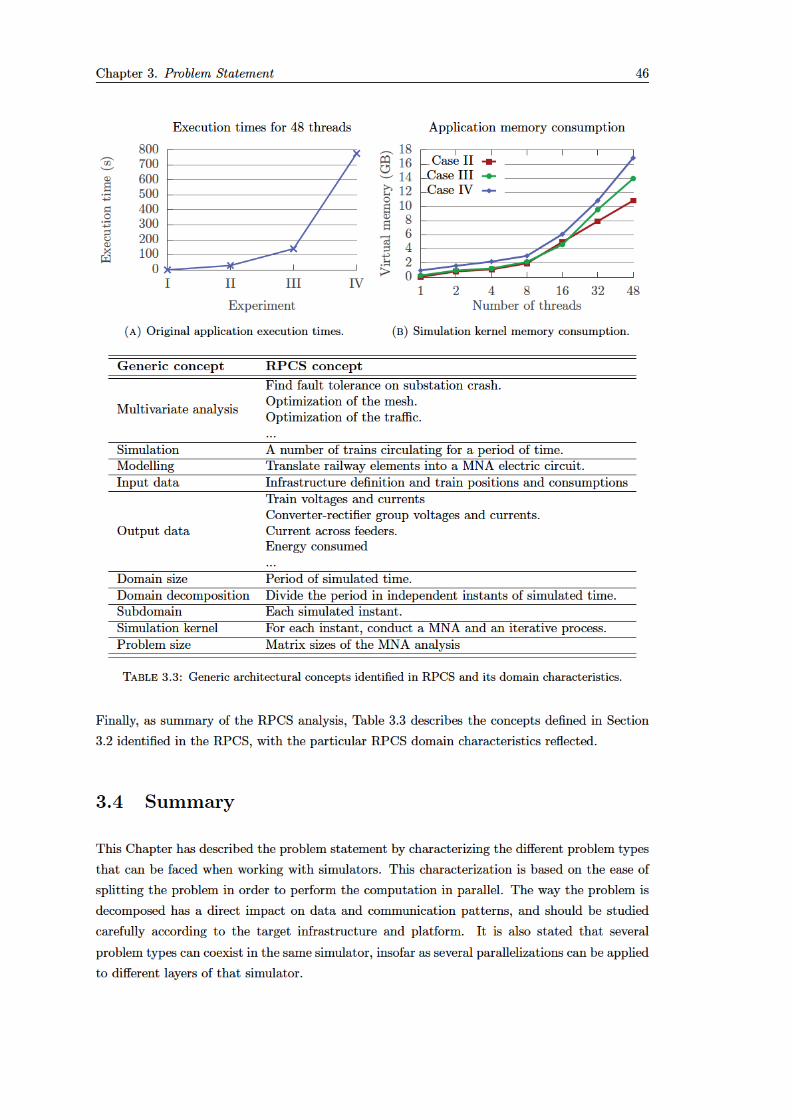

Chapter 3. Problem Statement 47
As contribution, the chapter also has described the RPCS, a railway power consumption simu-
lator developed by UC3M in collaboration with ADIF, the Spanish railway company. With the
aim of serving as case study, this simulator is analysed from the point of view described before,
pointing the different layers where opportunities for applying parallelization lie. In subsequent
chapters, parallelization on such layers will be applied, targeting different infrastructures and
platforms, and analysing the results obtained.


Chapter 4
High Performance Computing
Approaches to Problem
Decomposition
The previous chapter has described the different problem types that must be faced when working
with simulators. This characterization is based on how easy the problem domain can be split,
provided that it has a direct impact on data and communication patterns. The previous chapter
has also shown two kinds of infrastructures (HPC and Cloud), and two kinds of solutions (MPI
and MapReduce) very related to the execution of extensive parallel simulations.
This chapter explores different HPC-based approaches to problem decomposition. Starting from
the generic architecture proposed in the previous chapter (see Figure 3.5), two different ap-
proaches using message-passing techniques are described. The first one tackles the medium
layer of those described in Figure 3.6, applying parallelism through domain decomposition. This
approach will be described in Section 4.1. The second one tackles the lowest layer (see Fig-
ure 3.6 again) applying parallelism to the algebraic operations that usually represent the main
computing workload of the simulation kernels. This approach will be described in Section 4.2.
In order to evaluate the feasibility of both approaches, the RPCS (described in Section 3.3) will be
used as case study, so both will be implemented within the application, and evaluated separately
using MPI, which is the de-facto standard in HPC. Implementation details will be described
in Section 4.3. The evaluations will be conducted under HPC and Cloud infrastructures, in
order to analyze the performance with regard to the underlying infrastructure which is running
the simulation. These results will show the suitability and limitations of the aforementioned
approaches according to the infrastructure used.
49

Chapter 4. HPC Approaches 50
4.1 Domain Decomposition Approaches in HPC
The first HPC approaches to be explored are based on domain decomposition. This approach
starts from the generic simulator architecture described in Section 3.2.1, and the possible paral-
lelization layers and their complexity exposed in sections 3.2.2 and 3.2.3. In domain decomposi-
tion, the whole simulation domain is scattered across the compute nodes, and each compute node
executes the simulation kernel once per received partition. Resulting from the kernel executions,
partial results are obtained on each node. Finally, these partial results are merged in order to
obtain the final simulation result.
The key aspect in this approach is the degree of coupling in the simulation domain. If such
domain can be decomposed easily in partitions, and processing each partition does not require
to swap data with another one, the communications required to conduct the simulation will be
reduced to the minimum. On the contrary, a tightly coupled domain may require exchanges of
data between all partitions, leading to an explosive amount of communications as the number of
nodes is increased.
Besides, this approach implies that the whole simulation kernel is going to be executed sequen-
tially, and each partition will be stored in the memory of the node. CPU intensive simulation
kernels may take too long to be solved, and memory intensive kernels may require more memory
than that available in the compute node. The advantages of this approach lie in the best case: a
pleasingly parallel problem and a not so demanding kernels. In this case this approach is the eas-
iest to implement, and the fastest (in terms of execution times) due to absence of communication
delays.
Two generic algorithms for domain decomposition are described: using a coordinator process
and using collective I/O. We assume familiarization with MPI-like programming model (same
program, multiple processes), and communications (point-to-point and collective operations).
4.1.1 Domain Decomposition Using a Coordinator Process
Algorithm 2 illustrates the code of a simulator implementing domain decomposition, and using a
coordinator process. In this code, a coordinator process (usually rank 0 in MPI applications) is
accountable for the initial and final stages of reading the simulation data and writing the results.
The coordinator process reads from the storage both the global data Iglob (used all through the
simulation) and the domain data Idom (which can be decomposed). The global data is then
broadcasted, and the domain data is scattered to all other processes. Each process receives a
subset Ip which contains one or more partitions Ii so that they are able to execute the simulation
kernel over their own subset of data.
After (or during) the executing of the simulation kernel, exchanges of data between domain
partitions may occur. A pleasingly parallel problem may not require any exchange, but some
simulations may require communication between a constant, reduced set of related processes (like
the ghost region, the boundaries between mesh partitions, or any other kind of neighbourhood),
and some others may require that each process broadcasts its partial results. This has been

Chapter 4. HPC Approaches 51
Algorithm 2 Message-passing approach to domain decomposition using a coordinator process.
Input: {Path-Iglob, Path-Idom}Output: O1:
2: if coordinator then ⊲ Coordinator reads data and splits the simulation domain.3: Iglob ← Read(Path-Iglob)4: Idom ← Read(Path-Idom)5: Broadcastsnd(Iglob)6: Scattersnd(Idom)7: else8: Iglob ← Broadcastrcv()9: Ip ← Scatterrcv()
10: end if11:
12: for all (Ii ∈ Ip) do ⊲ Every process executes the simulation kernel on its own partition.13: Oi ← SimulationKernel(Iglob, Ii)14: SolveCoupling(Oi)15: Op ← Op +Oi
16: end for17:
18: if coordinator then ⊲ Coordinator gathers all output and writes the results.19: O ← Gatherrcv()20: Write(O)21: else22: Gathersnd(Op)23: end if24:
25: function SolveCoupling(Oi) ⊲ Depends on domain coupling, it can be:26: if Pleasingly parallel then do-nothing27: end if ⊲ Communications not required28: if Loosely coupled then send-to-k-processes29: end if ⊲ K exchanges per process30: if Tightly coupled then all-gather31: end if ⊲ All processes exchange data32: end function
represented in the algorithm with the SolveCoupling function. Finally, after the execution of the
kernels, the coordinator process is accountable for gathering the partial results of each process
Op and merging the final output O.
This algorithm is easy to implement, provided it does not require the use of advanced I/O, data
layouts, and parallel file systems. Nevertheless, it does not scale up as the simulated domain
increases in size. This is due to the asymmetry in the role of the coordinator process, which has
to maintain in memory the whole domain data, between reading it from storage and scattering
it to the other processes. Most exascale simulation problems tackle domain sizes that do not
allow one single node to maintain the whole domain in memory. In order to cope with this issue,
collective I/O has to be used.

Chapter 4. HPC Approaches 52
Algorithm 3 Message-passing approach to domain decomposition using collective I/O.
Input: {Path-Iglob, Path-Idom}Output: O1:
2: Iview ←TypeCommit(Layout-Idom)3: Oview ←TypeCommit(Layout-O)4:
5: Iglob ← Read(Path-Iglob)6: Ip ← MPI-IO-Read(Path-Idom, rank, Iview)7:
8: for all (Ii ∈ Ip) do ⊲ Every process executes the simulation kernel on its own partition.9: Oi ← SimulationKernel(Iglob, Ii)
10: SolveCoupling(Oi)11: Op ← Op +Oi
12: end for13:
14: MPI-IO-Write(Op, rank,Oview)15:
16: function SolveCoupling(Oi) ⊲ Depends on domain coupling, it can be:17: if Pleasingly parallel then do-nothing18: end if ⊲ Communications not required19: if Loosely coupled then send-to-k-processes20: end if ⊲ K exchanges per process21: if Tightly coupled then all-gather22: end if ⊲ All processes exchange data23: end function
4.1.2 Domain Decomposition Using Collective I/O
Algorithm 3 illustrates the code of a simulator implementing domain decomposition, and using
collective I/O. In this case, there is no coordinator role, so all processes perform a collective read
operation. The data layout in the storage system should be arranged properly, in order to ease
the data reading and distribution performed by the processes collectively. This is done in MPI
by committing a representative type so that all processes can share a global view of the data.
The MPI-IO-Read shown in the algorithm (as simplification of the available I/O functions that
can be found in the MPI standard), is able to read and scatter the data to all processes all at
once. The same principle can be applied to the MPI-IO-Write function, which is able to make
all processes write the data to the storage neatly. Note that, while MPI-IO is referred as the
most common example of collective I/O, this description can be applied to any other kind of
I/O performed parallel and collectively by all ranks, even if these ranks are using the POSIX
inteface, HDF5, or any other kind of I/O.
This approach is more complicated (in terms of development complexity) than the previous one.
It requires the use of advanced I/O and parallel file systems. Besides, the data layout must be
arranged properly. But due to the characteristics of exascale problems, this fashion is usually
required, because when the domain size goes bigger and bigger, it becomes harder to fit in any
node which could act as coordinator. Finally, note that while this approach avoids the necessity
of maintaining the whole domain in physical memory, several issues remain as in the previous
algorithm: the degree of coupling, the serial execution of the kernel, and the need of fitting that
kernel in the physical memory.

Chapter 4. HPC Approaches 53
4.1.3 Communication and Resource Modelling
In order to give an insight into the workings of both implementations, a basic modelling of the
communication and memory usage pattern is proposed. The aim of this basic model is, provided
a simulation domain, to give a rough estimate of the suitability of both implementations in order
to take a first decision. Table 4.1 summarizes the meaning of the symbols used in this section.
Table 4.1: Symbol table for the proposed communication and memory model
Symbol Meaning
α Network latencyβ Network bandwidthm Message size (generic)Tmsg Time required to perform a generic point-to-point communicationTScat Time required to perform a collective Scatter operationTGath Time required to perform a collective Gather operationTBrd Time required to perform a collective Broadcast operationTAllGath Time required to perform a collective AllGather operationp Number of compute processesd Number of I/O serversIglob The (input) global datamglb The size of Iglob dataIdom The (input) domain datamdom The size of Idom dataIp Fraction of the domain data handled by each processO Output datamO The size of O dataTker Time to execute the simulation kernelTCp Time to exchange data after executing the simulation kernelTAlg2 Time to perform the whole algorithm (w/ coordinator proc.)TAlg3 Time to perform the whole algorithm (w/ collective I/O)MAlg2 Memory per proc. required by the whole algorithm (w/ coordinator proc.)MAlg3 Memory per proc. required by the whole algorithm (w/ collective I/O)
The basis of this model is the algorithms and formulas proposed by Thakur and Gropp in
[TG02], based on the Hockney model [Hoc94]. This work focuses on switched networks, which
represent a very simple kind of cluster. Besides, it is unaware of optimizations based on particular
technologies or platforms, so the model can be taken as the worst-case scenario. Given the wide
variety of infrastructures performing HPC nowadays, the model tries to be as generalist as
possible.
The time taken to send a message between any two nodes is independent of the distance, and
can be modelled using the Equation 4.1:
Tmsg(m) = α+mβ (4.1)
where α is the latency per message, m is the message size, and β is the transfer time per byte.
Once this basic transaction has been defined, collective operations can be modelled on the top
of point-to-point communications, in terms of latency, message size, and bandwidth.

Chapter 4. HPC Approaches 54
The Scatter and Gather operations can be modelled using a minimum spanning tree algorithm
(MST), in which each process receives the data from its parent, retains its own slice, and relays
the rest to its children. Let p the number of processes, the Equation 4.2 shows the time required
to perform either Scatter or Gather operation:
TScat(m) = TGath(m) = ⌈lg p⌉α+(p− 1)
pmβ (4.2)
MST algorithm can be used also to implement the Broadcast operation, making the difference
to the previous operation that each process relays the whole set of data, instead of relaying only
a fragment. The Equation 4.3 reflects the time required to complete the operation:
TBrd(m) = ⌈lg p⌉(α+mβ) (4.3)
The AllGather operation can be implemented using a recursive-doubling algorithm. The Equa-
tion 4.4 reflects the time required to perform this operation:
TAllGath(m) = lg pα+(p− 1)
pmβ (4.4)
After modelling the collective communications, the time required to complete the whole Algo-
rithm 2 can be estimated. Let:
• Iglob be the global data.
• Idom be the domain data.
• Ip be the fraction of the domain data handled by each process (according to Equation 4.5).
Each process is assumed to share the same amount of data.
|Ip| =|Idom|
p(4.5)
• O be the output data.
• Tker be the time required to execute the simulation kernel, which is assumed constant
regardless the input data simulated.
The Equation 4.6 represents the total execution time of the Algorithm 2 without considering the
times related to the storage devices:
TAlg2 = TBrd(Iglob) + TScat(Idom) + (|Ip| · Tker) + ((|Ip| − 1) · TCp(O)) + TGath(O) (4.6)
TCp represents the data exchange after executing the kernel, depending on each domain’s degree
of coupling. Equation 4.7 represents this time as a no-op in a pleasingly parallel problem, a

Chapter 4. HPC Approaches 55
constant, small number of communications between nodes (e.g. neighbourhood communication)
for loosely coupled problems, and an AllGather operation in tightly coupled problems where all
nodes have to broadcast their results.
TCp(m) =
∅ for PP
K · Tms(m) : K ≪ p for LC
TAllGath(m) for TC
(4.7)
Note that this exchange is performed (|Ip|−1) times. Due to the fact that the algorithm executes
a Gather operation as final stage, it is redundant to perform the final data collection twice.
Substituting in Equation 4.6 all terms related to collective communications, the total time can
be expressed as a function of the data sizes, the number of processes, and the network latency
and bandwidth, obtaining Equation 4.8. Let:
• mglb be the size of Iglob data.
• mdom be the size of Idom data.
• mO be the size of O data.
TAlg2 = ⌈lg p⌉(α+mglbβ)
+ ⌈lg p⌉α+(p− 1)
pmdomβ
+|Idom|
pTker
+ (|Idom|
p− 1) · (lg pα+
(p− 1)
pmOβ)
+ ⌈lg p⌉α+(p− 1)
pmOβ
(4.8)
Finally, grouping terms α, mglb, mdom, and mO, Equation 4.9 is obtained:
TAlg2 = (3⌈lg p⌉+|Idom| · lg p
p− lg p)α
+ ⌈lg p⌉mglbβ
+(p− 1)
pmdomβ
+|Idom|
pTker
+ (((|Idom|
p− 1) ·
(p− 1)
p) +
(p− 1)
p)mOβ
(4.9)
Analysing the limits of TAlg2 as p approaches to 1 (pure sequential) and to |Idom| (the maximum
degree of parallelism), we obtain:

Chapter 4. HPC Approaches 56
limp→1
TAlg2 = |Idom| · Tker (4.10)
limp→|Idom|
TAlg2 = 3⌈lg p⌉α+ (⌈lg p⌉mglb +(p− 1)
pmdom +
(p− 1)
pmO)β + Tker (4.11)
This allows to establish when it is worthwhile decomposing the problem across a number of
processes, provided the characteristics of the problem (mglb, mdom, etc..) and the network (α,
β) are known.
The maximum memory usage of the algorithm in a single process can be expressed as the
maximum between the domain data (loaded in memory by the coordinator prior to performing
the Scatter operation) and the memory usage required by the kernel at any node (i.e. the size
of the problem):
MAlg2 = Iglob +max(Idom, Ip + SimulationKernel +Op) (4.12)
The total execution time of the Algorithm 3 can also be expressed in the same terms, modelling its
communications and the execution time of the simulation kernel. Nevertheless, in this algorithm
the I/O phases are performed collectively by all processes, and therefore is more difficult to
predict the behaviour of the application in such phases. The Equation 4.13 represents the total
execution time of the algorithm using IOread and IOwrite as the times required to execute the
I/O read and write phases respectively:
TAlg3 = TBrd(Iglob) + IOread + (|Ip| · Tker) + ((|Ip| − 1) · TCp(O)) + IOwrite (4.13)
Collective I/O involves different participants that may influence the global behaviour of the
system: the parallel file system, the number of I/O servers, the I/O network, and the storage
devices. In order to keep the strategy of providing a simple approach, this model focuses on the
number of I/O servers, assuming a switched network similar to that assumed between compute
nodes. Other elements are not considered, and the algorithms implemented within MPI-IO are
considered to be the same as those previously described in common collective communications
(e.g. MST when an IO server is gathering the data). Let d the number of I/O servers, Equation
4.14 represents the times required to perform the collective I/O, without considering the storage
devices:
IOread =⌈lg p⌉
⌈lg d⌉α+
(p)
dmdomβ
IOwrite =⌈lg p⌉
⌈lg d⌉α+
(p)
dmOβ
(4.14)
With this approach, if there is only one I/O server (the worst case), IOread and IOwrite opera-
tions become Scatter and Gather respectively (see equations 4.6 to 4.9), sending the data from

Chapter 4. HPC Approaches 57
the server to the compute nodes, or receiving the data from the compute nodes to the server.
The best case is achieved when there is a one to one ratio between I/O servers and compute
nodes. In that case, IOread and IOwrite operations become single point to point communication:
each compute node exchanging data with its I/O pair.
TAlg3 = ⌈lg p⌉(α+mglbβ)
+⌈lg p⌉
⌈lg d⌉α+
(p)
dmdomβ
+|Idom|
pTker
+ (|Idom|
p− 1) · (lg pα+
(p− 1)
pmOβ)
+⌈lg p⌉
⌈lg d⌉α+
p
dmOβ
(4.15)
Finally, grouping terms α, mglb, mdom, and mO, Equation 4.16 is obtained:
TAlg3 = (⌈lg p⌉+ 2⌈lg p⌉
⌈lg d⌉+ (|Idom|
p− 1) lg p)α
+ ⌈lg p⌉mglbβ
+(p)
dmdomβ
+|Idom|
pTker
+ (((|Idom|
p− 1) ·
(p− 1)
p) +
p
d)mOβ
(4.16)
In this algorithm, the maximum memory usage per single process can be expressed as the size
of its corresponding share of domain data, plus the global data and the memory consumption
brought by the simulation kernel (i.e. the size of the problem):
MAlg3 = Iglob + Ip + SimulationKernel +Op (4.17)
4.2 Matrix Decomposition Approaches in HPC
Once the domain decomposition has been explored, the next approaches to be analysed are the
matrix decompositions. In matrix decomposition, the algebraic operations that represent the
simulation kernel are performed in parallel across all cluster nodes (e.g. multiplication, trans-
position, inversion, etc.) and the fragments of the matrices used by the simulation are scattered
(or read in parallel) across the cluster. Usually a simulation requires several executions of the
simulation kernel, In such cases each one of these executions will be performed in parallel across

Chapter 4. HPC Approaches 58
the whole cluster, but sequentially regarding the simulation life cycle, because each execution
makes use of all available resources.
Far from the previous approach where the degree of coupling was dependant on the particular do-
main, matrix operations are always tightly coupled, requiring a high number of communications
to be performed. This supposes a serious handicap in medium or low speed networks with high
latencies, and that is the main reason for putting a lot of effort in optimizing high-performance
networks, topologies, and those related topics. The main advantage of this approach is that due
to the fact that the whole simulation kernel is decomposed, it is possible to lower the amount of
memory required by the compute nodes to execute the kernel. By sharing each node a piece of
the matrix (or matrices), no matter how big the problem size is, we can just add more and more
nodes to tackle it.
4.2.1 Matrix Decomposition Using Master-Slaves
Algorithm 4 illustrates the code of a simulator implementing matrix decomposition. This code
uses a master-slaves scheme, where a leading process drives the simulation stages (see Master
function), and dispatches the operations, whereas the slave processes (see Slave function) take
the bulk of the simulation sharing the workload associated to the matrix operations. The leading
process may also share its own part of the workload, so as to make all processes use the same
resources.
This scheme is useful when the simulation requires additional logic apart from the simulation
kernel, having to choose, for instance, between different kernels, or different operations within
the same kernel, depending on some data. In order to do so, the coordinator, which is driving the
simulation, and therefore knows what is the forthcoming operation, broadcasts a corresponding
code as well as any additional arguments of such operation (see SimulationKernel function),
making all slaves proceed in coordination. The slaves follow the pattern of a finite-state machine
(FSM), waiting for a code, and then executing the corresponding operation, until the simulation
finishes.
As in the previous algorithms, I/O can be performed through the coordinator process or collec-
tively. Regarding this, the same advantages and shortcomings described in the previous section
remain, being the collective I/O the most suitable code as the domain and/or problem sizes be-
come large. Algorithm 4 illustrates the coordinator process case, but a collective I/O approach
could be implemented easily by adding to the slaves another DistributedMatrixOP operation,
which could read (or write) the matrix data collectively, and remaining the master as the driver
of the simulation.
4.2.2 Communication and Resource Modelling Example: LU Inversion
Whereas in Section 4.1.3 a basic model has been given, in order to estimate roughly the com-
munication burden of the algorithms described in sections 4.1.1 and 4.1.2, it is not possible to
proceed in the same way with the matrix decomposition approach. The fact is that there is a

Chapter 4. HPC Approaches 59
Algorithm 4 Message-passing approach to matrix decomposition using master-slave scheme.
Input: {Path-Iglob, Path-Idom}Output: O1:
2: if coordinator then ⊲ Master process drives the simulation.3: Master(Path-Iglob, Path-Idom)4: else5: Slave()6: end if7:
8: function Master(Path-Iglob, Path-Idom)9: Iglob ← Read(Path-Iglob) ⊲ I/O through coordinator process.
10: Idom ← Read(Path-Idom)11: for all (Ii ∈ Idom) do12: Oi ← SimulationKernel(Iglob, Ii)13: O ← O +Oi
14: end for15: Write(O)16: end function17:
18: function SimulationKernel(Iglob, Ii)19: ... ⊲ Master distributes matrix op. codes across the slaves.20: Broadcastsnd(OP1)21: DistributedMatrixOP1(Matrix)22: ...23: Scattersnd(OP2)24: DistributedMatrixOP2(Matrix)25: ...26: Broadcastsnd(OPend)27: end function28:
29: function Slave ⊲ Slaves execute matrix operations.30: while !end do31: OP ← Broadcastrcv()32: if OP = OP1 then DistributedMatrixOP1()33: end if34: if OP = OP2 then DistributedMatrixOP2()35: end if36: ...37: if OP = OPend then end← true38: end if39: end while40: end function
huge amount of different simulation kernels and algebraic operations, each one of them perform-
ing a different communication pattern. A very brief list of some of these kernels can be found in
[Jam12].
Nevertheless, it is possible to develop the same model with one example of matrix operation, and
then extend the conclusions to those operations that are more complex than the illustrated one.
The operation to be analysed is matrix inversion based on the LU factorization. Let a system
of linear equations in matrix form:

Chapter 4. HPC Approaches 60
Ax = b (4.18)
The square matrix A ∈ Rn×n is invertible if there exists a matrix A−1 ∈ R
n×n such that:
A−1A = AA−1 = I (4.19)
If we have computed the LU decomposition: A = LU then we can replace A in the system. This
leads to two linear systems:
Ly = b (4.20a)
Ux = y (4.20b)
Solving both systems brings the solution b easily. Note that we are not analysing the LU
factorization, but the matrix inversion once the matrix has been factorized. The Listing 4.1
shows a simplified code of the LU inversion that does not perform partial pivoting, using MPI:

Chapter 4. HPC Approaches 61
1 // Solve L*Y = I
for (int k = 0; k < cols; k++){
MPI_Barrier( MPI_COMM_WORLD );
// Send k row to all
6 if(k >= startingrow[slaverank] && k < finalrow[slaverank ]){
for(int p = slaverank + 1; p < slavesize; p++){
MPI_Send( &ret[k * cols], cols , MPI_DOUBLE , p, 1980, MPI_COMM_WORLD);
}
}
11 else if(k < startingrow[slaverank ]){
// Receive
MPI_Recv( &ret[k * cols], cols , MPI_DOUBLE , MPI_ANY_SOURCE , 1980, MPI_COMM_WORLD ,
MPI_STATUS_IGNORE);
}
16 // Update lower rows using k
for (int i = max(k + 1, startingrow[slaverank ]); i < finalrow[slaverank ]; i++){
for (int j = 0; j < cols; j++){
ret[i * cols + j] = ret[i * cols + j] - (ret[k * cols + j] * lu[i * cols + k]);
}
21 }
}
// Solve U*X = Y;
for (int k = cols - 1; k >= 0; k--){
26 MPI_Barrier( MPI_COMM_WORLD );
if(k >= startingrow[slaverank] && k < finalrow[slaverank ]){
// Update k row using diagonal
for (int j = 0; j < cols; j++){
ret[k * cols + j] /= lu[k * cols + k];
31 }
for(int p = slaverank - 1; p >= 0; p--){
// Send k row to all
MPI_Send( &ret[k * cols], cols , MPI_DOUBLE , p, 1975, MPI_COMM_WORLD);
36 }
}
else if(k >= finalrow[slaverank ]){
// Receive
MPI_Recv( &ret[k * cols], cols , MPI_DOUBLE , MPI_ANY_SOURCE , 1975, MPI_COMM_WORLD ,
MPI_STATUS_IGNORE);
41 }
// Update upper rows using k
for (int i = startingrow[slaverank ]; i < min(k, finalrow[slaverank ]); i++){
for (int j = 0; j < cols; j++){
46 ret[i * cols + j] = ret[i * cols + j] - (ret[k * cols + j] * lu[i * cols + k]);
}
}
}
Listing 4.1: MPI implementation of a matrix inversion using LU decomposition w/o partial
pivoting
The main matrix is scattered (or read collectively) across the processes by rows. Then, there are
two main loops in the code that iterate across the rows of the matrix. Up to down in the first
one, and down to up in the second. For each iteration, the process accountable for the current
(k) row broadcasts it to the processes holding the inferior (in the first loop) or superior (in the
second loop) rows. Then, all processes update their part of the matrix using the received row.
The following enumeration summarizes the estimation of the communications:
Chapter 4. HPC Approaches 62
1. For simplicity, it is assumed that the matrix (of size n × n) has been evenly distributed
across a number of p processes. Therefore each process shares nprows, each one of size n.
2. Each process pi ∈ p has to send its nprows to the lower (or upper) ranks. Let ri ∈ [0, p−1]
the rank of the process pi, and let ti the times the process pi sends a message:
∀pi ∈ p, ti =n
p(p− ri + 1) (4.21)
3. Therefore, the total number of messages for each loop ttot will be:
ttot =∑
i
n
p(p− ri + 1) =
n
p
∑
i
(p− ri + 1) (4.22)
4. Considering both loops, Equation 4.1 which defines the time required to send a message,
and the fact that all messages are equal in size m = n, the total communication time
required to perform the LU inversion is:
TLU−1 = 2 · ttot · Tmsg =2n
p
∑
i
(p− ri + 1)(α+ nβ) (4.23)
5. Finally, applying the divergent series:
n∑
k=1
k =n(n+ 1)
2(4.24)
6. The TLU−1 can be approached as follows:
TLU−1 = n(p+ 1)(α+ nβ) (4.25)
Therefore the communication time TLU−1 is quadratic to the matrix dimension d and linear
to the number of processes p, but due to the fact that, as the matrices go bigger, more nodes
have to be used (in order to decrease the execution times), both magnitudes can be considered
directly proportional: p ∝ n. So we can consider that the communication time TLU−1 is cubic to
matrix dimension d or cubic to the number of processes p if a proportionality constant n = kp
is established.
4.3 Application to RPCS
To illustrate and evaluate how the HPC approaches shown in the previous sections perform on
different infrastructures, both of them were implemented within the RPCS simulator described
in Chapter 3. Parallelism to the RPCS can be applied at different layers, either performing
a domain decomposition, or applying parallelism to the simulation kernel that performs the
MNA. So Section 4.3.1 will describe the domain decomposition approach implemented within
the RPCS, and Section 4.3.2 will describe the matrix decomposition implementation within the
RPCS. Both implementations do not overlap, and are maintained as separate subversions of the
application.

Chapter 4. HPC Approaches 63
4.3.1 Domain Decomposition in RPCS
The RPCS simulates the electric behaviour of a railway infrastructure during a period of time
in which the trains are circulating across the lines. This period is defined by the user, and
may be from several minutes in the smallest simulations, to several weeks or even one month if
the user wants to analyse the behaviour of the system in a long-term plan. The simulation is
conducted analysing the behaviour of the electric circuit in each one of the seconds that compose
this period. The positions and consumptions of the trains are know for each one of such seconds,
and taken as input data of the simulations, so there are no dependences between the simulations
of different seconds even if they belong to the same period.
As it is described in Table 3.3, the simulated time period can be considered as the simulation
domain, and the MNA performed in each one of the simulated seconds is the simulation kernel.
Therefore, the whole simulation period will be decomposed in several subintervals with lower
magnitude, and each one of this subintervals will be simulated by a different worker. For instance,
if the whole simulation period is from the 06:00:00 hours to the 22:00:00 hours and the number
of workers is 4:
• The 1st worker will handle from 06:00:00 hours to 09:59:59 hours.
• The 2nd worker will handle from 10:00:00 hours to 13:59:59 hours.
• The 3rd worker will handle from 14:00:00 hours to 17:59:59 hours.
• The 4th worker will handle from 18:00:00 hours to 22:00:00 hours.
In order to avoid the asymmetric role of a coordinator process, the algorithm to be implemented
will be based on collective I/O (see Algorithm 3). Implementation details are listed below:
• The infrastructure file, which defines the invariant elements of the circuit common to all
simulated instants (tracks, catenaries, power stations, etc.), is considered as the global
data.
• The train data files, which contain the positions and consumptions of each train along
the simulated period, are considered as the domain data. The domain distribution will be
based on MPI ranks: the process with the first rank will handle the first subinterval, and
son on.
• All I/O will be handled by POSIX system calls, and MPI-IO will not be used. This is
because most of the input data is based on text, so the structured layout usually used in
MPI-IO does not fit properly when reading lines of variable length. Besides, test-based
input and output is a requirement of the original application, in order to ease the post-
processing and analysis of the results. On reading data, this does not suppose a problem,
because common file systems can handle parallel readings easily. Besides, parallel file
systems implement also the POSIX interface in order to give support to basic operations.
On the contrary, writing data in parallel to the same file supposes a risk of losing coherence,
due to interleaved or disordered writings. In order to cope with this issue, each worker will
write data to its own file, and all files created by workers will be merged in a final stage.

Chapter 4. HPC Approaches 64
• Apart from the final merger of the files created by workers, there are no dependences
between domain partitions, so no data must be exchanged between workers every time the
simulation kernel is executed.
4.3.2 Matrix Decomposition in RPCS
In order to apply matrix decomposition to the RPCS, it is necessary to analyze first what are
matrix operations that are performed within the kernel. Two different sources are used to get this
information: the application technical report which contains the description of the mathematical
and electrical principles implemented, and an application profile, obtained using gconf utility,
which identifies the top execution time functions. The list is displayed in Table 4.2.
Table 4.2: Execution profile of RPCS from gprof utility: top execution time functions list
Each sample counts as 0.01 seconds
%time
cumulativeseconds
selfseconds
callsselfs/call
totals/call
name
66.84 1086.57 1086.57 16752 0.00 0.00 ArrayOperator::Inv(...)22.85 1458.02 371.45 16752 0.00 0.00 LUMatrix::Factorize()9.70 1615.74 157.72 47658 0.00 0.00 ArrayOperator::MultiplyMatrix(...)0.28 1620.36 4.62 25521 0.00 0.00 ArrayOperator::MultiplyMatrix(...)...
These analyses identify four major matrix operations which are conducted during the execution
of the kernel. They are listed below, ordered proportionally according to their relative execution
times respect to the whole kernel:
• Matrix inversion, provided that the matrix has been factorized before (performed by the
ArrayOperator::Inv() function).
• LU factorization with partial pivoting (PA-LU) (performed by the LUMatrix::Factorize()
function).
• Matrix multiplication (performed by the ArrayOperator::MultiplyMatrix() function).
Matrix factorization and inversion take the most of the simulation kernel’s execution time, so
applying parallelism to that functions is the most urgent task. LU decomposition with partial
pivoting complicates the implementation and significantly affects potential performance [Hea11].
Nevertheless, partial pivoting is required to ensure existence and numerical stability of the fac-
torization. In order to optimize as much as possible these two operations, a specialized algebraic
library such as ScaLAPACK (as well as its dependences LAPACK and BLAS) is integrated with
the RPCS. ScaLAPACK [BCC+97] implements a a block cyclic data distribution for dense ma-
trices and block-partitioned algorithms that minimize the frequency of data movement between
different levels of the memory hierarchy (including off-processor memory of other processors).
The following routines will be invoked from the RPCS:


Chapter 4. HPC Approaches 66
4.4 Evaluation
In order to assess the behaviour of the two approaches described in this chapter, an evaluation
is conducted using the two versions of the RPCS described in the previous section: with domain
decomposition and with matrix decomposition. This evaluation is conducted under two kinds
of infrastructures, an HPC cluster and a Cloud of virtual instances deployed in Amazon EC2.
The aim is to identify the trends of both approaches as the low level optimizations characteristic
of HPC systems disappear in favour of the Cloud characteristics and limitations. Table 4.3
summarizes the characteristics of the nodes that compose these two kinds of infrastructures.
Table 4.3: Node features for the HPC cluster and the Cloud used in the evaluation
HPC cluster node Amazon EC2 Cloud node
ProcessorIntelr Xeonr
E5405 2.00GHzIntelr Xeonr
E5-2680 (v2) 2.80GHzPhysical mem. 8.0 GB DDR2 7.5 GB DDR3
Network InfiniBand DDRUnspecified
(moderate performance)1
Topology Flat UnknownCompiler ICC 15.0.1 GCC 4.8.1Libraries (DD) Netlib LAPACK Netlib LAPACK
Libraries (MD) Intelr MKL 11.3Netlib ScaLAPACK
OpenBLASFile System GlusterFS NFSv4Op. mode (DD) Process per core (MPI) Process per core (MPI)
Op. mode (MD)Process per node(MPI + OpenMP)
Process per node(MPI + pthreads)
The HPC cluster features the common characteristics of HPC infrastructures. It deploys a
high-bandwidth low-latency interconnect network, in a well-known static topology. RPCS im-
plementations have been compiled using the Intelr ICC compiler, in order to take advantage of
that optimizations available for the particular processor model and architecture installed in the
cluster nodes. Besides, the Intelr Math Kernel Library (MKL) has been used as implementation
of ScaLAPACK, LAPACK, and BLAS routines.
On the contrary, the Cloud allocated in Amazon EC2 features the characteristics of Cloud en-
vironments, with little or no optimizations based on the particular hardware architecture. The
c3.xlarge has been selected as the instance type most similar to the cluster nodes in terms of
processing power and physical memory. While Amazon describes in the documentation that the
processor model supporting the c3.xlarge instance type is an E5-2680 Ivy Bridge, it has been
decided to not take advantage of this information when compiling the application, provided that
other instance types, and therefore other processor models (or even other processor brands), may
be selected according to the particular requirements of the user at forthcoming executions. Fol-
lowing the same philosophy, the compiler used has been GCC, and the ScaLAPACK, LAPACK,
and BLAS implementations used have not been those provided by Intelr. Instead, the Netlib
implementation of ScaLAPACK and LAPACK, and the GotoBLAS2[GVDG08] implementation
of BLAS have been used, because they target a wider catalog of architectures than the MKL
1Measurements through iperf commands suggest a 1Gbps network

Chapter 4. HPC Approaches 67
Table 4.4: Test cases definition for the HPC-based approaches.
Experiment Simulated Input Version
time size (MB) tested
I ≈ 1 hour 1.7 Matrix dec. only
II ≈ 1 day 170 Domain dec. and Matrix dec.
III ≈ 1 week 1228.8 Domain dec. and Matrix dec.
IV ≈ 1 month 5324.8 Domain dec. only
[Edd10]. Finally, Amazon EC2 does not provide information about the network that supports
the virtual machines, apart from an ambiguous ”Moderate” referred to the quality of the network
connection. Nevertheless, measurements through iperf tool between allocated instances suggest
that the network bandwidth is approximately 1Gbps.
The test cases simulated during this evaluation are summarised in Table 4.4. These tests are the
same that were used in Chapter 3 to conduct a resource analysis of the original RPCS application
(also the same that will be used in Chapter 5). Each one of these experiments (numbered as
I, II, III, and IV) suppose an increment in both domain size (period of time to be simulated)
and problem size (size of the electric circuit) with regard to the previous one. They will be
tested using both approaches implemented (domain decomposition and matrix decomposition),
in both infrastructures (the HPC cluster and the Cloud), and with a variable number of nodes
in infrastructure (for 2, 4, 6, 8, and 10 nodes).
Due to the large amount of experiments that are going to be simulated, the simulation step has
been increased to from 1 to 120 seconds. Therefore, only one of each 120 instants of the simulation
interval will be simulated. Besides, due to the fact that the domain size of the Experiment I is
very small, it will not be tested using the domain decomposition approach. Similarly, due to
the fact that the domain size of the Experiment IV is very large, it will not be tested using the
matrix decomposition approach.
4.4.1 Domain Decomposition Evaluation
The domain decomposition approach was the first to be evaluated. Figure 4.2 shows the RPCS
execution times, when simulating the Experiments II, III, and IV, as the number of nodes in
both the HPC cluster and the Amazon Cloud is increased. The figure shows times corresponding
to the initial input phase in which all the global and domain data is loaded (a, c, and e), and
the times corresponding to the actual simulation (b, d, and f). The following conclusions can be
extracted from the results shown:
• Regarding the compute phase, the application expresses a good degree of scalability up
to 10 nodes (40 MPI processes) regardless of the infrastructure used. Compute times
descend linearly as more nodes are added for all infrastructure size tested. The absence of
communication inside the simulation kernel, as well as the fact that the whole simulation


Chapter 4. HPC Approaches 69
• Regarding the input phase, the GlusterFS in the HPC cluster shows overall better results
than the NFSv4 in the Amazon Cloud for the Experiments II and III. Actually, the input
phase times in the cluster remains constant for these experiments, indicating that the
volume of the input data is not big enough to overcome the bandwidth of the file system.
The same is not happening in the Cloud, where the input phase times are increased as
more nodes read the data from the NFS server.
4.4.2 Matrix Decomposition Evaluation
After evaluating the domain decomposition approach, we proceeded to evaluate the matrix de-
composition implementation. Figure 4.3 shows the RPCS execution times, when simulating the
Experiments I, II, and III, as the number of nodes is increased in both the HPC cluster and the
Amazon Cloud. The figure shows times corresponding only to the actual simulation, discarding
the initial and final phases. The following conclusions can be extracted from the results:
• For all experiments tested, and for both architectures, the application’s execution times are
increased as more nodes are added to the infrastructure. This demonstrates how sensible
is the application to the communication overhead, as expected using matrix decomposition
(see Equation 4.25), but also denotes that the size of the operated matrices is not big
enough to make the parallel execution worthwhile. The number of operations performed
in parallel does not compensate the latencies suffered when communicating through the
network, even if using a high-performance low-latency network. Nevertheless, the main
advantage of this approach is the distribution of the memory workload among all the
cluster, in that cases where the simulation kernel does not fit in the memory of a single
node.
• As expected, the HPC cluster achieves better overall performance, since outperforms the
Amazon Cloud in every direct comparison. Besides, the HPC cluster shows better scala-
bility, since the growth in the execution times is far less steep than in the Amazon Cloud.
Even through the HPC cluster is somewhat outdated compared to the underlying Amazon
infrastructure (see Table 4.3 for comparison), the superior quality of the network has a
great impact on these tightly coupled algorithms.
4.5 Summary
In this chapter we have explored HPC approaches to problem decomposition, starting from the
generic architecture proposed in Chapter 3. Two different approaches using message-passing
techniques are described: domain decomposition and matrix decomposition. Domain decompo-
sition relies on splitting the simulation domain in multiple subdomains and executing in parallel
the simulation kernel on each subdomain, while matrix decomposition applies parallelization in
the matrix operations that compose the simulation kernel.
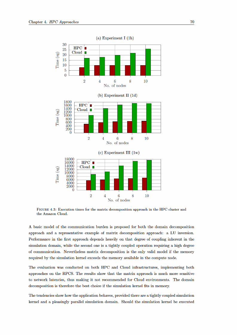

Chapter 4. HPC Approaches 71
sequentially, the most relevant feature in the infrastructure is the CPU (even if platform specific
optimizations are not available). On the contrary, should the simulation kernel be executed
in parallel, the network has the deepest impact on the execution times. In terms of workload
sharing, the bigger the simulation domain is, the easier is to distribute the workload evenly among
the cluster through domain decomposition. On the contrary, if the computing requirements of
the simulation kernel are high enough, it can be meaningful to perform the matrix computations
in parallel, even through these operations are tightly coupled.
Finally, there are several shortages common to both approaches. First of all, MPI (at least at
the standard level) does not bring any fault tolerance to the applications. Secondly, MPI neither
provides elasticity mechanisms to adapt the application to changes in the infrastructure, so Cloud
elasticity can not be exploited. All things considered, we turn towards domain decomposition
using data centric approaches based on the MapReduce framework, which can bring these desired
features.


Chapter 5
A Methodology to Migrate
Simulations to Cloud Computing
In the previous chapter, the traditional approaches to parallelizing modern simulators have been
explored. Message-passing techniques were used over cluster resources, applying the paralleliza-
tion at different levels of the simulator proposed as case study. Once traditional approaches have
been explored, this thesis turn towards Cloud technologies.
In this chapter, a generic methodology to transform modern simulators into a cloud-suitable data-
centric scheme via the MapReduce framework is proposed. The aim of this thesis proposal is to
exploit Cloud advantages in modern simulators, such as virtual unlimited scalability of hardware
resources, platform independence, and flexibility according to instantaneous user needs (through
adapting computing resources). The focus is on Map-Reduce because this platform, as well as
the data-centric scheme that proposes, is suitable for Cloud Computing, but also can perform
efficiently on clusters and supercomputers.
5.1 Methodology Description
The MapReduce paradigm consists of two user-defined operations: map and reduce. The former
takes the input and produces a set of intermediate (key, value) pairs that will be organized by
key by the framework, so that every reducer gets a set of values that correspond to a particular
key [DG08].
As a data-centric paradigm, in which large amounts of information can be potentially processed,
these operations run independently and only rely upon the input data they are fed with. Thus,
several instances can run simultaneously with no further interdependence. Moreover, data can
be spread across as many nodes as needed to deal with scalability issues.
Simulations, however, are usually resource-intensive in terms of CPU or memory usage, so their
scalability is limited to hardware restrictions, even in large clusters. The goal is to exploit
73

Chapter 5. Cloud Methodology 74
the data-centric paradigm to achieve a virtually infinite scalability. This would permit the
execution of large numeric simulations independently of the underlying hardware resources, with
minimal effects to the original simulation code. From this point of view, numeric simulations
would become more sustainable, allowing us to spread simulation scenarios of different sizes in a
more flexible way, using heterogeneous hardware, and taking advantage of shared inter-domain
infrastructures.
To achieve this, this proposal takes advantage of MapReduce’s lack of task interdependence and
data-centric design. This will allow to disseminate the simulation’s original input to distribute
its load among the available nodes, which will yield the scalability we aim for. The steps involved
in the proposed methodology are described in the following sections.
5.1.1 Methodology Terms and Definitions
The first step is defining several key concepts in which the methodology is going to be based on.
Let S be the whole simulation process, which receives an input data set I, applies a function
fsim(x) over that input, and produces an output data set O.
S ≡ fsim(I) = O (5.1)
The output data O can be organized in multiple files, each one containing different results from
the simulation:
O ≡ {O0, O1, ..., Om} (5.2)
The input data I can be classified in two different types:
• Global data Iglob. This kind of data does not vary with regard to the problem domain,
maintaining all values constant all along the simulation. In this category may fall those
parameters which are used to configure the simulation globally, read once, applied many
times.
• Domain data Ix. This kind of problems represents the particular scenario to be simulated.
It can be decomposed in different subsets with regard to the problem domain, represent-
ing different dimensions of the problem: a collection of registers that can be processed
independently, different sub-areas of a continuous domain, or different instants in a time
independent simulation.
Therefore, I = {Iglob, I0, I1, I2, ..., Ik} where there are k subdivisions of the domain input data.
Assuming that the problem can be solved in a parallel manner, the function fsim(x) is formulated
as a reduction, fred, of multiple sub-pieces of the input data, after being processed by some
function fker(x), which implements the main logic of the simulation, but applied only to a part
of the problem domain.


Chapter 5. Cloud Methodology 76
Hence, the original simulation domain must be analysed in order to find an independent variable
–Tx in Figure 5.1– that can act as index for the partitioned input data and the following pro-
cedures. This independent variable would be present either in the input data or the simulation
parameters and it could represent, for example, independent time-domain steps, spatial divisions
or a range of simulation parameters.
At the moment, the analysis and selection of such variable is done by direct examination of the
original application. As this process is critical, and it is intimately related with the application’s
structure, procedures and input, it should be performed by an expert in the simulator to be
cloudified. Future work could simplify this stage by mean of automatic analysis and variable
proposal, yet an expert would still be needed to assess the correctness of the suggestion.
5.1.3 Cloudification Process Design
Once verified that the application is suitable for the process, it can be transformed by matching
the input data and independent variables with the elements in Figure 5.1. This results in the
two MapReduce jobs described below:
• Adaptation stage: reads the input files in the map phase and indexes all the necessary
parameters by Tx for every execution as intermediate output. The original data must be
partitioned so that subsequent simulations can run autonomously with all the necessary
data centralized in a unique (Tx, parameters) entry.
• Simulation stage: runs the simulation kernel for each value of the independent variable
along with the necessary data that was mapped to them in the previous stage, plus the
required simulation parameters that are shared by every partition. Since simulations might
generate several output files, mappers would organize the output by means of file identifier
numbers as keys, so as reducers could be able to gather all the output and provide final
results as the original application.
The two algorithms for the adaptation stage are described in Algorithm 5 and Algorithm 6.
Algorithm 5 describes the map phase. During this phase, the input files of the simulation are
processed line by line, in order to extract and arrange all data according to the independent
variable Tx. The task is performed as follows:
1. The input data of the simulation is stored in an HDFS cluster. Chunks of these data are
spread across all nodes and mappers are dispatched to each node in order to process that
chunks.
2. For each chunk, the contents are processed line by line, arranging all lines according to
key-value pairs.
3. If the line contains global data, a specific terminal indicating global contents is assigned
as key, and the value is assigned to the whole line of data.

Chapter 5. Cloud Methodology 77
Algorithm 5 Adaptation phase mapper
Input: IOutput: KV 1 = {(k0, v0), (k1, v1), ..., (kn, vn)}1:
2: for all (chunk ∈ I.files) do3: Map(chunk)4: end for5:
6: function Map(chunk)7: for all (line ∈ chunk) do ⊲ Process input files line by line8: if IsGlobal(line) then ⊲ If line contains global data9: key ← GLOB
10: value← line11: else ⊲ If line contains domain data12: Tx ← FindTx(line) ⊲ Find Tx within the line13: key ← Tx
14: value← line15: end if16: emit(key, value) ⊲ Adds pair to KV1, Tx value as key, the line as value17: end for18: end function
4. If the line contains domain-specific data, the mapper looks for the value of the independent
variable Tx. Once found, this value acts as key, and the value is again the whole line of
data.
5. All key-value pairs are emitted to the reduce phase.
During the reduce phase (described in Algorithm 6) the reducers can group all lines associated
to each value of Tx, thus arranging the input data in an {Iglob, I0, I1, I2, ..., Ik} layout, where
Iglob contains the global data which does not vary with regard to the problem domain, and Ii
contains all data belonging to the ith subdomain partition. The task is performed as follows:
Algorithm 6 Adaptation phase reducer
Input: KV 1 = {(k0, v0), (k1, v1), ..., (kn, vn)}Output: Iglob, I0, I1, I2, I3, ...Ik1:
2: for all ((ki, vi) ∈ KV 1) do3: Reduce((ki, vi))4: end for5:
6: function Reduce((key, value))7: Ii ← DataSetOf(key) ⊲ Find sub-domain partition associated to Tx
8: Ii ← Ii + value ⊲ Group all data associated to Tx in the same set9: end function
1. Each key-value pair emitted by the previous phase is processed by the reducers of this
phase.
2. For each member of the keys set, a dataset is created in order to group all values corre-
sponding to that key.

Chapter 5. Cloud Methodology 78
3. Values are aggregated as the key-value pairs are being processed. The datasets represent
groups of data associated to simulation subdomains.
4. Once all keys have been processed, the datasets are stored in the HDFS.
Once the adaptation stage ends, the simulation stage takes as input the datasets. The simula-
tion stage is described in Algorithm 7 and Algorithm 8. Algorithm 7 describes the map phase.
Starting from the data layout obtained from the previous stage, the mappers execute the simu-
lation kernel, using as input each one of the subdomain partitions. The map task is performed
as follows:
Algorithm 7 Simulation phase mapper
Input: Iglob, I0, I1, I2, I3, ...IkOutput: KV 2 = {(k0, v0), (k1, v1), ..., (kp, vp)}1:
2: for all Ii ∈ I0, .., Ik do3: Map(Iinv, Ii) ⊲ Execute simulation kernel on sub-domain partition4: end for5:
6: function Map(Iinv, Ix)7: Ox = Ox
0 , Ox1 , ..., O
xm ← SimulationKernel(Iinv, Ix)
8: for all Oxi ∈ Ox do ⊲ For each chunk outputted by the kernel
9: key ← i10: value← Ox
i
11: emit(key, value) ⊲ Adds pair to KV2, file ID as key, chunk contents as value12: end for13: end function
1. First of all, the global dataset is spread across all mappers, because it contains data
associated to the whole simulation, so it is needed in all simulation kernels. In order
to do this, the HDFS cache is used. This cache allows to make a small amount of data
available to all nodes in an efficient way. Global data are usually orders of magnitude
smaller than domain data.
2. Datasets containing all simulation subdomains, obtained from the previous stage, are read
by the nodes in the HDFS cluster.
3. The mappers in the nodes execute the simulation kernel on each subdomain. As result,
the simulation is conducted in (concurrent) steps according to the partitions produced in
the previous stage.
4. Each mapper obtains a collection of chunks, fragments of the output files which contain
only the results associated to the simulated partition. The number of chunks depends on
each particular simulation domain characteristics.
5. Finally, mappers emit each chunk using as key an identifier of the final files of the simulation
(e.g if the simulation kernel produces five files, the keys will be k = {0, 1, 2, 3, 4}).
The reduce task (described in Algorithm 8) is accountable for merging each chunk gathering the
results from all mappers. The task is performed as follows:

Chapter 5. Cloud Methodology 79
Algorithm 8 Simulation phase reducer
Input: KV 2 = {(k0, v0), (k1, v1), ..., (kp, vp)}Output: O = {O0, O1, ...Om}1:
2: for all ((ki, vi) ∈ KV 2) do3: Reduce((ki, vi))4: end for5:
6: function Reduce((key, value))7: Oi ← DataSetOf(key) ⊲ Find output file associated to that ID8: Oi ← Oi + value ⊲ Gathers all chunks which corresponds to each output file9: end function
1. Each key-value pair emitted by the previous phase is processed by the reducers of this
phase.
2. Each key represents a final file of the simulation. Data from all simulation kernels are
aggregated and grouped following the same arrangement used in original simulation.
By this way, the resulting files can be composed as if the simulation domain were never split
across the cluster.
5.1.4 Virtual Cluster Planning
The former stages would most likely require different amounts of CPU and memory resources
depending on the application to be cloudified. In this section, a heuristic to detect the slaves’
instance requirements to maximise resource utilisation is provided. First of all, the concept of an
entry is defined. An entry is a piece of data processed by the mappers on any of the methodology
stages. There will be different entries for the adaptation and simulation phases:
• For the adaptation phase, an entry is one of the registers by which the input files are
arranged. Mappers in adaptation phase process these registers indexing them according to
the independent variable Tx.
• For the simulation phase, an entry is one of the Ii = (Tx, parameters) pair. This is the
autonomous piece of data which is going to be simulated by the mappers of the simulation
phase.
Next, the following assumptions are considered:
• All the slaves must be equal in terms of memory and number of cores.
• The execution time required to process an entry, te ∈ R+, is previously known by the user,
and homogeneous for all the entries. For the adaptation phase, this is the time required to
parse an index the parameters according to the independent variable. For the simulation
phase, this is the time required to execute the simulation kernel over a single autonomous
piece of the input data.

Chapter 5. Cloud Methodology 80
• The amount of memory required to process an entry, me ∈ R+, is known and homogeneous
for all the entries. For the adaptation phase, this is the memory needed to perform the
grouping of input parameters according to the independent variable. For the simulation
phase, this is the memory needed to allocate and simulate one single simulation kernel and
merge the results.
• The number of entries, ne ∈ N, is known.
Of course, te and me may vary, depending on the problem domain. In that case the expert should
either estimate an accurate value, or consider inserting probabilistic distributions in formulae.
In the first approach, let assume te and me constant along all entries, in order to simplify
the heuristic. Given these parameters and assumptions, the objective is to minimise the total
execution time of the cloudified application, T ∈ R+. The minimisation problem is defined as
follows:
minnI ,cI
T =tene
nIcI+ α (5.4)
Where cI ∈ N represents the number of cores per instance, nI ∈ N is the number of instances in
the targeted cluster, and α ∈ R+ is a parameter that represents the compute overhead factor of
the underlying platform (spawning the tasks, etc.), which is considered constant.
The following constraint is applied:
mecI + β ≤ mI (5.5)
Where mI ∈ R+ represents the amount of memory per instance and β represents the memory
overhead added by the platform on each instance. Equation 5.5 indicates that the aggregated
memory required by the entries that can be concurrently processed by each node must not exceed
the total memory of it.
Once nI , cI and mI are found, one can select the instances that have greater or equal resources
for both metrics, simultaneously.
This minimisation problem can be modified by letting T be a fixed value, in order to find suitable
instances to meet a specific deadline. This deadline-oriented planning can be very beneficial to
minimise costs in pay-as-you-go infrastructures, as deadlines can be multiples of the time slices
covered by successive charges. For instance, Amazon charges the user for slices of one hour (even
if the user only allocates VMs for 15 minutes). Therefore, this heuristic can be used for:
a) Providing a VM configuration and calculate the expected execution time using that con-
figuration.
b) Choosing the best VM configuration in order to meet a given deadline.

Chapter 5. Cloud Methodology 81
Table 5.1: Examples of virtual cluster planning using different instance types, α = 30s andβ = 1GB.
Objective Problem domain Instance type Ex. time
ne me te cI mI nI T
Calculate T 105 1GB 1s 8 17GB 30 447sSize cluster 105 1GB 1s 2 8GB 15 3600sCalculate T 105 1GB 1s 1 4GB 15 6697s
Examples of the former formulation are shown on Table 5.1, using different instance types. Let
E be the set of ne = 105 entries the user wants to process, each one requiring me = 1GB of
memory and te = 1s for its execution. The first and third rows illustrate contain examples of
calculations of the execution time T provided that the user wants to use 30 instances of 8 cores
and 17GB each (first row), or 15 instances of 1 core and 4GB each (third row). The second
row illustrates the opposite procedure. Assuming the user wants to process E within one hour,
using instances with cI = 2 and mI = 17GB, the execution time, T , becomes a deadline of
3600s. Solving the resulting equation, the number of instances necessary to process all entries
within one hour is 15. Let assume in all examples α = 30s and β = 1GB. Note that memory
optimised machines are meant to favour the memory-bound tasks with a high ratio memory-to-
CPU, whereas compute-bound tasks would benefit from compute optimised instances, as a large
number of cores would allow the execution of more mappers simultaneously.
5.2 Application to RPCS
To illustrate how this methodology works on a real-world use case, we applied it to the RPCS
simulator. This applications is widely described in Chapter 3, as well as the different ways of
applying parallelization at its different layers. Also, as has been explained, the application is
memory-bound, so it is a perfect test case for the methodology. There are multiple advantages
that Cloud Computing could bring to the application. In Section 3.3.4, the analysis of resource
usage performed to the application shows how the workload is strongly dependant on the particu-
lar scenario to be simulated. Different scenarios may have different computational requirements,
so Cloud flexibility to size infrastructures could suppose a big feature to end users. Besides,
the original application is based on multi-threading, so it cannot be deployed on more than one
node.
5.2.1 RPCS Application Analysis
The key to adapt such algorithm to a cloud environment resides in its input files, for they hold
an indexed structure that stores in each line an (instant, parameters) pair. As said before, each
simulated instant (ti in Equation 3.4 at Section 3.3.2) is independent from the others, because
for each instant the circuit has to be composed, solved, and the results obtained, so the whole
simulation period can be divided (e.g. from 06:00:00 to 22:00:00) in multiple smaller simulations,
each one of length 1 second. Therefore, the temporal key can be considered as the independent

Chapter 5. Cloud Methodology 82
variable required for the theoretical model. But in order to do that, first the input data have
to be adapted, rearranging that data from the initial set to multiple smaller subsets, each one
containing those information necessary to simulate one single instant.
5.2.2 RPCS Cloudification Process Design
Following the cloudification schema, the application was transformed into two independent
MapReduce jobs executed sequentially. In the first job, which matches the first MapReduce
in Figure 5.1, the movement input files, I, are divided into input splits by the framework accord-
ing to its configuration. Each split is then assigned to a mapper, which reads each line and emits
(key, value) pairs where the key is the instant, ti, and the value is the corresponding dddset
of parameters for such instant. The intention behind this is to provide reducers with a list of
movement parameters per instant In, . . . , Im –each element representing the movement of one
of the trains involved in the overall system for a particular ti– to concatenate and write to the
output files, so that the simulation kernel can be executed once per instant with all the required
data.
As described in Figure 5.1, the output of the previous job is used as input to the mapper tasks by
parsing each line. Then, the resulting data –which corresponds to the instant being processed–
is passed to the electric algorithm itself along with the scenario information obtained from the
infrastructure file that is also read by the mapper. The mappers’ output is compound by an
output file identifier Fj as key and the actual content as value.
Reducers simply act as mergers gathering and concatenating mappers’ output organized by
file identifier and instant as a secondary key injected in the value content. This arranges the
algorithm’s output so that the full simulation results are shown as in the original application, in
which each output file contains the results for the whole temporal interval of the simulation.
5.2.3 Implementation and platform configuration
The previous design could be implemented in any of the available MapReduce frameworks.
Among them, Apache Hadoop platform [Whi09] is selected given its increasing popularity and
community support. Its distributed file system is a great addition to the framework, since it
allows automatic load balance. Moreover, it includes a distributed cache that supports auxiliary
read-only file storage for tasks among all nodes, which suits neatly the shared infrastructure
parameter file’s needs.
Besides the former technical features, Hadoop has been increasingly adopted into cloud environ-
ments along with other MapReduce frameworks, resulting in reduced costs given its parallelism
exploitation capabilities [KPP09].
This design was implemented via Hadoop Pipes API, since the original code was written in C++
and we wanted to maximize code re-usage. Despite Pipes does not allow to take full advantage of
Hadoop’s potential given its limited functionality, it provided all the necessary tools to execute

Chapter 5. Cloud Methodology 83
Table 5.2: Job-specific configurations on MRv1
Parameter Job 1 Job 2
Maximum no. of map slots (GB) 16 6
Number of reducers 2 4
JVM memory (GB) 4 8
the framework, including map and reduce interfaces, basic data type support and Distributed
Cache access on job submission.
The framework was configured assuming no robustness or availability is needed nor desired in
this application. Therefore, Hadoop’s Distributed File System (HDFS) replication was disabled
in order to make HDFS interactions less time-consuming. The parameters shown in Table 5.2
permitted to achieve a significant balance between memory consumption –especially in the second
job– and the required time to finish the job in the worst case tackled. Besides the former,
reducers were forced to wait for at least the 85% of the mappers to finish before start processing
their output. This was considered to minimize the shuffle overload and maximize the available
resources at the map phase, which is especially relevant in the second job.
Given the eager algorithm in terms of memory that constitute the kernel of the RPCS, the
container configuration shown in Table 5.3 aimed to provide enough memory for the second job
in the worst case tackled. With similar purposes, the configuration for node resource dedication
that can be seen in Table 5.4 is set. Moreover, the slow-start configuration is maintained in both
phases and the HDFS parameters mentioned previously.
Table 5.3: Job-specific configurations on MRv2
Parameter Single-node cluster Virtual cluster on EC2
Job 1 Job 2 Job 1 Job 2
Container memory (GB) 1.5 7 1 6
Number of reducers 2 13 5 10
Table 5.4: Platform configuration parameters for MRv2
Parameter Single-node cluster Virtual cluster on EC2
Node memory (GB) 92 16
Virtual cores 16 4
Minimum allocation (GB) 1 0.5
Virtual memory ratio 4 8

Chapter 5. Cloud Methodology 84
Table 5.5: Execution environments.
Configuration Platform Underlyinginfrastructure
1 Multi-thread Cluster node2 Hadoop 1.1.2 (MRv1) Cluster node3 Hadoop 2.2.0 (MRv2) Cluster node4 Hadoop 2.2.0 (MRv2) EC2
5.3 Evaluation
In order to asses the methodology applicability and the performance its execution time on both
a cluster and the cloud is compared. The following sections describe the utilized resources and
a discussion on the obtained outcome.
5.3.1 Execution Environments and Scenarios
Table 5.5 summarizes the infrastructures and software platforms on which the evaluations were
conducted. In a first place, there were tested the original multi-thread application’s memory
consumption and performance on a cluster node consisting of a 48 Xeon E7 cores and 110GB
of RAM (Configuration 1). This node was also used to test the resulting cloudfied application
to avoid variations that may arise from heterogeneous configuration, resource differences, or
network latency in case of the MapReduce application [JDV+09]. This isolation favours the
multi-thread application, which is especially designed to perform in standalone environments.
However, it allows to focus on the actual limiting factors that may affect scalability in large test
cases like I/O, memory consumption and CPU usage. Both Hadoop versions –MRv1 and MRv2–
were installed and configured on the single-node cluster to benchmark their performance against
the original application (Configurations 2 and 3, respectively).
MRv2 was chosen to be deployed on EC2 given its improved resource management options and
better overall performance (Configuration 4). The cloud infrastructure consisted of a general
purposem1.medium node as dedicated master and several memory optimizedm2.xlarge machines
as slaves; Table 5.6 shows the main aspects of the selected instances. The number of slaves was
selected to match roughly the resources present in Configuration 1, so that the comparison is
fair for both infrastructures, leading to a total of 24 slaves to match the 48 cores present in
Configuration 1. Additionally, further evaluations have been conducted on EC2 using a variable
number of slaves, in order to check if scalability issues arise as the number of nodes increases.
Table 5.6: EC2 instances description.
Type Role Virtual CPUs Memory (GB) Local storage (GB)
m1.medium master 1 3.75 410
m2.xlarge slave 2 17.1 420
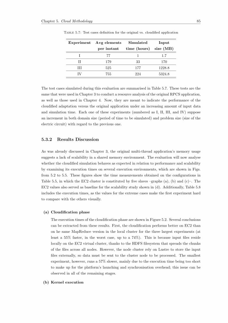
Chapter 5. Cloud Methodology 85
Table 5.7: Test cases definition for the original vs. cloudified application
Experiment Avg elements Simulated Input
per instant time (hours) size (MB)
I 77 1 1.7
II 179 33 170
III 525 177 1228.8
IV 755 224 5324.8
The test cases simulated during this evaluation are summarised in Table 5.7. These tests are the
same that were used in Chapter 3 to conduct a resource analysis of the original RPCS application,
as well as those used in Chapter 4. Now, they are meant to indicate the performance of the
cloudified adaptation versus the original application under an increasing amount of input data
and simulation time. Each one of these experiments (numbered as I, II, III, and IV) suppose
an increment in both domain size (period of time to be simulated) and problem size (size of the
electric circuit) with regard to the previous one.
5.3.2 Results Discussion
As was already discussed in Chapter 3, the original multi-thread application’s memory usage
suggests a lack of scalability in a shared memory environment. The evaluation will now analyse
whether the cloudified simulation behaves as expected in relation to performance and scalability
by examining its execution times on several execution environments, which are shown in Figs.
from 5.2 to 5.5. These figures show the time measurements obtained on the configurations in
Table 5.5, in which the EC2 cluster is constituted by five slaves –graphs (a), (b) and (c)–. The
EC2 values also served as baseline for the scalability study shown in (d). Additionally, Table 5.8
includes the execution times, as the values for the extreme cases make the first experiment hard
to compare with the others visually.
(a) Cloudification phase
The execution times of the cloudification phase are shown in Figure 5.2. Several conclusions
can be extracted from these results. First, the cloudification performs better on EC2 than
on he same MapReduce version in the local cluster for the three largest experiments (at
least a 55% faster, in the worst case, up to a 74%). This is because input files reside
locally on the EC2 virtual cluster, thanks to the HDFS filesystem that spreads the chunks
of the files across all nodes. However, the node cluster rely on Lustre to store the input
files externally, so data must be sent to the cluster node to be processed. The smallest
experiment, however, runs a 57% slower, mainly due to the execution time being too short
to make up for the platform’s launching and synchronisation overhead; this issue can be
observed in all of the remaining stages.
(b) Kernel execution


Chapter 5. Cloud Methodology 89
general methodology to transform simulations into a highly scalable MapReduce application
that re-uses the same simulation kernel while distributing the simulation load across as many
nodes are desired in a virtual cluster running on the cloud.
The procedure requires an application analysis phase in which at least one independent variable
must be found, since this element will act as index for the cloudification phase. The cloud
adaptation stage transforms the original input into a set of partitions indexed by the the previous
variable by means of a MapReduce job; these partitions are fed to a second MapReduce job that
executes the simulation kernel independently for each, merging the final results as well.
This methodology performs a paradigm shift from resource-bound applications to a data-centric
model; such cloudification mechanism provides effective cloud migration of simulation kernels
with minimal impact on the original code and achieves great scalability since limiting factors
are scattered. The promising results obtained in the particular use case studied, in terms of
performance and scalability, support the model’s viability. Moreover, we think that this cloudifi-
cation methodology may improve its results on parameter sweep problems, due to its pleasingly
parallel pattern and the benefit from data locality on such kind of problems. The results of
the methodology on multivariate analysis through parameter sweep will be studied in the next
chapter.


Chapter 6
Multivariate Analysis of
Simulation Problems
In the previous chapter, a methodology to transform simulations into a highly scalable MapRe-
duce application has been proposed. Up to this point, the methodology focuses on splitting a
single simulation into multiple tasks that use the same simulation kernel, distributing the simu-
lation load across as many nodes are desired. Nevertheless, modern workflows that make use of
simulation tools usually perform not one but many simulations, in the context of MOO problems,
parameter sweep applications, or rapid prototyping.
This chapter focuses on extending the proposed methodology to include multivariate analysis
simulations, as a particular case of pleasingly parallel problem. The kinds of applications that
benefit the most of this paradigm are the ones with many loosely coupled tasks, including those
simulations based on parameter sweep. Most simulators that fulfil the proposed enhancement
rely on several parameters to configure a specific experiment. All of these variables can be
changed independently, yielding an exponential number of possible experiments. This com-
plexity is further problematic if one decides to combine more than one variable at a time in
a multidimensional experiment analysis. Therefore, it is meaningful to consider multivariate
analysis within the methodology, thus providing a mechanism to execute concurrently a large
number of simulations in the same infrastructure.
6.1 Multivariate Analysis on Current Simulators
As computer systems have been evolved, the role of simulators have turned, from merely imitators
of the real world, to expert systems with the ability of taking decisions and complement the user
knowledge with metrics in order to achieve the best solutions. The main goal of a modern
simulator is not reduced to perform the simulation and output the results to the user. It has to
generate candidate solutions (experimental designs, prototypes, or models), evaluate if they are
acceptable or not, and provide a degree of fitness.
91

Chapter 6. Multivariate Analysis 92
This procedure is composed of several tasks: first, a candidate solution must be selected, either
being provided by the user, or being generated by the simulator itself. Then, the simulation
is performed and the results are analysed. The candidate solution is scored, and a decision to
accept it or reject it is taken. This procedure is repeated across all areas in which simulators are
used on. A simulator must not be restricted to evaluate solutions provided by the user, but also
it should find acceptable solutions by itself, with a high degree of fitness, and in a reasonable
amount of time.
6.1.1 Proposal of Simulation Enhancement
To achieve these targets an enhanced simulation structure is presented, which allows increasing
the output of simulators by covering more capabilities than the main procedure described before.
This enhancement is focused on four main issues which we proceed to describe.
• Layer 1: computing elasticity. First of all, modern simulators should be capable of taking
advantage of modern Cloud architectures, which can allocate computing resources upon
user request. Productivity issues in industry require to shorten the deadlines when evalu-
ating new designs. Besides, the design process may require evaluating a lot of candidate
solutions. We state that an efficient simulator should be adaptable to the underlying hard-
ware, so as to let the user to control the simulation times, allocating more computing
resources to shorten the deadlines, or giving up time if the computing resources are low.
• Layer 2: automatic generation and evaluation. In the second place, automatic generation
and simulation of solutions falls outside the scope of most simulators. Therefore, the
user must feed the simulator providing new possible solutions, which leads to productivity
losses. Moreover, the capacity of finding good (maybe optimal) solutions is tied to the
user and her own ability to explore the problems search space. We state that an efficient
simulator should evaluate and simulate a set of solutions with a minimal user involvement.
To achieve that: a) the user should provide the simulation parameters as a set of possible
values (e.g. [minimum, maximum, increment]), and the simulator uses them to generate
candidate solutions; b) the simulator should be able to generate new solutions starting
from an initial database (e.g. an inventory or catalogue).
• Layer 3: include stakeholders. Thirdly, there are many stakeholders taking part in the
design process which usually fall out of the scope of the simulation models. These parts
can influence, or even determine, the final acceptance of the candidate solutions [NHC13].
For instance, the set of possible solutions when looking for a valid design of a railway
portal frame, can be limited by the availability of constructive pieces in the company’s
inventory, and once found, a portal frame that stands could not be in compliance with
legal normative in certain countries. All issues that have to be considered throughout the
design process, but fall out the scope of the simulation model, should be also taken into
account when simulators generate and evaluate candidate solutions. This category includes
provider specifications, client requirements, technical security, legal normative and even
budget limitations. Different ways of including such restrictions in the simulation model


Chapter 6. Multivariate Analysis 94
when evaluating a candidate solution. Examples of such restrictions are availability of construc-
tive pieces in company’s inventory when proposing a design, or compliance with legal normative
when evaluating the proposed design. Finally, layer 4 represents the expert’s domain knowledge
that allows to obtain better solutions. Decision rules used to generate better candidate solutions,
or optimization metrics used to choose the best one, are included in this layer. This approach
improves the efficiency of the simulators by giving them the ability of searching for the best
solutions in the problem space. Obtained solutions will be fully-integrated with the different
actors of the design process, that have been included as a part of the structure proposed.
There are multiple examples of this trend in simulation techniques. In computational fluid
dynamics, an aerodynamic design of a new vehicle can be tested in order to analyze its efficiency.
In overhead contact line designs, structural behavior [NHAR13] of poles and portal frames are
evaluated, checking their feasibility [SGG+12]. In nuclear physics, different designs of BWR
reactors can be simulated to analyze different aspects such as efficiency, integrity, etc. In the
field of energy provisioning, a proposal of electric installation locations may be simulated checking
whether energy is available to all planned consumers [ASS13].
6.1.2 Cloud-Based Approach to Multivariate Analysis
The proposed structure allows to increase the output of the simulators, generating and evaluating
multiple solutions, and taking into account different parts of the design process. Nevertheless,
this theoretic approach have to be implemented and tested in order to make its advantages
effective. In Chapter 3 we stated that multivariate analysis can be described as a pleasingly
parallel problem, in which each simulation can be performed concurrently. We stated also that
Cloud platforms were the best-suited in order to deploy pleasingly parallel problems. Therefore,
we propose an approach to implement this structure in the Cloud.
• Regarding to issue 1, the system should have a flexible computing power which could
adapt to the computational complexity of the simulated domain. Complex simulations
may require more computing power to evaluate solutions, whereas simple simulations can
lead to untapped resources. The user should be capable of set the trade-off between time
and resources as desired, customizing the computational capacity of the infrastructure.
• Regarding to issue 2, the system should have a software engine which generates the specific
domain solutions. Starting from the domain description and simulation parameters, this
component should create a model of the solution, which will be simulated by a simulation
engine. Also, this component should be able to vary the simulation parameters (or the
simulation scenario) in order to generate different solutions and to explore the solutions
space.
• Regarding to issues 3 and 4, the system should have a database which contains all restric-
tions from stakeholders taking part in the design process, and all the optimization metrics
and heuristics that can influence the final acceptance of the solutions. Those factors must
be formalized and stored as decision rules.


Chapter 6. Multivariate Analysis 96
composed of decision rules databases. Generation and evaluation engines perform queries to
these databases when applying decision rules. Finally, the user interacts with the simulator
through a standard interface (e.g. web interface).
6.2 Methodology Enhancement for Multivariate Analysis
Since the methodology we described in Chapter 5 aims to provide task independence between
concurrent simulation partitions, we can perform a multivariate analysis by spawning several
simulations in a many-task manner. Many-task computing (MTC) is a new computing paradigm
that mixes high throughput computing (HTC) and high performance computing (HPC). Its main
goal is to make an efficient use of a large number of computing resources over short periods of
time to execute many computational tasks [RFZ08]. The main difference with HTC is that the
throughput is measured as tasks over very short periods of time –such as FLOPS, tasks/s, etc.–
instead of jobs per month, for instance.
Scientific simulations such as DNA database analysis, data processing in the Large Hadron
Collider (LHC) and climate modelling constitute examples of applications that make use of
many-tasks to analyse their huge amount of data. These applications rely on large quantities of
data, therefore data locality seems critical for large scale MTC. In fact, [RFZ08] states that data-
aware scheduling minimises data movement across nodes and benefits performance. Given this
context, it seems natural to enhance out data-centric methodology with a many-task deployment
to support multidimensional analysis, while enforcing efficient resource utilisation and balance.
In the Section 6.1.1, the advantages of developing simulators with an increased set of capabilities
have been exposed: not only simulating and evaluating scenarios provided by the user, but
also generating a new set of scenarios by its own, thus exploring the solution search space.
A simulator should also implement the evaluation function necessary to score the simulated
scenario, off-loading this task from the user. Combining these two properties, a third one arises,
since with a little additional development the simulator should be capable of conducting a guided
search for optimal solutions across the problem’s domain space.
Given this context, it seems natural to enhance out data-centric methodology with a many-task
deployment to support multivariate analysis, while enforcing efficient resource utilisation and
balance. The following sections describe, implement and evaluate a multivariate analysis tool,
implemented as a many-task deployment based on our cloudification methodology.
6.2.1 Multivariate Terms and Definitions
First of all, it is important to note that not one, but many simulations have to be performed, so
the Equation 5.1 evolves to Equation 6.1, that represents the concept of many simulations Si,
each one with its corresponding input data set Ii, and output data set Oi:
Si ≡ fsim(Ii) = Oi (6.1)

Chapter 6. Multivariate Analysis 97
Then, in order to include the multivariate analysis in the methodology, the following concepts
have to be added to those defined in Section 5.1.1:
• Generation engine. The function G ≡ fgen that, starting from an initial scenario I, gen-
erates derivative scenarios as variations of the initial one, performing modifications to the
input data set. This modifications can be performed through different ways: user-driven,
parameter sweep, evolutionary algorithms, etc.
G ≡ fgen(I, i) = Ii (6.2)
• Evaluation engine. The function E ≡ fev that process the output results from a simulation,
and gives a score for that scenario indicating its suitability, optimality, or any other quality
indicator θ related to the simulation domain.
E ≡ fev(Oi) = θi (6.3)
The aim is to find the scenario Ik that maximizes the score obtained from that evaluation
function, after evaluating the whole set of considered scenarios:
Ik | θk = max∀x
θx (6.4)
The evaluation engine can be expressed as the union of two different sets of evaluating
conditions that influence the validity and optimality of the solution in different ways:
restrictions rules fres, and optimization metrics fopt.
fev(Oi) = fres(O
i) · fopt(Oi) (6.5)
• Restriction rules. The restriction rules fres are those evaluating conditions whose fulfilment
is mandatory in order to consider a solution valid to the problem domain. These rules do
not consider the optimality of the solution, only if it meets the minimum requirements. As
result, the image of fres is binary: 1 if fulfilled, 0 if not. Due to the fact that every and
each of the restrictions rules must be satisfied in order to consider the solution valid, fres
is expressed as the product of each one of the functions f ires which corresponds to each
evaluation rule.
fres(Oi) = f1
res(Oi) · f2
res(Oi) · f3
res(Oi) · ... · fn
res(Oi) (6.6)
f ires : O
i → 0, 1 (6.7)
• Optimization metrics. The evaluation rules fopt are those evaluating conditions that in-
dicate a degree of quality associated to the problem domain, so provided the set of valid
solutions, they can be used to tell apart the good solutions from the bad ones. In order
to score the optimality of a solution, the output of these functions is a real number, and

Chapter 6. Multivariate Analysis 98
the objective is to find the maximum (or minimum) value associated to the best solution
across the simulated ones. If some optimization metrics have more impact than others in
the problem domain, each metric f iopt can be weighted using a coefficient ωi which helps
to determine the influence on the metric i within the whole set of optimization metrics.
fopt(Oi) = f1
opt(Oi) · ω1 + f2
opt(Oi) · ω2 + f3
opt(Oi) · ω3 + ...+ fn
opt(Oi) · ωn (6.8)
f iopt : O
i → R (6.9)
ωi ∈ R (6.10)
• Search engine. The search engine defines the global strategy for exploring the problem
space. While the generation engine is accountable for providing new scenarios, and the
evaluation engine gives a score to that scenarios after the simulations, the search engine
establishes how many simulations will be generated, what will be the seed for the genera-
tion, how many simulations will be performed simultaneously, how the evaluation results
will influence the search, etc. A BFS, an A*, or evolutionary algorithms are examples of
search engines that make use of the generation and evaluation engines to proceed with the
exploration of the problem space.
• Population. This concept is strongly related to the search engine, but it is defined apart
due to its relevance in terms of performance and efficiency. The population establishes
how many simulations can be performed in the same lot, i.e. the maximum number of
scenarios whose absence of dependences between them allows to conduct their simulations
simultaneously. This means that the score of a particular scenario does not influence the
possibility of conducting the simulation of any other of the same lot. The meaning is
the same as the population concept of genetic algorithms, where a set of individuals are
created, simulated, and evaluated all together, but applied also to other search algorithms
where it is possible to conduct several steps simultaneously.
In order to establish a multivariate analysis problem, the generation engine G and the evaluation
engine E should be defined, including all restriction rules, optimization metrics, and weights that
constitute E. Besides, the global search engine should be determined by deciding what is the
best strategy to explore the problem space. The population can be determined together with
the search engine, but it may also be influenced by how much resources are available in the
infrastructure.
6.2.2 Cloudification Process with Multivariate Enhancement
In order to enhance our methodology implementing the many-task programming paradigm, we
added some elements to the methodology structure proposed in Figure 5.1. This enhancement is
represented in Figure 6.3. The idea behind the figure is to wrap the adaptation and simulation


Chapter 6. Multivariate Analysis 100
Second, we run multiple map-reduce jobs, since we are simulating several scenarios concur-
rently. Note that, since multiple map-reduce jobs can be on execution at the same time,
the task scheduling has a potential impact on performance across the global workload.
• Scenario generator and evaluator. We propose that an efficient simulator should evaluate
and simulate a set of solutions with a minimal user involvement. New generation sim-
ulators should be capable of proposing and evaluating new designs based on a range of
possible parameters. Besides, generating new scenarios to be evaluated allows us to deploy
the many-task paradigm in an easy way, with minimal user involvement. The proposed
methodology aims these objectives through two new components: a scenario generator and
an evaluator. We define scenarios as independent simulations, each one of them with a
different input data set (though parts, or even almost of the data can be similar), that
have to be evaluated separately. Varying the input data leads to a different scenario (e.g.
a different infrastructure to be evaluated, or different environmental conditions the current
infrastructure have to be checked with).
The scenario generator and the evaluator wrap the simulation model (i.e. the adapta-
tion and simulation phases) generating different solutions to be evaluated. The scenario
generator creates new scenarios through variations in the input data, thus allowing ex-
perimentation with different simulation parameters, components or domain restrictions.
Those scenarios are provided to the map-reduce cluster, which performs the simulation as
described in the Section 5.1.3. The evaluator analyses the output from that simulations
and scores the generated solutions, stating whether they are acceptable or providing a
measure of their quality.
• Search engine. In order to conduct the search across the problem space, it is necessary a
component which implements a strategy defining the number and timing the scenarios are
created and evaluated. This strategy can take the form of BFS, DFS, genetic algorithms,
etc. and decides how many scenarios compound the population, how to guide the successive
evolutions, how is the global progress of the search, when to stop searching, etc.
• Scheduling and coordination Due to the fact that multiple simulations are going to be
executed in the cluster, it is necessary an management component which could act as
resource manager. Some platforms do have a resource manager which can schedule the tasks
efficiently (e.g. YARN on Hadoop MR), but others may lack of an adequate manager, so it
should be implemented externally. This is accountable for deciding how many simulations
will compound the batch of tasks be dispatched to the map-reduce cluster. The number
of tasks executed concurrently in the cluster (population) is a crucial parameter in terms
of performance and efficiency. An excessive number of tasks may lead to the saturation
of the cluster resources, whereas an insufficient number of tasks may lead to resource
underutilization.
Generating and evaluating multiple scenarios automatically allows a simulator to try different
solutions, thus providing a faster way of exploring the solution space. Rather than obtaining
a single solution, this method obtains a set of feasible solutions from which the user can select
the best one. Moreover, advanced search algorithms may be implemented. For instance, the

Chapter 6. Multivariate Analysis 101
generator. the evaluator, and the search engine could implement a guided search using heuristics
in order to find an optimal solution.
Algorithm 9 Multivariate engine: generation, simulation, and evaluation of multiple solutions
Input: I0, n, schedulerOutput: Bests1: i← 0 ⊲ Initialize variables2: j ← 03: Bests← ∅4: while !stopCondition do ⊲ Until the users decides to stop searching5: i← j6: for (i < j + n) do ⊲ Generate child solutions from the initial scenario7: Ii ← Generate(I0, i)8: i← i+ 19: end for
10:
11: i← j ⊲ Dispatch adaptation phases (Map-Reduce tasks)12: for (i < j + n) do13: Wait(scheduler.Allows)14: {Iiglob, I
i0, I
i1, I
i2, I
i3, ...I
ik} ← Dispatch(AdaptationPhase, Ii)
15: i← i+ 116: end for17:
18: Wait(scheduler.AllF inished)19:
20: i← j ⊲ Dispatch simulation phases (Map-Reduce tasks)21: for (i < j + n) do22: Wait(scheduler.Allows)23: Oi ← Dispatch(SimulationPhase, {Iiglob, I
i0, I
i1, I
i2, I
i3, ...I
ik})
24: i← i+ 125: end for26:
27: Wait(scheduler.AllF inished)28:
29: i← j30: for (i < j + n) do ⊲ Evaluate and score results31: θi ← Evaluate(Oi)32: i← i+ 133: end for34:
35: Bests← Bests ∪ Ik | θk = maxj≤i≤j+n
θi ⊲ Get the best solutions from those evaluated36: j ← i37: end while
Algorithm 9 illustrates the pseudocode of a very basic search engine using the proposed method-
ology. The algorithm starts from three input parameters: an initial test case I used as base for
generating new scenarios, and a population number n, used to establish how many simulations
will compound the batch of tasks, and an scheduler object, either implemented by the user or
provided by the platform, which acts as cluster resource manager.
While the stop condition is not reached (either established by the user or implemented through
a decision rule), the algorithm generates child solutions from the initial scenario using the gen-
eration engine. An ordinal is provided in order to evolve the generations as more scenarios are
created. Then, adaptation phases are dispatched in order to adapt those scenarios, following

Chapter 6. Multivariate Analysis 102
the same algorithms proposed in Chapter 5. Nevertheless, this stage can be optimized, reducing
replication in those scenarios which share part of the input data. Thus, the number of generation
stages can be lower than the number of simulations.
After the adaptation, the simulation tasks are dispatched to the cluster, performing concurrently
among the cluster. This leads to an optimal use of cluster resources, where multiple map-reduce
tasks are scheduled and executed so their phases can be interleaved. As the simulation tasks are
finishing, the results can be evaluated using the evaluation engine. The aim is to find the bests
solutions of those evaluated. In this case, the best of each bunch executed concurrently is added
to the set of best solutions.
The scheduler acts as semaphore deciding whether or not there are available resources on the
cluster. It has a direct impact on the cluster performance, being a trade-off between workload
overhead (if we have too many simulations running) and waste of resources (if we have too few),
so it should be implemented carefully.
There are different alternatives to the workflow shown in Algorithm 9. The best solutions can
act as base cases for the next iterations, following a pattern commonly displayed on evolutionary
algorithms. Besides, optimal solutions can be separated from the set of valid ones, in order to
implement elitism or any other technique.
6.3 Case study: RPCS
The cloudified application selected to perform the multidimensional analysis was the railway elec-
tric power consumption simulator presented in Chapter 3. We have implemented an enhancement
to the RPCS basic structure, turning towards a MOO problem. In this MOO problem, not one,
but many simulations will be executed. Each one of these simulations constitutes a variation of
the input data –either the infrastructure or the trains–, and the results are evaluated according
to a set of optimisation metrics in order to find the optimum initial configuration, with regard
to a specific optimisation criteria. The way we vary the input data defines the problem’s search
space, which constitutes the set of solutions obtained from the simulations, and the optimisation
metrics and functions define the goal we pursue in our search.
The problem search space to be studied will be the placement of the electrical substations
along the tracks –i.e. the connection milemarker of the substation to the track–. By modifying
the substations’ locations, we vary the electric circuit, thus we obtain different measures of
instantaneous and mean voltages, as well as consumed potency. Therefore, substation placement
has a direct impact on the power supply quality and energy savings.
In this particular case, we focus on the trade-off between energy saving and quality of energy
provisioning. The quality of the power supply refers to the concept of maintaining the system
as near to the nominal voltage, Unom = 3000V , as possible. As trains circulate along the tracks
demanding power, voltage oscillations may arise all across the electric circuit, leading to voltage
drops or over-voltages. Note that trains do not always consume the same amount of power,
and even more, they can return power to the circuit due to regenerative braking technologies.


Chapter 6. Multivariate Analysis 104
Pk =Ekfin
− Ekini
∆k
(6.11)
The generation engine should vary the positions of the substations progressively, and according
to their corresponding intervals as more derivative scenarios are created, so the function is defined
as follows.
G ≡ fgen(I, i, k) =
Ek = Ekini+ i mod Pk, if k = 1
Ek = Ekini+ i
Ek−1fin−Ek−1ini
∆k−1
mod Pk, if k = 2
Ek = Ekini+ i
(
Ek−1fin−Ek−1ini
∆k−1·Ek−2fin
−Ek−2ini
∆k−2
) mod Pk, if k = 3
(6.12)
where i, is the number of the i-th generated scenario, and k is the number of the k-th substation
which is going to be placed.
As each substation can be assigned to any of the points within the former interval, and all of
the substations have to be combined with the others to generate the experiment set, we would
get as many different experiments as indicated by Equation 6.13, where M is the number of
substations to be manipulated. The equation indicates that, the finer the grain of the planned
experiments, the more simulations have to be executed in order to generate the solution space.
n =M∏
k=1
Pk (6.13)
For this evaluation, we generated a set of 4 000 solutions using the variations of the positions indi-
cated in Table 6.1, displacing each substation from one kilometre to the next, without overlapping
their ranges. From this set, we sampled for this evaluation only 1 000 random experiments as
population, aiming to increase this number for future works. Note that, since each experiment
is composed of 4 800 simulation steps –one per simulated instant, corresponding to 1h and 20m
of simulated time–, it would be required to solve 4 800 equation systems per experiment. The
search engine implements a basic BFS algorithm, in which we first evaluate all variations of the
first substation, then we combine all these variations with variations of the second substation,
and so on. Algorithm 10 illustrates the basic code for the generation of cases.
Algorithm 10 BFS multivariate engine implemented on the top the RPCS
1: i← 02: for (i < 4000) do3: Ii ← Generate(I0, i, 1)4: Ii ← Generate(Ii, i, 2)5: Ii ← Generate(Ii, i, 3)6: i← i+ 47: end for

Chapter 6. Multivariate Analysis 105
6.3.2 Problem Formalisation: Evaluation Engine
As previously described, there are two objectives that guide the optimisation process:
• Improving the quality of the power supply.
• Reducing the amount of power consumed by the groups.
We define from these goals the following criteria:
• Maximise the mean useful voltage per train, f1opt.
• Minimise total amount of energy consumed by the groups, f2opt.
The mean useful voltage, described in European normative UNE-EN-50388 [CEN12], is defined
as the mean of all voltages at the pantograph of each train in the geographic zone, along all
simulation steps. This measure indicates the quality of the power supply. The lower the mean
useful voltage is, the less energy is transferred from the supply stations to the trains, on average.
For the formalisation of this problem, let T be the set of trains in the whole system, and G be
the set of groups in the network. The first objective is defined in Equation 6.14, where U tmu is
the mean useful voltage per train, and Umax1constitutes the maximum permanent voltage.
max f1opt =
U tmu − 2800
Umax1− 2800
∀t ∈ T (6.14)
The second objective is formulated in Equation 6.15, where Eig is the energy consumed per group,
in kW/h.
min f2opt =
G∑
i=1
Eig i 6= g, ∀g ∈ G (6.15)
As said before, the aim to find the corresponding Pareto frontier of the MOO problem, so no
combination of both metrics will be performed, and no weights ω1 and ω2 will be used to modify
such metrics. The problem is subject to the following constraints:
• According to the normative [CEN12], the mean useful voltage per train, U tmu, must never
be lower than 2800V , and it shall not surpass the maximum permanent voltage, Umax1.
f1res ≡ 2800 ≤ U t
mu ≤ Umax1(6.16)
• No sharp voltage drops or over-voltages shall exist on normal (non failure) operating condi-
tions [AEN04]. Therefore, instantaneous voltages should be in the range of non-permanent
conditions on every instant of the simulation. This derives Equation 6.17a and Equation
6.17b.
f2res ≡ Umin1
≤ Ut ≤ Umax2∀t ∈ T (6.17a)
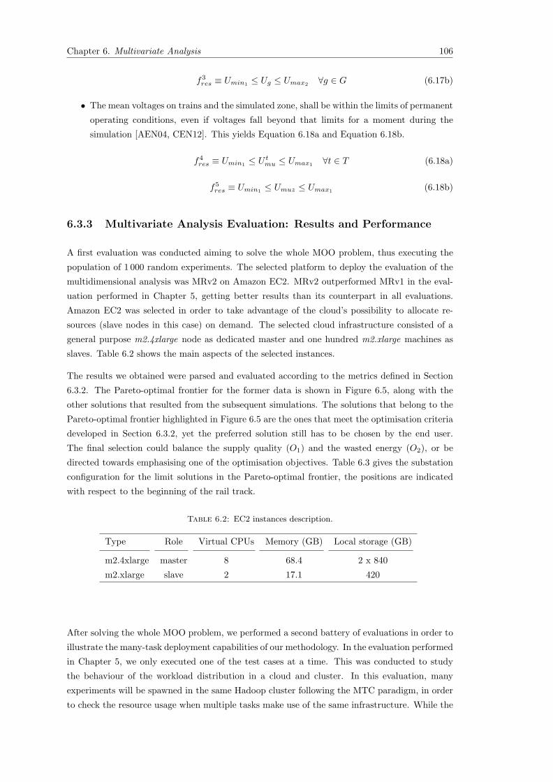
Chapter 6. Multivariate Analysis 106
f3res ≡ Umin1
≤ Ug ≤ Umax2∀g ∈ G (6.17b)
• The mean voltages on trains and the simulated zone, shall be within the limits of permanent
operating conditions, even if voltages fall beyond that limits for a moment during the
simulation [AEN04, CEN12]. This yields Equation 6.18a and Equation 6.18b.
f4res ≡ Umin1
≤ U tmu ≤ Umax1
∀t ∈ T (6.18a)
f5res ≡ Umin1
≤ Umuz ≤ Umax1(6.18b)
6.3.3 Multivariate Analysis Evaluation: Results and Performance
A first evaluation was conducted aiming to solve the whole MOO problem, thus executing the
population of 1 000 random experiments. The selected platform to deploy the evaluation of the
multidimensional analysis was MRv2 on Amazon EC2. MRv2 outperformed MRv1 in the eval-
uation performed in Chapter 5, getting better results than its counterpart in all evaluations.
Amazon EC2 was selected in order to take advantage of the cloud’s possibility to allocate re-
sources (slave nodes in this case) on demand. The selected cloud infrastructure consisted of a
general purpose m2.4xlarge node as dedicated master and one hundred m2.xlarge machines as
slaves. Table 6.2 shows the main aspects of the selected instances.
The results we obtained were parsed and evaluated according to the metrics defined in Section
6.3.2. The Pareto-optimal frontier for the former data is shown in Figure 6.5, along with the
other solutions that resulted from the subsequent simulations. The solutions that belong to the
Pareto-optimal frontier highlighted in Figure 6.5 are the ones that meet the optimisation criteria
developed in Section 6.3.2, yet the preferred solution still has to be chosen by the end user.
The final selection could balance the supply quality (O1) and the wasted energy (O2), or be
directed towards emphasising one of the optimisation objectives. Table 6.3 gives the substation
configuration for the limit solutions in the Pareto-optimal frontier, the positions are indicated
with respect to the beginning of the rail track.
Table 6.2: EC2 instances description.
Type Role Virtual CPUs Memory (GB) Local storage (GB)
m2.4xlarge master 8 68.4 2 x 840
m2.xlarge slave 2 17.1 420
After solving the whole MOO problem, we performed a second battery of evaluations in order to
illustrate the many-task deployment capabilities of our methodology. In the evaluation performed
in Chapter 5, we only executed one of the test cases at a time. This was conducted to study
the behaviour of the workload distribution in a cloud and cluster. In this evaluation, many
experiments will be spawned in the same Hadoop cluster following the MTC paradigm, in order
to check the resource usage when multiple tasks make use of the same infrastructure. While the


Chapter 6. Multivariate Analysis 110
domain, and decision rules to implement domain specific knowledge (restrictions, optimization
metrics). This allows to keep the design aware of specific domain data. The user can define
the simulation model as well as the rules in which are based both evaluation and optimization
functions. The Cloud infrastructure bring us the possibility of scale up or down the computing
resources according to the particular needs of the simulation.
Since the methodology we described in Chapter 5 aims to provide task independence between
concurrent simulation partitions, we can perform a multidimensional analysis by spawning several
simulations in a many-task manner. Given this context, it seems natural to enhance out data-
centric methodology with a many-task deployment to support multidimensional analysis, while
enforcing efficient resource utilisation and balance. Our evaluations indicate that the enhanced
system scales linearly with the number of experiments for every cluster size tested. This suggests
that the proposed methodology is suitable for multidimensional analysis via MTC, as we can run
several interleaved heterogeneous tasks making an efficient use of the infrastructure’s resources.
Furthermore, we can see that linearity is not loss in any case, so the end user can run the many-
task job successfully with either a few nodes or a larger infrastructure. This permits to tailor
the underlying infrastructure to reduce of economical costs or provide higher performance.

Chapter 7
Conclusions
In this thesis, we have analysed the suitability of performing simulations in clouds by performing
a paradigm shift, from classic parallel approaches to data-centric models, more adequate to be
executed on Cloud Computing infrastructures. We aimed to maintain the scalability achieved
in traditional HPC infrastructures while we take advantage of Cloud features. We have fulfilled
the objectives presented in Section 1.3:
O1 To explore the simulator’s characteristics that make them suitable or unsuitable to be de-
ployed on HPC or Cloud infrastructures. In Chapter 3, we characterize the different prob-
lem types that can be faced when working with simulators. This characterization is based
on the ease of splitting the problem in order to perform the computation in parallel. The
way we decompose the problem has a direct impact on data and communication patterns,
and should be studied carefully according to the target infrastructure and platform. We
also stated that several problem types can coexist in the same simulator, insofar as several
parallelizations can be applied to different layers of that simulator.
O2 To propose a methodology to adapt scientific simulations following a cloud-suitable data-
centric scheme, while maintaining classic approaches to domain decomposition for those
problems which cannot be split gracefully. In Chapter 5, we propose a general methodol-
ogy to transform simulations into a highly scalable MapReduce application that re-uses
the same simulation kernel while distributing the simulation load across as many nodes
are desired in a virtual cluster running on the cloud. The results show how the cloudfied
simulator outperforms the original multi-threaded application in Cloud infrastructures of
computing power similar to a single-node environment. Besides, we break the barrier be-
tween shared-memory environments and distributed memory environments, thus allowing
us to increase the number of nodes as we demand more computing power. Nevertheless,
the speed-up of the cloudified application is not as good as it would be desirable as this
number of nodes is increased but the problem size remains constant. In that case, the
problem size becomes small for the cluster size and less data is assigned to each slave. This
results in degraded performance due to platform overhead.
111

Chapter 7. Conclusions 112
O3 To transform a memory-bound simulator into the proposed scheme, integrating the original
application with both the MapReduce framework and MPI libraries. In Chapter 3, the
RPCS is introduced, as an example of memory-bound simulator. With the aim of serving
as case study, this simulator is analysed from the point of view described before, pointing
the different layers where opportunities for applying parallelization lie. In Chapter 4, the
RPCS is parallelized following classic HPC approaches based on MPI, thus proposing and
solving a tightly coupled problem. In Chapter 5, we apply the proposed methodology to
the RPCS, and explore the performance of changing to a data-centric approach based on
MapReduce.
O4 To demonstrate the feasibility of the resulting architecture comparing the behaviour and
efficiency of adapted vs. original applications in both HPC and Cloud environments. Mea-
surements and evaluations are conducted both in Chapter 4 and Chapter 5. In Chapter 4
we measure the performance of HPC approaches based on MPI, on both cluster and Cloud
environments. In Chapter 5, we measure the performance of the cloudified application
based on MapReduce, on both cluster and Cloud environments. The results show in that
Chapter 4 how the domain decomposition is the best approach in order to avoid communi-
cations, and the shortages of these MPI-based approaches in terms of fault tolerance and
stability. In Chapter 5, the promising results we got in the particular use case studied, in
terms of performance and scalability support, our initial model’s viability.
O5 To enhance the proposed methodology in order to include multivariate analysis simulations,
as a particular case that can benefit from a cloud-suitable data-centric scheme. In Chapter
6, we have proposed a enhanced simulation structure in order to bring to current simulators
multidimensional analysis, which allows increasing the output by covering more capabil-
ities than the main procedure. Since the methodology we described in Chapter 5 aims
to provide task independence between concurrent simulation partitions, we can perform a
multidimensional analysis by spawning several simulations in a many-task manner. Our
evaluations indicate that the enhanced system scales linearly with the number of experi-
ments for every cluster size tested. This suggests that the proposed methodology is suitable
for multidimensional analysis via MTC, as we can run several interleaved heterogeneous
tasks making an efficient use of the infrastructure’s resources.
Nowadays, HPC and Cloud Computing are two communities separated one from the other, and
they diverge in their research lines and objectives proposed. HPC community focus on breaking
the exascale barrier by developing more and more powerful infrastructures, and taking the max-
imum performance of such systems in all dimensions (processing, networking, energy efficiency,
etc.). On the contrary, Cloud Computing model is more focused on enterprises and business
world, bringing the users (no matter what type of user) the possibility of sizing computing com-
puting power according to instantaneous needs, at the expense of some performance loss. This
thesis explores the opportunities of establishing some common areas between both communities,
studying when and how HPC applications (such as simulators) can be deployed on Clouds, and
what are the advantages that Cloud Computing can bring to HPC community.

Chapter 7. Conclusions 113
7.1 Contributions
This thesis makes the following contributions:
C1 Classification of simulation problems according to its suitability to HPC and cloud infras-
tructures and the different ways of parallelizing such problems. First, we define what are
the key advantages on cluster on Cloud infrastructures, analyzing the performance in such
systems in terms of processing power, network, file systems, storage, etc. Then, we de-
fine three types of problems according to the structure and dependences between its data:
pleasingly parallel, loosely coupled, and tightly coupled problems. We state that a simula-
tion may expose several of these problems, depending on the level you apply parallelization.
Finally, we analyze what is the most suited type of infrastructure for each kind of problem.
C2 Proposition of different mechanisms to split simulation domains in smaller sub-domains,
with different degrees of data coupling, thus indicating the suitability of the simulator to
different infrastructures, identifying architectural bottlenecks, and those aspects which limit
the scalability of the application. We explore domain decomposition and matrix decom-
position as mechanisms to parallelize simulations in cluster environments using MPI. We
propose domain decomposition as mechanism to parallelize simulations in Cloud envi-
ronments, using MapReduce and the proposed Methodology. Finally, we propose using
MapReduce and the proposed Methodology in order to perform multivariate analysis on
Cloud environments.
C3 Definition of a software framework suitable for both cloud and HPC systems, that makes
use of data-centric schemes such as MapReduce. We propose a software framework based
on MapReduce as a part of the methodology proposed. The framework consists of two
MapReduce tasks. The adaptation task rearranges the input data set into multiple inde-
pendent subsets of global and domain data. The simulation task runs the simulation kernel
for each multiple independent subset that was mapped to them in the previous stage, plus
the required simulation parameters that are shared by every partition, so as reducers are
able to gather all the output and provide final results as the original application. Finally,
we enhance this software framework in order to conduct multidimensional analysis simu-
lations, dispatching several concurrent simulations following a many-task paradigm, and
taking further advantage of the Hadoop cluster resources.
C4 Implementation of the mechanisms and frameworks proposed in a simulator, and perfor-
mance study when different computing resources (e.g. HPC and cloud) are used. We
implement MPI version of the studied simulator, performing both domain and matrix de-
composition. We also migrate the simulator to Cloud using the methodology described,
obtaining promising results. Finally, we also implement multivariate analysis within the
simulator using the methodology described, obtaining linear scalability with the number
of experiments for every cluster size tested.

Chapter 7. Conclusions 114
7.2 Future Work
The work described in this thesis could be further extended and improved in many different
aspects. This section presents the future work derived from this thesis.
The first task to accomplish is to update the methodology, adapting it to novel frameworks like
Spark. Apache Hadoop is nowadays considered an obsolete platform, with performance issues
that have been solved in the last generation of data-centric frameworks. In particular, we are
considering other implementations to migrate to, such as Spark, that provide further functionality
and support for complex algorithms. Spark can help to improve the chained workflows like the
adaptation and simulation phases which constitute the basis of the methodology. Therefore, we
expect an improved performance if we adapt the algorithms and repeat the evaluations using
Spark.
Another research line is to explore approaches to execute tightly coupled problems in Clouds by
means of hierarchical decomposition. The thesis results have shown how sensible is the matrix
decomposition approach to the network latencies, even more if the size of the operated matrices
is not big enough to make the distributed parallel execution worthwhile. Therefore, domain
and matrix decomposition could be implemented simultaneously at different levels, for instance,
using domain decomposition to distribute workload across all nodes of the Cloud, and using
matrix decomposition to distribute workload across the CPU cores within the node, or using
small subsets of the Cloud nodes for matrix decomposition if the cores within the node are not
enough.
Future works are strongly focused on extending the current methodology to a generalized frame-
work which would allow to cloudify any scientific application, and conduct its execution in both
both HPC and Cloud infrastructures. This framework should make use of local cluster resources
if available, and allocate resources on cloud if the local resources are not enough. In order to
do so, domain and matrix decompositions should be mixed in order to avoid the impact of the
latencies between local and remote resources.
Finally, we aim to develop an interface for applications to make use of this framework. This
interface will represent the different types of problems and problem decompositions described
in this thesis, so as to develop applications in terms of domain, sub-domains, decompositions,
simulation kernels, etc. In this way, functional programming models like MapReduce could be
used, and more complicated communication patters like those present in the simulation kernels
could be hidden to the programmer.
7.3 Thesis Results
The main contributions of this thesis have been published in international conferences and jour-
nals. We enumerate the publications classified into journals, conferences, and workshops. Addi-
tionally, we indicate the research stays, grants, and projects related to the results of this thesis.
• Journals

Chapter 7. Conclusions 115
1. C. Gomez, R. Saa, A. Garcia, F. Garcia-Carballeira, and J. Carretero, ”A model
to obtain optimal designs of railway overhead knuckle junctions using simulation”,
Simulation Modelling Practice and Theory, vol. 26, pp. 16–31, August 2012. Impact
Factor: 0.969. Q2
2. R. Saa, A. Garcia, C. Gomez, J. Carretero, and F. Garcia-Carballeira, ”An ontology-
driven decision support system for high-performance and cost-optimized design of
complex railway portal frames”, Expert Systems with Applications, vol. 39(10), pp.
8784–8792, August 2012. Impact Factor: 2.203. Q1
3. A. Garcia, C. Gomez, R. Saa, F. Garcia-Carballeira, and J. Carretero, ”Optimizing
the process of designing and calculating railway catenary support infrastructure using
a high-productivity computational tool”, Transportation Research Part C: Emerging
Technologies, vol. 28, pp. 1–14, March 2013. Impact factor: 1.957. Q1
4. S. Caino-Lores, A. Garcia, F. Garcia-Carballeira, and J. Carretero, ”A cloudification
methodology for multidimensional analysis: Implementation and application to a rail-
way power simulator”, Simulation Modelling Practice and Theory, vol. 55, pp. 46–62,
June 2015. Impact factor: 1050. Q2
• Conferences
1. R. Saa, A. Garcia, C. Gomez, F. Garcia-Carballeira, and J. Carretero, ”A high-
productivity computational tool to model and calculate railway catenary support
structures”, in The 2012 International Conference of Computer Science and Engi-
neering, London, United Kingdom, July 2012. Best Student Paper Award.
2. A. Garcia, C. Gomez, F. Garcia-Carballeira, and J. Carretero, ”Enhancing the struc-
ture of railway infrastructure simulators”, in International Conference on Engineering
and Applied Sciences Optimization (OPT-i), Kos, Greece, June 2014.
3. J. Carretero, C. Gomez, A. Garcia, and F. Garcia-Carballeira, ”A holistic approach to
railway engineering design using a simulation framework”, in The 4th International
Conference on Simulation and Modeling Methodologies, Technologies and Applications
(SIMULTECH 2014), Vienna, Austria, August 2014.
4. A. Garcia, S. Caino-Lores, F. Garcia-Carballeira, and J. Carretero, ”A multi-objective
simulator for optimal power dimensioning on electric railways using cloud computing”,
in The 5th International Conference on Simulation and Modeling Methodologies,
Technologies and Applications (SIMULTECH 2015), Kolmar, France, July 2015.
• Workshops
1. S. Caino-Lores, A. Garcia, F. Garcia-Carballeira, and J. Carretero, ”A cloudifica-
tion methodology for numerical simulations”, in Euro-Par 2014: Parallel Processing
Workshop, Porto, Portugal, August 2014.
2. S. Caino-Lores, A. Garcia, F. Garcia-Carballeira, and J. Carretero, ”Breaking data
dependences in numerical simulations using Map-Reduce”, in XXV Jornadas de Par-
alelismo, Valladolid, Spain, September 2014.

Chapter 7. Conclusions 116
• Research stays
West University of Timisoara, under the supervision of Prof. Dana Petcu, from November
2014 to February 2015.
• Grants
– Convocatoria PIF UC3M 01-11112 de Personal Investigador en Formacion, PhD fully
granted (4 years), 2011, Universidad Carlos III de Madrid
– Programa propio de investigacion. Ayudas a la movilidad de investigadores en for-
macion predoctoral, 1050 e, 2014, Universidad Carlos III de Madrid.
• Bachelor thesis
– S. Caino-Lores. Adaptation, deployment and evaluation of a railway simulator in
cloud environments. Supervisor: Alberto Garcia. B.Sc in Computer Science. Univer-
sity Carlos III of Madrid. June, 2014. itSMF award to the best bachelor thesis.
• Projects
– Administrador de Infraestructuras Ferroviarias (ADIF), Estudio y realizacion de pro-
gramas de calculo de porticos rıgidos de catenaria (CALPOR) y de sistema de simu-
lacion de montaje de agujas aereas de lınea aerea de contacto (SIA), JM/RS 3.6/4100-
.0685-9/00100
– Administrador de Infraestructuras Ferroviarias (ADIF), Proyecto para la Investi-
gacion sobre la aplicacion de las TIC a la innovacion de las diferentes infraestructuras
correspondientes a las instalaciones de electrificacion y suministro de energa (SIRTE),
JM/RS 3.9/1500.0009/0-00000
– Spanish Ministry of Education, TIN2010-16497, Scalable Input/Output techniques
for high-performance distributed and parallel computing environments
– Spanish Ministry of Economics and Competitiveness, TIN2013-41350-P, Tecnicas de
gestion escalable de datos para high-end computing systems
– European Union, COST Action IC1305, ”Network for Sustainable Ultrascale Com-
puting Platforms” (NESUS)
– European Union, COST Action IC0805, ”Open European Network for High Perfor-
mance Computing on Complex Environments”
– Spanish Ministry of Economics and Competitiveness, TIN2011-15734-E, Red de Com-
putacion de Altas Prestaciones sobre Arquitecturas Paralelas Heterogeneas (CAPAP-
H)

Bibliography
[ABC+10] Steve Ashby, P Beckman, J Chen, P Colella, B Collins, D Crawford, J Dongarra,
D Kothe, R Lusk, P Messina, et al. The opportunities and challenges of exas-
cale computing. Summary Report of the Advanced Scientific Computing Advisory
Committee (ASCAC) Subcommittee (November 2010), 2010.
[Ade03] H. Adeli. Expert Systems in Construction and Structural Engineering. Taylor &
Francis, 2003.
[AEN04] AENOR. UNE-EN 50163: Railway Applications - Supply voltages of traction sys-
tems. AENOR, 2004.
[AFG+10] Michael Armbrust, Armando Fox, Rean Griffith, Anthony D. Joseph, Randy Katz,
Andy Konwinski, Gunho Lee, David Patterson, Ariel Rabkin, Ion Stoica, and Matei
Zaharia. A view of cloud computing. Commun. ACM, 53(4):50–58, April 2010.
[AK11] Dennis Abts and John Kim. High Performance Datacenter Networks: Architectures,
Algorithms, and Opportunities. San Rafael, California, 2011.
[AM13] Ismail Ari and Nitel Muhtaroglu. Design and implementation of a cloud computing
service for finite element analysis. Advances in Engineering Software, 6061(0):122
– 135, 2013.
[Ama] Amazon Elastic MapReduce (Amazon EMR). http://aws.amazon.com/es/
elasticmapreduce/. Last accessed Nov 2015.
[APK+12] M. AbdelBaky, M. Parashar, Hyunjoo Kim, K.E. Jordan, V. Sachdeva, J. Sexton,
H. Jamjoom, Zon-Yin Shae, G. Pencheva, R. Tavakoli, and M.F. Wheeler. Enabling
high-performance computing as a service. Computer, 45(10):72–80, 2012.
[Art13] Charles Arthur. Nsa scandal: what data is being monitored and how does it work?
The Guardian, Friday 7th June, 2013.
[ASS13] Lars Abrahamsson, Stefan stlund, Thorsten Schtte, and Lennart Sder. An elec-
tromechanical moving load fixed node position and fixed node number railway
power supply systems optimization model. Transportation Research Part C: Emerg-
ing Technologies, 30(0):23 – 40, 2013.
[Ban98] J. Banks. Handbook of Simulation: Principles, Methodology, Advances, Applica-
tions, and Practice. Wiley-Interscience publication. Wiley Online Library, 1998.
117

Bibliography 118
[BBC+08] Keren Bergman, Shekhar Borkar, Dan Campbell, William Carlson, William Dally,
Monty Denneau, Paul Franzon, William Harrod, Kerry Hill, Jon Hiller, et al. Ex-
ascale computing study: Technology challenges in achieving exascale systems. De-
fense Advanced Research Projects Agency Information Processing Techniques Office
(DARPA IPTO), Tech. Rep, 15, 2008.
[BCC+97] L. S. Blackford, J. Choi, A. Cleary, E. D’Azevedo, J. Demmel, I. Dhillon, J. Don-
garra, S. Hammarling, G. Henry, A. Petitet, K. Stanley, D. Walker, and R. C.
Whaley. ScaLAPACK Users’ Guide. Society for Industrial and Applied Mathe-
matics, Philadelphia, PA, 1997.
[BGDG+10] Andreas Berl, Erol Gelenbe, Marco Di Girolamo, Giovanni Giuliani, Hermann
De Meer, Minh Quan Dang, and Kostas Pentikousis. Energy-efficient cloud com-
puting. The computer journal, 53(7):1045–1051, 2010.
[BKK+09] Arthur S Bland, Ricky A Kendall, Douglas B Kothe, James H Rogers, and Galen M
Shipman. Jaguar: The worlds most powerful computer. In Proceedings of Cray User
Group, volume 300, page 362, 2009.
[Boa13] OpenMP Architecture Review Board. Openmp application program interface ver-
sion 4.0, Jul. 2013.
[Buy99] Rajkumar Buyya, editor. High Performance Cluster Computing: Architectures and
Systems. Prentice Hall, 1999.
[CBP00] L. Chwif, M.R.P. Barretto, and R.J. Paul. On simulation model complexity. In
Simulation Conference, 2000. Proceedings. Winter, volume 1, pages 449–455 vol.1,
2000.
[CBP+10] Navraj Chohan, Chris Bunch, Sydney Pang, Chandra Krintz, Nagy Mostafa, Sunil
Soman, and Rich Wolski. Appscale: Scalable and open appengine application devel-
opment and deployment. In DimiterR. Avresky, Michel Diaz, Arndt Bode, Bruno
Ciciani, and Eliezer Dekel, editors, Cloud Computing, volume 34 of Lecture Notes
of the Institute for Computer Sciences, Social-Informatics and Telecommunications
Engineering, pages 57–70. Springer Berlin Heidelberg, 2010.
[CDG+08] Fay Chang, Jeffrey Dean, Sanjay Ghemawat, Wilson C. Hsieh, Deborah A. Wallach,
Mike Burrows, Tushar Chandra, Andrew Fikes, and Robert E. Gruber. Bigtable:
A distributed storage system for structured data. ACM Trans. Comput. Syst.,
26(2):4:1–4:26, June 2008.
[CEN12] CENELEC. UNE-EN 50388: Railway Applications - Power supply and rolling
stock - Technical criteria for the coordination between power supply (substation)
and rolling stock to achieve interoperability. AENOR, 2012.
[CEN15] CENELEC. prEN 50641 (draft): Railway Applications - - Fixed installations -
Requirements for the validation of simulation tools used for the design of trac-
tion power supply systems. CENELEC: Europeean Committee for Electrotechnical
Standardization, 2015.

Bibliography 119
[CHA+11] P. Carns, K. Harms, W. Allcock, C. Bacon, S. Lang, R. Latham, and R. Ross.
Understanding and improving computational science storage access through con-
tinuous characterization. In Mass Storage Systems and Technologies (MSST), 2011
IEEE 27th Symposium on, pages 1–14, 2011.
[CJP+11] Carlo Curino, Evan Philip Charles Jones, Raluca Ada Popa, Nirmesh Malviya, Eu-
gene Wu, Samuel R Madden, Hari Balakrishnan, and Nickola Zeldovich. Relational
cloud: A database-as-a-service for the cloud. In Conference on Innovative Data
Systems Research, CIDR 2011, January 9-12, 2011 Asilomar, California, 2011.
[Cla12] Kelly Clay. Amazon aws takes down netflix on christmas eve. Forbes, 24th Decem-
ber, 2012.
[Clo14] The top 20 infrastructure as a service (iaas) vendors, July 2014. http://www.
clouds360.com/. Last accessed Nov 2015.
[CLZB00] Henri Casanova, Arnaud Legrand, Dmitrii Zagorodnov, and Francine Berman.
Heuristics for scheduling parameter sweep applications in grid environments. In
Heterogeneous Computing Workshop, 2000.(HCW 2000) Proceedings. 9th, pages
349–363. IEEE, 2000.
[CMPW12] Paolo Costa, Matteo Migliavacca, Peter Pietzuch, and Alexander L. Wolf. Naas:
network-as-a-service in the cloud. In Proceedings of the 2nd USENIX conference
on Hot Topics in Management of Internet, Cloud, and Enterprise Networks and
Services, Hot-ICE’12, pages 1–1, Berkeley, CA, USA, 2012. USENIX Association.
[Cou13] Rachel Courtland. The status of moores law: Its complicated. IEEE Spectrum,
Oct, 2013.
[CPGC+03] Jesus Carretero, Jose M Perez, Felix Garcıa-Carballeira, Alejandro Calderon, Javier
Fernandez, Jose D Garcıa, Antonio Lozano, Luis Cardona, Norberto Cotaina, and
Pierre Prete. Applying rcm in large scale systems: a case study with railway
networks. Reliability engineering & system safety, 82(3):257–273, 2003.
[CSA12] Cloud computing market maturity - study results. Technical report, Cloud Security
Alliance, ISACA, 2012.
[D’A11] G. D’Angelo. Parallel and distributed simulation from many cores to the public
cloud. In 2011 International Conference on High Performance Computing and
Simulation (HPCS), pages 14–23, July 2011.
[DG08] Jeffrey Dean and Sanjay Ghemawat. Mapreduce: simplified data processing on
large clusters. Communications of the ACM, 51(1):107–113, 2008.
[DL11] Jack Dongarra and Piotr Luszczek. Linpack benchmark. Encyclopedia of Parallel
Computing, pages 1033–1036, 2011.
[DMS+97] Jack J Dongarra, Hans W Meuer, Erich Strohmaier, et al. Top500 supercomputer
sites. Supercomputer, 13:89–111, 1997.

Bibliography 120
[dOOBM10] D. de Oliveira, E. Ogasawara, F. Baiao, and M. Mattoso. Scicumulus: A lightweight
cloud middleware to explore many task computing paradigm in scientific workflows.
In IEEE 3rd International Conference on Cloud Computing (CLOUD), pages 378–
385, July 2010.
[DWC10] T. Dillon, Chen Wu, and E. Chang. Cloud computing: Issues and challenges.
In 24th IEEE International Conference on Advanced Information Networking and
Applications (AINA), pages 27–33, April 2010.
[ECW10] Joseph Earl, Steve Conway, and Jie Wu. A new approach to hpc public clouds:
The sgi cyclone hpc cloud. Technical report, IDC, 2010.
[Edd10] Dirk Eddelbuettel. Benchmarking single-and multi-core blas implementations and
gpus for use with r, 2010.
[ELZ+10] Jaliya Ekanayake, Hui Li, Bingjing Zhang, Thilina Gunarathne, Seung-Hee Bae,
Judy Qiu, and Geoffrey Fox. Twister: A runtime for iterative mapreduce. In
Proceedings of the 19th ACM International Symposium on High Performance Dis-
tributed Computing, HPDC ’10, pages 810–818, 2010.
[EPF08] J. Ekanayake, S. Pallickara, and G. Fox. Mapreduce for data intensive scientific
analyses. In IEEE Fourth International Conference on eScience, pages 277–284,
Dec 2008.
[FC07] Wu-chun Feng and Kirk W Cameron. The green500 list: Encouraging sustainable
supercomputing. Computer, 40(12):50–55, 2007.
[FL05] Vincent W. Freeh and David K. Lowenthal. Using multiple energy gears in mpi
programs on a power-scalable cluster. In Proceedings of the Tenth ACM SIGPLAN
Symposium on Principles and Practice of Parallel Programming, PPoPP ’05, pages
164–173, New York, NY, USA, 2005. ACM.
[For15] Message Passing Interface Forum. Mpi: A message-passing interface standard ver-
sion 3.1, Jun. 2015.
[FQKYS04] Zhe Fan, Feng Qiu, Arie Kaufman, and Suzanne Yoakum-Stover. Gpu cluster for
high performance computing. In Proceedings of the 2004 ACM/IEEE Conference on
Supercomputing, SC ’04, pages 47–, Washington, DC, USA, 2004. IEEE Computer
Society.
[GALM07] Phillipa Gill, Martin Arlitt, Zongpeng Li, and Anirban Mahanti. Youtube traffic
characterization: A view from the edge. In Proceedings of the 7th ACM SIGCOMM
Conference on Internet Measurement, IMC ’07, pages 15–28, New York, NY, USA,
2007. ACM.
[GFB+04] Edgar Gabriel, Graham E Fagg, George Bosilca, Thara Angskun, Jack J Dongarra,
Jeffrey M Squyres, Vishal Sahay, Prabhanjan Kambadur, Brian Barrett, Andrew
Lumsdaine, et al. Open mpi: Goals, concept, and design of a next generation
mpi implementation. In Recent Advances in Parallel Virtual Machine and Message
Passing Interface, pages 97–104. Springer, 2004.

Bibliography 121
[GGGCC14] Alberto Garcıa, Carlos Gomez, Flix Garcıa-Carballeira, and Jess Carretero. En-
hancing the structure of railway infrastructure simulators. In Proceedings of the
1st International Conference on Engineering and Applied Sciences Optimization
(OPT-i), pages 352–363, 2014.
[GGS+13] Alberto Garcia, Carlos Gomez, Ruben Saa, Felix Garcia-Carballeria, and Jesus Car-
retero. Optimizing the process of designing and calculating railway catenary sup-
port infrastructure using a high-productivity computational tool. Transportation
Research Part C: Emerging Technologies, 28(0):1 – 14, 2013. Euro Transportation:
selected paper from the EWGT Meeting, Padova, September 2009.
[GL09] Al Geist and Robert Lucas. Major computer science challenges at exascale. In-
ternational Journal of High Performance Computing Applications, 23(4):427–436,
2009.
[Gre15] Green500 Organization. Green500 list, November 2015.
[GVDG08] Kazushige Goto and Robert Van De Geijn. High-performance implementation of
the level-3 blas. ACM Trans. Math. Softw., 35(1):4:1–4:14, July 2008.
[GWC+11] Thilina Gunarathne, Tak-Lon Wu, Jong Youl Choi, Seung-Hee Bae, and Judy
Qiu. Cloud computing paradigms for pleasingly parallel biomedical applications.
Concurrency and Computation: Practice and Experience, 23 (17):2338–2354, 2011.
[GWQF10] T. Gunarathne, Tak-Lon Wu, J. Qiu, and G. Fox. Mapreduce in the clouds for
science. In IEEE Second International Conference on Cloud Computing Technology
and Science (CloudCom), pages 565–572, Nov 2010.
[Hea11] Michael T Heath. Parallel numerical algorithms. Lecture Notes, Chapter 6:1–42,
2011.
[Hem10] Scott Hemmert. Green hpc: From nice to necessity. Computing in Science Engi-
neering, 12(6):8–10, Nov 2010.
[HH09] Z. Hill and M. Humphrey. A quantitative analysis of high performance comput-
ing with amazon’s ec2 infrastructure: The death of the local cluster? In 10th
IEEE/ACM International Conference on Grid Computing, pages 26–33, Oct 2009.
[HIM02] H. Hacigumus, B. Iyer, and S. Mehrotra. Providing database as a service. In 18th
International Conference on Data Engineering, 2002. Proceedings., pages 29–38,
2002.
[HMY+02] T.K. Ho, B.H. Mao, Z.Z. Yuan, H.D. Liu, and Y.F. Fung. Computer simulation and
modeling in railway applications. Computer Physics Communications, 143(1):1 –
10, 2002.
[Hoc94] Roger W. Hockney. The communication challenge for mpp: Intel paragon and
meiko cs-2. Parallel Computing, 20(3):389 – 398, 1994.

Bibliography 122
[IOY+11] A. Iosup, S. Ostermann, M.N. Yigitbasi, R. Prodan, T. Fahringer, and D.H.J.
Epema. Performance analysis of cloud computing services for many-tasks scientific
computing. EEE Transactions on Parallel and Distributed Systems, 22(6):931–945,
June 2011.
[ISO14] ISO/IEC. ISO/IEC 17788:2014 - Information technology - Cloud computing -
Overview and vocabulary. ISO/IEC, 2014.
[Jam12] Noreen Jamil. A comparison of direct and indirect solvers for linear systems of
equations. International Journal of Emerging Sciences, 2(2):310–321, 2012.
[JDV+09] G. Juve, E. Deelman, K. Vahi, G. Mehta, B. Berriman, B.P. Berman, and P. Maech-
ling. Scientific workflow applications on amazon ec2. In 5th IEEE International
Conference on E-Science Workshops, pages 59–66, Dec 2009.
[JMHJ] Stefan Jahn, Michael Margraf, Vincent Habchi, and Raimund Jacob. Qucs tech-
nical papers. http://qucs.sourceforge.net/tech/node14.html. Last accessed
November 2015.
[JRM+10] Keith R Jackson, Lavanya Ramakrishnan, Krishna Muriki, Shane Canon, Shreyas
Cholia, John Shalf, Harvey J Wasserman, and Nicholas J Wright. Performance
analysis of high performance computing applications on the amazon web services
cloud. In IEEE Second International Conference on Cloud Computing Technology
and Science (CloudCom), pages 159–168. IEEE, 2010.
[KES+09] Volodymyr V Kindratenko, Jeremy J Enos, Guochun Shi, Michael T Showerman,
Galen W Arnold, John E Stone, James C Phillips, and Wen-mei Hwu. Gpu clusters
for high-performance computing. In IEEE International Conference on Cluster
Computing and Workshops (CLUSTER’09), pages 1–8. IEEE, 2009.
[KPP09] Karthik Kambatla, Abhinav Pathak, and Himabindu Pucha. Towards optimizing
hadoop provisioning in the cloud. In Proc. of the First Workshop on Hot Topics in
Cloud Computing, page 118, 2009.
[KT11] V. Kindratenko and P. Trancoso. Trends in high-performance computing. Com-
puting in Science Engineering, 13(3):92–95, May 2011.
[Law08] G. Lawton. Developing software online with platform-as-a-service technology. Com-
puter, 41(6):13–15, June 2008.
[LBIC13] Pablo Llopis, Javier Garcia Blas, Florin Isaila, and Jesus Carretero. Survey of
energy-efficient and power-proportional storage systems. The Computer Journal,
2013.
[LCL+09] Samuel Lang, Philip Carns, Robert Latham, Robert Ross, Kevin Harms, and
William Allcock. I/O performance challenges at leadership scale. In Proceedings of
the Conference on High Performance Computing Networking, Storage and Analysis,
SC ’09, pages 40:1–40:12, New York, NY, USA, 2009. ACM.

Bibliography 123
[Lee10] Craig A. Lee. A perspective on scientific cloud computing. In Proceedings of the
19th ACM International Symposium on High Performance Distributed Computing,
HPDC ’10, pages 451–459, New York, NY, USA, 2010. ACM.
[LKC+10] Victor W. Lee, Changkyu Kim, Jatin Chhugani, Michael Deisher, Daehyun Kim,
Anthony D. Nguyen, Nadathur Satish, Mikhail Smelyanskiy, Srinivas Chennupaty,
Per Hammarlund, Ronak Singhal, and Pradeep Dubey. Debunking the 100x gpu
vs. cpu myth: An evaluation of throughput computing on cpu and gpu. SIGARCH
Comput. Archit. News, 38(3):451–460, June 2010.
[LO11] Huan Liu and Dan Orban. Cloud mapreduce: A mapreduce implementation on
top of a cloud operating system. In Proceedings of the 2011 11th IEEE/ACM
International Symposium on Cluster, Cloud and Grid Computing, pages 464–474.
IEEE Computer Society, 2011.
[Mah11] ZaighamMahmood. Cloud computing: Characteristics and deployment approaches.
In IEEE 11th International Conference on Computer and Information Technology
(CIT), pages 121–126, Aug 2011.
[MC03] Franco Maceri and Fabio Casciati. Modelling and simulation of advanced problems
and smart systems in civil engineering. Simulation Modelling Practice and Theory,
11(5-6):313 –, 2003. Modelling and Simulation of Advanced Problems and Smart
Systems in Civil Engineering.
[MCB+11] James Manyika, Michael Chui, Brad Brown, Jacques Bughin, Richard Dobbs,
Charles Roxburgh, and Angela H Byers. Big data: The next frontier for inno-
vation, competition, and productivity. McKinsey Global Institute, 2011.
[MG09] Peter Mell and Tim Grance. The nist definition of cloud computing. National
Institute of Standards and Technology, 53(6):50, 2009.
[MPI03] Mpich. a portable implementation of mpi, 2003. www.mcs.anl.gov/mpich2. Last
accessed Nov 2015.
[MWBA10] Richard C Murphy, Kyle B Wheeler, Brian W Barrett, and James A Ang. Intro-
ducing the graph 500. Cray Users Group (CUG), 2010.
[NHAR13] M. Nejlaoui, A. Houidi, Z. Affi, and L. Romdhane. Multiobjective robust design
optimization of rail vehicle moving in short radius curved tracks based on the
safety and comfort criteria. Simulation Modelling Practice and Theory, 30(0):21 –
34, 2013.
[NHC13] A. Naweed, G.R.J. Hockey, and S.D. Clarke. Designing simulator tools for rail re-
search: The case study of a train driving microworld. Applied Ergonomics, 44(3):445
– 454, 2013.
[NVI11] NVIDIA Corporation. NVIDIA CUDA C Programming Guide, June 2011.
[OHL+08] J.D. Owens, M. Houston, D. Luebke, S. Green, J.E. Stone, and J.C. Phillips. Gpu
computing. Proceedings of the IEEE, 96(5):879–899, May 2008.

Bibliography 124
[Ope11] OpenACC Working Group. The openacc application programming interface, 2011.
[ORS+08] Christopher Olston, Benjamin Reed, Utkarsh Srivastava, Ravi Kumar, and Andrew
Tomkins. Pig latin: A not-so-foreign language for data processing. In Proceedings
of the 2008 ACM SIGMOD International Conference on Management of Data,
SIGMOD ’08, pages 1099–1110, New York, NY, USA, 2008. ACM.
[PBB15] D. Pellerin, D. Ballantyne, and A. Boeglin. An introduction to high performance
computing on aws. Technical report, Amazon Web Services, August 2015.
[Pet11] Dana Petcu. Portability and interoperability between clouds: Challenges and case
study. In Witold Abramowicz, IgnacioM. Llorente, Mike Surridge, Andrea Zisman,
and Julien Vayssire, editors, Towards a Service-Based Internet, volume 6994 of
Lecture Notes in Computer Science, pages 62–74. Springer Berlin Heidelberg, 2011.
[PMPC13] Dana Petcu, Georgiana Macariu, Silviu Panica, and Ciprian Craciun. Portable
cloud applications, from theory to practice. Future Generation Computer Systems,
29(6):1417–1430, 2013.
[PO09] R. Prodan and S. Ostermann. A survey and taxonomy of infrastructure as a service
and web hosting cloud providers. In 10th IEEE/ACM International Conference on
Grid Computing, pages 17–25, Oct 2009.
[RBA11] A. Raveendran, T. Bicer, and G. Agrawal. A framework for elastic execution of
existing mpi programs. In Parallel and Distributed Processing Workshops and Phd
Forum (IPDPSW), 2011 IEEE International Symposium on, pages 940–947, 2011.
[RCL09] B.P. Rimal, Eunmi Choi, and I. Lumb. A taxonomy and survey of cloud computing
systems. In Fifth International Joint Conference on INC, IMS and IDC, 2009.
NCM ’09., pages 44–51, Aug 2009.
[RFZ08] I. Raicu, I.T. Foster, and Yong Zhao. Many-task computing for grids and super-
computers. In Workshop on Many-Task Computing on Grids and Supercomputers,
2008. MTAGS 2008., pages 1–11, Nov 2008.
[RHJ09] R. Rabenseifner, G. Hager, and G. Jost. Hybrid mpi/openmp parallel programming
on clusters of multi-core smp nodes. In 17th Euromicro International Conference
on Parallel, Distributed and Network-based Processing, pages 427–436, Feb 2009.
[Sch15] M. Schulman. The insidehpc guide to cloud computing. Technical report, insid-
eHPC, 2015.
[SCSL12] Lin Shi, Hao Chen, Jianhua Sun, and Kenli Li. vcuda: Gpu-accelerated high-
performance computing in virtual machines. IEEE Transactions on Computers,
61(6):804–816, June 2012.
[SDP13] Deepak H Sharma, CA Dhote, and Manish M Potey. Security-as-a-service from
clouds: A comprehensive analysis. International Journal of Computer Applications,
67(3):15–18, 2013.

Bibliography 125
[SGG+12] Ruben Saa, Alberto Garcia, Carlos Gomez, Jesus Carretero, and Felix Garcia-
Carballeira. An ontology-driven decision support system for high-performance and
cost-optimized design of complex railway portal frames. Expert Systems with Ap-
plications, 39(10):8784 – 8792, 2012.
[SIJW13] S.N. Srirama, V. Ivanistsev, P. Jakovits, and C. Willmore. Direct migration of
scientific computing experiments to the cloud. In International Conference on High
Performance Computing and Simulation (HPCS), pages 27–34, July 2013.
[SJF+10] Hongzhang Shan, Haoqiang Jin, Karl Fuerlinger, Alice Koniges, and Nicholas J
Wright. Analyzing the effect of different programming models upon performance
and memory usage on cray xt5 platforms. Cray Users Group (CUG), 2010.
[SJV12] Satish Narayana Srirama, Pelle Jakovits, and Eero Vainikko. Adapting scientific
computing problems to clouds using mapreduce. Future Generation Computer Sys-
tems, 28(1):184 – 192, 2012.
[Smi12] David Mitchell Smith. Hype cycle for cloud computing. Technical report, Gartner,
2012.
[SSSF13] Balaji Subramaniam, Winston Saunders, Tom Scogland, andWu-chun Feng. Trends
in energy-efficient computing: A perspective from the green500. In International
Green Computing Conference (IGCC), pages 1–8. IEEE, 2013.
[SYK+10] Sangwon Seo, E.J. Yoon, Jaehong Kim, Seongwook Jin, Jin-Soo Kim, and Seun-
gryoul Maeng. Hama: An efficient matrix computation with the mapreduce frame-
work. In IEEE Second International Conference on Cloud Computing Technology
and Science (CloudCom), pages 721–726, Nov 2010.
[TFCP06] W. T. Tsai, Chun Fan, Yinong Chen, and Ray Paul. Ddsos: A dynamic distributed
service-oriented simulation framework. In Proceedings of the 39th Annual Sympo-
sium on Simulation, ANSS ’06, pages 160–167, Washington, DC, USA, 2006. IEEE
Computer Society.
[TG02] Rajeev Thakur and W. D. Gropp. Improving the performance of mpi collective
communication on switched networks. 11/2002 2002.
[The13] The Apache Software Foundation. Apache hadoop 2.2.0, October 2013.
[TLSS11] Wei-Tek Tsai, Wu Li, Hessam Sarjoughian, and Qihong Shao. Simsaas: Simulation
software-as-a-service. In Proceedings of the 44th Annual Simulation Symposium,
pages 77–86, 2011.
[TNI+10] Ryoji Tsuchiyama, Takashi Nakamura, Takuro Iizuka, Akihiro Asahara, Satoshi
Miki, and Satoru Tagawa. The opencl programming book. Fixstars Corporation,
63, 2010.
[Top15] Top500 Organization. Graph500 list, November 2015.

Bibliography 126
[TSJ+10] A. Thusoo, J.S. Sarma, N. Jain, Zheng Shao, P. Chakka, Ning Zhang, S. Antony,
Hao Liu, and R. Murthy. Hive - a petabyte scale data warehouse using hadoop. In
IEEE 26th International Conference on Data Engineering (ICDE), pages 996–1005,
March 2010.
[VRMCL08] Luis M. Vaquero, Luis Rodero-Merino, Juan Caceres, and Maik Lindner. A break
in the clouds: Towards a cloud definition. SIGCOMM Comput. Commun. Rev.,
39(1):50–55, December 2008.
[Whi09] Tom White. Hadoop: The Definitive Guide. O’Reilly Media, 2009.
[Xia11] Bai Xiaoyong. High performance computing for finite element in cloud. In Interna-
tional Conference on Future Computer Sciences and Application (ICFCSA), pages
51–53, 2011.
[XZSA13] Pengfei Xuan, Yueli Zheng, S. Sarupria, and A. Apon. Sciflow: A dataflow-driven
model architecture for scientific computing using hadoop. In IEEE International
Conference on Big Data, pages 36–44, Oct 2013.
[YBDS08] L. Youseff, M. Butrico, and D. Da Silva. Toward a unified ontology of cloud com-
puting. In Grid Computing Environments Workshop, 2008. GCE ’08, pages 1–10,
Nov 2008.
[YCD+11] Katherine Yelick, Susan Coghlan, Brent Draney, Richard Shane Canon, et al. The
magellan report on cloud computing for science. US Department of Energy, Wash-
ington DC, USA, Tech. Rep, 2011.
[YDHP07] Hung-chih Yang, Ali Dasdan, Ruey-Lung Hsiao, and D Stott Parker. Map-reduce-
merge: simplified relational data processing on large clusters. In Proceedings of
the 2007 ACM SIGMOD international conference on Management of data, pages
1029–1040. ACM, 2007.
[YKSM13] Kazuki Yamazaki, Ryota Kawashima, Shoichi Saito, and Hiroshi Matsuo. Imple-
mentation and evaluation of the jobtracker initiative task scheduling on hadoop. In
First International Symposium on Computing and Networking (CANDAR), pages
622–626, Dec 2013.
[YWH+11] Dunhui Yu, Jian Wang, Bo Hu, Jianxiao Liu, Xiuwei Zhang, Keqing He, and Liang-
Jie Zhang. A practical architecture of cloudification of legacy applications. In IEEE
World Congress on Services (SERVICES), pages 17–24, July 2011.
[ZCF+10] Matei Zaharia, Mosharaf Chowdhury, Michael J Franklin, Scott Shenker, and Ion
Stoica. Spark: cluster computing with working sets. In Proceedings of the 2nd
USENIX conference on Hot topics in cloud computing, pages 10–10, 2010.
[ZZZQ10] Minqi Zhou, Rong Zhang, Dadan Zeng, and Weining Qian. Services in the cloud
computing era: A survey. In 4th International Universal Communication Sympo-
sium (IUCS), pages 40–46, Oct 2010.