A closed-form solution for wave propagation in optical waveguides

of longitudinally invariant structures without using

beam propagation algorithm

CHIN-SUNG HSIAOy, WEN-WEI LINz and LIKARN WANG*y

yDepartment of Electrical Engineering, National Tsing Hua University,Hsinchu, Taiwan 300, ROC

zDepartment of Mathematics, National Tsing Hua University,Hsinchu, Taiwan 300, ROC

(Received 29 July 2004; in final form 16 November 2004)

In this paper, we propose a different method to study wave propagation inlongitudinally invariant waveguides with arbitrary index profile. In our method,both the electric field and the refractive index profile are expanded into twoFourier cosine series. With these series substituted into the wave equation,a differential matrix equation can then be obtained. We show here that such amatrix equation can be solved and an explicit expression for the wave field at anylongitudinal position along an optical waveguide can be obtained. The solutionproposed in this method can thus exclude the use of the beam propagationalgorithm. This study demonstrates that our approach yields the same results asthose obtained by using commercial softwares in which a beam propagationmethod with the Pade approximation is used.

1. Introduction

Beam propagation methods (BPM) have been frequently used to compute the wavefield along an optical waveguide. With these methods, the field distribution at anylongitudinal position of a waveguide can be found by either finite-difference [1–4]or finite-element [5–8] discretization in the transverse domain. These conventionalmethods, especially the finite-difference BPM algorithm, are nowadays highlyreferenced and used in commercial softwares (e.g. BPM-CAD and Beam-PROP).In dealing with the wave propagation where the paraxial approximation is valid inuse, the second-order derivative of the wave field amplitude with respect topropagation distance in the wave equation is simply neglected. This then results ina set of first-order linear differential equations, which can be easily solved. If theparaxial approximation is invalid, as is true in many cases, the aforementionedsecond-order derivative should remain in order to obtain exact and accuratesolutions in solving the corresponding wave propagation problems. A recurrenceformula for the BPM scheme has been widely employed to consider the effect of theaforementioned second-order derivative in the so-called wide-angle approximation

*Corresponding author. Email: Lkwang@ee.nthu.edu.tw

Journal of Modern OpticsVol. 52, No. 9, 15 June 2005, 1341–1353

Journal of Modern OpticsISSN 0950–0340 print/ISSN 1362–3044 online # 2005 Taylor & Francis Group Ltd

http://www.tandf.co.uk/journalsDOI: 10.1080/09500340512331337902

[9]. The Pade approximant is commonly used as one kind of such approximation.The numerical results obtained by using the Pade approximation in a BPM methodare more accurate and closer to exact ones when a higher-order Pade approximantoperator is used [10–12].

As is known, in a BPM computation model the longitudinal propagationdistance is split into a number of spatial intervals, and the wave field at the outputend of each interval is derived from the initial information for the correspondinginterval. Some amount of computing time is needed to obtain the evolution of thewave field in the longitudinal direction in this step-by-step scheme. In this paper,we show a quite different computation model for obtaining the wave field evolutionwithout using a BPM algorithm. In the method proposed here, an explicit expression(i.e. a closed-form solution) for the wave field at any longitudinal position of anoptical waveguide with a longitudinally invariant structure can be derived, thusexcluding the use of conventional BPM methods, in which the time-consumingalgorithm with Pade approximation is employed. Note that the proposed methodaims to give a closed-form expression for the field at any position along a waveguide,and the solution is obtained not by solely solving eigenvectors of a matrix. Also notethat the proposed method is not a conventional spectral index method in thatthe proposed method is focused on finding the field evolution, not finding the modedistribution. In section 2, the proposed method is described, in which the derivationof an explicit solution to the wave equation is detailed. The numerical resultsobtained by the proposed method are presented in section 3. Multimode interferencecouplers and directional couplers are investigated. Then section 4 concludes thispaper.

2. Theory

Here in this study, we only consider the propagation of TE waves in an opticalwaveguide with longitudinally invariant structure (such as a directional coupler andthe multimode section of a multimode interference coupler). Also, we assumethat the transverse distribution of the wave field is one-dimensional. That is, wedeal with the following wave equation in our problem:

@2"

@z2� 2i�

@"

@zþ

@2"

@x2þ k0n

2ðxÞ � �2� �

" ¼ 0: ð1Þ

Here "ðx, zÞ, n(x) and � are the y component of the electric field amplitude, refractiveindex profile and propagation constant, respectively. In expressing the wave equa-tion, we have assumed the wave propagates in the z direction while the wave fielddistribution in the transverse domain depends only on x.

Now we assume that the wave field distribution at z and the refractive indexprofile are both even and periodic in x with a period T. Such a mathematical modelhas been justified in [13, 14], where the field distributions of eigenmodes werenumerically found. Note that the period T should be large enough to assure nooverlapping in field strength between adjacent periods. In this case, we express theelectric field and the refractive index profile in the forms of Fourier cosine series,respectively, as "ðx, zÞ ¼

PNn¼0 enðzÞ cos ð2npx=TÞ and n2ðxÞ ¼

PNn¼0 an cos ð2npx=TÞ.

After substituting these series in equation (1) and equating all the coefficients of the

1342 C.-S. Hsiao et al.

harmonic function cos ð2pmx=TÞ (m ¼ 0, 1, 2, . . . ,N) to zero, one obtains ðN þ 1Þsimultaneous equations expressed in the following matrix form:

d2E

dz2� 2i�

dE

dzþ B � E ¼ 0: ð2Þ

Here the vector E and the matrix B are defined, respectively, asE ¼ ½e0, e1, e2, . . . , eN �

t (where ‘t’ represents transpose) and B ¼ A�W� �2 � I,where I is identity matrix; while A and W are defined, respectively, as

A¼k202

2a0 a1 a2 a3 : : : : aN�1 aN2a1 2a0þ a2 a1þ a3 a2þ a4 : : : : aN�2þ aN aN�1þ aNþ1

2a2 a1þ a3 2a0þ a4 a1þ a5 : : : : aN�3þ aNþ1 aN�2þ aNþ2

2a3 a2þ a4 a1þ a5 2a2þ a6 : : : : : :: : : : : : : : : :: : : : : : : : : :: : : : : : : : 2a0þ a2ðN�1Þ :

2an aN�1þ aNþ1 : : : : : : : 2a0þ a2N

266666666664

377777777775

,

ð3Þ

W ¼

0 0 � � � 00 ð�!Þ2 0 � � �

0 0 ð2�!Þ2 0 � �

� � 0 0 ððN � 1Þ�!Þ2 00 � � � 0 ðN�!Þ2

266664

377775: ð4Þ

It should be noted that the parameters aNþ1, aNþ2, aNþ3, . . . and a2N are zero becausethe Fourier cosine series was truncated to keep only the first N terms (beside theDC term), and they appear in equation (3) only for convenience of formulation.Also note that �! in equation (4) is equal to 2p=T .

Basically, equation (2) can be solved in a BPM method using a Pade approxi-mation. However, such a computing scheme could result in a quite complicatedcomputing algorithm and yield computational inefficiency both in computing timeand in storage memory. Also note that it is difficult to solve equation (2) directly.Nevertheless, as shown in the appendix, equation (2) can be transformed intoanother matrix equation such as that given in equation (A 3), by diagonalizing B

with Y�1BY ¼ ,, and defining a vector F as E ¼ Y � F, where the matrix Y containsall the eigenvectors of B and the diagonal elements of the matrix , are theeigenvalues of B (see equations (A 1) and (A 2), for the definitions of Y and ,).An analytic solution to this new matrix equation (i.e. equation (A 3)) can readily beobtained. After some manipulation, we can show that equation (2) has the solutionin an explicit expression:

EðzÞ ¼XNi¼0

Pifui exp ½ði�þ ð��2 � �iÞ1=2

Þz� þ bi exp ½ði�� ð��2 � �iÞ1=2

Þz�g, ð5Þ

where the vector Pi and �i (i ¼ 0, 1, 2, . . . ,N) are, respectively, the eigenvector andthe corresponding eigenvalue of B (i.e. as given by BPi ¼ �iPi; also see the appendixfor the definition as well as the derivation of equation (5)). The constants ui and bidepend on the initial vectors Eðz ¼ 0Þ and (dE=dzÞjz¼0, the latter of which could bea zero or non-zero vector (depending on the input waveguide).

A closed-form solution for wave propagation in optical waveguides 1343

As we can see above, a wave propagation problem can be solved usingequation (5): once the vector E (for any z) is found with such an apparentlysimple equation, the electric field distribution (for any z) would be obtained.This consequently provides a solution method quite different from those involvedwith beam propagation schemes.

3. Numerical results and discussion

Here we present some numerical results to demonstrate the feature of the proposedmethod. Equation (5) is used for calculating the wave field distributions in MMICs(multimode interference couplers) and directional couplers. Figure 1 shows thefirst MMIC slab waveguide structure (a symmetric waveguide structure) that isunder study here, which comprises a single-mode waveguide (input waveguide) witha width of Ds and a multimode waveguide with a width of Dm and a length of L. Therefractive indices of the core and the cladding are denoted by ng and nc, respectively.Two examples for this structure are demonstrated. The wavelength of the opticalwave is set at 1.55 mm.

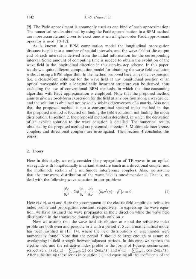
In the first example, we assume Ds ¼ 0:7 mm, Dm ¼ 14 mm, L ¼ 60 mm, ng ¼ 1:8and nc ¼ 1:446. Figure 2(a) and (b) show the calculated distributions of electricfields, respectively, at the middle and the output end of the multimode waveguide. Inthis example, a TE wave (the fundamental mode of the input waveguide) is launchedat the input end of the multimode waveguide. The field distributions here (which isexpressed as "ðx, zÞ ¼

PNn¼0 enðzÞ cos ð2npx=T Þ) were obtained with T ¼ 200 mm and

N ¼ 265 through computation of the vector EðzÞ by using equation (5). The averageof the propagation constants of all guided modes was used for � in equation (5).To compare our method with others, we have also used two commercial softwares tocompute the field distributions for the same case. Figure 3 shows the correspondingelectric field distributions obtained by using Beam-PROP with the approximationof Pade ð4, 4Þ order. Figure 3 (a) and (b) are the results at the middle and the outputend of the multimode waveguide, respectively. It can be seen from figures 2 and 3that for field distributions at two positions (i.e. at the middle and the output end ofthe multimode waveguide), Beam-PROP and the proposed method produce almost

L

sD

Input waveguide

Refractive index gn

Refractive index cn

mD

Z=L Z=0 Multimode waveguide

Figure 1. MMIC slab waveguide under study. Ds and Dm are the widths of the inputwaveguide and multimode waveguide, respectively. The refractive indices of the cores of bothwaveguides are the same (denoted by ng). Both waveguides also have the same refractive index(denoted by nc) for the claddings.

1344 C.-S. Hsiao et al.

|E|

|E|

(a)

(b)

−30 30X (mm)

Figure 2. Distributions of electric fields at (a) the middle and (b) the output end of themultimode waveguide, obtained by using equation (5), for the MMIC structure shownin figure 1. The parameters Ds ¼ 0:7mm, Dm ¼ 14mm, L ¼ 60mm, ng ¼ 1:8, nc ¼ 1:446 areused here.

|E|

|E|

(a)

(b)

−30 30

X (mm)

Figure 3. Distributions of electric fields at (a) the middle and (b) the output end of themultimode waveguide, obtained by using the commercial software Beam-PROP (Pade orderð4, 4Þ). The parameters Ds ¼ 0:7 mm, Dm ¼ 14 mm, L ¼ 60mm, ng ¼ 1:8, nc ¼ 1:446 are usedhere.

A closed-form solution for wave propagation in optical waveguides 1345

identical results (note that the discrepancy between both results is quite negligible).

Another commercial software (BPM-CAD) was also used and the same result wasfound.

Note that the example above refers to a non-weakly guiding waveguide, in whichthe paraxial approximation usually can not apply. Consequently, the second

derivative of the electric field amplitude with respect to distance in the wave equation(i.e. the term d2E=dz2 in equation (2)) cannot be neglected in computing the wave

evolution along the non-weakly guiding waveguide. In the conventional methods,a beam propagation scheme with a wide-angle (especially Pade) approximation is

employed to obtain the wave evolution. As we can see from the previous section,however, the solution method proposed here does not require a beam propagation

scheme, which usually induces a long computational time period as a step-by-stepalgorithm is needed. In the present example, only eigenvalues and eigenvectors ofa small-sized matrix (e.g. a 265� 265 one in the example) need to be found. Note

that a CPU time of less than 7.7 s (in Matlab language) is needed for the proposedmethod (for figure 2), while more than 80 s CPU time is consumed for Beam-PROP

(for figure 3). It is clear that the proposed solution method (cf. equation (5)) is analternative for studying wave field evolution without using a beam propagation

algorithm. Figure 4 shows the corresponding field distributions at the middle andthe output end of the multimode waveguide, obtained by using Beam-PROP with

the second derivative of the electric field amplitude neglected in the wave equation,a condition identical to that in which the term d2E=dz2 in equation (2) is dropped.

A substantial discrepancy between this result and that shown in figure 3 is clear,indicating the necessity for the second derivative term in obtaining an exact solution.

−30 30

(a)

(b)

|E|

|E|

X (mm)

Figure 4. Distributions of electric fields at (a) the middle and (b) the output end of themultimode waveguide, obtained by using the commercial software Beam-PROP (Pade orderð1, 0Þ). The parameters Ds ¼ 0:7 mm, Dm ¼ 14 mm, L ¼ 60mm, ng ¼ 1:8, nc ¼ 1:446 areused here.

1346 C.-S. Hsiao et al.

In many other cases in which the paraxial approximation is not valid, our methodproposed here provides a useful alternative for studying the wave evolution alonga longitudinally invariant waveguide.

In the case that the paraxial approximation is valid, equation (2) reduces to thematrix equation dE=dz ¼ �iB � E=ð2�Þ, the solution of which is given as

EðzÞ ¼XNn¼0

cnEn exp ½�i�nz=ð2�Þ� , ð6Þ

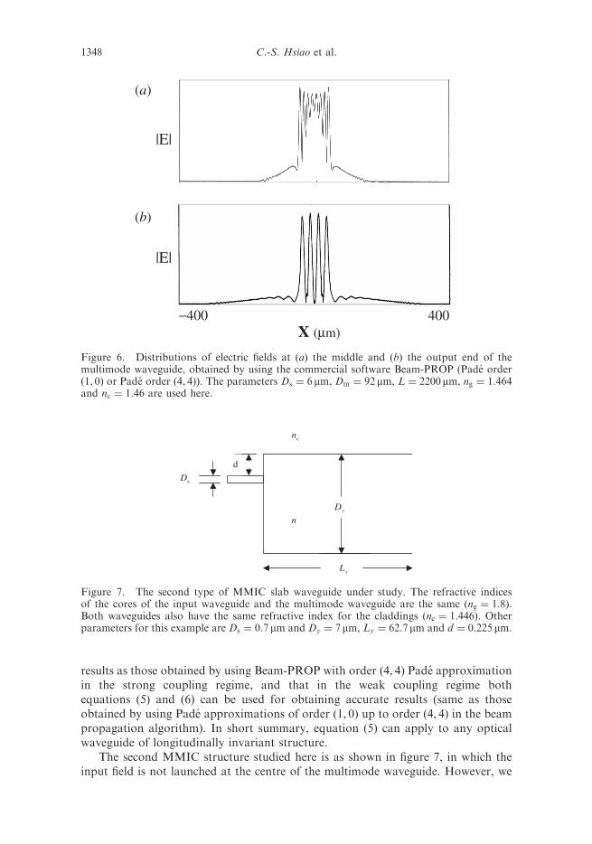
where En and �n (n ¼ 0, 1, 2, . . . ,N) are the eigenvector and eigenvalue of B,respectively; cn (n ¼ 0, 1, 2, . . . ,N) is a constant dependent on the initial condition.The following example for the MMIC structure shown in figure 1 corresponds tothe case of a weakly guiding waveguide: Ds ¼ 6 mm, Dm ¼ 92 mm, L ¼ 2200 mm,ng ¼ 1:464 and nc ¼ 1:46. Because the paraxial approximation is valid in thisexample, the solutions given in equations (5) and (6) are almost identical.Figure 5 (a) and (b) show the calculated electric field distributions, respectively, atthe middle and the output end of the multimode waveguide. These results are in greatagreement with those obtained by using Beam-PROP with Pade approximationsof order ð1, 0Þ up to order ð4, 4Þ. Figure 6 shows the result obtained by using Beam-PROP. Note that we have used T ¼ 850 mm and N ¼ 120 in using equation (5) toobtain accurate results in this example. The CPU time consumed by the proposedmethod is less than 1 s in Matlab language.

We have also investigated the waves in directional couplers made of two slabwaveguides adjacent to each other. It was found that equation (5) produces the same

|E|

−400 400

|E|

(a)

(b)

X (mm)

Figure 5. Distributions of electric fields at (a) the middle and (b) the output end of themultimode waveguide, obtained by using our proposed method. These results can be obtainedby using either equation (5) or equation (6). The parameters Ds ¼ 6mm, Dm ¼ 92 mm,L ¼ 2200 mm, ng ¼ 1:464 and nc ¼ 1:46 are used here.

A closed-form solution for wave propagation in optical waveguides 1347

results as those obtained by using Beam-PROP with order (4, 4) Pade approximationin the strong coupling regime, and that in the weak coupling regime bothequations (5) and (6) can be used for obtaining accurate results (same as thoseobtained by using Pade approximations of order ð1, 0Þ up to order ð4, 4Þ in the beampropagation algorithm). In short summary, equation (5) can apply to any opticalwaveguide of longitudinally invariant structure.

The second MMIC structure studied here is as shown in figure 7, in which theinput field is not launched at the centre of the multimode waveguide. However, we

|E|

|E|

−400 400

(a)

(b)

X (mm)

Figure 6. Distributions of electric fields at (a) the middle and (b) the output end of themultimode waveguide, obtained by using the commercial software Beam-PROP (Pade orderð1, 0Þ or Pade order ð4, 4Þ). The parameters Ds ¼ 6mm, Dm ¼ 92mm, L ¼ 2200mm, ng ¼ 1:464and nc ¼ 1:46 are used here.

yD

yL

n

cn

sD

d

Figure 7. The second type of MMIC slab waveguide under study. The refractive indicesof the cores of the input waveguide and the multimode waveguide are the same (ng ¼ 1:8).Both waveguides also have the same refractive index for the claddings (nc ¼ 1:446). Otherparameters for this example are Ds ¼ 0:7 mm and Dy ¼ 7mm, Ly ¼ 62:7mm and d ¼ 0:225 mm.

1348 C.-S. Hsiao et al.

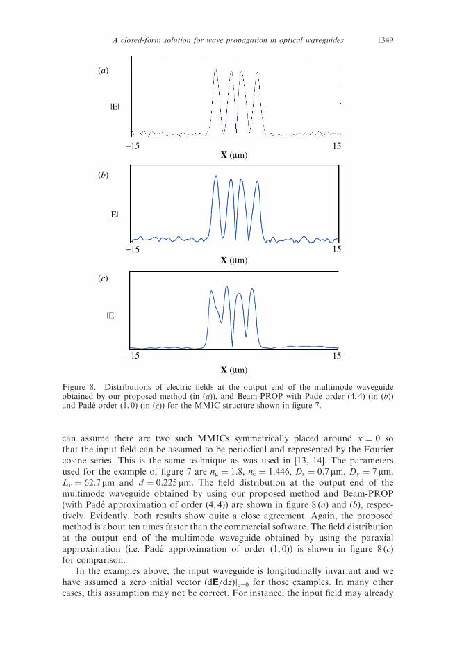
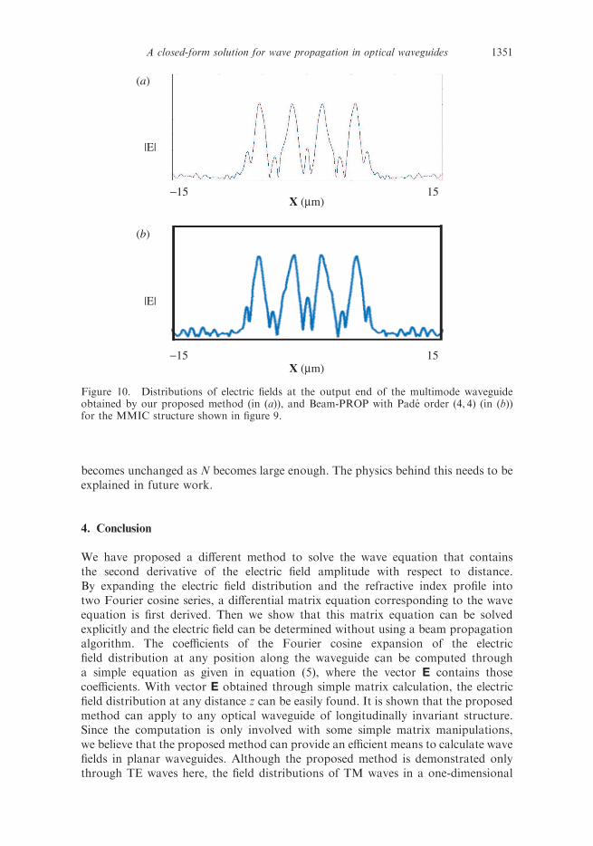
can assume there are two such MMICs symmetrically placed around x ¼ 0 sothat the input field can be assumed to be periodical and represented by the Fouriercosine series. This is the same technique as was used in [13, 14]. The parametersused for the example of figure 7 are ng ¼ 1:8, nc ¼ 1:446, Ds ¼ 0:7 mm, Dy ¼ 7 mm,Ly ¼ 62:7 mm and d ¼ 0:225 mm. The field distribution at the output end of themultimode waveguide obtained by using our proposed method and Beam-PROP(with Pade approximation of order ð4, 4Þ) are shown in figure 8 (a) and (b), respec-tively. Evidently, both results show quite a close agreement. Again, the proposedmethod is about ten times faster than the commercial software. The field distributionat the output end of the multimode waveguide obtained by using the paraxialapproximation (i.e. Pade approximation of order ð1, 0Þ) is shown in figure 8 (c)for comparison.

In the examples above, the input waveguide is longitudinally invariant and wehave assumed a zero initial vector (dE=dzÞjz¼0 for those examples. In many othercases, this assumption may not be correct. For instance, the input field may already

−15 15

15

15

|E|

(a)

|E|

(b)

|E|

(c)

−15

−15

X (mm)

X (mm)

X (mm)

Figure 8. Distributions of electric fields at the output end of the multimode waveguideobtained by our proposed method (in (a)), and Beam-PROP with Pade order (4, 4) (in (b))and Pade order (1, 0) (in (c)) for the MMIC structure shown in figure 7.

A closed-form solution for wave propagation in optical waveguides 1349

be divergent before it enters the multimode waveguide, in which case the initial

vector (dE=dzÞjz¼0 is not a zero one. Here, we use a tapered waveguide as an input

waveguide, as indicated in figure 9, and run the proposed algorithm for this case.

The refractive indices are the same as in the case of figure 7. Other parameters for this

example are Ds ¼ 0:7 mm and Dm ¼ 14 mm, Do ¼ 1 mm, Lt ¼ 2 mm and L ¼ 60 mm.

In calculating the field at the output end of the multimode waveguide, we have used

N ¼ 126 and T ¼ 91 mm. It should be noted that a step-by-step method was used

to treat the wave calculation in the tapered section. In this step-by-step method,

equation (5) was used to compute the wave at each next step; it is a pity that we

cannot yet at this moment avoid the use of the beam propagation algorithm as we

did for the multimode waveguide. However, note that the CPU time consumed by

this beam propagation algorithm with equation (5) was much less than that required

by Beam-PROP. The initial vector dE=dzjz¼0 for the multimode waveguide was

calculated as ½Eð�zÞ � Eð��zÞ�=�z, where the small interval �z was set to be

0.01 mm, and was found not to be a zero vector in this case. Figure 10 (a) and (b)

show the field distribution at the output end of the multimode waveguide obtained

by using equation (5) and Beam-PROP, respectively. We can see quite a good

agreement between the two results. It should be noted that the CPU time spent by

our proposed method for the MMIC (which contains the single-mode waveguide,

the tapered waveguide and the multimode waveguide) is 8 s in contrast to 342 s spent

by the commercial software Beam-PROP. Also note that the CPU time for only the

tapered waveguide is about 6 s by our proposed method (with the beam propagation

algorithm used), while the CPU time consumed by Beam-PROP is about 11 s.

The reason for the long CPU time required by Beam-PROP is that the longitudinal

discretization had to be fine enough to reach substantial accuracy. It can then be

seen that our proposed method is more efficient (in terms of CPU time) than the

commercial software even when both apply a step-by-step computational scheme.

Finally it is noted that there is no particular boundary condition assumed at the

transverse limits, and that the radiated wave outside the waveguide would get more

steady as N increases from 126, i.e. the wave distribution outside the waveguide

Figure 9. The third type of MMIC slab waveguide under study, with a tapered waveguideas the input waveguide. The refractive indices are the same as in the case of figure 7.The parameters for this example are Ds ¼ 0:7 mm and Dm ¼ 14 mm, Do ¼ 1 mm, Lt ¼ 2 mmand L ¼ 60 mm.

1350 C.-S. Hsiao et al.

becomes unchanged as N becomes large enough. The physics behind this needs to beexplained in future work.

4. Conclusion

We have proposed a different method to solve the wave equation that containsthe second derivative of the electric field amplitude with respect to distance.By expanding the electric field distribution and the refractive index profile intotwo Fourier cosine series, a differential matrix equation corresponding to the waveequation is first derived. Then we show that this matrix equation can be solvedexplicitly and the electric field can be determined without using a beam propagationalgorithm. The coefficients of the Fourier cosine expansion of the electricfield distribution at any position along the waveguide can be computed througha simple equation as given in equation (5), where the vector E contains thosecoefficients. With vector E obtained through simple matrix calculation, the electricfield distribution at any distance z can be easily found. It is shown that the proposedmethod can apply to any optical waveguide of longitudinally invariant structure.Since the computation is only involved with some simple matrix manipulations,we believe that the proposed method can provide an efficient means to calculate wavefields in planar waveguides. Although the proposed method is demonstrated onlythrough TE waves here, the field distributions of TM waves in a one-dimensional

−15 15

−15 15

|E|

(a)

|E|

(b)

X (mm)

X (mm)

Figure 10. Distributions of electric fields at the output end of the multimode waveguideobtained by our proposed method (in (a)), and Beam-PROP with Pade order (4, 4) (in (b))for the MMIC structure shown in figure 9.

A closed-form solution for wave propagation in optical waveguides 1351

waveguide problem can be found in the same straightforward manner. This state-ment is obviously true as we notice that a matrix equation in the same form as inequation (2) can be derived for the case of TM waves. To be clear, equation (2)would be solved to produce the field evolution of a TM wave, except that thematrix B defined here should be replaced by another constant matrix(i.e. A�W�W0 � Vð

��WW�WW � �AA�1� �2 � I or A�W�W0 � V0 � �2 � I; see [14]). We

state here that the proposed method could be a basis for extending into waveguideproblems with three-dimensional and/or z-variant structures.

Appendix

Consider the diagonization of the matrix B as given by , ¼ Y�1BY, where thematrices Y and , are defined, respectively as

Y ¼ ½P0,P1,P2, . . . ,PN � ðA1Þ

and

, ¼

�0�1

�2

0

0�

�

�N

2666664

3777775

ðA2Þ

with Pi and �i being, respectively, the eigenvector and the corresponding eigenvalueof B (i ¼ 0, 1, 2, . . . ,N). By defining E ¼ Y � F, equation (2) can be transformed intoa matrix equation such as

d2F

dz2� 2i�

dF

dzþ , � F ¼ 0: ðA3Þ

Since , is diagonal, equation (A 3) corresponds simply to a set of second-orderordinary differential equations:

d2fi

dz2� 2i�

dfi

dzþ �i fi ¼ 0, ðA4Þ

where fi’s (i ¼ 0, 1, 2, . . . ,N) are elements of F, as given by F ¼ ½ f0, f1, f2, . . . , fN �t

with ‘t’ representing transpose. The general solution of equation (A 4) for each i isci1 exp ½ði�þ ð��2 � �iÞ

1=2Þz� þ ci2 exp ½ði�� ð��2 � �iÞ

1=2Þz�, where both ci1 and ci2

are constants. Now write the relation E ¼ Y � F in the following form

e0e1e2�

�

�

�

eN

266666666664

377777777775

¼

p00 p10 p20 � � � � pN0

p01 p11 p21 � � � � pN1

p02 p12 p22 � � � � p22� � � � � � � �

� � � � � � � �

� � � � � � � �

� � � � � � � �

p0N p1N p2N � � � � pNN

266666666664

377777777775

�

f0f1f2�

�

�

�

fN

266666666664

377777777775

: ðA5Þ

1352 C.-S. Hsiao et al.

Here we have defined the eigenvector Pi as ½pi0, pi1, pi2, . . . , piN �t. Substituting the

general solution of each fi in equation (A 5), we then find that the vector E can bewritten in the form

E ¼XNi¼0

Pifui exp ½ði�þ ð��2 � �iÞ1=2

Þz� þ bi exp ½ði�� ð��2 � �iÞ1=2

Þz�g , ðA6Þ

where ui and bi (i ¼ 0, 1, 2, . . . ,N) are constants.

References

[1] Y. Chung and N. Dagli, IEEE J. Quantum Electron. QE-26 1335 (1990).[2] H.J.W.M. Hoekstra, G.J.M. Krijnen and P.V. Lambeck, IEEE J. Lightwave Technol.

10 1352 (1992).[3] Y. Chung and N. Dagli. Paper presented at Technical Digest IEEE AP-S International

Symposium 1992, Vol. 1 (IEEE Press, Piscataway, 1992), pp. 248–251.[4] J. Yaamaaucchi, J. Shibayama and H. Nakano, Photon. Technol. Lett. 7 661 (1995).[5] O.C. Zienkiewitz, The Finite Element Method, 3rd edition (McGraw-Hill, New York,

1973).[6] B.M.A. Rahman and J.B. Davis, IEEE J. Lightwave Technol. 2 682 (1984).[7] K. Hayata, M. Koshiba, M. Egushi, et al., Electron. Lett. 22 295 (1986).[8] M. Koshiba, H. Saitoh, M. Eguchi, et al., IEE Proc. J. 139 166 (1992).[9] Y. Chung and N. Dagli, IEEE Photon. Technol. Lett. 6 540 (1994).[10] G.R. Hadley, Opt. Lett. 17 1426 (1992).[11] G.R. Hadley, Opt. Lett. 17 1743 (1992).[12] I. Ilic, R. Scarmozzino and R.M. Osgood Jr, J. Lightwave Technol. 14 2813 (1996).[13] L. Wang and N. Huang, IEEE J. Quantum Electron. 35 1351 (1999).[14] L. Wang and C.S. Hsiao, IEEE J. Quantum Electron. 37 1654 (2001).

A closed-form solution for wave propagation in optical waveguides 1353