Clim. Past, 8, 803–814, 2012www.clim-past.net/8/803/2012/doi:10.5194/cp-8-803-2012© Author(s) 2012. CC Attribution 3.0 License.

Climateof the Past

A climate model intercomparison for the Antarctic region:present and past

M. N. A. Maris, B. de Boer, and J. Oerlemans

Institute for Marine and Atmospheric research Utrecht, Utrecht University, P.O. Box 80005,3508 TA Utrecht, The Netherlands

Correspondence to:M. N. A. Maris (m.n.a.maris@gmail.com)

Received: 7 October 2011 – Published in Clim. Past Discuss.: 24 October 2011Revised: 3 April 2012 – Accepted: 4 April 2012 – Published: 18 April 2012

Abstract. Eighteen General Circulation Models (GCMs)are compared to reference data for the present, the Mid-Holocene (MH) and the Last Glacial Maximum (LGM) forthe Antarctic region. The climatology produced by a regionalclimate model is taken as a reference climate for the present.GCM results for the past are compared to ice-core data. Thegoal of this study is to find the best GCM that can be used todrive an ice sheet model that simulates the evolution of theAntarctic Ice Sheet. Because temperature and precipitationare the most important climate variables when modelling theevolution of an ice sheet, these two variables are consideredin this paper. This is done by ranking the models accordingto how well their output corresponds with the references. Ingeneral, present-day temperature is simulated well, but pre-cipitation is overestimated compared to the reference data.Another finding is that model biases play an important role insimulating the past, as they are often larger than the change intemperature or precipitation between the past and the present.Considering the results for the present-day as well as for theMH and the LGM, the best performing models are HadCM3and MIROC 3.2.2.

1 Introduction

Variations in ice volume of the Antarctic Ice Sheet (AIS)have a large impact on sea level and ocean circulation. Sincethe Last Glacial Maximum (LGM), at approximately 21 ka,the AIS has undergone many changes (e.g.Huybrechts,2002; Bentley, 1999). This is especially true for the WestAntarctic Ice Sheet, which is potentially unstable (see for ex-ample,Hughes, 1975; Thomas, 1979; Bamber et al., 2009).

To study variations in the AIS with a dynamical ice-sheetmodel, realistic (near-surface) air temperature and precipita-tion are needed as input. These variables may be given bya General Circulation Model (GCM) or a Regional ClimateModel (RCM), which in its turn may be driven by a GCMat its lateral boundaries. Therefore it is important to knowwhich GCMs perform well in the Antarctic region.

It is generally accepted that a model performs well whenit is close to the ensemble mean, as was done byZweck andHuybrechts(2005). However, the best GCM for a specificstudy or use might not be the one closest to the ensemblemean. For instance, when using a GCM to drive an RCM,it is important that the GCM produces realistic output closeto the boundaries of the RCM, whereas certain regional bi-ases in the GCM may play a bigger role when studying apart of the AIS. In the literature, different criteria have beendescribed for a GCM to perform “well”, such as high reso-lution (Ren et al., 2011) and low bias (Murphy et al., 2002).However, these studies focus on either only one model or onecriterion, instead of intercomparing a larger set of GCMs.

Comparisons of larger sets of GCMs have been donethrough the Paleoclimate Modelling Intercomparison ProjectPhase II (PMIP2,Braconnot et al., 2007), which has a largedatabase with output from GCMs for the present, the Mid-Holocene (MH) and the LGM. Intercomparison studies ofthe models in this database have been done by, amongst oth-ers,Braconnot et al.(2007), Yanase and Abe-Ouchi(2007),Brewer et al.(2007) and Masson-Delmotte et al.(2006).Only the study ofMasson-Delmotte et al.(2006) focuses onthe polar regions (and therefore Antarctica). They concludethat the PMIP2 models’ simulations agree reasonably wellwith ice-core signals for both the MH and the LGM, although

Published by Copernicus Publications on behalf of the European Geosciences Union.

804 M. N. A. Maris et al.: An Antarctic climate model study

there are uncertainties in the models’ ice-sheet topography,which is based on ICE-5G (Peltier, 2004). However, theirstudy focuses on the ensemble mean of all the models underconsideration and less on the differences between models.

In order to decide which GCMs perform best in theAntarctic region, we compare the individual output of themodels to ice-core reconstructions for the MH and LGM.Furthermore, as ice-core data have large uncertainty and donot cover the entire Antarctic region, we compare present-day GCM data to a reference state from RACMO2/ANT(Lenaerts et al., 2012a). RACMO2/ANT (simply “RACMO”hereafter) is a regional climate model, which has been devel-oped especially for polar regions and has been thoroughlyvalidated (e.g.van de Berg et al., 2005; Lenaerts et al.,2012b).

2 Method

Eighteen models from the PMIP2 database, see Table1, arecompared with reference data from RACMO for the present-day climate and with ice-core climate reconstructions forthe past. The GCM data used for this study originate fromcoupled ocean-atmosphere models. Some of the models areclosely related to others: UBRIS-HadCM3 and HadCM3 aremuch alike; CSIRO-1.1 is the same as CSIRO-1.0, but witha doubled oceanic resolution; MRI-fa uses flux adjustmentsfor heat and water fluxes and wind stress, whereas MRI-nfadoes not; and MIROC 3.2.2 is the same as MIROC 3.2, butan error in the land surface scheme of MIROC 3.2 has beencorrected in MIROC 3.2.2, affecting the wind stress calcula-tion over ice sheets and resulting in somewhat lower temper-atures. Nonetheless, MIROC 3.2 has been included in thisstudy because there are additional (Mid-Holocene) simula-tions available for this model.

The present-day reference state originates from RACMO,at a horizontal resolution of 27 km. RACMO is forced at itslateral boundaries by ERA-Interim reanalysis data for 20 yr(1989–2009). RACMO has been chosen because it pro-vides data at a high resolution. Furthermore, temperatureand precipitation have a smaller bias than reanalysis prod-ucts such as ERA-40 or ERA-Interim (van de Berg et al.,2006, 2007; van de Berg, 2008; Ettema et al., 2010; Lenaertset al., 2012b). The uncertainty in RACMO precipitation isabout 10 % (Lenaerts et al., 2012b). The uncertainty in 2mair temperature is more difficult to determine, a plot of thedifference between yearly average RACMO skin temperatureand observed temperatures at 10 m depth is shown in Fig.1.The difference between modelled and observed temperaturesis small, except for parts of the Western Antarctic Ice Sheet.

The RACMO-domain runs from 90◦ South to approxi-mately 47◦ South. We compared 2 m air temperature andannual mean precipitation from the GCMs with RACMO-data. To this purpose all GCM data are interpolated on theRACMO grid. No lapse rate correction has been applied

Fig. 1. A map of the Antarctic continent showing the yearly aver-age temperature difference between RACMO and observations, atlocations were observations have been made.

to the GCM data to compensate for the mismatches in sur-face height between the GCMs and RACMO. This is becausewhen the same analysis as the one described in this paperwas performed on the GCM data with a lapse rate correc-tion of −11.6 K km−1 (Masson-Delmotte et al., 2011), thisdid not change the results much and introduced uncertaintiesthat were not in the GCM output initially.

The data are compared regarding bias, root mean squaredeviation (rmsd), and correlation coefficient (ρ):

bias=

∑Ni=1xGi

− xRi

N, (1)

rmsd=

√∑Ni=1(xGi

− xRi)2

N, and (2)

ρ =

∑Ni=1(xGi

− xG) · (xRi− xR)√∑N

i=1(xGi− xG)2 ·

∑Ni=1(xRi

− xR)2, (3)

in which the subscriptsG and R stand for GCM andRACMO, respectively, andx indicates the average of thevariablex over all grid pointsi.

The correlation coefficient indicates how well temperatureand precipitation patterns are simulated by a model, whereasthe bias (mean deviation of the model from the reference)and the rmsd (a measure for the absolute deviation of themodel from the reference) quantify how much the model out-put deviates from the reference state as a whole. A distinc-tion is made between results over the ice sheet, including iceshelves (Fig.3) and results over the ocean (Fig.4). The bias,

Clim. Past, 8, 803–814, 2012 www.clim-past.net/8/803/2012/

M. N. A. Maris et al.: An Antarctic climate model study 805

Table 1. The models evaluated in this study, with the abbreviations used in this paper, their horizontal resolution and the length of the periodused to determine the climatological mean. Crosses indicate whether the model provided output for 6 ka and/or 21 ka.

Model name in PMIP2Abbreviation

Resolution Averaging6 ka 21 ka

database lon× lat time (yr)

CCSM CCSM 2.81◦ × 2.81◦ 100 X XCNRM-CM33 CNRM 2.81◦ × 2.81◦ 300 XCSIRO-Mk3L-1.0 CSIRO-1.0 5.63◦ × 3.22◦ 100 XCSIRO-Mk3L-1.1 CSIRO-1.1 5.63◦ × 3.22◦ 50 XECBILTCLIO Ecbiltclio 5.63◦ × 5.63◦ 50 XECBILTCLIOVE-CODE Ecbiltcliove 5.63◦ × 5.63◦ 100 XECHAM5-MPIOM1 ECHAM5 3.75◦ × 3.75◦ 50 XECHAM53-MPIOM127-LPJ ECHAM53 3.75◦ × 3.75◦ 100 X XFGOALS-1.0g FGOALS 2.81◦ × 3◦ 100 X XFOAM FOAM 7.5◦ × 4.5◦ 100 XGISSmodelE GISS 5◦ × 3.92◦ 50 XHadCM3M2 HadCM3 3.75◦ × 2.5◦ 100 XIPSL-CM4-V1-MR IPSL 3.75◦ × 2.5◦ 100 X XMIROC 3.2 MIROC 3.2 2.81◦ × 2.81◦ 50 X XMIROC 3.2.2 MIROC 3.2.2 2.81◦ × 2.81◦ 100 XMRI-CGCM2.3.4fa MRI-fa 2.81◦ × 2.81◦ 100 XMRI-CGCM2.3.4nfa MRI-nfa 2.81◦ × 2.81◦ 100 XUBRIS-HadCM3M2 UBRIS 3.75◦ × 2.5◦ 100 X

rmsd and correlation coefficient have been chosen becausetogether they give a good overview of whether the GCMs canreproduce the correct patterns and realistic absolute values oftemperature and precipitation.

In the second part of this study, GCM output for the MH(6 ka) and the LGM (21 ka) is compared to the present. Dif-ferences between the past and the present are evaluated, us-ing reconstructions from ice cores (see Fig.2 for their loca-tions). Temperature data are available from six ice cores forboth the MH and the LGM:

– EPICA Dome C (EDC), a deuterium excess based tem-perature reconstruction byJouzel and Masson-Delmotte(2007).

– EPICA Dronning Maud Land (EDML), a deuterium andδ18O based temperature reconstruction. The1T for theMH was read from Fig. 7b byStenni et al.(2010), the1T for the LGM is mentioned in their paper as well.

– Dome Fuji (Fuji), a deuterium andδ18O based temper-ature reconstruction byKawamura et al.(2007).

– Law Dome (LD), aδ18O reconstruction is given inFig. 5 in van Ommen et al.(2004). Past temperaturesmay be calculated from this graph by using a conver-sion of 0.44 ‰◦C−1. Details were communicated invanOmmen(2011).

– Vostok, a deuterium temperature reconstruction byPetitet al.(1999).

Precipitation records are scarce as they are more difficult toderive from ice cores. The precipitation reconstructions usedin this study are:

– Law Dome, the accumulation rate is determined from aflow model together with age-ties invan Ommen et al.(2004), the reconstructions are given in Table 2 of theirpaper.

– Talos Dome, aδ18O based precipitation reconstructionis given in Fig. 7 inBuiron et al. (2011) in cm iceequivalent per year. To get the precipitation change inmm water equivalent per year, the number is multipliedby 9.2.

– Vostok, a reconstruction based on10Be, given in Fig. 7in Steig et al.(2000).

The model output is compared to ice-core data with re-spect to the temperature difference between the past and thepresent, the precipitation difference between the past and thepresent and the ratio of past to present precipitation, whereboth past and present-day data originate from the GCMs.The precipitation ratio is given because some models givea correct change in precipitation, but overestimate the actualamount both in the past and for the present-day. In this casethe modelled ratio will be larger than the ratio deduced fromthe corresponding ice core. The comparison is carried out byinterpolating the data from the four grid points of the GCMclosest to the location of the ice core.

The goal of this study is to find the best models regard-ing simulations of temperature and precipitation. To do this

www.clim-past.net/8/803/2012/ Clim. Past, 8, 803–814, 2012

806 M. N. A. Maris et al.: An Antarctic climate model study

Table 2. Reconstructed and modelled temperature differences (inKelvin) between the MH and the present at five ice-core locations.Modelled temperature differences are calculated by interpolatingthe four closest model data points.

EDC EDML Fuji LD Vostok

Ice core −0.4 0.5 −0.4 1.3 0.4

CCSM 0.1 0.0 0.1 0.0 0.3CSIRO-1.0 0.4 0.3 0.4 0.3 0.4CSIRO-1.1 0.2 0.9 0.0 0.4 0.4Ecbiltcliove 0.3 0.3 0.1 0.4 0.1ECHAM5 0.2 0.2 0.6 0.4 0.4ECHAM53 0.4 0.0 0.4 0.3 0.5FGOALS 0.1 0.3 0.5 0.2 0.2FOAM 0.5 0.7 0.6 0.9 0.7GISS −0.3 −0.6 −0.2 −0.1 −0.1IPSL 0.6 0.6 0.5 0.4 0.4MIROC 3.2 0.2 0.1 0.3 0.4 0.4MRI-fa 0.2 0.1 0.4 0.9 0.3MRI-nfa −0.4 −0.4 −0.5 −0.9 −0.2UBRIS 0.7 0.8 0.8 0.1 0.7

a simple ranking system is introduced: the best model for acertain variable, e.g. temperature bias of the present-day out-put, gets 10 points, the next gets 9 points, etc. For every pe-riod (i.e. present-day, MH and LGM) these points are addedup per model resulting in a ranking of the models for eachof the periods. When multiple models have the same amountof points, the spread is taken into account. That is to say, amodel is judged to be better when an intermediate numberof points is scored for all the variables than the maximumnumber of points for only half of the variables.

3 Present-day results

Figure 3a shows the bias (in red) and the rmsd (in blue)for the present-day temperature comparison between thePMIP2-models and RACMO over the ice sheet and iceshelves. The biases range from−3.8 K (MRI-nfa) to +4.8 K(Ecbiltclio) and the rmsd values go up to 10.3 K (Ecbilt-clio) for the temperature. Temperature correlation coeffi-cients (shown in Fig.3c in red for the temperature) are closeto 1, ranging from 0.89 to 0.97, for all models except forEcbiltclio and Ecbiltcliove-code.

Precipitation bias and rmsd are presented in Fig.3b.The highest bias is +349 mm yr−1 for FGOALS, which alsoshows the highest rmsd value of 463 mm yr−1. Precipitationcorrelation coefficients show a larger spread than for tem-perature, from 0.51 to 0.82. The largest bias and rmsd arefound for the precipitation output of FGOALS and the tem-perature output of Ecbiltclio, which might be due to the lowresolution of the model. As mentioned before, the modelMIROC 3.2.2 should give lower temperatures (and therefore

Fig. 2. A map showing the Antarctic continent with three iceshelves highlighted and the locations of the six ice cores used inthis study.

a smaller temperature bias) than MIROC 3.2 due to a cor-rected error in MIROC 3.2.2, which is indeed the case.

In Fig. 4 the same variables are presented as in Fig.3, butfor a domain that only incorporates the ocean grid points ofRACMO. Again, the temperature correlation coefficients aremostly close to 1, ranging from 0.86 to 0.96. Precipitationcorrelation coefficients are slightly larger here than over theice sheet (from 0.60 to 0.87). Rmsd values are smaller, whilebias values are generally somewhat larger, i.e. more negative,over the ocean.

The four models that simulate the present-day climate bestare UBRIS, HadCM3, ECHAM5 and IPSL for temperatureand UBRIS, HadCM3, ECHAM5, and MIROC 3.2 for pre-cipitation. This is based on the ranking method, appliedon the combination of the results over the ice sheet and theocean. The difference fields between these best models andRACMO are shown in Fig.5 for temperature and Fig.6 forprecipitation.

A notable feature in Fig.5 is that the modelled tempera-tures over the Ross ice shelf (see Fig.2) are too high, whichis the case for almost all models. At the locations of theseice shelves, land is modelled by the GCMs, which is onlypartly covered with ice. In contrast, over the Amery IceShelf region the models simulate too low temperatures. Thisis something to take into account when deciding on whichmodel to use. For example, when focussing on West Antarc-tica, HadCM3 shows less (negative) bias there than the othermodels and might be a better choice because RACMO showsa negative bias here as well when compared to observations.The modelled temperatures are closer to the reference dataover the ocean, at the edges of the domain.

Clim. Past, 8, 803–814, 2012 www.clim-past.net/8/803/2012/

M. N. A. Maris et al.: An Antarctic climate model study 807

Fig. 3. The bias (red) and rmsd (blue) for temperature(a) and pre-cipitation(b), and spatial correlation coefficients(c) for temperature(red) and precipitation (blue) for all PMIP2 models, as compared tothe RACMO reference state. These results apply to the ice sheet,for the present-day climate.

Precipitation is generally overestimated inland. It is un-derestimated close to the coasts and strongly underestimatedat the western side of the Antarctic Peninsula by all models.This is probably due to the fact that the steep orography ofthe Peninsula is not well represented in the GCMs. Conse-quently, the orographically enhanced precipitation is under-estimated (Rojas et al., 2009).

4 Mid-Holocene results

Mid-Holocene temperature output from the models is com-pared to reconstructions from five ice cores in Table2.The uncertainty ranges of these reconstructions are probablylarger than the small differences in temperature between theMH and the present. The models also simulate small temper-ature differences between the MH and the present. However,the models do not capture the change in sign of the temper-ature differences between different locations, i.e. EDC and

Fig. 4. The bias (red) and rmsd (blue) for temperature(a) and pre-cipitation(b), and spatial correlation coefficients(c) for temperature(red) and precipitation (blue) for all PMIP2 models, as compared tothe RACMO reference state. These results apply to the ocean, forthe present-day climate.

Fuji were colder in the MH than in the present and the tem-perature difference was largest at Law Dome.

For temperature, the best models according to the rank-ing method are CSIRO-1.1 and IPSL. The spatial distribu-tion of the temperature difference between the MH and thepresent (both MH and present temperature values are fromGCM output) are shown in Fig.7. Temperature differencesare mainly positive, but small, except over the western SouthPacific Ocean in Fig.7b (IPSL). Although this difference be-tween the models may not be of much importance when us-ing GCM output in an ice-sheet model, it is important whenonly using the output to provide boundary conditions for anRCM. The negative temperature differences over the westernocean in IPSL cannot be affirmed nor negated by ice-corereconstructions. It may therefore be concluded that the com-parison of model output with ice-core reconstructions givesan indication of which models are better than others, but it isnot conclusive. This is even more true for precipitation, as isargued below.

www.clim-past.net/8/803/2012/ Clim. Past, 8, 803–814, 2012

808 M. N. A. Maris et al.: An Antarctic climate model study

Fig. 5. Present-day temperature difference fields of(a) UBRIS, (b) HadCM3,(c) ECHAM5 and(d) IPSL with RACMO, interpolated on theRACMO grid.

In Table3 precipitation data are shown for three ice-corelocations. The Law Dome data are not very accurate asonly the average accumulation between age ties (2545 and6778 yr ago) is known (van Ommen et al., 2004). At theTalos Dome location, the difference in precipitation between6 ka and the present is captured by most GCMs, but the ratiosare too high. This means that, at this location, the absoluteamounts of precipitation are overestimated by the models inboth present and past. This can be seen in Fig.6 as well. Pre-cipitation at the Vostok location is simulated quite accuratelyby most of the GCMs.

CCSM and Ecbiltcliove precipitation differences betweenthe MH and the present are shown in Fig.8, as these are thebest models according to the ranking method. It is clearlyvisible that the patterns are not the same for these two mod-els. The question remains which model is the better one.The differences between 6 ka and the present are small, andthe biases are of the same order of magnitude. This makesit hard to distinguish between the GCMs in terms of perfor-mance for the MH.

To investigate the influence of biases in simulating thepresent climate on model performance when simulating thepast, a signal-to-noise ratio has been calculated for both tem-perature and precipitation. The signal is the difference, intemperature or precipitation, between 6 ka and the present.The noise is the present-day bias of a model, as shown inFigs.3 and4. For precipitation the average signal-to-noiseratio of all GCMs is 0.09, which is very low. This meansthat the signal is practically indistinguishable from the data.The mean signal-to-noise ratio for temperature is 0.21. Com-bining this with the presumably large uncertainties in theice-core reconstructions, compared to the signal, judgementsabout which models achieve the best results for the MH can-not be accurately made.

5 LGM results

In Table 4 modelled temperature differences between theLGM and the present are compared to data from five icecores. At Law Dome the temperature difference is thelargest, which is not captured by any of the GCMs, except for

Clim. Past, 8, 803–814, 2012 www.clim-past.net/8/803/2012/

M. N. A. Maris et al.: An Antarctic climate model study 809

Fig. 6. Relative present-day precipitation difference fields of(a) UBRIS, (b) HadCM3,(c) ECHAM5 and(d) MIROC 3.2 with RACMO (asa percentage of RACMO precipitation).

Fig. 7. Temperature difference fields between 6 ka and the present for(a) CSIRO-1.1 and(b) IPSL.

www.clim-past.net/8/803/2012/ Clim. Past, 8, 803–814, 2012

810 M. N. A. Maris et al.: An Antarctic climate model study

Fig. 8. Relative precipitation difference fields (as a percentage of the present-day precipitation) between 6 ka and the present for(a) CCSMand(b) Ecbiltcliove.

Table 3. Reconstructed and modelled precipitation differences (in mm yr−1) between 6 ka and the present, and ratios of the 6 ka to thepresent precipitation at three ice-core locations.

Law Dome Talos Vostok

Difference Ratio Difference Ratio Difference Ratio

Ice core 0 1.0 −10 0.9 0.5 1.0

CCSM −3 1.0 −4 1.0 0.1 1.0CSIRO-1.0 9 1.0 11 1.1 0.3 1.0CSIRO-1.1 14 1.0 14 1.1 1.0 1.1Ecbiltcliove −10 1.0 −15 1.0 0.7 1.0ECHAM5 34 1.1 −4 1.0 −0.2 1.0ECHAM53 18 1.0 5 1.0 0.1 1.0FGOALS 10 1.0 29 1.1 0.6 1.0FOAM 22 1.1 1 1.0 0.6 1.0GISS −15 1.0 39 1.1 −0.9 1.0IPSL 44 1.1 14 1.1 1.0 1.1MIROC 3.2 52 1.1 8 1.0 −0.1 1.0MRI-fa 17 1.0 −6 1.0 −0.6 1.0MRI-nfa −21 1.0 −8 1.0 4.1 1.0UBRIS 25 1.1 6 1.0 −0.7 1.0

Ecbiltclio. However, Ecbiltclio generally simulates too smalltemperature differences between the LGM and the present.This holds for CNRM as well, whereas FGOALS overesti-mates the temperature differences at four of the five loca-tions. According to the ranking method, MIROC 3.2.2 andCCSM are the best models. Output from these models isshown in Fig.9.

MIROC 3.2.2 simulates smaller temperature differencesthan CCSM, which is also visible in Table4. Both modelsshow larger temperature differences over West Antarctica,which is the case for almost all models with LGM output.This is probably due to the change in topography, as the dif-ference between the LGM and the present in ice thickness

of the West Antarctic Ice Sheet is larger than the differenceof the East Antarctic Ice Sheet. This agreement betweenthe models regarding the temperature pattern over the icesheet gives some confidence when using either one as in-put in an ice-sheet model. However, when using the data todrive an RCM, the boundaries become important, as has beennoted before, and the differences between MIROC 3.2.2 andCCSM might play a bigger role.

Modelled precipitation differences between the LGM andthe present are compared to reconstructions for Law Dome,Talos Dome and Vostok data in Table5. For Law Domethe LGM-precipitation was less than 10 % of the present-dayvalue. Law Dome is located near the coast, where it receives

Clim. Past, 8, 803–814, 2012 www.clim-past.net/8/803/2012/

M. N. A. Maris et al.: An Antarctic climate model study 811

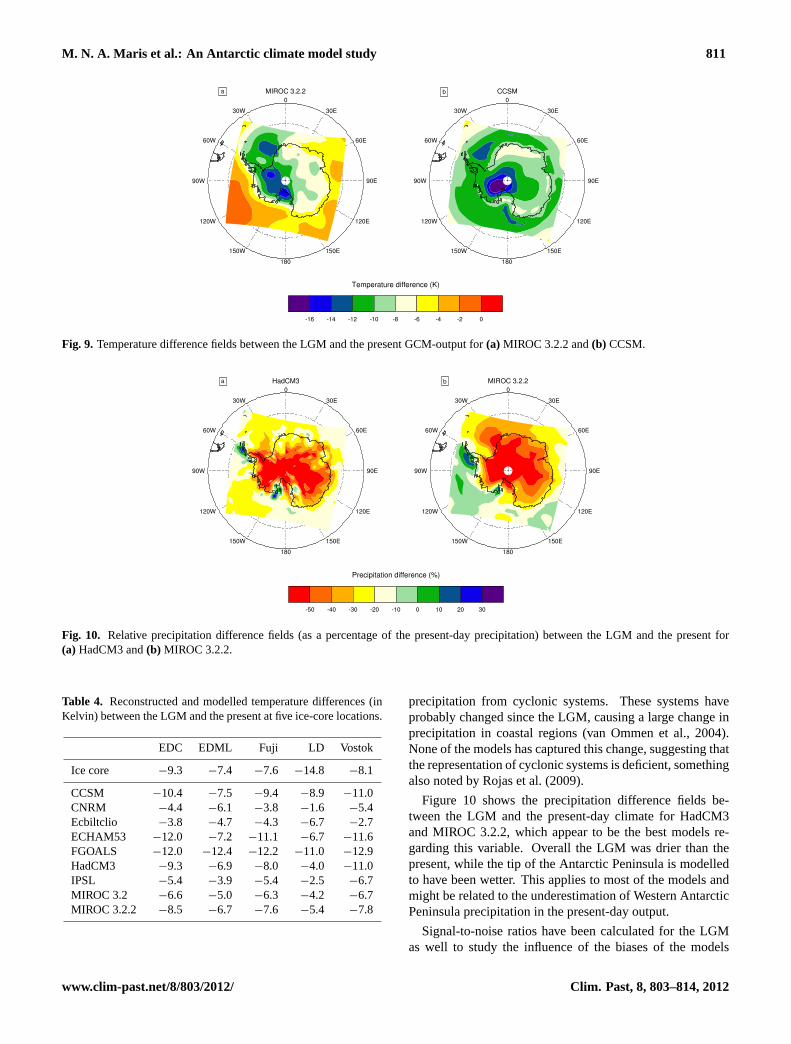
Fig. 9. Temperature difference fields between the LGM and the present GCM-output for(a) MIROC 3.2.2 and(b) CCSM.

Fig. 10. Relative precipitation difference fields (as a percentage of the present-day precipitation) between the LGM and the present for(a) HadCM3 and(b) MIROC 3.2.2.

Table 4. Reconstructed and modelled temperature differences (inKelvin) between the LGM and the present at five ice-core locations.

EDC EDML Fuji LD Vostok

Ice core −9.3 −7.4 −7.6 −14.8 −8.1

CCSM −10.4 −7.5 −9.4 −8.9 −11.0CNRM −4.4 −6.1 −3.8 −1.6 −5.4Ecbiltclio −3.8 −4.7 −4.3 −6.7 −2.7ECHAM53 −12.0 −7.2 −11.1 −6.7 −11.6FGOALS −12.0 −12.4 −12.2 −11.0 −12.9HadCM3 −9.3 −6.9 −8.0 −4.0 −11.0IPSL −5.4 −3.9 −5.4 −2.5 −6.7MIROC 3.2 −6.6 −5.0 −6.3 −4.2 −6.7MIROC 3.2.2 −8.5 −6.7 −7.6 −5.4 −7.8

precipitation from cyclonic systems. These systems haveprobably changed since the LGM, causing a large change inprecipitation in coastal regions (van Ommen et al., 2004).None of the models has captured this change, suggesting thatthe representation of cyclonic systems is deficient, somethingalso noted byRojas et al.(2009).

Figure 10 shows the precipitation difference fields be-tween the LGM and the present-day climate for HadCM3and MIROC 3.2.2, which appear to be the best models re-garding this variable. Overall the LGM was drier than thepresent, while the tip of the Antarctic Peninsula is modelledto have been wetter. This applies to most of the models andmight be related to the underestimation of Western AntarcticPeninsula precipitation in the present-day output.

Signal-to-noise ratios have been calculated for the LGMas well to study the influence of the biases of the models

www.clim-past.net/8/803/2012/ Clim. Past, 8, 803–814, 2012

812 M. N. A. Maris et al.: An Antarctic climate model study

Table 5. Reconstructed and modelled precipitation differences (in mm yr−1) between the LGM and the present, and the ratios of the LGMto the present precipitation at three ice-core locations.

Law Dome Talos Vostok

Difference Ratio Difference Ratio Difference Ratio

Ice core −584 0.1 −39 0.4 −8 0.6

CCSM −118 0.6 −119 0.5 −20 0.3CNRM −99 0.8 22 1.1 −9 0.7Ecbiltclio 6 1.0 −186 0.6 −103 0.5ECHAM53 −148 0.7 −104 0.6 −23 0.3FGOALS −919 0.4 −226 0.6 −43 0.4HadCM3 −165 0.7 −36 0.7 −17 0.3IPSL 18 1.0 −8 1.0 −9 0.5MIROC 3.2 −106 0.8 −37 0.9 −14 0.5MIROC 3.2.2 −137 0.7 −77 0.7 −13 0.5

on the simulation of precipitation and temperature patternsat 21 ka. The average signal-to-noise ratio for temperatureis 3.8, which is significantly larger than 1. Overall this ratiomeans that the signal of temperature change from the LGMto the present is discernible when studying the model output.For precipitation the mean signal-to-noise ratio is 1.4, whichis lower than the temperature signal-to-noise ratio. The pre-cipitation signal-to-noise ratios are lower than the temper-ature signal-to-noise ratios for both the MH and the LGM.The reason for this is probably that precipitation is harder tomodel correctly than temperature, and therefore the biasesare relatively larger. Although the signal-to-noise ratios forthe LGM are higher than for the MH, it is still essential to beaware of the (present-day) bias of a model to correctly assessits output for the LGM.

6 Conclusions

In this paper we compared present-day output from GCMsto a reference state from the regional climate modelRACMO2/ANT for the Antarctic region. We found that air-temperature patterns are generally well simulated, as the cor-relation coefficients between the GCM output and the refer-ence data are close to 1. Temperature is generally more cor-rectly simulated over the ocean than over the ice sheet. Thetemperature over the ice shelves is too high in most of themodels, which is probably due to the fact that there is land atthe locations of the ice shelves in the GCMs, which is onlypartly covered with ice.

Precipitation patterns are also well simulated in general,but the amount of precipitation is often underestimated overthe ocean. In addition, a strong negative bias is observedover the western coast of the Antarctic Peninsula. The GCMsprobably do not resolve the circulation pattern and the orog-raphy well enough to simulate the additional precipitation inthis region (Rojas et al., 2009). Considering temperature and

precipitation results for the present-day, the top five mod-els are HadCM3, UBRIS, which is a HadCM3-based model,ECHAM5, MIROC 3.2, and IPSL.

The differences in temperature and precipitation betweenthe Mid-Holocene and the present are small in ice-core re-constructions and in the output from the GCMs. Generally,both temperature and precipitation are higher during the MHthan in the present climate. The differences between the MHand the present are small, and the biases of the GCMs areof the same order of magnitude or even larger. Therefore,it is hard to judge individual model performances. For theMH, the signal-to-noise ratios are 0.21 for temperature and0.09 for precipitation. These low signal-to-noise ratios indi-cate that to find a model that performs well when modellingthe past, it is important to take its present-day performanceinto account. Furthermore, the uncertainties in ice-core dataare presumably as large as the signal as well, making it evenharder to judge the performance of the models. Based on thecomparison between the output of the GCMs and the ice-corereconstructions for the MH, the five best models are Ecbilt-cliove, CCSM, MRI-fa, MRI-nfa and CSIRO-1.0. However,in the final judgement of which GCMs perform best over-all, the MH will not be taken into consideration as the bi-ases in the models are too large to make the intercomparisontrustworthy.

In the LGM, temperatures were lower and there was lessprecipitation than in the present-day climate, according toboth ice-core reconstructions and GCM output. Also, thetemperature difference between the LGM and the presentis modelled to be larger over the West Antarctic Ice Sheetthan over the East Antarctic Ice Sheet by most GCMs. Theprecipitation differences between the LGM and the presentover the Antarctic Peninsula are generally modelled to besmaller than elsewhere, or even positive (wetter at the LGMthan in the present). The differences between the pastand the present are larger for the LGM than for the MH,and therefore the signal-to-noise ratios are higher: 3.8 for

Clim. Past, 8, 803–814, 2012 www.clim-past.net/8/803/2012/

M. N. A. Maris et al.: An Antarctic climate model study 813

temperature and 1.4 for precipitation. This means that moreconfidence can be had in the ranking of the models, whichpoints out MIROC 3.2.2, CCSM, HadCM3, ECHAM53 andMIROC 3.2 as the five best GCMs for the LGM.

The low signal-to-noise ratios indicate large uncertaintiesin the output of the models, but there are other sources ofuncertainties in the comparison between model results andice-core reconstructions. The first source, important to thejudgement of present-day performance of the GCMs, is theuncertainty in RACMO-data. This is negligible in this par-ticular study according tovan de Berg(2008); Lenaerts et al.(2012a). The second source is the uncertainty in the ice-corereconstructions; part of this is due to the uncertainty in tem-perature and precipitation reconstruction and part is due tothe uncertainty in the determination of the age of the ice inthe ice core. The third source is the elevation. AsMasson-Delmotte et al.(2006) state in their paper, there probably is adiscrepancy between the elevation at which the surface wasin the past and the elevation that is used in the models. How-ever, the past elevation of the ice sheet is not known withgreat accuracy either, nor is the lapse rate, so we decided notto correct for this discrepancy, which is probably within theuncertainty margin of the ice-core reconstructions.

To conclude, some models simulate temperature and pre-cipitation significantly better than others, according to ourranking methods. Not all models provided data for the MHor the LGM, but the results for the MH are judged to be lesssignificant due to large relative uncertainty in model output.Finally, considering both present-day and past simulations,the best performing models according to our comparison, insimulating temperature and precipitation in the Antarctic re-gion, are HadCM3 and MIROC 3.2.2.

Acknowledgements.We acknowledge the international modellinggroups for providing their data for analysis and the Laboratoire desSciences du Climat et de l’Environnement (LSCE) for collectingand archiving the model data. The PMIP2 Data Archive issupported by CEA, CNRS and the Programme National d’Etude dela Dynamique du Climat (PNEDC). The analyses were performedusing version 03-01-2011 of the database. More information isavailable onhttp://pmip2.lsce.ipsl.fr/. We also greatly appreciatethe suggestions and detailed comments by S. J. Phipps and twoanonymous reviewers, which led us to significant improvements ofthe manuscript. Additionally, we would like to thank J. Lenaertsfor providing us with data from RACMO2/ANT.

Edited by: V. Rath

References

Bamber, J., Riva, R., Vermeersen, B., and LeBrocq, A.: Reassess-ment of the potential sea-level rise from a collapse of the WAIS,Science, 324, 901–903,doi:10.1126/science.1169335, 2009.

Bentley, M.: Volume of Antarctic Ice at the Last Glacial Maximumand its impact on global sea level change, Quaternary Sci. Rev.,18, 1569–1595, 1999.

Braconnot, P., Otto-Bliesner, B., Harrison, S., Joussaume, S., Pe-terchmitt, J.-Y., Abe-Ouchi, A., Crucifix, M., Driesschaert, E.,Fichefet, Th., Hewitt, C. D., Kageyama, M., Kitoh, A., Laıne,A., Loutre, M.-F., Marti, O., Merkel, U., Ramstein, G., Valdes,P., Weber, S. L., Yu, Y., and Zhao, Y.: Results of PMIP2 coupledsimulations of the Mid-Holocene and Last Glacial Maximum –Part 1: experiments and large-scale features, Clim. Past, 3, 261–277,doi:10.5194/cp-3-261-2007, 2007.

Brewer, S., Guiot, J., and Torre, F.: Mid-Holocene climate changein Europe: a data-model comparison, Clim. Past, 3, 499–512,doi:10.5194/cp-3-499-2007, 2007.

Buiron, D., Chappellaz, J., Stenni, B., Frezzotti, M., Baumgart-ner, M., Capron, E., Landais, A., Lemieux-Dudon, B., Masson-Delmotte, V., Montagnat, M., Parrenin, F., and Schilt, A.:TALDICE-1 age scale of the Talos Dome deep ice core, EastAntarctica, Clim. Past, 7, 1–16,doi:10.5194/cp-7-1-2011, 2011.

Ettema, J., van den Broeke, M. R., van Meijgaard, E., van de Berg,W. J., Box, J. E., and Steffen, K.: Climate of the Greenland icesheet using a high-resolution climate model – Part 1: Evaluation,The Cryosphere, 4, 511–527,doi:10.5194/tc-4-511-2010, 2010.

Hughes, T.: The West Antarctic Ice Sheet: Instability, disintegra-tion, and initiation of Ice Ages, Rev. Geophys. Space GE, 13,502–526, 1975.

Huybrechts, P.: Sea-level changes at the LGM from ice-dynamicreconstructions of the Greenland and Antarctic ice sheets duringthe glacial cycles, Quaternary Sci. Rev., 21, 203–231, 2002.

Jouzel, J. and Masson-Delmotte, V.: EPICA Dome C icecore 800 kyr deuterium data and temperature estimates, IGBPPAGES/World Data Center for Paleoclimatology data contribu-tion series 2007-091, NOAA/NCDC Paleoclimatology Program,Boulder CO, USA, 2007.

Kawamura, K., Uemura, R., Hideaki, M., Fujita, S., Azuma,K., Fujii, Y., Watanabe, O., and Vimeux, F.: Dome Fuji icecore preliminary temperature reconstruction, 0–340 kyr, ICBPPAGES/World Data Center for Paleoclimatology data contribu-tion series 2007-074, NOAA, Boulder CO, USA, 2007.

Lenaerts, J., van den Broeke, M., Dery, S., van Meijgaard, E.,van de Berg, W., Palm, S., and Rodrigo, J. S.: Modelingdrifting snow in Antarctica with a regional climate model: 1.Methods and model evaluation, J. Geophys. Res., 117, 1–17,doi:10.1029/2011JD016145, 2012a.

Lenaerts, J., van den Broeke, M., van de Berg, W., van Meijgaard,E., and Munneke, P. K.: A new, high-resolution surface massbalance map of Antarctica (1979–2010) based on regional at-mospheric climate modeling, Geophys. Res. Lett., 39, L04501,doi:10.1029/2011GL050713, 2012b.

Masson-Delmotte, V., Kageyama, M., Braconnot, P., Charbit, S.,Krinner, G., Ritz, C., Guilyardi, E., Jouzel, J., Abe-Ouchi, A.,Crucifix, M., Gladstone, R., Hewitt, C., Kitoh, A., LeGrande, A.,Marti, O., Merkel, U., Motoi, T., Ohgaito, R., Otto-Bliesner, B.,Peltier, W., Ross, I., Valdes, P., Vettoretti, G., Weber, S., Wolk, F.,and Yu, Y.: Past and future polar amplification of climate change:climate model intercomparisons and ice-core constraints, Clim.Dynam., 26, 513–529,doi:10.1007/s00382-005-0081-9, 2006.

Masson-Delmotte, V., Buiron, D., Ekaykin, A., Frezzotti, M.,Gallee, H., Jouzel, J., Krinner, G., Landais, A., Motoyama, H.,Oerter, H., Pol, K., Pollard, D., Ritz, C., Schlosser, E., Sime,L. C., Sodemann, H., Stenni, B., Uemura, R., and Vimeux, F.:A comparison of the present and last interglacial periods in six

www.clim-past.net/8/803/2012/ Clim. Past, 8, 803–814, 2012

814 M. N. A. Maris et al.: An Antarctic climate model study

Antarctic ice cores, Clim. Past, 7, 397–423,doi:10.5194/cp-7-397-2011, 2011.

Murphy, B., Marsiat, I., and Valdes, P.: Atmospheric con-tributions to the surface mass balance of Greenland in theHadAM3 atmospheric model, J. Geophys. Res., 107, 4556,doi:10.1029/2001JD000389, 2002.

Peltier, W.: Global glacial isostasy and the surface ofthe ice-age Earth: The ICE-5G (VM2) Model andGRACE, Annu. Rev. Earth Pl. Sc., 32, 111–149,doi:10.1146/annurev.earth.32.082503.144359, 2004.

Petit, J., Jouzel, J., Raynaud, D., Barkov, N., Barnola, J., Basile, I.,Bender, M., Chappellaz, J., Davis, J., Delaygue, G., Delmotte,M., Kotlyakov, V., Legrand, M., Lipenkov, V., Lorius, C., Pepin,L., Ritz, C., Saltzman, E., and Stievenard, M.: Climate and at-mospheric history of the past 420,000 years from the Vostok icecore, Antarctica, Nature, 399, 429–436, 1999.

Ren, D., Fu, R., Leslie, L., Chen, J., Wilson, C., and Karoly, D.:The Greenland Ice Sheet response to transient climate change, J.Climate, 24, 3469–3483,doi:10.1175/2011JCLI3708.1, 2011.

Rojas, M., Moreno, P., Kageyama, M., Crucifix, M., Hewitt, C.,Abe-Ouchi, A., Ohgaito, R., Brady, E., and Hope, P.: The South-ern Westerlies during the last glacial maximum in PMIP2 sim-ulations, Clim. Dynam., 32, 525–548,doi:10.1007/s00382-008-0421-7, 2009.

Steig, E., Morse, D., Waddington, E., Stuiver, M., Grootes, P.,Mayewski, P., Twickler, M., and Whitlow, S.: Wisconsinan andHolocene climate history from an ice core at Taylor Dome, west-ern Ross Embayment, Antarctica, Geogr. Ann. A, 82, 213–235,2000.

Stenni, B., Masson-Delmotte, V., Selmo, E., Oerter, H., Meyer, H.,Rothlisberger, R., Jouzel, J., Cattani, O., Falourd, S., Fischer, H.,Hoffmann, G., Iacumin, P., Johnsen, S., Minster, B., and Udisti,R.: The deuterium excess records of EPICA Dome C and Dron-ning Maud Land ice cores (East Antarctica), Quaternary Sci.Rev., 29, 146–159,doi:10.1016/j.quascirev.2009.10.009, 2010.

Thomas, R.: The dynamics of marine ice sheets, J. Glaciol., 24,167–177, 1979.

van de Berg, W.: Present-day climate of Antarctica, a study with aregional climate model, Ph.D. thesis, Graduate School of NaturalSciences, 2008.

van de Berg, W., van den Broeke, M., Reijmer, C., and van Meij-gaard, E.: Characteristics of the Antarctic surface mass balance(1958–2002) using a regional atmospheric climate model, Ann.Glaciol., 41, 97–104,doi:10.3189/172756405781813302, 2005.

van de Berg, W., van den Broeke, M., Reijmer, C., and van Mei-jgaard, E.: Reassessment of the Antarctic surface mass balanceusing calibrated output of a regional atmospheric climate model,J. Geophys. Res., 111, 1–15,doi:10.1029/2005JD006495, 2006.

van de Berg, W., van den Broeke, M., and van Meijgaard, E.: Heatbudget of the East Antarctic lower atmosphere derived from aregional atmospheric climate model, J. Geophys. Res., 112, 1–14,doi:10.1029/2007JD008613, 2007.

van Ommen, T.: Interactive comment on “A model compar-ison study for the Antarctic region: present and past” byM. N. A. Maris et al., Clim. Past Discuss., 7, C1772–C1773,2011.

van Ommen, T., Morgan, V., and Curran, M.: Deglacial andHolocene changes in accumulation at Law Dome, East Antarc-tica, Ann. Glaciol., 39, 359–365, 2004.

Yanase, W. and Abe-Ouchi, A.: The LGM surface climate and at-mospheric circulation over East Asia and the North Pacific inthe PMIP2 coupled model simulations, Clim. Past, 3, 439–451,doi:10.5194/cp-3-439-2007, 2007.

Zweck, C. and Huybrechts, P.: Modeling of the north-ern hemisphere ice sheets during the last glacial cycleand glaciological sensitivity, J. Geophys. Res., 110, 1–24,doi:10.1029/2004JD005489, 2005.

Clim. Past, 8, 803–814, 2012 www.clim-past.net/8/803/2012/