A characterization of univalent functions on the complex ...
68
DIPLOMARBEIT A characterization of univalent functions on the complex unit disc by indefinite inner product spaces ausgef¨ uhrt am Institut f¨ ur Analysis und Scientific Computing der Technischen Universit¨at Wien unter der Anleitung von Ao. Univ. Prof. Dipl.-Ing. Dr. techn. Michael Kaltenb¨ ack durch Markus Wess, BSc. Wiedner Hauptstraße 106/1/5 1050 Wien Datum Unterschrift
Transcript of A characterization of univalent functions on the complex ...

D I P L O M A R B E I T
A characterization of univalentfunctions on the complex unit disc by
indefinite inner product spaces
ausgefuhrt am Institut fur
Analysis und Scientific Computingder Technischen Universitat Wien
unter der Anleitung von
Ao. Univ. Prof. Dipl.-Ing. Dr. techn.Michael Kaltenback
durchMarkus Wess, BSc.
Wiedner Hauptstraße 106/1/5
1050 Wien
Datum Unterschrift

Contents
Introduction ii
1 Preliminaries 11.1 Formal Power Series . . . . . . . . . . . . . . . . . . . . . . . . . . . . 11.2 Spaces with indefinite inner product . . . . . . . . . . . . . . . . . . . 81.3 Defect operators . . . . . . . . . . . . . . . . . . . . . . . . . . . . . . 171.4 Reproducing Kernel Hilbert spaces . . . . . . . . . . . . . . . . . . . . 19
2 The Bergman and the Dirichlet space 232.1 The Bergman Space . . . . . . . . . . . . . . . . . . . . . . . . . . . . 232.2 The Dirichlet Space . . . . . . . . . . . . . . . . . . . . . . . . . . . . 302.3 Generalized Dirichlet spaces . . . . . . . . . . . . . . . . . . . . . . . . 32
3 Littlewood’s subordination principle 373.1 The subordination principle for the Dirichlet space . . . . . . . . . . . 373.2 The subordination principle for generalized Dirichlet spaces . . . . . . 39
4 De Branges’ univalence criterion 46
Bibliography 63
i

Introduction
It is a very strong property of a complex function to be univalent. The Riemannmapping theorem states the existence of a biholomorphic (hence univalent) mappingfrom any simply connected open proper subset of the complex plane to the unit circle.Nevertheless for a given mapping in many cases univalence is not easy to prove. Thereare a lot of necessary and sufficient conditions on functions to ensure univalence (seefor example [Pom]).
In this master’s thesis we focus on an approach based on the theory of indefiniteinner product spaces. The so called Littlewood subordination principle or Littlewoodsubordination theorem states, that for a univalent self-mapping b of the complex unitdisc, that fixes the origin, the composition operator is a contraction on various spaces ofholomorphic functions. The composition operator induced by b is the linear operator,that maps any given function of the studied space to the composition with b. It wasintroduced in 1925 by John Edensor Littlewood [Lit25] and holds for example for theBergman, Hardy and Dirichlet space. Unfortunately this criterion is not sufficient forany of the mentioned spaces. Nevertheless it is possible to expand the subordinationprinciple to a certain Krein space, such that it is sufficient. This will be the goal ofthe Master’s thesis at hand.
In Chapter 1 we start by introducing the concept of formal power series and howthe contraction operator may be defined for such series. It is loosely based on [Hen74]and [GK02]. We continue by discussing the theory of indefinite inner product spacesand how a topology can be defined on Krein spaces, a certain class of indefinite innerproduct spaces. For a more detailed discussion of indefinite inner product spacessee for example [Bog74]. Moreover, we briefly describe the concept of defect spacesand defect operators of contraction operators, since it is an important ingredient insome proofs of Chapter 4. We conclude the first chapter with an introduction to thetheory of reproducing kernel Hilbert spaces, a class of Hilbert spaces, that includesthe Bergman and Hardy space. A more detailed survey of such spaces was written byAronszajn in 1950 [Aro50].
The second chapter consists of the introduction of two certain reproducing kernelHilbert spaces, namely the Bergman and the Dirichlet space.
In Chapter 3, we prove the Littlewood subordination principle for the Dirichletspace. Further we introduce generalized Dirichlet spaces and present a proof for thesubordination principle based on [RR94].
The last chapter is dedicated to proving the main result of this work, Theorem 4.0.6,which states, that the composition operator induced by a function b being a contractionon a certain Krein space is already sufficient for b to be univalent. This theorem firstappeared in the proof of the Bieberbach conjecture by L. de Branges [dB85] in 1985.
ii

Introduction
The proof in hand is based on an article by N. Nikolski and V. Vasyunin [NV92], whichwe tried to supplement with many details to make it an intelligible read.
iii

Danksagung
Zuallererst mochte ich meinen Dank an meinen Betreuer Michael Kaltenback richten,der mir immer mit Rat und Tat zur Seite gestanden ist, aus diversen vermeintlichenSackgassen Auswege gefunden hat und nicht zuletzt trotz meines, zugegebenermaßenmanchmal etwas fragwurdigen Zeitmanagements immer die Contenance bewahrt hat.
Selbstverstandlich geht mein Dank auch an meine Eltern, die mich wahrend meinerStudienzeit immer nach bestem Wissen und Gewissen unterstutzt haben.
Zuletzt noch ein herzliches Dankeschon an Vicky, die mir so manche nachtlicheStunde des Grubelns nachgesehen hat.
Markus Wess Wien 2014
iv

Chapter 1
Preliminaries
1.1 Formal Power Series
Defintion 1.1.1. Let (an)n∈N0∈ CN0 be an arbitrary complex series. Then we call
f(z) =
∞∑n=0
anzn (1.1)
a formal power series and denote the family of all such formal power series by S+0 . If
we consider only series (an)n∈N ∈ CN, starting with index one, we denote the resultingfamily of formal power series by S+. For k ∈ N the symbol Pk refers to the set of allpolynomials with complex coefficients of degree less or equal than k, i.e.
Pk := ∞∑n=0
anzn : an = 0, n > k
and P :=⋃∞k=0 Pk the set of all Polynomials. Furthermore we denote the set of all
Polynomials p ∈ Pk with p(0) = 0 by Pk0 and P0 :=⋃∞k=0 Pk0 .
The radius of convergence R(f) ∈ [0,+∞] of a formal power series f is defined as
R(f) :=
1
lim supn→∞ |an|1/n, lim supn→∞ |an|1/n > 0
+∞, lim supn→∞ |an|1/n = 0(1.2)
Remark 1.1.2.
(i) The term formal refers to the fact, that up to this point, we do not make anyassumptions about convergence of the series or which values can be substitutedfor z. Technically until now every formal power series is nothing else, but thesequence of its coefficients.
(ii) Note that R(f) is non-negative, but in general not positive. Consider for examplethe formal power series
f(z) :=∞∑n=0
nnzn.
Then, because oflim supn→∞
|nn|1/n = limn→∞
n = +∞
the radius of convergence R(f) is 0.
1
Chapter 1 Preliminaries
Provided with addition and scalar multiplication on S+0 defined by
∞∑n=0
anzn +
∞∑n=0
bnzn :=
∞∑n=0
(an + bn)zn
λ
∞∑n=0
anzn :=
∞∑n=0
λanzn,
(1.3)
for all∑∞
n=0 anzn,∑∞
n=0 bnzn ∈ S+
0 and λ ∈ C, the space S+0 is a complex vector
space. The neutral element of the addition is the formal power series with only zerocoefficients
∑∞n=0 0 · zn =: 0.
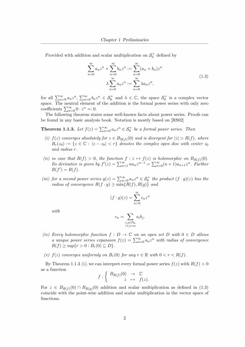
The following theorem states some well-known facts about power series. Proofs canbe found in any basic analysis book. Notation is mostly based on [RS02]
Theorem 1.1.3. Let f(z) =∑∞
n=0 anzn ∈ S+
0 be a formal power series. Then
(i) f(z) converges absolutely for z ∈ BR(f)(0) and is divergent for |z| > R(f), whereBr(z0) := z ∈ C : |z − z0| < r denotes the complex open disc with center z0
and radius r.
(ii) in case that R(f) > 0, the function f : z 7→ f(z) is holomorphic on BR(f)(0).Its derivative is given by f ′(z) =
∑∞n=1 nanz
n−1 =∑∞
n=0(n+ 1)an+1zn. Further
R(f ′) = R(f).
(iii) for a second power series g(z) =∑∞
n=0 anzn ∈ S+
0 the product (f · g)(z) has theradius of convergence R(f · g) ≥ minR(f), R(g) and
(f · g)(z) =
∞∑n=0
cnzn
withcn =
∑i,j∈N0i+j=n
aibj .
(iv) Every holomorphic function f : D → C on an open set D with 0 ∈ D allowsa unique power series expansion f(z) =
∑∞n=0 anz
n with radius of convergenceR(f) ≥ supr > 0 : Br(0) ⊆ D.
(v) f(z) converges uniformly on Br(0) for any r ∈ R with 0 < r < R(f).
By Theorem 1.1.3 (i), we can interpret every formal power series f(z) with R(f) > 0as a function
f :
BR(f)(0) → C
z 7→ f(z).
For z ∈ BR(f)(0) ∩ BR(g)(0) addition and scalar multiplication as defined in (1.3)coincide with the point-wise addition and scalar multiplication in the vector space offunctions.
2

Chapter 1 Preliminaries
Defintion 1.1.4. We define the formal differential operator on S+0 by
d :
S+
0 → S+0∑∞
n=0 anzn 7→
∑∞n=0(n+ 1)an+1z
n.
Theorem 1.1.3 (ii) shows that we can interpret every formal power series f , withR(f) > 0 as a holomorphic function f : BR(f)(0)→ C, where for z ∈ BR(f)(0)
(df)(z) = f ′(z).
Defintion 1.1.5. The product of two formal power series can be defined as( ∞∑n=0
anzn
)·
( ∞∑n=0
bnzn
):=
∞∑n=0
(n∑i=0
aibn−i
)zn.
For k ∈ N we are able to introduce the k-th power of a formal power series by induction( ∞∑n=0
bnzn
)1
:=
∞∑n=0
bnzn
( ∞∑n=0
bnzn
)k:=
( ∞∑n=0
bnzn
)k−1
·
( ∞∑n=0
bnzn
).
We write ( ∞∑n=0
bnzn
)k=∞∑n=0
b(k)n zn (1.4)
for the corresponding coefficients b(k)n . Further we define the zeroth power of a formal
power series by ( ∞∑n=0
bnzn
)0
:= 1.
By Theorem 1.1.3 (iii) we know that R(bk) ≥ R(b). The coefficients b(k)n can be
computed explicitly in the following way:
Theorem 1.1.6. For k ∈ N, the coefficients in (1.4) satisfy
b(k)n =
∑n1+n2+...+nk=n
(n1,...,nk)∈Nk0
bn1bn2 . . . bnk . (1.5)
Proof. For k = 1 we have( ∞∑n=0
bnzn
)1
=∞∑n=0
b(1)n zn =
∞∑n=0
bnzn.
3
Chapter 1 Preliminaries
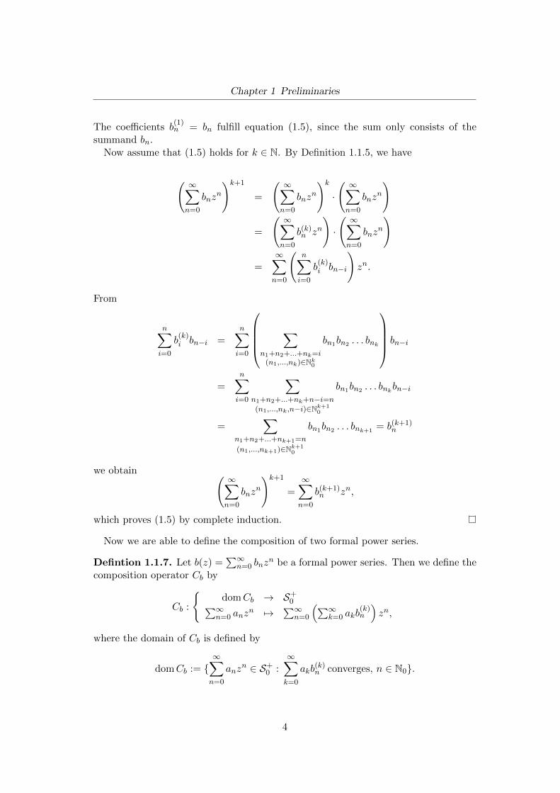
The coefficients b(1)n = bn fulfill equation (1.5), since the sum only consists of the
summand bn.Now assume that (1.5) holds for k ∈ N. By Definition 1.1.5, we have
( ∞∑n=0
bnzn
)k+1
=
( ∞∑n=0
bnzn
)k·
( ∞∑n=0
bnzn
)
=
( ∞∑n=0
b(k)n zn
)·
( ∞∑n=0
bnzn
)
=∞∑n=0
(n∑i=0
b(k)i bn−i
)zn.
From
n∑i=0
b(k)i bn−i =
n∑i=0
∑n1+n2+...+nk=i
(n1,...,nk)∈Nk0
bn1bn2 . . . bnk
bn−i
=n∑i=0
∑n1+n2+...+nk+n−i=n(n1,...,nk,n−i)∈Nk+1
0
bn1bn2 . . . bnkbn−i
=∑
n1+n2+...+nk+1=n
(n1,...,nk+1)∈Nk+10
bn1bn2 . . . bnk+1= b(k+1)
n
we obtain ( ∞∑n=0
bnzn
)k+1
=∞∑n=0
b(k+1)n zn,
which proves (1.5) by complete induction.
Now we are able to define the composition of two formal power series.
Defintion 1.1.7. Let b(z) =∑∞
n=0 bnzn be a formal power series. Then we define the
composition operator Cb by
Cb :
domCb → S+
0∑∞n=0 anz
n 7→∑∞
n=0
(∑∞k=0 akb
(k)n
)zn,
where the domain of Cb is defined by
domCb := ∞∑n=0
anzn ∈ S+
0 :∞∑k=0
akb(k)n converges, n ∈ N0.
4

Chapter 1 Preliminaries
Remark 1.1.8.
(i) Let b(z) =∑∞
n=0 bnzn be arbitrary and f(z) =
∑∞n=0 anz
n, g(z) =∑∞
n=0 cnzn
such that f, g ∈ domCb. Then
∞∑n=0
(ak + λck)b(k)n =
∞∑n=0
akb(k)n + λ
∞∑n=0
ckb(k)n
exists for λ ∈ C. Hence, domCb is a linear subspace of S+0 .
(ii) For f(z) = zk, k ∈ N,
(Cbf)(z) =∞∑n=0
b(k)n zn = b(z)k
shows, that the composition of zk with a formal power series b(z) coincides withthe k-th power of the formal power series b(z), as defined in Definition 1.1.5.
The following example shows, that in general domCb 6= S+0 :
Example 1.1.9. We define two formal power series by f(z) :=∑∞
n=0 zn, and b(z) :=
1+z. Then b(z)k =∑k
n=0
(kn
)zn. But the sum
∑∞k=0
(kn
)is divergent for all n ∈ N0.
Hence, f /∈ domCb.
Nevertheless, in the special case, that b(0) = 0, the domain of Cb is the whole space,as the following theorem shows:
Theorem 1.1.10. For b(z) =∑∞
n=0 bnzn =
∑∞n=1 bnz
n (i.e. b0 = 0) we havedomCb = S+
0 .
Proof. Let k ∈ N k > n. Then for every tuple (n1, n2, . . . , nk) ∈ Nk0 with n1 + n2 +. . . + nk = n, there exists at least one j ∈ 1, 2, . . . , k such that nj = 0. It followsfrom Theorem 1.1.6, that
b(k)n =
∑n1+n2+...+nk=n(n1,n2,...,nk)∈Nk0
bn1bn2 . . . bnk =∑
n1+n2+...+nk=n(n1,n2,...,nk)∈Nk0
0 = 0,
since b0 = 0. Hence, for any arbitrary complex sequence (an)n∈N0 ∈ CN0 , the sum∑∞k=0 akb
(k)n has only a finite number of non-zero summands. Therefore, it converges
and its sum coincides with∑n
k=0 akb(k)n . This shows that f(z) =
∑∞n=0 anz
n ∈ domCband we obtain domCb = S+
0 .
Lemma 1.1.11. Let b(z) =∑∞
n=0 bnzn and f(z) =
∑∞n=0 anz
n ∈ domCb. Then|b0| ≤ R(f).
5
Chapter 1 Preliminaries
Proof. Since f ∈ domCb, the series∑∞
n=0 b(n)k an converges for every k ∈ N0 by defi-
nition of domCb. In particular, this is true for k = 0. Because of b(n)0 = bn0 , we find
that∞∑n=0
b(n)0 an =
∞∑n=0
bn0an
converges. By Theorem 1.1.3, (i) this can only be the case if |b0| ≤ R(f).
Theorem 1.1.12. An arbitrary complex series∑∞
n,k=0 an,k converges absolutely if andonly if
∑∞k=0 |an,k| < +∞, for all n ∈ N0 and
∑∞n=0
∑∞k=0 |an,k| < +∞. In this case
∞∑n,k=0
an,k =∞∑n=0
∞∑k=0
an,k =∞∑k=0
∞∑n=0
an,k.
Proof. A proof can be found in [Rud70].
Lemma 1.1.13. Let b(z) =∑∞
n=0 bnzn, f(z) =
∑∞n=0 anz
n ∈ S+0 , such that R(b) > 0
and |b0| < R(f). Then f ∈ domCb and there exists a real number δ > 0, withδ ≤ R(Cbf), such that (Cbf)(z) = f(b(z)) for all z ∈ Bδ(0).
In this case for all real constants r > 0 such that r ≤ R(b) and b(Br(0)) ⊆ BR(f)(0),we have R(Cbf) ≥ r and (Cbf)(z) = f(b(z)) for all z ∈ Br(0).
Proof. We define a formal power series by
c(z) :=
∞∑n=0
cnzn :=
∞∑n=0
|bn|zn.
By Theorem 1.1.6, we have
|b(k)n | =
∣∣∣∣∣∣∣∣∑
n1+...+nk=n(n1,n2,...,nk)∈Nk
bn1 · ... · bnk
∣∣∣∣∣∣∣∣≤
∑n1+...+nk=n
(n1,n2,...,nk)∈Nk
|bn1 | · ... · |bnk |
=∑
n1+...+nk=n(n1,n2,...,nk)∈Nk
cn1 · ... · cnk = c(k)n ,
for k ∈ N.
If we recall the definition of the radius of convergence (1.2), it is clear, that R(c) =R(b) > 0. Since c(z) is continuous on BR(b)(0) and c(0) = |b0| < R(f) by assumption,there exists a δ ∈ R, 0 < δ < R(b) such that |c(z)| < R(f) for all z ∈ Bδ(0).
6

Chapter 1 Preliminaries
Using this, we can calculate for z0 ∈ Bδ(0)
∞∑n=0
∞∑k=0
∣∣∣anb(n)k zk0
∣∣∣ =∞∑n=0
|an|∞∑k=0
|b(n)k ||z0|n ≤
≤∞∑n=0
|an|∞∑k=0
c(n)k |z0|n =
∞∑n=0
|an|c(|z0|)n < +∞.
since c(|z0|) = |c(|z0|)| < R(f).
Furthermore, since |z0| < R(b), the series b (z0)n =∑∞
k=0 b(n)k zk0 converges absolutely
for every n ∈ N. So we can apply Theorem 1.1.12 to the series∑∞
n,k=0 anb(n)k zk0 and
obtain that∑∞
n=0 anb(n)k converges for all k ∈ N. Thus, f ∈ domCb. Moreover,
f(b(z0)) =∞∑n=0
an
∞∑k=0
b(n)k zk0 =
∞∑k=0
∞∑n=0
anb(n)k zk0 = (Cbf)(z0).
Now let r > 0 be such that b(Br(0)) ⊆ BR(f)(0). Then f(b(z)) is a holomorphicfunction on Br(0), since it is the composition of two holomorphic functions. Hence,by Theorem 1.1.3, (iv), it has a unique power series expansion f(b(z)) =
∑∞n=0 dnz
n.The radius of convergence of
∑∞n=0 dnz
n is at least r.
Let δ be as above. Since Cbf is holomorphic on Bδ(0), it has a unique power seriesexpansion
∑∞n=0 enz
n. We conclude that
∞∑n=0
dnzn = f(b(z)) = (Cbf)(z) =
∞∑n=0
enzn
for all z ∈ Bδ(0). Since the power series expansion is unique, dn = en follows for alln ∈ N0. Hence, Cbf has a radius of convergence of, at least, r and (Cbf)(z) = f(b(z))for all z ∈ Br(0).
Example 1.1.14. Let b(z) =∑∞
n=1 bnzn ∈ S+ be an arbitrary power series with R(b) >
0 and
Bµ(z) =
∞∑n=0
(µn
)zn (1.6)
denote the Binomial series, for an arbitrary complex number µ. The binomial coeffi-cients in (1.6) are defined by(
µn
):=
µ(µ−1)(µ−2)···(µ−n+1)
n! , n ∈ N1, n = 0.
It is well known, that
R(Bµ) =
+∞, µ ∈ N0
1, µ ∈ C \ N0
7
Chapter 1 Preliminaries
and Bµ(z) = (1 + z)µ for all z ∈ BR(Bµ)(0). Since b(0) = 0, we know by Theorem
1.1.10, that domCb = S+0 and hence Bµ(z) ∈ domCb.
Now let r > 0 be such that |b (z) | < 1 for all z ∈ Br(0). Then due to Lemma 1.1.13we have R(CbBµ) ≥ r and
(CbBµ) (z) = Bµ (b(z)) = (1 + b(z))µ ,
for all z ∈ Br(0).
This motivates the following definition.
Defintion 1.1.15. Let f(z) =∑∞
n=0 anzn ∈ S+
0 be an arbitrary power series witha0 6= 0 and µ ∈ C. Then we define the µ-th power of f(z) by
f(z)µ := aµ0 (CbBµ)(z)
where
b(z) :=
∞∑n=1
ana0zn.
Remark 1.1.16. Let f , b and µ be as before with R(f) > 0. Then because of R(b) =R(f) > 0 and b(0) = 0 Lemma 1.1.13 asserts, that R(fµ) > 0.
1.2 Spaces with indefinite inner product
Defintion 1.2.1. Let X be a complex vector space, and [·, ·] : X ×X → C a hermitianmapping (i.e. [x + λy, z] = [x, z] + λ[y, z] and [x, y] = [y, x] for x, y, z ∈ X , λ ∈ C).Then we call [·, ·] an inner product and the pair (X , [·, ·]) an inner product space.
Remark 1.2.2. Note, that for x ∈ X from [x, x] = [x, x] follows that [x, x] ∈ R.
Defintion 1.2.3. An element x ∈ X is called
positive ⇔ [x, x] > 0negative ⇔ [x, x] < 0neutral ⇔ [x, x] = 0
isotropic ⇔ [x, y] = 0, y ∈ X .
We denote the set of all isotropic elements by X and call it the isotropic part of(X , [·, ·]).
An inner product space is called positive (negative) definite if all elements exceptfor the zero vector are positive (negative) elements. It is called positive (negative)semidefinite if it has no negative (positive) elements. Otherwise it is called indefinite.X is called degenerated if X 6= 0. Otherwise it is called non-degenerated.
Remark 1.2.4. If Y ≤ X is a linear subspace of an inner product space (X , [·, ·]), then(Y, [·, ·]) is an inner product space itself. We call the subspace Y positive/negative(semi)definite if (Y, [·, ·]) is positive/negative (semi)definite.
8
Chapter 1 Preliminaries
Lemma 1.2.5. The isotropic part X of an inner product space (X , [·, ·]) is a linearsubspace of X . Every element of X is neutral.
Proof. For x, y ∈ X and arbitrary z ∈ X , λ ∈ C we have
[x+ λy, z] = [x, z] + λ[y, z] = 0.
Hence X is a linear subspace. The second assertion is clear.
Example 1.2.6. Every Hilbert space (H, 〈·, ·〉) is a positive definite inner product space.
Remark 1.2.7. Since X is a linear subspace of X , the factor space X/X is again avector space. If we endow X/X with the inner product
[x+ X , y + X ]/X := [x, y] (1.7)
the space (X/X , [·, ·]/X ) is again an inner product space. Note, that [·, ·]/X is her-mitian, since [·, ·] is hermitian. It is well-defined, since for x1, x2, y1, y2 ∈ X such thatx1 − x2, y1 − y2 ∈ X , we have [x2 − x1, y1] = 0 and there follows
[x1 + X , y1 + X ]/X − [x2 + X , y2 + X ]/X =
= [x1, y1]− [x2, y2] = [x1, y1]− [x2, y2]− [x1 − x2, y1] =
= [x2, y1 − y2] = 0.
Let x+X ∈ X/X such that [x+X , y+X ]/X = 0 for all y+X ∈ X/X . Then
0 = [x+ X , y + X ]/X = [x, y]
for all y ∈ X shows, that x ∈ X and hence (X/X ) = 0. Thus X/X is non-degenerated.
Example 1.2.8. Let (X1, [·, ·]1), (X2, [·, ·]2) be positive semidefinite inner product spaces.Then we define (X , [·, ·]) by X := X1 ×X2 and
[(x1, x2), (y1, y2)] := [x1, y1]1 − [x2, y2]2 .
Since [·, ·]1 and [·, ·]2 are inner products, [·, ·] is an inner product as well. Let ι1, ι2denote the embeddings of X1, X2 into X . Then, since X1, X2 are positive semidefinite,
[ι1(x1), ι1(x1)] = [x1, x1]1 − [0, 0]2 = [x1, x1]1 ≥ 0
and[ι2(x2), ι2(x2)] = [0, 0]1 − [x2, x2]2 = −[x2, x2]2 ≤ 0
for all x1 ∈ X1, x2 ∈ X2. Hence ι1(X1) is a positive semidefinite and ι2(X2) a negativesemidefinite subspace of X .
If (x1, x2) ∈ X is isotropic, we have
0 = [(x1, x2), (y1, y2)] = [x1, y1]1 − [x2, y2]2 (1.8)
for all (y1, y2) ∈ X . Hence x1 ∈ X 1 and x2 ∈ X 2 . If, on the other hand x1 ∈ X 1 andx2 ∈ X 2 , equation (1.8) holds for all (y1, y2) ∈ H. Thus,
X = X 1 ×X 2 .
9

Chapter 1 Preliminaries
Defintion 1.2.9. We call two elements x, y ∈ X of an inner product space (X , [·, ·])orthogonal if [x, y] = 0 and denote this by x[⊥]y. Two subspaces X1,X2 ≤ X are calledorthogonal if x1[⊥]x2 for all x1 ∈ X1, x2 ∈ X2, and we denote this fact by X1[⊥]X2.
The orthogonal complement M [⊥] of a set M ⊆ X is defined as
M [⊥] := x ∈ X : x[⊥]m, m ∈M.
A linear operator P : X → X is called a projection if it is idempotent (i.e. P 2 = P ).A projection is called orthogonal (with respect to [·, ·]) if ranP [⊥] kerP .
Lemma 1.2.10. Let (X , [·, ·]) be an inner product space and X1,X2 ≤ X subspaces ofX , such that
X1 u X2 = X (1.9)
(the symbol u denotes a direct sum i.e. X1 +X2 = X and X1 ∩X2 = 0). Then thereexist unique linear projection operators Pi : X → Xi, i = 1, 2, with PiXi = Xi andkerPi = X1−i
If the spaces are such that
X1[u]X2 = X (1.10)
(i.e. X1 u X2 = X and X1[⊥]X2), the projectors Pi are orthogonal.
Proof. For x ∈ X exist x1 ∈ X1, x2 ∈ X2, such that x = x1 + x2. This decompositionis unique: For y1 ∈ X1, y2 ∈ X2 with y1 + y2 = x, we have
0 = x1 − y1 + x2 − y2.
Since x1 − y1 ∈ X1 and x2 − y2 ∈ X2 and X1 ∩ X2 = 0,
x1 − y1 = x2 − y2 = 0.
Now we define Pix := xi for i = 1, 2. Because of
Pi(x1 + x2 + λ(y1 + y2)) = xi + λyi = Pi(x1 + x2) + λPi(y1 + y2)
for xi, yi ∈ Xi, λ ∈ C they are linear, and since P 2i x = Pixi = xi = Pix, they are
projections. The kernel of P1 is
ker P1 = x ∈ X : P1x = 0 = X2
and vice versa.
Let Q 6= 0 be linear a projection on Xi. Then
Pi(x1 + x2)−Q(x1 + x2) = xi − xi = 0
shows that Q = Pi. Hence, if X1[⊥]X2, the projectors are orthogonal.
10

Chapter 1 Preliminaries
Defintion 1.2.11. Let (X , [·, ·]) be an inner product space and X+, X− subspaces ofX such that
X = X+[u]X−[u]X.
Then we call the space X decomposable and the pair (X+,X−) a fundamental decom-position of X . The linear operator
J :
X → Xx 7→ P+x− P−x,
where P± denote the projections onto X±, is called fundamental symmetry or met-ric operator. If we want to emphasize, that a fundamental symmetry J belongs tothe fundamental decomposition (X+,X−), we will also call the triplet (X+,X−, J) afundamental decomposition of X .
Lemma 1.2.12. For a fundamental decomposition (X+,X−, J) of an indefinite innerproduct space (H, [·, ·]),
(i) [x, y] = [P+x, y] + [P−x, y]
(ii) [P±x, y] = [x, P±y] = [P±x, P±y]
(iii) [Jx, y] = [x, Jy]
(iv) [x, y] = [Jx, Jy] = [JJx, y]
hold for x, y ∈ X
Proof. (i): Let x ∈ X such that x = (P+ + P−)x+ x. Then
[x, y] = [P+x, y] + [P−x, y] + [x, y] = [P+x, y] + [P−x, y].
(ii): Follows from X+ ⊥ X−.(iii):
[Jx, y] = [P+x, y]− [P−x, y] = [x, P+y]− [x, P−y] = [x, Jy]
(iv):
[Jx, Jy] = [P+x, P+y]− [P+x, P−y]− [P−x, P+y] + [P−x, P−y] =
= [P+x, P+y] + [P−x, P−y] = [P+x, y] + [P−x, y] = [x, y].
The second equality follows from (iii).
Example 1.2.13. Recall the indefinite inner product space from Example 1.2.8 andassume this time, that X1,X2 are positive definite. Then, since X = 0 and
[ι1(x), ι2(y)] = [(x, 0), (0, y)] = [x, 0]1 − [0, y]2 = 0,
(ι1(X1), ι2(X2)) is a fundamental decomposition. The action of J is given by J(x1, x2) =(x1,−x2).
11
Chapter 1 Preliminaries
Defintion 1.2.14. Let (X , [·, ·]) be an inner product space and (X+,X−, J) a funda-mental decomposition. Then we define a mapping by
[·, ·]J :
X × X → C
(x, y) 7→ [Jx, y]
and call it the inner product induced by the fundamental decomposition (X+,X−, J).
Lemma 1.2.15. Let (X , [·, ·]) and (X+,X−, J), be again an inner product space andan arbitrary fundamental decomposition. Then [·, ·]J is a positive semidefinite innerproduct. Moreover
(X , [·, ·]) = (X , [·, ·]J)
and (X , [·, ·]J) is positive definite if and only if (X , [·, ·]) is non degenerated.
Proof. Since J is linear, [·, ·]J is linear in the first argument and because of
[x, y]J = [Jx, y] = [x, Jy] = [Jy, x] = [y, x]J
by Lemma 1.2.12, (iii), for all x, y ∈ X , it is hermitian. It is also positive semidefinite,since for x ∈ X
[x, x]J = [Jx, x] = [P+x, x]− [P−x, x] = [P+x, P+x]− [P−x, P−x] ≥ 0.
Now let x ∈ (X , [·, ·]). Then by Lemma 1.2.12, (iii),
[x, y]J = [Jx, y] = [x, Jy] = 0
for all y ∈ X and hence (X , [·, ·]) ⊆ (X , [·, ·]J).
For x ∈ (X , [·, ·]J) we have
[x, y] = [Jx, Jy] = [x, Jy]J = 0
for all y ∈ X due to Lemma 1.2.12, (iv), and thus (X , [·, ·]) ⊇ (X , [·, ·]J). The lastassertion is clear since the isotropic parts coincide.
Remark 1.2.16. Since the inner product [·, ·]J is positive semidefinite, it induces asemi-norm ‖ · ‖J on X by
‖x‖2J := [x, x]J
for all x ∈ X . By Lemma 1.2.15 ‖ · ‖J is a norm if and only if (X, [·, ·]) is non-degenerated.
Defintion 1.2.17. Let (K, [·, ·]) be a decomposable, non-degenerated inner productspace and assume that there exists a fundamental symmetry J such that (K, [·, ·]J) iscomplete. Then we call (K, [·, ·]) a Krein space.
12

Chapter 1 Preliminaries
Example 1.2.18. Consider again the inner product space from Examples 1.2.8 and1.2.13. This time assume, that X = H1 × H2 = ι1(H1)[u]ι2(H2), where (H1, 〈·, ·〉1),(H2, 〈·, ·〉2) are Hilbert spaces. Now let ((xn, yn))n∈N be a Cauchy series in X . Thenbecause of
‖(xn, yn)− (xm, ym)‖2J = [(xn − xm, yn − ym), (xn − xm, yn − ym)]J
= [xn − xm, xn − xm]1 + [yn − ym, yn − ym]2
= ‖xn − xm‖21 + ‖yn − ym‖22,
the series (xn)n∈N, (yn)n∈N are Cauchy in H1 and H2 respectively. Since H1 and H2
are complete, there exist x ∈ H1 and y ∈ H2 such that limn→∞ ‖xn − x‖1 = 0 andlimn→∞ ‖yn − y‖2 = 0. Thus,
limn→∞
‖(xn, yn)− (x, y)‖2J = limn→∞
‖xn − x‖21 + limn→∞
‖yn − y‖21 = 0.
Hence, (X , [·, ·]J) is complete and (X , [·, ·]) is a Krein space.
Lemma 1.2.19. Let (X , [·, ·]) be a semidefinite inner product space. Then
(i) X = x ∈ X : x is neutral
(ii) for x, y ∈ X the Cauchy-Schwartz inequality
|[x, y]| ≤√
[x, x][y, y] (1.11)
holds.
Proof. If (X , [·, ·]) is negative semidefinite, we just consider the positive semidefiniteinner product space (X ,−[·, ·]). So we can assume without loss of generality, that(X , [·, ·]) is positive semidefinite.
Let x, y ∈ X be arbitrary such that [x, y] 6= 0. For λ ∈ R we have
0 ≤[x− λy [x, y]
|[x, y]|, x− λy [x, y]
|[x, y]|
]= [x, x]− λ [x, y]
|[x, y]|[y, x]− λ [y, x]
|[x, y]|[x, y] + λ2[y, y]
= [x, x]− 2λ|[x, y]|+ λ2[y, y].
(1.12)
We already know that X ⊆ x ∈ X : x is neutral. Assume that y is neutral
and [x, y] 6= 0 for some x ∈ X . Then, because of [y, y] = 0, choosing λ > [x,x]2|[x,y]| in
inequality (1.12) leads to
0 ≤ [x, x]− 2λ|[x, y]| < [x, x]− [x, x] = 0.
Hence, [x, y] = 0 for all x ∈ X and therefore y ∈ X , which shows (i).
If x or y are isotropic, inequality (1.11) is fulfilled. For x, y /∈ X , setting λ = |[x,y]|[y,y]
in inequality (1.12) asserts
0 ≤ [x, x]− |[x, y]|2
[y, y],
which is equivalent to (1.11).
13
Chapter 1 Preliminaries
Lemma 1.2.20. Let (K, [·, ·]) be an inner product space and (K+,K−, J) some funda-mental decomposition. Then for M ⊆ K, the set M [⊥] is a linear subspace of K andM [⊥] is closed with respect to ‖ · ‖J .
Proof. For x ∈M , we define a linear mapping by
fx :
K → Cy 7→ [x, y].
Then we can write M [⊥] as
M [⊥] =⋂x∈M
ker fx.
Because of
|fx(y)|2 = |[x, y]|2 = |[Jx, y]J |2 ≤ ‖Jx‖J‖y‖Jfor all x, y ∈ K, the mappings fx are continuous with respect to ‖ · ‖J and each ker fxis a closed subspace of (K, [·, ·]J). Hence, M [⊥] is a closed subspace as well.
Remark 1.2.21. The proof in Lemma 1.2.20 works also for for an arbitrary innerproduct space (X , [·, ·]) and a norm ‖ · ‖ on X , such that fx is continuous for allx ∈ X .
Since we will use it in the proof of the following lemma, we present a formulation ofthe closed graph theorem (without proof).
Theorem 1.2.22 (Closed graph theorem). Let (X , ‖·‖X ), (Y, ‖·‖Y) be Banach spacesand T : X → Y a linear operator. Then T is continuous if and only if the graph of T(i.e. the set (x, y) ∈ X ×Y : y = Tx) is closed in X ×Y, endowed with the producttopology.
Proof. Can be found in [Rud70].
Lemma 1.2.23. Let K be a Krein space and (K+,K−, J) be the fundamental decom-position such that (K, [·, ·]J) is complete. Further, let (K′+,K′−, J ′) be an arbitraryfundamental decomposition. Then there exists a real constant C > 0, such that
‖JJ ′x‖J ≤ C‖x‖J (1.13)
and
‖J ′Jx‖J ′ ≤ C‖x‖J ′ (1.14)
for all x ∈ X
Proof. To prove inequality (1.13), we first note that, because of
‖Jx‖2J = [JJx, Jx] = [Jx, x] = [x, x]J = ‖x‖2J ,
the operator J is an isometry with respect to ‖ · ‖J and therefore continuous. Now let(xn)n∈N be a series in K such that limn→∞ ‖xn−x‖J = 0 and limn→∞ ‖P ′+xn−y‖J = 0
14
Chapter 1 Preliminaries
for some x, y ∈ K. Then, since by Lemma 1.2.20 K′+ =(K′−)[⊥]
is closed, we have
y ∈ K′+. Moreover, because P ′+xn − xn ∈ K′−, and K′− =(K′+)[⊥]
is closed as well, weobtain
limn→∞
P ′+xn − xn = y − x ∈ K′−.
Now0 = P ′+(y − x) = y − P ′+x
shows, that P ′+x = y. Thus P ′+ is closed with respect to ‖ · ‖J . By the closed graphtheorem, it is continuous. It can be shown analogously, that P ′− is continuous withrespect to ‖ · ‖J as well. Since JJ ′ = J(P ′+ − P ′−) is the composition of continuousmappings, it is continuous itself. Hence, there exists a real constant C > 0, such that(1.13) holds.
To prove inequality (1.14), we first show by complete induction, that∥∥J ′Jx∥∥2n
J ′≤∥∥(J ′J)2nx
∥∥J ′‖x‖2
n−1J ′ (1.15)
holds for every n ∈ N. By the Cauchy-Schwartz inequality and Lemma 1.2.12, we find∥∥J ′Jx∥∥2
J ′=
[J ′Jx, J ′Jx
]J ′
=[J ′Jx, Jx
]=
[J ′J ′JJ ′Jx, x
]=
[(J ′J)2x, x
]2J ′≤∥∥(J ′J)2x
∥∥J ′‖x‖J ′ ,
for all x ∈ K. But this is nothing else, but inequality (1.15) with n = 1.Now assume, that (1.15) holds for some n ∈ N. Then for x ∈ K∥∥J ′Jx∥∥2n+1
J ′=
(∥∥J ′Jx∥∥2n
J ′
)2
≤(∥∥(J ′J)2nx
∥∥ ‖x‖2n−1J ′
)2
=∥∥(J ′J)2nx
∥∥2 ‖x‖2n+1−2J ′
=[(J ′J)2nx, (J ′J)2nx
]J ′‖x‖2
n+1−2J ′
=[(JJ ′)2n
J ′(J ′J)2n
x, x]‖x‖2
n+1−2J ′
=[(J ′J)2n+1
x, x]J ′‖x‖2
n+1−2J ′
≤∥∥∥(J ′J)2n+1
x∥∥∥J ′‖x‖J ′ ‖x‖
2n+1−2J ′ =
∥∥∥(J ′J)2n+1x∥∥∥J ′‖x‖2
n+1−1J ′ ,
shows that (1.15) holds for all n ∈ N. From the previously proven inequality (1.13),we derive ∥∥(J ′J)2nx
∥∥2
J ′=
[(J ′J)2nx, (J ′J)2nx
]J ′
= [(J ′J)2nx, J(J ′J)2n−1x]
= [J(J ′J)2nx, J(J ′J)2n−1x]J
≤ ‖(JJ ′)2nJx‖J‖(JJ ′)2n−1Jx‖J≤ C2n‖Jx‖JC2n−1‖Jx‖J = C2n+1−1‖x‖2J .
15

Chapter 1 Preliminaries
Combining this with (1.15) yields
∥∥J ′Jx∥∥J ′≤(∥∥(J ′J)2nx
∥∥ ‖x‖2n−1J ′
)2−n
≤
≤(C2n− 1
2 ‖x‖J ‖x‖2n−1J ′
)2−n
= C1−2−n−1‖x‖2−nJ ‖x‖1−2−n
J ′
for all n ∈ N. For n→∞ on the right hand side we obtain inequality (1.14).
Theorem 1.2.24. Let K be a Krein space. Then two norms induced by fundamentalsymmetries are equivalent.
Proof. Let (K+,K−, J) be the fundamental decomposition such that (K, [·, ·]J) is com-plete and (K′+,K′−, J ′) an arbitrary fundamental decomposition. Then it is sufficientto show that ‖ · ‖J and ‖ · ‖J ′ are equivalent, i.e. there exist real constants λ1, λ2 > 0,such that
λ1‖x‖J ′ ≤ ‖x‖J ≤ λ2‖x‖J ′for all x ∈ X .
Since (X , [·, ·]J) is positive definite, by the Cauchy-Schwartz inequality, Lemma1.2.12 and Lemma 1.2.23 we have
‖x‖2J ′ = [J ′x, x] = [JJ ′x, x]J ≤ ‖JJ ′x‖J‖x‖J ≤ C‖x‖2J . (1.16)
Inequality (1.16) also holds if we switch J and J ′. Thus, we obtain
1√C‖x‖J ′ ≤ ‖x‖J ≤
√C‖x‖J ′ .
Corollary 1.2.25. Let (X , [·, ·]) be an inner product space. Then the following state-ments are equivalent:
(i) (X , [·, ·]) is a Krein space.
(ii) There exists a fundamental decomposition (H1,H2, J) such that (H1, [·, ·]) and(H2,−[·, ·]) are Hilbert spaces.
Proof. (ii)⇒ (i):We’ve already established that in Examples 1.2.8, 1.2.13 and 1.2.18.
(i)⇒ (ii):Let (X+,X−, J) be a fundamental decomposition, such that (X , [·, ·]J) is complete.Since for x ∈ X+, y ∈ X− we have
[x, x] = [Jx, x] ≥ 0
−[y, y] = [Jy, y] ≥ 0
the spaces (X+, [·, ·]) and (X−,−[·, ·]) are positive semidefinite. Moreover, becauseby definition (X , [·, ·]) is non-degenerated and all neutral elements are isotropic byLemma 1.2.19, (X ; [·, ·]) and (X−,−[·, ·]) are positive definite. Since X+ = (X−)⊥ andvice versa, they are closed with respect to ‖ · ‖J and, therefore, Hilbert spaces.
16

Chapter 1 Preliminaries
Since we will need it later on, we define contraction operators on (indefinite) innerproduct spaces as follows:
Defintion 1.2.26. Let (X , [·, ·]) be an inner product space, and T : X → X be alinear operator. Then we call T a contraction if
[Tx, Tx] ≤ [x, x]
for all x ∈ X .
Note that, if [·, ·] is positive definite, T being a contraction is equivalent to T beinga bounded linear operator with norm smaller or equal 1.
Defintion 1.2.27. A Krein space H1[u]H2 such that mindimH1, dimH2 < +∞ iscalled Pontryagin space.
1.3 Defect operators
Defintion 1.3.1. Let (H, 〈·, ·〉H)H be a Hilbert space and T : H → H a boundedlinear operator. Then we denote the family of all such operators by B(H). We callT ∈ B(H) a contraction if
‖Tx‖H ≤ ‖x‖H
for all x ∈ H (i.e. ‖T‖ ≤ 1).
Further we define the space H(T ) by
H(T ) := ranT = x ∈ H : ∃y ∈ H : x = Ty .
Since for every x ∈ HT−1x = y+ kerT,
for any y ∈ T−1x and kerT is a closed subspace of H, the set T−1x is closed in H.Hence there exists a unique yx ∈ H with
‖yx‖H = min ‖y‖H : x = Ty
and we can define an inner product and norm on H(T ) by
〈x, z〉H(T ) := 〈yx, yz〉H , ‖x‖2H(T ) := ‖yx‖2H = 〈yx, yx〉H .
Remark 1.3.2. Note that yx = y−Py for any y ∈ T−1x, where P denotes the orthog-onal projection on kerT . Therefore yx is the unique element of T−1x ∩ (kerT )⊥.
Since ranT ∗ ⊆ (kerT )⊥
‖TT ∗x‖H(T ) = ‖T ∗x‖H
follows for all x ∈ H.
17

Chapter 1 Preliminaries
It is easy to check, that(H(T ), 〈·, ·〉H(T )
)is again a Hilbert space.
Let (H, 〈·, ·〉H)H be a Hilbert space and T : H → H be a contraction operator onH, then because of (I denotes the identity on H)
〈(I − TT ∗)x, x〉H = ‖x‖2H − 〈TT ∗x, x〉H = ‖x‖2H − ‖T ∗x‖2H ≥≥ ‖x‖2H
(1− ‖T ∗‖2H
)= ‖x‖2H
(1− ‖T‖2H
)≥ 0,
the operator I − TT ∗ is positive. In particular there exists a unique, self-adjoint andnon-negative square-root (I − TT ∗)
12 ∈ B(H).
Defintion 1.3.3. Let H be a Hilbert space, and T : H → H a linear contractionoperator. Then we call the operators
DT := (I − T ∗T )12 , DT ∗ := (I − TT ∗)
12
the defect operators and the Hilbert spaces
DT := H(DT ), DT ∗ := H(DT ∗)
the defect spaces of the operator T .
Theorem 1.3.4. Let H be a Hilbert space, and T : H → H a linear contractionoperator. Then x ∈ H is an element of DT ∗ if and only if
supy∈H
(‖x+ Ty‖2H − ‖y‖2H
)< +∞
In this case we can calculate the DT ∗-norm by
‖x‖2DT∗ = supy∈H
(‖x+ Ty‖2H − ‖y‖2H
)Proof. See [NV91], Chapter 1.
Remark 1.3.5.
(i) Since for x ∈ DT ∗
‖x‖D∗T = supy∈H
(‖x+ Ty‖2H − ‖y‖2H
)≥ ‖x+ T0‖2H − ‖0‖2H = ‖x‖2H
the embedding
ι :
DT ∗ → Hx 7→ x
is a contraction.
18

Chapter 1 Preliminaries
(ii) Because of
‖D2T ∗x‖2DT∗ = ‖DT ∗D
∗T ∗x‖2DT∗
= ‖D∗T ∗x‖2H=
⟨(I − TT ∗)
12 x, (I − TT ∗)
12 x⟩2
H= 〈(I − TT ∗)x, x〉H= ‖x‖2H − ‖T ∗x‖2H ≤ ‖x‖2H
for all x ∈ H, the operator D2T ∗ : H → DT ∗ is a contraction as well.
Lemma 1.3.6. Let T be a self-adjoint operator on a Hilbert space H, and P anarbitrary dense subset of H. Then the set D2
T ∗P is dense in DT ∗.
Proof. Let f = Tg ∈ H (T ) be arbitrary. Since T is continuous and self-adjoint,we can decompose the space H into the closed linear subspaces ranT u kerT =ranT u (ranT )⊥, and denote the orthogonal projections on kerT and ranT by Pkand Pr respectively. Then since Prg ∈ ranT there exists h ∈ H such that Th = Prg.Moreover since h ∈ H and P is dense in H, there exists a sequence (pn)n∈N, such thatlimn∈N ‖pn − h‖D = 0. Now we define (fn)n∈N :=
(T 2pn
)n∈N ⊆ T
2P.
Because of
‖fn − f‖H(T ) = ‖T 2pn − Tg‖H(T ) = ‖T (Tpn − g)‖H(T ) =
= mink∈kerT
‖Tpn − g + k‖D = mink∈kerT
‖Tpn − Prg − Pkg + k‖D ≤
≤ ‖Tpn − Th‖H + mink∈kerT
‖Pkg + k‖H ≤ ‖T‖‖pn − h‖H
limn→∞ ‖fn − f‖H(T ) = 0. Hence T 2P is dense in H(T ), since f was arbitrary.
1.4 Reproducing Kernel Hilbert spaces
For an arbitrary, non-empty set X, we denote the set of all functions from X to C byCX . If we define the addition of f, g ∈ CX by (f + g)(x) := f(x) + g(x) and the scalarmultiplication of f ∈ CX with λ ∈ C as (λf)(x) := λf(x) for all x ∈ X, then CX is avector space.
For every x ∈ X we can define the mapping
ιx :
CX → Cf 7→ f(x).
Because of ιx(λf + g) = λf(x) + g(x) = λιxf + ιxg for f, g ∈ CX , λ ∈ C, the mappingιx is linear.
19
Chapter 1 Preliminaries
Defintion 1.4.1. Let X be an arbitrary set and (H, 〈·, ·〉H) be a Hilbert space, suchthat H ≤ CX i.e. H is a linear subspace of CX . The space H is called a reproducingkernel Hilbert space (or RKHS) over X if ιx ∈ H′ for all x ∈ X, where the symbol H′denotes the topological dual space of H, defined by
H′ := h : H → C∣∣h is linear and continuous.
Lemma 1.4.2. Let (H, 〈·, ·〉H)H be a RKHS over X, then there exists a kernel functionKH : X ×X → C, such that for all w ∈ X the function KH(·, w) ∈ H and KH has thereproducing property:
f(w) = 〈f,KH(·, w)〉H (1.17)
for all f ∈ H.
Proof. Let w be an arbitrary element of X. Since H is a RKHS, ιw ∈ H′ and bythe Riesz representation theorem there exists a unique kw ∈ H, such that 〈f, kw〉H =ιwf = f(w) for all f ∈ H. Now we define our kernel function as
KH(z, w) := kw(z).
The existence of a kernel function is already a sufficient condition for a Hilbert spaceto be a RKHS.
Lemma 1.4.3. Let (H, 〈·, ·〉H)H be an arbitrary Hilbert space, such that H ≤ CX fora non-empty set X. Assume that there exists a kernel function KH : X ×X → C withKH(·, w) ∈ H, for all w ∈ X such that KH fulfills the reproducing property (1.17).Then H is a RKHS over X.
Proof. If we have 〈f,KH(·, w)〉H = f(w) = ιwf for f ∈ H, w ∈ X, the functional ιwis bounded by the Cauchy-Schwartz inequality.
If H is a RKHS, the following lemma shows that H(T ) has the same structure.
Theorem 1.4.4. Let (H, 〈·, ·〉H)H be a RKHS over a set X with reproducing kernel
K and T : H → H be a bounded linear operator. Then the space(H(T ), 〈·, ·〉H(T )
)is
again a RKHS with reproducing kernel KH(T )(·, w) := TT ∗K(·, w).
Proof. For fixed w, the function KH(T )(·, w) is an element of H(T ). So it is only leftto show, that KH(T ) has indeed the reproducing property. For this purpose let w ∈ X,
f ∈ H(T ) and g ∈ H such that f = Tg and g ∈ (kerT )⊥. Now we calculate⟨f,KH(T )(·, w)
⟩H(T )
= 〈Tg, TT ∗K(·, w)〉H(T ) = 〈g, T ∗K(·, w)〉H
since ranT ∗ ⊆ kerT⊥, and further
〈g, T ∗K(·, w)〉H = 〈Tg,K(·, w)〉H = 〈f,K(·, w)〉H = f(w).
20

Chapter 1 Preliminaries
Defintion 1.4.5. Let (H, 〈·, ·〉) be a Hilbert space. Then we call T ≤ H×H a linearrelation. If T is a closed subspace of H ×H it is called a closed linear relation. Theadjoint of T is defined by
T ∗ :=
(x, y) ∈ H ×H∣∣ 〈u, y〉 = 〈x, v〉 , (u, v) ∈ T
. (1.18)
Remark 1.4.6.
(i) Every linear operator T : H → H can be viewed as a linear relation if we identifyT with its graph.
(ii) The adjoint of the graph of a linear operator T as defined in (1.18) coincideswith the graph of the adjoint operator T ∗.
(iii) For any linear relation R
R∗∗ = R, R∗
= R∗.
For a proof and more on linear relations and their adjoint see [Kal14].
Lemma 1.4.7. Let (H, 〈·, ·〉H)H be a RKHS over a set X with reproducing kernel Kand b : X → X be a function such that the linear operator C defined by Cf := f bmaps into H. Then C∗ = span (K(·, w);K(·, b(w)) : w ∈ X) if we identify C withits graph.
If in addition C is a contraction
KH(T )(z, w) := K(z, w)−K(b(z), b(w))
is the reproducing kernel of the space H(T ), with T := (I − CC∗)12 .
Proof. We define R := span (K(·, w),K(·, b(w)) : w ∈ X). Then R is a closed sub-space of H × H and therefore a closed linear relation. A pair (f ; g) ∈ H × H bydefinition of the adjoint linear relation is an element of R∗ =
(R)∗
if and only if
〈g, u〉H = 〈f, v〉H (1.19)
for all (u; v) ∈ R. By definition of R, we have
(u; v) =
(N∑n=1
λnK(·, wn);N∑n=1
λnK(·, b(wn))
)
for some N ∈ N, λn ∈ C, wn ∈ X. Hence, if (f ; g) ∈ R∗
g(w) = 〈g,K(·, w)〉H = 〈f,K(·, b(w))〉H = f(b(w)) = (Cf)(w)
for all w ∈ X. Thus we have R∗ ⊆ C. On the other hand f b = Cf together withthe reproducing property yields
〈f,K(·, b(w))〉H = f(b(w)) = 〈f b,K(·, w)〉H .
21

Chapter 1 Preliminaries
By linearity (1.19) is fulfilled for all (u; v) ∈ R, and therefore R∗ = C. We conclude
C∗ = (R∗)∗ =((R)∗)∗
= R.
To prove the second assertion we calculate the kernel of H(T ) by Theorem 1.4.4 andobtain
KH(T )(z, w) = (TT ∗K(·, w)) (z) = ((I − CC∗)K(·, w))(z) =
= K(z, w)− (CK(·, b(w)))(z) = K(z, w)−K(b(z), b(w)).
22

Chapter 2
The Bergman and the Dirichlet space
2.1 The Bergman Space
Lemma 2.1.1. Let (H, 〈·, ·〉H) be a (complex) Hilbert space, X an arbitrary (complex)vector space and ψ : H → X a linear bijection. Then (X, 〈·, ·〉X) is a Hilbert space,where the inner product is defined as
〈·, ·〉X :
X ×X → C
(x, y) 7→⟨ψ−1(x), ψ−1(y)
⟩H .
The mapping ψ is isometric.
Proof. First note, that 〈·, ·〉X is sesquilinear, conjugate symmetric and non-negative,since it is the composition of a conjugate symmetric, non-negative sesquilinear formand a linear mapping.
Let x ∈ X, such that 〈x, x〉X = 0. Since
0 = 〈x, x〉X =⟨ψ−1(x), ψ−1(x)
⟩H
and 〈·, ·〉H is positive definite, we get that ψ−1(x) = 0 and hence x ∈ ker ψ. Due tothe fact that ψ is one-to-one, we have that x = 0. This shows that 〈·, ·〉X is positivedefinite.
Because for arbitrary x ∈ X
‖ψ(x)‖2X = 〈ψ(x), ψ(x)〉X =⟨ψ−1(ψ(x)), ψ−1(ψ(x))
⟩H = 〈x, x〉H = ‖x‖2H,
the mapping ψ is in fact an isometric isomorphism.
Now let (xn)n∈N be a Cauchy series in X, i.e.
∀ ε > 0∃N0 ∈ N : ‖xn − xm‖X < ε, ∀m,n ≥ N0.
Since ψ is isometric, the series(ψ−1(xn)
)n∈N is a Cauchy series in H. Because of the
completeness of H it converges to some h ∈ H. Now
‖xn − ψ(h)‖X = ‖ψ−1(xn)− h‖H
shows that xn → ψ(h), and hence X is complete.
23

Chapter 2 The Bergman and the Dirichlet space
Let CN0 =
(an)n∈N0: an ∈ C, n ∈ N0
denote the set of all complex series.
With addition and scalar multiplication defined by
(an)n∈N0+ (bn)n∈N0
:= (an + bn)n∈N0(2.1)
λ (an)n∈N0:= (λan)n∈N0
(2.2)
for (an)n∈N0, (bn)n∈N0
∈ CN0 , λ ∈ C, the set CN0 is a complex vector space. Theneutral element of the addition is the series (0)n∈N0 .
It is a well known fact, that the linear subspace l2 ≤ CN0 , defined by
l2 :=
(an)n∈N0
∈ CN0 :∞∑n=0
|an|2 < +∞
,
equipped with the inner product
〈·, ·〉l2 :
l2 × l2 → C(
(an)n∈N0, (bn)n∈N0
)7→
∑∞n=0 anbn
is a Hilbert space.
Defintion 2.1.2. Let the mapping ψ be defined by
ψ :
CN0 → S+
0
(an)n∈N0 7→∑∞
n=0
√n+ 1 anz
n.
The space(A2, 〈·, ·〉A2
), with A2 := ψ(l2) and 〈ψ(a), ψ(b)〉A2 := 〈a, b〉l2 is called
Bergman space.
Theorem 2.1.3. The Bergman space(A2, 〈·, ·〉A2
), is a RKHS over the open unit disc
D := R1(0) with kernel function
KA2(z, w) :=∞∑n=0
(n+ 1)wnzn.
Proof. To show, that A2 is in fact a Hilbert space, we’d like to apply Lemma 2.1.1.So we have to verify its assumptions. We already know, that l2 is a Hilbert space, andS+
0 is a vector space.For λ ∈ C, a := (an)n∈N0
, b := (bn)n∈N0∈ l2 and z ∈ D, we have
ψ(a+ λb)(z) =
∞∑n=0
√n+ 1(an + λbn)zn
=∞∑n=0
√n+ 1(an)zn + λ
∞∑n=0
√n+ 1(bn)zn = ψ(a)(z) + λψ(b)(z).
For a = (an)n∈N0 such that ψ(a) = 0 =∑∞
n=0 0 · zn, immediately follows an = 0 for alln ∈ N0. Hence ker ψ(a) = (0)n∈N0.
24

Chapter 2 The Bergman and the Dirichlet space
This shows, that ψ(l2) is a vector space, and ψ is an isomorphism between l2 andψ(l2). So all the requirements of Lemma 2.1.1 are fulfilled. Thus A2 is a Hilbert space.
Next we show that A2 ≤ CD. To do so, we define a function f : [0, 1) → C byf(x) := x
1−x . Because of
f ′(x) =d
dx
x
1− x=
d
dx
∞∑n=1
xn =d
dx
∞∑n=0
xn+1 =∞∑n=0
(1 + n)xn < +∞ (2.3)
for all x ∈ [0, 1), it follows for z ∈ D, that
f ′(|z|2)
=∞∑n=0
(n+ 1)|z|2n < +∞.
This shows, that for z ∈ D, the series(√n+ 1 |z|n
)n∈N0
is an element of l2.
Let (an)n∈N0 be an arbitrary l2-sequence. Then (|an|)n∈N0 is an element of l2 as welland we may calculate
∞∑n=0
|√n+ 1 anz
n| =⟨
(|an|)n∈N0 ,(√n+ 1 |z|n
)n∈N0
⟩l2< +∞
for all z ∈ D. Because of
ψ((an)n∈N0) =∞∑n=0
√n+ 1 anz
n,
this shows, that the radius of convergence of ψ((an)n∈N0) is indeed greater or equal toone and hence ψ((an)n∈N0) ∈ CD. By Theorem 1.1.3 (i) we can interpret the elementsof A2 as functions on D, where addition and scalar multiplication on A2 coincides withthe point wise addition and scalar multiplication on CD, i.e. A2 ≤ CD.
It remains to show, that A2 is indeed a RKHS with reproducing kernel KA2 . Sincefor w ∈ D
KA2(·, w) = ψ((√n+ 1 wn)n∈N0),
KA2(·, w) ∈ A2 and because for ψ((an)n∈N0) ∈ A2 we have
〈ψ((an)n∈N0),KA2(·, w)〉A2 =⟨(an)n∈N0 , (
√1 + n wn)n∈N0
⟩l2
=∞∑n=0
√1 + nanw
n = ψ((an)n∈N0)(w),
KA2 has the reproducing property (1.17). By Lemma 1.4.3 this is sufficient for A2 tobe a RKHS.
Remark 2.1.4. If we substitute wz for x in equation (2.3), we obtain
KA2(z, w) =∞∑n=0
(n+ 1)wnzn =d
dx
x
1− x
∣∣∣∣x=wz
=1
(1− wz)2
for |z| < 1|w| . Hence KA2(·, w) has a radius of convergence of 1
|w| .
25

Chapter 2 The Bergman and the Dirichlet space
Theorem 2.1.5. A formal power series f(z) =∑∞
n=0 anzn belongs to A2 if and only
if∞∑n=0
1
n+ 1|an|2 <∞.
In this case
‖f‖2A2 =
∞∑n=0
1
n+ 1|an|2.
For two functions f, g ∈ A2, f(z) =∑∞
n=0 anzn, g(z) =
∑∞n=0 bnz
n we can calculatethe inner product by
〈f, g〉A2 =∞∑n=0
1
1 + nanbn.
Proof. If we define (an)n∈N := ψ−1(f) =(
1√n+1
an
)n∈N0
, we have
∞∑n=0
|an|2 =
∞∑n=0
1
n+ 1|an|2
in the sense, that the sum on the left hand side is finite, if and only if the sum on theright hand side is finite. Hence f ∈ A2 if and only if
∑∞n=0
1n+1 |an|
2 < +∞. In thiscase
‖f‖2A2 = ‖ψ−1(f)‖2l2 = ‖(an)n∈N‖2l2 =∞∑n=0
|an|2 =∞∑n=0
1
n+ 1|an|2 .
We can calculate the inner product by
〈f, g〉A2 =⟨ψ−1(f), ψ−1(g)
⟩l2
=
=
⟨(1√
1 + nan
)n∈N
,
(1√
1 + nbn
)n∈N
⟩l2
=
∞∑n=0
1
1 + nanbn.
The Bergman space is a subspace of the vector space of all analytic functions on theopen unit disc D. The following example shows, that it is a proper subspace.
Example 2.1.6. Consider the function f(z) := 11−z . It is analytic on the open unit disc
and allows a power series expansion f(z) =∑∞
n=0 zn. But since
∞∑n=0
1
n+ 1=
∞∑n=1
1
n
is not finite, we know by Theorem 2.1.5, that f /∈ A2.
26

Chapter 2 The Bergman and the Dirichlet space
Lemma 2.1.7. Let f(z) :=∑∞
n=0 anzn be a formal power series with R(f) ≥ 1. Then
f ∈ A2 if and only if ∫D|f(z)|2 dA(z) < +∞,
where dA means integration by the normalized area measure on D (i.e. dA = 1πdλ2).
In this case
‖f‖2A2 =
∫D|f(z)|2 dA(z).
Furthermore for f(z) =∑∞
n=0 anzn, g(z) =
∑∞n=0 bnz
n ∈ A2, we can calculate theinner product by
〈f, g〉A2 =
∫Df(z)g(z) dA(z).
Proof. Let f(z) =∑∞
n=0 anzn, g(z) =
∑∞n=0 bnz
n be arbitrary analytic functions onD and R be an arbitrary real number, 0 < R < 1. Since the involved series convergeuniformly on BR(0), we can calculate∫
BR(0)f(z)g(z) dA(z) =
∫BR(0)
∞∑n=0
anzn∞∑k=0
bkzk dA(z)
=
∞∑n,k=0
anbk
∫BR(0)
znzk dA(z)
=1
π
∞∑n,k=0
anbk
∫ R
0
∫ 2π
0rn+k+1eiφ(n−k) dφ dr
=1
π
∞∑n=0
anbn 2π
∫ R
0r2n+1 dr
=
∞∑n=0
R2n+2 1
n+ 1anbn.
(2.4)
We denote by χA(z) the characteristic function of the set A ⊆ C, defined as
χA :=
C → 0, 1
z 7→
1, z ∈ A0, z /∈ A
If we substitute f for g in equation (2.4) and calculate the limit R 1, we obtain bythe monotone convergence theorem
∞∑n=0
1
n+ 1|an|2 = lim
R1R2n+2
∞∑n=0
1
n+ 1|an|2 =
= limR1
∫DχBR(0)(z)|f(z)|2 dA(z) =
∫D|f(z)|2 dA(z),
27

Chapter 2 The Bergman and the Dirichlet space
which shows the first statement. For f, g ∈ A2 we have
〈f, g〉A2 = limR1
R2n+2 〈f, g〉A2 = limR1
R2n+2∞∑n=0
1
n+ 1anbn =
= limR1
∫DχBR(0)(z)f(z)g(z) dA(z). (2.5)
Since(∫D|χBR(0)(z)f(z)g(z)| dA(z)
)2
≤(∫
D|f(z)g(z)| dA(z)
)2
≤
≤∫D|f(z)|2 dA(z)
∫D|g(z)|2 dA(z) < +∞
by the Cauchy-Schwarz inequality, we can apply the dominated convergence theoremto the right hand side of equation (2.5) and obtain
〈f, g〉A2 = limR1
∫DχBR(0)(z)f(z)g(z) dA(z) =
∫Df(z)g(z) dA(z).
Lemma 2.1.8. Let f be a formal power series, f(z) =∑∞
n=0 anzn, such that its
formal derivative df ∈ A2. Then f is an element of A2.If g(z) =
∑∞n=0 bnz
n is a second function fulfilling the same assumptions, then
⟨f ′, g′
⟩A2 =
∞∑n=1
nanbn.
Proof. By assumption we have (df)(z) =∑∞
n=0(n + 1)an+1zn ∈ A2. Theorem 2.1.5
asserts
∞∑n=1
1
n+ 1|an|2 ≤
∞∑n=1
n|an|2 =
∞∑n=0
(n+ 1)|an+1|2 =
=∞∑n=0
1
n+ 1|(n+ 1)an+1|2 < +∞.
Hence f ∈ A2. Since f, g ∈ A2 ≤ CD, they are holomorphic on D and we can writef ′, g′ instead of the formal derivative. By the second part of Theorem 2.1.5 we have
⟨f ′, g′
⟩A2 =
⟨ ∞∑n=0
(n+ 1)an+1zn,∞∑n=0
(n+ 1)bn+1zn
⟩A2
=
∞∑n=0
1
n+ 1(n+ 1)an+1(n+ 1)bn+1 =
∞∑n=1
nanbn.
28

Chapter 2 The Bergman and the Dirichlet space
The following example shows, that in general the converse of the assertion in Lemma2.1.8 is not true.
Example 2.1.9. We define a formal power series f by f(z) :=∑∞
n=11√nzn. Because of
∞∑n=1
1
n+ 1
∣∣∣∣ 1√n
∣∣∣∣2 =∞∑n=1
1
n(n+ 1)≤∞∑n=1
1
n2=π2
6< +∞
f is an element of A2. The derivative f ′ is given by
f ′(z) =
∞∑n=1
n√nzn−1 =
∞∑n=0
√n+ 1 zn.
But f ′ /∈ A2, since∞∑n=0
1
n+ 1|√n+ 1|2 =
∞∑n=0
1
is not finite.
Because for λ ∈ C and two analytic functions f, g : D→ C with f ′, g′ ∈ A2
(f + λg)′ = f ′ + λg′ ∈ A2,
the setf : D→ C : f is analytic, f ′ ∈ A2
is a subspace of A2, and Example 2.1.9
shows, that it is a proper subspace. Unfortunately, the following example proves, thatit is not closed with respect to ‖ · ‖A2 .
Example 2.1.10. We define a series of functions (fk)k∈N by fk(z) :=∑k
n=11√nzn. Since
for all k ∈ N, the function fk is a polynomial, it is analytic on D. The derivative isgiven by (dfk)(z) = f ′k(z) =
∑kn=1
n√nzn−1 =
∑k−1n=0
√n+ 1 zn. Because of
k−1∑n=0
1
n+ 1(n+ 1) = k < +∞
f ′k ∈ A2 holds for all k ∈ N by Lemma 2.1.8. If we remember the function f definedin Example 2.1.9 we have
‖f − fk‖2A2 =
∥∥∥∥∥∞∑n=1
1√nzn −
k∑n=1
1√nzn
∥∥∥∥∥2
A2
=
∥∥∥∥∥∞∑
n=k+1
1√nzn
∥∥∥∥∥A2
=
=∞∑
n=k+1
1
n+ 1
1
n≤
∞∑n=k+1
1
n2.
Since∑∞
n=11n2 converges, limk→∞ ‖f − fk‖A2 = 0. Hence the limit of (fk)k∈N with
respect to ‖ · ‖A2 is f . But we know from Example 2.1.9, that f ′ /∈ A2.
So if we want the set of all formal power series f , such that df ∈ A2 to be a Hilbertspace, we have to choose a different norm.
29

Chapter 2 The Bergman and the Dirichlet space
2.2 The Dirichlet Space
Defintion 2.2.1. Let φ be the mapping
φ :
s → S+
(an)n∈N0 7→∑∞
n=11√nan−1z
n.
Then we define the Dirichlet space (D, 〈·, ·〉D) by
D := φ(l2), 〈φ(a), φ(b)〉D := 〈a, b〉l2for φ(a), φ(b) ∈ D.
Theorem 2.2.2. Let f(z) =∑∞
n=1 anzn be a formal power series. Then the following
statements are equivalent:
(i) f ∈ D,
(ii) df ∈ A2,
(iii)∑∞
n=1 n|an|2 < +∞,
(iv) R(f) ≥ 1 and∫D |f
′(z)|2 dA(z) < +∞
Proof. We shall prove the implications (i)⇒ (ii), (ii)⇒ (iii), (ii)⇒ (iv), (iii)⇒ (i)and (iv)⇒ (ii).
(i)⇒ (ii):We assume that f ∈ D. Then there exists a series (bn)n∈N0 ∈ l2, such that
f(z) = φ ((bn)n∈N0) =
∞∑n=1
1√nbn−1z
n.
The formal derivative of f is given by
(df)(z) =
∞∑n=1
n1√nbn−1z
n−1 =
∞∑n=0
√n+ 1bnz
n.
Due to∞∑n=0
1
n+ 1|√n+ 1 bn|2 =
∞∑n=0
|bn|2 = ‖(bn)n∈N0‖2l2 < +∞
by Theorem 2.1.5 the formal power series df is an element of A2.(ii)⇒ (iii), (ii)⇒ (iv):If we assume, that the formal power series df belongs to A2, then due to Lemma
2.1.8, f ∈ A2 and f is holomorphic on D, i.e. R(f) ≥ 1 and satisfies (df)(z) = f ′(z).We also know by Lemma 2.1.8, that
∞∑n=1
n|an|2 = ‖f ′‖2A2 < +∞,
30

Chapter 2 The Bergman and the Dirichlet space
since f ′ ∈ A2. Due to Lemma 2.1.7 f ′ ∈ A2 also implies∫D|f ′(z)|2 dA(z) < +∞.
(iv)⇒ (ii) : If f is analytic on D, then f ′ is also analytic on D by Theorem 1.1.3 (iv).Lemma 2.1.7 tells us that this, together with the assumption
∫D |f
′(z)|2 dA(z) < +∞gives f ′ ∈ A2.
(iii)⇒ (i)
We assume that∑∞
n=1 n|an|2 < +∞ and have to show that φ−1(f) ∈ l2. Since
φ−1
( ∞∑n=1
anzn
)=(√n+ 1 an+1
)n∈N0
,
we have
+∞ >
∞∑n=1
n|an|2 =
∞∑n=0
(n+ 1)|an+1|2 =∥∥∥(√n+ 1 an+1
)n∈N0
∥∥∥2
l2= ‖φ−1(f)‖l2 .
Theorem 2.2.3. The Dirichlet space is a RKHS over D with kernel function
KD(z, w) :=
∞∑n=1
wn
nzn.
For f(z) =∑∞
n=1 anzn, g(z) =
∑∞n=1 bnz
n ∈ D the inner product satisfies
〈f, g〉D =∞∑n=1
nanbn =
∫Df ′(z)g′(z) dA(z) =
⟨f ′, g′
⟩A2 .
Proof. For the first part, we use again Lemma 2.1.1. We already know, that l2 is aHilbert space. Since for (an)n∈N0 , (bn)n∈N0 ∈ l2, λ ∈ C
φ ((an)n∈N0 + λ(bn)n∈N0) =
∞∑n=1
1√n
(an−1 + λbn−1) zn =
=∞∑n=1
1√nan−1z
n + λ
∞∑n=1
1√nbn−1z
n = φ((an)n∈N0) + λφ((bn)n∈N0),
the mapping φ|l2 : l2 → D is linear, and by definition of D onto. Since
ker φ = φ−1(0) = (0)n∈N0
it is also one-to-one and therefore a bijection. According to Lemma 2.1.1 (D, 〈·, ·〉D)is a Hilbert space.
31

Chapter 2 The Bergman and the Dirichlet space
By Theorem 2.2.2 (iv), we know that D ≤ CD. Let w ∈ D be arbitrary. Because of
∞∑n=1
n
∣∣∣∣ wnn∣∣∣∣2 =
∞∑n=1
|w|2n
n≤∞∑n=1
|w|2n =|w|2
1− |w|2< +∞
Theorem 2.2.2 (iii) yields∑∞
n=1wn
n zn ∈ D. Since for an arbitrary f(z) =
∑∞n=1 anz
n ∈D ⟨
f,∞∑n=1
wn
nzn
⟩D
=
⟨ ∞∑n=1
anzn,∞∑n=1
wn
nzn
⟩D
=∞∑n=1
nanwn
n=∞∑n=1
anwn = f(w),
the function KD(z, w) is the reproducing kernel of the RKHS D.For two arbitrary functions f(z) =
∑∞n=1 anz
n, g(z) =∑∞
n=1 bnzn ∈ D we calculate
the inner product by
〈f, g〉D =⟨φ−1(f), φ−1(g)
⟩l2
=
=⟨(√
n+ 1 an+1
)n∈N0
,(√n+ 1, bn+1
)n∈N0
⟩l2
=
=
∞∑n=0
(n+ 1)an+1bn+1 =
∞∑n=1
nanbn
which shows the first equality. By Theorem 2.2.2 (ii) and (iv), we know that df = f ′,dg = g′ ∈ A2. Hence we can use the second part of Lemma 2.1.8 and Lemma 2.1.7and obtain
∞∑n=1
nanbn =⟨f ′, g′
⟩A2 =
∫Df ′(z)g′(z) dA(z).
Remark 2.2.4. Because of
log
(1
1− z
)=∞∑n=1
z
n
for all z ∈ D, we can calculate the Dirichlet Kernel by
KD(z, w) = log
(1
1− wz
)for all |z| < 1
|w| . Hence the radius of convergence of the function KD(·, w) is 1|w| .
2.3 Generalized Dirichlet spaces
Defintion 2.3.1. Let λ be an arbitrary real number and (an)n∈N ∈ CN. Then we call
f(z) =∞∑n=1
anzn+λ
32

Chapter 2 The Bergman and the Dirichlet space
a generalized power series and denote the set of all such generalized power series bySλ.
Remark 2.3.2.
(i) With addition and scalar multiplication defined similar as on S+0 , the space Sλ
is a vector space.
(ii) We can write every f(z) =∑∞
n=1 anzn+λ ∈ Sλ as f(z) = zλg(z) with g(z) =∑∞
n=1 anzn ∈ S+.
(iii) For λ ∈ Z≥−1, we have Sλ ⊆ S+0 . Hence, we can interpret f(z) =
∑∞n=1 anz
n+λ ∈Sλ as analytic function on BR(f)(0).
(iv) For λ ∈ Z≤−2, a function f(z) = zλg(z) := zλ∑∞
n=1 anzn with R(g) > 0 and
a1 6= 0 has a pole of order λ−1 at the origin. Thus f is analytic on BR(g)(0)\0.
(v) For λ ∈ R \ Z a function f(z) = zλg(z) := zλ∑∞
n=1 anzn can be interpreted as a
function on BR(g)(0). In fact, fixing θ ∈ R and defining zλ by(reiφ
)λ:= rλeiλφ,
where we choose φ ∈ [θ, θ + 2π) we can view f(z) as function z 7→ zλg(z). Thisfunction is analytic on BR(g)(0) \ eiθ · [0,+∞).
g(z) is an analytic continuation on BR(g)(0) of f(z)zλ
.
Defintion 2.3.3. Let λ a real number. Then we define the generalized Dirichlet space(Dλ, [·, ·]Dλ) by
Dλ :=
f(z) =
∞∑n=1
anzn+λ ∈ Sλ :
∞∑n=1
anzn ∈ D
with the corresponding inner product
[f, g]Dλ :=
∞∑n=1
(n+ λ) anbn,
for f(z) =∑∞
n=1 anzn+λ, g(z) =
∑∞n=1 bnz
n+λ ∈ Dλ.
Remark 2.3.4.
(i) Note, that the sum in the definition of the inner product converges, since the∑∞n=1 nanbn and hence also
∑∞n=1 anbn converge absolutely.
(ii) For f(z) =∑∞
n=1 anzn+λ ∈ Dλ, the function
∑∞n=1 anz
n ∈ D is an analytic
continuation of f(z)zλ
to the whole unit disc. The mapping
ψ :
D → Dλ∑∞
n=1 anzn 7→
∑∞n=1 anz
n+λ
is linear and bijective, and thus an isomorphism.
33

Chapter 2 The Bergman and the Dirichlet space
(iii) It is easy to check, that for λ ∈ R the space Dλ is a linear subspace of Sλ andthat [·, ·]Dλ is an inner product. Therefore (Dλ, [·, ·]Dλ) is an inner product spaceas defined in Definition 1.2.1. Since for f(z) =
∑∞n=1(n+ λ)anz
n+λ ∈ Dλ
[f(z), f(z)]Dλ =
∞∑n=1
(n+ λ)|an|2,
it is positive definite if λ > −1, positive semidefinite if λ = −1 and indefinite ifλ < −1. If λ ∈ R \ Z≤−1 it is also non-degenerated. For λ ∈ Z≤−1 the isotropicpart consists of all constant functions.
Lemma 2.3.5. For arbitrary λ ∈ R, let f(z) =∑∞
n=1 anzn+λ ∈ Sλ. Then f is an
element of Dλ if and only if the sum
∞∑n=1
(n+ λ)|an|2 (2.6)
converges. In this case
[f, f ]2Dλ =∞∑n=1
(n+ λ)|an|2.
Proof. f(z) ∈ Dλ by definition implies∑∞
n=1 anzn ∈ D, and hence∣∣∣∣∣
∞∑n=1
(n+ λ)|an|2∣∣∣∣∣ ≤
∞∑n=1
n|an|2 + |λ|∞∑n=1
|an|2 ≤
≤∞∑n=1
n|an|2 + |λ|∞∑n=1
n|an|2 ≤ (1 + |λ|)
∥∥∥∥∥∞∑n=1
anzn
∥∥∥∥∥2
D
< +∞. (2.7)
If on the other hand (2.6) converges, we get
∞∑n=1
n|an+N−1|2 ≤∞∑n=1
(n+N + λ− 1)|an+N−1|2 =∞∑n=N
(n+ λ)|an|2 < +∞
with N := max 1,−bλc+ 1. Thus
∞∑n=1
(n+N − 1)|an+N−1|2 = (N − 1)
∞∑n=1
|an+N−1|2 +
∞∑n=1
n|an+N−1|2 < +∞
and moreover
∞∑n=1
n|an|2 =N−1∑n=1
n|an|2 +∞∑n=1
(n+N − 1)|an+N−1|2 < +∞.
Therefore∑∞
n=1 anzn ∈ D. The last assertion is clear.
34

Chapter 2 The Bergman and the Dirichlet space
Remark 2.3.6. Let k ∈ N and f(z) =∑∞
n=1 anzn+k ∈ Sk. Then because of
f(z) =∞∑n=1
anzn+k =
∞∑n=k+1
cnzn,
with cn = an−k and∞∑
n=k+1
n|cn|2 =∞∑n=1
(n+ k)|an|2,
f is an element of Dk if and only if f ∈ D. Also the inner products on Dk and Dcoincide. Since Dk = (Pk)⊥, it is a closed subspace of D and therefore a Hilbert spaceitself.
Theorem 2.3.7. For an arbitrary real number λ > −1, the generalized Dirichlet spaceDλ is a Hilbert space.
Proof. We have already established, that for such λ, the space (Dλ, [·, ·]Dλ) is a positivedefinite inner product space and hence ‖ · ‖Dλ :=
√[·, ·]Dλ is a norm.
Let (fk(z))k∈N =(∑∞
n=1 aknz
n+λ)k∈N ⊆ Dλ be a Cauchy series. Then because for
arbitrary g(z) =∑∞
n=1 cnzn+λ ∈ Dλ
‖∞∑n=1
cnzn‖2D =
∞∑n=1
n|cn|2 ≤∞∑n=1
(n+ λ+ 1)|cn|2 =
= ‖g(z)‖2Dλ +∞∑n=1
|cn|2 ≤ ‖g(z)‖2Dλ +1
1 + λ
∞∑n=1
(n+ λ)|cn|2 =2 + λ
1 + λ‖g(z)‖2Dλ
we have that the series (fk(z)
)k∈N
:=
( ∞∑n=1
aknzn
)k∈N
is a Cauchy series in D and since D is complete, it converges to some function f ∈ Dwith respect to ‖ · ‖D. Combining this with equation (2.7) in all we obtain
limk→∞
‖fk(z)− f(z)‖2Dλ ≤ (1 + λ) limk→∞
‖fk(z)− f(z)‖2D = 0.
Thus (Dλ, [·, ·]Dλ) is complete and therefore a Hilbert space.
Theorem 2.3.8. For an arbitrary real number λ < −1, λ /∈ Z the generalized Dirichletspace Dλ is a Pontryagin space.
Proof. We already mentioned in Remark 2.3.4, (i), that Dλ is a non-degenerated innerproduct space. We define
X+ :=
∞∑n=1
anzn+λ : an = 0, n+ λ < 0
35
Chapter 2 The Bergman and the Dirichlet space
X− :=
∞∑n=1
anzn+λ : an = 0, n+ λ > 0
.
Then X+, (X−) are positive (negative) definite linear subspaces of Dλ and sinceDλ = X+[u]DλX−, (X+,X−) is a fundamental decomposition of Dλ. The accordingfundamental symmetry J is defined by
(Jf)(z) := f+(z)− f−(z) :=∞∑
n=d|λ|e
anzn+λ −
b|λ|c∑n=1
anzn+λ =
=∞∑n=1
cnzn+λ+d|λ|e −
b|λ|c∑n=1
anzn+λ
for f(z) =∑∞
n=1 anzn+λ ∈ Dλ and cn := an+d|λ|e. Hence (X+, [·, ·]) is nothing else,
but Dλ+d|λ|e and therefore a Hilbert space.
For f(z) =∑b|λ|c
n=1 anzn+λ ∈ X− we can calculate the J-norm by
‖f(z)‖2J = −b|λ|c∑n=1
(n+ λ)|an|2 ≥ 0.
Thus ‖·‖J on X− is equivalent to the Euclidean norm on Cb|λ|c and therefore (X−,−[·, ·])is complete as well. Hence by Corollary 1.2.25 (Dλ, [·, ·]Dλ) is a Krein space and sinceX− has finite dimension it is a Pontryagin space.
Remark 2.3.9. Let N ∈ N. Then (X+,X−) with
X+ :=
∞∑n=1
anzn−N : an = 0, n < N
X− :=
∞∑n=1
anzn−N : an = 0, n > N
is a fundamental decomposition of D−N . By the same means as in the proof ofTheorem 2.3.8, one shows, that (X±, [·, ·]J) are Hilbert spaces. But since (D−N ) =C := f(z) = c : c ∈ C 6= 0 it is not a Krein space. Nevertheless, we can define thefactor space
(D−N/C , [·, ·]/C
)as in Remark 1.2.7 to obtain a Krein space.
36
Chapter 3
Littlewood’s subordination principle
3.1 The subordination principle for the Dirichlet space
Defintion 3.1.1. Let b(z) :=∑∞
n=0 bnzn ∈ S+
0 be an arbitrary formal power series.Since the Bergman and the Dirichlet space are linear subspaces of S+
0 , we can applythe composition operator Cb from Definition 1.1.7 to all functions f ∈ A2 (D), suchthat f ∈ domCb. We define
CA2
b :
domCA
2
b → A2
f 7→ Cbf
CDb :
domCD
b → Df 7→ Cbf,
where domCA2
b := f ∈ domCb : f, Cbf ∈ A2 and domCDb := f ∈ domCb :
f, Cbf ∈ D.
Lemma 3.1.2. Let b(z) =∑∞
n=0 bnzn ∈ S+
0 be a formal power series with R(b) > 0and |b0| < 1. Then there exists a real constant δ > 0 such that for f ∈ domCD
b
(domCA2
b ), f(b(z)) =(CDb f)
(z) (f(b(z)) =(CA
2
b f)
(z)) for all z ∈ Bδ(0).
Proof. Since b is continuous on BR(b)(0), there exists 0 < δ ≤ R(b) such that |b(z)| < 1
for all z ∈ Bδ(0). Thus for every f ∈ domCDb (domCA
2
b ) we can apply the secondpart of Lemma 1.1.13 with r = 1.
Remark 3.1.3. For every f ∈ domCDb (domCA
2
b ), the function CDb f (CA
2
b f) is ananalytic continuation of f b on the whole unit disc.
Lemma 3.1.4. Let b(z) =∑∞
n=0 bnzn be a formal power series such that domCD
b = D
(domCA2
b = A2) and |b0| < 1. Then R(b) ≥ 1 and |b(z)| < 1 for all z ∈ D.
Proof. Since the function f(z) = z is an element of D (A2), we have (Cbf)(z) = b(z) ∈D (A2). Hence R(b) ≥ 1 by Theorem 2.2.2, (iv).
Now assume that there exists z0 ∈ D such that |b(z0)| > 1. Then the function
g(z) := KD
(z, b(z0)
−1)
is an element of D = domCDb . Hence the composition CD
b g is
again in D and by Lemma 3.1.2 there exists some δ > 0 such that
(CDb g)(z) = g(b(z)) = KD
(b(z), b(z0)
−1)
=∞∑n=1
1
nb(z)nb(z0)−n = log
(1
1− b(z)b(z0)−1
)
37

Chapter 3 Littlewood’s subordination principle
for all z ∈ Bδ(0). But the right hand side has no analytic continuation to the pointz0, which is a contradiction to the fact that CD
b g is analytic on D.
Now assume, that b(z1) = 1 for some z1 ∈ D. Then, by the maximum modulusprinciple we have that b ≡ 1 on D, which is a contradiction to the assumption |b0| =|b(0)| < 1.
The same line of proof works for the Bergman space.
Defintion 3.1.5. Let b : D→ D a holomorphic, injective function, such that b(0) = 0.We call such a function a normalized, univalent mapping of D into D and denote thefamily of all such functions by B.
Remark 3.1.6. Every b ∈ B has a unique power series expansion of the form b(z) =∑∞n=1 bnz
n with radius of convergence R(b) ≥ 1.
Theorem 3.1.7 (Littlewood subordination theorem for the Dirichlet space). Letb ∈ B be a normalized, univalent mapping from D into D. Then the domain of thecomposition operator domCD
b is the whole space D and
(CDb f)(z) = f(b(z))
for all z ∈ D. Furthermore CDb is a contraction operator (i.e. CD
b is bounded withnorm ‖CD
b ‖ ≤ 1).
Proof. According to Theorem 1.1.10, the domain of the composition operator Cb isthe whole space of formal power series S+
0 .
Let f(z) ∈ D. Then by Theorem 2.2.2, (iv) we know that R(f) ≥ 1. Since |b(z)| < 1for all z ∈ D, we can apply the second part of Lemma 1.1.13 with r = 1 and obtain, thatR(Cbf) ≥ 1 and (Cbf)(z) = f(b(z)) for all z ∈ D. Hence, Cbf = f b is holomorphicon D.
If we split b in its real and imaginary part, b(x + iy) = u(x, y) + i v(x, y) and usethe Cauchy-Riemann equations
∂u
∂x=
∂v
∂y
∂u
∂y= −∂v
∂x,
we get
det |Db| =
∣∣∣∣∣(∂u∂x
∂u∂y
∂v∂x
∂v∂y
)∣∣∣∣∣ =∂u
∂x
∂v
∂y− ∂u
∂y
∂v
∂x=
(∂u
∂x
)2
+
(∂v
∂x
)2
=∣∣b′∣∣2 .
38
Chapter 3 Littlewood’s subordination principle
Using the transformation rule and the fact that b(D) ⊆ D, we obtain∫D
∣∣∣∣ ddz (Cbf)(z)
∣∣∣∣2 dA =
∫D
∣∣∣∣ ddz f (b (z))
∣∣∣∣2 dA=
∫D
∣∣f ′ (b (z))∣∣2 ∣∣b′(z)∣∣2 dA
=
∫b(D)
∣∣f ′ (z)∣∣2 dA≤∫D
∣∣f ′ (z)∣∣2 dA < +∞
(3.1)
by Theorem 2.2.2, (iv).
Using again Theorem 2.2.2, (iv), inequality (3.1) yields Cbf ∈ D. Hence, domCDb =
D. Furthermore by Theorem 2.2.3
‖CDb f‖2D = ‖Cbf‖2D =
∫D
∣∣∣∣ ddz (Cbf)(z)
∣∣∣∣2 dA ≤ ∫D
∣∣f ′ (z)∣∣2 dA = ‖f‖2D
which shows ‖CDb ‖ ≤ 1.
Although the condition of Theorem 3.1.7 is necessary for a function b : D→ D withb(0) = 0 to be univalent, unfortunately it is not sufficient. Our goal throughout theremainder of this section will be, to expand the Littlewood subordination theorem toa superset of D, that this condition is sufficient.
3.2 The subordination principle for generalized Dirichletspaces
Defintion 3.2.1. Let λ ∈ R and b(z) =∑∞
n=1 bnzn ∈ S+ be a formal power series
such that b1 6= 0. Then we define the composition operator Cλb on Sλ by
Cλb :
Sλ → Sλ
zλg(z) 7→ zλ(b(z)z
)λ(Cbg)(z)
where b(z)z :=
∑∞n=1 bnz
n−1 =∑∞
n=0 bn+1zn. Note, that the expression
(b(z)z
)λis
well defined and an element of S+0 by Definition 1.1.15, since b1 6= 0. Moreover
g(z) ∈ domCb, since due to Theorem 1.1.10 domCb = S+0 . Because of g(z) ∈ S+ the
formal power series(b(z)z
)λ(Cbg)(z) is also an element of S+ and therefore Cλb maps
indeed into the space Sλ.
Since Dλ ⊆ Sλ, we can apply the composition operator Cλb to functions in Dλ.
39

Chapter 3 Littlewood’s subordination principle
Remark 3.2.2. Let b ∈ B. For λ ∈ Z the elements from Dλ can be interpreted asanalytic functions on D \ 0, and the operator Cλb acts just as f 7→ f b.
For λ ∈ R \ Z we can interpret the elements from Dλ as functions on D \ 0 asin Remark 2.3.2, (v), with a fixed θ ∈ R. Here Cλb no longer acts as f 7→ f b.Nevertheless, for f ∈ Dλ the quotient of (Cλb f)(z) and f(b(z)) is the quotient of twopossibly different branches of the function zλ. Hence, (Cλb f)(z) = f(b(z)) · ψ(z) withan unimodular function ψ(z).
Our goal throughout this section will be to prove the following theorem.
Theorem 3.2.3 (Littlewood subordination principle for generalized Dirichlet spaces).Let λ be any real number and b ∈ B. Then the composition operator Cλb is a contractionfrom Dλ to itself.
For proving this theorem we need the following classical result from real analysis:
Theorem 3.2.4 (Green’s theorem). Let γ : [a, b] → R2 be a positive oriented, piece-wise smooth, simple closed curve, Ω the region bounded by γ and D an open set con-taining Ω ∪ γ. Let further p, q ∈ C(D;R) ∩ C1(Ω;R), then∫
Ω
∂
∂xp(x, y) +
∂
∂yq(x, y) dλ2(x, y) =
∫γp(x, y) dy − q(x, y) dx, (3.2)
where ∫γq(x, y) dx :=
∫ b
aq (γ (t)) · γ′1(t) dt,
∫γp(x, y) dy :=
∫ b
ap (γ(t)) · γ′2(t) dt,
holds.
Proof. A proof can be found in [Rud70].
Remark 3.2.5. By splitting p and q into their real and imaginary parts, one checksquickly that Theorem 3.2.4 also holds for complex valued p and q. By identifying thecomplex plane with R2 equation (3.2) holds, where∫
γq dx :=
∫ b
aq (γ (t)) · Reγ(t) dt,
∫γp dy :=
∫ b
ap (γ(t)) · Imγ(t) dt,
for a positive oriented, piecewise smooth, simple closed curve γ with interior Ω andp, q and their partial derivatives are holomorphic in Ω and continuous on an open setD ⊇ Ω.
Corollary 3.2.6 (Green’s theorem, complex version). Let γ ⊆ C be a piecewisesmooth, positive oriented, simple closed curve and Ω ⊆ C its interior. Let furtherf, g be holomorphic functions on Ω which are continuous on an open set D containingΩ ∪ γ such that f ′, g′ are continuous on Ω. Then∫
Ωf (z) g′ (z) dλ2(z) =
1
2i
∮γf(z)g(z) dz
holds.
40

Chapter 3 Littlewood’s subordination principle
Proof. If we use the Wirtinger derivatives
∂
∂z:=
1
2
(∂
∂x+ i
∂
∂y
),
∂
∂z:=
1
2
(∂
∂x− i ∂
∂y
),
then by using the Cauchy-Riemann equations we obtain for any holomorphic functionh(x+ iy) = u(x, y) + iv(x, y)
∂h(z)
∂z=
1
2
(∂h(z)
∂x+ i
∂h(z)
∂y
)=
1
2
(∂u
∂x+ i
∂v
∂x+ i
∂u
∂y− ∂v
∂y
)=
1
2
(∂u
∂x+ i
∂v
∂x− i ∂v
∂x− ∂u
∂x
)= 0
and
∂h(z)
∂z=
1
2
(∂h(z)
∂x+ i
∂h(z)
∂y
)
=1
2
(∂u
∂x− i ∂v
∂x+ i
∂u
∂y+∂v
∂y
)=
∂u
∂x− i∂u
∂x= h′(z).
Because for holomorphic functions h, k
∂
∂z(h(z)k(z)) =
1
2
(∂
∂x(h(z)k(z)) +
∂
∂y(h(z)k(z))
)=
1
2
(∂h(z)
∂xk(z) + h(z)
∂k(z)
∂x+ i
∂h(z)
∂yk(z) + ih(z)
∂k(z)
∂y
)=
∂h(z)
∂zk(z) + h(z)
∂k(z)
∂z
the product rule also holds for the the Wirtinger derivative ∂∂z and
1
2i
∮γf(z)g(z) dz =
1
2
∫γf(z)g(z) dy − if(z)g(z) dx
=1
2
∫Ω
∂
∂xf(z)g(z) + i
∂
∂yf(z)g(z) dλ2(z)
=
∫Ω
∂
∂zf(z)g(z) dλ2(z)
=
∫Ω
∂f(z)
∂zg(z) +
∂g(z)
∂zf(z) dλ2(z)
=
∫Ωg′(z)f(z) dλ2(z)
follows.
41

Chapter 3 Littlewood’s subordination principle
Now the proof of Theorem 3.2.3 is basically contained in the following lemma:
Lemma 3.2.7. Let λ be a real number, f(z) =∑∞
n=1 anzn+λ ∈ Dλ and b ∈ B. Then
∞∑n=1
(n+ λ)|an|2 −∞∑n=1
(n+ λ)|cn|2 =
∫D\b(D)
|f ′|2dA (3.3)
holds, where∑∞
n=1 cnzn+λ = (Cλb f)(z).
Proof. If b(z) = φz with φ ∈ T both sides of equation (3.3) are zero. So we mayassume by Schwarz’s Lemma, that |b(z)| < |z| for all z ∈ D.
Let δ be a real number with 0 < δ < 1 and Cδ := z ∈ C : |z| = δ. Then |b(Cδ)| < δand because b is one to one and continuous b(Cδ) is again a closed curve located inthe interior of Cδ. Furthermore let m ∈ Cδ be a point satisfying r := |b(m)| =maxz∈Cδ |b(z)|, θ such that b(m) = reiθ, and ε > 0 arbitrary, we define a curve γδ,ε by
γδ,ε := γ1 − γ2 − γ3 + γ4.
with
γ1(t) := δeit, t ∈ [θ + ε, θ + 2π − ε]γ2(t) := tei(θ+2π−ε), t ∈ [r2, δ]
γ3(t) := b(δeit), t ∈ [θ1, θ2]
γ4(t) := tei(θ+ε), t ∈ [r1, δ].
Here θ1, θ2, r1, r2 are chosen such that b(δeiθ1) = r1ei(θ+ε) and b(δeiθ2) = r2e
i(θ+2π−ε).We call the interior of this curve Ωδ,ε.
We interpret zλ on D \ 0 as (reiφ)λ := rλeiλφ, where φ ∈ [θ, θ + 2π); see Remark2.3.2. Interpreting f(z) accordingly, f and f ′ are holomorphic on Ωδ,ε ∪ γδ,ε. WithTheorem 3.2.6 we obtain
π
∫Ωδ,ε
∣∣f ′(z)∣∣2 dA(z) =
∫Ωδ,ε
∣∣f ′(z)∣∣2 dλ2(z)
=1
2i
∮γδ,ε
f ′(z)f(z)dz
=1
2i
∮γ1
f ′(z)f(z)dz − 1
2i
∮γ2
f ′(z)f(z)dz−
− 1
2i
∮γ3
f ′(z)f(z)dz +1
2i
∮γ4
f ′(z)f(z)dz.
(3.4)
Note that for f(z) = zλg(z) ∈ Sλ with R(g) ≥ 1, the function z 7→ f ′(z)f(z) doesnot depend on the branch of zλ that we chose above and has therefore a continuous
42
Chapter 3 Littlewood’s subordination principle
continuation to D \ 0. In fact,
f ′(reiφ)f(reiφ) =
∞∑n=1
(n+ λ)an(reiφ)λ+n−1∞∑m=1
amreiφλ+m
= r2λ∞∑n=1
(n+ λ)anrn−1ei(n−1)φ
∞∑m=1
amrme−imφ
= r2λ∞∑n=1
(n+ λ)anrn−1ei(n−1)(φ+2π)
∞∑m=1
amrme−im(φ+2π)
= f ′(rei(φ+2π))f(rei(φ+2π)),
(3.5)
for all φ ∈ R, 0 < r < 1.
For fixed δ > 0 the functions f(z), f ′(z) are uniformly bounded on Bδ(0)\b(Bδ(0)) ⊇Ωδ,ε. Thus by the dominated convergence theorem, equation (3.4) becomes
π
∫Ωδ
∣∣f ′(z)∣∣2 dA(z) =
∫Ωδ
∣∣f ′(z)∣∣2 dλ2(z) =1
2i
∮γδ
f ′(z)f(z)dz =
=1
2i
∮γ1
f ′(z)f(z)dz − 1
2i
∮γ2
f ′(z)f(z)dz−
− 1
2i
∮γ3
f ′(z)f(z)dz +1
2i
∮γ4
f ′(z)f(z)dz. (3.6)
withγ1(t) := δeit, t ∈ [θ, θ + 2π]
γ2(t) := tei(θ+2π), t ∈ [r, δ]
γ3(t) := b(δeit), t ∈ [θ, θ + 2π]
γ4(t) := teiθ, t ∈ [r, δ].
Since f ′(z)f(z) is continuous on D \ 0, we get
1
2i
∮γ4
f ′(z)f(z) dz − 1
2i
∮γ2
f ′(z)f(z) dz = 0.
We calculate
1
2i
∮γ1
f ′(z)f(z) dz =1
2i
∫ θ+2π
θδ2λ
∞∑n=1
∞∑m=1
(n+ λ)anamδn−1eit(n−1)δme−itmiδeit dt
=1
2
∞∑n=1
∞∑m=1
(n+ λ)anamδm+n+2λ
∫ θ+2π
θei(n−m)tdt
= π∞∑n=1
(n+ λ)|an|2δ2n+2λ.
43
Chapter 3 Littlewood’s subordination principle
As Cλb f also belongs to Sλ, we also have
π
∞∑n=1
(λ+ n)|cn|2δ2n+2λ =1
2i
∮γ1
(Cλb f)′(z)(Cλb f)(z) dz.
The function z 7→ f(b(z)) is holomorphic on D \ b−1(eiθ · [0,+∞)), which is densein D. Moreover, by Remark 3.2.2, z 7→ f(b(z)) coincides with z 7→ Cλb f(z) up to amultiplicative unimodular function. As both functions are holomorphic on D\(b−1(eiθ ·[0,+∞)) ∪ eiθ · [0,+∞)) this unimodular function is constant on the components ofthis open subset of D. Hence, for z belonging to this open set we have
(Cλb f)′(z)(Cλb f)(z) = eiµf(b(z))′eiµf(b(z)) = f ′(b(z))f(b(z))b′(z).
Since both sides of this equation have a continuous continuation to D \ 0 and as anintersection of two open and dense sets D \ (b−1(eiθ · [0,+∞)) ∪ eiθ · [0,+∞)) is densein D \ 0, we have
(Cλb f)′(z)Cλb f(z) = f ′(b(z))f(b(z))b′(z),
on D \ 0. Thus, we obtain
π∞∑n=1
(λ+ n)|cn|2δ2n+2λ =1
2i
∮γ1
f ′(b(z))f(b(z))b′(z) dz
=1
2i
∮b(γ1)
f ′(z)f(z) dz
=1
2i
∮γ3
f ′(z)f(z) dz.
All in all (3.6) becomes
π
∫Ωδ
∣∣f ′(z)∣∣2 dA = π
∞∑n=1
(λ+ n)|an|2δ2n+2λ − π∞∑n=1
(λ+ n)|cn|2δ2n+2λ.
Since∫Ωδ
∣∣f ′(z)∣∣2 dA =
∫DχΩδ(z)
∣∣f ′(z)∣∣2 dA ≤≤ δ2+2λ
( ∞∑n=1
(λ+ n)|an|2 +∞∑n=1
(λ+ n)|bn|2)< +∞
we can apply the dominated convergence theorem and by calculating the limit δ 1we obtain equation (3.3).
After this preliminaries the proof of Theorem 3.2.3 is no longer difficult:
44

Chapter 3 Littlewood’s subordination principle
Proof of Theorem 3.2.3. For f(z) =∑∞
n=1 anzn+λ ∈ Dλ Lemma 3.2.7 asserts
[Cλb f, C
λb f]Dλ
≤[Cλb f, C
λb f]Dλ
+
∫D\b(D)
|f ′|2dA
=
∞∑n=1
(n+ λ)|cn|2 +
∫D\b(D)
|f ′|2dA
=∞∑n=1
(n+ λ)|an|2 = [f, f ]Dλ < +∞.
Hence, Cλb f ∈ Dλ and Cλb is a contraction.
45
Chapter 4
De Branges’ univalence criterion
In the previous section we have seen, that for an analytic function b : D → D withb(0) = 0, b′(0) 6= 0 to be univalent, it is a necessary condition that the compositionoperator Cλb : Dλ → Dλ is a contraction. In the following section we will see, that thecomposition operator being a contraction on a certain space is already sufficient forsuch a function b to be univalent.
Defintion 4.0.1. We denote the vector space of all formal power series with alsonegative powers by S :=
∑k∈Z akz
k : ak ∈ C
and define operators P±, P0 and S onS by
(P+f)(z) :=
∞∑k=1
akzk,
(P0f)(z) := a0,
(P−f)(z) :=∞∑k=1
a−kz−k
and(Sf)(z) := f
(z−1).
P+ and P− are the projections on the subspaces of power series S+ (S−) with onlypositive (negative) exponents. P+ + P0 is the projection on the space
D0 :=
∞∑n=0
anzn :
∞∑n=1
anzn ∈ D
.
Further we define the space ID by
ID :=⋃N∈N
D−N .
We equip ID with the indefinite inner product ∞∑k=−N1
akzk,
∞∑k=−N2
bkzk
ID
:=
∞∑k=−N1
akzk,
∞∑k=−N2
bkzk
Dmin−N1,−N2
=
=∞∑
k=min−N1,−N2
kak bk.
46

Chapter 4 De Branges’ univalence criterion
Remark 4.0.2. The elements of ID are Laurent series with only finite negative powers.They can be interpreted as analytic functions on D \ 0 and can have a pole of finiteorder at 0.
Defintion 4.0.3. For a given function b ∈ S+, b′(0) 6= 0, we define the compositionoperator on ID in the following way.
CIDb :
domCIDb → ID
f(z) :=∑∞
n=−N anzn 7→ C−Nb f,
wheredomCIDb :=
f ∈ ID : CIDb f ∈ ID
.
Remark 4.0.4.
(i) Since for k ∈ Z by Remark 3.2.2 CDkb f = f b, we have
(CIDb f
)(z) = f(b(z)),
for z ∈ D \ 0.
(ii) If b ∈ S+ is such that domCIDb = ID, then because z 7→ z−1 ∈ ID, the functionb has no zeros in D\0. Otherwise CIDb
(z 7→ z−1
)would have a pole of at least
order one in D \ 0.
(iii) For b ∈ B the operator CIDb is a contraction from ID to itself, since for∑∞n=−N anz
n ∈ ID[CIDb f, CIDb f
]ID
=[C−Nb f, C−Nb f
]D−N
≤ [f, f ]D−N = [f, f ]ID ,
by Theorem 3.2.3.
Defintion 4.0.5. For any formal power series f(z) =∑
k∈Z akzk ∈ S, we define
f ](z) :=∑k∈Z
akzk.
Note that f and f ] have the same domain of analyticity and for z such that f isanalytic in z
f ](z) = f(z).
Our goal for the remainder of this section will be to prove the following result:
Theorem 4.0.6. Let b : D → D be holomorphic with b′(0) 6= 0. Then the followingthree statements are equivalent:
(i) b ∈ B.
(ii) The operator CIDb : ID→ ID is a contraction with respect to [·, ·]ID.
(iii) CDb is bounded and there exists a well defined contraction operator Gb : D → D
such thatGb|P = P+C
IDb] S
(CDb
)∗∣∣∣P. (4.1)
47

Chapter 4 De Branges’ univalence criterion
Defintion 4.0.7. We define the indefinite inner product space KD by
KD :=
∑k∈Z
akzk :
∞∑k=1
akzk,
∞∑k=1
a−kzk ∈ D
and endow it with the inner product[∑k∈Z
akzk,∑k∈Z
bkzk
]KD
:=∑k∈Z
kak bk + a0b0.
Remark 4.0.8.
(i) If we endow D0 ⊆ KD with [·, ·]KD, it can be interpreted as a one dimensionalextension of D. Thus,
(D0, [·, ·]KD
)is again a Hilbert space.
(ii) ((P+ + P0)(KD), P−(KD)) =(D0, SD
)is a fundamental decomposition of KD.
For f = Sg ∈ SD
−[f, f ]KD = ‖Sf‖2D = ‖SSg‖2D = ‖g‖2D,
and the spaces (D0, [·, ·]KD), (SD,−[·, ·]D) are Hilbert spaces. Therefore, KD isa Krein space.
The J-norm of f(z) =∑∞
k∈Z akzk ∈ KD can be calculated by
‖f‖2J = [P+f, f ]KD + [P0, f ]KD − [P−f, f ]KD =
=
∞∑n=1
n|an|2 + |a0|2 −∞∑n=1
n|a−n|2 =∑k∈Z|k||ak|2 + |a0|2.
(iii) Let f(z) =∑
k∈Z akzk ∈ KD be arbitrary. Then the functions fn(z) :=
∑∞k=−n akz
k
form a sequence in ID with
limn→∞
‖f − fn‖2J = limn→∞
∥∥∥∥∥∥∑
k≤−n−1
akzk
∥∥∥∥∥∥2
J
= limn→∞
∞∑k=n+1
k|a−k|2 = 0,
since SP−f =∑∞
k=1 akzk ∈ D. Hence, ID is dense in KD with respect to ‖ · ‖J .
Defintion 4.0.9. Let M ⊆ C be a one dimensional manifold. Then we denote thesurface measure of M by µM and use the notation L2(M) for the space of all squareintegrable functions on M with respect to µM .
Remark 4.0.10.
(i) If we set M = T, the L2(T)-norm of f ∈ L2(T) can be calculated by
‖f‖2L2(T) =
∫T|f(z)|2 dµT(z) =
∫ 2π
0|f(eit)|2 dt
48

Chapter 4 De Branges’ univalence criterion
(ii) Let b : T → C be analytic and one to one. Then the L2(b(T))-norm of f ∈L2(b(T)) can be calculated by
‖f‖2L2(b(T)) =
∫b(T)|f(z)|2 dµb(T)(z) =
=
∫ 2π
0|f(b(eit))|2|b′(eit)| dt =
∫T|(f b)(ζ)|2|b′(ζ)| dµT(ζ)
(iii) If there exist C1, C2 > 0 such that C1 ≤ |b′(ζ)| ≤ C2 for all ζ ∈ T, we have
C1‖f b‖2L2(T) ≤ ‖f‖2L2(b(T)) ≤ C2‖f b‖2L2(T).
Lemma 4.0.11. Let f(z) =∑
k∈Z akzk ∈ KD such that f is analytic on an annulus
containing T. Then f ∈ L2(T) and there exists a real constant C ≥ 0 such that
‖f(z)‖L2(T) ≤ C‖f(z)‖J .
Proof. We can compute the L2(T)-norm squared of f by∫T|f(z)|2 dµT(z) =
∫T
∑k∈Z
akzk∑j∈Z
aj zj dµT(z)
=∑k,j∈Z
akaj
∫Tzkzj dµT(z)
=∑k,j∈Z
akaj
∫ 2π
0eiϕ(k−j) dϕ
= 2π∑k∈Z|ak|2
≤ 2π
(∑k∈Z|k||ak|2 + |a0|2
)= 2π‖f(z)‖2J < +∞
since the involved series converge uniformly.
Lemma 4.0.12. Let b : B1+ε(0)→ C be an analytic, univalent function for some ε >0, such that b(0) = 0 and there exists r ∈ R, 0 < r < 1 with b(D) ⊆ Br(0). Let furtherpn be a sequence of polynomials in z−1 such that pn(1
z ) ∈ P0 and limn→∞ ‖pn‖J = 0.If the sequence CKDb pn converges to some g ∈ KD with respect to ‖ · ‖J , then g = 0.
Proof. Since convergence in ‖ · ‖J dominates convergence in ‖ · ‖L2(T), we have
limn→∞
‖CIDb pn − g‖L2(T) = 0.
Thus there exists a subsequence pnk such that
limn→∞
(CIDb pnk
)(z) = g(z)
49
Chapter 4 De Branges’ univalence criterion
for almost every z ∈ T.
Since b is analytic and univalent on B1+ε its derivative b′ is bounded and boundedaway from zero on T. Therefore, the sequence pnk is a Cauchy-sequence in the spaceL2(b(T)) by Remark 4.0.10. Thus there exists h ∈ L2(b(T)) such that
limn→∞
‖pnk − h‖L2(b(T)) = 0.
Again there exists a subsequence of pnk which we will call pni such that limni→∞ pni(b(z)) =h(b(z)) for almost every z ∈ T. By uniqueness of the limit, we have h b = g almosteverywhere on T.
Now let z ∈ C \ b(D). Then we obtain for R > 1
2πipn(z) =
∮∂BR(0)
pn(ζ)
z − ζdζ −
∮b(T)
pn(ζ)
z − ζdζ. (4.2)
by Cauchy’s integral formula. Because of
limR→∞
∣∣∣∣∣∮∂BR(0)
pn(ζ)
z − ζdζ
∣∣∣∣∣ = limR→∞
∣∣∣∣∫ 2π
0
pn(Reit)
z −ReitiReit dt
∣∣∣∣≤ lim
R→∞
∫ 2π
0
|pn(Reit)|| zReit− 1|
dt
= 0,
we can write (4.2) as
pn(z) = − 1
2πi
∮b(T)
pn(ζ)
z − ζdζ
= − 1
2πi
∫ 2π
0
pn(b(eit))
z − b(eit)b′(eit)ieit dt
= − 1
2πi
∫b(T)
pn(η)
z − ηib−1(η)
b′(b−1(η))
|b′(b−1(η))|dµb(T)(η)
= − 1
2πi
∫b(T)
pn(η)
z − ηiφz(η) dµb(T)(η)
if we define
φz(η) := b−1(η)b′(b−1(η))
|b′(b−1(η))|.
The assumption limn→∞ ‖pn‖J = 0 implies the existence of a subsequence pnj , suchthat limj→∞ pnj (z) = 0 for almost every z ∈ T. Thus calculating the limit nj → ∞yields
0 = − 1
2πi
∫b(T)
h(η)
z − ηiφz(η) dµb(T)(η). (4.3)
Since the right hand side is holomorphic in z, this holds for every z ∈ C \ b(D).
50

Chapter 4 De Branges’ univalence criterion
Next we study the expression[zk, hφz
]L2(b(T))
=
∫b(T)
h(η)φz(η)ηk dµb(T)(η) =
∮b(T)
h(η)ηk dη. (4.4)
For k < 0 the right hand side is zero, since by the residue theorem
limn→∞
∮b(T)
pn(η)ηk dη = 0.
To obtain the same for k ≥ 0 we rewrite (4.3) by
0 =
∫b(T)
h(η)
z − ηiφz(η) dµb(T)(η)
=
∫b(T)
∞∑k=0
ηk
zk+1h(η)iφz(η) dµb(T)(η)
=
∞∑k=0
1
zk+1i
∫b(T)
ηkh(η)φz(η) dµb(T)(η),
(4.5)
where we used1
z − η=
1
z
1
1− ηz
=∞∑k=0
ηk
zk+1.
Since (4.5) is the unique Laurent series expansion of the zero function, all the coeffi-cients are zero. Thus, (4.4) is zero for all k ∈ Z. Because the set zk : k ∈ Z is densein L2(b(T)) and φz 6= 0, this implies h = 0 as an element of L2(b(T)). Therefore, g = 0as an element of L2(T) and, since it is analytic also as an element of KD.
Lemma 4.0.13. Let fn, f be holomorphic functions on Aδ such that fn ∈ KD andlimn→∞ fn = f uniformly on Aδ. Then f ∈ KD and limn→∞ ‖fn − f‖J = 0.
Proof. By Cauchy’s integral formula, we can write the derivative of P+fn for z ∈ Aδand 0 < ε < δ as
2πi (P+fn)′ (z) =
∮∂B1+ε(0)
fn(ζ)− (P−fn) (ζ)
(ζ − z)2dζ =
=
∮∂B1+ε(0)
fn(ζ)
(ζ − z)2dζ −
∮∂B1+ε(0)
(P−fn) (ζ)
(ζ − z)2dζ. (4.6)
Since P−fn is holomorphic in C \B1−δ(0), we have∮∂B1+ε(0)
(P−fn) (ζ)
(ζ − z)2dζ =
∮∂BR(0)
(P−fn) (ζ)
(ζ − z)2dζ =
∫ 2π
0
(P−fn) (Reit)
(1− zReit
)2
i
Reitdt
for all R > 1− δ, z ∈ Aδ. By calculating the limit R→ +∞ we obtain∮∂B1+ε(0)
(P−fn) (ζ)
(ζ − z)2dζ = 0.
51
Chapter 4 De Branges’ univalence criterion
Thus, (4.6) becomes
2πi (P+fn)′ (z) =
∮∂B1+ε(0)
fn(ζ)
(ζ − z)2dζ.
Since P+fn is holomorphic on B1+δ(0), this holds in particular for z ∈ D. Repeatingthe same argument with f instead of fn yields
2πi supz∈D| (P+fn)′ (z)− (P+f)′ (z)| = sup
z∈D|∮∂B1+ε(0)
fn(ζ)− f(ζ)
(ζ − z)2dζ|
≤ supz∈D
∮∂B1+ε(0)
|fn(ζ)− f(ζ)|ε2
dζ
≤ 2(1 + ε)π supζ∈∂B1+ε(0)
|fn(ζ)− f(ζ)|.
Therefore (P+fn)′ → (P+f)′ uniformly in D and from this it follows that
limn→∞
‖ (P+fn)− (P+f) ‖2D = limn→∞
∫D| (P+fn)′ (z)− (P+f)′ (z)|2 dA(z) ≤
≤ limn→∞
supz∈D| (P+fn)′ (z)− (P+f)′ (z)|2 = 0. (4.7)
We can repeat the same argument with the functions gn(z) := (Sfn)(z) = fn(z−1),g(z) := (Sf)(z) = f(z−1) and obtain
0 = limn→∞
‖ (P+gn)− (P+g) ‖2D =
= limn→∞
‖ (P+Sfn)− (P+Sf) ‖2D = limn→∞
‖ (SP−fn)− (SP−f) ‖2D. (4.8)
For P0fn there holds
2πi limn→∞
|P0fn − P0f | = limn→∞
∣∣∣∣∣∮∂B1+ε(0)
fn(ζ)− f(ζ)
ζdζ
∣∣∣∣∣ ≤≤ lim
n→∞sup
ζ∈∂B1+ε(0)|fn(ζ)− f(ζ)| = 0. (4.9)
By combining (4.7), (4.8) and (4.9) we finally obtain
limn→∞
‖fn − f‖2J = limn→∞
‖P+fn − P+f‖2D + ‖SP−fn − SP−f‖2D + |P0fn − P0f |2 = 0.
On KD the composition operator is not as easy to define as on ID, nevertheless thefollowing lemma shows under which conditions on b it admits a closure:
52

Chapter 4 De Branges’ univalence criterion
Theorem 4.0.14. Let b : B1+ε(0) → C be an analytic, univalent function for someε > 0, such that b(0) = 0 and there exists r ∈ R, 0 < r < 1 with b(D) ⊆ Br(0). Thenthere exists a linear operator CKDb : domCKDb → KD such that CKDb is the closure ofthe operator CIDb with respect to the norm ‖ · ‖J .
Let f ∈ KD and δ ∈ R, δ > 0 such that f is analytic on Aδ, where Aδ :=z ∈ C : 1− δ < |z| < 1 + δ and b(Aε) ⊆ Aδ. Then f ∈ domCKDb and
(CKDb f)(z) = f(b(z))
holds for all z ∈ Aε.
Proof. To show that the operator CIDb allows closure, we have to show, that for everysequence (fn)n∈N ⊆ ID, such that limn→∞ ‖fn‖J = 0 and limn→∞ ‖CIDb fn − g‖J = 0for some g ∈ KD, it follows that g = 0.
Now let fn be such a sequence. Because of
‖fn‖2J = ‖P+fn‖J + ‖P0fn‖J + ‖P−fn‖2J = ‖P+fn‖2D + |P0fn|2 + ‖SP−fn‖2D,
we know, that
limn→∞
‖P+fn‖KD = limn→∞
|P0fn| = limn→∞
‖P−fn‖J = 0. (4.10)
Therefore, since CDb is a contraction
limn→∞
‖CIDb P+fn‖2D = limn→∞
‖CDb P+fn‖2D ≤ lim
n→∞‖P+fn‖2D = 0. (4.11)
Combining (4.10) and (4.11) and the fact that CIDb P0fn = P0fn yields
limn→∞
‖CIDb P−fn − g‖2J = limn→∞
‖CIDb P−fn + CIDb P+fn + CIDb P0fn
− g − CIDb P+fn − CIDb P0fn‖2J= lim
n→∞‖CIDb fn − g − CIDb P+fn − CIDb P0fn‖2J
≤ limn→∞
‖CIDb fn − g‖2J + limn→∞
‖CIDb P+fn‖2J
+ limn→∞
|CIDb P0fn|2 = 0.
Therefore, the sequence CIDb P−fn converges to g with respect to ‖ · ‖J . Thus, we canapply Lemma 4.0.12 for pn := P−fn to conclude that g = 0.
To show the second part, write f(z) =∑
k∈Z akzk and define
fn(z) :=
∞∑k=−n
akzk ∈ ID.
The sequence (fn)n∈N converges uniformly on any compact subset of Aδ. Thereforelimn→∞ fn(b(z)) = f(b(z)) uniformly on any compact subset of Aε, particularly onAε1 , for ε1 < ε. Since uniform convergence on Aε1 implies convergence with respectto ‖ · ‖J by Lemma 4.0.13, we have that f ∈ domCKDb and (CKDb f)(z) = f(b(z)) forall z ∈ Aε.
53
Chapter 4 De Branges’ univalence criterion
Next we list some useful facts about the operator f 7→ f ]:
Remark 4.0.15.
(i) Because of∞∑n=1
n|an|2 =∞∑n=1
n|an|2, (4.12)
a function f is in D if and only if f ] ∈ D. In this case ‖f‖D = ‖f ]‖D. Due tothis fact, and the fact that
f(z) + λg(z) = f ](z) + λg](z),
for g, f ∈ D, the mapping f 7→ f ] is an anti-linear, isometric bijection on D.
(ii) A function f ∈ S is an element of ID if and only if f ] ∈ ID. In this case[f ], f ]
]ID
= [f, f ]ID .
(iii) Let b(z) =∑∞
n=1 bnzn ∈ S+, b′(0) 6= 0 and f(z) =
∑∞k=−N akz
k ∈ domCIDb .Then
(CIDb] f)(z) = f(b(z))
=∑k=−N
ak
( ∞∑n=1
bnzn
)k
=∑k=−N
ak
( ∞∑n=1
bnzn
)k= f ](b(z) = (CIDb f ])(z) = (CIDb f ])](z).
(iv) Let b : D→ D, b′(0) 6= 0 be such that domCIDb = ID. Then because of (iv) and(iii) [
CIDb] f, CIDb] f
]ID
=[(CIDb f ])], (CIDb f ])]
]ID
=[CIDb f ], CIDb f ]
]ID
for all f ∈ ID. In particular this implies, that
domCIDb] = domCIDb
and that CIDb is a contraction if and only if CIDb]
is a contraction.
Moreover if b satisfies the assumptions of Lemma 4.0.14, we have
domCKDb] = domCKDb .
54

Chapter 4 De Branges’ univalence criterion
Lemma 4.0.16. Let b(z) =∑∞
n=1 bnzn be holomorphic on D, with b(D) ⊆ D, such
that CDb is bounded and let p ∈ Pk0 . Then
(CDb
)∗p ∈ Pk0 and
(CDb
)∗p depends only on
b1, . . . , bk.
Proof. As for j > k⟨(CDb
)∗p, (z 7→ zj)
⟩D
=⟨p,(CDb
)(z 7→ zj)
⟩D
=⟨p, bj
⟩D
= 0,
(CDb
)∗p(z) is a polynomial of degree k as well.
Let b(k) :=∑k
n=1 bnzn. For arbitrary f ∈ D we have⟨(
CDb
)∗p, f⟩D
= 〈p, f b〉D =⟨p, f b(k)
⟩D
=⟨(CDb(k)
)∗p, f⟩D,
since, writing f(b(z)) =∑∞
n=1 cnzn, the coefficients cn for n ≤ k only depend on
b1, b2, . . . , bk.
Remark 4.0.17. Recall the following fact about a closed operator. Let H be a Hilbertspace and T : domT → H a closed linear operator. Let further an ∈ domT be asequence, such that limn→∞ an ∈ H and limn→∞ Tan ∈ H. Then limn→∞ an ∈ domTand
T(
limn→∞
an
)= lim
n→∞Tan.
Lemma 4.0.18. Let b(z) =∑∞
n=1 bnzn be analytic and univalent on B1+ε(0) for some
ε > 0, such that b(0) = 0 and there exists r ∈ R, 0 < r < 1 with b(D) ⊆ Br(0). Then
P−CIDb] S
(CDb
)∗p = Sp (4.13)
holds for all p ∈ P0.
Proof. The operator CDb is bounded and due to Lemma 1.4.7 we have, that(
S(CDb
)∗KD(·, w)
)(z) = (SKD(·, b(w))) (z) = KD(z−1, b(w)) (4.14)
for all w ∈ D, |z| > 1. Since for fixed w the right hand side of equation (4.14) isanalytic on C \ B|b(w)|(0), by the uniqueness theorem equation (4.14) even holds forall z > |b(w)|.
Since b is univalent and continuous on B1+ε and b(0) = 0 there exist δ, r > 0, suchthat |b(w)| < 1− δ < |b(z)| for all z ∈ Aε and |w| ≤ r. Therefore b(Aε) ⊆ Aδ and thefunctions
fw(z) := KD(z−1, b(w))
are analytic on Aδ, since the radius of convergence of KD(z, w) is 1|w| by Remark 2.2.4.
Thus, Lemma 4.0.14 yields
fw ∈ domCKDb = domCKDb]
55

Chapter 4 De Branges’ univalence criterion
for all |w| ≤ r. Hence, we can apply CKDb]
and obtain for z ∈ Aε(CKDb] S
(CDb
)∗KD(·, w)
)(z) =
(CKDb] fw
)(z)
= KD(b](z)−1, b(w))
= log
(1
1− b(w)b](z)−1
)
= log
(b](z)(z − w)
z (b](z)− b](w))
)+ log
(1
1− wz−1
)= h(z, w) +KD(z−1, w), (4.15)
where we used the notation
h(z, w) := log
(b](z)(z − w)
z (b](z)− b](w))
).
Since b] is univalent on B1+ε(0) by assumption and therefore (b])′(0), (b])′(w) 6= 0, thefunction h(·, w) is analytic on B1+ε(0). The function KD(z−1, w) on the other hand isanalytic on C\B|w|(0) as function in z.
Now let k ∈ N arbitrary. By multiplying (4.15) with wk and integrating over ∂Br(0)with respect to ν := µ∂Br(0), we obtain for fixed z ∈ B1+ε(0)∫
∂Br(0)
(CKDb] S
(CDb
)∗wkKD(·, w)
)(z) dν(w) =
=
∫∂Br(0)
wkh(z, w) dν(w) +
∫∂Br(0)
wkKD(z−1, w) dν(w). (4.16)
Because of∫∂Br(0)
wkKD(y, w) dν(w) =
∫∂Br(0)
wk∞∑n=1
wnyn
ndν(w) =
=∞∑n=1
ynrk+n
n
∫ 2π
0eit(k−n) dt = 2π
r2kyk
k,
for all |y| < 1|w| , (4.16) becomes
∫∂Br(0)
(CKDb] S
(CDb
)∗wkKD(·, w)
)(z) dν(w) =
=
∫∂Br(0)
wkh(z, w) dν(w) + 2πr2k
kz−k, (4.17)
for |z| > |w|.
56
Chapter 4 De Branges’ univalence criterion
Since z 7→ hw(z) := h(z, w) is holomorphic on B1+ε(0) we can write its ‖ · ‖J -normfor w ∈ ∂Br(0) as
‖hw‖2J = ‖hw − hw(0)‖2D + |hw(0)|2 =
∫D|h′w(ζ)|2 dA(ζ) + |hw(0)|2 ≤
≤ supζ∈D|h′w(ζ)|2 + |hw(0)|2 = |h′w(ζw)|2 + |hw(0)|2
for some ζw ∈ T, by the maximum modulus principle for holomorphic functions. Thus,
supw∈∂Br(0)
‖h(·, w)‖2J ≤ supw∈∂Br(0)
|h′w(ζw)|2 + |hw(0)|2 =
= supw∈∂Br(0)
∣∣∣∣ 1
ζw − w− (b])′(ζw)
b](ζw)− b](w)
∣∣∣∣2 +
∣∣∣∣log
((b])′
(0)
)+ log
(w
b](w)
)∣∣∣∣2 < +∞
shows, that the function on the right hand side of (4.17) is again an element of KD.Moreover, since we can interpret the integral as limit of a Riemann sum, the boundedoperator S
(CDb
)∗commutes with the integral and we have
∫∂Br(0)
(S(CDb
)∗wkKD(·, w)
)(z) dν(w) = S
(CDb
)∗2πr2kzk
k∈ KD
Since CKDb]
is closed it commutes with the integral as well (see Remark 4.0.17) and weobtain∫
∂Br(0)
(CKDb] S
(CDb
)∗wkKD(·, w)
)(z) dν(w) = CKDb] S
(CDb
)∗2πr2kzk
k. (4.18)
Combining equations (4.17) and (4.18), we have for p(z) := zk
2πr2k
k
(CIDb] S
(CDb
)∗p)
(z) =
∫∂Br(0)
wkh(z, w) dν(w) +2πr2k
kz−k.
Since h(·, w) is analytic and uniformly bounded on D, the function∫∂Br(0)w
kh(·, w) dν(w) is analytic on D. Thus
P−CIDb] S
(CDb
)∗p = Sp.
Since CIDb]S(CDb
)∗is linear, this holds for all p ∈ P0.
Lemma 4.0.19. Let b(z) =∑∞
n=1 bnzn ∈ S+, b1 6= 0 be arbitrary and p ∈ Pk0 . Then
P−CIDb]Sp only depends on b1, . . . , bk
57

Chapter 4 De Branges’ univalence criterion
Proof. We define (b])(k)(z) :=∑k
n=1 bnzn. Then for j ≤ k, q(z) = z−j(
P−CIDb] q
)(z) = P−
(b](z)−j
)= P−
(((b])(k)(z) + zkck(z)
)−j)= P−
((b])(k)(z)−j
(1 +
zkck(z)
(b])(k)(z)
)−j)
= P−
((b])(k)(z)−j
(1 +
∞∑n=1
(−jn
)zk+n−1ck(z)n
(z
(b])(k)(z)
)n))= P−(b])(k)(z)−j = P−
(CID
(b])(k)q)
(z),
where we used the notation ck(z) :=∑∞
n=1 bn+kzn.
Corollary 4.0.20. Let b : D → D, b(z) :=∑∞
n=1 bnzn, with b1 6= 0, such that CD
b isbounded. Then
P−CIDb] S
(CDb
)∗p = Sp (4.19)
holds for all polynomials p ∈ P0.
Proof. For k ∈ N, let p ∈ Pk0 be arbitrary. Then b(k)(z) :=∑k
n=1 bnzn ∈ Pk0 and
because of (b(k))′(0) 6= 0 there exist some ε > 0 and 1 > r, δ > 0, such that bδ(z) :=b(k)(δz) is univalent on B1+ε(0) and bδ(D) ⊆ Br(0). Because of δz ∈ B and⟨
CDδz
∞∑n=1
anzn,
∞∑n=1
cnzn
⟩D
=
⟨ ∞∑n=1
an(δz)n,
∞∑n=1
cnzn
⟩D
=
=∞∑n=1
nanδncn =
⟨ ∞∑n=1
anzn, CD
δz
∞∑n=1
cnzn
⟩D
for∑∞
n=1 cnzn ∈ D arbitrary, the operator CD
δz is self-adjoint.Furthermore CIDδz S = SCIDδ−1z and CIDbδ = CIDδz C
IDb(k)
. Hence, we obtain
p = CIDδz CIDδ−1zp
= CIDδz SP−CIDb]δS(CDbδ
)∗CDδ−1zp
= SP−CIDδ−1zC
IDb]δS(CDδ−1zC
Dbδ
)∗p
= SP−CID(b(k))]
S(CDb(k)
)∗p = SP−C
IDb] S
(CDb
).
With this preliminaries we are able to show that the Grunsky operator satisfying(4.1) indeed exists.
58

Chapter 4 De Branges’ univalence criterion
Theorem 4.0.21. Let b : D → D, b(z) =∑∞
n=1 bnzn, b1 6= 0, such that domCIDb =
ID and CIDb is a contraction with respect to [·, ·]ID. Then there exists a contractionoperator Gb : D→ D that satisfies (4.1).
Proof. By Remark 4.0.15, (iv) we know, that CIDb]
is a contraction, since CIDb is a
contraction by assumption. Let f ∈ D and p ∈ P be arbitrary. Then f + S(CDb
)∗p ∈
ID and thus
‖CIDb](f + S
(CDb
)∗p)‖2ID ≤ ‖f + S
(CDb
)∗p‖2ID. (4.20)
By using Corollary 4.0.20 on the left hand side, we obtain
‖CIDb](f + S
(CDb
)∗p)‖2ID = ‖CIDb] f + (P+ + P−)CIDb] S
(CDb
)∗p‖2ID
= ‖CDb]f + P+C
IDb] S
(CDb
)∗p+ Sp‖2ID
= ‖CDb]f + P+C
IDb] S
(CDb
)∗p‖2D − ‖p‖2D
(4.21)
since CDb]f + P+C
IDb]S(CDb
)∗p ∈ D and Sp ∈ SD. On the right hand side, because of
f ∈ D and S(CDb
)∗p ∈ SD, we have
‖f + S(CDb
)∗p‖2ID = ‖f‖2D − ‖
(CDb
)∗p‖2D. (4.22)
Combining (4.20), (4.21) and (4.22) yields
‖CDb]f + P+C
IDb] S
(CDb
)∗p‖2D − ‖f‖2D ≤ ‖p‖2D − ‖
(CDb
)∗p‖2D. (4.23)
If we take the supremum over all f ∈ D and use Theorem 1.3.4, the left hand side isnothing else but the D(
CDb]
)∗-norm of P+CIDb]S(CDb
)∗p squared. The right hand side
can be written as
|p‖2D − ‖(CDb
)∗p‖2D = 〈p, p〉D −
⟨(CDb
)∗p,(CDb
)∗p⟩D
=⟨p− CD
b
(CDb
)∗p, p⟩D
=
⟨(I − CD
b
(CDb
)∗) 12p,(I − CD
b
(CDb
)∗) 12p
⟩D
= ‖D(CDb )∗p‖2D = ‖D2
(CDb )∗p‖2D
(CDb )∗ .
Thus we have
‖P+CIDb] S
(CDb
)∗p‖2D(
CDb]
)∗ ≤ ‖D2
(CDb )∗p‖2D
(CDb )∗
for all polynomials p.
59

Chapter 4 De Branges’ univalence criterion
Therefore the operator F defined by
F :
D2
(CDb )∗P → D(
CDb]
)∗D2
(CDb )∗p 7→ P+C
IDb]S(CDb
)∗p
is well defined, and a contraction if we endow D2
(CDb )∗P with the D(CD
b )∗-norm. Since
D2
(CDb )∗P is dense in D(CD
b )∗ by Lemma 1.3.6, we can extended F to a contraction
operator H : D(CDb )∗ → D(
CDb]
)∗ .Now we define the Grunsky operator Gb by
Gb :
D → Df 7→ ιHD2
(CDb )∗f
where ι is the embedding of D(CDb )∗ into D. Then Gb fulfills (4.1) by construction and,
since H, ι and D2
(CDb )∗ are contractions (see Remark 1.3.5), the Grunsky operator is a
contraction as well.
Lemma 4.0.22. Let b : D → D, b(z) =∑∞
n=1 bnzn, with b1 6= 0, such that CIDb is a
contraction. Then for arbitrary w ∈ D the function
gw(z) := GbKD(·, w)(z)
is the analytic continuation on D of the function
fw(z) := log
(b(w)b](z)
b′(0)wz
)+ log
(z − w
b](z)− b(w)
).
Proof. For k ∈ N, p(z) ∈ Pk we already established in Lemma 4.0.16, that(CDb
)∗p is
a polynomial of degree k with((CDb
)∗p)
(0) = 0. Thus we may define
pk(z) :=k∑
n=0
p(k)n zn :=
(CDb
)∗(ζ 7→ ζk) + kck,
where the ck are the coefficients of the power series expansion of
log
(b](z)
b′(0)z
)=∞∑k=1
ckzk
which has a positive radius of convergence r0.By Theorem 4.0.21 the Grunsky operator Gb exists and by Corollary 4.0.20 fulfills
for p ∈ P, p(0) = 0
Gbp = P+CIDb] S
(CDb
)∗p
= CIDb] S(CDb
)∗p− P−CIDb] S
(CDb
)∗p− P0C
IDb] S
(CDb
)∗p
= CIDb] S(CDb
)∗p− Sp− P0C
IDb] S
(CDb
)∗p.
60
Chapter 4 De Branges’ univalence criterion
Hence for z ∈ D, k ∈ N
Gb
(ζ 7→ ζk
)(z) = pk
(1
b](z)
)− nck −
1
zk− P0C
IDb] S
(CDb
)∗(ζ 7→ ζk) =
=: pk
(1
b](z)
)− 1
zk+ dk.
Further we calculate for arbitrary w ∈ D
gw(z) = (GbKD(·, w)) (z) =∞∑n=1
wn
n(Gb (ζ 7→ ζn)) (z) =
=
∞∑n=1
wn
n
(pn
(1
b](z)
)− 1
zn+ dn
). (4.24)
By using Lemma 1.4.7 we have
log
(1
1− b(w)z
)= KD(z, b(w)) =
((CDb
)∗KD(·, w)
)(z) =
∞∑n=1
wn
n(pn(z)− ncn)
for all z, w ∈ D. For |w| < r0 the series∑∞
n=1 cnwn converges and we can write
∞∑n=1
wn
npn(z) = log
(1
1− b(w)z
)+∞∑n=1
wncn = log
(1
1− b(w)z
)+log
(b(w)
b′(0)w
).
The series on the left hand side converges if |w| < r0 and |b(w)| < |z|−1. For λ ∈ D\0let δλ > 0 be such that |w| < r0, |w| < |λ|, |b(w)| < |b](λ)| for all |w| < δλ. Then forarbitrary λ ∈ D and w ∈ Bδλ(0) we have
fw(λ) = log
(b(w)b](λ)
b′(0)wλ
λ− wb](λ)− b(w)
)
= log
1
1− b(w)b](λ)
+ log
(b(w)
b′(0)w
)− log
(1
1− wλ
)
=
∞∑n=1
wn
npn
(1
b](λ)
)−∞∑n=1
wn
n
1
λn.
(4.25)
Since for fixed z ∈ D, the right hand side of (4.24) converges, this shows, that theseries
∑∞n=1
wn dn has a radius of convergence of at least δz and from (4.24) and (4.25)
we obtain
gw(λ)−∞∑n=1
wn
ndn = fw(λ) (4.26)
for λ ∈ D \ 0, w ∈ Bδλ(0).
61
Chapter 4 De Branges’ univalence criterion
Since gw ∈ D for all w ∈ D, the functions gw are analytic on D. Moreover, becauseof
gw(z) = GbKD(·, w)(z) = [GbKD(·, w),KD(·, z)]D =
[(Gb)∗KD(·, z),KD(·, w)]D = ((Gb)
∗KD(·, z)) (w)
the function w 7→ gw(z) is analytic on D for fixed z ∈ D. Hence the left hand side of(4.26) is analytic as a function in w for |w| < R
(∑∞n=1
wn
n dn). For small w, the right
hand side is analytic in λ on a disc containing the origin. Hence on this disc equation(4.26) is valid. In particular, we have
0 = fw(0) = gw(0)−∞∑n=1
wn
ndn = −
∞∑n=1
wn
ndn
for all w in this disc. Hence∑∞
n=1wn
n dn=0 for all w ∈ D and thus gw(z) is an analyticcontinuation of fw(z) to the whole bidisc.
Now we are able to prove Theorem 4.0.6:
proof (of Theorem 4.0.6). (i) ⇒ (ii) follows immediately from Remark 4.0.2, (iii)(ii) ⇒ (iii) is exactly the result of Theorem 4.0.21.Last we prove that (iii) ⇒ (i): Suppose that b is not univalent. Since we already
know, that b(z) 6= 0 for all z 6= 0 by Remark 4.0.4, (ii), there exist w1, z1 ∈ D, w1 6= z1
with b(w1) = b(z1) 6= 0. Hence the function fw1 has no analytic continuation to thepoint z1 which is a contradiction to the statement of Lemma 4.0.22.
62
Bibliography
[Aro50] Nachman Aronszajn. Theory of reproducing kernels. Trans. Amer. Math.Soc., 68(3):337–404, 1950.
[Bog74] Janos Bognar. Indefinite inner product spaces. Springer-Verlag, Berlin Hei-delberg New York, 1974.
[dB85] Louis de Branges. A proof of the bieberbach conjecture. Acta Math., 154:137–152, 1985.
[GK02] Xiao-Xiong Gan and Nathaniel Knox. On composition of formal powerseries. International Journal of Mathematics and Mathematical Sciences,30(12):761–770, 2002.
[Hen74] Peter Henrici. Applied and computational complex Analysis, volume 1. JohnWiley & Sons, New York, 1974.
[Kal14] Michael Kaltenback. Funktionalanalysis 2. http://www.asc.tuwien.ac.at/funkana/skripten/main.pdf, 2014. lecture notes.
[Lit25] John Edensor Littlewood. On inequalities in the theory of functions. Proc.London Math. Soc., 23(2):481–519, 1925.
[NV91] Nikolai Nikolski and Vasily Vasyunin. Quasiorthogonal decompositions withrespect to complementary metrics, and estimates of univalent functions.Leningrad Math. J., 2(4):691–764, 1991.
[NV92] Nikolai Nikolski and Vasily Vasyunin. Operator valued measures and coeffi-cients of univalent functions. St. Petersburg Math. J., 3(6):1199–1270, 1992.
[Pom] Christian Pommerenke. Univalent Functions. Vandenhoeck & Ruprecht.
[RR94] Marvin Rosenblum and James Rovnjak. Topics in Hardy Classes and Uni-valent Functions. Birkhauser Advanced Texts, Basel, 1994.
[RS02] Reinhold Remmert and Georg Schumacher. Funtionentheorie 1. Springer-Verlag, Berlin Heidelberg New York, 2002.
[Rud70] Walter Rudin. Real and Complex Analysis. McGraw-Hill, New York, 1970.
63


![ON CERTAIN COEFFICIENTS OF UNIVALENT FUNCTIONS. · PDF fileON CERTAIN COEFFICIENTS OF UNIVALENT FUNCTIONS. IIO BY JAMES A. JENKINS 1. In the first paper with this title [4] the author](https://static.fdocuments.net/doc/165x107/5a81234e7f8b9a24668cbd01/on-certain-coefficients-of-univalent-functions-certain-coefficients-of-univalent.jpg)