A Caveat on the Use of the Quadratic Assignment Procedure

DAVID KRACKHARDT

The Heinz School of Public Policy and Management Carnegie Mellon University

ABSTRACT: The Quadratic Assignment Procedure (QAP) has been suggested as a test of fit for structural data. An argument is made that this test is inappropriate on logical grounds and because its application leads to results that are difficult to interpret. By generating random samples under two simple models, this test is shown to be biased; moreover, the bias is not consistent but rather can be liberal or conservative, small or large, depending on parameters in the population from which the data are sampled: Quadratic Assignment Procedure, Goodness-of-fit, Network Analysis.

KEYWORDS:

Structural data, such as social network data or spatial data, pose a serious problem to the social scientist who wishes to test hypotheses. This problem stems from the fact that the observations are not mutually independent. In 1976, Hubert and Schultz published an influential paper in which they proposed a general method for testing hypotheses with data of this form. Their technique, called the Quadratic Assignment Procedure (QAP), was based on the pioneering work of Mantel (1967).

Since then, many papers have emerged that have generalized this work to varied problem areas (Sakal 1979; Baker and Hubert 1981; Hubert, Golledge and Costanzo 1981; Douglas and Endler 1982; Hubert and Golledge 1981; Nakao and Romney 1984; Faust and Romney 1985; Dow 1985; Dow and Cheverud 1985; Krackhardt 1987, 1988; Krackhardt and Kilduff 1990; Krackhardt and Porter 1986; see Hubert 1987, for a thorough review). The concern is that the enthusiasm generated around this procedure may have clouded our understanding of the bounds of its application. This paper was motivated by the observation that a growing number of articles are emerging that apply the procedure when it may not be appropriate.

QAP AS A GOODNESS-OF-FIT TEST

In an important article, Hubert and Golledge (1981) propose that the QAP can be used to perform four different kinds of statistical tests. One of these four is a test of "reconstruction" or "goodness-of-fit:"

Journal of Quantitative Anthropology 3: 279-296, 1992. © 1992 Kluwer Academic Publishers. Printed in the Netherlands.

280 DAVID KRACKHARDT

When a given data set has been reconstructed by some model, a natural question arises as to how well the reconstruction exhausts the manifest data structure .... We propose to focus on the relation between an original and a residual matrix as a means of assessing whether the original data are reconstructed adequately ... (I)f A is a data set and C represents some reconstruction, then rA,A -c is the correlation of the original data and a residual matrix. The closer rA,A -cis to zero, the better the correspondence between A and C ... (A)nd a test of rA,A -c against zero would be a test of goodness­of-fit for the reconstruction. [Hubert and Golledge, 1981, p. 221]

Hubert and Golledge provide an example to demonstrate their pro­posed test of fit. An empirical matrix A of proximities among 14 objects (colors) is converted to a distance matrix and then normalized so that l;i,iAi,i = 0 and a2(A;,i) = 1 (for all i ~ J). I will designate this normalized distance matrix as A*. Three multidimensional scaling solutions are calcu­lated from the proximity matrix A, one for one dimension, one for two dimensions, and one for three dimensions. For each solution, a corre­sponding interpoint distance matrix (B 1, B2, B3, respectively) was calcu­lated. Each of these distance matrices was also normalized to mean = 0 and variance = 1, creating Bf, B!, and B~. The following element~wise correlations were calculated from the normalized matrices, and the asso­ciated p-values were determined through the Hubert-Golledge QAP test of fit:

1. rA*,A*- Bl* = 0.379 p::::;; 0.01

2. YA*,A*-B2* = 0.125 p::::;; 0.09

3. YA*,A*-B3* = 0.109 p::::;; 0.13

The QAP test of fit was performed in the traditional manner of any QAP test. The probabilities are based on a sample of 99 of the 14! permutations of the A* matrix. For example, to test the first correlation above, the rows and columns of A* were randomly permuted to give A*', and then rA*' A*-Bl* was calculated to give one sample value for the reference distribution for the null hypothesis. This procedure was repeated 98 more times so that a total of 99 sample r's are provided for the reference distribution. The p-value of 0.01 for the first correlation is strictly interpreted as meaning that none of the r's obtained from the 99 permutations was greater than the observed rA •• A._ 81 ••

The conclusion Hubert and Golledge draw from these results is: "(W]e see that a two-dimensional solution is suggested by size of the associated ... p-values" (p. 223). That is, since the first correlation based on a one­dimensional solution is significant, we are to conclude that the one-dimen­sional solution is not an adequate reconstruction of the data. Since the two-dimensional correlation is not significant (apparently Hubert and Golledge were using a traditional 0.05 level of significance as a decision

QUADRATIC ASSIGNMENT PROCEDURE 281

rule), we are to conclude that the reconstruction based on a two-dimen­sional solution is adequate, that the reconstruction fits the data.

This procedure has been used by several authors to test the goodness­of-fit against their data (e.g., Gale, Hubert, Tobler, and Golledge 1983; Nakao and Romney 1984; Dow 1985; Krackhardt and Brieger 1985). I claim that the QAP should not be used as a test of fit as Hubert and Golledge suggested. I argue that the null hypothesis is ambiguous with at least two possible interpretations. Under each interpretation of the null hypothesis, I argue that the probabilities attributed to the test results are not meaningful.

INTERPRETATION l:H0:pA,A'-C' =0

As stated explicitly by Hubert and Golledge, the test of fit of the recon­struction is ... "a test of rA, A _ c against zero ... " What this phrase means is unclear; testing the sample statistic rA, A _ c "against zero" is not a clear statement about what the null hypothesis is. But one possible interpreta­tion is that it is a test against the null hypothesis that the true population correlation between A and A*- C* is 0, where A* and C* are normalized scores with mean 0 and variance 1. In other words, one might interpret this test as a test of the null hypothesis that explicitly states that H0:

PA, A._ c• = 0 (I use the Greek p to refer to the true population value and r to refer to the observed value).

It is easy to show that this proposed test statistic is determined by the size of rA, c in the following way (see Appendix for proof):

Jl- rA c rAA•-c•= ' ' 2

This formula (and its proof) equally applies to the population parame­ters, so that p may be substituted for r. Note that, substituting p for r in this formula, the only way PA A*- c+ = 0 is if PA c = 1. It follows that the null hypothesis can be equival~ntly restated as foll~ws:

Ho:PA,c= 1

If we assume an underlying model where p = 1, then every sample generated by this model must also equal 1 (although the converse is not necessarily true). One can think of this problem as sampling from a straight line. Any set of points sampled from a straight line (where p = 1) must also lie on a straight line. The introduction of error at any point means that it is no longer true that p = 1. A value of p = 1 means that the reconstruction is perfect, that there is no error of any kind (measure­ment or otherwise). Therefore, if we observe any PA, c ~ 1 (or, equiva-

282 DAVID KRACKHARDT

lently, rA*- c• i' 0), we know with certainty this particular null hypothesis cannot be true. And, since we know the null hypothesis cannot be true, then performing a test of that null hypothesis is unreasonable. Hubert and Golledge seem to acknowledge that this is unreasonable on p. 221, where they interpret the statistic " ... as long as rA, c i' 1."

INTERPRETATION 2: MODEL IS CORRECT EXCEPT FOR ERROR

Another possible justification for this test of fit of a reconstruction is to claim that the procedure is testing a different null hypothesis, something other than PA A*- c• = 0. The remainder of this paper is devoted to showing how the test behaves if we were to choose this alternative inter­pretation.

A reasonable argument could proceed as follows. A traditional good­ness-of-fit test assesses the probability that we could draw a sample similar to the one we observe from some hypothesized model. The probability assessment, then, has a precise interpretation: The resulting p-value from the goodness-of-fit test is the probability that we would find the observed test-statistic value (or some value more extreme) if we were to generate data repeatedly from this model. Note that this logic does not require us to generate data where PA, A*_ C* = 0; it only requires that the test provide us with an accurate assessment of the probability that the sample was generated from some specified model.

To pursue this logic, it might be argued that the QAP test of recon­struction could be used if it provided us with a reasonable answer to this probabilistic question. That is, we could assert that the QAP test of reconstruction performs the same function as a traditional goodness-of-fit test. Suppose we were to repeatedly generate sample data from some known model. Suppose further we were to test each sample using the procedure suggested by Hubert and Golledge. And finally, suppose tha:t we found that the probability value ascribed to the QAP test roughly corresponded to the probability of actually finding such a sample gener­ated from that known model. Then, one could argue, the QAP test is relatively unbiased and may be a useful test of fit.

Our present task is to explore the extent of bias in the QAP goodness­of-fit test by comparing the outcomes of the statistical decisions based on the QAP test to the probability of observing the statistical values when the data are generated in accordance with a known structural model.

A STEP-BY-STEP EXAMPLE OF THE QAP TEST OF FIT

Again, I am assuming that Hubert and Golledge's test of "adequate recon-

QUADRATIC ASSIGNMENT PROCEDURE 283

struction" is comparable in logic to a test of fit. Goodness-of-fit tests are a two-step procedure. First, model parameters (which Hubert and Golledge refer to as the "reconstruction") are estimated from the data. Second, we assume those estimates are correct and ask the question how likely it is that these data could have been generated by those parameter (or recon­struction) value.

To illustrate the Hubert and Golledge procedure, I will use a row­dominated model. The row-dominated model is a model of row parame­ters that generate the matrices of observations. Dow (1985) used such a model in his test of rhesus monkeys' migration patterns. In this case, the null model is that the entries in the cell are largely determined (except for minor errors) by the attributes of the social group, represented by the row of the matrix. Formally, this model is specified below:

A=M+Ke

Where:

M is a matrix of order N X N (less the diagonals) of parameters whose values are identical within rows (i.e., Mii = Mik)· Each row parame­ter (Mi) is drawn from a N(O, 1) distribution.

e is a same order matrix of error terms, - N(O, 1 ). K is a constant weighting factor for the error terms.

That is, a model (M) was built by fixing a matrix of N row parameter values. For each sample, a matrix of observed data (A) was created by adding a weighted normal error term of each cell of M.

The next step was to create C, the "reconstruction" matrix. In this case, we are testing whether the data are born from a row-dominated model. To estimate the row parameters, C will consist of row-average values of the observed matrix A:

N

L Aij c j-1 t: ii = N _ 1 , or i 'I j

Both A and C are normalized to mean = 0 and variance = 1, and these normalized matrices will be referred to as A* and C*, respectively. Finally, the test of rA*,A*- c• is calculated as described earlier.

To be clear about this procedure, an example is provided below (refer to Table 1 ). M is the matrix of parameters from which the observations A are derived. C refers to the reconstructed matrix against which A is com­pared.

In this example, N = 5, and K = 0.1. The first matrix, M, is composed of a set of 20 parameters, wherein the row parameters are all equal (recall that diagonals are ignored here). In other words, the values in the first row are all -0.33454, the values in the second row are all-0.7757, and so on.

284 DAVID KRACKHARDT

TABLE I Example of calculations for simulation of row dominated model (N = 5, K = 0.1; values

rounded to the nearest hundredths)

0.00 -0.33 -0.33 -0.33 -0.33 -0.78 0.00 -0.78 -0.78 -0.78 Model of

M= -1.32 -1.32 0.00 -1.32 -1.32 "true" 0.08 0.08 0.08 0.00 0.08 parameters

-0.67 -0.67 -0.67 -0.67 0.00

0.00 -0.42 -0.48 -0.27 -0.37 -0.70 0.00 -0.66 -0.81 -0.92 "Observed" data

A= -1.24 -1.31 0.00 -1.36 -1.24 (=model+ error) 0.20 -O.Ql -0.14 0.00 -0.06

-0.67 -0.69 -0.68 -0.65 0.00

0.00 -0.38 -0.38 -0.38 -0.38 -0.77 0.00 -0.77 -0.77 -0.77 Reconstruction as

C= -1.29 -1.29 0.00 -1.29 -1.29 estimated from -0.01 -0.01 -O.Ql 0.00 -O.Ql "observed" data -0.67 -0.67 -0.67 -0.67 0.00

0.00 0.48 0.34 0.82 0.59 -0.18 0.00 -0.07 -0.43 -0.69 Normalized

A*= -1.42 -1.58 0.00 -1.69 -1.44 "observed" data 1.89 1.41 1.12 0.00 1.29

-0.10 -0.15 -0.12 -0.62 0.00

0.00 0.57 0.57 0.57 0.57 -0.35 0.00 -0.35 -0.35 -0.35 Normalized

C*= -1.56 -1.56 0.00 -1.56 -1.56 reconstruction 1.45 1.45 1.45 0.00 1.45

-0.11 -0.11 -0.11 -0.11 0.00

0.00 -0.08 -0.23 0.25 0.02 0.17 0.00 0.28 -0.08 -0.34 Difference in

A*-C*= 0.14 -0.02 0.00 -0.13 0.12 normalized 0.44 -0.05 -0.34 0.00 -0.16 matrices 0.01 -0.04 -O.Ql 0.05 0.00

observed 'A'. A'- co= 0.096

First permutation 0.00 0.48 0.34 0.59 0.82

-0.18 0.00 -0.07 -0.69 -0.43 A sample A*'= -1.42 -1.58 0.00 -1.44 -1.69 permutation

-0.10 -0.15 -0.12 0.00 -0.06 of A* 1.89 1.41 1.12 1.29 0.00

rA'',A'- c• = 0.009

QUADRATIC ASSIGNMENT PROCEDURE 285

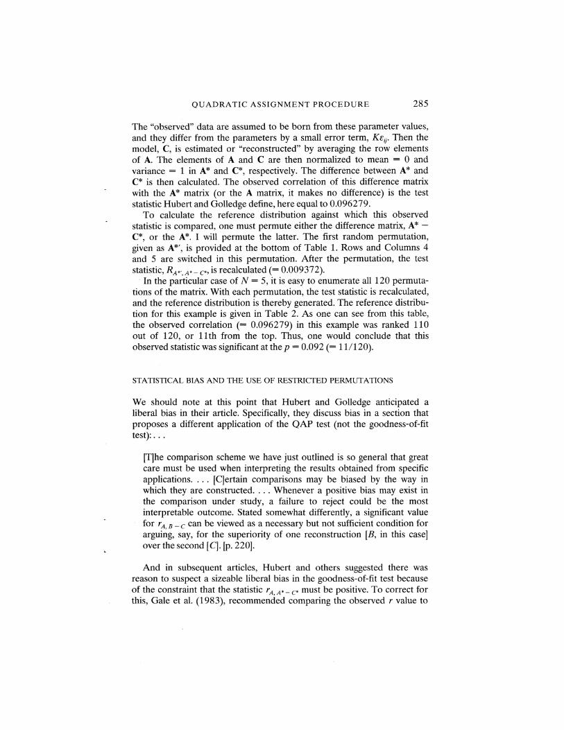
The "observed" data are assumed to be born from these parameter values, and they differ from the parameters by a small error term, Ktij· Then the model, C, is estimated or "reconstructed" by averaging the row elements of A. The elements of A and C are then normalized to mean = 0 and variance = 1 in A* and C*, respectively. The difference between A* and C* is then calculated. The observed correlation of this difference matrix with the A* matrix (or the A matrix, it makes no difference) is the test statistic Hubert and Golledge define, here equal to 0.096279.

To calculate the reference distribution against which this observed statistic is compared, one must permute either the difference matrix, A*­C*, or the A*. I will permute the latter. The first random permutation, given as A*', is provided at the bottom of Table 1. Rows and Columns 4 and 5 are switched in this permutation. After the permutation, the test statistic, RA*',A*- c•, is recalculated(= 0.009372).

In the particular case of N = 5, it is easy to enumerate all 120 permuta­tions of the matrix. With each permutation, the test statistic is recalculated, and the reference distribution is thereby generated. The reference distribu­tion for this example is given in Table 2. As one can see from this table, the observed correlation (= 0.096279) in this example was ranked 110 out of 120, or 11th from the top. Thus, one would conclude that this observed statistic was significant at the p = 0.092 (= 11/120).

STATISTICAL BIAS AND THE USE OF RESTRICTED PERMUTATIONS

We should note at this point that Hubert and Golledge anticipated a liberal bias in their article. Specifically, they discuss bias in a section that proposes a different application of the QAP test (not the goodness-of-fit test): ...

[T)he comparison scheme we have just outlined is so general that great care must be used when interpreting the results obtained from specific applications .... [C)ertain comparisons may be biased by the way in which they are constructed .... Whenever a positive bias may exist in the comparison under study, a failure to reject could be the most interpretable outcome. Stated somewhat differently, a significant value for rA 8 -c can be viewed as a necessary but not sufficient condition for arguiri.g, say, for the superiority of one reconstruction [B, in this case] over the second [C). [p. 220).

And in subsequent articles, Hubert and others suggested there was reason to suspect a sizeable liberal bias in the goodness-of-fit test because of the constraint that the statistic rA,A*- c• must be positive. To correct for this, Gale et al. (1983), recommended comparing the observed r value to

286 DAVID KRACKHARDT

TABLE II Rank order of test statistics based on 120 permutations (values rounded to the nearest ten

thousandths)

1 -0.1578 31 -0.0445 61 0.0050 91 0.0478 2 -0.1396 32 -0.0441 62 0.0050 92 0.0491 3 -0.1328 33 -0.0441 63 0.0053 93 0.0491 4 -0.1328 34 -0.0402 64 0.0053 94 0.0527 5 -0.1145 35 -0.0402 65 0.0068 95 0.0527 6 -0.1090 36 -0.0347 66 0.0068 96 0.0551 7 -0.1090 37 -0.0347 67 0.0090 97 0.0554 8 -0.1014 38 -0.0286 68 0.0090 98 0.0554 9 -0.0945 39 -0.0286 69 0.0094 99 0.0575

10 -0.0945 40 -0.0281 70 0.0131 100 0.0575 11 -0.0874 41 -0.0281 71 0.0131 101 0.0661 12 -0.0830 42 -0.0280 72 0.0171 102 0.0721 13 -0.0830 43 -0.0280 73 0.0171 103 0.0757 14 -0.0810 44 -0.0279 74 0.0180 104 0.0757 15 -0.0810 45 -0.0279 75 0.0181 105 0.0767 16 -0.0794 46 -0.0258 76 0.0181 106 0.0767 17 -0.0774 47 -0.0258 77 0.0222 107 0.0793 18 -0.0774 48 -0.0186 78 0.0258 108 0.0793 19 -0.0703 49 -0.0178 79 0.0272 109 0.0802 20 -0.0703 50 -0.0064 80 0.0272 110 0.0963 21 -0.0648 51 -0.0064 81 0.0281 111 0.1044 22 -0.0648 52 -0.0063 82 0.0281 112 0.1148 23 -0.0647 53 -0.0063 83 0.0302 113 0.1148 24 -0.0647 54 -0.0034 84 0.0302 114 0.1175 25 -0.0640 55 -0.0034 85 0.0305 115 0.1185 26 -0.0640 56 -0.0026 86 0.0347 116 0.1185 27 -0.0538 57 -0.0026 87 0.0347 117 0.1212 28 -0.0451 58 -0.0005 88 0.0437 118 0.1345 29 -0.0451 59 0.0043 89 0.0437 119 0.1459 30 -0.0445 60 0.0043 90 0.0478 120 0.1459

a restricted reference distribution composed of only permutations that generate positive values (Dow, 1985, also uses this procedure).

Referring back to the row-dominated model described in Tables 1 and 2, Gale et al. (1983) would adjust our prior conclusion about the signifi­cance level of the observed statistic. Instead of 120 permutations, we would only count the permutations that result in correlations greater than 0 in Table 2 as part of our reference distribution. One can see that there are 62 such permutations. Thus, our new significance level would be p =

0.177 (= 11/62) instead of the p = 0.092 calculated earlier. If we were using a prior alpha level of 0.10, then we would have concluded that the data were significantly different from the reconstructed model using the

QUADRATIC ASSIGNMENT PROCEDURE 287

unrestricted permutation test, but we would have concluded that the data were not significantly different from the model using the restricted per­mutation test, I note here that the unrestricted permutation test will necessarily result in a smaller p-value, and consequently the unrestricted test will always increase the chances that a sample data set will be found to be significantly different from the reconstruction, relative to the restricted test.

To see how these tests behave, I conducted Monte Carlo simulations of the exact procedure recommended by Hubert and Golledge. First, a "true" model of parameters is assumed. Second, "observed" data are generated by adding a small amount of error to the fixed parameter values. Third, the model parameters are estimated, or reconstructed, from the observed data. Fourth, the data are tested using the Hubert-Golledge test to deter­mine whether the observations are significantly different from the recon­structed estimates. If the Hubert-Golledge test has a reasonable proba­bilistic interpretation, then the probability of the test showing significant results at the alpha level should be approximately alpha.

I have generated two different types of models, one based on the row­dominated model described in Tables 1 and 2, and a second MDS model that precisely follows the suggested application in Hubert and Golledge discussed earlier. First, I will describe the simulation results of the row­dominated model.

ROW-DOMINATED MODEL RESULTS

The parameters in the M (fable 1) were fixed. Samples were generated by adding a known amount of error. The size of the error was determined by the size of K. K took on one of three relatively small values: 0.001, 0.01, and 0.1, so that in no case was the amount of error in the data overwhelm­ing. Additionally, I generated data using three different N-sizes, one with N = 5 (the one described in Table 1), one with N = 10, and one with N = 20. For each combination of N-size and K -weight, I generated 1000 samples (A in Table 1 ). For each sample, I tested the QAP statistic by permuting the matrix 1000 times for models based on N = 10 and N = 20; and for N = 5, the entire set of 120 permutations was used to test the statistic.

The performance of a statistical test should not depend on the particu­lar arbitrary alpha level chosen. If the data are generated in accordance with the tested model, then the test should reject the model alpha fraction of the time, regardless of what alpha is. Specifically, 5 percent of the samples should reject the model at the alpha= 0.05 level; 10 percent of the samples should reject the model at the alpha= 0.10 level, and so on. I performed tests for three alpha levels on each sample; alpha = 0.05,

288 DAVID KRACKHARDT

alpha= 0.10, and alpha = 0.20. Each test was based on both restricted and unrestricted permutations.

The results of these simulations are presented in Table 3. When K = 0.001 and N = 5, 187 of the 1000 samples were found to be significant using the unrestricted permutation test at the 0.05 level. Only 37 of the samples were found to be significant at the 0.05 level using the restricted permutation test. It is interesting to note that these proportions do not change dramatically as the amount of error increases for the N = 5 set. When K = 0.1, 165 of the samples are significant using the unrestricted permutation test, and 39 of the samples are significant using the restricted test.

While this insensitivity to error size may seem encouraging, it is mis­leading. This robustness does not reappear in samples where N = 10 or N = 20. More importantly, in none of the samples and under none of the tests does the probability of finding a significant result correspond to the alpha level chosen. When N = 5 and a criterion of 0.05 is used based on restricted permutations, the probability of finding a significant result is slightly less than alpha. When a criterion of 0.10 is used, the probability of finding a significant result is somewhat more than 0.10. In all other cases, the probability of a significant finding is far greater than alpha. Virtually all of the samples generated when K = 0.01 or greater and N = 10 or greater were significant at all three levels of alpha.

TABLE III Results of simulations of row-dominated model. Proportion of simulated samples that were

deemed significantly different from the reconstruction at the prescribed Alpha level

Alpha=0.05 Alpha=0.10 Alpha=0.20 Number of

K N u R u R u R Samples

0.001 5 0.187 0.037 0.592 0.168 0.982 0.549 1000 0.010 5 0.168 0.036 0.603 0.129 0.986 0.568 1000 0.100 5 0.165 0.039 0.647 0.167 0.991 0.614 1000

0.001 10 0.731 0.631 0.847 0.731 0.940 0.839 1000 0.010 10 0.999 0.930 1.000 1.000 1.000 1.000 1000 0.100 10 1.000 0.919 1.000 1.000 1.000 1.000 1000

0.001 20 0.653 0.614 0.682 0.651 0.729 0.686 1000 0.010 20 1.000 1.000 1.000 1.000 1.000 1.000 1000 0.100 20 1.000 1.000 1.000 1.000 1.000 1.000 1000

U =Unrestricted permutation tests R = Restricted permutation tests

QUADRATIC ASSIGNMENT PROCEDURE 289

MDS MODEL RESULTS

As mentioned earlier, Hubert and Golledge suggested that this test could be used to determine whether a particular n-dimensional MDS solution of a matrix of interpoint distances adequately accounts for the original data. The procedure to test the MDS solution is somewhat more complicated than that used to test the row-dominated model, but the underlying logic is very similar.

TABLE IV Example of calculations for simulation of MDS Model (N = 5, K = 0.001; value rounded

to the nearest thousandths)

Set of given (x, y) coordinates in model: 0.899 0.467 0.370 0.455 0.887 0.986 0.842 0.982 0.438 0.312

0.000 0.529 0.519 0.517 0.486 Matrix of pairwise 0.529 0.000 0.741 0.707 0.158 Euclidean distances

M= 0.519 0.741 0.000 0.045 0.810 in model 0.517 0.707 0.045 0.000 0.782 0.486 0.158 0.810 0.782 0.000

0.000 0.530 0.520 0.517 0.486 "Observed" 0.530 0.000 0.742 0.707 0.158 pairwise distances

A= 0.520 0.742 0.000 0.044 0.809 (=model+ error) 0.517 0.707 0.044 0.000 0.784 0.486 0.158 0.809 0.784 0.000

Set of (x, y) coordinates obtained from MDS program on negative of A (Stress > 0.01)

0.209 -0.849 0.741 0.797

-1.069 0.259 -0.890 0.038

1.009 -0.169

0.000 1.731 1.692 1.366 1.050 Reconstruction 1.731 0.000 1.889 1.833 1.003 matrix of pairwise

C= 1.692 1.889 0.000 0.348 2.121 Euclidean distances 1.366 1.833 0.348 0.000 0.903 calculated from 1.050 1.003 2.121 1.903 0.000 MDS solution above

0.000 0.003 -0.040 -0.052 -0.179 Normalized 0.003 0.000 0.868 0.728 -1.523 "observed" data

A*= -0.040 0.868 0.000 -1.991 1.146 -0.052 0.728 -1.991 0.000 1.040 -0.179 -1.523 1.146 1.040 0.000

290 DAVID KRACKHARDT

Table IV (Continued)

0.000 0.457 0.382 -0.246 -0.854 Normalized 0.457 0.000 0.762 0.653 -0.945 reconstruction

C*= 0.382 0.762 0.000 -2.207 1.210 -0.246 0.653 -2.207 0.000 0.788 -0.854 -0.945 1.210 0.788 0.000

0.000 -0.454 -0.422 0.194 0.674 Difference in -0.454 0.000 0.107 O.D75 -0.578 normalized

A*-C*= -0.422 0.107 0.000 0.216 -0.063 matrices 0.194 O.Q75 0.216 0.000 0.252 0.674 -0.578 -0.063 0.252 0.000

Observed r = 0.1831952

First permutation of A* 0.000 -1.991 1.146 0.868 -0.040 A sample

-1.991 0.000 1.040 0.728 -0.052 permutation A*'= 1.146 1.040 0.000 -1.523 -0.179 of A*

0.868 0.728 -1.523 0.000 0.003 -0.040 -0.052 -0.179 0.003 0.000

rA'',A'- C' = 0.1203248

Table 4 provides a step-by-step account of the Hubert-Golledge proce­dure. First, I assume a "true" two-dimensional model of (x, y) coordinates. From these coordinates, I calculate the exact interpoint distances of all pairs of points. This represents the "true" interpoint distances (= M). I add a small amount of error to these distances to create the "observed" matrix of distances A. I then estimate or reconstruct the two-dimensional model from which A was generated by multiplying A by the scalar -1 (to turn A into a similarity matrix) and running it through an MDS program, extracting the (x, y) coordinates. Note that the stress for this solution is very low (less than 0.01), which is no surprise since only a small amount of error was added to the "true" distances. I then estimate or reconstruct M by calculating the Euclidean distances among the five points (= C). Both A and C are normalized to mean = 0 and variance = 1 and called A* and C*, respectively. The difference between them is calculated, and the correlation between A* and A* - C* is computed as the test statistic.

To create the reference distribution, A* was permuted 1000 times, and the test statistic rA*' A*- C* was recalculated each time. The first permuta­tion is provided at the bottom of Table 4. The rows and columns (1, 2, 3, 4, 5) were reordered as (5, 4, 1, 2, 3) in A*'.

Again, I varied theN-size of the matrix and the error weight K to see if the test was sensitive to those parameters (see Table 5). For each of

QUADRATIC ASSIGNMENT PROCEDURE 291

the nine models, 1000 samples were drawn and tested using both the restricted and unrestricted permutation tests at the 0.05, 0.10, and 0.20 alpha levels.

TABLE V Results of simulations of MDS model. Proportion of simulated samples that were deemed

significantly different from the reconstruction at the prescribed Alpha level

Alpha=0.05 Alpha=0.10 Alpha=0.20 Number of

K N u R u R u R Samples

0.001 5 0.000 0.000 0.000 0.000 0.000 0.000 1000 0.010 5 0.000 0.000 0.002 0.000 0.008 0.001 1000 0.100 5 0.018 0.006 0.037 0.014 0.129 0.034 1000

0.001 10 0.000 0.000 0.000 0.000 0.000 0.000 1000 0.010 10 0.000 0.000 0.000 0.000 0.000 0.000 1000 0.100 10 0.013 0.000 0.218 0.012 0.919 0.191 1000

0.001 20 0.000 0.000 0.000 0.000 0.000 0.000 1000 0.010 20 0.002 0.000 0.002 0.002 0.002 0.002 1000 0.100 20 1.000 0.967 1.000 0.999 1.000 1.000 1000

U =Unrestricted permutation tests R = Restricted permutation tests

The results in this simulation are even less encouraging than in the row­dominated model simulation. When N = 5, all of the tests for each of the error weights were far less than the prescribed alpha levels. When N = 10, only in the case where 1) the prescribed alpha was 0.20, 2) the error weight 0.1, and 3) the restricted permutation test was used, did the probability (= 0.191) of a significant finding approach alpha. When N = 20, the results are very unstable, with the probability of a significant finding being either very close to 0 or very close to 1 under all conditions.

DISCUSSION

In summary, in neither the row-dominated model nor in the MDS model did the test perform in accordance with the statistical interpretation of the test. In the row-dominated model, the QAP test of fit was largely too liberal, although not universally. In the MDS model, the results were either vastly too liberal or too conservative, depending on the N-size and the precise size of the small amount of error added.

Recall that Hubert and Golledge anticipated a possible positive or

292 DAVID KRACKHARDT

liberal bias in the way these tests are constructed, suggesting that a signifi­cant finding "can be viewed as a necessary but not sufficient condition" for drawing the appropriate statistical conclusion. The results of the simula­tions reported in this paper suggest that an insignificant p-value is neither necessary nor sufficient for concluding that the data are "adequately reconstructed." Because the test is sometimes too liberal, in cases where the data are disproportionately found to be significantly different from the reconstruction, one cannot claim that an insignificant result constitutes a necessary condition for concluding that the data are adequately recon­structed. Conversely, because the test is sometimes too conservative, in cases where the data are disproportionately found to be not significantly different from the reconstruction, one cannot claim that an insignificant result constitutes a sufficient condition for concluding that the data are adequately reconstructed. In short, an insignificant rA*,A*- c• does not imply that the data are adequately reconstructed, nor does a significant r A •, A._ C* imply that the data are not adequately reconstructed.

PERMUTATION TESTS AND PARAMETRIC SIMULATIONS

The QAP test is a permutation test, a member of a family of conditional statistical tests. The QAP test was designed for cases where parametric assumptions about the data are unknown. Hubert and Golledge are careful not to refer to a population from which the observations are sampled. In fact, no population is assumed; rather the data are assumed to comprise the population and hence no assumptions about sampling from a popula­tion are necessary.

On the other hand, the models I have used to test the behavior of this test are stochastic, parametric, non-conditional models. One might argue that my simulations have not truly tested the kinds of models the QAP test was designed for, since my parametric models are not conditional models.

The argument is insufficient. The reason for using conditional tests is that it does not require assumptions about the error terms in the popula­tion. When parametric assumptions are untenable, the nonparametric tests are used because they are not dependent on such assumptions. Thus, the nonparametric tests are more general; they apply to situations in which the parametric tests may not apply. Simply because the nonparametric test is applicable to a wider range of population characteristics and assumptions than the parametric case does not mean that the nonparametric test is inapplicable if one happens to know the parametric nature of the popula­tion. A more general test must certainly work in a specific case. It seems to me that a minimal criterion for the adequacy of a nonparametric test is that it should behave appropriately in a well-defined parametric case.

QUADRATIC ASSIGNMENT PROCEDURE 293

INTERPRETING rA*,A*- C'

What does the probability associated with the QAP test of fit mean? How might it be reasonably interpreted? I have argued that it is not the proba­bility of observing this test statistic value given a null hypothesis that p =

0, as demonstrated logically earlier. And the simulations demonstrate that it dearly is not the probability of observing the statistic value given a model and assuming the observations are born from the model with a little error added.

If I were to give the Hubert-Golledge fit statistic an interpretation, I would say it was descriptive, not inferential. For example, R-square is a perfectly good measure of fit; and R-square of 0.8 is a better fit than an R-square of 0.2. If the p-value derived from the QAP test of fit is 0.1, I might be able to say, all else being equal, that the reconstruction is a better fit than if the p-value had been 0.01. I would never ascribe an inferential or probabilistic interpretation to my R-square measure. Similarly, I cannot ascribe a reasonable inferential or probabilistic interpretation to my QAP test results.

CONCLUDING REMARKS

This paper has attempted to focus attention on the problem of using QAP to test whether data are fit well by a particular reconstruction. It was shown logically that the underlying null hypothesis in the QAP test is not reasonable. Moreover, the simulations demonstrate that the QAP good­ness-of-fit test is inappropriate as a statistical test to the class of models that Hubert and Golledge recommended.

In statistical terms, parametric tests of goodness-of-fit are well defined. They stipulate both a set of parameters and error distributions around those parameter values. The non-parametric QAP permutation procedure never asks the question how are the observations likely to be distributed around the population parameters. If one has no idea how the outcomes are distributed, one has little hope of answering a question about the probability of observing any particular outcome.

In conclusion, I would like to emphasize the point that QAP has opened up possibilities for the testing of hypotheses that were previously untestable. Much has been written about the distribution of r (or the raw cross-product index) under various conditions (Dietz, 1983; Mielke, 1978; 1979; Faust and Romney, 1985; Krackhardt, 1988; 1991; Romney and Weller, 1989). More attention should be place on the conditions under which a permutation model is reasonable or interpretable, given the structure of the data. This paper hopes to make a start in that direction.

294 DAVID KRACKHARDT

ACKNOWLEDGEMENTS

This paper grew from work jointly conducted with Ronald L. Brieger on the application of QAP to loglinear problems (Krackhardt and Brieger, 1985). In addition, I would like to thank Larry Hubert and Charles McCulloch. Their comments and encouragement on earlier versions of this manuscript were most helpful.

REFERENCES

Baker, F. B. and L. J. Hubert, 1981 The Analysis of Social Interaction Data. Sociological Methods and Research 9:339-361.

Dietz, E. J., 1983 Permutation Tests for Association Between Two Distance Matrices. Systematic Zoology 32:21-26.

Douglas, M. E. and J. Endler, 1982 Quantitative Matrix Comparisons in Ecological and Evolutionary Investigations. Journal of Theoretical Biology 99:777-795.

Dow, M. and J. Cheverud, 1985 Comparison of Distance Matrices in Studies of Population Structure and Genetic Micro Differentiation: Quadratic Assignment. American Journal of Physical Anthropology, 68: 367-373.

Dow, M., 1985 Nonparametric Inference Procedures for Multistate Life Table Analysis. Journal of Mathematical Sociology, 11: 245-263.

Faust, K. and A. K. Romney, 1985 The Effect of Skewed Distributions on Matrix Permutation Tests. British Journal of Mathematical and Statistical Psychology, 38: 152-160.

GaleN., L. J., Hubert, W. R., Tobler and R. G., Golledge, 1983 Combinatorial Procedures for the Analysis of Alternative Models: An Example from Interregional Migration. Papers of the Regional Science Association, 53: 105-115.

Hubert, L. J. 1987 Assignment Methods in Combinatorial Data Analysis. New York: Marcel Dekker.

Hubert, L. J. and R. G. Golledge, 1981 A Heuristic Method for the Comparison of Related Structures. Journal of Mathematical Psychology, 23: 214-226.

Hubert, L. J., R. G. Golledge, and C. M. Costanzo, 1981 Generalized Procedures for Evaluating Spatial Autocorrelation. Geographical Analysis, 13: 224-233.

Hubert, L. J. and J. Schultz, 1976 Quadratic Assignment as a General Data Analysis Strategy. British Journal of Mathematical and Statistical Psychology, 29: 190-241.

Krackhardt, D. (February, 1991) Multiple Regression QAP: Analytic vs. Permutation Methods. Unpublished Manuscript.

Krackhardt, D. and M. Kilduff, 1990 Friendship Patterns and Culture: The Control of Organizational Diversity. American Anthropologist, 92: 142-154.

Krackhardt, D. 1987 QAP Partialling as a Test of Spuriousness. Social Networks, 9: 171-186.

Krackhardt, D. 1988 Predicting with Networks: A Multiple Regression Approach to Analyzing Dyadic Data. Social Networks, December 10(4): 359-381.

Krackhardt, D. and R. Brieger, 1985 Comparative Advantages of QAP Partialling and Log Linear Analysis of Multivariate Network Data. Paper Given at Fifth Annual Social Network Conference, Palm Beach, Florida.

Krackhardt, D. and L. W. Porter, 1986 The Snowball Effect: Turnover Embedded in Communication Networks. Journal of Applied Psychology, 71:50-5 5.

QUADRATIC ASSIGNMENT PROCEDURE 295

Laumann, E. 0. and F. U. Pappi, 1976 Networks of Collective Action: A Perspective on Community Influence Systems. New York: Academic Press.

Mantel, N. 1967 The Detection of Disease Clustering and a Generalized Regression Approach. Cancer Research, 27: 209-220.

Mielke, P. W. 1979 On Asymptotic Non-Normality of Null Distributions of MRPP Statistics. Communications in Statistics -Theory and Methods, 8: 1541-15 50.

Mielke, P. W. 1978 Clarification and Appropriate Inferences for Mantel and Valand's Nonparametric Multivariate Analysis Technique. Biometrics, 34: 277-282.

Morrison, D. E. and R. E. Henkel, (Eds.). 1970 The Significance Test Controversy. Chicago: Airline. ·

Nakao, K. and A. K. Romney, 1984 A Method for Testing Alternative Theories: An Example from English Kinship. American Anthropologist, 86: 668-673.

Romney, A. K. and S. C. Weller, 1989 Systemic Culture Patterns and High Concordance Codes. In Ralph Bolton (Ed.), The Content of Culture: Constants and Variants. New Haven: HRAF Press, 363-381.

Sokal, R. R. 1979 Testing Statistical Significance of Geographic Variation Patterns. Systematic Zoology, 28: 227-232.

APPENDIX:

~ ProofofrA,A*-c•= ~ ~

1. By construction:

A-X C-Xc A*= A C* = __ ____::__ SDA SDc

Therefore, XA. = Xc• = 0 and Var(A*) = Var(C*) = 1

Cov(A*, A*- C*) 2· rA*,A*- c• = Jvar(A*) Var(A*- C*)

Cov(A*, A*- C*) = Var(A*)- Cov(A*, C*)

= 1- Cov(A*, C*)

Var(A*- C*) = Var(A*) + Var(C*)- 2 Cov(A*, C*)

= 2-2 Cov(A*, C*)

rA*,A*- c•

= 2(1- Cov(A*, C*)

1- Cov(A*, C*)

J2(1- Cov(A*, C*))

1- Cov(A*, C*)

2

296 DAVID KRACKHARDT

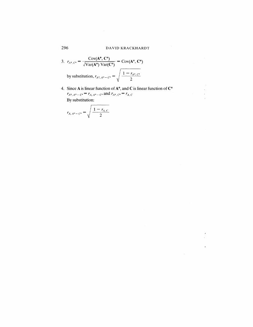
3. rA*, C* = Cov(A*, C*) = Cov A* C* Jvar(A*) Var(C*) ( ' )

. . ~ bysubstltutton, rA*,A*-C* = ~ ~

4. Since A is linear function of A*, and Cis linear function of C* rA*,A*- C* = rA,A*- C* and rA*, C* = rA, C

By substitution:

~ rA,A*- C* = ~ ~