A case study of boundary layer ventilation by convection...

A case study of boundary layer ventilation by convection and coastal processes Article

Published Version

Dacre, H. F., Gray, S. L. and Belcher, S. E. (2007) A case study of boundary layer ventilation by convection and coastal processes. Journal of Geophysical Research, 112 (D17). D17106. ISSN 01480227 doi: https://doi.org/10.1029/2006JD007984 Available at http://centaur.reading.ac.uk/880/

It is advisable to refer to the publisher’s version if you intend to cite from the work. Published version at: http://www.agu.org/pubs/crossref/2007/2006JD007984.shtml

To link to this article DOI: http://dx.doi.org/10.1029/2006JD007984

Publisher: American Geophysical Union

All outputs in CentAUR are protected by Intellectual Property Rights law, including copyright law. Copyright and IPR is retained by the creators or other copyright holders. Terms and conditions for use of this material are defined in the End User Agreement .

www.reading.ac.uk/centaur

CentAUR

http://centaur.reading.ac.uk/licence

http://www.reading.ac.uk/centaur

Central Archive at the University of Reading

Reading’s research outputs online

A case study of boundary layer ventilation by

convection and coastal processes

H. F. Dacre,1 S. L. Gray,1 and S. E. Belcher1

Received 31 August 2006; revised 23 February 2007; accepted 4 June 2007; published 12 September 2007.

[1] It is often assumed that ventilation of the atmospheric boundary layer is weak inthe absence of fronts, but is this always true? In this paper we investigate the processesresponsible for ventilation of the atmospheric boundary layer during a nonfrontal day thatoccurred on 9 May 2005 using the UK Met Office Unified Model. Pollution sources arerepresented by the constant emission of a passive tracer everywhere over land. Theventilation processes observed include shallow convection, turbulent mixing followed bylarge-scale ascent, a sea breeze circulation and coastal outflow. Vertical distributions oftracer are validated qualitatively with AMPEP (Aircraft Measurement of chemicalProcessing Export fluxes of Pollutants over the UK) CO aircraft measurements and areshown to agree impressively well. Budget calculations of tracers are performed in order todetermine the relative importance of these ventilation processes. Coastal outflow and thesea breeze circulation were found to ventilate 26% of the boundary layer tracer by sunsetof which 2% was above 2 km. A combination of coastal outflow, the sea breezecirculation, turbulent mixing and large-scale ascent ventilated 46% of the boundary layertracer, of which 10% was above 2 km. Finally, coastal outflow, the sea breezecirculation, turbulent mixing, large-scale ascent and shallow convection togetherventilated 52% of the tracer into the free troposphere, of which 26% was above 2 km.Hence this study shows that significant ventilation of the boundary layer can occur in theabsence of fronts (and thus during high-pressure events). Turbulent mixing and convectionprocesses can double the amount of pollution ventilated from the boundary layer.

Citation: Dacre, H. F., S. L. Gray, and S. E. Belcher (2007), A case study of boundary layer ventilation by convection and coastal

processes, J. Geophys. Res., 112, D17106, doi:10.1029/2006JD007984.

1. Introduction

[2] Much of the pollution in the atmosphere originatesfrom emissions in the atmospheric boundary layer, theregion of the atmosphere closest to the Earth’s surfacewhere the properties of air parcels are strongly modifiedby the presence of the Earth’s surface. The depth of thislayer is variable, changing with location, time of day andmeteorological situation. A stable layer at the top of theboundary layer often separates boundary layer air from airthat is not affected by the Earth’s surface, known as the freetroposphere. This stable layer can inhibit the transport of airfrom the boundary layer to the free troposphere. In theboundary layer we often observe lower wind speeds than inthe free troposphere and a different wind direction due tosurface friction. Thus if pollution remains trapped within theboundary layer it typically does not travel far and can buildup to become a local air pollution problem. In the freetroposphere there is no dry deposition to the surface andmost rates of chemical transformation are lower because

of colder temperatures. Colder temperatures can enhancesolubility and hence wet deposition of pollutants [Hobbs,2000] but typically pollutants in the free troposphere havelonger lifetimes than in the boundary layer. Thus if pollu-tants are transported to the free troposphere from theboundary layer, the longer lifetimes and higher wind speedsmay greatly expand their range of influence and the local airpollution problem can become a regional or even a globalproblem. Therefore boundary layer ventilation is a keyprocess in linking local air quality and global climatechange.[3] To explain the distribution of chemical species in the

free troposphere it is important to understand boththe chemistry and the dynamical processes responsible forthe transport of pollution. Observational and modelingstudies have shown that a wide range of processes may beimportant for boundary layer ventilation.[4] 1. Advective processes include transport by the warm

and cold conveyor belts associated with frontal systems[Kowol-Santen et al., 2001; Donnell et al., 2001; Esler et al.,2003; Agustı-Panareda et al., 2005], sea breeze circulationsand coastal outflow [Lu and Turco, 1994; Leon et al., 2001;Angevine et al., 2006; Verma et al., 2006] and mountainventing [Lu and Turco, 1994; Baltensperger et al., 1997;Seibert et al., 1998; Kossmann et al., 1999].

JOURNAL OF GEOPHYSICAL RESEARCH, VOL. 112, D17106, doi:10.1029/2006JD007984, 2007ClickHere

for

FullArticle

1Department of Meteorology, University of Reading, Reading, UK.

Copyright 2007 by the American Geophysical Union.0148-0227/07/2006JD007984$09.00

D17106 1 of 18

http://dx.doi.org/10.1029/2006JD007984

[5] 2. Mixing processes include deep convection[Dickerson et al., 1987; Lu and Turco, 1994; Hauf et al.,1995; Wang and Prinn, 2000], shallow convection [Flatøyand Hov, 1995; Edy et al., 1996; Gimson, 1997], frontalconvection [Esler et al., 2003; Agustı-Panareda et al.,2005], and boundary layer turbulence [Angevine et al.,2006; Verma et al., 2006].[6] The relative importance of these transport mecha-

nisms is not well known and is likely to depend on thesynoptic situation under consideration.[7] It is often assumed that there is little ventilation of

the atmospheric boundary layer into the free troposphereduring nonfrontal days, so that pollutant levels simply buildup in the boundary layer. This is probably a good assump-tion on days on which there is no observed convection.Nevertheless, shallow convection is a common featureduring nonfrontal days over Europe in the summer.[8] In this paper we concentrate on the transport processes

that occur during a nonfrontal day. A high-pressure regionwas situated to the west of the UK on this day. The event wassimulated using the UK Met Office nonhydrostatic UnifiedModel. This case study was chosen because we are interestedin ventilation of pollution in the absence of fronts and on dayscharacterized by widespread shallow convection. This willprovide insight into ventilation mechanisms that can occuron high-pressure days. Also, this case occurred duringthe Aircraft Measurement of chemical Processing Exportfluxes of Pollutants over the UK (AMPEP) field campaignon which measurements of pollution were carried out (http://badc.nerc.ac.uk/data/polluted-tropo/projects/ampep.html).This allows us to qualitatively compare results from themodel with observations. We aim to address two questions.First, can a mesoscale model simulate pollution transport ina manner consistent with the observations? This questionneeds to be addressed to determine which ventilationprocesses are realistically represented by the model. Second,by what ventilation processes does polluted boundary layerair enter the free troposphere in the absence of fronts, andwhat are their relative importance?[9] Nonfrontal processes for boundary layer ventilation

are described in section 2. The model used in this paper isdescribed briefly in section 3. In section 4 an overview ofthe case study is given. The numerical experiments havebeen performed using the UK Met Office Unified Modelwith passive tracers. The experimental details are describedin section 5. The results from numerical experiments for thecase study are described in section 6 and they are comparedwith observations from the AMPEP field campaign insection 7. Tracer budgets are calculated in section 8. Finally,in section 9 the main conclusions are given.

2. Processes for Boundary Layer VentilationDuring Nonfrontal Days

[10] Here we briefly review previous research which hasconsidered boundary layer ventilation by convection andsea breezes. These are the processes that could lead totransport during nonfrontal days. Ventilation by warm andcold conveyor belts is associated with frontal events andmountain venting is not significant over the UK. Hencethese mechanisms are not discussed further here.

[11] Chatfield and Crutzen [1984] hypothesized thatconvective transport is a major redistributor of pollutantsfrom the boundary layer to the free atmosphere. Rapidupdraughts are effective in ventilating the boundary layerand raising pollutants through many kilometers in tensof minutes. Evaporatively cooled downdraughts can beeffective in bringing pollution from the free atmosphereinto the boundary layer. Boundary layer turbulence maythen be an important process in bringing the pollutantsdown to the ground. There have been several studiesinvestigating transport of pollution by deep (>10 km)convective thunderstorms, Dickerson et al. [1987], Haufet al. [1995], Wang and Prinn [2000] and Lu et al. [2000].Nevertheless, over the UK, such deep convection is rarecompared to shallow (<5 km) convection. Daytime shallowcumulus clouds are common over the UK during thesummer and so, even though shallow convection inducesweaker vertical transport than deep convection, they cancontribute to nonnegligible amounts of pollution transport.Thompson et al. [1994] constructed a regional budget forboundary layer CO over the central US for June. Theycalculated horizontal fluxes into and out of the boundarylayer, surface fluxes due to anthropogenic emissions, bio-genic sources and deposition, photochemical productionand loss of CO, and vertical fluxes due to deep convection.They assumed that the budget residual was due to ventila-tion of the boundary layer by shallow cumulus clouds andsynoptic-scale frontal weather systems. This residual wasestimated to be about the same magnitude as the net COflux due to deep convection. Although they did not calcu-late the CO fluxes due to shallow convection and synoptic-scale weather systems explicitly, their study suggests theimportance of these processes.[12] There have been a few studies carried out to inves-

tigate the transport of pollution by shallow convection.Flatøy and Hov [1995] in their 3-D Mesoscale ChemistryTransport model found that during a 10-day period, char-acterized by high pressure and frequent occurrencesof cumulus convection over Europe, that convection dom-inates over the synoptic-scale vertical advection as aventilation mechanism. Their continental study has a hori-zontal resolution of 150 km and coarse vertical resolution inthe lower troposphere so it may not represent the ventilationof the boundary layer by convective and boundary layerturbulent mixing processes well. Edy et al. [1996] modeledCO redistribution by shallow convection over the Amazo-nian rain forest using a 2-D convective cloud model coupledwith a chemical model. They showed that 40% of thepollution emitted below 500 m reached 2000 m in altitude.However, this simulation modeled the evolution of a singleconvective cloud over a period of 2 hours. It is not clearwhether these results can be scaled up to represent theventilation of the boundary layer by widespread shallowconvection over an entire day. Gimson [1997] modeledpollution transport by shallow convective clouds in the airbehind a cold front using the UK Met Office Unified Model.Tracer was emitted 500 m above the surface and was trans-ported to upper levels by shallow convection with a localmaxima found at cloud top level (4–5 km). Comparisonswith large eddy model simulations were made but nocomparison with observations were carried out.

D17106 DACRE ET AL.: BOUNDARY LAYER VENTILATION PROCESSES

2 of 18

D17106

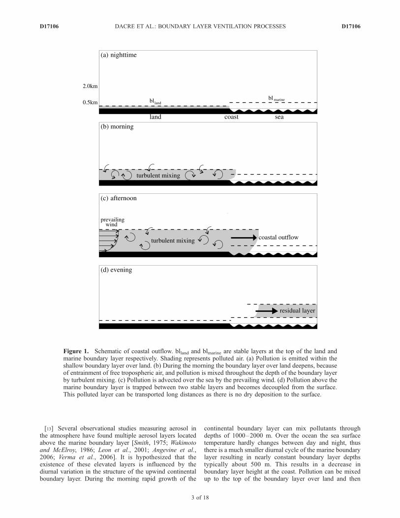
[13] Several observational studies measuring aerosol inthe atmosphere have found multiple aerosol layers locatedabove the marine boundary layer [Smith, 1975; Wakimotoand McElroy, 1986; Leon et al., 2001; Angevine et al.,2006; Verma et al., 2006]. It is hypothesized that theexistence of these elevated layers is influenced by thediurnal variation in the structure of the upwind continentalboundary layer. During the morning rapid growth of the

continental boundary layer can mix pollutants throughdepths of 1000–2000 m. Over the ocean the sea surfacetemperature hardly changes between day and night, thusthere is a much smaller diurnal cycle of the marine boundarylayer resulting in nearly constant boundary layer depthstypically about 500 m. This results in a decrease inboundary layer height at the coast. Pollution can be mixedup to the top of the boundary layer over land and then

Figure 1. Schematic of coastal outflow. blland and blmarine are stable layers at the top of the land andmarine boundary layer respectively. Shading represents polluted air. (a) Pollution is emitted within theshallow boundary layer over land. (b) During the morning the boundary layer over land deepens, becauseof entrainment of free tropospheric air, and pollution is mixed throughout the depth of the boundary layerby turbulent mixing. (c) Pollution is advected over the sea by the prevailing wind. (d) Pollution above themarine boundary layer is trapped between two stable layers and becomes decoupled from the surface.This polluted layer can be transported long distances as there is no dry deposition to the surface.


3 of 18

D17106

advected horizontally above the marine boundary layer. Weterm this process ‘‘coastal outflow’’ here (defined at the endof this section). Differential heating between the land andthe sea also leads to the formation of a sea breeze. Collisionbetween a sea breeze and the prevailing wind can result inpolluted air being transported away from the Earth’s surface.Further advection of this pollution across the coastlineresults in its ventilation from the boundary layer.[14] A few studies have investigated the ventilation of

pollution along the coast. Schultz and Warner [1982] carriedout two-dimensional idealized simulations of pollutionventilation in the Los Angeles Basin. They found thatfor calm synoptic-scale wind conditions, sea breeze andmountain circulations dominated the ventilation. Ventilationwas greatest in the vicinity of the sea breeze front. Leonet al. [2001] observed a layer of aerosol above the NorthIndian Ocean marine boundary layer. Their mesoscale

modeling study showed that convergence between the seabreeze and the northeast monsoon winds along the westcoast of India can transport air up to 2.5 km in altitude overland. However, the katabatic winds associated with the steeporography in this region may enhance the sea breezecirculation making it difficult to isolate the sea breeze asa ventilation process. Lu and Turco [1994] carried outidealized 2-D modeling of sea breeze and mountain venti-lation and found that sea breezes as well as upslope windsboth create vertical transport that can lead to the formationof elevated pollution layers. When mountains are close tothe coastline, the sea breeze and mountain flows arestrongly coupled.[15] In this paper the term coastal outflow is used to

describe the decoupling of pollution from the surface via theformation of an internal stable boundary layer which occurswhen there is horizontal transport from land to sea and the

Figure 2. UK Met Office surface pressure analysis at 0000 UTC on 9 May 2005.

Figure 3. Tephigram from 1200 UTC 9 May 2005Waddington RAF (53�N, 0�W, shown on Figure 5a).

Figure 4. Visible image of the UK from the Modis Aquasatellite at 1245 UTC on 9 May 2005. Courtesy of NASAGoddard Space Flight Center.


4 of 18

D17106

land boundary layer is deeper than the marine boundarylayer (as is typically the case on summer days, see Figure 1).Ventilation is used loosely to encompass any processleading to the decoupling of pollutants from the surface.Thus we include coastal outflow in this definition althoughit is not strictly a venting process.[16] We have chosen a case study in which widespread

shallow convection occurs over the UK. We aim to simulatethe ventilation of pollution by shallow convection, the seabreeze circulation and coastal outflow and compare ourmodel results with AMPEP aircraft observations.

3. UK Met Office Unified Model

[17] The case has been simulated using the UK MetOffice Unified Model version 5.5. This is an operationalforecast model that contains leading edge physics anddynamics. The model is a nonhydrostatic primitive equationmodel using a semi-implicit, semi-Lagrangian numericalscheme [Cullen, 1993]. The model includes a comprehensiveset of parameterizations, including boundary layer [Locket al., 2000], mixed phase cloud microphysics [Wilson andBallard, 1999] and convection [Gregory and Rowntree,1990]. There is no explicit diffusion in the model. A limitedarea domain with horizontal resolution 0.11� (approx12.5 km) was used over Europe extending from 44�N to64�N latitude and 12�W to 16�E longitude. The model has38 levels in the vertical on a stretched grid ranging from thesurface to 5 hPa. This corresponds to approximately 100 mlayer spacing in the boundary layer and 500 m layerspacing in the midtroposphere. The first tracer model levelis at 20 m.[18] The boundary layer in the model is defined by the

number of turbulent mixing levels (NTML). For stableconditions this is the region in contact with the surfacewhere the bulk Richardson number is smaller than 1. Forunstable conditions an adiabatic moist parcel ascent is

performed in the model; ascent is stopped when the parcelbecomes negatively buoyant. If the layer is well mixed theNTML is set to the parcel ascent top (inversion height). Ifthe layer is cumulus capped the NTML is set to the liftingcondensation level (cloud base). Thus the NTML is a goodrepresentation of the boundary layer, defined as the layerwhere mixing down to the surface is possible over shorttimescales.

4. Overview of the Case Study

[19] Figure 2 shows the UK Met Office surface pressureanalysis for 0000 UTC on 9 May 2005. A high-pressureregion approached the UK from the west becoming centeredover the UK at 2100 UTC on 10 May. Figure 3 shows atephigram for 1200 UTC on 9 May 2005 launched atWaddington (53�N, 0�W). There are weak northerly windsnear the surface and stronger northwesterly winds above2 km. There is also evidence of layers of increased staticstability at 1000 m and at 3500 m. Figure 4 shows a visibleimage from the Modis Aqua satellite at 1245 UTC on 9 May2005. Surface heating led to the outbreak of widespreadshallow convection over the whole of the UK on this day.

5. Tracer Experiments

[20] Tracer sources are represented in the model by aconstant emission of tracer everywhere over land at a rate of5 � 10�7 kgm�2s�1 emitted 20 m above the surface.(Tracers are also initialized everywhere within the boundarylayer (uniform concentration 1 � 10�7 kg/kg for all tracers).However the source emissions rapidly swamp the initialconditions.) Although the numerical experiments are aimedat identifying processes, the value of emission rate is chosento mimic CO emissions. Uniform emissions were used toenable the relative importance of the different mechanismsto be determined. Realistic emissions would enable quanti-tative comparison with observations. However, the interpre-

Figure 5. Tracer in the free troposphere integrated over height, contours every 0.03 kg/m2 at(a) 1300 UTC and (b) 1700 UTC. Tracer is transported by advection only. Solid line indicates verticalcross section shown in Figures 6, 10, 13 and 15. Boxes indicate domain used in Figure 20c.


5 of 18

D17106

tation of the results would be significantly complicated ifthe colocation of strong emission sources and localizedventilation mechanisms (such as convection and the seabreeze circulation) had to be considered.[21] Four separate tracers have been used which are

transported by different combinations of transport schemes,namely, the advection, convection and turbulent mixingschemes. The tracers in our simulation are treated as passivesubstances, meaning that they are subject to advection,convection and turbulent mixing but are neither depositednor chemically transforming. This methodology, in whichseparate tracers transported by the schemes are used toattribute transport to different mechanisms, has also been

used by Donnell et al. [2001], Gray [2003] and Agustı-Panareda et al. [2005].

6. Model Results

[22] First, the transport of the tracer which is advectedonly is described, second, the tracer that undergoes advec-tion and turbulent mixing is described and finally, the tracerthat undergoes advection, turbulent mixing and convectionis described.

6.1. Advection Only

[23] Figure 5 shows the tracer in the free troposphereintegrated over height for the case in which the tracer is

Figure 6. Vertical cross sections of potential temperature (solid). Bold contours indicate the q contoursthat follow levels of increased static stability (not shown) overlaid with NTML (dashed) at (a) 0900 UTC,(b) 1300 UTC and (c) 1700 UTC.


6 of 18

D17106

transported by advection only. The free troposphere isdefined as being above the top of the boundary layer(defined by NTML, see section 3). There is no freetropospheric tracer at the start of the forecast as tracer isemitted 20 m above the surface. By 1300 UTC, Figure 5a,there is still very little tracer in the free troposphere.However, by 1700 UTC, Figure 5b, tracer is found in thefree troposphere mainly located along the south coasts ofEngland, Ireland and Wales.[24] To determine the advective mechanism responsible

for this boundary layer ventilation, vertical cross sectionswere taken along the line shown in Figure 5a. Vertical crosssections of potential temperature, q, are shown in Figure 6.Contours of q that approximately follow layers of increasedstatic stability (not shown) have been plotted in bold. At0900 UTC, Figure 6a, a well mixed layer extends from thesurface to 750 m over land and from the surface to 500 mover the sea. A weak stable layer separates the well mixedboundary layer air from free tropospheric air above. Thestable layer over land is indicated by the bold q = 281 Kcontour, and over the sea by the bold q = 280 K contour. Inthe free atmosphere there is a strong stable layer indicatedby the bold q = 289 K contour which slopes from 3500 mover land to 2750 m over the sea. By 1300 UTC, Figure 6b,turbulent mixing over land has led to an increase in theheight of the boundary layer up to 1300 m. The stable layers

over land at the top of the boundary layer (1300 m) andin the free troposphere (3500 m) are consistent withthe analyzed stable layers observed in the tephigram inFigure 3. Over the sea the well-mixed boundary layer depthhas increased to 750 m. It can also be seen in Figure 6b thatthe land-sea temperature gradient, that was located at thecoast in Figure 6a, has increased and penetrated furtherinland. This temperature gradient is known as the sea breezefront and it has been advected inland by a sea breeze.The sea breeze has a horizontal dimension of approximately100 km and a vertical dimension of 300–400 m. Evidenceof a sea breeze on this day is found in the surfaceobservations. Herstmonceux (50.9�N, 0.3�E, shown onFigure 5a) shows a change in wind direction from 10� to200�, a drop in temperature from 13� to 10� and an increase

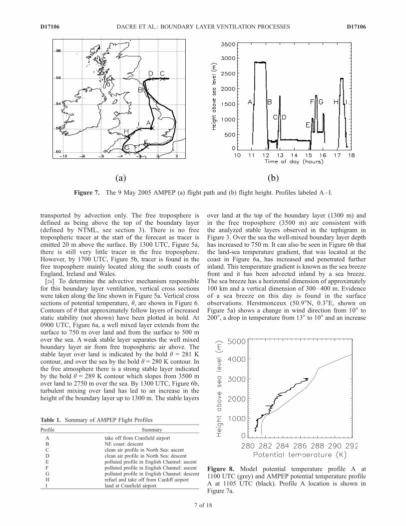
Figure 7. The 9 May 2005 AMPEP (a) flight path and (b) flight height. Profiles labeled A–I.

Table 1. Summary of AMPEP Flight Profiles

Profile Summary

A take off from Cranfield airportB NE coast: descentC clean air profile in North Sea: ascentD clean air profile in North Sea: descentE polluted profile in English Channel: ascentF polluted profile in English Channel: ascentG polluted profile in English Channel: descentH refuel and take off from Cardiff airportI land at Cranfield airport

Figure 8. Model potential temperature profile A at1100 UTC (grey) and AMPEP potential temperature profileA at 1105 UTC (black). Profile A location is shown inFigure 7a.


7 of 18

D17106

in humidity from 45% to 71% between 1200 UTC and1300 UTC (not shown). By 1700 UTC, Figure 6c, theboundary layer heights are similar to those at 1300 UTCwith the free atmospheric stable layer rising to 4000 m overland. The sea breeze front has retreated back toward thecoastline. In Figures 6a–6c the dotted line represents theNTML. The NTML approximately follows the height ofthe lowest stable layer. This leads to a sharp decrease inboundary layer height on crossing from land to sea in theafternoon. Polluted air may be transported into the freetroposphere here because of coastal outflow.[25] On 9 May 2005 AMPEP performed a flight clock-

wise around England (Figure 7a). During the flight verticalprofiles through the depth of the boundary layer were made.These profiles have been labeled A–I, Figure 7b, and aresummarized in Table 1. Figure 8 shows the model q profileat 1100 UTC and the AMPEP q vertical profile at 1105 UTCtaken in the middle of the UK (AMPEP profile A, locationshown in Figure 7a). The model vertical profile shows awell mixed boundary layer extending from the surface to1000 m. A stable layer at 1000 m separates the boundarylayer air from the free tropospheric air. There is also a freetropospheric stable layer at 3500 m. The AMPEP q verticalprofile also shows a well mixed boundary layer with a depthof 1000 m. The free tropospheric stable layer is not capturedas the profile only extends to 3000 m. Thus the model qprofile is consistent with the observations over land duringthe morning. Figure 9 shows the model q profile at1500 UTC and two AMPEP q vertical profiles at1506 UTC and 1524 UTC. These profiles are taken overthe English Channel (AMPEP profiles E and F, locationsshown in Figure 7a). The model profile shows two low-level stable layers, one at 300 m and another at 1000 m.There is also a free tropospheric stable layer at 3500 m. TheAMPEP q vertical profiles show stable layers at 300 m and1000 m which are consistent with the model profiles. Thuswe can conclude that the model representation of the stablelayers shown in Figure 6 are also realistic over the sea.

[26] Figure 10 shows vertical cross sections of tracerconcentration along the line shown in Figure 5a overplottedwith the bold potential contours from Figures 6a–6c. Traceris transported by advection only. Initially tracer remainsnear the surface in the lowest two model levels (Figure 10a).However at 1300 UTC, Figure 10b, tracer is advected up to1000 m in height just inland from the coast. By 1700 UTC,Figure 10c, this tracer has been advected above the unpol-luted marine boundary layer and mainly remains trappedbetween the two stable layers over the sea resulting in alayer of tracer above a layer with no tracer. The verticaltransport of tracer away from the surface to the top of theboundary layer is due to convergence between the seabreeze and the prevailing northerly wind. Figure 11 showsthe model vertical velocity at 1400 UTC, 500 m above thesurface. The convergence line lies along the south coasts ofEngland and Ireland. Tracer is advected vertically awayfrom the surface to the top of the boundary layer. The traceris then advected horizontally across the coast by theprevailing wind. Thus tracer is transported into the freetroposphere above the marine boundary layer by the coastaloutflow mechanism. Although there is a sea breeze acting inthis case, a sea breeze is not needed for coastal outflow tooccur. Turbulent mixing (seen in section 6.2) can alsotransport tracer up to the top of the boundary layer overland where it is then advected horizontally out of theboundary layer across the coast. A sea breeze can howeverincrease the amount of pollution ventilated by coastaloutflow. Advection across the coast could in part also bedue to the return flow of the sea breeze circulation. Strongeroffshore winds will lead to greater ventilation by coastaloutflow but will prevent the sea breeze from penetratingonshore. Weaker offshore winds will reduce ventilation bycoastal outflow but will allow the sea breeze to penetrateonshore resulting in greater ventilation by the sea breezecirculation.[27] The advective mechanisms responsible for ventilat-

ing the boundary layer in this nonfrontal case are verticaladvection, due to convergence between the sea breeze andthe prevailing wind, and coastal outflow. Mountain ventingand warm and cold conveyor belt advective transport arenot observed. The overall importance of the sea breezecirculation and coastal outflow in ventilating the boundarylayer is discussed in section 8.

6.2. Advection and Turbulent Mixing

[28] Figure 12 shows the tracer in the free troposphereintegrated over height for the tracer transported by advec-tion and boundary layer turbulent mixing. Turbulent mixingentrains tracer free air from above the boundary layerdiluting the concentration of the tracer in the boundarylayer. Thus the tracer concentrations are much reducedcompared to the tracer transported by advection only. At1300 UTC, Figure 12a, tracer has been transported out ofthe boundary layer along the south coasts of England,Ireland and Wales. Thus coastal outflow is observed earlierthan when tracer is transported by advection only. There isalso some free tropospheric tracer over land. By 1700 UTC,Figure 12b, tracer has been transported out of the boundarylayer over much of the UK and Ireland. Figure 13 showsvertical cross sections of tracer concentration for thetracer transported by advection and turbulent mixing. At

Figure 9. Model potential temperature profile E at 1500UTC(grey) and AMPEP potential temperature profile E at1506 UTC (black, 0–1000 m) and profile F at 1524 UTC(black, 600–1800 m). Profile E and F locations are shownin Figure 7a.


8 of 18

D17106

0900 UTC, Figure 13a, tracer has been mixed throughoutthe depth of the boundary layer over land. Tracer isadvected off the coast over the sea, remaining within themarine boundary layer as in the advection only case.[29] At 0900 UTC convergence over the sea allows a

build up of tracer, emitted over land, to form off the southcoast. By 1300 UTC, Figure 13b, the maximum in tracerconcentration is now inland as for the advection only tracer,Figure 10b. Vertical motion, due to convergence betweenthe sea breeze and the prevailing wind, transports sometracer out of the boundary layer at the coast. By 1700 UTC,Figure 13c, coastal outflow has advected high concentra-

Figure 10. Vertical cross sections of tracer concentration, contours every 200 � 10�7 kg/kg starting at10 � 10�7 kg/kg, overlaid with potential temperature contours from Figure 6, at (a) 0900 UTC,(b) 1300 UTC and (c) 1700 UTC. Tracer transported by advection only.

Figure 11. The 500 m vertical velocity at 1400 UTC,contours every 0.05 ms�1.


9 of 18

D17106

tions of tracer above the marine boundary layer. Weakvertical ascent over the whole of the UK between 500 mand 4 km (not shown) advects tracer that has been mixed byturbulence within the boundary layer out of the boundarylayer up to 2500 m. However, this tracer has not becomeseparated from the boundary layer tracer and is transportedat the same speed and in the same direction as the boundarylayer tracer. The ascent rates at the boundary layer top areconsistent with the distance traveled by the tracer. Thisimplies that other processes that could lead to this transport,such as mixing in the stable air and numerical diffusion, arenegligible.[30] In summary, turbulent mixing is responsible for

transporting tracer away from the surface and distributingit throughout the boundary layer. Turbulent mixing can alsotransport tracer to above the boundary layer top where it canthen be transported by the large-scale flow reaching heightsof 2500 m and some tracer is advected above the marineboundary layer by coastal outflow. The overall importanceof turbulent mixing and large-scale ascent in the ventilationof the boundary layer is discussed in section 8.

6.3. Advection, Turbulent Mixing, and Convection

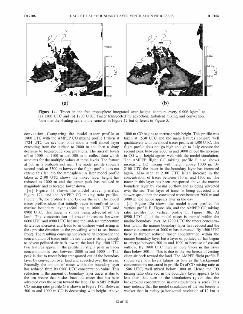
[31] Consider now the role of convection. Figure 14shows the tracer in the free troposphere integrated overheight for the case in which the tracer is transported byadvection, convection and turbulent mixing. These figuresare dramatically different from Figures 5 and 12 showingthat convection is an important process on this day. By1300 UTC, Figure 14a, there is tracer in the free troposphereover most of the land. By 1700 UTC, Figure 14b, theamount of tracer in the free troposphere has increasedas convection continues to transport tracer into the freetroposphere throughout the day. Tracer that has been trans-ported into the free troposphere is advected southeastwardover France while tracer that remains within the boundarylayer is advected southwestward into the north Atlantic (notshown).

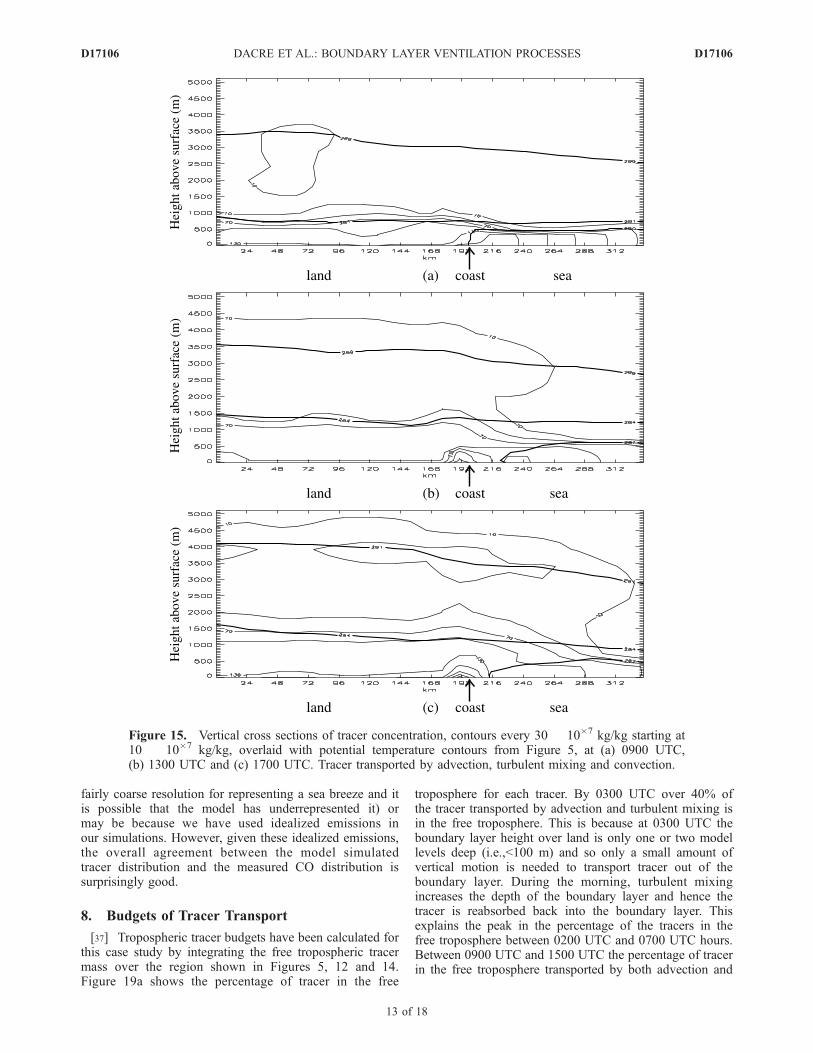
[32] Figure 15 shows vertical cross sections of tracerconcentration for the tracer transported by advection, mixingand convection. At 0900 UTC, Figure 15a, the tracerdistribution is very similar to Figure 13a when transportis by advection and turbulent mixing only. Tracer has beenmixed throughout the depth of the boundary layer overland and advection has transported tracer into the marineboundary layer over the sea. A small amount of tracer hasbeen transported up to the free tropospheric stable layer at3500 m. By 1300 UTC, Figure 15b, the amount of tracerthat has been transported up to 3500 m has increased asconvection continues to transport tracer vertically. Again,we can see a maximum in tracer concentration at the coast,but the concentration is lower than for the tracer transportedby advection and turbulent mixing as convection hasreduced the amount of tracer in the boundary layer. By1700 UTC, Figure 15c, the tracer transported to 3500 m hasformed a distinct layer. This separate layer is transportedfaster in the horizontal than the tracer that remains withinthe boundary layer. Thus including convection transportsmore tracer into the free troposphere, transports tracerhigher up in the atmosphere and reduces tracer in theboundary layer so less is available for transport by coastaloutflow and the sea breeze circulation. The overall impor-tance of this shallow convection in ventilating the boundarylayer is discussed in section 8.

7. Comparison With Observations

[33] In this section the results from the 3-D modelsimulation will be compared qualitatively to the CO meas-urements taken during the AMPEP campaign (http://badc.nerc.ac.uk/data/polluted-tropo/projects/ampep.html). COwas the chemical measured in AMPEP that is most similarto a passive tracer. It is emitted in urban areas and has alifetime of about 2 months. We do not expect quantitativeagreement between the tracer and measured CO because wehave used an idealized tracer distribution. Nevertheless it is

Figure 12. Tracer in the free troposphere integrated over height, contours every 0.006 kg/m2 at(a) 1300 UTC and (b) 1700 UTC. Tracer transported by advection and turbulent mixing. Note thedifferent shading scale to Figure 5.


10 of 18

D17106

interesting to make qualitative comparisons. Qualitativecomparisons between the model tracer that is transportedby advection, turbulent mixing and convection and theAMPEP CO measurements are made. Three profiles havebeen chosen for comparison. Profile I is over the land and itshows the depth of the boundary layer. Profile G is off thesouth coast of the UK and it shows high CO concentrationsabove the boundary layer, due to convection. Profile E isalso off the south coast of the UK and it shows low COconcentrations in the boundary layer, due to the sea breeze.[34] Figure 16 shows the model tracer profiles at different

times, Figure 16a, and the AMPEP CO mixing ratio profile,

Figure 16b, for vertical profile I in the middle of the UK. Asecond profile, profile D, has also been plotted. Profile Dwas taken out in the North Sea to provide a backgroundreference CO mixing ratio for this day as the air there isunpolluted. The model tracer profile at this location showsno tracer (and is not shown here). The model tracer profileat location I at 0600 UTC shows that the tracer is trappedwithin the lowest 650 m of the atmosphere. By 1200 UTCthe model tracer has been uniformly mixed up to 1200 m, itthen decreases sharply up to 1600 m. A second peak intracer concentration can be seen between 3000 m and4000 m. This is the tracer that has been transported by

Figure 13. Vertical cross sections of tracer concentration, contours every 30 � 10�7 kg/kg starting at10 � 10�7 kg/kg, overlaid with potential temperature contours from Figure 5, at (a) 0900 UTC,(b) 1300 UTC and (c) 1700 UTC. Tracer transported by advection and turbulent mixing.


11 of 18

D17106

convection. Comparing the model tracer profile at1800 UTC with the AMPEP CO mixing profile I taken at1724 UTC we see that both show a well mixed layerextending from the surface to 2000 m and then a sharpdecrease to background concentrations. The aircraft levelsoff at 1500 m, 1100 m and 500 m to collect data whichaccounts for the multiple values at these levels. The featureat 500 m is probably not real. The model profile shows asecond peak at 3300 m however the flight profile does notextend this far into the atmosphere. A later model profiletaken at 2100 UTC shows the mixed layer height hasreduced to 1000 m and the upper peak has reduced inmagnitude and is located lower down.[35] Figure 17 shows the model tracer profiles,

Figure 17a, and the AMPEP CO mixing ratio profiles,Figure 17b, for profiles F and G over the sea. The modeltracer profiles show that initially tracer is confined to themarine boundary layer (<500 m) at 0600 UTC and0900 UTC. This tracer is simply being advected off theland. The concentration of tracer increases between0600 UTC and 0900 UTC because the land-sea temperaturedifference increases and leads to an onshore wind acting inthe opposite direction to the prevailing wind (a sea breezefront). The resulting convergence leads to an increase in theconcentration of tracer until the sea breeze is strong enoughto advect polluted air back toward the land. By 1500 UTCtwo features appear in the profile. Firstly, a peak in tracerconcentration is seen between 2000 m and 3000 m. Thispeak is due to tracer being transported out of the boundarylayer by convection over land and advected over the ocean.Secondly, the amount of tracer within the boundary layerhas reduced from its 0900 UTC concentration value. Thisreduction in the amount of boundary layer tracer is due tothe sea breeze that pushes back the tracer that has beenadvected over the ocean toward the land. The AMPEP flightCO mixing ratio profile G is shown in Figure 17b. Between500 m and 1000 m CO is decreasing with height. Above

1000 m CO begins to increase with height. This profile wastaken at 1530 UTC and the main features compare wellqualitatively with the model tracer profile at 1500 UTC. Theflight profile does not go high enough to fully capture thesecond peak between 2000 m and 3000 m but the increasein CO with height agrees well with the model simulation.The AMPEP flight CO mixing profile F also showsincreasing CO mixing with height above 1000 m. By2100 UTC the tracer in the boundary layer has increasedagain. Also seen at 2100 UTC is an increase in theconcentration of tracer between 750 m and 1500 m. Thetracer in this layer has been transported above the marineboundary layer by coastal outflow and is being advectedover the sea. This layer of tracer is being advected at aslower speed than the convected tracer between 2000 m and3000 m and hence appears later in the day.[36] Figure 18a shows the model tracer profiles for

vertical profile E, Figure 18a, and the AMPEP CO mixingratio profiles for vertical profile E, Figure 18b. At0900 UTC all of the model tracer is trapped within themarine boundary layer. At 1200 UTC the tracer concentra-tion within the marine boundary layer has reduced and thetracer concentration at 3000 m has increased. By 1500 UTCthere is further reduced tracer concentration within themarine boundary layer but a layer of polluted air has begunto emerge between 500 m and 1000 m because of coastaloutflow. By 1800 UTC there is more tracer in this layerthan below 500 m. This is due to the sea breeze advectingclean air back toward the land. The AMPEP flight profile Eshows very low levels (almost as low as the backgroundconcentrations measured in profile D) of CO mixing ratio at1506 UTC, well mixed below 1000 m. Hence the COmixing ratio observed in the boundary layer appears to beless than that seen in the simulations (given that thebackground concentration in our simulations is zero). Thismay indicate that the model simulation of the sea breeze isweaker than in reality (a horizontal resolution of 12 km is

Figure 14. Tracer in the free troposphere integrated over height, contours every 0.006 kg/m2 at(a) 1300 UTC and (b) 1700 UTC. Tracer transported by advection, turbulent mixing and convection.Note that the shading scale is the same as in Figure 12 but different to Figure 5.


12 of 18

D17106

fairly coarse resolution for representing a sea breeze and itis possible that the model has underrepresented it) ormay be because we have used idealized emissions inour simulations. However, given these idealized emissions,the overall agreement between the model simulatedtracer distribution and the measured CO distribution issurprisingly good.

8. Budgets of Tracer Transport

[37] Tropospheric tracer budgets have been calculated forthis case study by integrating the free tropospheric tracermass over the region shown in Figures 5, 12 and 14.Figure 19a shows the percentage of tracer in the free

troposphere for each tracer. By 0300 UTC over 40% ofthe tracer transported by advection and turbulent mixing isin the free troposphere. This is because at 0300 UTC theboundary layer height over land is only one or two modellevels deep (i.e.,<100 m) and so only a small amount ofvertical motion is needed to transport tracer out of theboundary layer. During the morning, turbulent mixingincreases the depth of the boundary layer and hence thetracer is reabsorbed back into the boundary layer. Thisexplains the peak in the percentage of the tracers in thefree troposphere between 0200 UTC and 0700 UTC hours.Between 0900 UTC and 1500 UTC the percentage of tracerin the free troposphere transported by both advection and

Figure 15. Vertical cross sections of tracer concentration, contours every 30 � 10�7 kg/kg starting at10 � 10�7 kg/kg, overlaid with potential temperature contours from Figure 5, at (a) 0900 UTC,(b) 1300 UTC and (c) 1700 UTC. Tracer transported by advection, turbulent mixing and convection.


13 of 18

D17106

turbulent mixing and by advection, turbulent mixing andconvection increases. However the difference between thesetwo curves gradually increases. This is because convectionis continually transporting extra tracer into the free tropo-sphere. By 1800 UTC, when the boundary layer heightcollapses, 52% of the tracer transported by advection,turbulent mixing and convection and 46% of the tracertransported by advection and turbulent mixing is in the freetroposphere. At 1200 UTC, when the sea breeze starts, thepercentage of tracer transported by advection begins toincrease from 0% to 26% by 1800 UTC. At 1800 UTCthe height of the boundary layer collapses. This leads to a

sharp increase in the percentage of free tropospheric traceras tracer that was within the boundary layer now finds itselfabove the boundary layer top. Even during a nonfrontal dayover half of the tracer emitted in the boundary layer istransported to the free troposphere. Turbulent mixing andconvective processes doubled the amount of ventilation andhence need to be represented in chemical transport models.[38] The further tracer is removed vertically from the

boundary layer the further it is likely to be horizontallytransported. Figure 19b shows the percentage of tracerabove 2000 m for each tracer. At the beginning of the dayall of the tracers remain below 2000 m. After 0900 UTC

Figure 16. (a) Model tracer profile I at selected times and (b) AMPEP CO mixing profile D (left curve)at 1300 UTC and AMPEP CO mixing profile I (right curve) at 1724 UTC.

Figure 17. (a) Model tracer profile G at selected times and (b) AMPEP CO mixing and profile F at1524 UTC (right curve) and profile G at 1534 UTC (left curve).


14 of 18

D17106

there is an increase in the percentage of tracer above 2000 mfor the tracer that is transported by advection, turbulentmixing and convection. This is due to tracer being trans-ported out of the boundary layer in the convectiveupdraughts. It reaches a peak of 26% at 1700 UTC whenconvection dies down and then begins to decrease becausetracer is being advected out of the domain. Advection andturbulent mixing transports a maximum of 10% of the tracerabove 2000 m, while only 2% of the tracer transportedby advection only is transported above 2000 m. Thusconvection is essential to transport tracer high in theatmosphere where it is likely to become sheared from thelow-level tracer.

[39] We have seen from the vertical cross sections inFigures 13 and 15 that some tracer remains just above theboundary layer top staying connected to the boundary layertracer. This tracer has been transported above the boundarylayer top by turbulent mixing followed by large-scaleascent. The amount of tracer transported will thus besensitive to the definition of the boundary layer height.By contrast, tracer transported out of the boundary layer byconvection reaches 3.5 km and so is not sensitive to thedefinition of the boundary layer. While the precise percen-tages of transport by each process will change if a slightlyhigher or lower boundary layer top definition is used themain conclusion, that the processes identified can all lead

Figure 18. (a) Model tracer profile E at selected times and (b) AMPEP COmixing profile E at 1506 UTC.

Figure 19. Time series of tracer integrated over the domain shown in Figure 7a. Percentage of tracerabove (a) the boundary layer and (b) 2000 m. Tracer transported by advection (dashed); advection andturbulent mixing (dotted); and advection, turbulent mixing and convection (solid).


15 of 18

D17106

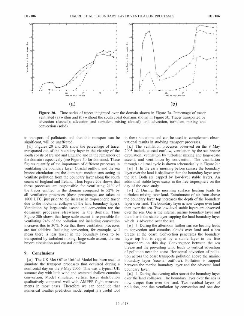
to transport of pollutants and that this transport can besignificant, will be unaffected.[40] Figures 20 and 20b show the percentage of tracer

transported out of the boundary layer in the vicinity of thesouth coasts of Ireland and England and in the remainder ofthe domain respectively (see Figure 5b for domains). Thesefigures quantify of the importance of different processes inventilating the boundary layer. Coastal outflow and the seabreeze circulation are the dominant mechanisms acting toventilate pollution from the boundary layer along the southcoasts of England and Ireland. Thus Figure 20a shows thatthese processes are responsible for ventilating 21% ofthe tracer emitted in the domain compared to 52% byall ventilation processes (these percentages are taken at1800 UTC, just prior to the increase in tropospheric tracerdue to the nocturnal collapse of the land boundary layer).Ventilation by large-scale ascent and convection are thedominant processes elsewhere in the domain. ThusFigure 20b shows that large-scale ascent is responsible forventilating 24% of the pollution and including convectionincreases this to 30%. Note that these ventilation processesare not additive. Including convection, for example, willmean there is less tracer in the boundary layer to betransported by turbulent mixing, large-scale ascent, the seabreeze circulation and coastal outflow.

9. Conclusions

[41] The UK Met Office Unified Model has been used tosimulate the transport processes that occurred during anonfrontal day on the 9 May 2005. This was a typical UKsummer day with little wind and scattered shallow cumulusconvection. Model simulated vertical tracer distributionqualitatively compared well with AMPEP flight measure-ments in most cases. Therefore we can conclude thatnumerical weather prediction model output is a useful tool

in these situations and can be used to complement obser-vational results in studying transport processes.[42] The ventilation processes observed on the 9 May

2005 include coastal outflow, ventilation by the sea breezecirculation, ventilation by turbulent mixing and large-scaleascent, and ventilation by convection. The ventilationthrough a diurnal cycle is shown schematically in Figure 21:[43] 1. In the early morning before sunrise the boundary

layer over the land is shallower than the boundary layer overthe sea. Both are capped by low-level stable layers. Anadditional stable layer exists in the free troposphere on theday of the case study.[44] 2. During the morning surface heating leads to

turbulent mixing over land. Entrainment of air from abovethe boundary layer top increases the depth of the boundarylayer over land. The boundary layer is now deeper over landthan over the sea. Two low-level stable layers are observedover the sea. One is the internal marine boundary layer andthe other is the stable layer capping the land boundary layerwhich is advected over the sea.[45] 3. During the afternoon further surface heating leads

to convection and cumulus clouds over land and a seabreeze at the coast. Convection penetrates the boundarylayer top but is capped by a stable layer in the freetroposphere on this day. Convergence between the seabreeze and the prevailing wind leads to vertical advectionof pollution near the coast. Horizontal advection of pollu-tion across the coast transports pollution above the marineboundary layer (coastal outflow). Pollution is trappedbetween the marine boundary layer and the advected landboundary layer.[46] 4. During the evening after sunset the boundary layer

over the land collapses. The boundary layer over the sea isnow deeper than over the land. Two residual layers ofpollution, one due ventilation by convection and one due

Figure 20. Time series of tracer integrated over the domain shown in Figure 7a. Percentage of tracerventilated (a) within and (b) without the south coast domains shown in Figure 5b. Tracer transported byadvection (dashed); advection and turbulent mixing (dotted); and advection, turbulent mixing andconvection (solid).


16 of 18

D17106

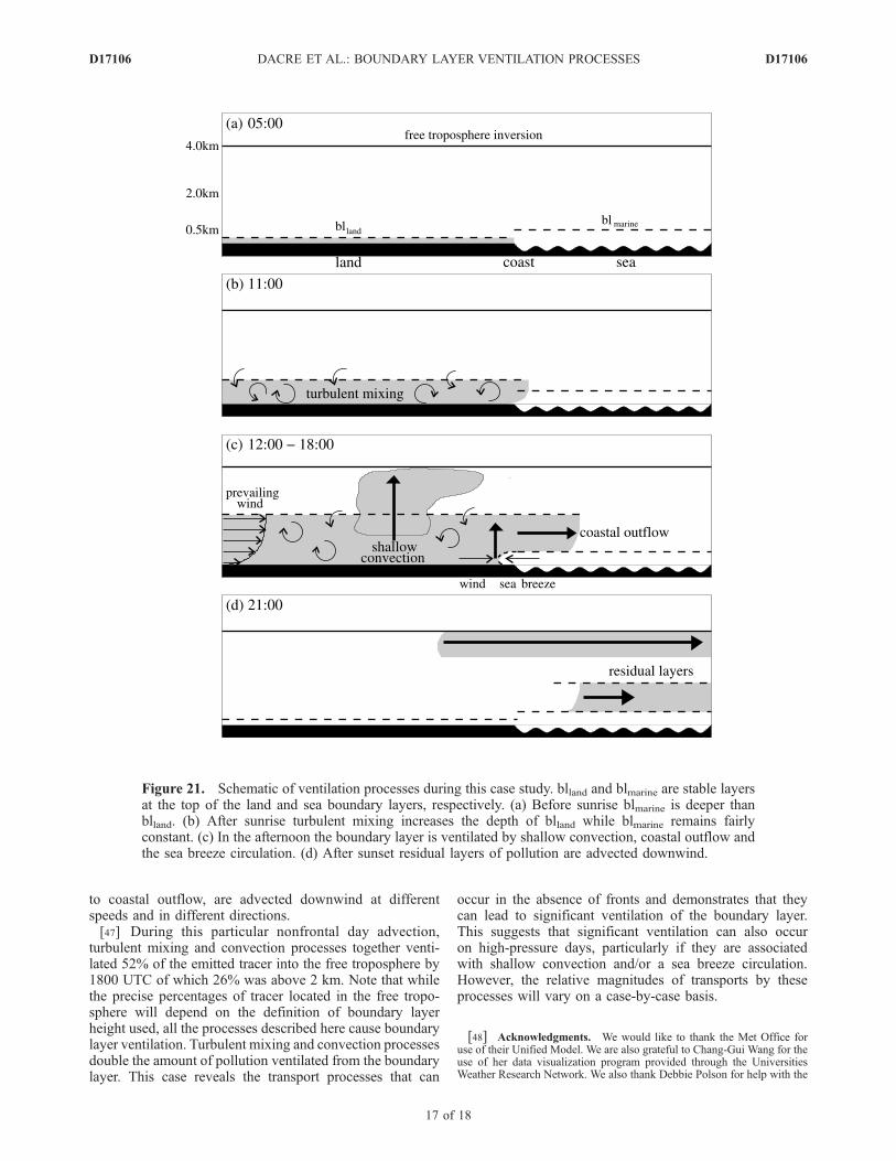
to coastal outflow, are advected downwind at differentspeeds and in different directions.[47] During this particular nonfrontal day advection,

turbulent mixing and convection processes together venti-lated 52% of the emitted tracer into the free troposphere by1800 UTC of which 26% was above 2 km. Note that whilethe precise percentages of tracer located in the free tropo-sphere will depend on the definition of boundary layerheight used, all the processes described here cause boundarylayer ventilation. Turbulent mixing and convection processesdouble the amount of pollution ventilated from the boundarylayer. This case reveals the transport processes that can

occur in the absence of fronts and demonstrates that theycan lead to significant ventilation of the boundary layer.This suggests that significant ventilation can also occuron high-pressure days, particularly if they are associatedwith shallow convection and/or a sea breeze circulation.However, the relative magnitudes of transports by theseprocesses will vary on a case-by-case basis.

[48] Acknowledgments. We would like to thank the Met Office foruse of their Unified Model. We are also grateful to Chang-Gui Wang for theuse of her data visualization program provided through the UniversitiesWeather Research Network. We also thank Debbie Polson for help with the

Figure 21. Schematic of ventilation processes during this case study. blland and blmarine are stable layersat the top of the land and sea boundary layers, respectively. (a) Before sunrise blmarine is deeper thanblland. (b) After sunrise turbulent mixing increases the depth of blland while blmarine remains fairlyconstant. (c) In the afternoon the boundary layer is ventilated by shallow convection, coastal outflow andthe sea breeze circulation. (d) After sunset residual layers of pollution are advected downwind.


17 of 18

D17106

AMPEP data and all of the AMPEP team for taking the aircraft measure-ments. Helen Dacre was supported by a NERC grant.

ReferencesAgustı-Panareda, A., S. L. Gray, and J. Methven (2005), Numerical mod-eling study of boundary-layer ventilation by a cold front over Europe,J. Geophys. Res., 110, D18304, doi:10.1029/2004JD005555.

Angevine, W. M., M. Tjernstrom, and M. Zagar (2006), Modeling of thecoastal boundary layer and pollutant transport in New England, J. Appl.Meteorol. Climatol., 138(45), 137–154.

Baltensperger, U., H. W. Gaggeler, D. T. Jost, M. Lugauer, M. Schwikowski,E. Weingartner, and P. Seibert (1997), Aerosol climatology at the high-alpine site Jungfraujoch, Switzerland, J. Geophys. Res., 102, 19,707–19,715.

Chatfield, R. B., and P. J. Crutzen (1984), Sulfur dioxide in remote oceanicair: Cloud transport of reactive precursors, J. Geophys. Res., 89, 7111–7132.

Cullen, M. (1993), The unified forecast/climate model, Meteorol. Mag.,122, 81–94.

Dickerson, R. R., et al. (1987), Thunderstorms: An important mechanism inthe tranport of air pollutants, Science, 235, 460–465.

Donnell, E. A., D. J. Fish, and E. M. Dicks (2001), Mechanisms for pollu-tant transport between the boundary layer and the free troposphere,J. Geophys. Res., 106(D8), 7847–7856.

Edy, J., S. Cautenet, and P. Bremaud (1996), Modeling ozone and carbonmonoxide redistribution by shallow convection over the Amazonian rainforest, J. Geophys. Res., 101(D22), 28,671–28,681.

Esler, J. G., P. H. Haynes, K. S. Law, H. Barjat, K. Dewey, J. Kent, andS. Schmitgen (2003), Transport and mixing between airmasses in coldfrontal regions during Dynamics and Chemistry of Frontal Zones(DCFZ), J. Geophys. Res., 108(D4), 4142, doi:10.1029/2001JD001494.

Flatøy, F., and Ø. Hov (1995), Three-dimensional model studies ofexchange processes of ozone in the troposphere over Europe, J. Geophys.Res., 100(D6), 11,465–11,481.

Gimson, N. R. (1997), Pollution transport by convective clouds in amesoscale model, Q. J. R. Meteorol. Soc., 123, 1805–1828.

Gray, S. L. (2003), A case study of stratosphere to troposphere transport:The role of convective transport and the sensitivity to model resolution,J. Geophys. Res., 108(D18), 4590, doi:10.1029/2002JD003317.

Gregory, D., and P. R. Rowntree (1990), A mass flux convection schemewith representation of cloud ensemble characteristics and stability depen-dent closure, Mon. Weather Rev., 118, 1483–1506.

Hauf, T., P. Schulte, R. Alheit, and H. Schlager (1995), Rapid vertical tracergas transport by an isolated midlatitude thunderstorm, J. Geophys. Res.,100(D11), 22,957–22,970.

Hobbs, P. V. (2000), Introduction to Atmospheric Chemistry, CambridgeUniv. Press, Cambridge, U. K.

Kossmann, M., U. Corsmeier, S. De Wekker, F. Fiedler, R. Vogtlin,N. Kalthoff, H. Gustin, and B. Neininger (1999), Observations of hand-over processes between the atmospheric boundary layer and the freetroposphere overm ountainous terrain, Contrib. Atmos. Phys., 72, 329–350.

Kowol-Santen, J., M. Beekman, S. Schmitgen, and K. Dewey (2001),Tracer analysis of transport from the boundary layer to the free tropo-sphere, Geophys. Res. Let., 28, 2907–2910.

Leon, J.-F., et al. (2001), Large-scale advection of continental aerosolsduring INDOEX, J. Geophys. Res., 106(D22), 28,427–28,439.

Lock, A. P., A. R. Brown, M. R. Bush, G. M. Martin, and R. N. B. Smith(2000), A new boundary layer mixing scheme. Part 1. Scheme descrip-tion and single-column model tests, Mon. Weather Rev., 128, 187–199.

Lu, R., and R. Turco (1994), Air pollutant transport in a coastal environ-ment. Part I: Two-dimensional simulations of sea-breeze and mountaineffects, J. Atmos. Sci., 51, 2285–2308.

Lu, R., C. Lin, R. Turco, and A. Arakawa (2000), Cumulus transport ofchemical tracers: 1. Cloud-resolving model simulations, J. Geophys. Res.,105(D8), 10,001–10,021.

Schultz, P., and T. T. Warner (1982), Characteristics of summertime circula-tions and pollutant ventilation in the Los Angeles basin, J. Appl. Meteorol.,21, 672–682.

Seibert, P., H. Kromp-Kolb, A. Kasper, M. Kalina, H. Puxbaum, D. T. Jost,M. Schwikowski, and U. Baltensperger (1998), Transport of pollutedboundary layer air from the PoValley to high-alpine sites,Atmos. Environ.,32, 3953–3965.

Smith, F. B. (1975), Airborne transport of sulphur dioxide from the UnitedKingdom, Atmos. Environ., 9, 643–659.

Thompson, A. M., K. E. Pickering, R. R. Dickerson, W. G. Ellis Jr., D. J.Jacob, J. R. Scala, W.-K. Tao, D. P. McNamara, and J. Simpson (1994),Convective transport over the central United States and its rode in regionalCO and ozone budgets, J. Geophys. Res., 99(D9), 18,703–18,711.

Verma, S., O. Boucher, C. Vendataraman,M. S. Reddy, D. Muller, P. Chazette,and B. Crouzille (2006), Aerosol lofting from sea breeze during the IndianOcean experiment, J. Geophys. Res., 111, D07208, doi:10.1029/2005JD005953.

Wakimoto, R. M., and J. L. McElroy (1986), Lidar observation of elevatedpollution layers over Los Angeles, J. Clim. Appl. Meteorol., 25, 1583–1599.

Wang, C., and R. G. Prinn (2000), On the roles of deep convective clouds intropospheric chemistry, J. Geophys. Res., 105(D17), 22,269–22,287.

Wilson, D. R., and S. P. Ballard (1999), A microphysically based precipita-tion scheme for the UK Meteorological Office unified model, Q. J. R.Meteorol. Soc., 125, 1607–1636.

��S. E. Belcher, H. F. Dacre, and S. L. Gray, Department of Meteorology,

University of Reading, Earley Gate, PO Box 243, Reading RG6 6BB, UK.([email protected])


18 of 18

D17106

A case study of boundary layer ventilation by convection...

Documents

Transcript of A case study of boundary layer ventilation by convection...