A Case Control Study of Speed and Crash Risk

Technical Report 2

Bayesian Reconstruction of Traffic Accidents and the Causal Effect of

Speed in Intersection and Pedestrian Accidents

Final Report

Prepared by: Gary A. Davis

Department of Civil Engineering

University of Minnesota

CTS 06-01B

HUMAN CENTERED TECHNOLOGY TO ENHANCE SAFETY AND TECHNOLOGY

Technical Report Documentation Page 1. Report No. 2. 3. Recipients Accession No.

CTS 06-01B 4. Title and Subtitle 5. Report Date

April 2006 6.

A Case Control Study of Speed and Crash Risk Technical Report 2 Bayesian Reconstruction of Traffic Accidents and the Casual Effect of Speed in Intersection and Pedestrian Accidents

7. Author(s) 8. Performing Organization Report No.

Gary A. Davis 9. Performing Organization Name and Address 10. Project/Task/Work Unit No.

CTS Project Number 2001032 11. Contract (C) or Grant (G) No.

Department of Civil Engineering University of Minnesota 500 Pillsbury Dr SE Minneapolis, MN 55455

12. Sponsoring Organization Name and Address 13. Type of Report and Period Covered

Final Report December 2000-February 2002 14. Sponsoring Agency Code

Intelligent Transportation Systems Institute Center for Transportation Studies University of Minnesota 511 Washington Avenue SE, Suite 200 Minneapolis, MN 55455

15. Supplementary Notes

http://www.cts.umn.edu/pdf/CTS-06-01B.pdf 16. Abstract (Limit: 200 words)

Traffic accident reconstruction has been defined as the effort to determine, from whatever evidence is available, how an accident happened. Traffic accident reconstruction can be treated as a problem in uncertain reasoning about a particular event, and developments in modeling uncertain reasoning for artificial intelligence can be applied to this problem. Physical principles can usually be used to develop a structural model of the accident and this model, together with an expert assessment of prior uncertainty regarding the accident’s initial conditions, can be represented as a Bayesian network. Posterior probabilities for the accident’s initial conditions, given evidence collected at the accident scene, can then be computed by updating the Bayesian network. Using a possible worlds semantics, truth conditions for counterfactual claims about the accident can be defined and used to rigorously implement a “but for” test of whether or not a speed limit violation could be considered a cause of an accident. The logic of this approach is illustrated for a simplified version of a vehicle/pedestrian accident, and then the approach is applied to determine the causal effect of speeding in 10 actual accidents.

17. Document Analysis/Descriptors 18.Availability Statement

Bayes’ theorem, accident reconstruction, accident causes, speed limits, traffic accidents

No restrictions. Document available from: National Technical Information Services, Springfield, Virginia 22161

19. Security Class (this report) 20. Security Class (this page) 21. No. of Pages 22. Price

Classified Classified 43

A Case Control Study of Speed and Crash Risk Technical Report 2

Bayesian Reconstruction of Traffic Accidents and the Causal Effect of Speed in Intersection and

Pedestrian Accidents

Final Report

Prepared by: Gary A. Davis

Department of Civil Engineering

University of Minnesota

April 2006

Intelligent Transportation Systems Institute Center for Transportation Studies

University of Minnesota

CTS 06-01B

This report represents the results of research conducted by the authors and does not necessarily reflect the official views or policy of the Center for Transportation Studies or the University of Minnesota.

Acknowledgements

The author wishes to acknowledge those who made this research possible.

Funding for the study was provided by the Intelligent Transportation Systems (ITS)

Institute at the University of Minnesota’s Center for Transportation Studies (CTS). The

ITS Institute is a program funded by the United States Department of Transportation

(USDOT) and administered by the USDOT's Research and Innovative Technologies

Administration (RITA).

A Case Control Study of Speed and Crash Risk

Technical Report 2

Bayesian Reconstruction of Traffic Accidents and the Causal Effect of Speed in Intersection

and Pedestrian Accidents

Gary A. Davis

University of Minnesota

In Technical Report 1 for this project we argued that traffic accidents should be treated as resulting

from the workings of partially understood, deterministic processes, and that the causal effect of some

variable could, at least in principle, be determined "bottom up," by considering that variable's effect on each

of a set of individual accidents. Since this requires that we reason in a logical manner about the uncertainty

attached to particular events, we are faced with a problem more like determining an individual's cause of

death, or identifying the perpetrator of a crime, than like estimating a summary measure for some population

of entities. At the First International Conference on Forensic Statistics Lindley (1991) argued that the

probability calculus should be applied not only to statistical problems, but to forensic inference more

generally. Lindley focused on a class of problems for which the hypotheses of interest were the guilt or

innocence of a defendant, and the task was to weigh the plausibility of these alternatives in the light of

evidence. His proposed solution was Bayesian, where one first determines a prior assignment of probability

to the alternative hypotheses, along with the probability of the evidence given each alternative, and then uses

Bayes theorem to compute posterior probabilities for the hypotheses. This approach has since been applied

to increasingly more complicated problems in forensic identification (e.g. Balding 2000; Dawid and

Mortera 1998), in part due to an intense interest in interpreting DNA evidence.

Forensic Inference and Traffic Accidents

Lindley also referred briefly to a different class of problems, exemplified by "the case of a motorist

charged with dangerous drivingYHere the possible criminal is known; what is in doubt is whether there was

a crime" (1991, p. 86). Such problems are most prominent when a traffic accident has resulted in death or

serious injury, and it must be determined if a driver should be subjected to criminal or civil penalties. The

specific conditions which define this liability vary somewhat across jurisdictions, but it is generally possible

to identify two basic issues, pertaining to the quality of driving, and to the causal relation between the driving

and the accident's outcome. For example, in Great Britain "causing death by dangerous driving" occurs

when "a person causes the death of another person by driving a mechanically propelled vehicle

dangerously" while "dangerous driving" is in turn defined as driving that "falls far below what would be

expected of a competent and careful driver" (Road Traffic Act 1991). In the United States, the Uniform

Vehicle Code states that "homicide by vehicle" occurs when a driver "is engaged in the violation of any state

law or municipal ordinance applying to the operation or use of a vehicle" and when "such violation is the

proximate cause of said death" (NCUTLO 1992). (Italics have been added for emphasis.)

For some accidents, eyewitness testimony may be reliable enough, and the driving egregious

enough, that questions concerning the quality of driving and its relation to the accident are readily resolved.

In other cases however the evidence can be entirely circumstantial, collected by accident investigators after

the event. The connections between the evidence and the basic legal issues can then be less clear, and over

the past 70 years the practice of accident investigation and reconstruction has developed primarily to assist

the legal system in resolving such questions (Traffic Institute 1946; Rudram and Lambourn 1981). Baker

and Fricke define accident reconstruction as "the effort to determine, from whatever information is available,

how the accident occurred" (1990, p. 50-3). Typical questions which a reconstructionist can be called on

to address include ascertaining the initial speeds and locations of the involved parties, identifying the actions

taken by these parties, and determining the degree to which avoidance actions might have been effective.

Rarely however will direct observations alone be sufficient to answer these questions, and the

reconstructionist may need to supplement the information collected at the accident's scene.

These issues can be illustrated by considering an instructional example used by Greatrix (2002). On

a summer afternoon in Carlisle, England, a seven year-old boy attempted to cross a road ahead of an

oncoming vehicle, and although the driver braked to a stop, the child was struck. Measurements made at

the scene yielded a skidmark 22 meters long, with the point of collision being 12 meters from the start of

the skid. It was also noted that the speed limit on the road was 30 mph (13.4 meters/sec). A standard

practice in accident reconstruction is to use, as additional premises, variants of the kinematic formula

s=vt+(at2)/2 (1)

which gives the distance s traveled during time interval t by an object with initial velocity v while undergoing

a constant acceleration of a. In this case, test skids conducted after the accident suggested that a braking

deceleration a=-7.24 meters/sec2 was plausible, and this value together with the measured skidmark of 22

meters gives the speed of the vehicle at the start of the skid as 17.8 meters/sec. Citing statistical evidence

on the distribution of driver reaction times (denoted here by tp), Greatrix used a representative value of 1.33

seconds to deduce that the vehicle was 35.7 meters from the collision point when the driver noticed the

pedestrian. If the vehicle has been traveling instead at the posted speed of 30 mph (13.4 meters/sec), the

driver would have needed only 30.2 meters to stop and so, other things equal, would not have hit the child.

Thus the evidence could be taken as supporting claims that the driver was speeding, and that had the driver

not been speeding, the accident would not have happened. At this point though a different expert could

argue that no one knows for certain either the actual braking deceleration or the driver's actual reaction time.

The alternative values of a=-5.5 meters/sec2 and tp=1.0 seconds imply that the magnitude of the speed limit

violation was only about 5 mph, and that the vehicle would not have stopped before reaching to collision

point, even if the initial speed had been 30 mph. It could then be claimed that both the degree to which the

driver's speed violated the speed limit, and the causal connection between that violation and the result, are

open to doubt.

One way to view this example is as an attempt to answer three types of questions. The first type,

which can be called factual questions, concerns the actual conditions associated with this particular accident.

These include the paths of the pedestrian and vehicle, the initial speed of the vehicle, and the relation

between this speed and the posted speed limit. Answering this type of question is what Baker and Fricke

consider the role of accident reconstruction proper. The second type, which can be called counterfactual

questions, starts with a stipulation of the facts, but then goes beyond these and attempts to determine what

would have happened had certain specific conditions been different. In the example, determining whether

or not the vehicle would have stopped before reaching the pedestrian, had the initial speed been equal to

the posted limit, is a question of this type. Counterfactual questions usually arise in accident reconstruction

when attempting to identify what Baker called "causal factors," which are circumstances "contributing to

a result without which the result could not have occurred" (Baker 1975, p.274). Posing and answering

counterfactual questions has been referred to as "avoidance analysis" (Limpert 1989), or "sequence of

events analysis" (Hicks 1989) in the accident reconstruction literature. Finally, the third type of question

arises because of uncertainty regarding the conditions of the accident, which leads to uncertainty concerning

the answers to the first two types of question.

How best to account for uncertainty in an accident reconstruction is currently an unresolved issue.

A common recommendation has been to perform sensitivity analyses, in which the values of selected input

variables are changed and estimates recomputed (Schochenhoff et al. 1985; Hicks 1989; Niederer 1991).

When the conclusions of the reconstruction (e.g. that the driver was speeding) are insensitive to this variation

they can be regarded as well-supported, but if different yet plausible combinations of input values produce

differing results, this approach is inconclusive. This limitation has been recognized, and has motivated several

authors to apply probabilistic methods. Brach (1994) has illustrated how the method of statistical

differentials can be used to compute the variance of an estimate, given a differentiable expression for the

desired estimate and a specification of the means and variances of distributions characterizing the uncertainty

in the expression's arguments. Kost and Werner (1994) and Wood and O’Riordain (1994) have suggested

that Monte Carlo simulation can be used for more complicated models where tractable solutions are not

at hand. The Monte Carlo methods also produce approximate probability distributions characterizing the

uncertainty of estimates, rather than just means and variances. Particularly interesting are the examples used

by Wood and O’Riordain, where simulated outcomes inconsistent with measurements were rejected, in

effect producing posterior conditional distributions for the quantities of interest. These posterior distributions

were then used to compute the probability of a counterfactual claim, that the accident would not have

occurred had a vehicle's initial speed been different. More recently, Rose et al. (2001) have employed a

Monte Carlo approach similar to that of Wood and O=Riordain. A weakness of this approach, rooted in

the appearance of the Borel paradox when making inferences using deterministic simulation models, has

been identified by Hoogstrate and Spek (2002), who used Bayesian melding (Poole and Raftery 2000) to

get around this problem. Roughly concomitant with the developing interest in probabilistic accident

reconstruction has been an interest in using Bayesian networks to support more traditional forensic inference

(Edwards 1991; Aitken et al. 1996; Dawid and Evett 1997; Curran et al., 1998). Bayesian networks can

be used to represent an expert's knowledge concerning some class of systems, together with his or her

uncertainty concerning the state of a particular system in that class. The system's state is characterized by

the values taken on by a set of variables, and the dependencies among the system variables are described

by specifying a set of deterministic and/or stochastic relationships (Jensen 1996). Davis (1999, 2001) has

illustrated how Bayesian network methods and Markov Chain Monte Carlo (MCMC) computational

techniques can be combined to accomplish a Bayesian reconstruction of vehicle/pedestrian accidents.

Despite this growing interest in using probabilistic reasoning in accident reconstruction, there

appears to be some confusion about the relation between these applications and traditional statistical

reasoning. Brach faulted sensitivity analyses because "the statistical nature of the variations is not explicitly

taken into account," (1994, p. 148), while Wood and O’Riordain referred to an expression giving the

coefficient of variation for an individual speed estimate as "..a statistical approach," (1994, p. 130). Rose

et al. recommended Monte Carlo simulation because it produces "statistically relevant conclusions regarding

the probable ∆V experienced by a vehicle" (2001, p. 2). These quotations suggest a tendency to view

probabilistic accident reconstruction as an exercise in statistical inference. Lindley (1991), and more recently

Schum (2000) have argued though that statistical inference problems are only a subset of the forensic

problems to which probabilistic methods can be applied. Although reasonable people can disagree on how

to define the discipline of statistics, statistical problems typically involve making inferences about how some

characteristic is distributed over a population of entities, using measurements made on a sample from that

population. Probabilities are used to express uncertainty about parameters characterizing the population

distribution, and this uncertainty can in principle be reduced by increasing the sample's size. In contrast, the

usual objective of an accident reconstruction is to make inferences about an individual event, and

probabilities are assigned to statements about that event. When an individual accident can be regarded as

exchangeable with the members of a reference population, pre-established characteristics of that population

could be used to make these probability assignments, but once the characteristics of the reference

distribution are known, information about additional accidents in the reference population reveals nothing

more about the accident at hand.

The confusion concerning the appropriate role of probability in accident reconstruction can at least

in part be attributed to two fundamentally different meanings attached to probability statements, on the one

hand referring to expected relative frequencies in repeated trials of "chance setups," (Hacking 1965) and

on the other referring to a degree of credibility assigned to propositions. This duality was apparently present

in the initial development of probability theory in the 17th century (Hacking 1975), recurs in philosophical

treatments of probability (e.g. Carnap 1945; Lewis 1980), and has reappeared in the study of logics for

artificial reasoning (Halpern 1990). The view we shall adopt here is that an accident reconstruction

produces expert opinion about a particular, past event. To quote Baker and Fricke: "Opinions or

conclusions are the products of accident reconstruction. To the extent that reports of direct observations

are available and can be depended on as facts, reconstruction is unnecessary." (1990, p. 50-4) Statements

of opinion can be more or less certain however, depending on the certainty attached to their premises. If

this uncertainty is graded using probabilities, then the probability calculus can be used as a logic to derive

the uncertainty attached to conclusions. This approach is what Howson (1993) calls "personalistic

Bayesianism" but before continuing it should be noted that it is by no means the only alternative available.

Debate continues as to when or even if the probability calculus is the appropriate logic for uncertain

reasoning, and the issue shows no signs of being resolved anytime in the near future. The development of

logics to capture aspects of reasoning under uncertainty is an active area of research, and an overview of

some of this work can be found in Dubois and Prade (1993). Summaries of the arguments for and against

the Bayesian approach can be found in Howson and Urbach (1993) and Earman (1992).

Accidents, Probability, and Possible Worlds

This use of probability can be brought into sharper focus by considering a simpler model of a

vehicle/pedestrian collision, having just three Boolean variables. Variable v denotes the vehicle's initial

speed, and takes on the value 0 if the vehicle was not speeding and the value 1 if it was. Variable x denotes

the vehicle's initial distance, and takes on the value 0 if this distance was "short" and 1 if it was "long." (The

problem of determining exactly what is meant by "short" and "long" will, for the time being, be ignored.)

Variable y denotes whether or not a collision takes place, with 0 being no collision and 1 being collision.

y is assumed to be related to v and x via the structural equation

y = (1-x) +x*v (2)

where + and * denote Boolean addition and multiplication, respectively. In words, a collision occurs if either

the initial distance is short (1-x=1), or if the initial distance is long but the vehicle is speeding (x*v=1). Since

all variables are Boolean, the relationship between y, x and v can be tabulated as in Table 1.

In Table 1 each assignment of values to v and x determines a possible way the vehicle/pedestrian

encounter could have occurred. The rows of such tables have been variously referred to as "states of

affairs," "scenarios," or "system states," but a long-running practice in philosophical logic (e.g. Lewis 1976),

which is becoming increasingly common in research on artificial intelligence (e.g. Bacchus 1990; Halpern

1990) is to follow Leibniz, and call them "possible worlds." Uncertainty can then arise in an accident

reconstruction when the available evidence is not sufficient to determine which possible world was the actual

one. For example, suppose one is interested in whether or not the vehicle was speeding, but the only

evidence is that the accident occurred (y=1). Table 1 shows that the condition y=1 eliminates world 3 as

a possibility, but of the remaining three worlds at least one has v=0 and one has v=1, so the best that can

be said is that it is possible, but not necessary, that the vehicle was speeding. On the other hand, suppose

that a reliable witness reported that the initial distance was "long" (x=1) when the pedestrian entered the

road. Only world 4 has x=1 and y=1, and in this world the v=1, so here the evidence implies that the

vehicle was speeding.

In any given possible world a statement is either true or false, so uncertainty about a statement

arises when a set of possible worlds contains some members where that statement is true, and other

members where it is false. Uncertainty can be modeled by placing a probability distribution on the set of

possible worlds, so that the probability attached to a statement is simply the probability assigned to the set

of possible worlds where that statement is true. For example, suppose that each of the possible worlds in

Table 1 is regarded as a priori equally probable, so that each has a prior probability of 1/4. One then

observes that a collision has occurred. The conditional probability of speeding given that the collision

occurred is then

P[v=1|y=1] = P[v=1 & y=1]/P[y=1] = (1/4 + 1/4)/(1/4 + 1/4 + 1/4) = 2/3. (3)

This possible worlds approach can also be used to specify truth conditions for counterfactual

statements, such as "if the vehicle had not been speeding, the collision would not have occurred," by

considering what is the case in the "closest" possible world where the antecedent is true. That is, a

counterfactual conditional is said to be true in this (the actual) world, if its consequent is true in the closest

possible world where the antecedent is true. For instance, suppose the actual world is world 4 (v=1, x=1)

and world 3 (v=0, x=1) is taken to be the world closest to world 4, but having v=0. Letting yv=0=0 stand

for the counterfactual claim that had v been 0, y would have been 0, Table 1 shows that since y=0 is true

in the possible world 3, yv=0=0 should be taken as true in the actual world 4. On the other hand, yv=0=0

should not be taken as true in world 2 (v=1, x=0) if world 1 (v=0,x=0) is taken as the closest with v=0.

As with indicative statements, probabilities of counterfactual statements can be determined by computing

the probability assigned to the set of possible worlds where that statement is true. For example, again

treating the possible worlds as a priori equally probable, the probability that speeding was a necessary

cause of the collision can be evaluated as

P[y v=0 =0|y=1] = P[y v=0 =0 and y=1]/P[y=1] = 1/3 (4)

This simple example illustrates both a deterministic and a probabilistic approach to accident

reconstruction, and these two approaches have a similar structure. The deterministic reconstruction started

with a statement describing an observation, (y=1) and then added a structural premise stating the assumed

causal relation between this outcome and the variables describing the initial conditions. Boolean algebra,

supplemented with a possible worlds semantics for counterfactual conditionals, was then used to derive

statements about the initial conditions, and about the causal connection between the initial conditions and

the outcome. Ideally, the premises of a reconstruction argument should be strong enough to logically imply

definite conclusions about the accident, but as often as not the appearance of deductive certitude is achieved

by adding premises whose certainty is questionable. The probabilistic reconstruction also began with the

observation and the structural premises, but then supplemented these with a probabilistic premise, in this

case a prior probability distribution over the possible worlds. It was then possible to use the probability

calculus to derive probabilistic conclusions about the accident’s provenance.

These ideas are not new. The distinction between probabilities as relative frequencies for actual

world populations, and probabilities as measures on models of interpreted formal languages (what we are

calling possible worlds) can be found in Carnap (1971) while Lewis (1973) and Stalnaker (1968) have

developed the idea that the truth conditions for a counterfactual conditional are given by what is true in

closest possible worlds. Lewis (1976) illustrates how these notions can be combined to define probabilities

of counterfactual conditionals, and Balke and Pearl (1994) have shown how this approach can be applied

to a wide class of inference problems using Bayesian network methods. Chapters 7-9 of Pearl (2000)

describe a more detailed development of Balke and Pearl's approach, based on what Pearl calls "causal

models." To specify a causal model, one first identifies a set of background variables and a set of

endogenous variables, and then for each endogenous variable specifies a structural equation describing how

that variable changes in response to changes in the background or other endogenous variables. A possible

world is then determined by an assignment of values to the model's background variables. In Greatrix's

example, the vehicle's initial distance (x), its speed (v), the braking deceleration (a) and the driver's reaction

time (tp) can be taken as background variables, while the length of the skidmark (s) and a collision

indicator (y) are endogenous. The structural equation for the skidmark would then be

s(v,a) = -v2/(2a), (5)

while the structural equation of the collision indicator would be

y(x,tp,v,a) = 1, if x < vtp-v2/2a (6)

0, otherwise.

Structural models are especially useful in assessing the plausibility of causal claims because they allow one

to give an unambiguous definition of truth conditions for a class of causal statements, along the lines of the

closest possible world approach outlined above. For example, suppose that in the actual world v=18

meters/sec, a = -7 meters/sec2, x = 40 meters, and tp=1.5 seconds. Then in the actual world x=40 meters

while vtp-v2/2a = 50.1 meters, so by equation (6) y=1 and the collision occurs. Previously, the causal effect

of speeding was informally defined as whether or not, other things equal, the collision would not have

occurred if the vehicle had not been speeding. This "other things equal" condition can be made explicit by

defining the closest possible world as the one where all background variables have the same value except

for v, which is set to v=13.4 meters/sec. In this world x = 40 meters, while vtp - v2/2a = 32.9 meters,

implying y=0. So in the actual world, yv=13.4=0 is true, and speeding could be considered a causal factor

for the collision.

In the Greatrix example, a deterministic assessment of whether or not obeying the speed limit would

have prevented a pedestrian accident consisted of three steps:

(a) estimating the vehicle's initial speed and location, using the measured skid marks and

nominal values for a and tp,

(b) setting the vehicle's initial speed to the counterfactual value,

(c) using the same values of a and tp along with the counterfactual speed to predict if the

vehicle would then have stopped before hitting the pedestrian.

Each assignment of values to the background variables corresponds to a possible world, and placing a prior

probability distribution over the possible worlds produces what Pearl calls a probabilistic causal model. As

before, the probability assigned to a statement about the accident is determined by the probability assigned

to the set of possible worlds in which that statement is true. This applies both to factual statements, such as

"the vehicle was speeding," and to counterfactual statements, such as "if the vehicle had not been speeding,

the collision would not have occurred." Steps (a)-(c) correspond, in probabilistic causal models, to what

Pearl calls abduction, action, and prediction. For the problem of assessing the probability that y v=v*=0,

given a measured skidmark s, these would involve

(A) Abduction: compute P[x,tp,v,a | s];

(B) Action: set v=v*;

(C) Prediction: compute P[y v=v* =0 |s].

In our simple Boolean example, where the number of possible worlds was finite and small, the abduction

step could be carried out by a simple application of the definition of conditional probability, while the

prediction step simply required summing the posterior probabilities over possible worlds. For more

complicated models however this direct approach is not computationally feasible, but Balke and Pearl

(1994) have shown that for models which can be represented as Bayesian networks, steps (A)-(C) can be

carried out by applying Bayesian updating to an appropriately constructed "twin network," where the

original Bayesian network has been augmented with additional nodes representing the closest possible

world. In accident reconstruction the structural equations will often be nonlinear and involve several

arguments, while many of the underlying variables will be represented as continuous quantities. This means

that the exact updating methods developed for discrete or normal/linear Bayesian networks (Jensen 1996)

can applied only after constructing a discrete approximation of the reconstruction model. Alternatively,

Monte Carlo computational methods could be used to compute approximate but asymptotically exact

updates for the original reconstruction model, and this latter approach is used in what follows.

Application to Four Illustrative Accidents

These ideas will be applied to four actual accidents, three involving a vehicle and a pedestrian, and

one involving two vehicles at an intersection. The first of the vehicle/pedestrian accidents is Greatrix's

example described above, while the other two are taken from a group of fatal accidents investigated by the

University of Adelaide’s Road Accident Research Unit (RARU) (McLean et al 1994). The scenario for

the pedestrian accidents runs as follows. The driver of a vehicle traveling at a speed of v notices an

impending collision with a pedestrian, traveling at a speed v2, when the front of the vehicle is a distance x

from the potential point of impact. After a perception/reaction time of tp the driver locks the brakes, and

the vehicle decelerates at a constant rate -fg, where g denotes gravitational acceleration and f is the braking

"drag factor" which, following a standard practice in accident reconstruction, expresses the deceleration as

a multiple of g. After a transient time ts the tires begin making skid marks, and the vehicle comes to a stop,

leaving a skidmark of length s1. Before stopping, the vehicle strikes the pedestrian at a speed of vi, and

the pedestrian is thrown into the air and comes to rest a distance d from the point of impact. In addition,

if the pedestrian was struck after the vehicle began skidding, it may be possible to measure a distance s2

running from the point of impact to the end of the skidmark. Figure 1 illustrates the collision scenario (with

xs denoting the distance traveled during the braking transient.) The abduction step of Pearl’s three-step

method involves computing the posterior distributions of the model's unobserved variables, given some

subset of the measurements d, s1, s2. Figure 2 represents the collision model as a directed acyclic graph

summarizing the conditional dependence structure, and including nodes to represent the counterfactual

speed v* and the counterfactual collision indicator y*. To complete the model it is necessary to specify

deterministic or stochastic relations for the arrows appearing in Figure 2, and prior distributions for the

background variables x, v, tp, ts, v2, and f.

The structural equations for this model have been described elsewhere (Davis 2001; Davis et al.

2002), and so the details will not be repeated. Roughly, the relationship between the expected skidmark

lengths and the background variables is governed by the kinematic equation (1), while the measured

skidmark is the result of combining random measurement error with the expected length. The coefficient of

variation for this measurement error was taken to be 10% (Garrott and Guenther 1982). An empirical

relationship between impact speed and throw distance was determined by fitting a model to the results of

55 crash tests between cars and pedestrian dummies, and is described in Davis et al. (2002). Finally, the

counterfactual collision variable y* was taken to be zero (i.e. the collision was avoided) if either the vehicle

stopped before reaching the collision point, of if the pedestrian managed to travel an additional 3.0 meters

before the vehicle arrived at the collision point.

Selection of the prior probability distributions for the background variables was less

straightforward. As indicated earlier, these distributions should be interpreted as expert opinions concerning

plausible ranges of values, although statistical information might, in some cases, be used to inform these

opinions. The strategy used for these examples was to identify priors that appeared on their face to be

consistent with current reconstruction practice. In deterministic sensitivity analyses it is often possible to

identify defensible prior ranges for background variables (Niederer 1991), and Wood and O’Riordain

argue that, in the absence of more specific information, uniform distributions restricted to these ranges offer

a plausible extension of the deterministic sensitivity methods (1994, p. 137). Following these suggestions,

the reconstructions described in this paper used uniform prior distributions. Specifically, the range for f was

[0.55,0.9], and was taken from Fricke (1990, p. 62-14), where 0.55 corresponds to the lower bound for

a dry, traveled asphalt pavement and 0.9 is what Fricke considers a reasonable upper bound for most cases

(1990, p. 62-13). The range for the perception/reaction time, tp, was [0.5 seconds, 2.5 seconds], which

brackets the values obtained by Fambro et al. (1998) in surprise braking tests, and the midpoint of which

(1.5 seconds) equals a popular default value (Stewart-Morris 1995). For the braking transient time,

Neptune et al. (1995) reported values ranging between 0.1 and 0.35 seconds for a well-tuned braking

system, while Reed and Keskin (1989) reported values in the range of 0.4-0.5 seconds, so the chosen

range was [0.1 seconds, 0.5 seconds]. The bounds for the pedestrian speeds (v2) were different for the

three cases, varying according to the age and sex of the pedestrian, and were selected to include the 15th

and 85th percentile figures for children’s running speeds tabulated in Eubanks and Hall (1998 pp. 82-86).

The ranges for the initial distance and initial speed were chosen to be wide enough that no reasonable

possibility would be excluded a priori. The range for v was [5 meters/sec, 50 meters/sec], but initial

attempts to apply Markov Chain Monte Carlo methods revealed convergence problems when the initial

distance was selected as a background variable. To remedy this the model was re-parameterized with the

distance from the collision point to the start of braking as a background variable, and the prior for this initial

braking distance was taken to be uniform with range [0 meters, 200 meters]. Note that the initial distance

is then simply the sum of this initial braking distance and the distance traveled during the perception/reaction

time. Table 2 displays information for each of the three vehicle/pedestrian accidents, including the age and

sex of the pedestrian, the lower and upper bounds for the pedestrian’s running speed used in the

reconstruction, and the skidmark and throw distance measurements. The computer program WinBUGS

(Spiegelhalter et al 2000) was used to generate Monte Carlo samples of the quantities of interest. (An

example of the WinBUGS code used for pedestrian collisions is listed in the Appendix.) In each case a

5000 iteration burn-in was followed by 150,000 iterations, with the outcome of every 10th iteration being

saved for the MCMC sample. Inspection of traces and autocorrelations indicated no obvious problems with

nonstationarity or failure to converge.

As noted earlier, determining liability involves addressing (at least) two basic issues, one concerning

the actual driving, and one concerning the causal connection between that driving and the occurrence of the

accident. With regard to the first issue, often an important concern is the speeds of the vehicles involved,

and the relation of those speeds to any speed limits. With regard to the second issue, an important question

is often whether or not an initial speed equal to the legal limit would, other things equal, have been sufficient

to prevent the accident. Figures 3-5 display, for each of the three pedestrian accidents, a plot of the

posterior probability density for the speed of the involved vehicle and a plot of the probability the accident

would have been avoided, as a function of the counterfactual initial speed.

Figure 3, which shows results for Greatrix's example, indicates that the posterior distribution of the

vehicle's initial speed is centered at about 45 mph (72 km/h), and that a probable range for the initial speed

is between 35 mph (56 km/h) and 55 mph (88 km/h). The posterior probability that the vehicle was

traveling at or below the posted speed limit of 30 mph (48 km/h) is essentially zero. Figure 3 also indicates

that had the initial speed been at or below the posted speed limit it is very probable that either the driver

would have been able to stop before hitting the pedestrian, or the pedestrian would have been able to clear

the vehicle's path before collision. So even after allowing for reasonable uncertainty in the vehicle’s braking

deceleration, in the driver’s reaction time and for a fairly substantial measurement error in measuring the

skidmarks, it appears highly probable that the driver was speeding, and that speeding was a causal factor

in this accident.

Figure 4 shows results for the RARU's case 89-H002, in which a 5 year-old boy ran into a road

from behind a parked car, stopped briefly in the middle of the road, and was struck when he attempted to

run across the far lane. The speed limit on this road was 60 km/h. In this case the posterior probability of

the vehicle's initial speed is centered at about 73 km/h, with a probable range being between 60 km/h and

90 km/h. The posterior probability that the initial speed was greater than 60 km/h was about 0.985, and

the probability the collision would have been avoided had the initial speed been equal to 60 km/h was equal

to about 0.84. Although less obvious than in the Greatrix example, again it appears that the vehicle was

probably speeding, and that speeding was probably a causal factor in this accident. Figure 5 shows similar

results for the RARU's case 91-H025. For this case the posterior probability that the driver was exceeding

the 60 km/h speed limit is only about 0.5, and the probability the accident would have been prevented had

the initial speed been 60 km/h is only about 0.27. Unlike the first two cases, here it appears difficult to

maintain that the driver should be held liable.

The fourth illustrative accident involved a collision between two vehicles at a two-way stop-

controlled intersection in the United States, and is described in Fricke (1990, p. 68-27). In this accident

vehicle #1 attempted to turn left onto a state highway from a stop-controlled approach, and was struck

broadside by vehicle #2, which was westbound on the highway. Vehicle #2 left a skidmark of about 73 feet

(22.3 meters) prior to impact, and after impact the two vehicles slid together in a northwesterly direction,

across the concrete surface of the intersection and onto a grassy shoulder, before coming to a stop. Test

skids indicated that drag factors of 0.75 and 0.45 were plausible for the concrete and grass surfaces,

respectively. Because the two vehicles followed a common direction after the impact, a "forward"

reconstruction, in which the conservation-of-momentum equations are used to predict the after-impact

speeds and directions, was not feasible, so a "backward" approach, where one estimates speeds working

back from the point of rest, was used instead. WinBUGS was used to compute Monte Carlo estimates of

the posterior distributions for the background variables, including the initial speed of vehicle #2, as well as

estimates of the probability the collision would have been avoided as a function of different counterfactual

initial speeds. The WinBUGS code used to generate these estimates has been listed in the Appendix. The

collision was treated as having been avoided if either vehicle #2 managed to stop before reaching the point

of collision or if vehicle #1 managed to travel an additional 20 feet (6.1 meters) before vehicle #2 arrived

at the collision point. Because the objective for this example was to see if Bayesian reconstruction could

produce results similar to Fricke's deterministic approach, relatively narrow uncertainty ranges were used.

Skidmark measurement error was assumed to be normal with a standard deviation of five feet (1.5 meters),

the uncertainty for measured angles was taken to be "2.5o around Fricke's values, and the uncertainties in

the drag factors were taken to be ".05.

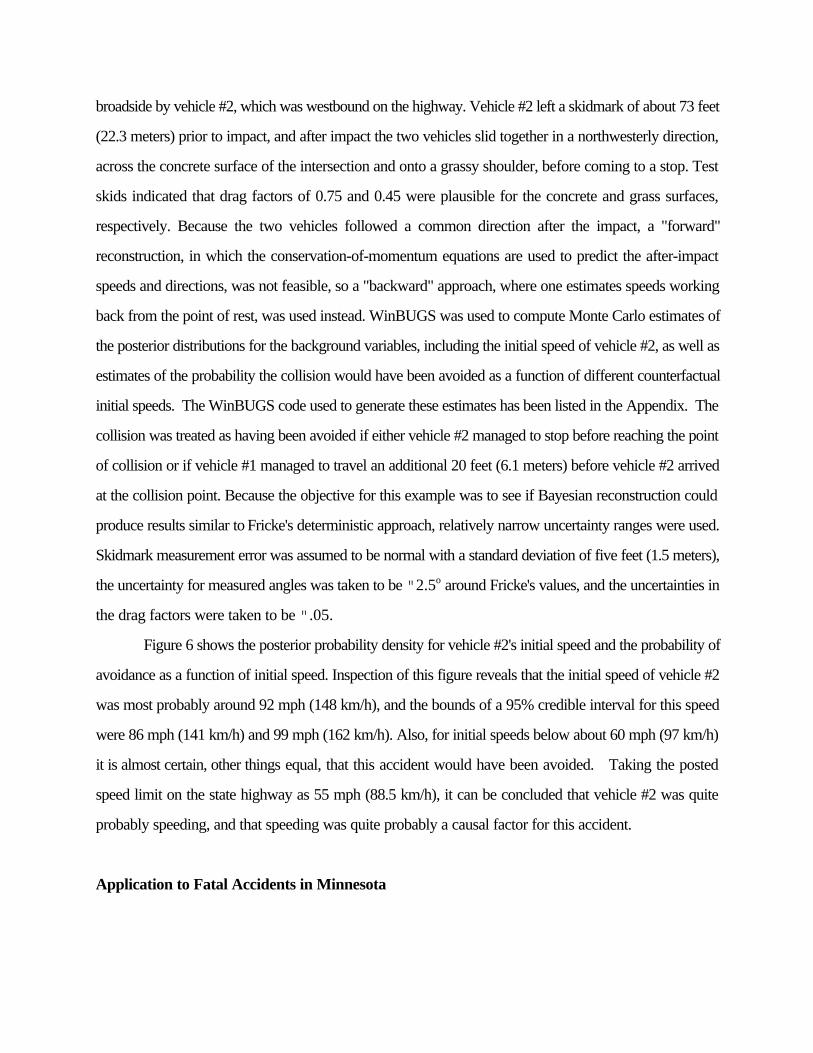
Figure 6 shows the posterior probability density for vehicle #2's initial speed and the probability of

avoidance as a function of initial speed. Inspection of this figure reveals that the initial speed of vehicle #2

was most probably around 92 mph (148 km/h), and the bounds of a 95% credible interval for this speed

were 86 mph (141 km/h) and 99 mph (162 km/h). Also, for initial speeds below about 60 mph (97 km/h)

it is almost certain, other things equal, that this accident would have been avoided. Taking the posted

speed limit on the state highway as 55 mph (88.5 km/h), it can be concluded that vehicle #2 was quite

probably speeding, and that speeding was quite probably a causal factor for this accident.

Application to Fatal Accidents in Minnesota

As part of this study, Minnesota Dept. of Transportation (MNDOT) personnel identified all fatal

accidents listed as occurring on state highways between January 1 1997 and June 30 2000 that were near

on of MNDOT's automatic speed recording stations. Visits to district offices of the Minnesota State Patrol

then produced detailed investigation information for 46 fatal accidents, and of these seven involved

collisions between motor vehicles and pedestrians while nine were multiple vehicle collisions at intersections.

For four of the pedestrian collisions and two of the intersection collisions it was possible to apply the

Bayesian network methods described above to estimate initial vehicles speeds and compute probabilities

of avoidance. The results of these computations are displayed in Figures 7-12.

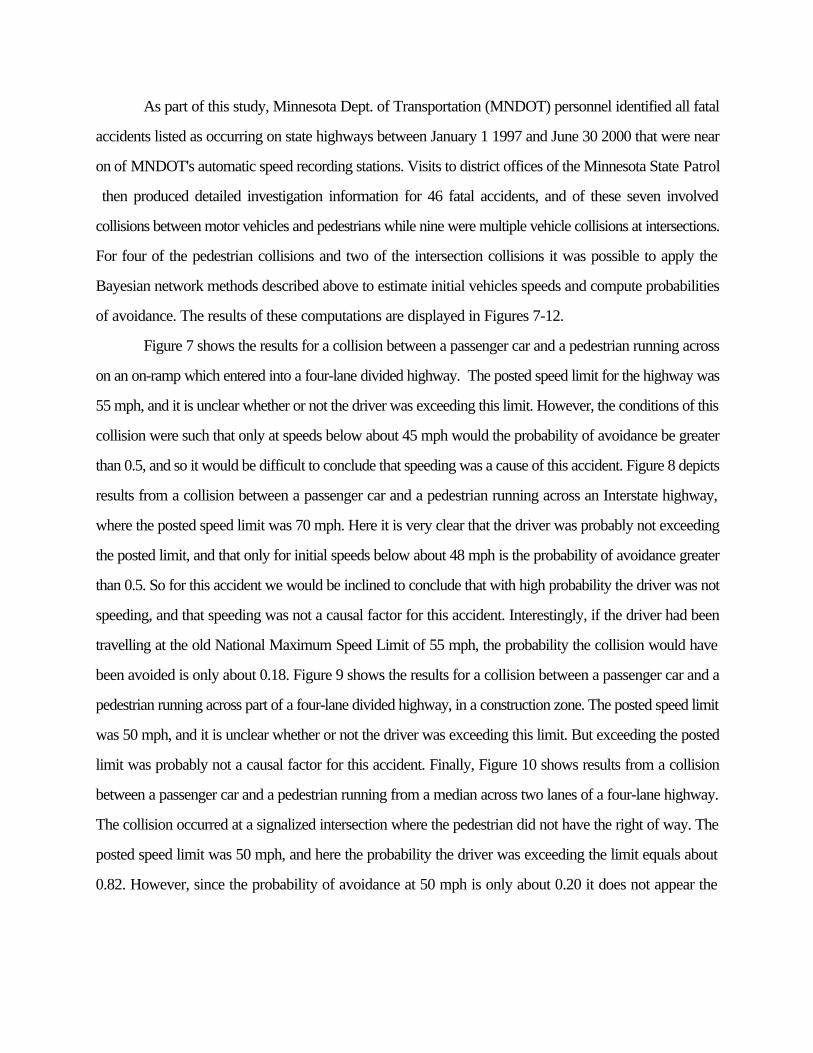
Figure 7 shows the results for a collision between a passenger car and a pedestrian running across

on an on-ramp which entered into a four-lane divided highway. The posted speed limit for the highway was

55 mph, and it is unclear whether or not the driver was exceeding this limit. However, the conditions of this

collision were such that only at speeds below about 45 mph would the probability of avoidance be greater

than 0.5, and so it would be difficult to conclude that speeding was a cause of this accident. Figure 8 depicts

results from a collision between a passenger car and a pedestrian running across an Interstate highway,

where the posted speed limit was 70 mph. Here it is very clear that the driver was probably not exceeding

the posted limit, and that only for initial speeds below about 48 mph is the probability of avoidance greater

than 0.5. So for this accident we would be inclined to conclude that with high probability the driver was not

speeding, and that speeding was not a causal factor for this accident. Interestingly, if the driver had been

travelling at the old National Maximum Speed Limit of 55 mph, the probability the collision would have

been avoided is only about 0.18. Figure 9 shows the results for a collision between a passenger car and a

pedestrian running across part of a four-lane divided highway, in a construction zone. The posted speed limit

was 50 mph, and it is unclear whether or not the driver was exceeding this limit. But exceeding the posted

limit was probably not a causal factor for this accident. Finally, Figure 10 shows results from a collision

between a passenger car and a pedestrian running from a median across two lanes of a four-lane highway.

The collision occurred at a signalized intersection where the pedestrian did not have the right of way. The

posted speed limit was 50 mph, and here the probability the driver was exceeding the limit equals about

0.82. However, since the probability of avoidance at 50 mph is only about 0.20 it does not appear the

speeding should be considered a causal factor for this accident.

Figure 11 shows results from a collision between a left-turning vehicle and an eastbound vehicle on

a four-lane county highway. The intersection was not signalized, the eastbound driver had the right-of-way,

and the posted speed limit was 55 mph. The results shown in Figure 11 are for the eastbound vehicle. Here

it is clear that the eastbound driver was not exceeding the posted limit, and in fact was probably travelling

well below the limit. Clearly, exceeding the posted limit was probably not a causal factor in this collision.

Finally, Figure 12 depicts results from a collision between two pickup trucks at a two-way stop controlled

intersection. The major street was a four-lane divided highway with a posted speed limit of 55 mph, and

the results in Figure 12 are for the major road vehicle. Here it is quite probable that the major road driver

was exceeding the posted speed limit, and the probability of avoidance at the posted limit is about 0.56.

Here it appears quite probable that the major road driver was speeding, and it is more probable than not

that speeding was a causal factor for this accident.

Conclusion

Statistical methods are now commonly used to study relationships between traffic engineering

actions and the incidence of accidents, but in Technical Report 1 we pointed out how failure to attend to

the underlying processes which generate accidents can lead to misinterpretation of statistical results. In

Technical Report 1 we alluded to Snow's work on identifying the mechanism of transmission for cholera,

which utilized both statistical and clinical methods to test hypotheses about transmission. The main objective

of the work described in this report was to develop and apply a method for using clinical investigations of

road accidents to support and inform traffic engineering decisions. The basic idea is straightforward: if the

oft-reported statistical associations between average speed, or changes in speed limits, and the occurrence

of fatal and serious road accidents reflect a causal connection, then it ought to be possible to identify speed

as a causal factor in at least a substantial fraction of actually occurring accidents. Implementing this idea is

bit more difficult however, and our general approach has been adapt ideas from formal logic and artificial

intelligence in order to specify truth conditions for causal claims, and then use probability theory to assess

the degree to which evidence supports or contradicts those claims. This leads to what is essentially a

Bayesian network approach to doing traffic accident reconstruction, and in this report we developed some

of the connections between accident reconstruction, forensic inference, and probabilistic reasoning.

Our Bayesian network approach was applied to ten actual accidents involving either collisions

between vehicles and pedestrians or collisions between vehicles at intersections. Three of the

vehicle/pedestrian collision occurred on lower speed roads, and in two of these it appeared both that the

vehicle was probably speeding prior to the collision and that speeding could be considered a causal factor

for these collisions. In the third low-speed road collision it was unclear whether or not the driver was

speeding but speeding probably was not a causal factor. The other four pedestrian collisions occurred on

higher speed roads in Minnesota, and in each the conditions were such that the driver had the right of way.

In three of the four it was not obvious that the driver was speeding, and speeding could not be considered

a causal factor, while in the fourth it did appear that the driver was speeding but speeding still could not

be considered a causal factor. When considering the two-vehicle intersection collisions, all three occurred

on higher speed roads, and in two it was clear that the vehicle with the right-of-way speeding, and that

speeding was probably a causal factor for these collisions. In the third intersection collision it was clear the

right-of-way vehicle was not speeding and that speeding was not a causal factor.

With the exception of Fricke's (1990) example collision, it does not appear that the vehicles

involved in these collisions were travelling at exceptionally high speeds, and it seems reasonable to suspect

that other drivers traversed the accident scene at about the same time as fast or even faster without being

involved in collisions. This in turn suggests that speeding by itself is not sufficient to cause a crash, nor does

it appear to be necessary. Rather, for these crashes it appears that first an accident avoidance situation is

triggered, by a pedestrian or other vehicle attempting to cross an oncoming vehicle's path, and then speed

interacts with the other characteristics of that particular situation to determine whether or not the crash

occurs. The focus of this report has been on determining whether or not speeding should be considered a

causal factor in road accidents, and causal factors are analogous to what Pearl (2000) calls necessary

causes, since their absence is sufficient to prevent the accident. Road accidents usually result though from

a particular combination of several causal factors, none of which was sufficient in and of itself to produce

the accident. An intriguing extension of this Bayesian approach would be toward identifying what Baker

calls the cause of an accident, that is, the complete set of causal factors which, if reproduced, would result

in an identical accident (1975, p. 284).

Finally, the tentative conclusions advanced in this report apply only to the types of accidents

considered here. Single vehicle run-off road accidents will be considered in Technical Report 3.

References

Aitken, C. Connolly, T. Gammerman, A. Zhang, G., Bailey, D., Gordon, R., & Oldfield, R. 1996 Statisticalmodeling in specific case analysis. Science and Justice. 36, 245-255.

Bacchus, F. 1990 Representing and Reasoning with Probabilistic Knowledge. Cambridge, MA, MITPress.

Baker, J. 1975 Traffic Accident Investigation Manual. Evanston, IL, Northwestern University TrafficInstitute.

Baker, J. & Fricke, L. 1990 Process of traffic accident reconstruction. Traffic Accident Reconstruction(L. Fricke, ed.) Evanston, IL, Northwestern University Traffic Institute.

Balding, D. Interpreting DNA evidence: Can probability theory help? Statistical Science in theCourtroom (J. Gastwirth, ed.) New York, Springer, 51-70.

Balke, A.,& Pearl, J. 1994 Probabilistic evaluation of counterfactual queries. Proceedings of 12thNational Conference on Artificial Intelligence, Menlo Park, NJ, AAAI Press, 230-237.

Brach, R. 1994 Uncertainty in accident reconstruction calculation. Accident Reconstruction: Technologyand Animation IV, Warrendale, PA, SAE Inc, 147-153.

Carnap, R. 1945 The two concepts of probability. Philosophy and Phenomenological Research. 5, 513-532.

Carnap, R. 1971 A basic system of inductive logic, part I. Studies in Inductive Logic and Probability,vol. I. (R. Carnap & R. Jeffrey, eds.) Berkeley, CA, Univ of California Press, 33-166.

Curran, J., Triggs, C., Buckleton, J., Walsh, K., & Hicks, T. 1998 Assessing transfer probabilities in aBayesian interpretation of forensic glass evidence. Science and Justice. 38, 15-21.

Davis, G. 1999 Using graphical Markov models and Gibbs sampling to reconstruct vehicle/pedestrianaccidents. Proceedings of the Conference Traffic Safety on Two Continents. Linkoping,Sweden, Swedish National Road and Transport Research Institute.

Davis, G. 2001 Using Bayesian networks to identify the causal effect of speeding in individualvehicle/pedestrian collisions. Proceedings of the 17th Conference on Uncertainty in ArtificialIntelligence, (J. Breese & D. Koller, eds.) San Francisco, Morgan Kaufmann, 105-111.

Davis, G., Sanderson, K., & Davuluri, S. 2002 Development and Testing of a Vehicle/PedestrianCollision Model for Neighborhood Traffic Control. Report 2002-23, St. Paul, MN, Minnesota

Dept. of Transportation. Dawid, A., & Evett, I. 1997 Using a graphical method to assist the evaluation of complicated patterns of

evidence. Journal of Forensic Science, 42, 226-231.Dawid, P. & Mortera, J. 1998 Forensic identification with imperfect evidence. Biometrika, 85, 835-849.Dubois, D. & Prade, H. 1993 A glance at non-standard models and logics of uncertainty and vagueness.

Philosophy of Probability, (J-P Dubucs, ed.) Dordrecht, Kluwer, 169-222.Earman, J. 1992 Bayes or Bust? Cambridge, MA, MIT Press.Edwards, W. 1991 Influence diagrams, Bayesian imperialism, and the Collins case: An appeal to reason.

Cardozo Law Review. 13, 1025-1079.Eubanks, J., & Hill, P.1998 Pedestrian Accident Reconstruction and Litigation. Tuscon, AZ, Lawyers

and Judges Publishing Co.Fambro, D., Koppa, R., Picha, D., & Fitzpatrick, K. 1998 Driver perception-brake response in stopping

sight distance situations. paper 981410 presented at 78th Annual Meeting of TransportationResearch Board, Washington, DC.

Fricke, L. (1990) Traffic Accident Reconstruction, Traffic Institute, Northwestern University, EvanstonIL.

Garrott, W., & Guenther, D. 1982 Determination of precrash parameters from skid mark analysis.Transportation Research Record, 893, 38-46.

Greatrix, G. 2002 AI lecture notes 2: Analysis of a simple accident. Accident Investigation LectureNotes, World Wide Website http://scratchy.spods.co.uk/~greatrix/AINotes.html, December 27,2002.

Hacking, I. 1965 The Logic of Statistical Inference. Cambridge, UK, Cambridge Univ. Press.Hacking, I. 1975 The Emergence of Probability. Cambridge, UK, Cambridge Univ. Press.Halpern, J. 1990 An analysis of first-order logics of probability. Artificial Intelligence, 46, 311-350.Hicks, J. 1989 Traffic accident reconstruction. Forensic Engineering. (K. Carper, ed.) New York,

Elsevier, 101-129.Hoogstrate, A. & Spek, A. 2002 Monte Carlo simulation and inference in accident reconstruction.

presented at 5th International Conference on Forensic Statistics, Venice.Howson, C. 1993 Personalistic Bayesianism. Philosophy of Probability. (J-P Dubucs, ed.) Dordrecht,

Kluwer, 1-12.Jensen, F. 1996 An Introduction to Bayesian Networks. New York, Springer.Kost, G. & Werner, S. 1994 Use of Monte Carlo simulation techniques in accident reconstruction. SAE

Technical Paper 940719, Warrendale, PA, SAE, Inc.Lewis, D. 1973 Counterfactuals. Oxford, UK, Blackwell.Lewis, D. 1976 Probabilities of conditionals and conditional probabilities. Philosophical Review. 85, 297-

315.Lewis, D. 1980 A subjectivist’s guide to objective chance. Studies in Inductive Logic and Probability,

v. II, (R. Jeffrey, ed.) Berkeley, CA, Univ. California Press, 263-294.Limpert, R. 1989 Motor Vehicle Accident Reconstruction and Cause Analysis. 3rd ed. Charlottesville,

VA, Michie Co.Lindley, D. 1991 Subjective probability, decision analysis and their legal consequences. Journal of Royal

Statistical Society A, 154, 83-92.McLean, J., Anderson, R., Farmer, M., Lee, B., and Brooks, C. 1994 Vehicle Travel Speeds and the

Incidence of Fatal Pedestrian Crashes, Road Accident Research Unit, University of Adelaide,Adelaide, AU.

NCUTLO 1992 Uniform Vehicle Code and Model Traffic Ordinance, National Committee on UniformLaws and Ordinances, Evanston, IL.

Neptune, J., Flynn, J., Chavez, P., & Underwood, H. 1995 Speed from skids: A modern approach.Accident Reconstruction: Technology and Animation V. Warrendale, PA, SAE, Inc, 189-204.

Niederer, P. 1991 The accuracy and reliability of accident reconstruction. Automotive Engineering andLitigation. vol. 4, (G. Peters and G. Peters, eds.) New York, Wiley and Sons, 257-303.

Pearl, J. 2000 Causality: Models, Reasoning, and Inference. Cambridge, UK, Cambridge UniversityPress.

Poole, D. & Raftery, A. 2000 Inference for deterministic simulation models: The Bayesian meldingapproach. Journal of American Statistical Association. 95,1244-1255.

Reed, W. & Keskin, A. 1989 Vehicular deceleration and its relationship to friction. SAE Technical Paper890736. Warrendale, PA, SAE, Inc.

Road Traffic Act 1991, Her Majesty's Stationery Office, London, UK.Rose, N. Fenton, S. & Hughes, C. 2001 Integrating Monte Carlo simulation, momentum-based impact

modeling, and restitution data to analyze crash severity. SAE Technical Paper 2001-01-3347,Warrendale, PA, SAE Inc.

Rudram, D. & Lambourn, R. 1981 The scientific investigation of road accidents. Journal of OccupationalAccidents, 3 177-185.

Schockenhoff, G. Appel, H. & Rau, H. 1985 Representation of actual reconstruction methods for car-to-car accidents as confirmed by crash tests. SAE Technical Paper 850066, Warrendale, PA, SAEInc.

Schum, D. 2000 Singular evidence and probabilistic reasoning in judicial proof. Harmonisation inForensic Expertise (J. Nijboer & W. Sprangers, eds.) Thela Thesis, 587-603.

Spiegelhalter, D., Thomas, A., & Best, N. 2000 WinBUGS Version 1.3 User Manual. Oxford, UK,MRC Biostatistics Unit, Oxford University.

Stalnaker, R. 1968 A theory of conditionals. American Philosophical Monograph Series #2, (N.Rescher, ed.) Oxford, UK, Blackwell.

Stewart-Morris, M. 1995 Real time, accurate recall, and other myths. Forensic Accident Investigation:Motor Vehicles. (T. Bohan & A. Damask, eds.) Charlottesville, VA, Michie Butterworth, 413-438.

Traffic Institute 1946 Accident Investigation Manual. Evanston, IL, Northwestern University TrafficInstitute.

Wood, D. & O’Riordain, S. 1994 Monte Carlo simulation methods applied to accident reconstruction andavoidance analysis. Accident Reconstruction: Technology and Animation IV. Warrendale, PA,SAE Inc, 129-136.

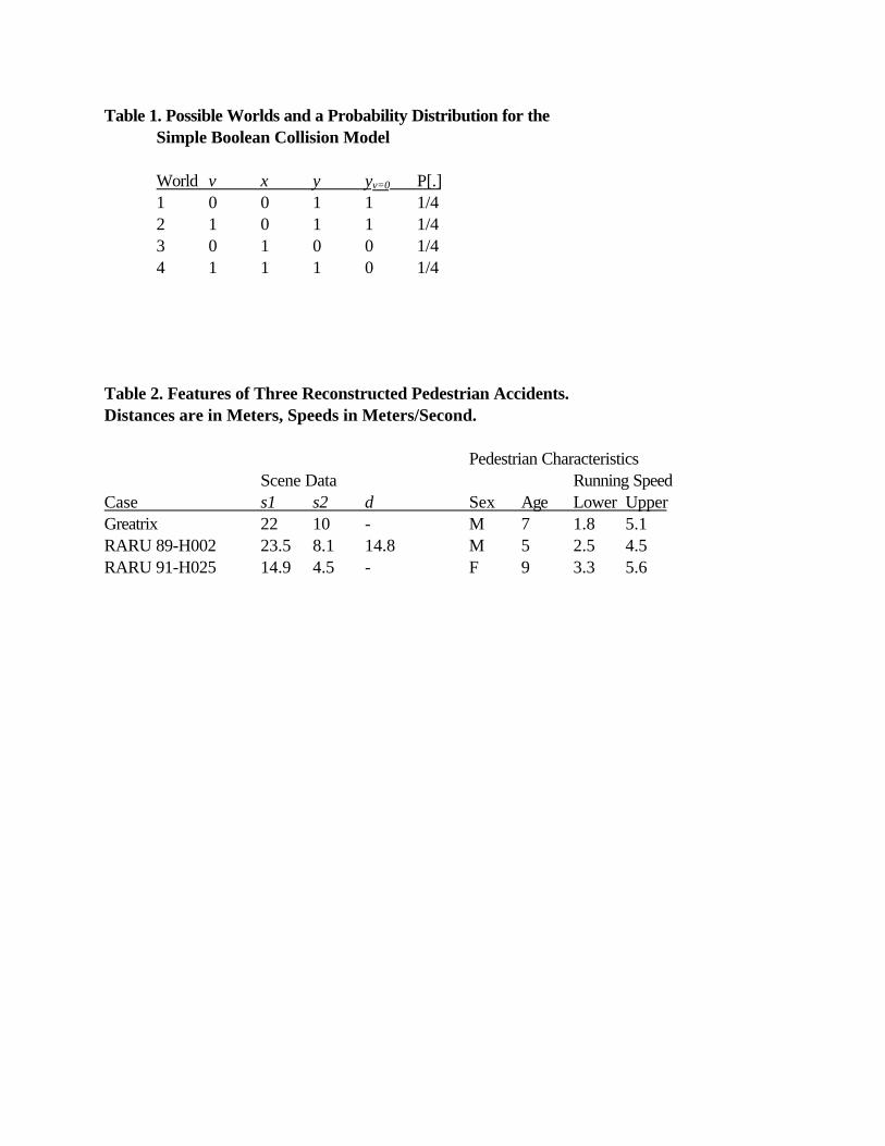
Table 1. Possible Worlds and a Probability Distribution for theSimple Boolean Collision Model

World v x y yv=0 P[.]1 0 0 1 1 1/42 1 0 1 1 1/43 0 1 0 0 1/44 1 1 1 0 1/4

Table 2. Features of Three Reconstructed Pedestrian Accidents.Distances are in Meters, Speeds in Meters/Second.

Pedestrian CharacteristicsScene Data Running Speed

Case s1 s2 d Sex Age Lower UpperGreatrix 22 10 - M 7 1.8 5.1RARU 89-H002 23.5 8.1 14.8 M 5 2.5 4.5RARU 91-H025 14.9 4.5 - F 9 3.3 5.6

Figure 1. Major Variables Appearing in the Vehicle/Pedestrian Collision Model.

x

d

xsvtp s1

s2

Figure 2. Directed Acyclic Graph Representation of Vehicle/Pedestrian Collision Model.

x v f

vid

s1

s2

tp tsx f

vid

s1

s2

tp ts v

v2

y*

v*

Figure 3. Posterior Density for Vehicle's Initial Speed, and Probability of Avoidance as a Functionof Initial Speed: Greatrix's Example.

15 20 25 30 35 40 45 50 55 600

0.2

0.4

0.6

0.8

1

P[v | y=1&e]PA(v)

Speed (mph)

Prob

abili

ties

1.1

0

p1 i

pdr i

59.04318.645 speedmph i

Figure 4. Posterior Density for Vehicle's Initial Speed, and Probability of Avoidance as a Functionof Initial Speed: RARU Case 89-H002.

30 40 50 60 70 80 90 1000

0.2

0.4

0.6

0.8

1

P[v | y=1&e]PA(v)

Speed (kph)

Prob

abili

ties

1.1

0

p1 i

pdr i

9530 speedkph i

Figure 5. Posterior Density for Vehicle's Initial Speed, and Probability of Avoidance as a Functionof Initial Speed: RARU Case 91-H025.

30 40 50 60 70 80 90 1000

0.2

0.4

0.6

0.8

1

P[v | y=1&e]PA(v)

Speed (kph)

Prob

abili

ties

1.1

0

p1 i

pdr i

9530 speedkph i

Figure 6. Posterior Density for Vehicle's Initial Speed, and Probability of Avoidance as a Functionof Initial Speed: Vehicle 2 in Fricke 1990 Two-Vehicle Example.

40 60 80 100 120 1400

0.2

0.4

0.6

0.8

1

P[v | y=1&e]PA(v)

Speed (mph)

Prob

abili

ties

1.1

0

p1 i

pdr i

14050 speedmph i

Figure 7. Posterior Distribution for Vehicle's Initial Speed, and Probability of Avoidance, for aVehicle/Pedestrian Collision at On-Ramp onto USTH 52 in Rochester. Posted Speed Limit onHighway was 55 mph.

20 25 30 35 40 45 50 55 60 65 70 75 800

0.1

0.2

0.3

0.4

0.5

0.6

0.7

0.8

0.9

1

1.1

P[v | y=1&e]PA(v)

Speed (mph)

Prob

abili

ties

1.1

0

p1i

pdri

71.324.8 speedkphi .62⋅

Figure 8. Posterior Distribution for Vehicle's Initial Speed, and Probability of Avoidance, for aVehicle/Pedestrian Collision on Northbound ISTH 35W. Posted Speed Limit on Highway was 70mph.

20 25 30 35 40 45 50 55 60 65 70 75 80 85 900

0.1

0.2

0.3

0.4

0.5

0.6

0.7

0.8

0.9

1

1.1

P[v | y=1&e]PA(v)

Speed (mph)

Prob

abili

ties

1.1

0

p1i

pdri

80.624.8 speedkphi .62⋅

Figure 9. Posterior Distribution for Vehicle's Initial Speed, and Probability of Avoidance, for aVehicle/Pedestrian Collision at Northbound USTH 61, in Newport. Posted Speed Limit onHighway was 50 mph.

20 25 30 35 40 45 50 55 60 65 70 75 800

0.1

0.2

0.3

0.4

0.5

0.6

0.7

0.8

0.9

1

1.1

P[v | y=1&e]PA(v)

Speed (mph)

Prob

abili

ties

1.1

0

p1i

pdri

71.324.8 speedkphi .62⋅

Figure 10. Posterior Distribution for Vehicle's Initial Speed, and Probability of Avoidance, for aVehicle/Pedestrian Collision on Westbound MNTH 36, in Stillwater. Posted Speed Limit onHighway was 50 mph.

20 25 30 35 40 45 50 55 60 65 70 75 800

0.1

0.2

0.3

0.4

0.5

0.6

0.7

0.8

0.9

1

1.1

P[v | y=1&e]PA(v)

Speed (mph)

Prob

abili

ties

1.1

0

p1i

pdri

71.324.8 speedkphi .62⋅

Figure 11. Posterior Distribution for Vehicle's Initial Speed, and Probability of Avoidance, forMajor-Road Vehicle in Two-Vehicle Collision on Anoka CSAH 23. Posted Speed Limit onHighway was 55 mph.

20 25 30 35 40 45 50 55 60 65 70 75 80 85 900

0.1

0.2

0.3

0.4

0.5

0.6

0.7

0.8

0.9

1

1.1

P[v | y=1&e]PA(v)

Speed (mph)

Prob

abili

ties

1.1

0

p1i

pdri

9020 speedmphi

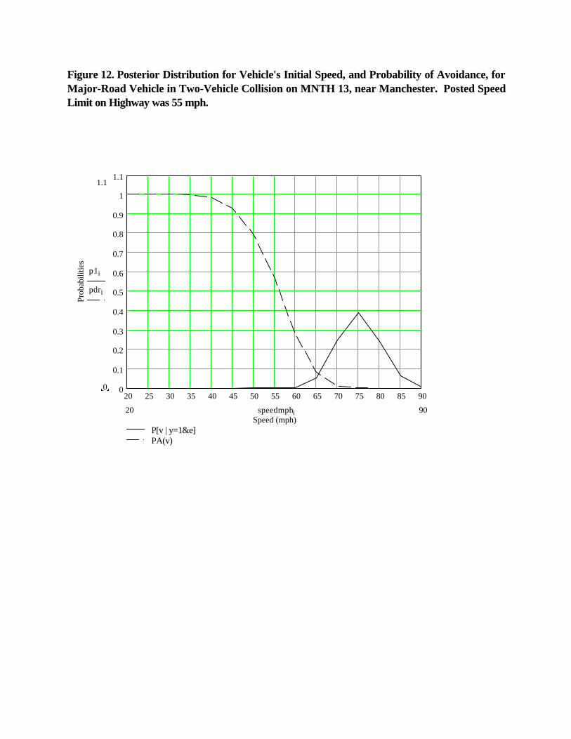
Figure 12. Posterior Distribution for Vehicle's Initial Speed, and Probability of Avoidance, forMajor-Road Vehicle in Two-Vehicle Collision on MNTH 13, near Manchester. Posted SpeedLimit on Highway was 55 mph.

20 25 30 35 40 45 50 55 60 65 70 75 80 85 900

0.1

0.2

0.3

0.4

0.5

0.6

0.7

0.8

0.9

1

1.1

P[v | y=1&e]PA(v)

Speed (mph)

Prob

abili

ties

1.1

0

p1i

pdri

9020 speedmphi

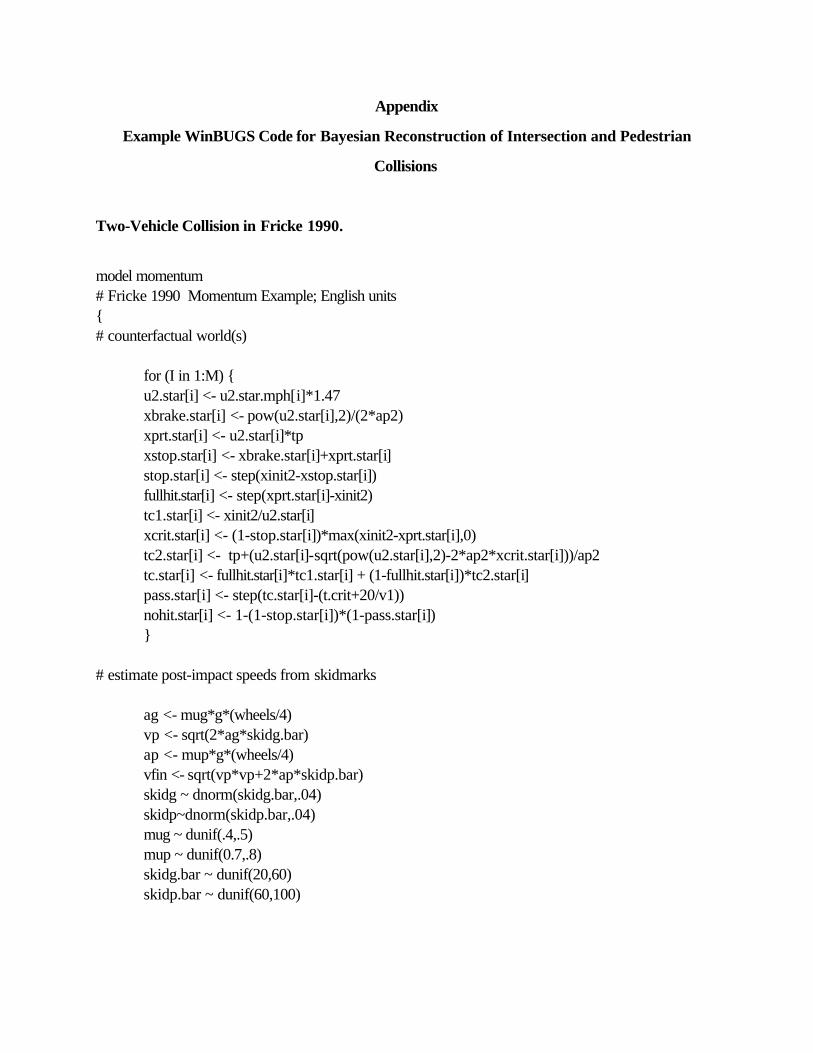
Appendix

Example WinBUGS Code for Bayesian Reconstruction of Intersection and Pedestrian

Collisions

Two-Vehicle Collision in Fricke 1990.

model momentum# Fricke 1990 Momentum Example; English units{# counterfactual world(s)

for (I in 1:M) {u2.star[i] <- u2.star.mph[i]*1.47xbrake.star[i] <- pow(u2.star[i],2)/(2*ap2)xprt.star[i] <- u2.star[i]*tpxstop.star[i] <- xbrake.star[i]+xprt.star[i]stop.star[i] <- step(xinit2-xstop.star[i])fullhit.star[i] <- step(xprt.star[i]-xinit2)tc1.star[i] <- xinit2/u2.star[i]xcrit.star[i] <- (1-stop.star[i])*max(xinit2-xprt.star[i],0)tc2.star[i] <- tp+(u2.star[i]-sqrt(pow(u2.star[i],2)-2*ap2*xcrit.star[i]))/ap2tc.star[i] <- fullhit.star[i]*tc1.star[i] + (1-fullhit.star[i])*tc2.star[i]pass.star[i] <- step(tc.star[i]-(t.crit+20/v1))nohit.star[i] <- 1-(1-stop.star[i])*(1-pass.star[i])}

# estimate post-impact speeds from skidmarks

ag <- mug*g*(wheels/4)vp <- sqrt(2*ag*skidg.bar)ap <- mup*g*(wheels/4)vfin <- sqrt(vp*vp+2*ap*skidp.bar)skidg ~ dnorm(skidg.bar,.04)skidp~dnorm(skidp.bar,.04)mug ~ dunif(.4,.5)

mup ~ dunif(0.7,.8) skidg.bar ~ dunif(20,60) skidp.bar ~ dunif(60,100)

# estimate pre-impact speeds using momentum conservation

m1 <- wcar1m2 <- wcar2

alpha1 ~ dunif(a1low,a1up)alpha2 ~ dunif(a2low,a2up)beta ~ dunif(blow,bup)

c <- 3.141592/180

v2 <- (vfin*m1*sin(beta*c)+vfin*m2*sin(beta*c))/(m2*sin(alpha2*c))v1<-(vfin*m1*cos(beta*c)+vfin*m2*cos(beta*c)-v2*m2*cos(alpha2*c))/(m1*cos(alpha1*c))

# estimate vehicle 2 initial speed and distance

ap2 <- mup*gxx <- max(0,x)u2 <- sqrt((v2*v2+2*ap2*xx))x.tran2 <- u2*ts-(ap2*pow(ts,2))/2x.prt <- tp*u2

skid21.bar <- x-x.tran2 skid21 ~ dnorm(skid21.bar,.04)

xinit2 <-x+x.prtlimit.fps <- limit*1.47speeding <- step(u2-limit.fps)

# estimate vehicle 1's initial speed and critical time

notime <- step(-x.prt-x)fullhit <- step(-x)littletime <- step(-x)*(1-notime)

t.crit <- 0*notime+littletime*(tp+(x/u2))+(1-fullhit)*(tp+((u2-v2)/ap2))temp <- step(v1*v1-2*a1*xinit1)u1 <- sqrt(temp*(v1*v1-2*a1*xinit1))

a1 ~ dunif(0,8)

tp ~ dunif(0.5, 2.5)ts ~ dunif(.1,.5)x ~ dunif(-10,150)

u1.mph <- u1/1.47u2.mph <- u2/1.47v1.mph <- v1/1.47v2.mph <- v2/1.47

}

Data list(g=32.2, skidg=40, skidp=80,wcar1=3600,wcar2=3700,skid21=73,xinit1=53,a1low=-2.5,a1up=2.5, a2low=272.5, a2up=277.5, blow=287.5, bup=292.5,wheels=3, limit=55,M=15,u2.star.mph=c(40,45,50,55,60,65,70,75,80,85,90,95,100,105,110))

Inits list(mup=0.75, mug=.45,alpha1=0, alpha2=275, beta=290 )

Vehicle Pedestrian Collision Depicted in Figure 10.

model pedmodel# Case #98409793# includes counterfactual injury model# damage model parameters taken from MNDOT report: Davis, Sanderson and Davuluri (2002)# metric units{

# counterfactual worldfor (i in 1:M) { v.star[i] <- v.star.kph[i]/3.6; xbrake.star[i] <- pow(v.star[i],2)/(2*a); xprt.star[i] <- v.star[i]*tp; xstop.star[i] <- xbrake.star[i] + xprt.star[i] stop.star[i] <- step(x.init-xstop.star[i]); fullhit.star[i] <- step(xprt.star[i]-x.init); tc1.star[i] <- x.init/v.star[i]; xcrit.star[i] <- (1-stop.star[i])*max(x.init-xprt.star[i],0) tc2.star[i] <-tp+(v.star[i]-sqrt(pow(v.star[i],2)-2*a*xcrit.star[i]))/a; tc.star[i] <- fullhit.star[i]*tc1.star[i] + (1-fullhit.star[i])*tc2.star[i]; pass.star[i] <- step(tc.star[i]-(t.ped+t.buffer)); nohit.star[i] <- 1-(1-stop.star[i])*(1-pass.star[i])

v2.imp.star[i] <- fullhit.star[i]*pow(v.star[i],2) +

(1-fullhit.star[i])*(pow(v.star[i],2)-2*a*(max(0,x.init-xprt.star[i]))) vi.kph.star[i] <-3.6* sqrt(max(0,v2.imp.star[i])); damage.star[i] <- b*vi.kph.star[i] + randam slight.star[i] <- step(a1-damage.star[i])*(1-nohit.star[i]) serious.star[i] <- step(damage.star[i]-a1)*step(a2-damage.star[i])*(1-nohit.star[i]) fatal.star[i] <- step(damage.star[i]-a2)*(1-nohit.star[i]) }

# data models

dam.bar <- b*vi.kphrandam ~ dlogis(0,1)damage <- dam.bar+randamslight <- step(a1-damage)serious <- step(damage-a1)*step(a2-damage)fatal <- step(damage-a2)psev[1] <- .999*slight+.001/3psev[2] <- .999*serious+.001/3psev[3] <- .999*fatal+.001/3injury ~ dcat(psev[])

throw.bar <- ahat+2*log(vi); throw.tau <- 1/(throw.sig2); throw ~ dnorm(throw.bar,throw.tau); skid1.bar <- max(0.1,x.brake-x.tran); lvi <- max(0.1,log(vi)); logskid1.bar <- log(skid1.bar); logskid2.bar <- 2*lvi-log(2*a);# skid2.bar <- pow(vi,2)/(2*a); skid1 ~ dnorm(logskid1.bar,skid.tau); skid2 ~ dnorm(logskid2.bar,skid.tau);

# braking model a <- f*(9.807); x.brake <- pow(v,2)/(2*a); x.tran <- v*ts-(a*pow(ts,2))/2; x.prt <- v*tp; xx <- max(x,-x.prt); nohit <- step(x-x.brake);

fullhit <- step(-x); skidmark <- step(x.brake-x.tran); v2.imp <- (1-nohit)*((fullhit*pow(v,2)) + (1-fullhit)*(pow(v,2)-2*a*(max(0,x)))); vi <- sqrt(v2.imp); x.init <- xx + x.prt; notime <- step(-x.prt-x); littletime <- step(-x)*(1-notime); t.ped <- 0*notime+littletime*(tp+x/v)+(1-fullhit)*(tp+(v-vi)/a); vi.kph <- (3.6)*vi; v.kph <- (3.6)*v; speeding <- step(v-v.limit); t.buffer <- clear/ped.speed;

# prior distributions tp ~ dunif(tp.lower,tp.upper); ts ~ dunif(ts.lower,ts.upper); x ~ dunif(x.lower, x.upper); v ~ dunif(v.lower, v.upper); f ~ dunif(f.lower, f.upper);

a1.tau <- 1/(a1.sig*a1.sig)a2.tau <- 1/(a2.sig*a2.sig)b.tau <- 1/(b.sig*b.sig)

a1~dnorm(a1.bar,a1.tau)I(,a2) a2~dnorm(a2.bar,a2.tau)I(a1,) b~dnorm(b.bar,b.tau)

# speed.tau <- 1/(speed.sig*speed.sig); # speed.mph ~dnorm(speed.bar.mph,speed.tau); # speed.kph <- speed.mph*1.609; ped.speed ~ dunif(ped.lower,ped.upper);}

Data list(M=17,skid1=3.58,skid2=3.07,throw=3.19,injury=3,a1.bar=4.97,a1.sig=.531,a2.bar=8.87,

a2.sig=.822b.bar=0.127,b.sig=.018,v.lower=10,v.upper=45;f.lower=0.55,f.upper=0.9,x.lower=0,x.upper=60,ts.lower=0.1,ts.upper=0.5,tp.lower=0.5,tp.upper=2.5,ahat=-2.24,throw.sig2 = 0.084,skid.tau= 100,v.limit=22.35,ped.lower=1.0,ped.upper=4.5,clear=3.0,v.star.kph=c(40,45,50,55,60,65,70,75,80,85,90,95,100,105,110,115,120))

Inits list(tp=1.5,x=12,v=15,f=.73,ts=.3,randam=0,a1=4.9,a2=8.7,b=.12)