A BRKGA for the project scheduling problem withflexible resources

Bernardo F. Almeidaa∗, Isabel Correiab, Francisco Saldanha-da-Gamaa

a Departamento de Estatıstica e Investigacao Operacional / Centro de Matematica e AplicacoesFundamentais — Centro de Investigacao Operacional, Faculdade de Ciencias, Universidade Lisboa,

1749-016 Lisboa, Portugalb Departamento de Matematica / Centro de Matematica e Aplicacoes, Faculdade de Ciencias e

Tecnologia, Universidade Nova Lisboa, 2829-516 Caparica, Portugal

Abstract

In this paper we address a project scheduling problem with flexible resources. ThisNP-Hard combinatorial optimization problem is associated with scheduling a set ofactivities which require specific resource units for each one of the several skills neededfor their execution, such that the makespan of the project is minimized. We proposea biased random-key genetic algorithm (BRKGA) for computing feasible solutions forthe referred problem. We study different decoding mechanisms: heuristic of Almeidaet al. (2016), a new adapted serial scheduling generation scheme and both. TheBRKGA is tested on a total of 432 instances of different dimensions and the resultsindicate that the developed algorithm is robust and attains high quality solutions.

Keywords: Project scheduling, Flexible resources, Biased random-key genetic algo-rithm.

∗Corresponding author. e-mail address: bernardo.almeida@alunos.fc.ul.pt

1

1 Introduction

In the classical resource-constrained project scheduling problem (RCPSP) a set of time

dependent activities which require specific resources that are available in limited quantities,

has to be scheduled such that the makespan of the project is minimized. This problem has

been widely studied in the literature along with many variants of it due to their associated

large number of real-world applications (for overviews the reader should refer to the work

of Herroelen and Demeulemeester (1998), Brucker et al. (1999), Hartmann and Briskorn

(2010), Weglarz et al. (2011), and the references therein).

In many resource constrained project scheduling problems, resources are flexible mean-

ing that each resource often performs more than one skill. This situation usually arises

when human resources or multi-purpose machines are involved in the project. Typically

in this context, activities require specific resource units of several skills to be processed.

The assignment of a resource to an activity comprehends the decision of the skill it will

perform, from the set of skills required by that activity and mastered by this resource.

The problem we have just described falls into the class of project scheduling problems

with flexible resources (PSPFR) which consists of an extension of the RCPSP.

Some types of PSPFR have already been proposed in the literature. Li and Womer

(2009) study a project scheduling problem with flexible resources where each activity re-

quires only one resource unit per each skill needed for its execution. The objective function

of this problem regards the minimization of the fixed costs associated with the resources.

In a paper by Correia et al. (2012) a makespan minimization project scheduling problem

with flexible resources is studied. A variant of this problem which includes fixed and vari-

able costs for the resources was considered in Correia and Saldanha-da-Gama (2014). More

recently, Correia and Saldanha-da-Gama (2015) proposed a general modeling framework

for project staffing and scheduling problems. In multi-project problems, flexible resources

have also been considered but with additional assumptions. For example, the works of

Gutjahr et al. (2008), and Heimerl and Kolisch (2010) consider that no sequence decisions

have to be made.

The problem addressed in this paper is the project scheduling problem with flexible

resources studied by Correia et al. (2012). The authors proposed a mixed-integer linear

programming formulation together with a set of additional inequalities which was developed

with the objective of strengthen the model. The computational experience showed that,

2

as expected, due to the NP-Hard nature of the problem, this framework turned to be

effective only for small sized instances. As the development of good heuristics is necessary

to compute feasible solutions for larger sized instances, Almeida et al. (2016) proposed a

parallel scheduling generation scheme for this problem. With the objective of improving

the upper bounds provided by this constructive heuristic, we propose in this paper a biased

random-key genetic algorithm (BRKGA) for the project scheduling problem with flexible

resources. A BRKGA is a population based metaheuristic, proposed by Goncalves and

Resende (2011), where each individual is represented by an array of real numbers between

0 and 1. This method has many similarities with the classical genetic algorithms but it

uses some different strategies which aim at overcoming some of the drawbacks associated

with the genetic algorithms.

To the best of the authors’ knowledge, a BRKGA has never been proposed for a

project scheduling problem with flexible resources although it has been applied to resource-

constrained project scheduling problems (Goncalves et al. 2008, Mendes et al. 2009, Goncalves

et al. 2011). BRKGA algorithms have also been successfully applied to other optimization

problems such as packing (Goncalves and Resende 2013), facility layout (Goncalves and

Resende 2015), capacitated minimum spanning trees (Ruiz et al. 2015), among others.

This paper is organized as follows. In Section 2 the PSPFR being tackled is described,

the parallel scheduling scheme studied by Almeida et al. (2016) is revisited and a serial

scheduling generation scheme is proposed. In Section 3 we review all the issues related

with the design of a generic BRKGA. Section 4 presents the BRKGA we propose for the

PSPFR. Section 5 reports the computational experience on different instance sets. Finally

our concluding remarks and directions for future work appear in Section 6.

2 PSPFR

The problem addressed in this paper is the project scheduling problem with flexible

resources (PSPFR) studied by Correia et al. (2012). In this section we define the problem

and discuss several issues related to the computation of feasible solutions.

2.1 Problem definition

The PSPFR considers a project defined by an activity-on-node network G = (V,E)

where V = {0, 1, . . . , i, j, . . . , n + 1} denotes the set of activities and the set of arcs E

3

represents the precedence relations between such activities. Activities 0 and n + 1 are

dummy activities that represent, respectively and begin and the end of the project. An

arc (i, j) belongs to E if activity i is a direct predecessor of activity j which implies that

the latter can only start after activity i has finished. The weight of each arc (i, j) is pi, the

processing time of activity i. No preemption is allowed meaning that once an activity starts

to be executed it can not be interrupted. This problem also requires a set of renewable

resources R = {1, . . . , k, . . . , K} and a set of skills L = {1, . . . , l, . . . , L}. Each resource k

has a set of skills or abilities it can perform Lk, and each activity j is associated with a

set of skills Lj which are required for performing this activity. The number of resources

required by activity j for processing skill l ∈ Lj during all its execution time is denoted

by rjl. A resource k can only be involved in one activity at a time and once it is assigned

to an activity j for performing a skill l ∈ Lj

⋂Lk, it remains assigned to that activity

performing that same skill during its whole processing time.

The objective of the PSPFR is to determine for each activity, its starting time and the

set of resources which should be assigned to each skill required for its execution, so that

the makespan is minimized, i.e, the project finishes as soon as possible.

In this problem it is also assumed that the parameters pj (j ∈ V \ {0, n + 1}) and rjl

(j ∈ V \ {0, n+ 1}; l ∈ Lj) are positive integers and are zero for the dummy activities.

From the previous data it is obvious to conclude that the makespan must be a positive

value less or equal than∑

j∈V pj (this value is associated with the schedule where the

activities are processed sequentially).

2.2 Constructive Heuristics

Being the PSPFR a NP-Hard combinatorial optimization problem, the computation

of optimal solutions can be very time consuming (Correia et al. 2012) even for small sized

instances. This fact justifies the need to develop efficient heuristic methods to compute fea-

sible solutions for larger sized instances. Since the PSPFR is an extension of the RCPSP,

two natural constructive heuristics for the PSPFR can be derived by adapting the well

known Parallel Scheduling Scheme (PSS) and Serial Scheduling Scheme (SSS) proposed in

the literature for the RCPSP (Kolisch 1996). Although the SSS and the PSS are straight-

forward heuristics for the RCPSP, their generalization to the PSPFR entails an increased

complexity, mainly related to the selection and assignment of flexible resources to the

activities in the project.

4

The PSS was adapted to the PSPFR by Almeida et al. (2016) and it is revisited in

this section where an adaptation of the SSS to the PSPFR is also proposed. We are going

to present these methods because both can be used within the biased random-key genetic

algorithm that we propose in Section 4.

Next, we briefly describe the general structure of the PSS and SSS heuristics.

The PSS is an iterative method that requires at most, a number of iterations equal

to the number of activities to be scheduled. In iteration 1, a time counter t is initialized

to zero. In the remaining iterations, t will move forward by assuming values that depend

on the finish times of already scheduled activities. In each iteration, which is associated

with a specific t value, a set of activities Wt is built. This set contains initially all the

activities whose predecessors have already finished at that time. If Wt is empty, the value

of t is incremented and a new iteration starts. Otherwise either there are enough resources

among the available ones to meet all the skill requirements of the activities in Wt, and

hence all these activities start being processed at time t, or the available resources are not

sufficient to fulfill the skill requirements of the activities in Wt, and thus the activity with

the worst priority value j′ ∈ Wt is successively removed from Wt until Wt is either empty

or all the skill requirements of its activities can be met. A priority value is assigned to

each activity so that an activity ranking can be built. In Almeida et al. (2016) the priority

values for the activities were obtained by using several of the priority rules that are well

known from the literature on the RCPSP (Kolisch 1996, Demeulemeester and Herroelen

2002). In this work we followed a different strategy for computing such values which is to

be presented in Section 4.

The SSS is also an iterative method that starts by initializing the time t to zero. In each

iteration the activity j∗ with the best priority value and whose predecessors are already

scheduled, is selected to be scheduled. The time counter t is then set to the maximum

finish time of all the predecessors of j∗. Activity j∗ is scheduled to start at time t only

if the resources available from time t to time t + pj∗ − 1 are enough to fulfill all its skill

requirements; otherwise t is moved forward to the next time instant where an already

scheduled activity finishes. This process repeats until activity j∗ is scheduled. In the SSS,

we consider that in each iteration t, the Wt set consists of only one activity.

Any set of activities Wt can start to be processed at time t if and only if the predecessors

of all the activities in Wt have finished and Wt is a set of compatible activities meaning that

the following two conditions need to be satisfied: (i) no precedence relations exist between

5

any two activities in Wt; (ii) the available resources can meet the skill requirements of the

activities in Wt.

Checking if a set of activities Wt is compatible can be done in polynomial time by

finding a feasible flow in an auxiliary network GWt = (VWt , EWt) such that:

• The set of nodes VWt contains:

- a source node v0 and a sink node vs;

- a set of nodes ZWt associated with the resources which are available at time t (and

that remain unallocated in all time slots where Wt will be in progress, when the

proposed SSS is considered) and master at least one skill required to process the

activities in Wt;

- a set of nodes LWt associated with the skills required to process the set of activities

Wt.

• The set of arcs EWt contains:

- a set of arcs (v0, k), k ∈ ZWt with minimum throughput 0, capacity 1 and cost 0;

- a set of arcs (k, l), l ∈ (Lk ∩LWt) with minimum throughput 0, capacity 1 and cost

0;

- a set of arcs (l, vs), l ∈ LWt with minimum throughput and capacity rWtl and cost

0, where rWtl denotes the number of resource units required to process skill l for all

activities in Wt.

If a feasible flow exists in this auxiliary network then there are enough resources to

execute simultaneously all the activities in Wt.

In the next subsections we present some issues associated with the resource selection

and allocation as well as the detailed descriptions of both the PSS and SSS for the PSPFR.

2.2.1 Resource Weights

Any feasible flow in the network GWt refers to an assignment of the resources in ZWt to

the skills required by the activities in Wt. This flow may not be unique because a different

subset of the available resources may also meet the requirements of all activities in Wt. In

fact, due to the flexible nature of the resources, it may be even possible to consider the

same set of resources and obtain multiple feasible flows depending on the skills they are

assigned to perform.

6

Each resource k is associated with a specific set of skills Lk which characterizes it as

being more versatile than others, mastering scarce or highly required skills, etc. Hence, it

may not be indifferent to assign a resource to a specific skill instead of another one.

In Almeida et al. (2016) this fact motivated the development of a new measure, the

weight, associated with each resource. The weight of a resource k, denoted by wk (k ∈ R),

represents the penalization associated with selecting resource k to execute a skill mastered

by it and required by at least one activity j ∈ Wt. In the aforementioned paper, three

different rules for computing the weights were proposed.

In the context of a BRKGA, it seems to make more sense to take advantage of its

evolutive framework for computing the weights of the resources instead of using predefined

rules. We detail the methodology for attributing weights to the resources in Section 4,

which is devoted to the development of a BRKGA to the PSPFR.

2.2.2 Resource Assignment

In Almeida et al. (2016), the resources were assigned to the skills required by Wt

by solving a Minimum Cost Network Flow Problem in a network GWt = (VWt , EWt) —

MCNFP (GWt). The network GWt is obtained from the network GWt = (VWt , EWt) after

replacing the weight of each arc (v0, k) k ∈ ZWt by wk, and obviously, a feasible flow

in GWt indicates that Wt is a set of compatible activities. Since the optimal solution

of the MCNFP (GWt) only gives an assignment of the resources k ∈ ZWt to the skills

l ∈ (Lk ∩ LWt) without indicating to which activity a resource is allocated, Almeida et al.

(2016) proposed a procedure (which we detail in Algorithm 2 of the next section) where,

as much as possible, the resources with larger weights are assigned to the activities with

smaller processing times, in an attempt of releasing these resources sooner, thus making

them available to be assigned to other activities.

2.2.3 Parallel Scheduling Scheme - PSS

To maintain this paper self-contained, we present next the pseudo-codes of the PSS

proposed by Almeida et al. (2016) where a slight modification was made in order to obtain

an algorithm that could be used within the biased random-key genetic algorithm described

in Section 4. Below we present some notation used by the algorithms presented in this

section and also in Section 2.2.4.

7

Wt set of activities whose predecessors have finished at time t.

LWt =⋃

j∈WtLj set of skills required to process Wt.

XWtl ⊆ ZWt set of resources in the optimal solution of MCNFP (GWt)

that meet the skill requirements l ∈ LWt .

UV set of unscheduled activities.

Succ(j) set of immediate successors of activity j.

Pred(j) set of immediate predecessors of activity j.

rWtl =∑

j∈Wtrjl number of resource units required to fulfill the requirements

of each skill l ∈ LWt .

Sj starting time of activity j.

wk weight of resource k.

pvj priority value of activity j.The set of activities not yet scheduled, UV , contains initially all the activities. We recall

that the procedure to assign weights to the resources and priority values to the activities

is presented in Section 4.

8

Algorithm 1: Parallel Scheduling Scheme (PSS) (Almeida et al. 2016)

Data: V,E, Pred(j), Succ(j),R,L,Lj ,Lk, pj , rjl, pvj , wk : j ∈ V, k ∈ R, l ∈ Lj

Result: makespan

1 begin

2 UV ←− V \ {0, n+ 1};3 t←− 0;

4 S0 ←− 0;

5 while UV 6= ∅ do6 Wt ←− ∅;7 for j ∈ UV do

8 if t ≥ max{Si + pi : i ∈ Pred(j)} then9 Wt ←−Wt ∪ {j}

10 end

11 end

12 while Wt 6= ∅ do13 if all activities j ∈Wt are compatible then

14 Solve the MCNFP (GWt);

15 for l ∈ LWtdo

16 get XWtl;

17 end

18 Execute Algorithm 2

19 end

20 else

21 Find j′ ∈Wt : pvj′ is the smallest activity priority value;

22 Wt ←−Wt \ {j′}23 end

24 end

25 t←− min{Sj + pj : j ∈ V ∧ j /∈ UV };26 end

27 makespan←− max{Sj + pj : j ∈ V }28 end

Algorithm 1 contains the pseudo-code for the PSS. The method starts by initializing

some parameters (lines 2-4). Then, the main step (lines 5-26) is executed as long as

there are unscheduled activities. This step starts by inserting in Wt the activities whose

predecessors have already finished (lines 7-11). Afterwards, it checks the compatibility of

the activities in Wt. If Wt is a set of compatible activities then Algorithm 2 is employed to

assign resources to these activities (lines 13-19). If Wt is not a set of compatible activities

then the activity j′ ∈ Wt associated with the smallest priority value is removed from Wt

(lines 21-22) and this step repeats until either the remaining activities in Wt are compatible

or Wt is empty. In the latter case, the time is incremented and the main step of the

Algorithm 1 repeats. Obviously, before solving the MCNFP (GWt) it is necessary to build

9

the sets ZWt and LWt which are both updated if any activity is removed from Wt in order

to reduce this set to a set of compatible activities.

Algorithm 2: Resource Assignment (Almeida et al. 2016)Data: UV,Wt,XWtl,Lj , pj , rjl, wk j ∈Wt, l ∈ Lj , k ∈ XWtl

Result: Resources are assigned to the compatible activities in Wt

1 begin

2 while Wt 6= ∅ do3 Find j∗ : pj∗ = min {pj : j ∈Wt};4 Sj∗ ←− t;5 for l ∈ Lj∗ do

6 nra←− 0 // number of resources assigned to perform skill l for activity j∗;

7 while nra < rj∗l do

8 Find k∗ : wk∗ = max {wk : k ∈ XWtl};9 Assign resource k∗ to perform skill l for activity j∗ and set it busy within

{Sj∗ , . . . , Sj∗ + pj∗ − 1};10 nra = nra+ 1;

11 XWtl ←− XWtl \ {k∗};12 end

13 end

14 Wt ←−Wt \ {j∗};15 UV ←− UV \ {j∗};16 end

17 end

Algorithm 2 determines the assignment of resources k ∈ XWtl to the activities in Wt

according to the skills they were assigned to perform in the solution of the corresponding

MCNFP (GWt). In each step of the algorithm, the activity j∗ in Wt associated with the

smallest execution time pj∗ is chosen and its starting time, Sj∗ , is set to t (lines 3-4). Next,

the requirements of each skill l ∈ Lj∗ are fulfilled through the assignment of the resources

with larger weights among the ones that belong to XWtl and which have not been allocated

yet (lines 5-13). After meeting all the skill requirements of j∗, this activity is removed from

Wt and UV . The algorithm repeats until Wt is empty.

2.2.4 Serial Scheduling Scheme - SSS

As we have pointed out is Section 2.2, in a SSS one activity is scheduled at a time or

equivalently, the set of activities to be scheduled Wt, consists of only one activity at a time.

This originates several simplifications namely with regard to the resource assignment: after

solving the corresponding minimum cost network flow problem it is obvious that all the

resources in the solution to that problem are assigned to the unique activity in Wt.

10

Algorithm 3: A Serial Scheduling Scheme (SSS) for the PSPFR

Data: V,E, Pred(j), Succ(j),R,L,Lj ,Lk, pj , rjl, pvj , wk : j ∈ V, k ∈ R, l ∈ Lj

Result: makespan

1 begin

2 UV ←− V \ {0, n+ 1};3 t←− 0;

4 S0 ←− 0;

5 while UV 6= ∅ do6 Find j∗ : pvj∗ = max{pvj : j ∈ UV ∧ Pred(j) ∩ UV = ∅} ;

7 if Pred(j∗) = ∅ then

8 t←− 0;

9 end

10 else

11 t←− max{Si + pi : i ∈ Pred(j∗)};12 end

13 Compute Rj∗ = {k ∈ R : Lk ∩ Lj∗ 6= ∅} // resources with skills required by activity j∗;

14 Wt ←− {j∗};15 while j∗ unscheduled do

16 ZWt ←− ∅;17 for k ∈ Rj∗ do

18 if k is available in every time instant {t, ..., t+ pj∗ − 1} then19 ZWt ←− ZWt ∪ {k};20 end

21 end

22 Solve the MCNFP (GWt);

23 if MCNFP (GWt) has a feasible solution then

24 Sj∗ ←− t;25 For each skill l ∈ Lj∗ , assign the resources k ∈ XWtl and set them busy within

t ∈ {Sj∗ , . . . , Sj∗ + pj∗ − 1};26 UV ←− UV \ {j∗} ;

27 end

28 else

29 t←− min{Su + pu : u /∈ UV ∧ Su + pu > t} // increment t;

30 end

31 end

32 end

33 makespan←− max{Sj + pj : j ∈ V } ;

34 end

In Algorithm 3 the pseudo-code of the SSS we propose is presented. The method starts

with the initialization of some parameters (lines 2-4). The main step of the heuristic is

executed while there are unscheduled activities (lines 5-32). This step starts by choosing the

activity j∗ with the best priority value among the ones that either have no predecessors

or have all their predecessors already scheduled (line 6). The time t is then set to the

11

earliest precedence feasible start time of activity j∗ (lines 7-12). Next several operations

are performed in order to include in ZWt all the resources available in all time instants

{t, . . . , t + pj∗ − 1} and which master at least one skill required by j∗ (lines 16-21). Only

these resources are candidate to perform a given skill during the whole processing time of

j∗. After solving the MCNFP (GWt) two situations may arise: an optimal solution is found

or no feasible flow exists. In the former case, the unique activity j∗ in Wt is scheduled to

start at time t (line 24) and the set XWtl, (l ∈ Lj∗) indicates which resources are assigned

to skill l ∈ Lj∗ (line 25). In the latter situation t is incremented to the minimum finish

time of all activities already scheduled whose conclusion occurs after t (line 29).

In contrast to the PSS, which is a time incrementing algorithm where the time counter

t always moves forward, in the SSS we have just described, it is possible to have already

scheduled activities which start after t. In fact, when an activity, say j∗, is going to be

scheduled, the time t is initialized to the maximum completion time of all predecessors

of j∗. Therefore, it is possible to have other already scheduled activities which have the

necessary resources allocated and their starting times higher than t. Hence for a given time

t, deciding whether activity j∗ can start being processed at that time, requires checking

if the resources available in every time slot where j∗ will be in progress, from t to its

provisional finish time: t+ pj∗ − 1, can fulfill all its skill requirements.

2.2.5 Precedence Network Schemes

The PSS and SSS just presented can also be applied to the problem obtained by re-

versing all the arcs in the precedence network. This problem is equivalent to execute the

project from the end to the beginning by considering the last activities to be the first ones

to be scheduled. Obviously the problem to be solved is the same but the order by which

each activity is scheduled may be different, and hence a different resource selection and

assignment may occur, which results in a schedule with, possibly, a different makespan.

This concept of backward planning has already been applied to the RCPSP by Li and

Willis (1992), Ozdamar (1999) and Klein (2000).

3 Biased Random-Key Genetic Algorithms

A Genetic Algorithm (GA) (Holland 1975, and Goldberg 1989) is a metaheuristic that

uses concepts of evolution and hereditary to solve optimization problems. In a GA a

12

population of individuals evolves over a number of iterations, called generations, until the

defined stopping criteria are met. Each individual, which is represented by a chromosome,

encodes a solution to the problem to be solved. A chromosome is represented by a vector

of m genes (m being problem dependent) whose values are referred to as alleles. By using a

deterministic algorithm called decoder (which is problem dependent) each chromosome is

converted into a solution to the optimization problem and its fitness value can be computed.

The quality of the solution a chromosome encodes is given by its fitness value. In each

iteration, or generation, the chromosomes that represent the current population produce

descendants by means of crossover and mutation operators.

In spite of the large success of this kind of algorithms, to determine the best chromosome

codification for a particular problem can be a very difficult task. Moreover, the crossover

operations between two chromosomes may lead to infeasible solutions and consequently

to an increase in the computational time necessary to recover feasibility. With the goal

of overcoming this kind of drawbacks, Bean (1994) introduced the random-key genetic

algorithms (RKGA) for solving sequencing problems. In a RKGA, independently from

the optimization problem to be solved, each chromosome is represented by a vector of m

random-keys, i.e., each allele is a random real number between 0 and 1.

Apart from the differences just presented, the RKGA differs from the classical GA in

the way the population evolves namely: i) it follows an elitist strategy where the chromo-

somes associated with the best fitness values in one iteration (elite population) are copied

unchanged to the next iteration; ii) it introduces the concept of immigration, associated

with the inclusion, in each iteration, of a percentage of new randomly generated chromo-

somes called mutants, instead of applying the classical mutation operator; iii) in order to

generate a new chromosome, two parents are randomly selected from the whole population,

and are then combined using parameterized uniform crossover (Spears and Jong 1991).

The Biased Random-Key Genetic Algorithm (BRKGA) (Goncalves and Resende 2011)

differs from the RKGA in the way the parents are selected for generating new individuals

and how the parameterized crossover is applied. In a BRKGA, one parent is selected from

the set of elite solutions while the other is selected from the set of non-elite solutions. In

order to explain how a new chromosome is obtained in a BRKGA, let ρe (ρe > 0.5) be the

probability of a descendant inhering an allele from its elite parent. Let us consider p1 and

p2, m−dimensional vectors that represent, respectively, an elite and a non-elite parent. Let

p3 be also a m−dimensional vector representing the offspring solution. After generating

13

m random numbers ui (i = 1, . . . ,m) in the interval [0, 1), each allele p3[i] takes the value

p1[i] if ui < ρe and takes the value p2[i] if ui ≥ ρe.

Algorithm 4 depicts a generic BRKGA. In this algorithm p denotes the number of

chromosomes in the population; m is the number of genes in each chromosome; pe is the

percentage of elite chromosomes in the population; pm denotes the percentage of mutants

introduced in each generation; ρe represents the probability of a descendant inheriting

an allele from its elite parent; U [0, 1) represents a number uniformly generated in the

interval [0, 1); g is a counter for the number of generations; and finally c∗ and f ∗ denote,

respectively, the best chromosome and its corresponding fitness value. Some examples of

stopping criteria are: a preestablished maximum number of generations, a predefined time

limit, a predetermined number of generations after the generation where the current best

fitness value was found, etc.

14

Algorithm 4: Generic BRKGAData: p, pe, pm, m, ρeResult: c∗, f∗

1 begin

2 Generate initial population P1 with p chromosomes where each allele is U [0, 1);

3 Compute the fitness of the p chromosomes using the decoder;

4 Initialize f∗ and c∗;

5 g ←− 1;

6 while the stoping criteria are not satisfied do

7 Save in the set P eg the dpe × pe most fit chromosomes of Pg ;

8 Copy P eg into Pg+1;

9 Generate dpm × pe mutants, compute their fitness, using the decoder, and copy them to

Pg+1;

10 for i = 1 to (p− dpe × pe − dpm × pe) do

11 Randomly select parent p1 from P eg ;

12 Randomly select parent p2 from Pg \ P eg ;

13 for j = 1 to m do

14 u = U [0, 1);

15 if u ≤ ρe then

16 p3[j]←− p1[j];

17 end

18 else

19 p3[j]←− p2[j];

20 end

21 end

22 Compute the fitness of p3, using the decoder, and copy p3 to Pg+1;

23 end

24 g ←− g + 1;

25 if a better chromosome was found then

26 Update f∗ and c∗;

27 end

28 end

29 end

The size of elite and mutant populations in Algorithm 4 is considered to be the smallest

integer which is greater or equal to their corresponding proportions of the whole population.

The maximum values taken by each of these proportions together with all the values taken

by the other considered parameters, to be presented in Section 5.2, assure that in a given

generation, the number of elite and mutant chromosomes is always smaller than the size

of the whole population.

15

4 A BRKGA for the PSPFR

In order to apply Algorithm 4 to the PSPFR it is only necessary to define the compo-

nents of the algorithm that are problem dependent namely the structure of the chromo-

somes and the decoder.

The structure of the chromosomes we propose is inspired on the chromosomes used

by Goncalves et al. (2008), Mendes et al. (2009) and Goncalves et al. (2011) for resource

constrained project scheduling problems, which require only activity-related information.

We define a chromosome as having m = n + K + 2 genes, where n is the number of

non-dummy activities in the precedence network, K is the number of resources involved in

the project and the last 2 positions are associated with the decoding mechanism to be used

when a chromosome is transformed into a feasible solution for the PSPFR. More precisely,

one of these genes indicate the scheduling generation scheme to be employed while the

other refers to the precedence network scheme to be considered.

A chromosome structure with a gene that indicates whether a Parallel or a Serial

Scheduling Scheme is used has already been considered for the RCPSP by Hartmann

(2002). However, to the best knowledge of the authors, the inclusion of both an additional

gene for encoding the precedence network scheme and of genes associated with the resources

has never been attempted before.

We recall that in Section 2.2 a Parallel and a Serial Scheduling Scheme were proposed

for computing feasible solutions for the PSPFR. Both heuristics can be applied to the

original network or to the reversed network as discussed in Section 2.2.5. Before running

any of these heuristics it is necessary to assign a priority value to each activity as well as

a weight value to each resource.

Next we explain how a chromosome is encoded and how it is transformed into a feasible

solution for the PSPFR. We start by presenting in Figure 1 a generic chromosome c where

each allele ui (i = 1, . . . ,m) is a real random number generated in the interval [0, 1).

16

u1 u2 . . . un un+1 un+2 . . . un+K un+K+1 un+K+2

activities : n genes resources : K genes decoder : 2 genes

chromosome length : m genes

Figure 1: A generic chromosome for the developed BRKGA.

The value of each one of the first n genes represents the priority value of the corre-

sponding activity, that is: pvi = c[i], i = 1, . . . , n. The next K genes correspond to the

weights of the resource, i.e., wk = c[n+ k], k = 1, . . . , K.

The meaning of the last 2 genes, the ones associated with the decoder, is explained in

Table 1.

gene i parameter 0 ≤ ui < 0.5 0.5 ≤ ui < 1

n+K + 1 scheduling scheme SSS PSS

n+K + 2 precedence network original reverse

Table 1: Decoder parameters.

Figure 2 shows an example of a chromosome within the developed BRKGA. We con-

sider, for the first n + K genes of the developed chromosome, that the larger the values

taken by the alleles, the higher the priority or weight, whether the corresponding gene is

associated with an activity or resource, respectively. From the first n genes we can ob-

serve, for example, that the priority value of activity 1 is higher than the priority value of

activity 2. With regard to the resources, we observe that if resources 1 and 2 are involved

in a solution to a MCNFP (GWt) and are assigned to the same skill l ∈ LWt , resource 1

is firstly attempted to be assigned to the activities j ∈ Wt with shorter processing times.

The alleles n + K + 1 and n + K + 2, indicate, respectively, that the Parallel Scheduling

Scheme should be considered and applied to the reverse precedence network.

17

0.412 0.125 . . . 0.851 0.743 0.257 . . . 0.021 0.741 0.584

activities : n genes resources : K genes decoder : 2 genes

chromosome length : m genes

Figure 2: Example of a chromosome.

With this chromosome structure the same sequence of activities’ priority values (ob-

tained from the first n genes) and weight values (next K genes) may originate four differ-

ent feasible solutions for the PSPFR because there are two possible network precedence

schemes (original or the reverse), and two decoders (PSS or the SSS). This kind of struc-

ture can enhance the search of the solution space by exploiting different regions of it.

Another positive feature of this representation is its versatility. In fact, if the values

of the last two genes are fixed for all the chromosomes generated in the BRKGA, this

means that all the chromosomes will be decoded with the same algorithm. For example, if

n + K + 1 = n + K + 2 = 0.1 for all chromosomes then the decoder consists in using the

SSS applied to the original precedence network.

5 Computational experience

In this Section we report the numerical experiments performed to evaluate the perfor-

mance of the proposed BRKGA. The BRKGA and the decoding mechanisms (PSS and

SSS) were coded in C++ programming language. For solving the Minimum Cost Network

Flow Problems, the IBM ILOG CPLEX 12.6 integrated with C++ through Concert was

used. All computational experiments were performed on a machine running an Intel Core

i7 4770K with 32GB of RAM.

This Section is organized as follows: Section 5.1 presents the test instances used to

perform the experiments. In Section 5.2 we discuss the methodology for selecting the

parameters of the developed BRKGA. Finally, in Section 5.3 the results are presented and

discussed.

18

5.1 Characteristics of the test instances

Two different sets of test instances, denoted by Set 1 and Set 2, were considered for

testing the developed BRKGA.

Set 1 contains the 216 instances generated by Correia et al. (2012) (the reader should

refer to this work for all the details regarding the instances considered) whereas Set 2

refers to 216 larger instances built using the generator developed in Almeida et al. (2015)

and already used by Almeida et al. (2016) to test the Parallel Scheduling Scheme therein

proposed. From the work by Correia et al. (2012) we know the optimal value for 203

instances of Set 1 and a lower bound for the remaining 13 instances in this set. For

comparison purposes, we consider the results achieved by Almeida et al. (2016) in terms of

gap values for each instance in Set 1 and regarding gap and makespan values for instances

in Set 2.

In the classical RCPSP the three parameters that are usually considered to measure the

hardness of a given instance are the network complexity (NC), the resource strength (RS),

and the resource factor (RF ). Correia et al. (2012) adapted these concepts to the PSPFR

and generated instances considering different values for the network complexity (NC), the

skill factor (SF ), and the modified resource strength (MRS). The NC corresponds to

the average number of successors of all activities in the precedence network. The SF

reflects the proportion of skills required by each activity with regard to the total number

of existing skills. The MRS is computed as the ratio between the total number of resource

units available and the total number of resource units needed to perform all the activities.

Hence, once fixed the total number of activities, a value for SF , and a value for MRS, it

is possible to compute the number of resources involved in the project. We present below

the characteristics of the instances in both Set 1 and Set 2.

Set 1 :• 20 activities with processing times randomly generated in the set {1, . . . , 10};• 4 skills;

• NC ∈ {1.5, 1.8, 2.1};• SF ∈ {0.5, 0.75, 1, variable}, where “variable” means that for each activity the num-

ber of required skills was randomly generated in the set {2, 3, 4}. For instance,

SF = 1 implies that all activities require all the 4 available skills;

• For each SF , the corresponding MRS values and number of resources are presented

in Table 2. Each SF and MRS combination is associated with 18 instances;

19

• Each activity requires {1, 2, 3} resources for each skill needed for its execution;

• Each resource masters {1, 2, 3} skills among the 4 available skills.

For each combination of SF , NC and MRS, 6 instances were generated.

SF = 1 SF = 0.75 SF = 0.5 SF = var.

MRS K MRS K MRS K MRS K

0.1250 20 0.1250 10 0.1250 10 0.1250 10

0.1563 25 0.1667 20 0.1625 13 0.1667 20

0.1875 30 0.2083 25 0.1875 15 0.2083 25

Table 2: Modified Resource Strength and number of resources for instances in Set 1.

Set 2 :

• 40 activities with processing times randomly generated in the set {1, . . . , 10};

• 4 skills;

• NC ∈ {1.5, 1.8, 2.1};

• SF ∈ {0.5, 0.75, 1, variable}, where “variable” means that for each activity the num-

ber of required skills was randomly generated in the set {2, 3, 4};

• For each SF , the corresponding MRS values and number of resources are presented

in Table 3; Each SF and MRS combination is associated with 18 instances;

• Each activity requires {1, 2, 3, 4, 5, 6, 7} resources for each skill needed for its execu-

tion;

• Each resource masters {1, 2, 3} skills among the 4 available skills.

Similarly to Set 1, for each combination of SF , NC and MRS, 6 instances were gen-

erated.

SF = 1 SF = 0.75 SF = 0.5 SF = var.

MRS K MRS K MRS K MRS K

0.0625 40 0.0625 30 0.0625 20 0.0625 30

0.0781 50 0.0792 38 0.0781 25 0.0792 38

0.0938 60 0.0938 45 0.0938 30 0.0938 45

Table 3: Modified Resource Strength and number of resources for instances in Set 2.

20

5.2 BRKGA Configuration

A configuration of a BRKGA can be defined as a combination of the values taken by its

parameters. From the literature on genetic algorithms and their applications, we observe

that no method exists for identifying the best configuration. Hence it becomes necessary

to conduct a series of computational tests to define a good set of values for the parameters

of the BRKGA.

In order to identify such values, we performed a set of computational tests on all 216

instances of Set 1. Considering small sized test beds could compromise the representative-

ness of the 36 distinct classes of instances defined by the combination of their values of SF ,

NC, and MRS. Moreover we assumed that building a hybrid set consisting of instances

from Set 1 and Set 2 would not allow a greater variability of the values of parameters

which define an instance for this problem, since the proportions of these values, which are

indexed to the size of the instances, remain roughly constant for both sets of instances.

Therefore, we expect the BRKGA to have a similar performance, for a given configuration,

on both Set 1 and Set 2. Thus we assume that a good configuration for Set 1 will also

have a good performance for the larger instances in Set 2.

In order to get an indication on the ranges of the values taken by the parameters of the

BRKGA, we referred again to Goncalves et al. (2008), Mendes et al. (2009) and Goncalves

et al. (2011).

Unlike the BRKGA frameworks proposed in the aforementioned studies, we consider 3

variants of the BRKGA with regard to the type of decoder employed namely: (i) all the

chromosomes are decoded with the PSS presented in Section 2.2.3; (ii) all the chromosomes

are decoded with the SSS proposed in Section 2.2.4; and (iii) the decoder mechanism

applied to each chromosome depends on the value for the allele in the position n+K + 1.

These experiments allow us to evaluate if one of the variants performs better than the

others. Regarding the values of the other BRKGA parameters, Table 4 presents the ranges

of values considered for each one of them.

21

Population size (p) 5× n chromosomes

Probability of inheriting an allele from the elite parent (ρe) 0.7

Percentage of elite solutions in each generation (pe) {10, 15}Percentage of mutant solutions in each generation (pm) {15, 20, 30}Decoder (δ)* {PSS,SSS,Both}Stopping criterion (G) 5× n generations

Fitness makespan (smaller is better)

*We considered both original and reversed precedence networks.

Table 4: Instance Set 1:Range of values tested for each BRKGA parameter.

A total of 18 distinct configurations are obtained by combining the values in Table 4.

Each configuration of the BRKGA is run 5 times for each instance in Set 1 (using a distinct

seed for random number generation at each run). Thus it is possible to compute, for each

instance, its associated average and minimum makespan values. The runs are independent

from each other and terminate when the established maximum number of generations is

reached. We present in Table 5 the overall results for every configuration tested. This Table

consists of two main sets of columns: (i) columns 4-8 refer to the results after n2

generations

and (ii) columns 9-13 to the results after 5 × n generations. The scheduling generation

scheme considered and the values of pe and pm are presented in columns 1-3, respectively.

Each row depicts the average values for the 216 instances of Set 1. In terms of gaps, their

average and minimum values are indicated in columns 4 and 9, and columns 5 and 10,

respectively. The average makespan values and their associated standard deviations are

presented in columns 6 and 11, and columns 7 and 12, respectively. Columns 8 and 13

contain the total time spent in the 5 runs until reaching n2

generations and 5×n generations

respectively. Each gap value is computed as:

gap =ZB − ZLB

ZLB× 100 (1)

where ZB denotes the upper bound provided by the BRKGA and ZLB denotes the optimal

value or the best known lower bound.

22

n2

= 10 generations 5× n = 100 generations

δpe(%)

pm(%)

Gap (%) MakespanTotal time

(CPU s)Gap (%) Makespan

Total time

(CPU s)

Avg. Min. Avg.Std.

dev.Avg. Min. Avg.

Std.

dev.

PSS 10 15 1.19 0.88 52.296 0.163 55.188 0.92 0.75 52.162 0.095 538.735

20 1.19 0.83 52.298 0.196 55.322 0.87 0.70 52.135 0.112 540.412

30 1.17 0.86 52.294 0.176 55.558 0.84 0.69 52.114 0.080 543.484

15 15 1.20 0.87 52.300 0.179 52.668 0.89 0.73 52.141 0.098 510.533

20 1.18 0.87 52.294 0.161 52.688 0.88 0.72 52.136 0.085 510.715

30 1.25 0.92 52.331 0.179 52.785 0.87 0.72 52.130 0.085 513.483

SSS 10 15 1.71 1.08 52.531 0.301 76.939 1.21 0.83 52.281 0.191 750.451

20 1.79 1.23 52.582 0.278 77.054 1.23 0.81 52.302 0.221 753.332

30 1.82 1.28 52.604 0.274 77.079 1.20 0.85 52.284 0.195 754.394

15 15 1.68 1.11 52.531 0.278 73.416 1.19 0.83 52.279 0.205 712.074

20 1.82 1.16 52.600 0.296 73.436 1.16 0.79 52.262 0.193 712.910

30 1.82 1.24 52.606 0.286 73.477 1.10 0.75 52.239 0.178 714.160

Both 10 15 1.19 0.82 52.298 0.191 63.326 0.92 0.73 52.158 0.109 613.704

20 1.23 0.86 52.314 0.197 63.668 0.89 0.72 52.144 0.118 617.794

30 1.21 0.78 52.310 0.225 64.405 0.88 0.74 52.140 0.086 627.068

15 15 1.20 0.84 52.303 0.186 60.838 0.89 0.73 52.142 0.094 585.492

20 1.23 0.87 52.317 0.191 60.640 0.86 0.71 52.131 0.097 583.218

30 1.26 0.90 52.333 0.203 61.265 0.86 0.72 52.124 0.083 592.537

Table 5: Overall results for all 18 BRKGA tested configurations.

The makespan values and gaps presented in Table 5 allow us to conclude that, as

expected, with 5 × n generations it was possible to obtain better results than with n2

generations. However this improvement in the quality of the feasible solutions was achieved

at the expense of about 10 times more CPU time, which seems not to be compensatory.

Regarding the decoder, the use of the PSS heuristic in all the chromosomes provided

the best results in terms of the upper bounds and CPU time. Among the 6 combinations

of pe and pm associated with this decoder we will adopt pe = 10 and pm = 30 because this

combination originated lower average gaps and makespans.

The computational results provided by Almeida et al. (2016) show that higher gap

values were obtained for instances having less resources. As those instances were also

the ones that required less computational time, we take advantage of this behavior and

consider a population indexed not only to the number of activities but also to the number

23

of resources in each instance. We also used all the instances in Set 1 to test p = 5×dn×nKe.

By fixing the number of activities (which is 20 for all instances in Set 1 ), this value of p

originates larger populations for the instances with a smaller number of resources. The

computational results obtained (and which are not presented due to space limitations of

the paper) show that this p value yields an improvement in the average solution gaps (when

compared to the population of p = 5 × n) of roughly 6%, at a cost of an 8% increase in

the total time.

In the next Section we present the results for both instance sets considering the selected

configuration which is associated with the following parameters’ values: p = 5 × dn×nKe,

pe = 10%, pm = 30%, ρe = 0.7 and δ = PSS. The maximum number of generations is

used as the stopping criterion and it is set to n2

generations.

5.3 Computational results

In this section we present and discuss the computational results obtained with the

adopted configuration referred above. We start with the results for instance Set 1 and

afterwards we present the results for instance Set 2.

Set 1 :

We begin by presenting Table 6 where the instances are grouped into 36 classes defined by

SF , NC, and MRS, and each row refers to the average results of 6 instances. The gaps

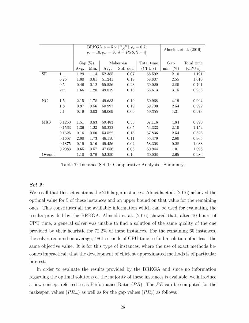
were computed using expression (1) defined in the previous section. Table 7 summarizes

these results in an aggregated form.

Table 6 has a total of 10 columns: (i) columns 1-3 indicate the instances’ characteristics;

(ii) columns 4-8 contain the results obtained with the BRKGA, and (iii) columns 9-10 refer

to the results provided by the heuristic of Almeida et al. (2016). More precisely, columns

4-5 are associated with the average and minimum gaps achieved, columns 6-7 depict the

average makespan values and their associated standard deviation, respectively and column

8 contains the total time associated with the 5 runs performed by the BRKGA. Columns

9-10 present the minimum gaps obtained by the heuristic proposed in Almeida et al. (2016)

and the associated total time, respectively. Table 7 follows the same structure of Table 6,

presented above.

From Table 6 we observe that the average and minimum gaps achieved by the BRKGA

improve the results provided by Almeida et al. (2016) in 26 and 27 out of the 36 classes

24

of instances, respectively. In terms of average and minimum gaps, the BRKGA achieved

the same results as the heuristic of Almeida et al. (2016) in 8 classes of instances, 7 of

which correspond to a gap of 0%. The BRKGA achieved 0% gaps for all instances in

10 and 19 classes of instances regarding average and minimum gaps, respectively. The

12 classes of instances whose minimum gaps obtained by the BRKGA are highlighted

in boldface indicate that the BRKGA was able to find the optimal value of all these 72

instances but the constructive heuristic of Almeida et al. (2016) was not. The higher gaps

achieved by the BRKGA are associated with instances having SF = variable, NC = 1.5,

MRS = 0.1667. The higher values of the standard deviation of the makespan occur more

commonly in the sets of instances associated with the smallest values of MRS. These

correspond to the hardest instances with fewer resources, hence having larger populations

and thus consuming more computational time. The last line of this table contains the

average results for the 216 instances and allow us to observe that the gaps were reduced

from 2.65% to 1.10% in the case of the average gaps and to 0.79% for the minimum gaps.

Hence, regarding the minimum gaps, the values provided by the BRKGA are roughly 3.4

times smaller than the ones achieved by Almeida et al. (2016). In terms of computational

time, the BRKGA requires an average time of one minute while the heuristic by Almeida

et al. (2016) needs on average one second. In spite of this difference in the computational

times, the supremacy of the BRKGA is clear in terms of the quality of the obtained gaps

and one minute of average time is not significant due to the complexity of the PSPFR.

25

BRKGA p = 5× dn×nK e, ρe = 0.7,

pe = 10, pm = 30, δ = PSS,G = n2

Almeida et al. (2016)

Gap (%) Makespan Total time

(CPU s)

Gap

min. (%)

Total time

(CPU s)SF NC MRS Avg. Min. Avg. Std. dev.

1 1.5 0.1250 6.33 6.13 52.433 0.15 61.027 9.47 1.096

0.1563 2.89 2.89 49.167 0.00 55.743 4.37 1.145

0.1875 0.00 0.00 48.667 0.00 56.852 0.00 1.374

1.8 0.1250 0.73 0.00 53.033 0.29 59.165 1.57 1.051

0.1563 1.19 0.79 47.667 0.15 54.801 1.92 1.195

0.1875 0.46 0.46 45.833 0.00 54.293 0.46 1.333

2.1 0.1250 0.00 0.00 64.167 0.00 60.835 1.07 1.103

0.1563 0.00 0.00 53.833 0.00 52.455 0.00 1.116

0.1875 0.00 0.00 56.667 0.00 54.155 0.00 1.304

0.75 1.5 0.1250 0.70 0.53 59.767 0.17 69.142 3.98 0.976

0.1667 0.33 0.00 44.133 0.17 57.961 0.90 1.000

0.2083 2.68 2.39 51.433 0.09 54.167 3.84 1.145

1.8 0.1250 2.04 0.82 60.433 0.61 66.369 6.47 0.916

0.1667 2.34 1.72 47.800 0.22 54.704 2.93 0.952

0.2083 0.00 0.00 49.833 0.00 52.925 0.00 1.117

2.1 0.1250 0.95 0.00 59.600 0.43 65.550 3.99 0.867

0.1667 0.00 0.00 43.167 0.00 56.201 0.00 0.984

0.2083 0.00 0.00 45.000 0.00 52.240 0.79 1.137

0.5 1.5 0.1250 1.79 0.26 61.633 0.83 81.355 6.17 0.749

0.1625 0.20 0.00 49.933 0.22 67.694 4.27 0.796

0.1875 0.51 0.51 41.667 0.00 64.173 0.88 0.890

1.8 0.1250 0.79 0.34 60.267 0.24 72.780 5.19 0.658

0.1625 0.29 0.00 55.467 0.24 70.753 2.42 0.872

0.1875 0.14 0.00 47.900 0.09 62.440 0.36 0.846

2.1 0.1250 0.42 0.00 71.967 0.45 78.988 5.00 0.713

0.1625 0.00 0.00 55.167 0.00 65.061 0.93 0.809

0.1875 0.00 0.00 56.000 0.00 57.938 0.00 0.783

var. 1.5 0.1250 3.12 1.58 52.467 0.61 60.477 7.55 0.765

0.1667 6.75 6.56 47.233 0.09 53.469 7.41 0.939

0.2083 0.49 0.49 37.667 0.00 49.560 1.42 1.049

1.8 0.1250 0.91 0.00 54.333 0.35 63.006 5.16 0.872

0.1667 2.08 2.08 45.667 0.00 55.702 4.02 1.002

0.2083 0.71 0.51 43.733 0.09 49.464 0.00 1.093

2.1 0.1250 0.38 0.32 63.700 0.07 66.694 2.46 0.916

0.1667 0.52 0.00 48.900 0.17 54.834 0.33 0.911

0.2083 0.00 0.00 54.667 0.00 47.308 0.00 1.033

Overall 1.10 0.79 52.250 0.16 60.008 2.65 0.986

Table 6: Instance Set 1: Comparative Analysis - Detail.

26

From Table 7 one can observe that, for the BRKGA, as SF decreases the gaps also

decrease while the associated computational effort increases. This increase may be justified

with the fact that instances with a smaller SF have fewer resources and thus originate

larger populations. For instances having SF = 0.5, the BRKGA achieved solutions which

correspond to an improvement of 6 and 22.8 times the results of Almeida et al. (2016),

regarding average and minimum gaps, respectively. Despite the instances associated with

SF = 1 being associated with a smaller improvement, the minimum gaps provided by the

BRKGA are roughly half of the ones obtained by Almeida et al. (2016).

In terms of the network complexity NC, an increase in this parameter leads, as ex-

pected, to a reduction in the gaps for the BRKGA. The BRKGA was able to reduce the

minimum gaps of the instances having NC = 2.1 to nearly 0%.

The instances with MRS = 0.1625 were the ones where the BRKGA produced the

smallest gaps with values of 0.16% and 0% for average and minimum gaps, respectively.

We point out that all these instances have SF = 0.5 and thus correspond to instances that

were among the hardest to tackle by Almeida et al. (2016). In this set of hard instances

we find also the ones associated with small values of MRS, such as MRS = 0.1250, were

the BRKGA originates minimum gaps of 0.83%. This correspond to a major improvement

since the heuristic of Almeida et al. (2016) produced gaps roughly 6 times higher.

27

BRKGA p = 5× dn×nK e, ρe = 0.7,

pe = 10, pm = 30, δ = PSS,G = n2

Almeida et al. (2016)

Gap (%) Makespan Total time

(CPU s)

Gap

min. (%)

Total time

(CPU s)Avg. Min. Avg. Std. dev.

SF 1 1.29 1.14 52.385 0.07 56.592 2.10 1.191

0.75 1.00 0.61 51.241 0.19 58.807 2.55 1.010

0.5 0.46 0.12 55.556 0.23 69.020 2.80 0.791

var. 1.66 1.28 49.819 0.15 55.613 3.15 0.953

NC 1.5 2.15 1.78 49.683 0.19 60.968 4.19 0.994

1.8 0.97 0.56 50.997 0.19 59.700 2.54 0.992

2.1 0.19 0.03 56.069 0.09 59.355 1.21 0.973

MRS 0.1250 1.51 0.83 59.483 0.35 67.116 4.84 0.890

0.1563 1.36 1.23 50.222 0.05 54.333 2.10 1.152

0.1625 0.16 0.00 53.522 0.15 67.836 2.54 0.826

0.1667 2.00 1.73 46.150 0.11 55.479 2.60 0.965

0.1875 0.19 0.16 49.456 0.02 58.308 0.28 1.088

0.2083 0.65 0.57 47.056 0.03 50.944 1.01 1.096

Overall 1.10 0.79 52.250 0.16 60.008 2.65 0.986

Table 7: Instance Set 1: Comparative Analysis - Summary.

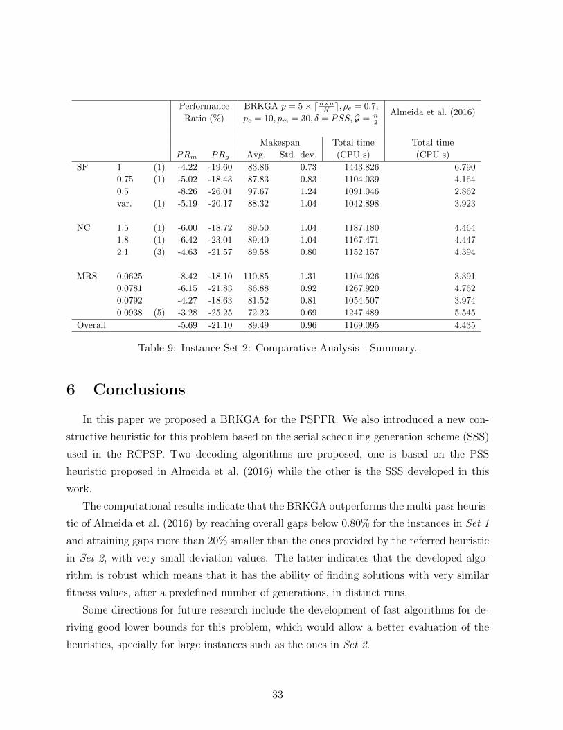
Set 2 :

We recall that this set contains the 216 larger instances. Almeida et al. (2016) achieved the

optimal value for 5 of these instances and an upper bound on that value for the remaining

ones. This constitutes all the available information which can be used for evaluating the

results provided by the BRKGA. Almeida et al. (2016) showed that, after 10 hours of

CPU time, a general solver was unable to find a solution of the same quality of the one

provided by their heuristic for 72.2% of these instances. For the remaining 60 instances,

the solver required on average, 4861 seconds of CPU time to find a solution of at least the

same objective value. It is for this type of instances, where the use of exact methods be-

comes impractical, that the development of efficient approximated methods is of particular

interest.

In order to evaluate the results provided by the BRKGA and since no information

regarding the optimal solutions of the majority of these instances is available, we introduce

a new concept referred to as Performance Ratio (PR). The PR can be computed for the

makespan values (PRm) as well as for the gap values (PRg) as follows:

28

PRm = ZB∗−ZH

ZH × 100%, regarding makespan values

PRg = DB∗−DH

DH × 100%, regarding gap values

where ZB∗

(DB∗) denotes the best upper bound (minimum gap) provided by the BRKGA

and ZH (DH) denotes the best upper bound (minimum gap) obtained by the heuristic

of Almeida et al. (2016). The gaps were computed using expression (1), presented in

Section 5.2, with the lower bound for each instance being equal to the length of the cor-

responding critical path. For example, if for one instance DB∗=8% and DH =10% then

PRg= -20% meaning that the BRKGA provide a gap 20% lower than the heuristic by

Almeida et al. (2016). The analysis of improvements also from the makespan point of

view (PRm) is of great interest when no lower bound besides the critical path length is

available. The latter is often a poor lower bound for this problem (Correia et al. 2012)

because it only considers information related to the precedence network. For fixed values

of SF and NC, a decrease of the value of MRS usually compromises the objective value,

contributing to its increase. The latter results in a larger distance between the optimal

value and the critical path length value. It is for this type of instances, particularly when

the best known lower bound is eventually poor, that the use of a makespan performance

measure is of great importance.

Table 8 presents the detailed results for each class of instances defined by the combina-

tion of the values of SF , NC and MRS. Each row of this Table corresponds to an average

of 6 instances. These results are summarized in Table 9.

The 10 columns of Table 8 have the following meaning: (i) columns 1-4 contain the char-

acteristics of each class of instances; (ii) columns 5 and 6 show the results associated with

the PR values in terms of makespan (PRm) and gap (PRg), respectively; (iii) columns 7-9

present the results obtained by the proposed BRKGA, namely average makespan, standard

deviation and total CPU time taken in the 5 runs, respectively; and (iii) column 10 depicts

the total time required by the heuristic proposed by Almeida et al. (2016). The BRKGA

also found the optimal solutions for all the 5 instances for which Almeida et al. (2016)

identified their optimal value. We did not take into account these instances for computing

the values presented in this table and therefore we indicate, in the untitled column 4, inside

parentheses, the number of instances not considered for the results presented. Table 9 is

structured as Table 8.

29

From Table 8 we observe a general improvement in terms of both PRm and PRg. The

BRKGA performed better than the heuristic of Almeida et al. (2016) in all the 36 classes

of instances. The best results in terms of PRm were generally attained for the instances

associated with smaller values of MRS, with a particular emphasis for the instances having

SF = 0.5 and MRS = 0.0625. In fact, the class of instances which reported the highest

improvement regarding PRm (13%) is actually defined by SF = 0.5, NC = 1.5 and

MRS = 0.0625. It was also the one associated with the highest standard deviation of the

average makespan value, which indicates an increased difficulty faced by the BRKGA in

attaining solutions of the same fitness consistently for these instances. Analyzing the PRg

values, these seem to follow a different direction. This can be associated with the fact

of smaller makespan values being associated with instances having higher values of MRS

which may allow a greater degree of parallelization, for fixed SF and NC values. In fact,

considering SF = 0.5, the class of instances with NC = 2.1 and MRS = 0.0938 is the one

associated with the smallest improvement in the makespan (PRm = −2.30%) and the one

having the greatest gap improvement (PRg = −35.18%), hence validating our reasoning

of evaluating the results of the BRKGA in terms of gap and makespan improvement from

the results of Almeida et al. (2016).

30

Performance

Ratio (%)

BRKGA p = 5× dn×nK e, ρe = 0.7,

pe = 10, pm = 30, δ = PSS,G = n2

Almeida et al. (2016)

Makespan Total time

(CPU s)

Total time

(CPU s)SF NC MRS PRm PRg Avg. Std. dev.

1 1.5 0.0625 -5.92 -11.79 97.90 0.78 1158.783 4.718

0.0781 -4.36 -12.77 79.30 0.85 1478.504 6.726

0.0938 (1) -3.06 -18.70 70.48 0.69 1791.673 9.007

1.8 0.0625 -6.49 -14.61 100.53 1.03 1136.121 4.598

0.0781 -5.17 -27.61 82.40 0.83 1455.465 6.634

0.0938 (1) -2.41 -33.12 65.16 0.60 1776.367 9.009

2.1 0.0625 -5.33 -14.10 100.00 0.77 1132.525 4.611

0.0781 -3.02 -19.39 85.90 0.56 1451.702 6.632

0.0938 -1.68 -26.39 67.73 0.46 1726.694 9.176

0.75 1.5 0.0625 -6.20 -12.67 110.30 0.66 1119.035 3.356

0.0792 -4.75 -14.07 81.97 0.86 1102.655 4.085

0.0938 -3.64 -16.33 69.80 0.61 1135.340 5.213

1.8 0.0625 -8.54 -16.92 110.73 1.07 1142.319 3.335

0.0792 -4.83 -19.95 83.77 0.96 1092.978 4.182

0.0938 (2) -3.52 -27.59 70.80 0.87 1115.094 5.101

2.1 0.0625 -7.73 -20.69 108.97 1.11 1076.178 3.257

0.0792 -3.32 -19.42 77.40 0.67 1045.309 4.005

0.0938 -1.44 -18.13 71.15 0.54 1109.151 4.940

0.5 1.5 0.0625 -13.86 -25.82 120.77 2.41 1139.316 2.468

0.0781 -9.22 -20.41 98.43 1.39 1127.840 2.965

0.0938 -3.62 -24.49 81.50 0.83 1100.186 3.231

1.8 0.0625 -12.77 -25.88 129.20 1.71 1087.627 2.398

0.0781 -8.58 -27.97 88.17 1.19 1050.740 2.820

0.0938 -6.85 -29.21 77.57 0.94 1134.217 3.489

2.1 0.0625 -10.60 -22.31 120.93 1.63 1109.013 2.510

0.0781 -6.58 -22.85 87.10 0.72 1043.272 2.796

0.0938 -2.30 -35.18 75.40 0.32 1027.204 3.085

var 1.5 0.0625 -7.68 -13.21 110.37 1.57 1116.957 3.286

0.0792 -6.23 -24.12 79.53 1.08 1015.154 3.778

0.0938 -2.99 -30.28 70.47 0.74 1061.472 4.731

1.8 0.0625 -9.57 -21.46 111.07 1.70 1033.412 3.075

0.0792 -3.40 -14.15 77.97 0.72 1017.991 3.820

0.0938 -4.24 -19.31 71.40 0.79 1068.803 4.906

2.1 0.0625 -6.37 -17.71 109.43 1.29 997.032 3.080

0.0792 -3.08 -20.06 88.47 0.54 1052.956 3.973

0.0938 (1) -2.74 -21.49 73.72 0.89 1018.186 4.658

Overall (5) -5.69 -21.10 89.49 0.96 1169.095 4.435

Table 8: Instance Set 2: Comparative Analysis - Detail.

31

From Table 9 we observe a global improvement from the solutions provided by the

heuristic. The quality of the results achieved by the BRKGA increases as the values of

SF become smaller. Smaller values of SF lead to smaller computational effort. Due to

their hardness, instances having SF = 0.5 are associated with higher values of standard

deviation of makespan, approximately 1.27% of their average makespan value, a similar

behavior to what was observed for Set 1. Moreover these instances achieved the best

results regarding both PRm and PRg. Overall, and as expected, an increase in the NC

leads to a slight decrease in computational time. We note that the 3 (out of the 5)

instances where the heuristic of Almeida et al. (2016) reached the optimal solution, are

associated with NC = 2.1. Instances having higher values of NC usually tend to be

easier because potentially a smaller number of activities can be processed in parallel due

to the increased number of precedence relations, for a fixed number of activities. Amongst

the different NC values, the largest improvements in terms of both PRm and PRg were

achieved for the instances having NC = 1.8. Regarding MRS, the best results in terms

of PRm and PRg are associated with MRS = 0.0625 and MRS = 0.0938, respectively.

The latter is explained by the fact of the instances associated with higher values of MRS

values being associated with smaller values of average makespan, and as discussed before,

these instances tend to allow a greater degree of parallelization which tend to allow their

corresponding optimal values to be closer to the value of the associated critical path length.

We noticed that the 5 instances for which the heuristic of Almeida et al. (2016) attains

their optimal solutions, belong to the set of instances having the most resources, associated

with the highest value of MRS considered: MRS = 0.0938. We observe overall values

of PRm = −5.69% and PRg = −21.10%. This constitutes a great improvement from the

results attained by the previously developed multi-pass heuristic in Almeida et al. (2016).

The standard deviation values are larger for instances having smaller values of SF , NC

or MRS. In terms of computational time, we must not forget that these instances have

roughly the double of resources and activities as well as a population and a stopping

criterion with twice the size of the ones considered in Set 1.

32

Performance

Ratio (%)

BRKGA p = 5× dn×nK e, ρe = 0.7,

pe = 10, pm = 30, δ = PSS,G = n2

Almeida et al. (2016)

Makespan Total time

(CPU s)

Total time

(CPU s)PRm PRg Avg. Std. dev.

SF 1 (1) -4.22 -19.60 83.86 0.73 1443.826 6.790

0.75 (1) -5.02 -18.43 87.83 0.83 1104.039 4.164

0.5 -8.26 -26.01 97.67 1.24 1091.046 2.862

var. (1) -5.19 -20.17 88.32 1.04 1042.898 3.923

NC 1.5 (1) -6.00 -18.72 89.50 1.04 1187.180 4.464

1.8 (1) -6.42 -23.01 89.40 1.04 1167.471 4.447

2.1 (3) -4.63 -21.57 89.58 0.80 1152.157 4.394

MRS 0.0625 -8.42 -18.10 110.85 1.31 1104.026 3.391

0.0781 -6.15 -21.83 86.88 0.92 1267.920 4.762

0.0792 -4.27 -18.63 81.52 0.81 1054.507 3.974

0.0938 (5) -3.28 -25.25 72.23 0.69 1247.489 5.545

Overall -5.69 -21.10 89.49 0.96 1169.095 4.435

Table 9: Instance Set 2: Comparative Analysis - Summary.

6 Conclusions

In this paper we proposed a BRKGA for the PSPFR. We also introduced a new con-

structive heuristic for this problem based on the serial scheduling generation scheme (SSS)

used in the RCPSP. Two decoding algorithms are proposed, one is based on the PSS

heuristic proposed in Almeida et al. (2016) while the other is the SSS developed in this

work.

The computational results indicate that the BRKGA outperforms the multi-pass heuris-

tic of Almeida et al. (2016) by reaching overall gaps below 0.80% for the instances in Set 1

and attaining gaps more than 20% smaller than the ones provided by the referred heuristic

in Set 2, with very small deviation values. The latter indicates that the developed algo-

rithm is robust which means that it has the ability of finding solutions with very similar

fitness values, after a predefined number of generations, in distinct runs.

Some directions for future research include the development of fast algorithms for de-

riving good lower bounds for this problem, which would allow a better evaluation of the

heuristics, specially for large instances such as the ones in Set 2.

33

Acknowledgements

This work was supported by National Funding from FCT - Fundacao para a Ciencia e a

Tecnologia, under the projects Fundacao para a Ciencia e a Tecnologia, UID/MAT/04561/2013

(CMAF-CIO/FCUL) and UID/MAT/00297/2013 (CMA/FCT/UNL).

References

Almeida, B. F., Correia, I., and Saldanha-da-Gama, F. (2015). An Instance Generator

for the Multi-Skill Resource-Constrained Project Scheduling Problem. Technical report,

Faculdade de Ciencias da Universidade de Lisboa — Centro de Matematica, Aplicacoes

Fundamentais e Investigacao Operacional. Available at https://ciencias.ulisboa.

pt/sites/default/files/fcul/unidinvestig/cmaf-cio/SGama.pdf.

Almeida, B. F., Correia, I., and Saldanha-da-Gama, F. (2016). Priority-based heuristics

for the multi-skill resource constrained project scheduling problem. Expert Systems with

Applications, 57:91–103.

Bean, J. C. (1994). Genetic algorithms and random keys for sequencing and optimization.

ORSA Journal on Computing, 6(2):154–160.

Brucker, P., Drexl, A., Mohring, R., Neumann, K., and Pesch, E. (1999). Resource-

constrained project scheduling: Notation, classification, models, and methods. European

Journal of Operational Research, 112(1):3–41.

Correia, I., Lourenco, L. L., and Saldanha-da-Gama, F. (2012). Project scheduling with

flexible resources: formulation and inequalities. OR Spectrum, 34:635–663.

Correia, I. and Saldanha-da-Gama, F. (2014). The impact of fixed and variable costs in

a multi-skill project scheduling problem: An empirical study. Computers & Industrial

Engineering, 72:230–238.

Correia, I. and Saldanha-da-Gama, F. (2015). A modeling framework for project staffing

and scheduling problems. In Schwindt, C. and Zimmermann, J., editors, Handbook on

Project Management and Scheduling, volume 1, pages 547–564. Springer.

34

Demeulemeester, E. L. and Herroelen, W. (2002). Project Scheduling: A Research Hand-

book. Springer.

Goldberg, D. E. (1989). Genetic Algorithms in Search, Optimization and Machine Learn-

ing. Addison-Wesley Longman Publishing Co., Inc.

Goncalves, J., Mendes, J., and Resende, M. (2008). A genetic algorithm for the resource

constrained multi-project scheduling problem. European Journal of Operational Re-

search, 189(3):1171 – 1190.

Goncalves, J. F. and Resende, M. G. (2011). Biased random-key genetic algorithms for

combinatorial optimization. Journal of Heuristics, 17:487–525.

Goncalves, J. F. and Resende, M. G. (2013). A biased random key genetic algorithm

for 2D and 3D bin packing problems. International Journal of Production Economics,

145(2):500 – 510.

Goncalves, J. F. and Resende, M. G. (2015). A biased random-key genetic algorithm for

the unequal area facility layout problem. European Journal of Operational Research,

246(1):86 – 107.

Goncalves, J. F., Resende, M. G., and Mendes, J. J. (2011). A biased random-key ge-

netic algorithm with forward-backward improvement for the resource constrained project

scheduling problem. Journal of Heuristics, 17(5):467–486.

Gutjahr, W. J., Katzensteiner, S., Reiter, P., Stummer, C., and Denk, M. (2008).

Competence-driven project portfolio selection, scheduling and staff assignment. Cen-

tral European Journal of Operations Research, 16:281–306.

Hartmann, S. (2002). A self-adapting genetic algorithm for project scheduling under re-

source constraints. Naval Research Logistics (NRL), 49(5):433–448.

Hartmann, S. and Briskorn, D. (2010). A survey of variants and extensions of the resource-

constrained project scheduling problem. European Journal of Operational Research,

207(1):1–14.

Heimerl, C. and Kolisch, R. (2010). Scheduling and staffing multiple projects with a multi-

skilled workforce. OR Spectrum, 32:343–368.

35

Herroelen, W. S. and Demeulemeester, E. L. (1998). Resource-constrained project schedul-

ing: A survey of recent developments. Computers and Operations Research, 25:279–302.

Holland, J. H. (1975). Adaptation in Natural and Artificial Systems. University of Michigan

Press.

Klein, R. (2000). Bidirectional planning: improving priority rule-based heuristics for

scheduling resource-constrained projects. European Journal of Operational Research,

127:619–638.

Kolisch, R. (1996). Serial and parallel resource-constrained project scheduling methods re-

visited: Theory and computation. European Journal of Operational Research, 90(2):320

– 333.

Li, H. and Womer, K. (2009). Scheduling projects with multi-skilled personnel by a hybrid

MILP/CP benders decomposition algorithm. Journal of Scheduling, 12:281–298.

Li, K. and Willis, R. (1992). An alternative scheduling technique for resource constrained

project scheduling. European Journal of Operational Research, 56:370–379.

Mendes, J., Goncalves, J., and Resende, M. (2009). A random key based genetic algorithm

for the resource constrained project scheduling problem. Computers and Operations

Research, 36(1):92 – 109.

Ozdamar, L. (1999). A genetic algorithm approach to a general category project scheduling

problem. IEEE Transactions on Systems, Man and Cybernetics, 29:44–69.

Ruiz, E., Albareda-Sambola, M., Fernandez, E., and Resende, M. G. (2015). A biased

random-key genetic algorithm for the capacitated minimum spanning tree problem. Com-

puters and Operations Research, 57(C):95–108.

Spears, W. M. and Jong, K. A. D. (1991). On the virtues of Parameterized Uniform

Crossover. In Proceedings of the Fourth International Conference on Genetic Algorithms,

pages 230–236.

Weglarz, J., Jozefowska, J., Mika, M., and Waligora, G. (2011). Project scheduling with

finite or infinite number of activity processing modes - a survey. European Journal of

Operational Research, 208:177–205.

36