1

A Behavioral Study of Capacity Allocation in Revenue Management

Bahriye Cesaret • Elena Katok

Faculty of Business, Özuegin Üniveritesi, Istanbul, Turkey 34794 The Jindal School of Management, University of Texas at Dallas, Richardson, TX 75080

bahriye.cesaret@ozyegin.edu.tr • ekatok@utdallas.edu

Abstract

In this paper, we present a set of laboratory experiments that investigate how human subjects solve the two-class capacity allocation revenue management problem. The two-class problem is a basic revenue management problem and it is a fundamental building block for more sophisticated problems. We study the capacity allocation problem with ordered and unordered arrivals, as well as a simplified version of the problem in which the decision-maker makes a single capacity allocation decision up-front. We find that our laboratory participants generally accept too many low-type customers, leave too few units of unused capacity, and as a result serve too few high-type customers. We also find that making decisions up-front improves performance in the ordered arrivals case, and does not hurt performance in the unordered arrivals case. Lastly, we propose a behavioral choice model which incorporates the participants’ regret feelings and organizes our experimental data well. Key words: Behavioral Operations, Revenue Management, Capacity Allocation, Sequential Decision Making, Regret.

1. Introduction

The practice of Revenue Management (RM) is considered to be one of the biggest success stories of

Operations Research. Originated by Sabre (www.sabre.com) in 1970s, it is credited for increasing the

revenue gains of the airline industry by 5-7% (Donovan 2005), and has since been adopted by industries

that share some of the airline industry’s characteristics (hotel, car rental, media and broadcasting, cruise

lines and ferry lines, theaters and sporting events and so on). The essence of RM is price discrimination—

charging different prices to different customers for what is essentially the same product. Product attributes

that make RM effective include fixed and highly perishable capacity that requires to be sold in advance of

consumption, highly variable demand, and a heterogeneous customer base (Talluri 2012).

In many industries, RM models and software automatically control the bulk of inventory (Talluri

and Van Ryzin (2004) describe implementation details for such traditional RM industries as airlines and

2

hotels), but even these traditional users of RM must combine RM software with manual oversight to achieve

the best results (Talluri 2012). This managerial augmentation of automated system is useful due to the

inevitable presence of exceptions (special days or events). So RM software does not fully replace human

judgment even in traditional industries in which the majority of the decisions are automated. There are also

many industries with some characteristics that make them candidates for benefitting from some of the RM

methods and techniques, which usually do not widely use RM software. Examples include restaurants, spa

resorts, golf courses (Kimes 2003) and many other small businesses that still involve managers in RM

decisions. Some of the RM decisions made by these smaller businesses range from accepting appointments

for a hair-saloon, to deciding how much beer to deliver at each store along a delivery route (Bassok and

Ernst 1995), to how many bagels to reserve for sandwiches at lunch (Gerchak et al. 1985).

At the heart of all these RM problems lies the basic tradeoff—to sell a product at a lower price, or

to forego this certain revenue by postponing the sale in hopes of higher revenue in the future, while also

accepting a risk of leaving the unit unsold. Our goal in this research is to understand how human decision

makers solve a basic RM problem (the single-resource independent class problem) that is a fundamental

building block for more sophisticated RM problems. A good understanding of how human decision makers

solve this problem is an important step towards being able to predict and evaluate more complex settings.

Specifically, in this paper we attempt to answer the following three questions:

(i) Do human decision makers allocate their capacity optimally?

(ii) If the answer to the first question is in the negative, then what kind of behavioral regularities do

they exhibit while making RM decisions?

(iii) What behavioral decision rules, if any, govern their capacity allocation decisions?

Literature describing the theory and practice of RM is quite vast, and we do not attempt to provide

a comprehensive review here. We refer the reader to Özer and Phillips (2012) for a comprehensive review

of pricing management. The work on ordered arrivals (static) capacity allocation decisions can be found in

3

Littlewood (1972), Belobaba (1989), Curry (1990), Wollmer (1992), Brumelle and McGill (1993),

Robinson (1995); and unordered arrivals (dynamic) models are covered in Lee and Hersh (1993) and

Lautenbacher and Stidham (1999). Talluri and Van Ryzin (2004) describe more recent developments in

RM.

Our study falls into the area of behavioral operations management, since we use controlled

laboratory experiments with human participants to test analytical models (see Katok (2011) for an overview

of this literature). There are fewer behavioral than analytical studies of problems related to RM and

dynamic pricing. Bearden et al. (2008) consider a firm selling a fixed number of units and facing uncertain

demand for the product. In their setting, each customer has a different willingness-to-pay for the product

and makes a price offer to purchase a unit of the product. Firm needs to decide whether to accept or reject

an arriving offer. The authors try to understand what kind of decision policies (sophisticated policies vs.

simple heuristics) the decision makers employ while making RM decision. Our problem studied in

unordered arrivals setting is similar to Bearden et al. (2008)’s setup, however it also differs from it in several

aspects. Their problem considers multiple (to be precise infinite) customer segments and mainly aims to

investigate the behavior in pricing RM decisions, while we focus on a problem with fixed prices and two

customer segments and aim to investigate the behavior in capacity allocation RM decisions. In addition,

they study the problem in unordered arrivals setting, whereas we consider our problem in both ordered and

unordered arrivals settings. Our aim with this design is to build a bridge between simple (ordered arrivals)

and sophisticated (unordered arrivals) RM models, which can enable us to understand the human behavior

thoroughly, starting from a simple model and building on it gradually.

Bendoly (2011) examines the physiological responses of decision makers engaged in RM tasks.

Bendoly (2011) uses the Bearden et al. (2008)’s design and varies the number of tasks that are

simultaneously presented to decision makers. The author argues that disparity between actual and

normative behavior are due to arousal and stress associated with RM tasks.

4

Kocabıyıkoğlu et al. (2015) study the two-class RM problem and a closely related newsvendor

problem, and test whether the behavior in these two mathematically equivalent models are the same in the

laboratory. They find that participants’ RM decisions (protection levels) are consistently higher compared

to the newsvendor order quantities. The authors argue that minimizing unsold units becomes more salient

in the newsvendor problem, and this may explain why participants order fewer units in the newsvendor

problem than the RM problem.

Apart from the analysis of seller’s behavior in RM problems, there are several behavioral studies

investigating buyers’ behavior in this context, specifically studying strategic customer behavior; see, e.g.,

Kremer et al. (2013), Osadchiy and Bendoly (2011), Mak et al. (2012), Li et al. (2011), Hendel and Nevo

(2006), Nair (2007).

Finally, we consider the effect of regret on capacity allocation decisions, therefore another research

stream that is related to ours is the literature studying the effect of regret on individuals’ decisions. There

exists a good body of literature which demonstrates the effect of regret in decision making. We refer the

reader to Zeelenberg et al. (2000) for a review on this topic. There are few studies in operations

management that consider the role of regret. Examples include Engelbrecht-Wiggans and Katok (2007)

(auctions), Perakis and Roels (2008) (newsvendor problem), Diecidue et al. (2012) (dynamic purchase),

Nasiry and Popescu (2012) (advance selling), Özer and Zheng (2016) (markdown management). We add

to this literature by studying regret in a new context; i.e., revenue management.

We already pointed out that the analytic side of optimally allocating the capacity of a limited,

perishable resource to different customer segments with the goal of revenue maximization is a well-studied

problem in the operations management literature. We contribute to the RM literature by studying how

human decision makers solve this problem, and proposing a behavioral choice model which uses the

intuition that comes from an extension of the theoretical model and can account for a portion of the

deviations observed from the optimal decision policy.

5

The remainder of the paper is organized as follows. In Section 2, we explain the models and settings

in this study. We discuss the details of our experimental design and laboratory implementations in Section

3. We provide theoretical benchmarks and formulate our hypotheses in Section 4. Section 5 presents the

experimental results. In Section 6, we present an extension to the theoretical model and propose a

behavioral choice model that utilizes the intuition coming from the extended model. Section 7 concludes

the paper.

2. The Models and Settings

We consider the single-resource RM problem with two independent customer classes (the low-type has a

low willingness-to-pay, and the high-type has a high willingness-to-pay). Our human participants (who are

in the role of the manager of a firm) must decide whether to accept or reject an arriving customer to

maximize their revenues. Prices are exogenous. We chose this setting because it is the simplest instance

of RM problems and is a basic building block for a general class of models.

The two main treatments in this study are the ordered arrivals and the unordered arrivals

treatments. In both treatments, for each customer that arrives, the participants, knowing the customer type

(high-type who pay 𝑝" or low-type who pay 𝑝#), decide whether to accept this customer or to turn it away.

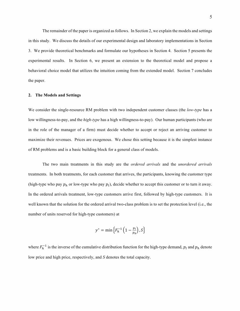
In the ordered arrivals treatment, low-type customers arrive first, followed by high-type customers. It is

well known that the solution for the ordered arrival two-class problem is to set the protection level (i.e., the

number of units reserved for high-type customers) at

𝑦∗ = min 𝐹"+, 1 − /0/1

, 𝑆

where 𝐹"+, is the inverse of the cumulative distribution function for the high-type demand, 𝑝# and 𝑝" denote

low price and high price, respectively, and S denotes the total capacity.

6

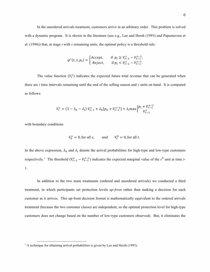
In the unordered arrivals treatment, customers arrive in an arbitrary order. This problem is solved

with a dynamic program. It is shown in the literature (see e.g., Lee and Hersh (1993) and Papastavrou et

al. (1996)) that, at stage t with s remaining units, the optimal policy is a threshold rule:

𝜑∗ 𝑡, 𝑠, 𝑝# =𝐴𝑐𝑐𝑒𝑝𝑡, if𝑝# ≥ 𝑉>+,? − 𝑉>+,?+,;𝑅𝑒𝑗𝑒𝑐𝑡, if𝑝# < 𝑉>+,? − 𝑉>+,?+,.

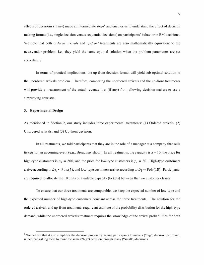
The value function (𝑉>?) indicates the expected future total revenue that can be generated when

there are t time intervals remaining until the end of the selling season and s units on hand. It is computed

as follows:

𝑉>? = 1 − 𝜆" − 𝜆# 𝑉>+,? + 𝜆" 𝑝" + 𝑉>+,?+, + 𝜆#max𝑝# + 𝑉>+,?+,

𝑉>+,?

with boundary conditions

𝑉J? = 0, forall𝑠, and𝑉>J = 0, forall𝑡.

In the above expression, 𝜆" and 𝜆# denote the arrival probabilities for high-type and low-type customers

respectively.1 The threshold (𝑉>+,? − 𝑉>+,?+,) indicates the expected marginal value of the sth unit at time t-

1.

In addition to the two main treatments (ordered and unordered arrivals) we conducted a third

treatment, in which participants set protection levels up-front rather than making a decision for each

customer as it arrives. This up-front decision format is mathematically equivalent to the ordered arrivals

treatment (because the two customer classes are independent, so the optimal protection level for high-type

customers does not change based on the number of low-type customers observed). But, it eliminates the

1 A technique for obtaining arrival probabilities is given by Lee and Hersh (1993).

7

effects of decisions (if any) made at intermediate steps2 and enables us to understand the effect of decision

making format (i.e., single decision versus sequential decisions) on participants’ behavior in RM decisions.

We note that both ordered arrivals and up-front treatments are also mathematically equivalent to the

newsvendor problem, i.e., they yield the same optimal solution when the problem parameters are set

accordingly.

In terms of practical implications, the up-front decision format will yield sub-optimal solution to

the unordered arrivals problem. Therefore, comparing the unordered arrivals and the up-front treatments

will provide a measurement of the actual revenue loss (if any) from allowing decision-makers to use a

simplifying heuristic.

3. Experimental Design

As mentioned in Section 2, our study includes three experimental treatments: (1) Ordered arrivals, (2)

Unordered arrivals, and (3) Up-front decision.

In all treatments, we told participants that they are in the role of a manager at a company that sells

tickets for an upcoming event (e.g., Broadway show). In all treatments, the capacity is S = 10, the price for

high-type customers is 𝑝" = 200, and the price for low-type customers is 𝑝# = 20. High-type customers

arrive according to 𝐷ℎ ∼ Pois(5), and low-type customers arrive according to 𝐷𝑙 ∼ Pois(15). Participants

are required to allocate the 10 units of available capacity (tickets) between the two customer classes.

To ensure that our three treatments are comparable, we keep the expected number of low-type and

the expected number of high-type customers constant across the three treatments. The solution for the

ordered arrivals and up-front treatments require an estimate of the probability distribution for the high-type

demand, while the unordered arrivals treatment requires the knowledge of the arrival probabilities for both

2 We believe that it also simplifies the decision process by asking participants to make a (“big”) decision per round, rather than asking them to make the same (“big”) decision through many (“small”) decisions.

8

high-type (𝜆ℎ) and low-type (𝜆𝑙) customers in each interval 𝑡. 3 We also keep the underlying demand

distributions for each customer class the same across the three treatments. To achieve this, we choose

Poisson distribution to model the demand, and utilize ‘Poisson to binomial approximation’ to obtain arrival

probabilities for the unordered arrivals treatment. We chose these specific demand and capacity parameters

to ensure that RM decisions are relevant (i.e., capacity is binding).

At the beginning of each decision round participants see capacity, price and demand information.4

Also, in all treatments, participants know that there will be at least 10 low-type customers. Demand

information that participants observe and the feedback information they see at the end of each round, vary

across treatments.

In ordered and unordered arrival treatments, we tell the participants that each round of the game

consists of multiple periods. In each period, a customer arrives with a certain probability. In the ordered

arrivals treatment, we tell participants that low-type customers arrive first, and high-type customers arrive

after all low-type customers have arrived. In the unordered arrivals treatment, we tell participants that each

period a low-type customer arrives with probability 𝜆𝑙

= 0.0244, or a high-type customer arrives with

probability 𝜆ℎ

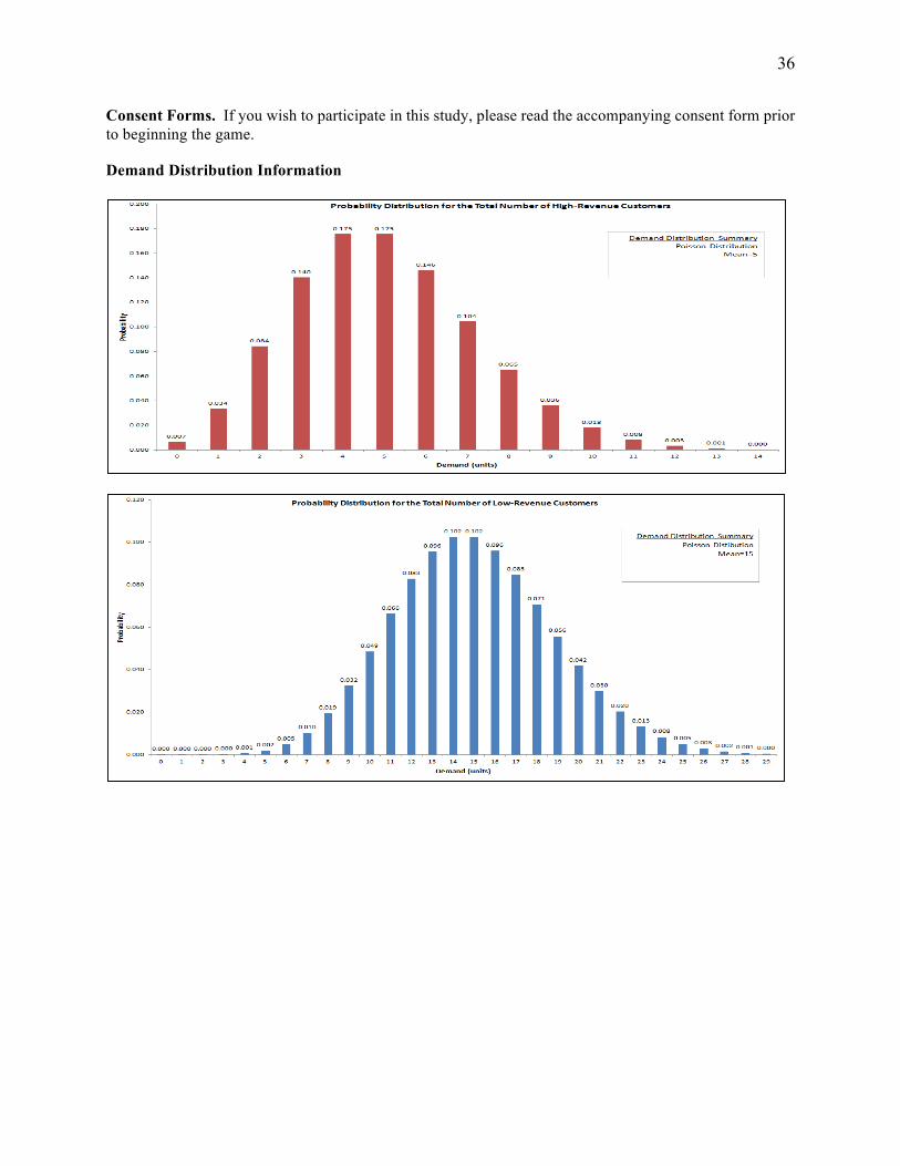
= 0.0083 (but never both). We also provide the participants with the probability

distributions (displayed graphically and described as “Poisson” with the mean) for the total number of both

high-type and low-type5 customers.

Each round consists of 600 time periods. Whenever a customer arrives, a participant observes the

type of the customer (high or low), remaining capacity in the current round, (remaining number of periods

in the current round in the unordered arrivals treatment), and capacity that has already been allocated to

high-type and to low-type customers, and her revenue earned so far in the current round. Then, the

3 We use fixed arrival probabilities for each t, thus instead of 𝜆"(t) (resp., 𝜆#(𝑡)), we use the notation 𝜆" (resp., 𝜆#). 4The vector of actual demand was determined prior to the experiment and was the same for every subject. 5 In ordered arrivals treatment, subjects observe low-class arrivals before they start to observe high-class arrivals, thus we also provide them low-class demand information, although it is not required by the optimal policy.

9

participant is asked to either accept or reject the new arrival. Once a round ends (which happens either

when all 10 units of capacity have been allocated or when the last customer has arrived), the participant

sees feedback information on how many units were allocated to each of the customer type, realized high-

type and low-type demands, the unused capacity, and the resulting total revenue for this round.

In the up-front treatment, we tell the participants the probability distribution for high-type demand,

again, described as “Poisson” with the specified mean, and displayed graphically. To avoid providing

participants with irrelevant information, we simply tell them that low-type demand will be at least 10 units

(and do not show them low-type demand distribution). At the beginning of each decision making round,

participants decide how many of the 10 units of capacity they want to reserve for high-type customers.

After the decision is made, participants see feedback information on the outcome of the round: the number

of units reserved for high-type customers, realized high-type demand, the resulting unused capacity, and

their resulting revenue for this round.

In total, 75 human subjects participated in our study: 24 in the ordered arrivals, 26 in the unordered

arrivals, and 25 in the up-front treatment. Each person participated in a single treatment only (this is a

between-subject design). In all treatments, upon arrival to the laboratory, the participants were randomly

seated in visually isolated cubicles and were provided written instructions that describe the rules of the

game, the use of the software, and the payment procedures (see Appendix A for the instructions used in the

unordered arrivals treatment; instructions for other treatments are similar and available upon request). After

all participants had a chance to read the instructions on their own, the experimenter read the instructions to

them aloud, invited participants to ask questions, and answered any questions before starting the session.

The same experimenter conducted all sessions in this study. Experiments consisted of 40 decision rounds

(with ordered and unordered arrival treatments having multiple decisions in each round), thus each subject

played the game 40 times. In all treatments, as the rounds progressed, subjects received historical

information about the outcomes in prior rounds of the game.

10

All treatments were conducted at a major U.S. public university. Participants were recruited

through the on-line recruitment system ORSEE (Greiner 2004). The experimental interface was

programmed using the zTree system (Fischbacher 2007) for all treatments. The snapshots of the computer

screens for the unordered arrivals treatment are provided in Appendix B.

Subjects made their decisions and received experimental currency units (ECUs) based on the

revenues they earned. Cash was the only incentive offered to the participants. The total ECUs across all

40 rounds were converted to cash payments at the end of the session at the rate of 3000 ECUs = $1 US.

The average earnings for all treatments were $18.01 US dollars, including a $5 US dollars participation fee

for each subject. Sessions lasted between 50 and 80 minutes.

4. Theoretical Benchmarks and Research Hypotheses

Table 1 summarizes theoretical benchmarks for the optimal solutions for the three treatments in our study.

Table 1. Theoretical Benchmarks.

Treatment High-type customers served

Low-type customers served

Unused capacity Average revenue

Ordered Arrivals 4.800 2.000 3.200 1000.00

Unordered Arrivals 4.850 4.075 1.075 1051.50

Up-front 4.800 2.000 3.200 1000.00

We formulate research hypotheses based on these theoretical benchmarks, because we first want to

understand how well the theory describes the actual capacity allocation decisions in RM.

Hypothesis 1: In all three treatments, the average performance will not be significantly different from the

optimal performance.

11

(A) The Strong Performance Hypothesis: The average number of high-type customers served, the average

number of low-type customers served, the unused capacity (and therefore the average revenue earned) will

not be significantly different from the corresponding theoretical benchmarks in Table 1.

(B) The Weak Performance Hypothesis: The average revenue earned will not be significantly different from

the corresponding theoretical benchmark in Table 1.

Hypothesis 1A allows us to see how participants allocate their capacity relative to the optimal

allocation, whereas Hypothesis 1B allows us to check whether participants can reach the normative revenue

level while allocating their capacity in a different way compared to the optimal policy.

Note that only decision-making format changes across ordered arrivals and up-front treatments.

Theory predicts that the performance across these two treatments will be the same and also equal to the

optimal performance. We formulate a weaker version of this prediction which states that the performance

across the two treatments will be the same, but not necessarily equal to the optimal performance.

Hypothesis 2: Assuming ordered arrivals, the performance in the ordered arrivals and the up-front

treatments will not be significantly different. Specifically, the average number of high-type customers

served, the average number of low-type customers served, the unused capacity, and therefore the average

revenue will be the same across the two treatments.

Finally, making an up-front decision yields suboptimal solution for the unordered arrivals

treatment; it’s not clear how the number of low and high-type customers served, and the unused capacity

will change, however we can expect that the average revenue earned may suffer in the earlier treatment,

which is stated as our third hypothesis.

Hypothesis 3: Assuming unordered arrivals, the average revenue earned in the up-front treatment will be

less than the average revenue earned in the unordered arrivals treatment.

12

5. Experimental Results

5.1 Do Participants Allocate Their Capacity Optimally?

Table 2 presents descriptive statistics for the number of both high-type and low-type customers served,

unused capacity, and the resulting revenues earned in the three treatments, including the mean, and the

standard errors (in parentheses). We use individual subject (taking averages over 40 rounds per subject) as

the unit of analysis and the Wilcoxon Signed-Rank Test to compare each entry in Table 2 with its

corresponding theoretical benchmark (Table 1). We indicate the entries that are significantly different from

their theoretical benchmark by an asterisk in Table 2.

Table 2. Descriptive Statistics

Treatment High-type customers served

Low-type customers served

Unused capacity Average revenue

Ordered Arrivals

4.194*

(0.069) 4.001* (0.243)

1.805* (0.184)

918.77* (9.593)

Unordered Arrivals

4.340* (0.066)

4.357 (0.183)

1.303 (0.143)

955.21* (10.862)

Up-front 4.525* (0.059)

2.970* (0.265)

2.505* (0.214)

964.40* (7.564)

Notes. *p < 0.001. The standard errors are in parentheses.

The results show that in all treatments almost every metric is significantly different from its theoretical

benchmark, contrary to Hypothesis 1A. Also contrary to Hypothesis 1B, in all treatments participants earn

significantly lower revenues than the corresponding optimal levels (p < 0.001, for all treatments). Thus,

we reject Hypothesis 1 and conclude that average performance is significantly lower than the optimal

performance in all treatments.

5.1.1 Ordered Arrivals

Figure 1 provides a visual summary of how participants allocate their capacity relative to the optimal policy

in the ordered arrivals and up-front treatments.

13

Figure 1. Capacity allocation in the ordered arrivals and up-front treatments, and the corresponding optimal prediction.

For ordered arrivals treatment, the results indicate that participants allocate fewer units to high-type

and more units to low-type customers (in other words, they start turning away low-type customers too late),

while leaving fewer units of unused capacity compared to the optimal level. However, the revenue gain

from allocating more units to low-type customers is not high enough to compensate the revenue loss

resulting from allocation of fewer units to high-type customers. Thus, participants end up earning

significantly lower revenues than the optimal revenue (918.77 vs. 1000). Similar observations are also

valid for the up-front treatment, with capacity allocation in this treatment being closer to the optimal

allocation.

We compare the results in Table 2 across ordered arrivals and up-front treatments to test our

Hypothesis 2, by using Mann-Whitney U Test (Siegel (1965), p.68). Our results reveal that all entries in

Table 2 are significantly different across the two treatments. As a result, we also reject Hypothesis 2, and

conclude that the participants perform better when they make an up-front decision for the entire capacity

rather than sequential accept/reject decisions.

We provide the following arguments as possible explanations for the difference in behavior across

the two treatments. The psychological cost of rejecting a low-type customer might be greater in sequential

4.800

4.525

4.194

2.000

2.970

4.001

3.200

2.505

1.805

0 2 4 6 8 10

Optimal

Up-Front

OrderedArrivals

Units

High-typecustomersserved Low-typecustomersserved UnusedCapacity

TotalRevenue918.77

964.40

1000.00

14

decision making (where an individual observes a low-type customer first, and then rejects the certain

revenue she brings) than the up-front decision making (where an individual makes a rejection decision for

a hypothetical low-type customer). This may increase the accepted number of low-type customers (who

arrive first), thereby leaving fewer units for high-type customers (who arrive later) in the ordered arrivals

treatment compared to the up-front treatment. Another possible explanation is that, when an individual

makes sequential decisions, she may respond to distorted information (e.g., current allocated capacity to

the high-type or the low-type), some of them being irrelevant for decision making (e.g., number of low-

class customers arrived so far in a round), which may also cause the performance to deteriorate.

Furthermore, an individual needs to make multiple decisions in sequential decision making which (we

believe) may increase the complexity and therefore the error rate of the overall decision process. The

perception of increased complexity might create a higher pressure for decision makers to follow some basic

heuristics in sequential decision making than in up-front decision making.

5.1.2 Unordered Arrivals

Next, we compare the results across the unordered arrivals and the up-front treatments which will provide

a measurement of the actual revenue loss (if any) from allowing decision-makers to use a simplifying

heuristic.

We note that the results presented for the up-front treatment in Table 2 assume ordered customer

arrivals, in which the firm fills all units of capacity that are not protected for the high-type with low-type

customers. To provide a meaningful comparison between unordered arrivals treatment and up-front

decisions, we calculate the performance of the up-front treatment decisions6 using unordered arrival data,

in which any high-type customer, who arrives when there is still capacity available, will be accepted even

6 We assume that when individuals make an up-front decision for the unordered arrivals setting, they will set the same protection level as they set in up-front treatment. This assumption is not critical to our analysis and it is reasonable, because in a (possible) up-front treatment in unordered arrivals setting, participants would be provided with additional information that customers arrive in arbitrary order instead of low-class customers arriving before high-class, which does not matter, because the decision is made up-front.

15

if the allocated units for this type exceeds the protection level that has been specified up-front. Thus,

revenues for the up-front treatment under unordered arrivals assumption are higher than those under the

ordered arrivals assumption. We refer the performance of the up-front decisions under the unordered arrival

assumption as up-front (U). Figure 2 provides a visual summary of how participants allocate their capacity

relative to the optimal policy in the unordered arrivals and up-front (U) treatments.

Figure 2. Capacity allocation in the unordered arrivals and up-front (U) treatments, and the corresponding optimal prediction.

For unordered arrivals treatment, the results reveal that participants allocate fewer units to the high-

type (similar to ordered arrivals and up-front treatments), however, they do not allocate more units to the

low-type, and do not leave more units of unused capacity than the optimal level. Thus, participants also

end up earning significantly lower revenues than the optimal level in the unordered arrivals treatment

(955.21 vs. 1051.50).

When we compare the results of Up-Front (U) treatment to the optimal levels, we see that all entries

in Up-Front (U) are significantly different from the optimal levels. We note that neither in Unordered

Arrivals nor in Up-Front (U) treatments, do participants reach the normative revenue level.

4.850

4.533

4.340

4.075

2.962

4.357

1.075

2.505

1.303

0 2 4 6 8 10

Optimal

Up-Front(U)

UnorderedArrivals

Units

High-typecustomersserved Low-typecustomersserved UnusedCapacity

TotalRevenue955.21

965.84

1051.50

16

Next, we compare the results across the Unordered Arrivals and Up-Front (U) treatments. Our

analysis shows that the revenues across the two treatments are not significantly different. Thus, we can

reject Hypothesis 3, that the Up-Front (U) revenues should be significantly lower. The average number of

high-type customers served is higher, the average number of low-type customers served is lower, and the

unused capacity is higher in the Up-Front (U) treatment than in the Unordered Arrivals treatment (p < 0.01,

for all comparisons). It looks like the additional revenue from accepting more high-type customers in the

Up-Front (U) treatment is roughly canceled out by the loss of revenue from accepting fewer low-type

customers. As a result, the overall revenue is not significantly different.

To summarize, the results thus far show that up-front decision making significantly improves the

revenues in ordered arrivals setting, and does not hurt the revenues in unordered arrivals setting, even

though restricting decision-makers to a single up-front decision is a significant simplification for the latter

setting. One main insight from these results is that decision makers perform poorly when they make

sequential decisions. However, RM problems encountered in real-life situations typically require making

multiple decisions over a selling season (i.e., sequential decisions). Therefore, we next proceed to examine

the dynamics of the behavior in sequential-decision making (i.e., ordered and unordered arrival treatments)

to gain further insights into the causes of poor performance for these decisions.

5.2 Analysis of the Sequential Decision-Making

Finding the optimal policy for the unordered arrivals requires sophisticated decision policies. Considering

that humans may not be fully rational, the fact that our subjects deviate from the optimal policy is not

surprising. In this section, we investigate the behavioral biases—if any—human decision makers exhibit

while making sequential RM decisions.

17

High-type customers should always be accepted.7 To analyze the extent to which our participants

follow the optimal policy for low-type customers, we classify all decisions into four categories based on

(1) what the optimal policy dictates (accept or reject a customer) and (2) what the participant actually did

with the customer. Table 3 summarizes the four outcomes and the way we label them. Note that while all

four outcomes are possible when a low-type customer arrives, only correct acceptances and accept errors

are possible when a high-type customer arrives.

Table 3. Classification of Participants’ Decisions. Optimal Policy

Accept Reject Participant’s

Action Accept Correct Acceptance Reject Error Reject Accept Error Correct Rejection

In Figure 3, we plot the proportion of accept errors, for all decisions for which the optimal policy

dictates acceptance, and the proportion of reject errors for all decisions for which the optimal policy dictates

rejection. We do this separately for the ordered and unordered arrival treatments, and include the proportion

of accept errors for high-type customers.

The optimal policy for dealing with low-type customers in the ordered arrivals treatment depends

only on the current inventory level (s). Strictly speaking, a low-type customer should be accepted when s

≥ 9 and rejected otherwise. However, because low-type customers arrive first, and participants expect there

to be significantly more than two low-type customers (on average 15), the timing of rejecting a low-type

customer does not matter unless fewer than two are accepted in total. For this reason, when s = 10 or s =

9, we classify low-class customer rejections as “Correct Rejections” in all instances in which at least two

low-class customers are eventually served.8

7 In ordered and unordered arrival treatments, subjects (on average) rejected 1.66% and 1.72% of the high-class customers, respectively. 8 Another way to think of this is that if we were to classify these decisions as accept errors, this would greatly overstate the number of accept errors, because only two low-class customers can be accepted and be classified as correct acceptances. After two have been accepted, the optimal policy dictates rejecting all remaining ones.

18

Figure 3. Proportions of accept and reject errors.

Given the above classification, we see that very few accept errors of low-type customers are made

in the ordered arrivals treatment, most of the errors are reject errors, which explains why the number of

low-type customers served in the ordered arrivals treatment is much higher than the optimal level. This

higher-than-optimal reject error proportion accounts for lower-than-optimal unused capacity, and lower-

than-optimal number of high-type customers served, resulting in significantly lower-than-optimal

revenue.

The story is less straightforward in the unordered arrivals treatment. Accept errors lead to fewer

low-type customers served, while reject errors lead to more low-type customers served, so the two errors

in the unordered arrivals treatment cancel each other out in terms of the number of low-type customers

served, and the average number of low-type customers served is not significantly different from the optimal

level.9 However, the fact that these low-type customers are accepted at the wrong time causes fewer high-

type customers to be served, resulting in lower-than-optimal revenue.

9 The optimal policy, on aggregate, dictates rejection of low-class customers about 40% more often than acceptance, so approximately the same absolute number of customers is affected by accept errors (2,214) and reject errors (2,845) in the unordered arrivals treatment. We find no significant difference in number of accept vs. reject errors (p = 0.3096)

(0.000) 0.0500.1000.1500.2000.2500.3000.3500.4000.4500.5000.550

Ordered Unordered

Prop

ortio

nLow:Accept Low:Reject High:Accept

19

Next, we examine in more detail the likelihood of accept and reject errors over the remaining units

and the remaining time in the two treatments.

5.2.1. Ordered Arrivals Treatment

Figure 4 shows the frequency of the four decision outcomes in the ordered arrivals treatment for (a) low-

type customers, and for (b) high-type customers. In Figure 4a, note that on the left hand side of the (dashed)

vertical line only accept errors are possible (i.e., optimal policy dictates acceptance of low-class customers

when s ≥ 9) whereas on the right hand side of the (dashed) line only reject errors are possible (i.e., optimal

policy dictates rejection of low-class customers when s ≤ 8).

Figure 4 confirms that the primary cause of sub-optimality in the ordered arrivals treatment is

accepting low-class customers when s ≤ 8—reject errors. The reject errors decrease as s decreases.

(a) Low-Type Customers (b) High-Type Customers Figure 4. Frequency of decision outcomes in the ordered arrivals treatment.

To make this point formally, we estimate a logit regression model (with random effects for individuals) that

uses observations for which the optimal policy prescribes rejecting a low-class customer, with the

dependent variable being 1 when a reject error is observed and being 0 otherwise, and the independent

s=1s=2s=3s=4s=5s=6s=7s=8s=9s=10CorrectRejection 2211952817212039190310364892596RejectError 47185816439162479700AcceptError 2354CorrectAcceptance 872906

0

500

1000

1500

2000

2500

3000

3500

Freq

uency

InventoryRemaining(s)

CorrectAcceptance AcceptError RejectError CorrectRejection

s=1s=2s=3s=4s=5s=6s=7s=8s=9s=10CorrectRejectionRejectErrorAcceptError 48161117813CorrectAcceptance 3875016327036935113111488654

0

500

1000

1500

2000

2500

3000

3500

Freq

uency

InventoryRemaining(s)

CorrectAcceptance AcceptError RejectError CorrectRejection

20

variable being s. The coefficient of s is 0.8826 (std. err = 0.0287), which is significant (p < 0.001). This

means that decision makers are less demanding than the optimal policy (accept low-class customers that

should be rejected) and start turning away low-type customers very late. In other words, average protection

level set by decision makers is less than 8, with likelihood of lower protection levels being lower.

5.2.2. Unordered Arrivals Treatment

The optimal policy for unordered arrivals depends on both, the number of remaining time periods in the

selling season (t) and the current inventory level (s).

For each level of s, the optimal policy is a threshold period, above which a low-type customer

should be rejected, and at or below which a low-type customer should be accepted.10 Figure 5 compares

the optimal policy to what our participants decide on average. The light gray area in the figure is where the

optimal policy dictates accepting low-type customers. The dark gray area in the figure is where our

subjects, on average, accept low-type customers. The figure shows that our subjects tend to be impatient

and start accepting low-type customers always earlier than they should (making reject errors), and they tend

to be more impatient when remaining units is either high or very low. More detailed graphs that confirm

this result are provided in Appendix C. We note that the result of early acceptance of low-type customers

is similar to the early stopping bias in optimal stopping problems documented in the literature (see e.g.,

Bearden and Murphy (2007)).

10 For example, when s = 10, this threshold period is 450, meaning that when s = 10, low-class customers should be rejected if t > 450, and should be accepted if t ≤ 450.

21

Figure 5. Comparison of acceptance time for low-class customers between the optimal policy and the average decisions in the unordered arrivals treatment.

In Figure 6, we plot the frequency of each of the four decision outcomes for each inventory level

s, separately for (a) low-type customers, and (b) high-type customers. The behavior when dealing with

high-type customers looks very similar to the behavior in the ordered arrivals treatment.

(a) Low-Type Customers (b) High-Type Customers

Figure 6. Frequency of decision outcomes in the unordered arrivals treatment for each inventory level s.

Understanding the behavior when dealing with low-type customers is more complex because the

optimal policy depends on both, t and s, and the number of decisions for each (t, s) combination is different.

0

100

200

300

400

500

600

s=10 s=9 s=8 s=7 s=6 s=5 s=4 s=3 s=2 s=1

Remaining

Time(t)

RemainingUnits(s)

Reject(Average) Reject(Optimal)

s=1$s=2$s=3$s=4$s=5$s=6$s=7$s=8$s=9$s=10$Correct$Rejec6on$Reject$Error$Accept$Error$ 2$2$3$4$2$6$8$14$17$21$Correct$Acceptance$ 324$386$405$388$401$384$464$488$590$684$

0$

500$

1000$

1500$

2000$

2500$

Freq

uency)

Inventory)Remaining)(s))

Correct$Acceptance$ Accept$Error$ Reject$Error$ Correct$Rejec6on$

s=1$s=2$s=3$s=4$s=5$s=6$s=7$s=8$s=9$s=10$Correct$Rejec6on$ 403$432$447$521$570$675$784$866$1327$1893$Reject$Error$ 190$236$287$308$304$311$271$287$314$337$Accept$Error$ 5$38$68$153$170$239$335$526$475$205$Correct$Acceptance$ 24$76$118$211$251$301$291$260$135$19$

0$

500$

1000$

1500$

2000$

2500$

Freq

uency)

Inventory)Remaining)(s))

Correct$Acceptance$ Accept$Error$ Reject$Error$ Correct$Rejec6on$

22

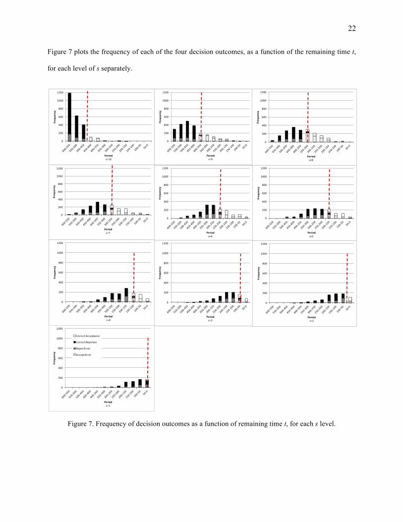
Figure 7 plots the frequency of each of the four decision outcomes, as a function of the remaining time t,

for each level of s separately.

Figure 7. Frequency of decision outcomes as a function of remaining time t, for each s level.

0

200

400

600

800

1000

1200

Freq

uency

Periods=10

0

200

400

600

800

1000

1200

Freq

uency

Periods=9

0

200

400

600

800

1000

1200

Freq

uency

Periods=8

0

200

400

600

800

1000

1200

Freq

uency

Periods=7

0

200

400

600

800

1000

1200

Freq

uency

Periods=6

0

200

400

600

800

1000

1200

Freq

uency

Periods=5

0

200

400

600

800

1000

1200

Freq

uency

Periods=4

0

200

400

600

800

1000

1200

Freq

uency

Periods=3

0

200

400

600

800

1000

1200

Freq

uency

Periods=1

CorrectAcceptance

CorrectRejection

RejectError

AcceptError

0

200

400

600

800

1000

1200

Freq

uency

Periods=2

23

The (dashed) vertical lines in Figure 7 show the threshold periods for the corresponding level of s.

The optimal policy dictates rejections in early periods (on the left hand side of a vertical line) and

acceptances in later periods (on the right hand side of a vertical line). Thus, only correct rejections and

reject errors are possible in early periods, and only correct acceptances and accept errors are possible in

later periods, where the threshold itself decreases in s. Figure 7 makes clear that both types of errors (reject

and accept) tend to become more likely as one gets closer to the threshold period. That is, reject errors

become more likely as t decreases, while accept errors become more likely as t increases, for most s levels.

To make this point formally, we estimate the following two sets of logit regressions (with random effects)

for each s separately:

𝐥𝐨𝐠𝐢𝐭(𝐴𝐸b,/,>) = 𝛽J + 𝛽>𝑡 + 𝜖b + 𝜂b,/,>

𝐥𝐨𝐠𝐢𝐭(𝑅𝐸b,/,>) = 𝛽J + 𝛽>𝑡 + 𝜖b + 𝜂b,/,>

where the dependent variable 𝐴𝐸b,/,> (resp., 𝑅𝐸b,/,>) equals 1 when participant i in round p made an accept

(resp., reject) error at time t, and 0 otherwise.

We summarize estimates of the logit regressions in Table 4. For the reject errors all t coefficients

are negative, and seven of them are significant. This indicates that participants tend to make more (reject)

errors as t decreases. For the accept errors, all t coefficients are positive, and eight of them are significant.

This indicates that participants tend to make fewer (accept) errors as t decreases. Together these results

confirm that participants are more likely to make errors as remaining time (t) is closer to the threshold

period for a particular s level.

One conclusion from our results is that the optimal policy predicts that decision makers will use

fixed thresholds for each s level. However, our experimental results reveal that decision makers do not

strictly adhere to a fixed threshold (policy) as predicted by the optimal policy, and this is a fairly common

behavior across our participants.

24

Table 4. The Results for Logit Regressions. Reject Errors Accept Errors

t Constant Log Likelihood t Constant Log

Likelihood s=1 -0.0076**

(0.0017) 0.0179 (0.3166) -323.59

0.5427 (1.2861)

-24.8778 (12.8165) -7.50

s=2 -0.0076** (0.0015)

0.4836 (0.2871) -404.27

0.0842** (0.0284)

-3.626** (1.0684) -60.05

s=3 -0.0044** (0.0012)

0.3563 (0.3005) -466.22

0.0080 (0.0073)

-1.3472** (0.5363) -111.14

s=4 -0.0050** (0.0012)

0.6103 (0.3466) -518.14

0.0225** (0.0045)

-2.6065 **

(0.5206) -205.91 s=5 -0.0027*

(0.0012) 0.1676 (0.3563) -549.29

0.0107** (0.0027)

-1.887** (0.4148) -256.50

s=6 -0.0020 (0.0012)

-0.1849 (0.4021) -606.68

0.0061** (0.0018)

-1.5936** (0.4066) -333.99

s=7 -0.0020 (0.0013)

-0.4391 (0.5198) -585.52

0.0077** (0.0015)

-1.7324** (0.4027) -399.10

s=8 -0.0029* (0.0014)

-0.2325 (0.6775) -582.15

0.0133** (0.0015)

-3.0287** (0.4679) -440.17

s=9 -0.0023 (0.0014)

-0.5955 (0.7625) -677.35

0.0096** (0.0017)

-1.9801** (0.6106) -292.87

s=10 -0.0079** (0.0017)

2.2048* (1.055) -671.76

0.0103* (0.0047)

-1.2125

(1.814) -56.96 Notes. The standard errors are in parentheses. **p < 0.01; *p < 0.05.

6. Implications of Behavioral Regularities

6.1 Anticipated Regret in Capacity Allocation Decisions

Recall from Section 3 that after our participants allocated their capacity in a season, they were provided

with the following feedback information: the number of units they sold to each of the customer type, their

unused capacity, and the actual demand from each type. In this case, one salient behavioral issue that might

impact participants’ capacity allocation decisions is the feeling of regret. Regret arises when a decision

maker compares the outcome of her decision with that of the alternative decisions that she could have made

(Roese 1994). If an unchosen decision alternative turns out (ex post) to generate a better revenue than the

chosen one, the decision maker will experience some disutility from the forgone revenue. A decision maker

anticipating regret may alter the decision she would make relative to the ones that she would make if she

25

did not have any regret concerns (e.g., Simonson (1992), Zeelenberg et al. (2000), Inman and Zeelenberg

(2002)).

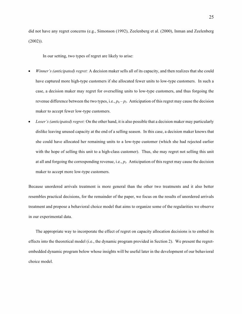
In our setting, two types of regret are likely to arise:

• Winner’s (anticipated) regret: A decision maker sells all of its capacity, and then realizes that she could

have captured more high-type customers if she allocated fewer units to low-type customers. In such a

case, a decision maker may regret for overselling units to low-type customers, and thus forgoing the

revenue difference between the two types, i.e., ph – pl. Anticipation of this regret may cause the decision

maker to accept fewer low-type customers.

• Loser’s (anticipated) regret: On the other hand, it is also possible that a decision maker may particularly

dislike leaving unused capacity at the end of a selling season. In this case, a decision maker knows that

she could have allocated her remaining units to a low-type customer (which she had rejected earlier

with the hope of selling this unit to a high-class customer). Thus, she may regret not selling this unit

at all and forgoing the corresponding revenue, i.e., pl. Anticipation of this regret may cause the decision

maker to accept more low-type customers.

Because unordered arrivals treatment is more general than the other two treatments and it also better

resembles practical decisions, for the remainder of the paper, we focus on the results of unordered arrivals

treatment and propose a behavioral choice model that aims to organize some of the regularities we observe

in our experimental data.

The appropriate way to incorporate the effect of regret on capacity allocation decisions is to embed its

effects into the theoretical model (i.e., the dynamic program provided in Section 2). We present the regret-

embedded dynamic program below whose insights will be useful later in the development of our behavioral

choice model.

26

6.2 A Regret-Embedded Dynamic Program

We modified the boundary conditions of the dynamic program to incorporate the two types of (winner’s

and loser’s) regret which are modeled as the forgone revenue multiplied by the (ex-post) amount that this

forgone revenue is incurred.

Let Rl denote the number of rejected low-type customers, Rh denote the number of rejected high-type

customers;11 Al denote the number of accepted low-type customers at (remaining) time t.12

First of all, note that a decision maker will incur only one type of regret at the end of a season. If she

has unused units, she will regret not selling the units that she could have sold (i.e., the minimum of unused

units and the number of low-class customers she rejected) to low-type customers (loser’s regret). Thus, she

would incur the following psychological cost: [𝑝#min{𝑠, 𝑅#}]. On the other hand, if she sells out, she will

regret forgoing the revenue difference between the two types (i.e., 𝑝" − 𝑝#) for the high-type customers that

she could have captured (i.e., the minimum of number of rejected high-type customers due to not having

any units and the accepted number of low-type customers) if she allocated fewer units to low-type customers

(winner’s regret). Thus, she would incur the following psychological cost: [ 𝑝" − 𝑝# min{𝑅", 𝐴#}].

The resulting regret-embedded dynamic program is given as follows:

𝑉> 𝑠, 𝑅#, 𝑅", 𝐴# =

• 1 − 𝜆" − 𝜆# 𝑉>+,(𝑠, 𝑅#, 𝑅", 𝐴#) + 𝜆" 𝑝" + 𝑉>+,(𝑠 − 1, 𝑅#, 𝑅", 𝐴#) +

𝜆#max𝑝# + 𝑉>+,(𝑠 − 1, 𝑅#, 𝑅", 𝐴# + 1)

𝑉>+,(𝑠, 𝑅# + 1, 𝑅", 𝐴#) , for𝑡 = 1, 2, … , 𝑇, and𝑠 ≥ 1;

11 Note that one should never reject a high-class customer, thus Rh is the number of high-class customers who arrive after the firm sells all of its capacity. 12 We shorthand the notations for Rl, Rh, and Al, rather than using Rl(t), Rh(t), and Al(t), similar to the notation of s.

27

• 1 − 𝜆" − 𝜆# 𝑉>+,(𝑠, 𝑅#, 𝑅", 𝐴#) + 𝜆"𝑉>+, 𝑠, 𝑅#, 𝑅" + 1, 𝐴# + 𝜆#𝑉>+,(𝑠, 𝑅# + 1, 𝑅", 𝐴#)

, for𝑡 = 1, 2, … , 𝑇, and𝑠 = 0;

with boundary condition

𝑉J 𝑠, 𝑅#, 𝑅", 𝐴# = −α’ (𝑝" − 𝑝#) min{𝑅", 𝐴#} –β’ 𝑝# min{𝑠, 𝑅#} , for𝑡 = 0, and𝑠 ≥ 0;

where α’ and β’ allow decision makers to evaluate the psychological costs resulting from winner’s and

loser’s regret differently.

In addition to the original state variables of t and s, we have three more variables, namely Rl, Rh,

and Al, to define a state in the new model. Now, the value function 𝑉> 𝑠, 𝑅#, 𝑅", 𝐴# indicates the decision

maker’s expected future utility (including non-monetary (dis)utilities) when there are s units on hand, 𝑅# of

low-type customers have been rejected, 𝑅" of high-type customers have been rejected, and 𝐴# of low-type

customers have been accepted so far, and t time intervals remaining until the end of the selling season.

Recall that, 𝜆" and 𝜆# denote the arrival probabilities for high-type and low-type customers respectively,

and 𝑝" and 𝑝# denote high price and low price, respectively.

The following insight of the regret-embedded model is worth highlighting. Standard theoretical

model indicates that a decision maker will make a decision for a low-type customer based on remaining

time (t) and remaining units (s). The regret-embedded theoretical model indicates that in addition to these

two (t and s), a decision maker anticipating regret will consider the number of accepted low-type customers

(𝐴#) and the number of rejected low-type customers (𝑅#) thus far, while making an accept or reject decision

for a low-type customer. We use this insight and check whether these two variables affect participants’

capacity allocation decisions.

28

6.3 A Behavioral Choice Model

In this section, for the unordered arrivals problem, we propose a behavioral choice model which

incorporates the decision noise and the effect of the two variables (𝑅# and 𝐴#)identified by our regret-

embedded dynamic program. Specifically, the behavioral choice model aims to organize the following

regularities:

1. Regret feelings have an effect on participants’ capacity allocation decisions.

2. Decision makers make more errors (either accept or reject) as they get closer to the threshold periods,

i.e., as the expected utility of accepting and rejecting a low-type customer become closer.

3. Decision makers do not strictly adhere to a fixed threshold policy.

The underlying idea of this choice model is similar to Bearden and Murphy (2007) and to Palley and

Kremer (2014).

Recall that under the standard theoretical model, a decision maker accepts a low-type customer if 𝑝# +

𝑉>+,?+, ≥ 𝑉>+,? , i.e., utility of accepting this customer is at least as high as the utility of rejecting it. We first

incorporate decision noise into the utility values for accept and reject decisions for a low-type customer.

To this end, we add a random element to the choice rule which captures the idea that, due to limited

cognitive abilities, decision makers are prone to errors (Loomes et al. 2002). These random errors account

for a variety of unmodeled factors such as the decision maker may not be able to assess the expected values

of each available option (i.e., either accept or reject a low-class customer), or she may make mistakes while

comparing these expected values. Thus, we assume that a decision maker accepts a low-type customer if

𝑝# + 𝑉>+,?+, + mno≥ 𝑉>+,? + mp

o, where 𝜀, and 𝜀rare assumed to be independent standard Gumbel random

variables (therefore 𝜀 = 𝜀,- 𝜀r is a logistic random variable) and γ>0 measures the degree of noise, and as

γ grows to infinity, the decision maker makes perfectly rational decisions, whereas if γgoes to zero the

29

decision maker randomizes between accept and reject decisions. Under this model the choice probability

for accepting a low-type customer is given by:

Pr(𝐴𝑐𝑐𝑒𝑝𝑡) = 𝑒o(uvwwxyz)

𝑒o(uvwwxyz) + 𝑒o(u{x|xwz)=

𝑒o(/0}~z�n��n}mno )

𝑒o(/0}~z�n��n}mno ) + 𝑒o(~z�n

� }mpo )

The central idea of this concept is that decision maker does not always choose the utility

maximizing alternative, but the more attractive option is chosen more frequently. Note that incorporating

decision noise into the utility values results in varying thresholds rather than assuming a fixed threshold for

a given level of s for the decision maker. Once we consider the effects of decision noise, we can now

investigate the effects of other potential biases on the behavior which is the effect of regret in our case.

To add regret, we add the variables 𝑅# and 𝐴# with additional regret parameters into the utility

values. As a result, we obtain the following (full) model:

• Model 1 (Full Model): Noisy Utilities & Regret

𝜑� 𝑡, 𝑠, 𝑝#, 𝐴#, 𝑅#, 𝛼, 𝛽, 𝛾 =Accept, if𝑝# + 𝑉>+,?+, − 𝛼𝐴# +

𝜀,𝛾≥ 𝑉>+,? − 𝛽𝑅# +

𝜀r𝛾;

Reject,otherwise.

Note that when we set the coefficients of regret parameters (α and β) to zero in full model, we recover the

(reduced) model which incorporates noise only.

• Model 2 (Reduced Model): Noisy Utilities

𝜑� 𝑡, 𝑠, 𝑝#, 𝛾 =Accept, if𝑝# + 𝑉>+,?+, +

𝜀,𝛾≥ 𝑉>+,? +

𝜀r𝛾;

Reject,otherwise.

Then, we estimate a logit model to see the effect of regret on participants’ decisions. We report the

estimation results in Table 5 below.

30

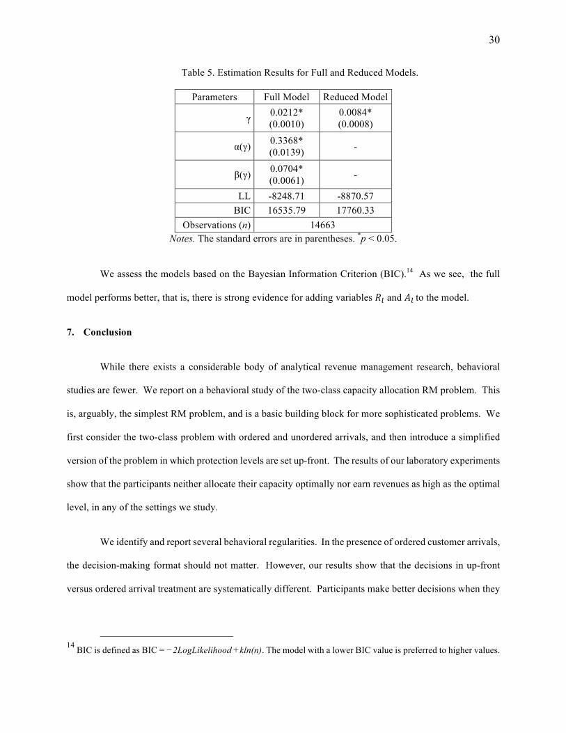
Table 5. Estimation Results for Full and Reduced Models.

Parameters Full Model Reduced Model

γ 0.0212* (0.0010)

0.0084* (0.0008)

α(γ) 0.3368* (0.0139) -

β(γ) 0.0704* (0.0061) -

LL -8248.71 -8870.57 BIC 16535.79 17760.33

Observations (n) 14663 Notes. The standard errors are in parentheses. *p < 0.05.

We assess the models based on the Bayesian Information Criterion (BIC).14 As we see, the full

model performs better, that is, there is strong evidence for adding variables 𝑅# and 𝐴#to the model.

7. Conclusion

While there exists a considerable body of analytical revenue management research, behavioral

studies are fewer. We report on a behavioral study of the two-class capacity allocation RM problem. This

is, arguably, the simplest RM problem, and is a basic building block for more sophisticated problems. We

first consider the two-class problem with ordered and unordered arrivals, and then introduce a simplified

version of the problem in which protection levels are set up-front. The results of our laboratory experiments

show that the participants neither allocate their capacity optimally nor earn revenues as high as the optimal

level, in any of the settings we study.

We identify and report several behavioral regularities. In the presence of ordered customer arrivals,

the decision-making format should not matter. However, our results show that the decisions in up-front

versus ordered arrival treatment are systematically different. Participants make better decisions when they

14 BIC is defined as BIC = −2LogLikelihood +kln(n). The model with a lower BIC value is preferred to higher values.

31

make an up-front decision rather than sequential decisions for the entire capacity. Similar to the ordered

arrivals treatment, decision making is also sequential in the unordered arrivals treatment. In theory, making

an upfront decision results in sub-optimal solution to the unordered arrivals problem, so we might expect

the performance to suffer when decisions are made up-front rather than sequential. We find that up-front

decision making results in higher revenues than sequential decision making (although the difference is not

significant).

However, an implication of this finding is that there is room for improving decision making process

in a dynamic (unordered arrivals) setting, because making an up-front decision is a substantial

simplification for this setting, because it requires the update of the decisions based on remaining time and

remaining inventory level. The main insight from these results is that decision makers do not perform well

when they are faced with sequential decisions.

In the presence of ordered arrivals (ordered arrivals and up-front treatments), we observe that

participants set their protection levels between optimal and mean of high-type demand. We mentioned that

ordered arrivals and up-front treatment are mathematically equivalent to the newsvendor problem. One

ancillary observation we can make is that we find that pull-to-center bias—reported by behavioral studies

of the newsvendor problem—persists in RM decisions, so behavior in the ordered arrivals two-class RM

problem shares qualitative regularities with the behavior in the newsvendor problem. Thus, our results

affirm that the results of newsvendor are somewhat robust to the decision making frame in operations

management contexts (i.e., revenue management vs. inventory decisions). One implication of this finding

is that the newsvendor results documented in behavioral operations literature might be helpful to

understand, and even improve, the decision making performance in capacity allocation decisions. Our

results also imply that the decision making format (up-front vs. sequential) may matter for the newsvendor

problem.

32

In the presence of unordered arrivals, we observe the following regularities in participants’

behavior: Decision makers do not strictly adhere to a fixed threshold (policy) as prescribed by the optimal

policy. They make more errors as they get closer the threshold periods. Inspired by these observations, we

propose an alternative model that incorporates the decision noise and regret feelings of participants, and

organizes our experimental data better.

Our study reports on several shortcomings of the decision making process in RM decisions.

Overall, we believe that the insights of this study can serve to understand and improve decision making

performance of RM managers. There are a number of promising avenues for future research. First, we

take for granted that demand for each customer segment is independent of the (capacity) controls being

applied by the firm. That is, a denied customer will not upgrade to a high-type (i.e., buy-up), or she will

not downgrade to a low-type (i.e., buy-down) and is simply lost. Incorporating buy-down and/or buy-up

behavior can have important consequences on the revenues, and thus seems worthwhile to examine. In

addition, understanding how competition affects RM decisions, when human decision makers are involved,

would be quite helpful for firms. Thus, looking into a model in which two (or more) firms with similar

product offerings (e.g., two restaurants offering the same cuisine with comparable food quality and prices)

compete for customers is another fruitful direction for future research.

References

Bassok, Y., R. Ernst. 1995. Dynamic Allocations for Multi-Product Distribution. Transportation Science. 29(3), 256-266.

Bearden, J. N., R. O. Murphy. 2007. On Generalized Secretary Problems. Abdellaoui M., R. D. Luce, M. J. Machina, B. Munier, eds. Uncertainty and Risk: Mental, Formal and Experimental Representation. Springer, New York, 187–206.

Bearden, J. N., R. O. Murphy, A. Rapoport. 2008. Decision Biases in Revenue Management: Some Behavioral Evidence. Manufacturing and Service Operations Management. 10(4), 625-636.

Belobaba, P. P. 1989. Application of a Probabilistic Decision Model to Airline Seat Inventory Control. Operations Research. 37(2), 183-197.

Bendoly, E. 2011. Linking Task Conditions to Physiology and Judgment Errors in RM Systems. Production and Operations Management. 20(6), 860-876.

Brumelle, S. L., J. I. McGill. 1993. Airline Seat Allocation with Multiple Nested Fare Classes. Operations Research. 41, 127-137.

33

Curry, R. E. 1990. Optimal Airline Seat Allocation with Fare Classes Nested by Origins and Destinations. Transportation Science. 24, 193-204.

Diecidue, E., N. Rudi, W. Tang. 2012. Dynamic Purchase Decisions under Regret: Price and Availability. Decision Analysis. 9(1), 22-30. Donovan, A. W. 2005. Yield Management in the Airline Industry. The Journal of Aviation/Aerospace

Education and Research. 14(3), 11-19. Engelbrecht-Wiggans, R., E. Katok. 2007. Regret in Auctions: Theory and Evidence. Economic Theory. 33(1), 81-101. Fischbacher, U. 2007. z-Tree: Zurich Toolbox for Ready-made Economic Experiments. Experimental

Economics. 10(2), 171-178. Gerchak, Y., M. Parlar, T. K. M. Lee. 1985. Optimal Rationing Policies and Production Quantities for

Products with Several Demand Classes. Canadian Journal of Administrative Sciences. 2, 161-176.

Greiner, B. 2004. The Online Recruitment System ORSEE 2.0 - A Guide for the Organization of Experiments in Economics. University of Cologne, Working Paper Series in Economics 10.

Hendel, I., A. Nevo. 2006. Measuring the Implications of Sales and Consumer Inventory Behavior. Econometrica, 74(6), 1637-1673.

Inman, J., M. Zeelenberg. 2002. Regret in Repeat Purchase versus Switching Decisions: The Attenuating Role of Decision Justifiability. Journal of Consumer Research. 29(1) 116-128. Katok, E. 2011. Using Laboratory Experiments to Build Better Operations Management Models.

Foundations and Trends in Technology, Information and Operations Management. 5(1), 1-86. Kimes, S. E. 2003. Revenue Management: A Retrospective. Cornell Hotel and Restaurant Administration

Quarterly. 44, 131-138. Kocabıyıkoğlu, A., C. I. Göğüş, M. S. Gönül. 2015. Revenue Management vs. Newsvendor Decisions:

Does Behavioral Response Mirror Normative Equivalance? Production and Operations Management. 24(5), 750-761.

Kremer, M, B. Mantin, A. Ovchinnikov. 2013. Strategic Customers, Myopic Retailers. Working Paper, Darden Business School, University of Virginia, Charlottesville.

Lautenbacher, C., S. Stidham. 1999. The Underlying Markov Decision Process in the Single-Leg Airline Yield Management Problem. Transportation Science. 33(2), 136-146.

Lee, T. C., M. Hersh. 1993. A Model for Dynamic Airline Seat Inventory Control with Multiple Seat Bookings. Transportation Science. 27, 252-265.

Li, J., N. Granados, S. Netessine. 2011. Are Consumers Strategic? Structural Estimation from the Air-Travel Industry. Working Paper.

Littlewood, K. 1972. Forecasting and Control of Passenger Bookings. Proceedings of AGIFORS 12th Annual Symposium. 95-128.

Loomes, G., P. G. Moffat, R. Sugden. 2002. A Microeconometric Test of Alternative Stochastic Theories of Risky Choice. Journal of Risk and Uncertainty. 24, 103–130.

Mak, V., A. Rapoport, E. J. Gisches. 2012. Competitive Dynamic Pricing with Alternating Offers Theory and Experiment. Games Economic Behavior. 75(1), 250-264.

Nasiry, J., I. Popescu. 2012. Advance Selling when Consumers Regret. Management Science. 58(6), 1160-1177.

Nair, H. 2007. Intertemporal Price Discrimination with Forward-Looking Consumers: Application to the US Market for Console Video-Games. Quantitative Marketing and Economics. 5(3), 239-292.

Osadchiy, N., E. Bendoly. 2011. Are Consumers Really Strategic? Implications from an Experimental Study. Working paper, Emory University, Atlanta, GA.

Özer, Ö., R. Phillips. 2012. (Eds.), The Oxford Handbook of Pricing Management. Oxford University Press, London.

Özer, Ö., Y. Zheng. 2016. Markdown or Everyday-Low-Price? The role of behavioral motives. Management Science. 62(2), 326-346.

34

Palley, A. B., M. Kremer. 2014. Sequential Search and Learning from Rank Feedback: Theory and Experimental Evidence. Management Science. 60, 2525-2542.

Papastavrou, J. D., S. Rajagopalan, A. J. Kleywegt. 1996. The Dynamic and Stochastic Knapsack Problem with Deadlines. Management Science. 42, 155-172.

Perakis, G., G. Roels. 2008. Regret in the Newsvendor Model with Partial Information. Operations Research. 56(1) 188–203.

Roese, N. 1994. The Functional Basis of Counterfactual Thinking. Journal of Personality and Social Psychology. 66(5) 805-818.

Robinson, L. W. 1995. Optimal and Approximate Control Policies for Airline Booking with Sequential Nonmonotonic Fare Classes. Operations Research. 43, 252-263.

Siegel, S. 1965. Nonparametric Statistics for the Behavioral Sciences. Wiley, New York. Simonson, I. 1992. The Influence of Anticipating Regret and Responsibility on Purchase Decisions. Journal of Consumer Research. 19(1) 105-118. Talluri, K. T. 2012. Revenue Management. Ö Özer, R. Phillips, eds. The Oxford Handbook of Pricing

Management. Oxford University Press, Oxford, UK, Chapter 26. Talluri, K. T., G. J. Van Ryzin. 2004. The Theory and Practice of Revenue Management. Kluwer

Academic Publishers, Norwell, MA. Wollmer, R. 1992. An Airline Seat Management Model for a Single Leg Route when Lower Fare Classes

Book First. Operations Research. 40, 26-37. Zeelenberg, M., W. van Dijk, A. Manstead, J. van der Pligt. 2000. On Bad Decisions and Disconfirmed

Expectancies: The Psychology of Regret and Disappointment. Cognition and Emotion. 14(4) 521-541.

Appendix

A. Sample Instructions for the Unordered Arrivals Treatment

General. The purpose of this session is to study how people make decisions in a particular situation. If you have any questions, feel free to raise your hand and a monitor will assist you. From now until the end of the session, please do not communicate with other participants in the room.

During the session, you will play a game from which you can earn ‘Experimental Currency Units (ECUs)’. The ECUs you earn will be converted into U.S. dollars at a rate of 3000 ECUs per $1. Upon completion of the game, you will be paid your total earnings in U.S. cash plus a $5 show-up fee.

Description of the game. You are a manager at a company that sells tickets for an upcoming event (e.g., Broadway show). You have 10 tickets to sell, in total. There are two types of customers: low-revenue from whom you earn 20 ECUs, or high-revenue from whom you earn 200 ECUs. Each customer demands one unit. Each round of the game consists of 600 periods. In each period, a low-revenue customer arrives with probability Pr(Low) = 0.0244, or a high-revenue customer arrives with probability Pr(High) = 0.0083, but both customers cannot arrive in the same period. This indicates that the probability of no customer arrives in a period is Pr(No customer) = 0.9673. The probability distributions for the total number of each type of customers for a round are also shown on a separate page.

35

The total number of high-revenue and the total number of low-revenue customers in any round are independent from each other. Also, the total number of high-revenue and the total number of low-revenue customers for any one round are independent of the demand from other rounds. Thus, a small or large demand in a round has no influence on whether demand is small or large in other rounds. In each round of the game, when a customer arrives, you decide whether to accept or reject this demand. • The maximum revenue that you can earn from any customer is high-revenue (i.e., 200 ECUs). Thus,

you never reject a high-revenue customer as long as you have available capacity left.

• Whenever a low-revenue customer arrives, you need to decide whether to accept or reject this customer. If you accept too many low-revenue customers, you sell the units at low-revenue instead of selling them at high-revenue, thus lose 180 ECUs per unit (the difference between high-revenue and low-revenue). If you accept too few low-revenue customers, you may have unsold units at the end and forego 20 ECUs per unit (low-revenue).

Overall for a round, you need to decide when to accept or reject low-revenue customers. Your goal is to maximize the total revenue. Calculating revenue. For each round, computer generates random low-revenue and high-revenue demands. When a customer arrives, if you accept this demand you earn its associated revenue; if you reject it, then you simply earn 0 ECU. Assume that, overall for a round, you have accepted y units of low-revenue customers, then your revenue for this round is calculated as follows:

Revenue = 200 ´ min{10 - y, High-demand} + 20 ´ y For example, suppose you accept 6 low-revenue customers for a round. This indicates that you can sell at most 4 units to high-revenue customers.

o Assume that the high-demand is 5, then your revenue for this round is: 200 ´ min{4, 5} + 20 ´ 6 = 920 ECUs.

o Now, assume that the high-demand is 2, then your revenue for this round is:

200 ´ min{4, 2} + 20 ´ 6 = 520 ECUs. Note that when the demand for a high-revenue customer turns out to be lower than the remaining capacity not used for low-revenue customers, you lose revenue opportunities for sale of this capacity. Information to help you in your decision. A pen and blank sheet of paper have been provided for any calculations or notes you might wish to make.

In a period, whenever a customer arrives, you will be provided information on (i) the remaining periods in this round, (ii) how much capacity you have allocated to each of the high-revenue and low-revenue customers thus far in current round, and (iii) your current revenue in this round. At the end of each round, the computer will display the history of play (how much capacity you allocated to each of the customers, the realized high-revenue and low-revenue demands, the unsold capacity you had, and your resulting total revenue) for each round.

Number of rounds. The game lasts for 40 rounds.

36

Consent Forms. If you wish to participate in this study, please read the accompanying consent form prior to beginning the game.

Demand Distribution Information

37

B. Sample Screenshots for the Unordered Arrivals Treatment

C. Acceptance - Rejection Time Analysis for a Low-Class Customer for Each Capacity Level “s”

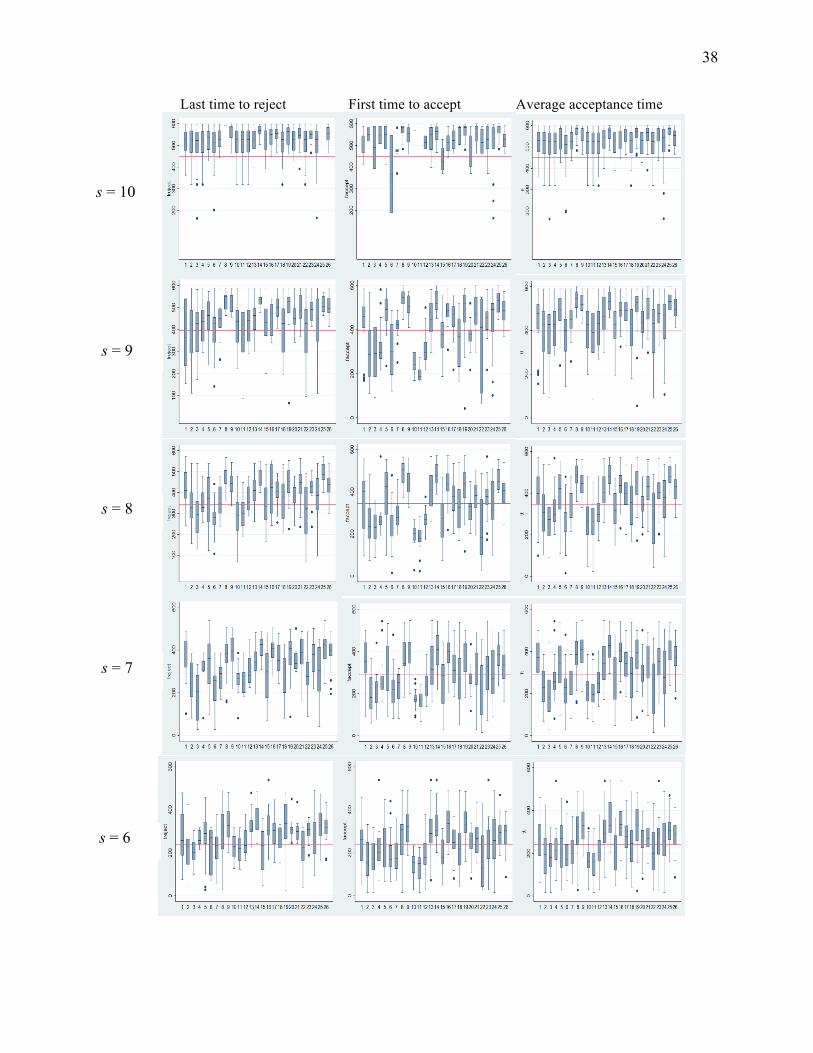
Figure below displays the frequency distributions of the acceptance time for a low-class customer with regard to the optimal acceptance time, for each s level separately. The distributions are shown by remaining units s (row), last time to reject / first time to accept / average acceptance time (by taking the average of last time to reject and first time to accept) a low-class customer (column), and subject (box plot). The bottom and top edges of each box are located at 25th and 75th percentiles of the sample. The vertical lines extend from the box as far as the data extend, to a distance of at most 1.5 interquartile range. Any value that is more extreme than this is marked by a dot. The reference line is drawn horizontally at the optimal time to start accepting a low-class customer.

38

Last time to reject First time to accept Average acceptance time

s = 10

s = 9

s = 8

s = 7

s = 6

39

s = 5

s = 4

s = 3

s = 2

s = 1