Causal discovery, Bayesian networks, and structural equation models

A Bayesian Theory of Sequential Causal Learning and Abstract Transfer
Hongjing Lu 1,2, Randall R. Rojas 3, Tom Beckers 4,5, Alan L. Yuille 1,2
1 Department of Psychology, University of California, Los Angeles 2 Department of Statistics, University of California, Los Angeles 3 Department of Economics, University of California, Los Angeles 4 Department of Psychology, KU Leuven 5 Department of Clinical Psychology and Amsterdam Brain and Cognition,
University of Amsterdam
Corresponding author: Hongjing Lu
Department of Psychology
University of California, Los Angeles
405 Hilgard Ave.
Los Angeles, CA 90095-1563
Email: [email protected]
Keywords: Causal learning, Sequential causal inference, Bayesian inference, Abstract transfer, Model selection, Blocking
2
Abstract
Two key research issues in the field of causal learning are how people acquire causal knowledge
when observing data that are presented sequentially, and the level of abstraction at which
learning takes place. Does sequential causal learning solely involve the acquisition of specific
cause-effect links, or do learners also acquire knowledge about abstract causal constraints?
Recent empirical studies have revealed that experience with one set of causal cues can
dramatically alter subsequent learning and performance with entirely different cues, suggesting
that learning involves abstract transfer, and such transfer effects involve sequential presentation
of distinct sets of causal cues. It has been demonstrated that pre-training (or even post-training)
can modulate classic causal learning phenomena such as forward and backward blocking. To
account for these effects, we propose a Bayesian theory of sequential causal learning. The
theory assumes that humans are able to consider and use several alternative causal generative
models, each instantiating a different causal integration rule. Model selection is used to decide
which integration rule to use in a given learning environment in order to infer causal knowledge
from sequential data. Detailed computer simulations demonstrate that humans rely on the
abstract characteristics of outcome variables (e.g., binary versus continuous) to select a causal
integration rule, which in turn alters causal learning in a variety of blocking and overshadowing
paradigms. When the nature of the outcome variable is ambiguous, humans select the model that
yields the best fit with the recent environment, and then apply it to subsequent learning tasks.
Based on sequential patterns of cue-outcome co-occurrence, the theory can account for a range
of phenomena in sequential causal learning, including various blocking effects, primacy effects
in some experimental conditions, and apparently abstract transfer of causal knowledge.

3
1. Introduction
The study of causality has traditionally been a central topic in philosophy, where
causality has even been dubbed the "cement of the universe" (Mackie, 1974). In the past quarter
century, researchers in the fields of human and animal cognition have built computational
theories of how various intelligent organisms, ranging from rats to humans, can acquire
knowledge about cause-effect relations. This work has been guided in part by advances in the
application of probabilistic Bayesian models to account for causal learning (Griffiths &
Tenenbaum, 2005, 2009; Holyoak, Lee, & Lu, 2010; Lu, Yuille, Liljeholm, Cheng, & Holyoak,
2006, 2008a; for a review see Holyoak & Cheng, 2011). However, most theoretical work on
human causal learning has focused on the induction of causal knowledge from summary data—
situations in which all causal observations are presented simultaneously and processed at once.
In real life, observers must often cope with data that are presented sequentially, making interim
decisions that are subject to revision as additional data become available.
Studies of human performance on sequential data, as well as conditioning experiments
with rats and other non-human animals (which by necessity involve sequential data), show that
the order of data presentation can dramatically influence causal learning. An example is the
classic blocking effect: learning that cue A alone repeatedly produces an outcome or effect
(represented as A+ training) reduces the perceived causal efficacy of a second, redundant cue X
that is compounded with A and repeatedly paired with a positive outcome (AX+ trials). Blocking
can be obtained either in the forward direction, A+ trials followed by AX+ trials (Dickinson,
Shanks, & Evenden, 1984; Kamin, 1969; Vandorpe & De Houwer, 2005), or in the backward
direction, A+ trials preceded by AX+ trials (De Houwer, Beckers, & Glautier, 2002; Miller &
Matute, 1996; Shanks, 1985; Sobel, Tenenbaum, & Gopnik, 2004). However, the magnitude of
4
the blocking effect often differs between forward and backward experiments, indicating that
learning of causal knowledge can depend on the temporal order in which information is
presented (see also Dennis & Ahn, 2001; Danks & Schwartz, 2006).
The present paper presents a computational theory to account for a range of phenomena
in human sequential causal learning. The theory has two major components. (1) A dynamic
model based on a Bayesian framework is used to update causal briefs, i.e., the strength that a
cause generates or prevents an effect, in a trial-by-trial manner. This model deals with sequential
data and enables the use of multiple causal integration rules, each rule specifying a distinct way
in which the influences of multiple causes are combined to determine the outcome variable (i.e.,
their common effect). (2) The theory introduces a learning mechanism that enables transfer of
abstract causal knowledge from one situation to another even when the specific causal cues are
entirely different (i.e., an account for abstract causal transfer). In other words, we propose that
individual causal inferences are not made in isolation. Instead, a causal model is selected at an
abstract level based on alternative integration rules; the selected model will then be used to
estimate the cause-effect relations relevant to subsequent data.
In Section 2, we present an overview of the modeling issues that arise in sequential causal
learning. In Section 3, a Bayesian sequential learning model is introduced that allows the use of
multiple causal integration rules. We focus on the key conceptual components of the theory;
mathematical derivations are provided in the Appendix, as are details of the implementation used
in our simulations. Section 4 reviews a set of experimental findings with binary outcome
variables, which compares model simulations with different integration rules. We present
simulation results showing that the proposed theory, which includes a set of different causal
generative models, accounts for a range of blocking effects in the literature, and also provides an
5
explanation of some important differences in the performance of humans in sequential causal
learning tasks as compared to rats in conditioning paradigms. In Section 5, we review abstract
transfer effects in causal learning, and show how our framework can be extended to select
between alternative causal models so as to account for such effects. In Section 6 we review
empirical evidence for primacy effects in causal learning (i.e., the phenomenon that final causal
judgments are often more strongly influenced by information presented early), extend the model
by allowing the learning rate to vary over time, and report simulation results that account for the
qualitative trend of this phenomenon. Section 7 provides a summary and general discussion. In
the present paper, all empirical studies presented sequential data in a trial-by-trial display.
2. Overview of Modeling Issues in Sequential Causal Learning
2.1 Causal Integration Rules for Causal Learning
Causal influence from an individual cue can be measured as causal power (Cheng, 1997),
the probability with which this cue actually causes an effect. When multiple causes co-occur
with the effect, causal integration rules are needed to combine causal powers from individual
cues to determine the probability of the occurrence of the effect. Research on causal learning
has yielded evidence that humans are able to learn multiple causal integration rules (Lucas &
Griffiths, 2010; Waldmann, 2007; see also Griffiths & Tenenbaum, 2009). Although ample
evidence supports the existence of multiple causal integration rules in reasoning, computational
models have primarily focused on causal learning in experiments where contingency data are
presented in a summary format. For modeling sequential causal learning, a coherent framework
is needed to incorporate different integration rules. We first review different causal integration
rules in the literature, and Section 3 will present a framework that enables sequential causal
learning with different integration rules. The present paper considers three alternative rules to
6
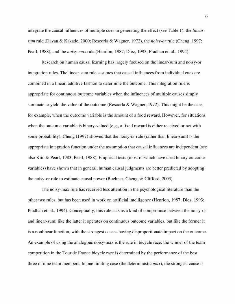
integrate the causal influences of multiple cues in generating the effect (see Table 1): the linear-
sum rule (Dayan & Kakade, 2000; Rescorla & Wagner, 1972), the noisy-or rule (Cheng, 1997;
Pearl, 1988), and the noisy-max rule (Henrion, 1987; Diez, 1993; Pradhan et. al., 1994).
Research on human causal learning has largely focused on the linear-sum and noisy-or
integration rules. The linear-sum rule assumes that causal influences from individual cues are
combined in a linear, additive fashion to determine the outcome. This integration rule is
appropriate for continuous outcome variables when the influences of multiple causes simply
summate to yield the value of the outcome (Rescorla & Wagner, 1972). This might be the case,
for example, when the outcome variable is the amount of a food reward. However, for situations
when the outcome variable is binary-valued (e.g., a fixed reward is either received or not with
some probability), Cheng (1997) showed that the noisy-or rule (rather than linear-sum) is the
appropriate integration function under the assumption that causal influences are independent (see
also Kim & Pearl, 1983; Pearl, 1988). Empirical tests (most of which have used binary outcome
variables) have shown that in general, human causal judgments are better predicted by adopting
the noisy-or rule to estimate causal power (Buehner, Cheng, & Clifford, 2003).
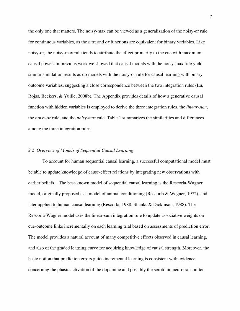
The noisy-max rule has received less attention in the psychological literature than the
other two rules, but has been used in work on artificial intelligence (Henrion, 1987; Diez, 1993;
Pradhan et. al., 1994). Conceptually, this rule acts as a kind of compromise between the noisy-or
and linear-sum: like the latter it operates on continuous outcome variables, but like the former it
is a nonlinear function, with the strongest causes having disproportionate impact on the outcome.
An example of using the analogous noisy-max is the rule in bicycle race: the winner of the team
competition in the Tour de France bicycle race is determined by the performance of the best
three of nine team members. In one limiting case (the deterministic max), the strongest cause is
7
the only one that matters. The noisy-max can be viewed as a generalization of the noisy-or rule
for continuous variables, as the max and or functions are equivalent for binary variables. Like
noisy-or, the noisy-max rule tends to attribute the effect primarily to the cue with maximum
causal power. In previous work we showed that causal models with the noisy-max rule yield
similar simulation results as do models with the noisy-or rule for causal learning with binary
outcome variables, suggesting a close correspondence between the two integration rules (Lu,
Rojas, Beckers, & Yuille, 2008b). The Appendix provides details of how a generative causal
function with hidden variables is employed to derive the three integration rules, the linear-sum,
the noisy-or rule, and the noisy-max rule. Table 1 summarizes the similarities and differences
among the three integration rules.
2.2 Overview of Models of Sequential Causal Learning
To account for human sequential causal learning, a successful computational model must
be able to update knowledge of cause-effect relations by integrating new observations with
earlier beliefs. 1 The best-known model of sequential causal learning is the Rescorla-Wagner
model, originally proposed as a model of animal conditioning (Rescorla & Wagner, 1972), and
later applied to human causal learning (Rescorla, 1988; Shanks & Dickinson, 1988). The
Rescorla-Wagner model uses the linear-sum integration rule to update associative weights on
cue-outcome links incrementally on each learning trial based on assessments of prediction error.
The model provides a natural account of many competitive effects observed in causal learning,
and also of the graded learning curve for acquiring knowledge of causal strength. Moreover, the
basic notion that prediction errors guide incremental learning is consistent with evidence
concerning the phasic activation of the dopamine and possibly the serotonin neurotransmitter

8
systems during learning (Daw, Courville, & Dayan, 2007; Montague, Dayan, & Sejnowski,
1996; Yu & Dayan, 2005).
However, despite its attractive features, the Rescorla-Wagner model faces a number of
severe difficulties. First, it is unable to account for retroactive effects on strength judgments,
such as backward blocking effects (De Houwer et al., 2002; Shanks, 1985). Second, the model
does not provide an account of how people (or animals) code uncertainty of causal strength
estimates. For example, the model cannot distinguish between lack of knowledge about the
causal efficacy of a cue and certainty that the cue is ineffective, as both situations will yield a
strength estimate of zero (Dayan & Yu, 2003; Holyoak & Cheng, 2011).
A more sophisticated sequential model was developed by Dayan and his colleagues
(Daw, et al., 2007; Dayan & Kakade, 2000; Dayan, Kakade, & Montague, 2000; Dayan & Long,
1998). This probabilistic model accommodates the learner’s uncertainty by updating full
probability distributions of causal strengths, rather than simply point estimates. Within a
Bayesian framework, this model is able to handle retroactive effects and influences of trial order,
such as differences between forward versus backward blocking, which are beyond the capacity
of the Rescorla-Wagner model.
However, problems arise in extending the model to human causal learning, especially
with binary outcome variables. The sequential model developed by Dayan and colleagues
(Dayan & Kakade, 2000), assumes a particular integration rule, the linear-sum, according to
which the net influence of multiple causes on their common effect is simply the additive sum of
their individual influences. The choice of the linear-sum rule was partly motivated by
computational convenience. When the distributions of key parameters, such as causal weights,
are assumed to follow Gaussian distributions, the linear-sum rule enables incremental updating

9
with analytic solutions implemented by a Kalman filter, a technique adopted from engineering
applications (Anderson & Moore, 1979; Kalman, 1960; Meinhold & Singpurwalla, 1983). In this
case, the model implementation is easy for just updating the means and variances of the posterior
distributions. But as Daw et al. (2008, p. 430) recognize, “…the Gaussian form of the output
model… is only appropriate in rather special circumstances…. For instance, if the outcome is
binary rather than continuous, as in many human experiments, it cannot be true.” Hence, a
computational framework is needed to incorporate different causal integration rules for inferring
the cause-effect relations from sequential data.
3. A Bayesian Sequential Model with Alternative Integration Rules
We propose a computational theory including a sequential model to incorporate multiple
causal integration rules for inferring cause-effect relations, and a model selection procedure to
choose appropriate causal integration rules for subsequent inferences. As noted earlier, the theory
proposed in the present paper incorporates three alternative rules for integrating the causal
influences of multiple cues in generating an outcome: the linear-sum, noisy-or, and noisy-max
rules (see Table 1). Given a specific causal integration rule, Bayesian sequential learning updates
the probability distribution of the causal weights over time. Each update depends on all the data
D up to time t, defined as Dt . The cues x correspond to binary values indicating the presence or
absence of cues, whereas the outcome O can take either binary or continuous values. As
illustrated in Figure 1, under a causal generative model (m) based on a specific integration rule,
the distribution of causal weights, , is updated with two steps applied iteratively (Ho & Lee,
1964; Meinhold & Singpurwalla, 1983): (1) at time t, a prediction step infers an expected
distribution of causal weights in the next trial; and (2) at time t+1 with observed data Dt+1, a

10
correction step applies Bayes rule to update the distribution of causal weights by combining the
prediction and the new data:
| , | | , ,
| , | , | ,
| ,.
==========================================================
Insert figure 1 here
==========================================================
The proposed Bayesian sequential learning model is driven by prediction errors and
uncertainty over time. For example, if a sequence of observations indicates that eating a fruit and
breaking out in a rash co-occur (i.e., A+ trials), then the model would predict that the probability
of a rash will be higher after eating the fruit. If the observation on the next trial is consistent with
the prediction, the peak of the probability distribution of causal weights will shift toward greater
values of causal strength, and the variance of estimated causal weights will decrease to indicate
more certainty. However, if the observation on the sixth trial disagrees with the prediction, the
peak of the distribution would shift toward lower causal weights, and the associated variance
would increase.
The Bayesian sequential learning model provides a way for solving the sequential
parameter-updating problem for any form of causal integration rule. A special case of a Bayesian
sequential learning model is the Kalman filter approach used by Dayan et al. (2000), in which the
likelihood function of the sequential model is defined by Gaussian distributions and the linear-

11
sum rule for causal integration. The general Bayesian sequential learning approach adopted here
overcomes this restriction, thereby allowing our theory to model the full range of integration
rules relevant to human causal learning.
Because there is no analytic solution for a Bayesian sequential learning model when
adopting non-Gaussian distributions for the likelihood function and using causal integration rules
other than the linear-sum, we implemented the model using particle filters (see Appendix). This
technique of particle filters ensures that the core computations required by our theory (i.e.,
parameter estimation, model selection, and model averaging) can be performed by local
operations, and hence might be implemented by populations of neurons (Burgi, Yuille, &
Grzywacz, 2000). Moreover, the use of particle filters provides a potential way to study the
robustness of the model—i.e., to evaluate how its performance would be affected by small
inaccuracies in the model or degradations due to limited neuronal resources during computation,
which can be modeled by reducing the number of particles (Courville & Daw, 2007; Brown &
Steyvers, 2009; Sanborn, Griffiths, & Navarro, 2010). In the Appendix, we present simulations
demonstrating how the number of particles can influence inference results. The number of
particles does not affect model performance very much unless the number is quite small.
4. Simulation Results for Blocking Paradigms
4.1 Overview of Empirical Findings for Human and Non-human Learners
Over the past three decades, researchers in both animal conditioning and human causal
learning have identified significant parallels between these two fields. It has even been
suggested that rats in conditioning paradigms learn to relate cues to outcomes in a manner
similar to the way a scientist learns cause-effect relations (Rescorla, 1988). At the same time,
12
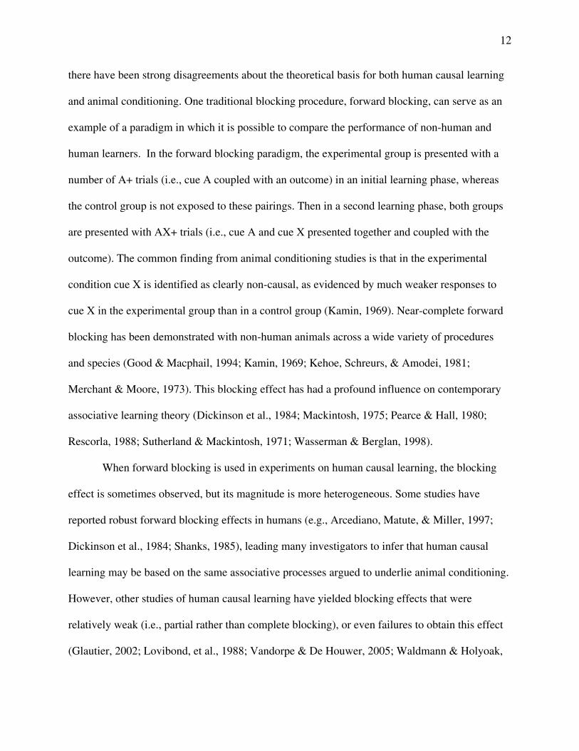
there have been strong disagreements about the theoretical basis for both human causal learning
and animal conditioning. One traditional blocking procedure, forward blocking, can serve as an
example of a paradigm in which it is possible to compare the performance of non-human and
human learners. In the forward blocking paradigm, the experimental group is presented with a
number of A+ trials (i.e., cue A coupled with an outcome) in an initial learning phase, whereas
the control group is not exposed to these pairings. Then in a second learning phase, both groups
are presented with AX+ trials (i.e., cue A and cue X presented together and coupled with the
outcome). The common finding from animal conditioning studies is that in the experimental
condition cue X is identified as clearly non-causal, as evidenced by much weaker responses to
cue X in the experimental group than in a control group (Kamin, 1969). Near-complete forward
blocking has been demonstrated with non-human animals across a wide variety of procedures
and species (Good & Macphail, 1994; Kamin, 1969; Kehoe, Schreurs, & Amodei, 1981;
Merchant & Moore, 1973). This blocking effect has had a profound influence on contemporary
associative learning theory (Dickinson et al., 1984; Mackintosh, 1975; Pearce & Hall, 1980;
Rescorla, 1988; Sutherland & Mackintosh, 1971; Wasserman & Berglan, 1998).
When forward blocking is used in experiments on human causal learning, the blocking
effect is sometimes observed, but its magnitude is more heterogeneous. Some studies have
reported robust forward blocking effects in humans (e.g., Arcediano, Matute, & Miller, 1997;
Dickinson et al., 1984; Shanks, 1985), leading many investigators to infer that human causal
learning may be based on the same associative processes argued to underlie animal conditioning.
However, other studies of human causal learning have yielded blocking effects that were
relatively weak (i.e., partial rather than complete blocking), or even failures to obtain this effect
(Glautier, 2002; Lovibond, et al., 1988; Vandorpe & De Houwer, 2005; Waldmann & Holyoak,

13
1992). In the next subsection we present simulation results to explain the paradoxical findings in
human causal learning.
4.2 Simulation Results
Our simulations are based on two studies of human causal learning, by Vandorpe and De
Houwer (2005; see Table 2) and Wasserman and Berglan (1998; see Table 3). Both studies
report detailed data on the causal ratings as a measure of estimated causal weights for individual
cues. Importantly, the cover stories in these studies made it clear that the causal outcome was a
binary variable, with observers being asked to identify whether foods lead to an allergic reaction
or not. Here we apply our model to these blocking paradigms by comparing predictions based on
two alternative generative functions, linear-sum or noisy-or. Both integration rules have been
used in the literature to account for blocking effects in sequential causal learning (i.e., Rescorla
& Wagner, 1972; Dayan & Kakade, 2000; Carroll, Cheng, & Lu, 2013).
Figure 2 shows the predicted mean weights of each cue as a function of the training trials
in a forward blocking paradigm based on the noisy-or rule and the linear-sum rule. The design by
Vandorpe and De Houwer (2005) includes six A+ trials, followed by six AX+ trials. Human final
causal ratings are indicated by the asterisks in Figure 2. In stage 1 with six A+ trials, simulations
using both the linear-sum rule (right panel in Figure 2) and the noisy-or rule (left panel) capture
the gradual increase of estimated causal strength for cue A as the number of observations
increases. However, after six AX+ trials in stage 2, the models with different integration rules
generate distinct predictions.
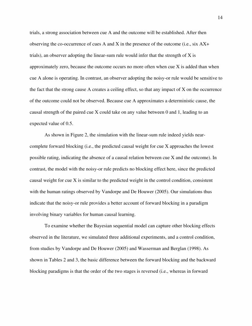
We will first provide an intuitive account for the predictions from the linear-sum and
noisy-or integration rules, and then present the detailed simulation results. After the initial six A+
14
trials, a strong association between cue A and the outcome will be established. After then
observing the co-occurrence of cues A and X in the presence of the outcome (i.e., six AX+
trials), an observer adopting the linear-sum rule would infer that the strength of X is
approximately zero, because the outcome occurs no more often when cue X is added than when
cue A alone is operating. In contrast, an observer adopting the noisy-or rule would be sensitive to
the fact that the strong cause A creates a ceiling effect, so that any impact of X on the occurrence
of the outcome could not be observed. Because cue A approximates a deterministic cause, the
causal strength of the paired cue X could take on any value between 0 and 1, leading to an
expected value of 0.5.
As shown in Figure 2, the simulation with the linear-sum rule indeed yields near-
complete forward blocking (i.e., the predicted causal weight for cue X approaches the lowest
possible rating, indicating the absence of a causal relation between cue X and the outcome). In
contrast, the model with the noisy-or rule predicts no blocking effect here, since the predicted
causal weight for cue X is similar to the predicted weight in the control condition, consistent
with the human ratings observed by Vandorpe and De Houwer (2005). Our simulations thus
indicate that the noisy-or rule provides a better account of forward blocking in a paradigm
involving binary variables for human causal learning.
To examine whether the Bayesian sequential model can capture other blocking effects
observed in the literature, we simulated three additional experiments, and a control condition,
from studies by Vandorpe and De Houwer (2005) and Wasserman and Berglan (1998). As
shown in Tables 2 and 3, the basic difference between the forward blocking and the backward
blocking paradigms is that the order of the two stages is reversed (i.e., whereas in forward
15
blocking A+ trials are followed by AX+ trials, in backward blocking A+ trials precede AX+
trials).
==========================================================
Insert figure 2 here
==========================================================
In human causal learning, an analogous reversal of order occurs in related paradigms
originally developed in the field of animal learning. “Overshadowing” is similar to blocking in
that two cues, A and X, are paired (i.e., AX+), but (unlike the blocking paradigm) neither cue is
ever shown alone paired with a positive outcome. Typically, the two cues overshadow each other
to result in an intermediate level of causal strength for each cue. Two important variants are
“reduced overshadowing” (A- trials followed by AX+ trials), which results in judging cue A as a
weak cause and cue X as a strong cause, i.e., less overshadowing for X; and “recovery from
overshadowing”, which simply reverses the order of presentation so that the A- trials follow the
AX+ trials (i.e., AX+ trials followed by A- trials), resulting in a retroactive reduction in
overshadowing of X.
==========================================================
Insert Table 2 and 3 here
==========================================================

16
As shown in Figure 3 (top), human participants showed substantially different patterns of
causal ratings for the A and X cues for different blocking paradigms. These differences are
captured well by the model based on the noisy-or function (middle), which yields a very high
correlation (.97) and low root-mean-square deviation (RMSE = 0.80) between model predictions
and human performance across all experiments, blocking paradigms and cues. In contrast, the
model results based on the linear-sum rule (bottom in Figure 3) produces a poorer fit, with lower
correlation r = .72, and higher RMSE = 2.41. Our simulation results thus strongly favor the
interpretation that humans typically apply the noisy-or rule in causal sequential learning when
inferring cause-effect relations based on binary outcomes. Hence the simulation results from the
sequential data are consistent with the computational account for summary data from the Power
PC theory, which predicts that when the outcome is a binary variable, the noisy-or rule is
normatively more appropriate than the linear-sum rule for modeling these learning situations
(Cheng, 1997).
4.3 Results and Discussion
As noted earlier, in animal conditioning experiments, the main finding is that rats and
other non-human animals more commonly show a blocking effect in the forward paradigm than
in the backward paradigm (Balleine, Espinet, & Gonzalez, 2005; Denniston, Miller, & Matute,
1996; Miller & Mature, 1996). In contrast, the human causal ratings obtained by Vandorpe and
De Houwer (2005) and Wasserman and Berglan (1998) do not show a difference in blocking
across the two directions for the target cue X (5.0 on a 1-10 rating scale for the forward blocking
paradigm in Vandorpe & De Houwer, 2005; and 4.75 on a 1-9 rating scale for the backward
17
blocking paradigm in Wasserman & Berglan, 2010). In the first study testing backward blocking
in humans, Shanks (1985) noted that the observed magnitude of the blocking effect was
comparable for both forward and backward paradigms (tested within a single experiment). As
shown in Figure 4 (middle), the simulation using the noisy-or rule predicts only a small
difference between the forward and backward paradigms for the target cue X, consistent with the
pattern in the human data, whereas the simulation with the linear-sum rule (bottom) predicts a
considerably stronger blocking effect in the forward than in backward paradigm. Thus while the
prediction based on the noisy-or rule more closely matches the results for these studies of human
causal learning, the prediction based on the linear-sum rule is broadly consistent with findings
from the literature on conditioning with non-human animals.
==========================================================
Insert figure 3 here
==========================================================
Our simulation results thus provide an account of why the forward blocking is less
pronounced in human causal learning than in animal conditioning. It appears that in sequential
causal learning, humans are able to identify whether the outcome variable is binary or continuous
and then select an appropriate causal integration rule depending on the perceived property of
outcome variables. When the outcome variable is binary (i.e., true vs. false, present vs. absent),
humans readily adopt the noisy-or rule (the normative causal integration function for binary
outcome variables; Cheng, 1997; Pearl, 1988). When the outcome variable is perceived as
continuous, humans show a pattern consistent with use of the linear-sum rule.
18
The present simulation results are in agreement with the empirical findings of Mitchell
and Lovibond (2002), who conducted experiments to identify conditions that influence the
magnitude of the forward blocking effect in human causal learning. Their results indicated that
the magnitude of the blocking effect depends on certain characteristics of the outcome variable.
Specifically, these investigators obtained a strong blocking effect when human participants were
instructed that the outcome variable was continuous, so that participants tend to expect that the
net influence of two cues on the magnitude of the effect would be additive. In contrast, when
human observers were instructed that the outcome was a binary variable (i.e., either present or
absent), the blocking effect was much weaker. Our model provides a computational account of
how an abstract property of the outcome variable (continuity versus discreteness) could modulate
the robustness of forward blocking effects for humans.
By contrast, in conditioning paradigms used with rats and other non-human animals, the
outcome may typically be treated as continuous (e.g., reward can vary continuously in magnitude
and/or rate of occurrence; see Gallistel & Gibbon, 2000). Accordingly, non-human animals may
adopt the linear-sum rule as a default model, in essence adding up the causal influences from
individual cues to estimate their net impact on the outcome variable. Our analysis thus clarifies
both the commonalities and differences between human causal learning and animal conditioning.
Recent work has begun to explore transfer to novel cues with animals (Beckers et al., 2006;
Wheeler et al., 2008). Further experimental work should investigate whether non-human animals
have the ability to distinguish outcomes as binary variables (i.e., presence vs. absence of the
footshock) from outcomes as continuous variables (e.g., the duration or strength of the
footshock) ; and if they can, whether animals can flexibly switch to the noisy-or rule for binary
variables when inferring cause-effect relations.
19
5. Simulation of Abstract Transfer Effects in Sequential Causal Learning
5.1 Overview of Empirical Results
The simulations reported in section 4 suggest that humans may be able to select causal
integration rules based on the general characteristics of outcome variables, preferentially using
the noisy-or rule when the outcome variable is perceived as binary, but using the linear-sum rule
when the outcome is perceived as continuous. Yet more remarkably, recent empirical evidence
indicates that humans use more sophisticated selection mechanisms to choose between
alternative learning rules when the nature of the outcome variable is ambiguous. In particular,
researchers find that humans (Beckers, De Houwer, Pineño, & Miller, 2005; Shanks & Darby,
1998) and perhaps rats (Beckers, Miller, De Houwer, & Urushihara, 2006) have the ability to
acquire and transfer abstract causal knowledge in situations where the specific cues are changed
between training and the transfer test. Beckers et al. (2005, 2006; also see Vandorpe, De
Houwer, & Beckers, 2007; Lovibond, Been, Mitchell, Bouton, & Frohardt, 2003; Wheeler,
Beckers, & Miller, 2008) showed that different pre-training conditions using unrelated cues
could prevent or promote the occurrence of forward and backward blocking for target cues. As
an everyday example of this sort of abstract transfer, if a person learns that a cooking
competition in which each contestant prepares several dishes has been won by the chef who
prepared the single best dish (rather than a rival who prepared better dishes on average), this
experience might carryover to create an expectation about how the winner would be determined
in a singing contest. Such abstract transfer effects, in which learning about one set of cause-
effect relations alters the learning of another set of relations based on entirely different stimuli,
pose a serious challenge to all current formal models of sequential causal learning. In the absence
20
of any systematic overlap of features between the cues in different situations, previous models in
sequential causal learning are unable to account for abstract transfer effects. In the next section,
we will present simulation results to explain abstract transfer effects observed in human causal
learning.
To account for these phenomena occurred when the causal cues differ between blocking
training and pre/post-training, we assume that the observed transfer occurs at an abstract level
based on the degree of evidence favoring different causal integration rules. The key idea is that
people can flexibly select the particular integration rule that is most successful in explaining
recent sequentially-presented observations. If new causal cues are then introduced in close
temporal proximity, the causal model that “won” in the initial training phase will also be favored
in interpreting further sequential data. The selected integration rule will then be applied in
subsequent causal inference even with different cues, resulting in abstract transfer of causal
patterns so as to alter the magnitude of blocking effects in the subsequent learning phase.
Within this framework, an explanation can be provided for abstract transfer effects,
which show that causal inference depends strongly on its temporal context (i.e., information
provided shortly before or after some critical event). Suppose that a subject is exposed to pre-
training data before observing new data. The subject evaluates the evidence to find the best
causal generative model with a specific integration rule to explain the observations. The subject
then proceeds to use the selected causal integration rule to make subsequent inferences with new
data without evaluating the other causal rules, as long as the subsequent experimental trials do
not evoke any strong bias to alternative causal models. The subject thus uses the procedure of
model selection to enable knowledge transfer from the pre-training data to help interpret
subsequent observations in a new context,
21
This computational framework can be readily extended to account for a related type of
abstract causal transfer, produced by post-training (Beckers et. al, 2005). In this scenario,
learners first observe the occurrence of cues and outcomes for one set of data. The contingencies
are such that this data can be equally well explained by the linear-sum and noisy-max rules,
making it impossible to confidently select one of the two alternative models. To cope with this
situation, we hypothesize that the learner (at least for a human—post-training effects have not
been tested with other animals) will often maintain both models. Although maintaining two
alternative models would presumably impose an extra burden on working memory, there is
evidence from other reasoning paradigms that adult humans are capable of keeping two models
in mind (e.g., Johnson-Laird, 2001). Learners are then exposed to post-training data with
different cues, for which the contingencies unambiguously favor one of the two alternative
integration rules. Our model postulates that the unambiguous post-training can be used to
(retroactively) weight the causal estimates from two models for the initial data set (which used
different cues), so that the model favored for the post-training data comes to retroactively
dominate (but not eliminate) its rival as an explanation of the initial data. This type of post-
training effect, which can be modeled by model averaging (Courville, Daw, Gordon, &
Touretzky, 2003), is an example of what is often termed “retroactive reevaluation” of causal
strength.
5.2 Simulation Results
In this section, we report simulation results for two cases: (1) experiments that used a pre-
training design to show abstract transfer effects (Experiments 2 and 3 in Beckers et al., 2005),
and (2) experiments using a post-training design that demonstrate retrospective reevaluation
(Experiment 4 in Beckers et al., 2005). Because the outcome variables in these studies were

22
continuous (degrees of allergic reaction), the model simulations are based on the comparisons
between two causal integration rules, linear-sum and noisy-max.
Transfer Effects with Pre-training
Table 4 outlines an experimental design in which humans were given different types of
pre-training in Phase 1, followed by sessions of forward blocking (Experiment 2 in Beckers et
al., 2005) or backward blocking (Experiment 3 in Beckers et al., 2005). For the additive
conditions, Phase 1 consisted of trials in which individual food cues, G or H, were paired with a
moderate allergic reaction (indicated by +), and the combination GH was paired with a strong
allergic reaction (indicated by ++). This occurred prior to the blocking session in Phases 2 and 3,
in which different food cues, A and AX, were paired with a moderate allergic reaction (indicated
by +). The subadditive conditions provided Phase 1 trials in which food cues G, H and the
combination GH were each paired with a moderate allergic reaction (indicated by +). The
blocking sessions (Phase 2 and 3) were identical for both additive and subadditive conditions. If
we removed the pre-training, the paradigms would be standard forward and backward blocking
designs of the sort to which we have applied our model (see Section 4). A critical design feature
was that completely different cues were used in the pre-training Phase 1 (cues G, H) and in
Phases 2 and 3 (cues A, X). If there was no abstract transfer, we would expect standard forward
and backward blocking effects for the target X, regardless of which pre-training conditions were
included. Control cues K and L were only presented in KL+ trials during Phase 3.
After completing these three phases, participants were asked to rate how likely each food
cue separately would cause an allergic reaction. Human results (see Figure 5, left columns)
showed that the target cue X was blocked after additive pre-training but not after subadditive
pre-training. More precisely, additive pre-training resulted in a lower human rating for the target

23
cue X than for the control cues, K and L, indicating a strong blocking effect. By contrast, after
subadditive pre-training there was little difference between the ratings for X, K and L, indicating
the absence of a blocking effect.
==========================================================
Insert Table 4 here
==========================================================
Our computational theory was tested by using the data in the pre-training phase (i.e.,
phase 1) to run the sequential models with the linear-sum and noisy-max integration rules, and
then using model selection to determine which causal model was more likely for the two
experimental conditions (additive versus subadditive pre-training). As shown in Figure 4, the
first two stages (8G+ and 8H+) did not distinguish between causal models adopting different
integration rules, noisy-max and linear-sum, with the log ratio of model evidence being close to
0. However, after the third stage of the pre-training trials (8GH++ in the additive condition and
8GH+ in the subadditive condition), the log ratio of model evidence clearly revealed greater
support for the noisy-max model (i.e., greater than 0) in the additive condition, and for the linear-
sum model for the subadditive condition (indicated by a negative value of the log ratio).
==========================================================
Insert figure 4 here
==========================================================

24
We then applied the selected models to the training data in Phases 2 and 3 to update the
distributions of causal weights for individual cues. To compare with human ratings, we
computed the mean weight for each cue with respect to the posterior distribution. The right
panels in Figure 5 show that the mean weights, calculated using the selected causal model, are in
good agreement with human causal ratings. The linear-sum model generates accurate predictions
for the additive group: the mean weight for the target cue X is much lower than weights for the
control cues K and L, indicating blocking of causal learning for cue X. In contrast, the noisy-max
model gives accurate predictions for the subadditive group: the mean weight for cue X is slighter
lower than the weights for the control cues K and L, consistent with a much weaker blocking
effect for cue X in the subadditive group.
==========================================================
Insert figure 5 here
==========================================================
Transfer Effects with Post-training
We also applied our model to explain the impact of post-training on human causal
judgments. Experiment 4 reported by Beckers et al. (2005) showed that post-training (i.e.,
training with additional new stimuli after the target cues) is able to alter human judgments about
previously-acquired cause-effect relations. As shown in Table 5, Phases 1 and 2 now correspond
to a forward blocking training session, with cues A+ and AX+, whereas Phase 3 is a post-
training phase with different cues (i.e., cue G and H) paired with severe or moderate outcomes
(corresponding to additive and subadditive conditions, respectively). After the post-training
phase, human participants were asked to evaluate the causal strength for individual cues (i.e., A

25
and X). In other words, the design in the post-training study is the same as for the pre-training
study described earlier, but with a different order of training phases. The experimental results
(Beckers et al., 2005) show that post-training (either additive or subadditive) impacts human
causal ratings for cues, despite being presented after the blocking training phases. The impact of
post-training is weaker than that of pre-training, but nevertheless significant as shown in Figure 6
(left).
From a computational perspective, post-training differs from pre-training in that post-
training precludes model selection prior to the blocking session, because the data for the initial
training is inherently ambiguous between two rival integration rules (i.e., after observing
8A+/8AX+ trials, the model evidence is equal for the linear-sum and the noise-max models,
making it impossible to select the single best model). It is plausible that the subject therefore
maintain two competing models (linear-sum and noisy-max) as possible explanations of the data.
However, after receiving the unambiguous post-training data with different cues, the learner
reassesses the estimates for the initial data, by taking into consideration of how well the
alternative models could explain the post-training data in Phase 3. In our simulations, the mean
causal strengths based on each model were estimated using observations in the first two training
phases, and the final strengths are calculated by averaging the two estimates weighted by the
probability of supports for each model.
==========================================================
Insert Table 5 here
==========================================================

26
==========================================================
Insert figure 6 here
==========================================================
As shown in Figure 6, human ratings for the critical cue (X) depend on whether
participants viewed the additive or subadditive conditions during the post-training phase (though
the magnitude of this abstract transfer effect was reduced relative to that obtained in the
comparable experiment using pre-training). The comparisons to human data in Figure 6 show
that model averaging qualitatively captures the impact of post-training, as exposure to additive
post-training yielded lower ratings for cue X than did exposure to subadditive post-training.
The experiments by Beckers et al. (2005) provide clear evidence of abstract transfer. The
pre-training phase provided sufficient evidence to favor one model over the other, whereas such
information was not available in the post-training design. Model selection, in which a subject
first selects the model with the highest evidence support, and then makes inferences based on the
parameters/functions of the selected model, involves less computation than does model
averaging. However, model selection requires clear evidence favoring one “best” model over the
alternatives. By contrast, model averaging requires more computation (imposing additional
working memory load), as it involves making inferences using multiple candidate models. We
expect that under speed pressure, or with manipulations that increase working memory load,
early selection of a single model will be preferred. This selected model will then become the
default unless later observations provide contradictory evidence. Hence, the choice between
model selection and model averaging is likely to depend on both the strength of the evidence
27
favoring the “best” model (with stronger evidence favoring model selection), and on the
availability of memory and processing resources to track multiple models (with greater resources
favoring model averaging).
6. Simulation of Primacy Effect in Sequential Causal Learning
6.1 Overview of Empirical Results
It has long been known that the presentation order of stimuli can affect causal judgments
when observing data that are presented sequentially. However, two opposing types of ordering
effects have been observed. Some studies have reported a recency effect, in which final causal
beliefs are biased towards the information that is presented later (López, Shanks, Almaraz, &
Fernández, 1998; Collins & Shanks, 2002). Other studies have shown an opposite primacy
effect, in which early presented information plays a more important role in determining the final
causal judgments (Dennis & Ahn, 2001; Danks & Schwartz, 2006). For example, Dennis and
Ahn (2001) first showed participants a sequence of 20 trials demonstrating a generative causal
relationship between contact with a plant (a candidate cause) and an allergic reaction (effect)
(with p(allergy|plant) = 0.9 and p(allergy|no plant) = 0.1, consistent with causal power of 0.89),
followed by a sequence of 20 trials demonstrating a preventive causal relationship (with
p(allergy|plant) = 0.1 and p(allergy|no plant) = 0.9, consistent with a preventive causal power of
0.89). We will refer to this as the “+/-” condition (i.e., trials consistent with symmetrical
generative and then preventive power). The other half of participants were assigned to a -/+
condition with the reversed sequence order (i.e., trials indicating a preventive cause followed by
trials indicating a generative cause). Dennis and Ahn found that final ratings of the causal
28
relation between the plant and allergy was greater when the generative cause was presented first
(+/- condition) than when preventive cause was (-/+ condition) (see Figure 7).
The recency effects observed in the above studies have been interpreted as providing
empirical evidence supporting sequential models based on prediction errors that involve
“tracking” the recent data in the sequence (i.e., the Rescorla-Wagner model). In contrast,
observations of primacy effects have been taken as evidence supporting the construction of an
explicit mental model (Dennis & Ahn, 2001). This model is formed using information received
at the beginning of a sequence; later information is discounted if it contradicts the prediction of
the established mental model. However, as Danks and Schwartz (2006) have pointed out, a
theory based on minimizing prediction errors can potentially exhibit primacy effects if the
learning rate, i.e., how fast a subject can learn the causal relationship and is related to in our
model (see more details in Appendix), is assumed to vary over time. In fact, our sequential
Bayesian model assumes for independent reasons (see below) that the learning rate varies. In the
following subsection we elaborate on this aspect of the model, presenting simulation results
showing a primacy effect in some experimental conditions.
6.2 Simulation Results
Because the experiment reported by Dennis and Ahn (2001) clearly used an outcome that
was a binary variable (the allergic reaction was either present or absent), we applied the noisy-or
integration rule for generative causes and the corresponding noisy-and-not rule for preventive
causes (Cheng, 1997; Yuille & Lu, 2006). As in previous simulations of causal learning
(Griffiths & Tenenbaum, 2005; Lu et al., 2008), a background cause with positive causal power
was included to generate an effect, so that a preventive cause can show its influence. The causal
29
weight of the background cause was assigned an initial uninformative prior following a uniform
distribution between 0 and 1. Because the cue (e.g., a plant in Dennis and Ahn’s study) can be
generative or preventive, the causal weight of the cue was constrained to the range of [-1,1],
where the sign indicates the causal direction, and the absolute value of the causal weight
corresponds to a probability, bounded within 0 and 1. The model using the noisy-or rule
presented in Section 4 assumes that the learning rate, corresponding to , varies depending on
the value of the estimated causal weight. The varying learning rate parameter also helps keep the
sampled weight values within the theoretically-determined bounds, because the absolute values
of the weights represent the probabilities. Specifically, when the causal weight is estimated to
have a mean with absolute value of 0.5, for which the uncertainty is largest (due to the binomial
distribution) in determining the occurrence of the effect, then the model applies the maximum
learning rate; in contrast, as the estimated weight approaches a limit (i.e., the ceiling at absolute
value 1 or the floor at 0), the learning rate is reduced by a scaling factor. This scaling factor is
calculated using a non-normalized Gaussian function by comparing the estimated causal weight
with a mean of 0.5 and standard deviation of 0.1. Hence, the scaling factor follows a bell-curved
shape so that the learning rate is maximal when the causal weight is 0.5, and minimal when the
causal weight is 0, 1 (generative) or -1 (preventive). Such variation in learning rate slows down
the change in causal weight over trials when the estimate is close to the ceiling (i.e., causal
power is close to 1 or -1).
Figure 7 shows the human causal ratings and simulation results for Experiment 1
reported by Dennis and Ahn. The simulation results qualitatively account for the observed
primacy effect in human causal judgments (i.e., the final causal judgment was positive when the
generative causal sequence was presented first in the +/- experimental condition, but negative
30
when the preventive causal sequence was presented first in the -/+ experimental condition).
Nonetheless, there are differences between the pattern of human ratings and the model
predictions. In particular, an asymmetry is apparent in the human ratings, which show a stronger
primacy effect when the sequence with generative power was presented first than when the
preventive power was encountered first. Dennis and Ahn (2001) suggested that this asymmetry
may be due to an inherent bias favoring generative over preventive cause. Our sequential causal
model does not incorporate any preference for a particular causal direction, and hence does not
account for the observed asymmetry.
==========================================================
Insert figure 7 here
==========================================================
In a second study showing primacy effects, Danks and Schwartz (2006) used a similar
design to investigate whether the primacy effect depends on the magnitude of causal power. In
conditions with strong causal strength, the presence of the cause (a plant) and the effect (a rash)
were arranged to yield a causal power of 0.89 (i.e., P(rash|plant) = 0.9, P(rash|no plant) = 0.1); in
the conditions with weak causal strength, the causal power was 0.57 (e.g., P(rash|plant) = 0.7,
P(rash|no plant) = 0.3); and the causal power was set to 0.5 in the unbiased condition. As shown
in the left plot of Figure 8, midpoint ratings (write bars in Figure 8) after observing 20 trials were
presented to show the learning in the first half of the sequence, and final ratings (grey bars) after
observing all 40 trials were used to illustrate the presence of primacy effects. Significant primacy
effects were found in the strong +/- and weak -/+ conditions, in that final ratings were
significantly different from zero and biased toward the causal direction presented in the first half
31
of the sequence (see Figure 8, left). Model simulations also yield primacy effects in the two
strong conditions, strong +/- and strong-/+. However, when the causal power is reduced, the
model does not reveal a primacy effect in either of the weak conditions. Thus, the model’s
performance is highly dependent on values of causal power, and the model is more sensitive to
this manipulation than are human observers.
Although our sequential Bayesian model can yield a primacy effect under certain
conditions, the simulation results need to be interpreted in caution. One determinant in the
present sequential causal model is prediction errors, which tend to induce a recency effect (as is
the case for the Rescorla-Wagner model). However, the varying learning rate can instead yield a
primacy effect under certain conditions. We suspect that at least two learning strategies are
involved in primacy effects. (1) Observers may use early evidence to anchor a causal hypothesis.
The observer then accepts later evidence if it confirms the anchor hypothesis, but discounts the
evidence if it is inconsistent with the anchor hypothesis. (2) Standard sequential causal learning
based on the correction of prediction errors but allowing the learning rate change over time can
also yield a primacy effect. Our simulation results confirm the possibility of the second strategy,
but do not reject the first. An analysis of individual differences reported by Danks and Schwartz
(2006) suggests that these two strategies co-exist in human causal learning with sequential data.
In addition, the primacy effect observed in our simulation results is sensitive to the learning rate
parameter, suggesting an important factor that may contribute to individual differences. If
different observers use different learning rates, some would exhibit a primacy effect, but others
may show a recency effect.
32
==========================================================
Insert figure 8 here
==========================================================
7. General Discussion
In the present paper we have presented a new model of sequential causal learning,
implemented using particle filters. Our model is the first to combine computational mechanisms
of rule transfer with sequential weight updating, and the first to explicitly compare performance
under three major integration rules (linear-sum, noisy-or and noisy-max) in sequential causal
learning. The model incorporates key ideas exploited in previous work (alternative integration
rules, Bayesian sequential updating of strength distributions, model selection and model
averaging), showing that these can work together to explain a broad range of phenomena. The
phenomena the model can account for include (1) order effects in causal sequential learning, as
exemplified by the difference in performance associated with various blocking paradigms; (2)
evidence that patterns of human causal learning are influenced by their understanding of the
nature of the outcome variable (in particular, whether it takes on binary or continuous values);
(3) evidence that in addition to learning about specific causal cues, humans are able to transfer
their acquired knowledge to guide causal learning with entirely different cues; (4) evidence that
in some sequential-learning situations, final causal judgments can show a primacy effect, being
influenced more by information presented early in the sequence.
The key assumption of our computational model is that learners have available multiple
causal generative models, each reflecting a different integration rule for combining the influence

33
of multiple causes (Waldmann, 2007; Lucas & Griffiths, 2010). The evidence that people are
able to use multiple integration rules implies that an adequate model of sequential causal learning
must be more flexible than models based solely on the linear-sum rule used in most existing
models (the Rescorla-Wagner model, and the Bayesian model developed by Dayan and his
colleagues). As the present theory demonstrates, sequential models can be based on alternative
integration rules while maintaining the basic idea that learning is guided by prediction errors.
Yuille (2005, 2006) has demonstrated mathematically that linear and non-linear variants of
sequential learning models can perform maximum likelihood estimation for a range of different
integration rules, and has shown formally how Bayesian models at the computational level can
be related to algorithmic models of sequential causal learning.
Kruschke (2008) developed a sequential model using the noisy-or rule, and compared its
performance in several blocking paradigms with that of a model based on a Kalman-filter
implementation of the linear-sum rule. This sequential model employed Bayes’ rule to update the
distribution of beliefs on causal weights on each trial by combining the estimates of causal
weights learned from previous trials with the data observed in the current trial. However,
Kruschke’s model does not incorporate model selection to choose among alternative integration
rules, and hence provides no basis for explaining abstract causal transfer. In addition, the model
implemented by Kruschke disenabled the dynamic prediction module in the Kalman-filter
implementation, which allows uncertainty of learned causal weights to increase with the passage
of time. Given that forgetting is an essential component of a psychological model of causal
learning, the absence of an account of forgetting is a serious theoretical limitation. To overcome
this limitation, we designed updating procedures implemented as particle filters. By applying
34
iterative prediction and correction steps, the parameters of the model can be updated as new data
arrives using prediction errors, for any causal integration rule.
The building blocks for our computational theory of sequential causal learning are
standard Bayesian procedures that have been used previously in theories of causal reasoning and
animal conditioning: parameter estimation, model selection, and model averaging. For example,
Cheng's (1997) power PC theory uses parameter estimation of the weights of a noisy-or
generative model to account for human performance in causal learning tasks. Similarly, Daw et
al. (2008) estimated the parameters of a linear-sum model to predict the performance of rats in
conditioning experiments. Model selection has been proposed to account for human performance
when deciding whether a cue should or should not be accepted as causal (Griffiths &
Tenenbaum, 2005; also see Carroll, Cheng, & Lu, 2013). Lucas and Griffiths (2010) developed a
hierarchical model to explain how abstract causal knowledge of the form of causal relations can
influence human causal judgments, an approach that is quite consistent with our emphasis on
selection among alternative integration rules. Model averaging has also been used to account for
phenomena related to causal learning. For example, Courville et al. (2003) used model averaging
to explain how animals cope with uncertainties about contingencies in two conditioning
paradigms (second-order conditioning and conditioned inhibition).
Although the building blocks of the present model have been explored in the literature, to
our knowledge the present theory is the first to integrate these core theoretical elements within a
unified computational framework in order to explain a broad range of phenomena that arise in
human sequential causal learning. This model provides an explanation of why patterns of human
causal learning are similar to yet different from those observed in studies of conditioning with
non-human animals. In particular, humans readily adopt a noisy-or integration rule when
35
learning about binary-valued outcomes, a rule that yields little difference between forward and
backward blocking (Shanks, 1985; Vandorpe & De Houwer, 2005; Wasserman & Berglan,
2010). In contrast, animals in conditioning paradigms appear to adopt a linear-sum rule, which
yields stronger forward blocking with much weaker backward blocking (Balleine et al., 2005;
Denniston et al., 1996; Miller & Mature, 1996).
Most notably, the theory accounts for abstract transfer effects, observed when different
pre-training alters subsequent learning with completely different stimuli (Beckers et al., 2005).
Using the standard approach of Bayesian model selection, the learner selects the model that best
explains the pre-training data. Then, during subsequent learning with different cues, the learner
employs the favored model to estimate causal weights. Because the information provided in the
transfer phase is identical for all experimental conditions, only pre-training with different cues
can account for the differences observed on the transfer test. By assuming that humans are also
able to perform model averaging when data are ambiguous between two alternative integration
rules, our theory also can explain the distinct pattern of transfer produced by post-training
(Beckers et al., 2005), in which later training with different cues alters responses to cause-effect
relations learned earlier. No previous model of sequential learning can account for abstract
causal transfer, because all previous models are restricted to learning causal weights for specific
causal cues. In the absence of any systematic featural overlap between the cues in different
situations, such models provide no basis for transfer effects.
Abstract transfer effects of this sort may reflect the fact that causal influences in the
environment typically are stable over a long timescale, so that the causal functions underlying
observations that occur close in time are expected to be similar, even if the specific cues vary.
As a consequence, a causal system will benefit from the ability to implicitly or explicitly learn
36
abstract knowledge of the environment over a temporal interval, coupled with the ability to
transfer this acquired knowledge to guide causal inferences about different cues that occur close
to, but outside of, the initial time period. Ahn and her colleagues (Luhmann & Ahn, 2011; Taylor
& Ahn, 2012) have provided evidence supporting this view, showing that humans develop
expectations during causal learning, and that these expectations affect the interpretations of the
causal beliefs derived from subsequently-encountered covariation information.
Although the present theory postulates a powerful mechanism for learning cause-effect
relations, it certainly does not require the full power of relational reasoning (Holyoak, 2012).
Abstract transfer of causal patterns to different cues can be explained by probabilistic models, as
demonstrated in recent work on causal reasoning and analogy (Holyoak, Lee, & Lu, 2010) and
on learning sequence sets with varied statistical complexity and transformational complexity
(Gureckis & Love, 2010). However, the statistical learning mechanisms incorporated into the
present theory go well beyond any traditional associative account of sequential learning in
postulating multiple integration rules available to the learner, and in providing an explicit model
of the learner's uncertainty.
Our theory nonetheless exploits prediction error to guide the sequential updating process,
thus preserving what seems to be the most basic contribution of the Rescorla-Wagner model. As
a result, the present model enables us to account for trial order effects that occur in blocking
experiments, which cannot be accounted for by models that only deal with summarized data
(Cheng, 1997; Griffiths & Tenenbaum, 2005; Lu et al., 2008a). However, the present theory is
considerably more powerful than previous accounts of sequential causal learning. The Rescorla-
Wagner model (Rescorla & Wagner, 1972) and its many variants (see Shanks, 2004) only update
point estimates of causal strength, and thus are unable to represent degrees of uncertainty about

37
causal strength (Cheng & Holyoak, 1995). Similar limitations hold for a previous model of
sequential learning based on the noisy-or integration function (Danks et al., 2003). By adopting a
Bayesian approach, we have provided a formal account of how a learner's confidence in the
causal strength of a cue can change over the course of learning, for any well-specified integration
rule. The present theory goes beyond previous accounts of dynamical causal learning (Dayan &
Kakade, 2000; Daw al., 2008) with respect to its core assumption that learners (human and
perhaps non-human as well) are able to choose among multiple generative models that might
explain observed data. The theory thus captures what may be a general adaptive mechanism by
which biological systems learn about the causal structure of the world. The theory might be
extended, perhaps using techniques developed by Kemp and Tenenbaum (2008), to allow for
new models to be developed when existing models fail to adequately fit the data. Such a
generalized theory would allow abstract knowledge of causal models evolve and develop over
time. To test such a theory, psychological experiments should manipulate the causal information
presented during the pre-training phase. In addition, the present theory of sequential causal
learning may potentially be integrated with models of how non-causal relations can be acquired
from examples (Lu, Chen, & Holyoak, 2012).
38
Footnotes
1 As Danks, Griffiths and Tenenbaum (2003) observed, any model of causal learning from
summary data can be applied to sequential learning simply by keeping a running tally of the four
cells of the contingency table (defined by the presence versus absence of a causal cue and the
effect), applying the model after accumulating n observations, and repeating as n increases. This
approach suffices to model the standard negatively-accelerating acquisition function observed in
studies of sequential learning. However, such a “pseudo-sequential” model cannot explain order
effects in learning (as all the data acquired so far are used at each update and weighted equally).
Moreover, a plausible psychological model will need to operate within realistic capacity limits. It
seems unlikely that humans can store near-veridical representations of all the specific occasions
on which possible causes are paired with the presence or absence of effects. Rather, a realistic
sequential model will likely involve some form of on-line extraction of causal relations from
observations of covariations among cues.
Acknowledgements
This research was supported by NSF grant BCS-0843880 to HL, FWO grant G.0766.11 to TB,
and AFOSR grant FA 9550-08 1-0489 to AY. A preliminary report of an earlier version of the
model was presented at the Thirtieth Annual Conference of the Cognitive Science Society
(Washington, D. C., July 2008). We thank Keith Holyoak, Michael Lee, and two anonymous
reviewers for helpful comments on earlier drafts. We thank David Danks for sharing the detailed
design of empirical studies from his lab, and Michael Lee and two anonymous reviewers for their
insightful suggestions. Correspondence may be directed to Hongjing Lu ([email protected]).
MATLAB code for the simulations reported here is available from the first author.
39
Appendix
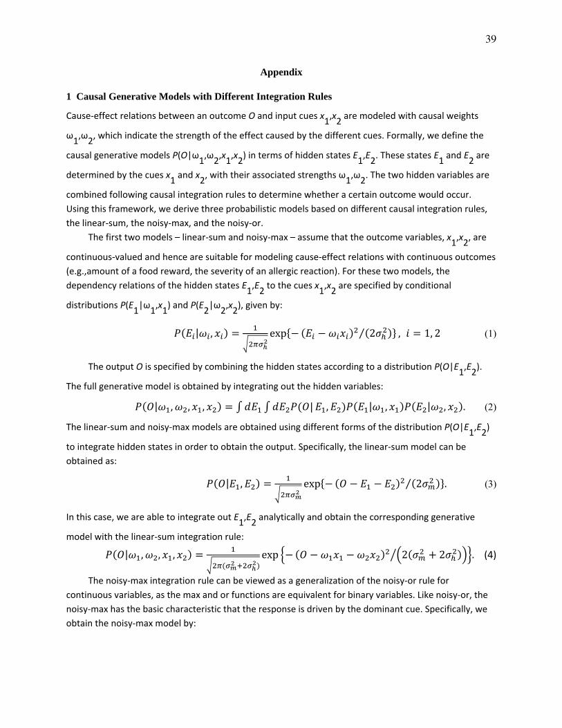
1 Causal Generative Models with Different Integration Rules
Cause‐effect relations between an outcome O and input cues x1,x2 are modeled with causal weights
ω1,ω2, which indicate the strength of the effect caused by the different cues. Formally, we define the
causal generative models P(O|ω1,ω2,x1,x2) in terms of hidden states E
1,E2. These states E
1 and E
2 are
determined by the cues x1 and x
2, with their associated strengths ω
1,ω2. The two hidden variables are
combined following causal integration rules to determine whether a certain outcome would occur.
Using this framework, we derive three probabilistic models based on different causal integration rules,
the linear‐sum, the noisy‐max, and the noisy‐or.
The first two models – linear‐sum and noisy‐max – assume that the outcome variables, x1,x2, are
continuous‐valued and hence are suitable for modeling cause‐effect relations with continuous outcomes
(e.g.,amount of a food reward, the severity of an allergic reaction). For these two models, the
dependency relations of the hidden states E1,E2 to the cues x
1,x2 are specified by conditional
distributions P(E1|ω
1,x1) and P(E
2|ω
2,x2), given by:
| , exp 2⁄ , 1, 2 (1)
The output O is specified by combining the hidden states according to a distribution P(O|E1,E2).
The full generative model is obtained by integrating out the hidden variables:
| , , , | , | , | , . (2)
The linear‐sum and noisy‐max models are obtained using different forms of the distribution P(O|E1,E2)
to integrate hidden states in order to obtain the output. Specifically, the linear‐sum model can be
obtained as:
| , exp 2⁄ . (3)
In this case, we are able to integrate out E1,E2 analytically and obtain the corresponding generative
model with the linear‐sum integration rule:
| , , , exp 2 2 . (4)
The noisy‐max integration rule can be viewed as a generalization of the noisy‐or rule for
continuous variables, as the max and or functions are equivalent for binary variables. Like noisy‐or, the
noisy‐max has the basic characteristic that the response is driven by the dominant cue. Specifically, we
obtain the noisy‐max model by:
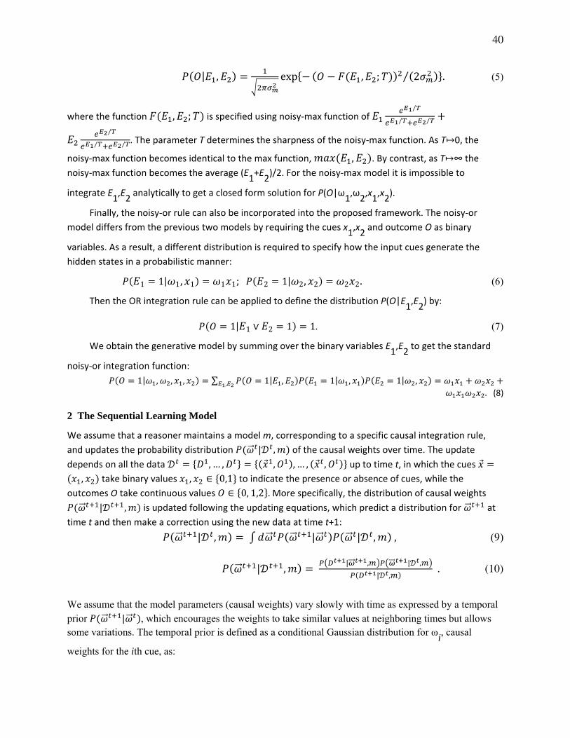
40
| , exp , ; 2⁄ . (5)
where the function , ; is specified using noisy‐max function of ⁄
⁄ ⁄
⁄
⁄ ⁄ . The parameter T determines the sharpness of the noisy‐max function. As T↦0, the
noisy‐max function becomes identical to the max function, , . By contrast, as T↦∞ the
noisy‐max function becomes the average (E1+E2)/2. For the noisy‐max model it is impossible to
integrate E1,E2 analytically to get a closed form solution for P(O|ω
1,ω2,x1,x2).
Finally, the noisy‐or rule can also be incorporated into the proposed framework. The noisy‐or
model differs from the previous two models by requiring the cues x1,x2 and outcome O as binary
variables. As a result, a different distribution is required to specify how the input cues generate the
hidden states in a probabilistic manner:
1 1| 1, 1 1 1; 2 1| 2, 2 2 2. (6)
Then the OR integration rule can be applied to define the distribution P(O|E1,E2) by:
1| 1 ∨ 2 1 1.(7)
We obtain the generative model by summing over the binary variables E1,E2 to get the standard
noisy‐or integration function:
1| , , , ∑ 1| , 1| , 1| ,,
. (8)
2 The Sequential Learning Model
We assume that a reasoner maintains a model m, corresponding to a specific causal integration rule,
and updates the probability distribution | , of the causal weights over time. The update
depends on all the data , … , , , … , , up to time t, in which the cues
, take binary values , ∈ 0,1 to indicate the presence or absence of cues, while the outcomes O take continuous values ∈ 0, 1,2 . More specifically, the distribution of causal weights
| , is updated following the updating equations, which predict a distribution for at
time t and then make a correction using the new data at time t+1:
| , | | , , (9)
| , | , | ,
| ,. (10)
We assume that the model parameters (causal weights) vary slowly with time as expressed by a temporal prior | , which encourages the weights to take similar values at neighboring times but allows some variations. The temporal prior is defined as a conditional Gaussian distribution for ωi, causal
weights for the ith cue, as:

41
1
2 2exp
22 2 , 1, 2. (11)
This prior allows the weights to vary from trial to trial. The amount of variation is controlled by the
parameter . In the limit as → 0, weights become fixed and do not change. For larger values of
the weights can change significantly from one trial to the next. Similar priors have been used in models
of animal conditioning (Daw, et al., 2007). The use of a temporal prior ensures that the model is
sequential and is sensitive to the order of the time sequences of cue‐outcome pairs.
The sequential Bayesian model is optimal, in the sense that it gives the conditional distribution of
the weights conditioned on all the data. With the dynamic component, it updates this distribution
recursively from | , (i.e., without needing to store all the previous cue‐outcome pairs).
Note that if the probability distributions | and | , are Gaussian, then the
sequential Bayesian model simplifies to updating the parameters of Gaussian distributions, which can be
done using algebraic equations (Ho & Lee, 1964), corresponding to the standard Kalman filter as used in
previous models (Dayan et al., 2000).
We can contrast the sequential Bayesian with the Rescorla‐Wagner algorithm (Rescorla & Wagner,
1972), which is a standard procedure for estimating weight parameters for sequential data (e.g., in
animal conditioning experiments). Formally, weights are updated as new data arrive by
, , , where , , depends on the difference between the new outcome
and the prediction. The sequential Bayesian model becomes very similar to Rescorla‐Wagner for
specific choices of the probability distributions. A necessary, but not sufficient condition, is that the
distributions become strongly peaked so that uncertainty is removed and the Bayesian model merely
has to track the mean state.
Though the sequential Bayesian model has some similarity to the Rescorla‐Wagner model (e.g.,
modifying weights based on prediction error), it differs in several aspects. First, the Rescorla‐Wagner
model corresponds to a specific causal integration rule, linear‐sum, for representing cause‐effect
relations. Second, it updates the weights/parameters without taking uncertainty into account, and
therefore does not model the probability of observing the data, as is required to perform model
selection. Third, there is no theoretical framework that allows Rescorla‐Wagner to do model selection.
Fourth, there is no natural way to degrade the Rescorla‐Wagner algorithm to test robustness or allow
for limited neural resources. Although the Rescorla‐Wagner model has had considerable success dealing
with many complex phenomena, such as some forms of blocking, it is unable to account for the complex
phenomena we deal with in the present paper.
3 Theory of Causal Transfer
Our theory assumes that a reasoner has a set of different generative models for learning cause‐effect
relations and is able to choose between them based on observations, and then apply the selected
models to further sequential data. As specified in section 1, each generative model m is specified by a
probability distribution P(D| ω,m) for generating the data D (i.e., the trial sequences of cue‐outcome
events) in terms of parameters ω (e.g., measures of causal strength). Combined with the sequential
Bayesian framework, we can assess three quantities. (1) We can estimate the probability distribution of
the weights given the data | ,,
, and estimate properties such as the mean
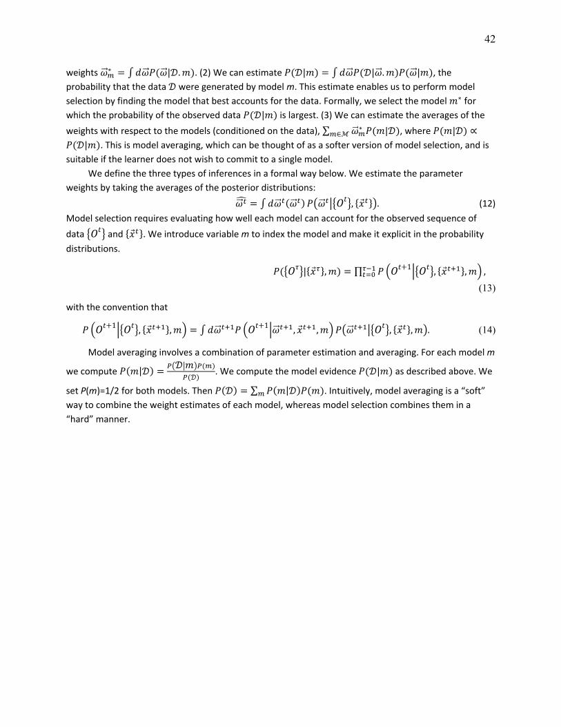
42
weights ∗ | . . (2) We can estimate | | . | , the
probability that the data were generated by model m. This estimate enables us to perform model
selection by finding the model that best accounts for the data. Formally, we select the model ∗ for
which the probability of the observed data | is largest. (3) We can estimate the averages of the
weights with respect to the models (conditioned on the data), ∑ ∗ |∈ , where | ∝| . This is model averaging, which can be thought of as a softer version of model selection, and is
suitable if the learner does not wish to commit to a single model.
We define the three types of inferences in a formal way below. We estimate the parameter
weights by taking the averages of the posterior distributions:
, . (12) Model selection requires evaluating how well each model can account for the observed sequence of
data and . We introduce variable m to index the model and make it explicit in the probability
distributions.
| , ∏ 1 , , ,
(13)
with the convention that
1 , , 1 , , , , . (14)
Model averaging involves a combination of parameter estimation and averaging. For each model m
we compute | . We compute the model evidence | as described above. We
set P(m)=1/2 for both models. Then ∑ | . Intuitively, model averaging is a “soft”
way to combine the weight estimates of each model, whereas model selection combines them in a
“hard” manner.
43
References
Anderson, B. D. O., & Moore, J. B. (1979). Optimal filtering. Englewood Clifss, NJ: Prentice-
Hall.
Arcediano, F., Matute, H., & Miller, R. R. (1997). Blocking of Pavlovian conditioning in
humans. Learning and Motivation, 28(2), 188-199.
Balleine, B. W., Espinet, A., & Gonzalez, F. (2005). Perceptual learning enhances retrospective
revaluation of conditioned flavor preferences in rats. Journal of Experimental Psychology:
Animal Behavior Processes, 31, 341-350.
Beckers, T., De Houwer, J., Pineño, O., & Miller, R. R. (2005). Outcome additivity and outcome
maximality influence cue competition in human causal learning. Journal of Experimental
Psychology: Learning, Memory and Cognition, 31, 238-249.
Beckers, T., Miller, R. R., De Houwer, J., & Urushihara, K. (2006). Reasoning rats: Forward
blocking in Pavlovian animal conditioning is sensitive to constraints of causal inference.
Journal of Experimental Psychology: General, 135(1), 92-102.
Brown, S. D., & Steyvers, M. (2009). Detecting and predicting changes. Cognitive Psychology,
58(1), 49-67.
Buehner, M. J., Cheng, P. W., & Clifford, D. (2003). From covariation to causation: A test of the
assumption of causal power. Journal of Experimental Psychology: Learning, Memory, and
Cognition, 29, 1119-1140.
Burgi, P., Yuille, A. L., & Grzywacz, N. M. (2000). Probabilistic motion estimation based on
temporal coherence. Neural Computation, 12(8), 1839-1867.
44
Carroll, C. D., Cheng, P. W., & Lu, H. (2013). Inferential dependencies in causal inference: A
comparison of belief-distribution and associative approaches. Journal of Experimental
Psychology: General, 142(3), 845-863.
Cheng, P. W. (1997). From covariation to causation: A causal power theory. Psychological
Review, 104, 367-405.
Collins, D. J., & Shanks, D. R. (2002). Momentary and integrative response strategies in causal
judgment. Memory & Cognition, 30(7), 1138-1147.
Courville, A. C., Daw, N. D., Gordon, G. J., & Touretzky, D. S. (2003). Model uncertainty in
classical conditioning. Advances in neural information processing systems, Vol. 16 (pp. 977-
984). Cambridge, MA: MIT Press.
Courville, A. C., & Daw, N. D. (2007). The rat as particle filter. In Advances in neural
information processing systems (pp. 369-376).
Danks, D., Griffiths, T. L., & Tenenbaum, J. B. (2003). Dynamical causal learning. Advances in
neural information processing systems, Vol. 15 (pp. 67-74). Cambridge, MA: MIT Press.
Danks, D., & Schwartz, S. (2006). Effects of causal strength on learning from biased sequences.
In R. Sun & N. Miyake (Eds.), Proceedings of the 28th annual meeting of the Cognitive
Science Society (pp. 1180-1185). Austin, TX: Cognitive Science Society.
Daw, N., Courville, A. C., & Dayan, P. (2007). Semi-rational models of conditioning: The case
of trial order. In N. Chater & M. Oaksford (Eds.), The probabilistic mind: Prospects for
rational models of cognition. Oxford: Oxford University Press.
Dayan, P., & Kakade, S. (2000). Explaining away in weight space. Advances in neural
information processing systems, Vol. 13 (pp. 451-457) Cambridge, MA: MIT Press.
45
Dayan, P., Kakade, S., & Montague, P. R. (2000). Learning and selective attention. Nature
Neuroscience, 3, 1218-1223.
Dayan, P., & Long, T. (1998). Statistical models of conditioning. Advances in neural information
processing systems, Vol. 11 (pp. 117-123). Cambridge, MA: MIT Press.
De Houwer, J., Beckers, T., & Glautier, S. (2002). Outcome and cue properties modulate
blocking. Quarterly Journal of Experimental Psychology A, 55, 965-985.
Dennis, M. J., & Ahn, W. K. (2001). Primacy in causal strength judgments: The effect of initial
evidence for generative versus inhibitory relationships. Memory & Cognition, 29(1), 152-
164.
Denniston, J. C., Miller, R. R., & Matute, H. (1996). Biological significance as a determinant of
cue competition. Psychological Science, 7(6), 325-331.
Dickinson, A., Shanks, D. R., & Evenden, J. (1984). Judgement of act-outcome contingency:
The role of selective attribution. Quarterly Journal of Experimental Psychology, 36(1), 29-
50.
Diez, F. J. (1993). Parameter adjustment in Bayes networks: The generalized noisy OR-gate. In
Proceedings of the ninth international conference on uncertainty in artificial intelligence
(pp. 99-105). San Francisco: Morgan Kaufmann.
Gallistel, C. R., & Gibbon, J. (2000). Time, rate and conditioning. Psychological Review, 107,
289-344.
Glautier, S. (2002). Spatial separation of target and competitor cues enhances blocking of human
causality judgements. Quarterly Journal of Experimental Psychology B, 55(2), 121-135.
46
Good, M., & Macphail, E. M. (1994). Hippocampal lesions in pigeons (Columba livia) disrupt
reinforced preexposure but not overshadowing or blocking. Quarterly Journal of
Experimental Psychology, 47(3), 263-291.
Griffiths, T. L., & Tenenbaum, J. B. (2005). Structure and strength in causal learning. Cognitive
Psychology, 51, 334-384.
Griffiths, T. L., & Tenenbaum, J. B. (2009). Theory-based causal induction. Psychological
Review, 4, 661-716.
Gureckis, T. M., & Love, B. C. (2010). Direct associations or internal transformations?
Exploring the mechanisms underlying sequential learning behavior. Cognitive Science, 34,
10-50.
Henrion, M. (1987). Some practical issues in constructing belief networks. Uncertainty in
Artificial Intelligence, 3, 161-174.
Ho, Y.-C., & Lee, R. C. K. (1964). A Bayesian approach to problems in stochastic estimation
and control. IEEE Transactions on Automatic Control, 9, 333-339.
Holyoak, K. J. (2012). Analogy and relational reasoning. In K. J. Holyoak & R. G. Morrison
(Eds.), The Oxford handbook of thinking and reasoning (pp. 234-259). New York: Oxford
University Press.
Holyoak, K. J., & Cheng, P. W. (2011). Causal learning and inference as a rational process: The
new synthesis. Annual Review of Psychology, 62, 135-163.
Holyoak, K. J., Lee, H. S., & Lu, H. (2010). Analogical and category-based inference: A
theoretical integration with Bayesian causal models. Journal of Experimental Psychology:
General, 139(4), 702.
Johnson-Laird, P.N. (2001) Mental models and deduction. Trends in Cognitive Sciences, 5, 434-
47
442.
Kalman, R. E. (1960). A new approach to linear filtering and prediction problems. Transactions
of the ASME Journal of Basic Engineering, 82, 35-45.
Kamin, L. J. (1969). Predictability, surprise, attention, and conditioning. In B. A. Campbell & R.
M. Church (Eds.), Punishment and aversive behavior (pp. 279-296). New York: Appleton-
Century-Crofts.
Kehoe, E. J., Schreurs, B., & Amodei, N. (1981). Blocking acquisition of the rabbit's nictitating
membrane response to serial conditioned stimuli. Learning and Motivation, 12(1), 92-108.
Kemp, C., & Tenenbaum, J. B. (2008). The discovery of structural form. Proceedings of the
National Academy of Sciences, 105(31), 10687-10692.
Kim, J. H., & Pearl, J. (1983). A computational model for causal and diagnostic reasoning in
inference engines. Proceeding of 9th International Joint Conference on Artificial Intelligence,
83, 190-193.
Kruschke, J. K. (2006). Locally Bayesian learning with applications to retrospective revaluation
and highlighting. Psychological Review, 113(4), 677-699.
Kruschke, J. K. (2008). Bayesian approaches to associative learning: From passive to active
learning. Learning and Behavior, 36(3), 210-226.
Liu, J. S. (2001). Monte Carlo strategies in scientific computing. New York: Springer-Verlag.
López, F. J., Shanks, D. R., Almaraz, J., & Fernández, P. (1998). Effects of trial order on
contingency judgments: A comparison of associative and probabilistic contrast accounts.
Journal of Experimental Psychology: Learning, Memory, and Cognition, 24(3), 672-694.
48
Lovibond, P. F., Been, S. L., Mitchell, C. J., Bouton, M., & Frohardt, R. (2003). Forward and
backward blocking of causal judgment is enhanced by additivity of effect magnitude.
Memory & Cognition, 31, 133-142.
Lovibond, P. F., Siddle, D. A., & Bond, N. (1988). Insensitivity to stimulus validity in human
Pavlovian conditioning. Quarterly Journal of Experimental Psychology, 40(4), 377-410.
Lu, H., Yuille, A., Liljeholm, M., Cheng, P. W., & Holyoak, K. J. (2006). Modeling causal
learning using Bayesian generic priors on generative and preventive powers. In R. Sun & N.
Miyake (Eds.), Proceedings of the Twenty-eighth Annual Conference of the Cognitive
Science Society (pp. 519-524). Mahwah, NJ: Erlbaum.
Lu, H., Yuille, A. L., Liljeholm, M., Cheng, P. W., & Holyoak, K. J. (2008a). Bayesian generic
priors for causal learning. Psychological Review, 115(4), 955-984.
Lu, H., Rojas, R. R., Beckers, T., & Yuille, A. L. (2008b). Sequential causal learning in humans
and rats. In B. C. Love, K. McRae & V. M. Sloutsky (Eds.), Proceedings of the Thirtieth
Annual Conference of the Cognitive Science Society (pp. 188-195). Austin, TX: Cognitive
Science Society.
Lu, H., Chen, D., & Holyoak, K. J. (2012). Bayesian analogy with relational transformations.
Psychological Review, 119(3), 617.
Lucas, C. G., & Griffiths, T. L. (2010). Learning the form of causal relationships using
hierarchical Bayesian models. Cognitive Science, 34, 113-147.
Luhmann, C. C., & Ahn, W. (2011). Expectations and interpretations during causal learning.
Journal of Experimental Psychology: Learning, Memory and Cognition, 37, 568-587.
Mackie, J. L. (1974). The cement of the universe: A study on causation. Oxford, UK: Clarendon
Pess.

49
Mackintosh, N. J. (1975). A theory of attention: Variation in the associability of stimuli with
reinforcement. Psychological Review, 82, 276-298.
Meinhold, R. J., & Singpurwalla, N. D. (1983). Understanding the Kalman filter. American
Statistician, 37, 123-127.
Merchant, H. G., & Moore, J. W. (1973). Blocking of the rabbit's conditioned nictitating
membrane response in Kamin's two-stage paradigm. Journal of Experimental Psychology,
101(1), 155.
Miller, R. R., & Matute, H. (1996). Biological significance in forward and backward blocking:
resolution of a discrepancy between animal conditioning and human causal judgment.
Journal of Experimental Psychology: General, 125, 370-386.
Mitchell, C. J., & Lovibond, P. F. (2002). Backward and forward blocking in human
electrodermal conditioning: Blocking requires an assumption of outcome additivity.
Quarterly Journal of Experimental Psychology B, 55(4), 311-329.
Montague, P. R., Dayan, P., & Sejnowski, T. J. (1996). A framework for mesencephalic
dopamine systems based on predictive Hebbian learning. Journal of Neuroscience, 16(5),
1936-1947.
Pradhan, M., Provan, G., Middleton, B., & Henrion, M. (1994). Knowledge engineering for large
belief networks. In Proceedings of the Tenth international conference on Uncertainty in
artificial intelligence , 484-490.
Pearce, J. M., & Hall, G. (1980). A model of Pavlovian learning: Variations in the effectiveness
of conditioned but not unconditioned stimuli. Psychological Review, 87, 532-552.
Pearl, J. (1988). Probabilistic reasoning in intelligent systems: Networks of plausible inference.
San Francisco: Morgan Kaufmann.
50
Rescorla, R. A. (1988). Pavlovian conditioning: It's not what you it is. American Psychologist,
43, 151-160.
Rescorla, R. A., & Wagner, A. R. (1972). A theory of Pavlovian conditioning: Variations in the
effectiveness of reinforcement and nonreinforcement. In A. H. Black & W. F. Prokasy (Eds.),
Classical conditioning II: Current theory and research (pp. 64-99). New York: Appleton-
Century-Crofts.
Sanborn, A. N., Griffiths, T. L., & Navarro, D. J. (2010). Rational approximations to rational
models: alternative algorithms for category learning. Psychological Review, 117(4), 1144-
1167.
Shanks, D. R. (1985). Forward and backward blocking in human contingency judgement.
Quarterly Journal of Experimental Psychology, 37, 1-21.
Shanks, D. R., & Darby, R. J. (1998). Feature- and rule-based generalization in human
associative learning. Journal of Experimental Psychology: Animal Behavior Processes, 24,
405-415.
Shanks, D. R., & Dickinson, A. (1988). Associative accounts of causality judgment. In G. H.
Bower (Ed.), Advances in the psychology of learning and motivation, Vol. 21 (pp. 229-261).
San Diego, CA: Academic Press.
Sobel, D. M., Tenenbaum, J. B., & Gopnik, A. (2004). Children's causal inferences from indirect
evidence: Backwards blocking and Bayesian reasoning in preschoolers. Cognitive science,
28(3), 303-333.
Sutherland, N. S., & Mackintosh, N. J. (1971). Mechanisms of animal discrimination learning.
New York: Academic Press.
51
Taylor, E. G., & Ahn, W. (2012). Causal imprinting in causal structure learning. Cognitive
Psychology, 65, 381-413.
Vandorpe, S., & De Houwer, J. (2005). A comparison of forward blocking and reduced
overshadowing in human causal learning. Psychonomic Bulletin and Review, 12(5), 945-949.
Vandorpe, S., De Houwer, J., & Beckers, T. (2007). Outcome maximality and additivity training
also influence cue competition in causal learning when learning involves many cues and
events. Quarterly Journal of Experimental Psychology, 60, 356-368.
Waldmann, M. R. (2007). Combining versus analyzing multiple causes: How domain
assumptions and task context affect integration rules. Cognitive Science, 31, 233-256.
Waldmann, M. R., & Holyoak, K. J. (1992). Predictive and diagnostic learning within causal
models: Asymmetries in cue competition. Journal of Experimental Psychology: General,
121, 222-236.
Wasserman, E. A., & Berglan, L. R. (1998). Backward blocking and recovery from
overshadowing in human causal judgement: The role of within-compound associations.
Quarterly Journal of Experimental Psychology B, 51(2), 121-138.
Wheeler, D. S., Beckers, T., & Miller, R. R. (2008). The effect of subadditive pretraining on
blocking: Limits on generalization. Learning and Behavior, 36, 341-351.
Yu, A. J., & Dayan, P. (2005). Uncertainty, neuromodulation, and attention. Neuron, 46(4), 681-
692.
Yuille, A. L. (2005). The Rescorla-Wagner algorithm and maximum likelihood estimation of
causal parameters. Advances in neural information processing systems, Vol. 16 (pp. 1585-
1592). Cambridge, MA: MIT Press.
52
Yuille, A. L. (2006). Augmented Rescorla-Wagner and maximum likelihood estimation.
Advances in neural information processing systems, Vol. 17 (pp. 1561-1568). Cambridge,
MA: MIT Press.
Yuille, A. L., & Lu, H. (2008). The noisy-logical distribution and its application to causal
inference. Advances in neural information processing systems, Vol. 20 (1673-1680).
Cambridge, MA: MIT Press.
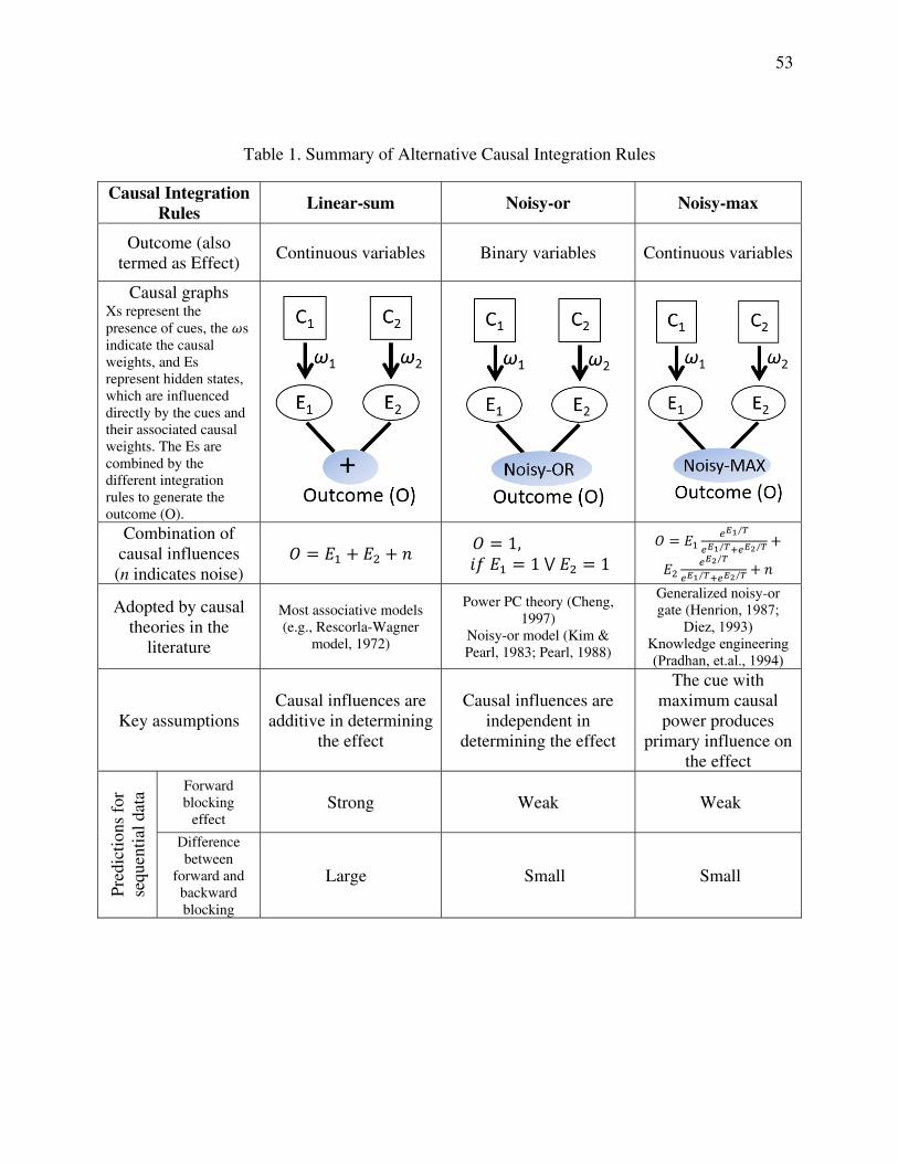
53
Table 1. Summary of Alternative Causal Integration Rules
Causal Integration Rules Linear-sum Noisy-or Noisy-max
Outcome (also termed as Effect)
Continuous variables Binary variables Continuous variables
Causal graphs Xs represent the presence of cues, the s indicate the causal weights, and Es represent hidden states, which are influenced directly by the cues and their associated causal weights. The Es are combined by the different integration rules to generate the outcome (O).
Combination of causal influences (n indicates noise)
1,
1 ⋁ 1
⁄
⁄ ⁄⁄
⁄ ⁄
Adopted by causal theories in the
literature
Most associative models (e.g., Rescorla-Wagner
model, 1972)
Power PC theory (Cheng, 1997)
Noisy-or model (Kim & Pearl, 1983; Pearl, 1988)
Generalized noisy-or gate (Henrion, 1987;
Diez, 1993) Knowledge engineering (Pradhan, et.al., 1994)
Key assumptions Causal influences are
additive in determining the effect
Causal influences are independent in
determining the effect
The cue with maximum causal power produces
primary influence on the effect
Pred
icti
ons
for
sequ
entia
l dat
a Forward blocking
effect Strong
Weak
Weak
Difference between
forward and backward blocking
Large Small Small

54
Table 2. Experimental Design and Simulation Results for Vandorpe and De Houwer (2005)
Paradigms Stage 1
6 trials Stage 2 6 trials
Test Human rating Model prediction Noisy-or Linear-sum
Forward blocking A+ AX+ A 9.9 8.8 9.8 X 5.0 5 1.3
Reduced overshadowing
A- AX+ A 1.2 2.5 5.2 X 9.4 8.8 5.8
Control AX+ A 5.4 4.3 5.6 X 5.6 4.4 5.4
Rating scale: 1 to 10; human data for blocked cue X in bold
Table 3. Experimental Design and Simulation Results for Wasserman and Berglan (2010)
Paradigms Stage 1 30 trials
Stage 2 30 trials
Test Human rating Model prediction Noisy-or Linear-sum
Backward blocking AX+ A+ A 8.81 8.5 9.0 X 4.75 5.2 1.7
Recovery from overshadowing
AX+ A- A 1.35 1.5 1.0 X 6.81 7.0 8.4
Rating scale: 1 to 9; human data for blocked cue X in bold

55
Table 4. Experimental Design in Pre-training Paradigm (Beckers et al., 2005)
Experiment Group Phase 1: pre-training Phase 2 Phase 3 Test
Exp2 additive 8G+ /8H+ /8GH++ 8A+ 8AX+ /8KL+ A, X, K, L subadditive 8G+ /8H+ /8GH+ 8A+ 8AX+ /8KL+ A, X, K, L
Exp3 additive 8G+ /8H+ /8GH++ 8AX+ /8KL+ 8A+ A, X, K, L subadditive 8G+ /8H+ /8GH+ 8AX+ /8KL+ 8A+ A, X, K, L
Note A, X, K, L, G and H are different food cues; + and ++ indicate moderate and strong allergic reactions as outcome. The numerical values indicate the number of trials.
Table 5. Experimental Design in Post-training Paradigm (Beckers et al., 2005)
Experiment Group Phase 1 Phase 2 Phase 3: post-training Test
Exp4 additive 8A+ 8AX+ /8KL+ 8G+ /8H+ /8GH++ A, X, K, L subadditive 8A+ 8AX+ /8KL+ 8G+ /8H+ /8GH+ A, X, K, L
Note A, X, K, L, G and H are different food cues; + and ++ indicate moderate and strong allergic reactions as outcome. The numerical values indicate the number of trials.
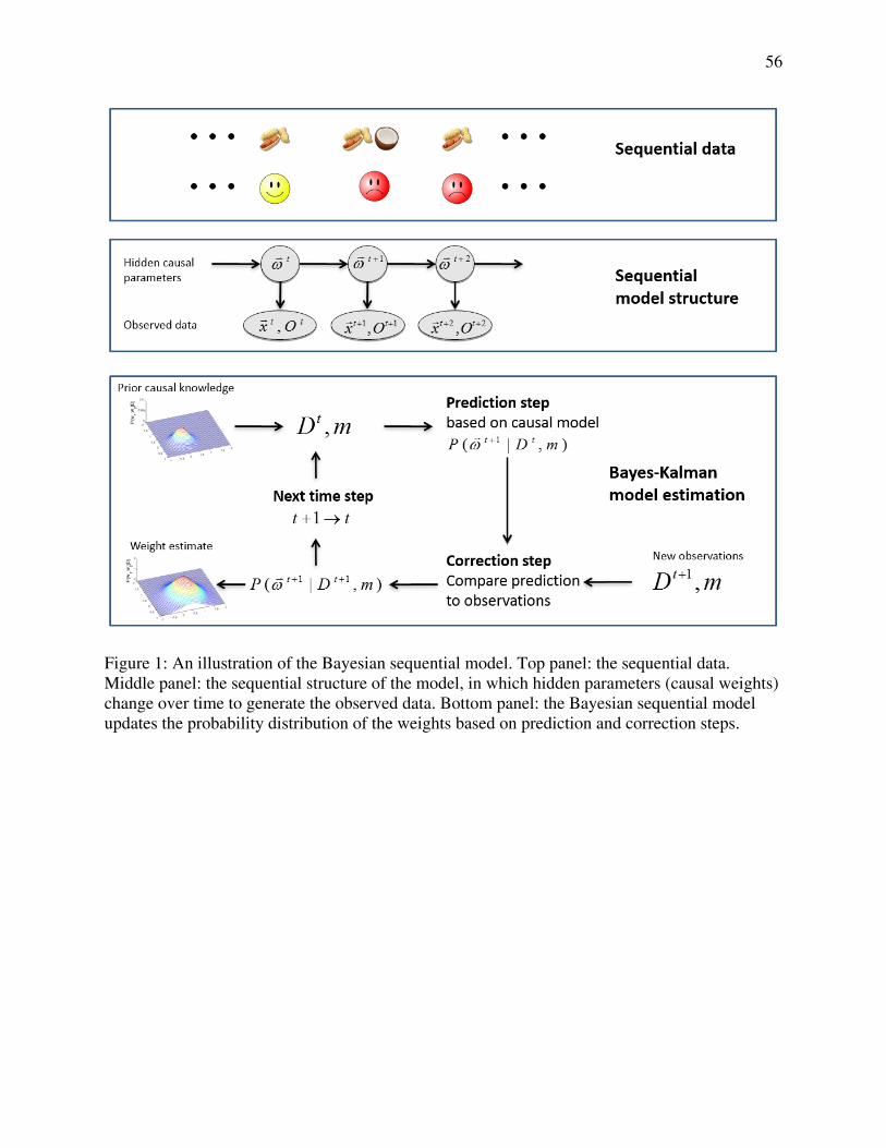
56
Figure 1: An illustration of the Bayesian sequential model. Top panel: the sequential data. Middle panel: the sequential structure of the model, in which hidden parameters (causal weights) change over time to generate the observed data. Bottom panel: the Bayesian sequential model updates the probability distribution of the weights based on prediction and correction steps.
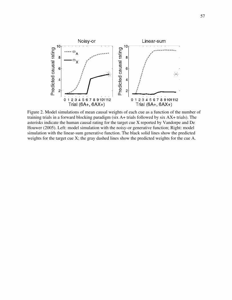
57
Figure 2. Model simulations of mean causal weights of each cue as a function of the number of training trials in a forward blocking paradigm (six A+ trials followed by six AX+ trials). The asterisks indicate the human causal rating for the target cue X reported by Vandorpe and De Houwer (2005). Left: model simulation with the noisy-or generative function; Right: model simulation with the linear-sum generative function. The black solid lines show the predicted weights for the target cue X; the gray dashed lines show the predicted weights for the cue A.

58
Figure 3. Comparison of human causal ratings with model predictions for five experimental paradigms. Humans (top) show different blocking effects in different paradigms. Note that human ratings have been linearly transformed to the same scale range of [1, 10] for all five studies. These differences are well captured by the model based on the noisy-or function (middle), but less so by the model based on the linear-sum rule (bottom).

59
Figure 4. Log-likelihood ratios of model evidence for the noisy-max model relative to the linear-sum model in the pre-training phase by Beckers et al. (2005). A positive ratio value supports a noisy-max model, and a negative value indicate that a linear-sum model provides better account to the observations. The model selection procedure chooses the linear-sum model for the additive condition, but chooses the noisy-max model for the subadditive condition. The error bars indicate the standard deviation based on ten runs of simulations.
noisy‐max
linear‐sum
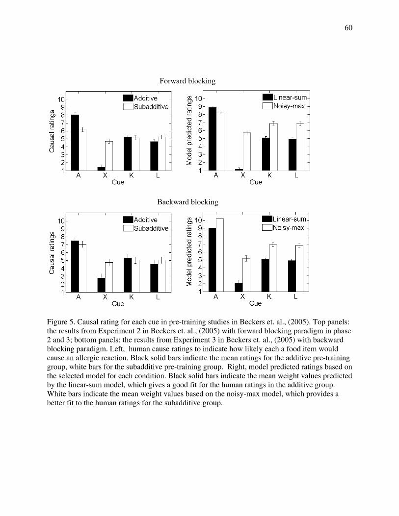
60
Figure 5. Causal rating for each cue in pre-training studies in Beckers et. al., (2005). Top panels: the results from Experiment 2 in Beckers et. al., (2005) with forward blocking paradigm in phase 2 and 3; bottom panels: the results from Experiment 3 in Beckers et. al., (2005) with backward blocking paradigm. Left, human cause ratings to indicate how likely each a food item would cause an allergic reaction. Black solid bars indicate the mean ratings for the additive pre-training group, white bars for the subadditive pre-training group. Right, model predicted ratings based on the selected model for each condition. Black solid bars indicate the mean weight values predicted by the linear-sum model, which gives a good fit for the human ratings in the additive group. White bars indicate the mean weight values based on the noisy-max model, which provides a better fit to the human ratings for the subadditive group.
Forward blocking
Backward blocking
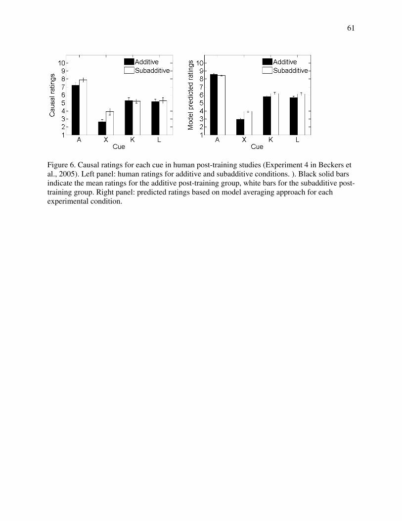
61
Figure 6. Causal ratings for each cue in human post-training studies (Experiment 4 in Beckers et al., 2005). Left panel: human ratings for additive and subadditive conditions. ). Black solid bars indicate the mean ratings for the additive post-training group, white bars for the subadditive post-training group. Right panel: predicted ratings based on model averaging approach for each experimental condition.

62
Figure 7. Human data and simulation results for the primacy effect reported in Experiment 1 of Dennis and Ahn (2001). The primacy effect is demonstrated by the results the final causal judgment is positive when the generative causal sequence is presented first in the +/- experimental condition, but negative when the preventive causal sequence is presented first in the -/+ experimental condition. Error bars indicate standard deviation. For model results, the error bars were calculated based on ten runs of simulations.
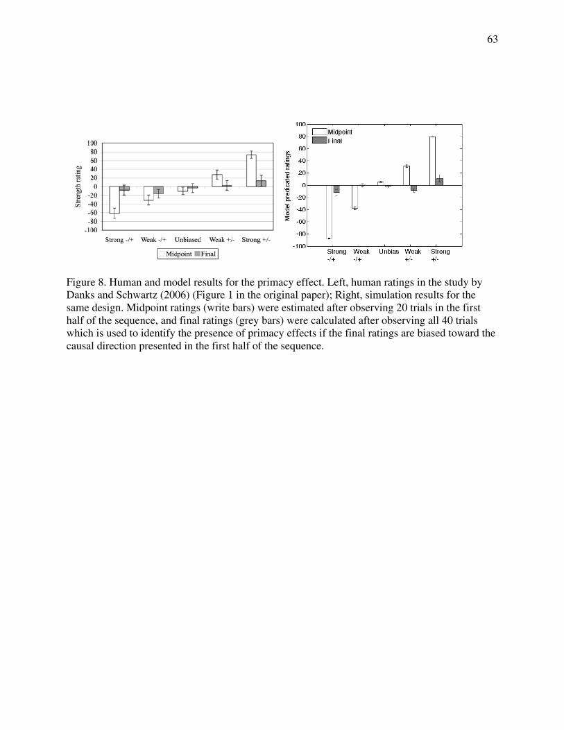
63
Figure 8. Human and model results for the primacy effect. Left, human ratings in the study by Danks and Schwartz (2006) (Figure 1 in the original paper); Right, simulation results for the same design. Midpoint ratings (write bars) were estimated after observing 20 trials in the first half of the sequence, and final ratings (grey bars) were calculated after observing all 40 trials which is used to identify the presence of primacy effects if the final ratings are biased toward the causal direction presented in the first half of the sequence.