A Bayesian software for phylogenetic reconstruction using...
40
PhyloBayes A Bayesian software for phylogenetic reconstruction using mixture models Nicolas Lartillot, Samuel Blanquart, Thomas Lepage [email protected] Version 4.1, June, 2015 1
Transcript of A Bayesian software for phylogenetic reconstruction using...
PhyloBayes
A Bayesian software for phylogenetic reconstruction
using mixture models
Nicolas Lartillot, Samuel Blanquart, Thomas Lepage
Version 4.1, June, 2015
1
Contents
1 Introduction 3
1.1 Modeling site-specific effects using non-parametric methods . . . . . . . . . . 3
1.2 Empirical mixture models . . . . . . . . . . . . . . . . . . . . . . . . . . . . . 4
1.3 Phylogenetic reconstruction . . . . . . . . . . . . . . . . . . . . . . . . . . . . 4
1.4 Molecular dating . . . . . . . . . . . . . . . . . . . . . . . . . . . . . . . . . . 5
1.5 Choosing a model . . . . . . . . . . . . . . . . . . . . . . . . . . . . . . . . . . 5
2 Input data format 7
2.1 Sequences . . . . . . . . . . . . . . . . . . . . . . . . . . . . . . . . . . . . . . 7
2.2 Trees . . . . . . . . . . . . . . . . . . . . . . . . . . . . . . . . . . . . . . . . . 7
2.3 Outgroups . . . . . . . . . . . . . . . . . . . . . . . . . . . . . . . . . . . . . . 8
2.4 Calibrations . . . . . . . . . . . . . . . . . . . . . . . . . . . . . . . . . . . . . 8
3 General presentation of the programs 10
3.1 Running a chain (pb) . . . . . . . . . . . . . . . . . . . . . . . . . . . . . . . . 11
3.2 Checking convergence and mixing (bpcomp and tracecomp) . . . . . . . . . . 12
3.3 Obtaining posterior consensus trees and parameter estimates . . . . . . . . . 13
4 Divergence times 14
4.1 A brief example . . . . . . . . . . . . . . . . . . . . . . . . . . . . . . . . . . . 14
5 Detailed options 16
5.1 pb . . . . . . . . . . . . . . . . . . . . . . . . . . . . . . . . . . . . . . . . . . 16
5.2 bpcomp . . . . . . . . . . . . . . . . . . . . . . . . . . . . . . . . . . . . . . . . 25
5.3 readpb . . . . . . . . . . . . . . . . . . . . . . . . . . . . . . . . . . . . . . . . 26
5.4 readdiv . . . . . . . . . . . . . . . . . . . . . . . . . . . . . . . . . . . . . . . 26
5.5 ppred . . . . . . . . . . . . . . . . . . . . . . . . . . . . . . . . . . . . . . . . 27
5.6 ancestral . . . . . . . . . . . . . . . . . . . . . . . . . . . . . . . . . . . . . . 29
6 Cross-Validation 32
7 Priors 35
2
1 Introduction
PhyloBayes is a Bayesian Markov chain Monte Carlo (MCMC) sampler for phylogenetic
inference. The program will perform phylogenetic reconstruction using either nucleotide,
protein, or codon sequence alignments. Compared to other phylogenetic MCMC samplers,
the main distinguishing feature of PhyloBayes is the use of non-parametric methods for
modeling among-site variation in nucleotide or amino-acid propensities.
PhyoBayes3.4, implements several probabilistic models:
• non-parametric models of site-specific rates, equilibrium frequency profiles or substi-
tution matrices, using Dirichlet processes.
• Tuffley and Steel’s covarion model (Tuffley and Steel, 1998), as well as the mixture of
branch length (mbl) models (Kolaczkowski and Thornton, 2008; Zhou et al., 2007).
• empirical mixtures of profiles, or of matrices.
• auto-correlated and non auto-correlated relaxed clocks for molecular dating
1.1 Modeling site-specific effects using non-parametric methods
Among-site variation in the rate of substitution is often modeled using a gamma distribution.
Doing so, however, only models variation in the rate of evolution, and does not account for
the fact that the different nucleotides or amino-acids might have uneven propensities across
positions.
As a way of modeling state propensity variation along sequences, in PhyloBayes, the
rate and also a profile—controlling nucleotide or amino acid equilibrium frequencies associ-
ated with the substitution process—are modeled as site-specific random variables. As has
been shown in several previous works, accounting for such generalized among-site variation
results in a better statistical fit and greater phylogenetic accuracy. Of particular interest
to phylogenetic reconstruction, such models show a greater robustness to systematic errors
such as long-branch attraction problems.
There are two ways site-specific propensities can be modeled. First, one can use a
parametric model. In such models, the parametric form of the law describing the distribution
of the site-specific feature under investigation is assumed known, up to a few parameters
that will be estimated from the data. The best example is the use of a gamma distribution
for modeling the distribution of relative rates of substitution across sites (Yang, 1994).
3
Alternatively, one can use non-parametric models: the overall shape of the distribution
across sites is not specified a priori but is directly inferred from the data. It is thus more gen-
eral than the parametric method. There are different non-parametric methods. A practical
approach, often adopted in Bayesian inference, is the use of Dirichlet process mixtures (Fer-
guson, 1973). Formally, these are infinite mixtures, i.e. mixtures with a countably infinite
number of components.
PhyloBayes uses Dirichlet processes for modeling sites-specific profiles (Lartillot and
Philippe, 2004). Each site is thus given a frequency vector profile over the 20 amino-acids
or the 4 bases. These are combined with a globally defined set of exchange rates, so as to
yield site-specific substitution processes. The global exchange rates can be fixed to uniform
values (the CAT-Poisson, or more simply CAT, settings), to empirical estimates (e.g. JTT,
WAG or LG) or inferred from the data (CAT-GTR settings).
1.2 Empirical mixture models
The non-parametric models introduced above are flexible. They automatically estimate the
distribution of site-specific effects underlying each dataset. But on the other hand, they may
require a relatively large amount of data for reliable estimation.
An alternative that would be suitable for smaller alignments is offered by the so-called
empirical mixture models. Unlike non-parametric mixtures, empirical models have a fixed,
pre-determined set of components, which have been estimated on a large database of multiple
sequence alignments. Classical empirical matrices, such as JTT, WAG and LG (Le and
Gascuel, 2008) are a specific case of empirical model, with only one component. A few years
ago, empirical mixtures of profiles were proposed (Quang et al., 2008; Wang et al., 2008),
which are implemented in the current version of PhyloBayes. The user can also specify its
own custom set of exchange rates or mixture of profiles.
1.3 Phylogenetic reconstruction
Samples approximately from the posterior distribution are obtained by Markov chain Monte
Carlo (MCMC) and are then used to estimate marginal distributions, or expectations, over
the parameters of interest. Concerning the topology of the phylogenetic tree, PhyloBayes
works like usual Bayesian phylogenetic reconstruction programs and outputs a majority-rule
posterior consensus tree. Conversely, one may be interested in the site-specific biochemical
specificities that have been captured by the infinite mixture model, in which case mean
4
posterior site-specific profiles will be estimated from the MCMC output.
1.4 Molecular dating
PhyloBayes can be used for Bayesian molecular dating using relaxed molecular clocks. Sev-
eral alternative clock relaxation models are available, including the log-normal (Brownian)
auto-correlated model of Thorne et al. (1998), the CIR process of Lepage et al. (2007) and
uncorrelated clocks (Drummond et al., 2006). Fossil calibrations can be provided as hard
constraints (Kishino et al., 2001) or as soft constraints (Yang and Rannala, 2006).
1.5 Choosing a model
It is still difficult to get a general idea of the relative merits of the models, as it depends
on the dataset and on the criterion used to measure the fit. But a few trends are observed,
which can be used for establishing general guidelines.
1.5.1 Amino acid replacement models
Except for small datasets (less than 400 aligned positions), CAT-GTR is virtually always
the model with highest fit among all models implemented in PhyloBayes. The CAT-Poisson
model, which was the model initially developed in Lartillot and Philippe (2004), is less fit
than CAT-GTR but generally more fit than single-matrix models on large and datasets,
particularly when mutational saturation (multiple substitutions) is prevalent.
Concerning the posterior consensus tree, both CAT-GTR and CAT-Poisson are signif-
icantly more robust against long-branch attraction (LBA) artifacts, compared to all other
models. However, in some cases, there are differences between the topologies obtained under
CAT or CAT-GTR. The flat exchange rates of CAT (which were introduced mostly for the
sake of computational efficiency) are not biologically realistic, suggesting that CAT-GTR
would generally be a better option.
Empirical mixture models (C60 or WLSR5) may be appropriate for single gene datasets.
1.5.2 Nucleotide substitution models
The CAT-GTR model is a very good generic model also for DNA or RNA data, again
probably better than CAT (which does not correctly handle differences in transition and
transversion rates) but also, in most cases, better than classical nucleotide substitution
models.
5
1.5.3 Rate across sites
PhyloBayes implements several models of rate variation across sites: the discrete gamma
distribution (default model), the continuous gamma distribution and a Dirichlet process
over site-specific rates (Huelsenbeck and Suchard, 2007).
The Dirichlet process appears to have a better fit than the more classical discrete gamma
distribution with 4 categories. On the other hand, it may sometimes result in MCMC
convergence and mixing difficulties (also true for the continuous gamma model). Thus far,
we have not seen many cases where the Dirichlet process over the rates was resulting in a
significantly different phylogeny, compared to the discrete gamma model.
1.5.4 Dataset size
In practice, the Dirichlet process mixture works best for alignments in the range of 1 000
to 20 000 aligned positions. Beyond 20 000 positions, convergence and mixing of the Monte
Carlo progressively become challenging. As for the number of taxa, the MCMC sampler
seems able to deal alignments with up to 100 taxa reasonably well.
A possible approach for analyzing very large multi-gene datasets (large in terms of the
number of aligned positions) is to perform jackknife resampling procedures (although resam-
pling procedures are not so easily justified from a Bayesian philosophical standpoint.). An
example of gene-jackknife using PhyloBayes is described in Delsuc et al. (2008).
6
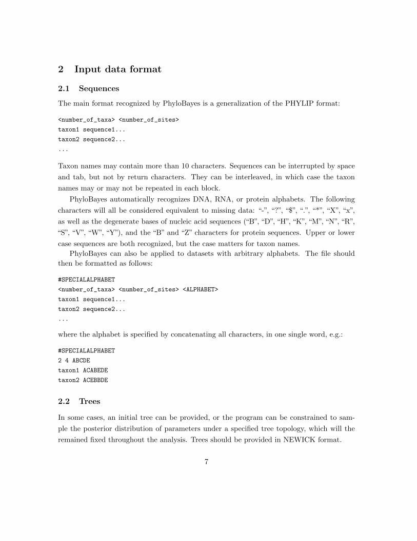
2 Input data format
2.1 Sequences
The main format recognized by PhyloBayes is a generalization of the PHYLIP format:
<number_of_taxa> <number_of_sites>
taxon1 sequence1...
taxon2 sequence2...
...
Taxon names may contain more than 10 characters. Sequences can be interrupted by space
and tab, but not by return characters. They can be interleaved, in which case the taxon
names may or may not be repeated in each block.
PhyloBayes automatically recognizes DNA, RNA, or protein alphabets. The following
characters will all be considered equivalent to missing data: “-”, “?”, “$”, “.”, “*”, “X”, “x”,
as well as the degenerate bases of nucleic acid sequences (“B”, “D”, “H”, “K”, “M”, “N”, “R”,
“S”, “V”, “W”, “Y”), and the “B” and “Z” characters for protein sequences. Upper or lower
case sequences are both recognized, but the case matters for taxon names.
PhyloBayes can also be applied to datasets with arbitrary alphabets. The file should
then be formatted as follows:
#SPECIALALPHABET
<number_of_taxa> <number_of_sites> <ALPHABET>
taxon1 sequence1...
taxon2 sequence2...
...
where the alphabet is specified by concatenating all characters, in one single word, e.g.:
#SPECIALALPHABET
2 4 ABCDE
taxon1 ACABEDE
taxon2 ACEBBDE
2.2 Trees
In some cases, an initial tree can be provided, or the program can be constrained to sam-
ple the posterior distribution of parameters under a specified tree topology, which will the
remained fixed throughout the analysis. Trees should be provided in NEWICK format.
7
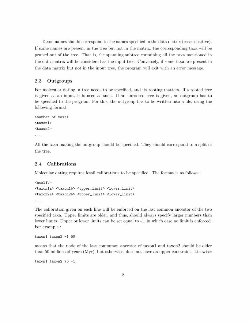
Taxon names should correspond to the names specified in the data matrix (case sensitive).
If some names are present in the tree but not in the matrix, the corresponding taxa will be
pruned out of the tree. That is, the spanning subtree containing all the taxa mentioned in
the data matrix will be considered as the input tree. Conversely, if some taxa are present in
the data matrix but not in the input tree, the program will exit with an error message.
2.3 Outgroups
For molecular dating, a tree needs to be specified, and its rooting matters. If a rooted tree
is given as an input, it is used as such. If an unrooted tree is given, an outgroup has to
be specified to the program. For this, the outgroup has to be written into a file, using the
following format:
<number of taxa>
<taxon1>
<taxon2>
...
All the taxa making the outgroup should be specified. They should correspond to a split of
the tree.
2.4 Calibrations
Molecular dating requires fossil calibrations to be specified. The format is as follows:
<ncalib>
<taxon1a> <taxon1b> <upper_limit> <lower_limit>
<taxon2a> <taxon2b> <upper_limit> <lower_limit>
...
The calibration given on each line will be enforced on the last common ancestor of the two
specified taxa. Upper limits are older, and thus, should always specify larger numbers than
lower limits. Upper or lower limits can be set equal to -1, in which case no limit is enforced.
For example ;
taxon1 taxon2 -1 50
means that the node of the last commmon ancestor of taxon1 and taxon2 should be older
than 50 millions of years (Myr), but otherwise, does not have an upper constraint. Likewise:
taxon1 taxon2 70 -1
8

only specifies an upper constraint of 70 Myr, and no lower constraint. And finally:
taxon1 taxon2 70 50
specifies an upper and a lower constraint, thus the interval [50,70] Myr.
For a node that has both an upper and a lower constraint, it is important to specify both
on the same line, thus as:
taxon1 taxon2 70 50
and not
taxon1 taxon2 -1 50
taxon1 taxon2 70 -1
9

3 General presentation of the programs
PhyloBayes is provided both as executable files (for linux x86-64) and as a C++ source code.
Depending on the operating system running on your cluster, you may need to recompile the
code. To this end, a simple Makefile is provided in the sources directory, and compiling with
the make command should then work in most simple situations.
The CIR clock relaxation model (Lepage et al., 2007) requires functions from the gsl
library. To make compiling as simple as possible, the CIR model is deactivated by default.
In order to use this model, one should first uncomment a compilation instruction in the
Makefile (at the very beginning of the file, remove the # in front of USE_GSL=-DGSL). This
of course requires gsl to be installed on your machine.
The general philosophy of PhyloBayes is rather ’unixy’: instead of having one single pro-
gram that does everything, through standard input and output streams (i.e. keyboard and
screen), several small programs have been written, working more or less like unix commands
using input and output files. The detailed model and Monte Carlo settings can be controlled
through options, starting with -.
Specifically, the following programs can be found in the package (for details about any
of these programs, type the name without arguments):
• pb : the MCMC sampler.
• readpb : post-analysis program, for computing a variety of posterior averages.
• bpcomp : evaluates the discrepancy of bipartition frequencies between two or more
independent runs and computes a consensus by pooling the trees of all the runs being
compared.
• tracecomp : evaluates the discrepancy between two or more independent runs based
on the summary variables provided in the trace files.
• ppred : posterior predictive analyses.
• readdiv : post-analysis program for relaxed clock analyses.
• ancestral : estimation of ancestral sequences and substitution histories.
• cvrep/readcv/sumcv : model comparison by cross-validation.
In this section, a rapid tour of the programs is proposed. A more detailed explanation
of all available options for each program is given in the next section.
10

3.1 Running a chain (pb)
A run of the pb program will produce a series of points drawn from the posterior distribution
over the parameters of the model. Each point defines a detailed model configuration (tree
topology, branch lengths, nucleotide or amino-acid profiles of the mixture, etc.). The series
of points defines a chain. To run the program:
pb -d <dataset> <chainname>
The -d option is for specifying the dataset. Many other options are available for speci-
fying the model (see below). The default options are the CAT-Poisson model with discrete
gamma (4 categories). Before starting, the chain will output a summary of the settings.
A series of files will be produced with a variety of extensions. The most important are:
• <name>.treelist: list of sampled trees;
• <name>.trace: the trace file, containing a few relevant summary statistics (log-likelihood,
total length of the tree, number of components in the mixture, etc).
• <name>.chain: this file contains the detailed parameter configurations visited during
the run and is used by readpb for computing posterior averages.
The chains will run as long as allowed. They can be interrupted at any time and then
restarted, in which case they will resume from the last check-point (last point saved before
the interruption). To soft-stop a chain, use stoppb:
stoppb <chainname>
Alternatively, you can open the <name>.run file and replace the 1 by a 0. Under linux, this
can be done with the simple following command:
echo 0 > <chainname>.run
The chain will finish the current cycle before exiting. To restart an already existing chain:
pb <chainname>
Be careful not to restart an already running chain.
11
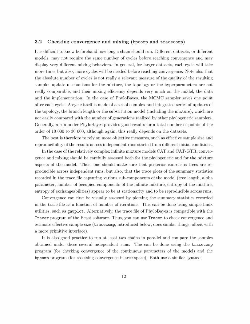
3.2 Checking convergence and mixing (bpcomp and tracecomp)
It is difficult to know beforehand how long a chain should run. Different datasets, or different
models, may not require the same number of cycles before reaching convergence and may
display very different mixing behaviors. In general, for larger datasets, each cycle will take
more time, but also, more cycles will be needed before reaching convergence. Note also that
the absolute number of cycles is not really a relevant measure of the quality of the resulting
sample: update mechanisms for the mixture, the topology or the hyperparameters are not
really comparable, and their mixing efficiency depends very much on the model, the data
and the implementation. In the case of PhyloBayes, the MCMC sampler saves one point
after each cycle. A cycle itself is made of a set of complex and integrated series of updates of
the topology, the branch length or the substitution model (including the mixture), which are
not easily compared with the number of generations realized by other phylogenetic samplers.
Generally, a run under PhyloBayes provides good results for a total number of points of the
order of 10 000 to 30 000, although again, this really depends on the datasets.
The best is therefore to rely on more objective measures, such as effective sample size and
reproducibility of the results across independent runs started from different initial conditions.
In the case of the relatively complex infinite mixture models CAT and CAT-GTR, conver-
gence and mixing should be carefully assessed both for the phylogenetic and for the mixture
aspects of the model. Thus, one should make sure that posterior consensus trees are re-
producible across independent runs, but also, that the trace plots of the summary statistics
recorded in the trace file capturing various sub-components of the model (tree length, alpha
parameter, number of occupied components of the infinite mixture, entropy of the mixture,
entropy of exchangeabilities) appear to be at stationarity and to be reproducible across runs.
Convergence can first be visually assessed by plotting the summary statistics recorded
in the trace file as a function of number of iterations. This can be done using simple linux
utilities, such as gnuplot. Alternatively, the trace file of PhyloBayes is compatible with the
Tracer program of the Beast software. Thus, you can use Tracer to check convergence and
estimate effective sample size (tracecomp, introduced below, does similar things, albeit with
a more primitive interface).
It is also good practice to run at least two chains in parallel and compare the samples
obtained under these several independent runs. The can be done using the tracecomp
program (for checking convergence of the continuous parameters of the model) and the
bpcomp program (for assessing convergence in tree space). Both use a similar syntax:
12

bpcomp -x 1000 10 <chain1> <chain2>
Here, using a burn-in of 1000, and sub-sampling every 10 trees, the bpcomp program will
output the largest (maxdiff) and mean (meandiff) discrepancy observed across all biparti-
tions. It will also produce a file (bpcomp.con.tre) with the consensus obtained by pooling
all the trees of the chains given as arguments.
Note that bpcomp can be run on a single chain (in which case it will simply produce
the consensus of all trees after burn-in). However, using bpcomp on multiple chains usually
results in more stable MCMC estimates of the posterior consensus tree.
Some guidelines:
• maxdiff < 0.1: good run.
• maxdiff < 0.3: acceptable: gives a good qualitative picture of the posterior consensus.
• 0.3 < maxdiff < 1: the sample is not yet sufficiently large, and the chains have not
converged, but this is on the right track.
• if maxdiff = 1 even after 10,000 points, this indicates that at least one of the runs is
stuck in a local maximum.
Similarly,
tracecomp -x 1000 <chain1> <chain2>
will produce an output summarizing the discrepancies and the effective sizes estimated for
each column of the trace file. The discrepancy d is defined as d = 2|µ1 − µ2|/(σ1 + σ2),
where µi is the mean and σi the standard deviation associated with a particular column and
i runs over the chains. The effective size is evaluated using the method of Geyer (1992). The
guidelines are:
• maxdiff < 0.1 and minimum effective size > 300: good run;
• maxdiff < 0.3 and minimum effective size > 50: acceptable run.
3.3 Obtaining posterior consensus trees and parameter estimates
The readpb program is meant for estimating some key parameters of the model. As a simple
example:
readpb -x 1000 10 <chainname>
13

will take one tree every ten, discarding the first 1000 trees. It will produce several
additional files:
• <chainname>_sample.general, containing a few general statistical averages (mean
posterior log likelihood, tree length, alpha parameter, number of modes, etc.)
• <chainname>_sample.con.tre : the majority-rule posterior consensus tree
• <chainname>_sample.bplist : the list of weighted bipartitions.
Various options allow one to compute several other posterior averages, such as site-specific
rates and equilibrium frequency profiles (see below, detailed options).
4 Divergence times
PhyloBayes allows for molecular dating under several alternative relaxed clock models and
priors on divergence times. In the following, we give a brief presentation of this feature of
the program, while emphasizing the most important points to be careful about.
4.1 A brief example
Using PhyloBayes, molecular dating only works under a fixed topology, which has to be
specified using the -T option. The molecular dating option of pb is activated by specifying
a model of clock relaxation or by specifying calibrations. Here is an example, taken from
Douzery et al. (2004). Files are in the data/moc directory:
pb -d moc.ali -T moc.tree -r bikont.outgroup -cal calib -ln -rp 2000 2000 mocln1
Here, the program is given a protein sequence alignment (-d moc.ali), a tree file (-T
moc.tree), an outgroup (-r bikont.outgroup, imposing a basal split between unikonts
and bikonts), and a file containing 6 fossil calibrations (-cal calib) specified in millions
of years. A log-normal autocorrelated relaxed clock (-ln) is assumed, together with a uni-
form prior on divergence times (default prior). A gamma prior of mean 2000 and standard
deviation 2000 Myr (thus, an exponential of mean 2000 Myr) is specified for the age of the
root.
PhyloBayes provides several relaxed clock models, either autocorrelated, such as the
log normal clock (Thorne et al., 1998) or or the CIR process (Lepage et al., 2007), or
uncorrelated, such as the white noise process (Lepage et al., 2007) or the uncorrelated
14
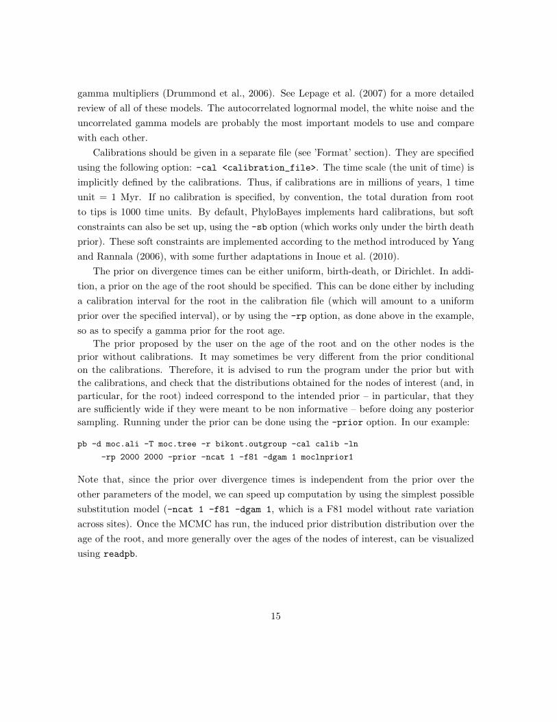
gamma multipliers (Drummond et al., 2006). See Lepage et al. (2007) for a more detailed
review of all of these models. The autocorrelated lognormal model, the white noise and the
uncorrelated gamma models are probably the most important models to use and compare
with each other.
Calibrations should be given in a separate file (see ’Format’ section). They are specified
using the following option: -cal <calibration_file>. The time scale (the unit of time) is
implicitly defined by the calibrations. Thus, if calibrations are in millions of years, 1 time
unit = 1 Myr. If no calibration is specified, by convention, the total duration from root
to tips is 1000 time units. By default, PhyloBayes implements hard calibrations, but soft
constraints can also be set up, using the -sb option (which works only under the birth death
prior). These soft constraints are implemented according to the method introduced by Yang
and Rannala (2006), with some further adaptations in Inoue et al. (2010).
The prior on divergence times can be either uniform, birth-death, or Dirichlet. In addi-
tion, a prior on the age of the root should be specified. This can be done either by including
a calibration interval for the root in the calibration file (which will amount to a uniform
prior over the specified interval), or by using the -rp option, as done above in the example,
so as to specify a gamma prior for the root age.
The prior proposed by the user on the age of the root and on the other nodes is the
prior without calibrations. It may sometimes be very different from the prior conditional
on the calibrations. Therefore, it is advised to run the program under the prior but with
the calibrations, and check that the distributions obtained for the nodes of interest (and, in
particular, for the root) indeed correspond to the intended prior – in particular, that they
are sufficiently wide if they were meant to be non informative – before doing any posterior
sampling. Running under the prior can be done using the -prior option. In our example:
pb -d moc.ali -T moc.tree -r bikont.outgroup -cal calib -ln
-rp 2000 2000 -prior -ncat 1 -f81 -dgam 1 moclnprior1
Note that, since the prior over divergence times is independent from the prior over the
other parameters of the model, we can speed up computation by using the simplest possible
substitution model (-ncat 1 -f81 -dgam 1, which is a F81 model without rate variation
across sites). Once the MCMC has run, the induced prior distribution distribution over the
age of the root, and more generally over the ages of the nodes of interest, can be visualized
using readpb.
15

5 Detailed options
5.1 pb
5.1.1 General options
-d <datafile>
specifies the multiple sequence alignment to be analyzed.
-dc
constant sites are removed. Note that the likelihood will not be properly conditioned on
this removal, as it normally should be (as explained by Lewis, 2001). Using this option is
therefore problematic.
-t <treefile>
forces the chain to start from the specified tree.
-T <treefile>
forces the chain to run under a fixed topology (as specified in the given file). In other words,
the chain only samples from the posterior distribution over all other parameters (branch
lengths, alpha parameter, etc.), conditional on the specified topology. This should be a
bifurcating tree (see Input Data Format section).
-r <outgroup>
roots the tree using the specified outgroup. Current substitution models implemented in
PhyloBayes are reversible, so this rooting option is useful only for clock models.
-s
by default, pb only saves the trees explored by the chain during MCMC. This is enough if
the aim is to infer the tree topology. However, for a more detailed analysis, such as inferring
site-specific rates or equilibrium frequency profiles, conducting cross-validation or posterior
predictive checks, the complete parameter configurations visited by the MCMC should be
saved. This can be done using the -s option. Fixed topology analyses (using the -T option)
will automatically activate this option.
16

-f
forces the program to overwrite an already existing chain with same name.
-x <every> [<until>]
specifies the saving frequency and (optional) the number of points after which the chain
should stop. If <until> is not specified, the chain will run as long as desired. By definition,
-x 1 corresponds to the default saving frequency. In some cases, samples may be strongly
correlated, in which case, if disk space or access is limiting, it would make sense to save
points less frequently, say 10 times less often: to do this, one can use the -x 10 option.
5.1.2 Prior on branch lengths
-lexp
prior on branch lengths is a product of i.i.d. exponential distributions.
-lgam
prior on branch lengths is a product of i.i.d. gamma distributions (more flexible than the
exponential, as it allows independent control of the mean and the variance of the distribution
on branch lengths).
-meanlength <meanlength>
fixes the mean of the exponential (or gamma) priors to the specified value. Without this
command, this mean is considered as a free parameter, endowed with an exponential prior
of mean 0.1. In the case of the gamma prior, the variance/mean ratio is always considered
as a free parameter, with an exponential prior of mean 1.
5.1.3 Rates across sites
-dgam <n>
specifies n categories for the discrete gamma distribution. Setting n = 1 amounts to a model
without across-site variation in substitution rate.
-uni
17
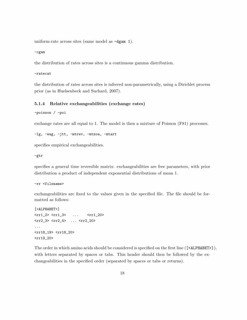
uniform-rate across sites (same model as -dgam 1).
-cgam
the distribution of rates across sites is a continuous gamma distribution.
-ratecat
the distribution of rates across sites is inferred non-parametrically, using a Dirichlet process
prior (as in Huelsenbeck and Suchard, 2007).
5.1.4 Relative exchangeabilities (exchange rates)
-poisson / -poi
exchange rates are all equal to 1. The model is then a mixture of Poisson (F81) processes.
-lg, -wag, -jtt, -mtrev, -mtzoa, -mtart
specifies empirical exchangeabilities.
-gtr
specifies a general time reversible matrix: exchangeabilities are free parameters, with prior
distribution a product of independent exponential distributions of mean 1.
-rr <filename>
exchangeabilities are fixed to the values given in the specified file. The file should be for-
matted as follows:
[<ALPHABET>]
<rr1_2> <rr1_3> ... <rr1_20>
<rr2_3> <rr2_4> ... <rr2_20>
...
<rr18_19> <rr18_20>
<rr19_20>
The order in which amino acids should be considered is specified on the first line ([<ALPHABET>]),
with letters separated by spaces or tabs. This header should then be followed by the ex-
changeabilities in the specified order (separated by spaces or tabs or returns).
18

5.1.5 Profile mixture
-dp (or -cat)
the distribution of equilibrium frequency profiles across sites is inferred non-parametrically,
using a Dirichlet process prior (Lartillot and Philippe, 2004).
-ncat <n>
specifies a mixture of equilibrium frequency profiles of n components; the number of compo-
nents is fixed whereas the weights and profiles are treated as random variables. Fixing the
number of components of the mixture most often results in a poor mixing of the MCMC.
The Dirichlet process usually has a much better mixing behavior.
-catfix <predef>
specifies a mixture of a set of pre-defined profiles (the weights are re-estimated). The ar-
gument <predef> can be either one of the following keywords: C20, C30, C40, C50, C60,
which correspond to empirical profile mixture models (Quang et al., 2008); or WLSR5, which
correspond to the model of Wang et al. (2008). Note that this latter model actually defines
4 empirical profiles, which are then combined with a fifth component made of the empirical
frequencies of the dataset.
-catfix <filename>
specifies a mixture of a set of user-pre-defined profiles, where <filename> is the name of a
file containing a set of profiles specified as follows:
[<ALPHABET>]
<ncat>
<weight> <freq1> <freq2> ... <freq20>
<weight> <freq1> <freq2> ... <freq20>
...
where <ncat> is the number of profiles, and each line following this number should be a set of
21 real numbers, defining a weight, and then a profile of equilibrium frequencies (separated
by spaces or tabs). The order in which amino acids should be considered is specified on the
first line ([<ALPHABET>]), with letters separated by spaces or tabs. Note that the weights
are there only for historical reasons – they are re-estimated anyway.
19
5.1.6 Combining profiles and exchange rates
Any set of exchange rates can be combined with any of the three settings for the mixture. But
the same set of exchange rates will be used by all components of the mixture. For instance,
-cat -gtr makes an infinite mixture model whose components differ by their equilibrium
frequencies but otherwise share the same set of relative exchange rates (themselves consid-
ered as free parameters). As another example, -catfix wlrs5 -jtt defines the Wang et al.
(2008) model: a model with 5 components, each of which is a matrix made from the rela-
tive exchange rates of the JTT matrix, combined with one of the 4 vectors of equilibrium
frequencies defined by Wang et al. (2008), plus one vector of empirical frequencies.
The default model is -cat -poi, that is, a mixture of Poisson (F81) processes. Note that,
if non-Poisson exchange rates are used, the mixture model is automatically deactivated by
default. Thus, for instance, the -gtr option is equivalent to -gtr -ncat 1. In order to use
a Dirichlet process combined with a GTR matrix of exchange rates, one has to explicitly use
the -gtr -cat combination of options.
5.1.7 Matrix mixture models
-qmm
activates the QMM model, which is a mixture of matrices (thus, allowing for distinct sets
of exchange rates and equilibrium frequencies for each component of the mixture). MCMC
mixing is very challenging under this model configuration.
-qmmfix ul2 / -qmmfix ul3
defines the empirical mixture with 2 or 3 components (Le et al., 2008).
-qmmfix <filename>
specifies a custom empirical mixture of matrices, based on a file containing a set of matrices
specified as follows:
[<ALPHABET>]
<ncat>
<weight>
<freq1> <freq2> ... <freq20>
20
<rr1_2> <rr1_3> ... <rr1_20>
<rr2_3> <rr2_4> ... <rr2_20>
...
<rr19_20>
<weight>
<freq1> <freq2> ... <freq20>
<rr1_2> <rr1_3> ... <rr1_20>
<rr2_3> <rr2_4> ... <rr2_20>
...
<rr19_20>
...
As in the case of profile mixtures, one should specify on the first line ([<ALPHABET>]) the
order in which amino acids are considered. Letters should be separated by spaces or tabs.
Then for each component, one should specify, in turn, a weight, an equilibrium frequency
profile, and finally, a set of relative exchange rates (separated by space, tabs or returns).
-fxw
With this option, and using one of the pre-specified mixtures C10 to C60, the weights are
fixed to the values estimated on the training HSSP database. In all other cases (other pre-
specified profile and matrix mixtures, or custom mixtures), the weights are constrained to
be all equal. Otherwise, without the -fxw option, the weights are free parameters (endowed
with a uniform Dirichlet prior).
5.1.8 Heterotachy
-covarion
Tuffley and Steel’s covarion model (Tuffley and Steel, 1998). This model can be combined
with any of the substitution or amino-acid replacement models defined above. However, it
does not work in combination with the -ratecat or -cgam options (only with the -dgam or
-uni options).
-covext
21
a slightly different version of Tuffley and Steel’s covarion model, in which the rate of the site is
applied both to the substitution and to the switching processes. Under the classical covarion
model (-covarion), fast sites make more substitutions when in the on state, compared
to slow sites. However, all sites switch between the on and off states at the same rate.
In contrast, under the covext model, fast sites also switch faster between on and off. In
practice, this means that the rate is simply applied as a multiplier in front of the tensor
product matrix. The advantage of doing this is that it can be combined with any model of
rate variation across sites.
-mmbl
This is a Bayesian non-parametric version of the mixture of branch lengths (MBL) model
(Kolaczkowski and Thornton, 2008; Zhou et al., 2007). Basically a Dirichlet process of vectors
of branch length multipliers. These multipliers are drawn from a gamma distribution, whose
inverse variance (Φ) is itself considered as a free parameter. Convergence is challenging
under this model.
-gbl <partition>
separate (partition) model, with each gene having its own set of branch lengths, which are
obtained by multiplying the global branch lengths by gene-specific branch length multipliers.
These multipliers are drawn from a gamma distribution, whose inverse variance (Φ) is itself
considered as a free parameter. Convergence in the space of topology is challenging under
this model. The partition file should be specified as follows:
<G>
nsite\_1 nsite\_2 ... nsite\_G
where G is the total number of genes, and nsite_g is the number of aligned positions for
gene g.
5.1.9 Relaxed clock models
-cl
strict molecular clock
-ln
log normal (Brownian) autocorrelated clock (Thorne et al., 1998)
22
-cir
CIR process (Lepage et al., 2007)
-wn
white noise process (Lepage et al., 2007)
-ugam
uncorrelated gamma multipliers (Drummond et al., 2006).
5.1.10 Prior on divergence times
-rp <mean> <stdev>
impose a gamma prior with specified mean and standard deviation for the age of the root.
-unitime
uniform prior on divergence times (default option).
-bd [<p1> <p2>]
birth death prior on divergence times. The birth death process (with species sampling) has
three parameters: the birth rate (λ), the death rate (µ) and the sampling fraction (ω). Only
two of these three parameters are identifiable, which we define as p1 = λ− µ and p2 = λω.
The dimension of p1 and p2 is the inverse of a time. Thus, if fossil calibrations are in Myr,
p1 is the net rate of diversification (speciation - extinction) per Myr. If two real numbers
are given, p1 and p2 will be fixed to the specified values. Otherwise, they will be considered
as free parameters.
-bdhyperprior [<mean1> <stdev1> <mean2> <stdev2>]
birth death hyperprior. The two parameters p1 and p2 will be endowed with gamma distri-
butions of means and priors specified by the command. Default values are 10−3 for all four
hyperparameters (i.e. exponential distributions of mean 10−3 for both p1 and p2).
-dir [<chi>]
23

Dirichlet prior. The hyperparameter χ > 0 is such that smaller value of χ result in a larger
variance of the waiting times between successive speciations (χ = 1 reduces to the uniform
prior). This hyperparameter can be fixed to a pre-specified balue (e.g. -chi 0.5). If no
value is given, it will be considered as unknown. Analyses with calibrations require χ to be
specified.
-cal <calibrations>
impose a set of calibrations (see Format section).
-sb
activates the soft bounds option. Soft bounds are implemented as in Yang and Rannala
(2006). By default, a proportion of 0.05 of the total probability mass is allocated outside
the specified bound(s) (which means, 5% on one side, in the cases of the pure lower and
pure upper bounds, and 2.5 % on each side in the case of a combination of lower and upper
bound). This default can be overridden as follows: -sb [<cutoff>].
-lb [<p> <c>]
activates the Cauchy lower bound, such as introduced by Inoue et al. (2010). The p and
c parameters (of the L(t, p, c) function in Paml4.2, see Inoue et al. (2010) and the manual
of Paml4.2, p 44, equation 1 for details) are by default: c = 1 and p = 0.1. Note that
PhyloBayes does not allow for node-specific cutoff, p and c: they will be the same for all
calibrated nodes.
5.1.11 Data recoding
Data can be recoded by using the -recode command :
-recode <recoding_scheme>
Three pre-specified recoding schemes are available:
dayhoff6 (A,G,P,S,T) (D,E,N,Q) (H,K,R) (F,Y,W) (I,L,M,V) (C)
dayhoff4 (A,G,P,S,T) (D,E,N,Q) (H,K,R) (F,Y,W,I,L,M,V) (C= ?)
hp (A,C,F,G,I,L,M,V,W) (D,E,H,K,N,P,Q,R,S,T,Y)
Arbitrary recodings can also be specified, by setting <recoding_scheme> equal to the
name of a file containing a translation table formatted as follows:
24

<AA1> <Letter1>
<AA2> <Letter2>
..
<AA20> <Letter20>
It is possible to propose that a given amino-acid be considered as missing data, by recoding
it as ? (as is done for cysteine in the case of the dayhoff4 recoding).
5.2 bpcomp
-x <burn-in> [<every> <until>]
Defines the burn-in, the sub-sampling frequency, and the size of the samples of trees to be
taken from the chains under comparison. By default, <burn-in> = 0, <every> = 1 and
<until> is equal to the size of the chain. Thus, for instance:
-x 1000
defines a burn-in of 1000,
-x 1000 10
a burn-in of 1000, taking one every 10 trees, up to the end of each chain, and
-x 1000 10 11000
a burn-in of 1000, taking one every 10 trees, up to the 11 000th point of the chains (or less,
if the chains are shorter). If the chain is long enough, this implies a sample size of 1000.
-o <basename>
outputs the results of the comparison in files with the specified base name combined with
several extensions:
• <basename>.bpcomp: summary of the comparison;
• <basename>.bplist: tabulated list of bipartitions (splits) sorted by decreasing dis-
crepancy between the chains;
• <basename>.con.tre: consensus tree based on the merged bipartition list.
-c <cutoff>
tunes the cutoff for the majority rule consensus (posterior probability support under which
nodes are collapsed in the final consensus tree). By default, the cutoff is equal to 0.5.
25

5.3 readpb
-x <burn-in> [<every> <until>]
Defines the burn-in, the sub-sampling frequency, and the size of the samples of trees to be
taken from the chains under comparison. By default, <burn-in> = 0, <every> = 1 and
<until> is equal to the size of the chain (as for bpcomp, see above).
-c <cutoff>
sets the cutoff for the majority rule consensus. By default, the cutoff is equal to 0.5 (see also
bpcomp)
-r
computes the mean posterior rate at each site.
-rr
computes the mean posterior relative exchangeabilities (only if those are free parameters of
the model).
-ss
computes the mean posterior site-specific state equilibrium frequencies.
-m
outputs a histogram approximating the posterior distribution of the number of occupied
components of the Dirichlet process mixture of profiles.
5.4 readdiv
readdiv -x <burn-in> [<every> <until>] [other options] chainname
This program works like readpb. It will output several files:
<chainname>_sample.dates
<chainname>_sample.chronogram
<chainname>_sample.labels
26
-x <burn-in> [<every> <until>]
defines the burn-in, the sub-sampling frequency, and the size of the samples of trees to be
taken from the chain.
-v <burn-in>
verbose output: outputs all dated trees of the sample into a file.
5.5 ppred
Simple posterior predictive checks Posterior predictive model checking is often used
in Bayesian inference (Meng, 1994; Gelman et al., 2004). It has been introduced in Bayesian
phylogenetics by Bollback (2002). The idea is to compare the value of a given summary
statistic S, such as observed on the true dataset (sobs) with the null distribution of S under
the model. Posterior predictive checking can be seen as the Bayesian version of parametric
bootstrapping, in which the model is first fitted to the data by maximum likelihood, and then
replicates of the original dataset are simulated under this maximum likelihood parameter
estimate. The collection of values of S realized over this series of simulations is then seen as
our sample from the null distribution. Posterior predictive checking works similarly, except
that each replicate of the dataset is simulated under a distinct parameter configuration,
which is drawn from the posterior distribution. Thus, unlike parametric boostrapping, the
posterior predictive approach integrates the uncertainty about the parameter in its null
distribution.
In PhyloBayes, posterior predictive checking is implemented using the ppred program.
First, a MCMC should be run on the dataset under the model of interest, using pb. Then,
using ppred, parameter configurations sampled by this MCMC chain (after burnin) are used
to simulate replicates of the original dataset. The summary statistic S is then evaluated on
each of these replicates, giving a sample from the posterior predictive null distribution. The
deviation of sobs from this distribution can be quantified in terms of the mean deviation, the
z-score and a tail area probability (the so-called posterior predictive p-value). In particular,
if sobs is far in the tail of the distribution, this indicates the presence of model violations –
S is not correctly explained by the model.
In practice, once a chain has been obtained using pb, the following command can be
used:
ppred -x <burn-in> [<every> <until>] [additional options] <chainname>
27
Without any of the additional options, this command will produce a series of simulated
replicates of the original dataset, each of which is then written into a separate file. Al-
ternatively, ppred implements a small number of predefined summary statistics, which are
accessible by adding the relevant option to the command shown above. When one of these
options is used, the simulation replicates are not written into files. Instead, ppred directly
computes the test statistics on the observed and the simulated datasets and then outputs
the mean deviation, the z-score and the posterior predictive p-value for the test. These
pre-defined options are now described:
-div
Biochemical specificity. Under this option, the test statistic is the mean number of distinct
amino acids observed at each column (the mean is taken over all the columns). This test
statistic measures how well the site-specific biochemical patterns are accounted for by a
model (Lartillot et al., 2007). Often, standards models such as WAG, JTT or GTR are re-
jected by this statistic, except CAT or CAT-GTR, which are usually not, or weakly, rejected.
-comp
Compositional homogeneity. This test statistic measures the compositional deviation of
each taxon. The deviation is measured as the sum over the 20 amino-acids of the absolute
differences between the taxon-specific and global empirical frequencies. The program also
uses a global statistic, which is the maximum deviation over the taxa.
Mapping-based posterior predictive checks Sometimes, the summary statistic of in-
terest is not just a function of the observed data, but depends on additional features that
have to be imputed. In particular, in the context of phylogenetic analysis, one may often
be interested in statistics that would capture specific features of the complete substitution
history over the tree. This substitution mapping is not observed, although it can be inferred
based on the model itself, using the idea of stochastic mapping (Nielsen, 2002).
This idea leads to a slightly different version of the posterior predictive checking for-
malism, which integrates an additional level of data augmentation. Specifically, for each
parameter configuration drawn from the posterior distribution by MCMC (i.e. each point
of the MCMC run), two stochastic substitution mappings are performed: one conditional
on the true data at the leaves (’observed’ mapping), and one unconstrained (’predicted’
mapping). The statistic of interest is then measured on both mappings, and the procedure
28
is repeated for each point of the run. The observed and the predicted distributions of the
statistic can be summarised by their means and variances. The posterior predictive p-value
(which is now defined as the number of times that the statistic calculated on the ’observed’
mapping is more extreme than the value calculated on the ’predicted’ mapping for the same
parameter configuration) is also indicated.
This generalized version of posterior predictive checking is implemented in its full gener-
aliry by the ancestral program introduced below. It is also implemented by ppred, using
the -sat option, although only for one particular summary statistic, aiming at capturing
mutational saturation. In phylogenetics, saturation refers to the problem of multiple substi-
tutions at a given site. Such multiple substitutions blur the phylogenetic signal. In addition,
they create spurious convergences between unrelated taxa. Under challenging conditions
(poor taxonomic sampling, or fast evolving species), these convergences can be mistaken for
true phylogenetic signal, thereby creating systematic errors. A good statistical test, to see
whether a model is likely to produce artifacts, is therefore to measure how well the model
anticipates sequence saturation. If the model does not anticipate saturation correctly, then,
it will tend to interpret spurious convergences as true phylogenetic signal, and as a con-
sequence, will more likely create artifacts (Lartillot et al., 2007). The saturation index is
defined as the number of homoplasies (convergences and reversions) per sites. This index is
a function of the complete substitution history (and not just of the observed data), which is
why the extended posterior predictive formalism is needed in that case.
5.6 ancestral
ancestral -x <burn-in> [<every> <until>] [additional options] name
Depending on the exact options, the ancestral program can either reconstruct ancestral
sequences, or simulate complete substitution histories. By default, ancestral will recon-
struct the ancestral sequences. More precisely, it will estimate the posterior probability of
each possible character state, at each node, and for each position of the alignment. It will
then output those probabilities in a series of separate files, one for each node of the tree.
The format is as follows:
<Nsite> <Nstate> [<ALPHABET>]
<site_index><prob_1> <prob_2> ... <prob_Nstate>
...
On the first line, the total number of sites of the alignment is indicated, followed by the
number of states (e.g. 20 for protein data) and the corresponding alphabet. Then, the
29
file contains one line for each site, each line displaying the index of the corresponding site
followed by the posterior probabilities of each possible character state, in the order specified
by the first line. The file itself is named as follows:
<chainename>_sample_<node_number>_<taxon1>_<taxon2>.ancstateprob
Concerning node numbers, a tree in which each node is labelled with its number is also
provided as a separate file named <chainename>_sample.labels. For convenience, for each
node, two taxa are also specified, of which the target node is the last common ancestor (one
should be careful about how the tree is rooted here). Note that files are also produced for
leaf nodes. This can be informative in the case where there are missing data: missing entries
are then simply imputed based on the posterior probabilities of alternative character states.
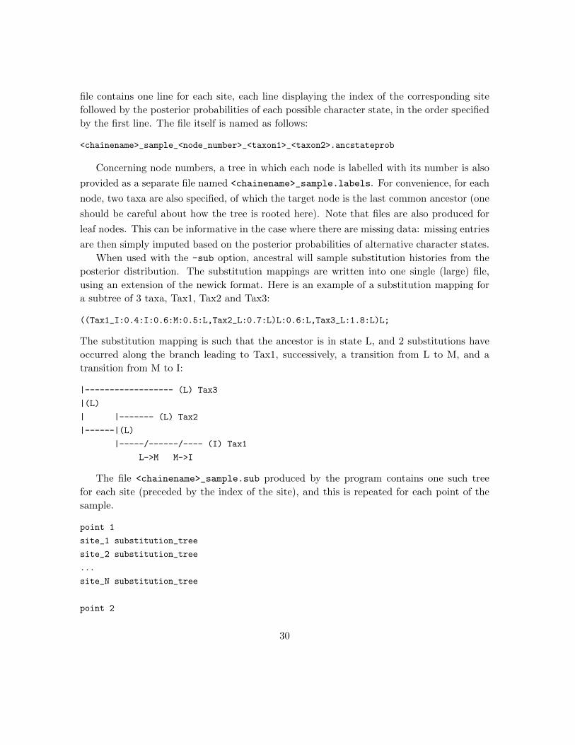
When used with the -sub option, ancestral will sample substitution histories from the
posterior distribution. The substitution mappings are written into one single (large) file,
using an extension of the newick format. Here is an example of a substitution mapping for
a subtree of 3 taxa, Tax1, Tax2 and Tax3:
((Tax1_I:0.4:I:0.6:M:0.5:L,Tax2_L:0.7:L)L:0.6:L,Tax3_L:1.8:L)L;
The substitution mapping is such that the ancestor is in state L, and 2 substitutions have
occurred along the branch leading to Tax1, successively, a transition from L to M, and a
transition from M to I:
|------------------ (L) Tax3
|(L)
| |------- (L) Tax2
|------|(L)
|-----/------/---- (I) Tax1
L->M M->I
The file <chainename>_sample.sub produced by the program contains one such tree
for each site (preceded by the index of the site), and this is repeated for each point of the
sample.
point 1
site_1 substitution_tree
site_2 substitution_tree
...
site_N substitution_tree
point 2
30
site_1 substitution_tree
site_2 substitution_tree
...
site_N substitution_tree
...
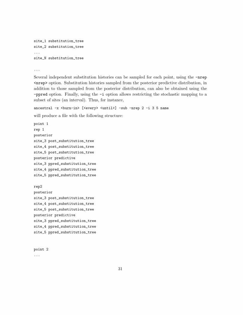
Several independent substitution histories can be sampled for each point, using the -nrep
<nrep> option. Substitution histories sampled from the posterior predictive distribution, in
addition to those sampled from the posterior distribution, can also be obtained using the
-ppred option. Finally, using the -i option allows restricting the stochastic mapping to a
subset of sites (an interval). Thus, for instance,
ancestral -x <burn-in> [<every> <until>] -sub -nrep 2 -i 3 5 name
will produce a file with the following structure:
point 1
rep 1
posterior
site_3 post_substitution_tree
site_4 post_substitution_tree
site_5 post_substitution_tree
posterior predictive
site_3 ppred_substitution_tree
site_4 ppred_substitution_tree
site_5 ppred_substitution_tree
rep2
posterior
site_3 post_substitution_tree
site_4 post_substitution_tree
site_5 post_substitution_tree
posterior predictive
site_3 ppred_substitution_tree
site_4 ppred_substitution_tree
site_5 ppred_substitution_tree
point 2
...
31
6 Cross-Validation
Cross-validation (CV) is a general method for evaluating the fit of alternative models. The
rationale is as follows: the dataset is randomly split into two (possibly unequal) parts, the
training (or learning) set and the test set. The parameters of the model are estimated on the
learning set (i.e. the model is ’trained’ on this subset of empirical observations), and these
parameter values are then used to compute the likelihood of the test set (which measures
how well the test set is ’predicted’ by the model). The overall procedure has to be repeated
(and the resulting log likelihood scores averaged) over several random splits.
Mathematically, if the original dataset D is split into D1 and D2, where D1 is the training
set used for running the chain and D2 the test set, and M is the model under which the
chain was run, then the cross-validation score is defined as:
ln p(D2 | D1,M) = ln
∫p(D2 | θ,M) p(θ | D1)dθ
where θ is the set of (global) parameters of the model. The cross-validation score is a measure
of how well the model ’predicts’ site patterns of D2 after it has ’learnt’ its parameters on
D1. This measure can be computed for alternative models Mi, i = 1..K, and models with
higher score should in principle be preferred.
Note that this measure automatically takes into account dimensionality issues and will
not intrinsically favor models that have more parameters. Intuitively, overfit means that a
model focusses to much on irrelevant (random) features of the training set. By definition,
these random features will not be consistently reproduced in the test set, and thus, an
overfitted model will typically show less good performance once evaluated on the test dataset.
Cross validation needs to be replicated (cross-validation scores typically have a large
variability, depending on the exact columns that have been included in D1 and D2). If the
original data set is D, then random pairs D1 and D2 have to be produced, by randomly
sampling columns of D (without replacement), running pb separately on each replicate of
D1, and then calculating the cross-validation score on on each resulting chain (and all this
for each model Mi). The cross-validation score can then be averaged over the replicates for
a given model. Then, supposing that a model M1 has a higher average score than M2, the
number of replicates for which the score of M1 is indeed higher than the score of M2 can be
considered as a measure of the ’significance’ of this preference for M1 over M2.
Typically, 10-fold cross-validation (such that D2 represents 10% and D1 90% of the
original dataset) has been used (e.g. Philippe et al., 2011), and ten replicates have been run
32
(although ideally, 100 replicates would certainly be more adequate). However, alternative
schemes are possible. In particular, for faster computation in the case of very large datasets,
cross-validation schemes in which the size of D1 and D2 combined together is smaller than
the size of D could be useful (as long as D1 is large enough for the parameters to be correctly
estimated).
CV is computationally intensive. However, it can be easily parallelized, as each replicated
random split can be processed independently. To achieve an optimal parallel processing, a
series of distinct programs are proposed in PhyloBayes, corresponding to each step of the
method:
• cvrep: prepare the replicates;
• pb: run each model under each replicated learning set;
• readcv: compute the cross-validation scores on each replicate;
• sumcv: pool the cv-scores and combine them into a global scoring of the models.
First, to prepare the replicated splits:
cvrep -nrep 10 -nfold 10 -d brpo.ali cvb
The number of replicates is specified with the -nrep 10 command, while -nfold 10 means
that we want to perform 10-fold cross validation: that is, for each replicate, the training
set will amount to 9/10, and the test set for 1/10, of the initial dataset. The replicates are
saved under files using the specified prefix (here, cvb):
cvb0_learn.ali, cvb0_test.ali,
cvb1_learn.ali, cvb1_test.ali,
...
Next, a MCMC is run under each learning set, and for each model, using pb. To save CPU
time, one possibility is to perform these runs under a fixed topology. Although this ignores
part of the uncertainty, for relatively large datasets, and for comparing models that usually
have large differences in their score, this should not make a big difference.
For instance, suppose we want to compare WAG and CAT:
pb -d cvb0_learn.ali -T brpo.tree -x 19 1100 CATcvb0_learn.ali
pb -d cvb0_learn.ali -T brpo.tree -x 1 1100 -wag WAGcvb0_learn.ali
33

The same should be done for the other 9 learning sets. Note that we have subsampled for the
CAT model (-x 10 11000) since this model has a more complex parameter configuration,
compared to WAG.
It is important to define the name of the chains as shown above, by prefixing the name
of the dataset with some prefix standing for the model (e.g. CATcvb0_learn.ali). This is
necessary for further processing of the resulting chains.
Once the MCMC runs have proceeded for all the replicates and all the models, the
cross-validated likelihoods are calculated using readcv:
readcv -nrep 10 -x 100 1 CAT cvb
readcv -nrep 10 -x 100 1 WAG cvb
The cross-validation score, for each replicate, is the likelihood under the test set, averaged
over the posterior distribution of the training set (see integral equation above). Here, it is ap-
proximated by averaging over the parameter values sampled by the MCMC when conditioned
on the training set, discarding a burnin of 100 points, and taking every point thereafter. The
logarithm of the resulting average is stored into a file with a .cv extension. There is one
such file for each replicate (thus, cvb0.cv, cvb1.cv, ..., cvb9.cv).
Note that, when used with the -nrep option such as above, readcv will process each
replicate successively, which may take a very long time. Alternatively readcv can be called
on individual replicates. For instance:
readcv -rep 2 -x 100 10 CAT cvb
will process only the replicate number 2. This makes it possible to split the calculation
across several processors.
Once all the cross-likelihood scores, for all the models and all the replicates, have been
obtained, they can be collected using sumcv:
sumcv -nrep 10 WAG CAT cvb
This command can be used for more than 2 models (provided that the mean cv-likelihoods
are available, and are all stored into the relevant files, with the .cv extension):
sumcv -nrep 10 WAG CAT GTR cvb
This command will average the cv-log-likelihood scores over replicates, using the first model
of the list (here WAG) as the reference.
Note that, for computational reasons, cross-validation cannot be done under the contin-
uous gamma or the Dirichlet process models of rates across sites (it works only under the
-dgam and uni models).
34

7 Priors
Branch lengths (l)
• -lexp: l ∼ iid Exponential of mean µ
• -lgam: l ∼ iid Gamma of mean µ and variance εµ2 (equivalent to the exponential
distribution when ε = 1).
• µ ∼ Exponential of mean 0.1
• ε ∼ Exponential of mean 1
Rates across sites (r)
• -cgam: r ∼ iid Gamma of mean 1 and variance 1/α
• -dgam <ncat>: r ∼ iid discretized Gamma of mean 1 and variance 1/α
• -ratecat: r ∼ Dirichlet process of granularity ζ and base distribution Gamma of
mean 1 and variance 1/α
• α ∼ Exponential of mean 1
• ζ ∼ Exponential of mean 1
Equilibrium frequency profiles across sites (π)
• -ncat 1: π ∼ Uniform
• -cat: π ∼ Dirichlet process of granularity η and base distribution G0
• -statflat: G0 = Uniform (on the simplex)
• -statfree: G0 = generalized Dirichlet, of center π0 and concentration δ
• π0 ∼ Uniform
• δ ∼ Exponential of mean S (where S is the number of states, i.e. 4 for nucleotides, 20
for amino acids)
• η ∼ Exponential of mean 10.
35

Relative exchange rates (rr)
• rr ∼ iid Exponential of mean 1
Relaxed clock; rates cross branches (ρ)
Rates across branches are relative (i.e. dimensionless). They are multiplied by a global
scaling factor, ν (expressed in number of substitutions per site and per unit of relative
time). See Lepage et al. (2007) for more details.
• -ln: ρ ∼ lognormal autocorrelated process of variance parameter σ2 (? in Thorne et
al, 1998)
• -cir: ρ ∼ CIR process of variance parameter σ2 and autocorrelation parameter θ
• -ugam: ρ ∼ iid gamma of variance parameter σ2
• ν ∼ Exponential of mean 1
• σ2 ∼ Exponential of mean 1
• θ ∼ Exponential of mean 1 with the additional constraint that θ > σ2/2 (and not
θ > σ/2 as written in Lepage et al 2007)
Divergence dates
Divergence dates are relative (dimensionless): root has divergence 1, and leaves divergence 0.
These relative dates are then multiplied by a global scale factor Scale (expressed in millions
of years) which is tuned by the -rp (root prior) option.
• -unitime: t ∼ Uniform
• -dir: t ∼ Dirichlet prior of concentration parameter χ (when χ = 1, prior is uniform).
• χ ∼ Exponential of mean 1
• -bd: t ∼ birth death process of parameters λ (birth rate), µ (death rate) and ω
(sampling fraction). To ensure identifiability, we set p1 = λ− µ and p2 = λω.
• p1 ∼ Exponential of mean 1
• p2 ∼ Exponential of mean 1
36
• Scale ∼ Uniform by default. this is an improper prior. Override if possible.
• -rp <mean> <stdev>: Scale ∼ Gamma of specified mean and standard deviation.
Covarion model
The covarion parameters can be expressed as
• s01 = ξ(1− p0): rate from OFF to ON
• s10 = ξp0: rate from ON to OFF
where ξ is the rate of the ON-OFF process, and p0 the stationary probability of the OFF
state.
• ξ ∼ Exponential of mean 1
• p0 ∼ Uniform over [0, 1]
37
References
Bollback, Jonathan P. 2002. Bayesian model adequacy and choice in phylogenetics. Mol.
Biol. Evol. 19:1171–1180.
Delsuc, Frederic, Georgia Tsagkogeorga, Nicolas Lartillot, and Herve Philippe. 2008. Addi-
tional molecular support for the new chordate phylogeny. Genesis 46:592–604.
Douzery, Emmanuel, Elizabeth Snell, Eric Bapteste, Frederic Delsuc, and Herve Philippe.
2004. The timing of eukaryotic evolution: does a relaxed molecular clock reconcile proteins
and fossils? Proc. Natl. Acad. Sci. USA 101:15386–15391.
Drummond, Alexei, Simon Ho, Matthew Phillips, and Andrew Rambaut. 2006. Relaxed
phylogenetics and dating with confidence. PLoS Biol. 4:e88.
Ferguson, T S. 1973. A Bayesian analysis of some nonparametric problems. Ann. Statist.
209–230.
Gelman, Andrew, John B Carlin, Hal S Stern, and Donald B Rubin. 2004. Bayesian Data
Analysis. Chapman & Hall/CRC.
Geyer, C. 1992. Practical Markov Chain Monte Carlo. Stat. Sci. 7:473–483.
Huelsenbeck, John P., and Marc A. Suchard. 2007. A nonparametric method for accommo-
dating and testing across-site rate variation. Syst. Biol. 56:975–987.
Inoue, Jun, Philip C J Donoghue, and Ziheng Yang. 2010. The impact of the representation
of fossil calibrations on Bayesian estimation of species divergence times. Syst. Biol. 59:74–
89.
Kishino, H, J Thorne, and W Bruno. 2001. Performance of a divergence time estimation
method under a probabilistic model of rate evolution. Mol. Biol. Evol. 18:352–361.
Kolaczkowski, Bryan, and Joseph W Thornton. 2008. A mixed branch length model of
heterotachy improves phylogenetic accuracy. Mol. Biol. Evol. 25:1054–1066.
Lartillot, Nicolas, Henner Brinkmann, and Herve Philippe. 2007. Suppression of long-branch
attraction artefacts in the animal phylogeny using a site-heterogeneous model. BMC Evol.
Biol. 7 Suppl 1:S4.
38
Lartillot, Nicolas, and Herve Philippe. 2004. A Bayesian mixture model for across-site
heterogeneities in the amino-acid replacement process. Mol. Biol. Evol. 21:1095–1109.
Le, Si Quang, and Olivier Gascuel. 2008. An improved general amino acid replacement
matrix. Mol. Biol. Evol. 25:1307–1320.
Le, Si Quang, Nicolas Lartillot, and Olivier Gascuel. 2008. Phylogenetic mixture models for
proteins. Philos. Trans. R. Soc. Lond. B Biol. Sci. 363:3965–3976.
Lepage, Thomas, David Bryant, Herve Philippe, and Nicolas Lartillot. 2007. A general
comparison of relaxed molecular clock models. Mol. Biol. Evol. 24:2669–2680.
Lewis, Paul O. 2001. A Likelihood Approach to Estimating Phylogeny from Discrete Mor-
phological Character Data. Syst. Biol. 50:913–925.
Meng, Xiao-Li. 1994. Posterior predictive p-values. Ann. Statist. 1142–1160.
Nielsen, Rasmus. 2002. Mapping mutations on phylogenies. Syst. Biol. 51:729–739.
Philippe, Herve, Henner Brinkmann, Richard R Copley, Leonid L Moroz, Hiroaki Nakano,
Albert J Poustka, Andreas Wallberg, Kevin J Peterson, and Maximilian J Telford. 2011.
Acoelomorph flatworms are deuterostomes related to Xenoturbella. Nature 470:255–258.
Quang, Le Si, Olivier Gascuel, and Nicolas Lartillot. 2008. Empirical profile mixture models
for phylogenetic reconstruction. Bioinformatics 24:2317–2323.
Thorne, J L, H Kishino, and I S Painter. 1998. Estimating the rate of evolution of the rate
of molecular evolution. Mol. Biol. Evol. 15:1647–1657.
Tuffley, C, and M Steel. 1998. Modeling the covarion hypothesis of nucleotide substitution.
Math Biosci 147:63–91.
Wang, Huai-Chun, Karen Li, Edward Susko, and Andrew J Roger. 2008. A class frequency
mixture model that adjusts for site-specific amino acid frequencies and improves inference
of protein phylogeny. BMC Evol. Biol. 8:331.
Yang, Z. 1994. Maximum likelihood phylogenetic estimation from DNA sequences with
variable rates over sites: approximate methods. J. Mol. Evol. 39:306–314.
39

Yang, Ziheng, and B Rannala. 2006. Bayesian estimation of species divergence times under
a molecular clock using multiple fossil calibrations with soft bounds. Mol. Biol. Evol.
23:212–226.
Zhou, Yan, Nicolas Rodrigue, Nicolas Lartillot, and Herve Philippe. 2007. Evaluation of the
models handling heterotachy in phylogenetic inference. BMC Evol. Biol. 7:206.
40