This paper presents preliminary findings and is being distributed to economists and other interested readers solely to stimulate discussion and elicit comments. The views expressed in this paper are those of the authors and are not necessarily reflective of views at the Federal Reserve Bank of New York or the Federal Reserve System. Any errors or omissions are the responsibility of the authors.

Federal Reserve Bank of New York Staff Reports

A Bargaining Theory of Trade Invoicing and Pricing

Linda Goldberg Cédric Tille

Staff Report No. 611 April 2013

A Bargaining Theory of Trade Invoicing and Pricing Linda Goldberg and Cédric Tille Federal Reserve Bank of New York Staff Reports, no. 611 April 2013 JEL classification: F30, F40

Abstract We develop a theoretical model of international trade pricing in which individual exporters and importers bargain over the transaction price and exposure to exchange rate fluctuations. We find that the choice of price and invoicing currency reflects the full market structure, including the extent of fragmentation and the degree of heterogeneity across importers and across exporters. Our study shows that a party has a higher effective bargaining weight when it is large or more risk tolerant. A higher effective bargaining weight of importers relative to exporters in turn translates into lower import prices and greater exchange rate pass-through into import prices. We show the range of price and invoicing outcomes that arise under alternative market structures. Such structures matter not only for the outcome of specific exporter-importer transactions, but also for aggregate variables such as the average price, the average choice of invoicing currency, and the correlation between invoicing currency and the size of trade transactions. Key words: currency, invoicing, exchange rate _________________

Goldberg: Federal Reserve Bank of New York (e-mail: linda.goldberg@ny.frb.org). Tille: Graduate Institute of International and Development Studies, Geneva (e-mail: cedric.tille@graduateinstitute.ch). The authors thank Charles-Henry Weymuller and seminar participants at the Federal Reserve Bank of New York, the HEID-EPFL-UNIL Sinergia workshop, the Bank of Italy, the National Bank of Serbia, the University of Reading, the University of Navarra, and the University of Basel for valuable comments. The views expressed in this paper are those of the authors and do not necessarily reflect the position of the Federal Reserve Bank of New York or the Federal Reserve System.

1 Introduction

What determines the currency used in the invoicing of international trade?

This question is the subject of an extensive theoretical and empirical research

agenda in international economics as it plays a central role in determining whom

among exporters or importers bear the cost of exchange rate fluctuations, and

whether these fluctuations affect trade quantities. The existing theoretical liter-

ature has identified a host of determinants of the choice of invoicing currency in

international trade, including a "coalescing" motive for exporters to keep their

prices close to their competitors’, a "hedging" motive to movements in marginal

revenue in line with marginal cost fluctuations, transaction costs in foreign ex-

change markets, and the role of macroeconomic conditions that favor the use of

low volatility currencies.1

A limit of existing contributions is the assumption that the choice of the invoic-

ing currency rests solely with the exporter, who takes into account the downward

sloping demand of importers. This assumption of unilateral decision-making is

however at odds with growing evidence that the invoicing choice reflects a bar-

gaining between exporters and importers (see Friberg and Wilander 2008 and Ito

et al. 2012).

This paper addresses this limit by developing a richer model of the interac-

tion between exporters and importers. We develop a simple model of bargaining

between individual exporters and importers, with each taking into account the

outside option of her counterpart. The negotiating covers both the allocation of

exchange rate risk through the choice of invoicing currency and the price level in

that currency.2

1Aggregate macroeconomic conditions impoly choosing a currency with low transaction costs

(Devereux and Shi 2005 and Portes and Rey 2001), low macroeconomic volatility (Devereux,

Engel, and Storgaard 2004), and hedging benefits which take into account the use of imported

inputs (Novy 2006). The role of exporter market share is emphasized (Bacchetta and van

Wincoop 2005, and Auer and Schoenle 2012), as is coalescing across his competitors contingent on

demand elasticities and production curvature (Goldberg and Tille 2008). Endogenous currency

choice also arises in a framework of uncertain timing of future price resets (Gopinath, Itskhoki,

and Rigobon 2010).2Recent works that focus on strategic interactions across competing exporting firms, but

1

In our model a range of exporters produce goods at a cost and sell them to

a range of importers, who in turn resell these goods in their domestic market.

Each exporter - importer pair bargains over the two aspects of the contract: a

preset contract price that prevails in the absence of exchange rate movements

between the time of contracting and the time of the actual transaction, and the

allocation of exposure to exchange rate movements around that preset price (i.e.

the invoicing currency), which maps directly to rates of ex-post exchange rate

pass through. We consider a standard Nash bargaining that maximizes a joint

surplus which is a weighted average of the exporter’s and importer’s surpluses,

with the weights referred to as the formal bargaining weights of the parties.3 As all

exporters transact with all importers in equilibrium, the surplus that an exporter

gets from a successful match with a specific importer is the utility of the profits

from transacting with all importers minus the utility of the profits from transacting

with all importers except the specific importer in the bargaining. The surplus for

an importer is defined similarly.

Our analysis includes three key ingredients. First, exporters and importers

have a concave valuation of payoffs. Failing to reach an agreement with a large

counterpart then has a larger impact on the marginal valuation of payoffs than

failing to reach one with a small counterpart. Second, uncertainty plays a central

role as the bargaining takes place before exchange rate fluctuations are realized.

Third, we allow for heterogeneity of exporters and importers, with heterogeneity

taking the form of numbers of counterparts or relative sizes of counterparts. To our

knowledge this paper is the first analysis of the joint determination of pricing and

invoicing through a bargaining in the presence of uncertainty and heterogenous

valuations of payoffs.

The key relations in our analysis are the first-order conditions that maximize

the joint surplus of a specific exporter - importer pair with respect to the preset

price and the exchange rate exposure. Two conditions are derived for each exporter

- importer pair. As they are highly non-linear, we first solve for the optimal

prices in a steady-state with no uncertainty. We then solve for the exchange rate

exposure by relying on a quadratic approximation around the steady-state, such an

approximation being needed to capture the second moments that drive the choice

without a focus on the importer competition or bargaining, include deBlas and Russ (2012) and

Garetto (2012).3The weights are the same across all exporter - importer pairs.

2

of exposure. In general the preset price and exposure choice for a specific exporter

- importer pair depends on the choices for other pairs, as these affect the marginal

value of payoffs for the parties. As this leads to a highly complex solution, we

consider two specific cases to highlight the key results. The first case focuses on

the degree of fragmentation among exporters and among importers, defined as the

number of identical agents in each group. The second case emphasizes intra-group

heterogeneity, defined as the relative size of agents within each group, setting the

number of agents per group to two.

The analysis leads to a number of novel results. First, the outcomes of the

bargaining reflects the effective bargaining weights of the counterparts that differ

from the formal weights in the joint surplus. A counterpart gets a higher effective

bargaining weight when she is big and when the concavity of her valuation of payoffs

is limited. The size of a counterpart is measured by the share of her counterpart’s

payoffs that she accounts for in equilibrium.4 Second, the preset price is tilted

in favor of the counterpart with the highest effective bargaining weight. This

party then gets most of the surplus from the match, but also has a lower marginal

value of payoffs relative to the other party due to the concavity of valuation of

payoffs. Third, the counterpart with the highest effective bargaining weight bears

more of the exchange rate risk. This result is both interesting and intuitive. This

counterpart has a relatively low marginal value of payoffs, which implies that ex-

post movements have a relatively limited impact on marginal utility. These results

also underscore the importance of considering a bargaining process that covers all

aspects of the price contract, and not just the exchange rate exposure. Fourth,

in the presence of intra-group heterogeneity, the relative sizes of agents within

each group affect the outcome not only for specific pairs but also in aggregate

terms. Specifically, a situation of high exporter heterogeneity (with one exporter

dominating the market) is characterized by a higher average level of preset prices

across pairs, a higher average exposure of exporters to exchange rate movements

(more importer currency pricing), and a positive correlation between the value of

transactions and the exchange rate exposure of exporters.

In addition to its contribution to our understanding of the determinants of in-

ternational trade invoicing and price-setting, this paper provides a methodological

contribution by solving a bargaining model under uncertainty where the marginal

4For instance the exporter’s size in a specific exporter - importer pair is the share of the

importer’s profits that stems from buying and selling the goods produced by the exporter.

3

valuations of payoffs differs across the parties. As outlined in the discussion of

the related literature, existing contributions consider some of the aspects of our

framework (such as uncertainty or different valuations of payoffs), but our analysis

is to our knowledge the first that encompasses the combined features.

The paper is organized as follows. We review the related literature on pricing

and invoicing currency choice, as well as on bargaining games, in Section 2. Sec-

tion 3 presents the main features of the model, and Section 4 provides the solution

method. Sections 5 derives the outcomes for preset prices and exchange rate expo-

sure in specific examples, focusing first on fragmentation and then on intra-group

heterogeneity among exporters and importers. Section 6 concludes. Throughout

the paper we focus on an intuitive presentation of the main points. The key tech-

nical aspects are presented in the Appendix and the detailed derivations are in a

Technical Appendix available on request.

2 Related literature

Our work fits in the literature on invoicing choice and price adjustments in inter-

national economics, providing additional theoretical underpinnings on the roles of

firm and industry-level heterogeneity that are found to be important in empiri-

cal studies. Goldberg and Tille (2011) consider a highly disaggregated data set

of Canadian imports and find a robust link between invoice currency choice, the

size of individual transactions, and heterogeneity of transacting agents. Berman,

Martin, and Mayer (2012) analyze rich data for French firms and find that high

performance firms have markups that respond more to exchange rate movements,

and are more willing to engage in producer currency pricing.5 Gopinath, Itskhoki,

and Rigobon (2010) show that invoice currency choice is closely related to the

pass-through of cost fluctuations into final prices in the United States, with much

higher pass-through for import prices set in currencies other than the dollar. Price

rigidities do not fully explain this phenomenon. 6

5For these firms, quantities of high performance firms also respond by less to exchange rate

changes. Sectoral heterogeneity in pricing also varies according to types of goods, with more

local currency pricing on consumer goods than intermediate goods, and more for sectors with

higher distribution costs.6As our model assumes that prices are fully preset, up to the exchange rate exposure, we

cannot consider the relation between the choice of invoicing and the response of prices to cost

4

Our paper also relates to the industrial organization literature on bargain-

ing games between suppliers and retailers. To our knowledge, our paper is the

first contribution introducing bargaining between buyers (exporters) and sellers

(importers) in the context of concave valuation of payoffs in an uncertain environ-

ment. The nearest contributions include DeGraba (2005), who presents a model

where the valuation of goods varies across buyers. Sellers make price offers that

the buyers can accept or refuse. As the seller cannot observe the true valuation

of her counterpart, she has an incentive to offer better conditions to larger buyers

as loosing a large customer is more costly than loosing a larger one. While the

DeGraba model includes uncertainty, it does so in the form of idiosyncratic valu-

ations and thus abstracts from the role of aggregate risk such as that arising from

exchange rate movements. The role of curvature in valuation, which we assume,

has a precedent in the framework of Normann et al. (2003) wherein a seller with

increasing marginal costs of production makes take it or leave it offers to buyers.

The seller offers a lower price to large buyers as large sales take place at a point

on the curve schedule where the marginal cost his low. The setting however does

not include uncertainty.

A number of other papers provide theoretical precedent for our treatment of

counterpart heterogeneity and fragmentation through their focus on merger incen-

tives in multi-agents games. Inderst and Wey (2003) develop a framework where

prices are set between two retailers and two producers, but assume that all agents

share the same marginal valuation of resources in contrast to our setting of het-

erogenous concave valuations.7 Horn and Wolinsky (1988) analyze a setting with

two buyers and two sellers where the marginal valuation of the price can differ be-

tween buyers and sellers, and focus on the incentives of agents to merge and form

a monopoly, showing that this is not necessarily an optimal choice because of the

impact on bargaining power. The model, however, assumes that each buyer only

purchases from one seller, and thus abstracts from the ability of buyers to play one

seller against another to gain a better bargaining position. Dowbson and Waterson

(1997) consider a larger number of identical buyers, but abstract from uncertainty

fluctuations. Our assumption is motivated by our focus on invoicing in a novel pricing framework,

and extending it to include price adjustment is left for future work. The relevance of market

structure for invoicing is likely to extend to price adjustment as well.7Similarly, Chipty and Snyder (1999) focus on the incentives for mergers among buyers and

sellers assuming that they share the same marginal valuation of the price.

5

and heterogeneity in payoffs’valuation. Camera and Selcuk (2009) show how price

heterogeneity can arise in a setting with homogenous buyers and homogenous sell-

ers, but abstract from uncertainty. This follows from capacity constraints faced by

sellers, while the heterogeneity in our model reflect different sizes of agents. Selcuk

(2012) introduces risk averse differences between buyers and sellers. A seller faced

with risk-averse buyers opts to set a fixed price so that buyers are not exposed

to ex-post price risk. In his setting the price, the risk facing the buyer is due to

limited sellers’inventories, instead of the macroeconomic risk that we consider. In

addition, risk aversion is limited to one side of the market.

Overall, our setting differs from the existing theoretical contributions in the in-

dustrial organization literature in that we consider aggregate uncertainty, heteroge-

nous marginal valuation of payoffs through concave valuations, and heterogeneity

in terms of agents sizes.

3 An exporter-importer bargaining model

3.1 Structure and payoffs

Two types of agents are in the model: importers and exporters. There are M

importers indexed by j, and X exporters indexed by i. Exporters sell goods to

importers, who in turn resell these goods to customers in the destination country.

A specific importer m buys Qxm units of goods from a specific exporter x and

resells these goods at a price Zm in her currency. Exporter x has an average

production cost denoted by Cxm and denominated in her currency. Each importer

can purchase goods from all exporters, and each exporter can sell goods to all

importers. When transactions occur for all exporter-importer pairs (which is the

case in equilibrium) the payoffof importerm is a concave valuation of her expected

profits:

Um =1

1− γME

(X∑i=1

(Zm − Pmim)Qim

)1−γM

(1)

where E is the expectation operator, γM captures the concavity of the importer’s

valuation of payoffs (and her risk aversion) that is common to all importers, and

Pmim is the price charged by exporter i to importer m, with the m superscript

denoting that this price is expressed in the importer’s currency. The payoff of

6

exporter x is a concave valuation of her expected profits:

Ux =1

1− γXE

(M∑j=1

(P xxj − Cxj

)Qxj

)1−γX

(2)

where γX captures the concavity of the exporter’s valuation of payoffs (common

to all exporters), and P xxj is the price charged by exporter x to importer j, with

the x subscript denoting that it is expressed in the exporter’s currency. The

specifications (1)-(2) encompass two key features of the model, namely the presence

of uncertainty with the valuation of payoffs being from an ex-ante perspective, and

the concave valuation of payoffs reflected by the constant relative risk aversion

paramaters, γM and γX , that can differ between exporters and importers.

Our analysis focuses on the price charged by exporter x to importer m. It

entails two contractual components: a preset price component P fxm that is fixed

before shocks are realized, and the extent to which the price in the importer’s

currency moves with ex-post fluctuations in the exchange rate. Specifically, we

denote the percentage of exchange rate movements that are transmitted to the

importer’s price by 1 − βxm, where βxm ∈ (0, 1). We interpret βxm as the extent

of local currency pricing (LCP), which corresponds to the share of exchange rate

movements that are absorbed by the exporter. If βxm = 1 the importer is shielded

from exchange rate fluctuations, corresponding to full local currency pricing. If

βxm = 0 the exporter’s price is shielded from exchange rate fluctuations, a case

referred to as producer currency pricing (PCP) in the literature.8 The exchange rate

S is defined as units of exporter’s currency per unit of importer’s currency, so that

an increase corresponds to a depreciation of the exporter’s currency. We assume,

without loss of generality, that the log exchange rate s is normally distributed

around zero.

The price paid by the importer in her currency is:

Pmxm = P f

xmSβxm−1

Similarly the price received by the exporter in her currency is:

P xxm = P b

xmS = P fxmS

βxm

8Engel (2006) and Goldberg and Tille (2008) provide equivalence results on optimal exchange

rate pass through and invoice currency choice when prices are sticky.

7

The price between exporter x and importer m is determined through bilateral

bargaining. A key element is the surplus that each counterpart gains from a

successful match (defined as a negotiation that leads the pair xm to undertake a

transaction). In equilibrium there are transactions between all importer-exporter

pairs, as all transactions generate some positive surplus making both exporter

and importer better off by transacting. The surplus of the importer (exporter)

specifically generated by the xm transaction is the value of the payoff for the

importer (exporter) from conducting transactions with all counterparts, minus the

payoff she would get from conducting transactions with all counterparts except x

(m).9

Specifically, the expected surplus that importer m derives from its negotiation

with exporter x is:

Θmxm =

1

1− γME

(X∑i=1

(Zm − P f

imSβxm−1

)Qim

)1−γM

(3)

− 1

1− γME

( ∑Xi=1

(Zm − P f

imSβxm−1

)Qim

−(Zm − P f

xmSβxm)Qxm

)1−γM

Similarly the surplus for x from its negotiation with importer m is:

Θxxb =

1

1− γXE

(M∑j=1

(P fxjS

βxj − Cxj)Qxj

)1−γX

(4)

− 1

1− γXE

( ∑Mj=1

(P fxjS

βxj − Cxj)Qxj

−(P fxmS

βxm − Cxm)Qxm

)1−γX

We allow for the quantity Qxm to be price sensitive. Specifically, the demand

by m for goods produced by x is inversely related to the ratio between the price

Pmxm charged by x to m, and a reference price denoted by R

mxm which reflects the

prices that m gets from other competing exporters. We consider a constant price

elasticity of demand ρ. The reference price Rmxm is of a form similar to the price

Pmxm, and consists of a fixed component R

m,fxm and a component that is sensitive

to the exchange rate: Rmxm = Rm,f

xm Sηxm−1, where ηxm is the extent to which the

9The structure is similar to Chipty and Snyder (1999) where an individual buyer negotiates

with the seller assuming that the seller will trade with all other buyers, so that each buyer views

himself as being the marginal buyer.

8

reference price is stable in the importer’s currency. A more detailed presentation

of the reference price is provided in the numerical examples of sections 4 and 5.

The quantity sold from x to m is then written as:

Qxm = Qsetxm

[P fxm

Rm,fxm

S(βxm−ηxm)

]−ρ(5)

where Qsetxm is the exogenous component of demand, which is not affected by the

outcome of the price and invoice currency bargaining.

The quantity Qxm is produced according to a decreasing returns to scale tech-

nology which uses an input Lxm. We assume that the technology, and hence the

average and marginal costs, apply separately to each xm pair.10 Specifically the

technology is Qxm = Axm (Lxm)λ where Axm is a constant parameter and λ ≤ 1.

For simplicity, we assume that the production by exporter x of the goods she sells

to m is not affected by the quantities she sells to other importers, and so are the

average cost Cxm and the marginal costMCxm = λ−1Cxm.11 We allow for the unit

cost of the input to be affected by the exchange rate, for example due to the use

of imported inputs in production, and denote the unit cost by WxSζx where Wx

is exogenous and ζx is the elasticity of the cost with respect to the exchange rate.

Under this specification the marginal cost of production is:

MCxm =1

λWxS

ζx (Axm)−1λ

[Qsetxm

[P fxm

Rm,fxm

S(βxm−ηxm)

]−ρ] 1−λλ

(6)

We consider a partial equilibrium setting in order to focus on the interaction

between the respective exporters and importers. In particular, we take several

variables to be exogenous, such as the exchange rate S, the final price Zm, the

wage Wx, the reference price Rmxm, and the demand shifter Q

setxm. We consider that

these variables are stochastic, and possibly correlated.

3.2 Determination of price

The two components of the contract negotiated between x and m, namely the

preset contract price pfxm and the extent of invoicing in the importer’s currency10Accordingly, there is no spillover of the outcome between a specific importer-exporter pair

and the costs for another transacting pair.11This can be interpreted as x operating a plant producing only for sales to m. If instead we

assume that the plant produces for all of x’s customers, sales to importers other than m would

affect the marginal cost of selling to m.

9

βxm, are set to maximize a combination of the exporter’s and importer’s surpluses

(3) and (4). We consider a Nash bargaining where the combination is a geometric

averages of the surpluses, with weights representing the formal bargaining weights

of the parties. This approach is standard in the bargaining literature, as in Chipty

and Snyder (1999), Dowbson andWaterson (1997), and Horn andWolinsky (1988).

Specifically we define the joint surplus of a match between x and m as:

Θjointxm = [Θm

xm]δ [Θxxm]1−δ (7)

where δ captures the formal weight of the importer in the bargaining, and is

assumed to be the same for all xm pairs. It reflects the role that the importer

plays in determining the price and invoicing. The cases of δ = 0 is the situation

where the exporter makes the decision unilaterally to maximize her surplus given

her knowledge of all the relevant parameters of demand. Similarly, the importer

is the sole decider when δ = 1. Each party has an equal say when δ = 0.5. The

assumption that the two parties have identical weights (i.e δ = 0.5) is standard in

the literature (Chipty and Snyder 1999, Dowbson and Waterson 1997, and Horn

and Wolinsky 1988)

The preset contract price P fxm and extent of LCP βxm are chosen to maximize

(7) leading to the two following conditions:

0 = δ∂Θm

xm

∂P fxm

Θxxm + (1− δ) ∂Θx

xm

∂P fxm

Θmxm (8)

0 = δ∂Θm

xm

∂βxmΘxxm + (1− δ) ∂Θx

xm

∂βxmΘmxm (9)

The exact expression of the various derivatives in (8) and (9) are complex and

given in the appendix.12

12Our framework differs significantly from, and complements, that of Gopinath, Itskhoki and

Rigobon (2010). Our model focuses on the interaction between heterogeneous exporters and

importers. We abstract from dynamics by considering an ex-ante stage with the negotiation over

the terms of a contract that yields the relevant decisions on ex ante pricing and allocation of

exchange rate risk, and an ex-post stage where shocks are realized and exchange rate movements

are transmitted to prices according to the agreed exposure. Unlike the multiperiod framework

of Gopinath, Itskhoki and Rigobon (2010), we do not consider staggered and uncertain timing

of pricing adjustments, and thus cannot discuss the connection between exchange rate exposure

and pass-through at the time when prices are adjusted, which is central in their analysis.

10

4 Solution method

4.1 Steady state

The first-order conditions (8) and (9) are non-linear functions of the pricing

components not only between x andm, but also between x and the other importers,

as well as between m and the other exporters. This reflects the fact that the

surpluses (3)-(4) are affected by all of the exporter-importer transactions.

As there is no closed-form solution of the system (8) and (9), we consider

approximations around a steady state where there is no uncertainty. We denote

steady-state variables with an upper bar. Without loss of generality we assume

that the exchange rate is equal to unity: S = 1. The price in any currency then

corresponds to its preset component (Pmxm = P x

xm = P fxm) which we denote by Pxm

for brevity.

A convenient way to capture the relevance of importer m for exporter x is to

compute the share of x’s total profits that are accounted for by sales to m:

Πmxm =

(Pxm − Cxm

)Qxm∑M

j=1

(Pxj − Cxj

)Qxj

(10)

with a high value of Πmxm indicating that the importer m is large from the point of

view of the exporter x. Similarly the relevance of exporter x for importer m is the

share of m’s profits that come from sales of goods provided by x:

Πxxm =

(Zm − Pxm

)Qxm∑X

i=1

(Zm − Pim

)Qim

(11)

with a high value of Πxxm indicating that the exporter x is large from the point of

view of the importer m.

The invoicing share βxm does not enter the steady-state solution.13 Intuitively,

it is not a meaningful dimension of the model in the absence of exchange rate

fluctuations.14 We therefore focus on the steady state value of (8) which is:

δxm

(Pxm −

ρ

ρ− 1Zm

)(Pxm − Cxm

)=

(1− δxm

)(Pxm −

ρ

ρ− 1MCxm

)(Zm − Pxm

)(12)

13Specifically, both sides of (9) are zero when evaluated at the steady state.14A parallel intuition arises in the context of the allocation of wealth into a portfolio of various

assets. If all assets yield the same return with certainty, investors are indifferent across portfolios.

11

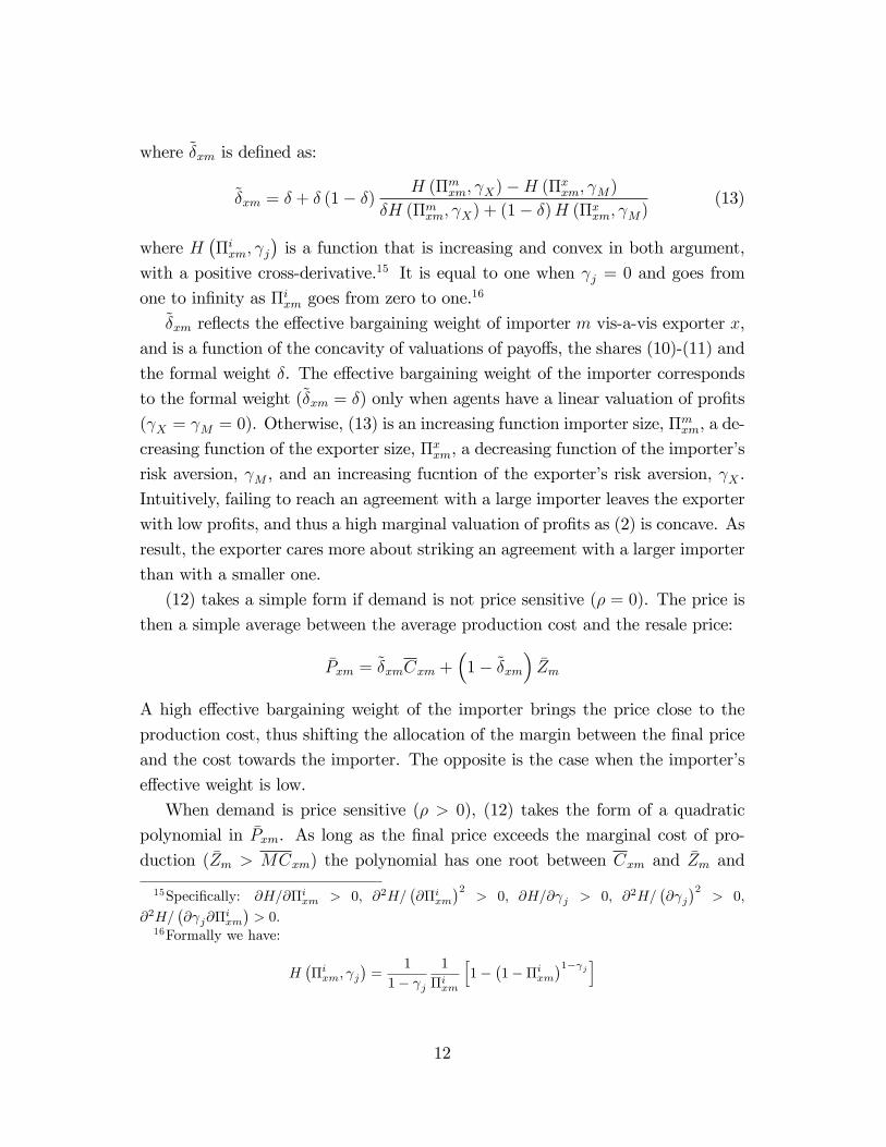
where δxm is defined as:

δxm = δ + δ (1− δ) H (Πmxm, γX)−H (Πx

xm, γM)

δH (Πmxm, γX) + (1− δ)H (Πx

xm, γM)(13)

where H(Πixm, γj

)is a function that is increasing and convex in both argument,

with a positive cross-derivative.15 It is equal to one when γj = 0 and goes from

one to infinity as Πixm goes from zero to one.16

δxm reflects the effective bargaining weight of importer m vis-a-vis exporter x,

and is a function of the concavity of valuations of payoffs, the shares (10)-(11) and

the formal weight δ. The effective bargaining weight of the importer corresponds

to the formal weight (δxm = δ) only when agents have a linear valuation of profits

(γX = γM = 0). Otherwise, (13) is an increasing function importer size, Πmxm, a de-

creasing function of the exporter size, Πxxm, a decreasing function of the importer’s

risk aversion, γM , and an increasing fucntion of the exporter’s risk aversion, γX .

Intuitively, failing to reach an agreement with a large importer leaves the exporter

with low profits, and thus a high marginal valuation of profits as (2) is concave. As

result, the exporter cares more about striking an agreement with a larger importer

than with a smaller one.

(12) takes a simple form if demand is not price sensitive (ρ = 0). The price is

then a simple average between the average production cost and the resale price:

Pxm = δxmCxm +(

1− δxm)Zm

A high effective bargaining weight of the importer brings the price close to the

production cost, thus shifting the allocation of the margin between the final price

and the cost towards the importer. The opposite is the case when the importer’s

effective weight is low.

When demand is price sensitive (ρ > 0), (12) takes the form of a quadratic

polynomial in Pxm. As long as the final price exceeds the marginal cost of pro-

duction (Zm > MCxm) the polynomial has one root between Cxm and Zm and

15Specifically: ∂H/∂Πixm > 0, ∂2H/

(∂Πi

xm

)2> 0, ∂H/∂γj > 0, ∂2H/

(∂γj)2

> 0,

∂2H/(∂γj∂Πi

xm

)> 0.

16Formally we have:

H(Πixm, γj

)=

1

1− γj1

Πixm

[1−

(1−Πi

xm

)1−γj]

12

another above Zm. We rule out the second root as it implies that the importer

makes negative profits (Pxm > Zm). The first root by contrast implies that both

the exporter and the importer make positive profits (Pxm > Cxm and Zm > Pxm).

Our analysis shows that the steady state solution is a fixed point characterized

by the shares of the exporter (importer) in their counterpart’s payoff, (10)-(11),

which are functions of the prices between them, and by the price (12) which is a

function of the shares (10)-(11) through the effective bargaining weight (13). The

steady-state solution is the fixed point of these relations. While we cannot derive

an analytical solution for this fixed point in general, we can compute the solution

for specific cases presented in section 5.17

4.2 Approximation around the steady state

The next step of the solution method is to expand the first-order conditions

(8) and (9) around the steady-state. Our analysis requires us to consider quadratic

log approximations for two reasons. First, the extent of LCP βxm determines who

bears the exchange rate risk outside of the steady state. Computing βxm then

requires that we include the second moments of the equations through a quadratic

approximation. Second, the preset component of the price, P fxm, differs from the

steady state price Pxm in (12) in the presence of risk, as forward-looking agents

take account of the second moments when setting the price.18 Specifically, the

preset component of the price can be written as P fxm = Pxm exp [%σ2] where % is a

coeffi cient and σ2 is proportional to the variances of the (log of the) shocks to the

exchange rate, final prices, wages, and demand shifters. We denote the logarithms

of the various variables by lower case letters.

As shown below, the extent of LCP βxm is computed using the quadratic ap-

proximation of (9) across all xm pairs. The log of preset prices pfxm can then be

computed from the quadratic approximation of (8). In our analysis we focus on

the first step and abstract from the second step for two reasons. First, solving

17The presence of decreasing returns to scale (λ < 1) implies that the size of the exogenous

output for the xm pair, Qsetxm in (5), affects the marginal and average costs for the pair, making

the analysis more complex. In the remainder of our analysis, we shut this dimension down by

appropriately scaling the productivity Axm to(Qsetxm

)1−λ, so that Qsetxm and Axm offset each other

in the steady state marginal cost (6).18This element is a standard feature in the analysis of optimal monetary policy in models

where prices are set ex-ante by forward looking agents.

13

for the invoicing shares does not require knowing the price gap between pfxm and

ln(Pxm

). Second, the gap is of the form %σ2 and can thus be set to be arbitrarily

small by choosing a small variance of shocks. By contrast, the invoicing shares

βxm are independent from the volatility of shocks (as long as this volatility is not

zero).19

We expand (9) around the steady state with respect to the logs of the pre-

set component of the price pfxm, the exogenous exchange rate s, the exogenous

component of the input cost wx, the exogenous final price zm, and the exogenous

component of demand qsetxm.20 We denote logs deviation from the steady state with

hatted values: zm = zm − ln[Zm].

The quadratic approximation of (9) leads to the following expression (the steps

are presented in the appendix):

0 = − ρZmρZm + (1− ρ) Pxm

Ezms

Es2+

ρMCxm

(1− ρ) Pxm + ρMCxm

(Ewxs

Es2+ ζx

)+

ρMCxm

(1− ρ) Pxm + ρMCxm

1− λλ

(Eqsetxms

Es2− ρ (βxm − ηxm)

)(14)

+(1− ρ) Pxm

ρZm + (1− ρ) Pxm(1− βxm) +

(1− ρ) Pxm

(1− ρ) Pxm + ρMCxm

βxm

+γM

[X∑i=1

Πiim

(Zm

Zm−PimEzmsEs2

+ PimZm−Pim (1− βim)

+Eqsetim s

Es2− ρ (βim − ηim)

)]

−γX

M∑j=1

Πjxj

PxjPxj−Cxj

βxj −Cxj

Pxj−Cxj

(EwxsEs2

+ ζx)

+Pxj−MCxjPxj−Cxj

(Eqsetxj s

Es2− ρ

(βxj − ηxj

))

The first three rows of (14) reflect various aspects for the xm pair that affect

the optimal LCP. The first driver is the comovement between the final price and

the exchange rate, (Ezms) (Es2)−1. If the final price moves in step with the ex-

change rate, the importer is willing to accept lower LCP. The intuition is that

the importer can sell the goods at a higher final price when a depreciation of her

currency raises the price she pays in her currency for imports. The second driver

19In technical terms, βxm is similar to a portfolio share in models of endogenous portolfio

choice such as Tille and van Wincoop (2010). Such so-called "zero-order" shares depend not on

the magnitude of volatility (as long as it is positive) but on the co-movements between asset

returns and pricing kernels.20The deviation of the price pfxm from the steady state being proportional to the variance of

shocks (i.e. "second order") it ends up dropping out of the approximation.

14

is the comovement between the exporter’s production cost and the exchange rate,

either directly through importer input costs ζx or indirectly through comovements

between wages and the exchange rate, (Ewxs) (Es2)−1. If production costs in-

crease when the importer’s currency weakens, the exporter is less willing to accept

high LCP. The third driver is the impact of exchange rate movements on demand

either through different degrees of LCP relative to competitors, βxm − ηxm, whichaffects demand through relative prices, or through comovements between the ex-

change rate and demand shocks, (Eqsetxms) (Es2)−1. Such fluctuations in demand

lead to volatile marginal costs of production, and hence a higher marginal cost on

average, when the production technology is characterized by decreasing returns to

scale (λ < 1). This is the "coalescing" motive of invoicing (Goldberg and Tille

2008).

The last two rows in (14) reflect how the interactions with partners other than

x and m affect the extent of LCP for the xm pair. These interactions are the ones

between importer m and all exporters (fourth row) and between exporter x and

all importers (fifth row). Intuitively, the deals reached with other counterparts

affect the marginal utility of income of exporter x and importer m and thus the

outcome of their bargaining. This spillover dimension is absent when the valuation

of payoffs is linear, implying a constant marginal valuation (γX = γM = 0).

The overall solution of the model is given by the system (14) for each xm pair.

As each solution involves elements for all exporter-importer pairs in the last two

terms, this makes for a complex system that has no analytical solution in general.

We therefore focus on particular cases designed to highlight the importance of

market structure among exporters and importers. The first case highlights the

impact of exporter or importer fragmentation, and the second case considers the

impact of heterogeneity among exporters and among importers.

5 Numerical illustration of the results

5.1 Importer and exporters fragmentation

Our first case focuses on the impact of the number of exporters, X, and im-

porters, M , assuming that all individual exporters (importers) are identical. The

shares (10)-(11) are then Πmxm = 1/M and Πx

xm = 1/X, and the effective bargaining

15

weight (13) is:

δ = δ + δ (1− δ) H (M−1, γX)−H (X−1, γM)

δH (M−1, γX) + (1− δ)H (X−1, γM)

As the price set between exporter x and importer m affects the quantity sold,

we need to specify the reference price Rmxm in (5). We assume that the reference

price is that set by other exporters, which in equilibrium is equal to Pmxm, so that

rfmb = pfxm and ηxm = βxm as all exporters are identical. (5) implies that in

equilibrium Qxm = Qsetxm. We denote the exogenous component of overall quantity

traded in the steady state by Qset, so that Qsetxm = Qset/ (XM), and the marginal

cost is MC = λ−1W (as all exporter-importer pairs are identical, we drop the x

and m subscripts). Using (12) the steady state price P solves:

0 = δxm

(1− ρ

ρ− 1

Z

P

)(P − W

)−(

1− δxm)(

P − ρ

ρ− 1

1

λW

)(Z

P− 1

)(15)

Turning to the optimal exposure to the exchange rate, the first-order condition

(14) is written as:

0 = [Coef1 + Coef2 · ζ]

+

[γM

Z

Z − P− ρZ

ρZ + (1− ρ) P

]Ezs

Es2

+Coef2Ews

Es2+ Coef3 ·

Eqsets

Es2(16)

−[Coef1 −

(1− ρ) P

(1− ρ) P + ρMC+ γx

P

P − C

]β

where the various coeffi cients are:

Coef1 = γMP

Z − P+

(1− ρ) P

ρZ + (1− ρ) P

Coef2 = γXC

P − C+

ρMC

(1− ρ) P + ρMC

Coef3 = γM − γXP

P − C+ γX

C

P − C1

λ− ρMC

(1− ρ) P + ρMC

λ− 1

λ

We illustrate the economic significance of our results for prices and invoice

currency choice through a numerical example. As a baseline specification, we as-

sume an even formal bargaining power, δ = 0.5, and set both γX and γM to

16

2. We set ρ = 2, and assume that production exhibits constant returns to scale

(λ = 1), and set the cost and price parameters at W = 1, Qset = 10. We para-

metrize Z = 2W/λ to ensure that it always exceeds the production cost. For this

baseline case, we assume that input costs are insulated from the exchange rate:

(Ewxs) (Es2)−1

= ζx = 0, and that prices and quantities do not comove with the

exchange rate: (Eqsetxms) (Es2)−1

= (Ezms) (Es2)−1

= 0. In a range of exercises we

relax some of these restrictive conditions and explore the consequences of changing

the respective assumptions.

The top-left panel of figure 1 shows the effective bargaining weight, δxm, relative

to the formal weight δ, as a function of the numbers of importersM and exporters

X. Importers have a higher effective weight when they are more concentrated than

exporters are, i.e. when M is low or X is high. Most of the impact of bargaining

power takes place are relatively low values of X and M .

The effective bargaining weight of the importer is reflected in the steady state

price shown in the top-right panel. Importers who dominate the bargaining are

able to secure a lower price. The bottom-left panel displays the value of individual

transactions in the steady state. The exogenous component Qsetxb = Qset/ (XM)

is equally reduced by a high number of importers or a high number of exporters.

However, when importers are fragmented (M is high andX is low) their bargaining

weight is limited and they are charged a relatively high price. Conversely, they are

charged a low price when fragmentation is on the exporters’side (M is low and X

is high). Therefore, small transactions in real terms have a higher nominal value

when the small size reflects importer fragmentation than when it reflects exporter

fragmentation.

The extent of LCP βxm is presented in the bottom-right panel. It follows

a pattern similar to the steady-state price, with a higher exposure of importers

to exchange rate movements (a lower βxm) when importers have a high effective

bargaining weight. This result can seem puzzling as it seems that importers take

on more exposure to risk when they are more powerful. The reason is that they also

benefit from low prices and thus get more of the joint surplus from trade contract

negotiations. The marginal utility of importers’is then small relative to that of

exporters, implying that the importers care relatively little about exchange rate

fluctuations. Interestingly, a market structure where the extent of LCP βxm is high

(M is high and X is low) is also a market structure where the value of transactions

(the price) is high. Therefore, there is a small (7.4%) positive correlation across

17

market structures between transaction value and the extent of LCP.

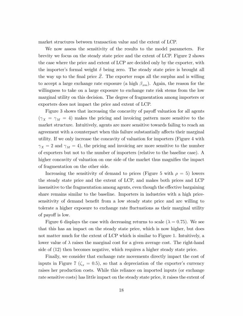
We now assess the sensitivity of the results to the model parameters. For

brevity we focus on the steady state price and the extent of LCP. Figure 2 shows

the case where the price and extent of LCP are decided only by the exporter, with

the importer’s formal weight δ being zero. The steady state price is brought all

the way up to the final price Z. The exporter reaps all the surplus and is willing

to accept a large exchange rate exposure (a high βxm). Again, the reason for the

willingness to take on a large exposure to exchange rate risk stems from the low

marginal utility on this decision. The degree of fragmentation among importers or

exporters does not impact the price and extent of LCP.

Figure 3 shows that increasing the concavity of payoff valuation for all agents

(γX = γM = 4) makes the pricing and invoicing pattern more sensitive to the

market structure. Intuitively, agents are more sensitive towards failing to reach an

agreement with a counterpart when this failure substantially affects their marginal

utility. If we only increase the concavity of valuation for importers (Figure 4 with

γX = 2 and γM = 4), the pricing and invoicing are more sensitive to the number

of exporters but not to the number of importers (relative to the baseline case). A

higher concavity of valuation on one side of the market thus magnifies the impact

of fragmentation on the other side.

Increasing the sensitivity of demand to prices (Figure 5 with ρ = 5) lowers

the steady state price and the extent of LCP, and makes both prices and LCP

insensitive to the fragmentation among agents, even though the effective bargaining

share remains similar to the baseline. Importers in industries with a high price-

sensitivity of demand benefit from a low steady state price and are willing to

tolerate a higher exposure to exchange rate fluctuations as their marginal utility

of payoff is low.

Figure 6 displays the case with decreasing returns to scale (λ = 0.75). We see

that this has an impact on the steady state price, which is now higher, but does

not matter much for the extent of LCP which is similar to Figure 1. Intuitively, a

lower value of λ raises the marginal cost for a given average cost. The right-hand

side of (12) then becomes negative, which requires a higher steady state price.

Finally, we consider that exchange rate movements directly impact the cost of

inputs in Figure 7 (ζx = 0.5), so that a depreciation of the exporter’s currency

raises her production costs. While this reliance on imported inputs (or exchange

rate sensitive costs) has little impact on the steady state price, it raises the extent of

18

LCP substantially, and makes the LCP share less sensitive to the market structure.

Intuitively, stabilizing the price in the importer’s currency provides more of a

hedging benefit to exporters, as a depreciation of their currency then increases

their unit revenue and thus offsets the increase in costs.

To sum up, our analysis shows that the extent of fragmentation among im-

porters and exporters impacts the effective bargaining weights, the prices, and the

extent of LCP. Interestingly, a higher bargaining power for importers benefits them

through a lower steady state price. This gives them high payoffs and thus lowers

their marginal utility. This in turns make them more tolerant towards volatility

and leads them to accept a high exposure to exchange rate fluctuations.

5.2 Intra-group heterogeneity

We now turn to the role of heterogeneity among exporter and importers. For

simplicity, we assume that there are two exporters, denoted by X1 and X2, and

two importers, denoted by M1 and M2. Without loss of generality we consider

that exporter 1 and importer 1 are relatively large. Specifically, the steady values

of the Qsetxm terms in (5) are:

QsetX1M1 = αψQset ; Qset

X1M2 = α (1− ψ) Qset

QsetX2M1 = (1− α)ψQset ; Qset

X2M2 = (1− α) (1− ψ) Qset

Qset is the total quantity exchange in the steady state. The coeffi cients α ∈ [0.5, 1]

and ψ ∈ [0.5, 1] denote the sizes of larger exporter and the larger importer, respec-

tively. The case of homogeneity (α = ψ = 0.5) corresponds to the fragmentation

case with X = M = 2.

As in the previous example, we begin by specifying the reference price Rmxm in

(5). We treat this reference price as an index of prices set by exporters to importer

m, written as:

Rmxm = Rm

m =[α [PX1m]1−ρ + (1− α) [PX2m]1−ρ

] 11−ρ (17)

where the first equality denotes that the reference price is the same for all exporters

selling to a given importer. For simplicity we assume that the final price Zm and

the input cost wx are the same for all importers and exporters.

The steady state solution takes the form of the pleasant exercise of solving

14 non-linear equations. The first two are the price indexes (17), one for each

19

importer. The next four equations are the shares (10)-(11), then we have four

effective bargaining weights (13), and finally four pricing equations (12). The

specific equations are given in the appendix.

Turning to the determination of the optimal degree of LCP,we set zm, qsetxm,

ζx and wx to be the same for all xm pairs for simplicity. A log linear approx-

imation of the reference price Rxm around the steady state implies that ηxm =

αβ1m + (1− α) β2m. Using this result, we obtain four variants of the optimum

LCP equation (14), one per importer-exporter pair. The relation for the 1, 2 pair

is presented in the appendix. The solution for the four invoicing shares is given by

inverting a linear system of four equations.

We illustrate our results with a numerical example, taking the same baseline

calibration as for the previous example. Figure 8 shows the effective bargaining

weights relative to the formal weight, δxm − δ, as a function of the heterogeneityamong exporters (α) and importers (β) for all exporter-importer pairs. The top

left panel considers the large importer’s weight vis-a-vis the large exporter (δX1M1),

and shows that importer bargaining weight increases with importer heterogeneity

(higher β) and decreases with the exporter heterogeneity (higher α).

The bottom left panel shows that the large importer’s bargaining weight vis-a-

vis the small exporter (δX2M1) is high and increases with importer heterogeneity,

especially at high levels of heterogeneity. While it also increases with exporter

heterogeneity, the effect is smaller. A mirror pattern is seen for the effective weight

of the small importer vis-a-vis the large exporter (δX1M2, top right panel), which is

relatively insensitive to the importer heterogeneity but falls rapidly as the exporter

heterogeneity increases. Finally, the small importer’s weight vis-a-vis the small

exporter (δX2M2, bottom right panel) is close to the formal weight and relatively

insensitive to heterogeneity.

The pattern for the effective bargaining weights is mirrored in the steady state

price (figure 9). The price is lower for sales to the larger importer (left panels)

than for sales to the small importer (right panels). The gap is more pronounced

when importer fragmentation is high, and for sales from the large exporter (top

panels).

The extent of LCP, βxm, is displayed in Figure 10 for the four importer-exporter

pairs. Starting from the point of full homogeneity (α = ψ = 0.5), the extent of

LCP between the large importer and the large exporter (top left panel) falls with

importer heterogeneity, but increases with exporter heterogeneity. This is a similar

20

pattern to the one of the steady state price in Figure 9. When the importer can

shift the surplus her way through a low steady state price, her marginal valuation

of profits is low. The importer then is little affected by exchange rate volatility

and more willing to be exposed to fluctuations resulting in low LCP. The similarity

between the steady state price and the extent of LCP is also seen for sales from the

large exporter to the small importer (top right panel). As the small importer carries

less weight than the large one, she receives a higher price, but also a more limited

exposure to exchange rate movements. The large importer also faces a smaller

degree of LCP on sales from the small exporter (bottom left panel) than on sales

from the large exporter (top left panel), reflecting the fact that she obtains a lower

price on purchases from the smaller exporter. The extent of LCP between the small

importer and small exporter (bottom right panel) increases with heterogeneity, but

that pair has a limited impact on the aggregate pattern with high heterogeneity.

To obtain summary measures of the pricing and invoicing, we compute the av-

erage and standard deviation of the steady state price and extent of LCP across the

four exporter-importer pairs, weighting each pair by its share in total steady state

transaction value. The results are presented in Figure 11. Exporter heterogeneity

raises the average price of traded goods (top left panel). While the cross-sectional

dispersion of prices (top right panel) is raised by heterogeneity of either exporters

or importers, the dispersion is increased more by exporter heterogeneity. The

extent of heterogeneity has a substantial impact on the average degree of LCP

(bottom left panel) which increases with exporter heterogeneity. Heterogeneity on

either side of the market raises the dispersion of LCP shares.

As the market structure impacts the steady state price, and hence the steady

state value of transactions, as well as the extent of LCP, we consider the link-

age between the two by computing the coeffi cient of correlation across the four

exporter-importer pairs between the steady state value of transactions and the ex-

tents of LCP (Figure 12). This correlation is negative when importer heterogeneity

dominates, but turns positive as exporter heterogeneity raises.

Our numerical example shows that the market structure has a sizable impact

on the effective bargaining weight, price, and extent of LCP across the various

importer-exporter pairs. This impact is also observed in aggregate terms, as the

average value and dispersion of prices and extents of LCP, as well as the corre-

lation between invoicing and transaction size, vary depending on the degrees of

heterogeneity among importers and exporters.

21

We now consider the impact of varying the model parameters along the same

lines as in the previous example. For brevity, we focus on the averages and standard

deviations of steady state prices and the extent of LCP, as well as the correlation

between transaction value and invoicing. In the case of unilateral decisions by the

exporters (δ = 0, not reported for brevity), the steady state price goes to the final

price and the exporter takes most of the exchange rate risk, as in the previous

example. The pricing and invoicing pattern is not affected by heterogeneity on

either side of the market.

Increasing the concavity of payoff valuation (γX = γM = 4) raises the average

extent of LCP somewhat (Figure 13 bottom left panel) and increases the dispersion

of prices and extent of LCP (right panels). The average value of prices and invoicing

remains sensitive to the amount of heterogeneity on both sides of the market. The

correlation between transaction value and invoicing remains close to the baseline

case (Figure 14). If payoffs are more concave only for importers (γX = 2 and

γM = 4), the average price and extent of LCP are further increased (Figure 15 left

panels).

Increasing the sensitivity of demand to prices (ρ = 5) substantially lower the

average price and the average extent of LCP, as importers’marginal utility is then

less sensitive to prices (Figure 17 left panels). The average price and invoicing is

also much less sensitive to the market structure. In addition, the cross sectional

dispersion of the two measures is reduced (right panels), and shifts the correlation

between transaction value and extent of LCP towards positive values (Figure 18).

Introducing decreasing returns to scale (λ = 0.75) raises the average price and

reduces the extent of LCP (Figure 19 left panels) and leads to more dispersion

in prices (top right panel). The dispersion in invoicing is now mostly driven by

importer heterogeneity. The market structure has a sizable impact on the average

price, and a more moderate one on the average extent of LCP. The correlation

between transaction value and extent of LCP shifts towards negative values (Fig-

ure 20). We finally consider a direct impact of the exchange rate on input costs

ζx = 0.5). This has little impact on prices (Figure 21 top panel) and raises the

average extent of LCP (bottom left panel) while lowering its dispersion somewhat.

The sensitivity of the average price and invoicing to the market structure remains

similar to the baseline case. The correlation between transaction value and invoic-

ing remains close to the baseline case (Figure 22).

22

5.3 Implications from the model

While our two specific examples focus on different dimensions of the model,

our analysis provides broad lessons that are relevant for understanding pricing and

invoicing patterns in international trade. These lessons arise when bargaining can

occur between exporters and importers.

First, the analysis should encompass all the dimensions of the contract that

are affected by bargaining. One may expect at first that a higher bargaining

power of risk-averse importers would lead them to reduce their exchange rate

exposure through higher LCP. Our analysis shows that the opposite is the case,

as the higher bargaining weight is reflected in a steady state price more favorable

to importers, which in turn reduces the marginal impact of exchange rate risk

on importers payoffs and leads them to accept more exchange rate exposure. A

different pattern would emerge if the bargaining took place only over the extent of

LCP, with the preset price set unilaterally by the exporter, in which case a higher

bargaining power of importers would raise the extent of LCP. These findings point

to the need for more research targeted at understanding the specific structures of

negotiations that occur between exporters and importers.

Second, the specific market structure matters not only at the level of individual

transactions but also in aggregate terms, as shown by our second example. This

insight points to the need for empirical studies of exchange rate exposure to un-

derstand the market structure at the micro level, even when the focus is on the

aggregate extent of LCP.

Third, our examples show that the extent of LCP is higher in situations where

exporters are more dominant, either because they are less fragmented (a low X

relative toM in the first example), or because their side of the market is dominated

by a few agents (a high α relative to ψ in the second example).

Fourth, the sensitivity of pricing and invoicing to market characteristics is mag-

nified when agents are more sensitive to risk, dampened in industries where de-

mand is more price-sensitive, and increased when exchange rate movements affect

exporters’costs.

Finally, the correlation between the value of specific transactions and their

reliance on LCP depends on the market structure. The correlation is positive

when large transactions reflect large exporters, but negative when they reflect

large importers.

23

6 Conclusion

This paper analyzes the determination of prices and exposure to exchange rate

fluctuations among exporters and importers through a simple model of bargaining.

This setting expands the theoretical analysis beyond the standard assumption of

unilateral choice by the exporter. We show that the market structure, reflecting

in the share of specific exporters and importers in each other’s total profits, has a

substantial impact on effective bargaining weights, prices, and exchange rate expo-

sure. This impact is not limited to specific exporter-importer pairs but also affects

the aggregate values of prices and exposure. A striking result of our analysis is that

powerful agents end up being more exposed to exchange rate fluctuations. This

reflects the fact that their power allows them to shift the steady state price in their

favor, which lowers their marginal utility and makes exchange rate fluctuations less

of a concern.

Our analysis is the first step towards building a bargaining view in the theory

of international trade pricing under uncertainty. Under this view understanding

aggregate prices requires one to take account of the microeconomic structure of

the market, such as the degrees of fragmentation and heterogeneity among ex-

porters and importers. A promising area of future research is to go beyond our

Nash bargaining solution and get more detailed evidence on the specific process of

interaction between importers and exporters in specific industries.

Another avenue for further work is to allow for prices to respond ex-post to

cost movements. It is reasonable to expect that this response will be substantially

affected by the market structure. Recall that the importer’s currency is used for

the invoicing when the importer’s weight is low, as she is then faced with a high

preset price, hence low profits and a high marginal valuation of profits. In line

with the finding of Gopinath, Itskhoki, and Rigobon (2010) that price adjustment

is low for U.S. imports invoiced in dollars, a reasonable conjecture is that in such a

situation the high marginal utility would also leads to limited movements of prices

when they can be adjusted.

24

7 Appendix

This technical appendix presents specific analytical points on the key aspects

of the model and its solution. A complete presentation of the technical aspects of

the paper is in an exhaustive technical appendix available on request.

7.1 Derivatives of the joint surplus

The derivatives with respect to the log of the fixed component of the price that

enter (8) are:

∂Θmxm

∂pfixxm= −E

∑X

i=1

exp

[zm + qsetim

−ρ(pfim − r

m,fim + (βim − ηim) s

) ]

− exp

[pfim − (1− βim) s+ qsetim

−ρ(pfim − r

m,fim + (βim − ηim) s

) ]

−γM

×

ρ exp

[zm + qsetxm

−ρ(pfxm − rm,fxm + (βxm − ηxm) s

) ]

+ (1− ρ) exp

[pfxm − (1− βxm) s+ qsetxm

−ρ(pfxm − rm,fxm + (βxm − ηxm) s

) ]

and:

∂Θxxm

∂pfixxm= E

∑M

j=1

exp

[pfxj + βxjs+ qsetxb

−ρ(pfxj − r

j,fxj +

(βxj − ηxj

)s) ]

− exp

[wx + ζxs+ 1

λqsetxj

− ρλ

(pfxj − r

j,fxj +

(βxj − ηxj

)s)− 1

λaxj

]

−γX

×

(1− ρ) exp

[pfxm + βxms+ qsetxm

−ρ(pfxm − rm,fxm + (βxm − ηxm) s

) ]

+ ρλ

exp

[wx + ζxs+ 1

λqsetxm

− ρλ

(pfxm − rm,fxm + (βxm − ηxm) s

)− 1

λaxm

]

25

The derivatives with respect to the exchange rate exposure in (9) are:

∂Θmxm

∂βxm= −E

∑X

i=1

exp

[zm + qsetim

−ρ(pfim − r

m,fim + (βim − ηim) s

) ]

− exp

[pfim − (1− βim) s+ qsetim

−ρ(pfim − r

m,fim + (βim − ηim) s

) ]

−γM

×

ρ exp

[zm + qsetxm

−ρ(pfxm − rm,fxm + (βxm − ηxm) s

) ]

+ (1− ρ) exp

[pfxm − (1− βxm) s+ qsetxm

−ρ(pfxm − rm,fxm + (βxm − ηxm) s

) ] s

and:

∂Θxxm

∂βxm= E

∑M

j=1

exp

[pfxj + βxjs+ qsetxb

−ρ(pfxj − r

j,fxj +

(βxj − ηxj

)s) ]

− exp

[wx + ζxs+ 1

λqsetxj

− ρλ

(pfxj − r

j,fxj +

(βxj − ηxj

)s)− 1

λaxj

]

−γX

×

(1− ρ) exp

[pfxm + βxms+ qsetxm

−ρ(pfxm − rm,fxm + (βxm − ηxm) s

) ]

+ ρλ

exp

[wx + ζxs+ 1

λqsetxm

− ρλ

(pfxm − rm,fxm + (βxm − ηxm) s

)− 1

λaxm

] s

7.2 Quadratic approximation

To write a quadratic approximation of (9), we first notice that left- and right-

hand sides are expressions of the form (the detailed expression for (9) is given in

a long technical appendix):

Φ =δ1

1− γ1

E

[(∑s1

(exp [a]− exp [b])

)−γ2(c1 exp [c] + h1 exp [h]) s

]

×

E(∑s2

(exp [d]− exp [e])

)1−γ1

− E( ∑

s2 (exp [d]− exp [e])

− (exp [f ]− exp [g])

)1−γ1

26

Bearing in mind that we expand around s = 0 and that Es = 0, we write:

Φ =δ1

1− γ1

(∑s2

(D − E

))1−γ1 (c1C + h1H

)(∑s1

(A− B

))−γ2

×

1−(

1− F − G∑s2

(D − E

))1−γ1E

−γ2

(∑s1

(A− B

))−1(∑

s1

(Aa− Bb

))s

+(c1C + h1H

)−1(c1Cc+ h1Hh

)s

We now apply this to the left-hand side of (9). The various elements are:

s1 = i = 1...X ; s2 = j = 1...M

δ1 = δ ; γ1 = γX ; γ2 = γM

c1 = ρ ; h1 = 1− ρa = zm + qsetim − ρ

(pfim − r

m,fim + (βim − ηim) s

)b = pfim − (1− βim) s+ qsetim − ρ

(pfim − r

m,fim + (βim − ηim) s

)c = zm + qsetxm − ρ

(pfxm − rm,fxm + (βxm − ηxm) s

)d = pfxj + βxjs+ qsetxj − ρ

(pfxj − r

j,fxj +

(βxj − ηxj

)s)

e = wx + ζxs+1

λqsetxj −

ρ

λ

(pfxj − r

j,fxj +

(βxj − ηxj

)s)− 1

λaxj

f = pfxm + βxms+ qsetxm − ρ(pfxm − rm,fxm + (βxm − ηxm) s

)g = wx + ζxs+

1

λqsetxm −

ρ

λ

(pfxm − rm,fxm + (βxm − ηxm) s

)− 1

λaxm

h = pfxm − (1− βxm) s+ qsetxm − ρ(pfxm − rm,fxm + (βxm − ηxm) s

)As all the pre-set component of all prices deviate from the steady-state allocation

only because of second moments, we can omit the various pf and rj,f from the

quadratic elements. We also recall that axm = 0 as Axm is constant. The quadratic

approximation of the left-hand side is then:

δ

1− γX

(X∑i=1

(Zm − Pim

)Qsetim

(Rmim

)ρ (Pim)−ρ)−γM

×(

M∑j=1

(Pxj − Wx

(Axj)− 1

λ(Qsetxj

) 1−λλ(Rjxj

)ρ 1−λλ(Pxj)−ρ 1−λ

λ

)Qsetxj

(Rjxj

)ρ (Pxj)−ρ)1−γX

×(ρZm + (1− ρ) Pxm

)Qsetxm

(Rmxm

)ρ (Pxm

)−ρ [1− (1− Πm

xm)1−γX]

×E

−γM (∑Xi=1 Πi

im

(Zm

Zm−PimEzmsEs2

+ PimZm−Pim (1− βim) +

Eqsetim s

Es2− ρ (βim − ηim)

))Es2

+(

ρZmρZm+(1−ρ)Pxm

EzmsEs2− (1−ρ)Pxm

ρZm+(1−ρ)Pxm(1− βxm) + Eqsetxms

Es2− ρ (βxm − ηxm)

)Es2

27

We now turn to the right-hand side of (9). The various elements are:

s1 = j = 1...M ; s2 = i = 1...X

δ1 = 1− δ ; γ1 = γM ; γ2 = γX

c1 = 1− ρ ; h1 =ρ

λ

a = pfxj + βxjs+ qsetxj − ρ(pfxj − r

j,fxj +

(βxj − ηxj

)s)

b = wx + ζxs+1

λqsetxj −

ρ

λ

(pfxj − r

j,fxj +

(βxj − ηxj

)s)− 1

λaxj

c = pfxm + βxms+ qsetxm − ρ(pfxm − rm,fxm + (βxm − ηxm) s

)d = zm + qsetim − ρ

(pfim − r

m,fim +

(βdim − ηdim

)sd)

e = pfim − (1− βim) s+ qsetim − ρ(pfim − r

m,fim + (βim − ηim) s

)f = zm + qsetxm − ρ

(pfxm − rm,fxm + (βxm − ηxm) s

)g = pfxm − (1− βxm) s+ qsetxm − ρ

(pfxm − rm,fxm + (βxm − ηxm) s

)h = wx + ζxs+

1

λqsetxm −

ρ

λ

(pfxm − rm,fxm + (βxm − ηxm) s

)− 1

λaxm

The quadratic approximation of the right-hand side is then:

1− δ1− γM

(X∑i=1

(Zm − Pim

)Qsetim

(Rmim

)ρ (Pim)−ρ)1−γM

×(

M∑j=1

(Pxj − Wx

(Axj)− 1

λ(Qsetxj

) 1−λλ(Rjxj

)ρ 1−λλ(Pxj)−ρ 1−λ

λ

)Qsetxj

(Rjxj

)ρ (Pxj)−ρ)−γX

×((1− ρ) Pxm + ρMCxm

)Qsetxm

(Rmxm

)ρ (Pxm

)−ρ [1− (1− Πx

xm)1−γM]

×E

−γx

∑Mj=1 Πj

xj

PxjPxj−Cxj

[βxj +

Eqsetxj s

Es2− ρ

(βxj − ηxj

)]− CxbPxj−Cxj

[EwxsEs2

+ ζx + 1λ

Eqsetxj s

Es2− ρ

λ

(βxj − ηxj

)]Es2

+

(1−ρ)Pxm(1−ρ)Pxm+ρMCxm

[βxm + Eqsetxms

Es2− ρ (βxm − ηxm)

]+ ρMCxm

(1−ρ)Pxm+ρMCxm

[EwxsEs2

+ ζx + 1λEqsetxmsEs2

− ρλ

(βxm − ηxm)] Es2

28

Combining our results, the approximation of (9) is written as:

0 = γM

(X∑i=1

Πiim

(Zm

Zm − PimEzms

Es2+

PimZm − Pim

(1− βim) +Eqsetim s

Es2− ρ (βim − ηim)

))

−γX

M∑j=1

Πjxj

PxjPxj−Cxj

[βxj +

Eqsetxj s

Es2− ρ

(βxj − ηxj

)]− CxjPxj−Cxj

[EwxsEs2

+ ζx + 1λ

Eqsetxj s

Es2− ρ

λ

(βxj − ηxj

)]

− ρZmρZm + (1− ρ) Pxm

Ezms

Es2+

(1− ρ) PxmρZm + (1− ρ) Pxm

(1− βxm)− Eqsetxms

Es2+ ρ (βxm − ηxm)

+(1− ρ) Pxm

(1− ρ) Pxm + ρMCxm

[βxm +

Eqsetxms

Es2− ρ (βxm − ηxm)

]+

ρMCxm

(1− ρ) Pxm + ρMCxm

[Ewxs

Es2+ ζx +

1

λ

Eqsetxms

Es2− ρ

λ(βxm − ηxm)

]which is (14) in the text after re-arranging terms.

7.3 Intra-group heterogeneity

The first two equations are the price indexes (17):

RM1 =[α[PX1M1

]1−ρ+ (1− α)

[PX2M1

]1−ρ] 11−ρ

RM2 =[α[PX1M2

]1−ρ+ (1− α)

[PX2M2

]1−ρ] 11−ρ

where we dropped the superscripts on the R for simplicity. The four shares between

importers and exporters (10)-(11) are (recall that ΠM2xm = 1 − ΠM1

xm , and ΠX2xm =

29

1− ΠX1xm:

ΠM1X1M1 =

1

1 +

(PX1M2−W(RM2)

ρ 1−λλ (PX1M2)

−ρ 1−λλ

)(1−ψ)(RM2)

ρ(PX1M2)

−ρ

(PX1M1−W(RM1)

ρ 1−λλ (PX1M1)

−ρ 1−λλ

)ψ(RM1)

ρ(PX1M1)

−ρ

ΠM1X2M1 =

1

1 +

(PX2M2−W(RM2)

ρ 1−λλ (PX2M2)

−ρ 1−λλ

)(1−ψ)(RM2)

ρ(PX2M2)

−ρ

(PX2M1−W(RM1)

ρ 1−λλ (PX2M1)

−ρ 1−λλ

)ψ(RM1)

ρ(PX2M1)

−ρ

ΠX1X1M1 =

1

1 +(Z−PX2M1)(1−α)(PX2M1)

−ρ

(Z−PX1M1)α(PX1M1)−ρ

ΠX1X1M2 =

1

1 +(Z−PX2M2)(1−α)(PX2M2)

−ρ

(Z−PX1M2)α(PX1M2)−ρ

The four effective bargaining weights (13) are:

δX1M1 =1

1 +(1−δ)H(ΠX1X1M1,γM)δH(ΠM1

X1M1,γX)

δX1M2 =1

1 +(1−δ)H(ΠX1X1M2,γM)δH((1−ΠM1

X1M1),γX)

δX2M1 =1

1 +(1−δ)H((1−ΠX1X1M1),γM)

δH(ΠM1X2M1,γX)

δX2M2 =1

1 +(1−δ)H((1−ΠX1X1M2),γM)δH((1−ΠM1

X2M1),γX)

Finally, we have four pricing equations (12). The specific equations are given in

the appendix. For the X1M1 pair we write:

δX1M1

(PX1M1 −

ρ

ρ− 1Z

)(PX1M1 − W

(RM1

)ρ 1−λλ(PX1M1

)−ρ 1−λλ

)=

(1− δX1M1

)(PX1M1 −

ρ

ρ− 1

1

λW(RM1

)ρ 1−λλ(PX1M1

)−ρ 1−λλ

)(Z − PX1M1

)

30

For the X1M2 pair we write:

δX1M2

(PX1M2 −

ρ

ρ− 1Z

)(PX1M2 − W

(RM2

)ρ 1−λλ(PX1M2

)−ρ 1−λλ

)=

(1− δX1M2

)(PX1M2 −

ρ

ρ− 1

1

λW(RM2

)ρ 1−λλ(PX1M2

)−ρ 1−λλ

)(Z − PX1M2

)For the X2M1 pair we write:

δX2M1

(PX2M1 −

ρ

ρ− 1Z

)(PX2M1 − W

(RM1

)ρ 1−λλ(PX2M1

)−ρ 1−λλ

)=

(1− δX2M1

)(PX2M1 −

ρ

ρ− 1

1

λW(RM1

)ρ 1−λλ(PX2M1

)−ρ 1−λλ

)(Z − PX2M1

)For the X2M2 pair we write:

δX2M2

(PX2M2 −

ρ

ρ− 1Z

)(PX2M2 − W

(RM2

)ρ 1−λλ(PX2M2

)−ρ 1−λλ

)=

(1− δX2M2

)(PX2M2 −

ρ

ρ− 1

1

λW(RM2

)ρ 1−λλ(PX2M2

)−ρ 1−λλ

)(Z − PX2M2

)There are four variants of (14) for the four importer-exporter pairs. For in-

stance, the one for the extent of LCP between importer M1 and exporter X2

31

is:

0 = −γXΠM1X1M1

(PX1M1

PX1M1−CX1M1− 1

λCX1M1

PX1M1−CX1M1

)ρα

+ PX1M1

PX1M1−CX1M1(1− ρ) + ρ

λCX1M1

PX1M1−CX1M1

βX1M1

−

(1−ρ)PX1M2

ρZ+(1−ρ)PX1M2− (1−ρ)PX1M2

(1−ρ)PX1B2+ρMCX1M2− ρMCX1M2

(1−ρ)PX1M2+ρMCX1M2

λ−1λρ

+γMΠX1X1M2

(PX1M2

Z−PX1M2+ ρ)−(γM − ρMCX1M2

(1−ρ)PX1M2+ρMCX1M2

λ−1λ

)ρα

+γXΠM2X1M2

(PX1M2

PX1M2−CX1M2− 1

λCX1M2

PX1M2−CX1M2

)ρα

+ PX1M2

PX1M2−CX1M2(1− ρ) + ρ

λCX1M2

PX1M2−CX1M2

βX1M2

−γXΠM1X1M1

(PX1M1

PX1B1 − CX1M1

− 1

λ

CX1M1

PX1M1 − CX1M1

)ρ (1− α) βX2M1

−

γMΠX2X2M2

(PX2M2

Z−PX2M2+ ρ)−(γM − ρMCX1M2

(1−ρ)PX1M2+ρMCX1M2

λ−1λ

)ρ (1− α)

+γXΠM2X1M2

(PX1M2

PX1M2−CX1M2− 1

λCX1M2

PX1M2−CX1M2

)ρ (1− α)

βX2M2

+

[(1− ρ) PX1M2

ρZ + (1− ρ) PX1M2

+ γM

(ΠX1X1M2

PX1M2

Z − PX1M2

+ ΠX2X1M2

PX2M2

Z − PM2M2

)]+

[γM

(ΠX1X1M2

Z

Z − PX1M2

+ ΠX2X2M2

Z

Z − PX2M2

)− ρZ

ρZ + (1− ρ) PX1M2

]Ezs

Es2

+

γM − ρMCX1M2

(1−ρ)PX1M2+ρMCX1M2

λ−1λ

−γXΠM1X1M1

(PX1M1

PX1M1−CX1M1− 1

λCX1M1

PX1M1−CX1M1

)−γXΠM2

X1M2

(PX1M2

PX1M2−CX1M2− 1

λCX1M2

PX1M2−CX1M2

) EqsetsEs2

+

[ρMCX1M2

(1−ρ)PX1M2+ρMCX1M2+ γXΠM1

X1M1CX1M1

PX1B1−CX1M1

+γXΠM2X1M2

CX1M2

PX1B2−CX1M2

](Ews

Es2+ ζ

)The other three relations are given in a separate detailed technical appendix.

32

References

[1] Auer, Raphael, and Raphael Schoenle, 2012. "Market structure and exchange

rate pass through," Swiss National Bank working paper 2012-14.

[2] Bacchetta, Philippe, and Eric van Wincoop, 2005. "A theory of the currency

denomination of international trade." Journal of International Economics, 67

(2), pp. 295—319.

[3] Berman, Nicolas, Philippe Martin, and Thierry Mayer, 2012. "How do dif-

ferent exporters react to exchange rate changes?" Quarterly Journal of Eco-

nomics, 127 (1), pp. 437-492.

[4] Camera, Gabriele, and Cemil Selcuk, 2009. "Price dispersion with directed

search", Journal of the European Economic Association 7(6), pp. 1193-1224.

[5] Chipty, Tasneem, and Christopher Snyder, 1999. "The role of firm size in

a bilateral bargaining: a study of the cable television industry", Review of

Economics and Statistics 81(2), pp. 326-340.

[6] DeGraba, Patrick, 2005. "Quantity discounts from risk averse sellers", FTC

working paper 276.

[7] DeBlas, Beatriz and Katheryn Niles Russ, 2010. "Understanding markups in

the open economy under Bertrand competition", NBER working paper 16587.

[8] Devereux, Michael, Charles Engel, and Peter Storgaard, 2004. "Endogenous

exchange rate pass-through when nominal prices are set in advance." Journal

of International Economics, 63 (2), pp. 263—291.

[9] Devereux, Michael, and Shouyong Shi, 2013. "Vehicle currency", International

Economic Review, forthcoming.

[10] Dowbson, Paul, and Michael Waterson, 1997. "Countervailing power and con-

sumer prices", The Economic Journal 107 (441), pp. 418-430.

[11] Engel, Charles, 2006. "Equivalence results for optimal pass-through, optimal

indexing to exchange rates, and optimal choice of currency for export pricing,"

Journal of the European Economic Association, vol. 4 (6), pp. 1249-1260.

33

[12] Friberg, Richard. 1998. "In which Currency Should Exporters Set their

Prices?" Journal of International Economics, 45(1), pp. 59-76.

[13] Friberg, Richard, and Fredrik Wilander, 2008. "The currency denomination of

exports —Aquestionnaire study", Journal of International Economics, 75(1),

pp. 54-69.

[14] Garetto, Stefania, 2012. "Firms’heterogeneity and incomplete pass through,"

manuscript Boston University.

[15] Goldberg, Linda, and Cédric Tille, 2011. "Micro, Macro, and Strategic Forces

in International Trade Invoicing", Federal Reserve Bank of New York staff

report 405.

[16] Goldberg, Linda, and Cédric Tille, 2008. "Vehicle currency use in international

trade", Journal of International Economics, 76, pp. 177-192.

[17] Gopinath, Gita, Oleg Itskhoki, and Roberto Rigobon 2010. "Currency Choice

and Exchange Rate Pass-Through", American Economic Review, 100 (1), pp.

304—336.

[18] Hellerstein, Rebecca, 2008. "Who bears the cost of a change in the exchange

rate? Pass-through accounting for the case of beer," Journal of international

economics, 76 (1), pp.14-32

[19] Horn, Henrick, and Asher Wolinsky, 1988. "Bilateral monopolies and incen-

tives for mergers", Rand Journal of Economics 19 (3), pp. 408-419.

[20] Inderst, Roman, and Christian Wey, 2003. "Bargaining, mergers and technol-

ogy choice in bilaterally oligopolistic industries", Rand Journal of Economics,

34 (1), pp. 1-19.

[21] Ito, Takatoshi, Satoshi Koibuchi, Kiyotaka Sato and Junko Shimizu, 2012.

“The choice of an invoicing currency by globally operating firms: A firm-level

analysis of Japanese exporters’invoicing behavior”, International Journal of

Finance and Economics, 17 (4), pp. 305-320.

[22] Normann, Hans-Theo, Bradley Ruffl e, and Christopher Snyder, 2007. "Do

buyer-size discounts depend on the curvature of the surplus function? Exper-

34

imental tests of bargaining models", Rand Journal of Economics 38 (3), pp.

747-767.

[23] Novy, Dennis, 2006. “Hedge your Costs: Exchange Rate Risk and Endogenous

Currency Invoicing”, Warwick economic research paper 765.

[24] Selcuk, Cemil, 2012. "Trading mechanism selection with directed search when

buyers are risk averse", Economics Letters, 115 (2), pp. 207—210.

[25] Tille, Cédric, and Eric van Wincoop, 2010. "International Capital Flows.",

Journal of International Economics, vol. 80, pp. 157-175.

35

Figure 1: Pricing and invoicing, fragmentation case

M denotes the number of (identical) importers. The higher M the more fragmented are importers across many small ones. X denotes the number of (identical) exporters. The higher X the more fragmented are exporters across many small ones. Parameters: = 0.5, X = 2, M = 2, = 2, = 1, Wx = 1, Qset = 10, x = 0, E(qset s)/(Es2) =0, E(wx s)/(Es2) =0, E(z s)/(Es2) =0.

Figure 2: Role of formal bargaining weight, fragmentation case

M denotes the number of (identical) importers. The higher M the more fragmented are importers across many small ones. X denotes the number of (identical) exporters. The higher X the more fragmented are exporters across many small ones. Parameters are as in the baseline of Figure 2, except for = 0 instead of = 0.5. Figure 3: Role of overall risk aversion, fragmentation case

M denotes the number of (identical) importers. The higher M the more fragmented are importers across many small ones. X denotes the number of (identical) exporters. The higher X the more fragmented are exporters across many small ones. Parameters are as in the baseline of Figure 2, except for X = 4, M = 4 instead of X = 2, M = 2.

Figure 4: Role of importer’s risk aversion, fragmentation case

M denotes the number of (identical) importers. The higher M the more fragmented are importers across many small ones. X denotes the number of (identical) exporters. The higher X the more fragmented are exporters across many small ones. Parameters are as in the baseline of Figure 2, except for M = 4 instead of M = 2. Figure 5: Role of price sensitivity, fragmentation case

M denotes the number of (identical) importers. The higher M the more fragmented are importers across many small ones. X denotes the number of (identical) exporters. The higher X the more fragmented are exporters across many small ones. Parameters are as in the baseline of Figure 2, except for = 5 instead of = 2.

Figure 6: Role of returns to scale, fragmentation case

M denotes the number of (identical) importers. The higher M the more fragmented are importers across many small ones. X denotes the number of (identical) exporters. The higher X the more fragmented are exporters across many small ones. Parameters are as in the baseline of Figure 2, except for = 0.75 instead of = 1. Figure 7: Role of link between cost and exchange rate, fragmentation case

M denotes the number of (identical) importers. The higher M the more fragmented are importers across many small ones. X denotes the number of (identical) exporters. The higher X the more fragmented are exporters across many small ones. Parameters are as in the baseline of Figure 2, except for x = 0.5 instead of x = 0.

Figure 8: Effective bargaining weight of importer (relative to formal weight) xm

~ , heterogeneity case

denotes the size of the larger exporter. The higher the more heterogeneous are exporters between a large exporter and a small one denotes the size of the larger importer. The higher the more heterogeneous are importers between a large importer and a small one Parameters: = 0.5, X = 2, M = 2, = 2, = 1, Wx = 1, Qset = 10, x = 0, E(qset s)/(Es2) =0, E(wx s)/(Es2) =0, E(z s)/(Es2) =0.

Figure 9: Steady state price xmP , heterogeneity case

denotes the size of the larger exporter. The higher the more heterogeneous are exporters between a large exporter and a small one denotes the size of the larger importer. The higher the more heterogeneous are importers between a large importer and a small one Parameters: = 0.5, X = 2, M = 2, = 2, = 1, Wx = 1, Qset = 10, x = 0, E(qset s)/(Es2) =0, E(wx s)/(Es2) =0, E(z s)/(Es2) =0.

Figure 10: LCP share xm , heterogeneity case

denotes the size of the larger exporter. The higher the more heterogeneous are exporters between a large exporter and a small one denotes the size of the larger importer. The higher the more heterogeneous are importers between a large importer and a small one Parameters: = 0.5, X = 2, M = 2, = 2, = 1, Wx = 1, Qset = 10, x = 0, E(qset s)/(Es2) =0, E(wx s)/(Es2) =0, E(z s)/(Es2) =0.

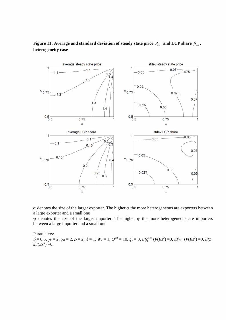
Figure 11: Average and standard deviation of steady state price xmP

and LCP share xm , heterogeneity case

denotes the size of the larger exporter. The higher the more heterogeneous are exporters between a large exporter and a small one denotes the size of the larger importer. The higher the more heterogeneous are importers between a large importer and a small one Parameters: = 0.5, X = 2, M = 2, = 2, = 1, Wx = 1, Qset = 10, x = 0, E(qset s)/(Es2) =0, E(wx s)/(Es2) =0, E(z s)/(Es2) =0.

Figure 12: Correlation between transaction value xmxmQP

and LCP share xm , heterogeneity case

denotes the size of the larger exporter. The higher the more heterogeneous are exporters between a large exporter and a small one denotes the size of the larger importer. The higher the more heterogeneous are importers between a large importer and a small one Parameters: = 0.5, X = 2, M = 2, = 2, = 1, Wx = 1, Qset = 10, x = 0, E(qset s)/(Es2) =0, E(wx s)/(Es2) =0, E(z s)/(Es2) =0.

Figure 13: Role of overall risk aversion, Average and standard deviation of steady price xmP

and LCP share xm , heterogeneity case

denotes the size of the larger exporter. The higher the more heterogeneous are exporters between a large exporter and a small one denotes the size of the larger importer. The higher the more heterogeneous are importers between a large importer and a small one Parameters are as in the baseline of Figures 8-12, except for X = 4, M = 4 instead of X = 2, M = 2.

Figure 14: Role of overall risk aversion, Correlation between transaction value xmxmQP

and LCP share xm , heterogeneity case

denotes the size of the larger exporter. The higher the more heterogeneous are exporters between a large exporter and a small one denotes the size of the larger importer. The higher the more heterogeneous are importers between a large importer and a small one Parameters are as in the baseline of Figures 8-12, except for X = 4, M = 4 instead of X = 2, M = 2.

Figure 15: Role of importer’s risk aversion, Average and standard deviation of steady state price xmP

and LCP share xm , heterogeneity case

denotes the size of the larger exporter. The higher the more heterogeneous are exporters between a large exporter and a small one denotes the size of the larger importer. The higher the more heterogeneous are importers between a large importer and a small one Parameters are as in the baseline of Figures 8-12, except for M = 4 instead of M = 2.

Figure 16: Role of importer’s risk aversion, Correlation between transaction value xmxmQP

and LCP share xm , heterogeneity case

denotes the size of the larger exporter. The higher the more heterogeneous are exporters between a large exporter and a small one denotes the size of the larger importer. The higher the more heterogeneous are importers between a large importer and a small one Parameters are as in the baseline of Figures 8-12, except for M = 4 instead of M = 2.

Figure 17: Role of price sensitivity, Average and standard deviation of steady state price xmP

and LCP share xm , heterogeneity case

denotes the size of the larger exporter. The higher the more heterogeneous are exporters between a large exporter and a small one denotes the size of the larger importer. The higher the more heterogeneous are importers between a large importer and a small one Parameters are as in the baseline of Figures 8-12, except for = 5 instead of = 2.

Figure 18: Role of price sensitivity, Correlation between transaction value xmxmQP

and LCP share xm , heterogeneity case

denotes the size of the larger exporter. The higher the more heterogeneous are exporters between a large exporter and a small one denotes the size of the larger importer. The higher the more heterogeneous are importers between a large importer and a small one Parameters are as in the baseline of Figures 8-12, except for = 5 instead of = 2.

Figure 19: Role of returns to scale, Average and standard deviation of steady state price xmP

and LCP share xm , heterogeneity case

denotes the size of the larger exporter. The higher the more heterogeneous are exporters between a large exporter and a small one denotes the size of the larger importer. The higher the more heterogeneous are importers between a large importer and a small one Parameters are as in the baseline of Figures 8-12, except for = 0.75 instead of = 1.

Figure 20: Role of returns to scale, Correlation between transaction value xmxmQP

and LCP share xm , heterogeneity case

denotes the size of the larger exporter. The higher the more heterogeneous are exporters between a large exporter and a small one denotes the size of the larger importer. The higher the more heterogeneous are importers between a large importer and a small one Parameters are as in the baseline of Figures 8-12, except for = 0.75 instead of = 1.

Figure 21: Role of link between cost and exchange rate, Average and standard deviation of steady state price xmP

and LCP share xm , heterogeneity case

denotes the size of the larger exporter. The higher the more heterogeneous are exporters between a large exporter and a small one denotes the size of the larger importer. The higher the more heterogeneous are importers between a large importer and a small one Parameters are as in the baseline of Figures 8-12, except for x = 0.5 instead of x = 0.

Figure 22: Role of link between cost and exchange rate, Correlation between transaction value xmxmQP

and LCP share xm , heterogeneity case

denotes the size of the larger exporter. The higher the more heterogeneous are exporters between a large exporter and a small one denotes the size of the larger importer. The higher the more heterogeneous are importers between a large importer and a small one Parameters are as in the baseline of Figures 8-12, except for x = 0.5 instead of x = 0.