A

Appendix:Radiometry and Photometry

This appendix deals with the photometric and radiometric variables thatare useful in setting and understanding problems about color and energyexchange.

All eletromagnetic radiation transfers energy, called radiant energy.Radiometry is the science of the measurement of the physical variables as-sociated with the propagation and exchange of radiant energy. Photometry isthe branch of radiometry that deals with these variables from the viewpointof visual responses; that is, it studies how radiant energy is perceived by anobserver. Thus, radiometry in general deals with physical processes, whilephotometry deals with psychophysical ones.

A.1 Radiometry

Although an understanding of the physics of electromagnetic waves is impor-tant in the study of light–matter interaction, we need not be concerned withthe nature of electromagnetism in the study of radiometry and photometry. Itis enough to know that radiant energy flows through space; the fundamentalvariable involved is the flux through a surface, that is, the rate at which radi-ant energy is transferred through a surface. This notion is therefore analogousto the notion of an electric current or to the flow of matter in fluid dynamics.

In contrast with the situation in fluid dynamics, however, there exist pointsources of radiant energy, and indeed they are of great importance in radio-metry. To define the radiometric variables associated with point sources, weintroduce the notion of solid angles.

Solid Angles

In the plane, angles can be regarded as a measure of apparent length froman observer’s viewpoint. To compute the angle subtended by an object when

440 A Appendix: Radiometry and Photometry

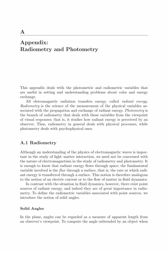
Fig. A.1. Angles and radial projection.

observed from a point O, we project the object radially onto the unit circlecentered at O and measure the arc determined by this projection; this is howbig the object looks to someone stationed at O (Figure A.1).

We can also use a circle of radius other than 1, but in this case we mustdivide the length of the projected arc by the radius of the circle. Thus, anglesare dimensionless quantities. Radians and other units of angle measurementare a notational device to avoid confusion when working with such measure-ments: a radian is simply the number 1; a degree is the number π/180; andso on.

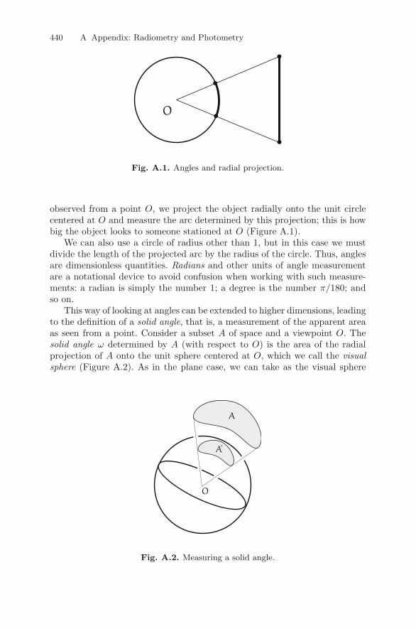
This way of looking at angles can be extended to higher dimensions, leadingto the definition of a solid angle, that is, a measurement of the apparent areaas seen from a point. Consider a subset A of space and a viewpoint O. Thesolid angle ω determined by A (with respect to O) is the area of the radialprojection of A onto the unit sphere centered at O, which we call the visualsphere (Figure A.2). As in the plane case, we can take as the visual sphere

Fig. A.2. Measuring a solid angle.

A.1 Radiometry 441

a sphere of arbitrary radius r �= 1, but then we must divide the area of theprojection by the square of the radius. Thus, the solid angle is given by

ω =Area(A′)

r2. (A.1)

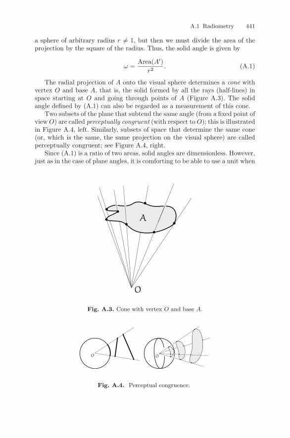
The radial projection of A onto the visual sphere determines a cone withvertex O and base A, that is, the solid formed by all the rays (half-lines) inspace starting at O and going through points of A (Figure A.3). The solidangle defined by (A.1) can also be regarded as a measurement of this cone.

Two subsets of the plane that subtend the same angle (from a fixed point ofview O) are called perceptually congruent (with respect to O); this is illustratedin Figure A.4, left. Similarly, subsets of space that determine the same cone(or, which is the same, the same projection on the visual sphere) are calledperceptually congruent; see Figure A.4, right.

Since (A.1) is a ratio of two areas, solid angles are dimensionless. However,just as in the case of plane angles, it is comforting to be able to use a unit when

Fig. A.3. Cone with vertex O and base A.

Fig. A.4. Perceptual congruence.

442 A Appendix: Radiometry and Photometry

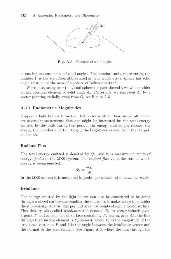
Fig. A.5. Element of solid angle.

discussing measurements of solid angles. The standard unit, representing thenumber 1, is the steradian, abbreviated sr. The whole visual sphere has solidangle 4π sr, since the area of a sphere of radius r is 4πr2.

When integrating over the visual sphere (or part thereof), we will consideran infinitesimal element of solid angle dω. Pictorially, we represent dω by avector pointing radially away from O; see Figure A.5.

A.1.1 Radiometric Magnitudes

Suppose a light bulb is turned on, left on for a while, then turned off. Thereare several measurements that one might be interested in: the total energyemitted by the bulb during this period; the energy emitted per second; theenergy that reaches a certain target; the brightness as seen from that target;and so on.

Radiant Flux

The total energy emitted is denoted by Qe, and it is measured in units ofenergy: joules in the MKS system. The radiant flux Φe is the rate at whichenergy is being emitted:

Φe =dQe

dt.

In the MKS system it is measured in joules per second, also known as watts.

Irradiance

The energy emitted by the light source can also be considered to be goingthrough a closed surface surrounding the source, so it makes sense to considerthe flux density—that is, flux per unit area—at points of such a closed surface.Flux density, also called irradiance and denoted Ee, is vector-valued: givena point P and an element of surface containing P , having area dA, the fluxthrough that surface element is Ee cos θdA, where Ee is the magnitude of theirradiance vector at P and θ is the angle between the irradiance vector andthe normal to the area element (see Figure A.6, where the flux through the

A.1 Radiometry 443

Fig. A.6. The amount of radiant energy crossing a surface per unit time dependson which way the surface faces.

surface is negative on the left, zero in the middle, and positive on the right).Loosely, we can write

Ee =dΦe

dA.

Irradiance is measured (in the MKS system) in watts per square meter.

Radiant Intensity

The irradiance depends, of course, on how far the point of measurement isfrom the source (and usually also on the direction as seen from the source). Itis often useful to work instead with a magnitude that is associated with thesource itself. For a point light source, this is easy: we just consider flux persolid angle instead of flux per area. The radiant intensity Ie of a point sourceis defined as

Ie =dΦe

dω,

where dω is the element of solid angle as seen from the source and is measuredin watts per steradian. (Note that this does not make sense unless the lightsource has negligible extension, since the notion of solid angle depends essen-tially on the choice of an origin.) The radiant intensity is a function of thedirection as seen from the source. When we integrate it over all directions, werecover the total flux, Φe =

∫Iedω. For a source that sheds light uniformly in

all directions, Ie is constant and Φe = 4πIe.Clearly, the flux density an observer perceives at a distance d from the

source is Ee = Ie/d2.

Radiance

This concept can be adapted to the case of nonpoint light sources, as follows.Consider a surface S that delimits the source in question—the surface of alight bulb, say, or a sphere around it. (The light need not be generated on S;it is the flux through S that concerns us.) If we take an element of the surface,of area dA, we can regard it as a point source and look at its radiant intensity

444 A Appendix: Radiometry and Photometry

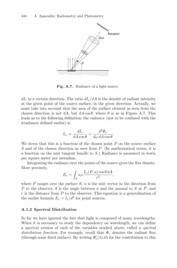
Fig. A.7. Radiance of a light source.

dIe in a certain direction. The ratio dIe/dA is the density of radiant intensityat the given point of the source surface, in the given direction. Actually, wemust take into account that the area of the surface element as seen from thechosen direction is not dA, but dA cos θ, where θ is as in Figure A.7. Thisleads us to the following definition: the radiance (not to be confused with theirradiance defined earlier) is

Le =dIe

dA cos θ=

d2Φe

dω dA cos θ.

We stress that this is a function of the chosen point P on the source surfaceS and of the chosen direction as seen from P . (In mathematical terms, it isa function on the unit tangent bundle to S.) Radiance is measured in wattsper square meter per steradian.

Integrating the radiance over the points of the source gives the flux density.More precisely,

Ee =∫

S

uPLe(P, u) cos θ dA

r2,

where P ranges over the surface S, u is the unit vector in the direction fromP to the observer, θ is the angle between u and the normal to S at P , andr is the distance from P to the observer. This equation is a generalization ofthe earlier formula Ee = Ie/d2 for point sources.

A.1.2 Spectral Distribution

So far we have ignored the fact that light is composed of many wavelengths.When it is necessary to study the dependency on wavelength, we can definea spectral version of each of the variables studied above, called a spectraldistribution function. For example, recall that Φe denotes the radiant flux(through some fixed surface). By writing Φ′

e(λ) dλ for the contribution to this

A.1 Radiometry 445

Fig. A.8. Spectral distribution of a radiometric variable.

flux that has wavelength between λ and λ + dλ, where dλ is an infinitesimalwavelength, we obtain the spectral distribution of flux Φ′

e(λ). Clearly, we have

Φe =∫ +∞

−∞Φ′

e(λ) dλ.

Figure A.8 shows a possible spectral distribution.The radiometric variables we have introduced are also functions of time,

and some are also functions of position and/or direction, as we have seen.These dependences are essential in image synthesis and animation. In col-orimetry, however, we usually concentrate on wavelength dependence.

Black-Body Radiation

Every material emits radiant energy, at a rate that increases rapidly withthe temperature. The spectral distribution of this radiation depends on thetemperature and on the nature of the emitter, but at each frequency andtemperature the radiant flux of a physical body is bounded by a certain limitpredicted by quantum mechanics. A black body is an ideal object that emitsexactly the predicted maximum amount of energy at each temperature. Theradiance of a black body is given by Planck’s equation,

Le(λ) =2c2h

λ5(ehc/(kTλ) − 1),

where T is the temperature (in degrees Kelvin), h = 6.6260755× 10−34 joule-second is Planck’s constant, c = 2.99792458 × 108 meters per second is thespeed of light, and k = 1.380658 × 10−23 joule per degree is Boltzmann’sconstant. Figure A.9 shows the graph of this function for several temperaturevalues.

It is possible to construct, for experimental purposes, devices that approx-imate very well the emission of a black body, at least within a certain rangeof frequencies and temperatures.

446 A Appendix: Radiometry and Photometry

Fig. A.9. Spectral distribution of black-body radiance.

Standard Illuminants

Paint manufacturers give fancy names to dozens of shades that mere mortalswould call white. Because the designation “white” is applied so loosely andsubjectively, it is essential (for example, in calibration procedures or in thespecification of color systems) to specify exactly the spectral distribution ofcertain colors, taken as standard whites, or standard illuminants. The CIE, orInternational Commission on Illumination, defines illuminant A as the spectraldistribution of a black body at 2856◦K; this spectrum can be approximatedby the light of an incandescent tungsten filament. Illuminant B, which cor-responds approximately to direct solar light, has by definition the spectraldistribution of a black body at 4874◦K, whereas illuminant C has the spec-tral distribution of a black body at 6774◦K. A number of illuminants attemptto approximate daylight under different conditions: D55, D65, and D75 corre-spond to temperatures of 5500◦K, 6500◦K, and 7500◦K, respectively. Finally,Illuminant E is defined by an ideal source whose spectral distribution is flatin terms of energy; for this reason it is also called the equal-energy white. Thecolor of such a source is perceptually the same as that of a black body ataround 6000◦K, but its spectral distribution is of course different.

More details on these illuminants and other standards can be found in theliterature cited in Section A.3.

A.2 Photometric Variables

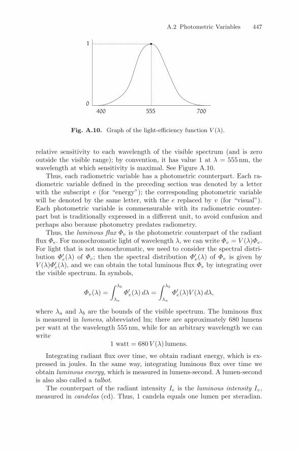
In photometry our interest shifts from purely physical characteristics of lightto the question of how a human observer perceives light. To a first approxima-tion, this means that radiometric variables, such as the energy flux reachingthe observer, should be weighted according to the human eye’s sensitivityto light of that wavelength, which is encoded in the light-efficiency functionV (λ), discussed in Section 4.6. Recall that this function measures the eye’s

A.2 Photometric Variables 447

Fig. A.10. Graph of the light-efficiency function V (λ).

relative sensitivity to each wavelength of the visible spectrum (and is zerooutside the visible range); by convention, it has value 1 at λ = 555 nm, thewavelength at which sensitivity is maximal. See Figure A.10.

Thus, each radiometric variable has a photometric counterpart. Each ra-diometric variable defined in the preceding section was denoted by a letterwith the subscript e (for “energy”); the corresponding photometric variablewill be denoted by the same letter, with the e replaced by v (for “visual”).Each photometric variable is commensurable with its radiometric counter-part but is traditionally expressed in a different unit, to avoid confusion andperhaps also because photometry predates radiometry.

Thus, the luminous flux Φv is the photometric counterpart of the radiantflux Φe. For monochromatic light of wavelength λ, we can write Φv = V (λ)Φe.For light that is not monochromatic, we need to consider the spectral distri-bution Φ′

e(λ) of Φe; then the spectral distribution Φ′v(λ) of Φv is given by

V (λ)Φ′e(λ), and we can obtain the total luminous flux Φe by integrating over

the visible spectrum. In symbols,

Φv(λ) =∫ λb

λa

Φ′v(λ) dλ =

∫ λb

λa

Φ′e(λ)V (λ) dλ,

where λa and λb are the bounds of the visible spectrum. The luminous fluxis measured in lumens, abbreviated lm; there are approximately 680 lumensper watt at the wavelength 555 nm, while for an arbitrary wavelength we canwrite

1 watt = 680V (λ) lumens.

Integrating radiant flux over time, we obtain radiant energy, which is ex-pressed in joules. In the same way, integrating luminous flux over time weobtain luminous energy, which is measured in lumens-second. A lumen-secondis also also called a talbot.

The counterpart of the radiant intensity Ie is the luminous intensity Iv,measured in candelas (cd). Thus, 1 candela equals one lumen per steradian.

448 A Appendix: Radiometry and Photometry

It is in fact the candela that is taken as the fundamental unit of photometricmagnitudes: by definition, one candela is the luminous intensity in the per-pendicular direction of a surface of 1/600,000 of a square meter of a blackbodyat the temperature of fusion of platinum (approximately 1773◦C, 2046◦K, or3223◦F).

The photometric counterpart of irradiance is illuminance, measured inlumens per square meters. A lumen per square meter is also called a lux (lx).

The photometric counterpart of radiance is luminance, Lv. Luminance is aphotometric variable that corresponds most closely to the notion of brightnessperceived by the eye. It is measured in candelas per square meter.

Other photometric and radiometric variables are used in the literature,including some that are specifically geared toward computer graphics needs.Moreover, for the variables discussed here, there are other units in use, themost important of which is the foot-candle, a unit of illuminance equal to onelumen per square foot, or 10.7639 lux.

Table 12.1 summarizes the preceding discussion.

Table 12.1. Photometric and radiometric variables.

Radiometric variable Symbol Unit

radiant energy Qe J (joule)radiant flux Φe W (watt)irradiance Ee W/m2

radiant intensity Ie W/srradiance Le W/sr·m2

Photometric variable Symbol Unitluminous energy Qv lm·s (talbot)luminous flux Φv lm (lumen)illuminance Ev lm/m2 (lux = lx)luminous intensity Iv lm/sr (candela = cd)luminance Lv cd/m2 = lx/sr

Example: Spectral Luminance

Consider a light source whose radiance spectral distribution function is known;let it be C(λ), in units of W/sr·m2. The corresponding luminance distributionfunction is therefore

680C(λ)V (λ),

in units of cd/m2. The total luminance of the source can then be computedby integrating over the visible spectrum:

Lv = 680∫ λb

λa

C(λ)V (λ) dλ,

in units of cd/m2.

A.3 Comments and References 449

In performing integrals such as this one in practice, we must be aware theV (λ) is known from tabulated values at a discrete set of points λa = λ0 < λ1 <· · · < λn = λb. The integral therefore must be approximated numerically; thesimplest method is to use the trapezoid rule, so that

Lv = 680n∑

i=1

12

(C(λi)V (λi) + C(λi−1)V (λi−1)

)(λi − λi−1).

Better results can be obtained by using, for example, Gaussian quadrature.

A.3 Comments and References

The purpose of this appendix is simply to give self-contained definitions of themain variables of interest in radiometry and photometry, such as the lumi-nance of a color, without interfering with the exposition in Chapter 4. It doesnot attempt to be a complete exposition of the subject. In particular, we haveomitted any mention of the illumination equation, which is of fundamentalimportance in image synthesis. A concise but good exposition of radiometryand photometry geared toward computer graphics can be found in (Kajiya1990).

A comprehensive treatment of radiometry and photometry, describingphysical experiments and including quantitative information on standard il-luminants, can be found in (Wyszecki and Stiles 1982).

There are whole books devoted to colorimetry and photometry in general;a good one is (Walsh 1958). The subject is also covered in many optics books,such as (Klein and Furtak 1986).

References

[Kajiya 1990]Kajiya, J. (1990). Radiometry and photometry for computergraphics. SIGGRAPH ’90 Course Notes.

[Klein and Furtak 1986]Klein, M. and Furtak, T. (1986). Optics, 2nd ed.John Wiley and Sons, New York.

[Walsh 1958]Walsh, J. T. (1958). Photometry. Dover, New York.[Wyszecki and Stiles 1982]Wyszecki, G. and Stiles, W. S. (1982). Color

Science. John Wiley & Sons, New York.

Index

support medium, 417dot dispersion, 327three-dimensional image, 137two-dimensional image, 137

abstraction paradigms, 3, 9achromatic color point, 98achromatic line, 98ACM, 133acuity visual

angle de, 314adaptive filter, 32addition of signals, 32Adobe Systems, 436algorithm

Floyd–Steinberg, 330median cut, 305populosity, 303

algorithmscluster ordered dithering, 429digital halftone, 314

aliasing, 191and reconstruction, 211error, 192

alpha channel, 369, 370alpha-channel compositing, 374amplitude discretization, 413analog signal, 18analog-electronic image, 413analytic sampling, 195angle of visual acuity, 314animation, 410animation morphing, 411

Antunes, Andre, VIII

area sampling, 31, 145, 195atlas

of color, 127

AuthorAdelson, E., 185Anderson, C., 185

Barnsley, Michael, 357Barsky, Brian, 384Bayer, B., 342

Beatty, J. C., 436Bergen, J., 185Bloomenthal, James, 384

Burt, P., 185Buzo, A., 311Carpenter, Loren, 384

Catmull, Edwin, 184, 436Clark, R., 357Cole, A., 343

Cook, Rob, 184Costa, Bruno, 215, 384, 412Cowan, W. B., 436

Crow, Frank, 215Darsa, Lucia, 215, 384, 412Daubechies, Ingrid, 185

Davidson, J., 184DeMarsh, LeRoy, 435Dubois, Eric, 216

Duff, Tom, 384Fishkin, K. P., 384Fiume, Eugene, 215, 311, 384

Floyd, R., 342Foley, James, 133

451

452 Index

Fournier, Alan, 384Furtak, Thoms, 449Geist, R., 343Giorgianni, Edward, 435Glassner, Andrew, 215Gomes, Jonas, 215, 343, 412Gonzalez, R., 145Gotsman, C., 343Gray, R., 311Greenberg, Donald, 133Grey, F., 215Hall, Roy, 134, 184, 435Hamill, P., 341Harada, K., 384Harmon, L., 341Haykin S., 358Heckbert, Paul, 215, 310, 311Hilbert, David, 334Hurd, Lyman, 357Ishizaki, T., 384Jain, A., 145, 215, 357Jarvis, J. F., 341Joblove, G., 133Judice, C. N., 341Kajiya, James, 449Kak, A. C., 435Kay, David C., 435Klein, Miles, 449Knowlton, K., 341Knuth, Donald, 342Kurland, M., 342Lamming, M., 436Levine, John R., 435Lim, J. S., 357Limb, J. O., 341Linde, Y., 311Lippel, B., 342Lloyd, S., 311Max, J., 311Mendelsohn, M., 343Mertz, P., 215Meyer, Gary, 134Mitchell, ???, 215Murray, J. D., 358Nakamae, E., 384Neal, M., 343Netravali, ???, 215Ninke, W. H., 341Ogden, J., 185

Ouellette, M., 311Padgham, C., 134Pavlidis, Teo, 145Pavlidis, Theo, 184Peano, Giuseppe, 332, 334Peitgen, Heinz-Otto, 357Perry, B., 343Planck, Max, 445Porter, Tom, 384Portinari, Candido, 316Portinari,Candido, 343Pratt, W., 145, 357Resnikoff, H., 357Reynolds, R., 343Rhodes, W. L., 436Ritter, G., 184Roberts, L., 341Rogers, David, 133Rosenfeld, A., 357Rosenfeld, Azriel, 145, 435Rudolph, L., 384Ryper, W. V., 358Samet, Hana, 311Sancha, T., 384Saunders, J., 134Saupe, D., 357Serra, 184Shannon, C., 358Smith, Alvy Ray, 133Steinberg, L., 342Stiles, W. S., 133, 435, 449Stone, Maureen, 436Suggs, D., 343Ulichney, R., 340, 342, 436Velho, Lucia, 412Velho, Luiz, 215, 343Walsh, John, 449Welch, T., 357Wilson, J., 184Winkler, D., 436Wintz, P., 145Witten, I., 343Wolberg, George, 184, 412Wyszecki, G., 133, 435, 449

AutorArvo, James, 9Bowers, Kenneth, 54Bracewell, R., 53, 54Chui, C., 53

Index 453

Crow, Frank, 9Fishkin, K. P., 100Fiume, Eugene, 9, 53Foley, James, 9Giloi, W., 9Glassner, Andrew, 9Gomes, Jonas, 9Grassmann, H., 98, 100Hall, Roy, 9Harrington, Steve, 9Heckbert, Paul, 9Kirk, David, 9Krantz, D. H., 100Lim, Jae, 54Lund, John, 54Machover, C., 9McCormick, B., 9Newmann, W., 9Newton, Isaac, 77, 82Padgham, C., 100Paeth, Alan W., 9Parslow, R., 9Prince, D., 9Requicha, 9Rivlin, R., 9Rogers, David, 9Saunders, J., 100Sproull, R., 9Stiles, W. S., 100Sutherland, Ivan, 8Thalmann, Daniel, 9Thalmann, Nadia, 9Van Dam, Andries, 9Velho, Luiz, 9Walsh, John, 100Watt, Alan, 9Weaver, J., 53, 54Whitted, Turner, 9Wolberg, George, 54Wyszecki, G., 100Young, Thomas, 82

background, 426band

spectral, 352bandlimited, 34bandpass filter, 34bandstop filter, 34Bartlett filter, 169

basisprimary, 83Shannon, 44, 199, 202

Bayer dithering, 327BETACAM color system, 123bilinear interpolation, 202bitmask, 371black body, 445black component, 429blue screen compositing, 374Boolean operators

bitwise, 376bottleneck, 406box filter, 197, 200brightness, 126

calibration, 419cell

dithering, 320central limit theorem, 202change of primaries, 104characteristic function, 365charts of color, 127chroma key compositing, 374chromaticity coordinates, 97chromaticity diagram, 97

of the CIE-RGB system, 107of the CIE-XYZ system, 113

chromaticity triangle, 126chrominance, 92, 94, 96chrominance plane, 96chrominance–luminance decomposition,

94CIE, 88, 91, 131, 446CIE-RGB color representation system,

88CIE-XYZ color system, 108clipping

color, 421, 422cluster ordered dithering algorithm, 429clustered dithering, 319codebook, 293codeword, 348coding

two-channel, 353color

achromatic point, 98BETACAM system, 123brightness, 126

454 Index

change of coordinates, 422chromaticity, 97chromaticity diagram, 107chrominance, 92, 94, 96chrominance–luminance decomposi-

tion of, 94clipping of, 152complement, 115composite video systems, 124computer graphics, 106conversion between systems, 104digital video system, 123discretization, 293dominant wavelength, 125gamma correction, 121histogram, 299hue, 126lightness, 117, 129lookup table, 418luminance, 92–94, 108, 126mathematical models of, 79metamerism, 81, 98normalized coordinates, 86palette, 301physical universe of, 76primary, 83primary components of, 83, 85quantization, 293, 424reconstruction of, 86representation of, 80, 81specification by coordinates, 126specification by samples, 127spectral distribution, 79, 444system

CIE-RGB, 107CIE-XYZ, 108reflective, 80

systemscomputational, 106device, 106HSV, 127interface, 106

test light, 90transformations of, 133unrealizable, 421video component systems, 122visible, 95

color atlas, 127color charts, 127

color clipping, 421, 422color correction, 421color cube, 128color depth, 139color formation, 76

additive process of, 77, 78by pigmentation, 77subtractive process of, 77

color images, 429color interface systems, 125color management systems, 127color map, 95color matching

Focoltone system, 132Pantone system, 131Truematch system, 132

color matching experiments, 90color matching function, 87color model of Hering, 91color model of Young-Helmholtz, 88, 91color quantization, 317color reconstruction, 86, 431color reconstruction function, 87color representation

systemCIE-RGB, 88

color resolution, 132, 139, 415, 416color separation, 430, 433color solid, 95color space, 82color space of the human eye, 82color systems

changing between RGB and CMY,119

changing between RGB and XYZ,110

changing between systems, 104, 133CIE-Lab, 116CIE-Luv, 116CIE-RGB, 133CIE-XYZ, 133CMY, 429CMYK, 430comparison of RGB and XYZ, 108complementary, 115component video, 120computational, 106, 132definition, 103device, 106, 117

Index 455

Focoltone, 132HSL, 129HSV, 422interface, 106, 125mHsL, 133mHSV, 133mRGB, 117Munsell, 129NTSC, 298offset printing, 429Ostwald, 131Pantone, 131perceptually uniform, 116RGB of the monitor (mRGB), 117spectral, 132standard, 103, 106Truematch, 132uniform, 116video component, 122YUV, 298

colorimetry, 78colorspecification systems, 126comb function, 40complementary color systems, 115component video, 120components

primary, 85composite video systems, 124compositing, 366

alpha-channel, 374atop, 381blue screen, 374chroma key, 374clear, 383inside, 380outside, 380over, 378set, 383with bitmasks, 376xor, 382

compositionbackground, 366foreground, 366with depth, 367

compressionby approximation, 350by discretization, 351by subbands, 353by subsampling, 352

by transformation of the model, 352irreversible, 350lossless, 350lossy, 350reversible, 350

computational color systems, 132computational systems, 106computer graphics

definition, 1history, 9relation with other areas, 2systems of color in, 106

computer vision, 3continuous image, 137continuous signal, 14, 18contraction, 389convolution, 33, 156

discrete, 47discrete domain, 159no domain discrete, 158one-dimensional, 158two-dimensional, 159with symmetic mask, 161

coordinatesof chromaticity, 97

CORE, 9, 133correction gamma, 152cosine transform, 26Costa, Bruno, VIIIcross rendering, 420CRT device, 418cube

of color, 128cube RGB, 117curve

Hilbert, 334space-filling, 334

curvesPeano, 332, 334

Darsa, Lucia, VIIIdata processing, 2decoding, 14, 15decomposable warp map, 404delta

Dirac, 80, 88Dirac function, 21

deterministic dithering, 315device systems, 106

456 Index

diagramof chromaticity, 97

diffeomorphism, 388difference of gaussians, 184digital camera, 426digital halftone algorithms, 314digital image, 135, 140digital images, 139, 413digital signal, 18digital topology, 141digital video color system, 123Dirac delta, 80, 88Dirac delta function, 21discrete convolution, 47discrete signal, 14discretization, 14

amplitude, 413bitmask, 371de color, 293of images, 139of the alpha channel, 370of the kernel of a filter, 157of the opacity of the pixel, 370spatial, 413spectral, 413time, 414

dispersed dithering, 319display devices, 144display models, 422distribution

Gibbs, 310spectral, 444

dithering, 298, 424dot dispersion, 327Bayer, 327by random modulation, 317cell, 325cluster ordered, 429clustered, 319deterministic, 315dispersed, 319Floyd–Steinberg, 330nonperiodic, 319ordered, 320

clustered, 322periodic, 319point diffusion, 342quantization and, 331screen resolution, 325

statistic, 315with Peano curves, 332

dithering cell, 320, 325dithering matrix, 321dominant wavelength, 125dot pitch, 416dots per inch, 416Dreux, Marcelo, VIIIdual lattice, 143dye, 77

edge enhancement, 179electronic publishing, 426ellipse

MacAdam, 116encoded signals, 14encoding, 14, 15

adaptive, 348bit rate, 348entropy, 347Huffman, 349, 357LZW, 357run-length, 346, 357uniform, 348

entropy, 347equal-energy white, 446equation

illumination, 449Planck’s, 445

exact reconstruction, 196exact representation, 28expansion, 389experiments

color matching, 90eye

humancolor space model of, 82

fast Fourier transform, 54Figueiredo, Luiz Henrique de, VIIIfilter

adaptative, 32adaptive, 155bandpass, 34bandstop, 34Bartlett, 169binomial, 174box, 166, 197, 200classification, 150

Index 457

convolution, 156cutoff frequency, 188deterministic, 150discrete, 157finite impulse response, 34, 156FIR, 34, 156function of transfer, 156gaussian, 173geometric, 423highpass, 34IIR, 34, 156kernel of, 33, 156laplacian, 176linear, 32, 150, 156, 201mask of, 158morphological, 152nonlinear, 150of amplitude, 150, 151, 424of dilation, 152of erosion, 152of the median, 151of the mode, 151of warping, 152polynomial, 200reconstruction, 204reconstruction problems, 204response of impulse, 155separable, 156signal, 32spatially invariant, 32, 155, 156statistic, 150, 151topological, 150, 151triangular, 169unit gain, 189warping, 388

filtering, 149and reconstruction, 188and computer graphics, 149and mapping, 150and postprocessing, 150and visualization, 150computational considerations, 162examples, 166extension of the domain, 162

filtersmorphing, 387warping, 387

finite Fourier transform, 53finite impulse response, 156

finite impulse response filter, 34finite representation, 28Floyd–Steinberg algorithm, 330Focoltone color system, 132formats

image, 415Fourier sampling, 30Fourier transform, 24, 33frame buffer, 414frame grabber, 426frequency

cutoff, 35, 188leak, 204

frequency cutoff, 35frequency of photon, 76function

characteristic, 365color matching, 87color reconstruction, 86, 87image, 137of light-efficiency, 109of point spread, 155of transfer, 156opacity, 368physical reconstruction, 424reconstruction, 105

of the CIE-XYZ system, 113relative light-efficiency, 92response of impulse, 155spectral distribution, 79, 444spectral response, 80spread, 416transfer, 34

gamma correction, 121, 418gamut transformation, 420gaussian, 202gaussian filter, 173gaussian pyramid, 355GCR, 434geometric resolution, 139, 415Gibbs distribution, 310GIF, 415Gilchrist, Martin, VIIIGoldenstein, Siome, VIIIgraphics devices

resolution, 416Grassman laws, 98Grassmann laws, 100

458 Index

gray component replacement, 434grayscale images, 296

Hering color model, 91high-frequency region, 34highpass filter, 34Hilbert curve, 334histogram, 299

equalization, 304homeomorphism, 388homothety, 389horizontal resolution, 138, 415horizontal shear, 405HSL system, 129HSV system, 127hue, 126

Iorio, Valeria, VIIIilluminance, 448illuminants

CIE, 446standard, 446

illumination equation, 449image

three-dimensional, 137two-dimensional, 137abstraction levels, 135, 136algebra of, 184aliasing, 211analog-electronic, 413arithmetic operations, 147aspect ratio of, 414bilevel, 140binary operation, 148bitmap, 140, 357bitmask, 371Boolean operators, 376components, 140compositing, 366compression, 294, 357connectivity, 142continuous, 137, 138continuous-continuous, 140continuous-quantized, 140cross-dissolving, 363density of resolution, 139digital, 139, 140, 413discrete, 138discrete-continuous, 140

discrete-quantized, 140display, 294, 416dissolving, 363encoding, 345filtering, 149format

matrix, 138functional model, 145gamut, 140, 415grayscale, 140histogram, 299local operation, 148matrix representation, 414mixing, 363morphology, 152multiscale representation, 356operation, 147optical, 413pixel, 138point operations, 148quantization, 293reconstruction, 211, 392reconstruction of, 188resampling, 392resolution, 138resolution density, 314set of values of, 137spatial model, 136spectral band, 352structures pyramid, 185support of, 137unary operation, 148

image color gamut, 137image discretization, 139image file format, 415image formats, 415image function, 137image processing, 3image system, 413IMPA, VIIimpulse response, 33impulse signal, 16interface systems, 106interference between screens, 433interpolation

bilinear, 202ISO, 1, 357isometry, 389isotropic scaling map, 389

Index 459

jnd metric, 116JPEG, 123, 357

K-D tree, 311kernel of a filter, 33

laplacian pyramid, 354laser printer, 418lattice, 37

vertice of, 37laws

of Grassman, 100of Grassmann, 98

Levy, Silvio, VIIIlight filter, 77light-efficiency function, 109lightness, 117limit

fundamental encoding, 348Nyquist, 43

lineachromatic, 98of zero luminance, 96purple, 107

line art, 417, 426linear representation, 28lookup table, 418lossless encoding, 15lossy encoding, 15low-frequency region, 34lowpass

filter, 34lowpass filter, 34lpi (lines per inch), 325lumen, 447luminance, 91–94, 126, 298, 448

and brightness, 126of an image, 148of the system CIE-RGB, 108

luminance overflow, 421luminous flux, 447luminous intensity, 447LZW, 357

MacAdam ellipse, 116Mach bands, 297map

color, 95maps

isotropic scaling, 389proportional scaling, 389tone, 417

maskdefinition, 158of the filter box, 167of the gaussian filter, 173of the laplacian filter, 177one-dimensional Bartlett, 170two-dimensional Bartlett, 171

matrixdithering, 321

matrix representation of a digital image,414

maximum norm, 142Maxwell plane, 96Maxwell triangle, 96, 117median, 304metamerism

of color, 98metamerism of color, 81metric

jnd, 116perceptual, 116, 299

mHSL color system, 133mixing images, 363model

of the color space of the human eye,82

moire pattern, 208, 209, 433monitor RGB system, 117monochrome images, 428morphing, 387, 407

animation, 411morphing transmformations, 408morphology, 152

dilation, 152, 153element structural, 152erosion, 152

MPEG, 123, 357multimedia, 121multiplication of signals, 32Munsell system, 129

ninomial filter, 174norm

maximum, 142of the sum, 142

normalized coordinates of color, 86

460 Index

Nyquist limit, 43

OCR, 426offset printing, 417, 427opacity function, 368operation on signals, 32operations with images

binary, 148definition, 147local, 148point, 148unary, 148

optical character recognition, 426optical image, 413ordered dithering, 320Ostwald color system, 131overflow

luminance, 421overlaying, 367

Pantone Color Matching System, 131Pantone color system, 131partition of unity, 362pattern

moire, 208patterns

moire, 209moire, 433

PCX, 415Peano curves, 332, 334perceptual metric, 16, 116perceptually congruent subsets, 441perceptually uniform color systems, 116PhotoCD, 415photometry, 78, 439photons, 76Photoshop (Adobe software), 436phototypesetters, 427physical universe of color, 76pigment, 78pixel, 138

aspect ratio of, 414density of, 416depth, 141dpi, 416geometry, 372, 415opacity, 141shape, 142shape of, 144

size, 416pixel enumeration, 333Planck’s constant, 76Planck’s equation, 76, 445plane

of chrominance, 96of Maxwell, 96

pointachromatic

of color, 98point diffusion, 342point sampling, 28, 35, 194point spread function, 155populosity algorithm, 303primaries

change of, 104primary basis, 83primary color, 83primary components, 83, 85primary components of color, 85printers, 427process color, 431Projeto Portinari, 343proportional scaling map, 389pseudometric, 17pulse signal, 20purity, 126purple line, 107pyramid

gaussian, 355laplacian, 354

quantization, 18, 138, 424N -bit, 293adaptive, 301and perception, 296average quantization error, 315block, 294by direct selection, 303by recursive subdivision, 303by relaxation, 309, 311cell, 295codebook, 293contour, 296dithering, 298, 428dithering and, 331error, 299histogram equalization, 304level, 295

Index 461

local quantization error, 315median cut, 305, 310noise, 299nonuniform, 301optimal, 308populosity, 303por relaxation stochastic, 310scalar, 293two-level, 294, 317unidimensional, 293uniform, 300value, 295vector, 294

radian, 440radiant energy, 439radiometry, 439random modulation, 317reconstruction, 14, 196

and aliasing, 211and moire, 208exact, 19ideal, 19problems of, 204truncation error, 199

reconstruction function, 105reconstruction functions

of the CIE-XYZ system, 113region

high frequency, 34low frequency, 34

relative light-efficiency function, 92representation, 27

exact, 28finite, 28linear, 28matrix, 157space, 28

representation of color, 80, 81resampling, 392resolution

color, 139, 415density, 314density of, 139depth, 139dots per inch (dpi), 139, 314geometric, 139, 415horizontal, 138, 415lines per inch, 325

lpi (lines per inch), 325of color, 132pixels per inch (ppi), 139, 314screen, 325spatial, 138, 415vertical, 138, 415

resolution density, 139response of impulse, 155RGB cube, 117Riemann sum, 88ringing, 200Roma, Paulo, VIIIrotation in two steps, 406

sample, 36sampling, 18

analytic, 195area, 31Fourier, 30of area, 194, 195point, 28, 35, 194resampling, 392supersampling, 194uniform, 37

sawtooth signal, 24scaling, 389scanner, 426separable warp map, 404sha function, 40Shannon basis, 44, 199, 202Shannon–Whittaker sampling theorem,

44Shannon–Whittaker theorem, 54

extension, 44Shannon-Whittaker theorem, 352shear

horizontal, 405vertical, 405

SIGGRAPH, 9signal

analog, 18bandlimited, 34, 191continuous, 14, 18digital, 18discrete, 14encoded, 14impulse, 16model functional, 15pulse, 20

462 Index

sawtooth, 24spatial model, 19spectral model, 19stochastic model, 15

signal filter, 32signal representation, 27signal space, 15signals

addition of, 32multiplication of, 32operation on, 32

Sketchpad, 8solid angle, 440SONY, 123space domain, 19space-filling curve, 332, 334spatial discretization, 413spatial resolution, 138, 415spatially invariant filter, 32specification by coordinates, 126specification by samples, 127spectral band, 352spectral color space, 80spectral color systems, 132spectral discretization, 413spectral distribution, 79spectral distribution function, 79, 444spectral response function, 80spectrum

spectral color, 79spectral color space, 80spectral distribution, 79spectrophotometer, 79visible range, 76

spike train, 40spot color, 431spread function, 416, 424standard color systems, 103standard illuminants, 446standard systems, 106statistic dithering, 315steradian, 442subsets

perceptually congruent, 441sum

Riemann, 88sum norm, 142supersampling, 145, 194support, 21

of the image, 137systems

color management, 127color specification, 126HSV, 127

talbot, 447test light color, 90Theorem

source coding, 348theorem

central limit, 172, 202sampling, 214Shannon–Whittaker, 44, 54

extension, 44Shannon-Whittaker, 188, 191, 199,

214TIFF, 415time discretization, 414time domain, 19tone map, 417transfer function, 34transform, 33

cosine, 26definition, 148fast Fourier, 54, 149Fourier, 24, 33Fourier finite, 53of Fourier, 156wavelet, 26window Fourier, 26

transformationn-parameter families of, 409direct, 401gamut, 420in two steps, 406inverse, 403morphing, 408of gamut, 152rotation, 406separable, 404

triangleMaxwell, 117of chromaticity, 126of Maxwell, 96

Truematch color system, 132

UCR, 434uncertainty principle, 27

Index 463

undercolor removal, 434uniform color systems, 116uniform metric, 17uniform sampling, 37unrealizable color, 421

velocity of photon, 76vertex of the lattice, 37vertical resolution, 138, 415vertical shear, 405video camera, 426video component systems, 122video monitor, 416, 418Visgueiro, Solange, VIIvisible color, 95visible spectrum, 76visual acuity, 314visual modeling, 3

warp mapdecomposable, 404separable, 404

warpingin the discrete domain, 391in two steps, 406

morphing, 407separable, 404transformation

direct, 401inverse, 403

zoom, 395warping filter, 388warping filters, 387wavelength, 76wavelet transform, 26white

equal-energy, 446window Fourier transform, 26workstations, 426

Young-Helmholtz color model, 88, 91

zero luminanceline of, 96

zoom-inbilinear interpolation, 397with box filter, 395with the Bartlett (triangular) filter,

396zoom-out, 398

Plate 1. Chromaticity diagram of the CIE-XYZ system (see page 114).

Plate 2. Colors in the additive RGB system (left) and their complements (right)(see page 116).

Plate 3. Digital color image quantized at 24 bits (see page 302).

Plate 4. Uniform quantization at eight bits (left) and four bits (right) (see page 302).

Plate 5. Populosity algorithm: result of quantization at eight bits (left) and fourbits (right) (see page 303).

Plate 6. Median cut algorithm: result of quantization at eight bits (left) and fourbits (right) (see page 307).

Plate 7. Quantization from 24 to 8 bits, without dithering (left) and with Floyd–Steinberg dithering (right) (see page 332).

Plate 8. Superimposing a syn-thetic image on a photograph(see page 366).

Plate 9. Blue screen and alpha channel (see page 374).

Plate 10. Morphing animation sequence (see page 411).

Plate 11. Reproduction of a color image(see page 430).

Plate 12. CMYK components of the image of Figure 16.10 (see page 431).

Plate 13. Enlargement of an offset-printed image. (see page 432).