1

1

ASSESSMENT OF SUBSURFACE DRAINAGE MANAGEMENT 2

PRACTICES TO REDUCE NITROGEN LOADINGS USING 3

ANNAGNPS 4

Y. Yuan, R. L. Bingner, M. A. Locke, F. D. Theurer, and J. Stafford 5

6 Yongping Yuan is a USEPA Research Hydrologist in the Office of Research and Development’s Landscape Ecology 7

Branch. Ronald L. Bingner is an Agricultural Engineer, USDA-ARS Watershed Physical Processes and Water Quality & 8 Ecology Research Unit, National Sedimentation Laboratory. M. A. Locke is the research leader, USDA-ARS Water Quality 9 & Ecology Research Unit, National Sedimentation Laboratory. Fred D. Theurer is an Agricultural Engineer, USDA-NRCS-10 National Water and Climate Center, Beltsville, Maryland. Jim Stafford is the Ohio State CEAP coordinator, USDA-NRCS, 11 Columbus, Ohio. Corresponding author: Yongping Yuan, USEPA/ORD/NERL/ESD/LEB, P. O. Box 93478, Las Vegas, 12 NV 89119; phone: 702-798-2112; fax 702-798-2208; e-mail: yuan.yongping@epa.gov. 13

14 ABSTRACT. The goal of the Future Midwest Landscape project is to quantify current and future landscape 15

services across the Midwest region and examine changes expected to occur as a result of two alternative drivers 16

of future change: the growing demand for biofuels; and hypothetical increases in incentives for the use of 17

agricultural conservation practices to mitigate the adverse impact caused by the growing demand for biofuels. 18

Nitrogen losses to surface waters are of great concern on both national and regional scales, and nitrogen losses 19

from drained cropland in the Midwest have been identified as one of the major sources of N in streams. With the 20

growing demand for biofuels and potentially increased corn production, measures are needed to allow the 21

continued high agricultural productivity of naturally poorly drained soils in the Midwest while reducing N losses 22

to surface waters. Therefore, the objective of this study is to examine the long term effects of drainage system 23

management on reducing N losses. To achieve the overall objective of this study, the USDA Annualized 24

AGricultural Non-Point Source (AnnAGNPS) pollutant loading model was applied to the Ohio Upper Auglaize 25

watershed located in the southern portion of the Maumee River Basin. In this study, AnnAGNPS model was 26

calibrated using USGS monitored data; and then the effects of various subsurface drainage management 27

practices on nitrogen loadings were assessed. Wider drain spacings and shallower depths to drain can be used to 28

reduce nitrogen loadings. Nitrogen loading was reduced by 35% by changing drain spacing from 12-m (40-feet) 29

to 15-m (50-feet); and 15% nitrogen was reduced by changing the drain depth from 1.2-m (48-inch) to 1.1-m (42-30

2

inch) and an additional 20% was reduced by changing the drain depth from 1.1-m (42-inch) to 0.9-m (36-inch). 31

In addition, nitrogen loadings could be significantly reduced by plugging subsurface drains from November 1 to 32

April 1 of each year. About 64% nitrogen was reduced by completely controlling subsurface drainages for a 33

drainage system with drain space of 12-m (40-feet) and drain depth of 1.2-m (48-inch). 34

Keywords: AnnAGNPS watershed modeling; Ohio Upper Auglaize watershed; Midwest; drainage 35

management practices; water quality. 36

INTRODUCTION 37

The Future Midwest Landscape (FML) study is part of the US Environmental Protection Agency 38

(EPA)’s new Ecosystem Services Research Program, undertaken to examine the variety of ways in 39

which landscapes that include crop lands, conservation areas, wetlands, lakes, and streams affect 40

human well-being. The goal of the FML is to quantify current and future landscape services across the 41

region and examine changes expected to occur as a result of two alternative drivers of future change: 42

the growing demand for biofuels; and hypothetical increases in incentives for the use of agricultural 43

conservation practices to mitigate the adverse impact caused by the growing demand for biofuels 44

(increased corn production particularly). 45

Nitrogen (N) losses to surface waters are of great concern on both national and regional scales. 46

Scientists have concluded that large areas of hypoxia in the northern Gulf of Mexico are due to 47

excessive nutrients derived primarily from agricultural runoff via the Mississippi River (Rabalais et al., 48

1996, 1999; Aulenbach et al., 2007; USEPA, 2007). Excessive N and phosphorus loading is also 49

responsible for algal blooms and associated water quality problems in lakes and rivers in other 50

locations, such as the Lake Erie of the great lake systems in Northern Ohio (Ohio EPA, 2008). Loss of 51

N to surface waters is also a problem on a local level. Excess nitrate in drinking water can be toxic to 52

humans, and treatment is expensive when nitrate in surface water supplies exceed EPA threshold levels 53

(USEPA, 2008). 54

3

Nitrogen losses from drained cropland have been identified as one of the major sources of N in 55

streams. There is strong evidence that artificial drainage, installed in many regions of the Midwest, 56

improves crop production and increases N losses to surface waters (Gilliam et al., 1999; Dinnes et al., 57

2002; Kalita et al., 2007). Scientists have proposed ways of reducing N loads to the Gulf of Mexico 58

and other water bodies. They include the reduction of N fertilization rates and creation of wetlands and 59

riparian buffers (Mitsch et al., 2001; Crumpton et al., 2007). Others have recommended cessation of 60

drainage of agricultural lands and/or conversion of agricultural lands back to prairie or wetland such as 61

the United States Department of Agriculture (USDA)-Natural Resources Conservation Services 62

(NRCS) Conservation Reserve Program. However, with the growing demand for biofuel, more 63

agricultural production is required. Therefore, there is an urgent need to develop methods to allow the 64

continued high agricultural productivity of these naturally poorly drained soils while reducing N losses 65

to surface waters. 66

Research indicates there might be a potential for reducing N loads to surface waters through 67

management of drainage systems (Drury et al., 1996; Mitchell et al., 2000; Drury et al., 2009). 68

However, functional relationships have only been documented for a few soils and conditions (Gilliam 69

and Skaggs, 1986; Kladivko et al., 1999). There have been few studies reporting the effects of drain 70

spacing and depth on N loss (Kladivko et al., 1999; Sands et al., 2008). Given the expensive nature of 71

long-term monitoring programs, which are often used to evaluate management effects on non-point 72

source pollution, computer models have been developed as an acceptable alternative for simulating the 73

fate and transport of nutrients in drained soils, and for evaluating the effect of drainage system design 74

and management on nutrients losses to surface waters. Skaggs and Chescheir (2003) simulated the 75

effects of drain spacing on N losses for soils in North Carolina and Luo (1999) for soils in Minnesota 76

using DRAINMOD-N (Breve et al., 1997), which is based on a simplified N balance in the profile. 77

Both studies indicated a potential for reducing N loads to surface waters by increasing drain spacing as 78

reported in field experiments done by Kladivko et al. (1999). However, a simulation study done by 79

Davis et al. (2000), using the ADAPT (Chung et al., 1991; Chung et al., 1992; Desmond et al., 1995) 80

4

model to analyze the effects of drain spacing and depth and fertilization rates on N losses from a 81

Minnesota soil, had contrary results. Davis et al. (2000) concluded that drain spacing had little effect 82

on nitrate nitrogen loss through drains and that the best method of reducing N loss was to reduce 83

fertilization rates. Zhao et al. (2000) also concluded, based on 25-year DRAINMOD-N simulations for 84

the April-August months, that drain spacing had little effect on N loss to drainage water. Therefore, 85

more evaluations of the impact of drainage management on N loss to surface waters for soils in other 86

states are needed. In addition, the previous evaluations were all performed on field scales. Evaluations 87

on a watershed scale, which are more complex and difficult to monitor, is also needed for various soil 88

conditions. Furthermore, evaluation on a watershed scale is very important for targeting critical areas 89

that caused serious problems to achieve the maximum environmental benefit. 90

The objective of this study is to examine the long term effects of drainage system management 91

on reducing N losses within the Upper Auglaize watershed in Ohio using AnnAGNPS. 92

METHODS AND PROCEDURES 93

AnnAGNPS model description 94

Annualized AGricultural Non-Point Source (AnnAGNPS) pollutant loading model is an 95

advanced simulation model developed by the USDA-Agricultural Research Service and NRCS to help 96

evaluate watershed response to agricultural management practices (Bingner et al., 2009). It is a 97

continuous simulation, daily time step, pollutant loading model designed to simulate water, sediment 98

and chemical movement from agricultural watersheds (Bingner et al., 2009). The AnnAGNPS model 99

evolved from the original single event AGNPS model (Young et al., 1989), but includes significantly 100

more advanced features than AGNPS. The spatial variability of soils, land use, and topography within 101

a watershed can be determined by discretizing the watershed into many user-defined, homogeneous, 102

drainage-area-determined cells. From individual cells, runoff, sediment and associated chemicals can 103

be predicted from precipitation events that include rainfall, snowmelt and irrigation. AnnAGNPS 104

5

simulates runoff, sediment, nutrients and pesticides leaving the land surface and their transport through 105

the channel system to the watershed outlet on a daily time step. Since the model routes the physical and 106

chemical constituents from each AnnAGNPS cell into the stream network and finally to the watershed 107

outlet, it has the capability to identify pollutant sources at their origin and to track those pollutants as 108

they move through the watershed system. The complete AnnAGNPS model suite, which include 109

programs, pre and post-processors, technical documentation, and user manuals, are currently available 110

at http://www.ars.usda.gov/Research/docs.htm?docid=5199. 111

The hydrology components considered within AnnAGNPS are rainfall, interception, runoff, 112

evapotranspiration (ET), infiltration/percolation, subsurface lateral flow, subsurface drainage and base 113

flow. Runoff from each cell is calculated using the SCS curve number method (Soil Conservation 114

Service, 1985). The modified Penman equation (Penman, 1948; Jenson et al., 1990) is used to 115

calculate the potential ET (PET), and the actual ET (AET) is represented as a fraction of PET. The 116

AET is a function of the predicted soil moisture value between wilting point and field capacity. 117

Percolation is only calculated for downward seepage of soil water due to gravity (Bingner et al., 2009). 118

Lateral flow is calculated using the Darcy equation, and subsurface drainage is calculated using 119

Hooghoudt’s equation (Freeze and Cherry, 1979; Smedema and Rycroft, 1983). A detailed 120

methodology of subsurface drainage calculations are described in Yuan et al. (2006). Briefly, for a 121

given time step, the depth of saturation from the impervious layer is calculated first based on the soil 122

moisture balance of the root zone layer; then the amount of drainage is calculated based on boundary 123

conditions (e.g. depth of drain for conventional systems or weir height if in controlled drainage). The 124

reader is referred to Yuan et al. (2008) for methods of predicting baseflow for AnnAGNPS 125

simulations. 126

Input data sections utilized within the AnnAGNPS model are presented in figure 1. Required 127

input parameters include climate data, watershed physical information, and land management 128

operations such as planting, fertilizer and pesticide applications, cultivation events, and harvesting. 129

Daily climate information is required to account for temporal variation in weather and multiple climate 130

6

files can be used to describe the spatial variability of weather. Output files can be generated to describe 131

runoff, sediment and nutrient loadings on a daily, monthly, or yearly basis. Output information can be 132

specified for any desired watershed source location such as specific cells, reaches, feedlots, or point 133

sources. 134

The Upper Auglaize Watershed 135

The Upper Auglaize (UA) watershed is located in portions of Auglaize, Allen, Putnam, and 136

VanWert counties, Ohio in the southern portion of the Maumee River Basin (fig. 2). The watershed 137

encompasses 85,812 ha upstream of an outlet located at the Fort Jennings (04186500) U.S. Geological 138

Survey (USGS) stream gage station (fig. 2). Land use is predominately agricultural with 74% cropland, 139

11% grassland, 6% woodland, and 9% urban and other land uses. Corn and soybeans are the 140

predominant crops grown in the watershed and together account for an estimated 83% of the 141

agricultural cropland in cultivation and 62% of the total watershed area. Land-surface elevations in the 142

UA watershed range from 233 to 361 m above sea level. Most soils in the UA watershed are nearly 143

level to gently sloping; however, moraine areas and areas near streams can be steeper. In general, soils 144

in the lower one-third of the watershed tend to be appreciably flatter than those in the upper two-thirds 145

of the watershed. Blount (Fine, illitic, mesic Aeric Epiaqualfs) and Pewamo (Fine, mixed, active, mesic 146

Typic Argiaquolls) are the major soil series in the watershed. These soils are characterized as 147

somewhat poorly to very poorly drained with moderately slow permeability. Therefore, agricultural 148

fields in the watershed are artificially drained to improve crop production. Subsurface drainage (tile 149

drainage) systems have been installed to extend and improve drainage in areas serviced by an extensive 150

network of drainage ditches. Common conservation practices applied in the watershed include grassed 151

waterways, subsurface and surface drainage, conservation-tillage and no-tillage, grass filter strips, and 152

erosion control structures. 153

Input Preparation of Existing Watershed Conditions 154

7

Using Geographical Information System (GIS) data layers of elevation, soils, and land use, a 155

majority of the AnnAGNPS data input requirements were developed by using a customized ArcView 156

GIS interface (Bingner, 2009). Inputs developed from the ArcView GIS interface include physical 157

information of the watershed and subwatersheds (AnnAGNPS cells), such as boundary location, area, 158

land slope and slope direction, and channel reach descriptions. The ArcView GIS interface was also 159

used to assign soil and land-use information to each subwatershed cell based on soil and land-use data 160

layers. Additionally the AnnAGNPS Input Editor (Bingner, 2009), a graphical user interface designed 161

to aid users in selecting appropriate input parameters, was used for developing the soil layer attributes 162

to supplement the soil spatial layer, establishing the different crop operation and management data, and 163

providing channel hydraulic characteristics. 164

Soil information was obtained from the USDA-NRCS Soil Survey Geographic (SSURGO) 165

Database (Natural Resources Conservation Service, 2009). SSURGO provides most of soil parameters 166

required for an AnnAGNPS simulation, such as soil texture, erosive factor, hydraulic properties, pH 167

value, and organic matter content. Information on soil N was estimated based on soil organic matter 168

(Stevenson, 1994). GIS soil maps were used in conjunction with the subwatershed maps to determine 169

the predominant soil assigned to each AnnAGNPS cell. 170

The characterization of the UA watershed land use, crop operation, and management during 171

the simulation period was critical in generating estimates of the runoff, sediment and N loadings. 172

AnnAGNPS has the capability of simulating watershed conditions with changing land use and crop 173

management over long simulation periods. However, at the UA watershed scale, it was very difficult 174

to characterize the long-term annual changes, including land use and field management practices, 175

occurring in the watershed. Inputs for existing watershed conditions were established by using 1999-176

2002 LANDSAT imageries and a 4-year crop rotation derived from 1999-2002 field records (Bingner 177

et al., 2006). A summary of the most prevalent crop rotations determined for the four-year land use 178

data are shown in table 1. Rotation components are C (Corn), S (Soybeans), W (Wheat) and F (Fallow 179

meaning permanent grass). The table combines four-year crop sequences that are equivalent except for 180

8

the year in which they start. In other words, a rotation of CSCS is the same as SCSC for the sake of 181

identifying existent crop rotations despite the fact that the sequences are offset by one year (the 182

AnnAGNPS model keeps them separate by using an offset parameter). More details on development 183

of land use and rotation sequences can be found in Bingner et al. (2006). Because actual tillage 184

information was not available for each field within the UA watershed, tillage type was applied on a 185

random basis to each field such that the accumulative percent area of conventional, mulch, and no-till 186

simulated for the 1999-2002 period was consistent with known percent areas for each tillage type for 187

the same time period at the watershed scale. Percentages of tillage and land use for the UA watershed 188

during 1999-2002 are summarized in table 2. AnnAGNPS allows for subsurface drainage systems to 189

be simulated or not to be simulated for any given field during the model simulations. Since detailed 190

information on subsurface drainage system location and drain diameter/spacing were not available, it 191

was not possible to differentiate areas where subsurface drains were installed or the depth and spacing 192

of any existing drainage system. Local experience substantiated that most fields in the watershed were 193

subsurface drained to a very large extent. Therefore, the AnnAGNPS simulations were conducted with 194

subsurface drainage conditions in all cells containing agricultural crops. Model inputs of fertilizer 195

application such as rates and extents were estimated based on interviews with four custom applicators 196

operating in or near the UA watershed (table 3). Fertilizer reference information was input based on 197

AnnAGNPS guidelines and databases. Plant uptake was chosen through literature investigation (Yuan 198

et al., 2003). 199

Runoff curve numbers were selected based on the National Engineering Handbook, section 4 200

(SCS, 1985). Crop characteristics and field management practices for various tillage operations were 201

developed based on RUSLE (Renard et al., 1997) guidelines and local RUSLE databases. Climate data 202

for an AnnAGNPS simulation can be historically measured, synthetically generated using the climate 203

generator program (Johnson et al., 1996; Johnson et al., 2000), or created through a combination of 204

measured and synthesized. Due to the lack of measured long-term weather data for the UA watershed, 205

a one-hundred-year synthetic weather dataset was developed and used for all simulations in this study. 206

9

Complete information on weather generation can be found at the AnnAGNPS web site 207

(http://www.ars.usda.gov/Research/docs.htm?docid=5199). 208

Model Calibration 209

Annual average flow and suspended sediment data collected at the Fort Jennings USGS stream 210

gage station for the period of 1979-2002 (24 years) were used to calibrate AnnAGNPS simulated long-211

term annual average runoff and suspended sediment loss. The long-term average annual data were 212

chosen for calibration for the following reasons: 1) long-term average annual information is needed for 213

evaluation of the drainage management practices; 2) historical weather data were not available, and 214

100-year synthetic weather data were used for simulations (while synthetic weather data would not 215

match historical weather data for an individual event, long-term synthetic weather statistics should 216

reflect historical weather statistics); 3) land use, crop rotation, and management practices during the 217

simulation period changed from year to year, and annual changes occurring in the watershed was not 218

fully characterized by AnnAGNPS because of lack of information. The land use and management 219

practices of 1999-2002 (tables 1 and 2) were considered to represent the existing situation of the 220

watershed (Bingner et al., 2006). For simulations of existing watershed conditions, 100-year synthetic 221

weather data were used, with the 4-year land use and tillage operation listed in tables 1 and 2 repeated 222

for a 100-year period during simulations. However, the spatial distribution of actual tillage practices 223

was not available for each crop field. From representative tillage transect data, the overall percentages 224

of tillage types were known while the exact field-by-field values were not. Tillage type was applied on 225

a random basis to each field to come up with the total amount of conventional, mulch, and no-till 226

percentages reported for the counties in the watershed (Bingner et al, 2006). 227

Land use and field management for the existing conditions were assumed to represent the 228

calibration period of 1979-2002. Trial and error were performed to adjust AnnAGNPS parameters of 229

drainage rate, curve numbers, amount of interception and sediment delivery ratio to produce the long-230

term average annual runoff and sediment loading close to that measured at the Fort Jennings USGS 231

10

stream gage at the outlet. The maximum drainage rate was set to 12.5 mm/day (0.5 inches) based on 232

local experience. The curve number was selected from the table 9 of the National Engineering 233

Handbook-section 4 (SCS, 1985). The curve numbers used in model simulations after calibration are 234

listed in table 4. For example, after calibration, row crop contoured and terraced with good condition 235

was used for row crops with no tillage; row crop contoured with crop residue and good condition was 236

used for row crops with mulch tillage; and row crop straight row with poor condition was used for row 237

crops with conventional tillage (table 9 of the National Engineering Handbook-section 4; SCS, 1985). 238

By default, AnnAGNPS assumes that interception is zero. A literature review suggests that 239

interception varies between 1.2 mm and 2.5 mm. A value of 1.5 mm was used. For sediment, the only 240

parameter adjusted was the sediment delivery ratio and a value of 0.4 was used. More details on 241

calibration can be found in Bingner et al. (2006). 242

Following the calibration and simulation of existing conditions’ runoff and sediment loading, 243

N loading from the watershed was simulated. No further calibration was performed for N loading 244

because information on N loading was not available at the Fort Jennings USGS stream gage station. 245

However, water quality data were available from the Maumee River at Waterville USGS stream gage 246

station (figure 2). Water and pollutant loadings from the UA watershed go through the Waterville 247

stream gage station before they enter the Lake Erie (figure 2). Thus, AnnAGNPS simulated long-term 248

average annual N loading was compared with average annual (1996-2003) N data collected at the 249

Waterville stream gage station. As discussed in runoff and sediment calibration, the long-term average 250

annual N loss information is needed for evaluation of the impact of drainage management practices on 251

N loss. 252

Evaluation of Drainage Management Practices on Nitrogen Loading 253

Controlled drainage, the process of using a structure (weir or “stop log”) to reduce drainage 254

outflow (water is held at certain level in the field through this control structure), has been widely 255

studied for crop production and environmental benefit (Evans and Skaggs, 1989; Evans et al., 1995). 256

11

Research has shown that controlled drainage conserves water and reduces nitrate loss from agricultural 257

fields (Gilliam et al., 1979, 1999; Evans et al., 1995; Skaggs and Chescheir, 2003). Therefore, this is 258

accepted as a best management practice in some states because of the benefit to water quality. Thus, it 259

is very important for AnnAGNPS to be able to simulate the impact of controlled drainage on N 260

loading. 261

Using the calibrated model, the effects of drain spacing and depth on N loading were evaluated. 262

Drain spacings of 9.1-m (30-feet), 12.2-m (40 feet) and 15.2-m (50-feet) and depths of 1.2-m (48-263

inch), 1.1-m (42-inch), 0.9-m (36-inch), 0.8-m (30-inch), and 0.6-m (24-inch) were selected and 264

analyzed based on local experience. Following the simulations on drain spacing and depth, drains 265

turned completely off (the weir levels were set at the surface) during the dormant season (November 1 266

to April 1 the second year) were simulated to evaluate the impact of keeping water in the field during 267

the dormant season on N loading. 268

RESULTS AND DISCUSSIONS 269

Model calibration results are presented in table 5. Results of N loadings from different 270

drainage management scenarios are displayed in figures 3-5. 271

Model Calibration 272

Annual average runoff (1979-2002) observed at the Fort Jennings USGS stream gage station 273

was 254 mm. After calibration, the simulated 100-year annual average runoff was 254 mm, which 274

consisted of 163.6 mm from direct surface runoff and 90.4 mm from subsurface quick return flow 275

(table 5). Subsurface drainage flow was the major component of subsurface quick return flow. Annual 276

average sediment loading (1979-2002) observed at the Fort Jennings USGS stream gage station was 277

0.753 T/ha/yr. After calibration, the simulated 100-year annual average sediment loading was 0.771 278

T/ha/yr (table 5). More details on runoff and sediment calibration and their changes from different 279

management scenarios can be found in Yuan et al. (2006). Runoff and sediment calibration is 280

12

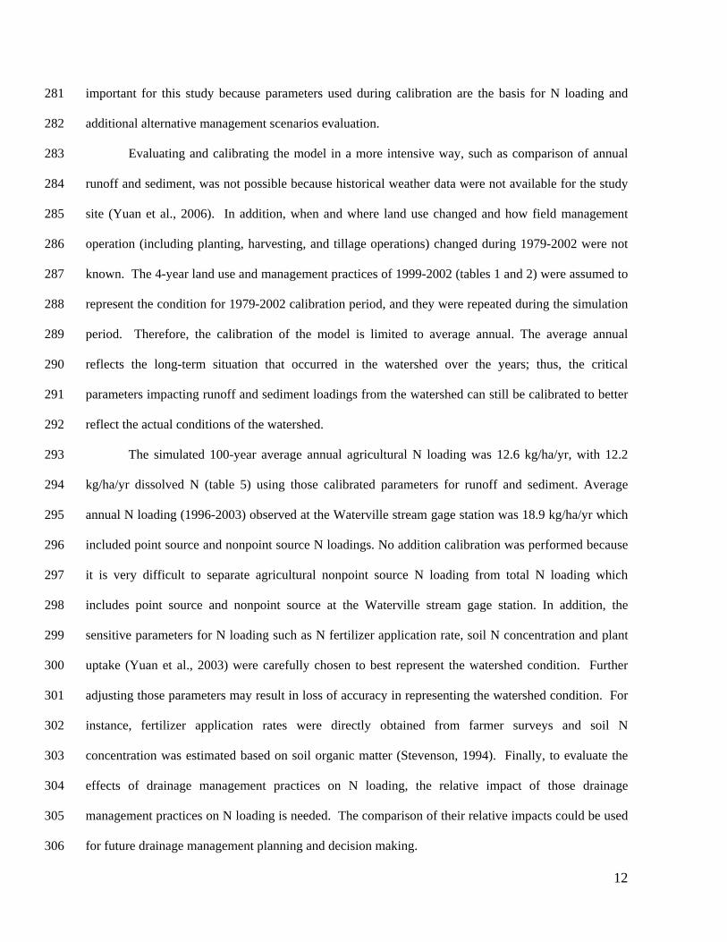
important for this study because parameters used during calibration are the basis for N loading and 281

additional alternative management scenarios evaluation. 282

Evaluating and calibrating the model in a more intensive way, such as comparison of annual 283

runoff and sediment, was not possible because historical weather data were not available for the study 284

site (Yuan et al., 2006). In addition, when and where land use changed and how field management 285

operation (including planting, harvesting, and tillage operations) changed during 1979-2002 were not 286

known. The 4-year land use and management practices of 1999-2002 (tables 1 and 2) were assumed to 287

represent the condition for 1979-2002 calibration period, and they were repeated during the simulation 288

period. Therefore, the calibration of the model is limited to average annual. The average annual 289

reflects the long-term situation that occurred in the watershed over the years; thus, the critical 290

parameters impacting runoff and sediment loadings from the watershed can still be calibrated to better 291

reflect the actual conditions of the watershed. 292

The simulated 100-year average annual agricultural N loading was 12.6 kg/ha/yr, with 12.2 293

kg/ha/yr dissolved N (table 5) using those calibrated parameters for runoff and sediment. Average 294

annual N loading (1996-2003) observed at the Waterville stream gage station was 18.9 kg/ha/yr which 295

included point source and nonpoint source N loadings. No addition calibration was performed because 296

it is very difficult to separate agricultural nonpoint source N loading from total N loading which 297

includes point source and nonpoint source at the Waterville stream gage station. In addition, the 298

sensitive parameters for N loading such as N fertilizer application rate, soil N concentration and plant 299

uptake (Yuan et al., 2003) were carefully chosen to best represent the watershed condition. Further 300

adjusting those parameters may result in loss of accuracy in representing the watershed condition. For 301

instance, fertilizer application rates were directly obtained from farmer surveys and soil N 302

concentration was estimated based on soil organic matter (Stevenson, 1994). Finally, to evaluate the 303

effects of drainage management practices on N loading, the relative impact of those drainage 304

management practices on N loading is needed. The comparison of their relative impacts could be used 305

for future drainage management planning and decision making. 306

13

EVALUATION OF ALTERNATIVE DRAINAGE MANAGEMENT PRACTICES 307

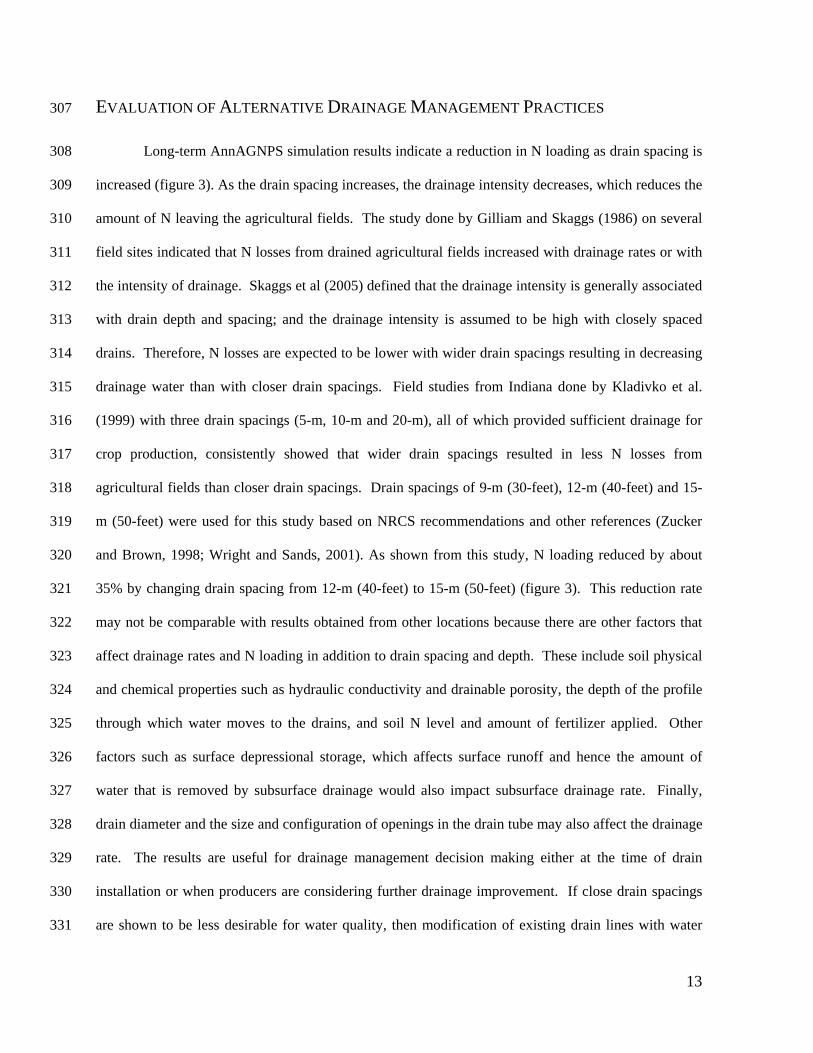
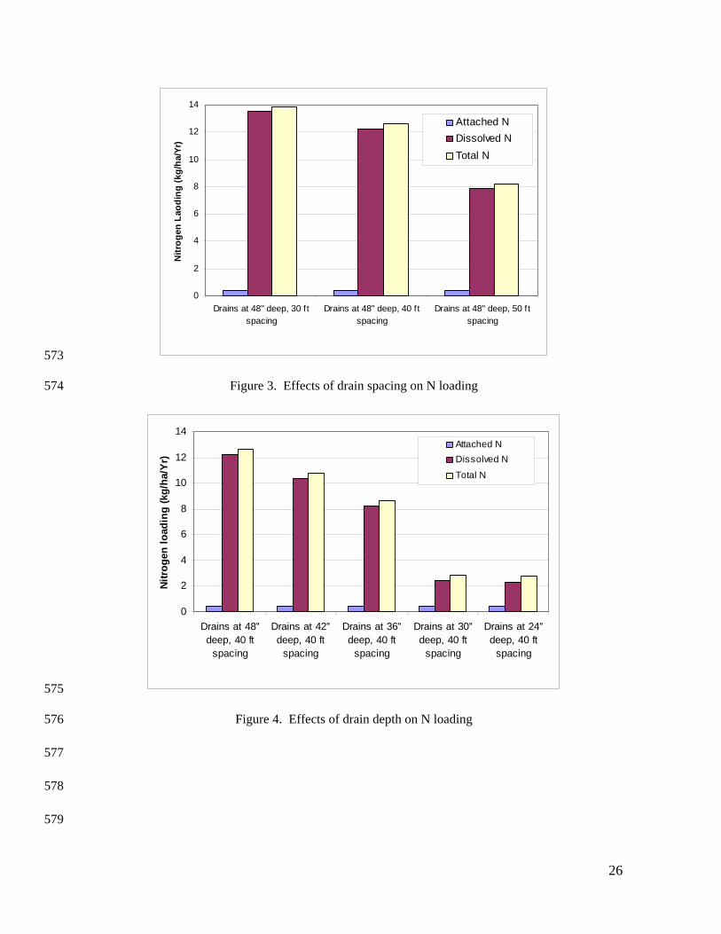
Long-term AnnAGNPS simulation results indicate a reduction in N loading as drain spacing is 308

increased (figure 3). As the drain spacing increases, the drainage intensity decreases, which reduces the 309

amount of N leaving the agricultural fields. The study done by Gilliam and Skaggs (1986) on several 310

field sites indicated that N losses from drained agricultural fields increased with drainage rates or with 311

the intensity of drainage. Skaggs et al (2005) defined that the drainage intensity is generally associated 312

with drain depth and spacing; and the drainage intensity is assumed to be high with closely spaced 313

drains. Therefore, N losses are expected to be lower with wider drain spacings resulting in decreasing 314

drainage water than with closer drain spacings. Field studies from Indiana done by Kladivko et al. 315

(1999) with three drain spacings (5-m, 10-m and 20-m), all of which provided sufficient drainage for 316

crop production, consistently showed that wider drain spacings resulted in less N losses from 317

agricultural fields than closer drain spacings. Drain spacings of 9-m (30-feet), 12-m (40-feet) and 15-318

m (50-feet) were used for this study based on NRCS recommendations and other references (Zucker 319

and Brown, 1998; Wright and Sands, 2001). As shown from this study, N loading reduced by about 320

35% by changing drain spacing from 12-m (40-feet) to 15-m (50-feet) (figure 3). This reduction rate 321

may not be comparable with results obtained from other locations because there are other factors that 322

affect drainage rates and N loading in addition to drain spacing and depth. These include soil physical 323

and chemical properties such as hydraulic conductivity and drainable porosity, the depth of the profile 324

through which water moves to the drains, and soil N level and amount of fertilizer applied. Other 325

factors such as surface depressional storage, which affects surface runoff and hence the amount of 326

water that is removed by subsurface drainage would also impact subsurface drainage rate. Finally, 327

drain diameter and the size and configuration of openings in the drain tube may also affect the drainage 328

rate. The results are useful for drainage management decision making either at the time of drain 329

installation or when producers are considering further drainage improvement. If close drain spacings 330

are shown to be less desirable for water quality, then modification of existing drain lines with water 331

14

table control structures to have some drain lines turned off might be a practical strategy to mitigate the 332

negative impacts of drainage water. 333

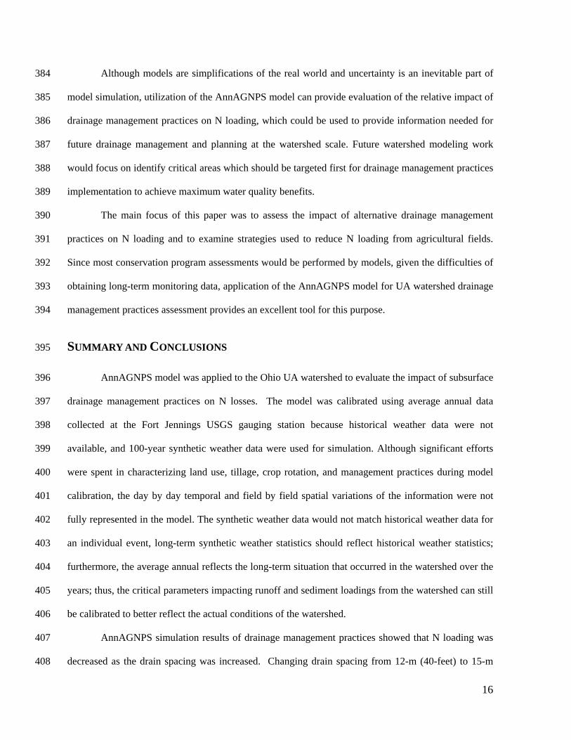
Results also showed that N loading decreased as drain depth decreased (figure 4). This is 334

because as drain depth decreased, drainage intensity decreased which resulted in less drainage water 335

leaving the agricultural fields (Skaggs et al, 2005). Less drainage water carried less N out of the 336

agricultural fields. Thus, N loadings are expected to be lower with shallower drain depth than with 337

deeper drain depth. Davis et al. (2000) used the Agricultural Drainage and Pesticide Transport 338

(ADAPT) model, a daily time step continuous water table management model, to simulate the impact 339

of fertilizer and drain spacing and depth on N losses for a Webster clay loam near Waseca, Southern 340

Minnesota. Their results showed that N losses decreased as drain depths (1.5-m, 1.2-m and 0.9-m) 341

decreased. Results from Skaggs and Chescheir (2003) with DRAINMOD simulations for a Portsmouth 342

sandy loam at Plymouth, North Carolina also showed that N losses decreased as drain depths (1.5-m, 343

1.25-m, 1.0-m and 0.75-m) decreased. ADAPT and DRAINMOD are field scale models. Depths of 344

1.2-m (48-inch), 1.1-m (42-inch), 0.9-m (36-inch), 0.8-m (30-inch), and 0.6-m (24-inch) were used in 345

this study based on the NRCS recommendation. About 15% of N was reduced by changing the drain 346

depth from 1.2-m (48-inch) to 1.1-m (42-inch) (figure 4). An additional 20% of N was reduced by 347

changing the drain depth from 1.1-m (42-inch) to 0.9-m (36-inch) (figure 4). There was only a slight 348

reduction predicted by changing the drain depth from 0.8-m (30-inch) to 0.6-m (24-inch) (figure 4). 349

Thus, drain depths shallower than 0.6-m (24-inch) were not analyzed. This reduction rate may not be 350

comparable with results obtained from other locations because there are other factors discussed 351

previously impacting drainage rate and N loading. The results on drain depths are also useful for drain 352

installation and/or further drainage improvement. If deeper drain depths are shown to be less desirable 353

for water quality, then modification of existing drain depth can be achieved with water table control 354

structures to raise water table (acting as shallow drain) according to crop growth stage. Holding water 355

in the fields will increases the time for denitrification to occur and decreases the transport on N from 356

subsurface water losses to surface waters. 357

15

Nitrogen loading could be significantly reduced by controlling water into subsurface drains 358

from November 1 to April 1 of each year based on model simulations (figure 5). This result is 359

consistent with field observations at various locations (Gilliam and Skaggs, 1986; Drury et al., 1996; 360

Ng et al., 2002; Osmond et al., 2002; Drury et al., 2009). About 64% of N was reduced by completely 361

controlling subsurface drainages (setting weirs at surface) for drain depth of 1.2-m (48-inch) when 362

compared to the conventional drainage system (free drainage from November 1 to April 1) (figure 5). 363

Similarly, 66% of N was reduced for a drain depth of 1.1-m (42-inch), and 59% for a drain depth of 364

0.9-m (36-inch) (figure 5). As shallower drains, completely controlling subsurface drains (setting weirs 365

at surface) in the dormant season also hold water in the fields which potentially increases 366

denitrification and decreases the amount of subsurface water losses to surface waters which decrease N 367

load to surface water. However, little additional impact was found by completely controlling 368

subsurface drains in the dormant season for drain depths shallower than 0.8-m (30-inch). Therefore, if 369

agricultural producers are adverse to the idea of “completely controlling subsurface drainages or 370

completely turning the drains off” at any time, setting the drainage outlet (depth of drain) at 24-inch or 371

above would achieve the goal of reducing N loading significantly without turning the drains off (figure 372

5). As indicated in figure 5, nitrogen loading does not change much by completely controlling 373

subsurface drainages in dormant season for drain depths of 30-inch and 24-inch. 374

Therefore, wider drain spacings and shallow drain depths are recommended to reduce N 375

loading from the fields. In addition, wider drain spacings and shallow drain depths also conserve 376

water. However, information on how crops react to different drainage management practices is also 377

needed to make any final decisions. Completely turning the drains off during the dormant season 378

(November 1 to April 1) appears to be an ideal and very promising approach in reducing N loading 379

because there is not much of a concern for impacting crop productivity for this practice. However, 380

shallow drains such as setting the drainage outlet (depth of drain) at 24-inch or above would achieve 381

the goal of reducing N loading significantly as completely turning the drains off during the dormant 382

season (November 1 to April 1). 383

16

Although models are simplifications of the real world and uncertainty is an inevitable part of 384

model simulation, utilization of the AnnAGNPS model can provide evaluation of the relative impact of 385

drainage management practices on N loading, which could be used to provide information needed for 386

future drainage management and planning at the watershed scale. Future watershed modeling work 387

would focus on identify critical areas which should be targeted first for drainage management practices 388

implementation to achieve maximum water quality benefits. 389

The main focus of this paper was to assess the impact of alternative drainage management 390

practices on N loading and to examine strategies used to reduce N loading from agricultural fields. 391

Since most conservation program assessments would be performed by models, given the difficulties of 392

obtaining long-term monitoring data, application of the AnnAGNPS model for UA watershed drainage 393

management practices assessment provides an excellent tool for this purpose. 394

SUMMARY AND CONCLUSIONS 395

AnnAGNPS model was applied to the Ohio UA watershed to evaluate the impact of subsurface 396

drainage management practices on N losses. The model was calibrated using average annual data 397

collected at the Fort Jennings USGS gauging station because historical weather data were not 398

available, and 100-year synthetic weather data were used for simulation. Although significant efforts 399

were spent in characterizing land use, tillage, crop rotation, and management practices during model 400

calibration, the day by day temporal and field by field spatial variations of the information were not 401

fully represented in the model. The synthetic weather data would not match historical weather data for 402

an individual event, long-term synthetic weather statistics should reflect historical weather statistics; 403

furthermore, the average annual reflects the long-term situation that occurred in the watershed over the 404

years; thus, the critical parameters impacting runoff and sediment loadings from the watershed can still 405

be calibrated to better reflect the actual conditions of the watershed. 406

AnnAGNPS simulation results of drainage management practices showed that N loading was 407

decreased as the drain spacing was increased. Changing drain spacing from 12-m (40-feet) to 15-m 408

17

(50-feet) reduced N loading by 35%. Simulation results also showed that N loading was decreased as 409

drain depth was decreased. Changing the drain depth from 1.2-m (48-inch) to 1.1-m (42-inch) reduced 410

N loading by 15%, and an additional 20% reduction can be achieved by changing the drain depth from 411

1.1-m (42-inch) to 0.9-m (36-inch). Only a slight reduction was predicted by changing the drain depth 412

from 0.8-m (30-inch) to 0.6-m (24-inch). Furthermore, N loading could be significantly reduced by 413

controlling subsurface drains from November 1 to April 1 of each year. Up to 66% of N can be 414

reduced by completely controlling subsurface drainages depending on drain depths. These results are 415

useful for future drainage management and planning at the watershed scale. Although findings from 416

this study are consistent with field observations at other locations, but the actual reductions rates 417

obtained from this study may not be comparable with results obtained from other locations because 418

there are other factors impacting N loading. Future watershed modeling work would focus on targeting 419

critical areas for drainage management practices implementation to achieve maximum water quality 420

benefits. 421

Notice: Although this work was reviewed by USEPA and approved for publication, it may not 422

necessarily reflect official Agency policy. Mention of trade names or commercial products does not 423

constitute endorsement or recommendation for use. 424

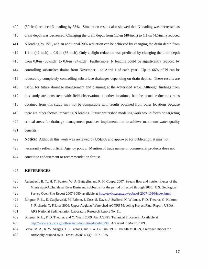
REFERENCES 425

Aulenbach, B. T., H. T. Buxton, W. A. Battaglin, and R. H. Coupe. 2007. Stream flow and nutrient fluxes of the 426 Mississippi-Atchafalaya River Basin and subbasins for the period of record through 2005. U.S. Geological 427

Survey Open-File Report 2007-1080, available at http://toxics.usgs.gov/pubs/of-2007-1080/index.html. 428 Bingner, R. L., K. Czajkowski, M. Palmer, J. Coss, S. Davis, J. Stafford, N. Widman, F. D. Theurer, G. Koltum, 429

P. Richards, T. Friona. 2006. Upper Auglaize Watershed AGNPS Modeling Project Final Report. USDA-430 ARS National Sedimentation Laboratory Research Report No. 51. 431

Bingner, R. L., F. D. Theurer, and Y. Yuan. 2009. AnnAGNPS Technical Processes. Available at 432 http://www.ars.usda.gov/Research/docs.htm?docid=5199. Accessed in March 2009. 433

Breve, M. A., R. W. Skaggs, J. E. Parsons, and J. W. Gilliam. 1997. DRAINMOD-N, a nitrogen model for 434 artificially drained soils. Trans. ASAE 40(4): 1067-1075. 435

18

Chung, S. O., A. D. Ward, N. R. Fausey, and T. J. Logan. 1991. Evaluation of the pesticide component of the 436 ADAPT water table management model. Paper no. 91-2632. ASAE Winter Meeting, Chicago, IL. Dec. 16-437 17, 1991. ASAE, St. Hoseph, MI. 438

Chung, S. O., A. D. Ward, and C. W. Schalk. 1992. Evaluation of the hydrologic component of the ADAPT 439 water table management model. Trans. ASAE 35(2): 571-579. 440

Crumpton, W. G., G. A. Stenback, B. A. Miller, and M. J. Helmers. 2007. Potential Benefits of Wetland Filters 441 for Tile Drainage System: Impact on Nitrate Loads to Mississippi River Subbasins. Washington, DC: 442 USDA. 443

Davis, D. M., P. H. Gowda, D. J. Mulla, and G. W. Randall. 2000. Modeling nitrate nitrogen leaching in 444 response to nitrogen fertilizer rate and tile depth or spacing for southern Minnesota, USA. J. Environ. Qual. 445 29(5): 1568-1581. 446

Desmond, E. D., A. D. Ward, N. R. Fausey, and T. J. Logan. 1995. Nutrient component evaluation of the 447 ADAPT water management model. P 21-30. in proceedings of the Int. Symp. On Water Quality Modeling, 448 Orlando, FL., April 2-5, 1995. ASAE, St. Hoseph, MI. 449

Dinnes, D. L., D. L. Karlen, D. B. Jaynes, T. C. Kaspar, J. L. Hatfield, T. S. Colvin, and C. A. Cambardella. 450 2002. Nitrogen management strategies to reduce nitrate leaching in tile drained Midwestern soils. Agron. J. 451 94(1): 153-171. 452

Drury, C. F., C. S. Tan, J. D. Gaynor, T. O. Oloya, and T. W. Welacky. 1996. Influence of controlled drainage-453 subirrigation on surface and tile drainage nitrate loss. J. of Environ. Qual. 25(2): 317-324. 454

Drury, C. F., C. S. Tan, W. D. Reynolds, T. W. Welacky, T. O. Oloya, and J. D. Gaynor. 2009. Managing Tile 455 Drainage, Subirrigation, and Nitrogen Fertilization to Enhance Crop Yields and Reduce Nitrate Loss. J. of 456 Environ. Qual. 38(3): 1193-1204. 457

Evans, R. O., and R. W. Skaggs. 1989. Design guidelines for water table management systems on Coastal Plain 458 soils. Applied Engineering in Agriculture 5(4): 539-548. 459

Evans, R. O., J. W. Gilliam, and R. W. Skaggs. 1995. Controlled versus conventional drainage effects on water 460 quality. J. Irr. & Drain. 121(4): 271-276. 461

Freeze, R. A., and J. A. Cherry. 1979. Groundwater. Prentice Hall, Englewood Cliffs, N. J.: 07632. 462 Gilliam, J. W., R. W. Skaggs, and S. B. Weed. 1979. Drainage control to diminish nitrate loss from agricultural 463

fields. J. Environ. Qual. 8: 137-142. 464 Gilliam, J. W., and R. W. Skaggs. 1986. Controlled agricultural drainage to maintain water quality. J. Irrig. 465

Drain. Eng. 112(3): 254-263. 466 Gilliam, J. W., J. L. Baker, and K. R. Reddy. 1999. Water quality effects of drainage in humid regions. In 467

Agricultural Drainage, 801-830. R. W. Skaggs and J. van Schilfgaarde, eds. Madison, Wisc.: SSSA. 468 Johnson, G. L., C. L. Hanson, S. P. Hardegree, and E. B. Ballard. 1996. Stochastic weather simulation: Overview 469

and analysis of two commonly used models. J. Applied Meteorology 35(10): 1878-1896. 470 Johnson, G. L., C. Daly, G. H. Taylor, and C. L. Hanson. 2000. Spatial variability and interpolation of stochastic 471

weather simulation model parameters. J. Applied Meteorology 39(1): 778-796. 472

19

Johnson, W. E. 1990. Ecological problems associated with agricultural development: some examples in the 473 United States. In Ecological Risks: Perspectives from Poland and the United States. Edited by Grodzinski, 474 W., E. B. Cowling, A. I. Breymeyer, A. S. Phillips, S. I. Auerbach, A. M. Bartuska, M. A. Harwell. National 475 Academy Press, Washington D. C. 476

Kalita, P. K, R. A. C. Cooke, S. M. Anderson, M. C. Hirschi, and J. K. Mitchell. 2007. Subsurface drainage and 477 water quality: The Illinois experience. Trans. ASABE 50(5): 1651-1656. 478

Kladivko, E. J., J. Rrochulska, R. R. Turco, G. E. Van Scoyoc, and J. D. Eigel. 1999. Pesticide and nitrate 479 transport into subsurface tile drains of different spacings. J. Environ. Qual. 28(3): 997-1004. 480

Luo, W. 1999. Modification and testing of DRAINMOD for freezing, thawing, and snowmelt. PhD diss. Raleigh, 481 N.C.: North Carolina State University. 482

Mitchell, J. K. G. F. McIsaac, S. E. Walker, and M. C. Hirschi. 2000. Nitrate in river and subsurface flows from 483 an east central Illinois watershed. Trans. ASAE 43(2): 337-42. 484

Mitsch, W. J., J. W. Day, Jr., J. W. Gilliam, P. M. Groffman, D. L. Hey, G. W. Randall, and N. Wang. 2001. 485 Reducing nitrogen loading to the Gulf of Mexico from the Mississippi River Basin: Strategies to counter a 486 persistent ecological problem. BioScience 51(5): 373-388. 487

Natural Resources Conservation Service (NRCS). 2009. Soil Survey Geographic (SSURGO) Database, 488 Available at: http://www.soils.usda.gov/survey/geography/ssurgo/. Accessed in January 2009. 489

Ng, H. Y. F., C. S. Tan, C. F. Drury, and J. D. Gaynor. 2002. Controlled drainage and subirrigation influences 490 tile nitrate loss and corn yields in a sandy loam soil in Southwestern Ontario. Agriculture Ecosystems & 491 Environment 90(1): 81-88. 492

Ohio EPA, 2008. Lake Erie: Lakewide management plan. Available at 493 http://www.epa.ohio.gov/dsw/ohiolamp/index.aspx. Accessed on September 15, 2009. 494

Osmond, D. L., J. W. Gilliam, and R. O. Evans. 2002. Riparian Buffers and Controlled Drainage to Reduce 495 Agricultural Nonpoint Source Pollution, North Carolina Agricultural Research Service Technical Bulletin 496 318, North Carolina State University, Raleigh, NC. 497

Rabalais, N. N., R. E. Turner, D. Justic, Q. Dortch, J. W. Wiseman, Jr., and B. K. Sen Gupta. 1996. Nutrient 498 changes in the Mississippi River and system response on the adjacent continental shelf. Estuaries 19(2B): 499 385-407. 500

Rabalais, N. N., R. E. Turner, D. Justic, Q. Dortch, and W. J. Wiseman. 1999. Characterization of hypoxia: Topic 501 1 report for the integrated assessment on hypoxia in the Gulf of Mexico. Decision Analysis Series No. 15. 502 Silver Spring, Md.: NOAA Coastal Office. 503

Renard, K. G., G. R. Foster, G. A. Weesies, D. K. McCool, and D. C. Yoder, coordinators. 1997. Predicting Soil 504 Erosion by Water: A Guide to Conservation Planning with the Revised Universal Soil Loss Equation 505 (RUSLE). USDA Agriculture Handbook No. 703. 506

Sands, G. R., I. Song, L. M. Busman, and B. Hansen. 2008. The effects of subsurface drainage depth and 507 intensity on nitrate loads in the northern cornbelt. Trans. ASABE 51 (3): 937-946. 508

20

Skaggs, R. W., and G. M. Chescheir, III. 2003. Effects of subsurface drain depth on nitrogen losses from drained 509 lands. Trans. ASAE 46(2): 237-244. 510

Skaggs, R. W., M. A. Youssef, G. M. Chescheir, and J. W. Gilliam. 2005. Effects of drainage intensity on 511 nitrogen losses from drained lands. Trans. ASABE 48(6): 2169-2177. 512

Smedema L. K., and D. W. Rycroft, 1983. Land Drainage. Cornell University Press, Ithaca, New York. 513 Soil Conservation Service (SCS). 1985. National Engineering Handbook. Section 4: Hydrology. U.S. 514

Department of Agriculture, Washington D.C. 515 Stevenson, F. J. 1994. Humus Chemistry: Genesis, Composition, Reactions. John Wiley & Sons, Inc., New 516

York, NY. 517 U. S. Environmental Protection Agency Science Advisory Board, 2007. Hypoxia in the Northern Gulf of 518

Mexico: An Update by the EPA Science Advisory Board. Washington, D.C. Available at 519 http://www.epa.gov/msbasin/pdf/sab_report_2007.pdf. Accessed on September 10, 2009. 520

U. S. Environmental Protection Agency. 2008. Maximum Contaminant Levels (subpart B of 141, National 521 primary drinking water regulations). In U.S. Code of Federal Regulations, Title 40, Parts 100-149: 559-563. 522 Washington, D.C.: GPO. 523

Wright, J., and G. Sands. 2001. Planning an agricultural subsurface drainage system. Agricultural Drainage 524 publication series. The University of Minnesota. Available at: 525 http://www.extension.umn.edu/distribution/cropsystems/components/07685.pdf. Accessed on August 31, 526 2010. 527

Young, R. A., C. A. Onstad, D. D. Bosch, and W. P. Anderson. 1989. AGNPS: A nonpoint-source pollution 528 model for evaluating agricultural watersheds. Journal of Soil and Water Conservation 44(2):168-173. 529

Yuan, Y., R. L. Bingner, and R. A. Rebich. 2003. Evaluation of AnnAGNPS nitrogen loading in an agricultural 530 watershed. Journal of AWRA 39(2): 457-466. 531

Yuan, Y., R. L. Bingner, and F. D. Theurer. 2006. Subsurface flow component for AnnAGNPS. Applied 532 Engineering in Agriculture 22(2): 231-241. 533

Yuan, Y., R. L. Bingner, and F. D. Theurer. 2008. AnnAGNPS: Baseflow feature. Paper No. 08-4143, ASABE, 534 St. Joseph, MI. 535

Zhao, S., S. C. Gupta, D. R. Higgins, and J. F. Moncrief. 2000. Predicting subsurface drainage, corn yield, and 536 nitrate-N losses with DRAINMOD-N. Journal of Environ. Qual. 29(3): 817-825. 537

Zucker, L. A., and L. C. Brown. 1998. Agricultural Drainage: Water quality impacts and subsurface drainage 538 studies in the Midwest. Ohio State University Extension Bulletin 871. The Ohio State University. available 539 at http://ohioline.osu.edu/b871/index.html. Accessed on August 31, 2010. 540

541

21

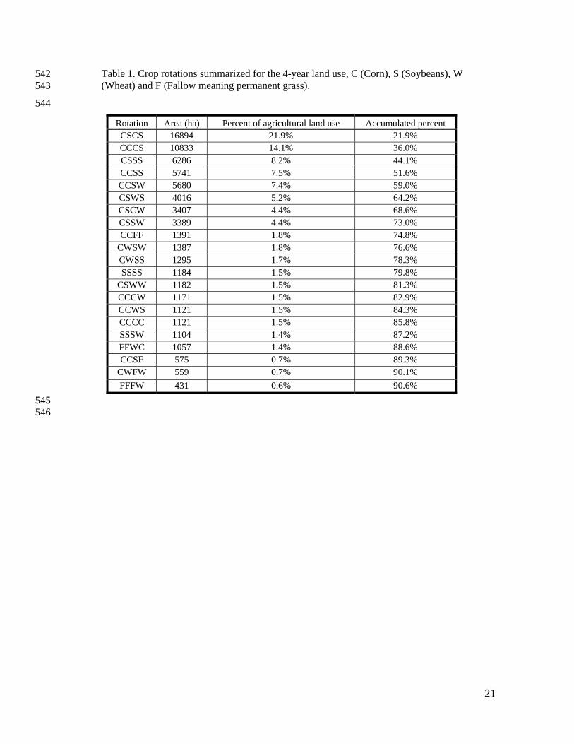
Table 1. Crop rotations summarized for the 4-year land use, C (Corn), S (Soybeans), W 542 (Wheat) and F (Fallow meaning permanent grass). 543

544

Rotation Area (ha) Percent of agricultural land use Accumulated percent CSCS 16894 21.9% 21.9% CCCS 10833 14.1% 36.0% CSSS 6286 8.2% 44.1% CCSS 5741 7.5% 51.6% CCSW 5680 7.4% 59.0% CSWS 4016 5.2% 64.2% CSCW 3407 4.4% 68.6% CSSW 3389 4.4% 73.0% CCFF 1391 1.8% 74.8%

CWSW 1387 1.8% 76.6% CWSS 1295 1.7% 78.3% SSSS 1184 1.5% 79.8%

CSWW 1182 1.5% 81.3% CCCW 1171 1.5% 82.9% CCWS 1121 1.5% 84.3% CCCC 1121 1.5% 85.8% SSSW 1104 1.4% 87.2% FFWC 1057 1.4% 88.6% CCSF 575 0.7% 89.3%

CWFW 559 0.7% 90.1% FFFW 431 0.6% 90.6%

545 546

22

Table 2. Upper Auglaize watershed 4-year crop, tillage, and land-use distribution in percent, the total 547 area is 85,812 hectares. 548

Landuse Tillage 1999 2000 2001 2002

Corn

Conventional 10.1% 13.1% 10.5% 10.5% Mulch till 18.7% 17.0% 20.3% 17.9% No till 10.4% 14.1% 12.2% 14.0% Total 39.3% 44.2% 43.0% 42.3%

Beans

Conventional 8.7% 6.0% 7.4% 9.4% Mulch till 9.6% 16.8% 11.5% 13.7% No till 11.8% 11.1% 13.7% 11.2% Total 30.0% 33.9% 32.5% 34.2%

Wheat

Conventional 1.9% 2.6% 3.7% 1.6% Mulch till 5.3% 3.8% 4.3% 2.7% No till 5.2% 4.6% 3.1% 3.8% Total 12.4% 10.9% 11.1% 8.0%

Grass

Conventional 1.4% 0.4% 0.5% 0.6% Mulch till 4.2% 0.2% 1.7% 3.7% No till 2.7% 0.4% 1.1% 1.2% Continuous 0.4% 0.4% 0.4% 0.4% Total 8.7% 1.4% 3.7% 5.8%

Forest 5.6% 5.6% 5.6% 5.6% Residential 2.0% 2.0% 2.0% 2.0% Roads 1.4% 1.4% 1.4% 1.4% Commercial 0.5% 0.5% 0.5% 0.5% Water 0.1% 0.1% 0.1% 0.1% Grand Total 100.0% 100.0% 100.0% 100.0%

549

Table 3. Fertilizer application for various crops. 550

Crop Type Nitrogen (kg./ha..) P2O5 (kg./ha.)

Corn 157 50

Soybean 0 34

Wheat 65 45

Alfalfa 0 73

551 552 553

23

Table 4. Curve numbers used for model simulations after calibration 554

AnnAGNPS land cover

Land cover class from table 9 of the NHD-4 (NRCS, 1985)

Curve Number

Hydrological soil group

A B C D

Row crop with NT* Row crop contoured and terraced (good) 62 71 78 81

Row crop with RT* Row crop contoured with crop residue (good) 64 74 81 85

Row crop with CT* Row crop straight row (poor) 72 81 88 91

Small grain with NT* Small grain contoured and terraced (good) 59 70 78 81

Small grain with RT* Small grain contoured and terraced (good) 60 72 80 84

Small grain with CT* Small grain contoured and terraced (good) 64 75 83 86

Fallow Fallow with crop residue (good) 74 83 88 90

Forest Woods (good) 30 55 70 77

Commercial Residential (38% impervious) 61 75 83 87

Residential Residential (38% impervious) 61 75 83 87

Roads Roads (paved w/ditch) 83 89 92 93 * NT refers to no-tillage, RT refers to reduced tillage and CT refers to conventional tillage. 555

556 Table 5. Calibration outputs of runoff sediment and nitrogen as compared to observed values for 557

existing watershed conditions. 558 559

Item AnnAGNPS Simulation USGS Observation

Watershed annual average direct surface runoff (mm) 162.6

Watershed annual average subsurface flow (mm) 91.4

Watershed annual average total runoff (mm) 254.0 254.0

Sediment loading at the watershed outlet (t/ha/Yr) 0.771 0.753

Total N loading at the Waterville gage (kg/ha/Yr) 12.6 18.9

560

561

562

563

564

24

565

Figure 1. AnnAGNPS input data sections 566

25

567

Figure 2. The Maumee River basin drainage network, Upper Auglaize watershed, and the Wapakoneta 568

and Fort Jennings Gage Stations. 569

570

571

572

MichiganOhio

IndianaIn

dian

a

Ohi

o

Michigan LakeErie

#

Toledo

#

WatervilleStream Gage

#

Ft. JenningsStream Gage

#Defiance

Upper Auglaize Project AreaMaumee River Basin

N

EW

S

16 0 16 Miles

Streams

Upper Auglaize Project Area

State Boundaries

Maumee Basin

County Boundaries

LEGEND

Ohio NRCS GIS 4/14/2004

#

Ft. Wayne

#

Wapakoneta

26

0

2

4

6

8

10

12

14

Drains at 48'' deep, 30 ftspacing

Drains at 48'' deep, 40 ftspacing

Drains at 48'' deep, 50 ftspacing

Nitr

ogen

Lao

ding

(kg/

ha/Y

r)

Attached NDissolved NTotal N

573

Figure 3. Effects of drain spacing on N loading 574

0

2

4

6

8

10

12

14

Drains at 48''deep, 40 ft

spacing

Drains at 42''deep, 40 ft

spacing

Drains at 36''deep, 40 ft

spacing

Drains at 30''deep, 40 ft

spacing

Drains at 24''deep, 40 ft

spacing

Nitr

ogen

load

ing

(kg/

ha/Y

r)

Attached NDissolved N

Total N

575

Figure 4. Effects of drain depth on N loading 576

577

578

579

27

0

2

4

6

8

10

12

14

Drains at 48''deep

Drains off11/1/ to 4/1,

48'' deep

Drains at 42''deep

Drains off11/1/ to 4/1,

42'' deep

Drains at 36''deep

Drains off11/1/ to 4/1,

36'' deep

Drains at 30''deep

Drains off11/1/ to 4/1,

30'' deep

Drains at 24''deep

Drains off11/1/ to 4/1,

24'' deep

Alternatives

Nitr

ogen

load

ing

(kg/

ha/Y

r)Attached N

Dissolved N

Total N

580

Figure 5. Effects of turning drains off during dormant season (Nov. 1 to Apr. 1) on N loading 581