AFRL-RW-EG-TR-2011-167

A A THREE DIMENSIONAL EULERIAN CODE FOR SIMULATION OF HIGH-SPEED MULTIMATERIAL INTERACTIONS

H.S. UDAYKUMAR UNIVERSITY OF IOWA 105 JESSUP HALL IOWA CITY, IA 52241-1316 Grant No. FA8651-06-1-0002 August 2011 FINAL REPORT

AIR FORCE RESEARCH LABORATORY MUNITIONS DIRECTORATE

Air Force Materiel Command United States Air Force Eglin Air Force Base, FL 32542

DISTRIBUTION A. Approved for public release, distribution unlimited. 96th ABW/PA Approval and Clearance # 96ABW-2012-0022 dated 25 January 2012.

DEPARTMENT OF THE AIR FORCE AIR FORCE RESEARCH LABORATORY (AFMC)

EGLIN AIR FORCE BASE, FLORIDA

MEMORANDUM FOR AFRL/RW CA-N FROM: AFRL/RWWC SUBJECT: Request for Review and Clearance 1. Request review and approval of the attached technical report for public release. a. TITLE OF PUBLICATION: A Three-Dimensional Eulerian Code for Simulation of High-Speed

Multimaterial Interactions b. AUTHOR: H.S. Udaykumar c. TITLE OF JOURNAL: NA d. SPONSOR: NA

e. CLASSIFICATION: Unclassified f. FOREIGN NATIONALS WILL HAVE ACCESS TO THE IMAGES AFTER THEY ARE

CLEARED FOR RELEASE BY PUBLIC AFFAIRS. g. The technical report WILL be published in the open literature. h. Deadline: ASAP i. JON: 25020734

2. The material contained in the attached technical report is technically accurate, unclassified, and suitable for public release. 3. Even though key words that appear in the technical presentation are included in the RW OPSEC Critical Information List (RW OPSEC CIL), RW Technology Protection Plan Critical Research Technology List ( RW TPPCRTL), U.S. Munitions List (USML) (International Traffic in Arms Regulation (ITAR), 22 Code of Federal Regulations (CFR), Part 121), Militarily Critical Technologies List (MCTL), and the Commerce Control List (CCL), (Export Administration Regulations (EAR), 15 CFR, Part 774, Categories 0-9), the particular aspect of technology that the abstract addresses is not included as part of the RW OPSEC CIL, RW TPPCRTL, USML, MCTL, and/or the CCL, does not meet the definition of Critical Technology as defined by DoDD 5230.25, and will not result in the transfer of any militarily critical technology. 4. If you have any questions please contact Dr. Michael E Nixon AFRL/RWWC, 883-2656. ORIGINAL SIGNED

Dr. Craig Ewing CTC Lead Weapon Engagement Division

Attachment: Technical Report: A Three-Dimensional Eulerian Code for Simulation of High-Speed

Multimaterial Interactions

Standard Form 298 (Rev. 8/98)

REPORT DOCUMENTATION PAGE

Prescribed by ANSI Std. Z39.18

Form Approved OMB No. 0704-0188

The public reporting burden for this collection of information is estimated to average 1 hour per response, including the time for reviewing instructions, searching existing data sources, gathering and maintaining the data needed, and completing and reviewing the collection of information. Send comments regarding this burden estimate or any other aspect of this collection of information, including suggestions for reducing the burden, to Department of Defense, Washington Headquarters Services, Directorate for Information Operations and Reports (0704-0188), 1215 Jefferson Davis Highway, Suite 1204, Arlington, VA 22202-4302. Respondents should be aware that notwithstanding any other provision of law, no person shall be subject to any penalty for failing to comply with a collection of information if it does not display a currently valid OMB control number. PLEASE DO NOT RETURN YOUR FORM TO THE ABOVE ADDRESS. 1. REPORT DATE (DD-MM-YYYY) 2. REPORT TYPE 3. DATES COVERED (From - To)

4. TITLE AND SUBTITLE 5a. CONTRACT NUMBER

5b. GRANT NUMBER

5c. PROGRAM ELEMENT NUMBER

5d. PROJECT NUMBER

5e. TASK NUMBER

5f. WORK UNIT NUMBER

6. AUTHOR(S)

7. PERFORMING ORGANIZATION NAME(S) AND ADDRESS(ES) 8. PERFORMING ORGANIZATION REPORT NUMBER

9. SPONSORING/MONITORING AGENCY NAME(S) AND ADDRESS(ES) 10. SPONSOR/MONITOR'S ACRONYM(S)

11. SPONSOR/MONITOR'S REPORT NUMBER(S)

12. DISTRIBUTION/AVAILABILITY STATEMENT

13. SUPPLEMENTARY NOTES

14. ABSTRACT

15. SUBJECT TERMS

16. SECURITY CLASSIFICATION OF: a. REPORT b. ABSTRACT c. THIS PAGE

17. LIMITATION OF ABSTRACT

18. NUMBER OF PAGES

19a. NAME OF RESPONSIBLE PERSON

19b. TELEPHONE NUMBER (Include area code)

DISTRIBUTION A

NOTICE AND SIGNATURE PAGE

Using Government drawings, specifications, or other data included in this document for any purpose other than Government procurement does not in any obligate the U.S. Government. The fact that the Government formulated or supplied the drawings, specifications, or other data does not license the holder or any other person or corporation, or convey any rights or permission to manufacture, use, or sell any patented invention that may relate to them. This report was cleared for public release by the 96th Air Base Wing, Public Affairs Office, and is available to the general public, including foreign nationals. Copies may be obtained from the Defense Technical Information Center (DTIC) < http://www.dtic.mil/dtic/index/html>. AFRL-RW-EG-TR-2011-167 HAS BEEN REVIEWED AND IS APPROVED FOR PUBLICATION IN ACCORDANCE WITH ASSIGNED DISTRIBUTION STATEMENT. FOR THE DIRECTOR: ORIGINAL SIGNED ORIGINAL SIGNED ______________________________________ _____________________________________ Dr. Craig Ewing Michael E Nixon, PhD CTC Lead Program Manager Weapon Engagement Division Computational Mechanics Branch This report is published in the interest of scientific and technical information exchange, and its publication does not constitute the Government’s approval or disapproval of its ideas or findings.

DISTRIBUTION A

A THREE-DIMENSIONAL EULERIAN CODE FOR SIMULATION OF HIGH-SPEED MULTIMATERIAL

INTERACTIONS

PI: H. S. UDAYKUMAR

PROFESSOR, MECHANICAL AND INDUSTRIAL ENGINEERING, THE UNIVERSITY OF IOWA, IOWA CITY

AUGUST 2011

ii

DISTRIBUTION A

CONTENTS

Abstract.......................................................................................................................................................................... 1

1 Introduction ................................................................................................................................................................ 2

2 Governing Equations and Material Models ................................................................................................................ 3

2.1 Governing Equations .......................................................................................................................................... 3

2.2 Material Models .................................................................................................................................................. 4

3 Tracking of Embedded Interfaces .............................................................................................................................. 5

3.1 Implicit Interface Representation Using Level sets ............................................................................................ 5

3.2 Detecting and resolving collisions ...................................................................................................................... 6

4 Methodology for Ghost Fluid Treatment for Elasto-Plastic Material Interactions ..................................................... 7

4.1 Classification of the Interface and the Associated Boundary Conditions ............................................................ 7

4.2 Obtaining the value at the reflected node IP1: .................................................................................................. 11

5 Local Mesh Refinement ............................................................................................................................................ 15

6 Methodology for Parallelization ............................................................................................................................... 15

6.1 Issues with parallelizing the sharp-interface levelset-based approach ............................................................... 17

6.1.1 Handling of Global Data ............................................................................................................................. 17

6.1.2 Definition and Construction of Ghost Layer............................................................................................... 18

6.1.3 Moving Boundary Problems ..................................................................................................................... 19

6.1.4 GFM at processor boundaries ..................................................................................................................... 22

7 Methodology for Multi-Scale Modeling Using ANN ............................................................................................... 22

7.1 Numerics and methods ..................................................................................................................................... 25

7.2 Artificial Neural Network .................................................................................................................................. 28

8 Validation and Results ............................................................................................................................................ 29

8.1 Results for Axis-symmetric problems ............................................................................................................... 29

8.1.1 IMPACT of a Copper Rod over a Rigid Substrate - Axisymmetric Taylor Bar Experiment ...................... 29

8.1.2 2D Axisymmetric Penetration of Steel Target by WHA Long Rod .......................................................... 35

8.1.3 Shock Wave Interaction with Hemispherical Groove ................................................................................ 45

iii

DISTRIBUTION A

8.1.4 Perforation of Aluminum Plates by Conical-Nosed Projectile ................................................................... 48

8.1.5 Axisymmetric Dynamic-Tensile Large-Strain Impact-Extrusion of Copper .............................................. 50

8.2 Handling of fragments in case of severe plastic deformation ........................................................................... 54

8.3 Validation of parallel algorithm ......................................................................................................................... 58

8.3.1 Axisymmetric Taylor bar test at 227 m/s .................................................................................................... 58

8.4 Three Dimensional Results ................................................................................................................................ 58

8.4.1 Taylor Bar Impact ....................................................................................................................................... 59

8.4.2 Perforation and ricochet phenomenon in thin plates ................................................................................... 64

8.4.3 Fragmentation of a thin plate ...................................................................................................................... 69

8.5 Results for Multi-Scale Modeling Using ANN.................................................................................................. 70

8.5.1 Validation of the flow solver ...................................................................................................................... 71

8.5.2 Examples of ANN learning process ............................................................................................................ 71

8.5.3 Macro-scale calculations............................................................................................................................. 78

9 Conclusions ............................................................................................................................................................. 84

10 Acknowledgements ............................................................................................................................................... 84

APPENDIX ................................................................................................................................................................. 84

A.1 Governing Equations ........................................................................................................................................ 84

A.2 Equation of State (E.O.S)................................................................................................................................. 85

A.3 Constitutive Relations ....................................................................................................................................... 87

A.4 Radial Return Mapping Algorithm .................................................................................................................. 89

REFERENCES ............................................................................................................................................................ 92

1

DISTRIBUTION A

ABSTRACT

High speed material interactions may lead to large deformations followed by fragmentation. To simulate such problems in the Eulerian framework on a fixed Cartesian mesh, all interfaces (free surfaces as well as interacting material interfaces) are tracked as levelsets; to resolve shocks and interfaces, a quad-tree adaptive mesh is employed. Collisions between embedded objects are resolved using an efficient collision detection algorithm and appropriate ineterfacial conditions are supplied. This paper addresses issues associated with the treatment of all interfaces as sharp entities by defining ghost fields on each side of the interface. Key issues of supplying interfacial conditions at the location of the interface and populating the ghost cells with physically consistent values during and beyond fragmentation events are addressed. An efficient parallel algorithm is used to handle computationally intensive three-dimensional problems. Numerous examples pertaining to impact, penetration, void collapse and fragmentation phenomena are presented along with careful benchmarking to establish the validity, the accuracy and the versatility of the approach. The methodology is combined with artificial neural network technology to develop a multiscale computational framework. Detailed and highly resolved simulations are performed in subdomains where the meso-scale structure of the material is treated explicitly. The ANN is trained using the meso-scale simulations and the information gathered from these snapshot simulations is transmitted through the ANN to macro-scale simulations thereby circumventing closure problems. The techniques and results for such multi-scale simulations are also described in the report.

2

DISTRIBUTION A

1 INTRODUCTION

The phenomena of high speed impact and penetration arise in many applications including munition-target interactions[1, 2], geological impact dynamics [3, 4], shock-processing of powders [5, 6], formation of shaped charges [7, 8], etc. The hydrodynamic pressures realized in such problems are often much greater than the strength of the material and lead to short transients of elastic deformation followed by drastic plastic flow of the material. The stress and strain fields are subject to nonlinear elasto-plastic yield behavior, the models for which must be included in the governing equations . Wave propagation in the interacting media is highly nonlinear and may result in localized phenomena such as shear bands, crack propagation, fracture and/or complete failure of the material.

The fundamental challenges to a simulation capability designed to solve problems involving the physical phenomena listed above arise from the large deformations realized at high strain-rate conditions . Traditionally, the tools that have been used to solve such large deformation, transient problems have been called hydrocodes . The broad range of available hydrocodes has been reviewed by Anderson[1] and Benson . Hydrocodes may be either based on a Lagrangian formulation, such as in EPIC and DYNA, where a moving unstructured mesh is used to follow the deformation, or an Eulerian formulation, such as in CTH, where a fixed mesh is used and the boundaries are tracked through the mesh . An intermediate approach, ALE (Arbitrary Lagrangian Eulerian) , permits the mesh to move so as to conform to the contours of the deforming object, but the mesh is not necessarily attached to material points . In the Lagrangian moving mesh methods, considerable complexity is enjoined by the need for mesh management [2], to accommodate the large distortion of the embedded boundary. Therefore periodic re-meshing operations are required so that an adequately refined mesh with good mesh quality is maintained. In some cases, it is advantageous to use meshless methods such as Smooth-Particle Hydrodynamics (SPH) to cope with severe deformations .

Both Lagrangian and Eulerian frameworks have been identified with certain issues and take different paths in formulating large deformation problems in elasto-plastically deforming materials[15, 16]. Lagrangian methods adopt a multiplicative decomposition of deformation gradients and a hyperelastic model for the elastic deformation [39]. Due to the presumed existence of a mapping to the undeformed state through the flow process, they operate on the Piola-Kirchhoff stress tensor. For the large deformation cases of interest in this paper Xiao et al. point that the multiplicative model assumes the presence of an “intermediate” configuration which can be mapped on to the original undeformed state. However, such an intermediate configuration may not satisfy geometric compatibility. Furthermore, it is not clear how a mapping to the original geometry is relevant following fragmentation. The Eulerian methodology is typically based on an additive decomposition of the strain rate tensor. In terms of constitutive laws, the elastic part of deformation is governed by hypoelasticity in the Eulerian framework. There is an issue of non-integrability in the hypoelastic model which results in elastic dissipation by not fully recovering the elastic part of strain; however, in simulations involving high speed impact and penetration elastic strains are rather negligible and of little interest when compared to the plastic strain. Another concern with Eulerian formulations is with regard to oscillatory solutions for a simple shear problem; but has been shown to be resolved by using the Jaumann rate . Despite these issues, the use of true stress state using Cauchy stress tensor, handling of contact and penetration using embedded interfaces and simplicity accruing from use of a fixed global grid makes Eulerian methods very attractive and promising. However, an intrinsic limitation of adopting a fixed global grid is that local small-scale features cannot typically be adequately resolved without demanding global refinement; to circumvent this problem local adaptivity is necessary, which engenders a significant transformation of an Eulerian solver.

In this work, a sharp interface Cartesian grid-based hydrocode is developed to solve high speed impact, collision,penetration and fragmentation problems. There are two main objectives; first, calculations are to be followed past complete fragmentation while still maintaining sharp interfaces, and second, resolution should be directed to spatial and temporal localized events. Both of these demands present rather stiff challenges. In contrast to

3

DISTRIBUTION A

the previous Cartesian grid approaches [9, 10], the present effort advancing computational schemes for high-speed multimaterial interaction problems in the following ways:

1. The interfaces are tracked and represented via the traditional level set approach as opposed to the hybrid particle level set technique employed in or the marker particles approach employed in . This improves the efficiency of the calculations, obviating search procedures associated with the latter approach on the unstructured mesh in the quad-tree format. The simplicity of the grid-based levelset approach is adequate to capture sharp corners and slender features due to resolution augmented by local refinement [20, 21]

2. Traditionally, Eulerian methods have evolved from work that adhered to the idea of fractional cells as implicit in the marker and cell approach. This antecedent has evolved a mixture model treatment for cells where interacting materials coexist. The present work develops the idea of treating all interfaces as sharp entities[10, 23-25], with fields on either side treated as comprised as distinct materials. A modified Ghost Fluid Method (GFM) is applied to treat the embedded interface. In contrast to [9, 10], where the discretization scheme was modified to incorporate the boundary conditions at the interface, the present method decouples the discretization scheme from interface capturing. However, it raises the issue of the appropriate and accurate way to populate the ghost field to obtain physically consistent solutions in the context of elasto-plastic material interactions, particularly when interfaces are stretched into slender structures prior to disconnecting to form discrete fragments. The present work addresses this issue by evaluating techniques to infuse the boundary conditions into the ghost cells. The interaction of the embedded boundaries with each other and the evolution of free boundaries is treated by applying appropriate boundary conditions at the resulting material-material and material-void boundaries. The proposed method carefully takes into account the subcell position and topology of the interface.

3. A simple and robust algorithm for tracking and detecting collision is developed. As opposed to the limited number of applications reported in [9, 10], several numerical examples encompassing a broad spectrum of speeds of interaction are presented. In addition, the results obtained from the present approach are shown to be superior to previous work [9, 10]. Till this time the test cases for high-speed impact and penetration problems in three dimensions involving hundereds of processors are reported by very few researchers[27-29]. Moreover these results are reported in lagrangian framework using finite element code IPSAP[27, 30] and PIM method. In this work, a sharp interface Cartesian grid-based hydrocode is developed to solve high-speed impact, collision, penetration and fragmentation type problems in three dimensional eulerian setting. The literature for two-dimensional and axis-symmetric problems for high speed impact and penetration type problem is vast[9, 13, 24, 31].This approach used here was developed in several previous papers[9, 10, 24] for the 2-dimensional case for arbitrary material pairs and shock strengths. The handling of moving boundaries, tracked using narrow-band levelsets leads to issues peculiar to the multi-processor environment; the solution to object passage between subdomains and treatment of ghost regions for inter-processor communication are also addressed are explained .

2 GOVERNING EQUATIONS AND MATERIAL MODELS

2.1 GOVERNING EQUATIONS

The governing equations in Eulerian framework comprise a set of hyperbolic conservation laws[32, 33]. Cast in Cartesian coordinates, the governing equations take the following form:

div( V ) 0tρ ρ∂

+ =∂

(1)

4

DISTRIBUTION A

V div( V V ) 0t

ρ ρ∂+ ⊗ − =

∂

σ (2)

E div( EV V ) 0t

∂+ − ⋅ =

∂

ρ ρ σ (3)

2div( V ) Gtr( ) 2 G 0t 3

ρ ρ ρ ρ∂+ + − =

∂

S S D I D (4)

In equations (1-4) V

is the velocity vecor, ρ is the material density and E is the specific internal energy of the material. The stress state of material is given by the Cauchy (true) stress tensor σ which consists of a deviatoric S and a dilatational part P . The strain rate tensor is denoted by D and G is the shear modulus of material. The integration of the mass, momentum and energy balance laws along with the evolution of the deviatoric stress components are performed assuming a pure elastic deformation (i.e. freezing the plastic flow) as an elastic predictor step, followed by a radial return mapping to bring the predicted stress back to the yield surface . Eqs. (1-4) are cast in hyperbolic conservation law form in a conservative formulation with conserved variable, flux and source vectors explicated in Appendix A. Other details pretaining to constitutive equations, radial return algorithm and the Mie-Gruneisen equation for determining dilatational response have been laid out in previous work and are reproduced in Appendix (B-D) for completeness.

2.2 MATERIAL MODELS

The two main models used in this work for strain hardening materials are the rate independent Prandtl-Ruess material model (Eq(5)) and thermal softening based Johnson-Cook material model (Eq(6)), which are respectively:

( )nPY A Bσ = + ε

(5)

( )( ) ( )PnP m

Y P0

A B 1 C ln 1 ε

σ = + ε + − θ ε

(6)

where the flow stress is Yσ ; A, B, C, n, m, P0

εare model constants and 0

m 0

T - Tθ =

T - T, where Tm and T0 are material

melting and the reference room temperatures respectively. The specific values of the parameters used in the Johnson-Cook model are given in Table 1, for materials used in the computations to follow.

Table 1: Material model parameters with reference to Eq (6) where A = Y0, T0 = 298K and P0ε =1.0s-1

Material Y0 (GPa) B (GPa) N C m G (GPa) Tm (K)

5

DISTRIBUTION A

Copper 0.4 0.177 1.0 0.025 1.09 43.33 1358

Tungsten 1.51 0.177 0.12 0.016 1.0 124.0 1777

High-hard steel

1.50 0.569 0.22 0.003 1.17 77.3 1723

Aluminum[2] 0.324 0.114 0.42 0.002 1.34 26.0 925.0

Mild Steel 0.53 0.229 0.302 0.027 1.0 81.8 1836

3 TRACKING OF EMBEDDED INTERFACES

3.1 IMPLICIT INTERFACE REPRESENTATION USING LEVEL SETS

Sharp interface treatment requires tracking and representation of material interfaces as the underlying global mesh does not conform to the shape of interface. In this work, level set methods are used to represent the embedded objects. The value of level set field,

lφ , at any point is signed normal distance from the thl immersed object with 0l <φ inside the immersed boundary and 0l >φ outside. The interface is implicitly determined by the zero level set field ie 0lφ =contour represents the

thl immersed boundary. The standard narrow band level set algorithm is used to define the level set field. The embedded interfaces are propagated using level

Figure 1. Procedure to detect collision between any two level sets; indicate the value

of the level set function corresponding to the lth

material interface and is the distance between the approaching level sets at node P.

6

DISTRIBUTION A

set advection equation .

. 0ll lV

tφ φ∂

+ ∇ =∂

(7)

where lV

denotes the level set velocity field for the thl embedded interface. A third-order ENO scheme for spatial discretization and a third-order Runge-Kutta time integration are used in solving the level set advection equation. The velocity of level set field lV

, is defined only on the embedded interface (i.e. the zero level set

contour). The value of velocity field at the grid points that lie in the narrow band around the zero level set is determined by solving the extension equation to steady state as given below:

extV . 0Ψ Ψτ

∂+ ∇ =

∂

(8)

where Ψ is any quantity such as interface velocity component ( ( )l xV

or ( )l yV

) that needs to be extended

away from the interface. The extension velocity extV

is given by

( ) /ext l l lV sign φ φ φ= ∇ ∇ (9)

This populates any desired quantity across the narrow band region. A reinitialization procedure is carried out after level set advection to return lφ field to a signed distance function such that

l 1φ∇ = . The reinitialization

procedure is done by solving the following equation to steady state

. ( )ll lw signφ φ φ

τ∂

+ ∇ =∂

(10)

Where 00

0

( )(( ) )( )

ll

l

w sign φφφ

∇=

∇

and 0( )lφ is the level set field prior to reinitialization. The details of level set

methods can be found in following references .

3.2 DETECTING AND RESOLVING COLLISIONS

In the present work, the material interfaces (represented by level sets) are expected to collide with other interfaces or collapse and fragment. A typical example of the problems considered in this work is demonstrated in Figure 1. This is a snapshot during the initial stages of evolution of a high speed impact and penetration of a Steel target by a WHA long Tungsten rod. A detailed analysis of this problem is presented in section 8.1.2. At the instant shown in the figure, the two materials have collided resulting in different portions of the interface interacting with different materials. Such events need to be tracked and appropriate interface conditions are to be applied on the interacting parts of the interface. To do so, at the beginning of the calculation, the materials enclosed inside and outside the interface are identified as solids, fluids, voids or elasto-plastic solids. Then one of these materials is designated as the "base material", indicating that the embedded objects are immersed in this base material. Unless a collision is detected, the embedded object is considered to interact with the surrounding base material and the corresponding interface conditions are enforced to populate the ghost nodes. For instance, in Figure 1, the solid objects (Tungsten rod and Steel target plate) are immersed in the surrounding base material (which in this case corresponds to a void). Thus for the interface separating the elasto-plastic solids and the surrounding void, the

7

DISTRIBUTION A

conditions corresponding to the material-void interface (i.e. free surface conditions) are enforced to populate the ghost nodes.

To begin with, the nodes straddling the material interface (called the interfacial nodes) are tagged as ``base nodes", indicating that unless a collision is imminent, “interfacial nodes” are nodes that interact with the surrounding (void) base material. To detect collision, for interfacial node, the distance between two objects, indexed l and k respectively, is computed using the associated level set functions from:

lk l k l kδ φ φ= + ∀ ≠ (11)

If the distance lkδ computed between any two approaching level sets is less than a specified tolerance, then the node

is marked as a ``colliding node'' (Figure 1). The tolerance to flag collisions is set at xκ∆ where κ corresponds to the CFL number corresponding to interface advection. This preempts inter-penetration of level sets.

4 METHODOLOGY FOR GHOST FLUID TREATMENT FOR ELASTO-PLASTIC MATERIAL INTERACTIONS

In this work, the response of the material interface subject to high velocity impact and shock loading conditions is captured using the Ghost Fluid Method (GFM) . In previous work [9, 10], boundary conditions were applied at the interface and the stencils used in the flux construction procedure were modified to accommodate the embedded interface. The novel aspect of the present work lies with the use of the GFM for the class of high speed and high intensity elasto-plastic material interaction problems, particularly where the interactions can occur in the presence of nonlinear stress waves. The GFM relies on the definition of a band of ghost points corresponding to each phase of the interacting material. For instance, consider the case of two materials separated by an interface as shown in Figure 1. Once the ghost points are identified and populated with flow conditions, the two-material problem can be converted to two, single-material problems consisting of the real field and their corresponding ghost fields. With the GFM, the interface capturing scheme and the flux construction procedure are decoupled and the onus is shifted to populating the ghost nodes.

4.1 CLASSIFICATION OF THE INTERFACE AND THE ASSOCIATED BOUNDARY CONDITIONS

Various situations may arise when two different objects move toward each other as shown in Figure 1. Collisions between multiple objects are inevitable when the approaching objects are in close proximity. In such cases the interface conditions that must be applied to populate the ghost nodes must be different from the material-void conditions. Thus it is necessary that the colliding objects are detected and the interface is resolved accordingly. Once a node is marked as a colliding node, the conditions corresponding to the material-material interface are enforced to populate the corresponding ghost node. This process is repeated for each level set. Thus for regions R1 in Figure 1, material-void/free surface conditions are enforced and for regions R2, material-material conditions are enforced. At colliding interfaces continuity of normal velocities and normal stress are enforced. Slip is permitted so that frictionless contact is modeled. The dependent variables at the surrounding four interpolation nodes (selected nodes and IP in Figure 2(a)) are transformed to the local, normal and tangential coordinates. The velocity components in the transformed coordinates at the interpolation nodes are computed as follows:

n n ˆu u n= (12)

8

DISTRIBUTION A

t nu u u= − (13)

n ˆu u.n= (14)

t n xu u u n= − (15)

t n yv u u n= − (16)

where u is the velocity vector in the Cartesian coordinate, nu and tu are the normal and tangential velocity vectors,

nu is the normal velocity component and ut and vt are the tangential velocity components. The total stress tensor at the interpolation points is given by

= - Pσ S I (17)

where σ and S are the total and deviatoric stress tensor in Cartesian coordinates, P is the hydrostatic pressure and I is the identity tensor.

The total stress tensor in the normal and tangential coordinates ( )σ is given by

T= J Jσ σ (18)

where

x y

x y

n nJ

t t

=

(19)

is a Jacobian matrix, and n and t are the local normal and tangential vectors defined at the interface. The ghost nodes are populated with flow properties such that the aforementioned conditions hold at the embedded interface.

To obtain the values at the ghost nodes, such as node P in Figure 3(a), the following procedure is adopted. To begin with, the set of dependent variables such as the density, pressure, the components of the velocity vector and the tangential components of the total stress tensor are extrapolated and the set of variables such as the normal component of the velocity vector and the normal component of the total stress tensor are reflected using the procedure outlined in the previous section. With these extrapolated and reflected components, the ghost field at node P can be reconstructed based on the classification of the interface at node P, which in turn is determined by the collision status at node P. For instance, if the material enclosed at node P corresponds to free surface then the conditions corresponding to MVI are enforced. If the ghost node P corresponds to a material node and if the node P is tagged as a colliding node, then conditions corresponding to MMI are enforced. Otherwise conditions corresponding to material-base material interface (which could be MVI, MMI or MRI) are applied.

1. Material-Material Interface (MMI) : In the case of an interface that separates two different materials, a compressive (tensile) wave impinging on the interface is transmitted as compressive (tensile) wave. Hence for those parts of the interface that fall under the category of MMI, the continuity of tractions and the continuity of normal velocity component are enforced:

[ ]ˆu.n = 0 (20)

9

DISTRIBUTION A

[ ]nn = 0σ (21)

[ ]nt = 0σ (22)

For a MMI, the ghost field is reconstructed as follows:

G EP Pρ ρ= (23)

The extension procedure is employed on those variables that are governed by Neumann conditions and that are discontinuous across the interface. The ghost field is obtained by extending the flow variables from the real fluid side to the corresponding ghost nodes. For instance, when the extension procedure is employed for the ghost node at P (Figure 2(a)), the flow values computed at point IP1 are copied to the ghost node at P.

G REALP IP1Ψ Ψ= (24)

Since the variables are extrapolated with a constant value, the extension procedure ensures a zero gradient at point

IP on the interface i.e. IP

0n

Ψ∂ = ∂

Continuity of pressure is enforced by injecting the value of the real fluid at node P to the ghost node at node P:

G IP PP P= (25)

where the superscript ``I'' indicates the injected value. To reconstruct the velocity vector, continuity of the normal velocity component and slip condition for the tangential velocity components are enforced. Thus the velocity vector is reconstructed as follows,

G I Ep nP x tPu u n u= + (26)

G I EP nP y tPv u n v= + (27)

where Inpu is the injected normal velocity from the real fluid at node P, E

tPu is the extended tangential velocity at

node P and Gpu and G

pv are the Cartesian components of the velocity vector of the ghost field reconstructed at the

ghost node P.

The stress tensor is reconstructed by enforcing slip condition (extrapolation) for the tangential components and continuity of normal stress components:

I IG nn ntP I E

nt tt P

σ σσ σ

σ = (28)

As in the previous case, the stress components of the ghost field in the Cartesian coordinates are obtained by inverting Eq (19). Once the total stress tensor for the ghost field in the Cartesian coordinate is determined, the deviatoric stress components for the ghost field are obtained using the ghost pressure field as follows:

10

DISTRIBUTION A

G GP p P= +S σ I (29)

2. Material-Void/Free Surface Interface (MVI): Conditions corresponding to wave reflection phenomena are enforced at the interface. For instance, a compressive wave incident on a free surface is reflected as a tensile wave and vice-versa. Hence zero-traction based conditions on the normal stress components are enforced on those portions of the interface that are classified as MVI:

nn 0=σ (30)

nt 0=σ (31)

For a MVI, the ghost variables at node P are obtained as follows:

G EP Pρ ρ= (32)

G E Ep nP x tPu u n u= + (33)

G E EP nP y tPv u n v= + (34)

G EP PP P= (35)

In the above equations, superscript ``E'' refers to the extended field. The stress tensor is reconstructed by enforcing slip condition (extrapolation) for the tangential components and zero traction (reflective) condition for the normal stress components:

R RG nn ntP R E

nt tt P

σ σσ σ

σ = (36)

The superscript “R” in the above equation denotes the value obtained using the reflection procedure. The stress components for the ghost field in Cartesian coordinates are then recovered by inverting Eq (18).

3. Material-Rigid Solid Interface (MRI) : the normal velocity at the interface is modified as

nˆu.n U= (37)

where Un is the normal velocity of the rigid solid object. In this case, the ghost field is defined such that the ghost nodes together with the corresponding reflected nodes retain the exact value of the flow variable at the interface. For instance, Dirichlet condition on a quantity REAL

IP IP( )Ψ Ψ λ= at point IP on the interface (Figure 3(a)) is enforced in such a manner that a linear interpolation between the ghost node P and the reflected point IP1 holds the condition true at point IP i.e.

G REALP IP IP12Ψ λ Ψ= − (38)

In addition to the above conditions, in all cases the discontinuity in tangential velocity components (free slip) and the tangential stress components are applied at the interface.

11

DISTRIBUTION A

4.2 OBTAINING THE VALUE AT THE REFLECTED NODE IP1:

Depending upon the interface classification (MMI, MVI or MRI) and the variables for which the interfacial conditions are imposed, a combination of injection, reflection and extension procedures are adopted to define the ghost nodes. In this work, two approaches are developed to perform the ghost state determination . These approches use either gauss ellimination procedure or least square method to define the ghost state. To define the ghost states at node P (Figure 2(a)), a probe is inserted to identify the reflected node IP1 and the node IP on the interface. Points IP and IP1 can be identified by using the level set distance function φ :

12

DISTRIBUTION A

IP P P PX X Nφ= +

(39)

IP1 P P PX X 2 Nφ= +

(40)

where X

is the position vector, Pφ the level set value at node P and PN

is the normal vector at node P. Once points IP and IP1 are identified, either of the two approches can be used to construct the interpolated value for the ghost field. The two procedures are explained below

Figure 2. Embedding the boundary conditions within the interpolation procedure (a) Gauss Interpolation (b) Least Squares Procedure (c) Fragment involving sufficient number of nodes for bilinear interpolation (d) Fragment involving insufficient number of nodes for bilinear interpolation.

(a) (b)

(c) (d)

13

DISTRIBUTION A

The main issues in handling fragments in current scenario is the population of ghost field. The fragments can consist of small structures defined by less than 10 grid points. The methodolgy of finding ghost state using least square interpolation can be extended for fragmetation type problems. As explained earlier, the procedure of finding the closest node is followed as explained in section 4. If the closest node and the set of the neighboring nodes in the real material are sufficient to form a bilinear field as shown in Figure 2(b) , the least square procedure is followed. On the other hand, if the fragments are very small (less than four nodes) one can encounter scenarios where it is not possible to construct a bilinear field as shown in Figure 2(d) . While encountring these situtations, the closest node (in the real material) value is used to consruct the ghost field. This way the the problem of handling fragmentation numerically can be solved.

4.2.1.1 GAUSS INTERPOLATION

A Vandermonde matrix is constructed on the surrounding interpolation nodes to determine the flow properties at the ghost node P. For instance, the surrounding interpolating points (selected nodes) and IP are determined for the reflected node IP1 (Figure 2(a)). At the node IP on the interface, either the value of the flow variables (Dirichlet conditions) or the flow gradient (Neumann type conditions) is available. Thus it is necessary to embed the appropriate boundary conditions to complete the interpolation procedure. For bilinear interpolation we have

1 2 3 4a a x a y a xyΨ = + + + (41)

where (x,y) are the coordinates of the surrounding interpolation nodes.

For Dirichlet condition on IP, the Vandermonde matrix takes the following form:

1 1 1 1 1 1

2 2 2 2 2 2

3 3 3 3 3 3

IP IP IP IP IP IP

1 x y x y a1 x y x y a1 x y x y a1 x y x y a

ΨΨΨλ

=

(42)

For Neumann condition, the matrix is modified as follows

1 1 1 1 1 1

2 2 2 2 2 2

3 3 3 3 3 3

x y x IP y IP IP IP

1 x y x y a1 x y x y a1 x y x y a0 n n n y n x a

ΨΨΨν

= +

(43)

The last row of the coefficient matrix in Eq (43) is obtained by differentiating Eq (41), noting that

x yn nn n n

Ψ ψ ψ∂ ∂ ∂= +

∂ ∂ ∂ (44)

where 𝑛𝑥and𝑛𝑦 are the normal vector components and IPν corresponds to the value of the normal gradient at the point IP. Once the coefficients are determined, the flow properties at the reflected point can be deduced using Eq (41). For flow variables that are continuous across the interface, the ghost states at node P are obtained by directly injecting the flow properties from the real fluid present at node P. The discontinuous variables are extended to the

14

DISTRIBUTION A

ghost points via a constant extrapolation approach . Alternatively, since a constant extrapolation approach ensures zero gradient condition at the interface, the ghost states corresponding to the discontinuous flow variables can be determined by enforcing Neumann condition with IP 0ν = in Eq (43).

4.2.1.2 LEAST SQUARES METHOD

The Least squares method is a standard method for approximating solution for an overdetermined system. Though the gauss interpolation method discussed above works very well with various impact and penetration problems, the interpolation procedure fails when the real material consist of few nodes as shown in Figure 2(d). Least square method adopted in this framework works adaptively and can handle tiny fragments encountered in severe deformation in case of very high speed impact and penetration.

In the following setting, the first step is to find the closest node to reflected point. Once the closest node is found, all the neighboring nodes to the closest node are selcted. In case of two dimensional setup, there will be total of nine nodes including the closest node. The set of nodes which lie in real material are used to construct a bilinear field based on least squares as showin in Figure 2(b).

Again similar to previous section, one can write generic bilinear fitting function as

1 2 3 4a a x a y a xyϕ = + + + (45)

The error e, in the approximation can be written as

n2

1 2 i 3 i 4 i i ii 1

e ( a a x a y a x y )ϕ=

= + + + −∑ (46)

Here n are the total nymber of points available for constructing the fitting function. It is required that error should be

mimimum, differentiating Eq (46) w.r.t unknown coefficients , i

e 0a∂ =∂ will result in four equations which can be

written in matrix form as

n n n n n2 2i i i i i i i i

i 1 i 1 i 1 i 1 i 1n n n n n

12 2i i i i i i i i

i 1 i 1 i 1 i 1 i 12n n n n

2 2 2 2 3i i i i i i i i

i 1 i 1 i 1 i 1 4n n n n

i i i ii 1 i 1 i 1 i 1

x x y x y x x

ax y y x y y y

aa

x y x y x y x ya

x y x y 1

ϕ

ϕ

= = = = =

= = = = =

= = = =

= = = =

=

∑ ∑ ∑ ∑ ∑

∑ ∑ ∑ ∑ ∑

∑ ∑ ∑ ∑

∑ ∑ ∑ ∑

n

i i ii 1

n

ii 1

x yϕ

ϕ

=

=

∑

∑ (47)

The evaluated unknowns can be used to construct the ghost field at reflected point. It will be shown in results section 7.1 that the numerical computation of Taylor bar impact using both methods give similar solution. The Leastsquare method can be used for severe plastic deformation problems involving framentation and damage as will be shown in section 8.

15

DISTRIBUTION A

5 LOCAL MESH REFINEMENT

A crucial aspect of this work is the resolution of dominant structures and disparate length scales present in the computational domain. The problems solved in this paper involve large scale phenomena and intense loading conditions that demand extremely fine mesh resolution in order to effectively capture the complex wave patterns and intricate features. Hence, to perform efficient computations, it is imperative to supplement the solution with a suitable mesh adaptation facility. As mentioned before, in this work a tree-based Local Mesh Refinement (LMR) scheme is used for grid adaptation. In contrast to traditional grid adaptation approaches[40-42] the LMR scheme sub-divides each cell that is tagged for refinement to form four (quadtree in two dimension) or eight (octree in three dimensions) child cells resulting in highly unstructured mesh. Since each cell is created and destroyed individually, the LMR scheme does not require constant re-meshing and update of the global mesh. As the resulting mesh is unstructured, the hierarchical data structure associated with LMR scheme contains neighbor and parent-child connectivity information stored in the cell structure. With hierarchical data structure the grid refinement and coarsening operations are straightforward to accomplish. Furthermore, as the LMR scheme does not require optimized rectangular patches of mesh, fewer mesh points are used in the computation resulting in significant savings in computational memory and on a Cartesian mesh, features that are misaligned with the mesh can be captured by mesh refinement tangent to the feature. Unlike the AMR approach, the flow field is evolved only on the finest (undivided) cells (termed leaf cells in LMR terminology). Thus the solution for every time step is achieved in a single sweep of solution step making the LMR scheme more attractive than its counterpart. Since the flow field is evolved only on the leafcells, no special treatment is required for points near the embedded interface and the numerical scheme can be uniformly integrated throughout the computational domain. For additional details the reader may refer to the authors' previous work [24, 43].

6 METHODOLOGY FOR PARALLELIZATION

In this section, a distributed computing based algorithm for solving three-dimensional shock-interface is developed. The framework of levelset interface description and tracking combined with ghost fluid treatment leads to certain peculiar aspects of implementation in a multi-processor environment; these issues are presented and addressed in the following.

The parallel implementation pursued herein seeks to avoid storage of global information proportional to the size of the overall problem on a single processor; this is in the interest of enabling solution of truly large scale problems where it is imperative to maintain data localization on processors and to exchange of information between processors as necessary. The algorithm is designed to execute on a distributed memory system such an PC clusters where each processor is carries only a designated portion of the overall domain and computational load. The inter-processor communication is handled using MPI libraries . A domain decomposition software that creates balanced partitions is highly desirable for parallel algorithms. In the following setup, METIS , a graph partitioning software is used for load balancing, particularly for the locally refined flow domains which corresponds to an effectively unstructured computational mesh. METIS uses the nodal connectivity as an input to generate partitions which are optimally load balanced. It also minimizes the communication time by minimizing the total edge cuts . The algorithm given here is for a two-dimensional problem but relevant examples and figures are illustrated for transition to three dimensions.

The step-by-step procedure for the parallel algorithm is as follows:

16

DISTRIBUTION A

i. The initial flow domain shown in Figure 3 is divided into horizontal or vertical stripes and is distributed to different processors. The distribution is such that each processor gets allocated with one stripe and none of the processors stores the whole mesh.

ii. The mesh is constructed individually on each processor with cell index running from 1- Nmax. Here Nmax corresponds to maximum number of cells on the individual processor.

iii. Two types of mappings are constructed for easy storage and retrieval of the information. These mappings relate local index on a processor to global index and vice versa. The details on these mappings will be explained later in this section.

iv. These blocks of mesh are fed to METIS to obtain a load-balanced domain. METIS only

gives the information about cells that should be removed or added from a particular sub-domain. All cells are tagged with “keep” or “send” status. This status also contains the information about the processor it has to go to. The required information is exchanged using MPI and the final load balanced domain is constructed as shown in Figure 4.

v. The “global to local” and “local to global” mappings are constructed again due to change in part of domain on individual processor.

vi. A collision detection algorithm is used to find the neighboring processors, which will be used to exchange data across the processor boundary. vii. A single layer of ghost cells is

constructed by tagging the cells on processor boundaries. These are the cells which are on the host processor and will be ghosts for neighboring processors. As the algorithm required for current

work uses a third order ENO scheme, a ghost layer consisting of four cells is constructed. Multiple layers of ghost cells shown in Figure 5 are constructed using a Stencil algorithm explained in next section

Figure 3. Initial Domain assigned equally to different processors.

Figure 4. Load balanced domain obtained from METIS.

17

DISTRIBUTION A

viii. The cell structure is constructed again with addition of ghost cells. The “global to local” and “local to global” mappings are augmented with addition of new ghost cells.

ix. The embedded objects using level set functions are defined at this point. x. The initial conditions are prescribed on each processor individually according to the part of domain

assigned to that processor. xi. The boundary conditions are read on one processor and are broadcast to other processors.

xii. The primitive variables for ghost region are communicated across the processor boundaries for the construction of fluxes and source terms for host cells for all the processors.

xiii. The flux terms and source terms are used to compute primitive variables for host cells. xiv. The process explained in step xii is repeated till the final time step.

6.1 ISSUES WITH PARALLELIZING THE SHARP-INTERFACE LEVELSET-BASED APPROACH

In this section the critical problems while parallelizing the code in the present framework will be explained. These problems are related to handling (storage/retrieval) of global data, definition and construction of ghost layer, special treatment for moving boundaries and handling of GFM at processor boundaries.

6.1.1 HANDLING OF GLOBAL DATA

The efficient handling of global data is the most important aspect of parallelization. The idea is to strictly avoid having any arrays of the size of global flow domain, Ωg. As the flow domain is divided at the outsetthere does not exist a so-called “master processor” to take care for any global operations. The “global to local”,Ωgl and “local to global”,Ωlg mappings are used to storage and retrieval of data. The mapping Ωgl will use gi as the global index and will return li as the local index. Simirarly, the mapping Ωlg will use li as the local index and return gi as the global index.

Figure 5. Ghost region with processor boundary

18

DISTRIBUTION A

These mappings, shown in Figure 6 are constructed using a hash table . The hash table is a data structure which maps certain keys (global indices) to related values (local indices). Hash function is used to convert a key to an index of an array where corresponding local index is stored. This arrangement results in quick retrieval of information.

The integer hash function is used in current implementation. As the ghost layer is being added to each processor, the number of cells on each processor gets augmented with ghost cells. The Ωgl and Ωlg mappings are augmented after the inclusion of ghost layer as every processor gets a set of ghost cells with new local indices. This is shown in Figure 7 below.

6.1.2 DEFINITION AND CONSTRUCTION OF GHOST LAYER

Since the domain is being partitioned amongst the p processors and, hence there exist sets of cells to store information from neighboring processors. These cells are called ghost cells. To ensure the same solution for serial and parallel executions, the set of ghost cells are defined at the processor boundaries. The definition of ghost region can be explained using two processors A and B shown in Figure 8. If a given domain is divided using two processors A and B, there will be a set of cells called “host cells” where the primitive variables are computed on the processor itself and a set of cells called “ghost cells” where the primitive variables will be communicated from neighboring processor. This section will explain the need for a layer of ghost cells for a numerical scheme such as one-dimensional central difference method. Here the cells with uppercase A and B are called host cells; on these cells to construct a central difference scheme the neighbor information can be obtained on the respective host processor itself. But for the cells having lowercase a and b, one needs information across the processor boundary for accurate construction of fluxes. For this purpose the fluxes for these cells are communicated from the neighboring processor. Hence the information for ghost layer of Processor A comes from host cells of Processor B and vice versa. This ensures that the same solution as serial solution will be achieved in parallel case. In the present study, a

Global indices gi Local indices li

Figure 6. Illustration of “local to global” and “global to local” mappings

Ωlg(li) Ωgl(gi)

19

DISTRIBUTION A

third-order ENO scheme is used which requires three layers of ghost cells. The same logic applies for the construction of ENO in all the three dimensions.

Particular attention must be paid to the construction of the ghost layer. The first layer of ghost cells touches the processor boundary and can be tagged easily as shown in Figure 9(a). In tagging the subsequent layers recursive computation will need to be employed leading to a computationally inefficient procedure. Here, the recursive algorithm is avoided by using a stencil-based construction of ghost layer. In the stencil-based construction the basic layers is constructed by tagging the cells on the processor boundary and then for every cell on processor boundary a set of cells are picked which can be ghost cells for neighboring processors. The stencil based algorithm maps a predefined stencil with symbols “X” on the tagged single layer ghost cell as shown in Figure 9(b). The cells which lie outside the processor can be easily omitted from the ghost layer structure using the Ωgl mapping.

6.1.3 MOVING BOUNDARY PROBLEMS

In the case of moving boundary problems, an embedded (i.e. immersed) object is free to move across the flow domain. The problem comes when this object enters from one processor to other, as illustrated in Figure 10. Here an embedded object is defined using a level set field and is given a unit velocity in the negative y-direction shown in Figure 10.

Figure 8. One-dimensional layer of host and ghost cells with processor boundaries

Figure 7. Shaded part shows the local indices with ghost layer.

20

DISTRIBUTION A

The level set is completely defined in processor A and processor B does not have any information about it. This results in corruption of the levelset field when it crosses the processor boundary as seen in Figure 10(b).

This problem is resolved by initializing ghost region of neighboring processor with level set value of 0.0. This is done by tagging all the processors having a particular levelset with flag = 1. Now for computation on a particular processor with flag = 1, if the neighboring processor is having flag = 0, the initialization mechanism of ghostlayer should be triggered on the neighboring processor. This ensures the allocation of memory for an incoming object in processor B. Initially the information will be communicated to the ghost region of processor B and once this is done

Figure 10. Corruption of levelset field while going from a processor to another

(a) (b)

Figure 9. Stencil arrangement for two dimensional settings. a) Processor boundary with single layer of ghost cells b) stencil mapped on a selected cell.

(a) (b)

21

DISTRIBUTION A

level set update and generation algorithm on processor B will take over and results in smooth entry of object. The Figure 11 below shows the successful entering of level set from one processor to another.

The above exercise shows how one can handle the moving boundaries in this algorithm. The idea is to have information about the embedded object on the local processor and only initialize the ghost region of neighboring processors so the correct values of level set function can be communicated to the allocated memory It should be noted that this problem will occur only for algorithms where level set function is defined in a narrow band. As in other cases where level set function is defined throughout the domain, it can be just treated like any other flow variable.

Figure 12. Processor ghost region with interface a) Processor ghost cells with a layer of cells defining GFM interface b) Processor ghost cells with whole GFM region.

(a) (b)

Figure 11. Level set moving in negative Y direction from Processor A to Processor B.

(a) (b)

22

DISTRIBUTION A

6.1.4 GFM AT PROCESSOR BOUNDARIES

For the explanations of GFM with Riemann solver in serial algorithm, the readers are suggested to refer Sambasivan et al. Here in this section the parallel algorithm will be discussed. In this framework there are two types of ghost cells, processor ghost cells and GFM ghost cells. Figure 12(a) shows a processor boundary with parallel ghost cells and GFM ghost cells only corresponding to interface. The entire GFM region with parallel ghost cells is shown in Figure 12(b). The Figure 12(a) clearly shows that some of the interface cells required for GFM operation lie in the parallel ghost region.

In the GFM framework ghost flow variables need to be supplied at the interface cells. This is done in the same fashion as in a serial algorithm but only for host cells and the values for ghost interface cells are communicated across the processor boundaries. The variable values are extended to other cells in the GFM ghost region using a PDE-based extension. The extension process is done on only the host cells on a particular processor. After extension the parallel communication is done to ensure correct values in whole GFM region (especially the Region ∑). The Region ∑ doesn’t have any interface cells for populating correct ghost field.

The interface cells corresponding to that region are in neighboring processor as shown in Figure 13. For clarity, only GFM cells corresponding to interface are shown in Figure 14.The communication of GFM ghost region variable values after the extension ensures that Region ∑ gets populated with correct values.

7 METHODOLOGY FOR MULTI-SCALE MODELING USING ANN

Phenomena involving high-speed multiphase flows occur in dust explosions, condensation shocks, explosive debris transport, detonation in heterogeneous media and so on. In these flows complex interactions occur between the various coexisting phases, including carrier fluid-particle interactions and particle-particle interactions[50, 51]. Such flows are difficult to visualize (due to the wide range of length scales and short time scales involved); experimental measurements are difficult and expensive to obtain. Even where experimental data are available, yielding empirical correlations that encapsulate behavior (e.g. drag laws), the modeling of the mixture dynamics can lead to loss of important physics, i.e. the fine-scale behavior may be homogenized and diffused. Preserving simplicity of the closure model (which transmits fine-scale behavior to the coarse-scale) can exact a toll on the extent to which fine-scale physics is captured at the coarse-scale.

Figure 13. Parallel GFM cells with Region

Figure 14. Parallel GFM cells with Region ∑ and its corresponding interface cell in neighboring processor.

23

DISTRIBUTION A

As an archetype of compressible flows of mixtures, computational modeling of shocked particle-laden flows has received much attention. However, in such simulations, one must rely on empirical models to describe the dynamics of the particle phase; in particular empirical drag laws are employed in effecting particle motions in both Lagrangian and Eulerian treatment of the solid phase. Since the length scales of the discrete particles in a multi-material system and the time scales of response of the particulate phases may be vastly different from that of the bulk flow, resolving the dynamics of the individual components of the mixture is impossible. Therefore some overall (averaged or homogenized) behavior of the multi-material mixture needs to be modeled and computed, so that resorting to empiricism is unavoidable. While such averaged material representations may be sufficient for many engineering applications, there are some physical problems where the local behavior of the material, i.e. the detailed interactions between the (unresolved) individual phases in the mixture can become important and can influence the observed global dynamics.

An example of macroscale phenomena that reflect particle-scale dynamics can be seen in the excellent experiments of Boiko et al [50]. In their experiments a cloud of particles (polystyrene, average particle diameter 𝑑𝑝 of 80 microns) is hit by a shock wave (traveling from left to right). The overall behavior of the particles subjected to the shock is very interesting; in particular, for the high particle volume fraction case the particle distribution assumes a triangular form as illustrated in Figure 15, while the low particle volume fraction case does not produce a distinct structure. Boiko et al also produced a column of particles in a shock tube and studied the evolution of the column and its interaction with a planar shock. Figure 15 illustrates the response of a column of particles to the shock. In each case, the geometry of the initial particle distribution as well as the volume fraction of the initial cloud determines the macro-scale distribution of the particles following interaction with the shock. For example, the formation of the triangular structure in the case of the heavily loaded gas-solid mixture must hinge upon the interactions between the more densely packed particles; the physics underlying the formation of a triangular pattern is recovered by the ANN-based multiscale modeling scheme developed herein and is explained later in this paper.

The particle motions in a macro-scale particle-fluid mixture model traditionally follow from Newton’s laws applied to the individual particles and reflect the force transmitted to the individual particles by the impinging shock [51-54]. This force will depend on the shock strength (Mach number, M), the density of the particle relative to the fluid (

p

f

ρρ

) the volume fraction of the solid ( pϕ ) and the particle size (𝑑𝑝). The key question is: how does one determine

the relationship between each of these parameters and the force on a given particle in the cloud?

The route pursued in this work is to perform direct numerical simulations (viewed as in silico experiments) on small clusters of particles subject to a range of conditions in the parameter space defined above (consisting of

M, 𝜌𝑝𝜌𝑓

, 𝜑𝑝, 𝑑𝑝) to learn about and quantitatively express the behavior of “representative particles”. For example,

one can compute the drag versus time curves for particles based on such simulations as a function of the above four parameters. Then one can encapsulate the dependence of the drag on time as well as on the parameters in the form:

𝐷(𝑡) = 𝑓(𝑀, 𝜌𝑝𝜌𝑓

,𝜑𝑝,𝑑𝑝, 𝑡), which is conventionally the route taken in establishing experimental correlations or

drag laws. However, since the drag law to be derived is dependent in rather complex ways on multiple parameters, the resulting manifold in the parameter space that describes the drag law can be quite difficult to obtain. Therefore,

the idea of employing a device to “learn” this law from a series of computational experiments becomes attractive. The general concept of utilizing neural architectures to learn behaviors at a given scale that can be transmitted to other scales opens the possibility of using artificial neural networks (ANNs) [55-57] for multiscale modeling. The current approach follows the route of ANN-based learning to effect inter-scale communication, which has been applied in a few instances of multiscale modeling thus far [58-63].

24

DISTRIBUTION A

A particular application of artificial intelligence which closely parallels the application herein is that of pattern recognition or knowledge assimilation; this feature has been adopted for use in a variety of fluid dynamics applications [61, 62, 64, 65]. An ANN is capable of learning complicated behavior, i.e. effectively building a representation of functions of several variables by modifying a collection of weights attached to its “neurons” [57, 66]. The computational effort in ANN applications comes from the need to train the ANN by providing it with sufficient samples of training data, so that the ANN can adequately construct the manifold (in a specified multidimensional parameter space) representing the behavior of the system. The number of samples required to train the ANN depends on the complexity of the behavior to be represented and also depends on the complexity of the ANN itself. Once the ANN is trained however, knowledge recovery is rather rapid, and is performed by interrogating the ANN. This work will seek to demonstrate these concepts by applying it to solve the problem of shock-impacted particle laden flows as pictured in Figure 15. The attempt is to capture macroscopically observed behaviour without empirical “closure” models for microscopic particle-fluid interactions. Instead the link between the particle scale and fluid scale is established through information assimilated by the ANN from direct numerical simulations (DNS) at the micro-scale.

25

DISTRIBUTION A

7.1 NUMERICS AND METHODS

Figure 15. Illustration of three cases of shock-particle cluster interactions as in the shock tube experiments of Boiko et al. The macro-scopic cloud shape evolves differently in each case as a result of micro-scopic interactions between the particles and the shocklets in the cloud. The incident shock (solid line), reflected shock (dashed line) and transmitted shock (dash-dot line) are indicated in each case: (a)A sparse cloud of particles evolves into a diffuse cloud of no particular shape, with reflected and transmitted shocks of nearly equal strength; (b) A dense cloud evolves into a characteristic V-shaped cloud with strong reflected shock and weak transmitted shock; (c) A dense column evolves into a column with clustering of particles in the fore part and dispersed particles in the rear of the cloud.

(a)

(b)

(c)

26

DISTRIBUTION A

The micro-scale calculations are in the spirit of DNS, i.e. the shocked flow over an individual particle is fully resolved and each particle is in turn transported by integrating the forces acting on its surface; as such no modeling of the effect of solid on fluid or versa is involved. This demands that the computational domain be large enough to contain the incident shockwave, the cloud of particles, and shock transmission and reflections. In the spirit of DNS, the grid would need to be fine enough to capture necessary details of shock-particle interaction, particle motion, shock wave dynamics, transient forces, and sharp interfaces. Of course, limitations posed by computational resources and efficiency concerns proscribe the physical mechanisms that can be adequately treated in the simulations. Here, it is assumed that viscosity plays a minor role for the short (nanosecond) time durations over which a shock wave impinges on and transmits momentum (drag) to a particle. Most previous work [51, 67-71] has resorted to

using drag laws as functions of Reynolds and Mach numbers. These types of drag laws do not explicitly define unsteady drag but rather an overall drag coefficient once the shock has already passed over the particles. In fact, for small enough particles (i.e. in the micron-range), shock passage is rapid enough that viscous effects can be neglected and the Euler equations can be employed to predict forces on the particles; then, viscous effects come into play at much longer time scales. The inertial time scale can be estimated as:

𝜏𝑖𝑛𝑒𝑟𝑡𝑖𝑎𝑙 = 𝑑𝑝𝑈∞

= 𝑑𝑝𝑎∗ 𝑎𝑈∞

= 𝑑𝑝𝑎∗ 1𝑀

(48)

and the viscous time scale as:

𝜏𝑣𝑖𝑠𝑐𝑜𝑢𝑠 = 𝑑𝑝2

𝜈= 𝑑𝑝

𝑈∞∗ 𝑑𝑝𝑈∞

𝜈= 𝑑𝑝

𝑈∞∗ 𝑅𝑒 (49)

The ratio between the inertial and viscous time scale is:

𝜏𝑖𝑛𝑒𝑟𝑡𝑖𝑎𝑙𝜏𝑣𝑖𝑠𝑐𝑜𝑢𝑠

= 𝑑𝑝𝑎

1𝑀 ∗ 𝑈∞

𝑑𝑝

1𝑅𝑒 = 𝑈∞

𝑎1𝑀 ∗ 1

𝑅𝑒 = 𝑅𝑒−1 (50)

where dp is the particle diameter, U∞ is the flow velocity, a is the speed of sound, M is the Mach number, ν is the kinematic viscosity, and Re is the Reynolds number. The Reynolds number is defined as the ratio of inertial forces to viscous forces. For high speed compressible flows, the Reynolds number is very large. It usually lies in the range of 105 to 106 even for small particles. The implication is that the effects of the viscosity of a fluid would not be

Figure 16. Snapshot of the flowfield for an instant of time after a shock has passed through a 8% solid fraction cloud of particles. The reflected shock, transmitted shock and the interacting shocklets in the crowd are shown in the figure.

27

DISTRIBUTION A

significant until the shock is already 105 to 106 particle diameters away; thus in determining the motion of particles in the instants following shock impingement viscosity may be neglected and the driving force behind shocked particle motion is mainly inertial in origin. Therefore the micro-scale (DNS) calculations were performed using Euler equations. A sample result from one such DNS calculations for a cloud of 8% volume fraction after passage of a shock (Mach number of 1.7) is shown in Figure 16. DNS reveals the rich fine scale structure of the flow in the cloud, including shocklets and vorticity layers arising from barotropic generation mechanisms. These intricate mechanisms at the micro-scale are to be captured and encapsulated in an ANN-assimilated representation of the forces acting on a representative particle in the cloud.

The parameter space explored in the DNS and used to train the ANN was also limited. For the purpose of making comparisons, our simulations were kept fairly close to numerical calculations[53, 72-76] and experiments performed [50, 69, 70, 73, 77-81] and published by others. As mentioned before the parameter space is defined by the Mach number, the particle volume fraction, the relative density of the particle to the fluid and the time elapsed after shock impingement. Mach numbers were set between 1.2 and 4.0,

𝜌𝑝𝜌𝑓

was kept between 100 and 3100, and 𝜑𝑝 between

2.0% and 22.4% when large particle arrays were used. For larger particle arrays the setup is similar to the 41 particle cases (shown in Figure 17). The shock wave was placed at 5 units from the left boundary and traveled to the right.

Boundary Conditions on the solid-fluid interfaces

To handle the interfacial conditions through continuity of the mass, momentum and energy fluxes along with material property jumps across the interface, a ghost fluid method is employed. In the ghost fluid method, this translates to suitably populating the ghost points [82-84] pertaining to each phase with appropriate values of all variables so that the interface conditions are satisfied. At the interface of a solid body immersed in a compressible flow, the following boundary conditions were applied for velocity, temperature and pressure fields. For no-penetration for normal velocity:

n nv = U (51)

where Un is the center of mass velocity for the embedded rigid object. To satisfy the slip condition for the tangential velocity:

1 0tv

=n

∂

∂ and 2 0

tv=

n

∂

∂ (52)

To satisfy the adiabatic condition:

0T =n

∂∂ (53)

To keep the normal force balance at the solid-fluid boundary:

1

2s t

s n

ρ vp = ρ an R

∂−

∂ (54)

where V

is the velocity vector in the global Cartesian coordinate,

ˆnv = V n⋅

is the normal velocity,

11ˆ

tv = V t⋅

, 22ˆ

tv = V t⋅

are the

Figure 17. Computational domain for computation of shock interaction with multi-particle arrays in the micro-scale DNS computations.

28

DISTRIBUTION A

tangential velocities in the interface referenced curvilinear coordinates, n , 1t , 2t are the normal and tangential vectors, R is the radius of curvature and na is the acceleration of the interface; the set of boundary conditions that govern the behavior of the flow near the embedded solid body and must be enforced on the real fluid by suitably populating the corresponding ghost points[84].

7.2 ARTIFICIAL NEURAL NETWORK

The neural network used is a single feed-forward, back-propagation network[55]. It possesses one hidden layer of neurons between the input layer and output layer. The input layer includes one bias neuron to facilitate different levels of activation for each hidden neuron. The last layer consists of outputs where a final prediction can be used to find an error in the prediction and adapt the weights to the previous layers allowing the ANN to learn. The basic network layout is shown in Figure 18.

The ANN must go through two important phases before it is capable of producing useful predictions. The first phase is the training phase where a set of data is provided and the ANN learns from the data. The algorithm used to learn and edit the weights for each neuron is called a back-propagation algorithm. Every neuron in the network contains the same basis function (sigmoid in the present case) for processing data. For most cases, there is only one output neuron that sums all its inputs to arrive at a final prediction. A back-propagation algorithm[55] takes the predicted values and compares it to the expected values (i.e. to the target output for the given inputs in the training set). Depending on the error between the two, the weights for each neuron is edited. The testing of the neural network is performed by making a random selection from the data set (until all the data are run through) and each data point is used to train the neural network once per cycle. When the ANN is in training, it should be learning from every point in a data set, otherwise learning will be biased. Every iteration step for an ANN consists of cycling through the total number of data points in a data set. The error produced on every iteration step can be plotted to show a convergence curve on how the ANN is being trained. One such convergence curve for the training of ANN is shown in results section. Note that as the iterations increase the learning of the ANN saturates and convergence is declared at a pre-specified error tolerance or maximum iteration count.

29

DISTRIBUTION A

When the training phase is complete, an artificial neural network can be tested by querying with a testing set of input data. The resulting output from the ANN is compared against the desired output corresponding to the input parameters for that testing set. The ANN is assessed to have successfully learned if the error produced for the testing set is below a desired tolerance. Querying an ANN at multiple points inside the parameter space allows testing for the robustness of the prediction from the ANN; in general the prediction deteriorates at the fringes of the parameter space or in regions of parameter space where training data are sparse. The performance of the ANN as a function approximation device is illustrated in results section.

8 VALIDATION AND RESULTS

The numerical results presented in this work are obtained by solving the hyperbolic system of equations (Eqs(1-4)) using a third-order TVD-based Runge-Kutta scheme for time integration and a third-order convex ENO scheme for spatial discretization . Since the numerical schemes implemented in this work are well established, the implementation details are not presented here. Interested readers may refer to the original articles [46, 85] for details. For grid adaptivity, a gradient-based refinement criterion is used to identify and tag cells for refinement . The parameters corresponding to Mie-Grüneisen E.O.S. and Johnson-Cook material model are listed in Tables B-1 & 1 respectively. Careful benchmarking examples are presented in the following sections.

8.1 RESULTS FOR AXIS-SYMMETRIC PROBLEMS

8.1.1 IMPACT OF A COPPER ROD OVER A RIGID SUBSTRATE - AXISYMMETRIC TAYLOR BAR EXPERIMENT

8.1.1.2 IMPACT AT 227 M/S – VALIDATIO

Figure 18. Architecture of the ANN employed in the present work. A feed-forward back-propagation network with sigmoid basis function was used.

30

DISTRIBUTION A

Taylor bar test on a copper rod is considered. The Taylor bar impact test is a standard test problem to verify and validate numerical and experimental observations. Taylor , after an extensive analysis of the impact of a cylindrical specimen over a rigid flat substrate, depicted the deformation process as a sequence of elastic and plastic wave propagation in the cylinder. In the two-dimensional axisymmetric setting, a cylindrical rod made of copper with an initial radius of 3.2 mm and a length of 32.4 mm impacts a rigid flat substrate at 227 m/s (Figure 19). A computational domain of radius 8 mm and length 34.0 mm is chosen for this simulation. The top and right end of the computational domain are prescribed with Neumann conditions. The presence of rigid wall on the bottom end of the domain is modeled by enforcing a reflective condition. The left end of the domain is prescribed with symmetry condition (with Sxy = 0). The rod has an initial density of 8930 Kg/m3, Young's modulus E = 117 GPa, Poisson's ratio 0.35ν = , and yield stress Y 400MPaσ = . The material is assumed to harden linearly with a plastic modulus of 100 MPa. The calculations are performed up to a time of 80µs (at which point nearly all the initial kinetic energy has been dissipated as plastic work) on a base mesh of size Gx 0.5mm∆ = with 3, 4 and 5 levels of mesh refinement.

Figure 19. Initial configuration for two-dimensional axisymmetric Taylor test on a Copper rod.

31

DISTRIBUTION A

Figure 20. Snapshots of pressure and effective plastic strain contours at different instants in time for the axisymmetric impact of Copper rod at 227 m/s.

32

DISTRIBUTION A

The CFL number is set to 0.4 for this computation. The impact of the rod with the bottom rigid surface results in a precursor compressive elastic wave traveling in the bar followed by a slower nonlinear plastic wave front. The elastic wave travels the entire length and the width of the rod, and is reflected off the free surface as relief wave. The deformation of the rod ends with the reflected elastic wave interacting with the plastic wave, since the stress is reduced to zero . The initial deformation of the rod is along the line of contact with the rigid substrate (Figure 20). The jetting of the rod continues along the line of contact up to 40 µs at which point the material begins to harden (Figure 20). With the hardening of the material near the foot of the rod, the plastic wave moves up the rod resulting in the bulging of the base as shown in Figure 20. At around 80 µs, the rod comes to rest (Figure 20).

Figure 21. (a)&(b) The evolution and the topology of the interface at different instants in time for three different impact velocities

(a) 227 m/s

33

DISTRIBUTION A

Table 2: Comparison of results for the axisymmetric impact of Copper rod at 227 m/s.

Case Final Length (mm)

Final Base Radius (mm)

Maximum Pε

Current (3 Levels) 21.35 6.75 2.84

Current (4 Levels) 21.50 7.01 3.087

Current (5 Levels) 21.53 7.05 3.169

Tran et al 21.15 7.15 2.86

Udaykumar et al 21.4 6.97-7.24 -

Camacho et al[2] 21.42-21.44 7.21-7.24 2.97-3.25

Zhu et al 21.26-21.40 6.97-7.18 2.75-3.03

Figure 22. Taylor bar impact(227 m/s) results at 80µs (a) Gauss Interpolation (b) Least squares interpolation

(a) (b)

34

DISTRIBUTION A

In Figure 21, the evolution and the topology of the interface at different instants in time are plotted. The interface topology displayed in the figure corresponds to the solution obtained using 5 levels of mesh refinement. The interface evolution matches well with that reported in [10, 13]. To validate the present approach, the results obtained from the current calculations are compared with previous numerical simulations [9, 10, 13, 89]. The parameters, such as the final radius of the mushroom foot, the final length and the maximum effective plastic strain, characterizing the impact of the rod computed in the present study agree well with the previously reported values (Table 2). Table 2 also shows the convergence of solution with grid refinement. The comparison of Taylor bar impact using different interpolation methods explained earlier is also shown in Figure 22.

8.1.1.2 IMPACT VELOCITY OF 400 M/S

The Taylor test is repeated with impact velocities of 400 m/s. The calculations are conducted with 5 levels of mesh refinement. The plots from the present calculations are displayed in Figure 23 . As expected, with the increase in the impact velocity the deformation in the bar is more severe. For the sake of comparison, the evolution of the interface at different instants in time are plotted in Figure 23. The final radius of the mushroom foot, the final length and the maximum effective plastic strain, corresponding to different impact velocities are tabulated in Table 3.

Table 3: Comparison of parameters for the axisymmetric impact of Copper rod for different impact velocities

Case Final Length (mm)

Final Base Radius (mm)

Maximum Pε

227 m/s (5 levels) 21.53 7.05 3.169

400 m/s (5 levels) 10.56 12.81 5.01

35

DISTRIBUTION A

8.1.2 2D AXISYMMETRIC PENETRATION OF STEEL TARGET BY WHA LONG ROD

The validation of the present method for two deformable objects with different material properties is carried out using a slender tungsten heavy alloy (WHA) rod projectile penetrating an initially planar target made of a steel plate. Plates of 29.0 and 49.5 mm thick are tested at incident velocities of 1250 m/s and 1700 m/s. The thickness of the plates are consistent with the previously determined ballistic limits for the considered impact velocities [2].

Figure 23. Snapshots of pressure and effective plastic strain contours at different instants in time for the axisymmetric impact of Copper rod at 400 m/s

36

DISTRIBUTION A

Figure 24. Initial configuration for the penetration of Steel target by Tungsten rod.

D = 2.9 cm and 4.95 cm

Tungsten

V=-1250 m / s and -1700 m/s

Steel

0.4 cm

5.0 cm

37

DISTRIBUTION A

Figure 25. Contours of equivalent plastic strain (𝜀𝑝) and velocity of a tungsten rod penetrating a steel plate at 1250 m/s.

(a) 20 µs (b) 40 µs

(c) 60 µs (d) 80 µs

38

DISTRIBUTION A

(a) 20 µs (b) 40 µs

(c) 60 µs (d) 80 µs

Figure 26. Contours of equivalent plastic strain and mesh evolution of a tungsten rod penetrating a steel plate at 1250 m/s.

39

DISTRIBUTION A

(a) 20 µs (b) 40 µs

(c) 60 µs (d) 80 µs

Figure 27. Snapshots of the interface topology of a tungsten rod penetrating a steel plate at 1250 m/s.

40

DISTRIBUTION A

A schematic defining the problem is shown in Figure 24. The response of the materials are modeled using the Johnson-Cook material model (Table 1). The friction between the two impacting surfaces is neglected in these calculations. The simulations are carried out on a base mesh of size Δ𝑥𝐺 = 0.0005 with 4 levels of mesh adaptation.

In the previous Eulerian calculation reported in , the solutions were obtained on a truncated domain (0.0125 m X 0.02 m) with a grid density of 100x688 mesh points. With the adaptive mesh refinement facility employed in this work, the present computations are performed on the actual size of the rod and plate as employed in the previous experimental observations and numerical calculations [2]. In Figures 25, 26 & 27, the contours of effective plastic strain P( )ε and velocity, the evolution of mesh and the interface topology are plotted for the impact velocity of 1250 m/s. As can be seen from the figures, the response of the projectile and the target agrees well with the calculations reported in [2]. The ejecta, which were not captured by the previous particle level set approach , are predicted very well and matches with the Lagrangian calculations presented in [2]. The maximum equivalent plastic strain is found to be around 4.5. The plastic strains obtained using the adaptive Lagrangian FEM [2] agree very well with the present results both in terms of the magnitude and distributions of the plastic strain. In particular, a trough in the plastic strain distribution is noticed in both results and occurs near the bottom surface in the steel plate at the symmetry axis (Figure 25). The ejection length of the WHA material also agrees well with [2]. The maximum positive V-component velocity is observed around 40µs occurring in the ejecting mass of the WHA material. At around 80µs, the rod comes to rest. The recorded maximum temperature is around 1575 K in the WHA material which is well below the melting temperature of 1777 K for WHA and 1723 K for steel. The highest temperature occurs at around 40µs, and decreases as the rod goes to rest.

Figure 28. Projectile nose and tail (a) velocities and (b) trajectories of a tungsten rod penetrating steel plate at 1250 m/s.

41

DISTRIBUTION A

(a) 20 µs (b) 40 µs

(c) 60 µs (d) 80 µs

Figure 29. Contours of equivalent plastic strain and velocity of a tungsten rod penetrating a steel plate at 1700 m/s.

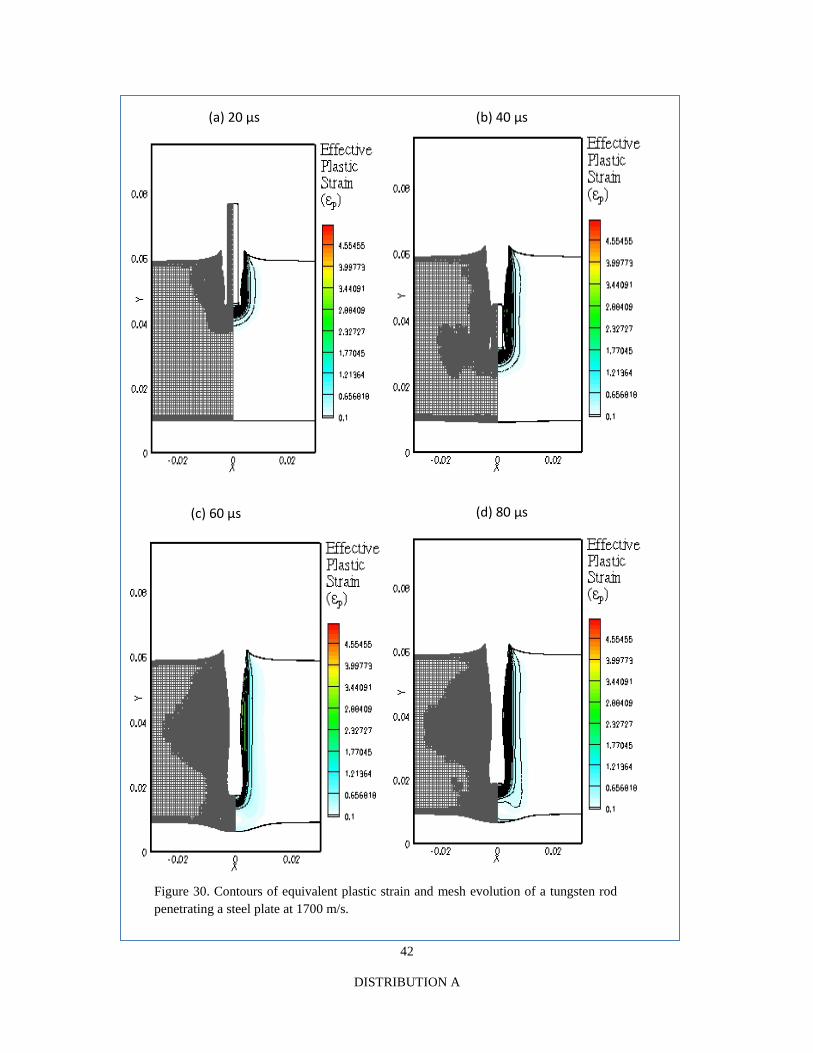
42

DISTRIBUTION A

(a) 20 µs (b) 40 µs

(c) 60 µs (d) 80 µs

Figure 30. Contours of equivalent plastic strain and mesh evolution of a tungsten rod penetrating a steel plate at 1700 m/s.

43

DISTRIBUTION A

(a) 20 µs (b) 40 µs

(c) 60 µs (d) 80 µs

Figure 31. Snapshots of the interface topology of a tungsten rod penetrating a steel plate at 1700 m/s.

44

DISTRIBUTION A

Figures 28 (a) & 28 (b) show the projectile nose and tail trajectories and velocities as a function of time, which are compared with the superposed results from experiment and numerical calculations [10, 13]. Also plotted are the initial positions of the rear and impact surface. The predicted penetration depths are in good agreement with experiments. The present work appears to produce better agreement with experiments when compared to previous calculations [10, 13].

The next set of calculations correspond to the impact velocity of 1700 m/s. The results from the current caclulations are presented in Figures 30, 31 & 32. The contours of effective plastic strain ( )Pε and

Figure 32. Projectile nose and tail (a) trajectories and (b) velocities of a tungsten rod penetrating steel plate at 1700 m/s.

45

DISTRIBUTION A

velocity, the evolution of mesh and the interface topology, for the impact velocity of 1700 m/s, are plotted in Figures 29, 30 & 31. The maximum equivalent plastic strain recorded for this impact velocity is around 5.0. The maximum value and the distribution of the plastic strain reported in [2] agrees very well with the present computations. In contrast to the lower impact velocity (1250 m/s), the projectile is completely consumed by the target forming a slightly larger crater and longer penetration depth. Similar to the lower impact velocity case, the rod comes to rest with only small residual velocities around 80µs. To validate the computations, the trajectories and the velocity histories for the nose and tail of the projectile are plotted in Figure 32. Also shown in the figure are the superposed results from experimental observations and numerical calculations [2]. As evident from the figure, the numerical results are in excellent agreement with experiments. The example clearly validates the current method for very different speeds of interactions.

8.1.3 SHOCK WAVE INTERACTION WITH HEMISPHERICAL GROOVE

In this example, a planar shock wave interacting with a hemispherical groove in a Copper matrix is considered. This model can also be viewed as a prototype for a hemispherical Explosively Formed Projectile (EFP). A planar shock wave generated by contact explosion interacts with a hemispherical groove of radius 15 mm (Figure 33). The generated shock wave corresponds to a particle velocity of 540 m/s and a pressure ratio of 230 Kbar . The center of the groove is located at 29 mm from the bottom surface of the plate. The shock is initiated by accelerating the velocity at the bottom domain from 0 to 540 m/s. A computational domain of 250 mm × 30 mm is chosen. A base mesh of size gx 0.003∆ = with 4 levels of

mesh refinement is selected. The simulation is run to T = 100 µs. The Johnson-Cook material model is employed to simulate the response of the Copper matrix.

46

DISTRIBUTION A

Figure 33. Snapshots of velocity contours and mesh evolution at different instants in time for the response of a hemispherical groove to a shock wave.

47

DISTRIBUTION A

The interaction of the shock wave with the hemispherical groove results in a reflected expansion wave and formation of a jet as documented in the experimental work reported in and subsequently in the numerical work reported in . The jet reaches a maximum velocity of 2750 m/s at about 12 µs and continues to jet until it reaches the target. The maximum jet velocity and the jet diameter obtained from the present calculations are compared with the previous computational and experimental observation in Table 4. The mesh topology and the velocity contours are shown in Figure 33. In Figure 34, the interface topology at different instants in time are plotted. The evolution of the interface closely follows the results reported in .

Table 4: Comparison with experimental and computational results for the jet velocity and diameter.

Velocity (cm/s) Diameter ( cδ , cm)

Present 0.275 0.58

Computation 0.264 0.62

Experiment 0.27 0.6

Figure 34. Topology and evolution of the interface at different instants in time for the response of a hemispherical groove to a shock wave.

48

DISTRIBUTION A

8.1.4 PERFORATION OF ALUMINUM PLATES BY CONICAL-NOSED PROJECTILE

Numerical simulations of a conical-nosed projectile perforating cylindrical target plates are performed next. The conical nosed projectile is made of Tungsten and the cylindrical target plate is made of 5083-H131 Aluminum. The geometry and the problem set up can be found in the experimental studies conducted in . Prior numerical calculations for this problem have been reported in [2]. Two plates of thickness 12.7 mm and 50.8 mm impacted at velocities 1195 m/s and 1176 m/s respectively are considered. The initial problem configuration is displayed in Figure 35.

The Johnson-Cook material model is employed to simulate the response of the projectile and the target. Consistent with the parameters selected in [2], the Taylor-Quinney coefficient 𝛽 is set to zero. Both the simulations are carried out on a base mesh of size gx 0.001∆ = with four levels of mesh refinement. The

histories of effective plastic strain (𝜀𝑃) along with the mesh evolution are displayed in Figures 36 & 37. The conical nosed projectile, upon impacting the target, forms a hole with cavity diameter equal to the shank diameter of the projectile. As reported in [13, 92] , the impacting projectile is practically undeformed for both incident velocities. This can be readily seen from the snapshots displayed in the Figures 36 & 37. The sharp conical nose of the projectile is retained intact even when the interface is moved using the traditional level set advection procedure (with no Lagrangian particles for correction). The mesh adaptation and evolution displayed in the figures clearly show that the regions with fine mesh are concentrated in regions with significant plastic strain. The maximum effective plastic strain computed for the 12.7 mm thick Aluminum plate is 1.52 which is close to the value (1.50) reported in . However, the value registered for the

Figure 35. Initial configuration for the penetration of Steel target by Tungsten rod.

49

DISTRIBUTION A

50.8 mm thick Aluminum plate is 2.05 which is slightly greater than the value reported in. Nevertheless, the response of the plate closely follows the trends reported in [13, 92].

Figure 36. Snapshots of effective plastic strain (𝜀𝑃) contours and mesh evolution at different instants in time for the perforation of 12.7 mm thick Aluminum plate at an incident velocity of 1195 m/s

50

DISTRIBUTION A

8.1.5 AXISYMMETRIC DYNAMIC-TENSILE LARGE-STRAIN IMPACT-EXTRUSION OF COPPER

An experimental study on the influence of grain size on the response of Copper was conducted in . In this section, the numerical computations of the dynamic extrusion of Copper sphere are presented. The example problem considered here consists of a Copper sphere of 7.6 mm in diameter undergoing a tensile extrusion process. The extrusion process is carried out by impacting the Copper sphere at 400 m/s towards the extrusion die. The extrusion die made of hardened Steel is designed with an entrance diameter of 7.62 mm and an exit diameter of 2.28 mm, a reduction of 70 % in cross sectional area as shown in the Figure 38. A base mesh of size gx 0.0005∆ = is chosen with 4 levels of mesh adaptation. The Johnson-Cook

material model is employed to capture the response of the sphere and the extrusion die.

Figure 37. Snapshots of effective plastic strain (𝜀𝑃) contours and mesh evolution at different instants in time for the perforation of 50.8 mm thick Aluminum plate at an incident velocity of 1176 m/s

51

DISTRIBUTION A

The evolution of the effective plastic strain ( )Pε and velocity contours at different instants in time are

displayed in Figure 39. The initial impact of the sphere (at about 10µs corresponding to the instant shown in Figure 39) on the extrusion die results in the acceleration of the leading edge of the sphere as it exits the die . At about 20µs, corresponding to the instant shown in Figure 23, the conical-shaped portion of the sphere comes to rest in the extrusion die. This can be easily verified from the velocity contours registered in Figure 39 and in the subsequent Figures 40 & 41. A portion of the sphere continues to remain at rest in the die while the leading edge of the sphere stretches to form a shape-charge jet. Figure 24 shows the onset of the initial necking process which subsequently forms three major fragments (as verified by the experimental observations ). These fragments are clearly visible in the Figure 41. The jet continues to stretch and results in further splitting up of fragments that can only be captured with explicit damage models. Despite the lack of a damage model, the present calculations are able to predict the overall behavior of the extrusion process that matches well with the experimental predictions reported in . The

maximum equivalent plastic strain ( )Pε was observed during the jetting phase and corresponds to a value

of 9.3. The numerical computations conducted in reports a value of 9.0, which is in close agreement with the current predictions.

Figure 38. Initial configuration for the axisymmetric dynamic-tensile impact-extrusion of Copper.

52

DISTRIBUTION A

Figure 39. Snapshots of effective plastic strain and velocity contours at different instants in time for the dynamic tensile extrusion of Copper.

(a) 10 µs (b) 20 µs

(c) 30 µs (d) 40 µs

53

DISTRIBUTION A

Figure 40. Snapshots of velocity contours and mesh evolution at different instants in time for the dynamic tensile extrusion of Copper.

(a) 10 µs (b) 20 µs

(c) 30 µs (d) 40 µs

54

DISTRIBUTION A

8.2 HANDLING OF FRAGMENTS IN CASE OF SEVERE PLASTIC DEFORMATION

Most of the cases shown in section 8.1 deals with plastic deformation of material in the event of high speed impact or penetration. Generally in case of high speed impact or penetration of a hard impactor on soft target, the target undergoes negligible elastic deformation and then severe plastic deformation. Finally if the speed of impactor is very high and the target is not thick enough to completely absorb the energy of incoming impactor, the resultant scenario can lead to total fragmentation of target material. The example consider here consist of a slender tungsten target penetrating a thin aluminium plate at 1250 m/s. The dimensions of impactor and target are shown in Figure 42. A computational domain of radius 15 mm and length 32.0 mm is chosen for this simulation. The top and right end of the computational domain are prescribed with Neumann conditions. The presence of rigid wall on the bottom end of the domain is modeled by enforcing a reflective condition. The left end of the domain is prescribed with symmetry condition (with Sxy = 0).

The simulation was done using three different mesh sizes of 0.0001 m, 0.00005m and 0.000025m respectively to see the grid dependence as shown in Figure 43 . It was observed that grid size smaller than 0.00005 doesnot change solution to much extent. The snapshot of target and impactor for three different mesh sizes at 12µs.

Figure 41. Topology and evolution of the interface at different instants in time for the dynamic tensile extrusion of Copper

55

DISTRIBUTION A

The results for total framentation is shown in Figure 44. The tungsten rod completely penetrators the steel target resulting in small fragments. The projectile and the part of target then interacts with the rigid surface resulting in high speed impact and total deformation of both projectile and target. Finally the tiny fragments separated from steel target interacts with deformed tungsten projectile shown in Figure 44.

The results shown here are totally besed on resolution and not on a damage model. The idea here is to extend the methodology by using a damage model where the parts of material will be physically separated due to the state of stress.

0.0025m

Tungsten

0.015m

0.005m

V=-1250 m / s

Steel

0.03 m

Figure 42. Initial configuration for the penetration and fragmentation of Steel target by Tungsten rod

56

DISTRIBUTION A

Figure 43. Snapshot of tungsten rod penetrating into a steel target at 12µs for different mesh sizes (a) 0.0001 (b) 0.00005 (c) 0.000025

(b)

(c)

(a)

57

DISTRIBUTION A

Figure 44. Total fragmentation of steel target as different times,(a)-(h),5µs - 40µs

(b) 10µs

(g) 35µs (h) 40µs

(f) 30µs (e) 25µs

(d) 20µs (c) 15µs

(a) 5µs

58

DISTRIBUTION A

8.3 VALIDATION OF PARALLEL ALGORITHM

In this section, validation of the parallel solution of moving boundary problems will be presented. A standard solid impact test case is solved to demonstrate the successful treatment of the GFM approach with an embedded boundary defined by a levelset in parallel setting Thereafter, the main problem of 3-dimensional material dynamics is addressed. This problem typically required large scale computing and thus utilizes the full functionality of the parallelized solver.

8.3.1 AXISYMMETRIC TAYLOR BAR TEST AT 227 M/S

The Taylor test is used as a canonical test problem to verify and validate numerical and experimental observations. This is a two dimensional case in which a cylindrical rod made of copper impacts a rigid flat substrate at 227m/s. A computation domain of radius 15.0mm and length of 34.0 mm is chosen for this simulation. The top and right ends of domain are prescribed with Neumann boundary conditions. The presence of rigid wall at the bottom end of domain is modeled by enforcing a reflective boundary condition. The left end of domain is prescribed with symmetry condition. The simulation used 4 processors with a mesh size of 0.075 mm. The rod has an initial density of 8930 kg/m3, Young’s Modulus of 117GPa, Poisson’s ratio of 0.35, and yield stress of 400MPa. The material is assumed to harden linearly with plastic modulus of 100MPa. The calculations are carried up to 80µs at which point nearly all the initial kinetic energy has been

dissipated as plastic work. Figure 45 shows the contours of pressure and effective plastic strain at the final time of 80µs. Table.5 shows the comparison of present results on the Taylor bar impact case with other computer codes.

Table 5. Comparison of results for axisymmetric impact of copper bar 1t 227 m/s.

Case 227 m/s Final length (mm) Final Base Radius (mm) Maximum EPSBAR

Current setting 21.45 6.8 3.0

Camacho et al[2] 21.42-21.44 7.21-7.24 2.97-3.25

Tran et al 21.15 7.1 2.86

8.4 THREE DIMENSIONAL RESULTS

FIGURE 45. Snapshots of pressure and effective plastic strain at 80 µs

59

DISTRIBUTION A

The results shown in this work are three-dimensional impact of Taylor bar , perforation and ricochet phenomenon in thin plates and total fragmentation of a thin plate. These results are obtained by solving the hyperbolic system of equations, Eq(1-4) using a third-order TVD-based Runge-Kutta scheme for temporal discritization and a third-order convex scheme for spatial discretization. These numerical schemes are well established and details for these can be seen in above-mentioned references. The parameters corresponding to Mie-Gruneisen E.o.S and Johnson-Cook material model are given in Table

8.4.1 TAYLOR BAR IMPACT

In this section we will show two cases of impact of a copper rod on a rigid surface. The first case is a benchmark problem, impact at 227 m/s and the second case is impact at 400m/s to show the handling of high deformation and strain rates.

8.4.1.1 IMPACT AT 227 M/S

During World War II, Taylor conducted an analysis on specimens deformed at very high rates of strain . These experiments involved impact of a cylindrical specimen over a rigid flat substrate, depicted the deformation process as a sequence of elastic and plastic wave propagation into the cylinder. The Taylor bar impact test is a standard test problem to verify and validate numerical and experimental observations. A copper bar of length 32.4 mm and 3.2 mm radius impacts on a rigid flat surface at 227 m/s. The computational domain consists of cuboid of dimensions 16 mm X 16 mm X 34 mm. The domain decomposition is shown in Figure 46 below. The bottom surface of the domain is given reflective boundary conditions and all other surfaces are prescribed with Neumann boundary condition. The standard material properties for copper are used which can be found in high speed impact literature [10, 13].

The mesh chosen is uniform with mesh size of 0.15 mm. The numerical simulation is performed to a time of 80 µs which marks the end of deformation process with material being deformed plastically. The results for Y-direction velocity during the course of simulation are shown in Figure 47. These results give good agreement with experimental analysis. The two key things found in experimental analysis was that the deformed part presents a “mushroom” at the end that is accentuated as the velocity of impact increases and the boundary between the plastically deformed and the undeformed regions cannot be easily seen. The “mushroom” part is observed in following simulations with the radius of the mushroom increasing with increase in impact velocity.

Figure 46. Load balanced domain decomposition created using METIS

60

DISTRIBUTION A

As observed by Taylor, the process of deformation is a sequence of elastic and plastic wave propagating to cylindrical bar. Initially the elastic wave is faster than the plastic wave and travels until it reaches the back surface of Taylor bar. It then reflects towards the plastic wave as a relief wave marking the end of deformation process. It was noticed that the jetting phenomenon continued till 40 µs at which point material begins to harden resulting in bulging at the base of material. The other observable quantities such as pressure and effective plastic strain at the cross section of bar is shown in Figure48 and Figure49.It was also observed that the effective plastic strain is concentrated mostly at the base of bar, Figure49.

Figure 47. Y-direction velocity contours at a cross-section of Taylor bar at 20µs, 40µs, 60 µs and 80µs in clockwise direction starting from top left.

61

DISTRIBUTION A

Figure 48. Pressure contours at a cross-section of Taylor bar at 20µs, 40µs,

62

DISTRIBUTION A

It is a scalar parameter which grows whenever a material is actively yielding i.e. whenever the state of stress is on the yield surface. The advantage of using level set method which accurately defines the interface and can handle large deformation problems can be seen in Figure 50 by mesh containing Taylor bar at the beginning and at the end of simulation. This also depicts the advantage of localization of information on each processor as explained in section 6.

Figure 49. Effective Plastic Strain contours at a cross-section of Taylor bar

63

DISTRIBUTION A

Finally the impact time history of the variation of the dimensions of the bar was compared with LSDYNA 3D code , IPSAP method and parallel 3D PIM code as shown in Table.6. It also depicts that the results are in good agreement with other references.

Table 6 Comparison for three-dimensional Taylor bar Impact problem

Code Final length (mm) Final Radius (mm)

Parallel 3D PIM 21.6 7.1

IPSA 21.52 7.0

LS-DYNA 21.23 6.18

Current work 21.80 6.36

8.4.1.2 IMPACT AT 400 M/S

This section will briefly show the results at higher impact velocity. This impact simulation at 400m/s shows that the current method can handle large deformations and strain rates. The results from this simulation are shown in Figure 51. It can be seen that the deformation is very severe in this case with bar reducing to one third of its initial height.

Figure 50. Mesh defining the topology of Taylor bar at the beginning (left) and at the end (right) of simulation

64

DISTRIBUTION A

The final value of effective plastic strain has also increased to 3.7 as the jetting phenomena lasts longer compared to slower impact at 227m/s.

8.4.2 PERFORATION AND RICOCHET PHENOMENON IN THIN PLATES

Most of the impacts in everyday life occur at an angle and are not inline. The real test of a three dimensional multi-material code is to simulate impact/penetration phenomena at an angle. In this section, three-dimensional high speed impact dynamics of two bodies is shown. A mild steel sphere with velocity of 610 m/s is impacted on a mild steel plate at an angle of 60 degrees. The diameter of mild steel is 6.35 mm and the dimensions of plate are 40 mm X 25 mm X 1.5 mm as show in Figure 52. The material properties and E.o.S. parameters are given in Table 1 and Table A.2.1 respectively.

Figure 51. Y-direction velocity contours and Effective plastic strain for Impact at 400m/s at 80µs.

65

DISTRIBUTION A

A uniform mesh size of 0.1 mm is used with total number of grid points close to 16 million. The simulation is done using 64 processors. The initial mesh topology of sphere and plate is shown in Figure 53.

The high speed sphere undergoes a sphere deformation and ricochets from plate as shown by section view in Figure 54. The velocity vectors shown in Figure 54 illustrate the ricochet phenomena observed during impact at high angles.

Figure 53. Initial mesh topology of mild steel sphere and mild steel plate.

Figure 52. Initial setup of mild sphere impact on a thin mild steel plate.

66

DISTRIBUTION A

The section views of final deformation shown in Figure 55(a) and 55(b) are in excellent agreement with experimental results and Lagrangian numerical computations[27, 30].

The interface topology at different instants of time is shown in Figure 56.

Figure 55. Mild steel impact at 610m/s (a) Side view of deformed sphere (b) Top view of deformed sphere.

Figure 54. Section view of impacted sphere and plate with velocity vectors showing ricochet phenomenon.

67

DISTRIBUTION A

The velocity contours of inclined impact are shown in Figure57 and Figure58. The sphere at high speed comes to rest at 80μs.

Figure 56. Interface topology at 20µs, 40µs, 60 µs and 80µs in clockwise direction starting from top left.

68

DISTRIBUTION A

Figure 57. Y-direction velocity contours of mild steel impact at 20µs (top) and 40μs (bottom).

69

DISTRIBUTION A

8.4.3 FRAGMENTATION OF A THIN PLATE

Generally in case of high speed impact or penetration of a hard impactor on soft target, the target undergoes negligible elastic deformation and then severe plastic deformation. Finally if the speed of impactor is very

Figure 58. Y-direction velocity contours of mild steel impact at 60µs (top) and 80μs (bottom).

70

DISTRIBUTION A

high and the target is not thick enough to completely absorb the energy of incoming impactor, the resultant scenario can lead to total fragmentation of target material. The example consider here consist of a slender

tungsten target penetrating a thin aluminum plate at 2000 m/s. The material properties and E.o.S. parameters are given in Table 1 and Table A.2.1 respectively.

The diameter of impactor is 1.5mm and its length is 3.5mm. The thickness of target is 1 mm. A computational domain of 10mm X 10mm X 10mm is chosen for this simulation. All the faces except the bottom face of domain are prescribed with Neumann boundary conditions. The bottom face acts as a rigid wall resulting in enforcement of reflective boundary condition. The result for total fragmentation is shown in Figure 59 above. The results shown here are totally besed on resolution and not on a damage model. The idea here is to extend the methodology by using a damage model where the parts of material will be physically separated due to the state of stress.

8.5 RESULTS FOR MULTI-SCALE MODELING USING ANN

Figure 59. Interface topology of impactor and target showing total fragmentation.

71

DISTRIBUTION A

8.5.1 VALIDATION OF THE FLOW SOLVER

The computer code employed in the present work has been extensively validated for a range of compressible multimaterial flow problems [3-5]. However, to ensure the reliability of our code for the present calculations, the drag force for a cylinder in shocked flow was computed using the same parameters

as Drikakis et al. [72]. The comparison of the non-dimensional drag force is shown in Figure 60. The transient drag curves produced by Drikakis et al. and by the present calculations show minimal difference in peak magnitude, even though Drikakis et al. employed Navier-Stokes computations for rather modest Reynolds numbers for their calculations. The similarity of the drag behavior for the Euler and Navier-Stokes computations supports the present inviscid computations for the shock-particle interaction, particularly for the high Reynolds numbers that apply to the particles considered by Boiko et al and targeted in the present work.

8.5.2 EXAMPLES OF ANN LEARNING PROCESS

Figure 60.(a) Comparison of drag versus time curve from the present computations with the Navier-Stokes computation of Drikakis et al. The Mach number was 1.3. (b) The flowfield developed in shown in the form of iso-density contours for a time instant when the shock has passed all the way around the cylinder.

(b) (a)

72

DISTRIBUTION A

Learning a drag law

When a planar shock wave hits a stationary spherical particle and passes over it, the drag force on the particle (i.e. force exerted on the particle) changes throughout shock passage. Such drag versus time curves have been obtained by Tanno et al. [77] in experimental (shock tube) setup. Empirical drag laws used in transporting Lagrangian particles in macro-scale simulations do not capture the transient drag experienced by the particle as the shock passes over it. Instead, some averaged measure of steady drag is available that omits the details of the shock passage. With trained ANNs, however, one can retain the information on the drag versus time for a wide range of parameter space. Thus, information obtained from experiments or computations need not be discarded; it can be learned and retained as “knowledge” by the ANN[95]. This does not imply that a large data set is stored. Once the ANN is trained the information on the drag versus time behavior is stored in the weights attached to the individual neurons in the ANN; the individual data sets used for training can then be discarded. Here an ANN is trained to learn the drag versus time behavior for single particles and clusters.

Single Particle

The force on a stationary particle due to shock passage is simulated first. A grid of 500 by 250 nodes was used and was deemed to be adequate based on the validation case above. The initial location for the shock wave was set to be greater than one cylinder radius away from the cylinder. The shock was allowed

to impact the cylinder and continue to travel and the data for horizontal (drag) force was recorded over time. The particle motion was computed from Newton’s law with the force acting on the particle obtained by integrating the pressure over the particle surface. The chosen Mach numbers allow for comparison to conditions used in various experiments[50, 77]. The resulting drag versus time curves at Mach numbers ranging from 1.1 to 1.5 are shown in Figure 61(a). The ANN was trained using this data set. Following training the ANN was tested for a Mach number of 1.3 by predicting the drag versus time behavior and comparing it with a computed drag versus time curve. The drag versus time curve predicted by the neural network as well as the calculated transient drag curve is displayed Figure 61(b). The neural network was capable of matching the computed drag curve and reproduced the negative drag force at later times for the low Mach number cases. However, in this case, the peak value of the drag was underestimated by the neural network. This lack of agreement near the peak is due to the neural network’s sigmoid activation function and the fact that with the data evenly being distributed, a small number of data points exist near the peak. The resulting unbalanced set causes the neural network to spend more time fitting to the rest of the curve

Figure 61. (a) Computed drag versus time curve for shock impingement on a moving particle. The curves for Mach numbers in the range of 1.1 to 1.5 are shown. The data shown comprises the training set. (b) Comparison of the ANN-predicted drag curve for an intermediate Mach number of 1.3 (testing set) with the drag versus time computed by the code.

(a) (b)

73

DISTRIBUTION A

than the peak. The sharper the peak, the less likely the neural network will produce an accurate depiction. Several solutions including the use of radial or wavelet basis function neural networks ,neural network expansion, multi-resolution and segmentation exist but are left for future work.

Multiple Particles

The drag versus time curve for a single particle with only one interacting shock wave is fairly easily predicted by an artificial neural network. In order to obtain a general drag curve with characteristics that could be applied to any particle embedded in a cloud and in a field with multiple shocklets, data was obtained from selected particles in an ensemble of arrangements. The particles in this case number 41 as illustrated in Figure 62. Simulations were performed with randomly seeded clusters of particles and by defining a “representative particle (RP)” embedded in the flow; much as in the case of “representative elementary volumes” (RVEs) employed in volume-averaged formulations of multiphase flows. One way to define such representative particles is to locate them at the center of a cloud of particles; this avoids edge effects and wave reflections from domain boundaries. The representative particles for one

particular case are illustrated by the outline in Figure 63(a). The boundary conditions were set to simulate a shock tube for comparison to the works Boiko et al. [50], Tanno et al. [77] and Sun et al. [70], with the left edge of the domain as an inlet, the right edge an outlet, and both the top and bottom edges as reflective boundaries. A snapshot of the flowfield obtained can be seen in Figure 62(a).

The drag curves for the designated RPs were extracted by the integration of pressure over the level set boundary; these curves are shown in Figure 62(b). The drag curves of the RPs were then averaged resulting in the bold curve in Figure 62(b). This averaged drag versus time curve is considered to correspond to a representative particle and is used to train the ANN for the particular realization depicted in Figure 61(a).

Apart from the Mach number, the other parameters that can affect the behavior of particles in a cloud include the volume fraction of particles, the particle density relative to the fluid, particle shape, collisions between particles and viscous effects as controlled by the Reynolds number. The last three effects are not considered in this work as they are expected to have secondary effects in the initial phase of shock-particle interactions. Of the three parameters considered, namely Mach number (M), particle density ratio (

𝜌𝑝𝜌𝑓

) and

volume fraction 𝜑𝑝, the effects of the 𝜑𝑝 variable are much more easily verified by direct viewing of the

Figure 62. (a) Schlieren image of the flow field and representative particles for a shocked cloud of particles (Φp = 8%, M=2.8). (b) Drag versus time curves for the selected five particles in the array and the averaged drag (bold line).

(a) (b)

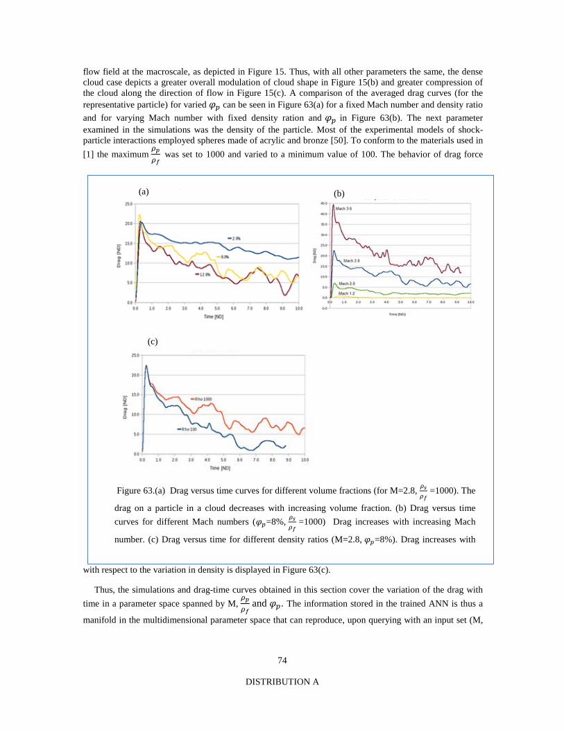
74

DISTRIBUTION A

flow field at the macroscale, as depicted in Figure 15. Thus, with all other parameters the same, the dense cloud case depicts a greater overall modulation of cloud shape in Figure 15(b) and greater compression of the cloud along the direction of flow in Figure 15(c). A comparison of the averaged drag curves (for the representative particle) for varied 𝜑𝑝 can be seen in Figure 63(a) for a fixed Mach number and density ratio and for varying Mach number with fixed density ration and 𝜑𝑝 in Figure 63(b). The next parameter examined in the simulations was the density of the particle. Most of the experimental models of shock-particle interactions employed spheres made of acrylic and bronze [50]. To conform to the materials used in [1] the maximum

𝜌𝑝𝜌𝑓

was set to 1000 and varied to a minimum value of 100. The behavior of drag force

with respect to the variation in density is displayed in Figure 63(c).

Thus, the simulations and drag-time curves obtained in this section cover the variation of the drag with time in a parameter space spanned by M,

𝜌𝑝𝜌𝑓

and 𝜑𝑝. The information stored in the trained ANN is thus a

manifold in the multidimensional parameter space that can reproduce, upon querying with an input set (M,

Figure 63.(a) Drag versus time curves for different volume fractions (for M=2.8, 𝜌𝑠𝜌𝑓

=1000). The

drag on a particle in a cloud decreases with increasing volume fraction. (b) Drag versus time curves for different Mach numbers (𝜑𝑝=8%, 𝜌𝑠

𝜌𝑓 =1000) Drag increases with increasing Mach

number. (c) Drag versus time for different density ratios (M=2.8, 𝜑𝑝=8%). Drag increases with

(a) (b)

(c)

75

DISTRIBUTION A

𝜌𝑝𝜌𝑓

and 𝜑𝑝, 𝑡) the output (drag force). The issue then is how to effectively utilize this stored information in

a macro-scale solver for particle transport.

“Lifting” information from meso-scale calculations

To utilize the correlations obtained above in multi-scale modeling, information must be lifted from the meso-scale. Since the time steps for advancing particles are large compared to the shock passage time over one particle (i.e. each macroscale grid cell containing an ensemble of particles) the drag-time relationship needs to be collapsed into quantities that pertain to macro-scale particle advection time scales. In Lagrangian [ref] and Eulerian [ref] approaches to particle-laden flow computations at the macro-scale, there are two important parameters needed for particle motion. To determine the speed and position of particles the momentum transferred to the particles by the shock is required. Thus, information contained in the drag-time curve can be compressed to extract quantities of interest to the macro-scale particle transport scheme. When viewing a typical shocked particle drag curve (Figure 64), it is evident that there is a maximum value of force that is reached as the shock impinges on the particle and the drag force decays over time. These two characteristic values for a typical drag-time curve are maximum drag coefficient, 𝐶𝑑𝑚𝑎𝑥and relaxation time, τr. Once the drag versus time curve is established and the 𝐶𝑑𝑚𝑎𝑥 and τr is known, the total impulse delivered by the shock, It , can be computed as the area under the curve. For a standard drag curve (obtained from experiment or simulation), we can set τr to be represented by exponential decay and thus the impulse would be:

𝐼𝑡 = ∫ 𝐶𝑑𝑚𝑎𝑥 ∗ 𝑒−𝑡 𝜏𝑟𝑡𝑓

𝑡𝑜 (55)

Figure 64. Illustration of the idea of compressing information contained in the drag versus time for a particular point in parameter space into three pieces of information that are relevant to the macro-scale computations. An exponential fit to the curve is employed to obtain the relaxation time 𝜏𝑟, the maximum drag 𝐶𝑑,𝑚𝑎𝑥 , and the total impulse 𝐼𝑡 delivered by the shock to the particle. The last quantity is computed as the area under the exponential curve fit.

𝐶

𝐼𝑡

𝜏𝑟

76

DISTRIBUTION A

where It is the impulse, to is the impact time, tf is the final time, 𝐶𝑑𝑚𝑎𝑥 is the maximum drag force, t is time, and τr is the relaxation time. In macro-scale calculations, the quantity of interest is It. In addition, since the impulse It acts over a time characterized by τr, once these two values are known, the momentum change of a particle hit by a shock can be calculated. These two pieces of information are all that is needed to quantify a particle’s trajectory in a macro-scale calculation. Thus, the ANN can be trained to learn these two quantities, in place of the drag-time curve, as functions of the parameter set (M,

𝜌𝑝𝜌𝑓

and 𝜑𝑝).

Single particle and particle clusters

For each case presented, the quantified values for particle motion, 𝐶𝑑𝑚𝑎𝑥and 𝜏𝑟 to attain It were found. The value of It and τr were found by numerical integration and fitting an exponential decay function by minimizing the error between the predicted drag curve and the exponential. One such fitting with the impulse highlighted is shown in Figure 64.

Figure 65. (a) ANN convergence behavior for learning the drag law for the multiple particle case. (b) ANN-predicted surface for the maximum drag, (c) ANN-predicted surface for the relaxation time for the particle, (d) ANN-predicted surface for the impulse delivered to the particle.

77

DISTRIBUTION A

The ANN was trained to assimilate the behavior of 𝐶𝑑𝑚𝑎𝑥 , 𝜏𝑟 It for a single particle for the ensemble of cases covering the parameter space. As can be seen from Figure 65, both the It and τr increase with Mach number [75, 77].

With multiple particles the effects of the shock wave interactions in the cluster results in a drag curve that is not monotonic. To ensure that the general behavior of shocked particles is accurately learned by a neural network, data needs to be collected from several representative particles in random placements, i.e. from an ensemble of realizations. The values of 𝐶𝑑𝑚𝑎𝑥 and τr are the two most important parameters that can be directly obtained from the micro-scale calculations. For particle motion that occurs in a dusty gas, the value of 𝜑𝑝 plays a particularly important part; the ANN must learn how the 𝐶𝑑𝑚𝑎𝑥 , τr and It varies with the 𝜑𝑝 in a multiple particle cloud. To assimilate this behavior, 45 different cases were simulated covering

parameter values in the range of 1.2 4.4, 2% 22%, 100 1000sp

f

Mρ

φρ

< < < < < < . Each case had 41

particles placed in a staggered array and then randomly perturbed to simulate a dusty gas. The ANN was trained twice for each input set, with 𝑪𝒅𝒎𝒂𝒙 and τr as outputs. The training period lasted for 5000 iterations with 25 neurons and the convergence curve is seen in Figure 65(a). In Figures 65(b-d) slices through the manifold relating 𝑪𝒅𝒎𝒂𝒙 to combinations of two parameters (while holding the third fixed) amongst M,

𝜌𝑝𝜌𝑓

and 𝜑𝑝 are shown. It is obvious that the major contributor to variations in 𝐶𝑑𝑚𝑎𝑥 is the Mach number. The variation of 𝜑𝑝 has a significant impact on 𝐶𝑑𝑚𝑎𝑥 at higher Mach numbers and the effect of 𝜑𝑝 appears to be non-monotonic at higher Mach numbers. However, from Figure 65 it is observed that in the case of τr, both Mach number and 𝜑𝑝 have significant affects, with increasing influence of the solid fraction at higher Mach numbers.

At this point, it is necessary to assess the level of error associated in the predictions provided by the ANN. While a rigorous error analysis and uncertainty quantification is beyond the scope of this first attempt at effecting multi-scale coupling in the context of shocked flows via an ANN-based modeling technique, the reliability of predictions obtained from the ANN was evaluated. As expected, prediction errors were smaller in the single particle cases because of the rather simpler particle-shock interaction phenomena involved, resulting in a rather smooth drag-time behavior. For the single particle case, testing consisted of randomly selecting a single data point and removing it from the training set. The ANN would be reset and learn the new training set without the removed data point. After training with the remaining data set, the ANN was then queried for the predicted values of 𝑪𝒅𝒎𝒂𝒙 and τr at the test point and was then checked for error (with respect to the DNS output at that point). Testing by selection and removal showed errors all under 2%; therefore for the single particle cases the trained ANN can predict the values of the required outputs to accuracy of a few percent when compared to the full DNS result. For the multiple particle cases, the prediction errors covered a broader range and also depended on the complexity of the manifold being represented. Due to the complex curvature of the manifold (see Figure 65) and some areas of inconsistent trends, the average error for the prediction of randomly removed and tested points inside the ANN prediction curve for It were 7.3%. The largest error for the tested cases resulted from the Mach 4.4 cases which are also responsible for the steep excursions on the plots of 𝐶𝑑𝑚𝑎𝑥 and It. When cases where the Mach number was 4.0 or above was left out and tested for, errors between 12.2% and 14.6% occurred. The errors in prediction of values of 𝐶𝑑𝑚𝑎𝑥 for the multiple particle cases therefore ranged from about 7% in the center of the parameter space to about 12% at the edges of the parameter space. It is likely that further improvements in prediction would result from more advanced ANN training schemes, such as adaptively learning in regions with large functional variations, by changing the architecture of the ANN itself, both in terms of the number of neurons and hidden layers and in terms of the basis function used in the network (for example by using wavelet bases or radial bases instead of the current sigmoid), and by expanding the parameter space and number of samples. All of these issues are being addressed in current work.

78

DISTRIBUTION A

8.5.3 MACRO-SCALE CALCULATIONS

Since the main idea behind using an ANN-based learning scheme is to create an “equation-free” lifting scheme[96, 97], it is necessary to perform macro-scale calculations that employ the information obtained from the ANN to effect Lagrangian particle motion. The resulting particle cloud evolution patterns can then be compared with experimentally observed phenomena, as in Boiko et al to determine if the micro-scale models have provided information that can be useful in making physically correct macroscale predictions. In the above framework, given the Mach number,

𝜌𝑝𝜌𝑓

, and 𝜑𝑝, the ANN can predict 𝐶𝑑𝑚𝑎𝑥 and τr. These

values are then be placed in a Lagrangian algorithm using Newton’s second law and the particle trajectory is calculated.

The trained ANN with the correlation of Mach number, 𝜌𝑝𝜌𝑓

and 𝜑𝑝 to the shock-delivered impulse, It on

a particle, can be used to predict how a shock impacted particle in a cloud will move. The result of using data from the ANN in combination with the Lagrangian particle advection scheme on a single particle inside a cloud can be seen as the solid line alongside the experimental work of Boiko et al. [50] in Figure

Figure 66. Trajectory of an individual particle in a particle cloud. Experimental data from Boiko et al along with their computations based on an empirically fit drag law are shown. The trajectory obtained from the trained ANN for a single particle in a 3% volume fraction cloud is also shown in the figure.

79

DISTRIBUTION A

66. The symbols are directly from experiments, the dashed line is Boiko’s computation, and the solid line is from Lagrangian advection using lifted behavior learned by the ANN. As can be seen the trajectory of a single particle computed from the present scheme is in good agreement with experiments and Boiko et al’s computation using the experimentally derived (fitted) drag law.

Macro-scale simulations were performed by treating the particles as point entities and advecting them according to Newton’s law, with the force acting on the particle drawn by querying the ANN. To ascertain that indeed the formation of the “V” shaped phenomenon is due to that of the variation in 𝜑𝑝 several macro-scale models were performed. They included simulations that were drag law based, with low 𝜑𝑝, with high 𝜑𝑝, and with a uniform band 𝜑𝑝. The initial particle distributions for each of these cases (which correspond to the cases shown in Figure 15(a)-(c)) are displayed in Figure 67 as volume

fraction contours in the macroscopic computational domain. For the sparse dust cloud case (as in Figure 67(a) and 15(a)), Figure 68 shows the evolution of the particle cloud after shock impingement. In this case, particle dispersion occurred without a distinct pattern developing, due to a small variance in𝜑𝑝. This was demonstrated experimentally in Figure 15(a) drawn from Boiko’s experiments. With 𝜑𝑝 and other parameters all the same, each particle should experience the same motion. When the density of particle is increased such as in Figure 15(b), a “V” phenomenon appears (as shown in Figure 69) as seen by Boiko et al. [1]. This phenomenon occurs only at the macro-scale when there is a wide range in 𝜑𝑝. In this case the

Figure 67. Volume fraction fields for the three cases of particle cloud evolution presented. (a) For a sparse cloud of particles (200 particles); (b) For a dense cloud of particles (1000 particles); (c) For a dense column of particles. These three arrangements correspond to those employed in the experiments of Boiko et al.

(a) (b)

(c)

80

DISTRIBUTION A

particles in the center of the cloud lie in a region of higher volume fraction. The particles on the periphery are in a region of smaller volume fraction. The peripheral particles are blown away at a faster velocity by the shock, while those in the center are shielded by other particles and hence move more slowly. It is this shielding effect that leads to the formation the triangular distribution in this case. Thus, the ANN-based meso-scale model that is employed in the macro-scale simulations displays behavior that is observed in experiments.

81

DISTRIBUTION A

Figure 68. Macro-scopic behavior of the particle cloud with particles subject to drag laws derived from the ANN-predicted surface. This case of low volume fraction of the particles retains an amorphous particle cloud in agreement with Boiko et al.’s experiments [2].

(a) Time=0.0 (b) Time = 200.0

(d) Time = 600.0 (c) Time = 400.0

(e) Time = 800.0 (e) Time = 1000.0

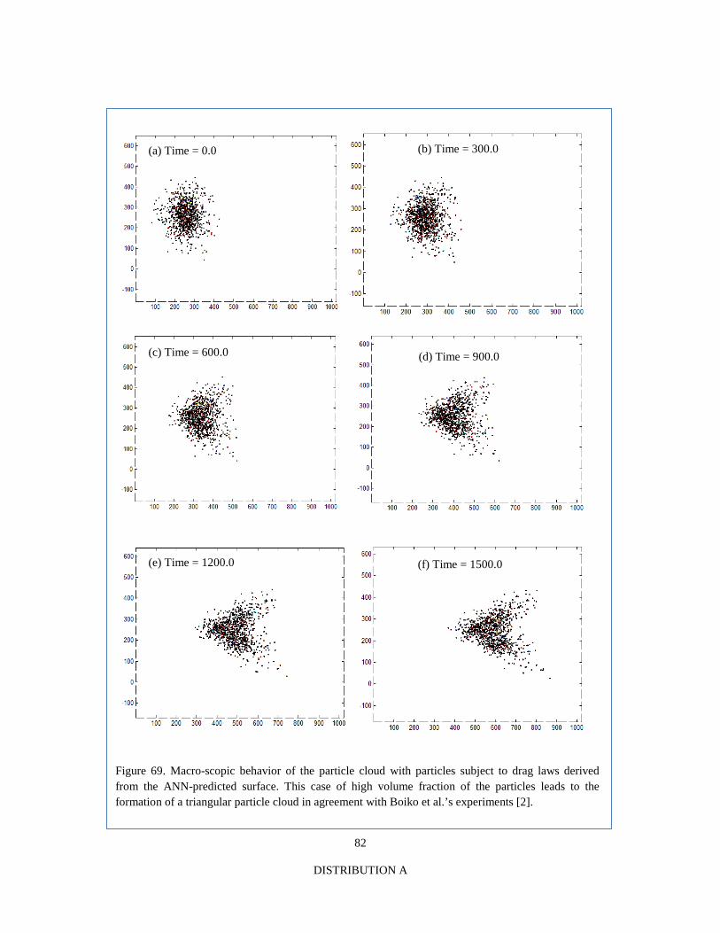
82

DISTRIBUTION A

(a) Time = 0.0 (b) Time = 300.0

(d) Time = 900.0 (c) Time = 600.0

(f) Time = 1500.0 (e) Time = 1200.0

Figure 69. Macro-scopic behavior of the particle cloud with particles subject to drag laws derived from the ANN-predicted surface. This case of high volume fraction of the particles leads to the formation of a triangular particle cloud in agreement with Boiko et al.’s experiments [2].

83

DISTRIBUTION A

(a) Time = 0.0 (b) Time = 300.0

(d) Time = 900.0 (c) Time = 600.0

(f) Time = 1500.0 (e) Time = 1200.0

Figure 70. Macro-scopic behavior of a column of particles with particles subject to drag laws derived from the ANN-predicted surface. This case of high volume fraction of the particles leads to the clustering of the particles in the fore part of the cloud and dispersal in the rear part as seen in experiments[2].

84

DISTRIBUTION A

9 CONCLUSIONS

A sharp interface Cartesian grid-based hydrocode is developed to solve high speed impact, collision, penetration and void collapse problems. The novelty of the approach lies in the manner in which the ghost states are defined. Collisions between interfaces are resolved by employing a simple collision detection algorithm. The proposed hydrocode has been applied to simulate several numerical examples spanning various cases of impact, penetration, ejection and collapse. The robustness, versatility and accuracy of the hydrocode has been established by presenting a variety of benchmarking examples. The results obtained show excellent agreement with experiments and other numerical simulation techniques. In addition, the results obtained from the present approach are shown to be superior to the previous work. The three dimensional extension of method has involved challenging tasks such as implementation of Ghost Fluid method in three dimensions, handling of levelset in parallel setting, localization of data with efficient storage and retrieval and efficient construction of ghost layer for inter processor communication. The proposed method shows good agreement with other numerical techniques. In addition, the three-dimensional results shown in this work are first of a kind in eulerian framework.

10 ACKNOWLEDGEMENTS

The work was performed under the grants from the AFOSR computational mathematics group (Program Manager: Dr. Fariba Fahroo) and from the AFRL-MNAC (Eglin AFB, Program Manager: Dr. Michael E. Nixon)

APPENDIX

A.1 GOVERNING EQUATIONS

Because of high speeds involved in the interaction process, the governing equations comprise a set of hyperbolic conservation laws cast in cartesian coordinates; the governing equations take the following form:

U F G H St x y z

∂ ∂ ∂ ∂∂ ∂ ∂ ∂

+ + + =

[A.1]

For the elastic predictor step, in addition to mass, momentum and energy equations, the constitutive models for deviatoric stress terms are evolved. Thus the conservative variable and the fluxes in EqA.1 take the form given below:

( )( )( )

2

2

2

, , , , , , , , , ,

, , , , ( ), , , , , ,

, , , , ( ), , , , , ,

, , , , ( ),

xx xy yy xz yz zz

xx xy yy xz yz zz

xx xy yy xz yz zz

U u v w E S S S S S S

F u u p uv uw u E p uS uS uS uS uS uS

G v uv v p vw v E p vS vS vS vS vS vS

H w uw vw w p w E p

ρ ρ ρ ρ ρ ρ ρ ρ ρ ρ ρ

ρ ρ ρ ρ ρ ρ ρ ρ ρ ρ ρ

ρ ρ ρ ρ ρ ρ ρ ρ ρ ρ ρ

ρ ρ ρ ρ ρ

=

= + +

= + +

= + +

( ), , , , ,xx xy yy xz yz zzwS wS wS wS wS wSρ ρ ρ ρ ρ ρ

[A.2]

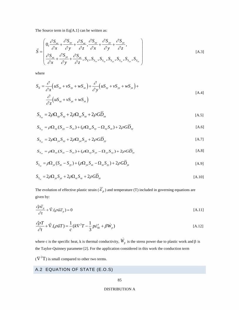
85

DISTRIBUTION A

The Source term in Eq[A.1] can be written as:

0, , ,

, , , , , , ,xx xy yy xz yz zz

xy xy yy yzxx xz

yzxz zzE S S S S S S

S S S SS Sx y z x y z

SSS S S S S S S S S

x y z

∂ ∂ ∂ ∂∂ ∂∂ ∂ ∂ ∂ ∂ ∂

∂∂ ∂∂ ∂ ∂

+ + + +

=

+ +

[A.3]

where

( ) ( )

( )

E xx xy xz xy yy yz

xz yz zz

S uS vS wS uS vS wSx y

uS vS wSz

∂ ∂∂ ∂∂∂

= + + + + + +

+ + [A.4]

2 2 2xxS xy xy xz xz xxS S S GDρ ρ ρ= Ω + Ω + [A.5]

( ) ( ) 2xyS xy yy xx xz zy zy xz xyS S S S S GDρ ρ ρ= Ω − + Ω − Ω + [A.6]

2 2 2yyS yx xy yz yz yyS S S GDρ ρ ρ= Ω + Ω + [A.7]

( ) ( ) 2

xzS xz zz xx xy yz yz xy zzS S S S S GDρ ρ ρ= Ω − + Ω − Ω + [A.8]

( ) ( ) 2yzS yz zz yy yx xz xz xy yzS S S S S GDρ ρ ρ= Ω − + Ω − Ω + [A.9]

2 2 2zzS yz yz xz xz zzS S S GDρ ρ ρ= Ω + Ω + [A.10]

The evolution of effective plastic strain ( pε ) and temperature (T) included in governing equations are

given by:

.( ) 0ppu

t∂ρε

ρ ε∂

+ ∇ = [A.11]

21 1.( ) ( )3

ekk p

T uT k T p Wt c

∂ρ ρ ε β∂

+ ∇ = ∇ − + [A.12]

where c is the specific heat, k is thermal conductivity, pW is the stress power due to plastic work and β is

the Taylor-Quinney parameter [2]. For the application considered in this work the conduction term

(

∇2T) is small compared to other two terms.

A.2 EQUATION OF STATE (E.O.S)

86

DISTRIBUTION A

Closure for the set of governing equations is obtained by modeling the dilatational (pressure) response of the material using a suitable equation of state. To this effect, the pressure, specific internal

energy and specific volume 1(V )ρ= are coupled through a relation of the form:

cc

( e e (V )) eP( e,V ) (V ) P (V ) f (V )V V

−≈ + = +Γ Γ

[A.13]

where ec and Pc denote the reference internal energy and pressure at 0 K. The E.O.S shown in Eq[A.13] is the incomplete Mie-Grüneisen formulation . Eq[A.13] can also be viewed as the first-order approximation of the state surface in the neighborhood of the measured Hugoniot curve along an isochoric path . (V )Γ in Eq [A.13] is the Grüneisen parameter defined as

0 0v

P(V ) V |e

∂ = = ∂

Γ ρΓ

ρ [A.14]

where 𝜌0 is the density of the unstressed material. As pointed out in , it is important to note that the Mie-Grüneisen formulation is not applicable for problems with phase change.

Material 0

3( Kg / m )ρ

ν c

(W / m K )− K( J / Kg K )− 0Γ 0c

( m / s ) S

Copper 8930 0.35 383.5 401 2.0 3940 1.49

Tungsten heavy alloy

17600 0.29 477 38 1.43 4030 1.24

High-hard steel

7850 0.30 134 75 1.16 4570 1.49

Aluminum 2700 0.30 896 166.9 1.99 5386 1.339

Mild Steel 7870 0.3 481 38.0 2.17 4569 1.49

Table A.2.1: Parameters for the Mie-Grüneisen E.O.S. for commonly used materials

Accommodating for negative pressure (tension) and preserving the positivity of sound speed-squared, the function f(V) in Eq[A.13] is written as

87

DISTRIBUTION A

20 0

0 02 2

20 0

0

1 ( )2(1 )

( )1 1

cV V V V

Vsf V

c V VV V

Φ Γ − − ∀ ≤ − Φ = − ∀ >

ρ

[A.15]

In the above expression, the constants c0 is the bulk sound speed and 𝑠 is related to the isentropic pressure derivative of the isentropic bulk modulus . The c0 and s are coefficients relate the shock speed Us and the particle velocity UP. Experiments on solids provide a relation between Us and Up. A first approximation consists of a linear relation given as

[A.16]

The expression for the speed of sound in the material is then given by

22

e

P P P Pc e f '(V )ρ

∂ ∂= + = Γ + + Γ ∂ρ ∂ρ ρρ

[A.17]

The parameters for the Mie-Grüneisen E.O.S. for some of the materials used in this work are given in Table A.2.1.

A.3 CONSTITUTIVE RELATIONS

The response of materials to high intensity (shock/impact) loading conditions are modeled by assuming the additive decomposition of strain,

E P

ij ij ijD D D= + [A.18]

where 𝐷𝑖𝑗 is the total strain-rate tensor given as,

12

jiij

j i

uuD

x x

= +

∂∂∂ ∂

[A.19]

EijD and P

ijD are the elastic and plastic strain-rate components respectively, and ui is the velocity

component. The validity of additive strain rule can be justified for the relatively small elastic strain-rate experienced in the high speeds considered in this work. Assuming incompressibility of the plastic flow

Pij( tr( D ) 0 )= , the volumetric or dilatational response is governed by an equation of state while the

deviatoric response obeys a conventional flow theory of plasticity [10, 99]. Hence, the total stress in the material can be expressed as

ij ij ijS P= −σ δ [A.20]

s 0 pU c sU= +

88

DISTRIBUTION A

where ijσ is the Cauchy stress tensor, Sij is the deviatoric component and P is the hydrostatic pressure

taken to be positive in compression. Using Eq[A.18], the rate of change of deviatoric stress component can be modeled using the hypo-elastic stress-strain relation:

ˆ 2 ( )Pij ij ijS G D D= − [A.21]

where ijS is the Jaumann derivative .

ˆij ij ik kj ik kjS S S S= + Ω − Ω [A.22]

and ijΩ is the spin tensor. The Jaumann derivative is used to ensure objectivity of the stress tensor with

respect to rotation. The spin tensor used in Eq[A.22] is given by:

12

jiij

j i

uux x

∂∂∂ ∂

Ω = −

[A.23]

The deviatoric strain-rate component, ijD , in Eq[A.21] is given by:

13ij ij kk ijD D D δ= −

[A.24]

The isochoric plastic strain-rate component P Pij ij( D D )= in Eq[A.18] is modeled assuming a coaxial flow

theory (Druckers' postulate) for strain hardening materials :

pij ijD N= Λ [A.25]

where ijij

kl kl

SNS S

= is the unit outward normal to the yield surface and Λ is a proportional

positive scalar factor called the consistency parameter . The consistency parameter Λ is determined using J2

Von Mises yield condition. The effective plastic stress (Se) and the effective plastic strain-rate p( )ε are

given by:

2 3 ( : )2e ij ijS S S=

[A.26]

2 22 2( ) ( : )3 3

P PP ij ijD Dε = = Λ

[A.27]

The evolution of temperature due to heat conduction and thermal energy produced by work done during elasto-plastic deformation is written as

89

DISTRIBUTION A

2

3ekk p

pCT k T Wρ ε β= ∇ − + [A.28]

where T is the temperature, C the specific heat, 𝑘 thermal conductivity, 𝑝 is the stress power due to plastic work and 𝛽 is the Taylor-Quinney parameter . The Taylor-Quinney parameter implies the fraction of mechanical power converted to thermal power and is taken as 0.9. The stress power due to plastic work is given by

P P eW S= ε

[A.29]

where Se is the Von-Mises effective stress Eq[A.26]. For the applications considered in this work, the conduction and elastic work terms are small in comparison with the plastic stress power term 𝑝.

A.4 RADIAL RETURN MAPPING ALGORITHM

The plastic deformation of material is governed by the yield function that constrains the stress to remain on or within the elastic domain:

( , ) 0ijf S ξ ≤ => admissible stress state [A.30]

( , ) 0ijf S ξ > => inadmissible stress state [A.31]

where f is a generic yield function and ξ is a scalar or tensor hardening parameter.

In an operator splitting algorithm for elasto-plastic material, if the predicted “trial” elastic state (determined by freezing the plastic flow) falls within the yield surface, i.e. 0f < , then the deformation is purely elastic and the final stress state is indeed the predicted trial state. The yield and subsequent plastic flow is said to have occurred when 0f = . The inadmissible trial state for 0f > is corrected by bringing the stress back to

the yield surface by enforcing the consistency condition 0f = , along a direction normal to the yield

surface (ij

fσ

∂∂

).In this work , the algorithm adopted is explained below.

The radial return algorithm due to Ponthot et al is based on J2 Von-Mises flow theory which assumes the existence of yield function (for isotropic materials) of the form

( , ) 0ij Y e Yf S Sσ σ= − = [A.32]

with hardening law given by

23Y hσ = Λ [A.33]

90

DISTRIBUTION A

Where Yσ is the current yield stress which can be determined using material models and h (also called

plastic modulus) is the slope of effective stress versus effective plastic strain curve under uniaxial loading. Using Eq [A.27] , the yield stress can be written as

PY ijhσ ε= [A.34]

When elastic deformation occurs, 0f < and 0Λ = . Plastic deformation is said to occur when consistency

condition holds true, ( , ) 0ij Yf S σ = . Thus, for elastic and plastic deformation, f and Λ can be obtained

from the Kuhn-Tucker conditions of optimization theory

0, 0, 0f fΛ = Λ ≥ ≤ [A.35]

Possible cases of loading and unloading behavior are:

i. If the stress state is inside the yield surface

0 0f < => Λ =

ii. If the stress state is on the yield surface ( 0f = ), plastic consistency condition should be checked,

which states that 0fΛ = , 0Λ > => 0f =

a) Elastic unloading => 0f < => 0Λ =

b) Neutral loading => 0f = => 0Λ =

c) Plastic loading => 0f > => Violation of 0f ≤

Hence 0Λ > .

In conjunction with operator splitting algorithm, deviatoric stress update

2 ( )Pij ik kj ik kj ij ijS S S G D D+ Ω − Ω = − [A.36]

is split into two parts- “trial” and “corrector” step. The “trial” elastic state is obtained by freezing the plastic flow ( 0P

ijD = ),

, , , 2ij tr ik tr kj ik kj tr ijS S S GD+ Ω − Ω = [A.37]

where ,ij trS is the trial elastic stress tensor. The plastic corrector step is enforced to bring computed trial

stress back to yield surface:

, 2 2Pij cor ij ijS GD G N= − = − Λ [A.38]

91

DISTRIBUTION A

where ,ij corS is the corrected stress update and ijN is the normal direction in which return mapping is

effected:

,

, ,

ij trij

kl tr kl tr

SN

S S= [A.39]

In discrete form, the plastic corrector step can be written as

, , ,2ij cor ij tr ij trS S GN ζ= − [A.40]

where1

0

t

t

dtζ = Λ∫ , with t0 and t1 denoting the beginning and end of time interval of integration. The

parameter ζ is determined by enforcing the generalized consistency condition, 0f = , at time t=t1.

1, , , ,

3 [( 2 )( 2 )] 02 ij tr ij tr ij tr ij tr Yf S GN S GNζ ζ σ= − − − = [A.41]

Integrating Eqs [A.27] & [A.34] in time, we get

1 023

P Pε ε ζ= + [A.42]

1 0 23Y Y hσ σ ζ= + [A.43]

where “0” and “1” denote the values at t0 and t1, respectively. Substituting for 1Yσ , Eq[A.41]is simplified as

22 2 0, , , ,

4 4 2 2(4 ) (4 ) ( ) 09 3 3 3ij tr ij tr ij tr ij tr YG G S S h S Sζ ζ σ− − + + − = [A.44]

to obtain

0, ,

23

2 (1 )3

ij tr ij tr YS S

hGG

σζ

−=

+ [A.45]

Thus, once ζ is obtained, the correction of the predicted deviatoric stress is performed using Eq[A.40] and the consistency condition is enforced.

92

DISTRIBUTION A

REFERENCES

1. Zukas, J., et al., Impact Dynamics Chapter 5. 1982, John Wiley and Sons, New York.

2. J.Baker, et al., Hypervelocity penetration of plate targets by rod and rod-like projectiles. International Journal of Imapact Engineering., 1987. 5(1-4): p. 101-110.

3. Ahrens, T.J., et al., Impact on the earth, ocean and atmosphere. International Journal of Imapact Engineering., 1987. 5(1-4): p. 13-32.

4. Roddy, D.J., et al., Computer simulations of large asteroid impacts into oceanic and continental sites--preliminary results on atmospheric, cratering and ejecta dynamics. International Journal of Impact Engineering, 1987. 5(1-4): p. 525-541.

5. Benson, D., et al., Particle-level modeling of dynamic consolidation of Ti-SiC powders. Modelling and Simulation in Materials Science and Engineering, 1995. 3: p. 771.

6. Benson, D.J., et al., Dynamic compaction of copper powder: Computation and experiment. Applied physics letters, 1994. 65(4): p. 418-420.

7. Wenzel, A.B., A review of explosive accelerators for hypervelocity impact. International Journal of Impact Engineering, 1987. 5(1-4): p. 681-692.

8. Walters, W.P., et al., Fundamentals of Shaped Charges. 1989: Wiley-Interscience.

9. Udaykumar, H.S., et al., An Eulerian method for computation of multi-material impact with ENO shock-capturing and sharp interfaces. Journal of Computational Physics., 2003. 186(1).

10. Tran, L.B., et al., A particle levelset based sharp interface cartesian grid method for impact, penetration, and void collapse. Journal of Computational Physics., 2004. 193(2): p. 469-510.

11. J.Benson, D., Computational methods in lagrangian and eulerian hydrocodes. Comput. Methods Appl. Mech. Eng., 1995. 99(2-3): p. 235-394.

12. Anderson, C.E., An overview of the theory of hydrocodes. International Journal of Imapact Engineering., 1987. 5(1-4): p. 33-59.

13. Camacho.G.T., et al., Adaptive lagrangian modelling of ballistic penetration of metallic targets. Comput. Methods Appl. Mech. Eng., 1997. 142(3-4): p. 269-301.

14. Zukas, J.A., Introduction to hydrocodes. 2004: Elsevier Science.

15. Xiao, H., et al., Elastoplasticity beyond small deformations. Acta Mechanica, 2006. 182(1): p. 31-111.

16. Naghdi, P., A critical review of the state of finite plasticity. Zeitschrift für Angewandte Mathematik und Physik (ZAMP), 1990. 41(3): p. 315-394.

17. Wu., H.-C., Continuum Mechanics and Plasticity. 2004: Chapman & Hall/CRC Press.

18. Khan, A., et al., Continuum theory of plasticity. 1995: Wiley New York.

93

DISTRIBUTION A

19. Truesdell, C., A first course in rational continuum mechanics. Vol. 1. 1977: Academic Press.

20. Strain, J., Fast tree-based redistancing for level set computations. Journal of Computational Physics, 1999. 152(2): p. 664-686.

21. Strain, J., Tree Methods for Moving Interfaces* 1. Journal of Computational Physics, 1999. 151(2): p. 616-648.

22. Viecelli, J.A., A computing method for incompressible flows bounded by moving walls* 1. Journal of Computational Physics, 1971. 8(1): p. 119-143.

23. Sambasivan, S., et al., Ghost fluid method for Strong Shock Interactions. Part2: Immersed Solid Boundaries. AIAA., 2009. 47(10): p. 2923-2937.

24. Sambasivan, S.K., et al., Sharp interface simulations with Local Mesh Refinement for multi-material dynamics in strongly shocked flows. Computers & Fluids, 2010. 39(9): p. 1456-1479.

25. Sambasivan, S., et al., Ghost Fluid Method for Strong Shock Interactions Part 1: Fluid-Fluid Interfaces. AIAA., 2009. 47(12): p. 2907-2923.

26. R.P.Fedkiw, et al., A non oscillatory Eulerian approach to interfaces in multi-material flows ( the Ghost Fluid Method). Journal of Computational Physics., 1999. 152(2): p. 457-492.

27. Yoo, Y.H., et al., A three-dimensional FE analysis of large deformations for impact loadings using tetrahedral elements. Computational mechanics, 2003. 30(2): p. 96-105.

28. Paik, S., et al., Parallel performance of large scale impact simulations on Linux cluster super computer. Computers & Structures, 2006. 84(10-11): p. 732-741.

29. Hu, W., et al., Parallel point interpolation method for three-dimensional metal forming simulations. Engineering analysis with boundary elements, 2007. 31(4): p. 326-342.

30. Paik, S.H., et al., Parallel performance of large scale impact simulations on Linux cluster super computer. Computers & structures, 2006. 84(10-11): p. 732-741.

31. Cooper, S., et al., A numerical exploration of the role of void geometry on void collapse and hot spot formation in ductile materials. International Journal of Plasticity, 2000. 16(5): p. 525-540.

32. Plohr, B.J., et al., A conservative Eulerian formulation of the equations for elastic flow* 1. Advances in Applied Mathematics, 1988. 9(4): p. 481-499.

33. Plohr, B.J., et al., A conservative formulation for plasticity* 1,* 2. Advances in Applied Mathematics, 1992. 13(4): p. 462-493.

34. Simo, J., et al., General return mapping algorithms for rate-independent plasticity. 1987: Elsevier: Tucson, Arizona.

35. Johnson, G.R., et al., Fracture characteristics of three metals subjected to various strains, strain rates, temperatures and pressures. Engineering Fracture Mechanics, 1985. 21(1): p. 31-48.

36. Sethian., J.A., Levelset Methods and Fast Marching Methods: Evolving Interfaces in computaional geometry, Fluid Mechanics, Computer Vision, and Material Science. 1999: Cambridge University Press.

37. J.A.Sethian., Evolution, implementation, application of levelsets and fast marching methods for advancing fronts. Journal of Computational Physics., 2001. 169(2): p. 503-555.

94

DISTRIBUTION A

38. Aslam, T.D., A partial differential equation approach to multidimensional extrapolation. Journal of Computational Physics, 2004. 193(1): p. 349-355.

39. Dalrymple, R.A., Particle Methods and Waves, with Emphasis on SPH. 2007.

40. Wang, C., et al., An adaptive ghost fluid finite volume method for compressible gas-water simulations. Journal of Computational Physics, 2008. 227(12): p. 6385-6409.

41. Berger, M.J., et al., Local adaptive mesh refinement for shock hydrodynamics. Journal of computational Physics, 1989. 82(1): p. 64-84.

42. Henshaw, W.D., et al., Moving overlapping grids with adaptive mesh refinement for high-speed reactive and non-reactive flow. Journal of Computational Physics, 2006. 216(2): p. 744-779.

43. Udaykumar, H., et al., Adaptively refined, parallelised sharp interface Cartesian grid method for three-dimensional moving boundary problems. International Journal of Computational Fluid Dynamics, 2009. 23(1): p. 1-24.

44. Gropp, W., et al., Using mpi. 1999: MIT press.

45. Karypis, G., et al., Parmetis---parallel graph partitioning and sparse matrix ordering library, version 2.0. Univ. of Minnesota, Minneapolis, MN, 1998.

46. C.W.Shu, et al., Efficient implementation of Essentially Non-Oscillatory shock capturing schemes II. Journal of Computational Physics., 1989. 83(1): p. 32-78.

47. Peigin, S., et al., Parallel large scale high accuracy Navier-Stokes computations on distributed memory clusters. The Journal of Supercomputing, 2004. 27(1): p. 49-68.

48. Cormen, T., Introduction to algorithms. 2001: The MIT press.

49. Carter, J., et al., Universal classes of hash functions. Journal of computer and system sciences, 1979. 18(2): p. 143-154.

50. Boiko, V.M., Kiselev, V.P., Kiselev, S.P., Papyrin, A.N., Poplavsky, S.V., Fomin, V.M., Shockwave Interaction with a Cloud of Particles. ShockWaves, 1997. 7: p. 275-285.

51. Crowe, C.T., Sommerfeld, M. and Tsuji, Y., Multiphase flows with droplets and particles. 1988.

52. Kosinski, P., On Shock Wave Propagation in a Branched Channel with Particles. Shock Waves, 2006. 15(1): p. 13-20.

53. Kosinski, P., Numerical analysis of shock wave interaction with a cloud of particles in a channel with bends. International Journal of Heat and Fluid Flow, 2007. 28(5): p. 1136-1143.

54. Fedorov, A.V., et al., Reflection of a shock wave in a dusty cloud. Combustion Explosion and Shock Waves, 2007. 43(1): p. 104-113.

55. Fausett, L.V., Fundamentals of Neural Networks, ed. D. Fowley. 1994, Upper Saddle River, New Jersey, United States: Prentice-Hall.

56. Nilsson, J., et al., Artificial Neural Networks - A Method for Optimal. Donor-Recipient Matching. Large Scale Simulation of Survival after Heart Transplantation. Journal of Heart and Lung Transplantation, 2010. 29(2): p. S29-S29.

57. Krose, B., et al., An introduction to Neural Networks. 1996, Amsterdam, Amsterdam: The University of Amsterdam.

95

DISTRIBUTION A

58. Unger, J.F., et al., Coupling of scales in a multiscale simulation using neural networks. Computers & Structures, 2008. 86(21-22): p. 1994-2003.

59. Jorg F. Unger, C.K., Coupling of scales in a multiscale simulation using neural networks. Computers & Structures, 2008. 86(21): p. 1994-2003.

60. Ahmadi, M., et al., Estimation of the reservoir permeability by petrophysical information using intelligent systems. Petroleum Science and Technology, 2008. 26(14): p. 1656-1667.

61. Giralt, F., Arenas, A., Ferre-Gine, J., Rallo, R., The simulation and interpretation of free turbulence with a cognitive neural system. Physics of Fluids, 2000. 12(7): p. 1826.

62. Sahimi, M., Fractal-wavelet neural-network approach to characterization and upscaling of fractured reservoirs. Computers & Geosciences, 2000. 26(8): p. 877-905.

63. Unger, J.F., et al., Neural networks as material models within a multiscale approach. Computers & Structures, 2009. 87(19-20): p. 1177-1186.

64. Ghaboussi, J., et al., Autoprogressive training of neural network constitutive models. International Journal for Numerical Methods in Engineering, 1998. 42(1): p. 105-126.

65. Hocevar, M., Sirok, B., Grabec, I., A Turbulent-Wake estimation using radial basis function neural networks. Flow, Turbulence and Combustion, 2005. 74: p. 291-308.

66. Mehratra, K., Mohan, C.K., Ranka, S., Elements of Artificial Neural Networks. 1996, Cambridge: Massachusetts Institute of Technology.

67. Igra, O., Takayama, K., Shock Tube Study for the Drag Coefficient of a Sphere in a Non-Stationary Flow. Proc. R. Soc. Lond., 1993. 442(A): p. 231-247.

68. Rogak, S.N., et al., Stokes Drag on Self-Similar Clusters of Spheres. Journal of Colloid and Interface Science, 1990. 134(1): p. 206-218.

69. Saito, T., et al., The effect of an unsteady drag force on the structure of a non-equilibrium region behind a shock wave in a gas-particle mixture. Shock Waves, 2007. 17(4): p. 255-262.

70. Sun, M., Saito, T., Takayama, K., Tanno, H, Unsteady Drag on a Sphere by Shock Wave Loading. Shock Waves, 2005. 14(1): p. 3-9.

71. Tanno, H., et al., Interaction of a shock with a sphere suspended in a vertical shock tube. Shock Waves, 2003. 13(3): p. 191-200.

72. Drikakis, D., et al., Computation of non-stationary shock-wave/cylinder interaction using adaptive-grid methods. Journal of Fluids and Structures, 1997. 11(6): p. 665-691.

73. Fedorov, A.V., Kharlamova, Y.V., Khmel, T.A., Reflection of a Shock Wave in a Dusty Cloud. Combustion, Explosion, and Shock Waves, 2007. 43(1): p. 104-113.

74. Saito, T., Numerical analysis of dusty-gas flows. Journal of Computational Physics, 2002. 176(1): p. 129-144.

75. Saito, T., Marumoto, M., Takayama, K., Numerical Investigations of Shock Waves in Gas-Particle Mixtures. Shock Waves, 2003. 13: p. 299-322.

76. Saito, T., et al., Experimental and numerical studies of underwater shock wave attenuation. Shock Waves, 2003. 13(2): p. 139-148.

96

DISTRIBUTION A

77. Tanno, H., Itoh, K., Saito, T., Abe, A., Takayama, K., Interaction of a Shock Wave with a Sphere Suspended in a Verticle Tube. Shock Waves, 2003. 13(3): p. 191-200.

78. Sommerfeld, M., The Unsteadiness of Shock-Waves Propagating through Gas-Particle Mixtures. Experiments in Fluids, 1985. 3(4): p. 197-206.

79. Khmel', T.A., et al., Interaction of a shock wave with a cloud of aluminum particles in a channel. Combustion Explosion and Shock Waves, 2002. 38(2): p. 206-214.

80. Igra, O., et al., Shock-Tube Study of the Drag Coefficient of a Sphere in a Nonstationary Flow. Proceedings of the Royal Society of London Series a-Mathematical Physical and Engineering Sciences, 1993. 442(1915): p. 231-247.

81. Ben-Dor, G., et al., Shock wave reflections in dust-gas suspensions. Journal of Fluids Engineering-Transactions of the Asme, 2001. 123(1): p. 145-153.

82. Fedkiw, R.P., Coupling an Eulerian fluid calculation to a Lagrangian solid calculation with the ghost fluid method. Journal of Computational Physics, 2002. 175(1): p. 200-224.

83. Fedkiw, R.P., et al., A non-oscillatory Eulerian approach to interfaces in multimaterial flows (the ghost fluid method). Journal of Computational Physics, 1999. 152(2): p. 457-492.

84. Sambasivan, S., Udaykumar, H.S., An Evaluation of Ghost-Fluid Methods for Strong Shock Interations with Immersed Solid Interfaces. 2009, University of Iowa: Iowa City.

85. Liu, X., et al., Convex ENO high order multi-dimensional schemes without field by field decomposition or staggered grids. Journal of Computational Physics, 1998. 142(2): p. 304-330.

86. Sambasivan, S., et al., Tree-Based Local Mesh Refinement for Compressible Multiphase Flows, in AIAA Proceedings.[np]. 05-08 Jan. 2009, American Institute of Aeronautics and Astronautics, 1801 Alexander Bell Dr., Suite 500 Reston VA 20191-4344 USA,.

87. Taylor., G.I., The use of flat ended projectiles for determining dynamic yield stress. i. theoretical considerations. Proceedings of the Royal Society of London. Series A. Mathematical and Physical Sciences., 1948. 194: p. 289-299.

88. Meyers, M., Dynamic behavior of materials. 1994: Wiley-Interscience.

89. Zhu, Y., et al., Unified and mixed formulation of the 4 node quadrilateral elements by assumed strain method: Application to thermomechanical problems. International journal for numerical methods in engineering, 1995. 38(4): p. 685-716.

90. Anderson, C.E., et al. Penetration of long rods into steel and glass targets: Experiments and computations. in 14th International Symposium on Ballistics, Quebec, Canada. 1993.

91. MALI, V., et al., Study of the disintegration of plane jets(on grooved metal surfaces). Fizika Goreniia i Vzryva, 1974. 10: p. 755-761.

92. Forrestal, M., et al., Perforation of aluminum armor plates with conical-nose projectiles. Mechanics of Materials, 1990. 10(1-2): p. 97-105.

93. Gray III, G., et al. Influence of Shock Prestraining and Grain Size on the Dynamic Tensile Extrusion Response of Copper: Experiments and Simulation. in AIP Conference Proceedings. 2006.

97

DISTRIBUTION A

94. Finnegan, S., et al. A study of obliquity effects on perforation and ricochet processes in thin plates impacted by compact fragments. in Proc. 14th Int. Symp. Ballistics. 1993.

95. Udaykumar, H., et al., An Eulerian method for computation of multimaterial impact with ENO shock-capturing and sharp interfaces. Journal of Computational Physics, 2003. 186(1): p. 136-177.

96. Bishop, C.M., Neural Networks for Pattern Recognition. 1996, USA: Oxford University Press.

97. Chen, L., Debenedetti, P.G., Gear, C.W., Kevrekidis, I.G., From Molecular Dynamics to Coarse Self-Similar Solutions: A Simple Example Using Equation-Free Computation. Journal of Non-Newtonian Fluid Mechanics, 2004. 120(1): p. 215-223.

98. Kevrekidis, I.G., Gear, C.W., Hummer, G., Equation-Free: The Computer-Aided Analysis of Complex Multiscale Systems. Aiche Journal, 2004. 50(7): p. 1346-1355.

99. Hiermaier, S., Structures under crash and impact. Structures Under Crash and Impact, by Stefan Hiermaier. Berlin: Springer, 2008. ISBN 978-0-387-73862-8, 2008. 1.

100. Ponthot., J.-P., Unified stress update algorithms for numerical simulation of large deformation elasto-plastic and elasto-viscoplastic process. International Journal of Plasticity., 2002. 18(1): p. 91-126.

101. J.C.Simo, et al., Computational Inelasticity. 2000: Springer.

DISTRIBUTION LIST

AFRL-RW-EG-TR-2011-167 Defense Technical Information Center 1 Electronic Copy (1 file, 1 format) Attn: Acquisition (OCA) 8725 John J. Kingman Road, Ste 0944 Ft Belvoir, VA 22060-6218 EGLIN AFB OFFICES: AFRL/RWOC (STINFO Tech Library Copy) 1 Copy AFRL/RW CA-N Notice of publication only