A 3D Freehand Ultrasound System for Multi-view Reconstructions from Sparse 2D Scanning Planes

RESEARCH Open Access

A 3D Freehand Ultrasound System for Multi-viewReconstructions from Sparse 2D Scanning PlanesHonggang Yu1, Marios S Pattichis1*, Carla Agurto1, M Beth Goens2

* Correspondence: [email protected] of Electrical andComputer Engineering, Universityof New Mexico, Albuquerque, NM87131, USA

Abstract

Background: A significant limitation of existing 3D ultrasound systems comes fromthe fact that the majority of them work with fixed acquisition geometries. As a result,the users have very limited control over the geometry of the 2D scanning planes.

Methods: We present a low-cost and flexible ultrasound imaging system thatintegrates several image processing components to allow for 3D reconstructionsfrom limited numbers of 2D image planes and multiple acoustic views. Our approachis based on a 3D freehand ultrasound system that allows users to control the 2Dacquisition imaging using conventional 2D probes.For reliable performance, we develop new methods for image segmentation androbust multi-view registration. We first present a new hybrid geometric level-setapproach that provides reliable segmentation performance with relatively simpleinitializations and minimum edge leakage. Optimization of the segmentation modelparameters and its effect on performance is carefully discussed. Second, using thesegmented images, a new coarse to fine automatic multi-view registration method isintroduced. The approach uses a 3D Hotelling transform to initialize an optimizationsearch. Then, the fine scale feature-based registration is performed using a robust,non-linear least squares algorithm. The robustness of the multi-view registrationsystem allows for accurate 3D reconstructions from sparse 2D image planes.

Results: Volume measurements from multi-view 3D reconstructions are found to beconsistently and significantly more accurate than measurements from single viewreconstructions. The volume error of multi-view reconstruction is measured to be lessthan 5% of the true volume. We show that volume reconstruction accuracy is afunction of the total number of 2D image planes and the number of views forcalibrated phantom. In clinical in-vivo cardiac experiments, we show that volumeestimates of the left ventricle from multi-view reconstructions are found to be inbetter agreement with clinical measures than measures from single viewreconstructions.

Conclusions: Multi-view 3D reconstruction from sparse 2D freehand B-mode imagesleads to more accurate volume quantification compared to single view systems. Theflexibility and low-cost of the proposed system allow for fine control of the imageacquisition planes for optimal 3D reconstructions from multiple views.

Yu et al. BioMedical Engineering OnLine 2011, 10:7http://www.biomedical-engineering-online.com/content/10/1/7

© 2011 Yu et al; licensee BioMed Central Ltd. This is an Open Access article distributed under the terms of the Creative CommonsAttribution License (http://creativecommons.org/licenses/by/2.0), which permits unrestricted use, distribution, and reproduction inany medium, provided the original work is properly cited.

mailto:[email protected]

mailto:[email protected]

http://creativecommons.org/licenses/by/2.0

BackgroundThere is a strong interest in developing effective 3D ultrasound imaging systems in

ultrasonography. The basic advantage of 3D systems is that they enable us to provide

quantitative measurements of different organs without assuming simplified geometrical

models associated with conventional 2D systems. Here, our focus is on developing a

3D ultrasound system for accurate 3D reconstructions from arbitrary scanning geome-

tries (freehand) that are validated on calibrated 3D targets.

Most research in 3D echocardiography is focused on the use of 3D probes (volume-

mode probes) where 3D volume is imaged directly from a single probe position. This

approach simplifies the reconstruction and visualization of the 3D data set since the

geometry of acquired slices is known and real-time 3D reconstruction is possible. This

approach does not allow for fine control of the location of the 2D planes.

Clinically, 3D probes have not been widely adopted. The overwhelming majority of

ultrasound exams are still using standard 2D ultrasound probes. Routine clinical diag-

nosis is still depended on acquiring optimal 2D acoustic views. On the other hand, 3D

ultrasound can be used by non-experts to avoid the need for training on how to

acquire optimal 2D views [1]. In current clinical practice, 3D datasets are often com-

municated to expert readers that will then have to extract optimal 2D views that are

needed for documenting clinical diagnosis.

In this paper, we discuss the design of a 3D freehand ultrasound system built from

standard 2D ultrasound machine (see Figures 1, 2). This flexible, very low cost

approach allows for experts control over the acquisition geometry and meets the clini-

cal examination protocol. While the development of 3D freehand ultrasound is cer-

tainly not new [2-7], our focus here is quite different. We are primarily interested in

developing reliable image processing methods that can be used to demonstrate:

• Robust system components:

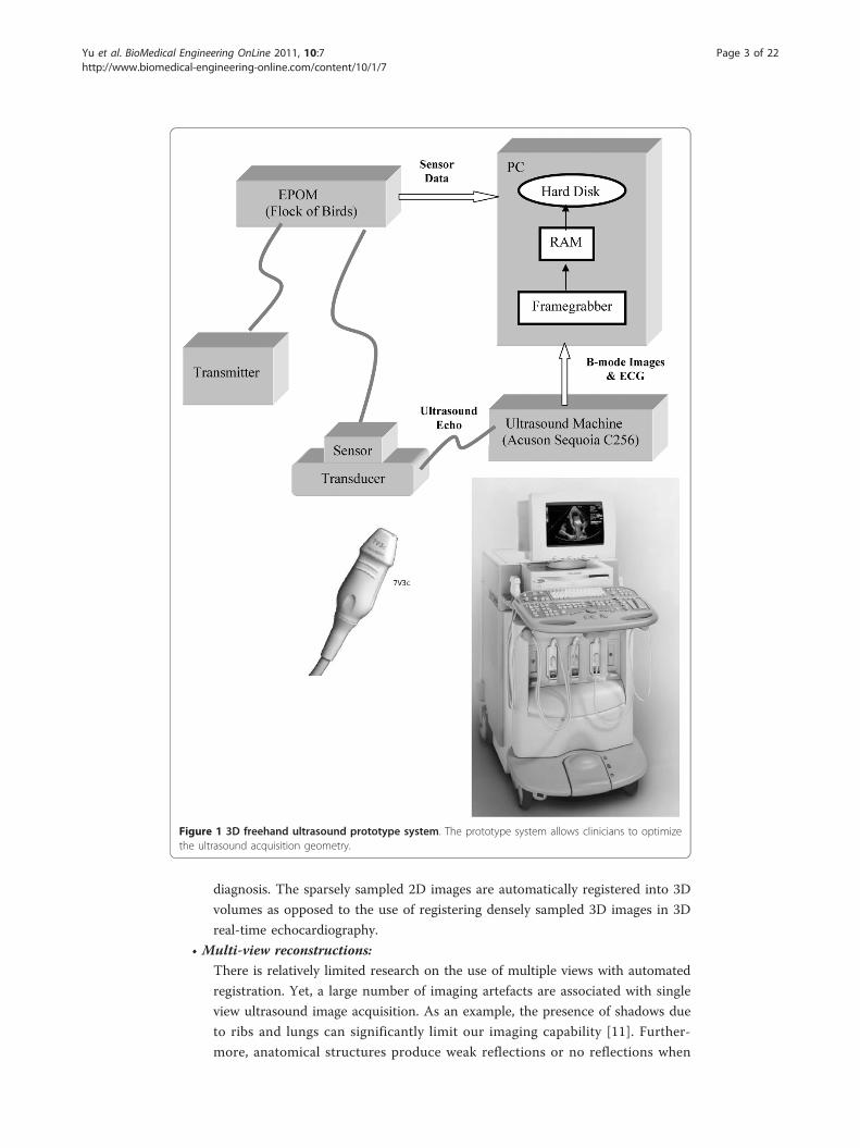
Several required image processing system components (see Figure 2) are often

treated separately in the literature. In this paper, we address several system

issues for reliable performance (see preliminary results in [8-10]). Successful 3D

reconstruction in the system begins with reliable electromagnetic interference

detection for accurate 3D position and orientation sensing. It also requires

accurate 2D to 3D calibration. A hybrid active contour segmentation and para-

meter optimization is used to develop a robust segmentation method. It is

important to note that we segment each 2D plane independently. Due to sparse

sampling, 3D segmentation methods are not applicable here. Following segmen-

tation, a robust, coarse to fine, multi-view registration method is used for regis-

tering multiple 3D volumes. Here, the registration is based on the 3D

geometric shape, and does not depend on the varied gray-scale intensities of

different view acquisitions.

• Reconstructions from sparse acquisition geometries:

We are particularly interested in quantifying reconstruction error as a function

of the number of acquired ultrasound image planes. The use of a limited num-

ber of planes can achieve acceptable 3D accuracy and speed up the clinical

examination. It also allows fast screening of normal cases. In our system, 2D

images are acquired from different acoustic windows during routine clinical


of 22

diagnosis. The sparsely sampled 2D images are automatically registered into 3D

volumes as opposed to the use of registering densely sampled 3D images in 3D

real-time echocardiography.

• Multi-view reconstructions:

There is relatively limited research on the use of multiple views with automated

registration. Yet, a large number of imaging artefacts are associated with single

view ultrasound image acquisition. As an example, the presence of shadows due

to ribs and lungs can significantly limit our imaging capability [11]. Further-

more, anatomical structures produce weak reflections or no reflections when

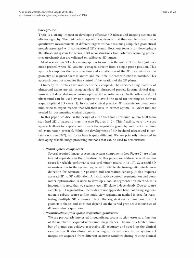
Figure 1 3D freehand ultrasound prototype system. The prototype system allows clinicians to optimizethe ultrasound acquisition geometry.


of 22

they are parallel to the ultrasound beam. In such cases, almost no echo energy

is reflected back to the transducer. These limitations can be addressed through

the use of multiple acoustic windows and views where the ultrasound beam can

propagate behind obstructions while imaging organ interfaces at the directions

that are not parallel to the ultrasound beam.

In our 3D freehand ultrasound prototype system, an electromagnetic position and

orientation measurement device (EPOM) is attached on a conventional 2D clinic ultra-

sound probe (see Figure 1). This allows 3D reconstruction from arbitrary sampling

geometries and multiple acoustic windows. It provides a simple hardware system that

allows for great flexibility in choosing suitable acoustic windows according to clinical

practice. Once a region of interest has been identified, a freehand 3D system allows

the experts to take very dense samples around the abnormality from an appropriate

acoustic window and view, providing very accurate reconstructions in the region of

interest.

Interest in the use of multiple views for providing 3D reconstructions has been pri-

marily focused on reconstructions of the left ventricle. Legget et al. [5] used a 2D free-

hand scanning protocol and manual registration to combine parasternal and apical

windows in-vitro. A similar system was reported by Leotta et al. [6]. Later, Ye et al. [7]

used a 3D rotational probe and an electromagnetic spatial locator to combine apical

long-axis view and parasternal short-axis view. The reconstructions are fused by fea-

tures and weighted by the image acquisition geometry. Reconstruction was limited by

the lack of automated registration. Good spatial alignment of the dense rotational

Figure 2 Software flow-chart for multi-view reconstructions from freehand 2D images. The softwaresystem allows us to measure the effects of interference, the use of a new hybrid segmentation and multi-view reconstruction with automated feature-based registration.


of 22

sweeps between different views was assumed. Long acquisition time for each view

(3-4 minutes in [7]) may result in unstable motion of the probe.

For ultrasound image registration, Rohling et. al. developed an automatic registration

method in gall bladder reconstruction [12]. Six, slightly different sweeps were collected

and the first sweep is used as baseline. Spatial compounding was performed by regis-

tering the last five sweeps to the first baseline based on the estimation of the cross-cor-

relation of 3D gradient magnitude [12] or the usage of landmarks [13]. A review of

cardiac image registration among multiple imaging modalities is available in [14]. As

stated in [15], due to the varied image quality associated with cardiac ultrasound

images, there are few publications focused on echocardiography image registration

[16-18]. Mutual information methods also presented difficulties associated with ultra-

sound image characteristics [19].

For real-time 3D echocardiography registration, Soler et al. [20] used manual marked

and segmented meshes of the left ventricle to register two different views from apical

window by intensity similarity measure. Grauet al. [15] registered parasternal and api-

cal views using phase and orientation similarity measures. Their method relied on the

use of manual landmark initialization. Here, we note that effective 3D ultrasound regis-

tration cannot be based on image intensity alone due to large intensity variations

within the same tissue structures and between the different views.

Unlike prior research based on the use of dense 3D samples, this paper is based on

the use of sparse 2D planes. We develop a fully-automated registration without manual

initialization. To the best of our knowledge, no such research has been reported in the

literature. To achieve reliable registration performance, we use a coarse to fine volu-

metric registration method. We initialize searching for the global optimal registration

parameters using a 3D Hotelling transform to construct a reference frame to coarsely

register 3D volumes from different acoustic windows. Then, feature-based high accu-

racy registration is performed using a robust, non-linear least squares algorithm.

Automatic feature segmentation is carried before multi-view registration. Automatic

segmentation techniques of echocardiographic images face a number of challenges due

to poor contrast, high-level speckle noise, weak endocardial boundaries and small

boundary gaps. Recently, promising segmentation results have been obtained using

methods based on deformable models. There are mainly parametric and geometric

deformable models [21]. In parametric models, the evolving segmentation curve is

explicitly represented. In geometric models, the evolving segmentation curve is impli-

citly expressed as level sets of a higher dimensional scalar function. Unlike parametric

models, geometric deformable models can handle topological changes automatically

and be easily extended to higher dimensional applications.

Parametric deformable models have been used in semi-automatic segmentation for

both the epicardial and endocardial borders over the entire cardiac cycle [22-24]. Here,

statistical models of the cardiac structure features (e.g. shape, intensity appearance and

temporal information) were derived from large training data sets for segmenting endo-

cardial boundaries [25-28]. For these methods, we note that there is significant over-

head associated with providing large and appropriate training data sets and also

significant efforts in setting up the point correspondences.

In clinical practice and especially in paediatric cardiology, there can be significantly

topological variability associated with ventricle wall boundaries. Due to the wide


of 22

variability in possible abnormal cases, it is difficult to provide significant populations

for each abnormal classification. This difficulty further limits the applicability of para-

metric model-based approaches. More recently, geometric level set models have been

developed to address these limitations. These models can handle topological changes

automatically without the need for extensive parameter training. Level set methods

have been used for echocardiography image segmentation [29]. Other variational level

set segmentation strategies also integrate prior knowledge (shape, statistical distribu-

tion etc.) [30-32]. However, the use of prior information often requires off-line training.

It can be tedious and expert-dependent.

Alternatively, Corsi et al. [33] developed a semi-automatic level set segmentation

method that did not require prior knowledge. The authors applied the method to real-

time 3D echocardiography images for reconstructing the left ventricle. In this study,

the initial surface had to be chosen close to the boundaries of the LV chamber.

We describe a new image segmentation method that relaxes the need for accurate

initialization. Here, we are proposing a two-step approach. After a rough initialization,

we first use a gradient vector flow (GVF) geodesic active contour (GAC) model to move

the initial contour closer to the true boundary. This is done by driving the initial con-

tour to the true boundary using strong GVF forces [34], which is integrated in geodesic

active contour (GAC) model [35-38]. Then, in the second step, the evolving curve is

driven by image gradient for accurate segmentation. It allows for relatively simple and

free initialisation of the model, while minimizing edge leaking. We also present a study

of the influence of the segmentation parameters on the model. To the best of our

knowledge, no similar parameter optimization is reported in publications in ultrasound

image segmentation.

The performance of the 3D system is demonstrated in its ability to provide accurate

volume estimates using sparse image plane sampling from multiple acoustic views. To

quantify accurate measures, the validation is focused on measures taken on calibrated

3D ultrasound phantoms. However, we also provide measures from in-vivo cardiac

data set.

MethodsHardware Setup and Software Flow Chart

For acquiring 2D ultrasound images, we use an Acuson Sequoia C256 (Siemens, USA)

with a 7 MHz array transducer probe 7V3C (see Figure 1). A six-degree of freedom

EPOM device, the Flock of Birds (FOB) (Ascension, Burlington, VT, USA) is used to

record 3D location of each 2D image. For accurate 3D reconstructions, a calibration

for determining the spatial relation between the sensor and the 2D images is per-

formed [4,39].

Figure 2 shows the system software flow chart. We start image acquisition with

breath-holding and ECG gating at the standard acoustic window. The purpose of

doing this is to avoid the cardiac deformation due to respiration and cyclic cardiac

motion. Then, the only significant source of misregistration is due to the rigid move-

ment of the patient. The position and orientation of the transducer associated with

each acquired 2D image (640 × 480) are saved in the computer. The region of interest

(ROI) is quickly outlined to reduce the computational and memory requirements. 2D

+T image sequences are segmented automatically to identify the endocardial


of 22

boundaries. The 3D surface of the LV is reconstructed with automated registration

using segmented boundary walls. The whole software is developed in C programming

language and MATLAB (MathWorks).

Hybrid Gradient Vector Flow (GVF) Geometric Active Contour (GAC) Model

Level sets segmentation allows the development of new image segmentation methods

that can adapt to complex object boundaries. We developed a new hybrid model that

can deliver accurate segmentation results from relatively simple initializations.

Level sets was first introduced by Osher and Sethian [40]. The authors started with a

model of a propagating front Γ(t) as the zero level set of a higher dimensional func-

tion: �(x,y,t). Initially, we have:

x y t d, , =( ) = ±0

where d is the signed distance from point (x,y) to the boundary of an region Ω (Γ(t)

bounds the region Ω) at t = 0. If d = 0, the point (x,y) is on the boundary. For points

that are inside the initial boundary, �(x,y,t = 0) takes on negative values. For points

that are outside the initial boundary, �(x,y,t = 0) takes on positive values.

Osher and Sethian [40] had shown that �(x,y,t) evolves according to the following

dynamic equation:

∂∂

+ ⋅ ∇ =

tF

0

with the initial condition �(x,y,0) = �0 (x,y).F is the propagation velocity function

on the interface. Here, only the normal component ofF is needed. The unit normal

vector (outward) to the level set curve is given by:

n

= ∇∇

.

The evolution equation becomes

∂∂

+ ⋅ ∇ =

tF 0

Where F is the normal component ofF , given by

F F= ⋅ ∇∇

=

0

For image segmentation applications, the goal is to design the speed function F so as

to propagate the evolving curve to the edges of the image. There are three main types

of motion in curve evolution [41]. We write as:

F F F Fnorm curv adv= + +

where Fnorm denotes motion in the normal direction; Fcurv denotes motion in the

curvature direction, and Fadvdenotes motion due to an externally generated velocity

field, independent of the front itself.


of 22

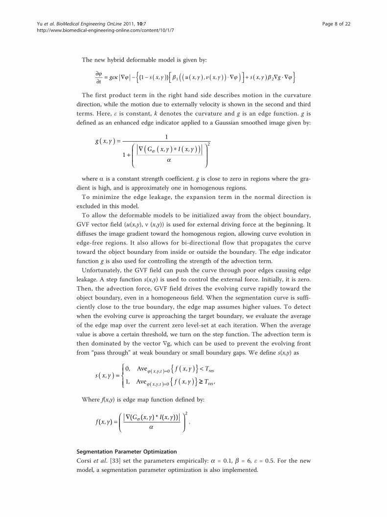
The new hybrid deformable model is given by:

∂∂

= ∇ − − ( ) ( ) ( )( ) ⋅ ∇( )⎡⎣

⎤⎦ + ( ) ∇

t

g s x y u x y v x y s x y g( , ) , , , ,1 1 2 ⋅⋅ ∇{ }The first product term in the right hand side describes motion in the curvature

direction, while the motion due to externally velocity is shown in the second and third

terms. Here, ε is constant, k denotes the curvature and g is an edge function. g is

defined as an enhanced edge indicator applied to a Gaussian smoothed image given by:

g x yG x y I x y

,, ,

( ) =

+∇ ( ) ∗ ( )( )⎛

⎝

⎜⎜

⎞

⎠

⎟⎟

1

1

2

where a is a constant strength coefficient. g is close to zero in regions where the gra-

dient is high, and is approximately one in homogenous regions.

To minimize the edge leakage, the expansion term in the normal direction is

excluded in this model.

To allow the deformable models to be initialized away from the object boundary,

GVF vector field (u(x,y), ν (x,y)) is used for external driving force at the beginning. It

diffuses the image gradient toward the homogenous region, allowing curve evolution in

edge-free regions. It also allows for bi-directional flow that propagates the curve

toward the object boundary from inside or outside the boundary. The edge indicator

function g is also used for controlling the strength of the advection term.

Unfortunately, the GVF field can push the curve through poor edges causing edge

leakage. A step function s(x,y) is used to control the external force. Initially, it is zero.

Then, the advection force, GVF field drives the evolving curve rapidly toward the

object boundary, even in a homogeneous field. When the segmentation curve is suffi-

ciently close to the true boundary, the edge map assumes higher values. To detect

when the evolving curve is approaching the target boundary, we evaluate the average

of the edge map over the current zero level-set at each iteration. When the average

value is above a certain threshold, we turn on the step function. The advection term is

then dominated by the vector ∇g, which can be used to prevent the evolving front

from “pass through” at weak boundary or small boundary gaps. We define s(x,y) as

s x yf x y T

f x y

x y t res

x y t

,, Ave ,

, Ave ,

, ,

, ,

( ) =( ){ } <

( ){ }( )=

( )=

0

1

0

0

≥≥

⎧⎨⎪

⎩⎪ Tres ,

Where f(x,y) is edge map function defined by:

f x yG x y I x y

( , )( ( , )* ( , ))

.=∇⎛

⎝⎜⎜

⎞

⎠⎟⎟

2

Segmentation Parameter Optimization

Corsi et al. [33] set the parameters empirically: a = 0.1, b = 6, ε = 0.5. For the new

model, a segmentation parameter optimization is also implemented.


of 22

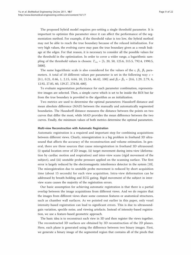
The proposed hybrid model requires pre-setting a single threshold parameter. It is

important to optimize this parameter since it can affect the performance of the seg-

mentation method. For example, if the threshold value is too low, the hybrid method

may not be able to reach the true boundary because of the relaxed initialization. For

very high values, the evolving curve may pass the true boundary given as a result leak-

age at the edges. For that reason, it is necessary to consider all the possible values for

the threshold in the optimization. In order to cover a wider range, a logarithmic sam-

pling of the threshold values is chosen: Tres = [5, 20, 50, 125.6, 315.5, 792.4, 1990.5,

5000].

The same logarithmic scale is also considered for the values of the ε, b1, b2 para-

meters. A total of 10 different values per parameter is set in the following way: ε =

[0.1, 0.21, 0.46, 1, 2.15, 4.64, 10, 21.54, 46.42, 100] and b1= b2 = [0.6, 1.29, 2.79, 6,

12.92, 27.85, 60, 129.27, 278.50, 600].

To evaluate segmentation performance for each parameter combination, representa-

tive images are selected. Then, a simple curve which is set to be inside the ROI but far

from the true boundary is provided to the algorithm as an initialization.

Two metrics are used to determine the optimal parameters: Hausdorff distance and

mean absolute difference (MAD) between the manually and automatically segmented

boundaries. The Hausdorff distance measures the distance between the points on two

curves that differ the most, while MAD provides the mean difference between the two

curves. Finally, the minimum values of both metrics determine the optimal parameters.

Multi-view Reconstruction with Automatic Registration

Automatic registration is a required and important step for combining acquisitions

between different views. Clearly, misregistration is a big problem in freehand 3D ultra-

sound that affects the accuracy of the reconstruction and volume estimation. In gen-

eral, there are three sources that cause misregistration in freehand 3D ultrasound:

(i) spatial location error of 2D image, (ii) target movement during intra-view (deforma-

tion by cardiac motion and respiration) and inter-view scans (rigid movement of the

subject), and (iii) unstable probe pressure applied on the scanning surface. The first

error is largely reduced by the electromagnetic interference detector in the system [10].

The misregistration due to unstable probe movement is reduced by short acquisition

time (about 15 seconds) for each view acquisition. Intra-view deformation can be

addressed by breath-holding and ECG gating. Rigid movement of the subject in inter-

view scans causes the majority of the registration errors.

Our basic assumption for achieving automatic registration is that there is a partial

overlap between the image acquisitions from different views. And we do require that

the images from different views share some common features or anatomical structures,

such as chamber wall surfaces. As we pointed out earlier in this paper, only voxel

intensity-based registration can lead to significant errors. This is due to ultrasound-

gain variation, speckle noise, and viewing artefacts. Instead of intensity-based registra-

tion, we use a feature-based geometric approach.

The basic idea is to reconstruct each view in 3D and then register the views together.

The reconstructed 3D surfaces are obtained by 3D reconstruction of the 2D planes.

Here, each plane is generated using the difference between two binary images. First,

we generate a binary image of the segmented region that contains all of the pixels that


of 22

fall inside the object of interest. The second binary image is generated by eroding the

first one using a circular element of radius of 4 to 8 pixels (based on target size). The

difference image captures the boundary wall. A 3D reconstruction of the 2D planes

generates a 3D binary surface model.

We note that registration is possible as long as the reconstructed wall surfaces exhi-

bit some overlap. To satisfy the partial overlap criterion, we require that at-least one of

the views is a full-sweep, covering the entire object of interest. We expect that the

inherent appearances of chamber wall surfaces will guarantee the existence of a unique

global minimum for the registration parameters.

To reach the globally optimal value, we first apply a global registration method by

using 3D Hotelling transform to construct an object-based reference volume. This is

needed to avoid local minima and ensure a significant overlap between different view

acquisitions. Then, we perform a higher accuracy registration using a robust, non-

linear least squares algorithm to archive the optimal parameters.

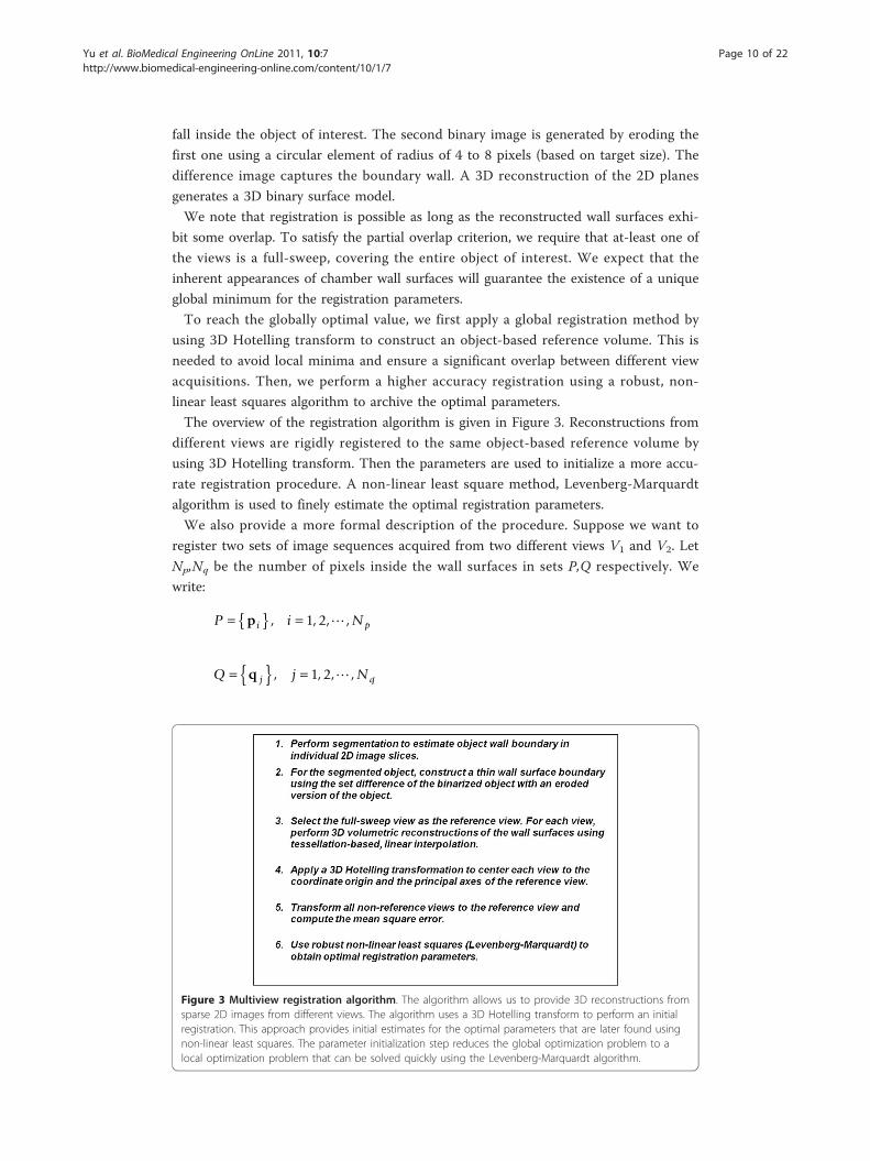
The overview of the registration algorithm is given in Figure 3. Reconstructions from

different views are rigidly registered to the same object-based reference volume by

using 3D Hotelling transform. Then the parameters are used to initialize a more accu-

rate registration procedure. A non-linear least square method, Levenberg-Marquardt

algorithm is used to finely estimate the optimal registration parameters.

We also provide a more formal description of the procedure. Suppose we want to

register two sets of image sequences acquired from two different views V1 and V2. Let

Np,Nq be the number of pixels inside the wall surfaces in sets P,Q respectively. We

write:

P i Ni p= { } =p , , , ,1 2

Q j Nj q= { } =q , , , ,1 2

Figure 3 Multiview registration algorithm. The algorithm allows us to provide 3D reconstructions fromsparse 2D images from different views. The algorithm uses a 3D Hotelling transform to perform an initialregistration. This approach provides initial estimates for the optimal parameters that are later found usingnon-linear least squares. The parameter initialization step reduces the global optimization problem to alocal optimization problem that can be solved quickly using the Levenberg-Marquardt algorithm.


of 22

where pi,qj are 3D voxel coordinates from the two views:

p i i i iT

x y z= [ ], ,

q j j j jT

x y z= ⎡⎣ ⎤⎦, , .

We then reconstruct the 3D volume with the largest number of 2D image planes (for

example, view V1 ) over a regular Cartesian grid, and then register the 2D image slices

from the rest of the views (for example, view V2) to it.

The data points from the second view V2 are transformed using the initial transfor-

mation acquired using 3D Hotelling, denoted as T(qj). We interpolate the intensity

values at T(qj) using the image points of I(pi) in 3D Cartesian grid volume. The opti-

mal registration transformation is obtained as the one that minimizes the mean square

error of the objective function:

f P T Qn T

I p I T qR i N j

p q O Ti j

, ( )( )

, ( )

( ) = ( ) − ( )( )⎡⎣⎢

⎤⎦⎥

∈∑1 2

where O is the overlapping region between the two volumes, IR refers to the refer-

ence 3D reconstruction, IN refers to the “new” 3D reconstruction to register, and n is

the number of the voxels within set O. Once the images are registered, the 3D recon-

structed volume is achieved by averaging the intensities from the different view

volumes to attenuate artefacts and reduce noise.

ResultsData Sets and Acquisition

The system is evaluated on calibrated 3D ultrasound phantom and in-vivo paediatric

cardiac data set. We use the standard 3D calibration phantom (Model 055, CIRS,

USA) which contains two volumetric egg-shape objects that can be scanned from both

top and the side windows. From each scanning window, ultrasound images can be col-

lected at both the long-axis and short-axis views. Eight sequences of phantom image

videos are used for validating single view and multi-view reconstructions. The numbers

of images in each view reconstruction are shown in Table 1.

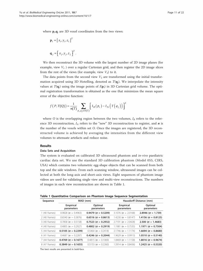
Table 1 Quantitative Comparison on Phantom Image Sequence Segmentation

Sequence MAD (mm) Hausdorff Distance (mm)

Empiricalparameters

Optimalparameters

Empiricalparameters

Optimalparameters

1 (40 frames) 0.9828 (s = 0.4963) 0.9479 (s = 0.5209) 3.1076 (s = 2.0168) 2.8946 (s = 1.739)

2 (40 frames) 0.6540 (s = 0.3876) 0.6516 (s = 0.8613) 1.4230 (s = 0.8147) 1.4156 (s = 0.8125)

3 (40 frames) 0.7858 (s = 0.5158) 0.7523 (s = 0.2932) 2.7191 (s = 2.0428) 2.500 (s = 1.4683)

4 (40 frames) 0.4805 (s = 0.2927) 0.4802 (s = 0.2919) 1.1981 (s = 0.7535) 1.1971 (s = 0.7504)

5 (44 frames) 0.5105 (s = 0.2299) 0.5464 (s = 0.2418) 2.1746 (s = 1.1174) 1.6694 (s = 0.8680)

6 (41 frames) 0.4687 (s = 0.2287) 0.4246 (s = 0.2044) 1.9629 (s = 0.9913) 1.0510 (s = 0.5140)

7 (44 frames) 0.4769 (s = 0.1677) 0.4815 (s = 0.1069) 1.8469 (s = 1.1158) 1.8016 (s = 0.9674)

8 (47 frames) 0.3849 (s = 0.1655) 0.5153 (s = 0.2260) 1.5914 (s = 0.8436) 1.2425 (s = 0.5320)

The best results are presented in bold-face.


of 22

While most of the current research has focused on adult cardiology, our primary

focus here has been on applications in paediatric cardiology. In paediatric echocardio-

graphy, smaller heart size, higher heart rate, and more complicated cardiac anatomy

make accurate 3D reconstruction even harder.

Four sequences of in-vivo paediatric cardiac image videos are used in the cardiac

experiment. Data sets are acquired from the parasternal short-axis view and the apical

long-axis view from a six year old healthy child volunteer. Breath holding (15 seconds)

and ECG gating are used to minimize the deformation from respiration and cardiac

motion. In each view acquisition, the transducer is moved slowly and evenly to scan

the heart. Due to the standard frame rate of the frame grabber (nearly 30 frames per

second), 433 images with 640 × 480 resolution are collected in 15 seconds, which is a

much shorter scanning time than the acquisition time reported by Ye et al. [7]. The

subject does not have to remain still during the time it takes to switch to a different

acoustic window. The image acquisition procedure for 3D is done exactly in the same

way as the regular routine echocardiography examination at the hospital.

Segmentation

Two typical ultrasound images (a phantom image and a cardiac image) for estimating

the optimal segmentation parameters are selected. Figures 4 and 5 show the images

used in the optimization and their results. Hausdorff distance and MAD are used to

measure the difference between the manual and automatic segmentation boundaries.

Similar results are obtained when optimising for the minimal Hausdorff distance or

MAD. In what follows, we present and discuss results for the Hausdorff distance.

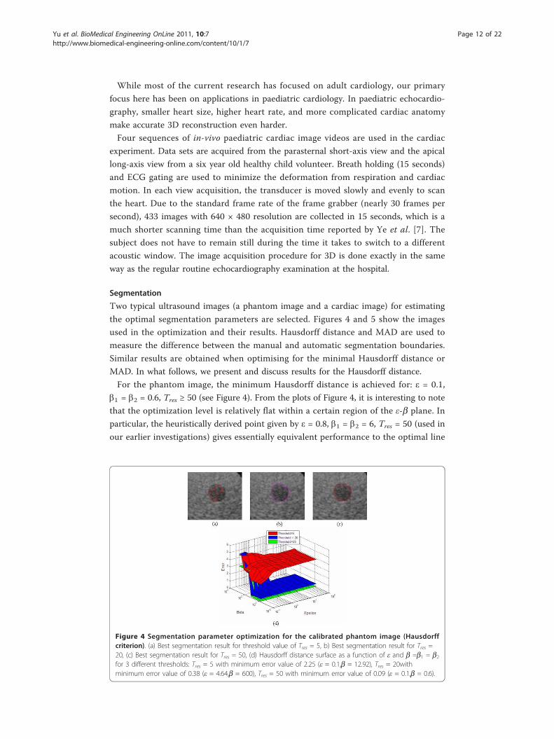
For the phantom image, the minimum Hausdorff distance is achieved for: ε = 0.1,

b1 = b2 = 0.6, Tres ≥ 50 (see Figure 4). From the plots of Figure 4, it is interesting to note

that the optimization level is relatively flat within a certain region of the ε-b plane. In

particular, the heuristically derived point given by ε = 0.8, b1 = b2 = 6, Tres = 50 (used in

our earlier investigations) gives essentially equivalent performance to the optimal line

Figure 4 Segmentation parameter optimization for the calibrated phantom image (Hausdorffcriterion). (a) Best segmentation result for threshold value of Tres = 5, b) Best segmentation result for Tres =20, (c) Best segmentation result for Tres = 50, (d) Hausdorff distance surface as a function of ε and b =b1 = b2for 3 different thresholds: Tres = 5 with minimum error value of 2.25 (ε = 0.1,b = 12.92), Tres = 20withminimum error value of 0.38 (ε = 4.64,b = 600), Tres = 50 with minimum error value of 0.09 (ε = 0.1,b = 0.6).


of 22

given by ε = 0.1, b1 = b2 = 0.6, Tres ≥ 50. To minimize computational complexity, we use

the point given Tres = 50. It allows for the evolving front to converge quickly under GVF

force to the region around the boundary, before it allows for local gradient to slowly

fine-tune the final result. Here, the optimal results require that b values be at-least six

times larger than the ε value where ε lies in the interval of [0.1, 100].

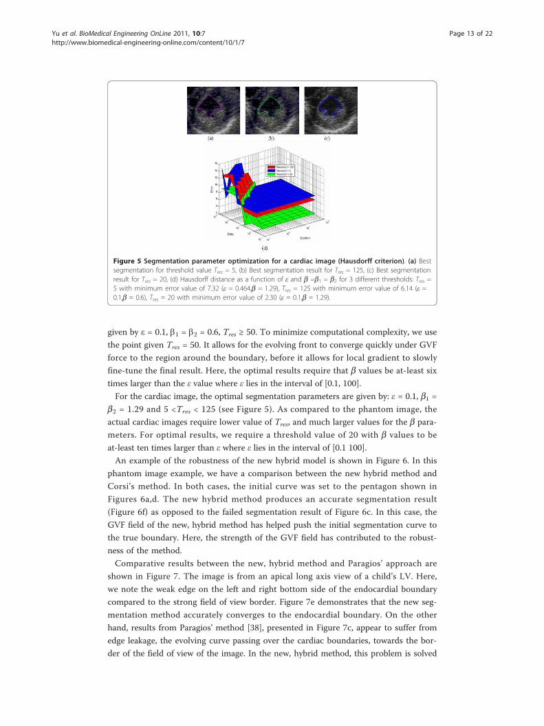
For the cardiac image, the optimal segmentation parameters are given by: ε = 0.1, b1 =b2 = 1.29 and 5 <Tres < 125 (see Figure 5). As compared to the phantom image, the

actual cardiac images require lower value of Tres, and much larger values for the b para-

meters. For optimal results, we require a threshold value of 20 with b values to be

at-least ten times larger than ε where ε lies in the interval of [0.1 100].

An example of the robustness of the new hybrid model is shown in Figure 6. In this

phantom image example, we have a comparison between the new hybrid method and

Corsi’s method. In both cases, the initial curve was set to the pentagon shown in

Figures 6a,d. The new hybrid method produces an accurate segmentation result

(Figure 6f) as opposed to the failed segmentation result of Figure 6c. In this case, the

GVF field of the new, hybrid method has helped push the initial segmentation curve to

the true boundary. Here, the strength of the GVF field has contributed to the robust-

ness of the method.

Comparative results between the new, hybrid method and Paragios’ approach are

shown in Figure 7. The image is from an apical long axis view of a child’s LV. Here,

we note the weak edge on the left and right bottom side of the endocardial boundary

compared to the strong field of view border. Figure 7e demonstrates that the new seg-

mentation method accurately converges to the endocardial boundary. On the other

hand, results from Paragios’ method [38], presented in Figure 7c, appear to suffer from

edge leakage, the evolving curve passing over the cardiac boundaries, towards the bor-

der of the field of view of the image. In the new, hybrid method, this problem is solved

Figure 5 Segmentation parameter optimization for a cardiac image (Hausdorff criterion). (a) Bestsegmentation for threshold value Tres = 5, (b) Best segmentation result for Tres = 125, (c) Best segmentationresult for Tres = 20, (d) Hausdorff distance as a function of ε and b =b1 = b2 for 3 different thresholds: Tres =5 with minimum error value of 7.32 (ε = 0.464,b = 1.29), Tres = 125 with minimum error value of 6.14 (ε =0.1,b = 0.6), Tres = 20 with minimum error value of 2.30 (ε = 0.1,b = 1.29).


of 22

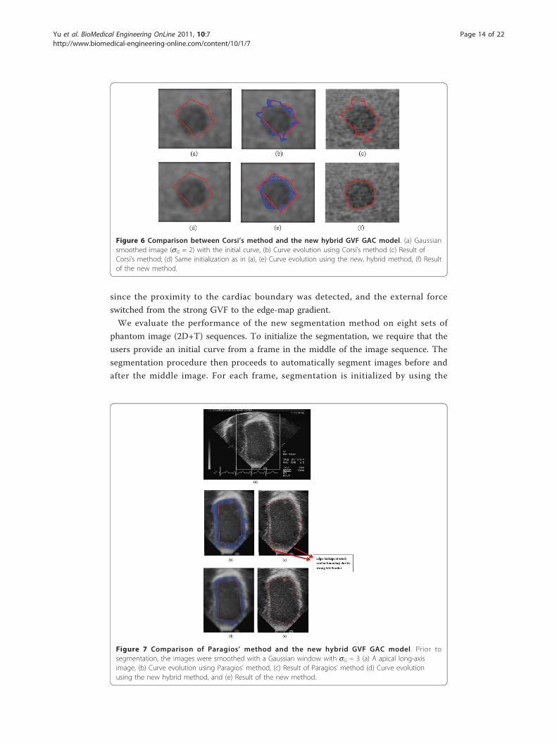
since the proximity to the cardiac boundary was detected, and the external force

switched from the strong GVF to the edge-map gradient.

We evaluate the performance of the new segmentation method on eight sets of

phantom image (2D+T) sequences. To initialize the segmentation, we require that the

users provide an initial curve from a frame in the middle of the image sequence. The

segmentation procedure then proceeds to automatically segment images before and

after the middle image. For each frame, segmentation is initialized by using the

Figure 7 Comparison of Paragios’ method and the new hybrid GVF GAC model . Prior tosegmentation, the images were smoothed with a Gaussian window with sG = 3 (a) A apical long-axisimage, (b) Curve evolution using Paragios’ method, (c) Result of Paragios’ method (d) Curve evolutionusing the new hybrid method, and (e) Result of the new method.

Figure 6 Comparison between Corsi’s method and the new hybrid GVF GAC model. (a) Gaussiansmoothed image (sG = 2) with the initial curve, (b) Curve evolution using Corsi’s method (c) Result ofCorsi’s method; (d) Same initialization as in (a), (e) Curve evolution using the new, hybrid method, (f) Resultof the new method.


of 22

segmented curve from the previous frame, allowing for a quick convergence and accu-

rate segmentation.

In order to discuss the effects of the segmentation parameters, we present results for

both optimized and non-optimized (empirical) segmentation. For the non-optimized

segmentation, we set the parameters empirically, after a few experiments with a couple

of training images (ε = 0.8, b1 = b2 = 6, Tres = 50). For the optimized results, we follow

the optimization method that we described in the Methods Section.

Table 1 shows that the optimal parameters gave the lowest Hausdorff distance errors

in all cases. For the MAD, the optimized approach gives the best results in the major-

ity of the cases. On average, the MAD stays below 1mm while the maximum segmen-

tation error stays below 3mm (Hausdorff distance). It is interesting to note that there

is more consistency in the optimized approach, in the sense that the standard devia-

tions of the Hausdorff distances is found to be remain lower than the empirical

approach.

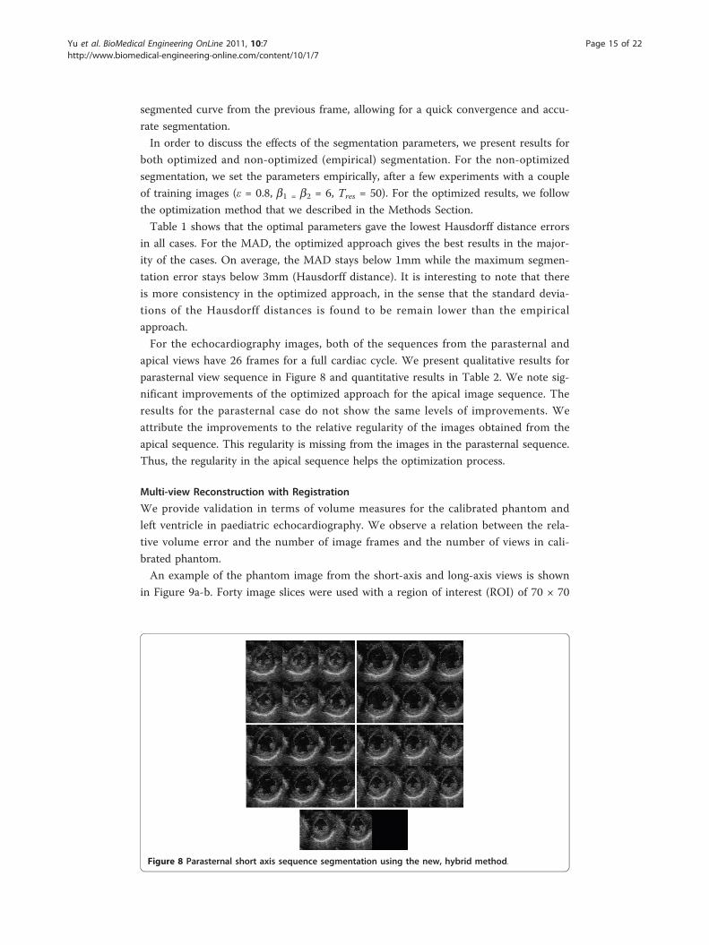
For the echocardiography images, both of the sequences from the parasternal and

apical views have 26 frames for a full cardiac cycle. We present qualitative results for

parasternal view sequence in Figure 8 and quantitative results in Table 2. We note sig-

nificant improvements of the optimized approach for the apical image sequence. The

results for the parasternal case do not show the same levels of improvements. We

attribute the improvements to the relative regularity of the images obtained from the

apical sequence. This regularity is missing from the images in the parasternal sequence.

Thus, the regularity in the apical sequence helps the optimization process.

Multi-view Reconstruction with Registration

We provide validation in terms of volume measures for the calibrated phantom and

left ventricle in paediatric echocardiography. We observe a relation between the rela-

tive volume error and the number of image frames and the number of views in cali-

brated phantom.

An example of the phantom image from the short-axis and long-axis views is shown

in Figure 9a-b. Forty image slices were used with a region of interest (ROI) of 70 × 70

Figure 8 Parasternal short axis sequence segmentation using the new, hybrid method.


of 22

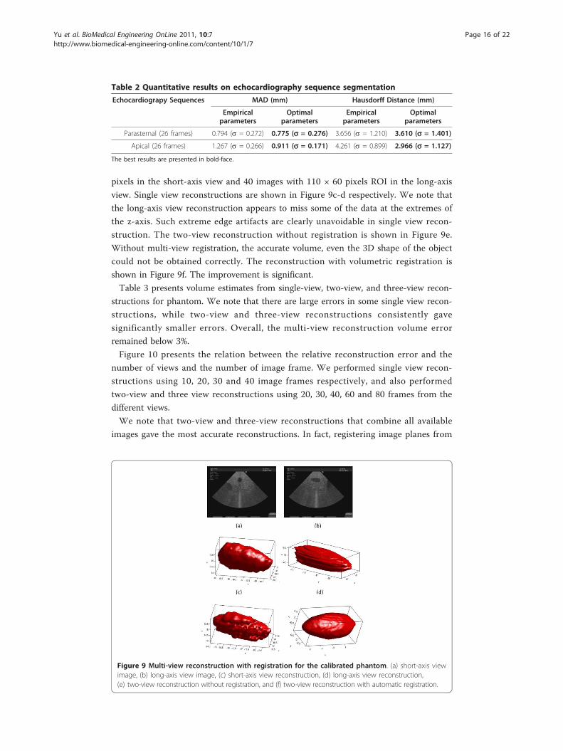
pixels in the short-axis view and 40 images with 110 × 60 pixels ROI in the long-axis

view. Single view reconstructions are shown in Figure 9c-d respectively. We note that

the long-axis view reconstruction appears to miss some of the data at the extremes of

the z-axis. Such extreme edge artifacts are clearly unavoidable in single view recon-

struction. The two-view reconstruction without registration is shown in Figure 9e.

Without multi-view registration, the accurate volume, even the 3D shape of the object

could not be obtained correctly. The reconstruction with volumetric registration is

shown in Figure 9f. The improvement is significant.

Table 3 presents volume estimates from single-view, two-view, and three-view recon-

structions for phantom. We note that there are large errors in some single view recon-

structions, while two-view and three-view reconstructions consistently gave

significantly smaller errors. Overall, the multi-view reconstruction volume error

remained below 3%.

Figure 10 presents the relation between the relative reconstruction error and the

number of views and the number of image frame. We performed single view recon-

structions using 10, 20, 30 and 40 image frames respectively, and also performed

two-view and three view reconstructions using 20, 30, 40, 60 and 80 frames from the

different views.

We note that two-view and three-view reconstructions that combine all available

images gave the most accurate reconstructions. In fact, registering image planes from

Table 2 Quantitative results on echocardiography sequence segmentation

Echocardiograpy Sequences MAD (mm) Hausdorff Distance (mm)

Empiricalparameters

Optimalparameters

Empiricalparameters

Optimalparameters

Parasternal (26 frames) 0.794 (s = 0.272) 0.775 (s = 0.276) 3.656 (s = 1.210) 3.610 (s = 1.401)

Apical (26 frames) 1.267 (s = 0.266) 0.911 (s = 0.171) 4.261 (s = 0.899) 2.966 (s = 1.127)

The best results are presented in bold-face.

Figure 9 Multi-view reconstruction with registration for the calibrated phantom. (a) short-axis viewimage, (b) long-axis view image, (c) short-axis view reconstruction, (d) long-axis view reconstruction,(e) two-view reconstruction without registration, and (f) two-view reconstruction with automatic registration.


of 22

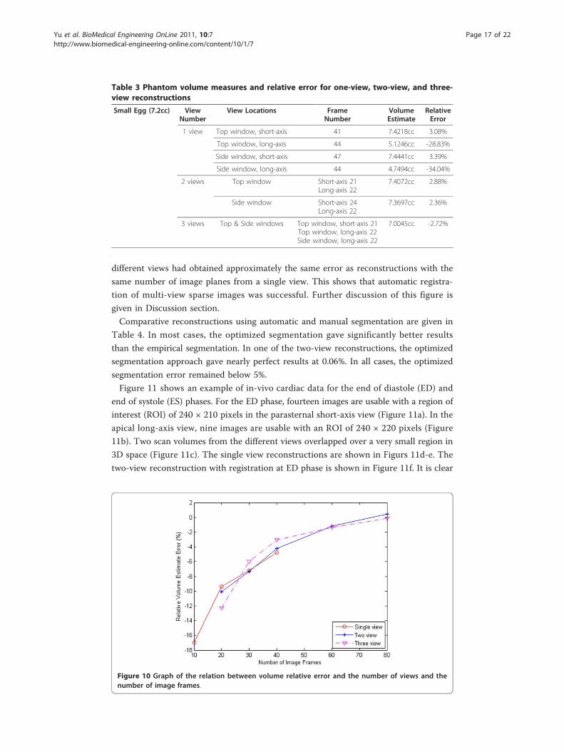
different views had obtained approximately the same error as reconstructions with the

same number of image planes from a single view. This shows that automatic registra-

tion of multi-view sparse images was successful. Further discussion of this figure is

given in Discussion section.

Comparative reconstructions using automatic and manual segmentation are given in

Table 4. In most cases, the optimized segmentation gave significantly better results

than the empirical segmentation. In one of the two-view reconstructions, the optimized

segmentation approach gave nearly perfect results at 0.06%. In all cases, the optimized

segmentation error remained below 5%.

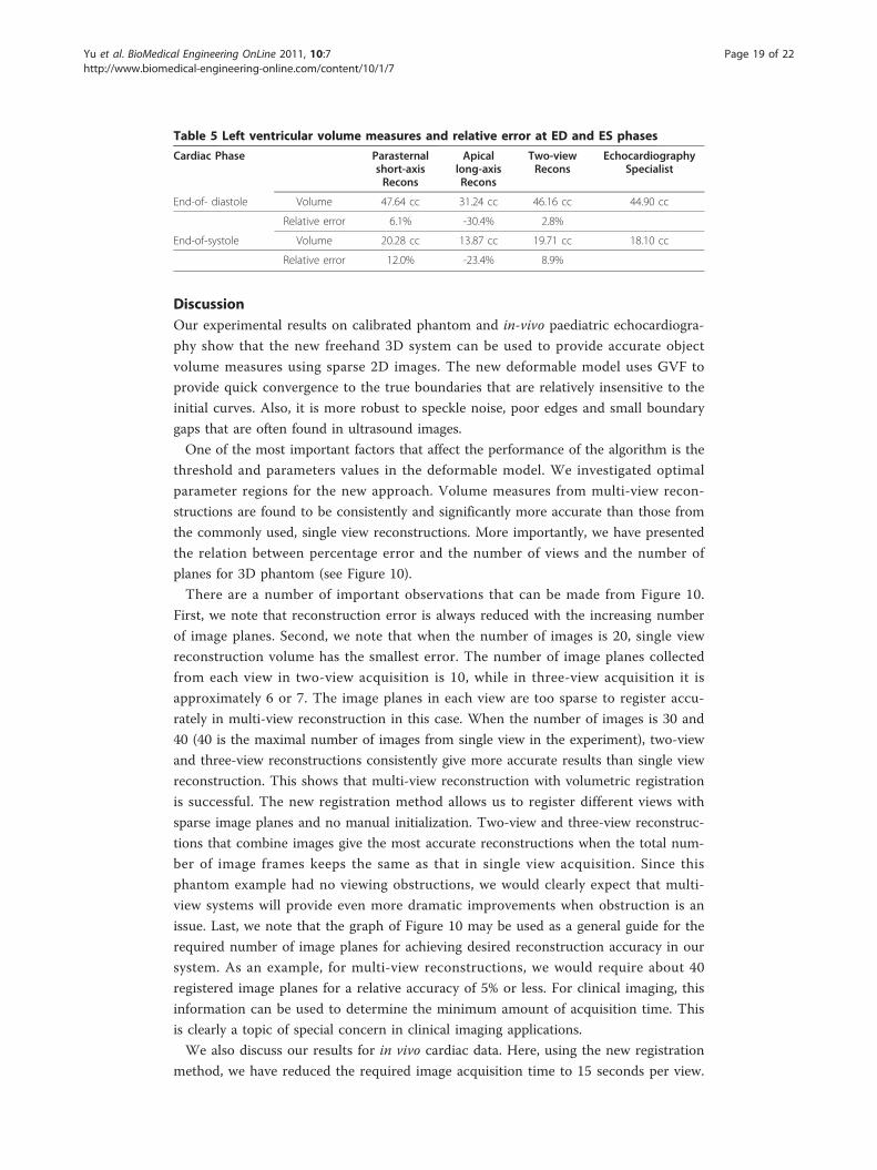
Figure 11 shows an example of in-vivo cardiac data for the end of diastole (ED) and

end of systole (ES) phases. For the ED phase, fourteen images are usable with a region of

interest (ROI) of 240 × 210 pixels in the parasternal short-axis view (Figure 11a). In the

apical long-axis view, nine images are usable with an ROI of 240 × 220 pixels (Figure

11b). Two scan volumes from the different views overlapped over a very small region in

3D space (Figure 11c). The single view reconstructions are shown in Figurs 11d-e. The

two-view reconstruction with registration at ED phase is shown in Figure 11f. It is clear

Table 3 Phantom volume measures and relative error for one-view, two-view, and three-view reconstructions

Small Egg (7.2cc) ViewNumber

View Locations FrameNumber

VolumeEstimate

RelativeError

1 view Top window, short-axis 41 7.4218cc 3.08%

Top window, long-axis 44 5.1246cc -28.83%

Side window, short-axis 47 7.4441cc 3.39%

Side window, long-axis 44 4.7494cc -34.04%

2 views Top window Short-axis 21Long-axis 22

7.4072cc 2.88%

Side window Short-axis 24Long-axis 22

7.3697cc 2.36%

3 views Top & Side windows Top window, short-axis 21Top window, long-axis 22Side window, long-axis 22

7.0045cc -2.72%

Figure 10 Graph of the relation between volume relative error and the number of views and thenumber of image frames.


of 22

that the two-view reconstruction combined the information from the two different views

and gave a more comprehensive and better result.

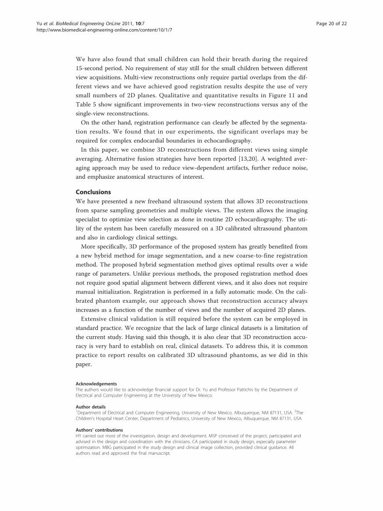
The quantitative results is shown in Table 5, the two-view reconstruction is in much

better agreement with the echocardiography specialist measures, with a relative error

of 2.8% in ED phase (see [11] for clinical measure approach). Here, we use the same

number of image planes and ROI-sizes for the ES phase and had similar results for the

two-view reconstruction at the ES phase. The two-view reconstruction of Figure 11g

gave a relative error of 8.9% at the ES phase, which is significantly lower than that

from single-view reconstructions.

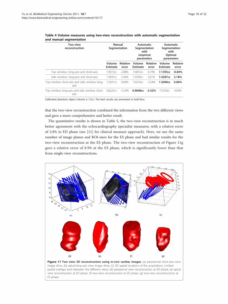
Table 4 Volume measures using two-view reconstruction with automatic segmentationand manual segmentation

Two-viewreconstruction

ManualSegmentation

AutomaticSegmentation

withempiricalparameters

AutomaticSegmentation

withOptimal

parameters

VolumeEstimate

Relativeerror

VolumeEstimate

Relativeerror

VolumeEstimate

Relativeerror

Top window: long-axis and short-axis 7.4072cc 2.88% 7.6853cc 6.74% 7.1395cc -0.84%

Side window: long-axis and short-axis 7.3697cc 2.36% 7.4599cc 3.61% 7.4287cc 3.18%

Top window short-axis and side window long-axis

7.2431cc 0.60% 7.0314cc -2.34% 7.2040cc 0.06%

Top window long-axis and side window short-axis

6.8225cc -5.24% 6.9608cc -3.32% 7.5376cc 4.69%

Calibrated phantom object volume is 7.2cc. The best results are presented in bold-face.

Figure 11 Two view 3D reconstruction using in-vivo cardiac images. (a) parasternal short-axis viewimage slices, (b) apical-long axis view image slices, (c) 3D spatial locations of the acquisitions. Limitedpartial overlaps exist between the different views, (d) parasternal view reconstruction at ED phase, (e) apicalview reconstruction at ED phase. (f) two-view reconstruction at ED phase, (g) two-view reconstructions atES phase.


of 22

DiscussionOur experimental results on calibrated phantom and in-vivo paediatric echocardiogra-

phy show that the new freehand 3D system can be used to provide accurate object

volume measures using sparse 2D images. The new deformable model uses GVF to

provide quick convergence to the true boundaries that are relatively insensitive to the

initial curves. Also, it is more robust to speckle noise, poor edges and small boundary

gaps that are often found in ultrasound images.

One of the most important factors that affect the performance of the algorithm is the

threshold and parameters values in the deformable model. We investigated optimal

parameter regions for the new approach. Volume measures from multi-view recon-

structions are found to be consistently and significantly more accurate than those from

the commonly used, single view reconstructions. More importantly, we have presented

the relation between percentage error and the number of views and the number of

planes for 3D phantom (see Figure 10).

There are a number of important observations that can be made from Figure 10.

First, we note that reconstruction error is always reduced with the increasing number

of image planes. Second, we note that when the number of images is 20, single view

reconstruction volume has the smallest error. The number of image planes collected

from each view in two-view acquisition is 10, while in three-view acquisition it is

approximately 6 or 7. The image planes in each view are too sparse to register accu-

rately in multi-view reconstruction in this case. When the number of images is 30 and

40 (40 is the maximal number of images from single view in the experiment), two-view

and three-view reconstructions consistently give more accurate results than single view

reconstruction. This shows that multi-view reconstruction with volumetric registration

is successful. The new registration method allows us to register different views with

sparse image planes and no manual initialization. Two-view and three-view reconstruc-

tions that combine images give the most accurate reconstructions when the total num-

ber of image frames keeps the same as that in single view acquisition. Since this

phantom example had no viewing obstructions, we would clearly expect that multi-

view systems will provide even more dramatic improvements when obstruction is an

issue. Last, we note that the graph of Figure 10 may be used as a general guide for the

required number of image planes for achieving desired reconstruction accuracy in our

system. As an example, for multi-view reconstructions, we would require about 40

registered image planes for a relative accuracy of 5% or less. For clinical imaging, this

information can be used to determine the minimum amount of acquisition time. This

is clearly a topic of special concern in clinical imaging applications.

We also discuss our results for in vivo cardiac data. Here, using the new registration

method, we have reduced the required image acquisition time to 15 seconds per view.

Table 5 Left ventricular volume measures and relative error at ED and ES phases

Cardiac Phase Parasternalshort-axisRecons

Apicallong-axisRecons

Two-viewRecons

EchocardiographySpecialist

End-of- diastole Volume 47.64 cc 31.24 cc 46.16 cc 44.90 cc

Relative error 6.1% -30.4% 2.8%

End-of-systole Volume 20.28 cc 13.87 cc 19.71 cc 18.10 cc

Relative error 12.0% -23.4% 8.9%


of 22

We have also found that small children can hold their breath during the required

15-second period. No requirement of stay still for the small children between different

view acquisitions. Multi-view reconstructions only require partial overlaps from the dif-

ferent views and we have achieved good registration results despite the use of very

small numbers of 2D planes. Qualitative and quantitative results in Figure 11 and

Table 5 show significant improvements in two-view reconstructions versus any of the

single-view reconstructions.

On the other hand, registration performance can clearly be affected by the segmenta-

tion results. We found that in our experiments, the significant overlaps may be

required for complex endocardial boundaries in echocardiography.

In this paper, we combine 3D reconstructions from different views using simple

averaging. Alternative fusion strategies have been reported [13,20]. A weighted aver-

aging approach may be used to reduce view-dependent artifacts, further reduce noise,

and emphasize anatomical structures of interest.

ConclusionsWe have presented a new freehand ultrasound system that allows 3D reconstructions

from sparse sampling geometries and multiple views. The system allows the imaging

specialist to optimize view selection as done in routine 2D echocardiography. The uti-

lity of the system has been carefully measured on a 3D calibrated ultrasound phantom

and also in cardiology clinical settings.

More specifically, 3D performance of the proposed system has greatly benefited from

a new hybrid method for image segmentation, and a new coarse-to-fine registration

method. The proposed hybrid segmentation method gives optimal results over a wide

range of parameters. Unlike previous methods, the proposed registration method does

not require good spatial alignment between different views, and it also does not require

manual initialization. Registration is performed in a fully automatic mode. On the cali-

brated phantom example, our approach shows that reconstruction accuracy always

increases as a function of the number of views and the number of acquired 2D planes.

Extensive clinical validation is still required before the system can be employed in

standard practice. We recognize that the lack of large clinical datasets is a limitation of

the current study. Having said this though, it is also clear that 3D reconstruction accu-

racy is very hard to establish on real, clinical datasets. To address this, it is common

practice to report results on calibrated 3D ultrasound phantoms, as we did in this

paper.

AcknowledgementsThe authors would like to acknowledge financial support for Dr. Yu and Professor Pattichis by the Department ofElectrical and Computer Engineering at the University of New Mexico.

Author details1Department of Electrical and Computer Engineering, University of New Mexico, Albuquerque, NM 87131, USA. 2TheChildren’s Hospital Heart Center, Department of Pediatrics, University of New Mexico, Albuquerque, NM 87131, USA.

Authors’ contributionsHY carried out most of the investigation, design and development. MSP conceived of the project, participated andadvised in the design and coordination with the clinicians. CA participated in study design, especially parameteroptimization. MBG participated in the study design and clinical image collection, provided clinical guidance. Allauthors read and approved the final manuscript.


of 22

Competing interestsThe authors declare that they have no competing interests.

Received: 7 October 2010 Accepted: 20 January 2011 Published: 20 January 2011

References1. Vieyres P, Poisson G, Courrèges F, Smith-Guerin N, Novales C, Arbeille P: A Tele-operated Robotic System for Mobile

Tele-echography: The OTELO Project. In M-Health: Emerging Mobile Health Systems Edited by: Istepanian RH,Laxminarayan S, Pattichis CS 2006.

2. Gooding MJ, Kennedy S, Noble JA: Volume segmentation and reconstruction from freehand three-dimensionalultrasound data with application to ovarian follicle measurement. Ultrasound in Medicine and Biology 2008,34:183-195.

3. Kawai J, Tanabe K, Morioka S, Shiotani H: Rapid freehand scanning three-dimensional echocardiography: Accuratemeasurement of left ventricular volumes and ejection fraction compared with quantitative gated scintigraphy.Journal of the American Society of Echocardiography 2003, 16:110-115.

4. Detmer PR, Bashein G, Hodges T, Beach KW, Filer EP, Burns DH, SDE Jr: 3D ultrasonic image feature localizationbased on magnetic scanhead tracking: In vitro calibration and validation. Ultrasound in Medicine & Biology 1994,20:923-936.

5. Legget ME, Leotta DF, Bolson EL, McDonald JA, Martin RW, Li XN, Otto CM, Sheehan FH: System for quantitativethree-dimensional echocardiography of the left ventricle based on a magnetic-field position and orientationsensing system. IEEE transactions on Biomedical Engineering 1998, 45:494-504.

6. Leotta DF, Munt B, Bolson EL, Kraft C, Martin RW, Otto CM, Sheehan FH: Three-Dimensional Echocardiography byRapid Imaging from Multiple Transthoracic Windows: In Vitro Validation and Initial In Vivo Studies. Journal of theAmerican Society of Echocardiography 1997, 10:830-840.

7. Ye X, X JA, Noble JA, Atkinson D: 3-D freehand echocardiography for automatic left ventricle reconstruction andanalysis based on multiple acoustic windows. IEEE Transactions on Medical Imaging 2002, 21:1051-1058.

8. Yu H, Pattichis MS, Goens MB: A Robust Multi-view Freehand Three-dimensional Ultrasound Imaging System UsingVolumetric Registration. Proc. of the IEEE International Conference on System, Man, and Cybernetics 2005, 4:3106-3111.

9. Yu H, Pattichis MS, Goens MB: Robust Segmentation and Volumetric Registration in a Multi-view 3D FreehandUltrasound Reconstruction System. Proc. of the Fortieth Annual Asilomar Conference on Signals, Systems, and Computers2006, 1978-1982.

10. Yu H, Pattichis MS, Goens MB: Multi-view 3D Reconstruction with Volumetric Registration in a Freehand UltrasoundImaging System. Proc. of the SPIE International Symposium on Medical Imaging 2006, 6147-6, 45-56.

11. Snider AR, Serwer GA, Ritter SB, Gersony RA: Echocardiography in pediatric heart disease. Louis: Mosby;, 2 1997.12. Rohling RN, Gee AH, Berman L: Automatic registration of 3-D ultrasound images. Ultrasound in Medicine & Biology

1998, 24:841-854.13. Rohling RN, Gee AH, Berman L: 3-D spatial compounding of ultrasound images. Medical Image Analysis 1997,

1:177-193.14. Makela T, Clarysse P, Sipila O, Pauna N, Quoc Cuong P, Katila T, Magnin IE: A review of cardiac image registration

methods. IEEE Transactions on Medical Imaging 2002, 21:1011-1021.15. Grau V, Becher H, Noble JA: Registration of Multiview Real-Time 3-D Echocardiographic Sequences. IEEE Transactions

on Medical Imaging 2007, 26:1154-1165.16. Shekhar R, Zagrodsky V, Garcia MJ, Thomas JD: Registration of real-time 3-D ultrasound images of the heart for

novel 3-D stress echocardiography. IEEE Transactions on Medical Imaging 2004, 23:1141-1149.17. Zagrodsky V, Walimbe V, Castro-Pareja CR, Jian Xin Q, Jong-Min S, Shekhar R: Registration-assisted segmentation of

real-time 3-D echocardiographic data using deformable models. IEEE Transactions on Medical Imaging 2005,24:1089-1099.

18. Ledesma-Carbayo MJ, Kybic J, Desco M, Santos A, Suhling M, Hunziker P, Unser M: Spatio-temporal nonrigidregistration for ultrasound cardiac motion estimation. IEEE Transactions onMedical Imaging 2005, 24:1113-1126.

19. Mellor M, Brady M: Phase mutual information as a similarity measure for registration. Medical Image Analysis 2005,9:330-343.

20. Soler P, Gerard O, Allain P, Saloux E, Angelini E, Bloch I: Comparison of Fusion Technique for 3D+T Echocardiographyacquisitions from Different Acoustic Windows, presented at Computers in Cardiology. 2005, 25-28.

21. Sonka M, Fitzpatrick JM: Medical Image Processing and Analysis. In Handbook of Medical Imaging. Volume 2.Bellingham, Washington: SPIE Press; 2000.

22. Chalana V, Haynor DR, Kim Y: Left-ventricle boundary detection from short-axis echocardiograms: the use of activecontour models. SPIE Image Processing 1994, 2167:786-798.

23. Chalana V, Linker DT, H DR, Kim Y: A multiple active contour model for cardiac boundary detection onechocardiographic sequences. IEEE Transactions on Medical Imaging 1996, 15:290-298.

24. Mikic I, Krucinski S, Thomas JD: Segmentation and tracking in echocardiographic sequences: active contours guidedby optical flow estimates. IEEE Transactions on Medical Imaging 1998, 17:274-284.

25. Cootes TF, Hill A, Taylor CJ, Haslam J: The use of active shape models for locating structures in medical images.Image and vision computing 1994, 12:355-366.

26. Cootes TF, Beeston C, Edwards GJ, Taylor CJ: A unified framework for atlas matching using active appearancemodels. In Information Processing in Medical Imaging. Edited by: AS Kuda AS, M, Berlin M. Germany: Springer-Verlag;1999:322-333.

27. Mitchell SC, Bosch JG, Lelieveldt BPF, van der Geest RJ, Reiber JH, Sonka M: 3-D active appearance models:segmentation of cardiac MR and ultrasound images. IEEE Transactions on Medical Imaging 2002, 21:1167-1178.

28. Bosch JG, Mitchell SC, Lelieveldt BPF, Nijland F, Kamp O, Sonka M: Automatic segmentation of echocardiographicsequences by active appearance motion models. IEEE Transactions on Medical Imaging 2002, 21:1374-1383.


of 22

http://www.ncbi.nlm.nih.gov/pubmed/17935866?dopt=Abstract




























29. Noble JA, Boukerroui D: Ultrasound Image Segmentation: A Survey. IEEE Transaction on Medical Imaging 2006,25:987-1010.

30. Lin N, Yu W, Duncan JS: Combinative Multi-Scale Level Set Framework for Echocardiographic Image Segmentation.Medical Image Analysis 2003, 7:529-537.

31. Paragios N: A Level Set Approach for Shape-Driven Segmentation and Tracking of the Left Ventricle. IEEETransactions on Medical Imaging 2003, 22:773-776.

32. Sarti A, Corsi C, Mazzini E, Lamberti C: Maximum likelihood segmentation of ultrasound images with Rayleighdistribution. IEEE Transactions on Ultrasonics, Ferroelectricity and Frequency Control 2005, 52:947-960.

33. Corsi C, Saracino G, Sarti A, Lamberti C: Left ventricular volume estimation for real-time three-dimensionalechocardiography. IEEE Transactions on Medical Imaging 2002, 21:1202-1208.

34. Xu C, Prince JL: Snakes, shapes, and gradient vector flow. IEEE Transactions on Image Processing 1998, 7:359-369.35. Caselles V, Kimmel R, Sapiro G: Geodesic Active Contours. International journal of Computer Vision 1997, 22:61-79.36. Xu C, Yezzi A Jr, Prince JL: On the relationship between parametric and geometric active contours. In Proc. of 34th

Asilomar Conference on Signals, Systems, and Computers 2000, 1:483-489.37. Hang X, Greenberg NL, Thomas JD: A geometric deformable model for echocardiographic image segmentation.

Computers in Cardiology 2002, 77-80.38. Paragios N, Mellina-Gottardo O, Ramesh V: Gradient vector flow fast geometric active contours. IEEE Transactions on

Pattern Analysis and Machine Intelligence 2004, 26:402-407.39. Leotta DF, Detmer PR, Martin RW: Performance of a miniature magnetic position sensor for three-dimensional

ultrasound imaging. Ultrasound in Medicine & Biology 1997, 23:597-609.40. Osher S, Sethian JA: Pronts propagating with curvature-dependent speed: algorithm based on Hamilton-Jacobi

formulations. Journal of Computational Physics 1988, 79:12-49.41. Sethian JA: Level Set Methods and Fast Marching Methods Evolving Interfaces in Computational Geometry, Fluid

Mechanics, Computer Vision, and Materials Science. New York: Cambridge University Press;, 2 1999.

doi:10.1186/1475-925X-10-7Cite this article as: Yu et al.: A 3D Freehand Ultrasound System for Multi-view Reconstructions from Sparse 2DScanning Planes. BioMedical Engineering OnLine 2011 10:7.

Submit your next manuscript to BioMed Centraland take full advantage of:

• Convenient online submission

• Thorough peer review

• No space constraints or color figure charges

• Immediate publication on acceptance

• Inclusion in PubMed, CAS, Scopus and Google Scholar

• Research which is freely available for redistribution

Submit your manuscript at www.biomedcentral.com/submit


of 22








A 3D Freehand Ultrasound System for Multi-view Reconstructions from Sparse 2D Scanning Planes

Documents

Transcript of A 3D Freehand Ultrasound System for Multi-view Reconstructions from Sparse 2D Scanning Planes