INTERNATIONAL JOURNAL FOR NUMERICAL AND ANALYTICAL METHODS IN GEOMECHANICS, VOL. 18, 49-71 (1994)

A 2D COUPLED FINITE ELEMENT AND BOUNDARY ELEMENT SCHEME TO SIMULATE THE ELASTIC

BEHAVIOUR OF JOINTED ROCKS J . P. CARTER AND B. XIAO

School of Civil and Mining Engineering, University of Sydney, NS W 2006, Australia

SUMMARY

In this paper a coupled finite and boundary element formulation is developed for the analysis of excavation in jointed rock. The presence of joints in the rock mass has been included implicitly by treating it as an appropriate anisotropic elastic continuum. The boundary element formulation for an anisotropic medium is briefly discussed. Good agreement has been found between numerical and analytical solutions for several example problems, demonstrating the accuracy of the present formulation. Numerical solutions are also presented for the problems of a deep circular tunnel and a basement excavated in a variety of jointed rock masses.

INTRODUCTION

The finite element method is a popular technique for the analysis of problems in geotechnical engineering because it allows consideration of complications such as changes in geometry due to excavation or filling, and non-linearity of geological materials. However, the standard finite element method involves truncation of the mesh at some large but finite distance, as an approximation to ‘infinity’. The method also involves discretization of the domain into a very fine mesh for accurate analysis. This can only be achieved by having many elements and nodes, thereby making computational efforts tedious.

The boundary element method has been used widely in geotechnical analysis and has per- formed well for elastic analysis of excavations in semi-infinite or infinite bodies. In this method, the problem is solved in terms of the conditions imposed at the surfaces of openings in the problem domain. However, there are situations in geotechnical engineering for which it is difficult to use the boundary element method, especially those practical problems involving sequential excavation or construction, inhomogeneous materials, material non-linearities, and the presence of joints.

By combining the finite element and boundary element methods, the advantages of each technique can be exploited and most of the disadvantages of the individual methods may be overcome. In particular, sequential excavation, non-homogeneous soil or rock masses and non-linear behaviour can be considered by applying the finite element technique in regions of interest, and an ‘infinite domain’ can be incorporated by the use of the boundary element method.

Zienkiewicz et al.’ were probably the first to present a general procedure to couple the finite and boundary element methods. Coupling procedures for geotechnical elastostatic problems have been discussed by Brebbia and Georgiou.’ It has been shown by Beer and Meek,3 Brady and

CCC 0363-9061 /94/010049-23 0 1994 by John Wiley & Sons, Ltd.

Received 15 March 1993 Revised 9 August 1993

50 J. P. CARTER AND B. XIAO

Wa~syng ,~ Yeung and Brady,' Beer,637 Ohkami et a1.,8 Varadarahan et ~ l . ~ . " and Swoboda et al"." that the coupled analysis gives good results for geotechnical problems. Lorig et ~ 1 . ' ~ (1986) reported a coupled discrete element and boundary element method of jointed rock mass. In their study, the near-field rock was modelled as a set of distinct element blocks defined by joints and the far-field rock was modelled as a transversely isotropic continuum through a boundary element scheme, which is based on the fundamental solution due to Green14 for a point force in an infinite sheet of transversely isotropic elastic material.I5

However, at present, none of the published methods for coupled finite elements and boundary elements is considered to be appropriate for the analysis of more general anisotropic behaviour of rock masses. Accordingly, a coupled finite element and boundary element method for anisotropic, jointed rock masses has been developed and details are presented in this paper. In the present study, the near-field rock is represented by finite elements because the finite element method is well suited for considering sequential excavation, non-homogeneous and non-linear behaviour of rock masses. The presence of joints in the near field has been included implicitly by treating the rock mass as an appropriate anisotropic elastic continuum. The far-field rock mass is also modelled as an anisotropic elastic continuum using quadratic boundary elements. This particular boundary element formulation is based on the fundamental solutions of Lekhnitskii' 6, for a concentrated load in an infinite anisotropic medium. ' For completeness, the constitutive modelling of an anisotropic rock mass, the implementation of a boundary element scheme and the procedure to couple finite and boundary element methods are discussed. The capability, accuracy and efficiency of the coupled finite and boundary element formulation are verified by comparing the numerical solutions with independent analytical solutions for several example problems. To illustrate further the utility of the formulation, the problems of a deep circular tunnel and basements excavated in rock masses which have one set of joints are investigated in some detail.

TWO-DIMENSIONAL MODELLING OF AN ANISOTROPIC ROCK MASS

For the purpose of analysis, rock masses are often treated, as a first approximation, as linear, elastic, homogeneous and continuous. Because rock masses are usually composed of blocks of intact rock separated by joints or discontinuities, the mechanical properties depend on direction, i.e. they are anisotropic. Anisotropy in a rock mass may be due to the presence of stratification, foliations or joints. Metamorphic rocks, rocks with distinct bedding, and rock masses cut by regular joint sets usually exhibit some degree of anisotropy.

If a rock mass is stratified with layers containing regularly spaced planar joints, then an equivalent transversely isotropic or orthotropic model can be used to represent this rock mass, e.g. References 19-23. In this paper, the rock mass is also idealized as an anisotropic elastic medium, i.e. the effects of the discontinuities are implicit in the choice of the stress-strain model adopted for the equivalent rock mass continuum. However, the formulation adopted here is more general than most adopted previously because it is not necessarily restricted to either orthotropy or transverse isotropy.

Firstly, consider an ideal rock mass where the intact material is isotropic and elastic, with Young's modulus E and Poisson's ratio v. The blocks of intact material are separated by a set of parallel planar discontinuities or joints. All joints in the set have the same orientation and mechanical properties and their spacing S is constant. The joint planes are all parallel to the global z axis and so the x-y plane is a plane of elastic symmetry. A local co-ordinate system is attached to the joint plane so that the y' axis is normal to it, as shown in Figure 1. The elastic behaviour of each joint in a set is characterized by shear stiffnesses K s x , and K,,. which

COUPLED FINITE AND BOUNDARY ELEMENT FORMULATION

y +

51

Figure 1. Definition of the co-ordinate systems

correspond to shear stresses t,.,,. and tyPz, , and a normal stiffness Kn corresponding to the normal stress oy,. The compliance matrix in the local co-ordinate system is given by

c, = c , + cj (1)

where C , and C j are the compliance matrices for the intact rock and the joint set, respectively. For

c.=(;)

and

plane strain problems (E,. = 0), the matrices C , and C j are given by

1 - v z - v ( l + v ) 0

- v ( l + v ) 1 - v 2 0

0 0 2 ( 1 + v )

C. = J (3)

Transformation from the local co-ordinates to the global co-ordinate system yields

C = T C ~ T~ = c,+ TC, T= (4) where T is a transformation matrix for the joint set. If all parallel joint planes make an angle 8 (the angle of dip) with respect to the global x axis, as shown in Figure 1, then for plane problems the

52 J. P. CARTER AND B. XIAO

matrix T is given by

1 sinZ e sin 8 cos 8

( 5 ) 1 C O S ~ e - sin 8 cos e

- 2::; :os e 2sin e cos e cosz e - sin2 e For multiple joint sets, the principle of superposition may be applied if the behaviour of the intact rock and all joints is assumed to be linear and elastic. If more than one joint set pervades the rock mass, the compliance matrix C for the jointed rock mass can be defined as

n

C = C , + 1 TiCjiTT i = 1

where Ti is the transformation matrix for the joints i, Cji is the compliance matrix for the joint set i.

BOUNDARY ELEMENT FORMULATION

The constitutive behaviour of the rock mass described in the previous section may be incorpor- ated in a boundary element solution scheme. A direct formulation of the boundary element method is used to construct a stiffness matrix for the boundary of interest in the anisotropic rock mass. In this section, the fundamental solution of Lekhnitskii for a concentrated line load in an infinite anisotropic medium, the boundary integral equations and their discretization will be briefly reviewed. Further details of this analysis are given by Xiao and Carter."

If body forces are ignored, the direct formulation of the boundary element method leads to the following integral equation on the boundary of a two-dimensional body:

Tij(P, Q)uj (Q)dr= u i j ( P , Q)t j (Q)dr (7)

where r is the boundary of the element and P and Q represent points in the two-dimensional plane. The parameter aij(P) takes a value which depends on the location of the point P, i.e. aij(P) = 6 , when the point P is inside the domain bounded by r, aij(P)= 6, /2 when the point P is on the smooth boundary r, aij(P) = 0 when the point P is outside the domain bounded by r. 6 , is the Kronecker delta. uj (Q) and t j ( Q ) are displacements and tractions in thej co-ordinate direction at point Q on the boundary. Uij (P, Q ) and Tij(P, Q ) are matrices containing fundamental solutions corresponding to the Kelvin problem of a line load buried in an infinite, general anisotropic elastic body.16, l 7 Expressions for Uij (P, Q) and Tij(P, Q) are presented below.

The displacement components Uij(P, Q) in the j co-ordinate direction at point Q due to unit line loads at point P acting in the i co-ordinate direction (Figure 2) are given by

U i j = 2 Re[ajAiln Zl+bjBiln Z , ] (8)

where Re indicates the real part of the component between square brackets. The parameters Z1 and Z 2 are defined by

2, = x +p1 Y (9)

2, =x + p z Y (10)

COUPLED FINITE AND BOUNDARY ELEMENT FORMULATION 53

Y

Figure 2. Line loads in an inifinite anisotropic medium

where X and Yare the Cartesian components of the distance between the point P and the point Q, as shown in Figure 2. Complex numbers p1 and p2 and their conjugates are the roots of

where cij are components of the symmetric compliance matrix C (see equation (6)). Lekhnitskii" has demonstrated that for general anisotropy, equation (1 1) has no real roots. Techniques for finding the roots of this equation can be found in standard texts (e.g. see Reference 24).

Parameters a l , a2, b, and b, in equation (8) are defined by (see Reference 17, Chapter 3)

The complex coefficients A l , B1 and A 2 , B2 in equation (8) can be obtained from the soultion of two sets of simultaneous equations with complex coefficients, which arise because of the need to satisfy boundary conditions and the single valuedness of the displacements (for details see Reference 17, Chapter 3), i.e.

1 1 -1 -1

P1 PZ -P1 --is,

P: P$ - 3 ; -3: 1 1 1 1

P1 P 2 P1 P Z - - _- __

54

and

J. P. CARTER AND 8. XIAO

1 1 -1 -1

P1 P2 - P 1 - p 2

P I P: - P I - P i 1 1 1 1

PI P2 P1 P2

-- - - _ _

=(&)

1

0

c12

c11

--

c23 - c22 ,

The traction components Tij(P, Q) in the j co-ordinate direction at point Q due to unit line loads at point P acting in the i co-ordinate direction may be expressed as

Tij(p, Q ) = a j k nk (18)

where nk stands for the direction cosines of the outward normal to the boundary of the body and ojk represents the stresses corresponding to unit line loads at point P acting in the i co-ordinate direction. The expressions for these stresses are

The integral equation (7) may be solved approximately by dividing the boundary of interest into a finite number of discrete elements. For a quadratic boundary element, the discretized boundary integral equation can be written as

N.

aij(P)Uj(P)+ k = C 1 { ~ ~ ~ T i j ( P , Q ) N ; d r } u j ( Q ) = k = 5 1 { ~ ~ ~ [ I r j ( P , Q ) N ; d r } t j ( Q ) (22)

where N , is the number of elements r k is the boundary of element k and uj(Q) and t j (Q) are now nodal displacement and traction components of the element in the j direction, respectively. N ; is the matrix of interpolation functions for the element k , i.e.

In this paper, the following forms are adopted for the interpolation functions Nlft), N2(5), N 3 ( 0

N,(O=f(t;-1)5 (24)

COUPLED FINITE AND BOUNDARY ELEMENT FORMULATION 55

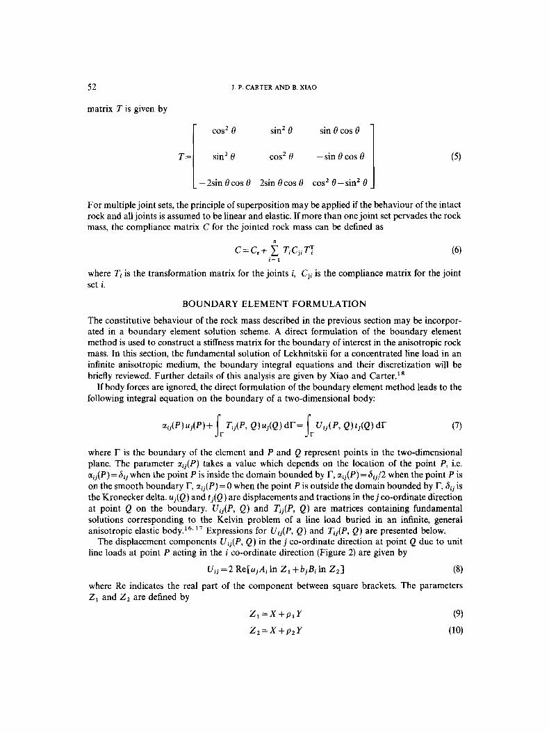
Some of the integrals in equation (22) can be written in the form

I = Jrk In ( X +pi Y ) N ; dT

If the point P is the same as the point Q, then both X and Y in equation (27) are identically zero and obviously the integrand becomes singular. Thus, care must be exercised if these integrals are to be evaluated accurately using numerical procedures.

When a node is located at a corner, a discontinuity in the nodal traction is likely to occur at that node, and this presents difficulties for the numerical analysis. Several schemes for dealing with this problem have been described by Brebbia and D o m i n g u e ~ . ~ ~ Their suggested use of discontinuous elements at the corner has been adopted in the boundary element scheme described in this paper.

Equation (22) can be written in matrix form for all the boundary points, so that

H U = G P (28) where H and G are matrices of influence coefficients, and vectors U and P contain the nodal displacements and tractions of the boundary points, respectively.

COUPLING OF FINITE AND BOUNDARY ELEMENTS

For the sake of completeness, a brief description of the procedure to couple finite and boundary element methods will be presented here.

Suppose that a body is divided into a finite element region Rf, and a boundary element region !& as shown in Figure 3. Define the displacement vectors as follows:

Uf =displacements in the region Rf Ufb = displacements on the interface between nf and fib approached from the region Rf Ufo =displacements in the region Of, excluding Ufb, i.e.

U f = [ U f O , UfblT (29) Ub =displacements in the region fib Ubf=displacements on the interface between Rf and f i b approached from the region fib UbO =displacements in the region fib, excluding U b f , i.e.

Ub=[Ubf, UbOIT (30)

I

I I

I , _ - - - .__-

I I - _ _ _ - - - - - - - - - - - Q f I

Figure 3. Coupled finite element and boundary element regions: (a) partially coupled mesh; (b) fully coupled mesh

56 J P. CARTER AND B. XIAO

Considering the compatibility conditions for displacement and the equilibirum of force on the interface leads to

Ufb = Ubf (31)

Ffb -k Fbf =o (32) In the region Rf, a finite element formulation has been adopted. In the usual manner the

principle of virtual work is used to obtain a set of linear stiffness equations, i.e.

K f U f = Ff (33) where Kf is the global stiffness matrix, CJ, is the nodal displacement vector and Ff is the nodal force vector.

In the region Rb, the boundary element formulation may be written as

H Ub= GPb (34) Equations (33) and (34) can be combined by treating the boundary element domain as an equivalent finite element. By inverting matrix G, equation (34) may be written as

G-'(HUb) = Pb (35) The tractions at the nodes can be converted into a vector of equivalent nodal forces of the same

type used in the finite element analysis. This is done by weighting the boundary tractions by the interpolation function used for the displacements, i.e.

F b = MPb (36) The global matrix M is assembled from the matrices Mk for each interface element, where Mk is given by

and

Nikj = irk Ni Nj dT (38)

where N i is the boundary element interpolation function and I is a unit matrix. If both sides of equation (35) are multiplied by the matrix M, i.e.

M(G- 'H) Ub = MPb = Fb (39)

K b Ub = Fb (40) where Kb= MG-'H. The stiffness matrix, Kb, and the load vector, Fb, for the boundary element region can be incorporated as 'super element' contributions in the global stiffness matrix and load vector used in the standard finite element procedure. Finally, it is noted that the stiffness matrix for the boundary element region is non-symmetric and, consequently, the global stiffness matrix

then equation (39) can be written as

COUPLED FINITE AND BOUNDARY ELEMENT FORMULATION 57

will also be non-symmetric. An efficient skyline solution technique for non-symmetric equations has been used to obtain the numerical results presented in this paper.

VERIFICATIONS OF COMPUTER CODE

In order to validate the present formulation, several example problems have been solved. Problems involving homogeneous compression, a tunnel excavated in an isotropic medium and normal pressure distributed uniformly over the surfaces of a cavity in an anisotropic medium have been studied. The choice of relatively coarse discretizations for both the finite element and boundary element regions was designed to examine how well the linked algorithm can predict the displacements and stress gradients. The results of the numerical analyses have been compared with analytical solutions.

Homogeneous compression

In this section the coupling procedure, for the case where the boundary and finite element regions are partially coupled, is validated for an isotropic material.

The simple problem of the compression of an initially stress-free, rectangular section under conditions of plane strain has been solved for two cases, i.e. one-dimensional compression

23 22 1 6 9 14 17 21 - - - - I-I-i

27 T 23 22 1 6 9 14 17

27

l 211 0 " 0 I-

l l 9

1

31 36 5 21

@)

Figure 4. Coupled finitie element and boundary element mesh 1 for homogeneous compression: (a) one-dimensional compression; (b) biaxial compression

58 J. P. CARTER AND B. XIAO

I 23 l t 39

17

24 + +

Y 27 7 35

t. L I

Figure 5. Coupled finitie element and boundary element mesh 2 for homogeneous compression: (a) one-dimensional compression; (b) biaxial compression

(Figures 4(a) and 5(a)) and biaxial compression (Figures 4(b) and 5(b)). The results have been presented in the form of

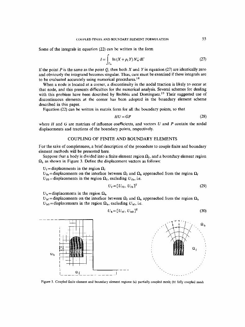
where t and t2 represent non-dimensional stiffness coefficients for one-dimensional cmpression and biaxial compression, respectively. G is the elastic shear modulus, v is Poisson’s ratio and L is the Lame modulus. 6 represents nodal displacement in the x and y directions for meshes 1 and 2, respectively (Figures 4 and 5). The values of these stiffness coefficients at selected points are compared with analytical results in Tables I and 11. Good agreement is evident.

Tunnel excavated in an isotropic medium

In this hypothetical example, the excavation of a circular tunnel in an isotropic medium is simulated. The circular interface between the finite element and boundary element regions has been located at 2.6 times the cavity radius, a, and the boundary element region is fully coupled to

COUPLED FINITE AND BOUNDARY ELEMENT FORMULATION 59

Table I. Comparison of coupled FE-BE and analytical solutions (mesh 1)

One-dimensional compression Biaxial compression

qL 5 - - ( l - v Z ) 2 - E S

qL 5 -~ '-(1+2G)S

Node Numerical

17 0.995 14 1.060 9 1.135 6 1.221 1 1.322

22 1.607 23 1.982

Analytical

1 ~OOO 1.066 1.143 1.230 1.333 1 - 6 0 24300

Numerical

0994 1.059 1-135 1.220 1.322 1 608 1.983

Analytical

1 Qoo 1.066 1.143 1.230 1.333 1.600 2900

Table 11. Comparison of coupled FE-BE and analytical solutions (mesh 2)

One-dimensional compression Biaxial compression

Node Numerical Analytical Numerical Analytical

23 2-01 8 2.000 2.008 2.000 24 2.745 2.667 2.689 2,667 25 4.032 4.000 3.960 4000

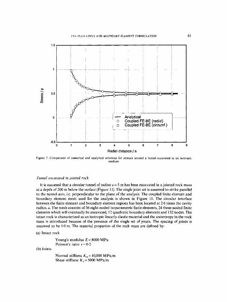
the finite element region. The numerical solutions were obtained using a mesh similar to that depicted in Figure 11, i.e. 36 eight-noded finite elements and 12 quadratic boundary elements. The in situ state of stress in the ground was idealized as uniaxial with zero vertical stress and a horizontal stress of magnitude, q. This is not meant to represent reality but merely to provide a check on complete coupling procedures. Poisson's ratio for the medium was assumed to be v = 0. The predicted radial and circumferential displacements and stress distributions along a ray at 45" to the horizontal x axis are shown in Figures 6 and 7. The results agree well with the analytical solutions (e.g. Reference 26).

Normal pressure distributed unijormly over the surface of a cavity in an anisotropic medium

The third example provides a check on the coupling procedure and the formulation for an anisotropic material. It involves a circular cavity in an infinite anisotropic medium to which an internal pressure ( p = 10 MPa) is applied. Initially the medium was assumed to be unstressed. The circular interface between the finite element and boundary element regions has been located at 2.6 times the cavity radius, a. As with the previous example, the numerical solutions were obtained using a mesh similar to that depicted in Figure 11, i.e. 36 finite elements and 12 boundary elements. The medium was assumed to consist of an intact rock with E = 8000 MPa, v = 0.2 and

60

Ex 1.637 -0.487 0.650

=(lop4) -0-487 2.137 0.217 [:lyy 1 0-650 0.217 4.250

J. P. CARTER AND B. XlAO

I:]

1

0.5

Y O c E" 8

E

e

m - 9 -0.5

X m h

-1

-1.5

-2

h U h u h h

U h h " " "

Radial distance / a

Figure 6. Comparison of numerical and analytical solutions for a tunnel excavated in an isotropic medium

a set of parallel joints defined by K , = 10,000 MPa/m, K , = 5000 MPa/m and S = 1.0 m, which are inclined at 30" to the x axis. The elastic compliance relations for this body may be written as

(43)

where the compliance components in equation (44) are in units of m2/MN, and the x axis is horizontal. Figure 8 shows the predicted radial and circumferential displacements around the surface of the cavity. The distributions of radial and circumferential displacements and stresses along a ray at 45" to the horizontal x axis are shown in Figures 9 and 10, respectively. The coupled numerical solutions agree well with the analytical solutions.

APPLICATIONS

To demonstrate the applicability of the present formulation to more realistic problems involving jointed rock masses, the analyses of a tunnel and a basement excavated in a regularly jointed rock mass are presented here.

COUPLED FINITE AND BOUNDARY ELEMENT FORMULATION 61

1.5

1

n v) 0.5 ?? El

- v)

0

-0.5

Analytical Coupled FE-BE (radial) Coupled FE-BE (circumf.)

0 1 2 3 4 5 6 7 a 9

Radial distance / a

Figure 7. Comparison of numerical and analytical solutions for stresses around a tunnel excavated in an isotropic medium

Tunnel excavated in jointed rock

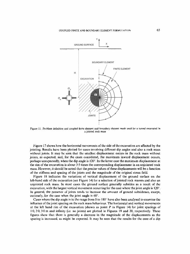
It is assumed that a circular tunnel of radius a = 5 m has been excavated in a jointed rock mass at a depth of 200 m below the surface (Figure 11). The single joint set is assumed to strike parallel to the tunnel axis, i.e. perpendicular to the plane of the analysis. The coupled finite element and boundary element mesh used for the analysis is shown in Figure 11. The circular interface between the finite element and boundary element regions has been located at 2.6 times the cavity radius, a. The mesh consists of 36 eight-noded isoparametric fintie elements, 24 three-noded finite elements which will eventually be excavated, 12 quadratic boundary elements and 132 nodes. The intact rock is characterized as an isotropic linearly elastic material and the anisotropy in the rock mass is introduced because of the presence of the single set of joints. The spacing of joints is assumed to be 1.0 m. The material properties of the rock mass are defined by:

(a) Intact rock

Young’s modulus E = 8000 MPa Poisson’s ratio v = 0 2

(b) Joints

Normal stiffness K , = 10,000 MPa/m Shear stiffness K , = 5000 MPa/m

62

20

15

10 h

E E v

v)

E c

5 2 - 2 a .u, 0 0

-5

-1c

J. P. CARTER AND B. XIAO

Coupled FE-BE (radial)

0 100 200 300 400

Angle 0 (degrees)

Figure 8. Comparison of numerical and analytical solutions for dispalcements around the boundary in an anisotropic medium

The in situ vertical stress (prior to tunnelling) is assumed to vary with depth according to

(T, = yH (44) where y is the unit weight of the rock and His the depth beneath the surface. The in situ horizontal stress is

o ~ = K o , + ~ (45) where 9 is the surface value of the horizontal stress. The unit weight of the rock mass is assumed as y=O*O25 MN/m3, the in situ stress coefficient K=2.0 and q is assumed equal to zero in this example. At a depth of 200 m the magnitudes of the vertical and horizontal stresses are 5 and 10 MPa, respectively. The average values are assumed to be approximately the same over the full depth interval of the tunnel.

The contours of the displacement components in the x co-ordinate direction for dip angles 0 and 30" are presented in Figures 12 and 13. It can be seen that there are significant differences in these patterns of displacement. In Figure 12, the contours of the displacement are symmetric about the horizontal axis and antisymmetric about the vertical co-oridnate axis, as expected for the case of a dip angle of 0". In contrast to this, the pattern in Figure 13 is not symmetric about the co-ordinate axes. As might be predicted, the presence of joints induces some anisotropy in the rock mass.

COUPLED FINITE AND BOUNDARY ELEMENT FORMULATION 63

1

1' h

E E v 4- c a,

E - 3 a v)

i i !

I

c, - Analytical o Coupled FE-BE (radial)

Coupled FE-BE (circumf.)

1 2 3 4 5 6 7 8 9

Radial distance / a

Figure 9. Comparison of numerical and analytical solutions for displacements along a ray at 45" to the horizontal axis in an anisotropic medium

Basement excavated in jointed rock

The problem considered here is a basement excavated in jointed rock to a depth of 25 m. Each joint within the single joint set is assumed to strike perpendicular to the plane of the analysis and conditions of plane strain have been adopted. The coupled mesh shown in Figure 14 consists of 120 finite elements (of which 50 elements will be excavated), 46 boundary elements and a total of 452 nodes. The elements to be 'excavated' are indicated by the shaded region in Figure 14. Note that a smooth, rigid, vertical boundary has been assumed at a horizontal location corresponding to x = 100 m, to allow an analysis of only one-half of the problem geometry. For isotropic rock masses and rock masses in which the joint sets are either horizontal or vertical, this will, in fact, be a plane of symmetry. It is not necessarily a plane of symmetry for more general cases of inclined rock joints. However, it has been found for these general cases that the results of the analyses in which the full excavation geometry has been discretized are not significantly different from those obtained from analyses with the mesh and boundary conditions shown in Figure 14.

In this problem, the intact rock was treated as a linearly elastic material characterized by Young's modulus E = 5000 MPa and Poisson's ratio v=O.25. The blocks of intact rock are separated by a regular set of parallel joints. All joints in the set have the same orientation and mechanical properties and their spacing S is constant. The elastic behaviour of each joint is characterized by a shear stiffness K , = 750 MPa/m and an uncoupled normal stiffness K , = 3000 MPa/m.

64 J. P. CARTER AND B. XIAO

1

0.5

0

-0.5

-1

Coupled FE-BE (radial) Coupled FE-BE (circumf.)

1 2 3 4 5 6 7 8

Radial distance / a

Figure 10. Comparison of numerical and analytical solutions for stresses along a ray at 45" to the horizontal axis in an anisotropic medium

It is assumed that immediately before any excavation the state of stress in the ground is such that the vertical and horizontal directions are principal stress directions. At any given depth, the magnitude of the stress is the same in all horizontal directions. The magnitude of the total vertical stress is given by

B, = yH (46) where y is the unit weight of the rock mass and H is the depth below the original ground surface. The unit weight of the rock mass is assumed as y =0.025 MN/m3 for this example. The total in situ horizontal stress (prior to excavation) is assumed to vary with the vertical stress according to

Bh = q + 20, (47) where q = O 3 MPa.

The deformed meshes for cases where the dip angles are 0 and 120" are presented in Figures 15 and 16. It may be seen that in both cases the stress release causes inward movements of the side of the excavation, downward settlement of the ground surface and upward heave of the base, as expected, but in each case the pattern of deformation is quite different. For example, the maximum horizontal movement for a dip angle of 120" is approximately three times that which occurs when the dip angle is 0". However, the maximum base heave for the case of 0" is about twice the maximum heave that occurs when the dip angle is 120".

COUPLED FINITE AND BOUNDARY ELEMENT FORMULATION 65

GROUND SURFACE

BOUNDARY ELEMENT

,/ FINITEELEMENT

H

Figure 11. Problem definition and coupled finite element and boundary element mesh used for a tunnel excavated in a jointed rock mass

Figure 17 shows how the horizontal movements of the side of the excavation are affected by the jointing. Results have been plotted for cases involving different dip angles and also a rock mass without joints. It may be seen that the smallest displacement occurs in the rock mass without joints, as expected, and, for the cases considered, the maximum inward displacement occurs, perhaps unexpectedly, when the dip angle is 120". In the latter case the maximum displacement at the rim of the excavation is about 3.5 times the corresponding displacement in an unjointed rock mass. However, it should be noted that the precise values of these displacements will be a function of the stiffness and spacing of the joints and the magnitude of the original stress field.

Figure 18 indicates the variations of vertical displacement of the ground surface on the left-hand side of the excavation (see Figure 14) for a selection of jointed rock masses and also an unjointed rock mass. In most cases the ground surface generally subsides as a result of the excavation, with the largest vertical movement occurring for the case where the joint angle is 120". In general, the presence of joints tends to increase the amount of ground subsidence, except, curiously, for the case when the joint angle is 60".

Cases where the dip angle is in the range from 0 to 180" have also been analysed to examine the influence of the joint spacing on the rock mass behaviour. The horizontal and vertical movements at the left hand rim of the excavation (shown as point P in Figure 14) for joint spacings of 1.0,2.0, 3.0 m and infinity (i.e. no joints) are plotted in Figures 19 and 20, respectively. These figures show that there is generally a decrease in the magnitude of the displacements as the spacing is increased, as might be expected. It may be seen that the results for the case of a dip

1 C u m u l a t i v e n o d a l v a r i a b l e 1 LEGEND

-1 343E-02

-0 9511-03

3

4 476E-03

111 rn 8.9511-03

1 3431-02

AFENA - A CIRCULAR TUNNEL EXCAVATED I N A JOINTED ROCK MASS

Figure 12. Contours of the displacement components in the x co-ordinate direction for a dip angle of 0"

1 C u m u l a t i v e n o d a l v a r i a b l e 1 LEGEND

-1 474E-02

0 -4.9311-03

9 7868-03

1 9698-02

AFENA - A CIRCULAR TUNNEL EXCAVATED I N A JOINTED ROCK MASS

Figure 13. Contours of the displacement components in the x co-ordinate direction for a dip angle of 30"

COUPLED FINITE AND BOUNDARY ELEMENT FORMULATION

Deflections magnified by 120

60.

50.

40. -

30.

140. 150. 160. 170. 180. 190. 11 00. AFENA - Basement excavation (Jointed rock masses, dip 0 degrees)

67

415 406 385 P 405

*1 E =5MxIMPa

uh I 20, + 0.5 MPa y =0.25MPa/m K, =750MPa/m K, = 3OOOMPa/m

v 50.25

21

452

4 A 421 447

I I I I I I I I I I I 0 10 20 30 40 50 60 70 80 90 100 (m)

Figure 14. Problem definition and coupled finite element and boundary element mesh used for a basement excavated in a jointed rock mass

Figure 15. Deformed mesh in the finite element region for a dip angle of 0"

68 J. P. CARTER AND B. XIAO

Deflections magnified by 120

60.

50.

40.

30.

140. 150. 160. 170. 180. 190. I1 00. AFENA - Basement excavation (Jointed rock masses, dip 120 degrees)

Figure 16. Deformed mesh in the finite element region for a dip angle of 120"

-0- No joints --.e=o" -e-6 = 30' - e = 60. -- e = 90"

-+ e = 150" + 8 = 120'

5 10 15

i 1

20 25 30

Horizontal displacement (mm)

Figure 17. Variations of horizontal displacements at the vertical excavation boundary

5

-20 -1 5 -10 -5 0

Distance from the vertical boundary of the cut (m)

Figure 18. Variations of vertical displacements at the ground surface

+ S = 2.0 m -- S = 3.0 m

- 0 50 100 150 200

Dip angle 8 (degrees)

Figure 19. Comparison of horizontal displacements at the top of the excavation

J. P. CARTER AND B. XIAO

5

a

-[

-1 I

-1,

-e- No joints - S = l . O m + S = 2.0 m -A- S = 3.0 m

U 50 100 150 200

Dip angle 0 (degrees)

Figure 20. Comparison of vertical displacements at the top of the excavation

angle of 0" are relatively insensitive to the joint spacing. However, at other dip angles the predictions are quite sensitive to joint spacing.

CONCLUSIONS

The purpose of the present study was to develop a coupled finite and boundary element formulation for the analysis of excavation in jointed rock. The near-field rock was discretized using the finite elements. The presence of joints in the near field has been included implicitly by treating the rock mass as an appropriate anisotropic elastic continuum. The far-field rock mass was also modelled as an anisotropic elastic continuum through a boundary element formulation, which is based on the fundamental solution of Lekhnitskii for a concentrated line load in an infinite anisotropic medium. Example problems have been solved to demonstrate the capability, accuracy and efficiency of the present formulation. Moreover, the results of a tunnel and a basement excavated in jointed rock show that the presence of joints induces anisotropy in the rock mass and the orientation and spacing of the joint sets have a considerable influence on the behaviour of a rock mass.

ACKNOWLEDGEMENTS

The work described in this paper forms part of an ongoing study into deep excavations in urban environments, which is supported by a grant from the Australian Research Council. Support

COUPLED FINITE AND BOUNDARY ELEMENT FORMULATION 71

for this work is also provided in the form of research scholarships awarded to the second author by the Australian Development Cooperation Scholarship Scheme and by the Centre for Geotechnical Research at the University of Sydney.

1 .

2.

3.

4.

5.

6.

7.

8.

9.

10.

11.

12.

13.

14. 15.

16.

17. 18.

19.

20.

21.

22.

23.

24.

REFERENCES

0. C. Zienkiewicz, D. W. Kelly and P. Bettess, ‘The coupling of the finite element method and boundary solution methods’, Int. j. numer. methods eng., 11, 335-375 (1977). C. A. Brebbia and P. Georgiou, ‘Combination of boundary and finite elements in elastostatics’, Appl. Math. Modetling,

G. Beer and J. L. Meek, ‘Coupled finite element-boundary element analysis of infinite domain problems in geomechanics’, in E. Hinton, P. Bettess and R. W. Lewis (eds), Numerical Methodsfor Coupled Problems, Pineridge Press, Swansea, 1981, pp. 605-629. B. H. G. Brady and A. Wassyng, ‘A coupled finite element-boundary element method of stress analysis’, Int. J. Rock Mech. Min. Sci. Geomech. Abstr., 23, 475485 (1981). D. Yeung and B. H. G. Brady, ‘A hybrid quadratic isoparametric finiteboundary element code for underground excavation analysis, Proc. 23rd U.S. Symposium on Rock Mechanics, University of California, Berkeley, 1982, Chapter 72, pp. 692-703. G. Beer, ‘Finite element, boundary element and coupled analysis of unbounded problems in elastostatics’, Int. j . numer. methods eng., 19, 567-580 (1983). G. Beer, ‘Implementation of combined boundary element-finite element analysis with applications in geomechanics’, in P. K. Banerjee and J. 0. Watson (eds), Developments in Boundary Element Methods+, Elsevier, London, 1986,

T. Ohkami, Y. Mitsui and T. Kusama, ‘Coupled boundary element/finite element analysis in geomechanics including body forces’, Comput. Geotech., 1, 263-278 (1985). A. Varadarajan, K. G. Sharma and R. B. Singh, ‘Some aspects of coupled FEBEM analysis of underground openings’, Int. j. numer. anal. methods geomech., 9, 557-571 (1985). A. Varadarajan, K. G. Sharma and R. B. Singh, ‘Elasto-plastic analysis of an underground opening by FEM and coupled FEBEM’, Int. j. numer. anal. methods geomech., 11, 475487 (1987). G. Swoboda, W. Mertz and G. Beer, ‘Rheological analysis of tunnel excavations by means of coupled finite element (FEMtboundary element (BEM) analysis’, Int. j. numer. anal. methods geomech., 11, 115-129 (1987). G. Swoboda, W. Mertz and A. Schmid, ‘Three dimensional numerical models to simulate tunnel excavation’, in S. Pietruszczak and G. N. Pande (eds), Numerical Models in Geomechanics NUMOG Ill, Elsevier, London 1989, pp. 536548. L. J. Lorig, B. H. G. Brady and P. A. Cundall, ‘Hybrid distinct element-boundary element analysis of jointed rock’, Int. J. Rock Mech. Min. Sci. Geomech. Abstr., 23, 303-312 (1986). A. E. Green, ‘A note on stress systems in aeolotropic materials’, Philos. Mag., 34,41&418 (1943). F. J. Rizzo and D. J. Shippy, ‘A method for stress determination in plane anisotropic elastic bodies’, J. Composite Mater., 4, 3 U (1970). S. G. Lekhnitskii, ‘Plane static problem of the theory of elasticity of an anisotropic body’, Prikl. Mat . I. Mech., 1, (1937). S . G. Lekhnitskii, Theory of Elasticity of an Anisotropic Body, Mir., Moscow, 1981. B. Xiao and J. P. Carter, ‘Boundary element analysis of anisotropic rock masses’, Research Report No . R657, School of Civil and Mining Engineering, University of Sydney, 1992. J. M. Duncan and R. E. Goodman, ‘Finite element analysis of slopes in jointed rocks’, Contract Report No. 568-3, U.S. AEWES, Corps of Engineers, Vickaburg, Mississippi, 1968. L. Wardle and C. Gerrard, ‘The equivalent anisotropic properties of layered rock and soil masses’, Rock Mechanics, 4,

B. Amadei and R. E. Goodman, ‘A 3-D constitutive relation for fractured rock mass’, Proc. Int. Symp. on the Mechanical Behaviour of Structured Media, Part B, Ottawa, 1981, pp. 249-268. J. P. Carter and H. Alehlossein, ‘Analysis of tunnel distortion due to an open excavation in jointed rock‘, Comput. Geotech., 9, 209-231 (1990). J. J. Liao and B. Amadei, ‘Surface loading of anisotropic rock masses’, J. geotech. eng. dir. ASCE, 17, 1779-1800 (1991).

3, 212-220 (1979).

pp. 191-225.

155-175.

H. W. Turnbull, Theory of Equations, Interscience Publishers Inc. Oliver and Boyd, Edinburgh London, 1946. 25. C. A. Brebbia and J. Dominguez, Boundury Elements-An Introductory Course, Computational Mechanics Publica-

tions, Southampton, 1981, 292 p. 26. M. J. Pender, ‘Elastic solutions for a deep circular tunnel’, Geotechnique, 30, 216-222 (1980).