9.13 Fixed Earth-Support Method for Penetration into...

9.13 Fixed Earth-Support Method for Penetration into Sandy Soil

When using the fixed earth support method, we assume that the toe of the pile is restrainedfrom rotating, as shown in Figure 9.28a. In the fixed earth support solution, a simplifiedmethod called the equivalent beam solution is generally used to calculate L3 and, thus, D.The development of the equivalent beam method is generally attributed to Blum (1931).

In order to understand this method, compare the sheet pile to a loaded cantilever beamRSTU, as shown in Figure 9.29. Note that the support at T for the beam is equivalent to theanchor load reaction (F) on the sheet pile (Figure 9.28). It can be seen that the point S of thebeam RSTU is the inflection point of the elastic line of the beam, which is equivalent to pointI in Figure 9.28. It the beam is cut at S and a free support (reaction Ps) is provided at thatpoint, the bending moment diagram for portion STU of the beam will remain unchanged.This beam STU will be equivalent to the section STU of the beam RSTU. The force P� shownin Figure 9.28a at I will be equivalent to the reaction Ps on the beam (Figure 9.29).

The following is an approximate procedure for the design of an anchored sheet-pilewall (Cornfield, 1975). Refer to Figure 9.28.

Step 1. Determine L5, which is a function of the soil friction angle �� below thedredge line, from the following:

476 Chapter 9: Sheet Pile Walls

FIGURE 9.28 Fixed earth support method for penetration of sandy soil

(a) Pressure diagram

Sand

γ, φ′

γsatφ′

SandAnchorWater table

Deflectedshape ofsheet pile

B G

E

I

A

C

F

z

J

D

D

P′

O′

��2

��1

L3

L5

L2

l2

l1L1

L5

F

H

(b) Moment diagram

�� (deg)

30 0.0835 0.0340 0

L 5

L1 1 L2

Step 2. Calculate the span of the equivalent beam as l2 � L2 � L5 � L�.Step 3. Calculate the total load of the span, W. This is the area of the pressure

diagram between O� and I.Step 4. Calculate the maximum moment, Mmax, as WL�/8.Step 5. Calculate P� by taking the moment about O�, or

(9.82)

Step 6. Calculate D as

(9.83)

Step 7. Calculate the anchor force per unit length, F, by taking the moment about I, or

(moment of area ACDJI about I)

Example 9.9

Consider the anchored sheet-pile structure described in Example 9.5. Using the equiva-lent beam method described in Section 9.13, determine

a. Maximum momentb. Theoretical depth of penetrationc. Anchor force per unit length of the structure

Solution

Part aDetermination of L5: For �� 30°,

L5

L1 1 L25 0.08

F 51

Lr

D 5 L5 1 1.2Å

6Pr(Kp 2 Ka)gr

Pr 51

Lr (moment of area ACDJI about O r)

9.13 Fixed Earth-Support Method for Penetration into Sandy Soil 477

Figure 9.29 Equivalent cantilever beam concept

Moment diagram

Beam

UTR S

Ps

L5 � 0.73

Net Pressure Diagram: From Example 9.5, , Kp � 3, � � 16 kN/m3, �� 9.69

kN/m3, �1� � 16.27 kN/m2, �2� � 35.97 kN/m2. The net active pressure at a depth L5

below the dredge line can be calculated as

�2� � ��(Kp � Ka)L5 � 35.97 � (9.69)(3 � 0.333)(0.73) � 17.1 kN/m2

The net pressure diagram from z � 0 to z � L1 � L2 � L5 is shown in Figure 9.30.

Maximum Moment:

� 197.2 kN/m

L� � l2 � L2 � L5 � 1.52 � 6.1 � 0.73 � 8.35 m

Part b

(moment of area ACDJI about O�)Pr 51

Lr

Mmax 5WLr

85

(197.2) (8.35)

85 205.8 kN ? m>m

1 a1

2b (0.73) (35.97 1 17.1)

W 5 a1

2b (8.16 1 16.27) (1.52) 1 a

1

2b (6.1) (16.27 1 35.97)

Ka 5 13

L5

3.05 1 6.15 0.08


17.1 kN/m2

35.97 kN/m2

1.53 m = l1

6.1 m = L2

C

F

D

JI

A

O′

P′L5 = 0.73 m

l2 = 1.52 m 16.27 kN/m2

8.16 kN/m2

FIGURE 9.30

-

� 114.48 kN/m

From Eq. (9.83)

Part cTaking the moment about I (Figure 9.30)

� 88.95 kN/m ■

9.14 Field Observations for Anchor Sheet Pile Walls

In the preceding sections, large factors of safety were used for the depth of penetration, D.In most cases, designers use smaller magnitudes of soil friction angle, ��, thereby ensur-ing a built-in factor of safety for the active earth pressure. This procedure is followed pri-marily because of the uncertainties involved in predicting the actual earth pressure towhich a sheet-pile wall in the field will be subjected. In addition, Casagrande (1973)observed that, if the soil behind the sheet-pile wall has grain sizes that are predominantlysmaller than those of coarse sand, the active earth pressure after construction sometimesincreases to an at-rest earth-pressure condition. Such an increase causes a large increase inthe anchor force, F. The following two case histories are given by Casagrande (1973).

Bulkhead of Pier C—Long Beach Harbor, California (1949)

A typical cross section of the Pier C bulkhead of the Long Beach harbor is shown in Figure9.31. Except for a rockfill dike constructed with 76 mm (3 in.) maximum-size quarrywastes, the backfill of the sheet-pile wall consisted of fine sand. Figure 9.32 shows the

c

Approximate

F 51

8.35 Ea

1

2(16.27) (3.05) a0.73 1 6.1 1

3.05

3b 1 (16.27) (6.1) a0.73 1

6.1

2b

1 a1

2b (6.1) (35.97 2 16.27) a0.73 1

6.1

3b 1 a

1

2b (35.97 1 17.1) (0.73) a

0.73

2b

U

D 5 L5 1 1.2 Å

6Pr(Kp 2 Ka)gr

5 0.73 1 1.2 Å

(6) (114.48)

(3 2 0.333) (9.69)5 6.92 m

cApproximate

P9 51

8.35 H

£1

2≥(16.27) (3.05)£2

33 3.05 2 1.53≥ 1 (16.27) (6.1)£1.52 1

6.1

2≥

1 £1

2≥(6.1) (35.97 2 16.27)£1.52 1

2

33 6.1≥ 1 £1

2≥(35.97 1 17.1)

3 (0.73)£1.52 1 6.1 10.73

2≥

X

9.14 Field Observations for Anchor Sheet Pile Walls 479


variation of the lateral earth pressure between May 24, 1949 (the day construction wascompleted) and August 6, 1949. On May 24, the lateral earth pressure reached an activestate, as shown in Figure 9.32a, due to the wall yielding. Between May 24 and June 3, theanchor resisted further yielding and the lateral earth pressure increased to the at-rest state(Figure 9.32b). However, the flexibility of the sheet piles ultimately resulted in a gradualdecrease in the lateral earth-pressure distribution on the sheet piles (see Figure 9.32c).

Figure 9.31 Pier C bulkhead—Long Beach harbor (Adapted after Casagrande, 1973)

Figure 9.32 Measured stresses at Station 27 � 30—Pier C bulkhead, Long Beach (Adapted afterCasagrande, 1973)

+5.18 m

+1.22 m

10 m

Scale

0

–18.29 m

–11.56 m

–3.05 m

1V: 0.58H

Fine sandhydraulic fill

Tie rod–76 mm dia.

1V: 1.5 H

El.0Mean low water level

MZ 38 Steel sheet pile

Fine sand

Rock dike76 mm maximumsize

May 24

(a) (b) (c)

+5.18 m +5.18 m +5.18 m

–3.05 m

–11.56 m

0 100 200 kN/m2

–11.56 m

Pressure scale

–11.56 m

–3.05 m –3.05 m

151.11MN/m2

177.33MN/m2

213.9MN/m2

June 3 August 6

9.14 Field Observations for Anchor Sheet Pile Walls 481

With time, the stress on the tie rods for the anchor increased as shown in the fol-lowing table.

Stress on anchor Date tie rod (MN/m2)

May 24, 1949 151.11June 3, 1949 177.33June 11, 1949 193.2July 12, 1949 203.55August 6, 1949 213.9

These observations show that the magnitude of the active earth pressure may vary withtime and depend greatly on the flexibility of the sheet piles. Also, the actual variations inthe lateral earth-pressure diagram may not be identical to those used for design.

Bulkhead—Toledo, Ohio (1961)

A typical cross section of a Toledo bulkhead completed in 1961 is shown in Figure 9.33.The foundation soil was primarily fine to medium sand, but the dredge line did cut intohighly overconsolidated clay. Figure 9.33 also shows the actual measured values of bend-ing moment along the sheet-pile wall. Casagrande (1973) used the Rankine active earth-pressure distribution to calculate the maximum bending moment according to the freeearth support method with and without Rowe’s moment reduction.

Maximum predicted Design method bending moment, Mmax

Free earth support method 146.5 kN-mFree earth support method with Rowe’s moment reduction 78.6 kN-m

14Depth (m)

205 kN-m

180 kN-m

81 kN-m

65 kN-mMay 1961

0 100 200kN-m

Scale

Dredgeline

0Top of fill

Tierod

2

4

6

8

10

12

Figure 9.33 Bendingmoment from strain-gage measurements attest location 3, Toledobulkhead (Adapted afterCasagrande, 1973)


Comparisons of these magnitudes of Mmax with those actually observed show that the field val-ues are substantially larger. The reason probably is that the backfill was primarily fine sandand the measured active earth-pressure distribution was larger than that predicted theoretically.

9.15 Free Earth Support Method for Penetration of Clay

Figure 9.34 shows an anchored sheet-pile wall penetrating a clay soil and with a granularsoil backfill. The diagram of pressure distribution above the dredge line is similar to thatshown in Figure 9.12. From Eq. (9.42), the net pressure distribution below the dredge line(from to ) is

For static equilibrium, the sum of the forces in the horizontal direction is

(9.84)

where

of the pressure diagram ACDforce per unit length of the sheet pile wall F 5 anchor

P1 5 area

P1 2 s6D 5 F

s6 5 4c 2 (gL1 1 grL2)

z 5 L1 1 L2 1 Dz 5 L1 1 L2

��2Dredge line

z

BF

E

�6

P1

z1

��1 C

A

D

Water level

O�L1

L2

D

Sand�sat, ��

Sand, �, ��

�sat� = 0c

ClayClay

F

l1

l2

Figure 9.34 Anchored sheet-pile wall penetrating clay

9.15 Free Earth Support Method for Penetration of Clay 483

Again, taking the moment about produces

Simplification yields

(9.85)

Equation (9.85) gives the theoretical depth of penetration, D.As in Section 9.9, the maximum moment in this case occurs at a depth

The depth of zero shear (and thus the maximum moment) may bedetermined from Eq. (9.69).

A moment reduction technique similar to that in Section 9.11 for anchored sheetpiles penetrating into clay has also been developed by Rowe (1952, 1957). This techniqueis presented in Figure 9.35, in which the following notation is used:

1. The stability number is

(9.86)

where cohesion .For the definition of and see Figure 9.34.

2. The nondimensional wall height is

(9.87)

3. The flexibility number is [see Eq. (9.74)]4.

The procedure for moment reduction, using Figure 9.35, is as follows:

Step 1. Obtain Step 2. Determine Step 3. Determine [from Eq. (9.86)].Step 4. For the magnitudes of and obtained in Steps 2 and 3, determine

for various values of from Figure 9.35, and plot against

Step 5. Follow Steps 1 through 9 as outlined for the case of moment reduction ofsheet-pile walls penetrating granular soil. (See Section 9.11.)

log r.

Md>Mmaxlog rMd>Mmax

SnaSn

a 5 (L1 1 L2)>Hr.Hr 5 L1 1 L2 1 Dactual .

Mmax 5 maximum theoretical moment

Md 5 design moment

r

a 5L1 1 L2

L1 1 L2 1 Dactual

L2 ,g, gr, L1 ,

(f 5 0)c 5 undrained

Sn 5 1.25c

(gL1 1 grL2)

L1 , z , L1 1 L2 .

s6D2 1 2s6D(L1 1 L2 2 l1) 2 2P1(L1 1 L2 2 l1 2 z1) 5 0

P1(L1 1 L2 2 l1 2 z1) 2 s6D¢ l2 1 L2 1D

2≤ 5 0

Or


Figure 9.35 Plot of against stability number for sheet-pilewall penetrating clay (From Rowe, P. W. (1957).“Sheet Pile Walls in Clay,”Proceedings, Institute of CivilEngineers, Vol. 7, pp. 654–692.)

Md>Mmax

0.60.7

� = 0.8

Log � = –2.0

Stability number, Sn

00.4

0.6

0.8Md

Mmax

1.0

0.5 1.0 1.5 1.75

0.60.7

� = 0.8

Log � = –2.6

0.4

0.6

0.8Md

Mmax

1.0

0.6

0.7

� = 0.8

Log � = –3.1

0.4

0.6

0.8Md

Mmax

1.0

Example 9.10

In Figure 9.34, let and Also, let and

a. Determine the theoretical depth of embedment of the sheet-pile wall.b. Calculate the anchor force per unit length of the wall.

Solution

Part aWe have

Ka 5 tan2¢45 2fr2≤ 5 tan2¢45 2

35

2≤ 5 0.271

c 5 41 kN>m2.fr 5 35°,gsat 5 20 kN>m3,g 5 17 kN>m3,l1 5 1.5 m.L1 5 3 m, L2 5 6 m,

9.15 Free Earth Support Method for Penetration of Clay 485

Figure 9.36 Free earthsupport method, sheet pilepenetrating into clay

and

From the pressure diagram in Figure 9.36,

and

From Eq. (9.85),

So,

2 (2) (153.36) (3 1 6 2 1.5 2 3.2) 5 0

(51.86)D2 1 (2) (51.86) (D) (3 1 6 2 1.5)

1 (20 2 9.81) (6) 4 5 51.86 kN>m2

s6 5 4c 2 (gL1 1 grL2) 5 (4) (41) 2 3(17) (3)

s6D2 1 2s6D(L1 1 L2 2 l1) 2 2P1(L1 1 L2 2 l1 2 z1) 5 0

z1 5

(20.73) ¢6 13

3≤ 1 (82.92) ¢6

2≤ 1 (49.71) ¢6

3≤

153.365 3.2 m

5 20.73 1 82.92 1 49.71 5 153.36 kN>m

P1 5 areas 1 1 2 1 3 5 1>2(3) (13.82) 1 (13.82) (6) 1 1>2(30.39 2 13.82) (6)

sr2 5 (gL1 1 grL2)Ka 5 3(17) (3) 1 (20 2 9.81) (6) 4 (0.271) 5 30.39 kN>m2

sr1 5 gL1Ka 5 (17) (3) (0.271) 5 13.82 kN>m2

Kp 5 tan2¢45 1fr2≤ 5 tan2¢45 1

35

2≤ 5 3.69

L1 � 3 m

L2 � 6 m

l1 � 1.5 m

l2 � 1.5 m

1.6 m � D

��1 � 13.82 kN/m2

��2 � 30.39 kN/m2

�6 � 51.86 kN/m2

1

2

3


or

Hence,

Part bFrom Eq. (9.84),

■

9.16 Anchors

Sections 9.9 through 9.15 gave an analysis of anchored sheet-pile walls and discussed howto obtain the force F per unit length of the sheet-pile wall that has to be sustained by theanchors. The current section covers in more detail the various types of anchor generally usedand the procedures for evaluating their ultimate holding capacities.

The general types of anchor used in sheet-pile walls are as follows:

1. Anchor plates and beams (deadman)2. Tie backs3. Vertical anchor piles4. Anchor beams supported by batter (compression and tension) piles

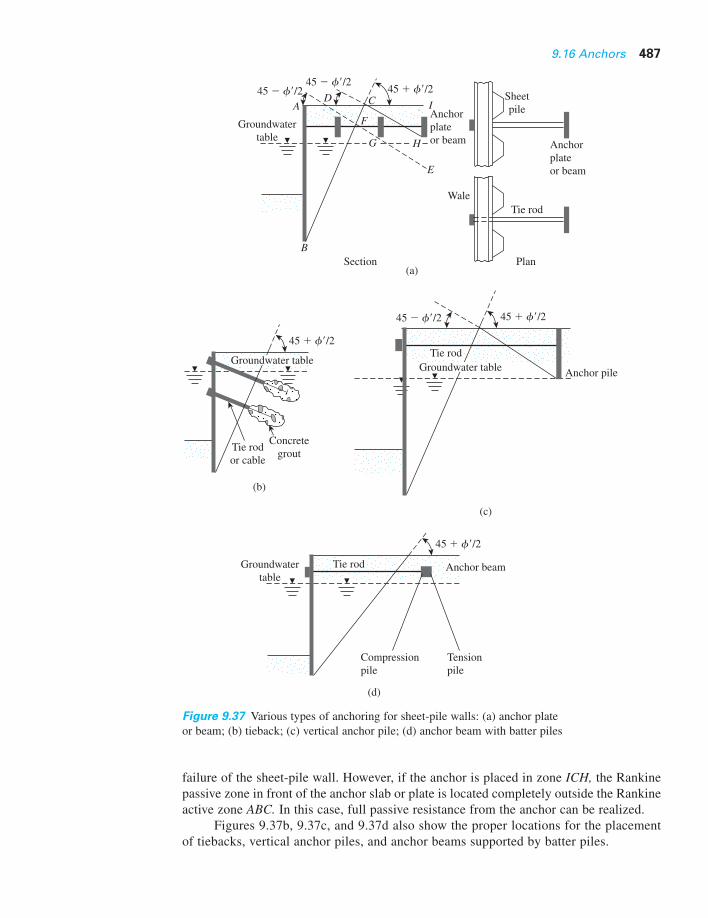
Anchor plates and beams are generally made of cast concrete blocks. (See Figure9.37a.) The anchors are attached to the sheet pile by tie-rods. A wale is placed at the frontor back face of a sheet pile for the purpose of conveniently attaching the tie-rod to thewall. To protect the tie rod from corrosion, it is generally coated with paint or asphalticmaterials.

In the construction of tiebacks, bars or cables are placed in predrilled holes (seeFigure 9.37b) with concrete grout (cables are commonly high-strength, prestressed steeltendons). Figures 9.37c and 9.37d show a vertical anchor pile and an anchor beam withbatter piles.

Placement of Anchors

The resistance offered by anchor plates and beams is derived primarily from the passiveforce of the soil located in front of them. Figure 9.37a, in which AB is the sheet-pile wall,shows the best location for maximum efficiency of an anchor plate. If the anchor is placedinside wedge ABC, which is the Rankine active zone, it would not provide any resistanceto failure. Alternatively, the anchor could be placed in zone CFEH. Note that line DFG isthe slip line for the Rankine passive pressure. If part of the passive wedge is located insidethe active wedge ABC, full passive resistance of the anchor cannot be realized upon

F 5 P1 2 s6D 5 153.36 2 (51.86) (1.6) 5 70.38 kN,m

D < 1.6 m

D2 1 15D 2 25.43 5 0

9.16 Anchors 487

Tensionpile

45 � ��/2

Compressionpile

Groundwatertable

Tie rod Anchor beam

(d)

(b)

45 � ��/2

Concretegrout

Tie rodor cable

Groundwater table

(a)

45 � ��/245 � ��/2

45 � ��/2

G

CDA

BSection Plan

H

E

WaleTie rod

SheetpileI

FAnchor plateor beam Anchor

plateor beam

Groundwatertable

45 � ��/245 � ��/2

Tie rod

Anchor pile

(c)

Groundwater table

Figure 9.37 Various types of anchoring for sheet-pile walls: (a) anchor plate or beam; (b) tieback; (c) vertical anchor pile; (d) anchor beam with batter piles

failure of the sheet-pile wall. However, if the anchor is placed in zone ICH, the Rankinepassive zone in front of the anchor slab or plate is located completely outside the Rankineactive zone ABC. In this case, full passive resistance from the anchor can be realized.

Figures 9.37b, 9.37c, and 9.37d also show the proper locations for the placementof tiebacks, vertical anchor piles, and anchor beams supported by batter piles.


9.17 Holding Capacity of Anchor Plates in Sand

Semi-Empirical Method

Ovesen and Stromann (1972) proposed a semi-empirical method for determining the ultimateresistance of anchors in sand. Their calculations, made in three steps, are carried out as follows:

Step 1. Basic Case. Determine the depth of embedment, H. Assume that the anchorslab has height H and is continuous (i.e., of anchor slab per-pendicular to the cross ), as shown in Figure 9.38, in which thefollowing notation is used:

Also,

(9.88)

where

active pressure coefficient with (see Figure 9.39a)

pressure coefficient

To obtain first calculate

(9.89)Kp sin dr 5W 1 Pa sin fr

12gH2

5W 1 1

2gH2Ka sin fr12gH2

Kp cos dr,

Kp 5 passive

dr 5 fr Ka 5

5 12 gH2(Kp cos dr 2 Ka cos fr)

Prult 5 12 gH2Kp cos dr 2 Pa cos fr 5 1

2 gH2Kp cos dr 2 12 gH2Ka cos fr

W 5 effective weight per unit length of anchor slab Prult 5 ultimate resistance per unit length of anchor

dr 5 friction angle between anchor slab and soil fr 5 effective soil friction angle Pa 5 active force per unit length of anchor Pp 5 passive force per unit length of anchor

section 5 `B 5 length

H

45 � ��/2

Pp

Pa

Sand

P�ult

45 � ��/2

��

��

��

Figure 9.38 Basic case: continuous vertical anchor in granular soil

9.17 Holding Capacity of Anchor Plates in Sand 489

Then use the magnitude of obtained from Eq. (9.89) to estimatethe magnitude of from the plots given in Figure 9.39b.

Step 2. Strip Case. Determine the actual height h of the anchor to be constructed. Ifa continuous anchor (i.e., an anchor for which ) of height h is placedin the soil so that its depth of embedment is H, as shown in Figure 9.40, theultimate resistance per unit length is

B 5 `

Kp cos drKp sin dr

30

35

40

45

Kp sin ��

�� = 25

Kp

cos

��

02

10

8

6

4

3

12

14

1 2 3

(b)

4 5

Arc of log spiral

Pa

Soil friction angle, ��(deg)

��

Ka

100.1

0.6

0.5

0.4

0.3

0.2

0.7

20 30

(a)

40 45

Figure 9.39 (a) Variation of for (b) variation of with (Based on Ovesen and Stromann, 1972)Kp sin dr

Kp cos drdr 5 fr,Ka


(9.90)

where

resistance for the strip casefor dense sand and 14 for loose sand

Step 3. Actual Case. In practice, the anchor plates are placed in a row with center-to-center spacing as shown in Figure 9.41a. The ultimate resistance ofeach anchor is

Sr,

Cov 5 19 Prus 5 ultimate

Prus 5 C Cov 1 1

Cov 1 ¢H

h≤S

Prult

c

Eq. 9.88

H

Sand

h P�us

��

Figure 9.40 Strip case: vertical anchor

��

Dense sand

Sand

Loose sand

(S� – B)/(H – h)

h

HB

S� S�

(Be

– B

)/(H

+ h

)

(b)

(a)

00

0.3

0.2

0.1

0.4

0.5

0.5 1.0 1.25

Figure 9.41 (a) Actualcase for row of anchors;(b) variation of

with

(Based on Ovesen andStromann, 1972)

(Sr 2 B)> (H 1 h)

(H 1 h)(Be 2 B)>


(9.91)

where length.

The equivalent length is a function of B, H, and h. Figure 9.41b shows aplot of against for the cases ofloose and dense sand. With known values of B, H, and h, the value of can be calculated and used in Eq. (9.91) to obtain

Stress Characteristic Solution

Neely, Stuart, and Graham (1973) proposed a stress characteristic solution for anchor pull-out resistance using the equivalent free surface concept. Figure 9.42 shows the assumedfailure surface for a strip anchor. In this figure, OX is the equivalent free surface. The shearstress (so) mobilized along OX can be given as

(9.92)

where

m � shear stress mobilization factor�o� � effective normal stress along OX

Using this analysis, the ultimate resistance (Pult) of an anchor (length � B andheight � h) can be given as

Pult � M�q (�h2)BFs (9.93)

where

M�q � force coefficientFs � shape factor� � effective unit weight of soil

The variations of M�q for m � 0 and 1 are shown in Figure 9.43. For conservativedesign, M�q with m � 0 may be used. The shape factor (Fs) determined experimentally isshown in Figure 9.44 as a function of B/h and H/h.

m 5so

so9 tan f9

Pult .BeSr,

(Sr 2 B)> (H 1 h)(Be 2 B)> (H 1 h)

Sr,

Be 5 equivalent

Pult 5 PrusBe

Figure 9.42 Assumed failure surface in soil forstress characteristic solution

H

h

O

X

m =

Pult

so

so��o tan ��

�

��

��o


m = 0m = 1

01

2

5

10

�� = 30°

�� = 40°

��= 45°20

M�

q (l

og s

cale

)50

100

200

1 2 3H / h

4 5

�� = 35°

Figure 9.43 Variation of M�q withH/h and �� (After Neeley et al., 1973.With permission from ASCE.)

Figure 9.44 Variation of shape factor withH/h and B/h (After Neeley et al., 1973. Withpermission from ASCE.)

2.0

B/h = 1.0

01 2 3

H / h

4 5

0.5

1.0

1.5

Shap

e fa

ctor

, Fs

2.0

2.5

2.75

3.5

5.0

Empirical Correlation Based on Model Tests

Ghaly (1997) used the results of 104 laboratory tests, 15 centrifugal model tests, and 9field tests to propose an empirical correlation for the ultimate resistance of single anchors.The correlation can be written as

(9.94)

where .A 5 area of the anchor 5 Bh

Pult 55.4

tan fr¢H2

A≤ 0.28

gAH


Ghaly also used the model test results of Das and Seeley (1975) to develop aload–displacement relationship for single anchors. The relationship can be given as

(9.95)

where displacement of the anchor at a load level P.Equations (9.94) and (9.95) apply to single anchors (i.e., anchors for which ).

For all practical purposes, when the anchors behave as single anchors.

Factor of Safety for Anchor Plates

The allowable resistance per anchor plate may be given as

where of safety.Generally, a factor of safety of 2 is suggested when the method of Ovesen and

Stromann is used. A factor of safety of 3 is suggested for calculated by Eq. (9.94).

Spacing of Anchor Plates

The center-to-center spacing of anchors, may be obtained from

where per unit length of the sheet pile.

Example 9.11

Refer to Figure 9.41a. Given: B � h � 0.4 m, S� � 1.2 m, H � 1 m, � � 16.51 kN/m3,and �� 35°. Determine the ultimate resistance for each anchor plate. The anchorplates are made of concrete and have thicknesses of 0.15 m.

Solution

From Figure 9.39a for �� 35°, the magnitude of Ka is about 0.26.

W � Ht�concrete � (1 m)(0.15 m)(23.5 kN/m3)

� 3.525 kN/m

From Eq. (9.89),

53.525 1 (0.5) (16.51) (1)2(0.26) (sin 35)

(0.5) (16.51) (1)25 0.576

Kp sin d9 5W 1 1>2gH2Ka sin f9

1>2gH2

F 5 force

Sr 5Pall

F

Sr,

Pult

FS 5 factor

Pall 5Pult

FS

Sr>B < 2

Sr>B 5 `u 5 horizontal

P

Pult5 2.2¢ u

H≤ 0.3

From Figure 9.39b with �� 35° and Kp sin �� 0.576, the value of Kp cos �� isabout 4.5. Now, using Eq. (9.88),

Pult� � �H2(Kp cos �� Ka cos ��)

� ( )(16.51)(1)2[4.5 � (0.26)(cos 35)] � 35.39 kN/m

In order to calculate Pus�, let us assume the sand to be loose. So, Cov in Eq. (9.90) isequal to 14. Hence,

For (S� � B)/(H � h) � 0.571 and loose sand, Figure 9.41b yields

So

Be � (0.229)(H � h) � B � (0.229)(1 � 0.4) � 0.4

� 0.72

Hence, from Eq. (9.91)

Pult � Pus� Be � (32.17)(0.72) � 23.16 kN ■

Example 9.12

Refer to a single anchor given in Example 9.11 using the stress characteristic solution.Estimate the ultimate anchor resistance. Use m � 0 in Figure 9.43.

Solution

Given: B � h � 0.4 m and H � 1 m.Thus,

B

h5

0.4 m

0.4 m5 1

H

h5

1 m

0.4 m5 2.5

Be 2 B

H 2 h5 0.229

Sr 2 B

H 1 h5

1.2 2 0.4

1 1 0.45

0.8

1.45 0.571

Prus 5 D C ov 1 1

C ov 1 aH

hb

T Prult 5 D 14 1 1

14 1 a1

0.4b

T 5 32.17 kN>m

12

12


From Eq. (9.93),

Pult � M�q�h2 BFs

From Figure 9.43, with �� 35° and H/h � 2.5, M�q � 18.2. Also, from Figure 9.44,with H/h � 2.5 and B/h � 1, Fs � 1.8. Hence,

Pult � (18.2)(16.51)(0.4)2(0.4)(1.8) � 34.62 kN ■

Example 9.13

Solve Example Problem 9.12 using Eq. (9.94).

Solution

From Eq. (9.94),

H � 1 m

A � Bh � (0.4 0.4) � 0.16 m2

■P ult 55.4

tan 35c(1)2

0.16d

0.28

(16.51) (0.16) (1) < 34.03 kN

P ult 55.4

tan f9a

H2

Ab

0.28

gAH

9.19 Ultimate Resistance of Tiebacks 495

9.18 Holding Capacity of Anchor Plates in Clay ( Condition)

Relatively few studies have been conducted on the ultimate resistance of anchor plates inclayey soils ( ). Mackenzie (1955) and Tschebotarioff (1973) identified the nature ofvariation of the ultimate resistance of strip anchors and beams as a function of H, h, and c(undrained cohesion based on ) in a nondimensional form based on laboratorymodel test results. This is shown in the form of a nondimensional plot in Figure 9.45( versus ) and can be used to estimate the ultimate resistance of anchor platesin saturated clay ( ).

9.19 Ultimate Resistance of Tiebacks

According to Figure 9.46, the ultimate resistance offered by a tieback in sand is

(9.96)Pult 5 pdlsro K tan fr

f 5 0H>hPult>hBc

f 5 0

f 5 0

f 5 0

where

angle of friction of soileffective vertical stress ( in dry sand)

pressure coefficient

The magnitude of K can be taken to be equal to the earth pressure coefficient at rest if the concrete grout is placed under pressure (Littlejohn, 1970). The lower limit of K canbe taken to be equal to the Rankine active earth pressure coefficient.

In clays, the ultimate resistance of tiebacks may be approximated as

(9.97)

where .ca 5 adhesion

Pult 5 pdlca

(Ko)

K 5 earth

5gz sro 5 average

fr 5 effective


20151050

10

12

8

0

4

2

6

Pul

t

hBc

Hh

Figure 9.45 Experimental variation of with for plate anchors in clay

(Based on Mackenzie (1955) and Tschebotarioff (1973))

H>hPult

hBc

dl

z

Figure 9.46 Parameters for defining the ultimate resistance of tiebacks

Problems 497

Water table

Dredge line

L2

L1

D

Sand�c��

� 0

Sand�satc��

� 0

Sand�satc��

� 0

Figure P9.1

The value of may be approximated as (where cohesion). Afactor of safety of 1.5 to 2 may be used over the ultimate resistance to obtain the allowableresistance offered by each tieback.

Problems

9.1 Figure P9.1 shows a cantilever sheet pile wall penetrating a granular soil. Here,and

a. What is the theoretical depth of embedment, D?b. For a 30% increase in D, what should be the total length of the sheet piles?c. Determine the theoretical maximum moment of the sheet pile.

9.2 Redo Problem 9.1 with the following:, and

9.3 Refer to Figure 9.10. Given: , and . Calculatethe theoretical depth of penetration, D, and the maximum moment.

9.4 Refer to Figure P9.4, for which ,, and and

a. What is the theoretical depth of embedment, D?b. Increase D by 40%. What length of sheet piles is needed?c. Determine the theoretical maximum moment in the sheet pile.

9.5 Refer to Figure 9.14. Given: ; for sand, and,for clay, and Determine the theoretical valueof D and the maximum moment.

9.6 An anchored sheet pile bulkhead is shown in Figure P9.6. Let , , and

a. Calculate the theoretical value of the depth of embedment, D.b. Draw the pressure distribution diagram.c. Determine the anchor force per unit length of the wall.Use the free earth-support method.

fr 5 34°.g 5 17 kN>m3, gsat 5 19 kN>m3L2 5 9 m, l1 5 2 mL1 5 4 m,

c 5 45 kN>m2.gsat 5 19.2 kN>m3g 5 16 kN>m3; fr 5 35°;L 5 4 m

c 5 29 kN>m2.fr 5 30°,gsat 5 17.3 kN>m3L1 5 2.4 m, L2 5 4.6 m, g 5 15.7 kN>m3

fr 5 30°L 5 3 m, g 5 16.7 kN>m3fr 5 30°.gsat 5 19.4 kN>m3

L1 5 3 m, L2 5 6 m, g 5 17.3 kN>m3,

fr 5 32°.L1 5 4 m, L2 5 8 m, g 5 16.1 kN>m3, gsat 5 18.2 kN>m3,

cu 5 undrained23cuca

9.7 In Problem 9.6, assume that .a. Determining the theoretical maximum moment.b. Using Rowe’s moment reduction technique, choose a sheet pile section. Take

and

9.8 Refer to Figure P9.6. Given: L1 5 4 m, L2 5 8 m, l1 5 l2 5 2 m, � 5 16 kN/m3,�sat 5 18.5 kN/m3, and Use the charts presented in Section 9.10 and determine:a. Theoretical depth of penetrationb. Anchor force per unit lengthc. Maximum moment in the sheet pile.

9.9 Refer to Figure P9.6, for which 5, and Use the computational diagram method

(Section 9.12) to determine D, F, and . Assume that and R 5 0.6.C 5 0.68Mmax

fr 5 30°.gsat 5 19.5 kN>m318 kN>m3,L1 5 4 m, L2 5 7 m, l1 5 1.5 m, g

fr 5 35°.

sall 5 210,000 kN>m2.E 5 210 3 103 MN>m2

Dactual 5 1.3Dtheory


Water table

L2

L1

D

Sandc��

� 0l1Anchor

Sand�satc��

� 0

Sand�satc��

� 0

Figure P9.6

Water table

L2

L1

D Clayc�� 0

Sand�c��

� 0

Sand�satc��

� 0

Figure P9.4

9.10 An anchored sheet-pile bulkhead is shown in Figure P9.10. Let

and a. Determine the theoretical depth of embedment, D.b. Calculate the anchor force per unit length of the sheet-pile wall.Use the free earth support method.

9.11 In Figure 9.41a, for the anchor slab in sand,and The anchor

plates are made of concrete and have a thickness of 76 mm. Using Ovesen and Stromann’s method, calculate the ultimate holding capacity of each anchor.Take

9.12 A single anchor slab is shown in Figure P9.12. Here,and Calculate the ultimate holding capacity of the an-

chor slab if the width B is (a) 0.3 m, (b) 0.6 m, and (c) (Note: center-to-center spacing, .) Use the empirical correlation given inSection 9.17 [Eq. (9.94)].

9.13 Repeat Problem 9.12 using Eq. (9.93). Use in Figure 9.43.m 5 0

Sr 5 `5 0.9 m.

fr 5 32°.g 5 17 kN>m3,H 5 0.9 m, h 5 0.3 m,

gconcrete 5 23.58 kN>m3.

g 5 17.3 kN>m3.Sr 5 2.13 m, fr 5 30°,B 5 1.22 m, H 5 1.52 m, h 5 0.91 m,

c 5 27 kN>m2.g 5 16 kN>m3, gsat 5 18.86 kN>m3, fr 5 32°,L2 5 6 m, l1 5 1 m,L1 5 2 m,

Problems 499

Water table

L2

L1

D

Sand�satc��

� 0

Clayc� � 0

Sandc��

� 0l1Anchor

Figure P9.10

Pulth

H

�c��

� 0

Figure P9.12

References

BLUM, H. (1931) Einspannungsverhaltnisse bei Bohlwerken, W. Ernst und Sohn, Berlin, Germany.CASAGRANDE, L. (1973). “Comments on Conventional Design of Retaining Structures,” Journal of

the Soil Mechanics and Foundations Division, ASCE, Vol. 99, No. SM2, pp. 181–198.CORNFIELD, G. M. (1975). “Sheet Pile Structures,” in Foundation Engineering Handbook, ed. H. F.

Wintercorn and H. Y. Fang, Van Nostrand Reinhold, New York, pp. 418–444.DAS, B. M., and SEELEY, G. R. (1975). “Load–Displacement Relationships for Vertical Anchor

Plates,” Journal of the Geotechnical Engineering Division, American Society of Civil Engi-neers, Vol. 101, No, GT7, pp. 711–715.

GHALY, A. M. (1997). “Load–Displacement Prediction for Horizontally Loaded Vertical Plates.”Journal of Geotechnical and Geoenvironmental Engineering, ASCE, Vol. 123, No. 1,pp. 74–76.

HAGERTY, D. J., and NOFAL, M. M. (1992). “Design Aids: Anchored Bulkheads in Sand,” CanadianGeotechnical Journal, Vol. 29, No. 5, pp. 789–795.

LITTLEJOHN, G. S. (1970). “Soil Anchors,” Proceedings, Conference on Ground Engineering, Insti-tute of Civil Engineers, London, pp. 33–44.

MACKENZIE, T. R. (1955). Strength of Deadman Anchors in Clay, M.S. Thesis, Princeton University,Princeton, N. J.

NATARAJ, M. S., and HOADLEY, P. G. (1984). “Design of Anchored Bulkheads in Sand,” Journal ofGeotechnical Engineering, American Society of Civil Engineers, Vol. 110, No. GT4,pp. 505–515.

NEELEY, W. J., STUART, J. G., and GRAHAM, J. (1973). “Failure Loads of Vertical Anchor Plates isSand,” Journal of the Soil Mechanics and Foundations Division, American Society of CivilEngineers, Vol. 99, No. SM9, pp. 669–685.

OVESEN, N. K., and STROMANN, H. (1972). “Design Methods for Vertical Anchor Slabs in Sand,” Pro-ceedings, Specialty Conference on Performance of Earth and Earth-Supported Structures.American Society of Civil Engineers, Vol. 2.1, pp. 1481–1500.

ROWE, P. W. (1952). “Anchored Sheet Pile Walls,” Proceedings, Institute of Civil Engineers, Vol. 1, Part1, pp. 27–70.

ROWE, P. W. (1957). “Sheet Pile Walls in Clay,” Proceedings, Institute of Civil Engineers, Vol. 7,pp. 654–692.

TSCHEBOTARIOFF, G. P. (1973). Foundations, Retaining and Earth Structures, 2nd ed., McGraw-Hill,New York.

TSINKER, G. P. (1983). “Anchored Street Pile Bulkheads: Design Practice,” Journal of GeotechnicalEngineering, American Society of Civil Engineers, Vol. 109, No. GT8, pp. 1021–1038.


9.13 Fixed Earth-Support Method for Penetration into...

Documents

Transcript of 9.13 Fixed Earth-Support Method for Penetration into...