Introduction to Machine Learning Fall Semester, 2016/7

Lecture 8: Dec. 18, 2016Lecturer: Yishay Mansour Scribe: Yishay Mansour

8.1 Decision Tree Learning Algorithms

8.1.1 What is a decision tree?

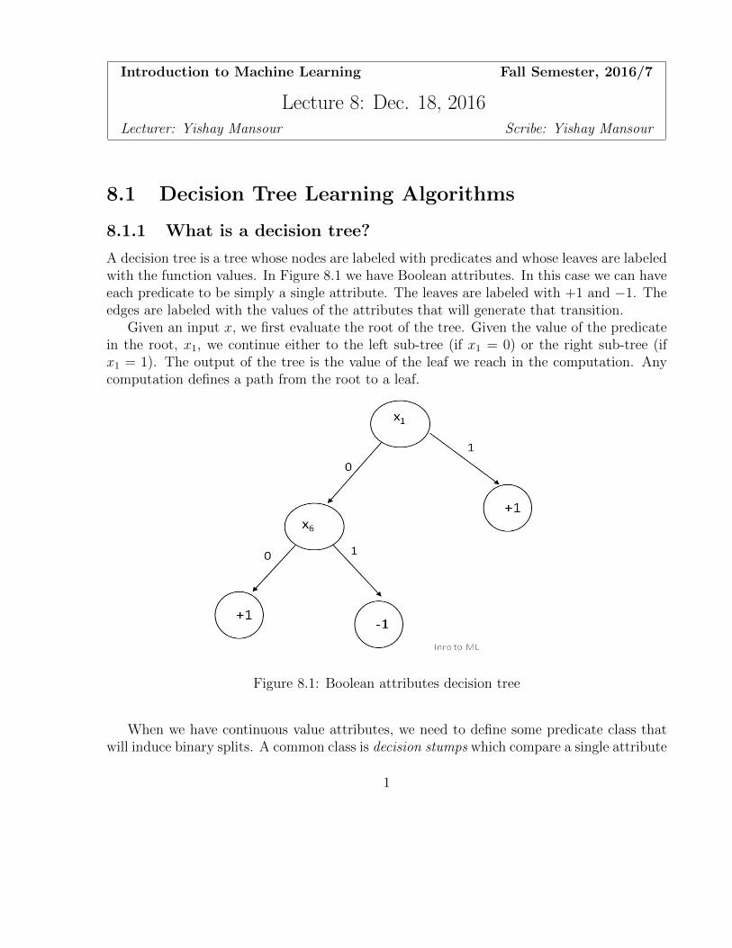
A decision tree is a tree whose nodes are labeled with predicates and whose leaves are labeledwith the function values. In Figure 8.1 we have Boolean attributes. In this case we can haveeach predicate to be simply a single attribute. The leaves are labeled with +1 and −1. Theedges are labeled with the values of the attributes that will generate that transition.

Given an input x, we first evaluate the root of the tree. Given the value of the predicatein the root, x1, we continue either to the left sub-tree (if x1 = 0) or the right sub-tree (ifx1 = 1). The output of the tree is the value of the leaf we reach in the computation. Anycomputation defines a path from the root to a leaf.

Figure 8.1: Boolean attributes decision tree

When we have continuous value attributes, we need to define some predicate class thatwill induce binary splits. A common class is decision stumps which compare a single attribute

1

2 Lecture 8

to a fixed value, e.g., x1 > 5. The evaluation, again, starts by evaluating the root, and followsa path until we reach a leaf. (See Figure 8.2)

Figure 8.2: A decision tree with decision stumps

When we consider decision stumps, the boundary for decisions are axis parallel, as shownin Figure 8.3.

Figure 8.3: Decision boundary for decision stumps.

8.1.2 Decision Trees - Basic setup

The decision tree would have a class of predicates H. This class of predicates can be decisionstumps, single attributes (in case of Boolean attributes) or any other predicate class. The

8.1. DECISION TREE LEARNING ALGORITHMS 3

predicate class H can be highly complicated (e.g., hyperplanes) but in most algorithms simpleclasses are used, since we like to build the decision trees from simple classifiers. Technically,we can have in each node even a large decision tree.

The input to the decision tree algorithm is the sample S = {(x, b)}, which as alwaysincludes examples of an input and its classification.

The output of the decision tree algorithm is a decision tree where each internal node hasa predicate from H and each leaf node has a classification value.

The goal is to output a small decision tree which classifies all (or most) of the examplescorrectly. This is inline with Occam’s Razor, which states that low complexity hypotheseshave a better generalization guarantee.

8.1.3 Decision Trees - Why?

One of the main reasons for using decision trees is human interpretability. Humans find itmuch easier to understand (small) decision trees. The evaluation process is very simple andone can understand fairly simply what the decision tree will predict.

There is a variety of efficient decision tree algorithms, and there are many commercialsoftware packages that learn decision trees, such as C4.5 or CART. Even Excel and MATLABhave a standard implementation of a decision tree algorithm.

The performance of decision trees is reasonable, probably slightly weaker than SVM andAdaBoost, but comparable on many data sets. Decision forests, which use many smalldecision trees have a general performance comparable to the best classification algorithms(including SVM and AdaBoost).

8.1.4 Decision Trees - VC dimension

We will compute the VC dimension as a function of the number of leaves s (which impliestree size 2s− 1) and the number of attributes n. We will denote it by V Cdim(s, n).

We start by computing the VC dimension in the case that the attributes are Boolean,i.e., the domain is {0, 1}n, and the splits are using single attributes. First we show thatV Cdim(s, n) ≥ s. For any set V of s examples, we can build a decision tree with s leavessuch that each leaf has a unique example reaching it. (Why is it possible?) Let TS be thetree, now for each assignment of labels to the set V we can set labels to the leaves and getthe desire assignment. Therefore, V Cdim(s, n) ≥ s.

For the upper bound, we consider the number of trees, the possible labeling of internalnodes and leaves. The number of trees is the Catalan number which gives 1

s+1

(2ss

)≤ 4s as an

upper bound on the number of trees. The number of assignments of attributes to internalnodes is ns−1 and the number of assignments of labels to the leaves is 2s. This bounds thenumber of trees by 4sns−12s ≤ (8n)s. Since the VC dimension is at most the logarithm ofthe size of the concept class, we have that V Cdim(s, n) ≤ s log(8n).

4 Lecture 8

For the general case, where the splitting criteria are from a hypothesis class of VC di-mension d, we will show that V Cdim(s, n) = O(sd log(sd)). The methodology is to boundthe number of functions on m examples, denoted by NF (m). For a shattered set of size mwe have 2m ≤ NF (m), and this will allow us to upper bound the VC dimension.

We will first fix the tree structure. (There are at most 4s such trees.) There are 2s

labeling to the leaves. For each tree and leaves labeling, we will build and m× s− 1 matrix,where the rows are labeled by inputs, and the columns are labeled by splitting functions.Note that given all the values of internal nodes we fix the path of an input. This impliesthat we need to count the number of different matrices. Using Sauer-Shelah lemma, for eachcolumn we have at most md different values. This bounds the number of matrices by mds.Assume we have m = V C(s, n) points which are shattered, this implies that 2m ≤ 4s2smds,and hence, V Cdim(s, n) = O(ds log(sd)).

8.1.5 Decision trees - Construction

There is a very natural greedy algorithm for constructing a decision tree given a sample. Wefirst decide on a predicate hr ∈ H to assign to the root. Once we selected hr, we split thesample S to two parts. In S0 (S1) we have all the examples where hr(x) = 0 (hr(x) = 1).Given S0 and S1 we can continue recursively to build a subtree for S0 and a subtree for S1.

The time complexity for such a procedure would be

Time(m) = O(|H|m) + Time(m0) + Time(m1)

where m = |S|, m0 = |S0| and m1 = |S1|. The worse case time is O(|H|m2), and in most casesthe running time is O(|H|m logm) since most of the splits will be approximately balanced.

The main issue that we need to resolve is how to select the predicate hr given a sampleS. Clearly, if all the samples have the same label we can select a leaf and mark it with thatlabel. Note that we are building a decision tree that would classify all the samples correctly.

8.1.6 Selecting predicates - splitting criteria

Given the outline of the greedy algorithm, the main remaining task is to select a predicate,assuming that not all the examples have the same label. We would like a simple local criteriathat would be based only on the parameters observed at the node.

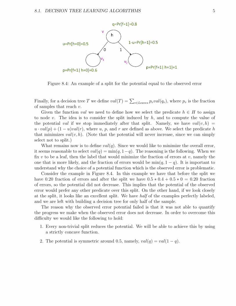
We would like to use a potential function val(·) to guide our selection. First let us defineval for a leaf v with a fraction of 1 equal to qv as val(qv). Next for an inner node v whichhas two leaf sons, we define val(v) = u · val(p) + (1− u)val(r), where u, p and r are definedas follows. Let u be the fraction of examples such that h(x) = 1, let p be the fraction ofexamples for which b = 1 (the target function is labeled 1) out of the examples with h(x) = 1,and let r be the fraction of examples for which b = 1 out of the examples with h(x) = 0.

8.1. DECISION TREE LEARNING ALGORITHMS 5

Figure 8.4: An example of a split for the potential equal to the observed error

Finally, for a decision tree T we define val(T ) =∑

v∈Leaves pvval(qv), where pv is the fractionof samples that reach v.

Given the function val we need to define how we select the predicate h ∈ H to assignto node v. The idea is to consider the split induced by h, and to compute the value ofthe potential val if we stop immediately after that split. Namely, we have val(v, h) =u · val(p) + (1− u)val(r), where u, p, and r are defined as above. We select the predicate hthat minimizes val(v, h). (Note that the potential will never increase, since we can simplyselect not to split.)

What remains now is to define val(q). Since we would like to minimize the overall error,it seems reasonable to select val(q) = min(q, 1−q). The reasoning is the following. When wefix v to be a leaf, then the label that would minimize the fraction of errors at v, namely theone that is more likely, and the fraction of errors would be min(q, 1− q). It is important tounderstand why the choice of a potential function which is the observed error is problematic.

Consider the example in Figure 8.4. In this example we have that before the split wehave 0.20 fraction of errors and after the split we have 0.5 ∗ 0.4 + 0.5 ∗ 0 = 0.20 fractionof errors, so the potential did not decrease. This implies that the potential of the observederror would prefer any other predicate over this split. On the other hand, if we look closelyat the split, it looks like an excellent split. We have half of the examples perfectly labeled,and we are left with building a decision tree for only half of the sample.

The reason why the observed error potential failed is that it was not able to quantifythe progress we make when the observed error does not decrease. In order to overcome thisdifficulty we would like the following to hold:

1. Every non-trivial split reduces the potential. We will be able to achieve this by usinga strictly concave function.

2. The potential is symmetric around 0.5, namely, val(q) = val(1− q).

6 Lecture 8

3. Potential zero implies perfect classification. This implies that val(0) = val(1) = 0.

4. We have val(0.5) = 0.5.

The important an interesting part is the strict concavity. The strict concavity will guar-antee us that any split will have a decrease in the potential. The reason is that

val(q) > u · val(p) + (1− u)val(r)

when q = up+ (1− u)r, due to the strict concavity.The other conditions are mainly to maintain normalization. Using them we can ensure

that val(T ) ≥ error(T ), since at any leaf v we will have val(v) > error(v).

8.1.7 Splitting criteria

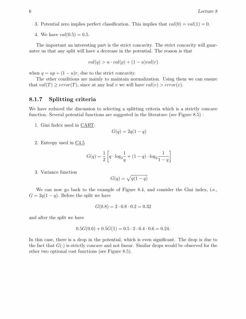
We have reduced the discussion to selecting a splitting criteria which is a strictly concavefunction. Several potential functions are suggested in the literature (see Figure 8.5) :

1. Gini Index used in CART:

G(q) = 2q(1− q)

2. Entropy used in C4.5

G(q) =1

2

[q · log2

1

q+ (1− q) · log2

1

1− q

]

3. Variance function

G(q) =√q(1− q)

We can now go back to the example of Figure 8.4, and consider the Gini index, i.e.,G = 2q(1− q). Before the split we have

G(0.8) = 2 · 0.8 · 0.2 = 0.32

and after the split we have

0.5G(0.6) + 0.5G(1) = 0.5 · 2 · 0.4 · 0.6 = 0.24.

In this case, there is a drop in the potential, which is even significant. The drop is due tothe fact that G(·) is strictly concave and not linear. Similar drops would be observed for theother two optional cost functions (see Figure 8.5).

8.1. DECISION TREE LEARNING ALGORITHMS 7

Figure 8.5: Relationships between different splitting criteria. The criteria, from inner toouter are observed error, Gini index, Entropy and Variance

8.1.8 Decision tree construction - putting it all together

We define a procedure DT (S), where S is the sample. The procedure returns a tree thatclassifies S correctly.

Procedure DT(S) return a decision tree TIf ∀(x, b) ∈ S we have b = 1 Then

Create a Leaf with label 1 and Return.If ∀(x, b) ∈ S we have b = 0 Then

Create a Leaf with label 0 and Return.For each h ∈ H compute

Sh = {(x, b) ∈ S|h(x) = 1}.uh = |Sh|/|S|Sh,1 = {(x, b) ∈ Sh|b = 1}ph = |Sh,1|/|Sh|.Sh,0 = {(x, b) ∈ S − Sh|b = 1}rh = |Sh,0|/|S − Sh|.val(h) = uhval(ph) + (1− uh)val(rh),

Let h′ = arg minh val(h).Let Sh′ = {x ∈ S : h′(x) = 1}.

8 Lecture 8

Call DT (Sh′) and receive T1.Call DT (S − Sh′) and receive T0.Return a decision tree with root labeled by h′, right subtree T1 and left subtree T0.

In class, in the slides we have an example of running the algorithm with the Gini index.

8.1.9 Decision tree algorithms - Guaranteed performance

We do not have any guarantee about the decision tree size produced by the greedy algorithm.In fact, if we consider the target function x1 ⊕ x2 and a uniform distribution over d binaryattributes then the greedy algorithm would create a very large decision tree. The reasonis that when it considers any single attribute, the probability that the target is 1 or 0 isidentical (until we select either x1 or x2). This implies that the decision tree will selectattributes randomly, until we select either x1 or x2.

In fact, we can show that finding the smallest decision tree is NP-hard, which means thatit is unlikely we will have a computationally efficient algorithm for computing the smallestdecision tree given a sample.

We can perform an analysis that is based on the weak learner hypothesis. The weaklearner hypothesis assumes that for any distribution there is a predicate h ∈ H which is aweak learner, i.e., has error at most 1/2 − γ. (We will study the weak learner hypothesisextensively next lecture.) Assuming the weak learner hypothesis we can bound the decisiontree size as a function of the parameter γ. Specifically,

1. For the Gini index,we have that the decision tree size is at most eO(1/γ21/ε2log21/ε).

2. For the Entropy index,we have that the decision tree size is at most eO(1/γ2log21/ε).

3. For the Variance index,we have that the decision tree size is at most eO(1/γ2log1/ε).

8.2 Decision Tree: Pruning

8.2.1 Why Pruning?

We saw the algorithm that builds a decision tree based on a sample. The decision tree isbuilt until zero training error. As we discussed many times before, our goal is to minimizethe testing error and not the training error.

In order to minimize the testing error, we have two basic options. The first option is todecide to do early stopping. Namely, stop building the decision tree at some point. Differentalternatives to perform the early stopping are: (1) when the number of examples in a nodeis small, (2) The reduction in the splitting criteria is small, (3) a bound on the number ofnodes, etc.

8.2. DECISION TREE: PRUNING 9

The alternative approach is to first build a large decision tree, until there is no trainingerror, and then prune the decision. The net effect is the same. In both cases we end witha small decision tree. The major difference is what we observe on the way. When we firstbuild a large tree, we may discover some important sub-structure that in case we stop early,we might miss. In some sense, we can always simulate the early stopping when we first buildthe large tree and then prune, but definitely cannot do the reverse.

8.2.2 Decision Tree Pruning: Problem Statement

The input to the decision tree pruning is a decision tree T . The output of the pruning isa decision tree T ′ which is derived from T . We will mainly look at the case where we canreplace an inner node of T by a leaf. Another, more advanced option, is to replace an innernode by the sub-tree rooted at one of its children. At the extreme, if we have no restrictionthen we are essentially left with the same problem we started with, finding a good decisiontree.

8.2.3 Reduced Error Pruning

In reduced error pruning we split the sample S to two parts S1 and S2. We use S1 to builda decision tree and use S2 for decisions of how to prune it. We do not assume anythingabout the building of the decision tree T using S1. (We do not even assume that the decisiontree T has zero error on S1, although in our main application this will be the case.) Ourpruning will use S2 to modify the structure of T . The pruning of an internal node v is doneby replacing the sub-tree rooted at v by a leaf.

In the pruning we traverse the tree bottom-up and for each internal node v we checkwhether we want to replace the sub-tree originated by it with a leaf or not. The decisionof whether to prune the node v or not is rather simple: we sum the errors of the leaves inthe sub-tree rooted by node v and the errors in case we replace it with a leaf. If replacingthe sub-tree rooted at v will reduce the total error on S2 we prune v. In case the number oferrors is the same we also prune the node in order to minimize the size of the decision treewe output. Otherwise, we keep the node (and the sub-tree rooted at it).

Notice that on each step in the pruning algorithm we examine the sub-tree that is relevantto the current stage in the algorithm, meaning that if we pruned part of the sub-tree rootedin v on previous iterations then when we check v we examine it against its current sub-treeand not the original one. The pruning of an internal node v is done by replacing the sub-treerooted at v by a leaf at v.

10 Lecture 8

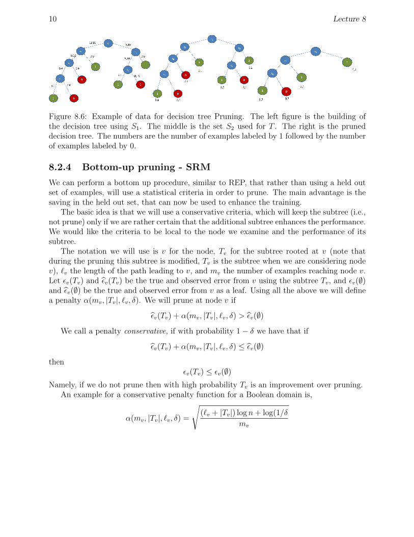
Figure 8.6: Example of data for decision tree Pruning. The left figure is the building ofthe decision tree using S1. The middle is the set S2 used for T . The right is the pruneddecision tree. The numbers are the number of examples labeled by 1 followed by the numberof examples labeled by 0.

8.2.4 Bottom-up pruning - SRM

We can perform a bottom up procedure, similar to REP, that rather than using a held outset of examples, will use a statistical criteria in order to prune. The main advantage is thesaving in the held out set, that can now be used to enhance the training.

The basic idea is that we will use a conservative criteria, which will keep the subtree (i.e.,not prune) only if we are rather certain that the additional subtree enhances the performance.We would like the criteria to be local to the node we examine and the performance of itssubtree.

The notation we will use is v for the node, Tv for the subtree rooted at v (note thatduring the pruning this subtree is modified, Tv is the subtree when we are considering nodev), `v the length of the path leading to v, and mv the number of examples reaching node v.Let εv(Tv) and ε̂v(Tv) be the true and observed error from v using the subtree Tv, and εv(∅)and ε̂v(∅) be the true and observed error from v as a leaf. Using all the above we will definea penalty α(mv, |Tv|, `v, δ). We will prune at node v if

ε̂v(Tv) + α(mv, |Tv|, `v, δ) > ε̂v(∅)

We call a penalty conservative, if with probability 1− δ we have that if

ε̂v(Tv) + α(mv, |Tv|, `v, δ) ≤ ε̂v(∅)

thenεv(Tv) ≤ εv(∅)

Namely, if we do not prune then with high probability Tv is an improvement over pruning.An example for a conservative penalty function for a Boolean domain is,

α(mv, |Tv|, `v, δ) =

√(`v + |Tv|) log n+ log(1/δ

mv

8.2. DECISION TREE: PRUNING 11

We can give a theoretical guarantee on this pruning (although we will give only the high-lights). First we can show the following simple claim that follows from the conservativenessof the penalty. Let Topt be the best pruning and Tsrm the pruning using the SRM criteria.Then with high probability Tsrm is a subtree of Topt.

The main result is to bound the difference between the error of Tsrm and Topt. We canshow the following relationship,

ε(Tsrm)− ε(Topt) ≤√|Toptm

O(log(|Topt|/δ) + hopt log(nm/δ)),

where hoptg is the height of Topt.

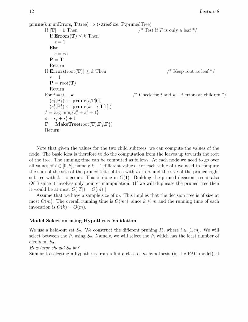
8.2.5 Model Selection

In this section we present an algorithm that produces few pruning possibilities. The algo-rithm will be wrapped by a model selection procedure (either Structural Risk Minimization,Hypothesis Validation, or any other) that chooses one of the pruning possibilities producedby the underlying algorithm. Generally the core algorithm will be given a decision tree Tand target number of errors e and will produce the smallest pruned trees that has such errorsrate. This algorithm is an instance of dynamic programming, where the main parameter isthe number of errors.

Algorithm

1. Build a tree T using S.

2. For each e, compute the minimal pruning size ke (and a pruned decision tree Te) withat most e errors.

3. Select one pruning using some criteria.

We will first show how to find the pruning that will minimize the decision tree size for agiven number of errors. (Or alternatively, find the pruning that for a given tree size minimizesthe number of errors.)

Finding the minimum pruning

Given e, the number of errors, we want to find the smallest pruned version of T that hasat most e errors. We give a dynamic programming algorithm. We use T[0] and T[1] torepresent the left and right child subtrees of T respectively. We denote by root(T) the rootnode of the tree T. We also define tree(r,T0,T1) to be the tree formed by making thesubtrees T0 and T1 the left and right child of the root node r. For every node v of T,Errors(v) is the number of classification errors on the sample set of v as a leaf.

12 Lecture 8

prune(k:numErrors, T:tree) ⇒ (s:treeSize, P:prunedTree)If |T| = 1 Then /* Test if T is only a leaf */

If Errors(T) ≤ k Thens = 1

Elses =∞

P = TReturn

If Errors(root(T)) ≤ k Then /* Keep root as leaf */s = 1P = root(T)Return

For i = 0 . . . k /* Check for i and k − i errors at children */(s0i ,P

0i ) ← prune(i,T[0])

(s1i ,P1i ) ← prune(k − i,T[1],)

I = arg mini{s0i + s1i + 1}s = s0I + s1I + 1P = MakeTree(root(T),P0

I ,P1I)

Return

Note that given the values for the two child subtrees, we can compute the values of thenode. The basic idea is therefore to do the computation from the leaves up towards the rootof the tree. The running time can be computed as follows. At each node we need to go overall values of i ∈ [0, k], namely k+ 1 different values. For each value of i we need to computethe sum of the size of the pruned left subtree with i errors and the size of the pruned rightsubtree with k − i errors. This is done in O(1). Building the pruned decision tree is alsoO(1) since it involves only pointer manipulation. (If we will duplicate the pruned tree thenit would be at most O(|T |) = O(m).)

Assume that we have a sample size of m. This implies that the decision tree is of size atmost O(m). The overall running time is O(m2), since k ≤ m and the running time of eachinvocation is O(k) = O(m).

Model Selection using Hypothesis Validation

We use a held-out set S2. We construct the different pruning Pi, where i ∈ [1,m]. We willselect between the Pi using S2. Namely, we will select the Pi which has the least number oferrors on S2.How large should S2 be?Similar to selecting a hypothesis from a finite class of m hypothesis (in the PAC model), if

8.3. BIBLIOGRAPHIC NOTES 13

we set |S2| = 1ε2

log mδ

then with probability 1− δ we have for each Pi a deviation of at mostε in estimating the error of Pi. This implies that with probability 1− δ the pruning Pi whichminimizes the observed error of S2 has true error of at most 2ε more than the true error ofthe best pruning Pj.

Model Selection using Structural Risk Minimization

We have a set of prunings Pi, for i ∈ [1,m]. We will select between them using the existingexamples, and not use another set of examples. The Structural Risk Minimization (SRM)will use the following decision rule,

P ∗i = argminPi

{error(Pi) +

√|Pi|m

}

Model selection - Summary

The main drawback of this approach is the running time, which is quadratic in the samplesize. This implies that for a large data set the approach will not be feasible. The benefit isthat in case of small data sets it allows to utilize much better the examples we have.

8.3 Bibliographic Notes

The following papers have been used for this leacture notes, and have additional proofs whichare missing from this scribe notes.

1. Michael J. Kearns, Yishay Mansour: On the Boosting Ability of Top-Down DecisionTree Learning Algorithms. J. Comput. Syst. Sci. 1999 (preliminary version STOC1996).

2. Yishay Mansour: Pessimistic decision tree pruning based Continuous-time. ICML 1997

3. Michael J. Kearns and Yishay Mansour: A Fast, Bottom-Up Decision Tree PruningAlgorithm with Near-Optimal Generalization. ICML 1998