8.1 2D plane strain plasticity - MIDAS...
49
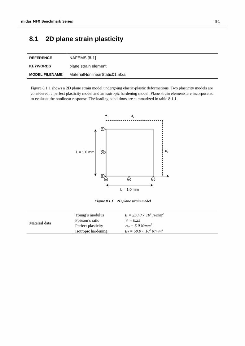
1 midas NFX Benchmark Series 8-1 8.1 2D plane strain plasticity REFERENCE NAFEMS [8-1] KEYWORDS plane strain element MODEL FILENAME MaterialNonlinearStatic01.nfxa Figure 8.1.1 2D plane strain model Material data Young’ s modulus Poisson’ s ratio Perfect plasticity Isotropic hardening E = 250.0 10 3 N/mm 2 = 0.25 Y = 5.0 N/mm 2 E T = 50.0 10 3 N/mm 2 L = 1.0 mm u y u x L = 1.0 mm Figure 8.1.1 shows a 2D plane strain model undergoing elastic-plastic deformations. Two plasticity models are considered; a perfect plasticity model and an isotropic hardening model. Plane strain elements are incorporated to evaluate the nonlinear response. The loading conditions are summarized in table 8.1.1.
Transcript of 8.1 2D plane strain plasticity - MIDAS...
1
midas NFX Benchmark Series 8-1
8.1 2D plane strain plasticity
REFERENCE NAFEMS [8-1]
KEYWORDS plane strain element
MODEL FILENAME MaterialNonlinearStatic01.nfxa
Figure 8.1.1 2D plane strain model
Material data
Young’s modulus
Poisson’s ratio
Perfect plasticity
Isotropic hardening
E = 250.0 103 N/mm
2
= 0.25
Y = 5.0 N/mm2
ET = 50.0 103 N/mm
2
L = 1.0 mm
A B
CD
uy
uxL = 1.0 mm
Figure 8.1.1 shows a 2D plane strain model undergoing elastic-plastic deformations. Two plasticity models are
considered; a perfect plasticity model and an isotropic hardening model. Plane strain elements are incorporated
to evaluate the nonlinear response. The loading conditions are summarized in table 8.1.1.
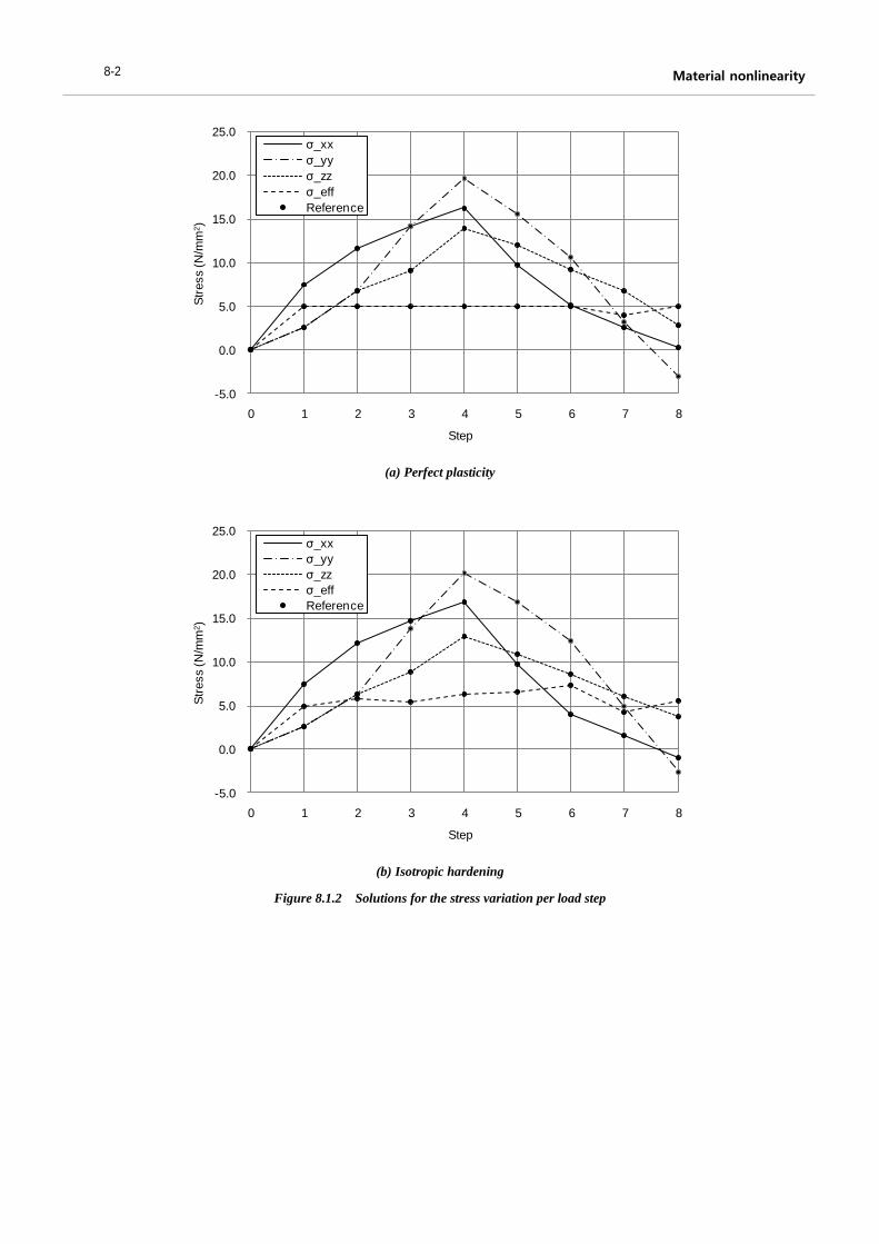
Material nonlinearity 8-2
(a) Perfect plasticity
(b) Isotropic hardening
Figure 8.1.2 Solutions for the stress variation per load step
-5.0
0.0
5.0
10.0
15.0
20.0
25.0
0 1 2 3 4 5 6 7 8
Str
ess (N
/mm
2)
Step
σ_xx
σ_yy
σ_zz
σ_eff
Reference
-5.0
0.0
5.0
10.0
15.0
20.0
25.0
0 1 2 3 4 5 6 7 8
Str
ess (N
/mm
2)
Step
σ_xx
σ_yy
σ_zz
σ_eff
Reference
3
midas NFX Benchmark Series 8-3
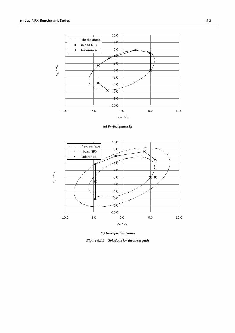
(a) Perfect plasticity
(b) Isotropic hardening
Figure 8.1.3 Solutions for the stress path
-10.0
-8.0
-6.0
-4.0
-2.0
0.0
2.0
4.0
6.0
8.0
10.0
-10.0 -5.0 0.0 5.0 10.0
σy
y -σ
zz
σxx - σzz
Yield surface
midas NFX
Reference
-10.0
-8.0
-6.0
-4.0
-2.0
0.0
2.0
4.0
6.0
8.0
10.0
-10.0 -5.0 0.0 5.0 10.0
σy
y -σ
zz
σxx - σzz
Yield surface
midas NFX
Reference
Material nonlinearity 8-4
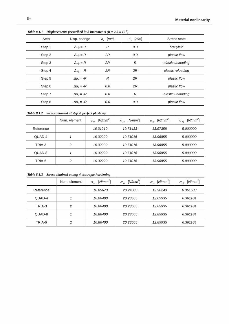
Table 8.1.1 Displacements prescribed in 8 increments (R = 2.5 10-5)
Table 8.1.2 Stress obtained at step 4, perfect plasticity
Table 8.1.3 Stress obtained at step 4, isotropic hardening
Step Disp. change x [mm] y [mm] Stress state
Step 1 Δux = R R 0.0 first yield
Step 2 Δux = R 2R 0.0 plastic flow
Step 3 Δuy = R 2R R elastic unloading
Step 4 Δuy = R 2R 2R plastic reloading
Step 5 Δux = -R R 2R plastic flow
Step 6 Δux = -R 0.0 2R plastic flow
Step 7 Δuy = -R 0.0 R elastic unloading
Step 8 Δuy = -R 0.0 0.0 plastic flow
Num. element xx [N/mm2] yy [N/mm
2] zz [N/mm
2] eff [N/mm
2]
Reference 16.31210 19.71433 13.97358 5.000000
QUAD-4 1 16.32229 19.71016 13.96855 5.000000
TRIA-3 2 16.32229 19.71016 13.96855 5.000000
QUAD-8 1 16.32229 19.71016 13.96855 5.000000
TRIA-6 2 16.32229 19.71016 13.96855 5.000000
Num. element xx [N/mm2] yy [N/mm
2] zz [N/mm
2] eff [N/mm
2]
Reference 16.85673 20.24083 12.90243 6.361633
QUAD-4 1 16.86400 20.23665 12.89935 6.361184
TRIA-3 2 16.86400 20.23665 12.89935 6.361184
QUAD-8 1 16.86400 20.23665 12.89935 6.361184
TRIA-6 2 16.86400 20.23665 12.89935 6.361184

5
midas NFX Benchmark Series 8-5
8.2 2D plane stress plasticity
REFERENCE NAFEMS [8-1]
KEYWORDS plane stress element
MODEL FILENAME MaterialNonlinearStatic02.nfxa
Figure 8.2.1 2D plane stress model
Material data
Young’s modulus
Poisson’s ratio
Perfect plasticity
Isotropic hardening
E = 250.0 103 N/mm
2
= 0.25
Y = 5.0 N/mm2
ET = 50.0 103 N/mm
2
L = 1.0 mm
A B
CD
uy
uxL = 1.0 mm
Figure 8.2.1 shows a 2D plane stress model undergoing elastic-plastic deformations. Two plasticity models are
considered; a perfect plastic model and an isotropic hardening model. Material nonlinear analyses are carried
out using plane stress elements in accordance with the loading condition summarized in table 8.2.1.
Material nonlinearity 8-6
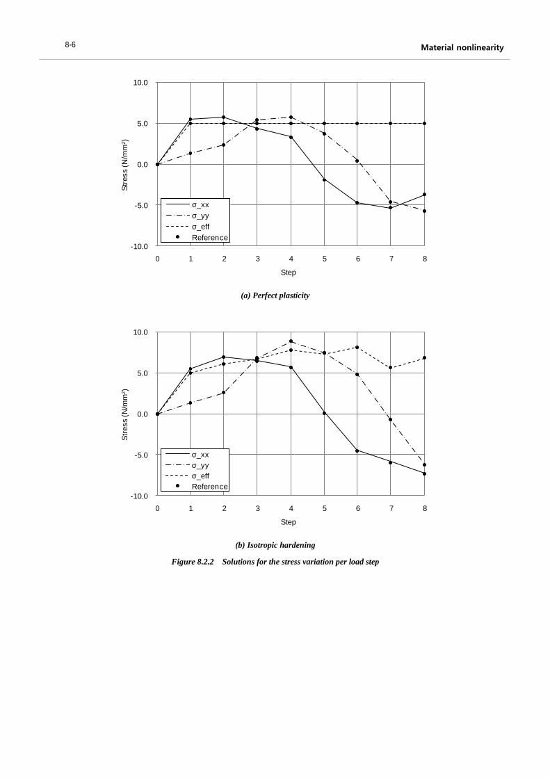
(a) Perfect plasticity
(b) Isotropic hardening
Figure 8.2.2 Solutions for the stress variation per load step
-10.0
-5.0
0.0
5.0
10.0
0 1 2 3 4 5 6 7 8
Str
ess (N
/mm
2)
Step
σ_xx
σ_yy
σ_eff
Reference
-10.0
-5.0
0.0
5.0
10.0
0 1 2 3 4 5 6 7 8
Str
ess (N
/mm
2)
Step
σ_xx
σ_yy
σ_eff
Reference

7
midas NFX Benchmark Series 8-7
(a) Perfect plasticity
(b) Isotropic hardening
Figure 8.2.3 Solutions for the stress path
-10.0
-8.0
-6.0
-4.0
-2.0
0.0
2.0
4.0
6.0
8.0
10.0
-10.0 -8.0 -6.0 -4.0 -2.0 0.0 2.0 4.0 6.0 8.0 10.0
σy
y-σ
zz
σxx - σzz
Yield surface
midas NFX
Reference
-10.0
-8.0
-6.0
-4.0
-2.0
0.0
2.0
4.0
6.0
8.0
10.0
-10.0 -8.0 -6.0 -4.0 -2.0 0.0 2.0 4.0 6.0 8.0 10.0
σy
y-σ
zz
σxx - σzz
Yield surface
midas NFX
Reference
Material nonlinearity 8-8
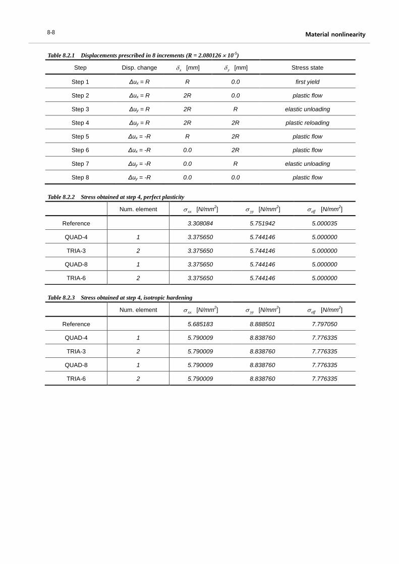
Table 8.2.1 Displacements prescribed in 8 increments (R = 2.080126 10-5)
Table 8.2.2 Stress obtained at step 4, perfect plasticity
Table 8.2.3 Stress obtained at step 4, isotropic hardening
Step Disp. change x [mm] y [mm] Stress state
Step 1 Δux = R R 0.0 first yield
Step 2 Δux = R 2R 0.0 plastic flow
Step 3 Δuy = R 2R R elastic unloading
Step 4 Δuy = R 2R 2R plastic reloading
Step 5 Δux = -R R 2R plastic flow
Step 6 Δux = -R 0.0 2R plastic flow
Step 7 Δuy = -R 0.0 R elastic unloading
Step 8 Δuy = -R 0.0 0.0 plastic flow
Num. element xx [N/mm2] yy [N/mm
2] eff [N/mm
2]
Reference 3.308084 5.751942 5.000035
QUAD-4 1 3.375650 5.744146 5.000000
TRIA-3 2 3.375650 5.744146 5.000000
QUAD-8 1 3.375650 5.744146 5.000000
TRIA-6 2 3.375650 5.744146 5.000000
Num. element xx [N/mm2] yy [N/mm
2] eff [N/mm
2]
Reference 5.685183 8.888501 7.797050
QUAD-4 1 5.790009 8.838760 7.776335
TRIA-3 2 5.790009 8.838760 7.776335
QUAD-8 1 5.790009 8.838760 7.776335
TRIA-6 2 5.790009 8.838760 7.776335
9
midas NFX Benchmark Series 8-9
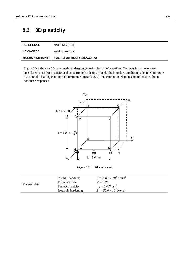
8.3 3D plasticity
REFERENCE NAFEMS [8-1]
KEYWORDS solid elements
MODEL FILENAME MaterialNonlinearStatic03.nfxa
Figure 8.3.1 3D solid model
Material data
Young’s modulus
Poisson’s ratio
Perfect plasticity
Isotropic hardening
E = 250.0 103 N/mm
2
= 0.25
Y = 5.0 N/mm2
ET = 50.0 103 N/mm
2
L = 1.0 mm
A B
CD
uz
ux
E F
GH
Z
X
Y
uy
L = 1.0 mm
L = 1.0 mm
Figure 8.3.1 shows a 3D cube model undergoing elastic-plastic deformations. Two plasticity models are
considered; a perfect plasticity and an isotropic hardening model. The boundary condition is depicted in figure
8.3.1 and the loading condition is summarized in table 8.3.1. 3D continuum elements are utilized to obtain
nonlinear responses.
Material nonlinearity 8-10
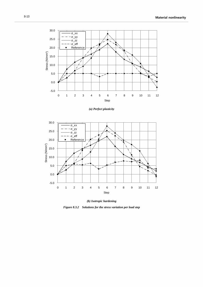
(a) Perfect plasticity
(b) Isotropic hardening
Figure 8.3.2 Solutions for the stress variation per load step
-5.0
0.0
5.0
10.0
15.0
20.0
25.0
30.0
0 1 2 3 4 5 6 7 8 9 10 11 12
Str
ess (N
/mm
2)
Step
σ_xx
σ_yy
σ_zz
σ_eff
Reference
-5.0
0.0
5.0
10.0
15.0
20.0
25.0
30.0
0 1 2 3 4 5 6 7 8 9 10 11 12
Str
ess (N
/mm
2)
Step
σ_xx
σ_yy
σ_zz
σ_eff
Reference
11
midas NFX Benchmark Series 8-11
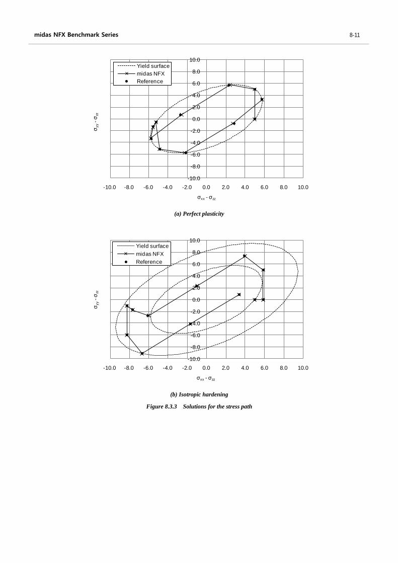
(a) Perfect plasticity
(b) Isotropic hardening
Figure 8.3.3 Solutions for the stress path
-10.0
-8.0
-6.0
-4.0
-2.0
0.0
2.0
4.0
6.0
8.0
10.0
-10.0 -8.0 -6.0 -4.0 -2.0 0.0 2.0 4.0 6.0 8.0 10.0
σy
y-σ
zz
σxx - σzz
Yield surface
midas NFX
Reference
-10.0
-8.0
-6.0
-4.0
-2.0
0.0
2.0
4.0
6.0
8.0
10.0
-10.0 -8.0 -6.0 -4.0 -2.0 0.0 2.0 4.0 6.0 8.0 10.0
σy
y-σ
zz
σxx - σzz
Yield surface
midas NFX
Reference
Material nonlinearity 8-12
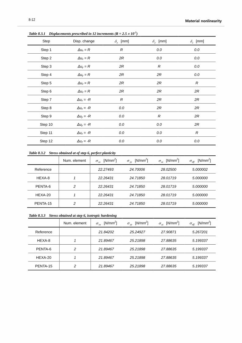
Table 8.3.1 Displacements prescribed in 12 increments (R = 2.5 10-5)
Table 8.3.2 Stress obtained at of step 6, perfect plasticity
Table 8.3.3 Stress obtained at step 6, isotropic hardening
Step Disp. change x [mm] y [mm] z [mm]
Step 1 Δux = R R 0.0 0.0
Step 2 Δux = R 2R 0.0 0.0
Step 3 Δuy = R 2R R 0.0
Step 4 Δuy = R 2R 2R 0.0
Step 5 Δuz = R 2R 2R R
Step 6 Δuz = R 2R 2R 2R
Step 7 Δux = -R R 2R 2R
Step 8 Δux = -R 0.0 2R 2R
Step 9 Δuy = -R 0.0 R 2R
Step 10 Δuy = -R 0.0 0.0 2R
Step 11 Δuz = -R 0.0 0.0 R
Step 12 Δuz = -R 0.0 0.0 0.0
Num. element xx [N/mm2] yy [N/mm
2] zz [N/mm
2] eff [N/mm
2]
Reference 22.27493 24.70006 28.02500 5.000002
HEXA-8 1 22.26431 24.71850 28.01719 5.000000
PENTA-6 2 22.26431 24.71850 28.01719 5.000000
HEXA-20 1 22.26431 24.71850 28.01719 5.000000
PENTA-15 2 22.26431 24.71850 28.01719 5.000000
Num. element xx [N/mm2] yy [N/mm
2] zz [N/mm
2] eff [N/mm
2]
Reference 21.84202 25.24927 27.90871 5.267201
HEXA-8 1 21.89467 25.21898 27.88635 5.199337
PENTA-6 2 21.89467 25.21898 27.88635 5.199337
HEXA-20 1 21.89467 25.21898 27.88635 5.199337
PENTA-15 2 21.89467 25.21898 27.88635 5.199337
13
midas NFX Benchmark Series 8-13
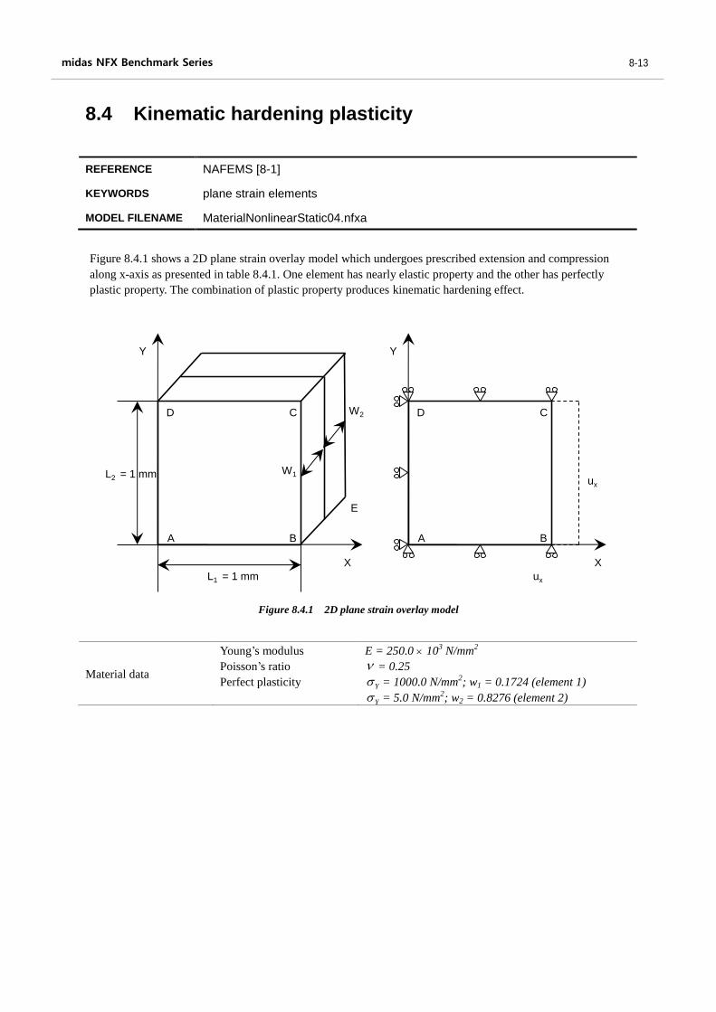
8.4 Kinematic hardening plasticity
REFERENCE NAFEMS [8-1]
KEYWORDS plane strain elements
MODEL FILENAME MaterialNonlinearStatic04.nfxa
Figure 8.4.1 2D plane strain overlay model
Material data
Young’s modulus
Poisson’s ratio
Perfect plasticity
E = 250.0 103 N/mm
2
= 0.25
Y = 1000.0 N/mm2; w1 = 0.1724 (element 1)
Y = 5.0 N/mm2; w2 = 0.8276 (element 2)
L1 = 1 mm
A B
CD
ux
E
W1
X
Y
W2
A B
CD
L2 = 1 mmux
X
Y
Figure 8.4.1 shows a 2D plane strain overlay model which undergoes prescribed extension and compression
along x-axis as presented in table 8.4.1. One element has nearly elastic property and the other has perfectly
plastic property. The combination of plastic property produces kinematic hardening effect.
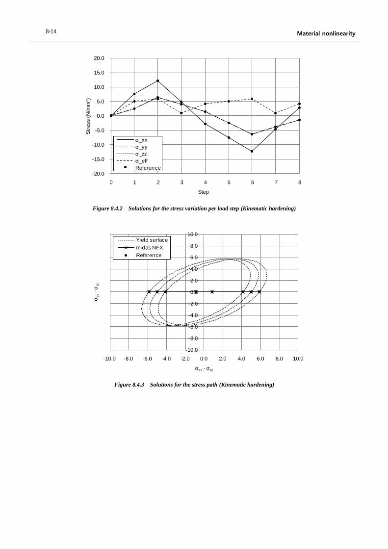
Material nonlinearity 8-14
Figure 8.4.2 Solutions for the stress variation per load step (Kinematic hardening)
Figure 8.4.3 Solutions for the stress path (Kinematic hardening)
-20.0
-15.0
-10.0
-5.0
0.0
5.0
10.0
15.0
20.0
0 1 2 3 4 5 6 7 8
Str
ess (N
/mm
2)
Step
σ_xx
σ_yy
σ_zz
σ_eff
Reference
-10.0
-8.0
-6.0
-4.0
-2.0
0.0
2.0
4.0
6.0
8.0
10.0
-10.0 -8.0 -6.0 -4.0 -2.0 0.0 2.0 4.0 6.0 8.0 10.0
σy
y-σ
zz
σxx - σzz
Yield surface
midas NFX
Reference
15
midas NFX Benchmark Series 8-15
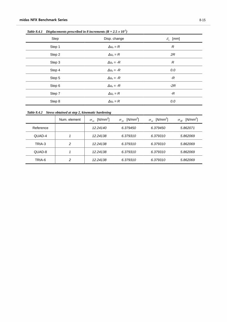
Table 8.4.1 Displacements prescribed in 8 increments (R = 2.5 10-5)
Table 8.4.2 Stress obtained at step 2, kinematic hardening
Step Disp. change x [mm]
Step 1 Δux = R R
Step 2 Δux = R 2R
Step 3 Δux = -R R
Step 4 Δux = -R 0.0
Step 5 Δux = -R -R
Step 6 Δux = -R -2R
Step 7 Δux = R -R
Step 8 Δux = R 0.0
Num. element xx [N/mm2] yy [N/mm
2] zz [N/mm
2] eff [N/mm
2]
Reference 12.24140 6.379450 6.379450 5.862071
QUAD-4 1 12.24138 6.379310 6.379310 5.862069
TRIA-3 2 12.24138 6.379310 6.379310 5.862069
QUAD-8 1 12.24138 6.379310 6.379310 5.862069
TRIA-6 2 12.24138 6.379310 6.379310 5.862069
Material nonlinearity 8-16
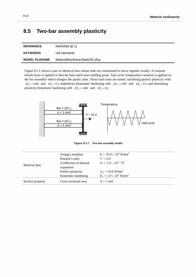
8.5 Two-bar assembly plasticity
REFERENCE NAFEMS [8-1]
KEYWORDS rod elements
MODEL FILENAME MaterialNonlinearStatic05.nfxa
Figure 8.5.1 Two-bar assembly model
Material data
Young’s modulus
Poisson’s ratio
Coefficient of thermal
expansion
Perfect plasticity
Kinematic hardening
E = 10.0 103 N/mm
2
= 0.0
= 1.0 10-5
/°C
Y = 10.0 N/mm2
ET = 1.0 103 N/mm
2
Section property Cross-sectional area A = 1 mm2
Bar 1 (ΔT1)
P = 15.0
Bar 2 (ΔT2)
Temperature
Half-cycleA = 1 mm2
A = 1 mm2
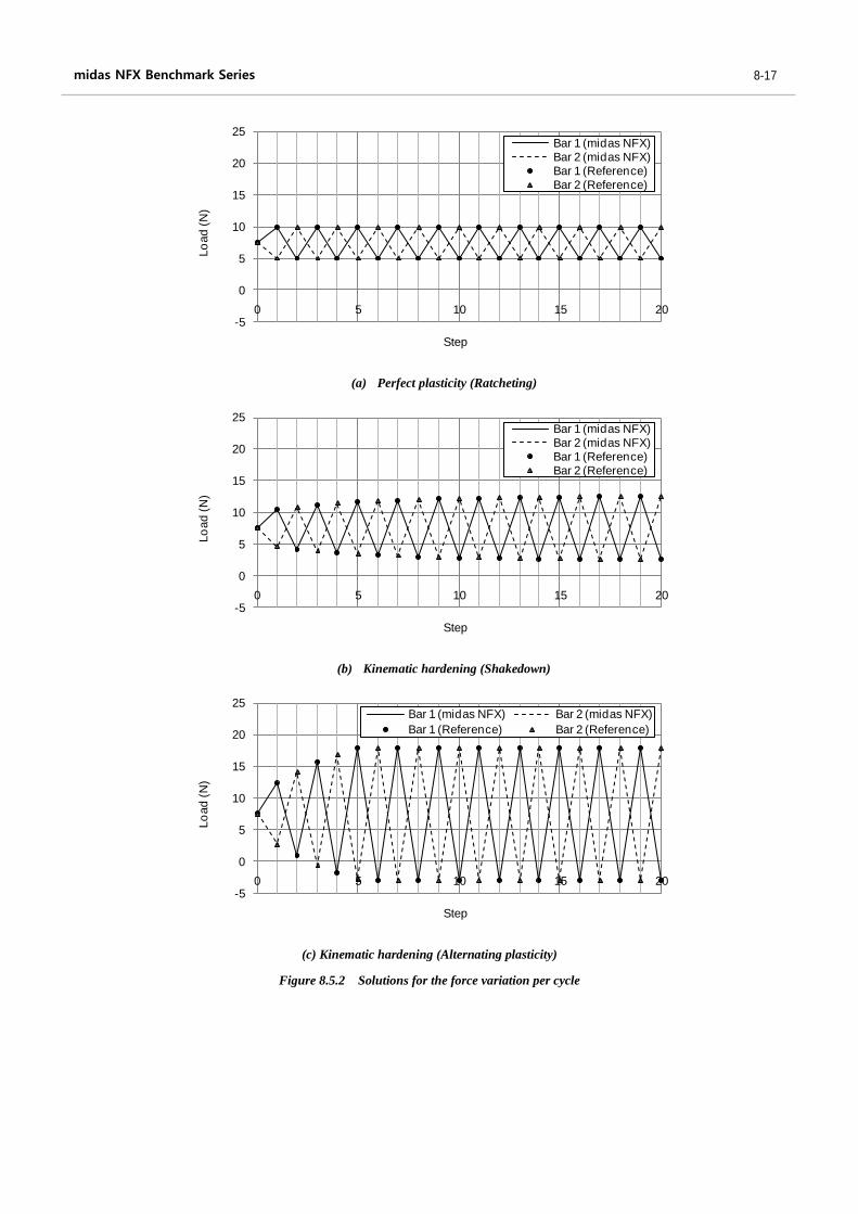
Figure 8.5.1 shows a pair of identical bars whose ends are constrained to move together axially. A constant
tensile force is applied so that the bars reach near-yielding point. And cyclic temperature variation is applied on
the bar assembly which changes the plastic state. Three load cases are tested; ratcheting (perfect plasticity with
1 100T and 2 0T ), shakedown (kinematic hardening with 1 100T and 2 0T ), and alternating
plasticity (kinematic hardening with 1 300T and 2 0T ).
17
midas NFX Benchmark Series 8-17
(a) Perfect plasticity (Ratcheting)
(b) Kinematic hardening (Shakedown)
(c) Kinematic hardening (Alternating plasticity)
Figure 8.5.2 Solutions for the force variation per cycle
-5
0
5
10
15
20
25
0 5 10 15 20
Lo
ad
(N
)
Step
Bar 1 (midas NFX)Bar 2 (midas NFX)Bar 1 (Reference)Bar 2 (Reference)
-5
0
5
10
15
20
25
0 5 10 15 20
Lo
ad
(N
)
Step
Bar 1 (midas NFX)Bar 2 (midas NFX)Bar 1 (Reference)Bar 2 (Reference)
-5
0
5
10
15
20
25
0 5 10 15 20
Lo
ad
(N
)
Step
Bar 1 (midas NFX) Bar 2 (midas NFX)
Bar 1 (Reference) Bar 2 (Reference)
Material nonlinearity 8-18
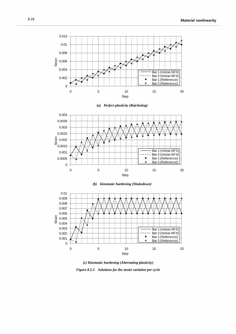
(a) Perfect plasticity (Ratcheting)
(b) Kinematic hardening (Shakedown)
(c) Kinematic hardening (Alternating plasticity)
Figure 8.5.3 Solutions for the strain variation per cycle
0
0.002
0.004
0.006
0.008
0.01
0.012
0 5 10 15 20
Str
ain
Step
Bar 1 (midas NFX)Bar 2 (midas NFX)Bar 1 (Reference)Bar 2 (Reference)
0
0.0005
0.001
0.0015
0.002
0.0025
0.003
0.0035
0.004
0 5 10 15 20
Str
ain
Step
Bar 1 (midas NFX)Bar 2 (midas NFX)Bar 1 (Reference)Bar 2 (Reference)
0
0.001
0.002
0.003
0.004
0.005
0.006
0.007
0.008
0.009
0.01
0 5 10 15 20
Str
ain
Step
Bar 1 (midas NFX)Bar 2 (midas NFX)Bar 1 (Reference)Bar 2 (Reference)

19
midas NFX Benchmark Series 8-19
(a) Perfect plasticity (Ratcheting)
(b) Kinematic hardening (Shakedown)
(c) Kinematic hardening (Alternating plasticity)
Figure 8.5.4 Solutions for the load-strain curve
-5
0
5
10
15
20
25
0 0.002 0.004 0.006 0.008 0.01 0.012
Lo
ad
(N
)
Strain
Bar 1 (midas NFX)Bar 2 (midas NFX)Bar 1 (Reference)Bar 2 (Reference)
-5
0
5
10
15
20
25
0 0.0005 0.001 0.0015 0.002 0.0025 0.003 0.0035
Lo
ad
(N
)
Strain
Bar 1 (midas NFX)Bar 2 (midas NFX)Bar 1 (Reference)Bar 2 (Reference)
-5
0
5
10
15
20
25
0 0.001 0.002 0.003 0.004 0.005 0.006 0.007 0.008 0.009
Lo
ad
(N
)
Strain
Bar 1 (midas NFX)Bar 2 (midas NFX)Bar 1 (Reference)Bar 2 (Reference)
Material nonlinearity 8-20
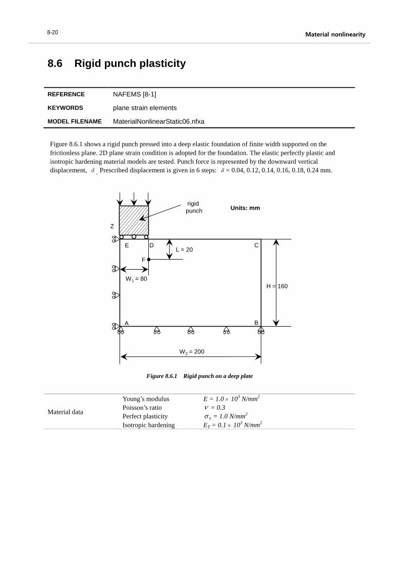
8.6 Rigid punch plasticity
REFERENCE NAFEMS [8-1]
KEYWORDS plane strain elements
MODEL FILENAME MaterialNonlinearStatic06.nfxa
Figure 8.6.1 Rigid punch on a deep plate
Material data
Young’s modulus
Poisson’s ratio
Perfect plasticity
Isotropic hardening
E = 1.0 103 N/mm
2
= 0.3
Y = 1.0 N/mm2
ET = 0.1 103 N/mm
2
A B
CD
Z
H = 160
W2 = 200
E
F
L = 20
W1 = 80
rigid
punchUnits: mm
Figure 8.6.1 shows a rigid punch pressed into a deep elastic foundation of finite width supported on the
frictionless plane. 2D plane strain condition is adopted for the foundation. The elastic perfectly plastic and
isotropic hardening material models are tested. Punch force is represented by the downward vertical
displacement, . Prescribed displacement is given in 6 steps: = 0.04, 0.12, 0.14, 0.16, 0.18, 0.24 mm.
21
midas NFX Benchmark Series 8-21
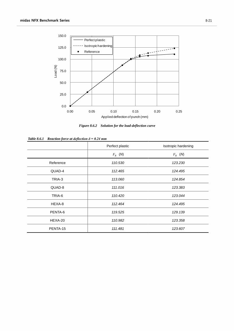
Figure 8.6.2 Solution for the load-deflection curve
Table 8.6.1 Reaction force at deflection δ = 0.24 mm
0.0
25.0
50.0
75.0
100.0
125.0
150.0
0.00 0.05 0.10 0.15 0.20 0.25
Lo
ad
(N
)
Applied deflection of punch (mm)
Perfect plastic
Isotropic hardening
Reference
Perfect plastic Isotropic hardening
RF (N) RF (N)
Reference 110.530 123.230
QUAD-4 112.465 124.495
TRIA-3 113.060 124.854
QUAD-8 111.016 123.383
TRIA-6 110.420 123.044
HEXA-8 112.464 124.495
PENTA-6 119.525 129.139
HEXA-20 110.982 123.358
PENTA-15 111.481 123.607
Material nonlinearity 8-22
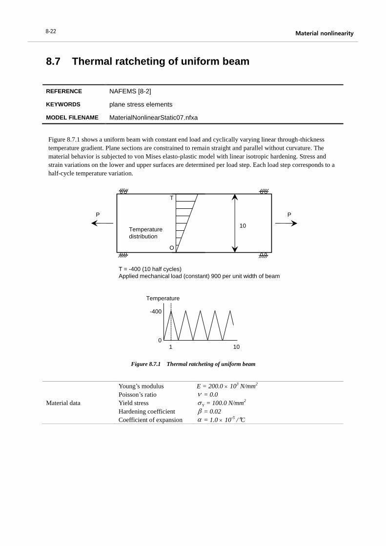
8.7 Thermal ratcheting of uniform beam
REFERENCE NAFEMS [8-2]
KEYWORDS plane stress elements
MODEL FILENAME MaterialNonlinearStatic07.nfxa
Figure 8.7.1 Thermal ratcheting of uniform beam
Material data
Young’s modulus
Poisson’s ratio
Yield stress
Hardening coefficient
Coefficient of expansion
E = 200.0 103 N/mm
2
= 0.0
Y = 100.0 N/mm2
= 0.02
= 1.0 10-5
/°C
Temperature
distribution
T = -400 (10 half cycles)
Applied mechanical load (constant) 900 per unit width of beam
O
10
P P
T
Temperature
-400
1 100
Figure 8.7.1 shows a uniform beam with constant end load and cyclically varying linear through-thickness
temperature gradient. Plane sections are constrained to remain straight and parallel without curvature. The
material behavior is subjected to von Mises elasto-plastic model with linear isotropic hardening. Stress and
strain variations on the lower and upper surfaces are determined per load step. Each load step corresponds to a
half-cycle temperature variation.
23
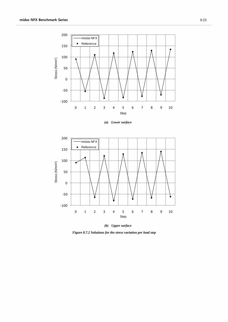
midas NFX Benchmark Series 8-23
(a) Lower surface
(b) Upper surface
Figure 8.7.2 Solutions for the stress variation per load step
-100
-50
0
50
100
150
200
0 1 2 3 4 5 6 7 8 9 10
Str
ess (N
/mm
2)
Step
midas NFX
Reference
-100
-50
0
50
100
150
200
0 1 2 3 4 5 6 7 8 9 10
Str
ess (N
/mm
2)
Step
midas NFX
Reference
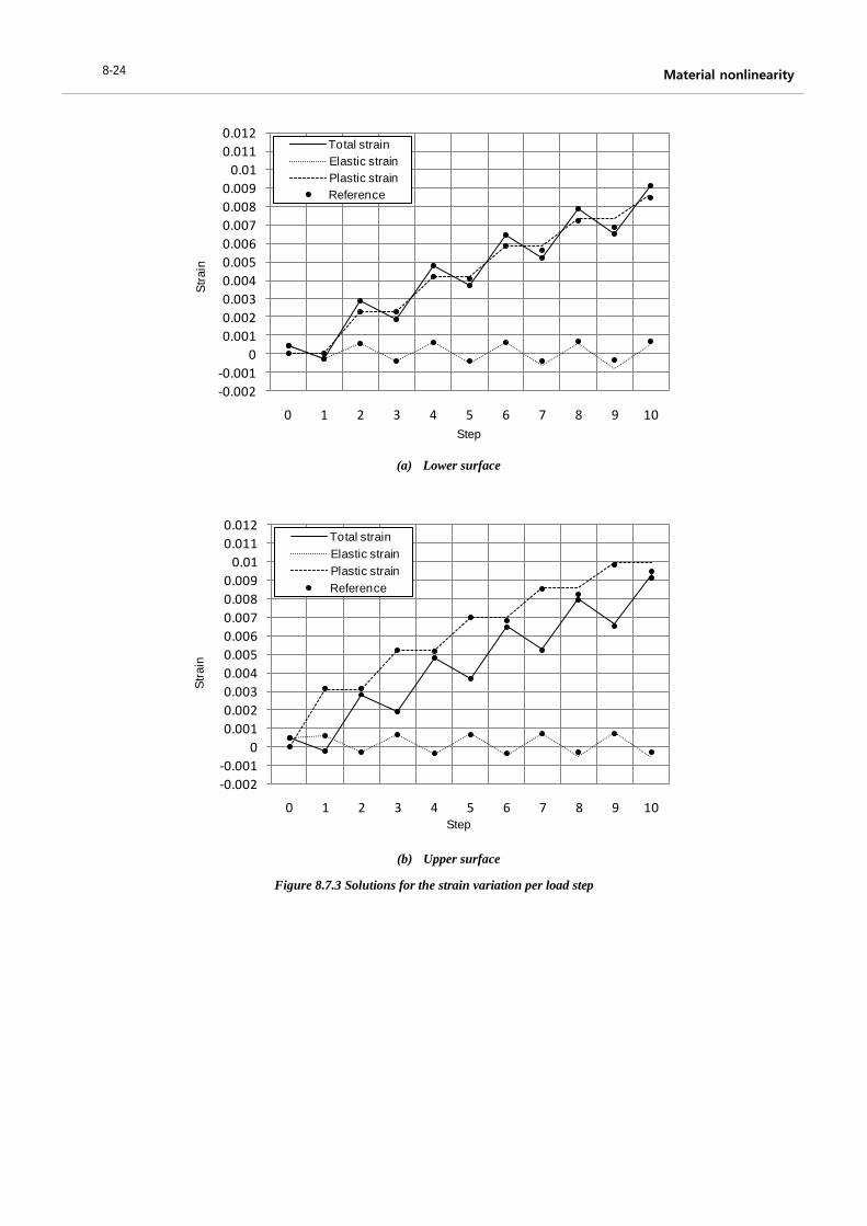
Material nonlinearity 8-24
(a) Lower surface
(b) Upper surface
Figure 8.7.3 Solutions for the strain variation per load step
-0.002
-0.001
0
0.001
0.002
0.003
0.004
0.005
0.006
0.007
0.008
0.009
0.01
0.011
0.012
0 1 2 3 4 5 6 7 8 9 10
Str
ain
Step
Total strain
Elastic strain
Plastic strain
Reference
-0.002
-0.001
0
0.001
0.002
0.003
0.004
0.005
0.006
0.007
0.008
0.009
0.01
0.011
0.012
0 1 2 3 4 5 6 7 8 9 10
Str
ain
Step
Total strain
Elastic strain
Plastic strain
Reference
25
midas NFX Benchmark Series 8-25
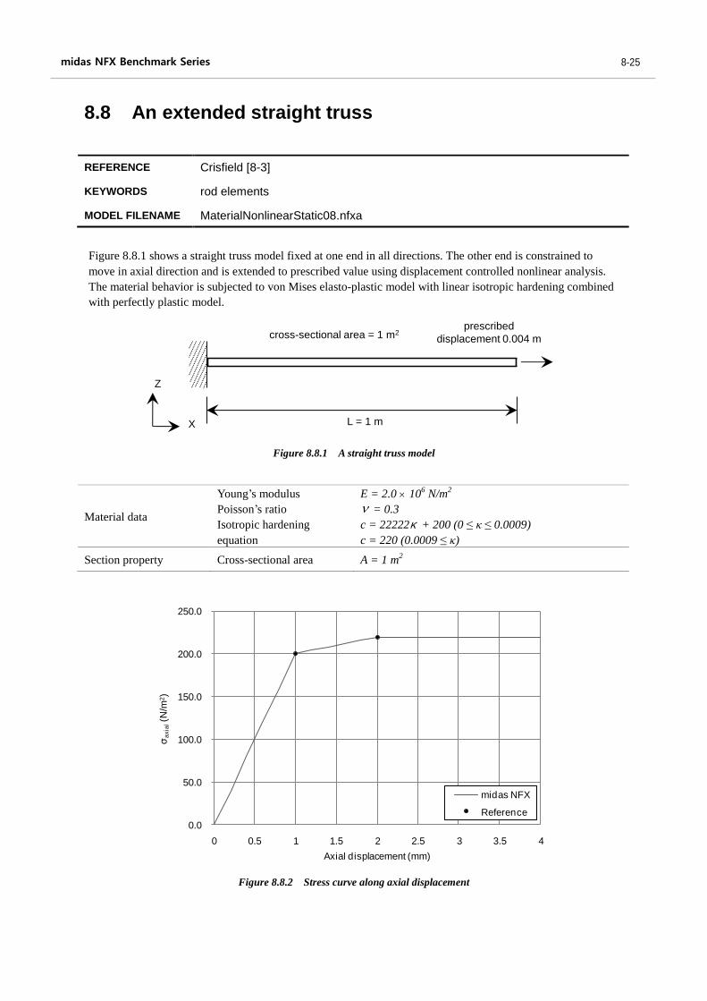
8.8 An extended straight truss
REFERENCE Crisfield [8-3]
KEYWORDS rod elements
MODEL FILENAME MaterialNonlinearStatic08.nfxa
Figure 8.8.1 A straight truss model
Material data
Young’s modulus
Poisson’s ratio
Isotropic hardening
equation
E = 2.0 106 N/m
2
= 0.3
c = 22222κ + 200 (0 ≤ κ ≤ 0.0009)
c = 220 (0.0009 ≤ κ)
Section property Cross-sectional area A = 1 m2
Figure 8.8.2 Stress curve along axial displacement
X
Z
L = 1 m
prescribed
displacement 0.004 mcross-sectional area = 1 m2
0.0
50.0
100.0
150.0
200.0
250.0
0 0.5 1 1.5 2 2.5 3 3.5 4
σa
xia
l(N
/m2)
Axial displacement (mm)
midas NFX
Reference
Figure 8.8.1 shows a straight truss model fixed at one end in all directions. The other end is constrained to
move in axial direction and is extended to prescribed value using displacement controlled nonlinear analysis.
The material behavior is subjected to von Mises elasto-plastic model with linear isotropic hardening combined
with perfectly plastic model.

Material nonlinearity 8-26
8.9 Square plate under uniformly distributed load
REFERENCE NAFEMS [8-2]
KEYWORDS shell elements
MODEL FILENAME MaterialNonlinearStatic09.nfxa
Figure 8.9.1 Square plate model
Material data
Young’s modulus
Poisson’s ratio
Perfect plasticity
E = 30000.0 N/mm2
= 0.3
Y = 30.0 N/mm2
Section property Thickness t = 0.4 mm
Table 8.9.1 Load per unit area for the plastic state
40
40
0.4Units: mm
Simply supported Clamped edge
limP [N/mm2] limP [N/mm
2]
Reference 0.01877 0.03852
QUAD-4 0.01880 0.03850
TRIA-3 0.01880 0.03850
QUAD-8 0.01880 0.03850
TRIA-6 0.01861 0.03850
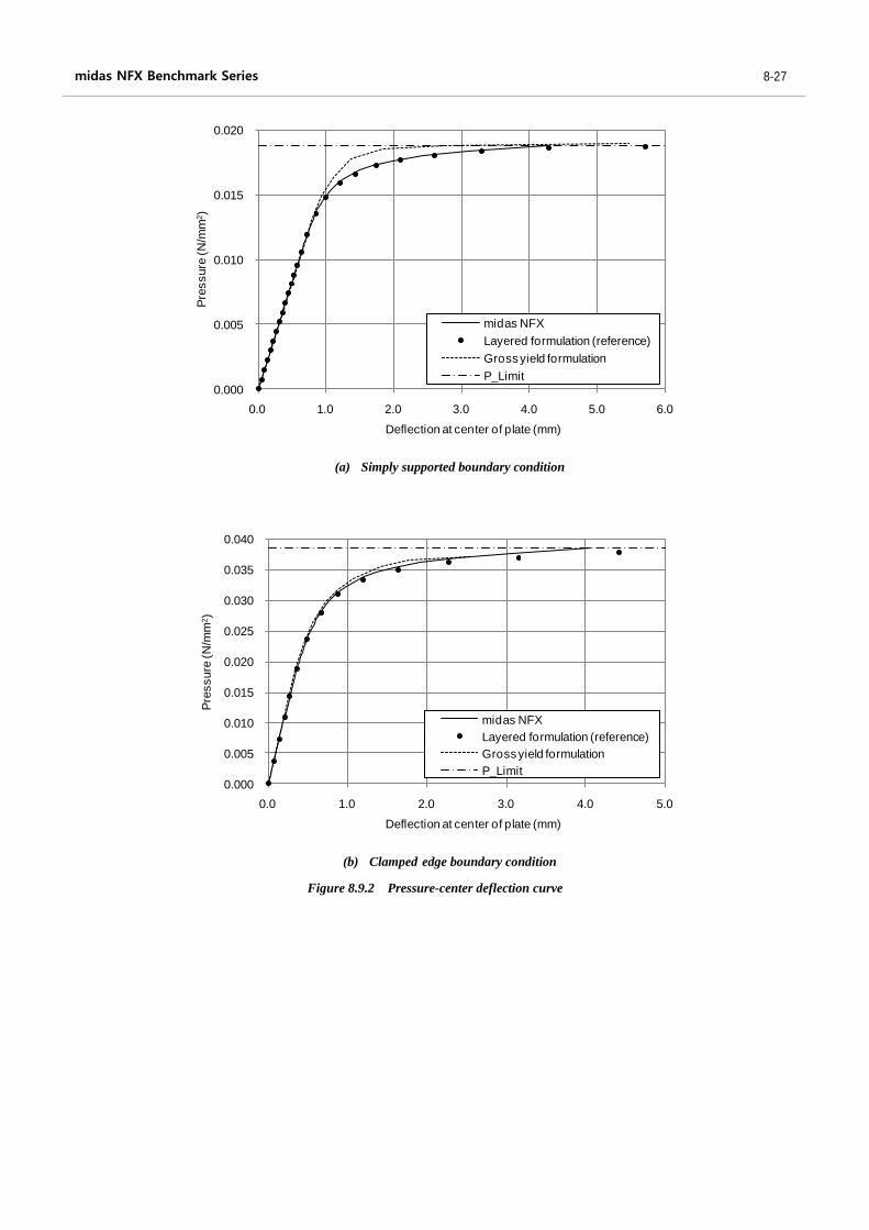
Figure 8.9.1 shows a square plate subjected to uniformly distributed load. The load is applied up to the yielding
point. The plate material follows the von Mises elastic perfectly plastic material model without hardening. The
shell section is integrated in the thickness direction using 13-point Simpson integration rule. Two boundary
edge conditions are tested: simply supported and clamped edge.
27
midas NFX Benchmark Series 8-27
(a) Simply supported boundary condition
(b) Clamped edge boundary condition
Figure 8.9.2 Pressure-center deflection curve
0.000
0.005
0.010
0.015
0.020
0.0 1.0 2.0 3.0 4.0 5.0 6.0
Pre
ssure
(N
/mm
2)
Deflection at center of plate (mm)
midas NFX
Layered formulation (reference)
Gross yield formulation
P_Limit
0.000
0.005
0.010
0.015
0.020
0.025
0.030
0.035
0.040
0.0 1.0 2.0 3.0 4.0 5.0
Pre
ssure
(N
/mm
2)
Deflection at center of plate (mm)
midas NFX
Layered formulation (reference)
Gross yield formulation
P_Limit
Material nonlinearity 8-28
8.10 Uniformly loaded circular plate
REFERENCE Owen et al. [8-4]
KEYWORDS axisymmetric elements
MODEL FILENAME MaterialNonlinearStatic10.nfxa
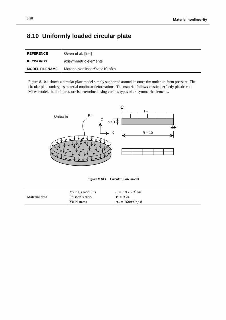
Figure 8.10.1 Circular plate model
Material data
Young’s modulus
Poisson’s ratio
Yield stress
E = 1.0 107 psi
= 0.24
Y = 16000.0 psi
PY
X
Z
PY
R = 10
h = 1
Units: in
C
Figure 8.10.1 shows a circular plate model simply supported around its outer rim under uniform pressure. The
circular plate undergoes material nonlinear deformations. The material follows elastic, perfectly plastic von
Mises model. the limit pressure is determined using various types of axisymmetric elements.
29
midas NFX Benchmark Series 8-29
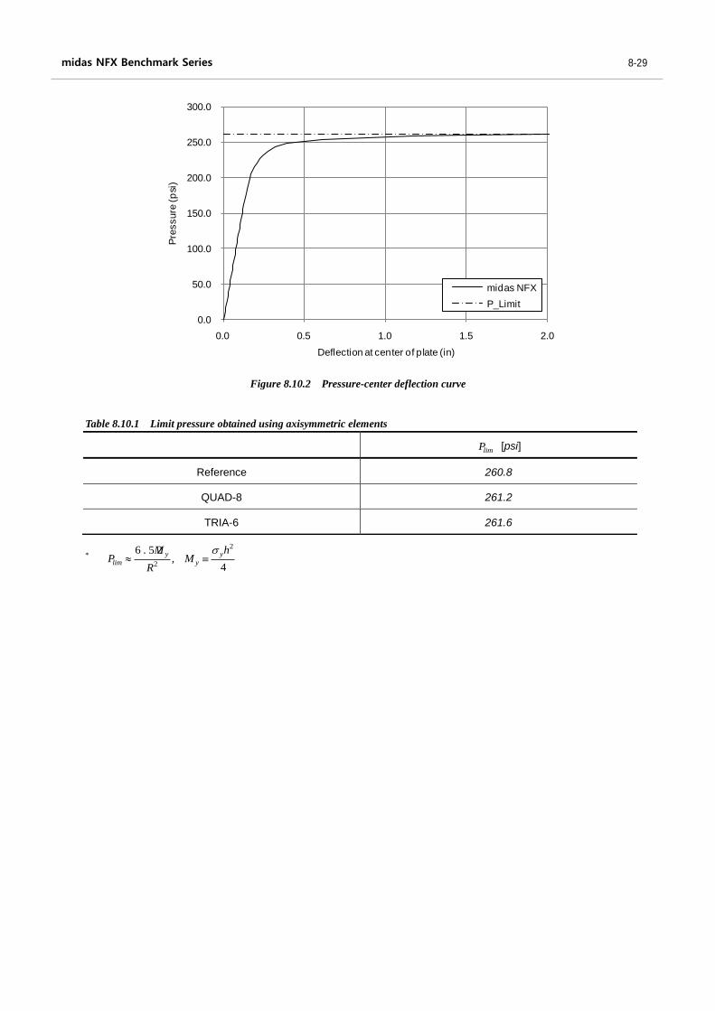
Figure 8.10.2 Pressure-center deflection curve
Table 8.10.1 Limit pressure obtained using axisymmetric elements
*
2
2
6 . 5 2,
4
y y
lim y
M hP M
R
0.0
50.0
100.0
150.0
200.0
250.0
300.0
0.0 0.5 1.0 1.5 2.0
Pre
ssure
(p
si)
Deflection at center of plate (in)
midas NFX
P_Limit
limP [psi]
Reference 260.8
QUAD-8 261.2
TRIA-6 261.6
Material nonlinearity 8-30
8.11 Two coaxial tubes
REFERENCE Crandall et al. [8-5]
KEYWORDS solid elements
MODEL FILENAME MaterialNonlinearStatic11.nfxa
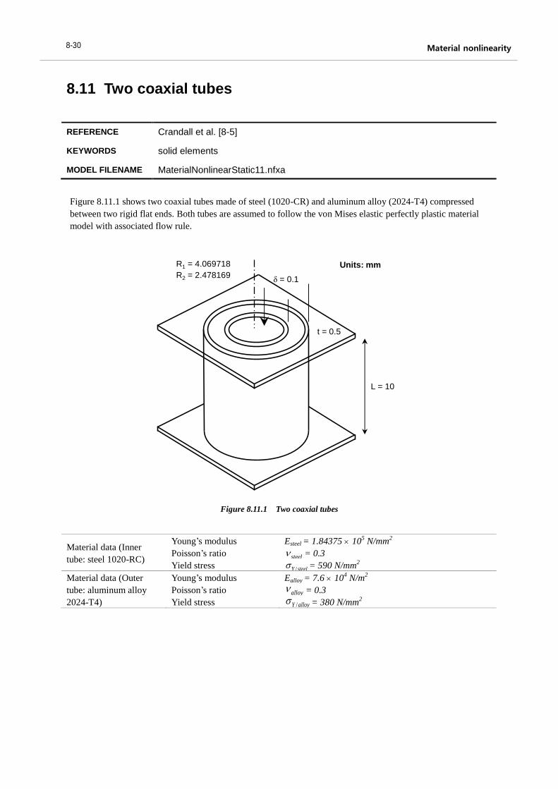
Figure 8.11.1 Two coaxial tubes
Material data (Inner
tube: steel 1020-RC)
Young’s modulus
Poisson’s ratio
Yield stress
Esteel = 1.84375 105 N/mm
2
steel = 0.3
/Y steel = 590 N/mm2
Material data (Outer
tube: aluminum alloy
2024-T4)
Young’s modulus
Poisson’s ratio
Yield stress
Ealloy = 7.6 104 N/m
2
alloy = 0.3
/Y alloy = 380 N/mm2
R1 = 4.069718
R2 = 2.478169
t = 0.5
Units: mm
δ = 0.1
L = 10
Figure 8.11.1 shows two coaxial tubes made of steel (1020-CR) and aluminum alloy (2024-T4) compressed
between two rigid flat ends. Both tubes are assumed to follow the von Mises elastic perfectly plastic material
model with associated flow rule.
31
midas NFX Benchmark Series 8-31
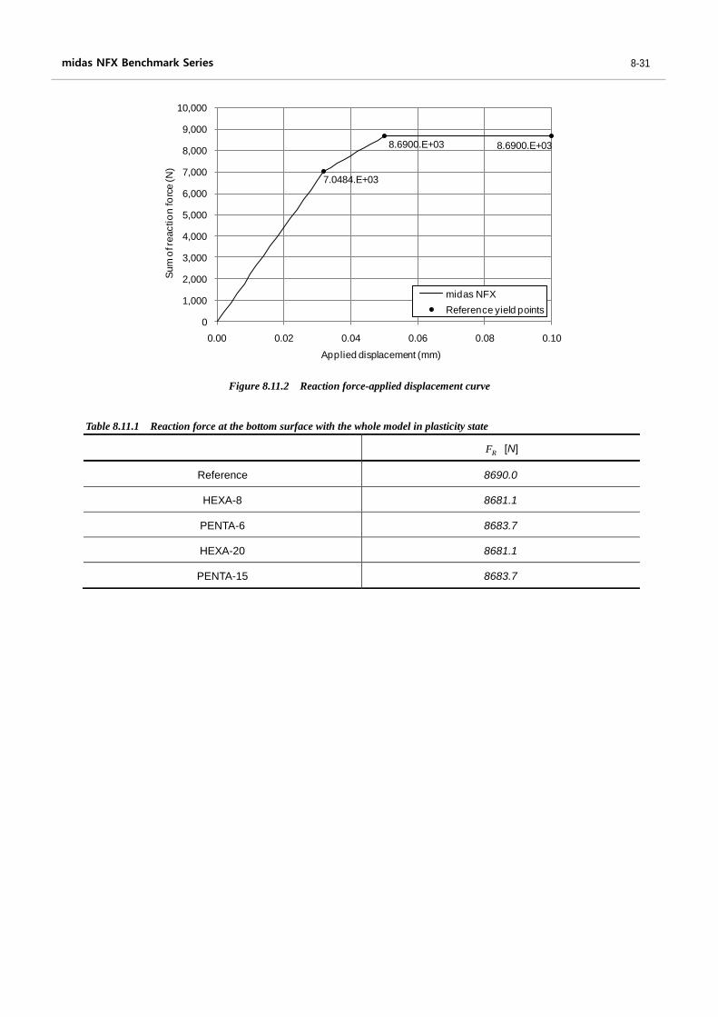
Figure 8.11.2 Reaction force-applied displacement curve
Table 8.11.1 Reaction force at the bottom surface with the whole model in plasticity state
7.0484.E+03
8.6900.E+03 8.6900.E+03
0
1,000
2,000
3,000
4,000
5,000
6,000
7,000
8,000
9,000
10,000
0.00 0.02 0.04 0.06 0.08 0.10
Sum
of r
eactio
n fo
rce (N
)
Applied displacement (mm)
midas NFX
Reference yield points
RF [N]
Reference 8690.0
HEXA-8 8681.1
PENTA-6 8683.7
HEXA-20 8681.1
PENTA-15 8683.7
Material nonlinearity 8-32
8.12 Residual stress problem
REFERENCE Crandall et al. [8-5]
KEYWORDS rod elements
MODEL FILENAME MaterialNonlinearStatic12.nfxa
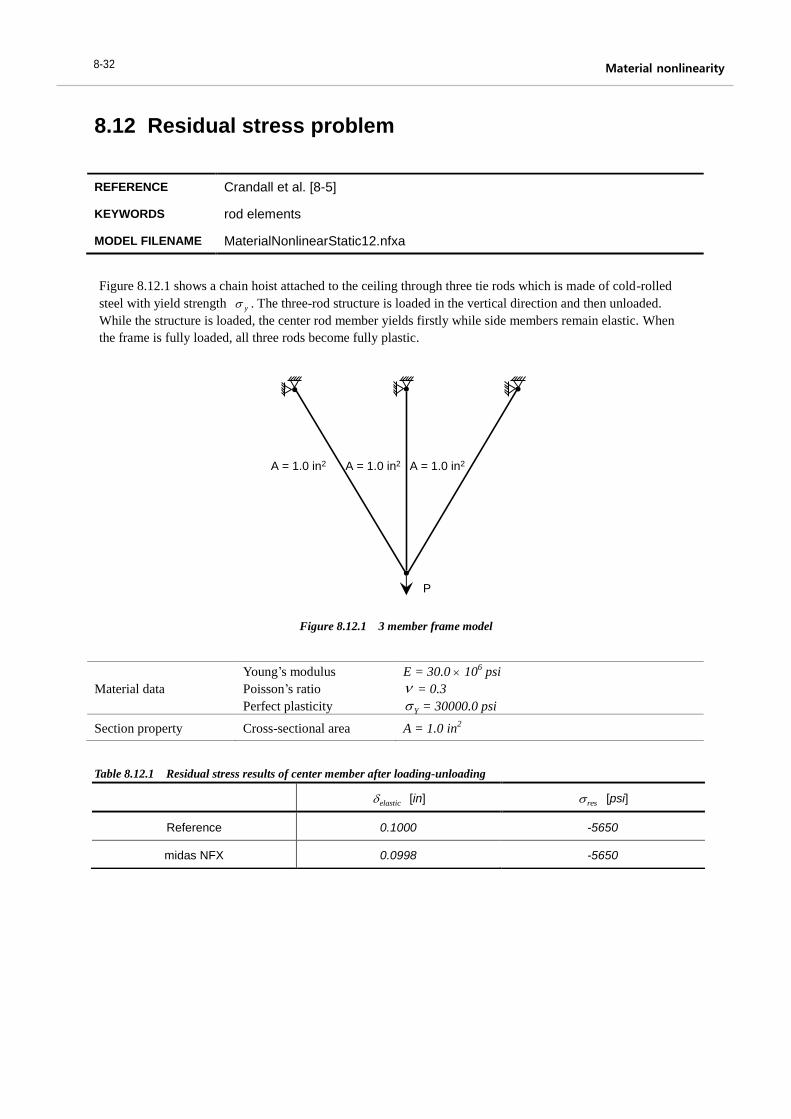
Figure 8.12.1 3 member frame model
Material data
Young’s modulus
Poisson’s ratio
Perfect plasticity
E = 30.0 106 psi
= 0.3
Y = 30000.0 psi
Section property Cross-sectional area A = 1.0 in2
Table 8.12.1 Residual stress results of center member after loading-unloading
A = 1.0 in2 A = 1.0 in2 A = 1.0 in2
P
elastic [in] res [psi]
Reference 0.1000 -5650
midas NFX 0.0998 -5650
Figure 8.12.1 shows a chain hoist attached to the ceiling through three tie rods which is made of cold-rolled
steel with yield strength y . The three-rod structure is loaded in the vertical direction and then unloaded.
While the structure is loaded, the center rod member yields firstly while side members remain elastic. When
the frame is fully loaded, all three rods become fully plastic.
33
midas NFX Benchmark Series 8-33
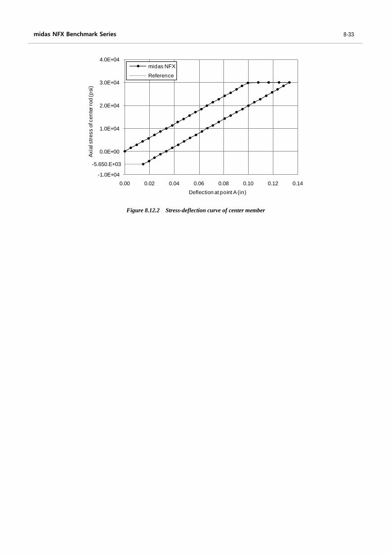
Figure 8.12.2 Stress-deflection curve of center member
-5.650.E+03
-1.0E+04
0.0E+00
1.0E+04
2.0E+04
3.0E+04
4.0E+04
0.00 0.02 0.04 0.06 0.08 0.10 0.12 0.14
Axia
l str
ess o
f cen
ter ro
d (p
si)
Deflection at point A (in)
midas NFX
Reference
Material nonlinearity 8-34
8.13 Nonlinear equation solution tests
REFERENCE NAFEMS [8-1]
KEYWORDS plane strain elements
MODEL FILENAME MaterialNonlinearStatic13.nfxa
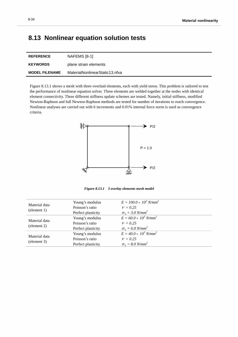
Figure 8.13.1 3 overlay elements mesh model
Material data
(element 1)
Young’s modulus
Poisson’s ratio
Perfect plasticity
E = 100.0 103 N/mm
2
= 0.25
Y = 3.0 N/mm2
Material data
(element 2)
Young’s modulus
Poisson’s ratio
Perfect plasticity
E = 60.0 103 N/mm
2
= 0.25
Y = 6.0 N/mm2
Material data
(element 3)
Young’s modulus
Poisson’s ratio
Perfect plasticity
E = 40.0 103 N/mm
2
= 0.25
Y = 8.0 N/mm2
P/2
P/2
P = 1.0
Figure 8.13.1 shows a mesh with three overlaid elements, each with yield stress. This problem is tailored to test
the performance of nonlinear equation solver. Three elements are welded together at the nodes with identical
element connectivity. Three different stiffness update schemes are tested. Namely, initial stiffness, modified
Newton-Raphson and full Newton-Raphson methods are tested for number of iterations to reach convergence.
Nonlinear analyses are carried out with 6 increments and 0.01% internal force norm is used as convergence
criteria.
35
midas NFX Benchmark Series 8-35
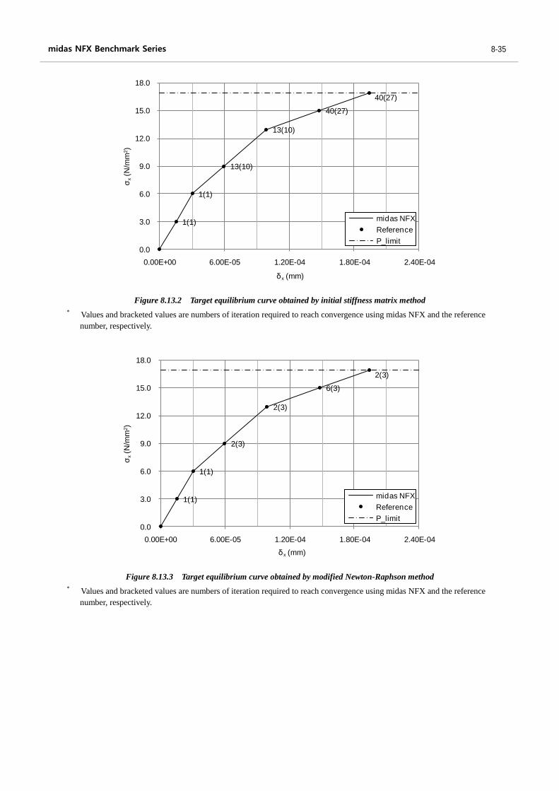
Figure 8.13.2 Target equilibrium curve obtained by initial stiffness matrix method
* Values and bracketed values are numbers of iteration required to reach convergence using midas NFX and the reference
number, respectively.
Figure 8.13.3 Target equilibrium curve obtained by modified Newton-Raphson method
* Values and bracketed values are numbers of iteration required to reach convergence using midas NFX and the reference
number, respectively.
1(1)
1(1)
13(10)
13(10)
40(27)
40(27)
0.0
3.0
6.0
9.0
12.0
15.0
18.0
0.00E+00 6.00E-05 1.20E-04 1.80E-04 2.40E-04
σx(N
/mm
2)
δx (mm)
midas NFX
Reference
P_limit
1(1)
1(1)
2(3)
2(3)
6(3)
2(3)
0.0
3.0
6.0
9.0
12.0
15.0
18.0
0.00E+00 6.00E-05 1.20E-04 1.80E-04 2.40E-04
σx(N
/mm
2)
δx (mm)
midas NFX
Reference
P_limit
Material nonlinearity 8-36
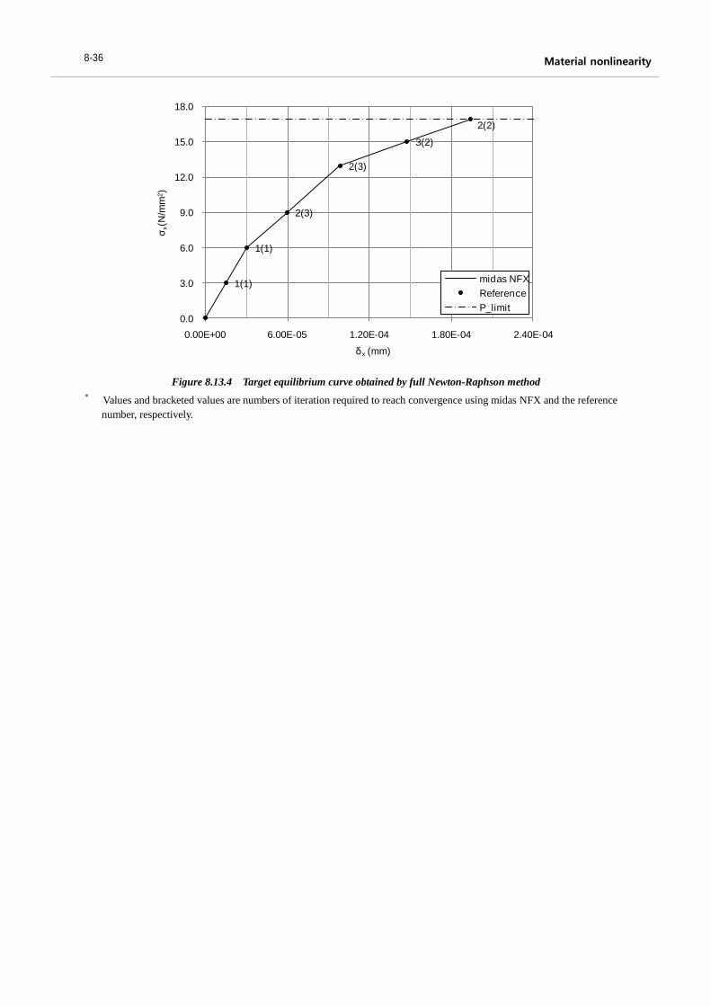
Figure 8.13.4 Target equilibrium curve obtained by full Newton-Raphson method
* Values and bracketed values are numbers of iteration required to reach convergence using midas NFX and the reference
number, respectively.
1(1)
1(1)
2(3)
2(3)
3(2)
2(2)
0.0
3.0
6.0
9.0
12.0
15.0
18.0
0.00E+00 6.00E-05 1.20E-04 1.80E-04 2.40E-04
σx(N
/mm
2)
δx (mm)
midas NFX
Reference
P_limit
37
midas NFX Benchmark Series 8-37
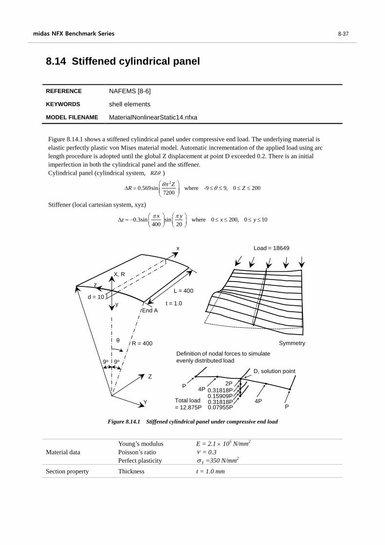
8.14 Stiffened cylindrical panel
REFERENCE NAFEMS [8-6]
KEYWORDS shell elements
MODEL FILENAME MaterialNonlinearStatic14.nfxa
Figure 8.14.1 Stiffened cylindrical panel under compressive end load
Material data
Young’s modulus
Poisson’s ratio
Perfect plasticity
E = 2.1 105 N/mm
2
= 0.3
Y =350 N/mm2
Section property Thickness t = 1.0 mm
End A
Y
Z
9o
L = 400d = 10
X, R
y
9o
θ
x
z
R = 400
t = 1.0
Load = 18649
Symmetry
Definition of nodal forces to simulate
evenly distributed load
Total load
= 12.875P P4P
P4P
2P
0.07955P0.31818P0.15909P0.31818P
D, solution point
Figure 8.14.1 shows a stiffened cylindrical panel under compressive end load. The underlying material is
elastic perfectly plastic von Mises material model. Automatic incrementation of the applied load using arc
length procedure is adopted until the global Z displacement at point D exceeded 0.2. There is an initial
imperfection in both the cylindrical panel and the stiffener.
Cylindrical panel (cylindrical system, RZ )
2
0.569sin where -9 9, 0 2007200
ZR Z
Stiffener (local cartesian system, xyz)
0.3sin sin where 0 200, 0 10400 20
x yz x y
Material nonlinearity 8-38
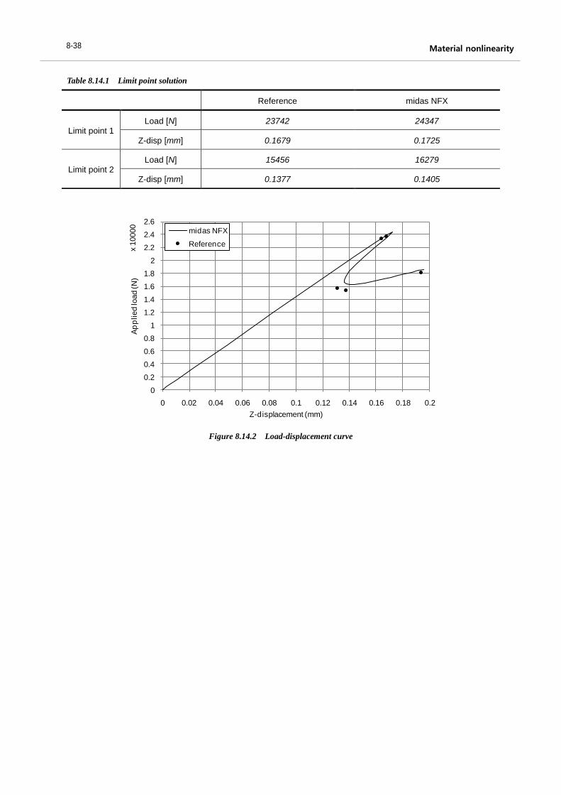
Table 8.14.1 Limit point solution
Figure 8.14.2 Load-displacement curve
0
0.2
0.4
0.6
0.8
1
1.2
1.4
1.6
1.8
2
2.2
2.4
2.6
0 0.02 0.04 0.06 0.08 0.1 0.12 0.14 0.16 0.18 0.2
Ap
plied lo
ad (N
)x 1
0000
Z-displacement (mm)
midas NFX
Reference
Reference midas NFX
Limit point 1 Load [N] 23742 24347
Z-disp [mm] 0.1679 0.1725
Limit point 2 Load [N] 15456 16279
Z-disp [mm] 0.1377 0.1405
39
midas NFX Benchmark Series 8-39
8.15 Necking of a circular bar
REFERENCE Simo et al. [8-7]
KEYWORDS axisymmetric elements, solid elements
MODEL FILENAME MaterialNonlinearStatic15.nfxa
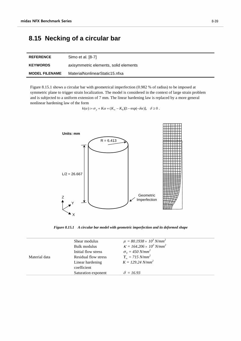
Figure 8.15.1 A circular bar model with geometric imperfection and its deformed shape
Material data
Shear modulus
Bulk modulus
Initial flow stress
Residual flow stress
Linear hardening
coefficient
Saturation exponent
= 80.1938 103 N/mm
2
= 164.206 103 N/mm
2
Y = 450 N/mm2
Y = 715 N/mm2
K = 129.24 N/mm2
= 16.93
X
Y
ZGeometric
Imperfection
R = 6.413
L/2 = 26.667
Units: mm
Figure 8.15.1 shows a circular bar with geometrical imperfection (0.982 % of radius) to be imposed at
symmetric plane to trigger strain localization. The model is considered in the context of large strain problem
and is subjected to a uniform extension of 7 mm. The linear hardening law is replaced by a more general
nonlinear hardening law of the form
0( ) : ( )[1 exp( )], 0yk K K K .
Material nonlinearity 8-40
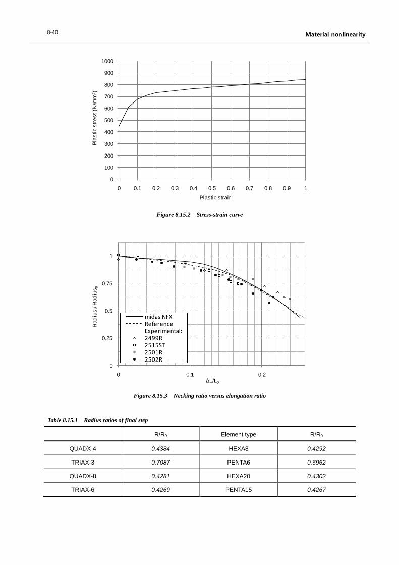
Figure 8.15.2 Stress-strain curve
Figure 8.15.3 Necking ratio versus elongation ratio
Table 8.15.1 Radius ratios of final step
0
100
200
300
400
500
600
700
800
900
1000
0 0.1 0.2 0.3 0.4 0.5 0.6 0.7 0.8 0.9 1
Pla
stic s
tress
(N
/mm
2)
Plastic strain
0
0.25
0.5
0.75
1
0 0.1 0.2
Rad
ius /
Rad
ius
0
ΔL/L0
midas NFXReferenceExperimental:2499R2515ST2501R2502R
R/R0 Element type R/R0
QUADX-4 0.4384 HEXA8 0.4292
TRIAX-3 0.7087 PENTA6 0.6962
QUADX-8 0.4281 HEXA20 0.4302
TRIAX-6 0.4269 PENTA15 0.4267
41
midas NFX Benchmark Series 8-41
8.16 Pressurized rubber disc
REFERENCE Oden [8-8]
KEYWORDS solid elements
MODEL FILENAME MaterialNonlinearStatic16.nfxa
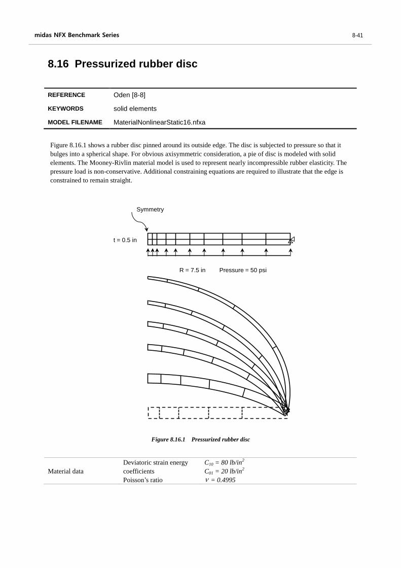
Figure 8.16.1 Pressurized rubber disc
Material data
Deviatoric strain energy
coefficients
Poisson’s ratio
C10 = 80 lb/in2
C01 = 20 lb/in2
= 0.4995
t = 0.5 in
Pressure = 50 psi
Symmetry
R = 7.5 in
Figure 8.16.1 shows a rubber disc pinned around its outside edge. The disc is subjected to pressure so that it
bulges into a spherical shape. For obvious axisymmetric consideration, a pie of disc is modeled with solid
elements. The Mooney-Rivlin material model is used to represent nearly incompressible rubber elasticity. The
pressure load is non-conservative. Additional constraining equations are required to illustrate that the edge is
constrained to remain straight.

Material nonlinearity 8-42
Figure 8.16.2 Thickness strain vs. central displacement
Figure 8.16.3 Pressure vs. deflection curve
0
0.1
0.2
0.3
0.4
0.5
0.6
0.7
0.8
0.9
1
0 0.5 1 1.5 2 2.5 3
Th
ickn
ess
/ Ori
gin
al t
hic
kness
Uz / R0
midas NFX
Reference
0
10
20
30
40
50
60
0 2 4 6 8 10 12 14 16 18 20
Pre
ssure
(p
si)
Uz (in)
midas NFX
Reference
43
midas NFX Benchmark Series 8-43
8.17 Inflation of a spherical rubber balloon
REFERENCE Souza et al. [8-9]
KEYWORDS solid elements
MODEL FILENAME MaterialNonlinearStatic17.nfxa
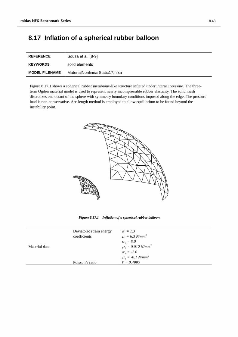
Figure 8.17.1 Inflation of a spherical rubber balloon
Material data
Deviatoric strain energy
coefficients
Poisson’s ratio
1 = 1.3
1 = 6.3 N/mm2
2 = 5.0
2 = 0.012 N/mm2
3 = -2.0
3 = -0.1 N/mm2
= 0.4995
Figure 8.17.1 shows a spherical rubber membrane-like structure inflated under internal pressure. The three-
term Ogden material model is used to represent nearly incompressible rubber elasticity. The solid mesh
discretizes one octant of the sphere with symmetry boundary conditions imposed along the edge. The pressure
load is non-conservative. Arc-length method is employed to allow equilibrium to be found beyond the
instability point.
Material nonlinearity 8-44
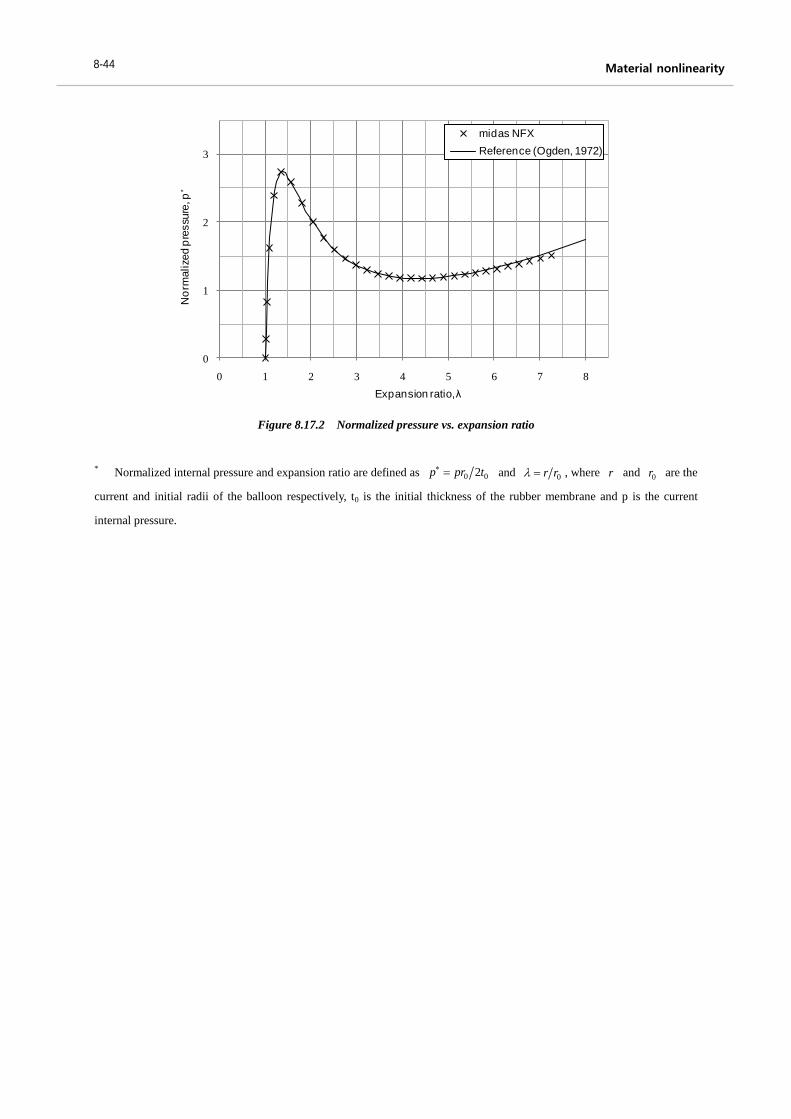
Figure 8.17.2 Normalized pressure vs. expansion ratio
* Normalized internal pressure and expansion ratio are defined as 0 02p pr t and 0r r , where r and 0r are the
current and initial radii of the balloon respectively, t0 is the initial thickness of the rubber membrane and p is the current
internal pressure.
0
1
2
3
0 1 2 3 4 5 6 7 8
No
rmalize
d p
ressu
re, p
*
Expansion ratio, λ
midas NFX
Reference (Ogden, 1972)
45
midas NFX Benchmark Series 8-45
8.18 Inflation of an axisymmetric ellipsoidal balloon
REFERENCE Souza et al. [8-9]
KEYWORDS solid elements
MODEL FILENAME MaterialNonlinearStatic18.nfxa
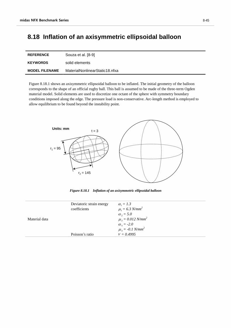
Figure 8.18.1 Inflation of an axisymmetric ellipsoidal balloon
Material data
Deviatoric strain energy
coefficients
Poisson’s ratio
1 = 1.3
1 = 6.3 N/mm2
2 = 5.0
2 = 0.012 N/mm2
3 = -2.0
3 = -0.1 N/mm2
= 0.4995
r2 = 145
r1 = 95
t = 3Units: mm
Figure 8.18.1 shows an axisymmetric ellipsoidal balloon to be inflated. The initial geometry of the balloon
corresponds to the shape of an official rugby ball. This ball is assumed to be made of the three-term Ogden
material model. Solid elements are used to discretize one octant of the sphere with symmetry boundary
conditions imposed along the edge. The pressure load is non-conservative. Arc-length method is employed to
allow equilibrium to be found beyond the instability point.
Material nonlinearity 8-46
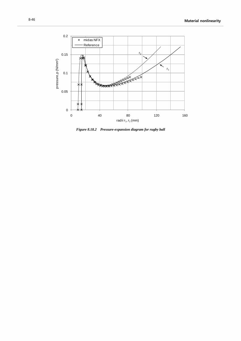
Figure 8.18.2 Pressure-expansion diagram for rugby ball
0
0.05
0.1
0.15
0.2
0 40 80 120 160
pre
ssure
, p (N
/mm
2)
radii r1, r2 (mm)
midas NFX
Reference
r2
r1
47
midas NFX Benchmark Series 8-47
8.19 Contact between a rigid body and a hyperelastic body
REFERENCE Zhi-Qiang Feng et al. [8-10]
KEYWORDS solid elements
MODEL FILENAME MaterialNonlinearStatic18.nfxa
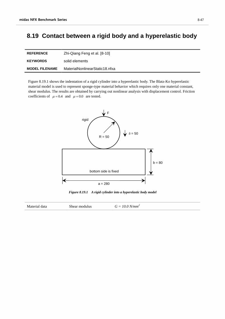
Figure 8.19.1 A rigid cylinder into a hyperelastic body model
Material data Shear modulus G = 10.0 N/mm2
R = 50
b = 80
a = 280
F
δ = 50
rigid
bottom side is fixed
Figure 8.19.1 shows the indentation of a rigid cylinder into a hyperelastic body. The Blatz-Ko hyperelastic
material model is used to represent sponge-type material behavior which requires only one material constant,
shear modulus. The results are obtained by carrying out nonlinear analysis with displacement control. Friction
coefficients of 0.4 and 0.0 are tested.

Material nonlinearity 8-48
Figure 8.19.2 Load-displacement curve
Figure 8.19.3 Deformed shape of the sponge type body (μ = 0.4)
0
1000
2000
3000
4000
5000
6000
7000
8000
9000
10000
0 10 20 30 40 50
Fo
rce (N
)
Displacement of the cylinder (mm)
midas NFX
Reference
μ= 0.4
μ= 0.0
49
midas NFX Benchmark Series 8-49
References
[8-1] NAFEMS, Background to material Non-Linear Benchmarks, Ref . R0049, NAFEMS, Glasgow, 1998
[8-2] NAFEMS, Selected Benchmarks for Material Non-Linearity, Ref . R0026, NAFEMS, Glasgow, 1993
[8-3] M. A. Crisfield, Non-linear Finite Element Analysis of Solids and Structures, England, John Wiley &
Sons Ltd., 1994
[8-4] D.R.J. Owen and E. Hinton, Finite elements in plasticity – Theory and Practice, Pineridge Press Limited,
Swansea, U.K., 1980
[8-5] S. H. Crandall and N. C. Dahl, An Introduction to the Mechanics of Solids, McGraw-Hill Book Co., Inc.,
New York, NY, 1959
[8-6] NAFEMS, A Review of Benchmark Problems for Geometric Non-linear Behaviour of 3-D Beams and
Shells, Ref . R0024, NAFEMS, Glasgow, 1993
[8-7] J. C. Simo, T. J. R. Hughes, Computational inelasticity, Springer-Verlag, New York, pp. 326-335 1998
[8-8] J. T. Oden, Finite elements of nonlinear continua, McGraw-Hill, 1972
[8-9] E. A. de Souza Neto, D. Peric and D. R. J. Owen, Computational Methods for plasticity, Wiley, New
York, 2008
[8-10] Zhi-Qiang Feng, Francois Peyraut, Nadia Labed, “Solution of large deformation contact problems with
friction between Blatz-Ko hyperelastic bodies,” International Journal of Engineering Science, Vol. 41, pp.
2213-2225, 2003