8 Hyperspectral Remote Sensing - University of Maryland ... · 8 Hyperspectral Remote Sensing Eyal...
44
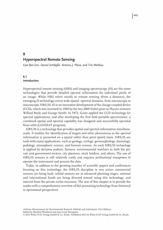
413 8 Hyperspectral Remote Sensing Eyal Ben-Dor, Daniel Schl¨ apfer, Antonio J. Plaza, and Tim Malthus 8.1 Introduction Hyperspectral remote sensing (HRS) and imaging spectroscopy (IS) are the same technologies that provide detailed spectral information for individual pixels of an image. While HRS refers mostly to remote sensing (from a distance), the emerging IS technology covers wide spatial – spectral domains, from microscopic to macroscopic HRS/IS. IS is an innovative development of the charge-coupled device (CCD), which was invented in 1969 by the two 2009 Nobel prize in Physics winners Willard Boyle and George Smith. In 1972, Goetz applied the CCD technology for spectral applications, and after developing the first field portable spectrometer, a combined spatial and spectral capability was designed and successfully operated from orbit (LANDSAT program). HRS/IS is a technology that provides spatial and spectral information simultane- ously. It enables the identification of targets and other phenomena as the spectral information is presented on a spatial rather than point (pixel) basis. HRS/IS are tools with many applications, such as geology, ecology, geomorphology, limnology, pedology, atmospheric science, and forensic science. As such HRS/IS technology is applied by decision makers, farmers, environmental watchers in both the pri- vate and government sectors, city planners, stock holders, and others. The use of HRS/IS sensors is still relatively costly and requires professional manpower to operate the instrument and process the data. Today, in addition to the growing number of scientific papers and conferences focusing on this technology, the HRS/IS discipline is very active: commercial sensors are being built, orbital sensors are in advanced planning stages, national and international funds are being directed toward using this technology, and interest from the private sector increases. The aim of this chapter is to provide the reader with a comprehensive overview of this promising technology from historical to operational perspectives. Airborne Measurements for Environmental Research: Methods and Instruments, First Edition. Edited by Manfred Wendisch and Jean-Louis Brenguier. © 2013 Wiley-VCH Verlag GmbH & Co. KGaA. Published 2013 by Wiley-VCH Verlag GmbH & Co. KGaA.
Transcript of 8 Hyperspectral Remote Sensing - University of Maryland ... · 8 Hyperspectral Remote Sensing Eyal...
413
8Hyperspectral Remote SensingEyal Ben-Dor, Daniel Schlapfer, Antonio J. Plaza, and Tim Malthus
8.1Introduction
Hyperspectral remote sensing (HRS) and imaging spectroscopy (IS) are the sametechnologies that provide detailed spectral information for individual pixels ofan image. While HRS refers mostly to remote sensing (from a distance), theemerging IS technology covers wide spatial–spectral domains, from microscopic tomacroscopic HRS/IS. IS is an innovative development of the charge-coupled device(CCD), which was invented in 1969 by the two 2009 Nobel prize in Physics winnersWillard Boyle and George Smith. In 1972, Goetz applied the CCD technology forspectral applications, and after developing the first field portable spectrometer, acombined spatial and spectral capability was designed and successfully operatedfrom orbit (LANDSAT program).
HRS/IS is a technology that provides spatial and spectral information simultane-ously. It enables the identification of targets and other phenomena as the spectralinformation is presented on a spatial rather than point (pixel) basis. HRS/IS aretools with many applications, such as geology, ecology, geomorphology, limnology,pedology, atmospheric science, and forensic science. As such HRS/IS technologyis applied by decision makers, farmers, environmental watchers in both the pri-vate and government sectors, city planners, stock holders, and others. The use ofHRS/IS sensors is still relatively costly and requires professional manpower tooperate the instrument and process the data.
Today, in addition to the growing number of scientific papers and conferencesfocusing on this technology, the HRS/IS discipline is very active: commercialsensors are being built, orbital sensors are in advanced planning stages, nationaland international funds are being directed toward using this technology, andinterest from the private sector increases. The aim of this chapter is to provide thereader with a comprehensive overview of this promising technology from historicalto operational perspectives.
Airborne Measurements for Environmental Research: Methods and Instruments, First Edition.Edited by Manfred Wendisch and Jean-Louis Brenguier.© 2013 Wiley-VCH Verlag GmbH & Co. KGaA. Published 2013 by Wiley-VCH Verlag GmbH & Co. KGaA.
414 8 Hyperspectral Remote Sensing
8.2Definition
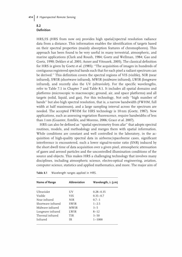
HRS/IS (HRS from now on) provides high spatial/spectral resolution radiancedata from a distance. This information enables the identification of targets basedon their spectral properties (mainly absorption features of chromophores). Thisapproach has been found to be very useful in many terrestrial, atmospheric, andmarine applications (Clark and Roush, 1984; Goetz and Wellman, 1984; Gao andGoetz, 1990; Dekker et al. 2001; Asner and Vitousek, 2005). The classical definitionfor HRS is given by Goetz et al. (1985): ‘‘The acquisition of images in hundreds ofcontiguous registered spectral bands such that for each pixel a radiant spectrum canbe derived.’’ This definition covers the spectral regions of VIS (visible), NIR (nearinfrared), SWIR (shortwave infrared), MWIR (midwave infrared), LWIR (longwaveinfrared), and recently also the UV (ultraviolet). For the specific wavelengths,refer to Table 7.1 in Chapter 7 and Table 8.1. It includes all spatial domains andplatforms (microscopic to macroscopic; ground, air, and space platforms) and alltargets (solid, liquid, and gas). For this technology, Not only ‘‘high number ofbands’’ but also high spectral resolution, that is, a narrow bandwidth (FWHM, fullwidth at half maximum), and a large sampling interval across the spectrum areneeded. The accepted FWHM for HRS technology is 10 nm (Goetz, 1987). Newapplications, such as assessing vegetation fluorescence, require bandwidths of lessthan 1 nm (Guanter, Estelles, and Moreno, 2006; Grace et al. 2007).
HRS can also be defined as ‘‘spatial spectrometry from afar’’ that adopts spectralroutines, models, and methodology and merges them with spatial information.While conditions are constant and well controlled in the laboratory, in the ac-quisition of high-quality spectral data in airborne/spaceborne cases, significantinterference is encountered, such a lower signal-to-noise ratio (SNR) induced bythe short dwell time of data acquisition over a given pixel, atmospheric attenuationof gases and aerosol particles and the uncontrolled illumination conditions of thesource and objects. This makes HRS a challenging technology that involves manydisciplines, including atmospheric science, electro-optical engineering, aviation,computer science, statistics and applied mathematics, and more. The major aim of
Table 8.1 Wavelength ranges applied in HRS.
Name of Range Abbreviation Wavelength, λ (μm)
Ultraviolet UV 0.28–0.35Visible VIS 0.35–0.7Near infrared NIR 0.7–1Shortwave infrared SWIR 1–2.5Midwave infrared MWIR 3–5Longwave infrared LWIR 8–12Thermal infrared TIR 3–50Infrared IR 1–1000
8.2 Definition 415
HRS is to extract physical information across the spectrum (radiance) to describe in-herent properties of the targets, such as reflectance and emissivity. Under laboratoryconditions, the spectral information across the UV-VIS-NIR-SWIR-MWIR-LWIRspectral regions can be quantitatively analyzed for a wealth of materials, natural andartificial, such as vegetation, water, gases, artificial material, soils, and rocks, withmany already available in spectral libraries. If a HRS sensor with high SNR is used,an analytical spectral approach yields new products (Clark, Gallagher, and Swayze,1990; Kruger, Erzinger, and Kaufmann, 1998). The high spectral resolution of HRStechnology combined with temporal coverage enables better recognition of targetsand an improved quantitative analysis of phenomena, especially for land use coverapplication.
Allocating spectral information temporally in a spatial domain provides a newdimension that neither the traditional point spectroscopy nor air photographycan provide separately. HRS can thus be described as an ‘‘expert’’ geographicinformation system (GIS) in which surface layers are built on a pixel-by-pixelbasis rather than a selected group of points with direct and indirect chemical andphysical information. Spatial recognition of the phenomenon in question is betterperformed in the HRS domain than by traditional GIS techniques. HRS consists ofmany points (actually the number of pixels in the image) that are used to generatethematic layers, whereas in GIS, only a few points are used to describe an area ofinterest (raster vs vector).
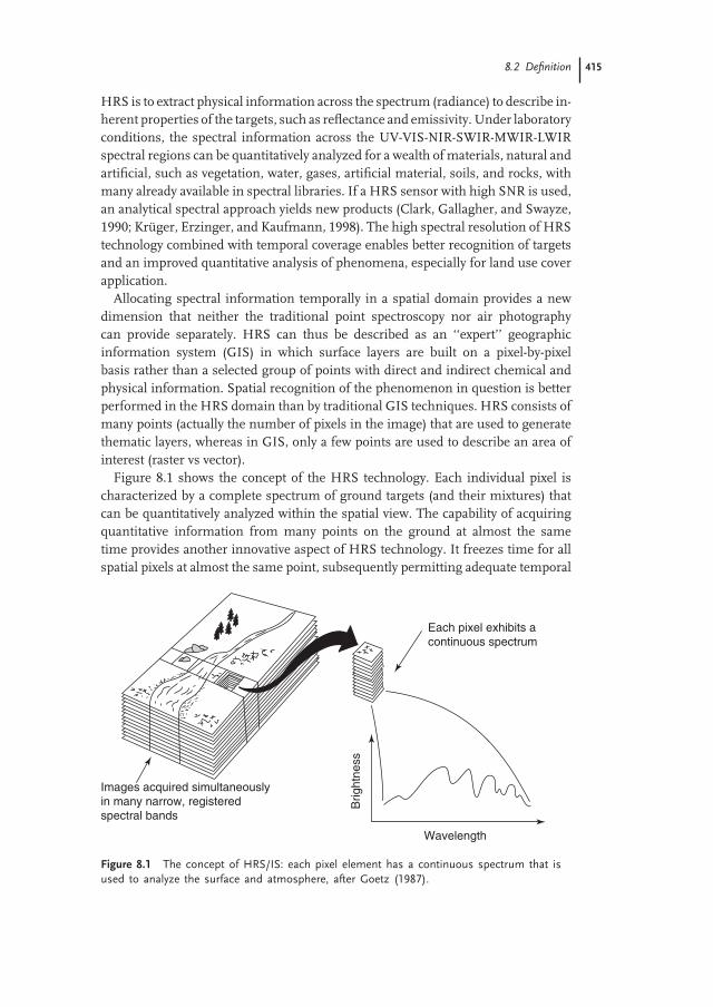
Figure 8.1 shows the concept of the HRS technology. Each individual pixel ischaracterized by a complete spectrum of ground targets (and their mixtures) thatcan be quantitatively analyzed within the spatial view. The capability of acquiringquantitative information from many points on the ground at almost the sametime provides another innovative aspect of HRS technology. It freezes time for allspatial pixels at almost the same point, subsequently permitting adequate temporal
Images acquired simultaneouslyin many narrow, registeredspectral bands
Each pixel exhibits acontinuous spectrum
Wavelength
Brig
htne
ss
Figure 8.1 The concept of HRS/IS: each pixel element has a continuous spectrum that isused to analyze the surface and atmosphere, after Goetz (1987).

416 8 Hyperspectral Remote Sensing
analysis. HRS technology is thus a promising tool that adds many new aspectsto the existing mapping technology and improves our capability to remote-sensematerials from far distances.
8.3History
Alex Goetz is considered a mentor and pioneer scientist in HRS technologytogether with his colleague Gregg Vane. Goetz (2009) and MacDonald, Ustin,and Schaepman (2009) reviewed the history of HRS development since 1970.HRS technology was driven by geologists and geophysicists who realized that theEarth’s surface mineralogy consists of significant and unique spectral fingerprintsacross the SWIR, MWR, and LWIR spectral regions (later the VIS–NIR spectralregion was also explored). This knowledge was gained from comprehensive workwith laboratory spectrometers and was followed by a physical explanation of thereflectance spectral response of minerals in rocks and soil. Hunt and Salisbury(1970, 1971); Hunt, Salisbury, and Lenhoff (1971a,b); Stoner and Baumgardner(1981); Clark (1999) created the first collection of available soil and rock spectrallibraries.
HRS capability leans heavily on the invention of the CCD assembly in 1969(Smith, 2001), which provided the first step toward digital imaging. These achieve-ments acted as a precursor to establishing a real image spectrometer that wouldrely on the commercial hybrid focal plane array that was available at that time (in1979). The first sensor of this kind was used in the shuttle mission SMIRR (shuttlemultispectral infrared radiometer) in 1981. In 1983, Goetz and Vane started tobuild an airborne HRS sensor (airborne imaging spectrometer, AIS), which wassensitive in the SWIR region (Goetz, 2009).
The 2D detector arrays (32 × 32 elements) consisted of HgCdTe detectorsgenerated images at wavelength greater than 1.1 μm. The array detector did notneed a scan and provided sufficient improvement in the SNR to suit airborneapplications. The AIS was a rather large instrument and was flown onboard aC-130 aircraft. It had two versions, with two modes being used in each: the ‘‘treemode’’ from 0.9 to 2.1 μm and the ‘‘rock mode’’ from 1.2 to 2.4 μm.
The instantaneous field of view (IFOV) of the AIS-1 was 1.91 mrad and of theAIS-2 2.05 mrad; the ground instantaneous field of view (GIFOV) (from 6 km) was11.4 and 12.3 m, and the FOV was 3.7◦ and 7.3◦, respectively. The image swath was365 m for AIS-1 and 787 m for AIS-2, with a spectral sampling interval of 9.3 and10.6 nm, respectively. The AIS-1 was flown from 1982 to 1985 and the AIS-2, a laterversion with spectral coverage of 0.8–2.4 μm and 64-pixel width (Vane and Goetz,1988), was operated in 1986. In those days, methods to account for atmosphericattenuation were not available; nonetheless, by simple approximation, the sensorand the HRS concept were able to show that minerals can be identified and spatiallymapped over an arid-environment terrain. The proceedings of a conference thatsummarized the activity and first results of the AIS missions were published by
8.4 Sensor Principles 417
the National Aeronautics and Space Administration (NASA) in 1985 and 1986.At that time, spectral libraries of mineral and rock material had not yet beendeveloped. Rowan proved that the HRS technology was able to detect the mineralbuddingtonite from afar and solved the mystery of unrecognized spectral featureat that time.
In 1984, Vane started to build AVIRIS (Airborne Visible and Infrared ImagingSpectrometer). The first developed AVIRIS lasted three years (1984–1987), withits first flight taking place in 1987. Although being a relatively low-quality SNRinstrument, the first AVIRIS demonstrated excellent performance relative to theAIS. The sensor covered the entire VIS-NIR-SWIR region with 224 bands (around10 nm FWHM), with 20 m GIFOV and around 10 × 10 km swath. It was a whiskb-room sensor with a SNR of around 100 carried onboard an ER-2 aircraft from20 km altitude. Since then, the AVIRIS sensor has undergone upgrades. The majordifferences are its SNR (100 in 1987 relative to >1000 today), spectral coverage(400–2500 nm vs 350–2500 nm today) and spatial resolution (20 m vs 2 m today).
The instrument can fly on different platforms at lower altitudes and has openedup new capabilities for potential users in many applications. Even today, with manynew HRS sensors having become available worldwide, the AVIRIS sensor is stillconsidered the best HSR sensor (Goetz, 2009). This is due in large part to carefulmaintenance and upgrade of the sensor over the years and to the growing interestof the HRS community in using the data. The AVIRIS program has established anactive HRS community in the United States and then in Europe that has rapidlymatured. On the basis of this capability and success, other sensors have beendeveloped and built over the past two decades worldwide.
8.4Sensor Principles
Imaging spectrometers typically use a two-dimensional (2D) matrix array (e.g., aCCD or focal plane array (FPA) that produces a 3D data cube (spatial dimensionsand a third spectral axis). These data cubes are built in a progressive manner by(i) sequentially recording one full spatial image after another, each at a differentwavelength, or (ii) sequentially recording one narrow image (1 pixel wide, multiplepixels long) swath after another with the corresponding spectral signature for eachpixel in the swath. Some common techniques used in airborne or spaceborneapplications are depicted in Figure 8.2. The first two approaches shown are basicones, used to generate images such as those used in LANDSAT (Figure 8.2a) andSPOT (Figure 8.2b). They show the concept of measuring reflected radiation in adiscrete detector or in a line array.
Multichannel sensors such as LANDSAT TM are optical mechanical system inwhich discrete, fixed detector elements are scanned across the target perpendicularto the flight path by a mirror and these detectors convert the reflected solar photonsfrom each pixel in the scene into an electronic signal. The detector elements areplaced behind filters that pass broad portions of the spectrum. One approach to
418 8 Hyperspectral Remote Sensing
Dispersing element
Slit
CollimatorLens
Objective
Areaarrays
Discretedetectors Lens
Foldmirror
(a)
(c) (d)
(b)
Scan mirror
Dispersing element
Linearray Objective
Entrance aperture
Collimator
Line array
Objective
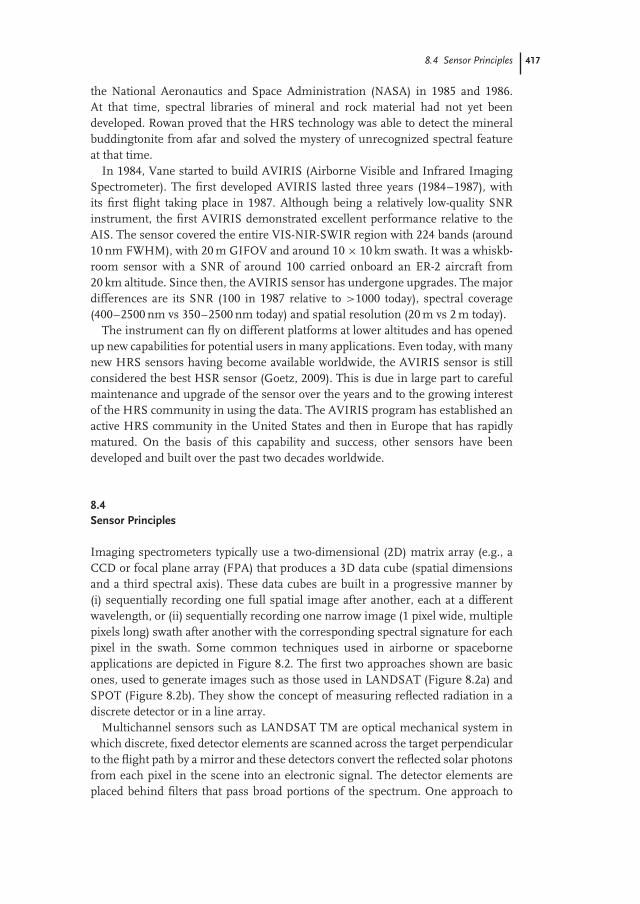
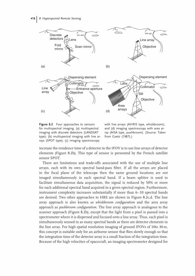
Figure 8.2 Four approaches to sensorsfor multispectral imaging. (a) multispectralimaging with discrete detectors (LANDSATtype); (b) multispectral imaging with line ar-rays (SPOT type); (c) imaging spectroscopy
with line arrays (AVIRIS type, whiskbroom);and (d) imaging spectroscopy with area ar-ray (AISA type, pushbroom). (Source: Takenfrom Goetz (1987).)
increase the residence time of a detector in the IFOV is to use line arrays of detectorelements (Figure 8.2b). This type of sensor is presented by the French satellitesensor SPOT.
There are limitations and trade-offs associated with the use of multiple linearrays, each with its own spectral band-pass filter. If all the arrays are placedin the focal plane of the telescope then the same ground locations are notimaged simultaneously in each spectral band. If a beam splitter is used tofacilitate simultaneous data acquisition, the signal is reduced by 50% or morefor each additional spectral band acquired in a given spectral region. Furthermore,instrument complexity increases substantially if more than 6–10 spectral bandsare desired. Two other approaches to HRS are shown in Figure 8.2c,d. The linearray approach is also known as whiskbroom configuration and the area arrayapproach as pushbroom configuration. The line array approach is analogous to thescanner approach (Figure 8.2b), except that the light from a pixel is passed into aspectrometer where it is dispersed and focused onto a line array. Thus, each pixel issimultaneously sensed in as many spectral bands as there are detector elements inthe line array. For high spatial resolution imaging of ground IFOVs of 10to 30 m,this concept is suitable only for an airborne sensor that flies slowly enough so thatthe integration time of the detector array is a small fraction of the integration time.Because of the high velocities of spacecraft, an imaging spectrometer designed for
8.5 HRS Sensors 419
the Earth’s orbit requires the use of two distinguished area arrays of the detector inthe focal plane of the spectrometer (Figure 8.2d), thereby obviating the need for anoptical scanning mechanism (pushbroom configuration).
The key to HRS is the detector array. Line arrays of silicon, sensitive to radiationat wavelengths of up to 1.1 μm, are available commercially in dimensions of upto 5000 elements in length. Area arrays of up to 800 × 800 elements of siliconwere developed for wide-field and planetary camera. However, the state of infraredarray development for wavelength beyond 1.1 μm is not so advanced. Line arraysare available in several materials up to few hindered detector elements in length.Two of the most attractive materials are mercury-cadmium-telluride (HgCdTe)and indium antimonite (InSb). InSb arrays of 512 elements with very highquantum efficiency and detectors with similar element-to-element responsivitieshave developed. The InSb arrays respond to wavelengths from 0.7 to 5.2 μm. Acomprehensive description of both pushbroom and whiskbroom technologies withadvantages and disadvantages can be found in Sellar and Boreman (2005).
8.5HRS Sensors
8.5.1General
The growing number of researchers in the HRS community can be seen by theirattendance at the yearly proceedings of the AVIRIS Workshop Series, organized byJPL since 1985 (starting with AIS, and today with HyspIRI) and other workshopsorganized by international groups such as WHISPERS (Work group on Hyper-spectral Image and Signal Processing: Evaluation in Remote Sensing) and EARSELSIG IS (European Remote Sensing Laboratory Special Interest Group on ImagingSpectroscopy). In 1993, a special issue of Remote Sensing of Environment was pub-lished, dedicated to HRS technology in general and to AVIRIS in particular (Vane,1993). This broadened the horizon for many potential users who still had not heardabout HRS technology, ensuring that the activity would continue. Today, new HRSprograms are up and running at NASA, such as the M3 (Moon Mineralogy Mapper)project in collaboration with the Indian Space Agency to study the moon’s surface(Pieters et al. 2009b), along with preparations to place a combined optical and ther-mal hyperspectral sensor in orbit, the HyspIRI (Hyperspectral Infrared Imager)project (Knox et al. 2010). In addition to the AIS and AVIRIS missions, NASA alsosuccessfully operated a thermal hyperspectral mission known as TIMS (thermalinfrared multispectral scanner) in circa 1980–1983 (Kahle and Goetz, 1983) andalso collaborated on other HRS initiatives in North America. The TIMS and, thenlater, the ASTER spacecraft sensors showed the thermal region’s promising capa-bility for obtaining mineral-based information. Apparently, the thermal infrared(TIR) HRS capability because of its costs and performance was set aside, and ithas only recently begun to garner new attention, in new space initiatives (HyspIRI)
420 8 Hyperspectral Remote Sensing
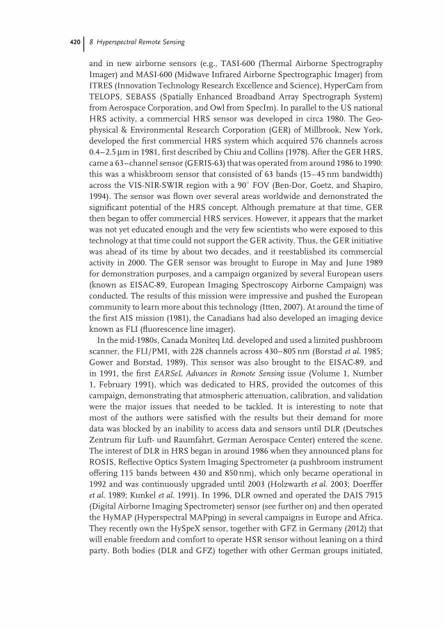
and in new airborne sensors (e.g., TASI-600 (Thermal Airborne SpectrographyImager) and MASI-600 (Midwave Infrared Airborne Spectrographic Imager) fromITRES (Innovation Technology Research Excellence and Science), HyperCam fromTELOPS, SEBASS (Spatially Enhanced Broadband Array Spectrograph System)from Aerospace Corporation, and Owl from SpecIm). In parallel to the US nationalHRS activity, a commercial HRS sensor was developed in circa 1980. The Geo-physical & Environmental Research Corporation (GER) of Millbrook, New York,developed the first commercial HRS system which acquired 576 channels across0.4–2.5 μm in 1981, first described by Chiu and Collins (1978). After the GER HRS,came a 63–channel sensor (GERIS-63) that was operated from around 1986 to 1990:this was a whiskbroom sensor that consisted of 63 bands (15–45 nm bandwidth)across the VIS-NIR-SWIR region with a 90◦ FOV (Ben-Dor, Goetz, and Shapiro,1994). The sensor was flown over several areas worldwide and demonstrated thesignificant potential of the HRS concept. Although premature at that time, GERthen began to offer commercial HRS services. However, it appears that the marketwas not yet educated enough and the very few scientists who were exposed to thistechnology at that time could not support the GER activity. Thus, the GER initiativewas ahead of its time by about two decades, and it reestablished its commercialactivity in 2000. The GER sensor was brought to Europe in May and June 1989for demonstration purposes, and a campaign organized by several European users(known as EISAC-89, European Imaging Spectroscopy Airborne Campaign) wasconducted. The results of this mission were impressive and pushed the Europeancommunity to learn more about this technology (Itten, 2007). At around the time ofthe first AIS mission (1981), the Canadians had also developed an imaging deviceknown as FLI (fluorescence line imager).
In the mid-1980s, Canada Moniteq Ltd. developed and used a limited pushbroomscanner, the FLI/PMI, with 228 channels across 430–805 nm (Borstad et al. 1985;Gower and Borstad, 1989). This sensor was also brought to the EISAC-89, andin 1991, the first EARSeL Advances in Remote Sensing issue (Volume 1, Number1, February 1991), which was dedicated to HRS, provided the outcomes of thiscampaign, demonstrating that atmospheric attenuation, calibration, and validationwere the major issues that needed to be tackled. It is interesting to note thatmost of the authors were satisfied with the results but their demand for moredata was blocked by an inability to access data and sensors until DLR (DeutschesZentrum fur Luft- und Raumfahrt, German Aerospace Center) entered the scene.The interest of DLR in HRS began in around 1986 when they announced plans forROSIS, Reflective Optics System Imaging Spectrometer (a pushbroom instrumentoffering 115 bands between 430 and 850 nm), which only became operational in1992 and was continuously upgraded until 2003 (Holzwarth et al. 2003; Doerfferet al. 1989; Kunkel et al. 1991). In 1996, DLR owned and operated the DAIS 7915(Digital Airborne Imaging Spectrometer) sensor (see further on) and then operatedthe HyMAP (Hyperspectral MAPping) in several campaigns in Europe and Africa.They recently own the HySpeX sensor, together with GFZ in Germany (2012) thatwill enable freedom and comfort to operate HSR sensor without leaning on a thirdparty. Both bodies (DLR and GFZ) together with other German groups initiated,
8.5 HRS Sensors 421
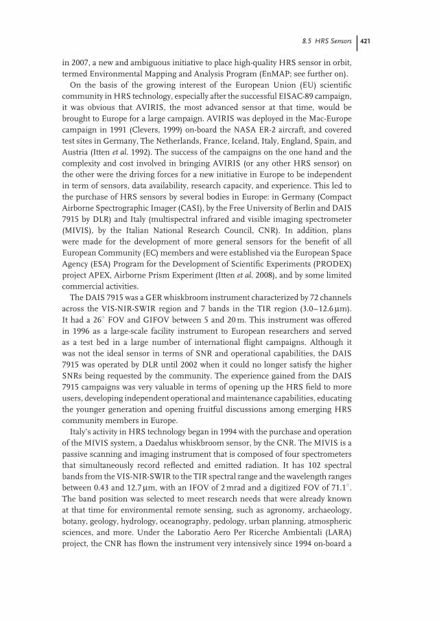
in 2007, a new and ambiguous initiative to place high-quality HRS sensor in orbit,termed Environmental Mapping and Analysis Program (EnMAP; see further on).
On the basis of the growing interest of the European Union (EU) scientificcommunity in HRS technology, especially after the successful EISAC-89 campaign,it was obvious that AVIRIS, the most advanced sensor at that time, would bebrought to Europe for a large campaign. AVIRIS was deployed in the Mac-Europecampaign in 1991 (Clevers, 1999) on-board the NASA ER-2 aircraft, and coveredtest sites in Germany, The Netherlands, France, Iceland, Italy, England, Spain, andAustria (Itten et al. 1992). The success of the campaigns on the one hand and thecomplexity and cost involved in bringing AVIRIS (or any other HRS sensor) onthe other were the driving forces for a new initiative in Europe to be independentin term of sensors, data availability, research capacity, and experience. This led tothe purchase of HRS sensors by several bodies in Europe: in Germany (CompactAirborne Spectrographic Imager (CASI), by the Free University of Berlin and DAIS7915 by DLR) and Italy (multispectral infrared and visible imaging spectrometer(MIVIS), by the Italian National Research Council, CNR). In addition, planswere made for the development of more general sensors for the benefit of allEuropean Community (EC) members and were established via the European SpaceAgency (ESA) Program for the Development of Scientific Experiments (PRODEX)project APEX, Airborne Prism Experiment (Itten et al. 2008), and by some limitedcommercial activities.
The DAIS 7915 was a GER whiskbroom instrument characterized by 72 channelsacross the VIS-NIR-SWIR region and 7 bands in the TIR region (3.0–12.6 μm).It had a 26◦ FOV and GIFOV between 5 and 20 m. This instrument was offeredin 1996 as a large-scale facility instrument to European researchers and servedas a test bed in a large number of international flight campaigns. Although itwas not the ideal sensor in terms of SNR and operational capabilities, the DAIS7915 was operated by DLR until 2002 when it could no longer satisfy the higherSNRs being requested by the community. The experience gained from the DAIS7915 campaigns was very valuable in terms of opening up the HRS field to moreusers, developing independent operational and maintenance capabilities, educatingthe younger generation and opening fruitful discussions among emerging HRScommunity members in Europe.
Italy’s activity in HRS technology began in 1994 with the purchase and operationof the MIVIS system, a Daedalus whiskbroom sensor, by the CNR. The MIVIS is apassive scanning and imaging instrument that is composed of four spectrometersthat simultaneously record reflected and emitted radiation. It has 102 spectralbands from the VIS-NIR-SWIR to the TIR spectral range and the wavelength rangesbetween 0.43 and 12.7 μm, with an IFOV of 2 mrad and a digitized FOV of 71.1◦.The band position was selected to meet research needs that were already knownat that time for environmental remote sensing, such as agronomy, archaeology,botany, geology, hydrology, oceanography, pedology, urban planning, atmosphericsciences, and more. Under the Laboratio Aero Per Ricerche Ambientali (LARA)project, the CNR has flown the instrument very intensively since 1994 on-board a
422 8 Hyperspectral Remote Sensing
CASA 212 aircraft, acquiring data mostly over Italy and also in cooperation withother nations, such as Germany, France, and the United States (Bianci et al. 1996).
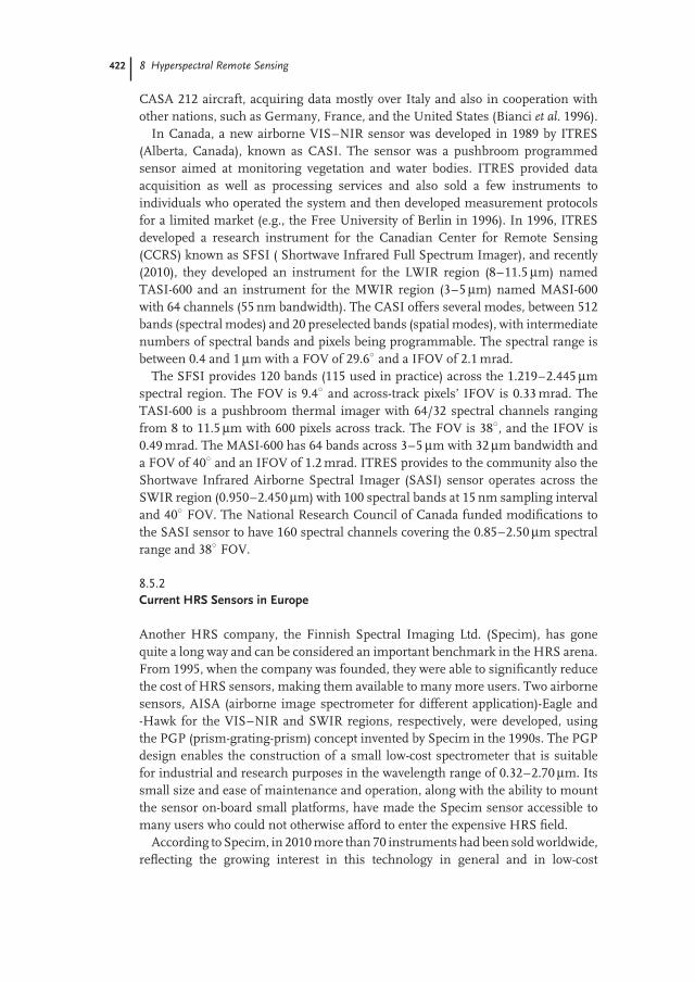
In Canada, a new airborne VIS–NIR sensor was developed in 1989 by ITRES(Alberta, Canada), known as CASI. The sensor was a pushbroom programmedsensor aimed at monitoring vegetation and water bodies. ITRES provided dataacquisition as well as processing services and also sold a few instruments toindividuals who operated the system and then developed measurement protocolsfor a limited market (e.g., the Free University of Berlin in 1996). In 1996, ITRESdeveloped a research instrument for the Canadian Center for Remote Sensing(CCRS) known as SFSI ( Shortwave Infrared Full Spectrum Imager), and recently(2010), they developed an instrument for the LWIR region (8–11.5 μm) namedTASI-600 and an instrument for the MWIR region (3–5 μm) named MASI-600with 64 channels (55 nm bandwidth). The CASI offers several modes, between 512bands (spectral modes) and 20 preselected bands (spatial modes), with intermediatenumbers of spectral bands and pixels being programmable. The spectral range isbetween 0.4 and 1 μm with a FOV of 29.6◦ and a IFOV of 2.1 mrad.
The SFSI provides 120 bands (115 used in practice) across the 1.219–2.445 μmspectral region. The FOV is 9.4◦ and across-track pixels’ IFOV is 0.33 mrad. TheTASI-600 is a pushbroom thermal imager with 64/32 spectral channels rangingfrom 8 to 11.5 μm with 600 pixels across track. The FOV is 38◦, and the IFOV is0.49 mrad. The MASI-600 has 64 bands across 3–5 μm with 32 μm bandwidth anda FOV of 40◦ and an IFOV of 1.2 mrad. ITRES provides to the community also theShortwave Infrared Airborne Spectral Imager (SASI) sensor operates across theSWIR region (0.950–2.450 μm) with 100 spectral bands at 15 nm sampling intervaland 40◦ FOV. The National Research Council of Canada funded modifications tothe SASI sensor to have 160 spectral channels covering the 0.85–2.50 μm spectralrange and 38◦ FOV.
8.5.2Current HRS Sensors in Europe
Another HRS company, the Finnish Spectral Imaging Ltd. (Specim), has gonequite a long way and can be considered an important benchmark in the HRS arena.From 1995, when the company was founded, they were able to significantly reducethe cost of HRS sensors, making them available to many more users. Two airbornesensors, AISA (airborne image spectrometer for different application)-Eagle and-Hawk for the VIS–NIR and SWIR regions, respectively, were developed, usingthe PGP (prism-grating-prism) concept invented by Specim in the 1990s. The PGPdesign enables the construction of a small low-cost spectrometer that is suitablefor industrial and research purposes in the wavelength range of 0.32–2.70 μm. Itssmall size and ease of maintenance and operation, along with the ability to mountthe sensor on-board small platforms, have made the Specim sensor accessible tomany users who could not otherwise afford to enter the expensive HRS field.
According to Specim, in 2010 more than 70 instruments had been sold worldwide,reflecting the growing interest in this technology in general and in low-cost
8.5 HRS Sensors 423
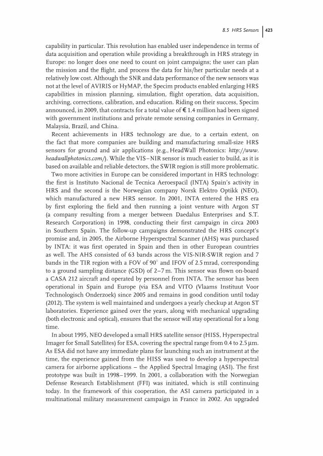
capability in particular. This revolution has enabled user independence in terms ofdata acquisition and operation while providing a breakthrough in HRS strategy inEurope: no longer does one need to count on joint campaigns; the user can planthe mission and the flight, and process the data for his/her particular needs at arelatively low cost. Although the SNR and data performance of the new sensors wasnot at the level of AVIRIS or HyMAP, the Specim products enabled enlarging HRScapabilities in mission planning, simulation, flight operation, data acquisition,archiving, corrections, calibration, and education. Riding on their success, Specimannounced, in 2009, that contracts for a total value of ¤ 1.4 million had been signedwith government institutions and private remote sensing companies in Germany,Malaysia, Brazil, and China.
Recent achievements in HRS technology are due, to a certain extent, onthe fact that more companies are building and manufacturing small-size HRSsensors for ground and air applications (e.g., HeadWall Photonics: http://www.headwallphotonics.com/). While the VIS–NIR sensor is much easier to build, as it isbased on available and reliable detectors, the SWIR region is still more problematic.
Two more activities in Europe can be considered important in HRS technology:the first is Instituto Nacional de Tecnica Aeroespacil (INTA) Spain’s activity inHRS and the second is the Norwegian company Norsk Elektro Optikk (NEO),which manufactured a new HRS sensor. In 2001, INTA entered the HRS eraby first exploring the field and then running a joint venture with Argon ST(a company resulting from a merger between Daedalus Enterprises and S.T.Research Corporation) in 1998, conducting their first campaign in circa 2003in Southern Spain. The follow-up campaigns demonstrated the HRS concept’spromise and, in 2005, the Airborne Hyperspectral Scanner (AHS) was purchasedby INTA: it was first operated in Spain and then in other European countriesas well. The AHS consisted of 63 bands across the VIS-NIR-SWIR region and 7bands in the TIR region with a FOV of 90◦ and IFOV of 2.5 mrad, correspondingto a ground sampling distance (GSD) of 2–7 m. This sensor was flown on-boarda CASA 212 aircraft and operated by personnel from INTA. The sensor has beenoperational in Spain and Europe (via ESA and VITO (Vlaams Instituut VoorTechnologisch Onderzoek) since 2005 and remains in good condition until today(2012). The system is well maintained and undergoes a yearly checkup at Argon STlaboratories. Experience gained over the years, along with mechanical upgrading(both electronic and optical), ensures that the sensor will stay operational for a longtime.
In about 1995, NEO developed a small HRS satellite sensor (HISS, HyperspectralImager for Small Satellites) for ESA, covering the spectral range from 0.4 to 2.5 μm.As ESA did not have any immediate plans for launching such an instrument at thetime, the experience gained from the HISS was used to develop a hyperspectralcamera for airborne applications – the Applied Spectral Imaging (ASI). The firstprototype was built in 1998–1999. In 2001, a collaboration with the NorwegianDefense Research Establishment (FFI) was initiated, which is still continuingtoday. In the framework of this cooperation, the ASI camera participated in amultinational military measurement campaign in France in 2002. An upgraded
424 8 Hyperspectral Remote Sensing
version of the instrument was flown in 2003 and 2004 in different multinationalmilitary field trials. In 2004, airborne HRS data were also acquired for severallocal civilian research institutions. The cooperation with these institutions wascontinued in 2005 when a further upgraded version of the instrument was flownsuccessfully, including a HRS camera module covering the part of SWIR region(0.9–1.7 μm), in addition to the VIS and NIR regions (0.4–1.0 μm).
All these research activities led to the development of a line of hyperspectralcameras (HySpex) that are well suited for a wide variety of applications in both thecivilian and military domains. Main characteristics of the sensor are coverage ofthe entire range (0.4–2.5 μm) with more than 400 bands with 3.7 and 6.25 nm bandwidth two different sensors (the VNIR 640 and SWIR 320). The sensor underwentseveral experiments in Europe with proven success but has not yet aggressivelyentered the commercial remote sensing arena.
Beside the AVIRIS sensor, today the HyMAP sensor has become available: this isa commercially designed and operated system that was based on the Probe-1 sensor(operated in circa 1998 by Applied Signal and Image Technology (ASIT), USA).Several campaigns in the United States demonstrated the promising commercialcapability of HRS technology (Kruse et al. 2000). Integrated Spectronics, Australia,designed and operated the HyMAP sensor for rapid and efficient wide-area imagingfor mineral mapping and environmental monitoring. The sensor can be definedas a high SNR instrument with high spectral resolution, ease of use, a modulardesign concept, calibrated spectroradiometry, proven in-field operation, and heavyload capacity. It is a whiskbroom sensor with 100–200 bands (usually 126) acrossthe 0.45–2.45 μm spectral region with bandwidths ranging from 10 to 20 nm.
The SNR is in the range of 500 : 1 with 2–10 m spatial resolution. It is charac-terized by a 60◦ –70◦ swath width and furnished with an on-board radiometric andspectral calibration assembly. In 1999, a group shoot using the HyMAP sensor wasconducted in the United States. A report by Kruse et al. (2000) declared the sensor tobe the best available at the time. Since then, the HyMAP sensor has been operatedworldwide, providing high-quality HRS data to its end users and opening up anew era in HRS data quality. It has been operated in Europe, Australia, the UnitedStates, Asia and Africa in specific campaigns and through Hy Vista activity, whichprovides end-to-end solutions for the potential customer. HyMAP can thus also beconsidered a benchmark in HRS technology, which was reached in circa 1999 byProbe-1 and then afterwards by HyMAP sensors. The problem with HyMAP is thatthe sensor is limited and is operated only by HyVista, and hence, its use is stronglydependent on their schedule and availability. Moreover, the cost of the data is stillprohibitive for the daily use capability that is desired from HRS technology. It canbe concluded that there is still a significant gap between high SNR and low cost/easyoperation in sensors: ideally, this gap might be bridged by fusing the AISA andHyMAP characteristics that are based on two different technologies: pushbroomand whiskbroom, respectively. As more and more companies undertake movingHRS technology forward, we believe that in the near future such a fusion will bepossible and we will see more low-cost, high-quality data and more applicationsemerging from this capability.
8.5 HRS Sensors 425
In 2011, the APEX has become available to the European research communityafter a long prototyping and development (Itten et al. 2008). It has been built inESA’s Prodex program by Swiss–Belgium collaborative efforts and is operatedby VITO, Belgium. This system may be considered a new breakthrough in HRStechnology, as it is the first airborne pushbroom system offering a completecoverage of the spectral range between 0.4 and 2.5 μm in one integrated system.APEX provides the same spatial resolution of 1–5 m at 1000 across-track pixels forboth the VIS–NIR and SWIR spectral range. The prism design optics allows forvery high spectral resolution in the visible part down to 1 nm, whereas the SWIRis resolved with 7 nm. Its data is currently evaluated for various IS applicationsand the system is to be used for cross-calibration purposes for ESA satellites andalike.
The above provides only the milestone stages in HRS technology over theyears. Several of the sensors and activities may not have been mentioned.The reader is therefore directed to a comprehensive description of all HRSsensors until 2008 made by Prof. Gomez from George Mason Universityin the United States and to a summary of all remote sensing organizationsworldwide and all institutes, private sectors, and abbreviations commonlyused with this technology at http://www.tau.ac.il/∼rslweb/pdf/HSR.pdf. Ahistorical list of HRS sensors compiled by Michael Schaepman is available athttp://www.geo.unizh.ch/∼schaep/research/apex/is_list.html.
8.5.3Satellite HRS Sensors
Among the airborne HRS benchmarks mentioned earlier, orbital HRS activityhas contributed greatly to the blossoming HRS activity. The first initiative toplace an HRS sensor in orbit took place in the early 1990s when a group ofscientists chaired by Goetz started work on the NASA HRS mission HIRIS (HighResolution Imaging Spectrometer). This was part of NASA’s High-ResolutionImaging Spectrometer Earth Observation System program. The idea was to placean AVIRIS-like sensor in orbit with a full range between 0.4 and 2.5 μm anda spatial resolution of 30 m. A report that provides the capacity of this sensor,including its technical and application characteristics, was issued in several copies(Goetz, 1987). This report was the first document that showed the intention togo into space with HRS. The HIRIS mission was terminated, apparently becauseof the Challenger space shuttle disaster, which significantly changed the spaceprograms at NASA.
The scientists, however, agreed that using HRS in orbit is an important taskthat needs to be addressed (Nieke et al. 1997). A report by Hlao and Wong (2000)submitted to the US Air Force in 2000 assessed the technology as premature andstill lagging behind other remote sensing technologies such as air photography.The next benchmark in orbital HRS was Hyperion, part of the NASA NewMillennium Program (NMP). The Hyperion instrument was built by TRW Inc.
426 8 Hyperspectral Remote Sensing
(Thompson Ramo Woddbridge) using focal planes and associated electronicsremaining from the Lewis spacecraft, a product of the NASA Small SatelliteTechnology Initiative (SSTI) mission that fell in 1997. The integration of Hyperiontook less than 12 months from Lewis’s spare parts and was sent into orbit on-boardthe EO-1 spacecraft. The mission, planned for 3 years, is still operational today(2012) with a healthy sensor and data, although the SNR is poor. The instrumentcovers the VIS-NIR-SWIR region from 0.422 to 2.395 μm with two detectors and244 bands of 10 nm bandwidth. The ground coverage FOV provided a 7.5 km swathand 30 m GSD. The first data sets cost around US$2500 and had a lower SNRthan originally planned. Nonetheless, over the years, and despite its low quality,the instrument has brought new capability to sensing the globe by temporalHRS coverage, justifying the effort to place a better HRS sensor in space. Asof the summer of 2009, Hyperion data are free of charge, which has openedup a new era for potential users. In circa 2001, the CHRIS (Compact HighResolution Imaging Spectrometer) sensor was launched into orbit on-board thePROBA (Project on Board Autonomy) bus. It was developed by the Sira ElectroOptic group and supported by the ESA. The CHRIS sensor is a high spatialresolution hyperspectral spectrometer (18 m at nadir) with a FOV resulting in14 km swath.
One of its most important characteristics is the possibility of observing everyground pixel at the same time, in five different viewing geometry sets (nadir, ±55◦
and ±36◦). It is sensitive to the VIS–NIR region (0.41–1.059 μm), and the numberof bands is programmable, with up to 63 spectral bands. Although limited in itsspectral region, the instrument provides a first view of the bidirectional reflectancedistribution function (BRDF) effects for vegetation and water applications, and itis robust, as it is still operating today. The ‘‘early’’ spaceborne planning missionsin both the United States and Europe comprised, among others, the followingprojects: IRIS (Interface Region Imagery Spectrograph), HIRIS (NASA), GEROS(German Earth Resources Observer System, USA), HERO (Hyperspectral Environ-mental and Resource Observer, CSA), PRISM (Process Research by an ImagingSpace Mission), SPECTRA (Surface Processes and Ecosystem Changes ThroughResponse Analysis, all ESA), SIMSA (Spectral Imaging Mission for Science) andSAND (Spectral Analysis of Dryland). Although most of these initiatives were notfurther funded and are not active today, they demonstrated government agen-cies’ interest in investing in this technology, albeit with a fearful and cautiousattitude. Other orbital sensors, such as MODIS (Moderate Resolution ImagingSpectrometer), MERIS (Medium Resolution Imaging Spectrometer), and ASTER(Advanced Spaceborne Thermal Emission and Reflection), can also be consid-ered part of the HRS activities in space, but in terms of both spatial (MODISand MERIS) and spectral (ASTER) resolution, these sensors and projects stilllag behind the ideal HRS sensor that we would like to see in orbit with highspectral (more than 100 narrow bands) and spatial (less than 30 m) resolutions.It is important to mention, however, that a new initiative to study the moon andMars using HRS technology took place by a collaboration between NASA andISA (India), within which the M3 mission to the moon has recently provided
8.5 HRS Sensors 427
remarkable results by mapping a thin layer of water on the moon’s surface (Pieterset al. 2009b,a). In addition, missions to Mars, such as CRISM (Compact Recon-naissance Imaging Spectrometer for Mars) show that it is now understood thatHRS technology can provide remarkable information about materials and objectsremotely.
EnMAP is a German hyperspectral satellite mission providing high-qualityhyperspectral image data on a timely and frequent basis. Its main objective isto investigate a wide range of ecosystem parameters encompassing agriculture,forestry, soil and geological environments, coastal zones, and inland waters. Thiswill significantly increase our understanding of coupled biospheric and exosphericprocesses, thereby enabling the management and guaranteed sustainability of ourvital resources. Launch of the EnMAP satellite is envisaged for 2015 (updatedin 2012). The basic working principle is that of a pushbroom sensor, whichcovers a swath (across-track) width of 30 km, with a GSD of 30 × 30 m. Thesecond dimension is given by the along-track movement and corresponds to about4.4 ms exposure time. This leads to a detector frame rate of 230 Hz, which is aperformance-driving parameter for the detectors, as well as for the instrumentcontrol unit and the mass memory. HyspIRI is a new NASA initiative to place aHRS sensor in orbit and is aimed at complementing EnMAP, as its data acquisitioncovers the globe periodically.
It is important to mention that other national agencies are aiming to placeHRS sensor in orbit as well. A good example is PRISMA of the Italy’s spaceagency. PRISMA is a pushbroom sensor with swath of 30–60 km, GSD of 20–30 m(2.5–5 m peroxyacetylnitrate (PAN)) with a spectral range of 0.4–2.5 μm. Thesatellite launch was foreseen by the end of 2013, but it seems that some delay isencountered and the new lunch date is unknown.
To keep everyone up to date and oriented on the efforts being made inHRS pace activities, a volunteer group was founded in November 2007 byDr Held and Dr Staenz named ISIS (International Satellite Imaging Spec-trometry) (Staenz, 2009). The ISIS group provides a forum for technical andprogramming discussions and consultation among national space agencies, re-search institutions, and other spaceborne HRS data providers. The main goalsof the group are to share information on current and future hyperspectralspaceborne missions and to seek opportunities for new international partner-ships to the benefit of the global user community. The initial ‘‘ISIS WorkingGroup’’ was established following the realization that there were a large num-ber of countries planning HRS (‘‘hyperspectral’’) satellite missions with littlemutual understanding or coordination. Meetings of the working group havebeen held in Hawaii (IGARSS 2007), Boston (IGARSS 2008), Tel Aviv (EARSeL2009), Hawaii (IGARSS 2010), Vancouver (IGARSS 2011) and Munich (IGARSS2012). The technical presentations by the ISIS group have garnered interestfrom space agencies and governmental and industrial sectors in this promisingtechnology. An excellent review on current and planned civilian space hyper-spectral sensor for Earth observation (EO) is given by Buckingham and Staenz(2008).
428 8 Hyperspectral Remote Sensing
8.6Potential and Applications
Merging of spectral and spatial information, as is done within HRS technology,provides an innovative way of studying many spatial phenomena at various res-olutions. If the data are of high quality, they allow near-laboratory level spectralsensing of targets from afar. Thus, the information and knowledge gathered in thelaboratory domain can be used to process the HRS data on a pixel-by-pixel basis.The ‘‘spheres’’ that can feasibly be assessed by HRS technology are atmosphere,pedosphere, lithosphere, biosphere, hydrosphere, and cryosphere. Different meth-ods of analyzing the spectral information in the HRS data are known, the basicone consisting of comparing the pixel spectrum with a set of spectra taken froma well-known spectral library. This allows the user to identify specific substances,such as minerals, chlorophyll, dissolved organics, atmospheric constituents, andspecific environmental contaminants, before moving ahead with other more so-phisticated approaches (Section 8.8.4). The emergence of hyperspectral imagingmoved general remote sensing applications from the area of basic landscape clas-sification into the realm of full spectral quantification and analysis. The same typeof spectroscopy applications that have been utilized for decades by chemists andastronomers are now accessible through both nadir and oblique viewing applica-tions. The spectral information enables the detection of indirect processes, suchas contaminant release, based on changes in spectral reflectance of the vegetationor leaves. The potential thus lies in the spectral recognition of targets using theirspectral signature as a footprint and on the spectral analysis of specific absorptionfeatures that enable a quantitative assessment of the matter in question. Althoughmany applications remain to be developed, within the past decade, significantadvances have been made in the development of applications using hyperspectraldata, mainly because of the extensive availability of today’s airborne sensors. While,a decade ago, only a few sensors were available and used in the occasional cam-paign, today, many small and user-friendly HRS sensors that can operate on anylight aircraft are available.
Hydrology, disaster management, urban mapping, atmospheric study, geology,forestry, snow and ice, soil, environment, ecology, agriculture, fisheries, and oceansand national security are only a few of the applications for HRS technology today.In 2001, van der Meer and Jong (2001) published a book with several innovativeapplications for that time. Since then, new applications have emerged and thepotential of HRS has been discussed and analyzed by many authors at conferences,in proceedings papers and full-length publications. In a recent paper, Staenz (2009)provides his present and future notes on HRS, which very accurately summarize thetechnology up to today. In the following, we paraphrase and sharpen Staenz’s points.It is clear from the numerous studies that have been carried out that HRS technologyhas significantly advanced the use of remote sensing in different applications (e.g.,AVIRIS 2007). In particular, the ability to extract quantitative information has madeHRS a unique remote sensing tool. For example, this technology has been used bythe mining industry for exploration of natural resources, such as the identification
8.6 Potential and Applications 429
and mapping of the abundance of specific minerals. HRS is also recognized as a toolto successfully carry out ecosystem monitoring, especially the mapping of changesbecause of human activity and climate variability. This technology also plays animportant role in the monitoring of coastal and inland waters. Other capabilitiesinclude the forecasting of natural hazards, such as mapping the variability of soilproperties that can be linked to landslide events, and monitoring environmentaldisturbances, such as resource exploitation, forest fires, insect damage, and slopeinstability in combination with heavy rainfall. As already mentioned, HRS can beused to assess quantitative information about the atmosphere such as water vaporcontent; aerosol load; and methane, carbon dioxide, and oxygen content. HRS canalso be used to map snow parameters, which are important in characterizing a snowpack and its effect on water runoff. Moreover, the technology has shown potentialfor use in national security, for example, in surveillance and target identification,verification of treaty compliance (e.g., Kyoto Accord on Greenhouse Gas Emission),and disaster preparedness and monitoring (Staenz, 2009). Some recent examplesshow both the quantitative and exclusive power of HRS technology in detection ofsoil contamination (Kemper and Sommer, 2003), soil salinity (Ben-Dor et al. 2002),species of vegetation (Ustin et al. 2008), atmospheric electromagnetic emissionsof methane (Noomem, Meer, and Skidmore, 2005), detection of ammonium(Gersman et al. 2008), asphalt condition (Herold et al. 2008), water quality (Dekkeret al. 2001), and urban mapping (Ben-Dor, 2001). Many other applications can befound in the literature and still others are in the R&D phase in the emergingHRS community. Nonetheless, although promising, one should remember thatHRS technology still suffers from some difficulties and limitations. For example,the large amount of data produced by the HRS sensors hinders this technology’susefulness for geometry analysis or visual cognition (e.g., building structures androads) and one has to weight the added value promised by the technology forone’s applications. There are other remote sensing tools and the user shouldconsult with an expert before using HRS technology. Since the emergence ofHRS, many technical difficulties have been overcome in areas such as sensordevelopment, data handling, aviation and positioning, and data processing andmining. However, there are several main issues that require solutions to movethis technology toward more frequent operational use today. These include a lackof reliable data sources with a high SNR are required to retrieve the desiredinformation and temporal coverage of the region of interest; although analyticaltools are now readily available, there is a lack of robust automated procedures toprocess data quickly with a minimum of user intervention; the lack of operationalproducts is obviously due to the fact that most efforts to date have been devotedto the scientific development of HRS; interactions with other HRS communitieshave not yet developed – there are many applications, methods, and know-howin the laboratory-based HRS disciplines but no valid connection between thecommunities; systems that can archive and handle large amounts of data andopenly share the information with the public are still lacking; only a thin layer ofthe surface can be sensed; there is no standardization for data quality or qualityindicators (QI); not much valid experience exists in merging HRS data with that
430 8 Hyperspectral Remote Sensing
of other sensors (e.g., LIDAR, SAR (Synthetic Aperture RADAR)); many sensorshave emerged in the market but their exact operational mechanism is unknown,biasing an accurate assessment; thermal HRS sensors are just starting to emerge,whereas point thermal spectrometers are existing (Christensen et al. 2000); obliqueview and ground-based HRS measurements have not yet been frequently used; thecost of deriving the information product is too high, since the analysis of HRSdata is currently too labor intensive (not yet automated); it is not yet recognizedby potential users as a routine vehicle as, for example, is air photography; not toomany experts in this technology are available. Several authors have summarizedthis technology’s potential to learn from history, such as Itten (2007); Schaepmanet al. (2009) and Staenz (2009).
It is anticipated that HRS technology will catch up when new high-quality sensorsare placed in orbit and the data become available to all (preferably in reflectancevalues), when the air photography industry uses the HRS data commercially, andwhen new sensors that are inexpensive and easy to use are developed along withinexpensive aviation (such as unmanned aerial vehicle, UAV).
8.7Planning of an HRS Mission
In this section, we describe major issues for the planning of a mission for anairborne campaign: we do not cover the possible activities involved for a spacebornemission. Planning a mission is a task that requires significant preparation andknowledge of the advantages and disadvantages of the technology. The idea behindusing HRS is to get an advanced thematic map as the final product which no othertechnology can provide. In the planner’s mind, the major step toward achievingthe main prerequisite of a thematic map is to generate a reflectance or emissionimage from the raw data.
First, a scientific (or applicable) question has to be asked, such as Where cansaline soil spots be found over a large area? For such a mission, the user has to deter-mine whether there exists spectral information on the topic which is being coveredby the current HRS sensor. This investigation might consist of self-examinationor a literature search of both the area in question and the advantageous of usingHRS (many times, HRS is an overkill technology for answering simple thematicquestions). Once this investigation is carried out, the question is What are theexact spectral regions that are important for the phenomenon in question andwhat pixel size is needed? In addition, the question of what SNR values will enablesuch detection should be raised. Having this information in hand, the next step isto search for the instrument. Sometimes, a particular instrument is available, andthere is no other choice. In this case, the first spectral investigation stage shouldfocus on the available HRS sensor and its spectral performances (configuration,resolution, SNR, etc.) infrastructure. It is recommended that the spectralinformation on the thematic question be checked at the sensor-configuration
8.7 Planning of an HRS Mission 431
stage. In some sensors, especially pushbroom ones, it is possible to program thespectral configuration using a new arrangement of the CCD assembly.
In this respect, it is important that the flight altitude be taken into consideration(for both pixel size and integration time) along with aircraft speed. Most sensorshave tables listing these components and the user can use them to plan the missionframe. As within this issue, the user can configure the bands with different FWHMand positions; it should be remembered that combined with spatial resolution,this might affect the SNR. When selecting the sensor, it is important to obtain(if this is the first use) a sample cube to learn about the sensor’s performance. Itis also good to consult with other people who have used this equipment. Gettinginformation on when and where the last radiometric calibration was performedas well as obtaining information about the sensor stability and uncertainties isvery important. It is better if the calibration file of the sensor is provided but ifnot, the HRS owner should be asked for the last calibration date and its temporalperformances.
Quality assurance (QA) of the sensor’s radiance must be performed in order toassure a smooth step to the next stage, namely, atmospheric correction. Methodsand tools to inspect these parameters were developed under EUFAR JRA2 initiativeand recently also by Brook and Ben-Dor (2011).
The area in question is generally covered by 30% overlap between the lines. Thishas to be carefully planned in advance taking into consideration the swath of thesensor and other aircraft information (e.g., stability, time in the air, speed andaltitude preferences, navigation systems). A preference for flying toward or againstthe direction of the Sun’s azimuth needs to be decided on, and it is recommendedthat the Google Earth interface be used to allocate the flight lines and to provide atable for each line with starting and ending points for all flight lines. One also needsto check if the GPS is available and configure the system to be able to ultimatelyallocate this information in a readable and synchronized form.
A list of go/no go items should be established. For instance, a forecast for theweather should be on hand 24 h in advance, with updates every 3 h. If possible, arepresentative should be sent to the area in question to report on cloud coverageclose to acquisition time. In our experience, one should be aware of the fact that a1/2 cover over the area in question will turn into almost 100% coverage of the flightlines that appeared to be free of clouds. Moreover, problems that may emerge atthe airport need to be taken into consideration, such as the GPS is not functioningor the altitude obtained from air control is different from that which was planned.The go/no go checklist should be used for these issues as needed. Each go/no golist is individual, and one should be established for every mission.
The aircrew members (operators, navigator, and pilot) must be briefed beforeand debriefed after the mission. A logbook document should be prepared for theaircrew members (pilot and operator) with every flight line reported by them. It isimportant to plan a dark current acquisition before and after each line acquisition.Acquisition of a vicarious calibration site (in the area of interest or on the way to thisarea) in question should also be planned for, that is well prepared and documentedin advance. If possible, radio contact with the aircrew should be obtained at a
432 8 Hyperspectral Remote Sensing
working frequency before, during, and after the overpass. A ground team shouldbe prepared and sent to the area in question for the following issues: (i) calibratingthe sensor’s radiance and examining its performance (Brook and Ben-Dor, 2011),(ii) validating the atmospheric correction procedure, and (iii) collecting spectralinformation that will be useful further on for thematic mapping (e.g., chlorophyllconcentration in the leaves). The ground team should be prepared according toa standard protocol, and it should be assured that they are furnished with thenecessary equipment (such as video and still cameras, field spectrometer, maps,Sun photometer, and GPS). After data acquisition both from air and ground, thedata should be immediately backed up and quality control checks run to determinedata reliability. Afterward, the pilot logbook, ground documentation, and any othermaterial that evolved during the mission should be collected.
In general and to sum up the above, a mission has to be lead by a senior personwho is responsible to coalesce the end user needs, the ground team work, theairborne crew activity, and the processing stages performed by experts. He/she isresponsible to interview the end user and understand the question at hand and isresponsible to allocate a sensor for the mission and meet with the sensor ownerand operator ahead of the mission and arrange a field campaign by a ground team.Other responsibilities such as arranging logistics and briefing of all teams as wellas backing up the information just after the mission end, that is, at the airportare also part of their duties and are very important. A checklist and documents onevery stage are available in many bodies (e.g., DLR, TAU, the Tel Aviv University),but in general, it can be developed by any group by gathering information frommain HSR leading bodies (DLR, NASA, INTA).
8.8Spectrally Based Information
A remotely sensed object interacts with electromagnetic radiation where photonsare absorbed or emitted via several processes. On the Earth’s surface (solid andliquid) and in its atmosphere (gasses and aerosol particles), the interaction across theUV-VIS-NIR-SWIR-TIR regions is sensed by HRS means to give additional spectralinformation relative to the common multiband sensors. The spectral response of theelectromagnetic interaction with matter can be displayed as radiance, reflectance,transmittance, or emittance, depending on the measurement technique and theillumination source used. Where interactions occur, a spectrum shape can be usedas a footprint to assess and identify the matter in question. Variations in the positionof local minima (or maxima, termed ‘‘peaks’’) and baseline slope and shape arethe main indicators used to derive quantitative information on the sensed material.The substance (chemical or physical) that significantly affects the shape and natureof the target’s spectrum is termed ‘‘chromophore.’’ A chromophore that is activein energy absorptance (e.g., chlorophyll molecule in vegetation) or emission (e.g.,fluorescence) at a discrete wavelength is termed a ‘‘chemical chromophore.’’ Achromophore that governs the spectrum’s shape (such as the slope and albedo
8.8 Spectrally Based Information 433
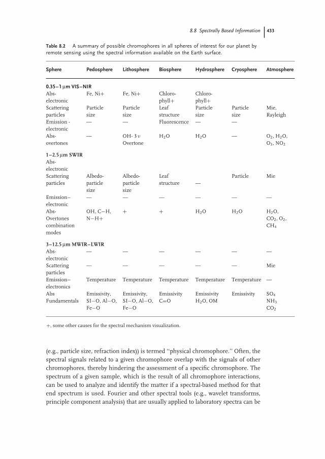
Table 8.2 A summary of possible chromophores in all spheres of interest for our planet byremote sensing using the spectral information available on the Earth surface.
Sphere Pedosphere Lithosphere Biosphere Hydrosphere Cryosphere Atmosphere
0.35–1 μm VIS–NIRAbs- Fe, Ni+ Fe, Ni+ Chloro- Chloro-electronic phyll+ phyll+Scattering Particle Particle Leaf Particle Particle Mie,particles size size structure size size RayleighEmission - — — Fluorescence — —electronicAbs- — OH- 3 ν H2O H2O — O2, H2O,overtones Overtone O3, NO2
1–2.5 μm SWIRAbs-electronicScattering Albedo- Albedo- Leaf Particle Mieparticles particle particle structure —
size sizeEmission– — — — — — —electronicAbs- OH, C−H, + + H2O H2O H2O,Overtones N−H+ CO2, O2,combination CH4
modes
3–12.5 μm MWIR–LWIRAbs- — — — — — —electronicScattering — — — — — MieparticlesEmission– Temperature Temperature Temperature Temperature Temperature —electronicsAbs Emissivity, Emissivity, Emissivity Emissivity Emissivity SO4
Fundamentals SI−O, Al−O, SI−O, Al−O, C=O H2O, OM NH3
Fe−O Fe−O CO2
+, some other causes for the spectral mechanism visualization.
(e.g., particle size, refraction index)) is termed ‘‘physical chromophore.’’ Often, thespectral signals related to a given chromophore overlap with the signals of otherchromophores, thereby hindering the assessment of a specific chromophore. Thespectrum of a given sample, which is the result of all chromophore interactions,can be used to analyze and identify the matter if a spectral-based method for thatend spectrum is used. Fourier and other spectral tools (e.g., wavelet transforms,principle component analysis) that are usually applied to laboratory spectra can be
434 8 Hyperspectral Remote Sensing
excellent tools for application to HRS data provided the data are of good quality. Acomprehensive review of chemical and physical chromophores in soils and rocks,as an example, can be found in Irons, Weismiller, and Petersen (1989); Ben-Dor,Irons, and Epema (1999); Clark (1999); Malley, Martin, and Ben-Dor (2004);McBratney and Rossel (2006). A compilation table that provides the chromophoresof known Earth targets in all spheres is given in Table 8.2. The table, which coversall spectral regions (VIS, NIR, SWIR, MWIR, and LWIR), may be of interest forHRS technology from field, air, and space levels.
The chemical chromophores in the VIS-NIR-SWIR regions refer to two basicchemical mechanisms: (i) overtones and combination modes in the NIR–SWIRregion that emerge from the fundamental vibrations in the TIR regions and(ii) electron processes in the VIS region that are in most cases crystal-field andcharge-transfer effects. The physical chromophores in this region refer mostly toparticle size distribution and to refraction indices of the matter in question. Theelectronic processes are typically affected by the presence of transition metals,such as iron, and although smeared, they can be used as a diagnostic feature foriron minerals (around 0.80–0.90 μm crystal field and around 0.60–0.70 μm chargetransfer).
Accordingly, all features in the UV-VIS-NIR-SWIR-TIR spectral regions havea clearly identifiable physical basis. In solid–fluid Earth materials, three majorchemical chromophores can be roughly categorized as follows: (i) minerals (mostlyclay, iron oxide, primary minerals-feldspar, Si, insoluble salt, and hard-to-dissolvesubstances such as carbonates, and phosphates), (ii) organic matter (living anddecomposing), and (iii) water (solid, liquid, and gas phases). In gaseous Earthmaterials, the two main chemical chromophores are (i) gas molecules and (ii)aerosol particles of minerals, organic matter, and ice.
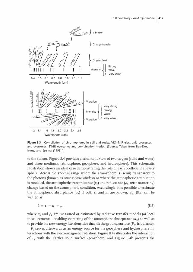
Figure 8.3 presents a summary of possible chromophores in soils and rocks(Ben-Dor, Irons, and Epema, 1999). Basically, the (passive) electromagnetic sourcesfor HRS are the radiation of Sun and Earth (terrestrial) (Sun: VIS-NIR-SWIR, Sunand Earth: TIR). Assuming that in a photon pack emitted from a given source(F; F0 for Sun, Fe for Earth), some photons may be absorbed (Fα), reflected (Fρ ),or transmitted (Fτ ) at a given wavelength and incident angle. The energy balance(in terms of flux densities) on a given target for every boundary (atmosphere,geosphere, and hydrosphere) can be written as follows:
F = Fτ + Fα + Fρ (8.1)
where F = F0 + Fe or any other incident light hitting the target (e.g., Fg, Fwf , andFws for ground, water floor, and water surface, respectively; Figure 8.4a,b). If weassume that we know the source energy (e.g., F0), dividing Eq. (8.1) by F0 gives
1 = τ + α + ρ (8.2)
where τ is the transmittance, α the absorptance, and ρ the reflectance coefficients,respectively. These coefficients describe the proportion of Fτ , Fα , and Fρ , respec-tively and range from 0 to 1. In an ideal cases, the Sun emits photons (F0) thatpass through the atmosphere and hit the ground (Fg) and then are reflected back
8.8 Spectrally Based Information 435
Wavelength (μm)
0.4 0.5 0.6 0.7 0.8 0.9 1.0 1.1
IntensityStrongWeakVery weak
Crystal field
Charge transfer
Vibration
Ti3+ Ti4
+
Fe2+ Fe3+
3u (OH-Me)
2u1 + n2 (H2O)F
e3+6 A
1g4 E
g(4 A
1 g)F
e2+
5 T2g
3 T1g
Fe
2+5 T 2g
3T 1g
Fe
2+ 5T
1 A 1gFe
2+5 T 2g
3 T 1g
Fe3+
5 T 2g3 T 1g
Fe3+
6 A 1g4 T 1g
Fe2+ E
g T
2g
Wavelength (μm)
1.2 1.4 1.6 1.8 2.0 2.2 2.4 2.6
Intensity StrongWeak
Very weak
Vibration
Vibration
Very strong
u1+
u2+
u3
(H2O
)
2u3
+u 2
(H
2O
)
u1+ 2u3
; 3u1+ u1(CO3
−)
u+ d (OH-F
e;υ 3
(CO 3
− )
u1+
2υ3 (
CO
3− )
n + 2d(OH-P)
n+ d(O
H-Al)
n+d
(OH
-Mg)
n+δ (
OH
-P)
n (H
2O
)
u 1+
3u 3 (C
O 3− )
2u1+ 2u3 (CO3
−)u 1
+ u 3 (H 2
O)
u 1+ u 3
(H2O)
n 1+ 2n
3 (H
2O)
n 1+ n 2
+ n 3 (C
O 3− )
2n+δ
(OH
-P)
2n (O
H-F
e)
2n-
(OH
-Al)
Figure 8.3 Compilation of chromophores in soil and rocks: VIS–NIR electronic processesand overtones, SWIR overtones and combination modes. (Source: Taken from Ben-Dor,Irons, and Epema (1999).)
to the sensor. Figure 8.4 provides a schematic view of two targets (solid and water)and three mediums (atmosphere, geosphere, and hydrosphere). This schematicillustration shows an ideal case demonstrating the role of each coefficient at everysphere. Across the spectral range where the atmosphere is (semi) transparent tothe photons (known as atmospheric window) or where the atmospheric attenuationis modeled, the atmospheric transmittance (τa) and reflectance (ρa, term scattering)change based on the atmospheric condition. Accordingly, it is possible to estimatethe atmospheric absorptance (αa) if both τa and ρa are known; Eq. (8.2) can bewritten as
1 = τa + αa + ρa (8.3)
where τa and ρa are measured or estimated by radiative transfer models (or localmeasurements), enabling extracting of the atmosphere absorptance (αa) as well asto provide the new energy flux densities that hit the ground surface (Fg, irradiance).
Fg serves afterwards as an energy source for the geosphere and hydrosphere in-teractions with the electromagnetic radiation. Figure 8.4a illustrates the interactionof Fg with the Earth’s solid surface (geosphere) and Figure 8.4b presents the
436 8 Hyperspectral Remote Sensing
Atm
osphereG
eosphereS
paceA
tmosphere
Hydro-G
eo-sphere sphere
τa
τa
αa
αa
Fe Fg
F0
F0
αgT, ε
Fg = Fws
T
τg
τwf
ρwf
Fe
+
ρg
ε = 1
αwf
τwbαwb
ρwb
ρws
ρw
Fwf
ρa
ρa
(a)
(b)
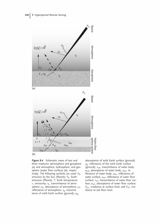
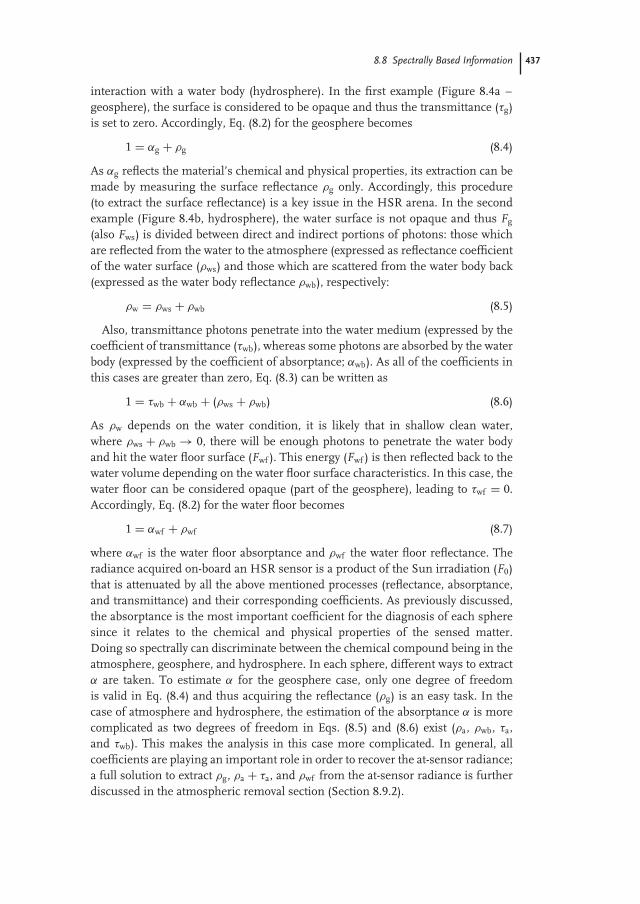
Space
Figure 8.4 Schematic views of two andthree mediums (atmosphere and geosphere(a) and atmosphere, hydrosphere, and geo-sphere (water floor surface) (b), respec-tively). The following symbols are used: F0,emission by the Sun (Planck); Fe, Earthemission (Planck); T, Earth temperature;ε, emissivity; τa, transmittance of atmo-sphere; αa, absorptance of atmosphere; ρa,reflectance of atmosphere; τg, transmit-tance of solid Earth surface (ground); αg,
absorptance of solid Earth surface (ground);ρg, reflectance of the solid Earth surface(ground); τwb, transmittance of water body;αwb, absorptance of water body; ρwb, re-flectance of water body; ρws, reflectance ofwater surface; ρwf , reflectance of water floorsurface; τwf , transmittance of water floor sur-face; αwf , absorptance of water floor surface;Fws, irradiance at surface level; and Fwf , irra-diance at sea floor level.
8.8 Spectrally Based Information 437
interaction with a water body (hydrosphere). In the first example (Figure 8.4a –geosphere), the surface is considered to be opaque and thus the transmittance (τg)is set to zero. Accordingly, Eq. (8.2) for the geosphere becomes
1 = αg + ρg (8.4)
As αg reflects the material’s chemical and physical properties, its extraction can bemade by measuring the surface reflectance ρg only. Accordingly, this procedure(to extract the surface reflectance) is a key issue in the HSR arena. In the secondexample (Figure 8.4b, hydrosphere), the water surface is not opaque and thus Fg
(also Fws) is divided between direct and indirect portions of photons: those whichare reflected from the water to the atmosphere (expressed as reflectance coefficientof the water surface (ρws) and those which are scattered from the water body back(expressed as the water body reflectance ρwb), respectively:
ρw = ρws + ρwb (8.5)
Also, transmittance photons penetrate into the water medium (expressed by thecoefficient of transmittance (τwb), whereas some photons are absorbed by the waterbody (expressed by the coefficient of absorptance; αwb). As all of the coefficients inthis cases are greater than zero, Eq. (8.3) can be written as
1 = τwb + αwb + (ρws + ρwb) (8.6)
As ρw depends on the water condition, it is likely that in shallow clean water,where ρws + ρwb → 0, there will be enough photons to penetrate the water bodyand hit the water floor surface (Fwf ). This energy (Fwf ) is then reflected back to thewater volume depending on the water floor surface characteristics. In this case, thewater floor can be considered opaque (part of the geosphere), leading to τwf = 0.Accordingly, Eq. (8.2) for the water floor becomes
1 = αwf + ρwf (8.7)
where αwf is the water floor absorptance and ρwf the water floor reflectance. Theradiance acquired on-board an HSR sensor is a product of the Sun irradiation (F0)that is attenuated by all the above mentioned processes (reflectance, absorptance,and transmittance) and their corresponding coefficients. As previously discussed,the absorptance is the most important coefficient for the diagnosis of each spheresince it relates to the chemical and physical properties of the sensed matter.Doing so spectrally can discriminate between the chemical compound being in theatmosphere, geosphere, and hydrosphere. In each sphere, different ways to extractα are taken. To estimate α for the geosphere case, only one degree of freedomis valid in Eq. (8.4) and thus acquiring the reflectance (ρg) is an easy task. In thecase of atmosphere and hydrosphere, the estimation of the absorptance α is morecomplicated as two degrees of freedom in Eqs. (8.5) and (8.6) exist (ρa, ρwb, τa,and τwb). This makes the analysis in this case more complicated. In general, allcoefficients are playing an important role in order to recover the at-sensor radiance;a full solution to extract ρg, ρa + τa, and ρwf from the at-sensor radiance is furtherdiscussed in the atmospheric removal section (Section 8.9.2).
438 8 Hyperspectral Remote Sensing
It is important to mention that all the previous discussion is schematic in orderto illustrate how energy decays from the sun to the sensor while interacting withseveral materials in each sphere. This also highlights how some of the coefficientsare important for the HSR concept (e.g., extracting reflectances for the geosphere).No consideration to BRDF, topography, and adjacency effects were taken in thisdiscussion.
The original source of energy (F0, Fe) can be calculated (or measured) accordingto Planck’s displacement law of a black body entity (depending on its temperature).This calculation shows that the radiant frequencies are different using the Sun(VIS-NIR-SWIR) or Earth (TIR) and thus demonstrates separate HRS approachesusing the Sun (mostly performed) and the Earth (just emerging) as radiationsources. When the Sun serves as the radiant source, the reflectance of the surfaceρg is used as a diagnostic parameter to map the environment. When the Earthserves as the radiant source, the emissivity (ε) and the temperature (T) are usedas diagnostic parameters. These parameters can be derived from the acquiredradiances using several methods to remove atmospheric attenuation (mostly τa,and then after separating between T and ε (in the TIR region) or extracting ρg (inthe VIS-NIR-SWIR region)). The reflectance and emissivity are inherent propertiesof the sensed matter that do not change with external conditions (e.g., illuminationor environmental conditions) and hence are used as diagnostic parameters. Theyboth provide, if high spectral resolution is used, spectral information about thechromophores within the matter being studied.
According to Kirchhoff’s law, the absorptivity of a perfect black body material isequal to its emissivity (in equilibrium) and thus reflectance has a strong relationto emissivity across the spectral region studied, that is, ε = 1 − ρg. In atmosphericwindows where τ �= 0 across the VIS-NIR-SWIR-MWIR and LWIR region, HRScan be performed using atmospheric correction techniques as shown in Figure 8.5.While the LWIR (8–12 μm) is sufficient for remote sensing of the Earth (if thetemperature is known), as is the VIS-NIR-SWIR region, the MWIR (3–5 μm) regionis more problematic for HRS remote sensing of the Earth, as both Sun and EarthPlanck functions provide low radiation in their natural position (Sun 6000 K, Earth300 K) and overlap across this region. Hence, the MWIR region across 3–5 μmis usable for hot (Earth) targets that enable the dominant photons to be abovethe Sun’s background across this region. It should be noted that ρg and αg areimportant parameters for assessing the Earth’s surface composition, but if they areknown in advance (e.g., ground targets with known ρg), τa and αa can be extractedat specific wavelengths and hence can provide information about the atmosphericconstituents (gases and aerosol particles). In other words, HRS can also be a toolto quantitatively study the atmosphere.
While in the VIS region, only limited information on terrestrial systems isavailable, important information about many of the Earth’s materials can beextracted from the NIR–SWIR region. This is because in the VIS region, theelectronic processes responsible for broad spectral features are dominant, whereasin the NIR–SWIR region, overtone and combination modes of fundamentalvibrations responsible for noticeable spectral features are dominant. Many of
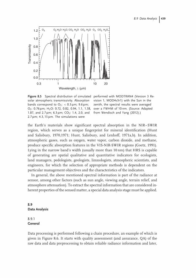
8.9 Data Analysis 439
0.3 1 10 20
1.2
1.0
0.8
0.6
0.4
0.2
0.0
Wavelength, l (μm)
Tra
nsm
issi
vity
O2O3 H2O H2O, CO2 CO2H2O O3CO2H2O H2O
Figure 8.5 Spectral distribution of simulatedsolar atmospheric transmissivity. Absorptionbands correspond to O3: < 0.3 μm; 9.6 μm;O2: 0.76 μm; H2O: 0.72, 0.82, 0.94, 1.1, 1.38,1.87, and 2.7 μm; 6.3 μm; CO2: 1.4, 2.0, and2.7 μm; 4.3, 15 μm. The simulations were
performed with MODTRAN4 (Version 3 Re-vision 1, MOD4v3r1) with the Sun in thezenith, the spectral results were averagedover a FWHM of 10 nm. (Source: Adaptedfrom Wendisch and Yang (2012).)
the Earth’s materials show significant spectral absorption in the NIR–SWIRregion, which serves as a unique fingerprint for mineral identification (Huntand Salisbury, 1970,1971; Hunt, Salisbury, and Lenhoff, 1971a,b). In addition,atmospheric gases, such as oxygen, water vapor, carbon dioxide, and methane,produce specific absorption features in the VIS-NIR-SWIR regions (Goetz, 1991).Lying in the narrow band’s width (usually more than 10 nm) that HRS is capableof generating are spatial qualitative and quantitative indicators for ecologists,land managers, pedologists, geologists, limnologists, atmospheric scientists, andengineers, for which the selection of appropriate methods is dependent on theparticular management objectives and the characteristics of the indicators.
In general, the above mentioned spectral information is part of the radiance atsensor, among other factors (such as sun angle, viewing angle, terrain relief, andatmosphere attenuation). To extract the spectral information that are considered in-herent properties of the sensed matter, a special data analysis stage must be applied.
8.9Data Analysis
8.9.1General
Data processing is performed following a chain procedure, an example of which isgiven in Figure 8.6. It starts with quality assessment (and assurance, QA) of theraw data and data preprocessing to obtain reliable radiance information and later,
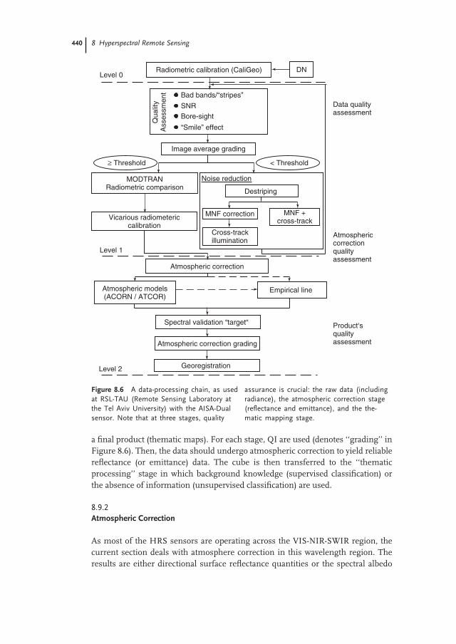
440 8 Hyperspectral Remote Sensing
MODTRANRadiometric comparison
Noise reduction
< Threshold
Radiometric calibration (CaliGeo) DN
Qua
lity
Ass
essm
ent Bad bands/“stripes”
SNRBore-sight
“Smile” effect
Image average grading
≥ Threshold
Destriping
Vicarious radiometericcalibration
MNF correction MNF +cross-track
Cross-trackillumination
Level 0
Level 1
Level 2
Atmospheric correction
Atmospheric models(ACORN / ATCOR)
Empirical line
Spectral validation “target“
Atmospheric correction grading
Georegistration
Data qualityassessment
Atmosphericcorrectionqualityassessment
Product‘squalityassessment
Figure 8.6 A data-processing chain, as usedat RSL-TAU (Remote Sensing Laboratory atthe Tel Aviv University) with the AISA-Dualsensor. Note that at three stages, quality
assurance is crucial: the raw data (includingradiance), the atmospheric correction stage(reflectance and emittance), and the the-matic mapping stage.
a final product (thematic maps). For each stage, QI are used (denotes ‘‘grading’’ inFigure 8.6). Then, the data should undergo atmospheric correction to yield reliablereflectance (or emittance) data. The cube is then transferred to the ‘‘thematicprocessing’’ stage in which background knowledge (supervised classification) orthe absence of information (unsupervised classification) are used.
8.9.2Atmospheric Correction
As most of the HRS sensors are operating across the VIS-NIR-SWIR region, thecurrent section deals with atmosphere correction in this wavelength region. Theresults are either directional surface reflectance quantities or the spectral albedo

8.9 Data Analysis 441
values (Nicodemus et al. 1977). Note, we use the term ‘‘reflectance’’ hereafter as ageneric term of a relation between reflected and incoming radiative flux (Eq. (8.2)).This radiometric conversion of the measured radiance to reflectance is referredto as ‘‘atmospheric correction’’ already in early remote sensing literature (Dozierand Frew, 1981). Note that the term ‘‘correction’’ is appropriate as long as dataare adjusted to match a given ground reference by empirical methods. However,it may be misleading for methods relying on physical radiative transfer models.The term ‘‘atmospheric compensation’’ would be a more appropriate descriptionin this case, as the atmospheric effects are compensated from correctly calibratedimagery; however, this term has not yet been widely established.
In this section, some empirical normalization methods are summarized first,which allow for fast and efficient atmospheric correction. The basics of methodsbased on radiative transfer models are given in the subsequent subsections.
8.9.2.1 Empirical Reflectance NormalizationAll empirical atmospheric correction methods have in common that a prioriknowledge about the surface spectral albedo is put in relation to the imagery inorder to find factors for a normalization of the atmospheric effect (Smith et al.1987). Hereafter, a collection of methods that are suited for systems of unsecuredcalibration state and if fast results are required are compiled. These methods maybe applied on uncalibrated image data, that is, directly on the digital number DNs.
The flat-field approach (Dobbins and Boone, 1998) uses a spectrally flat spectrumfrom within the image for normalization to calculate a flat-field (quasi-) reflectanceρff such that
ρff = DNs
DNff(8.8)
where DNs is the (uncalibrated) digital number signal at the sensor and DNff is thesignal of a selected spectrum. This normalization may result in reflectance valuesabove 100% as the selected flat-field reflectance is usually below 100 %.
The known/bright target approach uses the known (or assumed) reflectance ρb
of one typically bright target in the image such that the whole (calibrated) imagedata may be normalized by the at-sensor measurement DNb at the target by thetransformation:
ρ = DNs
DNb· ρb (8.9)
A variation of the bright target approach is the ‘‘quick atmospheric correction’’(QUAC) method (Bernstein et al. 2008). Instead of taking one pixel as a reference,the relation of a generic expected average reflectance to the average signal in theimage is taken as reference for correction of the full image, also known as IARRmethod (Kruse, 1988).
The empirical line correction uses a combination between dark and bright targetsin a scene. If two or more objects are known, a linear function is derived for eachspectral band between measured signal and reflectance. The linear fit is performedbetween the known reflectances ρi and the respective measurements DNi, such
442 8 Hyperspectral Remote Sensing
that a slope �ρ/�DN of the function ρ(DN) with a typical offset for dark objectsDNdark can be found. This function is then used for normalization of all spectra ofthe image using the equation
ρ = (DNs − DNdark) · �ρ
�DN(8.10)
The empirical line works satisfactorily well for flat terrain and small FOV imagerybut is at its limit in mountainous areas and if repeatable corrections are requiredfor an image series.
8.9.2.2 At-Sensor Radiance DescriptionOther than the empirical correction methods, the physical atmospheric correctionof HRS data relies on an appropriate description of the at-sensor radiance fromknown parameters. In HRS, the at-sensor radiance is composed of three majorcomponents comprising the direct reflected and the backscattered radiance fromthe surface and the atmosphere. The thermal emission may be neglected for thewavelength range up to 2.50 μm as long as the temperature of the surface is below350 K. Thus, the at-sensor radiance Is may be in a good approximation described asa sum of the direct ground-reflected radiance Ig,dir, the so-called adjacency radianceIg,adj, and the atmospheric radiance Iatm:
Is = Ig,dir + Ig,adj + Iatm (8.11)
We use ρ as the in-field hemispherical–directional reflectance factor (alsodenoted as HDRFmeas), ρadj as the large-scale spectral albedo of the surface, ands as the spherical albedo of the atmosphere. The terms in Eq. (8.11) may then bewritten in a good approximation for the direct component
Ig,dir = 1
π· Fg · ρg · τu (8.12)
the adjacency radiance
Ig,adj = 1
π· Fg · ρadj · τu,adj (8.13)
and the atmospheric radiance
Iatm = 1
π· F0 · s (8.14)
The term F0 is the top-of-atmosphere irradiance and Fg is the total irradiance (solarflux) on a ground surface element, which may be written as
Fg = F0 · τd · cos ϕ + Fdif · Vsky + Fter (8.15)
The latter depends on the local solar incidence angle ϕ and includes the totaldiffuse irradiance Fdif , scaled by the fraction of the visible sky (skyview factor Vsky)and the terrain irradiance Fter. The parameter τd is the downward atmospherictransmittance; τu and τu,adj are the upward transmittances of the atmosphere forthe direct and the adjacency radiative paths, respectively.
8.9 Data Analysis 443
A different formulation of the at-sensor radiance is derived, if the adjacencyterm is written using the back-reflected radiance from the ground coupled by thesingle scattering albedo s of the atmosphere, compare (Tanre et al. 1979). Here,all ground-reflected radiance is summarized in the term Ig,tot. This results in thefollowing relation:
Is = Ig,tot + Iatm = τu · Fg · ρg · 1
π · (1 − ρadj · s)+ Iatm (8.16)
where the parameters are as described for Eq. (8.11). Such formulations of theat-sensor radiance are the basis for the atmospheric correction task.
8.9.2.3 Radiative-Transfer-Based Atmospheric CorrectionRadiative transfer codes (RTCs) such as MODTRAN®-5 (Berk et al. 2005) or6 S-V (Vermote et al. 2006) are well suited for forward simulation of the at-sensorsignal from given boundary conditions. However, they are not built for the taskof inversion for surface reflectance properties from radiometric images. For thispurpose, atmospheric correction software is required. Examples of such software areTAFKAA (Gao et al. 2000), ACORN (Atmospheric Correction Now) (Green, 2001),HAATCH (High Accuracy Atmospheric Correction for HRS Data) (Qu, Goetz, andHeidbrecht, 2001), ATCOR (Atmospheric Topographic Correction) (Richter andSchlapfer, 2002), or FLAASH (Fast Line-of-Sight Atmospheric Analysis of SpectralHypercubes) (Cooley et al. 2002). Such software allows an efficient inversion ofthe calibrated imagery on the basis of set of equations bellow. By inversion andreformulation of Eq. (8.11), the surface reflectance may be retrieved by the followingequation:
ρg = π · d2 · (Is − Ig,adj − Iatm
)
τu · (τd · F0 cos ϕ + Fdif · Vsky + Fter
) (8.17)
The components of this equation are to be derived from (i) physical model ofa radiative transfer code: Iatm, Fdif , τd, and τu; (ii) boundary conditions of terrain:incidence angle ϕ and sky view factor Vsky; (iii) astronomical data: the averageextraterrestrial solar constant F0 and the dependency on the relative Earth–Sundistance described by parameter d; and (iv) iteration of atmospheric correction:Ig,adj and terrain irradiance Fter.
As all the parameters except F0 and d vary per pixel, it is not feasible to calculatethe radiative transfer directly for each pixel. Precalculated look-up tables (LUTs) arenormally employed. These LUTs are interpolated with the pixel properties to findthe applicable parameters for the correction.
A different approach is to perform the atmospheric compensation in the ‘‘ap-parent reflectance’’ domain ρs after dividing the at-sensor radiance by the ground

444 8 Hyperspectral Remote Sensing
solar irradiance, propagated to the at-sensor level F0,s:
ρs = π · d2 · Is
F0,s(8.18)
ρatm = π · d2 · Iatm
F0,s(8.19)
ρadj = π · d2 · Iadj
F0,s(8.20)
These terms are typically used over flat ground, introducing a total transmittanceterm τtot = τd · τu, which relates the at-sensor reflectance to the ground reflectance.The inversion of Eq. (8.16) for reflectance results in
ρg = (ρs − ρatm) · (1 − ρadj · s
)
τtot(8.21)
If the adjacency reflectance is further assumed to be the same as the pixel reflectance(i.e., ρadj = ρg), the equation is reduced to
ρg = (ρs − ρatm)
τtot + (ρs − ρatm) · s(8.22)
This is a basic atmospheric correction equation, which may be used in simpleatmospheric correction programs or for fast inversion of a radiative transfer code.Note that working in the reflectance domain is critical for airborne instruments,as this approximation relies on accurate knowledge of the radiance at sensor level.An additional modeling step is required to infer the at-sensor radiance level F0,s asa reference value.
8.9.3Process of Complete Atmospheric Correction
A complete atmospheric correction as implemented in atmospheric correctionroutines follows these steps: (i) create a LUT, containing the parameters of theabove equations in relation to the parameters at a fixed number of data points(covering the expected range); (ii) calculate skyview factor, height, and incidenceangle from DEM (digital elevation model), using the solar zenith and azimuthangles; (iii) derive atmospheric parameters from imagery (i.e., water vapor andaerosol load of the atmosphere); (iv) make fixed preselections (e.g., flight altitudeand aerosol model); (v) invert the LUT, that is, derive the parameters by multilinearinterpolation for each pixel; (vi) use Eq. (8.10) or (8.22) to perform the atmosphericcorrection; and (vii) perform the last two iteration of steps for adjacency correctionand for the calculation of the terrain irradiance.
Some variations of this procedure exist, as the parameterization of the problemmay differ and the LUT may be precalculated or calculated for each scene directlywhile correcting the data. An ideal high level standard procedure combines geomet-ric and atmospheric processing (Schlapfer and Richter, 2002). Linked parametersare the viewing angle per pixel, the absolute distance from the aircraft to each
8.9 Data Analysis 445
pixel location, or the relative air mass between sensor and pixel. Furthermore,other DEM related parameters, such as height, slope, or aspect, are required forradiometric correction algorithms and can only be used if the image is broughtto the same geometry as the DEM. The dependencies within the atmosphericcorrection part lead to iterative reflectance retrieval steps, specifically for adjacencycorrection purposes. The final step of the processing should be a correction ofthe reflectance anisotropy (i.e., a BRDF correction). Some details regarding crucialcorrection steps are given hereafter.
8.9.3.1 Atmospheric Parameter RetrievalAirborne HRS sensors offer the inherent capability for automatic retrieval of theradiometrically critical parameters atmospheric water vapor content and aerosolload (optical thickness). For the atmospheric water vapor, the 0.94/1.13 μm watervapor absorption bands are typically used for the retrieval of columnar water vaporover land on a per-pixel basis (Schlapfer et al. 1998). The aerosol optical thicknessis normally calculated using the dark dense vegetation (DDV) approach (Kaufmanand Tanre, 1996) interpolating the aerosol load to areas not covered by vegetation.These two methods allow for a mostly autonomous atmospheric correction of HRSdata.
8.9.3.2 Adjacency CorrectionThe correction of the atmospheric adjacency effect is of high relevance, especially forlimnological applications (Tanre et al. 1987). The effect is significant in a horizontalrange from 100 m up to 1.5 km starting at flight altitudes of 1000 m above groundand higher. Thus, each pixel has to be corrected with respect to the averagereflectance of the adjacent areas. This can be carried out in an efficient way by thedefinition of a spatial convolution function, which takes a distance-weighted averageof the adjacent area in the image to calculate an adjacency weighting factor. Thecorresponding radiance has to be simulated in the radiative transfer code as indirectground-reflected radiance according to the aforementioned parameterization.
8.9.3.3 Shadow CorrectionCast shadows, cloud shadows, and shadows from building are often present in HRSdata. They receive mostly diffuse irradiance that is sufficient to provide enoughsignal for data analysis with state of the art sensor systems. Correction approachestry to classify the shadowed areas first and then apply a separate correction modelto these parts of the image such that shadows are removed in optimal situations(Adler-Golden et al. 2002; Richter and Muller, 2005). The correction model takesinto account the diffuse nature of the irradiance in the cast shadow areas and needsto consider the skyview factors correctly for an accurate correction.
8.9.3.4 BRDF CorrectionThe derivation of spectral albedo (i.e., the bihemispherical reflectance, BHR) fromdirectional reflectance values is the task of BRDF correction. The operationalcorrection of BRDF effects in images is not yet solved satisfactorily, but progress
446 8 Hyperspectral Remote Sensing
has been made on this issue (Feingersh, Ben-Dor, and Filin, 2010). The correctionof the BRDF effects may be performed if the BRDF properties of the observedtarget(s) and the (diffuse) irradiance distribution is known. For operational use,an anisotropy factor needs to be calculated and applied for each pixel. This factoraccounts for the relation between measured hemispherical–directional reflectance(HDRFmeas) and the spectral albedo (BHR; also known as white sky albedo). Theanisotropy factor has to be inferred from an appropriate BRDF model or frommeasurements. The finally calculated spectral albedo product is a quantity that maybe easily compared in multitemporal analysis and may be used for unbiased objectclassification.
8.9.4Retrieval of Atmospheric Parameters
On the basis of the relatively high spectral resolution obtain by the HRS sensors,one can use the specific absorption features of atmospheric gases (natural orcontaminated) and evaluate their column content on a pixel-by-pixel basis. Thismay provide an innovative way of mapping the gases’ spatial distribution andof spotting new quantitative information on the atmospheric conditions at veryhigh spatial resolution. The gases that are active across the UV-VIS-NIR-SWIR-TIRspectra are divided into two sectors: (i) a major sector in which the spectral responseof the gases is well detected (high fraction and strong absorption) and (ii) a minorsector in which the spectral response is low and difficult to assess because of thelow fraction of the gases and relatively weak absorption features. The major gasgroup is composed of O2, H2O, and CO2, whereas the minor gas group consistsof O3, N2O, CO, and CH3 in the UV-VIS-NIR-SWIR and SO2 and NO2 in theTIR. Figure 8.7 provides the absorptance features of the above gas componentsacross the UV-VIS-NIR-SWIR-TIR spectral region along with the atmosphericwindows. The advantage of assessing the above gases on a pixel-by-pixel basisis significant. It can help accurately extract surface reflectance by estimating thegases’ absorption (and hence their atmospheric transmission) on a pixel-by-pixelcolumn basis. Consequently, calculating water vapor directly from the image, firstdemonstrated by Gao and Goetz (1995), is now a very common way of achievinghigh performance of atmospheric correction methods (Section 8.8). While H2O isconsidered to be a nonuniformly spatially distributed gas, other major gases, thatis, CO2 and O2, are known to be well mixed – hence, their use as indicators toassess atmospheric phenomena that might affect the spatial distribution of the gasin question. For example, over rough terrain, if spatial changes are encounteredusing a well-mixed gas, this might indicate different elevations, as the column pixelvolume over high terrain consists of less molecules than that over low terrains fora particular gas. On the basis of this, Ben-Dor and Kruse (1996) and Green (2001)showed that it is possible to construct a DEM structure of the studied area solelyfrom the HRS radiance information and the CO2 peak. Furthermore, as O2 isalso a well-mixed gas, it can be used to estimate, on a pixel-by-pixel basis, the Miescattering effect across the VIS–NIR region and hence can be used to better extract
8.9 Data Analysis 447
the surface reflectance, assuming that the scattering is not a spatially homogeneousphenomenon. Using one absorption peak of the H2O at 1.38 μm, Gao, Goetz, andWiscombe (1993) showed that a nonvisible cirrus cloud can be detected and mappedbased on the high scattering properties of the ice particles within the cloud volume.Ben-Dor (1994) suggested taking precautions in using these absorption peaks overhigh terrain and bright targets, and in another paper, (Ben-Dor, Goetz, and Shapiro,1994) suggested that the O2 peak be used to map the cirrus cloud distribution inthe VIS–NIR region (0.760 μm). On the basis of this idea, Schlapfer et al. (2006)was able to quantitatively assess a smoke plume over a fire area using the scatteringeffect on the O2 absorption peak. Alakian, Marion, and Briottet (2008) developeda method to retrieve the microphysical and optical properties in aerosol plumes(L-APOM) in the VIS region as well. Recently, Chudnovsky et al. (2009) mapped adust plume over the Bodele depression in northern Chad using Hyperion data andthe SWIR region. Another innovative study that shows the applicability of HRSin the atmosphere was performed by Roberts et al. (2010). They showed that ifhigh SNR data are available, it is also possible to detect the distribution of minorgases. Using AVIRIS 2006 data over a marine (dark) environment, they were ableto detect, on a pixel-by-pixel basis, the emission of methane over the Coal Oil Point(COP) marine seep fields, offshore of Santa Barbara, California, and the La BreaTar Pits in Los Angeles, California. In the TIR region, there are several examplesof the detection of plumes of toxic gases based on the fundamental vibration peakacross the atmospheric windows between 2.5 and 16 μm. Using SO2 emission inthe LWIR region at 8.58 and 8.82 μm, Shimoni et al. (2007) were able to spot shadeon a plume emitted over an industry refinery zone with additional informationextracted from the VIS region. Figure 8.7 provides a summary for the absorptionpositions of some of the above mentioned gases across the VIS-NIR-SWIR-TIRspectral region. In summary, it can be concluded that HRS technology is not onlycapable of deriving surface information but also has the proven capability to extractquantitative information on atmosphere constituents in an innovative way thatnone of the current remote sensing means can provide.
8.9.5Mapping Methods and Approaches
Over the past few years, many techniques for mapping and processing of HRSdata have been developed (Schaepman et al. 2009). The special characteristics ofhyperspectral data sets pose different processing problems, which must be tackledunder specific mathematical formulations, such as classification (Landgrebe, 2003;Richards and Jia, 2006) or spectral unmixing (Adams, Smith, and Johnson, 1986).These problems also require specific dedicated processing software and hardwareplatforms (Plaza and Chang, 2007).
In previous studies (Plaza et al. 2009), available techniques were divided intofull-pixel and mixed-pixel techniques, where each pixel vector defines a spectralsignature or fingerprint that uniquely characterizes the underlying materials ateach site in a scene. Mostly based on previous efforts in multispectral imaging,
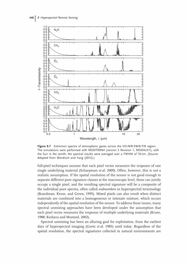
448 8 Hyperspectral Remote Sensing
0.3 1 10 20
Wavelength, l (μm)
O2
O3
H2O
CO2
1.00.80.60.40.20.0
1–T
rans
mis
sivi
ty
N2O
CH4
1.00.80.60.40.20.01.00.80.60.40.20.01.00.80.60.40.20.01.00.80.60.40.20.01.00.80.60.40.20.01.00.80.60.40.20.0
Figure 8.7 Extinction spectra of atmospheric gases across the VIS-NIR-SWIR-TIR region.The simulations were performed with MODTRAN4 (version 3 Revision 1, MOD4v3r1), withthe Sun in the zenith; the spectral results were averaged over a FWHM of 10 nm. (Source:Adapted from Wendisch and Yang (2012).)
full-pixel techniques assume that each pixel vector measures the response of onesingle underlying material (Schaepman et al. 2009). Often, however, this is not arealistic assumption. If the spatial resolution of the sensor is not good enough toseparate different pure signature classes at the macroscopic level, these can jointlyoccupy a single pixel, and the resulting spectral signature will be a composite ofthe individual pure spectra, often called endmembers in hyperspectral terminology(Boardman, Kruse, and Green, 1995). Mixed pixels can also result when distinctmaterials are combined into a homogeneous or intimate mixture, which occursindependently of the spatial resolution of the sensor. To address these issues, manyspectral unmixing approaches have been developed under the assumption thateach pixel vector measures the response of multiple underlying materials (Kruse,1988; Keshava and Mustard, 2002).
Spectral unmixing has been an alluring goal for exploitation, from the earliestdays of hyperspectral imaging (Goetz et al. 1985) until today. Regardless of thespatial resolution, the spectral signatures collected in natural environments are
8.9 Data Analysis 449
invariably a mixture of the signatures of the various materials found within thespatial extent of the ground instantaneous field view of the imaging instrument(Adams, Smith, and Johnson, 1986). In this case, the measured spectrum may bedecomposed into a combination of pure spectral signatures of soil and vegetation,weighted by areal coefficients that indicate the proportion of each macroscopicallypure signature in the mixed pixel (Keshava and Mustard, 2002). The availability ofhyperspectral imagers with a number of spectral bands exceeding the number ofspectral mixture components (Green et al. 1998) has allowed casting the unmixingproblem in terms of an over determined system of equations in which, given a setof pure spectral signatures (called endmembers), the actual unmixing to determineapparent pixel abundance fractions can be defined in terms of a numerical inversionprocess (Harsanyi and Chang, 1994; Bateson and Curtiss, 1996; Plaza et al. 2004;Berman et al. 2004; Chang et al. 2006; Rogge et al. 2006; Wang and Chang, 2006;Zaer and Gader, 2008).
A standard technique for spectral mixture analysis is linear spectral unmixing(Heinz and Chang, 2001; Plaza et al. 2004), which assumes that the spectracollected by the spectrometer can be expressed in the form of a linear combinationof endmembers weighted by their corresponding abundances. It should be notedthat the linear mixture model assumes minimal secondary reflections and multiplescattering effects in the data-collection procedure, and hence, the measured spectracan be expressed as a linear combination of the spectral signatures of materialspresent in the mixed pixel (Figure 8.8a). Although the linear model has practicaladvantages, such as ease of implementation and flexibility in different applications(Chang, 2003), nonlinear spectral unmixing may best characterize the resultantmixed spectra for certain endmember distributions, such as those in which theendmember components are randomly distributed throughout the instrument’sFOV (Guilfoyle, Althouse, and Chang, 2001). In those cases, the mixed spectracollected by the imaging instrument are better described by assuming that partof the source radiation is multiply scattered before being collected at the sensor(Figure 8.8b). In addition, several machine-learning techniques have been appliedto extract relevant information from hyperspectral data during the past decade.Taxonomies of remote sensing data-processing algorithms (including hyperspectralanalysis methods) have been developed in the literature (Richards and Jia, 2006Schowengerdt, 1997). It should be noted, however, that most available hyperspectraldata-processing techniques focus on analyzing the data without incorporatinginformation on the spatially adjacent data, that is, hyperspectral data are usuallynot treated as images but as unordered listings of spectral measurements with noparticular spatial arrangement (Rogge et al. 2006). The importance of analyzingspatial and spectral patterns simultaneously has been identified as a desired goalby many scientists devoted to multidimensional data analysis.
In certain applications, however, the integration of high spatial and spectralresolution is mandatory to achieve sufficiently accurate mapping and detectionresults. For instance, urban area mapping requires sufficient spatial resolutionto distinguish small spectral classes, such as trees in a park or cars on a street(Bruzzone and Marconcini, 2006). Owing to the small number of training samples
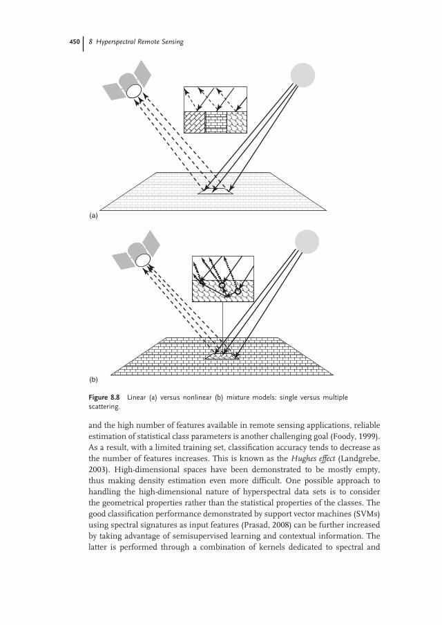
450 8 Hyperspectral Remote Sensing
(b)
(a)
Figure 8.8 Linear (a) versus nonlinear (b) mixture models: single versus multiplescattering.
and the high number of features available in remote sensing applications, reliableestimation of statistical class parameters is another challenging goal (Foody, 1999).As a result, with a limited training set, classification accuracy tends to decrease asthe number of features increases. This is known as the Hughes effect (Landgrebe,2003). High-dimensional spaces have been demonstrated to be mostly empty,thus making density estimation even more difficult. One possible approach tohandling the high-dimensional nature of hyperspectral data sets is to considerthe geometrical properties rather than the statistical properties of the classes. Thegood classification performance demonstrated by support vector machines (SVMs)using spectral signatures as input features (Prasad, 2008) can be further increasedby taking advantage of semisupervised learning and contextual information. Thelatter is performed through a combination of kernels dedicated to spectral and
8.10 Sensor Calibration 451
contextual information, while in the former, the learning is provided with somesupervised information in addition to the wealth of unlabeled data. Among thegreat many methods proposed in the literature for such approaches, we focus on thetransductive SVM for semisupervised learning (Bruzzone and Marconcini, 2006)or a composite kernel-based methodology for contextual information integration atthe kernel level (Camps-Valls et al. 2006) have shown great success in practice.
As most of the methods reviewed here deal with endmember extraction anddata mining from the reflectance or emittance cubes (an unsupervised approach),there are methods in which the endmembers are known in advance or the spectralmodel to map the pixels has already been developed (supervised approach). Oneof the first and most usable endmember-based approaches in HRS is the SpectralAngle Mapper (SAM), developed by Kruse et al. (1993), which is based on the anglecalculated between two spectral vectors: the pixel and the selected endmember.Since then, many other spectral-based techniques have been developed, where mostrecently, spectral-based models that are generated in a spectral domain (e.g., PLSor neural network) are implemented on a pixel-by-pixel basis to the image cube inquestion. This method enables quantitative mapping of selected properties on theEarth’s surface such as infiltration rate (Ben-Dor et al. 2004) organic matter content(Stevens et al. 2008), salinity (Ben-Dor et al. 2002), and more.
Finally, although the mapping and classification techniques described abovehold great promise for hyperspectral data processing, they also introduce newcomputational challenges. With the recent explosion in the amount and complexityof hyperspectral data, parallel processing and high-performance computing (HPC)practices have necessarily become requirements in many remote sensing missions,especially with the advent of low-cost systems such as commodity clusters (Plazaand Chang, 2007). On the other hand, although hyperspectral analysis algorithmsmap nicely to clusters and networks of workstations, these systems are generallyexpensive and difficult to adapt to on-board data-processing requirements intro-duced by several applications, such as wildland fire tracking, biological threatdetection, monitoring of oil spills, and other types of chemical contamination.In those cases, low-weight and low-power integrated components are essential toreducing the mission’s payload and obtaining analyzed results quickly enough forpractical use. In this regard, the emergence of specialized hardware devices suchas field-programmable gate arrays (FPGAs) has helped in bridging the gap towardreal-time analysis of remotely sensed hyperspectral data.
8.10Sensor Calibration
8.10.1General
In combination, calibration and validation (cal/val) can be regarded as a singleprocess that encompasses the entire remote sensing system, from sensor to data
452 8 Hyperspectral Remote Sensing
product. The objective of both is to develop a quantitative understanding andcharacterization of the measurement system and its biases in both space and time(National Research Council, 2007). Calibration of hyperspectral sensor data is acritical activity for a number of reasons. First, we need to have confidence in thereliability of data delivered by such sensors. Second, as many of the products thatwe are deriving from hyperspectral data are quantitative, we need to know thatthe data from which they are derived are accurate (this holds for qualitative dataas well). We often test the accuracy of remote sensing data products by performingvalidation of the subsequent data sets; thus, the raw data delivered by sensorsmust be well calibrated and the products derived from them are also well validated.cal/val are, therefore, activities that form an integral component of the efficientuse of any form of EO data and in the maintenance of the scientific value of EOdata archives. As HRS data are acquired in DN values, but for most applications,we need radiometric information as an input to extract reflectance or emissivityvalues, accurate transfer from one stage to another is crucial. In this respect,radiometric and spectroscopic assurance is required. Radiometric calibration refersto the process of extracting physical units from the original raw spectroscopic dataand assigning the channels in the sensors to a meaningful wavelength.
Cal/val is, therefore, a fundamentally important scientific activity and should bea continuous component in any remote sensing program, providing an indepen-dent check on the performance of both space-based airborne and ground-basedhyperspectral sensors and processing algorithms.
In general, one can say that the calibration of EO data is critical if we areto reliably attribute detected changes observed in data to real environmentalchanges occurring at ground level. Without calibration, we are unable to ruleout the influence of other factors, such as instrument error or influences ofthe atmosphere. This problem is exacerbated by the myriad of sensors operatedby multiple countries and organizations. Calibration allows the traceability ofsensor data to the same physical standards and is routinely required as sensorsdecay throughout their lifetime. Calibration is thus critical if we want to reliablyextract information from measured radiance, compare information acquired fromdifferent regions and different times, compare and analyze HRS observationswith measurements provided by other instruments, and extract information fromspectral image measurements using physically based computer models.
Validation refers to the independent verification of the physical measurementsmade by a sensor as well as the derived geophysical variables. Validation allowsfor the verification and improvement of the algorithms used (e.g., for atmosphericcorrection and vegetation state). To achieve this, conventional, ground-based ob-servations are required using calibrated and traceable field instrumentation andassociated methods. To this end, several indicators are valid and developed to checkthe accuracy of the calibration stage and provide the user with a reliable feelingabout his data set.
The definition of all the common terms used here for cal/val are taken from theCommittee of Earth Observation Satellites (CEOS) as follows:
8.10 Sensor Calibration 453
(i) Calibration. The process of quantitatively defining the responses of a systemto known, controlled signal inputs;
(ii) Validation. The process of assessing, by independent means, the quality ofthe data products derived from the system outputs;
(iii) Traceability. Property of a measurement result relating the result to a statedmetrological reference (free definition and not necessarily SI) through anunbroken chain of calibrations of a measuring system or comparisons, eachcontributing to the stated measurement uncertainty;
(iv) Uncertainty. Parameter that characterizes the dispersion of the quantity valuesthat are being attributed to a measured mean, based on the information used;
(v) Vicarious Calibration. Vicarious calibration refers to techniques that make useof natural or artificial sites on the surface of the Earth for post calibration ofairborne or spaceborne sensors.
8.10.2Calibration for HSR Sensor
Calibration translates electrical output DN values (voltages or counts) to reli-able physical-based units (radiometric information) by determining the transferfunctions and coefficients necessary to convert a sensor reading. The coeffi-cients are extracted throughout a careful measurement stage in the laboratoryusing well-calibrated facilities and traceable standards. There are a number ofcomponents ensuring a thorough calibration approach. Radiometric and spectralresponses need to be accurately monitored through the lifetime of a sensor tomonitor changes in response, as it ages over time. In the case of spacebornehyperspectral sensors, both prelaunch and post (on-orbit) launch calibrations areundertaken, either directly or using vicarious targets-on-orbit and vicarious calibra-tion enable taking into account changes in calibration over time using the moon’ssurface (Kieffera et al. 2003). Airborne hyperspectral sensors have the advantageover spaceborne sensors that they can be removed from the aircraft and resubjectedto rigorous laboratory calibration tests similar to those performed for prelaunchcalibration of spaceborne sensors. This is often performed before and after a flying‘‘season.’’ The calibration coefficients from each season can also be used to trackthe sensor’s deterioration over its years of operation.
8.10.2.1 Preflight CalibrationThe three key components to prelaunch calibration are radiometric, spectral,and spatial. Achieving radiometric calibration involves the use of a calibratedintegrating sphere whose ideal output is homogeneous and large enough toilluminate all elements in a sensor array with the same radiance. An absoluteradiometric calibration determines the relationship between sensor signals andradiance for all spectral channels. Varying the output of the integrating sphere alsoallows for the study of the linearity between sensor response and radiance andthe assessment of the SNR at radiance levels similar to those encountered whensensing the Earth’s surface (Gege et al. 2009).
454 8 Hyperspectral Remote Sensing
Spectral calibration typically uses a monochromator to produce a collimatednarrow beam of light that is blocked by transmission filters and is thus tunableto different wavelengths. Measurements performed here allow for determinationof spectral response function, center wavelength, spectral smile, spectral samplingdistance, the spectral range of pixels, and spectral resolution and to perform awavelength calibration (Oppelt and Mauser, 2007).
Spatial calibration (geometric) can most accurately be achieved with the move-ment of a point light source across the sensor array whose beam is controlled by aslit (Gege et al. 2009). This allows for along-track and across-track calibration of thesensor array. Measurements performed here allow for the derivation of line spreadfunction across track; center coordinates for each CCD in the array; across-tracksampling distance; pixel instantaneous FOV; total sensor FOV; and the modulationtransfer function (the reparability of adjacent targets as a function of distance andcontrast (Oppelt and Mauser, 2007).
8.10.2.2 In-Flight/In-Orbit CalibrationThis involves the use of in-built calibration sources and vicarious calibration orcross-calibration to other satellite sensors. The critical issue at this stage is to beable to monitor changes in sensor performance over time (Pearlman et al. 2003).For example, Hyperion, the first fully spaceborne hyperspectral sensor, relied onthe diffuse reflectance of an in-built Spectralon ™reflectance surface illuminatedby the Sun or a lamp, in calibrations performed once every two weeks. The moonand other opportunistic Earth surface targets were also used to monitor sensorperformance over time (Jarecke and Yokoyama, 2000; Pearlman et al. 2003; Ungaret al. 2009). Cross-calibration to data from the LANDSAT 7 ETM+ sensor was alsofrequently performed.
EnMAP, the new German-built hyperspectral sensor scheduled for launch in2015, will carry for calibration a full aperture diffuser, coupled with an integratingsphere with various calibration lamps. A shutter mechanism also allows for darkmeasurements to be performed. APEX, a joint Belgian–Swiss airborne sensordevelopment, carries an in-flight characterization facility using a stabilized lampcoupled with vicarious and cross-calibration (Nieke et al. 2008), (Itten et al. 2008).
8.10.2.3 Vicarious CalibrationVicarious calibration is also used as an in-flight check on sensor performance(Green and Shimada, 1997; Green and Pavri, 2000; Secker et al. 2001). The ap-proach can use homogeneous targets on the land surface (e.g., dry lake beds,desert sands, ice sheets, water bodies, and so on) or artificial targets of varyingbrightness if the sensor has sufficient spatial resolution (Brook and Ben-Dor,2011). The sites or targets must be well characterized, and ideally, reflectance and,if possible, radiance should be measured at the ground surface using calibratedspectroradiometers simultaneously with sensor overflight. Increasingly sophisti-cated ground-based instrumentation is being used to provide autonomous andnear-continuous measurement of the characteristics at many of these sites (Brandoet al. 2010). Correction involves either top-down (correction of ‘‘top-of-atmosphere’’
8.10 Sensor Calibration 455
sensor data to ground-leaving reflectance using an atmospheric correction model)or bottom-up (correction of ground target reflectance to top-of-atmosphere radi-ance using a radiative transfer model taking into account atmospheric transmissionand absorption, e.g., MODTRAN). Increasingly, a combination of measurementsobtained at varying scales and resolutions (e.g., in situ, airborne, and satellite) arebeing used to provide the basis for assessment of the on-orbit radiometric andspectral calibration characteristics of spaceborne optical sensors (Green, Pavri, andChrien, 2003a).
The smaller pixel sizes of airborne imagery compared to typical image satelliteresolutions, along with targeted deployment, means that artificial vicarious cali-bration targets can be rapidly deployed in advance of specific airborne campaigns.Such targets can also help overcome the difficulties of finding sufficient naturalhomogeneous targets of varying brightness. Supervised vicarious calibration (SVC)(Brook and Ben-Dor, 2011) uses artificial agricultural black polyethylene nets ofvarious densities as calibration targets, set up along the aircraft’s trajectory. Thedifferent density nets, when combined with other natural bright targets, can pro-vide full coverage of a sensor’s dynamic range. The key to the use of any form ofvicarious calibration target is the use of simultaneous field-based measurement oftheir reflectance properties and positions; uncertainties are reduced if a number ofcalibration targets are used, a large number of reflectance measurements are madeof each target, and their positions are accurately located (Secker et al. 2001).
Vicarious calibration, therefore, provides an indirect means of QA of remotelysensed data and sensor performance that is independent of direct calibrationmethods (use of on-board radiance sources or panels). This is important ason-board illumination sources may themselves degrade over time.
In all calibration efforts, traceability, the process of ensuring measurements, isrelated through an unbroken chain of comparisons to standards held by NationalMetrology Institutes (e.g., National Institute of Standard and Technology (NIST),USA; PTB, National Standards Laboratory, Germany; and National Physics Labo-ratory (NPL), UK), is the key to allowing true intercomparability between differentsensors’ raw and product data sets (Fox, 2004). The chain is implemented via the useof ‘‘transfer standards’’ that allow traceability back to official ‘‘primary’’ radiometricstandards using internationally agreed-upon systems of units (SI) and rigorousmeasurement and test protocols. Integral to the establishment of traceability isthe quantification and documentation of associated uncertainties throughout themeasurement chain; the fewer the number of steps in the chain, the lower the un-certainty. The advantages of maintaining traceability include a common referencebase and quantitative measures of assessing the agreement of results for differentsensors or measurements at different times. However, current traceability guide-lines lack guidance on temporal overlap or interval length for the measurementsin the unbroken chain of comparisons (Johnson, Rice, and Brown, 2004).
The successful implementation of cal/val activity needs careful planning ofissues such as coordination of activities, selection and establishment of net-works of sites, the development and deployment of instrumentation to support
456 8 Hyperspectral Remote Sensing
measurement campaigns, the adoption of common measurement, and data distri-bution/availability protocols.
8.11Summary and Conclusion
This chapter provides a snapshot of the emerging HRS technology. Althoughmany aspects of this promising technique are not covered herein, we hope to haveprovided the reader with a sense of its potential for the future, as evidenced by pastaccomplishments. Besides being a technology that can provide added value to theremote sensing arena, it is an expansion of the spectroscopy discipline that hasbeen significantly developing worldwide for many years. Very soon, when sensorsin air and orbit domains begin to provide SNR values that are similar to thoseacquired in the laboratory, all spectral techniques available today will be able toimplement the HRS data and forward the applications in a generation or two.HRS technology is emerging and the general scientific community use is growing.The number of sensors is also on the rise and new companies are entering intocommercial activities. The most important step in the processing of HRS data is toobtain accurate reflectance or emissivity information on every pixel in the image; atthat point, a sophisticated analytical approach can be used. This means that besidesthe atmospheric correction method, the data has to be physically reliable andstable at the sensor level. Mixed-pixel analysis and spectral models to account forspecific questions are only a few examples of what this technology can achieve. Theforthcoming HRS sensors in orbit are expected to drive this technology forwardby providing temporal coverage of the globe at low cost and showing decisionmakers that the technology can add much to other space missions. The growingsensor-development activity in the market will also permit a ‘‘sensor for all,’’ whichwill also push the technology forward. As many limitations still exist, such as theTIR region not being fully covered, the information only being obtainable from avery thin layer, the time investment, high cost of data processing, and great effortneeded to obtain a final product, investment in this technology is worthwhile. Ifthe above limitations can be overcome, and other sensors’ capabilities merged withit, then HRS technology can be the vehicle to real success, moving from a scientificdemonstration technology to a practical commercial tool for remote sensing of theEarth.