8 Highway capacity.pdf

8/14/2019 8 Highway capacity.pdf

http://slidepdf.com/reader/full/8-highway-capacitypdf 1/18

8.1

CHAPTER 8HIGHWAY CAPACITY

Lily Elefteriadou Department of Civil Engineering,The Pennsylvania State University,University Park, Pennsylvania

8.1 INTRODUCTION

How much trafc can a facility carry? This is one of the fundamental questions designersand trafc engineers have been asking since highways have been constructed. The term‘‘capacity’’ has been used to quantify the trafc-carrying ability of transportation facilities.The value of capacity is used when designing or rehabilitating highway facilities, to obtaindesign elements such as the required number of lanes. It is also used in evaluating whetheran existing facility can handle the trafc demand expected in the future.

The denition and value for highway capacity have evolved over time. The Highway

Capacity Manual ( HCM 2000 ) is the publication most often used to estimate capacity. Thecurrent version of the HCM denes the capacity of a facility as ‘‘the maximum hourly rateat which persons or vehicles reasonably can be expected to traverse a point or a uniformsection of a lane or roadway during a given time period, under prevailing roadway, trafcand control conditions’’ ( HCM 2000, 2-2). Specic values for capacity are given for varioustypes of facilities. For example, for freeway facilities capacity values are given as 2,250passenger cars per hour per lane (pc/hr/ln) for freeways with free-ow speeds of 55 milesper hour (mph), and 2,400 pc/hr/ln when the free-ow speed is 75 mph (ideal geometricand trafc conditions).

For a long time, trafc engineers have recognized the inadequacy and impracticality of the capacity denition. First, the expression ‘‘maximum . . . that can reasonably be expected’’is not specic enough for obtaining an estimate of capacity from eld data. Secondly, eld

data-collection efforts have shown that the maximum ow at a given facility varies from dayto day, therefore a single value of capacity does not reect real-world observations.The main objective of this chapter is to provide transportation professionals with an

understanding of highway capacity and the factors that affect it, and to provide guidance onobtaining and using eld values of capacity. The next part of this chapter discusses thehistory and evolution of capacity estimation. The third part discusses the factors that affectcapacity. The fourth part presents uninterrupted ow capacity issues, while the fth partpresents interrupted ow capacity issues. The last part presents a vision for the future of dening and estimating capacity.

Downloaded from Digital Engineering Library @ McGraw-Hill (www.digitalengineeringlibrary.com)Copyright © 2004 The McGraw-Hill Companies. All rights reserved.

Any use is subject to the Terms of Use as given at the website.

Source: HANDBOOK OF TRANSPORTATION ENGINEERING



8.2 CHAPTER EIGHT

8.2 CAPACITY DEFINITION AND ESTIMATION METHODS

8.2.1 The Highway Capacity Manual —A Historical Perspective

The Highway Capacity Manual is the publication most often used to estimate capacity. Therst edition of the Highway Capacity Manual (1950) dened three levels of roadway capac-ity: basic capacity, possible capacity and practical capacity. Basic capacity was dened as‘‘the maximum number of passenger cars that can pass a point on a lane or roadway duringone hour under the most nearly ideal roadway and trafc conditions which can possibly beattained.’’ Possible capacity was ‘‘the maximum number of vehicles that can pass a givenpoint on a lane or roadway during one hour, under prevailing roadway and trafc conditions.’’Practical capacity was a lower volume chosen ‘‘without the trafc density being so great asto cause unreasonable delay, hazard, or restriction to the drivers’ freedom to maneuver underprevailing roadway and trafc conditions.’’

The second edition of the Highway Capacity Manual (1965) dened a single capacity,similarly to the ‘‘possible capacity’’ of the HCM 1950. ‘‘Basic capacity’’ was replaced by‘‘capacity under ideal conditions,’’ while ‘‘practical capacity’’ was replaced by a series of ‘‘service volumes’’ to represent trafc operations at various levels of service. It is interestingto note that in the HCM 1965, the second chapter is titled ‘‘Denitions’’ and begins asfollows: ‘‘The confusion that has existed regarding the meaning and shades of meaning of many terms . . . has contributed . . . to the wide differences of opinion regarding the capacityof various highway facilities. . . . In fact, the term which is perhaps the most widely mis-understood and improperly used . . . is the word ‘capacity’ itself.’’ Thus, the denition of the term ‘‘capacity’’ allowed for various interpretations by different trafc analysts, and therewas a desire to clarify the term. In the HCM 1965, the denition of capacity was revised toread as follows: ‘‘Capacity is the maximum number of vehicles which has a reasonableexpectation of passing over a given section of a lane or a roadway in one direction (or inboth directions for a two-lane or three-lane highway) during a given time period underprevailing roadway and trafc conditions.’’ This denition includes the term ‘‘reasonableexpectation,’’ which indicates that there is variability in the numerical value of the maximumnumber of vehicles. Subsequent editions and updates of the HCM (1985, 1994, and 1997)dene capacity in a similar manner, with the most recent denition ( HCM 2000 ) as statedin the introduction of this chapter. This most recent denition indicates there is an expectedvariability in the maximum volumes, but it does not specify when, where, and how capacityshould be measured, nor does it discuss the expected distribution, mean, and variance of capacity.

Capacity values provided in the HCM have increased over time. For example, the HCM 1950 indicated that the capacity of a basic freeway segment lane is 2,000 pc/hr/ln, whilethe HCM 2000 indicates that capacity may reach 2,400 pc/hr/ ln for certain freeway facilities.

In addition to the denition of capacity, the HCM has historically provided (beginning

with the HCM 1965 ) relationships between the primary trafc characteristics (speed, ow,and density) which have been the basis of highway capacity analysis procedures, particularlyfor uninterrupted ow facilities. Figure 8.1 presents a series of speed-ow curves that areprovided in the HCM 2000 and illustrate the relationship between speed and ow for basicfreeway segments, and for various free-ow speeds (FFS), ranging from 55 to 75 mph. Asshown in Figure 8.1, speed remains constant for low ows and begins to decrease as owreaches 1,300–1,750 pc/hr/ln. The capacity for facilities with FFS at or above 70 mph is2,400 pc/hr/ln and decreases with decreasing FFS. For example, the capacity of a basicfreeway segment with FFS 55 mph is expected to be 2,250 pc/ hr/ ln.

Figure 8.2 provides the respective ow-density curves for basic freeway segments. Sim-ilarly to Figure 8.2, capacity values are shown to vary for varying free-ow speeds. Thisgure clearly illustrates the assumption used in the development of these curves that capacity

is reached when density is 45 passenger cars per mile per lane (pc/hr/ln).



HIGHWAY CAPACITY



HIGHWAY CAPACITY 8.3

FIGURE 8.1 Speed-ow curves. ( Source: HCM 2000, Exhibit 13-2.)

FIGURE 8.2 Flow-density curves. ( Source: HCM 2000, Exhibit 13-3.)

Both gures provide speed-ow-density relationships for undersaturated (i.e., noncon-gested) ow only. When demand exceeds the capacity of the facility, the facility will becomeoversaturated, with queues forming upstream of the bottleneck location. The HCM 2000 doesnot provide speed-ow-density relationships for oversaturated conditions at freeways, be-cause research has not been conclusive on this topic.

In summary, the denition of capacity within the HCM has evolved over time. There hasbeen an implicit or, more recently, explicit effort to include the expected variability of max-imum volumes in the capacity denition; however, there is no specic information in thatdocument on where, when, and how capacity should be measured at a highway facility.



HIGHWAY CAPACITY



8.4 CHAPTER EIGHT

8.2.2 Other Publications

For a long time, researchers have recognized the inadequacy and impracticality of this def-inition for freeway facilities. Field data collection of capacity estimates has shown that thereis wide variability in the numerical values of capacity at a given site. This section summarizes

the most recent literature ndings regarding capacity denition and estimation.Persaud and Hurdle (1991) discuss various denitions and measurement issues for ca-pacity, including maximum ow denitions, mean ow denitions, and expected maximumow denitions. They collected data at a three-lane freeway site over three days. In con-cluding, they recommend that the mean queue discharge ow is the most appropriate, partlydue to the consistency the researchers observed in its day-to-day measurement.

Agyemang-Duah and Hall (1991) collected data over 52 days on peak periods to inves-tigate the possibility of a drop in capacity as a queue forms, and to recommend a numericalvalue for capacity. They plotted prequeue peak ows and queue discharge ows in 15-minuteintervals, which showed that the two distributions are similar, with the rst one slightly moreskewed toward higher ows. They recommended 2,300 pc/hr / ln as the capacity under stableow and 2,200 pc/hr/ln for postbreakdown conditions, which corresponded to the mean

value of the 15-minute maximum ows observed under the two conditions. The researchersrecognized the difculty in dening and measuring capacity, given the variability observed.Wemple et al. (1991) also collected near-capacity data at a freeway site and discuss variousaspects of trafc ow characteristics. High ows (above 2,000 vehicles per hour per lane,vphpl) were identied, plotted, and tted to a normal distribution, with a mean of 2315vehicles per hour (vph) and a standard deviation of 66 vph.

Elefteriadou, Roess, and McShane (1995) developed a model for describing the processof breakdown at ramp-freeway junctions. Observation of eld data showed that, at rampmerge junctions, breakdown may occur at ows lower than the maximum observed, or ca-pacity ows. Furthermore, it was observed that, at the same site and for the same ramp andfreeway ows, breakdown may or may not occur. The authors developed a probabilisticmodel for describing the process of breakdown at ramp-freeway junctions, which gives

the probability that breakdown will occur at given ramp and freeway ows, and is basedon ramp-vehicle cluster occurrence. Similarly to this research, Evans, Elefteriadou, andNatarajan (2001) also developed a model for predicting the probability of breakdown at rampfreeway junctions, which was based on Markov chains, and considered operations on theentire freeway cross-section, rather than the merge inuence area.

Minderhoud et al. (1997) discuss and compare empirical capacity estimation methods foruninterrupted ow facilities and recommend the product limit method because of its soundtheoretical framework. In this method, noncongested ow data are used to estimate thecapacity distribution. The product-limit estimation method is based on the idea that eachnoncongested ow observation having a higher ow rate than the lowest observed capacityow rate contributes to the capacity estimate, since this observation gives additional infor-mation about the location of the capacity value. The paper does not discuss transitions to

congested ow, nor discharge ow measurements.Lorenz and Elefteriadou (2001) conducted an extensive analysis of speed and ow datacollected at two freeway-bottleneck locations in Toronto, Canada, to investigate whether theprobabilistic models previously developed replicated reality. At each of the two sites, thefreeway breakdown process was examined in detail for over 40 breakdown events occurringduring the course of nearly 20 days. Examining the time-series speed plots for these twosites, the authors concluded that a speed boundary or threshold at approximately 90 km/hrexisted between the noncongested and congested regions. When the freeway operated in anoncongested state, average speeds across all lanes generally remained above the 90 km/hrthreshold at all times. Conversely, during congested conditions average speeds rarely ex-ceeded 90 km/hr, and even then they were not maintained for any substantial length of time.This 90 km/hr threshold was observed to exist at both study sites and in all of the daily

data samples evaluated as part of that research. Therefore, the 90 km/hr threshold was



HIGHWAY CAPACITY




applied in the denition of breakdown for these sites. Since the trafc stream was observedto recover from small disturbances in most cases, only those disturbances that caused theaverage speed over all lanes to drop below 90 km/hr for a period of 5 minutes or more (15consecutive 20-second intervals) were considered a true breakdown. The same criterion wasused for recovery periods. The authors recorded the frequency of breakdown events at various

demand levels. As expected, the probability of breakdown increases with increasing owrate. Breakdown, however, may occur at a wide range of demands (i.e., 1,500–2,300 vphpl).The authors conrmed that the existing freeway capacity denition does not accurately ad-dress the transition from stable to unstable ow, nor the trafc-carrying ability of freewaysunder various conditions. Freeway capacity may be more adequately described by incorpo-rating a probability of breakdown component in the denition. A suggested denition reads:‘‘[T]he rate of ow (expressed in pc/hr / ln and specied for a particular time interval) alonga uniform freeway segment corresponding to the expected probability of breakdown deemedacceptable under prevailing trafc and roadway conditions in a specied direction.’’ Thevalue of the probability component should correspond to the maximum breakdown risk deemed acceptable for a particular time period. A target value for the acceptable probabilityof breakdown (or ‘‘acceptable breakdown risk’’) for a freeway might initially be selected by

the facility’s design team and later revised by the operating agency or jurisdiction based onactual operating characteristics. With respect to the two-capacity phenomenon, the research-ers observed that the magnitude of any ow drop following breakdown may be contingentupon the particular ow rate at which the facility breaks down. Flow rates may remainconstant or even increase following breakdown. This may explain the fact that some re-searchers have observed the two-capacity phenomenon and others have not: it seems todepend on the specic combination of the breakdown ow and the queue discharge ow forthe particular observation period. The paper does not discuss maximum prebreakdown ow,however, nor does it directly compare breakdown ows to maximum discharge ows foreach observation day.

Elefteriadou and Lertworawanich (2002) examined freeway trafc data at two sites overa period of several days, focusing on transitions from noncongested to congested state, and

developed suggested denitions for these terms. Three ow parameters were dened andexamined at two freeway bottleneck sites: the breakdown ow, the maximum pre-breakdownow, and the maximum discharge ow. Figure 8.3 illustrates these three values in a timeseries of ow-speed data at a given site.

It was concluded that:

• The numerical value of each of these three parameters varies and their range is relativelylarge, in the order of several hundred vphpl.

• The distributions of these parameters follow the normal distribution for both sites and bothanalysis intervals.

• The numerical value of breakdown ows is almost always lower than both the maximum

prebreakdown ow and the maximum discharge ow.• The maximum prebreakdown ow tends to be higher than the maximum discharge ow

in one site, but the opposite is observed at the other site. A possible explanation for thisdifference may be that geometric characteristics and sight distance may result in differentoperations under high- and low-speed conditions.

In summary, several studies have shown that there is variability in the maximum sustainedows observed, in the range of several hundred vphpl. Three different ow parameters havebeen dened (maximum prebreakdown ow, breakdown ow, and maximum discharge ow),any of which could be used to dene capacity for a highway facility. The maximum valuesfor each of these are random variables, possibly normally distributed. Prebreakdown ow is

often higher than the discharge ow. The transition from noncongested to congested ow is



HIGHWAY CAPACITY



8.6 CHAPTER EIGHT

FIGURE 8.3 Illustration of three parameters on time-series plot of ow and speed.

probabilistic and may occur at various ow levels. The remainder of the chapter refers tothese three as a group as ‘‘capacity,’’ with references to a specic one when appropriate.

8.3 FUNDAMENTAL CHARACTERISTICS OF TRAFFIC FLOW

To understand the causes of variability in capacity observations, let us rst review the fun-damental characteristics of trafc ow. Figure 8.4 provides a time-space diagram with thetrajectories of a platoon of ve vehicles traveling along a freeway lane. The vertical axisshows the spacing ( h s , in ft) between each vehicle, while the horizontal axis shows theirtime headways ( h t , in sec). As shown, the spacing is different between each pair of vehiclesif measured at different times (time 1 versus time 2). Similarly, the time headway betweeneach pair of vehicles varies as they travel down the freeway (location 1 versus location 2).Flow can be expressed as:

Flow 3600/Average ( h ) (8.1)t

When Average ( h t ) is minimized, the ow is maximized (i.e., capacity is reached). Therefore,



HIGHWAY CAPACITY




D i s t a n c e

( f t )

Tim e ( sec)h t 1

h s

2

V e h i c l e

1

V e h i c l e 3

V e h i c l e 2

V e h i c l e

4

V e h i c l e

5

h s

1

h t 2

D i s t a n c e

( f t )

Tim e ( sec)1

2

V e h i c l e

1

V e h i c l e 3

V e h i c l e 2

V e h i c l e

4

V e h i c l

e

5

1

2

FIGURE 8.4 Vehicle platoon trajectories.

the distribution and values of ht greatly affect the observed capacity of a facility. In Figure8.4, the speed of each vehicle can be graphically obtained as the distance traveled dividedby the respective time, or:

Speed Distance/ Time h / hs t

h h /Speed (8.2)t s

Throughput is maximized when h t is minimized, or as spacing decreases and speed increases.Therefore, spacing and speeds also have an impact on the maximum throughput observed.

In summary, the microscopic characteristics of trafc, i.e., the individual spacing, timeheadway, and speed of each vehicle in the trafc stream and their variability, result in var-iability in the eld capacity observations. The remainder of this section discusses factors thataffect these microscopic characteristics of trafc, and thus capacity.

8.4 THE THREE COMPONENTS OF THE TRAFFIC SYSTEM AND THEIR EFFECTS ON CAPACITY

The three components of the trafc system are the vehicle, the driver, and the highwayenvironment. The vehicle characteristics, the driver characteristics, and the roadway infra-structure, as well as the manner in which the three components interact, affect the trafcoperational quality and capacity of a highway facility. This section describes each of thesethree components and their specic aspects that affect capacity, along with their character-istics and interactions.

8.4.1 Vehicle Characteristics

As discussed above, highway capacity is a function of the speed, time headway, and spacing,which in turn are affected by the performance and size of the vehicles in the trafc stream.



HIGHWAY CAPACITY



8.8 CHAPTER EIGHT

The variability of these characteristics contributes in the variability in capacity observations.Vehicle characteristics that affect capacity include:

• Wt / Hp (Weight-to-horsepower ratio ): The Wt/Hp provides a measure of the vehicle loadto the engine power of the vehicle. It affects the maximum speed a vehicle can attain on

steep upgrades (crawl speed), as well as its acceleration capabilities, both of which havean impact on capacity. Heavier and less powerful trucks generally operate at lower accel-eration rates, particularly at steep upgrades. Slower-moving vehicles are particularly det-rimental to capacity and trafc operational quality when there are minimal passing oppor-tunities for other vehicles in the trafc stream.

• Braking and deceleration capabilities: The deceleration capability of a vehicle decreaseswith increasing size and weight.

• Frontal area cross-section: The aerodynamic drag affects the acceleration of the vehicle.• Width, length, and trailer-coupling: The width of a vehicle may affect trafc operations

at adjacent lanes by forcing other vehicles to slow down when passing. In addition, thewidth, length, and trailer coupling affects the off-tracking characteristics of a vehicle and

the required lane widths, particularly along horizontal curves. The encroachment of heavyvehicles on adjacent lanes affects their usability by other vehicles and thus has an impacton capacity.

• Vehicle height: The vehicle height, even though not typically included in capacity analysisprocedures, may affect the sight distance for following vehicles and thus may affect theresultant spacing and time-headways, and ultimately the capacity of a highway facility.

8.4.2 Driver Characteristics

Individual driver capabilities, personal preferences, and experience also affect highway ca-pacity and contribute to the observed capacity variability. The driver characteristics that affectthe capacity of a facility are:• Perception and reaction times: These affect the car-following characteristics within the

trafc stream. For example, these would affect the acceleration and deceleration patterns(and the trajectory) of a vehicle following another vehicle in a platoon. They also affectother driver actions such as lane changing and gap acceptance characteristics.

• Selection of desired speeds: The maximum speed at which each driver is comfortabledriving at a given facility would affect the operation of the entire trafc stream. The effectof slower-moving vehicles in the trafc stream would be detrimental to capacity, particu-larly when high trafc demands are present.

• Familiarity with the facility: Commuter trafc is typically more efcient in using a facility

than are drivers unfamiliar with the facility, or recreational drivers.

8.4.3 Roadway Design and Environment

The elements included under this category include horizontal and vertical alignment, cross-section, and trafc control devices.

• Horizontal alignment and horizontal curves: Vehicles typically decelerate when negotiatingsharp horizontal curves. In modeling speeds for two-lane highways (Fitzpatrick et al. 1999),it has been shown that drivers decelerate at a rate that is proportional to the radius of thecurve.



HIGHWAY CAPACITY




A BA B

FIGURE 8.5 Freeway facility with two consecutive bottlenecks.

• Vertical alignment and vertical curves: Steep grades result in lower speeds, particularlyfor heavy trucks with low performance characteristics. Crawl speeds can be determined asa function of grade. Steep vertical crest curves would also affect sight distances and mayact as local bottlenecks.

• Cross-section: The number and width of lanes, as well as the shoulder width, have beenshown to affect speeds and thus the capacity of a highway facility. Provision of appropriatesuperelevation increases the speed and thus enhances the efciency of a highway facility.

• Trafc-control devices: The clarity and appropriateness of trafc-control devices enhancethe capacity of highway facilities.

Interactions between the three factors are also very important. For example, the effect of a steep upgrade on a heavy vehicles’ performance is much more detrimental for capacitythan generally level terrain. Also, the effect of challenging alignment would be much moredetrimental to an unfamiliar driver than to a commuter.

8.5 CAPACITY OF UNINTERRUPTED FLOW FACILITIES

Uninterrupted ow facilities are dened as those where trafc is not interrupted by trafcsignals or signs. These include freeway segments, weaving segments, ramp junctions, multi-lane highways, and two-lane highways. This section provides procedures for obtaining max-imum throughput (i.e., capacity) estimates along uninterrupted ow facilities in eld datacollection, using microsimulation models. It provides guidance on observing and measuringmaximum prebreakdown throughput, breakdown ow, and maximum discharge ow. Thelast part of the section discusses capacity estimation for uninterrupted ow facilities usingthe HCM 2000.

8.5.1 Field Data Collection

The four important elements that should be considered when observing breakdown and max-imum throughput are site selection and measurement location, denition of breakdown, timeinterval, and sample size.

Regarding site selection, the site should be regularly experiencing congestion and break-down as a result of high demands and not as a result of a downstream bottleneck. Forexample, in Figure 8.5, which provides a sketch of a freeway facility with two consecutive



HIGHWAY CAPACITY



8.10 CHAPTER EIGHT

L o c a t io n A L o c a t io n B

S p e e

d

S p e e

d

F lo w F lo w

P o

t e n

t i a l C a p a c

i t y

( 3 l a n e s

)

C a p a c

i t y ( 2 l a n e s

)

T i m e T i m e

S p e e

d

S p e e

d

C a p a c

i t y ( 2 l a n e s

)

O v e r s a

t u r a

t e d

C o n

d i t i o n s

B r e a

k d o w n

(a )(a )

(b ) (b )


S p e e

d

S p e e

d

F lo w F lo w

P o

t e n

t i a l C a p a c

i t y

( 3 l a n e s

)

C a p a c

i t y ( 2 l a n e s

)

T i m e T i m e

S p e e

d

S p e e

d

C a p a c

i t y ( 2 l a n e s

)

O v e r s a

t u r a

t e d

C o n

d i t i o n s

B r e a

k d o w n


S p e e

d

S p e e

d

F lo w F lo w

P o

t e n

t i a l C a p a c

i t y

( 3 l a n e s

)

C a p a c

i t y ( 2 l a n e s

)

T i m e T i m e

S p e e

d

S p e e

d

C a p a c

i t y ( 2 l a n e s

)

O v e r s a

t u r a

t e

C o n

d i t i o n s

B r e a

k d o w n

( )( )

( ) ( )

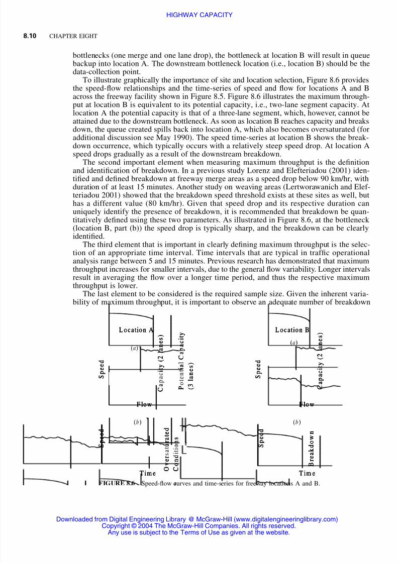
FIGURE 8.6 Speed-ow curves and time-series for freeway locations A and B.

bottlenecks (one merge and one lane drop), the bottleneck at location B will result in queuebackup into location A. The downstream bottleneck location (i.e., location B) should be thedata-collection point.

To illustrate graphically the importance of site and location selection, Figure 8.6 providesthe speed-ow relationships and the time-series of speed and ow for locations A and B

across the freeway facility shown in Figure 8.5. Figure 8.6 illustrates the maximum through-put at location B is equivalent to its potential capacity, i.e., two-lane segment capacity. Atlocation A the potential capacity is that of a three-lane segment, which, however, cannot beattained due to the downstream bottleneck. As soon as location B reaches capacity and breaksdown, the queue created spills back into location A, which also becomes oversaturated (foradditional discussion see May 1990). The speed time-series at location B shows the break-down occurrence, which typically occurs with a relatively steep speed drop. At location Aspeed drops gradually as a result of the downstream breakdown.

The second important element when measuring maximum throughput is the denitionand identication of breakdown. In a previous study Lorenz and Elefteriadou (2001) iden-tied and dened breakdown at freeway merge areas as a speed drop below 90 km/hr, withduration of at least 15 minutes. Another study on weaving areas (Lertworawanich and Elef-

teriadou 2001) showed that the breakdown speed threshold exists at these sites as well, buthas a different value (80 km/hr). Given that speed drop and its respective duration canuniquely identify the presence of breakdown, it is recommended that breakdown be quan-titatively dened using these two parameters. As illustrated in Figure 8.6, at the bottleneck (location B, part (b)) the speed drop is typically sharp, and the breakdown can be clearlyidentied.

The third element that is important in clearly dening maximum throughput is the selec-tion of an appropriate time interval. Time intervals that are typical in trafc operationalanalysis range between 5 and 15 minutes. Previous research has demonstrated that maximumthroughput increases for smaller intervals, due to the general ow variability. Longer intervalsresult in averaging the ow over a longer time period, and thus the respective maximumthroughput is lower.

The last element to be considered is the required sample size. Given the inherent varia-bility of maximum throughput, it is important to observe an adequate number of breakdown



HIGHWAY CAPACITY




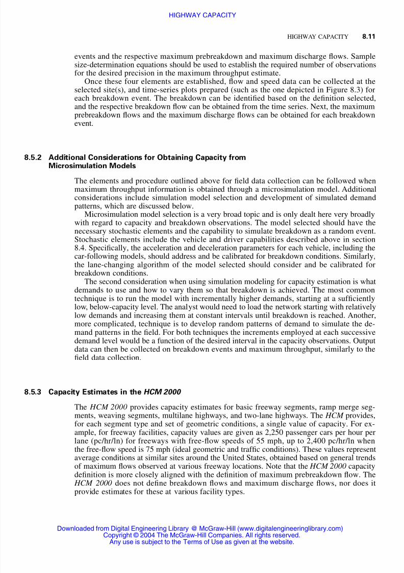
events and the respective maximum prebreakdown and maximum discharge ows. Samplesize-determination equations should be used to establish the required number of observationsfor the desired precision in the maximum throughput estimate.

Once these four elements are established, ow and speed data can be collected at theselected site(s), and time-series plots prepared (such as the one depicted in Figure 8.3) for

each breakdown event. The breakdown can be identied based on the denition selected,and the respective breakdown ow can be obtained from the time series. Next, the maximumprebreakdown ows and the maximum discharge ows can be obtained for each breakdownevent.

8.5.2 Additional Considerations for Obtaining Capacity fromMicrosimulation Models

The elements and procedure outlined above for eld data collection can be followed whenmaximum throughput information is obtained through a microsimulation model. Additional

considerations include simulation model selection and development of simulated demandpatterns, which are discussed below.Microsimulation model selection is a very broad topic and is only dealt here very broadly

with regard to capacity and breakdown observations. The model selected should have thenecessary stochastic elements and the capability to simulate breakdown as a random event.Stochastic elements include the vehicle and driver capabilities described above in section8.4. Specically, the acceleration and deceleration parameters for each vehicle, including thecar-following models, should address and be calibrated for breakdown conditions. Similarly,the lane-changing algorithm of the model selected should consider and be calibrated forbreakdown conditions.

The second consideration when using simulation modeling for capacity estimation is whatdemands to use and how to vary them so that breakdown is achieved. The most common

technique is to run the model with incrementally higher demands, starting at a sufcientlylow, below-capacity level. The analyst would need to load the network starting with relativelylow demands and increasing them at constant intervals until breakdown is reached. Another,more complicated, technique is to develop random patterns of demand to simulate the de-mand patterns in the eld. For both techniques the increments employed at each successivedemand level would be a function of the desired interval in the capacity observations. Outputdata can then be collected on breakdown events and maximum throughput, similarly to theeld data collection.

8.5.3 Capacity Estimates in the HCM 2000

The HCM 2000 provides capacity estimates for basic freeway segments, ramp merge seg-ments, weaving segments, multilane highways, and two-lane highways. The HCM provides,for each segment type and set of geometric conditions, a single value of capacity. For ex-ample, for freeway facilities, capacity values are given as 2,250 passenger cars per hour perlane (pc/hr/ln) for freeways with free-ow speeds of 55 mph, up to 2,400 pc/hr/ln whenthe free-ow speed is 75 mph (ideal geometric and trafc conditions). These values representaverage conditions at similar sites around the United States, obtained based on general trendsof maximum ows observed at various freeway locations. Note that the HCM 2000 capacitydenition is more closely aligned with the denition of maximum prebreakdown ow. The HCM 2000 does not dene breakdown ows and maximum discharge ows, nor does itprovide estimates for these at various facility types.



HIGHWAY CAPACITY



8.12 CHAPTER EIGHT

8.6 THE CAPACITY OF INTERRUPTED FLOW FACILITIES

Interrupted ow facilities are those where trafc ow experiences regular interruptions dueto trafc signs and signals. These include facilities such as signalized and unsignalizedintersections, and roundabouts, all of which are discussed in this section.

8.6.1 Signalized Intersections

The capacity of a signalized intersection depends very much on the phasing and timing plan.Trafc ow on a signalized intersection approach is regularly interrupted to serve conictingtrafc. Thus, the capacity of the approach is a function of the amount of green given to therespective movements within a given time interval. For example, if the cycle length at asignalized intersection is 90 seconds and the eastbound trafc is given 45 seconds of green,then the total amount of time that the approach is given the right-of-way within an hour is:

Total green time No. of cycles per hour Green time

3600/90 45 1800 sec

This corresponds to 1800/3600 50 percent of the full hour.In addition to this time restriction of right-of-way-availability, the time headways observed

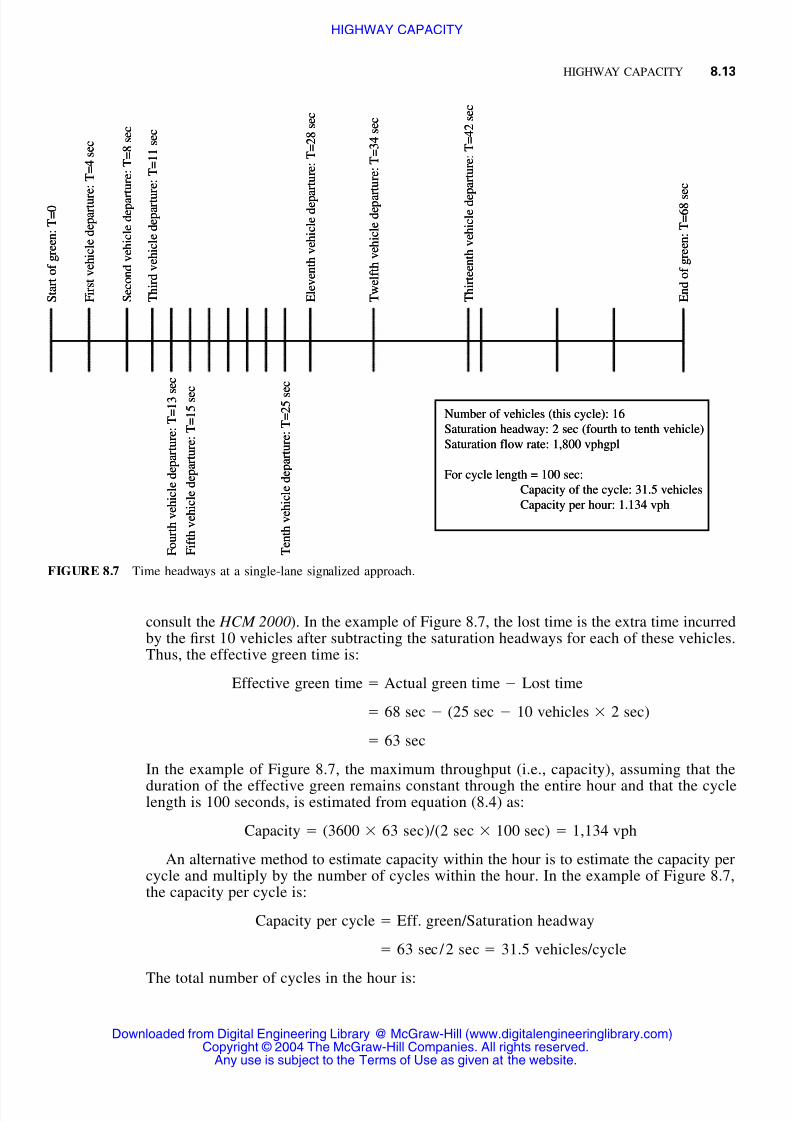
at the stop-line of a signalized intersection approach follow a different pattern as the trafcsignal changes from green to yellow to red and then back to green. Figure 8.7 illustrates aseries of consecutive time headways (also called discharge headways when referring toqueued vehicles at signalized intersection approaches) observed as vehicles depart from asingle-lane approach. The horizontal axis in the gure represents time (in seconds), whilethe vertical dashed lines represent events (signal changes and vehicle departures). At thebeginning of the green there were 10 vehicles queued at the approach. The volume during

this green interval is 16 vehicles. As shown, the rst discharge headway, measured from thebeginning of the green to the departure of the rst vehicle in the queue, is also the largestamong these rst 10 queued vehicles. Subsequent discharge headways gradually decreaseuntil they reach the ‘‘saturation headway’’ ( sh ) level for the approach, which is the minimumtime headway observed under conditions of continuous queuing—in this example 2 seconds.Next, saturation ow can be dened as the maximum throughput for the signalized inter-section approach, if the approach were given the green for a full hour. The saturation owfor a single lane can be calculated as:

Saturation flow (vehicles per hour of green) 3600/Average ( s )h

3600/ 2 1800 vehicles per hour of green per lane (vphgpl) (8.3)

Considering that each approach does not have the green for the full hour, the maximumthroughput that can be achieved at a signalized intersection approach depends on the percentof time the approach is given the green. Mathematically:

Max. throughput per lane Percent eff. green Saturation flow

g / C 3600/ s (3600 g) / (s C ) (8.4)h h

where g is the duration of effective green for the approach and C is the cycle length for theintersection.

The effective green is dened here as the time the approach is effectively used by thismovement, or the actual green time minus the lost time experienced due to start-up and

acceleration of the rst few vehicles (for discussion of lost time and its precise denition,



HIGHWAY CAPACITY




E n

d o

f g r e e n :

T =

6 8 s e c

S t a r t o

f g r e e n :

T =

0

F i r s t v e h

i c l e d e p a r t u r e :

T =

4 s e c

S e c o n

d v e h

i c l e d e p a r

t u r e :

T =

8 s e c

T h i r d v e h


T =

1 1 s e c

F o u r t h v e h


T =

1 3 s e c

F i f t h v e h


T =

1 5 s e c

T e n

t h v e h


T =

2 5 s e c

E l e v e n

t h v e h


T =

2 8 s e c

Number of vehicles (this cycle): 16Saturation headway: 2 sec (fourth to tenth vehicle)Saturation flow rate: 1,800 vphgpl

For cycle length = 100 sec:Capacity of the cycle: 31.5 vehiclesCapacity per hour: 1.134 vph

T w e l f t h v e h


T =

3 4 s e c

T h i r t e e n

t h v e h


T =

4 2 s e c

E n

d o

f g r e e n :

T =

6 8 s e c

S t a r t o

f g r e e n :

T =

0

F i r s t v e h


T =

4 s e c

S e c o n

d v e h

i c l e d e p a r

t u r e :

T =

8 s e c

T h i r d v e h


T =

1 1 s e c

F o u r t h v e h


T =

1 3 s e c

F i f t h v e h


T =

1 5 s e c

T e n

t h v e h


T =

2 5 s e c

E l e v e n

t h v e h


T =

2 8 s e c

Number of vehicles (this cycle): 16Saturation headway: 2 sec (fourth to tenth vehicle)Saturation flow rate: 1,800 vphgpl

For cycle length = 100 sec:Capacity of the cycle: 31.5 vehiclesCapacity per hour: 1.134 vph

T w e l f t h v e h


T =

3 4 s e c

T h i r t e e n

t h v e h

i c l e d e p a r t u r e

T =

4 2 s e c

FIGURE 8.7 Time headways at a single-lane signalized approach.

consult the HCM 2000 ). In the example of Figure 8.7, the lost time is the extra time incurredby the rst 10 vehicles after subtracting the saturation headways for each of these vehicles.Thus, the effective green time is:

Effective green time Actual green time Lost time

68 sec (25 sec 10 vehicles 2 sec)

63 sec

In the example of Figure 8.7, the maximum throughput (i.e., capacity), assuming that theduration of the effective green remains constant through the entire hour and that the cyclelength is 100 seconds, is estimated from equation (8.4) as:

Capacity (3600 63 sec)/(2 sec 100 sec) 1,134 vph

An alternative method to estimate capacity within the hour is to estimate the capacity percycle and multiply by the number of cycles within the hour. In the example of Figure 8.7,the capacity per cycle is:

Capacity per cycle Eff. green/Saturation headway

63 sec/2 sec 31.5 vehicles/cycle

The total number of cycles in the hour is:



HIGHWAY CAPACITY



8.14 CHAPTER EIGHT

Number of cycles 3600/100 sec 36 cycles/hr

Thus, the capacity within an hour is:

Capacity Capacity per cycle Number of cycles

31.5 vehicles per cycle 36 cycles 1,134 vph

8.6.2 Two-Way Stop-Controlled (TWSC) Intersections and Roundabouts

The operation of TWSC intersections and roundabouts (yield-controlled) is different thanthat of signalized intersections in that drivers approaching a stop or yield sign use their own

judgment to proceed through the junction through conicting trafc movements. Each driverof a stop- or yield-controlled approach must evaluate the size of gaps in the conicting trafcstreams, and judge whether he/she can safely enter the intersection or roundabout. Thecapacity of a stop- or yield-controlled movement is a function of the following parameters:

• The availability of gaps in the main (noncontrolled) trafc stream. Note that gap is denedin the HCM 2000 as time headway; elsewhere in the literature, however, gap is dened asthe time elapsing between the crossing of the lead vehicle’s rear bumper and the crossingof the following vehicle’s front bumper. In other words, the HCM 2000 gap denition(which will be used in this chapter) includes the time corresponding to the crossing of each vehicle’s length. The availability of gaps is a function of the arrival distribution of the main trafc stream.

• The gap acceptance characteristics and behavior of the drivers in the minor movements.The same gap may be accepted by some drivers and rejected by others. Also, when adriver has been waiting for a long time, he or she may accept a shorter gap, having rejectedlonger ones. The parameter most often used in gap acceptance is the critical gap, denedas the minimum time headway between successive major street vehicles, in which a minor-street vehicle can make a maneuver.

• The follow-up time of the subject movement queued vehicles. The follow-up time is thetime headway between consecutive vehicles using the same gap under conditions of con-tinuous queuing, and it is a function of the perception/reaction time of each driver.

• The utilization of gaps in the main trafc stream by movements of higher priority, whichresults in reduced opportunities for lower-priority movements (this is not applicable forroundabouts because there is only one minor movement).

The example provided below is a simplied illustration of the capacity estimation processfor a stop- or yield-controlled movement. The capacity of the northbound (NB) minor

through movement of Figure 8.8 will be estimated based on eld measurements at the in-tersection. There is only one major trafc stream at the intersection (eastbound, EB) and oneminor street movement (NB).

The critical gap was measured to be 4 seconds. It is assumed that any gap larger than 4seconds will be accepted by every driver, while every gap smaller than 4 seconds will berejected by every driver. The follow-up time was measured to be 3 seconds. Thus, for twovehicles to use a gap, it should be at least:

4 sec (first vehicle) 3 sec (second vehicle) 7 sec

Conversely, the following equation can be used to estimate the maximum number of vehiclesthat can use a gap of size X :



HIGHWAY CAPACITY




Minor Traffic Stream (NB)

Major TrafficStream (EB)

Gap

STOP


Major TrafficStream (EB)

Gap


Major TrafficStrea

m

(EB)

Gap

STOP

FIGURE 8.8 Capacity estimation for the NB through movement.

TABLE 8.1 Capacity Estimation for a Stop-Controlled Movement

Gap size(sec)

Col (1)

Usable Gap?(Y or N)Col (2)

Vehicles in NB movement thatcan use the gap (veh)

Col (3)

5 Y 12 N 07 Y 2

10 Y 34 Y 12 N 0

12 Y 317 Y 5

7 Y 23 N 02 N 03 N 0

13 Y 416 Y 5

TOTAL 103 sec 9 usable gaps 26 vehicles

Number of vehicles 1 (Gap Size X Critical Gap)/ Follow-up time (8.5)

Table 8.1 summarizes the eld data and subsequent calculations for the intersection of Figure 8.8, and provides the capacity estimate. Column (1) of Table 8.1 provides the gapsmeasured in the eld. Column (2) indicates whether the gap is usable, i.e., whether it islarger than the critical gap. Column (3) uses equation (8.5) to provide the number of vehicles



HIGHWAY CAPACITY



8.16 CHAPTER EIGHT

that can use each of the usable gaps. The total number of vehicles that can travel throughthe NB approach is the sum provided at the bottom of the column (3) (26 vehicles over 103seconds), or (3600/103) 26 909 vph, which is the capacity of the movement.

The HCM 2000 methodology for estimating the capacity of TWSC intersections is basedon the principles outlined above, using mathematical expressions of gap distributions and

probability theory for establishing the use of gaps by higher-priority movements.

8.7 SUMMARY AND CLOSING REMARKS

This chapter provided an overview of the concept of highway capacity, discussed the factorsthat affect it, and provided guidance on obtaining and using eld values of capacity.

The denition of capacity within the HCM has evolved over time. Even in the earliestpublications related to highway capacity there is a general recognition that the ‘‘maximumthroughput’’ of a highway facility is random, and thus there has been an effort to includethe expected variability of maximum volumes in the capacity denition. Recently, several

studies have used eld data and have proven that there is variability in the maximum sus-tained ows observed, in the range of several hundred vphpl. The cause of this variabilitylies in the microscopic characteristics of trafc, i.e., the individual spacing, time headway,and speed of each vehicle in the trafc stream and their variability. This chapter also providedthe fundamental principles of capacity estimation for uninterrupted and interrupted owfacilities, and provided guidance on obtaining capacity estimates in the eld and using sim-ulation.

The discussion provided in this chapter is not exhaustive and is only intended to providethe fundamental principles of capacity estimation for various highway facilities. Detailedmethodologies for estimating highway capacity for various facilities are provided in the HCM 2000, as well as elsewhere in the literature.

8.8 REFERENCES

Agyemang-Duah, K., and F. L. Hall. ‘‘Some Issues Regarding the Numerical Value of Highway Ca-pacity,’’ Highway Capacity and Level of Service—International Symposium on Highway Capacity,Karlsruhe, July 1991, pp. 1–15.

Bureau of Public Roads. 1950. Highway Capacity Manual. U.S. Department of Commerce, Bureau of Public Roads, Washington, DC.

Elefteriadou, L., and P. Lertworawanich. 2002. ‘‘Dening, Measuring and Estimating Freeway Capacity.’’Submitted to the Transportation Research Board.

Elefteriadou, L., R. P. Roess, and W. R. McShane. 1995. ‘‘The Probabilistic Nature of Breakdown at

Freeway-Merge Junctions.’’ Transportation Research Record 1484, 80–89.Evans, J., L. Elefteriadou, and G. Natarajan. 2001. ‘‘Determination of the Probability of Breakdown on

a Freeway Based on Zonal Merging Probabilities.’’ Transportation Research B 35:237–54.Fitzpatrick, K., L. Elefteriadou, D. Harwood, R. Krammes, N. Irizzari, J. McFadden, K. Parma, and J.

Collins. 1999. Speed Prediction for Two-Lane Rural Highways. Final Report, FHWA-99-171, 172, 173and 174, June, www.tfhrc.gov/safety/ihsdm/pdfarea.htm.

Flannery, A., L. Elefteriadou, P. Koza, and J. McFadden. 1998. ‘‘Safety, Delay and Capacity of Single-Lane Roundabouts in the United States.’’ Transportation Research Record 1646, 63–70.

Highway Research Board. 1965. Highway Capacity Manual. Highway Research Board, Special Report87, National Academies of Science, National Research Council Publication 1328.

Lertworawanich, P., and L. Elefteriadou. 2001. ‘‘Capacity Estimations for Type B Weaving Areas UsingGap Acceptance.’’ Transportation Research Record 1776, 24–34.

———. 2003. ‘‘A Methodology for Estimating Capacity at Ramp Weaves Based on Gap Acceptance andLinear Optimization.’’ Transportation Research B 37(5):459–83.



HIGHWAY CAPACITY




Lorenz, M., and L. Elefteriadou. 2001. ‘‘Dening Highway Capacity as a Function of the BreakdownProbability.’’ Transportation Research Record 1776, 43–51.

May, A. D. 1990. Trafc Flow Fundamentals . Englewood Cliffs: Prentice-Hall.Minderhoud, M. M., H. Botma, and P. H. L. Bovy. ‘‘Assessment of Roadway Capacity Estimation

Methods,’’ Transportation Research Record 1572, National Academy Prem, 1997, pp. 59–67.

Persaud, B. N., and V. F. Hurdle. ‘‘Freeway Capacity: Denition and Measurement Issues,’’ HighwayCapacity and Level of Service—International Symposium on Highway Capacity, Karlsruhe, July 1991,pp. 289–308.

Transportation Research Board (TRB). 2000. Highway Capacity Manual. National Research Council,TRB, Washington DC.

Wemple, E. A., A. M. Morris, and A. D. May. ‘‘Freeway Capacity and Flow Relationships,’’ HighwayCapacity and Level of Service—International Symposium on Highway Capacity, Karlsruhe, July 1991,pp. 439–456.



HIGHWAY CAPACITY



Downloaded from Digital Engineering Library @ McGraw Hill (www digitalengineeringlibrary com)

HIGHWAY CAPACITY

8 Highway capacity.pdf

Documents

Transcript of 8 Highway capacity.pdf