7(6,6'2&725$/ 6SDWLDO'HSWK %DVHG0HWKRGVIRU … · 7(6,6'2&725$/ 6sdwldo'hswk...

TESIS DOCTORAL

Spatial Depth-Based Methods for Functional Data

Autor:

Carlo Sguera

Director/es:

Pedro Galeano, Rosa Lillo

DEPARTAMENTO DE ESTADÍSTICA

Getafe, Junio 2014

Universidad Carlos III de Madrid

PH.D. THESIS

Spatial Depth-Based Methods for Functional

Data

Author:

Carlo Sguera

Advisors:

Pedro Galeano, Rosa Lillo

DEPARTMENT OF STATISTICS

Madrid, June, 2014

This dissertation was written in the Department of Statistics at Universidad Carlos III de

Madrid under the supervision of the Professors Pedro Galeano and Rosa Lillo. The author

was a visiting scholar at the Department of Biostatistics of Columbia University under the su-

pervision of Professors Sara Lopez-Pintado and Jeff Goldsmith in the period April-July 2013.

The author was supported by a scholarship for master studies (UC3M) and was subsequently

hired as a teaching and research assistant (PIF). Besides, the author and the advisors had the

partial support of the following research projects: Spanish Ministry of Science and Innovation

grant ECO2011-25706 and by Spanish Ministry of Economy and Competition grant ECO2012-

38442.

To Ilaria, Nunzia e Rino

Agradecimientos

Dos cosas antes de empezar, bueno, tres, pero una ya se nota: primero, voy a escribir en

espanol, o mejor, en “itanol”; segundo, es la primera vez que escribo algo ası, y no se como me

va a salir; y tercero, soy de los que dejan estas cosas para el final: de hecho me acabo de servir

una cervecita para celebrarlo. Bueno, a por ellos

El primer “grazie” va a mi “sorellina” Ilaria. Te quiero mucho y a ver si te veo por Madrid

para la defensa, me gustarıa mucho. Nunzia y Rino, mi mama y mi papa, ya se que va ser

mas difıcil veros por aquı, pero bueno, ya lo celebraremos en Barletta, os quiero. Y ya que

menciono Barletta, mi ciudad, quiero mandar un abrazo a todos mis amigos de alla (uno mas

fuerte a Michele) y a mi familia alargada (primos, primas, tıos, tıas y a los abuelos que ya

no estan, que pero se hubieran alegrado un monton en un dıa como este). Uno kilometros

mas alla esta Andria, donde hice la secundaria: un beso a todas mis companeras de clase (sı,

eran casi todas chicas, ¡que suerte!). De Andria una mencion especial se la merecen Ornella

(siguiendo a ella a Roma descubrı casualmente que existıa una Facultad de Estadıstica), y claro,

Daniele e Marcello, que luego fueron mis companeros de piso en Roma, y ahora son mucho

mas. Ellos me vieron dar mis primeros pasos como estadıstico, juntos a Popolino, ya que

tuvimos la gran suerte de que fuera a vivir con nosotros este chico tan pequenito, que pero es

un grande: Popolı, “si nu grus!!!”. Un saludo tambien a todos mis companeros de universidad,

y sobre todo a dos, Marco e Simone: “cdddaaaaa”. Y ya llegamos a Madrid, donde por cierto

hice tambien el Erasmus en la UC3M, y donde tuve la suerte de que me diera clases Juanmi,

quizas el profesor que me hizo pensar que volver a la UC3M para emprender este camino

podıa ser una buena idea, y de conocer a mucha gente, entre otros a Leo e Irmi: “pasta al

i

huevo, chicos”. Y ya llegamos a los ultimos seis anos en Madrid donde he tenido la suerte

de compartir momentos con gente como: Raqui, perdon si el primer dıa no te quise dejar el

abrigo, pero por suerte luego compartimos muchas cosas mas, porque compartir es vivirun

abrazo tambien a tu hermano Albe y a toda tu familia que me “adopto” un poco. Fresa, mi

compi de despacho, pero tambien de “notti magiche”. Juancho, otro que de “notti magiche”

entiende mucho. Mahomud, mi habibi, un amigo que te da todo. Otro habibi, Azad, que

cuando se fue le seguıa viendo por todas partes. Mariano, el de Roma. Demian, yo soy el

dıa y el la noche, pero al final nos lo estamos pasando bien. Audra, que se enfada un poco

cuando la llamo . . . (ella sabe), pero es con carino. Y tambien Ana Laura, Diana, Joao, Gabi,

Davidy muchos mas. Y finalmente, no por ser pelotas, el ultimo gracias a Rosa y a Pedro, que

es tambien gracias a ellos si he podido escribir estos agradecimientos. Ciao, Carlo.

ii

Abstract

In this thesis we deal with functional data, and in particular with the notion of functional

depth. A functional depth is a measure that allows to order and rank the curves in a functional

sample from the most to the least central curve. In functional data analysis (FDA), unlike in

univariate statistics where R provides a natural order criterion for observations, the ways how

several existing functional depths rank curves differ among them. Moreover, there is no agree-

ment about the existence of a best available functional depth. For these reasons among others,

there is still ongoing research in the functional depth topic and this thesis intends to enhance

the progress in this field of FDA.

As first contribution, we enlarge the number of available functional depths by introducing

the kernelized functional spatial depth (KFSD). In the course of the dissertation, we show that

KFSD is the result of a modification of an existing functional depth known as functional spa-

tial depth (FSD). FSD falls into the category of global functional depths, which means that the

FSD value of a given curve relative to a functional sample depends equally on the rest of the

curves in the sample. However, first in the multivariate framework, where also the notion of

depth is used, and then in FDA, several authors suggested that a local approach to the depth

problem may result useful. Therefore, some local depths for which the depth value of a given

observation depends more on close than distant observations have been proposed in the lit-

erature. Unlike FSD, KFSD falls in the category of local depths, and it can be interpreted as a

local version of FSD. As the name of KFSD suggests, we achieve the transition from global to

local proposing a kernel-type modification of FSD.

KFSD, as well as any functional depth, may result useful for several purposes. For in-

v

stance, using KFSD it is possible to identify the most central curve in a functional sample, that

is, the KFSD-based sample median. Also, using the p% most central curves, we can draw a

p%-central region (0 < p < 100). Another application is the computation of robust means such

as the α-trimmed mean, 0 < α < 1, which consists in the functional mean calculated after

deleting the proportion α of least central curves. The use of functional depths in FDA has gone

beyond the previous examples and nowadays functional depths are also used to solve other

types of problems. In particular, in this thesis we consider supervised functional classification

and functional outlier detection, and we study and propose methods based on KFSD.

Our approach to both classification and outlier detection has a main feature: we are inter-

ested in scenarios where the solution of the problem is not extremely graphically clear. In more

detail, in classification we focus on cases in which the different groups of curves are hardly rec-

ognizable looking at a graph, and we overlook problems where the classes of curves are easily

graphically detectable. Similarly, we do not deal with outliers that are excessively distant from

the rest of the curves, but we consider low magnitude, shape and partial outliers, which are

harder to detect. We deal with this type of problems because in these challenging scenarios it

is possible to appreciate important differences among both depths and methods, while these

differences tend to be much smaller in easier problems.

Regarding classification, methods based on functional depths are already available. In this

thesis we consider three existing depth-based procedures. For the first time, several functional

depths (KFSD and six more depths) are employed to implement these depth-based techniques.

The main result is that KFSD stands out among its competitors. Indeed, KFSD, when used

together with one of the depth based methods, i.e., the within maximum depth procedure,

shows the most stable and best performances along a simulation study that considers six dif-

ferent curve generating processes and for the classification of two real datasets. Therefore, the

results supports the introduction of KFSD as a new functional depth.

For what concerns outlier detection, we also consider some existing depth-based proce-

dures and the above-mentioned battery of functional depths. In addition, we propose three

new methods exclusively designed for KFSD. They are all based on a desirable feature for a

vi

functional depth, that is, a functional depth should assign a low depth value to an outlier. Dur-

ing our research, we have observed that KFSD is endowed with this feature. Moreover, thanks

to its local approach, KFSD in general succeeds in ranking correctly outliers that do not stand

out evidently in a graph. However, a low KFSD value is not enough to detect outliers, and it is

necessary to have at disposal a threshold value for KFSD to distinguish between normal curves

and outliers. Indeed, the three methods that we present provide alternative ways to choose a

threshold for KFSD. The simulation study that we carry out for outlier detection is similarly

extensive as in classification. Besides our proposals, we consider three existing depth-based

methods and seven depths, and two techniques that do not use functional depths. The results

of this second simulation study are also encouraging: the proposed KFSD-based methods are

the only procedures that have good correct outlier detection performances in all the six scenar-

ios and for the two contamination probabilities that we consider.

To summarize, in this thesis we will present a new local functional depth, KFSD, which will

turn out to be a useful tool in supervised classification, when it used in conjunction with some

existing depth-based methods, and in outlier detection, by means of some new procedures that

we will also present in this work.

vii

Resumen

El tema de esta tesis es el analisis de datos funcionales, y en particular de la nocion de pro-

fundidad funcional. Una medida de profundidad funcional permite ordenar las curvas de

una muestra funcional de la mas central a la menos central. Al contrario de lo que ocurre en

R donde existe una forma natural de ordenar las observaciones, en el analisis de datos fun-

cionales (FDA) no existe una forma unica de ordenar las curvas, y por tanto las diferentes pro-

fundidades funcionales existentes ordenan las curvas de distintas formas. Ademas, no existe

un acuerdo sobre la existencia de una profundidad funcional mejor para todas las situaciones

entre las disponibles. Por estas razones, entre otras, el tema de la nocion de profundidad fun-

cional es todavıa un area de estudio de investigacion activa, y esta tesis se propone colaborar

en los avances en este campo de FDA.

Como primera contribucion, en esta tesis se amplıa el numero de profundidades fun-

cionales disponibles mediante la introduccion de la profundidad espacial funcional kernel-

izada (KFSD). A lo largo de este trabajo, se muestra que KFSD es el resultado de una modifi-

cacion de una profundidad funcional existente conocida como profundidad espacial funcional

(FSD). FSD se puede englobar dentro de la categorıa de las profundidades funcionales glob-

ales, lo que significa que el valor de FSD para una curva dada, en relacion con una muestra

funcional, depende igualmente del resto de las curvas en la muestra. Sin embargo, como en el

contexto multivariante, donde tambien se utiliza el concepto de profundidad, varios autores

han sugerido que un enfoque local para la definicion de una profundidad puede resultar util

tambien en FDA. Por este motivo, en la literatura se han propuesto algunas profundidades

locales para las que el valor de la profundidad de una observacion depende mas de las ob-

ix

servaciones cercanas que de las distantes. A diferencia de FSD, KFSD se puede clasificar en

la categorıa de las profundidades locales, y puede ser interpretada como una version local de

FSD. Como el nombre de KFSD sugiere, la transicion de lo global a lo local se lograra mediante

una modificacion de FSD basada en el uso de los kernels.

KFSD, ası como cualquier otra profundidad funcional, puede resultar util para varios

propositos en el ambito del analisis estadıstico de datos. Por ejemplo, usando KFSD es posible

identificar la curva mas central en una muestra funcional, es decir, la mediana de la muestra

segun KFSD. Ademas, utilizando el p% de las curvas centrales, es posible definir la p%-region

central (0 < p% < 100). Otra aplicacion es el calculo de medias robustas, como por ejemplo la

α-media truncada, con 0 < α < 1, que consiste en la media funcional calculada sin considerar

la proporcion α de las curvas menos centrales. El uso de las profundidades funcionales en FDA

ha ido mas alla de los ejemplos anteriores, y en la actualidad las profundidades funcionales

tambien se utilizan para resolver otros tipos de problemas. En particular, en esta tesis se con-

sideran la clasificacion supervisada funcional y la deteccion de curvas atıpicas, y se estudian y

proponen metodos basados en KFSD.

El enfoque que se presenta en esta tesis en clasificacion y deteccion de atıpicos tiene una

caracterıstica principal: el foco del trabajo esta puesto en escenarios en los que la solucion del

problema no resulta muy clara graficamente. Especıficamente, en el apartado de clasificacion

se consideran casos en los que los diferentes grupos de curvas son apenas reconocibles mi-

rando un grafico, mientras que no se consideran problemas donde las clases de las curvas son

facilmente detectables graficamente. De manera similar, no esta entre nuestros objetivos de-

tectar curvas atıpicas que estan excesivamente alejadas graficamente del resto de las curvas, y

por el contrario se consideran atıpicos de baja magnitud, de forma y atıpicos parciales, que son

mas difıciles de detectar con los procedimientos que ya existen en la literatura. En este sentido,

se pondra en evidencia que en este tipo de problemas existen diferencias sustanciales entre las

profundidades y los metodos de analisis, mientras que estas diferencias tienden a ser menores

en problemas mas sencillos o visualmente mas evidentes.

En relacion con el problema de clasificacion funcional, existen en la literatura metodos basa-

x

dos en el uso de las profundidades funcionales. En esta tesis se consideran tres procedimien-

tos de este tipo, y por primera vez se combinan con varias profundidades funcionales (KFSD

y seis mas) con el objetivo de establecer comparativas entre metodos y/o profundidades con

los mismos escenarios. El resultado principal que se observa es que KFSD se destaca entre

sus competidores. De hecho, KFSD, cuando se utiliza junto a uno de los metodos conocido

como el procedimiento de profundidad maxima en los grupos, muestra los resultados mejores

y mas estables a lo largo de un estudio de simulacion que considera seis procesos diferentes

para generar las curvas, ası como en la clasificacion de dos conjuntos de datos reales. Por lo

tanto, los resultados obtenidos sustentan la introduccion de KFSD como nueva profundidad

funcional.

Por lo que se refiere a la deteccion de curvas atıpicas, tambien se consideran algunos pro-

cedimientos ya existentes basados en el uso de la nocion de profundidad y el grupo de sietes

profundidades mencionado arriba. Ademas, se proponen tres nuevos metodos disenados ex-

clusivamente para KFSD. Todos ellos se basan en una caracterıstica deseable en una profun-

didad funcional, es decir, que esta asigne un valor de profundidad baja a una curva atıpica.

Durante nuestra investigacion, se ha observado que KFSD posee esta caracterıstica. Ademas,

gracias a su enfoque local, KFSD es en general capaz de ordenar correctamente los atıpicos

que no se destacan claramente en un grafico. Sin embargo, un valor bajo de KFSD no es su-

ficiente para detectar curvas atıpicas, y es necesario tener a disposicion un valor umbral para

KFSD para distinguir entre curvas normales y atıpicas. De hecho, los tres metodos que se

presentan ofrecen formas alternativas para elegir un umbral para KFSD. Desde un punto de

vista metodologico, estos procedimientos estan respaldados por resultados teoricos de corte

probabilısticos. El estudio de simulacion que se lleva a cabo para la deteccion de atıpicos es

igualmente extenso como en el caso de clasificacion. Ademas de nuestras propuestas, se con-

sideran tres metodos existentes que estan basados en el uso de profundidades funcionales y

dos tecnicas que no utilizan profundidades funcionales. Los resultados de este segundo estu-

dio de simulacion son tambien positivos: los metodos basados en KFSD que se proponen en

esta tesis resultan ser los procedimientos que detectan mejor los atıpicos para un conjunto de

xi

seis escenarios simulados y para las dos probabilidades de contaminacion que se consideran.

En resumen, en esta tesis se presenta una nueva profundidad funcional local, KFSD, que

resulta ser una herramienta util en clasificacion supervisada cuando se utiliza conjuntamente

con algunos metodos basados en el uso de profundidades, y en la deteccion de curvas atıpicas

por medio de algunos nuevos procedimientos que tambien se presentan en este trabajo.

xii

Contents

List of Figures xix

List of Tables xxi

1 Introduction 1

1.1 The Notion of Functional Depth . . . . . . . . . . . . . . . . . . . . . . . . . . . . . 4

1.2 Depth-based Functional Methods . . . . . . . . . . . . . . . . . . . . . . . . . . . . 8

1.3 Structure of the Thesis . . . . . . . . . . . . . . . . . . . . . . . . . . . . . . . . . . 11

2 The Kernelized Functional Spatial Depth 15

2.1 Introduction . . . . . . . . . . . . . . . . . . . . . . . . . . . . . . . . . . . . . . . . 15

2.2 Other Functional Depths . . . . . . . . . . . . . . . . . . . . . . . . . . . . . . . . . 16

2.3 The Functional Spatial Depth and Associated Quantiles . . . . . . . . . . . . . . . 18

2.4 The Kernelized Functional Spatial Depth . . . . . . . . . . . . . . . . . . . . . . . 20

2.5 From Global to Local Depths . . . . . . . . . . . . . . . . . . . . . . . . . . . . . . 23

2.6 Conclusions . . . . . . . . . . . . . . . . . . . . . . . . . . . . . . . . . . . . . . . . 29

3 Supervised Functional Classification 31

3.1 Introduction . . . . . . . . . . . . . . . . . . . . . . . . . . . . . . . . . . . . . . . . 31

3.2 The Supervised Functional Classification Problem . . . . . . . . . . . . . . . . . . 32

3.3 Simulation Study . . . . . . . . . . . . . . . . . . . . . . . . . . . . . . . . . . . . . 34

3.4 Real Data Study . . . . . . . . . . . . . . . . . . . . . . . . . . . . . . . . . . . . . . 45

xv

3.4.1 Growth Data . . . . . . . . . . . . . . . . . . . . . . . . . . . . . . . . . . . 45

3.4.2 Phoneme Data . . . . . . . . . . . . . . . . . . . . . . . . . . . . . . . . . . 49

3.5 Conclusions . . . . . . . . . . . . . . . . . . . . . . . . . . . . . . . . . . . . . . . . 52

4 Functional Outlier Detection 55

4.1 Introduction . . . . . . . . . . . . . . . . . . . . . . . . . . . . . . . . . . . . . . . . 55

4.2 Outlier Detection for Functional Data . . . . . . . . . . . . . . . . . . . . . . . . . 57

4.3 Simulation Study . . . . . . . . . . . . . . . . . . . . . . . . . . . . . . . . . . . . . 62

4.4 Real Data Study: Nitrogen Oxides (NOx) Data . . . . . . . . . . . . . . . . . . . . 72

4.5 Conclusions . . . . . . . . . . . . . . . . . . . . . . . . . . . . . . . . . . . . . . . . 75

4.6 Appendix . . . . . . . . . . . . . . . . . . . . . . . . . . . . . . . . . . . . . . . . . 76

5 Conclusions 81

5.1 Research Lines . . . . . . . . . . . . . . . . . . . . . . . . . . . . . . . . . . . . . . . 83

References 87

xvi

List of Figures

1.1 Three real functional datasets . . . . . . . . . . . . . . . . . . . . . . . . . . . . . . 3

2.1 Showing the differences between global and local depths . . . . . . . . . . . . . . 24

2.2 Examples of contaminated datasets: clear contamination (top) and faint contam-

ination (bottom). The solid curves are normal curves and the dashed curves are

outliers . . . . . . . . . . . . . . . . . . . . . . . . . . . . . . . . . . . . . . . . . . . 26

2.3 Comparison of depth-based rankings . . . . . . . . . . . . . . . . . . . . . . . . . 27

2.4 Comparison of KFSD-based rankings . . . . . . . . . . . . . . . . . . . . . . . . . 28

3.1 Simulated datasets from CGP1, CGP2, CGP1out and CGP2out . . . . . . . . . . . . 37

3.2 Simulated datasets from CGP3 and CGP4 . . . . . . . . . . . . . . . . . . . . . . . 43

3.3 Growth curves . . . . . . . . . . . . . . . . . . . . . . . . . . . . . . . . . . . . . . . 46

3.4 Growth curves: highlighting some interesting curves for the classification problem 48

3.5 Phoneme curves . . . . . . . . . . . . . . . . . . . . . . . . . . . . . . . . . . . . . . 50

4.1 Simulated datasets from MM1, MM2, MM3, MM4, MM5 and MM6 . . . . . . . . 64

4.2 Example of a training sample of peripheral curves . . . . . . . . . . . . . . . . . . 66

4.3 Boxplots of the selected bandwidths for KFSD . . . . . . . . . . . . . . . . . . . . 71

4.4 NOx curves . . . . . . . . . . . . . . . . . . . . . . . . . . . . . . . . . . . . . . . . 73

4.5 NOx curves: highlighting some detected outliers . . . . . . . . . . . . . . . . . . . 74

xix

List of Tables

2.1 Percentages of times a depth assigns a value among the nout,j lowest ones to an

outlier. Types of outliers: clear and faint . . . . . . . . . . . . . . . . . . . . . . . . 26

3.1 Supervised classification: CGP1 . . . . . . . . . . . . . . . . . . . . . . . . . . . . . 40


3.3 Supervised classification: CGP1out . . . . . . . . . . . . . . . . . . . . . . . . . . . 40

3.4 Supervised classification: CGP2out . . . . . . . . . . . . . . . . . . . . . . . . . . . 40

3.5 Cross-validation and best performing percentiles: CGP1, CGP2, CGP1out and

CGP2out . . . . . . . . . . . . . . . . . . . . . . . . . . . . . . . . . . . . . . . . . . 41



3.8 Cross-validation and best performing percentiles: CGP3 and CGP4 . . . . . . . . 44

3.9 Supervised classification: Growth data and T1 . . . . . . . . . . . . . . . . . . . . 46

3.10 Supervised classification: Growth data and T2 . . . . . . . . . . . . . . . . . . . . 47

3.11 Cross-validation and best performing percentiles: Growth data . . . . . . . . . . 47

3.12 Supervised classification: Phoneme data and T1 . . . . . . . . . . . . . . . . . . . 51

3.13 Supervised classification: Phoneme data and T2 . . . . . . . . . . . . . . . . . . . 51

3.14 Cross-validation and best performing percentiles: Phoneme data . . . . . . . . . 51

4.1 Outlier detection: MM1 . . . . . . . . . . . . . . . . . . . . . . . . . . . . . . . . . 67


xxi





4.7 Outlier detection: NOx data . . . . . . . . . . . . . . . . . . . . . . . . . . . . . . . 73

xxii

La poesia non e di chi la scrive,e di chi gli serve!(Mario Ruoppolo to Pablo Neruda in Il Postino)

Chapter 1

Introduction

The technological advances of the last decades in fields such as chemometrics, engineering,

finance, growth analysis or medicine among others have allowed to observe random samples

of curves. In these cases it is common to assume that the curves have been generated by a

stochastic function and to refer to them as functional data. More precisely, a functional datum

y is an observation of a functional random variable Y ∈ H, where H is an infinite-dimensional

(functional) space. Alternatively, Y can also be interpreted as a stochastic process Y (s), s ∈ I,

where I is an interval in R, and the functional datum expressed as y(s).

In practice, a functional datum y(s) is always observed at a finite number of evaluation

points, that is, in the form of y(s) = (y(s1), . . . , y(sm)), where s = (s1, . . . , sm) is the set of

domain points where y(s) has been measured. However, even if y(s) is a vector, there are at

least three reasons why it is harmful to treat functional data as multivariate data.

1. The sets of domain points where the functional data of a sample are measured may differ

in size and/or elements among them. Moreover, for each observation the order of the

vector s contains an important amount of information and permutations of its elements

are not allowed, unlike in the multivariate case.

2. Any curve is a realization of a stochastic function with a certain dependence structure.

Consequently, functional data are often autocorrelated. Therefore, it is hard to analyze

1

INTRODUCTION 2

functional data by means of standard multivariate procedures because they usually fail

in presence of autocorrelation.

3. Functional samples may contain less curves than evaluation points or, in multivariate

jargon, less rows than columns. It is well known that matrices with more columns than

rows are hardly handled by multivariate techniques.

As a response to the difficulty described above of multivariate data analysis to deal with

functional data, the area of statistics known as functional data analysis (FDA) has arisen in

recent years. Two seminal and complementary books about FDA, one parametric and the other

nonparametric, are Ramsay and Silverman (2005) and Ferraty and Vieu (2006), respectively.

More recently, Horvath and Kokoszka (2012) focused on inference and asymptotic theory for

functional data, whereas Cuevas (2014) presented a partial overview of the state of art in FDA

theory. To give an idea of the kind of data FDA deals with, we show in Figure 1.1 three real

datasets that are considered in this thesis. They are:

• growth curves of 54 heights of girls measured at a common discretized set of 31

nonequidistant ages between 1 and 18 years (Ramsay and Silverman 2005);

• 100 log-periodograms of length 150 corresponding to recordings of speakers pronounc-

ing the phoneme “aa” (Ferraty and Vieu 2006);

• 76 nitrogen oxides (NOx) emission level daily curves measured every hour close to an in-

dustrial are in Poblenou (Barcelona). All the curves correspond to working days (Febrero

et al. 2008).

Before closing this introduction, we make a brief remark on a FDA aspect that is not central

in this thesis, but it is worth to mention. According to Cuevas (2014), a functional datum y(s)

may require a preliminary treatment to either reduce its dimension or remove noise. Among

other alternatives, both objectives can be achieved through basis representation: let ej(s) be

a basis system of H, then y(s) can be substituted by a truncated basis representation given by

INTRODUCTION 3

5 10 15

8010

012

014

016

018

0

Growth

0 50 100 150

05

1015

2025

Phoneme

0 5 10 15 20

010

020

030

040

0

NOx

Figure 1.1: Three real functional datasets: growth curves of girls (top left), log-periodograms of the phoneme “aa” (top right), daily curves of NOx levels (bottom)

y(s) =

J∑j=1

cjej(s),

where J denotes the number of basis functions to use and cj the coefficients to be chosen

according to some criteria, e.g., least squares

m∑k=1

y(sk)−J∑j=1

cjej(sk)

2

.

Clearly, the choices of ej(s), J and the criterion to select cj are very important aspects, but

we do not discuss them in the thesis since they are beyond our scope. For more details on this

FDA issue, we recommend the book by Ramsay and Silverman (2005).

INTRODUCTION 4

1.1 The Notion of Functional Depth

In the previous section we discussed the juxtaposition of multivariate and functional data anal-

ysis. However, their differences did not prevent multivariate techniques to inspire advances

in FDA. A good example of the collaboration between the two areas is given by the extension

of the notion of data depth from the multivariate to the functional framework.

The idea of data depth was born in the multivariate context in a successful attempt to ex-

tend the univariate notion of order statistics to multidimensional spaces. Univariate order

statistics allow to rank data from the smallest to the largest observation and to evaluate the

degree of centrality of a point relative to a probability distribution or a sample. Moving to Rd,

d ≥ 2, although Rd lacks the natural order of R, it is still interesting to have a center-outward

ordering criterion and the notion of multivariate depth succeeds in providing it. According to

Serfling (2006), a multivariate depth is a function that measures how deep (or central) a point

x ∈ Rd is relative to the probability distribution P . To give an idea of how a multivariate depth

should work, consider a P with a unique mode Mo anda certain tail. Then, the depth value of

x should be high for x = Mo and low for x equal to a value in the tail region.

Several implementations of the notion of multivariate depth have been proposed in the

literature. For an overview on this topic, see for example Liu et al. (1999) or Zuo and Ser-

fling (2000). Next, we report the definitions of three multivariate depths. First, the halfspace

depth (Tukey 1975), which is defined as the minimum probability mass carried by any closed

halfspace H ∈ Rd containing x. More precisely,

Definition 1.1. Halfspace (or Tukey) depth (Tukey 1975)

The halfspace depth of x ∈ Rd relative to P on Rd is given by

HSD(x, P ) = infHPr(H) : x ∈ H . (1.1)

Second, the simplicial depth (Liu 1990), which is defined as the probability that x belongs

to a random simplex S ∈ Rd, that is,

INTRODUCTION 5

Definition 1.2. Simplicial depth (Liu 1990)

The simplicial depth of x ∈ Rd relative to P on Rd is given by

SID(x, P ) = Pr (x ∈ S (y1, . . . ,yd+1)) , (1.2)

where S (y1, . . . ,yd+1) denotes the d-dimensional simplex with vertices y1, . . . ,yd+1.

Third, the spatial depth (Serfling 2002), that uses the geometry of multivariate data clouds

and is connected with a notion of multivariate quantiles as we show later.

Definition 1.3. Spatial depth (Serfling 2002)

Let Y be a random variable having probability distribution P on Rd and F be the associated

cumulative distribution of Y. The spatial depth of x ∈ Rd relative to P is given by

SD(x, P ) = 1−∥∥∥∥∫ S(x− y)dF (y)

∥∥∥∥E

= 1− ‖E [S(x−Y)]‖E , (1.3)

where ‖·‖E is the Euclidean norm in Rd and S : Rd → Rd is the spatial sign function given by

S(x) =

x‖x‖E , x 6= 0,

0, x = 0.

Among the previous three multivariate depths, SD has certainly the most important role

for the development of this thesis. For this reason, we report two features of the multivariate

spatial depth. First, as mentioned above, SD is connected with the notion of multivariate

spatial quantile introduced by Chaudhuri (1996):

Definition 1.4. Spatial quantile (Chaudhuri 1996)

Let Y be a random variable having probability distribution P on Rd. Consider u ∈ Rd such

that ‖u‖E < 1. Then, QP (u) is the uth spatial quantile of Y if and only if QP (u) is the value of

q which minimizes

E [Ψ(u,Y − q)−Ψ(u,Y)] ,

INTRODUCTION 6

where, for y ∈ Rd, Ψ(u,y) = ‖y‖E + 〈u,y〉E , and 〈u,y〉E is the Euclidean inner product of u

and y.

Then, it can be shown that under some mild conditions QP (u) and SD(x, P ) are linked in

the following way:

‖Q−1P (x)‖E = 1− SD(x, P ). (1.4)

Therefore, if x has a high spatial depth value, its associated spatial quantile u has a low norm,

and vice versa.

Second, SD(x, P ) depends on the whole P , that is, SD as well as HSD and SID tackle the

depth problem through an approach that we describe as “global”. However, in some analy-

ses it may be recommended to focus on narrower neighborhoods of P and tackle the depth

problem with a “local approach”. With the aim of showing how a local approach can be im-

plemented, we next briefly describe the local versions of the global depths HSD, SID and SD

that have been proposed in the literature:

• the local halfspace depth LHSD (Agostinelli and Romanazzi 2011), which replaces closed

halfspaces with closed slabs. Denote with Hu(a) the closed halfspace z ∈ Rd : u′z ≥

a, u′u = 1. Then, (1.1) can be written as

HSD(x, P ) = infu:u′u=1

Pr(Hu(u′x)). (1.5)

A closed slab SLu(a, a+ τ) between two parallel closed halfspaces Hu(a) and Hu(a+ τ)

is the intersection between the positive side of Hu(a) and the negative side of Hu(a+ τ).

Then, LHSD is given by the following modification of (1.5):

LHSD(x, P, τ) = infu:u′u=1

Pr(SLu(u′x, u′x+ τ)).

• the local simplicial depth LSID (Agostinelli and Romanazzi 2011), which only considers

INTRODUCTION 7

simplices with size no greater than a fixed threshold τ and is given by the following

modification of (1.2):

LSID(x, P, τ) = Pr (x ∈ S (y1, . . . ,yd+1) : v(S (y1, . . . ,yd+1)) ≤ τ) ,

where v(S (y1, . . . ,yd+1)) denotes the volume of the simplex with vertices y1, . . . ,yd+1.

• the kernelized spatial depth KSD (Chen et al. 2009), which is basically based on consid-

ering S(x− y) in (1.3) through a kernel function that reduces the effect of y on the depth

of x for y distant from x.

The notion of multivariate depth has been extended to functional data. In FDA, a depth

has a similar purpose, that is, it allows to obtain a center-outward ordering criterion for curves,

and different implementations already exist in the FDA literature. For example, Chakraborty

and Chaudhuri (2014) defined the functional version of SD(x, P ), the functional spatial depth

function FSD(x, P ), where now x is an element of an infinite-dimensional Hilbert space H

and P is a probability distribution on H. As well as SD, FSD is a global-oriented depth. We

give its formal definition in Chapter 2, where we also present the functional extension of the

notion of spatial quantile function, FQP (u), where now u ∈ H such that ‖u‖ < 1, and ‖ · ‖ is

the norm derived from the inner product 〈·, ·〉 in H (Chaudhuri 1996). In the same chapter we

show that the relationship given by (1.4) extends to the functional framework, and therefore

also FSD(x, P ) and FQP (u) are linked.

The main contribution of this thesis is the definition of a new functional depth. Indeed, we

define the kernelized functional spatial depth (KFSD) which can be interpreted in two ways:

first, KFSD is a functional extension of the multivariate KSD proposed by Chen et al. (2009);

second, KFSD is a local-oriented version of the global-oriented FSD. Then, we use KFSD to

solve functional statistical problems that may require an analysis at a local level. We mainly

focus on supervised classification and outlier detection and we show that KFSD represents a

useful tool to solve such problems.

Along the thesis, besides FSD and KFSD, we consider other functional depths that we next

INTRODUCTION 8

briefly introduce: Fraiman and Muniz (2001) defined the Fraiman and Muniz depth (FMD),

which tries to measure how long a curve remains in the middle of a sample. Cuevas et al.

(2006) proposed the h-modal depth (HMD), which tries to measure how densely a curve is sur-

rounded by other curves. Cuesta-Albertos and Nieto-Reyes (2008) and Cuevas and Fraiman

(2009) proposed the random Tukey depth (RTD) and the integrated dual depth (IDD), respec-

tively. Both depths are based on the computation of K random one-dimensional projections

of the curves, but they differ on how the projections are treated: RTD is given by the mini-

mum of the univariate Tukey depth values of the projections, IDD is given by the average of

the univariate simplicial depth values of the projections. Finally, Lopez-Pintado and Romo

(2009) proposed the band and modified band depths. In particular, the modified band depth

(MBD) is based on all the possible bands defined by the graphs on the plane of 2, 3, . . . and J

curves, and on a measure of the sets where another curve is inside these bands. We provide

the definitions of these functional depths in Chapter 2.

1.2 Depth-based Functional Methods

In what follows we often use the notion of i. i. d. functional sample that may refer alternatively

to:

1. an i. i. d. random sample of size n generated from the random variable Y ∈ H. In this

case we use the notation Yn = y1, . . . , yn;

2. an i. i. d. random sample of size n generated from the stochastic process Y (s), s ∈ I. In

this case we use the notation Yn(s) = y1(s), . . . , yn(s);

3. an i. i. d. random sample of size n generated from the stochastic process Y (s), s ∈ I

whose ith component has been observed at si = (s1i , . . . , smi), i ∈ 1, . . . , n. In this case

we use the notation Yn(s) = y1(s1), . . . , yn(sn).1

1if si 6= sj for some i, j ∈ 1, . . . , n, it may be necessary a preliminary step to estimate the curves at a commonset of domain points. In this thesis, when the data require such preliminary treatment, we carry out the estimationusing cubic spline interpolation. Other techniques can be used for this task.

INTRODUCTION 9

A functional sample (e.g., Yn) can be analyzed using a functional depth. For example,

functional location estimation of the center of Y can be provided by either non-depth-based or

depth-based statistics. A natural estimation of the center of Y is given by the functional mean,

µ =1

n

n∑i=1

yi.

Clearly, the computation of µ does not require the use of a functional depth. However, a depth

analysis of Yn provides a center-outward ordering of the observations, i.e., Y(n) = y(1), . . . ,

y(n), where y(1) and y(n) are the curves in Yn with minimum and maximum depth, respec-

tively. Y(n) provides an alternative to µ, that is, the functional depth-based median given by

the deepest/most central observation in Yn, Me = y(n). Another substitute for µ may be the

functional depth-based α-trimmed mean µα, 0 < α < 1, that can be obtained as follows: com-

pute rα = αn and take the smallest integer greater or equal than rα, drαe. Then,

µα =1

n

n∑i=drαe

y(i).

Moreover, the information contained in Y(n) allows to estimate locations other than the

center of Y by means of the notion of functional depth-based percentiles: let 0% ≤ p ≤ 100%,

rp = pn100 and rp be the nearest integer to rp, then the p depth-based percentile of Yn is given by

y(rp).

Besides for location estimation, functional depths can be used to build methods that are

robust to functional outliers, i.e., curves generated by a different random variable than the one

of the normal curves. For instance, supervised functional classification is one of the problems

that has been tackled using the notion of depth. In a supervised functional classification prob-

lem there are some labeled training curves that belong to two or more groups and the goal is to

classify some test curves with unknown class membership. Lopez-Pintado and Romo (2006)

and Cuevas et al. (2007) proposed three depth-based classification methods which are espe-

cially devised to deal with functional samples where the presence of outlying curves cannot

be discarded. They are the distance to the trimmed mean method (DTM, Lopez-Pintado and

INTRODUCTION 10

Romo 2006), the weighted averaged distance method (WAD, Lopez-Pintado and Romo 2006)

and the within maximum depth method (WMD, Cuevas et al. 2007). We formally present them

in Chapter 3, but here we anticipate that the robustness to outliers of DTM, WAD and WMD

is achieved thanks to the use of a functional depth: in DTM, the decision rule depends on the

group depth-based trimmed means, that are resistant to outliers; in WAD, the classification is

done giving more weight to those curves that are deeper within the group training samples,

and outliers have usually low depth values; in WMD, the class of an unlabeled curve depends

on its depth values relative to the different training groups, and these values are barely affected

by outliers. We enhance the study of DTM, WAD and WMD by studying their performances

when they are used in conjunction with KFSD and the other above-mentioned existing func-

tional depths. In particular, we consider supervised functional classification problems where

the differences between groups are not extremely clear-cut or the data may contain outlying

curves, and we show that in these challenging scenarios a local approach based on the use of

KFSD leads to good results.

An alternative strategy to the construction of robust functional methods is outlier detec-

tion. When a sample of curves is ordered from the most to the least central curve using a

functional depth, if any outlier is in the sample, its depth is expected to be among the lowest

values. Therefore, it is reasonable to build outlier detection methods based on this feature.

Indeed, methods of this nature already exist in the literature. For example, Febrero et al. (2008)

proposed to label as outliers those curves with depth values lower than a certain threshold. As

functional depths, they considered three alternatives, i.e., the Fraiman and Muniz depth FMD

(Fraiman and Muniz 2001), the h-modal depth HMD (Cuevas et al. 2006) and the integrated

dual depth IDD (Cuevas and Fraiman 2009), and they proposed two bootstrap procedures

based on depth-based trimmed and weighted resampling to determine the depth threshold.

Also, Sun and Genton (2011) introduced the functional boxplot, which is constructed using the

ordering provided by the modified band depth MBD (Lopez-Pintado and Romo 2009). Then,

the functional boxplot allows to detect outliers as well as the standard boxplot does. Clearly,

the use of a functional depth is only one of the possible strategies for tackling the functional

INTRODUCTION 11

outlier detection problem. For example, Hyndman and Shang (2010) proposed to reduce the

outlier detection problem from functional to multivariate data by means of functional prin-

cipal component analysis (FPCA), and to use two alternative multivariate techniques on the

scores to detect outliers, i.e., the bagplot and the high density region boxplot. In this thesis,

we contribute to the FDA literature on outlier detection by enlarging the number of available

procedures. Indeed, we present three new methods that are based on smoothed resampling

techniques and allow to select a threshold for KFSD to detect outliers. Similarly as for clas-

sification, we evaluate these new procedures in challenging scenarios: we focus on low mag-

nitude, shape and partial outliers, that is, on outliers that are difficult to recognize, and we

observe results that support the proposed KFSD-based outlier detection methods.

1.3 Structure of the Thesis

This thesis contains five chapters. In the current chapter we discussed some FDA issues, we

presented three real functional datasets and we introduced the notion of functional depth. To

do that, we also recalled some global and local multivariate depths and described how the

concept of depth has been extended to FDA. Finally, we recalled some examples of how a

functional depth can help in doing statistics in FDA, e.g., location estimation, supervised clas-

sification and detection of outliers.

The contributions of this dissertation are developed in Chapters 2, 3 and 4. In Chapter 2

we present a new functional depth, the kernelized functional spatial depth (KFSD). KFSD is a

depth relying on an approach that is both spatial and local. Its local orientation is based on the

use of kernel methods that allow the depth value of a curve x to depend more on the curves

lying in a narrow neighborhood of x. By means of motivating examples, we show that the

local approach behind KFSD results useful to analyze functional samples having for instance

a structure that deviates from unimodality or that are contaminated by outliers. In Sections 2.3

and 2.2, we present the other existing functional depths that we use in this thesis (FMD, HMD,

RTD, IDD, MBD and FSD).

INTRODUCTION 12

In Chapter 3 we use KFSD to perform supervised classification. After describing the sta-

tistical problem of functional discrimination, we present three existing depth-based methods

(DTM, WAD and WMD) and carry out an extensive simulation study. The main feature of the

study, and a novelty in the field, is that we focus on scenarios where the difference between

groups are not extreme. We show that in these scenarios the use of KFSD together with some of

the depth-based classification methods leads to competitive results. In Section 3.4 we classify

the curves of two real datasets and we confirm the good results observed with the simulated

curves.

In Chapter 4 we deal with outlier detection. As for classification, the strategy consists in us-

ing KFSD as a tool to reach our statistical goal. In this case the objective is the identification of

outliers for which we provide three new different procedures based on KFSD. We define these

methods in Section 4.2, whereas we evaluate them in Section 4.3, where we also consider some

existing procedures as competitors. If in classification we do not consider classes extremely

different, in outlier detection we not consider extreme outliers. Indeed, we find more interest-

ing to focus on atypical curves that are difficult to recognize and the new procedures perform

well in detecting this type of outliers. Finally, we close Chapter 4 doing outlier detection on a

real dataset.

The final chapter of the dissertation is dedicated to some conclusions and to the presenta-

tion of some possible future research lines.

E la vita, oggi a te domani a lui!(Dante Cruciani to Ferribotte in I Soliti Ignoti)

Chapter 2

The Kernelized Functional Spatial

Depth1

2.1 Introduction

The origins of the general idea of spatial depth date back to Brown (1983), who studied the

problem of robust location estimation for two-dimensional spatial data and introduced the

idea of spatial median. The spatial approach considers the geometry of the data and is at the

basis of the multivariate spatial depth (Serfling 2002) and quantiles (Chaudhuri 1996) intro-

duced in Chapter 1 (Definitions 1.3 and 1.4, respectively). Both notions have been extended to

functional spaces and they are presented in Section 2.5. In particular, we report the definition

of the functional spatial depth (FSD) due to Chakraborty and Chaudhuri (2014). Then, we

present a new functional depth, the kernelized functional spatial depth (KFSD), which arises

from a modification of FSD. From now on, we assume that H is an infinite-dimensional Hilbert

space, therefore equipped with an inner product function 〈·, ·〉 and a norm function ‖ · ‖ in-

herited from 〈·, ·〉. Before presenting FSD and KFSD, we report the definitions of the other

functional depths that we consider in this thesis.

1This chapter is mostly based on the forthcoming article in the journal TEST by Sguera et al. (2014b)available online at http://link.springer.com/article/10.1007/s11749-014-0379-1 or upon request([email protected])

15

THE KERNELIZED FUNCTIONAL SPATIAL DEPTH 16

2.2 Other Functional Depths

In this section we report the definitions of the other functional depths that we use to carry out

depth-based supervised classification and outlier detection.

Fraiman and Muniz (2001) introduced the first implementation of the notion of depth for

functional data and used it to define ranks and trimmed means in the functional framework.

Their idea consists in considering the integral of the univariate depths of x(s) at each single

point s ∈ I :

Definition 2.1. Fraiman and Muniz depth (FMD, Fraiman and Muniz 2001)

Let Y (s), s ∈ I be a stochastic process in C(I), the space of continuous functions on the

interval I . The Fraiman and Muniz depth of x(s) ∈ C(I) relative to Y (s) is given by

FMD(x(s), Y (s)) =

∫ID(x(s), Y (s)) ds,

where D(·, ·) is a univariate depth. Fraiman and Muniz (2001) propose to use the univariate

simplicial depth as D(·, ·), that is,

D(x(s), Y (s)) = Fs(x(s))(1− Fs(x(s)))

for any s ∈ I , where Fs(·) is the cumulative distribution function of Y (s) at any fixed s ∈ I .

In the initial attempt to extend the concept of mode to the functional setup, Cuevas et al.

(2006) also defined a local depth based on the use of a kernel function. Their basic idea is to

measure how densely a trajectory is surrounded by other trajectories of the process:

Definition 2.2. h-modal depth (HMD, Cuevas et al. 2006)

Let Y be a functional random variable having probability distribution P on H. The h-modal

depth of x ∈ H relative to P is given by

HMD(x, P ) = E [κh (x, Y )] =1

hE [κ (x, Y )] ,


where κh, κ : H × H → R are two kernel functions such that κh(x, Y ) = 1hκ(x, Y ) and h is a

fixed tuning parameter.

Clearly, HMD depends on the choice of κ and h. We report the recommendations of the au-

thors in Chapters 3 and 4.

Cuesta-Albertos and Nieto-Reyes (2008) proposed a multivariate depth consisting in a ran-

dom approximation of HSD based on a finite number of one-dimensional projections. Their

first goal was to unburden the demanding computation of HSD, but they also defined a func-

tional extension of their multivariate depth:

Definition 2.3. Random Tukey depth (RTD, Cuesta-Albertos and Nieto-Reyes 2008)

Let Y be a functional random variable having probability distribution P on H. Let v be an

absolutely continuous distribution on H and V = v1, . . . , vK be an i. i. d. random sample

generated from v. The Random Tukey depth of x ∈ H relative to P on V is given by

RTDV (x, P ) = min HSD (〈vk, x〉, Pvk) : vk ∈ V, k = 1, . . . ,K ,

where Pvk denotes the distribution of 〈vk, Y 〉.

Another random functional depth has been proposed by Cuevas and Fraiman (2009). We

report its definition for Hilbert spaces, but this depth can also be defined for data that are

elements of a Banach space.

Definition 2.4. Integrated dual depth (IDD, Cuevas and Fraiman 2009)

Let Y be a functional random variable having probability distribution P on H. Let v be an

absolutely continuous distribution on H and V = v1, . . . , vK be an i. i. d. random sample

generated from v. The integrated dual depth of x ∈ H relative to P on V is given by

IDDV (x, P ) =1

K

K∑k=1

SID (〈vk, x〉, Pvk) ,

where Pvk denotes the distribution of 〈vk, Y 〉.


Finally, Lopez-Pintado and Romo (2009) introduced two definitions of depth for functional

observations based on the graphic representation of the curves and on the bands in R2 delim-

ited by j curves. First, the band depth:

Definition 2.5. Band depth (BD, Lopez-Pintado and Romo 2009)

Let Y (s), s ∈ I be a stochastic process in C(I) and Y1(s), . . . YJ(s) be J i. i. d. copies of

Y (s). The band depth of x(s) ∈ C(I) relative to Y (s) is given by

BD(x(s), Y (s)) =J∑j=2

Pr

(min

i=1,...,jYi(s) ≤ x(s) ≤ max

i=1,...,jYi(s), ∀s ∈ I

),

In practice, BD consists in a sum of probabilities of indicator function values. Instead of

considering the indicator function, Lopez-Pintado and Romo (2009) introduced a more flexible

definition by measuring the set where the function x(s) is inside the corresponding band:

Definition 2.6. Modified band depth (MBD, Lopez-Pintado and Romo 2009)

Let Y (s), s ∈ I be a stochastic process in C(I) and Y1(s), . . . YJ(s) be J i. i. d. copies of

Y (s). The modified band depth of x(s) ∈ C(I) relative to Y (s) is given by

MBD(x(s), Y (s)) =J∑j=2

E[λ

(s ∈ I : min

i=1,...,jYi(s) ≤ x(s) ≤ max

i=1,...,jYi(s)

)],

where λ(·) is the Lebesgue measure on I .

In this thesis we do not employ BD, but only MBD. As recommended by the authors, we

use J = 2 as the maximum number of curves delimiting a band.

The last existing functional depth that we consider is the functional spatial depth. Since

FSD is closely related to our proposal KFSD, we dedicate a whole section of the thesis to the

introduction of FSD.

2.3 The Functional Spatial Depth and Associated Quantiles

The functional spatial depth FSD is a recent implementation of the general notion of functional

depth:


Definition 2.7. Functional spatial depth (FSD, Chakraborty and Chaudhuri 2014)

Let Y be a functional random variable having probability distribution P on H. The functional

spatial depth of x ∈ H relative to P is given by

FSD(x, P ) = 1− ‖E [FS(x− Y )]‖ ,

where FS : H→ H is the functional spatial sign function given by2

FS(x) =

x‖x‖ , x 6= 0,

0, x = 0.

Next, we show that FSD is connected with the notion of functional spatial quantiles due to

Chaudhuri (1996):

Definition 2.8. Functional spatial quantile (Chaudhuri 1996)

Let Y be a functional random variable having probability distribution P on H. Consider u ∈ H

such that ‖u‖ < 1. Then, FQP (u) is the uth functional spatial quantile of Y if and only if

FQP (u) is the value of q which minimizes

E [Ψ(u, Y − q)−Ψ(u, Y )] , (2.1)

where, for y ∈ H, Ψ(u, y) = ‖y‖+ 〈u, y〉.

Cardot et al. (2013) showed that, if Y is not concentrated on a straight line and is not

strongly concentrated around single points, the Frechet derivative of the convex function (2.1)

is given by

ψ(q) = −E[Y − q‖Y − q‖

]− u. (2.2)

Therefore, FQP (u) is also the value of q such that ψ(q) = 0. Let x be the solution of ψ(q) = 0.

Then, −E[Y−x‖Y−x‖

]= u = FQ−1P (x) and

2For x = x(s) = 0 for any s > 0 we use the notation x = 0.


‖FQ−1P (x)‖ =

∥∥∥∥−E [ Y − x‖Y − x‖

]∥∥∥∥ = ‖E [FS(x− Y )]‖ = 1− FSD(x, P ),

which indeed shows that the direct connection between the notions of spatial depth and quan-

tiles holds also in functional Hilbert spaces. Besides this interesting interpretability property

of FSD, Chakraborty and Chaudhuri (2014) also showed that: (1) FSD(x, P ) is invariant under

the class of linear transformations T : H → H, where T (x) = cAx + b, for c ∈ R, c > 0, b ∈ H

and an isometry A on H; (2) if P is non-atomic, then FSD(x, P ) is continuous in x; (3) if H

is strictly convex and P is non-atomic and not supported on a line in H, then FSD(x, P ) has

a unique maximum at the spatial median Me of Y and its maximum value is 1;3 (4) for any

non-zero x ∈ H and sequence Me + nxn∈N+ , the following holds: FSD(m + nx, P ) → 0 as

n → ∞; (5) FSD(x, P ) does not suffer from degeneracy for many infinite dimensional prob-

abilities distributions. For more details on the desirable properties of a functional depth, see

Mosler and Polyakova (2012).

When a functional sample is observed, FSD(x, P ) is replaced by its corresponding sample

version:

Definition 2.9. Functional spatial depth, sample version (Chakraborty and Chaudhuri 2014)

Let Yn = y1, . . . , yn be an i. i. d. random sample generated from the random variable Y ∈ H.

The sample functional spatial depth of x ∈ H relative to Yn is given by

FSD(x, Yn) = 1− 1

n

∥∥∥∥∥n∑i=1

FS(x− yi)

∥∥∥∥∥ . (2.3)

Note that the expression of above will result important for the definition of KFSD.

2.4 The Kernelized Functional Spatial Depth

In this section we propose the kernelized functional spatial depth, a local-oriented version of

FSD. A common way to implement a local approach is to consider kernel-based methods. This

3If Y is not concentrated on a straight line and is not strongly concentrated around single points, the spatialmedian Me of Y is the unique solution of (2.2) for u = 0.


was the strategy of Chen et al. (2009), who proposed the multivariate kernelized spatial depth

KSD, the local version of the multivariate spatial depth SD. Moving to functional spaces, we

achieve a similar result and we provide a local depth based on FSD.

To do this, our first step consists in recoding the data. More in detail, instead of considering

x ∈ H, we consider φ(x) ∈ F, where φ : H → F is an embedding map and F is a feature space.

Note that φ can be defined implicitly by a positive definite and stationary kernel, κ : H×H→ R,

through

κ(x, y) = 〈φ(x), φ(y)〉.

For this reason, we refer to this new functional depth as kernelized functional spatial depth.

Its definition is the following:

Definition 2.10. Kernelized functional spatial depth

Let Y be a functional random variable having probability distribution P on H, φ : H → F be

an embedding map and F be a feature space. The kernelized functional spatial depth of x ∈ H

relative to P is given by

KFSD(x, P ) = 1− ‖E [FS(φ(x)− φ(Y ))]‖ = FSD(φ(x), Pφ),

where φ(Y ) and Pφ are recoded version of Y and P , respectively.

The sample version of KFSD(x, P ) is easily obtainable and given by

KFSD(x, Yn) = 1− 1

n

∥∥∥∥∥n∑i=1

FS(φ(x)− φ(yi))

∥∥∥∥∥ = FSD(φ(x), φ(Yn)), (2.4)

where φ(Yn) is a recoded version of Yn. Therefore, both KFSD(x, P ) and KFSD(x, Yn) can

be interpreted as recoded versions of FSD(x, P ) and FSD(x, Yn), respectively.

Note that for KFSD(x, Yn) it is possible to obtain an expression where its kernel nature is

explicit. Indeed, the following holds:


∥∥∥∥∥n∑i=1

FS(x− yi)

∥∥∥∥∥2

=

n∑i,j=1;

yi 6=x;yj 6=x

〈x, x〉+ 〈yi, yj〉 − 〈x, yi〉 − 〈x, yj〉√〈x, x〉+ 〈yi, yi〉 − 2〈x, yi〉

√〈x, x〉+ 〈yj , yj〉 − 2〈x, yj〉

,

which implies that FSD(x, Yn) can be expressed in terms of inner products. Thereby, recoding

the data is equivalent to consider a kernel instead of the inner product. Both inner products

and kernel functions can be seen as similarity measures, but kernels are more powerful and

richer than inner products. Therefore, we opt for replacing the inner product function with

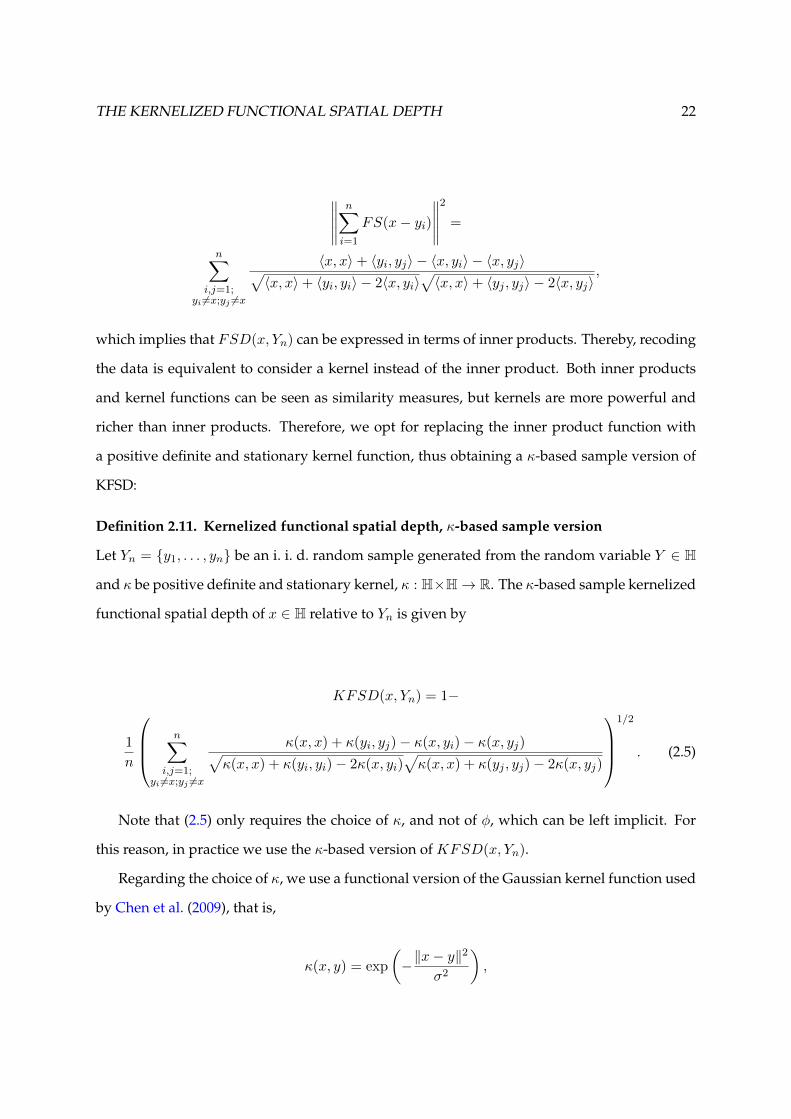
a positive definite and stationary kernel function, thus obtaining a κ-based sample version of

KFSD:

Definition 2.11. Kernelized functional spatial depth, κ-based sample version

Let Yn = y1, . . . , yn be an i. i. d. random sample generated from the random variable Y ∈ H

and κ be positive definite and stationary kernel, κ : H×H→ R. The κ-based sample kernelized

functional spatial depth of x ∈ H relative to Yn is given by

KFSD(x, Yn) = 1−

1

n

n∑i,j=1;

yi 6=x;yj 6=x

κ(x, x) + κ(yi, yj)− κ(x, yi)− κ(x, yj)√κ(x, x) + κ(yi, yi)− 2κ(x, yi)

√κ(x, x) + κ(yj , yj)− 2κ(x, yj)

1/2

. (2.5)

Note that (2.5) only requires the choice of κ, and not of φ, which can be left implicit. For

this reason, in practice we use the κ-based version of KFSD(x, Yn).

Regarding the choice of κ, we use a functional version of the Gaussian kernel function used

by Chen et al. (2009), that is,

κ(x, y) = exp

(−‖x− y‖

2

σ2

),


which in turn depends on the norm inherited by the functional Hilbert space where data are as-

sumed to lie and on the bandwidth σ. With the aim of exploring the behavior of κ as a function

of bandwidth, we consider different values of σ. We set each σ equal to the p% percentile of

the empirical distribution of ‖yi − yj‖, yi, yj ∈ Yn. Note that the lower p, the lower σ and the

more local the approach of KFSD. Indeed, with low percentiles KFSD considers small neigh-

borhoods and can be viewed as a potential functional density estimator, whereas with high

percentiles KFSD considers wide neighborhoods and behaves almost as a global depth. There-

fore, the use of different percentiles allows us to cover different degrees of KFSD-based local

approaches. For example, the 10%, 50% and 90% percentiles lead to strongly, moderately and

weakly local approaches, respectively. In the corresponding chapters, we present two methods

to choose a final value of σ in supervised classification and outlier detection problems.

After recalling the definitions of FMD, HMD, RTD, IDD, MBD and FSD, and after present-

ing KFSD, we dedicate the next section to discuss the differences between global and local

depths.

2.5 From Global to Local Depths

The definition of FSD(x, Yn) given by (2.3) allow us to discuss an important feature of FSD,

that is, its global approach to the depth problem, and to show how a local approach is an alter-

native. The functional spatial depth of x relative to Yn depends on the values of the functional

spatial sign function, FS(x−yi), i = 1, . . . , n. Each FS(x−yi) is a unit-norm curve representing

the direction from x to y. Therefore, FSD(x, Yn) depends equally on n directions. This feature

generates a trade-off: on one side, FSD(x, Yn) turns out to be robust to the presence of outliers

in Yn; on the other side, FSD(x, Yn) transforms (x − yi) into a unit-norm curve regardless of

yi being a neighboring or a distant curve from x. For this reason, we describe FSD as a global-

oriented depth since it makes depend the depth of x on the whole Yn, and with equal weights.

However, in some circumstances it may be useful an analysis of narrow neighborhoods of x

and to give more weight to close than distant curves, in other words, to have a local approach


to the depth problem that allow the information brought by yi to depend on the value of a

certain distance between x and yi, as it happens with KFSD.

To illustrate the differences between a global and a local approach to the depth problem, we

show two examples where the goal is to obtain a center-outward ordering of functional data.

We consider five global depths (FMD, RTD, IDD, MBD and FSD) and two local depths (HMD

and our proposal KFSD). In the first example, we generated 21 curves from a given process

and divided them in three groups with 10, 10 and 1 curves, respectively. Then, we added a

different constant curve to each group (the constants are 0, 10 and 5, respectively), obtaining

the curves at the top of Figure 2.1. Afterwards, we computed the depth values of all the curves

using the five global-oriented depths and we observed that according to all the global depths

the highest depth value is attained at the curve of the third group.

0.0 0.2 0.4 0.6 0.8 1.0

05

1015

0.0 0.2 0.4 0.6 0.8 1.0

01

23

45

Figure 2.1: Two functional datasets that we use to show the differences betweenglobal and local depths

The structure of the dataset of the second example is similar, but we used different trans-

formations to obtain the curves belonging to the second and third group (see the plot at the

bottom of Figure 2.1). Also in this case, we observed that according to all global depths the


curve of the third group turns out to be the deepest one. Clearly, both examples involve three

strongly different classes of curves. Nevertheless, when we treat the curves of each example as

belonging to a homogeneous sample, we observe rather inconvenient behaviors of the global

depths. In the two examples, the curve in the third group is roughly in the geometric center of

the dataset, but it is far from the remaining curves and it would be more reasonable to observe

a low depth value at this curve. Actually, this happens with the local depths HMD and KFSD,

and mainly because these depths reduce the contribution of distant curves to the depth value

of a given curve. Indeed, in both examples HMD and KFSD assigned the lowest depth value

to the curves belonging to the third group. This peculiar behavior of HMD and KFSD is due

to their local approach to the depth problem.

Additionally, we also want to give an idea of the potential usefulness of local depths in

ranking correctly outliers that contaminate a functional sample, but that are somehow graph-

ically hidden. To illustrate this fact, we present the following examples: first, we generated

10 datasets of size 50 from a mixture of two stochastic processes, one for normal curves and

one for outliers that are graphically clear, with the probability that a curve is an outlier equal

to 0.05. Second, we generated another group of 10 datasets from a different mixture which

produces outliers that are instead graphically faint. In Figure 2.2 we report a contaminated

dataset for each mixture.

Let nout,j , j = 1, . . . , 10, be the number of outliers generated in the jth dataset. For each

dataset and functional depth, it is desirable to assign the nout,j lowest depth values to the nout,j

generated outliers. For both mixtures and each generated dataset, we registered how many

times the depth of an outlier is indeed among the nout,j lowest values. As depth functions, we

considered the five global depths and two local depths mentioned above. The results reported

in Table 2.1 show that for all the functional depths the ranking of clear outliers is an easier task

than the ranking of faint outliers.

However, while the ranking of clear outliers is reasonably good in different cases, e.g., local

KFSD (100%) or global RTD (95%), the ranking of faint outliers is markedly better with local

depths, i.e., HMD and KFSD (both 76.19%). These results give an idea of the potential of local


0.0 0.2 0.4 0.6 0.8 1.0

−20

24

68

clear contamination

0.0 0.2 0.4 0.6 0.8 1.0

−20

24

68

faint contamination

Figure 2.2: Examples of contaminated datasets: clear contamination (top) and faintcontamination (bottom). The solid curves are normal curves and the dashed curvesare outliers

Table 2.1: Percentages of times a depth assigns avalue among the nout,j lowest ones to an outlier.Types of outliers: clear and faint

type of depths global depths local depthsdepths FMD RTD IDD MBD FSD HMD KFSDclear outliers 85.00 95.00 70.00 60.00 60.00 85.00 100.00faint outliers 0.00 28.57 38.10 14.29 33.33 76.19 76.19


depths in detecting correctly faint outliers.

Finally, we present a comparative example to evaluate the rankings associated to KFSD and

the other functional depths (FMD, HMD, RTD, IDD, MBD and FSD). We used the 54 growth

curves already reported in Figure 1.1 as functional sample Yn. We computed their depth val-

ues using KFSD with a strongly local percentile (i.e., 10%), as well as using the remaining

functional depths. Then, for each depth we obtained Y(n), that is, the depth-based ordered ver-

sion of Yn, and therefore the ranks of the curves (the curve with rank equal to 1 is the deepest

curve, and so forth). We compared the different rankings and we summarized these compar-

isons in Figure 2.3. For example, the figure at the top on the left of Figure 2.3 compares the

KFSD-based ranks (horizontal axis, in an increasing order) with the FMD-based ranks (in the

vertical axis).

0 10 20 30 40 50

010

2030

4050

KFSD vs FMD

0 10 20 30 40 50

010

2030

4050

KFSD vs HMD

0 10 20 30 40 50

010

2030

4050

KFSD vs RTD

0 10 20 30 40 50

010

2030

4050

KFSD vs IDD

0 10 20 30 40 50

010

2030

4050

KFSD vs MBD

0 10 20 30 40 50

010

2030

4050

KFSD vs FSD

Figure 2.3: Comparison of depth-based rankings (KFSD versus FMD, HMD, RTD,IDD, MBD and FSD) using the 54 growth curves of Figure 1.1

Observing Figure 2.3, it is possible to make some remarks:

• The KFSD-based ranking is rather different from the other rankings. However, it seems

that HMD and FSD are the closest depth in terms of ranking similarities. This result is


not surprising since HMD is also a local depth, whereas FSD is the global counterpart of

KFSD.

• The KFSD-based median, that is, the curve with rank equal to 1 according to KFSD, is

not the median for any other depth. On the contrary, all the depths agree on which is the

least deep curve, that is, the curve with rank equal to 54.

We also evaluated different KFSD-based local approaches, As mentioned above, to set σ

in KFSD we consider different percentiles of ‖yi − yj‖, yi, yj ∈ Yn. For example, looking at

the 10%, 50% and 90% percentiles it is possible to evaluate if strongly, moderately and weakly

KFSD-based local approaches differ among them. Using the same functional dataset, we did

this comparison, which is reported in Figure 2.4. The figure at the top of Figure 2.4 compares

the KFSD-based ranks using the 10% percentile (horizontal axis, in an increasing order) with

the case of the 50% percentile (in the vertical axis), while at the bottom the comparison is with

the case of the 90% percentile.

0 10 20 30 40 50

010

2030

4050

KFSD 10% vs 50%

0 10 20 30 40 50

010

2030

4050

KFSD 10% vs 90%

Figure 2.4: Comparison of KFSD-based rankings (percentile 10% versus 50% and90%) using the 54 growth curves of Figure 1.1


Observing Figure 2.4, it is possible to appreciate that the different percentiles generate dif-

ferent rankings. Therefore, the way how to choose an appropriate percentile for KFSD is an

issue to take into account, as indeed we do in the rest of the thesis.

2.6 Conclusions

In this chapter we introduced the kernelized functional spatial depth, a local-oriented and

kernel-based version of the functional spatial depth recently proposed by Chakraborty and

Chaudhuri (2014). Originally developed by Chaudhuri (1996) and Serfling (2002) in the multi-

variate context, the spatial approach allows both FSD and KFSD to study the degree of central-

ity of curves from a new point of view with respect to the other existing functional depths. The

main novelty introduced by KFSD consists in the fact that it addresses the study of functional

datasets at a local spatial level, whereas FSD is more appropriate for global spatial analyses.

For example, by means of two illustrative examples, we showed the potential of KFSD in

analyzing functional samples that deviate from unimodality or in ranking correctly outliers

graphically hidden.

As we showed in Section 2.4, KFSD and FSD are related: KFSD(x, P ) = FSD(φ(x), Pφ),

where φ : H → F is an embedding map, F is a feature space and Pφ is a recoded version of

the probability distribution P . The embedding map φ and the feature space F are implicitly

defined through a positive definite kernel, κ : H×H→ R. This relationship between FSD and

KFSD may represent the basis for the future theoretical study of the properties of KFSD.

KFSD depends on the choice of κ. Another possible future research line consists in the anal-

ysis of some alternatives to the kernel function employed in this thesis. Regarding the κ that

we use at the moment, it depends on its bandwidth σ. To understand the effects of σ on the

behavior of KFSD, we proposed to consider a range of values for σ. This choice allows to cover

different degrees of KFSD-based local approaches, from strongly to weakly local approaches,

and we showed that they may provide different depth rankings. The role and the choice of σ

in classification and outlier detection will be further analyzed in Chapters 3 and 4.

Our nada who art in nada,Nada be thy name.Thy kingdom nada.Thy will be nadain nada as it is in nada.(Ernest Hemingway, A Clean Well Lighted Place)

Chapter 3

Supervised Functional Classification1

3.1 Introduction

In this chapter we use KFSD as a tool to perform supervised functional classification. In gen-

eral, in a supervised functional classification problem there is available a training sample com-

posed of curves belonging to two or more groups and with known class memberships. The

information contained in the training data is then used to assign test curves with unknown

class membership to one of the groups. The analysis of the training information and the con-

struction of the classification rule may be based on the use of a functional depth. Indeed, in this

chapter we consider three existing depth-based procedures to perform supervised functional

classification with simulated and real data. We apply these methods using a battery of func-

tional depths: KFSD, but also FMD, HMD, RTD, IDD, MBD and FSD. We focus on challenging

scenarios in which the differences between groups are not extremely clear-cut or the data may

contain outlying curves. The results that we observe with simulated and real data indicate that

a local KFSD-based approach is a good solution in such setups.

1This chapter is mostly based on the forthcoming article in the journal TEST by Sguera et al. (2014b)available online at http://link.springer.com/article/10.1007/s11749-014-0379-1 or upon request([email protected])

31

SUPERVISED FUNCTIONAL CLASSIFICATION 32

3.2 The Supervised Functional Classification Problem

The natural theoretical framework of supervised functional classification is given by the ran-

dom pair (Y,G), where Y is a functional random variable and G is a categorical random vari-

able describing the class membership. From now on, we assume that G takes values 0 or

1. We also assume to observe a sample of n independent pairs generated from (Y,G), i.e.,

(Yn, Gn) = (y1, g1), . . . , (yn, gn), with n0 observations from the group with label 0 and n1

observations from the group with label 1, n0 + n1 = n, and a curve x with unknown class

membership generated from Y .

Using the information contained in (Yn, Gn), the goal of any supervised functional classi-

fication method is to provide a rule to classify the curve x, and several methods have been

proposed in the literature. For instance, Hastie et al. (1995) have proposed a penalized version

of the multivariate linear discriminant analysis technique, whereas James and Hastie (2001)

have directly built a functional linear discriminant analysis procedure that uses natural cubic

spline functions to model the observations. Using a P-spline approach, Marx and Eilers (1999)

have considered functional supervised classification as a special case of a generalized linear

regression model. Hall et al. (2001) have suggested to perform dimension reduction by means

of functional principal component analysis and then to solve the derived multivariate problem

with quadratic discriminant analysis or kernel methods. Ferraty and Vieu (2003) have devel-

oped a functional kernel-type classifier. Epifanio (2008) have proposed to describe curves by

means of shape feature vectors and to use classical multivariate classifiers for the discrimina-

tion stage. Galeano et al. (2014) have developed new versions of several well known functional

classification procedures which use a semi-distance for functional observations that general-

izes the multivariate Mahalanobis distance. Finally, Biau et al. (2005) and Cerou and Guyader

(2006) have studied some consistency properties of the extension of the k-nearest neighbor

procedure to infinite-dimensional spaces. The first extension considers a reduction of the di-

mensionality of the regressors based on a Fourier basis system, and the second generalization

deals with the real infinite dimension of the spaces under consideration. Note that the k-nearest

neighbor method is indeed a general tool that can be used to perform functional nonparamet-


ric regression, and that classification is a specific case that occurs when the response of the

regression model is categorical (for more details and theoretical results on the general case, see

Burba et al. 2009 and Kudraszow and Vieu 2013).

Besides the above described methods, other alternatives specially designed for datasets

that may contain outlying curves and based on the use of a functional depth have been pro-

posed. Indeed, in Section 3.3 we carry out a simulation study with scenarios that allow outliers,

whereas in Section Section 3.4 we consider two potentially contaminated real datasets. Next,

we report three depth-based proposals:

Definition 3.1. Distance to the trimmed mean method (DTM, Lopez-Pintado and Romo 2006)

Let (Yn, Gn) = (y1, g1), . . . , (yn, gn) be an i. i. d. random sample generated from the random

pair (Y,G) ∈ H × 0, 1 and x a random observation generated from the random variable

Y ∈ H. The distance to the trimmed mean method works as follows:

1. compute the depth-based α-trimmed means µα,g, g = 0, 1;

2. compute dg = ‖x− µα,g‖, g = 0, 1;

3. assign x to the group minimizing dg.

Definition 3.2. Weighted averaged distance method (WAD, Lopez-Pintado and Romo 2006)



Y ∈ H. Denote with Yng =y1g , . . . , yng

the functional sample composed of curves belonging

to group g, g = 0, 1. The weighted averaged distance method works as follows:

1. for a given functional depth, say FD(·, ·), compute the within-group depth values, that

is, FD(yig , Yng

), i = 1, . . . , ng, g = 0, 1. Let wig = FD

(yig , Yng

);

2. compute Wg =∑ng

ig=1

wig‖x−yig‖∑ngig=1 wig

, g = 0, 1;

3. assign x to the group minimizing Wg.


Definition 3.3. Within maximum depth method (WMD, Cuevas et al. 2007)



Y ∈ H. The within maximum depth method works as follows:

1. for a given functional depth, compute the depth values of x relative to Yng , that is,

FD(x, Yng

), g = 0, 1. Let Dg = FD

(x, Yng

);

2. assign x to the group maximizing Dg.

DTM, WAD and WMD can be used together with any functional depth. In the next two

sections we compare the performances of these methods when used in conjunction with alter-

native functional depths such as FMD, HMD, RTD, IDD, MBD, FSD and KFSD. Among the

non-depth-based methods, we consider as benchmark the functional k-nearest neighbor pro-

cedure (k-NN, Cerou and Guyader 2006), which looks at the k nearest neighbors of x in Yn in

terms of the norm of H and assigns x to a group according to the majority vote. It is worth

noting that the classification rule characterizing k-NN makes the method rather robust to the

presence of outliers, and this is the reason why k-NN represents an interesting competitor for

DTM, WAD and WMD.

3.3 Simulation Study

In this chapter and Chapter 2 we have presented three different depth-based classification

procedures (DTM, WAD and WMD) and seven different functional depths (FMD, HMD, RTD,

IDD, MBD, FSD and KFSD). Pairing all the procedures with all the depths, we obtain 21 depth-

based classification methods, plus k-NN. The goal of this section is to compare them through

an extensive simulation study. From now on, we refer to each method by the notation proce-

dure+depth: for example, DTM+FMD refers to the method obtained by using DTM together

with FMD.

We mainly explore the effectiveness of the methods in supervised classification problems


where the appropriate class membership of the curves is hard to be deduced by using graph-

ical tools and/or in scenarios in which outlying curves are allowed. In these cases, it may

happen that the curve we want to classify is geometrically rather central relative to the train-

ing samples of two different groups, but also relatively far from one of them, although not

in an obvious way. In such scenarios, a depth-based classification method may behave better

when used together with a local depth instead of a global depth.

Both methods and depths may depend on some parameters or assumptions. Regarding

the methods, DTM depends on the trimming parameter α, that we set at α = 0.2, as in Lopez-

Pintado and Romo (2006). For the benchmark procedure k-NN, we take k = 5 nearest neigh-

bors since it is a standard choice and the method is reasonably robust with respect to the

parameter k. Regarding the functional depths, for HMD, we follow the recommendations in

Febrero et al. (2008), that is, H is the L2 space, κ(x, y) = (2/√

2π) × exp(−‖x − y‖2/2h2), and

h is equal to the 15% percentile of the empirical distribution of ‖yi − yj‖, i, j = 1, . . . , n.

Note that for WMD+HMD we use a normalized version of HMD to make its range equal to

[0, 1]. For RTD and IDD, we work with 50 projections in random Gaussian directions. For

MBD, we consider bands defined by two curves. For FSD and KFSD, we assume that the

curves lie in the L2 space. Moreover, as introduced in Chapter 2, we consider a set of per-

centiles pk = p1, . . . , pK to set σ in KFSD. In particular, we take K = 7 and pk =

15%, 25%, 33%, 50%, 66%, 75%, 85%.

Next, we describe the structure of our simulation study. We overlook setups in which

curves may be almost well classified by a preliminary graphical analysis and focus on clas-

sification scenarios where the differences among groups are hard to be detected graphically.

Moreover, we allow outliers in one part of the simulation study. We consider two-groups sce-

narios throughout the whole simulation study, that is, g ∈ 0, 1, and xg(s) denotes the curve

generating process for group g.

In absence of contamination, we initially consider two different pairs of curve generating

processes:

1. First pair of curve generating processes (from now on, CGP1) with s ∈ [0, 1]


x0(s) = 4s+ ε(s),

x1(s) = 8s− 2 + ε(s),

where ε(s) is a zero-mean Gaussian component with covariance function given by

E(ε(s), ε(s′)) = 0.25 exp (−(s− s′)2), s, s′ ∈ [0, 1]. (3.1)

2. Second pair of curve generating processes (from now on, CGP2) with s ∈ [0, 2π]

x0(s) = u01 sin s+ u02 cos s,

x1(s) = u11 sin s+ u12 cos s,(3.2)

where u01 and u02 are observations from a continuous uniform random variable between

0.05 and 0.1, whereas u11 and u12 are observations from a continuous uniform random

variable between 0.1 and 0.12.

The main difference between the two processes is that for CGP1 both x0(s) and x1(s) are

composed of deterministic and linear mean functions, plus a random component, while for

CGP2 both x0(s) and x1(s) are exclusively composed of random and nonlinear mean functions.

To allow contamination, we consider the following modified version of CGP1 and CGP2,

where the contamination affects only group 0:

1. First pair of curve generating processes allowing outliers (from now on, CGP1out) with

s ∈ [0, 1]

x0(s) =

4s+ ε(s), with probability 1− q,

4√s+ ε(s), with probability q.

x1(s) = 8s− 2 + ε(s),

where ε(s) is a zero-mean Gaussian component with covariance function given by (3.1)

and 0 < q < 1.


2. Second pair of curve generating processes allowing outliers (from now on, CGP2out) with

s ∈ [0, 2π]

x0(s) =

u01 sin s+ u02 cos s, with probability 1− q,

u01 sin s+ u12 cos s, with probability q.

x1(s) = u11 sin s+ u12 cos s,

where ui,j , i = 0, 1, j = 1, 2 are defined as for CGP2 and 0 < q < 1.

In Figure 3.2 we report a simulated dataset from CGP1, CGP2, CGP1out and CGP2out.

0.0 0.2 0.4 0.6 0.8 1.0

−20

24

6

CGP1

0 1 2 3 4 5 6

−0.1

5−0

.05

0.05

0.10

0.15

CGP2

0.0 0.2 0.4 0.6 0.8 1.0

−20

24

6

CGP1_out

0 1 2 3 4 5 6

−0.1

5−0

.05

0.05

0.10

0.15

CGP2_out

Figure 3.1: Simulated datasets from CGP1, CGP2, CGP1out and CGP2out: eachdataset contains 25 curves from group g = 0 and 25 dashed curves from groupg = 1. For CGP1 and CGP2, the curves from group g = 0 are all noncontaminated(solid). For CGP1out and CGP2out, the curves from group g = 0 can be noncontam-inated (solid) or contaminated (dotted)

Next, we present some details of the simulation study: for each model, we generated 125

replications. For CGP1out and CGP2out, we set the contamination probability q = 0.10. For

each replication, we generated 100 curves, 50 for g = 0 and 50 for g = 1. We used 25 curves

from g = 0 and 25 curves from g = 1 to build each training sample, and we classified the


remaining curves. All curves were generated using a discretized and finite set of 51 equidistant

points between 0 and 1 or 0 and 2π, depending on the model. For all the functional depths, we

used a discretized version of their definitions. We performed the comparison among methods

in terms of misclassification percentages. We report means and standard deviations of the

misclassification percentages in Tables 3.1-3.4.

For what concerns KFSD, since we initially consider the set of percentiles pk to set σ,

for each replication and classification method, we have based the choice of the appropriate

percentile among the 7 options on a cross-validation step. Next, we describe it:

1. We divide each initial training sample in 5 groups-balanced cross-validation test samples,

each one of size 10, and we pair each of them with its natural cross-validation training

sample composed of the remaining 40 curves.

2. Therefore, for a each replication, we have available five pairs of cross-validation training

and test samples. For each classification method and percentile, and for all the pairs, we

classify the curves in the test samples and obtain a misclassification percentage.

3. For each replication and classification method, we search for the minimum misclassifica-

tion percentage and its corresponding percentile, say p∗.

Then, for each replication and classification method, we use exclusively p∗ to set the bandwidth

of KFSD to do classification with the initial pair of training and test samples. In a preliminary

stage of the study, since we observed several ties in the cross-validation step described above,

we used the following second criteria to break the ties:

• for DTM, we select the percentile that minimizes the sum of the distances of the curves

in the cross-validation test samples to the α-trimmed mean of the group at which the

curves belong;

• for WAD, we select the percentile that minimizes the sum of the weighted averaged dis-

tances of the curves in the cross-validation test samples to the group at which the curves

belong;


• for WMD, we select the percentile that maximizes the sum of the scaled KFSD of the

curves in the cross-validation test samples when included in the group at which they

belong.

The second criteria break almost all the ties. However, if after considering the second criterion

a tie is not broken, we break it randomly.

Before showing the results, we discuss some computational issues. Note that for both DTM

and WAD the key step consists in computing the within-group depth values of the training

curves. Hence, we report the computational times (in seconds) that require each functional

depth to perform this task for a training sample of size 50: 0.02 for FMD, 0.08 for HMD, 0.02

for RTD, 0.02 for IDD, less than 0.01 for MBD, 0.05 for FSD, and 0.14 for KFSD2. Additionally,

a 7-percentiles KFSD analysis takes 0.54 seconds, and a 7-percentiles KFSD analysis combined

with a 5-subsamples cross-validation step takes 1.70 seconds. Therefore, the computation of

KFSD is widely feasible, and the option of searching for an appropriate percentile by means of

a cross-validation does not cause major computational problems, whereas it will bring some

classification benefits.

Tables 3.1-3.4 report the performances observed with the data generated from CGP1, CGP2,

CGP1out and CGP2out. Regarding the KFSD-based methods, for each pair of initial training and

test samples and classification method, it may happen to observe the same misclassification

error using the 7 different percentiles. In such cases, the cross-validation step turns out to be

unnecessary. On the contrary, the cross-validation is required if there are at least two different

misclassification errors. For this reason, for each model and method, in Table 3.5 we report the

percentages of replications where the KFSD cross-validation step is required. In the same table

we also report the best performing percentiles for the pairs of initial training and test samples

since this information permits to identify the type of local analysis that would classify best

each type of data.

2For FMD, HMD, RTD and IDD we have used the corresponding R functions that are available in the R packagefda.usc on CRAN (Febrero and Oviedo de la Fuente 2012); for MBD we have followed the guidelines contained inSun et al. (2012); for FSD and KFSD we have built some functions for R, which are available upon request. Featuresof the workstation: Intel Core i7-3.40GHz and 16GB of RAM.


Table 3.1: CGP1. Means and standard deviations (in parenthesis) of the mis-classification percentages for DTM, WAD and WMD-based methods and k-NN

Method/Depth FMD HMD RTD IDD MBD FSD KFSD

DTM0.16 0.22 0.14 0.14 0.18 0.19 0.14

(0.65) (0.73) (0.58) (0.63) (0.62) (0.64) (0.58)

WAD0.10 0.16 0.11 0.11 0.08 0.13 0.10

(0.50) (0.60) (0.53) (0.53) (0.47) (0.55) (0.50)

WMD15.09 1.66 21.90 18.06 11.82 3.30 0.13(5.43) (2.46) (6.82) (6.27) (4.95) (2.89) (0.66)

k-NN0.11

(0.46)



DTM2.43 2.59 2.40 2.45 2.45 2.42 2.35

(2.01) (2.24) (2.00) (2.05) (1.98) (1.99) (2.10)

WAD3.38 3.33 3.10 3.22 3.20 3.02 3.14

(2.32) (2.35) (2.25) (2.33) (2.23) (2.19) (2.25)

WMD0.10 2.16 1.12 0.99 0.13 0.14 0.11

(0.43) (2.75) (1.99) (1.75) (0.49) (0.52) (0.53)

k-NN0.88

(1.53)

Table 3.3: CGP1out. Means and standard deviations (in parenthesis) of the mis-classification percentages for DTM, WAD and WMD-based methods and k-NN


DTM0.11 0.08 0.08 0.08 0.06 0.11 0.05

(0.46) (0.39) (0.39) (0.39) (0.35) (0.46) (0.31)

WAD0.06 0.06 0.06 0.08 0.06 0.06 0.06

(0.35) (0.35) (0.35) (0.39) (0.35) (0.35) (0.35)

WMD14.46 2.34 22.93 18.93 11.47 3.26 0.08(5.54) (2.97) (6.92) (7.11) (5.02) (2.80) (0.39)

k-NN0.08

(0.39)

Table 3.4: CGP2out. Means and standard deviations (in parenthesis) of the mis-classification percentages for DTM, WAD and WMD-based methods and k-NN


DTM3.87 4.11 3.84 3.81 3.76 3.74 3.71

(2.86) (3.11) (2.84) (2.75) (2.86) (2.83) (2.91)

WAD4.94 4.94 4.67 4.74 4.80 4.48 4.70

(3.36) (3.44) (3.25) (3.25) (3.24) (3.16) (3.29)

WMD0.82 2.90 4.19 3.84 0.83 0.83 0.58

(1.48) (3.31) (3.72) (3.26) (1.55) (1.46) (1.29)

k-NN1.97

(2.05)


Table 3.5: DTM+KFSD, WAD+KFSD and WMD+KFSD, and curve generatingprocesses CGP1, CGP2, CGP1out and CGP2out: percentages of the replicationsfor which cross-validation is required and best performing percentiles for theinitial training and test samples

Model Method Percentage Percentiles Model Method Percentage Percentiles

CGP1DTM 7.20 50%

CGP2DTM 21.60 66%

WAD 2.40 15%, 25%, 50%, 66%, 75% WAD 13.60 85%WMD 56.00 50%, 66%, 75% WMD 12.80 66%, 85%

CGP1outDTM 3.20 15%, 25%, 50%, 66%

CGP2outDTM 26.40 85%

WAD 0.00 all WAD 19.20 85%WMD 58.40 66% WMD 37.60 75%

The results in Tables 3.1-3.5 show that:

1. When the curves are generated from CGP1 or CGP1out, WAD is the best classification

procedure, but also the performances of DTM are competitive. Both procedures turn

out rather stable with respect to the choice of the functional depth. On the contrary,

WMD is more sensitive to the choice of the depth measure, and only the combination

WMD+KFSD is able to compete with WAD and DTM. The performances of k-NN are

quite good, but they are not the best ones neither for CGP1 nor for CGP1out. Indeed, for

CGP1, the best method is WAD+MBD (0.08%), whereas WAD+KFSD and WAD+FMD are

the second best methods (0.10%). For CGP1out, the best method is DTM+KFSD (0.05%),

and some other spatial depth-based methods perform also quite good, e.g., WAD+FSD

and WAD+KFSD (0.06%). Finally, note that WMD+KFSD behaves reasonably well in

both scenarios (0.13% with CGP1 and 0.08% with CGP1out).

2. When the curves are generated from CGP2 or CGP2out, WMD, in conjunction with FMD,

MBD, FSD and KFSD, is clearly the best performing classification procedure: indeed,

the four resultant methods markedly outperform k-NN. For CGP2, the best method is

WMD+FMD (0.10%), but the performance of WMD+KFSD is almost equal (0.11%). For

CGP2out, the best method is clearly WMD+KFSD (0.58%).

3. The cross-validation step is in general required more by WMD+KFSD, and to a smaller

extent by DTM+KFSD, and finally by WAD+KFSD. For example, with CGP1out the cross-

validation step is completely unnecessary for WAD+KFSD, whereas it is advisable for


more than one-half of the replications with WMD+KFSD. On the other hand, looking at

the best performing percentiles and focusing on the methods highlighted in the previous

two points, we observe the following: under CGP1 and CGP1out, WAD+KFSD reaches

its best performances with several percentiles; under CGP2 and CGP2out, the best perfor-

mances of WMD+KFSD are with rather high percentiles. This last result is coherent with

the good performances of WMD+FSD under CGP2 and CGP2out. Indeed, the higher is

the percentile, the less local-oriented is KFSD, and its behavior tends towards the behav-

ior of FSD, its global-oriented counterpart.

Observing the curves generated from CGP1 in Figure 3.1, it is possible to appreciate a rather

strong data dependence structure due to the covariance function given by (3.1). On the other

hand, observing the curves generated from CGP2 at any fixed s ∈ [0, 2π], a low data variability

stands out. We enhance our simulation study by relaxing these two features of CGP1 and CGP2

and considering two modifications of them. First, we consider a variation of CGP1 (from now

on, CGP3) which consists in substituting the covariance function of the additive zero-mean

Gaussian component previously given by (3.1) with a weaker version defined by

E(ε(s), ε(s′)) = 0.30 exp (−|s− s′|/0.3), s, s′ ∈ [0, 1].

Second, we consider a variation of CGP2 (from now on, CGP4) which consists in adding to the

two processes in (3.2) two identical additive zero-mean Gaussian components having covari-

ance function

E(ε(s), ε(s′)) = 0.00025 exp (−(s− s′)2), s, s′ ∈ [0, 2π].

Figure 3.2 reports two simulated datasets from CGP3 and CGP4.

We use CGP3 and CGP4 to develop the third and last part of the simulation study. Tables

3.6 and 3.7 report the performances of the 21 depth-based methods and of k-NN, whereas

Table 3.8 is the analogous of Table 3.5 for CGP3 and CGP4.



0.0 0.2 0.4 0.6 0.8 1.0

−4−2

02

46

CGP3

0.0 0.2 0.4 0.6 0.8 1.0

−0.1

0.0

0.1

0.2 CGP4

Figure 3.2: Simulated datasets from CGP3 and CGP4: each dataset contains 25 solidcurves from group g = 0 and 25 dashed curves from group g = 1



DTM1.33 1.36 1.39 1.36 1.36 1.38 1.31

(1.39) (1.40) (1.44) (1.47) (1.31) (1.42) (1.35)

WAD1.14 1.18 1.20 1.17 1.17 1.20 1.17

(1.33) (1.32) (1.37) (1.35) (1.32) (1.34) (1.32)

WMD5.26 2.93 17.42 14.64 4.29 1.44 1.20

(3.12) (2.66) (5.90) (5.51) (2.76) (1.56) (1.39)

k-NN1.39

(1.46)



DTM2.38 2.53 2.30 2.38 2.26 2.30 2.26

(2.61) (2.59) (2.46) (2.47) (2.42) (2.45) (2.40)

WAD3.55 3.46 3.46 3.46 3.60 3.36 3.41

(3.08) (3.08) (2.87) (2.98) (3.07) (2.92) (2.94)

WMD15.52 2.88 28.54 24.02 12.96 4.90 0.82(5.29) (3.19) (6.99) (6.98) (4.76) (3.96) (1.57)

k-NN1.81

(2.28)


Table 3.8: DTM+KFSD, WAD+KFSD and WMD+KFSD, and curve generatingprocesses CGP3 and CGP4: percentages of the replications for which cross-validation is required and best performing percentiles for the initial trainingand test samples

Model Method Percentage Percentiles Model Method Percentage Percentiles

CGP3DTM 12.00 25%, 75%, 85%

CGP4DTM 14.40 85%

WAD 0.80 25%, 33%, 50%, 66%, 75% WAD 7.20 66%WMD 28.00 75%, 85% WMD 77.60 33%

1. When the curves are generated from CGP3, which is a modification of CGP1, we observe

similar results. WAD is the best classification procedure, but the behavior of DTM is

not bad at all. WMD heavily fails, with the exceptions of the spatial depths KFSD and

FSD, and HMD. k-NN is a competitive classification procedure, but all the DTM and

WAD-based methods, and WMD+KFSD outperform it. The best method is WAD+FMD

(1.14%), whereas there are several best second methods (1.17%), including WAD+KFSD.

2. When the curves are generated from CGP4, which is a modification of CGP2, we observe

that WMD+KFSD is the only method able to outperform k-NN (0.82% against 1.81%),

whereas the remaining methods highlighted for CGP2, i.e., WMD+FMD, WMD+MBD

and WMD+FSD, drastically worsen.

3. As for the previous models, the cross-validation step is in general required more by

WMD+KFSD, and to a smaller extent by DTM+KFSD, and finally by WAD+KFSD. For

example, with CGP3 the cross-validation step is almost unnecessary for WAD+KFSD,

whereas it is advisable for more than one-quarter of the replications with WMD+KFSD.

On the other hand, looking at the best performing percentiles and focusing on the meth-

ods highlighted in the previous two points, we observe that for CGP3 WAD+KFSD

reaches its best performance with all the percentiles except the 15% one, whereas for

CGP4 the best performances of WMD+KFSD are with the 33% percentile, which means

that for this method there is a gain when a rather strong local approach is implemented.

To conclude, we have observed that for the curve generating processes having a deter-

ministic and linear mean function and a random component, i.e., CGP1, CGP1out and CGP3,

WAD+KFSD is among the best and most stable classification methods, and both DTM+KFSD


and WMD+KFSD have performances that are not so different. On the other hand, for the curve

generating processes having a random and nonlinear mean function, i.e., CGP2, CGP2out and

CGP4, WMD+KFSD is clearly the best classification method. Therefore, KFSD-based func-

tional supervised classification is certainly a good option to discriminate curves.

3.4 Real Data Study

To complete the comparison among the depth-based supervised classification methods and

k-NN, we also consider two real datasets.

3.4.1 Growth Data

The first real dataset consists of 93 growth curves: 54 are heights of girls, 39 are heights of

boys. All of them are observed at a common discretized set of 31 nonequidistant ages between

1 and 18 years. Figure 3.3 shows the curves (for more details about this dataset, see Ramsay

and Silverman 2005). We use natural cubic spline interpolation to estimate the growth curves

at a common and equally spaced domain.

This dataset has been analyzed by Lopez-Pintado and Romo (2006) and Cuevas et al. (2007).

From our point of view, these data are interesting mainly for two reasons: first, the differences

between the two groups are not so much sharp; and second, we can not discard the presence

of some outlying curves, especially among girls.

We perform the first part of the growth data classification study with a similar structure to

the simulation study. More precisely, we consider 150 training samples composed of 40 and

30 randomly chosen curves of girls and boys, respectively. We pair each training sample with

the test sample composed of the remaining 14 and 9 curves of girls and boys, respectively. We

denote this way of obtaining training and test samples as T1, and we try to classify the curves

included in each test sample by using the methods and depths considered in Section 3.4, with

the same specifications for both.

For what concerns the cross-validation step for KFSD, we divide each initial training sam-


5 10 15

8010

012

014

016

018

020

0 Girls

5 10 15

8010

012

014

016

018

020

0 Boys

5 10 15

8010

012

014

016

018

020

0 G & B

Figure 3.3: Growth curves: 54 heights of girls (top left), 39 heights of boys (topright), 93 heights of girls and boys (bottom; the dashed curves are boys)

ple in 5 groups-unbalanced cross-validation test samples with 8 and 6 curves of girls and boys,

respectively, and we pair each of them with its natural cross-validation training sample.

We report the performances of the 21 depth-based methods and k-NN in Table 3.9. In Ta-

ble 3.11 we report the percentages of pairs of initial training and test samples for which the

cross-validation step is required by DTM+KFSD, WAD+KFSD and WMD+KFSD, and we also

show the best performing percentiles for the same samples.

Table 3.9: Growth data and T1. Means and standard deviations (in parenthesis)of the misclassification percentages for DTM, WAD and WMD-based methodsand k-NN


DTM15.22 10.84 19.33 19.91 17.30 19.45 12.14(8.18) (7.35) (8.78) (8.99) (8.80) (9.08) (7.82)

WAD14.43 11.22 15.10 15.16 14.87 15.42 12.84(7.56) (7.41) (8.18) (7.88) (8.11) (8.12) (7.48)

WMD30.41 4.96 35.36 33.16 27.59 18.03 3.45

(11.31) (4.56) (8.60) (8.79) (10.22) (7.39) (3.57)

k-NN3.86

(3.56)

Additionally, we consider important to study how the classification methods work when


the goal is to classify a single curve using the information contained in the rest of the curves.

To do this with the growth data, we consider each possible training sample composed of 92

curves, and classify the curve not included in the training set. We denote this way of obtaining

training and test samples as T2, and we implement a cross-validation step for DTM+KFSD,

WAD+KFSD and WMD+KFSD also for T2. We report the performances of the classification

methods under T2 in Tables 3.10 and 3.11.

Table 3.10: Growth data and T2. Number of misclassified curves with DTM,WAD and WMD-based methods and k-NN

Method/Depth FMD HMD RTD IDD MBD FSD KFSDDTM 15 9 17 19 15 18 11WAD 12 10 13 13 13 13 11WMD 28 3 32 30 24 16 2k-NN 3

Table 3.11: Growth data and DTM+KFSD, WAD+KFSD and WMD+ KFSD.Percentages of initial T1-type and T2-type training and test samples for whichcross-validation is required and best performing percentiles for the same sam-ples

T Method Percentage Percentiles T Method Percentage Percentiles

T1DTM 72.00 33%

T2DTM 3.23 25%

WAD 36.67 50% WAD 1.08 50%, 66%WMD 91.33 15% WMD 10.75 15%

The results in Tables 3.9-3.11 show that WMD+KFSD is the only method able to outper-

form k-NN, an occurrence that has been already observed with curves generated from CGP4.

Indeed, under T1, WMD+KFSD outperforms k-NN in terms of means of the misclassification

percentages (3.45% against 3.86%), whereas the third best method is WMD+HMD (4.96%);

something similar happens under T2: WMD+KFSD misclassifies 2 curves, and it is still the best

method, followed by k-NN and WMD+HMD, which misclassify 3 curves. If we convert these

T2 performances in percentages, i.e.,(

#misclassified curvessample size × 100

), we observe that, moving

from T1 to T2, there is a slight but systematic improvement: WMD+KFSD, 3.45% → 2.16%;

k-NN, 3.86%→ 3.23%; WMD+HMD, 4.96%→ 3.23%. This pattern is due to the greater size of

the training samples under T2, but it does not cause significant changes in the performances-

based order of the methods.

For what concerns the cross-validation step of the KFSD-based classification methods, most


of the remarks made for the simulated data also hold for this dataset. Moreover, it is clear that

the implementation of the cross-validation step is a key issue under T1, whereas it becomes

much less important under T2. Finally, under both T1 and T2, the best performing percentile

for the best method, i.e., WMD+KFSD, is the 15% percentile, which means that classification

of growth curves requires a strongly local approach.

Even though here we do not show the results obtained with the 7 different percentiles,

we would like to report that, when we combine WMD with KFSD and use a fixed percentile,

higher percentiles make the performances of the classification method worse. For example, us-

ing WMD and KFSD with the 15% and the 25% percentile, under T1 we observe means equal

to 3.68% and 4.70%, respectively, whereas under T2 the methods misclassify 3 and 4 curves,

respectively. Given the results under T2, we look at the misclassified curves by these two

versions of WMD+KFSD and k-NN: using the 15% percentile, WMD+KFSD misclassifies girls

with labels 11, 25 and 49; using the 25% percentile, it misclassifies girls with labels 8, 25, 49 and

38; k-NN misclassifies girls with labels 8, 25 and 49 (see Figure 3.4).

5 10 15

8010

012

014

016

018

020

0

Growth data

Age(years)

Hei

ght(c

m)

Girls

Boys

Girl 8

Girl 11

Girl 25

Girl 38

Girl 49

Figure 3.4: Growth curves: highlighting some interesting curves for the classifica-tion problem


Therefore, the differences between WMD+KFSD when used with the 15% percentile and

k-NN lie in girls 8 and 11. Observing these curves, we can appreciate that with a local spatial

approach it is possible to classify correctly a female height having apparently an outlying be-

havior (Girl 8), however at the price of misclassifying a more central female height (Girl 11);

on the contrary, k-NN makes the opposite, and its behavior is more similar to the behavior

of WMD+KFSD when used with the 25% percentile, which misclassifies the same curves as

k-NN, in addition to the girl with label 38. Thanks to the cross-validation step, which allows

a non-fixed percentile, WMD+KFSD takes advantage of the differences between the use of the

15% and the 25% percentile, and it succeeds in misclassifying only girls with labels 25 and 49.

3.4.2 Phoneme Data

The second real dataset that we consider consists in log-periodograms of length 150 corre-

sponding to recordings of speakers pronouncing the phonemes “aa” or “ao”. More precisely,

the dataset contains 400 recordings of the phoneme “aa” and 400 recordings of the phoneme

“ao”. Since we are considering a large number of methods, we perform the study using 100

randomly chosen recordings of the phoneme “aa” (from now on, AA curves) and 100 ran-

domly chosen recordings of the phoneme “ao” (from now on, AO curves). Figure 3.5 shows

the curves. For more details about this dataset, see Ferraty and Vieu (2006).

Observing Figure 3.5, we can appreciate similar features to the ones highlighted for the

growth curves: first, we can not discard the presence of some outlying curves in both groups;

and second, the differences between the two groups are not so much sharp. Indeed, this sec-

ond feature seems exaggerated in the second part of the data (frequencies from 76 to 150), and

the discriminant information seems to lie especially in the first part of them (frequencies from

1 to 75). This hypothesis has been confirmed by a preliminary classification analysis in which

we have observed that in general any method improves its performances when only the first

half of the curves is used. Then, we perform the phoneme data classification study using the

first 75 frequencies, and with a structure that is similar to the one used for the growth data,

that is, we classify curves included in test samples that we obtain by means of both T1 and T2.


0 50 100 150

05

1015

2025

Phoneme data

Frequencies

Log−

perio

dogr

ams

Figure 3.5: Phoneme data: log-periodograms of 100 AA curves (solid) and 100 AOcurves (dashed)

To perform the T1 part of the study, we consider 100 training samples composed of 75 ran-

domly chosen AA curves and 75 randomly chosen AO curves. Each training sample is paired

with the test sample composed of the remaining 25 AA curves and 25 AO curves (i.e., the allo-

cation “150 training curves, 50 test curves” defines T1), and we classify the curves included in

each test sample by using the same methods and depths as in subsection 3.4.1, with the same

specifications for both.

For what concerns the cross-validation step for KFSD, it is similar to the one implemented

for the simulated data, but in this case we divide each initial training sample in 5 groups-

balanced cross-validation test samples of size 30 and we pair each of them with its natural

cross-validation training sample of size 120.

We report the performances of the 21 depth-based methods and k-NN in Table 3.12, whereas

Table 3.14 is the analogous of Table 3.11 for the phoneme data.

To perform the T2 part of the study, we consider all the possible 200 training samples

composed of 199 phonemes, each one jointly with its corresponding test sample composed


Table 3.12: Phoneme data and T1. Means and standard deviations (in paren-thesis) of the misclassification percentages for DTM, WAD and WMD-basedmethods and k-NN


DTM21.56 23.16 22.68 22.70 21.84 23.00 23.08(5.07) (5.64) (5.47) (5.37) (5.18) (5.56) (5.60)

WAD23.12 23.74 23.88 23.84 23.54 23.64 23.36(5.49) (5.82) (5.78) (5.73) (5.60) (5.82) (5.78)

WMD21.42 24.76 26.18 25.62 20.54 20.62 19.30(4.56) (5.50) (5.79) (6.06) (4.57) (4.86) (4.66)

k-NN22.14(5.01)

of the remaining curve. As for the growth data, we implement a cross-validation step for

DTM+KFSD, WAD+KFSD and WMD+KFSD also under T2. We report the performances of the

classification methods under T2 in Tables 3.13 and 3.14.

Table 3.13: Phoneme data and T2. Number of misclassified curves with DTM,WAD and WMD-based methods and k-NN

Method/Depth FMD HMD RTD IDD MBD FSD KFSDDTM 43 46 45 46 44 45 46WAD 46 50 51 52 46 49 46WMD 43 51 50 51 39 39 37k-NN 45

Table 3.14: Phoneme data and DTM+KFSD, WAD+KFSD and WMD+ KFSD.Percentages of initial T1-type and T2-type training and test samples for whichcross-validation is required and best performing percentiles for the same sam-ples

T Method Percentage Percentiles T Method Percentage Percentiles

T1DTM 10.00 25%

T2DTM 0.00 15%, 25%, 33%, 50%, 66%, 75%, 85%

WAD 33.00 15% WAD 1.00 15%, 25%, 33%, 50%, 66%WMD 54.00 15% WMD 1.50 15%, 25%, 33%, 50%, 66%, 75%

The results in Tables 3.12-3.14 show especially two facts: first, classification of phoneme

data is a hard problem, and effectively the number of misclassified curves is large with any

method and under both T1 and T2; second, WMD+KFSD is the best classification method.

Indeed, under T1, WMD+KFSD is the method with the best performance in terms of mean

of the misclassification percentages (19.30%), and it outperforms the second best method,

WMD+MBD (20.54%). The third best method is given by another spatial depth-based method,

WMD+FSD (20.62%). Under T2, WMD+KFSD is again the method with the best performance


(37 misclassified curves), whereas WMD+MBD and WMD+FSD are the second best methods

(39 misclassified curves). Note that the performance of the fourth best method is quite distant

(WMD+FMD, 43 misclassified curves), as well as the one of k-NN (45 misclassified curves).

If we convert the T2 performances of the three best methods in percentages, there is a slight

but systematic improvement when moving from T1 to T2: WMD+KFSD, 19.30% → 18.50%;

WMD+MBD, 20.54%→ 19.50%; WMD+FSD, 20.62%→ 19.50%. However, as for growth data,

we observe no significant changes in the performances-based order of the methods.

Observing Table 3.14 and focusing on the best KFSD-based method, i.e., WMD+KFSD, we

appreciate that under T1 the best performing percentile for WMD+KFSD is the 15% percentile,

whereas for T2 the best performing percentiles for WMD+KFSD are all except the 85% per-

centile. However, even though we do not show the results obtained with the 7 different per-

centiles, we would like to report that for the phoneme data, unlike for the growth data, when

we combine WMD with KFSD and a fixed percentile, even with the worst performing per-

centile, which is the 85% percentile, WMD+KFSD has performances comparable to the best

ones. Indeed, using the 85% percentile, WMD+KFSD still outperforms the second best me-

thod of Table 3.12 (19.90% against 20.54% of WMD+MBD under T1), and it misclassifies the

same number of curves as the second best methods of Table 3.13 (39 misclassified curves by

WMD+MBD and WMD+FSD under T2).

3.5 Conclusions

After presenting KFSD in Chapter 2, in this chapter we focused on supervised functional clas-

sification problems using the depth-based methods DTM, WAD and WMD, and a benchmark

procedure such as k-NN. The three depth-based methods were used together with KFSD, FSD

and five more existing functional depths. We developed a simulation study where the dif-

ferences between curves of different groups are not excessively marked and/or the data may

contain outliers, and we analyzed two real datasets with similar features. In both cases, we

observed that a KFSD-based method is always among the best methods in terms of classifica-


tion capabilities and that it outperforms the benchmark procedure k-NN. Note that no other

depth behaved as well as KFSD, and that WMD+KFSD produced doubtless the most stable

and best depth-based classification method: indeed, WMD+KFSD has always outperformed

WMD+FSD, which is its natural global-oriented competitor, and, more in general, it had ac-

ceptable results and often the best ones, as in the case of growth and phoneme data.

Io so. Ma non ho le prove.Non ho nemmeno indizi.(Pier Paolo Pasolini, Cos’ e questo golpe? Io so)

Chapter 4

Functional Outlier Detection1

4.1 Introduction

The accurate identification of outliers is an important aspect in any statistical data analysis.

Nowadays there are well-established outlier detection techniques in the univariate and multi-

variate frameworks (for a complete review, see for example Barnett and Lewis 1994) as well as

in FDA. The possible reasons why statisticians are interested in identifying outliers are mainly

two: first, any statistical technique may lead to misleading results and conclusions when ap-

plied to contaminated datasets; second, since outliers may arise because of extraordinary de-

viations from the average pattern of the data, a further non-statistical analysis of extreme real-

izations can reveal interesting but latent features of the phenomenon under study.

According to Febrero et al. (2007, 2008), a functional outlier is a curve generated by a sto-

chastic process with a different distribution than the distribution of the normal curves. This

definition covers many types of outliers, e.g., magnitude outliers, shape outliers and partial

outliers, i.e., curves having atypical behaviors only in some segments of the domain. Shape

and partial outliers are typically harder to detect than magnitude outliers (in the case of high

magnitude, outliers can even be recognized by simply looking at a graph), and therefore entail

more difficult outlier detection problems. In this chapter we focus on such scenarios and, from

1This chapter is mostly based on the working paper by Sguera et al. (2014a)

55

FUNCTIONAL OUTLIER DETECTION 56

now on, we refer to low magnitude, shape and partial outliers as “faint outliers” and to high

magnitude outliers as “clear outliers”.

When the local spatial depth KFSD is used to order sample curves from the most to the least

central, in general it succeeds in ranking faint outliers among the least deep curves. To exploit

at the best this feature of KFSD, we introduce three new procedures that provide a threshold

value for KFSD such that curves with depth values lower than the threshold are detected as

outliers: first, we present a result that allows to select a threshold for KFSD to detect outliers.

This result is based on a probabilistic upper bound on a desired false alarm probability of de-

tecting normal curves as outliers. However, its practical application requires the availability

of two samples, circumstance rather uncommon in classical outlier detection problems. Then,

we propose three solutions based on smoothed resampling techniques that require instead a

unique sample.

We study the performances of the resampling-based procedures in a simulation study and

in a real application with environmental data, and we compare them with the performances of

some competitors. First, we consider the methods proposed by Febrero et al. (2008), who also

suggested to label as outliers those curves with depth values lower than a certain threshold: as

functional depths, they considered three alternatives, i.e., FMD, HMD and IDD, whereas, they

proposed two alternative bootstrap procedures based on depth-based trimmed and weighted

resampling, respectively, to determine the depth threshold. Second, we employ the functional

boxplot presented by Sun and Genton (2011). The proposed functional boxplot is constructed

using the ranking of curves provided by MBD and allows to detect outliers as well as the stan-

dard boxplot does. Finally, since the use of a functional depth is only one among the possible

strategies for tackling the functional outlier detection problem, we also consider the methods

proposed by Hyndman and Shang (2010), who first reduce the outlier detection problem from

functional to multivariate data by means of functional principal component analysis (FPCA),

and then use two alternative multivariate techniques on the scores to detect outliers, i.e., the

bagplot and the high density region boxplot, respectively. The results of the comparative study

support our proposals.


4.2 Outlier Detection for Functional Data

The outlier detection problem can be described as follows: let Yn = y1, . . . , yn be a sam-

ple that has been generated from a mixture of two functional random variables in H, one for

normal curves and one for outliers, say Ynor and Yout, respectively. Let Ymix be this mixture,

i.e.,

Ymix =

Ynor, with probability 1− α,

Yout, with probability α,(4.1)

where α ∈ [0, 1] is the contamination probability (usually, a value rather close to 0). The curves

composing Yn are all unlabeled, and the goal of the analysis is to decide whether each curve is

a normal curve or an outlier.

Since any functional depth measures the degree of centrality/extremality of a given curve

relative to a distribution or a sample, outliers are expected to have low depth values. In Chap-

ter 3 we used depth-based methods to solve supervised functional classification problems. It

was observed that a local approach is preferable when the classes involved in the problem are

not extremely different or distant. Here, we show that an approach based on a local depth

such as KFSD also succeeds in detecting faint outliers such as low magnitude, shape or partial

outliers.

Recall that KFSD is a functional extension of the kernelized spatial depth for multivariate

data (KSD) proposed by Chen et al. (2009), who also proposed a KSD-based outlier detector

that we generalize to KFSD: for a given dataset Yn generated from Ymix and t, b ∈ [0, 1], the

KFSD-based outlier detector for x ∈ H is given by

g(x, Yn) =

1, if KFSD(x, Yn) ≤ t,t+b−KFSD(x,Yn)

b , if t < KFSD(x, Yn) ≤ t+ b,

0, if KFSD(x, Yn) > t+ b,

(4.2)

where t is a threshold and b determines the transition rate of x from being an outlier (case

g(x, Yn) = 1) to be a normal curve (case g(x, Yn) = 0). Clearly, (4.2) depends on the values of


t and b. On the one hand, it is desirable a value of t capable of discriminating between x gen-

erated from Ynor or Yout. On the other hand, the role of b depends on the goal of the analysis.

If the options “outlier” and “normal curve” are the only ones of interest, b should be set at 0.

However, if there is interest in further analysis of “potential outliers”, b may be allowed to be

greater than 0. In our case, since the main goal is outlier detection and t is the key parameter

to be set, we let b = 0.

For the multivariate case, Chen et al. (2009) studied KSD-based outlier detection under dif-

ferent scenarios. One of them consists in an outlier detection problem where two samples are

available, and for which they proposed to select the threshold t by controlling the probability

that normal observations are classified as outliers, i.e., the false alarm probability (FAP). They

proved a result providing a KSD-based probabilistic upper bound on the FAP which depends

on t. Then, the maximum value of t such that the upper bound does not exceed a given desired

FAP provides a threshold for KSD. Next, we extend this result to KFSD:

Theorem 4.1. Let YnY = yi, . . . , ynY and ZnZ = zi, . . . , znZ be two i. i. d. samples generated

from the unknown mixture of random variables Ymix ∈ H described by (4.1), with α > 0. Let g(·, YnY )

be the outlier detector defined in (4.2). Fix δ ∈ (0, 1) and suppose that α ≤ r for some r ∈ [0, 1]. For

a new random element x generated from Ynor, the following inequality holds with probability at least

1− δ:

Ex∼Ynor [g(x, YnY )] ≤ 1

1− r

1

nZ

nZ∑i=1

g (zi, YnY ) +

√ln 1/δ

2nZ

, (4.3)

where Ex∼Ynor refers to the expected value with respect to x generated from Ynor.

The proof of Theorem 4.1 is presented in the appendix of this chapter. Recall that the FAP

has been defined as the probability that a normal observation x is classified as outlier. For the

elements of Theorem 4.1, Prx∼Ynor (g(x, YnY ) = 1) is the FAP. If we set b = 0,

Prx∼Ynor (g(x, YnY ) = 1) = Ex∼Ynor [g(x, YnY )] .

Therefore, the probabilistic upper bound of Theorem 4.1 applies also to the FAP.


It is worth noting that the application of Theorem 4.1 requires to observe two samples, cir-

cumstance rather uncommon in classical outlier detection problems, but also a considerably

large nZ . To show the last point, recall that the right-hand side of (4.3) has to be controlled

under the desired FAP and is in practice composed by two addends, with the second equal to

11−r

√ln 1/δ2nZ

. For some normal values such as r = 0.05, δ = 0.05 and nZ = 50, we would have

11−r

√ln 1/δ2nZ

= 0.18, which is greater than a normal desired FAP such as 0.10, and it shows that

the use of Theorem 4.1 may be compromised under some common situations.

We propose three solutions to overcome these limitations. Assume to observe a functional

sample Yn generated from an unknown mixture of random variables Ymix. The goal is to iden-

tify which curves in Yn are outliers, but in this situation there are not available two samples

and Theorem 4.1 cannot be applied. We propose to use Yn as YnY , and to obtain ZnZ by resam-

pling with replacement from Yn. In this way, we also solve the problematic issue related to the

second addend of the right-hand side of (4.3) because it is possible to set nZ as large as needed.

Regarding the resampling procedure to obtain ZnZ , we consider three different schemes, all of

them with replacement. Since we deal with potentially contaminated datasets, besides simple

resampling, we also consider two robust KFSD-based resampling procedures inspired by the

work of Febrero et al. (2008). Then, the three resampling schemes that we consider are:

1. Simple resampling.

2. KFSD-based trimmed resampling: once obtained KFSD(yi, Yn), i = 1, . . . , n, it is possi-

ble to identify the dαTne% of least deep curves, for certain 0 < αT < 1 usually close to

0. These least deep curves are deleted from the sample, and simple resampling is carried

out with the remaining curves.

3. KFSD-based weighted resampling: once obtained KFSD(yi, Yn), i = 1, . . . , n, weighted

resampling is carried out with weights wi = KFSD(yi, Yn).

All the above procedures generate samples with some repeated curves. However, in a pre-

liminary stage of our study we observed that it is preferable to work with ZnZ composed of

curves different among them. To obtain such samples, we add a common smoothing step to


the previous three resampling schemes.

To describe the smoothing step, first recall that each curve in Yn is in practice observed

at a discretized and finite set of domain points, and that the sets may differ from one curve

to another. For this reason, the estimation of Yn at a common set of m equidistant domain

points may be required. Let (yi(s1), . . . , yi(sm)) be the observed or eventually estimated m-

dimensional equidistant discretized version of yi, ΣYn be the covariance matrix of the dis-

cretized form of Yn and γ be a smoothing parameter. Consider a zero-mean Gaussian process

whose discretized form has γΣYn as covariance matrix. Let (ζ(s1), . . . , ζ(sm)) be a discretized

realization of the previous Gaussian process. Consider any of the previous three resampling

procedures and assume that at the jth trial, j = 1, . . . , nZ , the ith curve in Yn has been sampled.

Then, the discretized form of the jth curve in ZnZ would be given by (zj(s1), . . . , zj(sm)) =

(yi(s1) + ζj(s1), . . . , yi(sm) + ζj(sm)), or, in functional form, by zj = yi+ζj . Therefore, combin-

ing each resampling scheme with this smoothing step, we provide three different approximate

ways to obtain ZnZ , and we refer to them as smo, tri and wei, respectively. Then, for fixed δ,

r and desired FAP, the threshold t for (4.2) is selected as the maximum value of t such that the

right-hand side of (4.3) does not exceed the desired FAP. Let t∗ be the selected threshold, which

is then used in (4.2) with b = 0 to compute g (yi, Yn), i = 1, . . . , n. If g (yi, Yn) = 1, yi is detected

as outlier. To summarize, we provide three KFSD-based outlier detection procedures and we

refer to them as KFSDsmo, KFSDtri and KFSDwei depending on how ZnZ is obtained (smo, tri

and wei, respectively; recall that YnY = Yn). As competitors of the proposed procedures, we

consider the methods mentioned in Section Section 4.1 that we next describe.

Sun and Genton (2011) proposed a depth-based functional boxplot and an associated out-

lier detection rule based on the center-outward ordering of the sample curves provided by

MBD. Once obtained the ordering, it is used to define the sample central region, that is, the

smallest band containing at least half of the deepest curves. The non-outlying region is de-

fined inflating the central region by 1.5 times. Curves that do not belong completely to the

non-outlying region are detected as outliers. The original functional boxplot is based on the

use of MBD, but clearly any functional depth can be used. Another contribution of this the-


sis is the study of the performances of the outlier detection rule associated to the functional

boxplot (from now on, FBP) when used together with the battery of functional depths that we

considered in supervised classification.

Febrero et al. (2008) proposed two depth-based outlier detection procedures selecting a

threshold for FMD, HMD or IDD by means of two alternative robust smoothed bootstrap pro-

cedures whose single bootstrap samples are obtained using the above described tri and wei,

respectively. Then, at each bootstrap sample, the 1% percentile of the empirical distribution

of the depth values is obtained, say p0.01. If B is the number of bootstrap samples, B values

of p0.01 are obtained. Each method selects as cutoff c the median of the collection of p0.01 and,

using c as threshold, a first outlier detection is performed. If some curves are detected as out-

liers, they are deleted from the sample, and the procedure is repeated until no more outliers

are found (note that c is computed only in the first iteration). From now on, we refer to these

methods as Btri and Bwei. Also in this case, we evaluate these procedures using all the func-

tional depths considered in Chapter 3.

Finally, we also consider two procedures that are not based on the use of a functional depth

proposed by Hyndman and Shang (2010). Both procedures are based on the first two robust

functional principal components scores and on two different graphical representations of them.

The first proposal is the outlier detection rule associated to the functional bagplot (from now

on, FBG), which works as follows: obtain the bivariate robust scores and order them using

the multivariate halfspace depth HSD. Define an inner region by considering the smallest re-

gion containing at least the 50% of the deepest scores, and obtain a non-outlying region by

inflating the inner region by 2.58 times. FBG detects as outliers those curves whose scores are

outside the non-outlying region. Note that the scores-based regions and outliers allow to draw

a bivariate bagplot, which produces a functional bagplot once it is mapped onto the original

functional space. The second proposal is related to a different graphical tool, the high den-

sity region boxplot (from now on, we refer to its associated outlier detection rule as FHD). In

this case, once obtained the scores, perform a bivariate kernel density estimation. Define the

(1−β)-high density region (HDR), β ∈ (0, 1), as the region of scores with coverage probability


equal to (1 − β). FHD detects as outliers those curves whose scores are outside the (1 − β)-

HDR. In this case, it is possible to draw a bivariate HDR boxplot which can be mapped onto a

functional version, thus providing the functional HDR boxplot.

4.3 Simulation Study

After introducing KFSDsmo, KFSDtri and KFSDwei and their competitors (FBP, Btri, Bwei, FBG

and FHD), in this section we carry out a simulation study to evaluate the performances of

the different methods. Since we employ FBP, Btri and Bwei with seven different functional

depths (FMD, HMD, RTD, IDD, MBD, FSD and KFSD), for them we use the notation proce-

dure+depth: for example, FBP+FMD refers to the method obtained by using FBP together with

FMD.

We consider six models for our simulation study: all of them generate curves according to

the mixture of random variables Ymix described in (4.1). The first three mixture models (MM1,

MM2 and MM3) share Ynor, with curves generated by

y(s) = 4s+ ε(s), (4.4)

where s ∈ [0, 1] and ε(s) is a zero-mean Gaussian component with covariance function given

by

E(ε(s), ε(s′)) = 0.25 exp (−(s− s′)2), s, s′ ∈ [0, 1].

Also the remaining three mixture models (MM4, MM5 and MM6) share Ynor, but, in this case,

the curves are generated by

y(s) = u1 sin s+ u2 cos s, (4.5)

where s ∈ [0, 2π] and u1 and u2 are observations from a continuous uniform random variable

between 0.05 and 0.15.


MM1, MM2 and MM3 differ in their Yout components. Under MM1, the outliers are gener-

ated by

y(s) = 8s− 2 + ε(s),

which produces faint outliers of both shape and low magnitude nature. Under MM2, the

outliers are generated by adding to (4.4) an observation from a N(0, 1), and as result outliers

are more irregular than normal curves. Finally, under MM3, the outliers are generated by

y(s) = 4 exp(s) + ε(s),

which produces curves that are normal in the first part of the domain, but that become expo-

nentially outlying.

Similarly, MM4, MM5 and MM6 differ in their Yout components. Under MM4, the outliers

are generated replacing u2 with u3 in (4.5), where u3 is an observation from a continuous uni-

form random variable between 0.15 and 0.17. This change produces partial low magnitude

outliers in the first and middle part of the domain of the curves. Under MM5, the outliers are

generated by adding to (4.5) an observation from a N(0,(0.12

)2), and as result outliers are more

irregular curves. Finally, under MM6, the outliers are generated by

y(s) = u1 sin s+ exp

(0.69s

2π

)u4 cos s, (4.6)

where u4 is an observation from a continuous uniform random variable between 0.1 and 0.15.

As MM3, MM6 allows outliers that are normal in the first part of the domain and become

outlying with an exponential pattern. In Figure 4.1 we report a simulated dataset with at least

one outlier for each mixture model.

The details of the simulation study are the following: for each mixture model, we generate

100 datasets, each one composed of 50 curves. Two values of the contamination probability α

are considered: 0.02 and 0.05. All curves are generated using a discretized and finite set of 51

equidistant points in the domain of each mixture model ([0, 1] for MM1, MM2 and MM3; [0, 2π]


0.0 0.2 0.4 0.6 0.8 1.0

−20

24

6

MM1

0 1 2 3 4 5 6

−0.2

−0.1

0.0

0.1

0.2

MM4

0.0 0.2 0.4 0.6 0.8 1.0

−10

12

34

5

MM2

0 1 2 3 4 5 6

−0.2

−0.1

0.0

0.1

0.2

MM5

0.0 0.2 0.4 0.6 0.8 1.0

02

46

MM3

0 1 2 3 4 5 6

−0.2

−0.1

0.0

0.1

0.2

MM6

Figure 4.1: Examples of contaminated functional datasets generated by MM1,MM2, MM3, MM4, MM5 and MM6. Solid curves are normal curves and dashedcurves are outliers

for MM4, MM5 and MM6) and the discretized versions of the functional depths are used.

In relation with the methods and the functional depths that we consider in the study, the

specifications that we use are the following:

1. FBP when used with FMD, HMD, RTD, IDD, MBD, FSD and KFSD: regarding FBP, as

reported in Section 4.2, the central region is built considering the 50% deepest curves

and the non-outlying region by inflating by 1.5 times the central region. Regarding the

depths, for HMD, we follow the recommendations in Febrero et al. (2008), that is, H is

the L2 space, κ(x, y) = 2√2π

exp(−‖x−y‖

2

2h2

)and h is equal to the 15% percentile of the

empirical distribution of ‖yi − yj‖, yi, yj ∈ Yn. For RTD and IDD, we work with 50

projections in random Gaussian directions. For MBD, we consider bands defined by two

curves. For FSD and KFSD, we assume that the curves lie in the L2 space. Moreover, in

KFSD we set σ equal to a moderately local percentile (50%) of the empirical distribution

of ‖yi − yj‖, yi, yj ∈ Yn.


2. Btri and Bwei when used with FMD, HMD, RTD, IDD, MBD, FSD and KFSD: γ = 0.05,

B = 100, αT = α. Regarding the depths, we use the specifications reported for FBP.

3. FBG: as reported in Section 4.2, the central region is built considering the 50% deepest

bivariate robust functional principal component scores and the non-outlying region by

inflating by 2.58 times the central region.

4. FHD: β = α.

5. KFSDsmo, KFSDtri and KFSDwei: nY = n = 50 (since YnY = Yn), γ = 0.05, αT = α (only

for KFSDtri), nZ = 6n, δ = 0.05, r = α, desired FAP = 0.10. Moreover, as introduced in

Chapter 2, we consider a set of percentiles pk = p1, . . . , pK to set σ in KFSD. In out-

lier detection, pk = 10k%, k = 1, . . . ,K = 9. The way in which we propose to choose

the most suitable percentile for outlier detection is presented below.

In supervised classification the availability of training curves with known class member-

ships makes possible the definition of some natural procedures to set σ for KFSD, such as

cross-validation. However, in an outlier detection problem it is common to have no informa-

tion whether curves are normal or outliers. Therefore, training procedures are not immediately

available.

We propose to overcome this drawback by obtaining a “training sample of peripheral

curves”, and then choosing the percentile that ranks better the peripheral curves as final per-

centile for KFSD in KFSDsmo, KFSDtri and KFSDwei. Next, we describe the procedure, which

is based on J replications. Let Yn be the functional dataset on which outlier detection has to be

done and let Y(n) =y(1), . . . , y(n)

be the depth-based ordered version of Yn, where y(1) and

y(n) are the curves with minimum and maximum depth, respectively. The steps to obtain a set

of peripheral curves are the following:

1. Let p1, . . . , pK be the set of percentiles in use (in our case, pk = 10k%, k = 1, . . . ,K =

9), and choose randomly a percentile from the set. For the jth replication, j ∈ 1, . . . , J,

denote the selected percentile as pj . From now on, we use J = 20.


2. Using pj , compute KFSDpj (yi, Yn), i = 1, . . . , n, where the notation KFSDpj (·, ·) is

used to describe what percentile is used. For the jth replication, denote the KFSD-based

ordered curves as y(1),j , . . . , y(n),j .

3. Take y(1),j , . . . , y(lj),j , where lj ∼ Bin(n, 1n). Apply the smoothing step described in Sec-

tion 4.2 to these curves. For the smoothing step, we use ΣYn and γ = 0.05. For the jth

replication, denote the peripheral and smoothed curves as y∗(1),j , . . . , y∗(lj),j

.

4. Repeat J times steps 1.-3. to obtain a collection of L =∑J

j=1 lj peripheral curves, say YL

(for an example, see Figure 4.2).

0.0 0.2 0.4 0.6 0.8 1.0

−20

24

6

Figure 4.2: Example of a training sample of peripheral curves for a contaminateddataset generated by MM1 with α = 0.05. The solid and shaded curves are theoriginal curves (both normal and outliers). The dashed curves are the peripheralcurves to use as training sample

Next, YL acts as training sample according to the following steps: for each y∗(i),j ∈ YL,

(i ≤ lj), and pk ∈ p1, . . . , pK, compute KFSDpk(y∗(i),j , Y−(i),j), where Y−(i),j = Yn \y(i),j

.

At the end, aL×K matrix is obtained, sayDLK = dlk l=1,...,Lk=1,...,K

, whose kth column is composed

of the KFSD values of the L training peripheral curves when the kth percentile is employed


in KFSD. Let rlk be the rank of dlk in the vector KFSDpk(y1, Yn), . . . ,KFSDpk(yn, Yn), dlk,

e.g., rlk is equal to 1 (n + 1) if dlk is the minimum (maximum) value in the vector. Let RLK

be the result of this transformation of DLK , and sum the elements of each column, obtaining

a K-dimensional vector, say RK . Since the goal is to assign ranks as lower as possible to the

peripheral curves, choose the percentile associated to the minimum value of RK . When a tie

is observed, we break it randomly.

The comparison among methods is performed in terms of both correct and false outlier

detection percentages, which are reported in Tables 4.1-4.6. To ease the reading of the tables,

for each model and α, we report in bold the 5 best methods in terms of correct outlier detection

percentage (c).2 For each model, if a method is among the 5 best ones for both contamination

probabilities α, we report its label in bold.

Table 4.1: MM1, α = 0.02, 0.05. Correct (c) andfalse (f) outlier detection percentages of FBP, Btri,Bwei, FBG, FHD, KFSDsmo, KFSDtri and KFSDwei

α = 0.02 α = 0.05

c f c fFBP+FMD 44.34 1.23 43.86 0.73FBP+HMD 74.53 0.94 72.81 0.61FBP+RTD 61.32 0.57 63.16 0.31FBP+IDD 55.66 0.61 61.84 0.34FBP+MBD 49.06 1.33 50.44 0.69FBP+FSD 62.26 0.67 61.84 0.40FBP+KFSD 66.04 0.86 74.12 0.44Btri+FMD 0.00 0.92 0.00 1.80Btri+HMD 72.64 1.43 62.28 1.51Btri+RTD 8.49 0.37 14.47 0.40Btri+IDD 12.26 0.39 17.11 0.65Btri+MBD 0.00 0.67 0.00 1.51Btri+FSD 1.89 0.84 5.70 1.22Btri+KFSD 70.75 1.57 57.89 1.49Bwei+FMD 0.00 1.23 0.00 1.53Bwei+HMD 71.70 1.16 46.49 0.57Bwei+RTD 10.38 1.25 7.46 1.17Bwei+IDD 14.15 2.29 14.04 2.62Bwei+MBD 0.00 1.14 0.00 1.30Bwei+FSD 1.89 1.33 3.07 1.17Bwei+KFSD 66.04 0.94 57.02 0.52FBG 100.00 2.27 97.81 2.37FHD 48.11 1.00 73.68 2.77KFSDsmo 89.62 4.50 85.09 2.58KFSDtri 89.62 4.92 92.11 4.40KFSDwei 97.17 9.44 96.93 6.54


α = 0.02 α = 0.05


2In presence of tie, we look at the false outlier detection percentage (f), preferring the method with lower f.



α = 0.02 α = 0.05



α = 0.02 α = 0.05




1. KFSDtri and KFSDwei are always among the 5 best methods, whereas KFSDsmo 10 times

over 12, but when its performance is not among the 5 best, it is neither extremely far from

the fifth method (MM2, α = 0.02: 95.18% against 96.39%; MM3, α = 0.02: 73.79% against

78.63%). The rest of the methods are among the 5 best procedures at most 5 times over

12 (FBP+HMD).

2. Regarding MM5 and MM6, our procedures are clearly the best options in terms of correct

detection (c), and in the following order: KFSDwei, KFSDtri and KFSDsmo. In general, this

pattern is observed overall the simulation study. Note that for MM6 and α = 0.02 we

observe the best relative performances of KFSDsmo, KFSDtri and KFSDwei, i.e., 91.58%,

93.68% and 96.84%, respectively, against 67.37% of the fourth best method (Bwei+HMD),

that is, we observe differences greater than 20%, and approaching 30% if KFSDwei and

Bwei+HMD are compared.

3. About MM3, KFSDwei is clearly the best method in terms of correct detection, however

at the price of having a greater false detection (f). This is in general the main weak point

of KFSDsmo, KFSDtri and KFSDwei. As for correct detection, we observe a overall pattern

in our methods in false detection, but in an opposite way, indicating therefore a trade-

off between c and f. Relative high false detection percentages are however something

expected in KFSDsmo, KFSDtri and KFSDwei since these methods are based on the defini-

tion of a desired false alarm probability, which is equal to 10% in this study. Concerning

MM2, we observe similar results to MM3, but in this case the performances of the best

competitors for KFSDwei, i.e., KFSDsmo, KFSDtri, FBP-based methods and Btri and Bwei

when used with local depths, are closer to the results of KFSDwei.

4. Finally, there are only 3 cases in which a competitor outperforms our best method: for

MM1 and both α the best method is FBG, whereas for MM4 and α = 0.05 the best me-

thod is Bwei+IDD. However, both FBG and Bwei+IDD do not show behaviors as stable as


KFSDsmo, KFSDtri and KFSDwei do. Indeed, they show poor performances under other

scenarios, e.g., MM2, MM5 or MM6.

In Figure 4.3 we report a series of boxplots summarizing which percentiles have been se-

lected in the training steps for KFSDsmo, KFSDtri and KFSDwei.

MM

1, 0

.02

MM

1, 0

.05

MM

2, 0

.02

MM

2, 0

.05

MM

3, 0

.02

MM

3, 0

.05

MM

4, 0

.02

MM

4, 0

.05

MM

5, 0

.02

MM

5, 0

.05

MM

6, 0

.02

MM

6, 0

.05

perc

entil

es

1

2

3

4

5

6

7

8

9

Figure 4.3: Boxplots of the percentiles selected in the training steps of the simula-tion study for KFSDsmo, KFSDtri and KFSDwei

Observing Figure 4.3, the following general remarks can be done. First, MM6 is the mixture

model for which lower percentiles have been selected, and it is also the scenario in which our

methods considerably outperform their competitors. The need for a more local approach for

MM6-data may explain the two observed facts about this mixture model. Second, lower and

more local percentiles have been chosen for mixture models with nonlinear mean functions

(MM4, MM5 and MM6) than for mixture models with linear mean functions (MM1, MM2 and

MM3). Finally, the percentiles selected by means of the proposed training procedure seem to

vary among datasets. However, except for MM3 and α = 0.02, at least for half of the datasets

a percentile not greater than the median has been chosen, which implies at most a moderately

local approach.


4.4 Real Data Study: Nitrogen Oxides (NOx) Data

Besides simulated data, we consider a real dataset which consists in nitrogen oxides (NOx)

emission level daily curves measured every hour close to an industrial area in Poblenou

(Barcelona). The dataset is available in the R package fda.usc (Febrero and Oviedo de la

Fuente 2012) and outlier detection on these data has been first performed by Febrero et al.

(2008) in the paper where Btri and Bwei were presented. We enhance their study by consider-

ing more methods and depths.

According to Febrero et al. (2008), NOx are one of the most important pollutants, and it

is important to identify outlying trajectories because these curves may both compromise any

statistical analysis and be of special interest for further analysis.

More in details, the NOx levels were measured in µg/m3 every hour of every day for the

period 23/02/2005-26/06/2005, but only for 115 days was possible to measure the NOx at ev-

ery hour. These 115 curves are the ones composing the final NOx dataset. However, since the

NOx dataset clearly includes working as well as nonworking day curves, following Febrero

et al. (2008), it is more appropriate to consider two different datasets, that is, a sample of 76

working day curves (from now on, W) and another of 39 nonworking day curves (from now

on, NW). Both W and NW are showed in Figure 4.4: at first glance, it seems that each dataset

may contain outliers, especially partial outliers.

Therefore, because of the possible presence of faint outliers, a local depth approach by

means of the use of KFSDsmo, KFSDtri and KFSDwei may be a good strategy to detect outliers.

Besides them, we do outlier detection with all the methods used in Section 4.3. For all the

procedures we use the same specifications as in Section 4.3, and we assume α = 0.05. For

each method, we report the labels of the curves detected as outliers in Table 4.7, whereas in

Figure 4.5 we highlight these curves.

For what concerns W, most of the methods detect as outlier day 37, which apparently shows

a partial outlying behavior before noon and at the end of the day. Another day detected as

outlier by many methods is day 16, whose curve is the one with the highest morning peak.

In addition to curves 16 and 37, KFSDsmo detects as outlier curve 14, as other nine methods


0 5 10 15 20

010

020

030

040

0

W

0 5 10 15 20

010

020

030

040

0

NW

Figure 4.4: NOx data: working (top) and non working (bottom) day curves.

Table 4.7: NOx data, W and NW datasets. Curvesdetected as outliers by FBP, Btri, Bwei, FBG, FHD,KFSDsmo, KFSDtri and KFSDwei

w days non w daysdetected outliers

FBP+FMD - -FBP+HMD 12, 16, 37 5, 7, 20, 21FBP+RTD 37 20FBP+IDD - 5, 7, 20FBP+MBD - -FBP+FSD 37 -FBP+KFSD 12, 16, 37 5, 7, 20, 21Btri+FMD 16, 37 7Btri+HMD 14, 16, 37 7, 20Btri+RTD 14, 16, 37 -Btri+IDD 11, 14, 16, 37 -Btri+MBD 16, 37 7Btri+FSD 14, 16, 37 -Btri+KFSD 12, 14, 16, 37 7, 20Bwei+FMD 16 7Bwei+HMD 16, 37 7, 20Bwei+RTD 14, 16, 37, 38 -Bwei+IDD 16, 37 -Bwei+MBD 16 7Bwei+FSD 16, 37 -Bwei+KFSD 16, 37 7, 20FBG 16, 37 -FHD 12, 14, 16, 37 7, 20KFSDsmo 14, 16, 37 7, 20, 21KFSDtri 12, 14, 16, 37 7, 20, 21KFSDwei 11, 12, 13, 14, 15, 16, 37, 38 7, 20, 21


0 5 10 15 20

010

020

030

040

0

W

11: WE, 09/03/200512: FR, 11/03/200513: TU, 15/03/200514: WE, 16/03/200515: TH, 17/03/200516: FR, 18/03/200537: FR, 29/04/200538: MO, 02/05/2005

0 5 10 15 20

050

100

150

200

250

NW

5: SA, 12/03/2005 7: SA, 19/03/200520: SA, 30/04/200521: SU, 01/05/2005

Figure 4.5: NOx dataset, curves detected as outliers in Table 4.7: working (top) andnon working (bottom) days

do, recognizing a seeming outlying pattern in early hours of the day. Additionally, KFSDtri

includes among the outliers also day 12, which may be atypical because of its behavior in early

afternoon. Finally, KFSDwei detects as outliers the greatest number of curves. This last result

may appear exaggerated, but all the curves that are outliers according to KFSDwei seem to

have some partial deviations from the majority of curves. For example, day 13, whose curve is

considered normal by the rest of the procedures, shows a peak at end of the day. Similar peaks

can be observed also in other curves detected as outliers by other methods (e.g., days 16 and

37), which means that it may be occurring a masking effect to day 13’s detriment, and only

KFSDwei points out this possibly outlying feature of the curve. Regarding the training step for

KFSD to set σ, it gives as result the 70% percentile. Observing the first graph of Figure 4.4, it

can be noticed that some curves have a likely outlying behavior, and this may be the reason

why a weakly local approach for KFSD may be adequate enough.

In the case of NW, some methods detect no curves as outliers (e.g., all the global FSD-

based methods), exclusively three FBP-based methods flag day 5 as outlier, whereas days 7, 20


and 21 are detected as outliers by, among others, our methods. Days 7 and 20, which have two

peaks, at the beginning and end of the day, are also flagged by other twelve and eight methods,

respectively, while day 21, which shows a single peak in the first hours of the day, is considered

atypical by only two other methods, which happen to be local (FBP+HMD and FBP+KFSD).

This last result may be connected with what has been observed at the KFSD training step for

selecting the percentile, i.e., the selection of the 30% percentile. Therefore, KFSDsmo, KFSDtri

and KFSDwei work with a strongly local percentile, and their results partially resemble the ones

of the previously mentioned local techniques.

4.5 Conclusions

This chapter proposes three methods to detect outliers in functional samples based on KFSD.

We presented a way to set a KFSD-threshold to identify outliers in Theorem 4.1. In practice,

it is necessary to observe two samples to apply Theorem 4.1, and one sample is requested to

have a considerably large size. To overcome this practical limitation, we proposed KFSDsmo,

KFSDtri and KFSDwei: they are methods based on smoothed resampling techniques and, more

important, can be applied when a unique functional sample is available, no matter its size.

We also proposed a new procedure to set the key parameter of KFSD, i.e., its bandwidth

σ, based on obtaining training samples by means of smoothed resampling techniques. The

general idea behind this procedure can be applied to other functional depths or methods with

parameters that need to be set.

We investigated the performances of KFSDsmo, KFSDtri and KFSDwei by means of a sim-

ulation study. We focused on challenging scenarios with low magnitude, shape and partial

outliers (faint outliers) instead of high magnitude outliers (clear outliers). Along the simula-

tion study, KFSDwei, KFSDtri and KFSDsmo attained the largest correct detection performances

in most of the analyzed setups. However, in some cases they paid a price in terms of false de-

tection. Nevertheless, KFSDwei, KFSDtri and KFSDsmo work with a given desired false alarm

probability. Thus, higher false detection percentages than the competitors can be explained


by the inherent structure of the methods. Concerning the remaining methods, few competi-

tors in few scenarios outperformed our methods. However, in these cases the differences were

not great, especially for KFSDwei and KFSDtri, and more important, these competitors did not

show stability across scenarios in their results. Finally, we also considered a real application

consisting in NOx emission daily curves.

4.6 Appendix

As explained in Section 4.2, Theorem 4.1 is a functional extension of a result derived by Chen

et al. (2009) for KSD, and since they are closely related, next we report a sketch of the proof

of Theorem 4.1. The proof for KSD is mostly based on an inequality known as McDiarmid’s

inequality (McDiarmid 1989), which also applies to general probability spaces, and therefore

to functional Hilbert spaces. We report this inequality in the next lemma:

Lemma 4.1. (McDiarmid 1989 [1.2]) Let Ω1, . . . ,Ωn be probability spaces. Let Ω =∏nj=1 Ωj

and let X : Ω → R be a random variable. For any j ∈ 1, . . . , n, let (ω1, . . . , ωj , . . . , ωn) and

(ω1, . . . , ωj , . . . , ωn) be two elements of Ω that differ only in their jth coordinates. Assume that X is

uniformly difference-bounded by cj, that is, for any j ∈ 1, . . . , n,

|X (ω1, . . . , ωj , . . . , ωn)−X (ω1, . . . , ωj , . . . , ωn)| ≤ cj . (4.7)

Then, if E[X] exists, for any τ > 0

Pr (X − E[X] ≥ τ) ≤ exp

(−2τ2∑nj=1 c

2j

).

In order to apply Lemma 4.1 to our problem, define

X(z1, . . . , znZ ) = − 1

nZ

nZ∑i=1

g(zi, YnY |YnY ), (4.8)

whose expected value is given by


E[X] = E

[− 1

nZ

nZ∑i=1

g(zi, YnY |YnY )

]= −Ez1∼Ymix [g(z1, YnY |YnY )] . (4.9)

Now, for any j ∈ 1, . . . , nZ and zj ∈ H, the following inequality holds

|X(z1, . . . , zj , . . . , znZ )−X(z1, . . . , zj , . . . , znZ )| ≤ 1

nZ,

and it provides assumption (4.7) of Lemma 4.1. Therefore, for any τ > 0

Pr

(Ez1∼Ymix [g(z1, YnY |YnY )]− 1

nZ

nZ∑i=1

g(zi, YnY |YnY ) ≥ τ

)≤ exp

(−2nZτ

2),

and by the law of total probability

E[Pr(Ez1∼Ymix [g(z1, YnY |YnY )]− 1

nZ

∑nZi=1 g(zi, YnY |YnY ) ≥ τ

)]= Pr

(Ez1∼Ymix [g(z1, YnY )]− 1

nZ

∑nZi=1 g(zi, YnY ) ≥ τ

)≤ exp

(−2nZτ

2)

Next, setting δ = exp(−2nZτ

2), and solving for τ , the following result is obtained:

τ =

√ln 1/δ

2nZ.

Therefore,

Pr

Ez1∼Ymix [g(z1, YnY )] ≤ 1

nZ

nZ∑i=1

g(zi, YnY ) +

√ln 1/δ

2nZ

≥ 1− δ. (4.10)

However, Theorem 4.1 provides a probabilistic upper bound for Ex∼Ynor [g(x, YnY )]. First,

note that

Ex∼Ymix [g (x, YnY )] = (1− α)Ex∼Ynor [g (x, YnY )] + αEx∼Yout [g (x, YnY )] ,

and then, for α > 0,


Ex∼Ynor [g (x, YnY )] ≤ 1

1− αEx∼Ymix [g (x, YnY )] =

1

1− αEz1∼Ymix [g (z1, YnY )] . (4.11)

Consequently, combining (4.10) and (4.11), we obtain

Pr

Ex∼Ynor [g(x, YnY )] ≤ 1

1− r

1

nZ

nZ∑i=1

g(zi, YnY ) +

√ln 1/δ

2nZ

≥ 1− δ,

which completes the proof.

Marta: Quando c’e l’amore c’e tutto.Gaetano: No, chell’ e ’a salute!(In Ricomincio da tre)

Chapter 5

Conclusions

This dissertation was framed in the statistical field of functional data analysis (FDA). In partic-

ular, our main interest was the notion of functional depth. A functional depth allows to obtain

a center-outward ordering criterion for a functional sample Yn and to assess whether a curve is

central or peripheral relative to the rest of the curves in the sample. Besides ranking curves, we

showed that a functional depth may be useful to estimate in a robust way the center of a func-

tional random variable Y , to obtain central regions or to build other robust procedures based

on the identification of the most representative/central curves and on the elimination or down-

weighting of the least representative/central functional observations. For these reasons, in the

last 15 years several authors have proposed different functional depths. We reported some of

them in Chapter 2.

One of these proposals is the functional spatial depth (FSD, Chakraborty and Chaudhuri

2014). FSD relies on both a spatial and global approach. The concept of global approach of a

depth can be described as follows: let yi, yj , yk ∈ Yn be two central and one peripheral curve

relative to Yn, respectively. Then, according to a global depth, the contributions of yj and yk

to the depth value of yi should be the same. However, an alternative and also reasonable ap-

proach may consist in reducing the contribution of yk to the depth value of yi since they are

two distant curves. We described this different approach as local. The main contribution of this

thesis was the definition of a new functional depth that is precisely based on a local approach,

81

CONCLUSIONS 82

that is, the kernelized functional spatial depth (KFSD). Indeed, KFSD is a local-oriented ver-

sion of FSD and the transition from global (FSD) to local (KFSD) was achieved using kernel

methods. Moreover, we provided also another way to interpret the connection between FSD

and KFSD: using an embedding map φ from an infinite-dimensional Hilbert space H onto a

feature space F, it is possible to see KFSD as a recoded version of FSD. The double nature of

KFSD as a kernel-based and recoded depth is explained by the existing link between kernel

functions and embedding maps through the inner product function defined on H.

In Chapter 3 KFSD was used together with three different supervised classification meth-

ods (DTM, WAD and WMD) to assign unlabeled test curves to one of the groups of some

labeled training curves. We considered both simulated and real curves and DTM, WAD and

WMD were used in conjunction with KFSD and other functional depths (FMD, HMD, RTD,

IDD, MBD and FSD). The functional extension of k-NN was considered as benchmark pro-

cedure. Therefore, we analyzed a total of 22 classification methods and we substantially con-

tributed to a better knowledge of supervised functional classification. Moreover, we designed a

rather original structure for our study since we focused on challenging classification problems

where the different classes of curves were difficult to recognize at first sight and/or were con-

taminated with outliers. According to the results reported in Chapter 3, KFSD-based methods

behave well in such difficult classification problems, and in particular the pair WMD+KFSD

resulted as the best and most stable method.

Finally, in Chapter 4 we dealt with another functional problem, that is, outlier detection.

The reason why it is a good idea to use functional depths to recognize atypical curves is the fol-

lowing: if any outlier is present in a functional sample, a functional depth is expected to assign

a low depth value to this atypical curve. However, even if it is natural to build outlier detec-

tion methods based on the notion of functional depth, low depth values may also be assigned

to peripheral but non-outlying curves. Therefore, it is necessary to define procedures able to

provide a threshold depth value to discriminate between normal curves and outliers. Indeed,

in Chapter 4 we proposed three different methods to select a threshold for KFSD (KFSDsmo,

KFSDtri and KFSDwei) and we compared these new proposals with other depth-based (FBP,

CONCLUSIONS 83

Btri and Bwei) and non-depth-based (FBG and FHD) existing procedures. As for classification,

we developed an extensive simulation study. In this case we allowed exclusively faint outliers,

which are outliers hard to be recognized, and we overlooked clear outliers, which are instead

easily identifiable by most outlier detection procedures. The results of the simulation study

showed that the new methods KFSDsmo, KFSDtri and KFSDwei based on KFSD had the best

and most stable performances. This was especially the case of KFSDwei and KFSDtri.

5.1 Research Lines

We close this dissertation describing some aspects that may characterize our future research:

1. Properties of KFSD

In Section 2.4 we presented KFSD which can be interpreted as a local-oriented version

of the global oriented depth FSD. Moreover, we also showed that KFSD and FSD are

related since the first can be interpreted as a recoded version of the second. Along the

dissertation this connection remained rather implicit because we exploited another im-

portant relationship, that is, the link between an embedding map φ and a kernel function

κ. However, a profounder study of the relationship between KFSD and FSD through φ

may result useful for the definition of some properties of KFSD. Indeed, as reported in

Section 2.3, Chakraborty and Chaudhuri (2014) stated some properties of FSD: their ex-

tension to KFSD is one of our main future research goals. Also, the fulfillment by KFSD

of the desirable properties for a functional depth presented by Mosler and Polyakova

(2012) is among our objectives.

2. Different kernel functions for KFSD

At this stage of our research we did not investigate different kernels functions than

κ(x, y) = exp(−‖x−y‖

2

σ2

)for KFSD. However, while it is rather common to use Gaus-

sian kernel functions in kernel-based methods, it would be interesting to explore how

the choice of different kernels would affect the behavior of KFSD in supervised classi-

CONCLUSIONS 84

fication, outlier detection or other problems. For example, besides Cuevas et al. (2006),

also Dabo-Niang et al. (2007) proposed a kernel-type estimator of the modal curve. They

used a kernel function of a different nature, that is,

κ(x, y) =3

2

(1− d(x, y)2

h2

)1(0,1)(d(x, y)),

where d(x, y) is some measure of proximity between x and y, h is a bandwidth and

1(0,1)(u) is the indicator function of the interval (0, 1) of d(x, y). Also, the review on the

classes of kernels for machine learning from a statistics perspective by Genton (2002)

may offer other interesting alternatives for the κ(x, y) in KFSD. Therefore, an extensive

study that compares the behavior of KFSD with different kernel functions, as well as the

definition of decision rules to make the final decision, may further improve the already

good performances of KFSD in supervised classification and outlier detection.

3. Issues about KFSD as a descriptive FDA tool

We provided two different procedures to set the bandwidth σ of KFSD in supervised

classification and outlier detection. However, KFSD can also be used as a tool to obtain

some descriptive statistics of a functional sample Yn. In this work we did not focus on

descriptive FDA and neither provided a rule to set the bandwidth of KFSD in descriptive

analyses. Indeed, for such analyses it is not even obvious what criterion to consider to

choose σ, unlike in supervised classification and outlier detection. For these reasons, we

intend to explore different criteria and decision rules to select the bandwidth of KFSD in

descriptive FDA problems.

4. Other KFSD-based methods

As described in the introduction of this thesis, besides supervised classification and out-

lier detection, there are other problems that can be tackled using the notion of functional

depth, and therefore KFSD. For instance, we did not study the performances of KFSD

in location estimation of the center of a functional random variable Y and such study

would enhance our knowledge about the usefulness of KFSD in FDA. Another natural

CONCLUSIONS 85

step ahead in our research may be the definition of KFSD-based cluster analysis proce-

dures. Note that outlier detection, that has been studied in this thesis, can be seen as

a special case of cluster analysis since it is a cluster problem with maximum two clus-

ters, one of them with size much smaller than the other (even 0). Therefore, our future

efforts may go in this direction to define KFSD-based cluster procedures for functional

data which may be compared with some non-depth-based cluster techniques, e.g., the

method based on the notion of impartial trimming proposed by Cuesta-Albertos and

Fraiman (2007) or the Funclust procedure defined by Jacques and Preda (2013).

References

Agostinelli, C. and Romanazzi, M. (2011). Local depth. Journal of Statistical Planning and Infer-

ence, 141:817–830.

Barnett, V. and Lewis, T. (1994). Outliers in Statistical Data, volume 3. Wiley New York.

Biau, G., Bunea, F., and Wegkamp, M. (2005). Functional classification in Hilbert spaces. IEEE

Transactions on Information Theory, 51:2163–2172.

Brown, B. M. (1983). Statistical uses of the spatial median. Journal of the Royal Statistical Society,

Series B, 45:25–30.

Burba, F., Ferraty, F., and Vieu, P. (2009). k-nearest neighbour method in functional nonpara-

metric regression. Journal of Nonparametric Statistics, 21:453–469.

Cardot, H., Cenac, P., and Zitt, P.-A. (2013). Efficient and fast estimation of the geometric

median in Hilbert spaces with an averaged stochastic gradient algorithm. Bernoulli, 19:18–

43.

Cerou, F. and Guyader, A. (2006). Nearest neighbor classification in infinite dimension. ESAIM.

Probability and Statistics, 10:340–355.

Chakraborty, A. and Chaudhuri, P. (2014). On data depth in infinite dimensional spaces. Annals

of the Institute of Statistical Mathematics, 66:303–324.

Chaudhuri, P. (1996). On a geometric notion of quantiles for multivariate data. Journal of the

American Statistical Association, 91:862–872.

87

Chen, Y., Dang, X., Peng, H., and Bart, H. L. (2009). Outlier detection with the kernelized

spatial depth function. IEEE Transactions on Pattern Analysis and Machine Intelligence, 31:288–

305.

Cuesta-Albertos, J. A. and Fraiman, R. (2007). Impartial trimmed k-means for functional data.

Computational statistics & data analysis, 51:4864–4877.

Cuesta-Albertos, J. A. and Nieto-Reyes, A. (2008). The random Tukey depth. Computational

Statistics and Data Analysis, 52:4979–4988.

Cuevas, A. (2014). A partial overview of the theory of statistics with functional data. Journal of

Statistical Planning and Inference, 147:1–23.

Cuevas, A., Febrero, M., and Fraiman, R. (2006). On the use of the bootstrap for estimating

functions with functional data. Computational Statistics and Data Analysis, 51:1063–1074.

Cuevas, A., Febrero, M., and Fraiman, R. (2007). Robust estimation and classification for func-

tional data via projection-based depth notions. Computational Statistics, 22:481–496.

Cuevas, A. and Fraiman, R. (2009). On depth measures and Dual statistics. a methodology for

dealing with general data. Journal of Multivariate Analysis, 100:753–766.

Dabo-Niang, S., Ferraty, F., and Vieu, P. (2007). On the using of modal curves for radar wave-

forms classification. Computational Statistics & Data Analysis, 51(10):4878–4890.

Epifanio, I. (2008). Shape descriptors for classification of functional data. Technometrics, 50:284–

294.

Febrero, M., Galeano, P., and Gonzalez-Manteiga, W. (2008). Outlier detection in functional

data by depth measures, with application to identify abnormal nox levels. Environmetrics,

19:331–345.

Febrero, M., Galeano, P., and Gonzlez-Manteiga, W. (2007). A functional analysis of nox levels:

location and scale estimation and outlier detection. Computational Statistics, 22:411–427.

88

Febrero, M. and Oviedo de la Fuente, M. (2012). Statistical computing in functional data anal-

ysis: the R package fda.usc. Journal of Statistical Software, 51:1–28.

Ferraty, F. and Vieu, P. (2003). Curves discrimination: a nonparametric functional approach.

Computational Statistics and Data Analysis, 44:161–173.

Ferraty, F. and Vieu, P. (2006). Nonparametric Functional Data Analysis : Theory and Practice.

Springer, New York.

Fraiman, R. and Muniz, G. (2001). Trimmed means for functional data. Test, 10:419–440.

Galeano, P., Joseph, E., and Lillo, R. E. (2014). The Mahalanobis distance for

functional data with applications to classification. Technometrics, forthcoming.

DOI:10.1080/00401706.2014.902774.

Genton, M. G. (2002). Classes of kernels for machine learning: a statistics perspective. The

Journal of Machine Learning Research, 2:299–312.

Hall, P., Poskitt, D., and Presnell, B. (2001). A functional data-analytic approach to signal

discrimination. Technometrics, 43:1–9.

Hastie, T., Buja, A., and Tibshirani, R. (1995). Penalized discriminant analysis. The Annals of

Statistics, 23:73–102.

Horvath, L. and Kokoszka, P. (2012). Inference for Functional Data With Applications. Springer,

New York.

Hyndman, R. J. and Shang, H. L. (2010). Rainbow plots, bagplots, and boxplots for functional

data. Journal of Computational and Graphical Statistics, 19:29–45.

Jacques, J. and Preda, C. (2013). Funclust: a curves clustering method using functional random

variables density approximation. Neurocomputing, 112:164–171.

James, G. and Hastie, T. (2001). Functional linear discriminant analysis for irregularly sampled

curves. Journal of the Royal Statistical Society, Series B, 63:533–550.

89

Kudraszow, N. L. and Vieu, P. (2013). Uniform consistency of knn regressors for functional

variables. Statistics and Probability Letters, 83:1863–1870.

Liu, R. Y. (1990). On a notion of data depth based on random simplices. Annals of Statistics,

18:405–414.

Liu, R. Y., Parelius, J. M., Singh, K., et al. (1999). Multivariate analysis by data depth: descrip-

tive statistics, graphics and inference, (with discussion and a rejoinder by Liu and Singh).

The Annals of Statistics, 27:783–858.

Lopez-Pintado, S. and Romo, J. (2006). Depth-based classification for functional data. In Liu,

R., Serfling, R., and Souvaine, D. L., editors, Data Depth: Robust Multivariate Analysis, Com-

putational Geometry and Applications, DIMACS Series, pages 103–120, Providence. American

Mathematical Society.

Lopez-Pintado, S. and Romo, J. (2009). On the concept of depth for functional data. Journal of

the American Statistical Association, 104:718–734.

Marx, B. and Eilers, P. (1999). Generalized linear regression on sampled signals and curves: a

p-spline approach. Technometrics, 41:1–13.

McDiarmid, C. (1989). On the method of bounded differences. In Survey in Combinatorics,

pages 148–188. Cambridge University Press, Cambridge.

Mosler, K. and Polyakova, Y. (2012). General notions of depth for functional data. arXiv

preprint. arXiv:1208.1981.

Ramsay, J. O. and Silverman, B. W. (2005). Functional Data Analysis. Springer, New York.

Serfling, R. (2002). A depth function and a scale curve based on spatial quantiles. In Dodge,

Y., editor, Statistical Data Analysis Based on the L1-Norm and Related Methods, pages 25–38.

Birkhauser, Basel.

Serfling, R. (2006). Depth functions in nonparametric multivariate inference. In Liu, R., Ser-

fling, R., and Souvaine, D. L., editors, Data Depth: Robust Multivariate Analysis, Computational

90

Geometry and Applications, DIMACS Series, pages 1–16, Providence. American Mathematical

Society.

Sguera, C., Galeano, P., and Lillo, R. (2014a). Functional outlier detection with a local spatial

depth. Working Paper UC3M, 14-14 (10).

Sguera, C., Galeano, P., and Lillo, R. (2014b). Spatial depth-based classification for functional

data. TEST, forthcoming. DOI:10.1007/s11749-014-0379-1.

Sun, Y. and Genton, M. G. (2011). Functional boxplots. Journal of Computational and Graphical

Statistics, 20:316–334.

Sun, Y., Genton, M. G., and Nychka, D. W. (2012). Exact fast computation of band depth for

large functional datasets: How quickly can one million curves be ranked? Stat, 1:68–74.

Tukey, J. W. (1975). Mathematics and the picturing of data. In Proceedings of the International

Congress of Mathematicians, volume 2, pages 523–531.

Zuo, Y. and Serfling, R. (2000). General notions of statistical depth function. Annals of Statistics,

28:461–482.

91

7(6,6'2&725$/ 6SDWLDO'HSWK %DVHG0HWKRGVIRU … · 7(6,6'2&725$/ 6sdwldo'hswk...

Documents

Transcript of 7(6,6'2&725$/ 6SDWLDO'HSWK %DVHG0HWKRGVIRU … · 7(6,6'2&725$/ 6sdwldo'hswk...