1

7.1 Integration

7.1.1 The Darboux Integral

The german mathematician Georg Riemann successfully captured the notion of “area under

the curve y = f(x)” when he introduced his concept of the integral of a function f . We

follow a development which was given later by Darboux which simplifies his idea. At the

end of our treatment of the “Darboux Integral” we introduce the “Riemann Integral” and

show that they are the same.

We want to capture the notion of the “area under the curve”1 for some function f(x),

defined on an interval [a, b]. We suppose initially, for simplicity, that f is continuous over

this interval. Actually, we need only assume that f is bounded over [a, b], for that is all we

shall need in our development of Darboux integrals.

Partitions

Define a partition P of the interval [a, b] to be a finite set of real numbers, given in increasing

order, such that the first one is a and the last one is b:

a = x0 < x1 < . . . < xn = b.

Note that this partition of [a, b] divides [a, b] into (not necessarily equal) sub-intervals:

[a, x1], [x1, x2], . . . [xn−1, b].

We shall often write

P = {x0, x1, . . . , xn}

to identify the partition we are speaking about.

1It may be helpful to think of f as a positive function, so that “area under the curve” makes sense. But

our definition of the Darboux integral will not depend upon this assumption.

2

Upper and Lower Sums

Darboux’s idea was to approximate the area under the curve y = f(x) first by rectangles

inscribed below the curve, and then by rectangles which were circumscribed above the curve.

In either case, the area of rectangles is easy to compute, so Darboux obtained lower bounds

for the area under the curve, via the inscribed rectangles, and upper bounds for the area

under the curve, via the rectangles which circumscribed the curve. We shall call the sum

of the areas of rectangles below the curve a lower sum, and the sum of the area of the

rectangles which cover the curve an upper sum.

Then Darboux proved, for certain kinds of functions f(x), that when we consider all

possible ways to partition the interval [a, b], the supremum of the lower sums so obtained

is equal to the infimum of the upper sums. Since, intuitively, the area under the curve is

always between the lower sums and the upper sums, it then makes sense to define the area

under the curve to be this common value, when it exists.

We can consider “inscribed rectangles” as being the largest rectangles that can be in-

scribed “underneath the curve” y = f(x), using the partition P :

(diagramhere)

If the function f(x) is continuous (or merely bounded), the largest rectangle that can be

inscribed “underneath the curve” on the sub-interval [xi−1, xi] is the rectangle whose base is

[xi−1, xi] and whose height is “the smallest value of f(x) on [xi−1, xi]:

mi(f) = inf{f(x) : x ∈ [xi−1, xi]} = inf[xi−1,xi]

f(x)

[We shall also occasionally write m[xi−1,xi](f) for mi(f) when we want to indicate the set

[xi−1, xi] over which the infimum of f(x) is taken:

m[xi−1,xi](f) = inf[xi−1,xi]

f(x)

and more generally,

mA(f) = inf{f(x) : x ∈ A} = infAf(x)

7.1. INTEGRATION 3

for any set A.

In order to simplify the notation, when the discussion is about a single, fixed function f

we shall often drop the “f” from

mi(f), m[xi−1,xi](f), and mA(f)

and write just

mi, m[xi−1,xi], and mA

In all that follows we shall not be assuming that f is continuous, but as we said, that f

is at least bounded, so that talking about sup’s and inf’s makes sense.

The area of a rectangle whose base is [xi−1, xi] and whose height is mi is

mi(xi − xi−1)

and the sum of the areas of the n inscribed rectangles is

s(f, P ) =n∑i=1

mi(xi − xi−1).

We shall call such a sum a lower sum for the obvious reason.

What we just did for “inscribed rectangles” can be done for “circumscribed rectangles”

as well. We get the smallest rectangle that can be circumscribed “above the curve” on the

sub-interval [xi−1, xi] as the rectangle whose base is [xi−1, xi] and whose height is

Mi = sup[xi−1,xi]

f(x) = sup{f(x) : x ∈ [xi−1, xi]}.

The area of such a rectangle will be

Mi(xi − xi−1)

and the sum of the areas of the n circumscribed rectangles will be

S(f, P ) =n∑i=1

Mi(xi − xi−1).

We shall call such a sum an upper sum, again for the obvious reason.

4

Since the inscribed rectangles are “below the curve y = f(x)” and the circumscribed

rectangles are “above the curve”, we expect the following should hold, for partitions P and

Q:

s(f, P ) ≤ area under the curve ≤ S(f,Q) (7.1)

regardless of the choice of the partition P .

Since (7.1) is supposed to hold for every choice of partition, it might also hold2 if we take

sup’s of the lower sums over all partitions P , and inf’s of the upper sums over all partitions

Q:

supPs(f, P ) ≤ area under the curve ≤ inf

QS(f,Q)

In fact, we can use this idea to make a definition of “area under the curve y = f(x), in the

following way: If

supPs(f, P ) = inf

QS(f,Q)

then we take as the definition of area under the curve y = f(x) over the interval [a, b],

denoted A(f, [a, b]),

A(f, [a, b]) = supPs(f, P ) = inf

QS(f,Q).

If

supPs(f, P ) < inf

QS(f,Q)

we say that A(f, [a, b]) does not exist.

For reasons that will become clear later on, we shall call A(f, [a, b]) the integral of f(x)

over the interval from a to b.

Two things now need to be proved: first, we must prove that for any bounded f , and any

partitions P and Q, s(f, P ) ≤ S(f,Q). Then we must prove the basic result due to Riemann,

that a continuous function on a closed, bounded interval [a, b] always has an integral.

2We have to prove this. Read on.

7.1. INTEGRATION 5

Definition 7.1 Suppose P = {x0, x1, . . . , xn} is any partition of [a, b]. Suppose c ∈ (xi−1, xi).

Denote by P ′ the partition obtained by adjoining c to P , to obtain the partition

P ′ = {x0, x1, . . . , xi−1, c, xi, . . . , xn}.

Then P ′ is called a refinement of P . Furthermore, if P is a partition of [a, b], and Q is any

finite set such that

P ⊂ Q ⊂ [a, b],

then Q is also called a refinement of P . Note that any Q which is a refinement of P can

be obtained by a succession of adjunctions of single elements to P :

P ⊂ P ′ ⊂ P ′′ ⊂ . . . ⊂ Q.

Lemma 7.1 If P is a partition of [a, b] and Q is any refinement of P , then

s(f, P ) ≤ s(f,Q) ≤ S(f,Q) ≤ S(f, P ).

(In words, when you refine a partition, lower sums increase, and upper sums decrease.)

Proof: In light of the remarks immediately preceding the Lemma, it suffices3 to consider the

case when Q is a refinement of P obtained by

Q = P ∪ {c}.

We have three inequalities to prove. The first of these is Claim 1:

s(f, P ) ≤ s(f,Q).

Proof of Claim 1: Suppose c ∈ (xk−1, xk). If we recognize that s(f, P ) is the sum of n terms

s(f, P ) =n∑i=1

mi(xi − xi−1)

3What do you need to do to complete this idea?

6

while s(f,Q) is the sum of n+ 1 terms

s(f,Q) =k−1∑i=1

mi(xi − xi−1) +m[xk−1,c](c− xk−1) +m[c,xk](xk − c) +n∑

i=k+1

mi(xi − xi−1)

then we observe that

s(f,Q)− s(f, P ) = m[xk−1,c](c− xk−1) +m[c,xk](xk − c)−m[xk−1,xk](xk − xk−1)

= m[xk−1,c](c− xk−1) +m[c,xk](xk − c)−m[xk−1,xk](xk − c+ c− xk−1)

= m[xk−1,c](c− xk−1) +m[c,xk](xk − c)−m[xk−1,xk]((xk − c) + (c− xk−1))

= (m[xk−1,c] −m[xk−1,xk])(c− xk−1) + (m[c,xk] −m[xk−1,xk])(xk − c)

≥ 0

since 4

mA ≥ mB

if A ⊂ B.

The second inequality is Claim 2:

s(f,Q) ≤ S(f,Q)

which follows immediately from the definitions of the two quantities, and the recognition

that

mA ≤MA

for any set A.

The third inequality we need to prove is

S(f,Q) ≤ S(f, P ).

To prove this, we could repeat the argument we gave to prove the analagous result for lower

sums: s(f, P ) ≤ s(f,Q). But it is easier to observe5 that

s(f, P ) = −S(−f, P )

4Why is this true?

5See Exercise 1.

7.1. INTEGRATION 7

for any function f and any partition P . Then

S(f,Q) = −s(−f,Q) ≤ −s(−f, P ) = S(f, P )

where the middle inequality follows from Claim 1. This completes the proof of Lemma 7.1.

Exercise 1 Prove that for any f which is bounded on an interval [a, b], and any partition

P , that

s(f, P ) = −S(−f, P ).

Exercise 2 Let f(x) = x, a = 0, b = 1.

a. Let P = {0, 1/4, 1/2, 3/4, 1}. Compute s(f, P ) and S(f, P ).

b. Let Pn = {0, 1/n, 2/n, . . . , 1}. Compute s(f, Pn) and S(f, Pn). Hint: you may wish to

use the identityn∑i=1

i = n(n+ 1)/2,

which you may assume.

Exercise 3 Let f(x) = c for all x ∈ [a, b]. Prove that

s(f, P ) = S(f, P ) = c(b− a)

for any partition P of [a, b].

The following theorem is what allows us to define area.

Theorem 7.2 Let f be a bounded function on the interval [a, b]. If P and Q are any two

partitions of [a, b], then

s(f, P ) ≤ S(f,Q).

(In words: any lower sum is less than or equal to any other upper sum.)

Proof: Since P and Q are partitions of [a, b], they are each finite sets containing a and b. It

follows that their union, P ∪Q, is also a partition of [a, b]. Applying our previous Lemma,

s(f, P ) ≤ s(f, P ∪Q) ≤ S(f, P ∪Q) ≤ S(f,Q)

which establishes the result.

8

Area Under a Curve

Now we are in a position to define area: For a fixed f , and fixed interval [a, b], pick any

partition Q, e.g. Q = {a, b}. Then by the previous theorem, since s(f, P ) ≤ S(f,Q), the set

of lower sums is bounded above, as P varies over all partitions of [a, b]. Hence

supPs(f, P ) ≤ S(f,Q).

But now note that in the above, the inequality holds regardless of the choice of Q, which

was arbitrary. Hence6

supPs(f, P ) ≤ inf

QS(f,Q).

Recall from (7.1) that whatever the area under the curve

s(f, P ) ≤ area under the curve ≤ S(f,Q)

which then implies that

supPs(f, P ) ≤ area under the curve ≤ inf

QS(f,Q).

Intuitively, when supP s(f, P ) = infQ S(f,Q), we make the natural definition that this

value is the area under the curve.

Definition 7.2 Supppose f(x) is bounded over the interval [a, b]. Let

L(f) = supPs(f, P )

which we shall call the lower Darboux integral of f , and let

U(f) = infQS(f,Q)

which we shall call the upper Darboux integral of f .

6Provide the reasoning to justify this. This is a delicate issue and needs to be considered carefully.

7.1. INTEGRATION 9

Restating what we had above,

L(f) ≤ area under the curve ≤ U(f).

Another notation for the lower Darboux integral of f is

L(f) =∫ ba

f,

and another notation for the upper Darboux integral of f is

U(f) =∫ baf.

Now, finally, we are in a position to define area under the curve y = f(x) over the interval

[a, b], for a bounded function f :

If L(f) = U(f), then define the area7 under the curve y = f(x) over the interval [a, b],

which we will denote A(f, [a, b]), by

L(f) = A(f, [a, b]) = U(f).

The standard notation for A(f, [a, b]) is as the Darboux Integral of f :

∫ baf, or as

∫ baf(t)dt

to indicate the dependence of the function f on a particular variable (t), and the “dt” at the

end of the expression is placed there to indicate what the variable of integration is.

If L(f) < U(f), we say∫ ba f is undefined.

Note also that existence of the Darboux Integral of f does not depend upon the as-

sumption that f is a non-negative function. The definition makes perfect sense even if f is

negative, or sometimes positive and sometimes negative. The interpretation of “area under

the curve” has to be changed, of course.

Definition 7.3 If f is bounded on [a, b], and∫ ba f exists, then we say f is integrable on

[a, b].

7Even if the function f is not non-negative on the interval [a, b], the definition makes sense, and we shall

still call it the Darboux Integral of f .

10

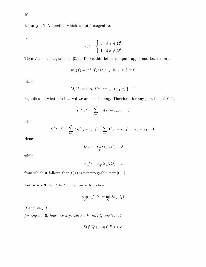
Example 1 A function which is not integrable.

Let

f(x) =

0 if x ∈ Q1

1 if x �∈ Q1

Then f is not integrable on [0,1]! To see this, let us compute upper and lower sums:

mi(f) = inf{f(x) : x ∈ [xi−1, xi]} ≡ 0

while

Mi(f) = sup{f(x) : x ∈ [xi−1, xi]} ≡ 1

regardless of what sub-interval we are considering. Therefore, for any partition of [0, 1],

s(f, P ) =n∑i=1

mi(xi − xi−1) = 0

while

S(f, P ) =n∑i=1

Mi(xi − xi−1) =n∑i=1

1(xi − xi−1) = xn − x0 = 1.

Hence

L(f) = supPs(f, P ) = 0

while

U(f) = infQS(f,Q) = 1

from which it follows that f(x) is not integrable over [0, 1].

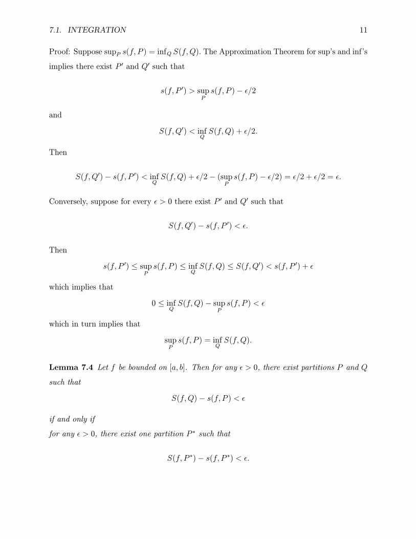
Lemma 7.3 Let f be bounded on [a, b]. Then

supPs(f, P ) = inf

QS(f,Q)

if and only if

for any ε > 0, there exist partitions P ′ and Q′ such that

S(f,Q′)− s(f, P ′) < ε.

7.1. INTEGRATION 11

Proof: Suppose supP s(f, P ) = infQ S(f,Q). The Approximation Theorem for sup’s and inf’s

implies there exist P ′ and Q′ such that

s(f, P ′) > supPs(f, P )− ε/2

and

S(f,Q′) < infQS(f,Q) + ε/2.

Then

S(f,Q′)− s(f, P ′) < infQS(f,Q) + ε/2− (sup

Ps(f, P )− ε/2) = ε/2 + ε/2 = ε.

Conversely, suppose for every ε > 0 there exist P ′ and Q′ such that

S(f,Q′)− s(f, P ′) < ε.

Then

s(f, P ′) ≤ supPs(f, P ) ≤ inf

QS(f,Q) ≤ S(f,Q′) < s(f, P ′) + ε

which implies that

0 ≤ infQS(f,Q)− sup

Ps(f, P ) < ε

which in turn implies that

supPs(f, P ) = inf

QS(f,Q).

Lemma 7.4 Let f be bounded on [a, b]. Then for any ε > 0, there exist partitions P and Q

such that

S(f,Q)− s(f, P ) < ε

if and only if

for any ε > 0, there exist one partition P ∗ such that

S(f, P ∗)− s(f, P ∗) < ε.

12

Proof: Let ε > 0. Suppose there exist partitions P and Q such that

S(f,Q)− s(f, P ) < ε.

By Lemma 7.1,

s(f, P ) ≤ s(f, P ∪Q) ≤ S(f, P ∪Q) ≤ S(f,Q)

which then implies

S(f, P ∪Q)− s(f, P ∪Q) < ε.

Letting P ∗ = P ′ ∪ Q′ then proves the result in one direction. The reverse implication is

trivial, because the existence of P ∗ implies the existence of P and Q, namely, choose P = P ∗

and Q = P ∗.

Combining Lemmas 7.3 and 7.4, we have proved

Theorem 7.5 Let f be bounded on [a, b]. Then f is integrable on [a, b] if and only if for

every ε > 0 there exists a partition P such that

S(f, P )− s(f, P ) < ε.

Theorem 7.6 If f is continuous on [a, b], then f is integrable on [a, b]. I.e. “continuous

functions on closed, bounded intervals are integrable”.

Proof: In light of the preceding theorem, it suffices to prove that for any ε > 0 there is a

partition P such that

S(f, P )− s(f, P ) < ε.

Recall from the Uniform Continuity Theorem, that a continuous function on a closed,

bounded interval is uniformly continuous. Then for any ε > 0 there exists a δ > 0 such that

for all x, y ∈ [a, b],

|x− y| < δ =⇒ |f(x)− f(y)| < ε/(b− a).

If we now choose a partition P of [a, b] which divides [a, b] into n equal size sub-intervals,

each of length (b− a)/n,

P = {x0 < x1 < . . . < xn}

7.1. INTEGRATION 13

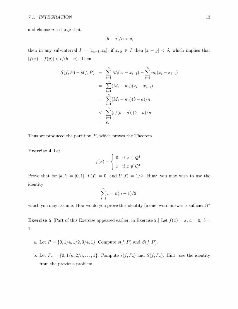
and choose n so large that

(b− a)/n < δ,

then in any sub-interval I = [xk−1, xk], if x, y ∈ I then |x − y| < δ, which implies that

|f(x)− f(y)| < ε/(b− a). Then

S(f, P )− s(f, P ) =n∑i=1

Mi(xi − xi−1)−n∑i=1

mi(xi − xi−1)

=n∑i=1

(Mi −mi)(xi − xi−1)

=n∑i=1

(Mi −mi)(b− a)/n

<n∑i=1

(ε/(b− a))(b− a)/n

= ε.

Thus we produced the partition P , which proves the Theorem.

Exercise 4 Let

f(x) =

0 if x ∈ Q1

x if x �∈ Q1

Prove that for [a, b] = [0, 1], L(f) = 0, and U(f) = 1/2. Hint: you may wish to use the

identityn∑i=1

i = n(n+ 1)/2,

which you may assume. How would you prove this identity (a one- word answer is sufficient)?

Exercise 5 [Part of this Exercise appeared earlier, in Exercise 2.] Let f(x) = x, a = 0, b =

1.

a. Let P = {0, 1/4, 1/2, 3/4, 1}. Compute s(f, P ) and S(f, P ).

b. Let Pn = {0, 1/n, 2/n, . . . , 1}. Compute s(f, Pn) and S(f, Pn). Hint: use the identity

from the previous problem.

14

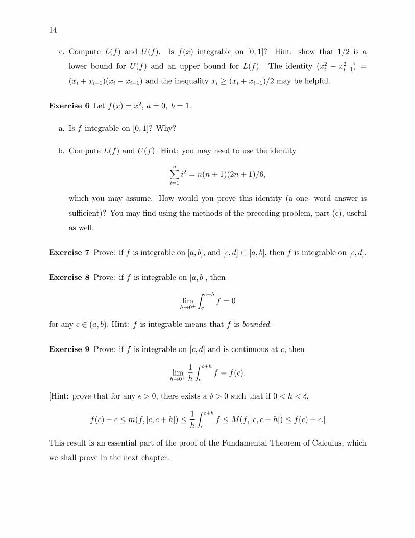
c. Compute L(f) and U(f). Is f(x) integrable on [0, 1]? Hint: show that 1/2 is a

lower bound for U(f) and an upper bound for L(f). The identity (x2i − x2i−1) =

(xi + xi−1)(xi − xi−1) and the inequality xi ≥ (xi + xi−1)/2 may be helpful.

Exercise 6 Let f(x) = x2, a = 0, b = 1.

a. Is f integrable on [0, 1]? Why?

b. Compute L(f) and U(f). Hint: you may need to use the identity

n∑i=1

i2 = n(n+ 1)(2n+ 1)/6,

which you may assume. How would you prove this identity (a one- word answer is

sufficient)? You may find using the methods of the preceding problem, part (c), useful

as well.

Exercise 7 Prove: if f is integrable on [a, b], and [c, d] ⊂ [a, b], then f is integrable on [c, d].

Exercise 8 Prove: if f is integrable on [a, b], then

limh→0+

∫ c+hcf = 0

for any c ∈ (a, b). Hint: f is integrable means that f is bounded.

Exercise 9 Prove: if f is integrable on [c, d] and is continuous at c, then

limh→0+

1

h

∫ c+hcf = f(c).

[Hint: prove that for any ε > 0, there exists a δ > 0 such that if 0 < h < δ,

f(c)− ε ≤ m(f, [c, c+ h]) ≤1

h

∫ c+hcf ≤ M(f, [c, c+ h]) ≤ f(c) + ε.]

This result is an essential part of the proof of the Fundamental Theorem of Calculus, which

we shall prove in the next chapter.

7.1. INTEGRATION 15

The Riemann Integral

What we have introduced so far is the Darboux integral. The Riemann integral is equivalent

to the Darboux integral, in that for any function f , the Darboux Integral of f exists if and

only if the Riemann Integral of f exists, and the two integrals are equal. We shall not prove

this here. What we prove is that under the assumption that the function f is continuous,

the Riemann integral exists, and its value is the same as that of the Darboux integral.

Definition 7.4 Suppose f(x) is a function defined on [a, b], with the following properties:

Suppose P = {x0, x1, . . . , xn} is a partition of the interval [a, b], and x∗i is chosen in any

fashion from the i-th subinterval: x∗i ∈ [xi−1, xi]. Let ||P || denote the length of the largest

subinterval [xi−1, xi], 1 ≤ i ≤ n. We say that “f is Riemann integrable on the interval

[a, b]” and “the Riemann integral of f over [a, b] is I” if I is a real number such that for

every ε > 0 there exists a δ > 0 such that if P = {x0, x1, . . . , xn} is any partition of [a, b]

and ||P || < δ, then |∑ni=1 f(x

∗i )(xi − xi−1)− I| < ε, or what is the same,

lim||P ||→0

n∑i=1

f(x∗i )(xi − xi−1) = I.

Comments: a few remarks about the Riemann integral. What makes the definition a bit

unwieldy is the large number of quantifiers. Recall that as soon as we speak about it limits,

we are making an ε − δ statement. Then we have the partitions, then the choice of x∗i ’s in

the i-th sub-interval. It’s all quite messy. That is why we are restricting our attention to

this special case.

Theorem 7.7 Suppose f(x) is continuous on [a, b]. Then the Riemann integral of f over

[a, b] exists, and equals L(f).

Proof: We already know from Theorem 7.6 that for continuous functions, L(f) = U(f). Let

I = U(f) = L(f). To prove

lim||P ||→0

n∑i=1

f(x∗i )(xi − xi−1) = I,

16

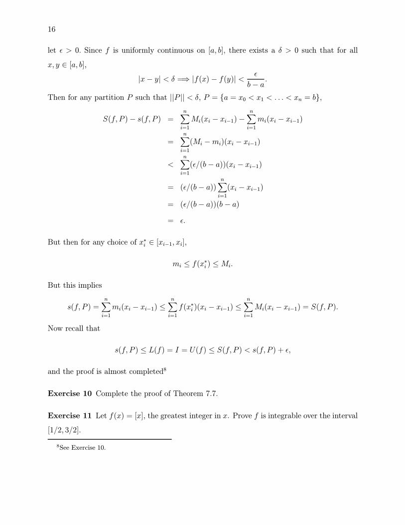
let ε > 0. Since f is uniformly continuous on [a, b], there exists a δ > 0 such that for all

x, y ∈ [a, b],

|x− y| < δ =⇒ |f(x)− f(y)| <ε

b− a.

Then for any partition P such that ||P || < δ, P = {a = x0 < x1 < . . . < xn = b},

S(f, P )− s(f, P ) =n∑i=1

Mi(xi − xi−1)−n∑i=1

mi(xi − xi−1)

=n∑i=1

(Mi −mi)(xi − xi−1)

<n∑i=1

(ε/(b− a))(xi − xi−1)

= (ε/(b− a))n∑i=1

(xi − xi−1)

= (ε/(b− a))(b− a)

= ε.

But then for any choice of x∗i ∈ [xi−1, xi],

mi ≤ f(x∗i ) ≤ Mi.

But this implies

s(f, P ) =n∑i=1

mi(xi − xi−1) ≤n∑i=1

f(x∗i )(xi − xi−1) ≤n∑i=1

Mi(xi − xi−1) = S(f, P ).

Now recall that

s(f, P ) ≤ L(f) = I = U(f) ≤ S(f, P ) < s(f, P ) + ε,

and the proof is almost completed8

Exercise 10 Complete the proof of Theorem 7.7.

Exercise 11 Let f(x) = [x], the greatest integer in x. Prove f is integrable over the interval

[1/2, 3/2].

8See Exercise 10.

7.1. INTEGRATION 17

Properties of the Darboux Integral

We now develop the properties of the (Darboux) integral, namely that the integral is a

positive, linear functional:

Definition 7.5 A function L whose domain is a set of functions, and whose range is R1 is

called a linear functional if

L(f + g) = L(f) + L(g)

and

L(cf) = cL(f)

for all functions f and g, and all constants c. A linear functional with the further property

that

L(f) ≥ 0

for any f such that f(x) ≥ 0 will be called a positive linear functional

Theorem 7.8 (The Darboux Integral is a positive linear functional.) If f and g are

both integrable on the interval [a, b], then so are f + g and cf , for any real number c. When

f and g are both integrable, ∫ ba(f + g) =

∫ baf +

∫ bag

and ∫ bacf = c

∫ baf.

If f(x) ≥ 0 for all x ∈ [a, b], then ∫ baf ≥ 0.

First, we prove a lemma, which we shall need in the course of the proof of the theorem:

Lemma 7.9 If f is integrable on [a, b], then −f is integrable on [a, b], and

∫ ba(−f) = −

∫ baf.

18

Proof: Since f is integrable, let ε > 0 and P a partition of [a, b] for which

S(f, P )− s(f, P ) < ε.

Then

S(−f, P )− s(−f, P ) = −s(f, P ) + S(f, P ) < ε,

which shows −f is integrable on P . Then∫ ba (−f) = U(−f) = infP S(−f, P ) =

9 infP{−s(f, P )} =

− supP s(f, P ) = −L(f) = −∫ ba f.

Proof of the Theorem: We prove this in several parts:

1. If f and g are integrable on [a, b] then so is f + g.

2. In this case ∫ baf + g =

∫ baf +

∫ bag.

3. If f is integrable,∫ ba cf = c

∫ ba f.

4. The (Darboux) Integral is a positive functional.

To prove (1), suppose ε > 0. Theorem 7.5 implies (after a little work) there exists a

partition P such that10 both

S(f, P )− s(f, P ) < ε/2

and

S(g, P )− s(g, P ) < ε/2.

Then

S(f + g, P ) =n∑i=1

Mi(f + g)(xi − xi−1) ≤n∑i=1

Mi(f)(xi − xi−1) +n∑i=1

Mi(g)(xi − xi−1)

= S(f, P ) + S(g, P )

9Why?

10See Exercise 12. You need to construct this partition.

7.1. INTEGRATION 19

and

s(f + g, P ) =n∑i=1

mi(f + g)(xi − xi−1) ≥n∑i=1

mi(f)(xi − xi−1) +n∑i=1

mi(g)(xi − xi−1)

= s(f, P ) + s(g, P )

But then

S(f + g, P )− s(f + g, P ) ≤ S(f, P ) + S(g, P )− (s(f, P ) + s(g, P ))

= S(f, P )− s(f, P ) + S(g, P )− s(g, P ) < ε/2 + ε/2 = ε,

which, by Theorem 7.5, proves that f + g is integrable on [a, b]. To prove (2) we evaluate

U(f + g). Consider the following (for the partition P we used above):

L(f + g) = U(f + g) ≤ S(f + g, P ) ≤ S(f, P ) + S(g, P )

≤ s(f, P ) + s(g, P ) + ε

≤ L(f) + L(g) + ε.

In a similar11 way,

U(f + g) ≥ U(f) + U(g)− ε.

Combining these two results, we obtain

U(f) + U(g)− ε ≤ L(f + g) = U(f + g) ≤ L(f) + L(g) + ε = U(f) + U(g) + ε.

Thus U(f + g) = U(f) + U(g).

To prove (3), if c > 0, then

U(cf) = infPS(cf, P ) = inf

PcS(f, P ) = c inf

PS(f, P ) = cU(f).

If c < 0, then

∫ bacf =

∫ ba(−c)(−f) = −c

∫ ba(−f) = (−c)(−

∫ baf) = c

∫ baf.

11Provide the reasoning.

20

Finally, to prove (4), assume f(x) ≥ 0 and f integrable. For any partition ||P ||,Mi(f) ≥ 0

since f(x) ≥ 0. Therefore S(f, P ) ≥ 0, and hence (why?) infP S(f, P ) ≥ 0. Then U(f) ≥ 0.

But since f is integrable, ∫ baf = U(f) ≥ 0.

Corollary 7.10 If f and g are integrable on [a, b], and f(x) ≤ g(x), for all x ∈ [a, b], then

∫ baf ≤

∫ bag.

Proof: By Theorem 7.8, g − f is integrable, and g − f ≥ 0. So∫ ba g −

∫ ba f =

∫ ba (g − f) ≥ 0.

Exercise 12 Prove that if f and g are integrable on [a, b], then for every ε > 0 there exists

a partition P such that S(f, P )− s(f, P ) < ε/2 and S(g, P )− s(g, P ) < ε/2.

Exercise 13 Suppose we consider only those functions which are differentiable at 0. Us-

ing your basic knowledge from introductory calculus, verify that differentiation and then

evaluation at 0 is a positive linear functional (that is, the function Φ defined by

Φ(f) = f ′(0) for every differentiable f

is a positive linear functional.)

Theorem 7.11 (Triangle Inequality for Integrals) If f is integrable on [a, b], then

|∫ baf | ≤

∫ ba|f |.

Proof: Recall that for any real numbers a and b,

|a| = |a− b+ b| ≤ |a− b| + |b|

from which it follows that

|a| − |b| ≤ |a− b|.

Therefore12, for any partition P of [a, b],

Mi(|f |)−mi(|f |) ≤Mi(f)−mi(f) (7.2)

12Provide the details. See Exercise 14.

7.1. INTEGRATION 21

from which it follows that

S(|f |, P )− s(|f |, P ) ≤ S(f, P )− s(f, P ).

Since we assumed f was integrable, for any ε > 0 there is a partition P such that S(f, P )−

s(f, P ) < ε. It then follows that S(|f |, P )− s(|f |, P ) < ε, which shows |f | is integrable.

Now recall that for any x,

−|f(x)| ≤ f(x) ≤ |f(x)|

so by Corollary 7.10,

−∫ ba|f | ≤

∫ baf ≤

∫ ba|f |,

i.e.,

|∫ baf | ≤

∫ ba|f |.

Exercise 14 Prove Equation 7.2.

Definition 7.6 A function f is said to be piecewise continuous on the interval [a, b] if

there exists a partition P = {x0, x1, . . . , xn} of [a, b] such that f(x) is continuous on the open

subintervals (xi−1, xi), 1 ≤ i ≤ n.

Note: informally, a piecewise continuous function is one which is continuous, except at a

finite number of discontinuities (which, in our definition above, are x1, . . . , xn−1.)

Example 2 f(x) = [x] restricted to the interval [0, 10] has discontinuities at {1, 2, . . . , 10}.

Theorem 7.12 A bounded, piecewise continuous function on [a, b] is integrable on [a, b].

Proof: First we need a helpful Lemma:

Lemma 7.13 If f is continuous and bounded on the open interval (a, b) then f is integrable

on [a, b].

22

Proof of the Lemma:

Let ε > 0. Suppose |f(x)| ≤M on (a, b). Choose δ = min{ε/8M, (b−a)/2)}13. f is continuous

on [a+ δ, b− δ], so f is uniformly continuous there, hence integrable on [a+ δ, b− δ]. Hence

there exists a partition P of [a + δ, b− δ] such that

S(f, P )− s(f, P ) < ε/2.

Now,

P ∗ = P ∪ {a, b}

is a partition of [a, b], and

S(f, P ∗)− s(f, P ∗) = S(f, P )− s(f, P ) + 2M(a + δ − a) + 2M(b− (b− δ))

<ε

2+ 2M(2δ)

≤ ε.

Hence f is integrable on (a, b) by Theorem 7.5.

Proof of Theorem 7.12: Suppose f is bounded on (a, b) and continuous on (a, b) except

perhaps at the points {x1, . . . , xn}. Then by Lemma 7.13 f is integrable on each subinterval

(x0, x1), (x1, x2), . . . , (xn−1, xn). Let ε > 0 and choose partitions Pi on (xi−1, xi) such that

S(f, Pi) − s(f, Pi) < ε/n. Then let P = P1 ∪ . . . Pn, and P is then a partition of (a, b) for

which S(f, P )− s(f, P ) < ε. Hence f is integrable on (a, b).

Definition: A function f(x) is said to be monotonic on the interval I if x < y =⇒

f(x) ≤ f(y) for all x, y ∈ I.

Theorem 7.14 A monotonic function f defined on [a, b] is integrable on [a, b].

Proof: Assume that f is monotone increasing. Let ε > 0. Let δ = ε/(f(b)− f(a)). Then let

P = {x0, x1, . . . , xn} be any partition for which ||P || < δ. For this partition,

S(f, P ) =n∑i=1

Mi(f)(xi − xi−1)

=n∑i=1

f(xi)(xi − xi−1)

13Why must δ ≤ (b− a)/2?

7.1. INTEGRATION 23

while

s(f, P ) =n∑i=1

mi(f)(xi − xi−1)

=n∑i=1

f(xi−1)(xi − xi−1)

so that

S(f, P )− s(f, P ) =n∑i=1

(f(xi)− f(xi−1))(xi − xi−1)

≤n∑i=1

(f(xi)− f(xi−1))δ

≤ δn∑i=1

(f(xi)− f(xi−1))

≤ δ(f(xn)− f(x0))

= ε/(f(b)− f(a)) · (f(b)− f(a))

= ε.

Thus, by Theorem 7.5, f is integrable on [a, b]. If f is monotone decreasing, consider −f

instead.

Theorem 7.15 If f is integrable on [a, b], and also on [b, c], then f is integrable on [a, c]

and ∫ caf =

∫ baf +

∫ cbf.

Proof: See Exercise 15.

Exercise 15 Prove Theorem 7.15.

Definition 7.7 We shall also need to be able to compute the value of∫ ba f in the case where

b < a, and for this reason we define

∫ baf = −

∫ abf if a < b.

24

Theorem 7.16 (Mean Value Theorem for Integrals) Suppose f is continuous on [a, b].

Then there exists a c, a < c < b such that

f(c) =1

b− a

∫ baf.

Proof: Since f is continuous, m = inf [a,b] f(x) andM = sup[a,b] f(x) both exist, and therefore∫ bam ≤

∫ baf ≤

∫ baM,

from which it follows (why?) that

m ≤1

b− a

∫ baf ≤M.

But f(x) takes the values m and M , by the Extreme Value Theorem, and therefore14 there

is a c ∈ [a, b] such that

f(c) =1

b− a

∫ baf.

Exercise 16 Give an example of a function f(x) ≥ 0, f(x) �≡ 0 on the interval [0, 1] which

is integrable, but for which U(f) = L(f) = 0. Hint: this function cannot be continuous on

[0, 1].

Exercise 17 Prove: Suppose f(x) is continuous on [0, 1] and f(x) ≥ 0. If f(x0) > 0 for

some x0 ∈ [0, 1], then∫ 10 f > 0.

Exercise 18 Prove that if f(x) is integrable on [a, b] and g(x) = f(x), except at a finite

number of points, x1, . . . , xn ∈ [a, b], then g(x) is integrable on [a, b] and∫ bag =

∫ baf.

7.1.2 Improper Integrals

We can extend our abilities to integrate functions in two different ways: First, we can,

under certain circumstances, allow either or both of the limits of integration to be infinite.

Second, we can allow the function f to be unbounded, in some circumstances. We shall deal

separately with these two issues:

14Why? Quote the appropriate theorem to justify this.

7.1. INTEGRATION 25

Improper integrals of type∫∞a f or

∫∞−∞ f.

If we wish to compute the integral of some function f , say over [0,∞) there is no convenient

way to speak about this integral in terms of upper and lower sums, or Riemann sums, for

that matter. The problem is that the interval over which we are integrating is infinite. The

way out of this difficulty is to consider the integral

∫ M0f(x)dx

as an approximation to ∫ ∞0f(x)dx

when M is large. More precisely, we shall define the latter as the limit of the former:

Definition 7.8 Suppose f(x) is defined on (at least) the interval [a,∞), for some real num-

ber a. Then we define ∫ ∞af(x)dx

as the limit

limM→∞

∫ Maf(x)dx.

If this limit does not exist, we say the integral does not exist. When the limit does exist,

we call this the improper Riemann integral of f , and we say the integral converges.

If the limit exists but equals +∞, we say the integral diverges to +∞.

Example 3∫∞1 1/x

2dx. To see if this integral converges, we compute

∫ ∞1

1

x2dx = lim

M→∞

∫ M1

1

x2dx

= limM→∞

(−1

x)]M1

= limM→∞

1−1

M

= 1.

26

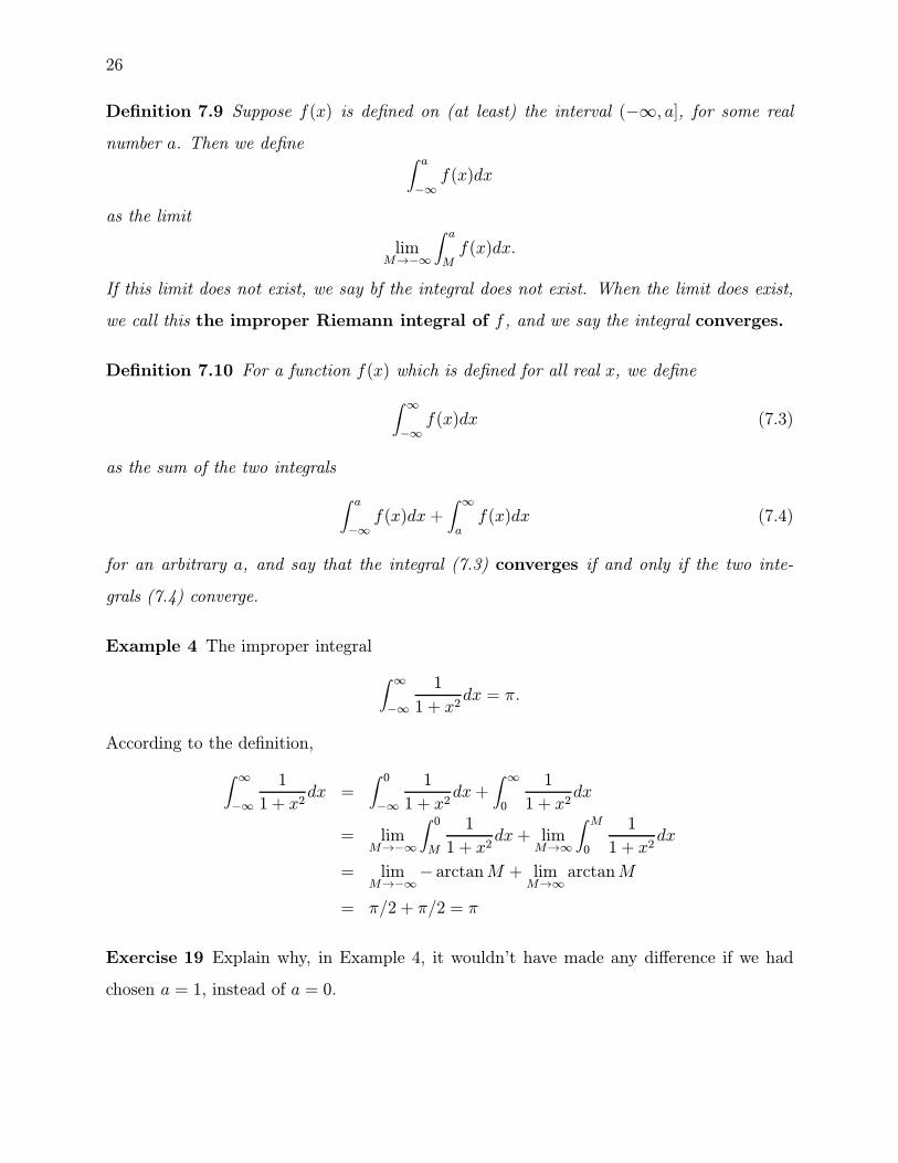
Definition 7.9 Suppose f(x) is defined on (at least) the interval (−∞, a], for some real

number a. Then we define ∫ a−∞f(x)dx

as the limit

limM→−∞

∫ aMf(x)dx.

If this limit does not exist, we say bf the integral does not exist. When the limit does exist,

we call this the improper Riemann integral of f , and we say the integral converges.

Definition 7.10 For a function f(x) which is defined for all real x, we define

∫ ∞−∞f(x)dx (7.3)

as the sum of the two integrals

∫ a−∞f(x)dx+

∫ ∞af(x)dx (7.4)

for an arbitrary a, and say that the integral (7.3) converges if and only if the two inte-

grals (7.4) converge.

Example 4 The improper integral

∫ ∞−∞

1

1 + x2dx = π.

According to the definition,

∫ ∞−∞

1

1 + x2dx =

∫ 0−∞

1

1 + x2dx+

∫ ∞0

1

1 + x2dx

= limM→−∞

∫ 0M

1

1 + x2dx+ lim

M→∞

∫ M0

1

1 + x2dx

= limM→−∞

− arctanM + limM→∞

arctanM

= π/2 + π/2 = π

Exercise 19 Explain why, in Example 4, it wouldn’t have made any difference if we had

chosen a = 1, instead of a = 0.

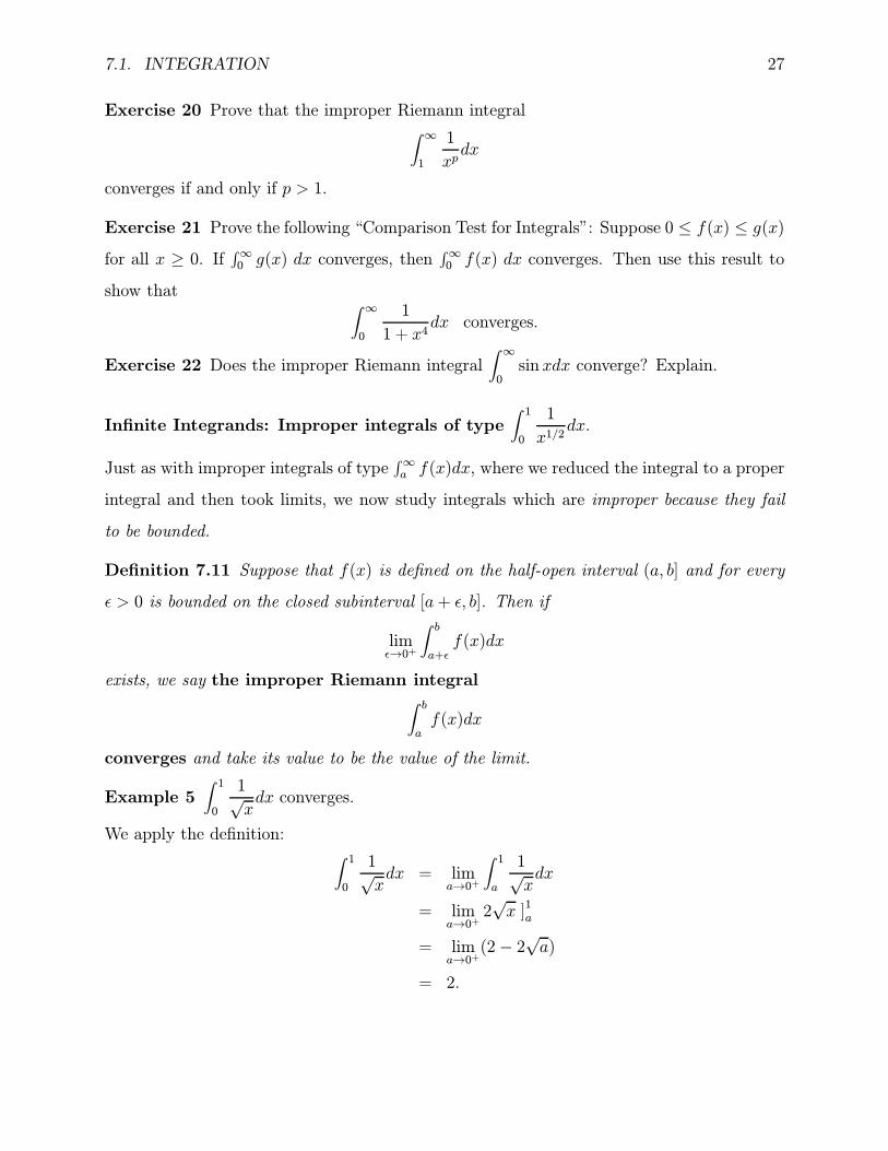
7.1. INTEGRATION 27

Exercise 20 Prove that the improper Riemann integral∫ ∞1

1

xpdx

converges if and only if p > 1.

Exercise 21 Prove the following “Comparison Test for Integrals”: Suppose 0 ≤ f(x) ≤ g(x)

for all x ≥ 0. If∫∞0 g(x) dx converges, then

∫∞0 f(x) dx converges. Then use this result to

show that ∫ ∞0

1

1 + x4dx converges.

Exercise 22 Does the improper Riemann integral∫ ∞0sin xdx converge? Explain.

Infinite Integrands: Improper integrals of type∫ 10

1

x1/2dx.

Just as with improper integrals of type∫∞a f(x)dx, where we reduced the integral to a proper

integral and then took limits, we now study integrals which are improper because they fail

to be bounded.

Definition 7.11 Suppose that f(x) is defined on the half-open interval (a, b] and for every

ε > 0 is bounded on the closed subinterval [a+ ε, b]. Then if

limε→0+

∫ ba+εf(x)dx

exists, we say the improper Riemann integral∫ baf(x)dx

converges and take its value to be the value of the limit.

Example 5∫ 10

1√xdx converges.

We apply the definition:∫ 10

1√xdx = lim

a→0+

∫ 1a

1√xdx

= lima→0+

2√x ]1a

= lima→0+(2− 2

√a)

= 2.

28

Exercise 23 Prove that the improper Riemann integral

∫ 10

1

xpdx

converges if and only if p < 1.

If f(x) is unbounded at b rather than at a, the definition is similar:

Definition 7.12 Suppose that f(x) is defined on the half-open interval [a, b) and for every

ε > 0 is bounded on the closed subinterval [a, b− ε]. Then if

limε→0+

∫ b−εaf(x)dx

exists, we say the improper Riemann integral

∫ baf(x)dx

converges and take its value to be the value of the limit.