7 Applicably and Validity of the Proposed Alternative Methodology 149

7Applicably and Validity of the Proposed AlternativeMethodology

7.1.Introduction

This Chapter presents the evaluation and validation of the alternative

methodology developed in Chapter 6 for extending the range of application of

available data so as to produce moment-rotation characteristics that implicitly

make proper allowance for the presence of significant levels of either tension or

compression in the beam. This assessment is executed against a range of available

experimental tests for flush endplate joints (Simões da Silva et al., 2004) and

baseplate joints (Guisse et al., 1996).

7.2.Application of the Alternative Methodology

The main focus of the methodology presented in Chapter 6 is to determine

M- curves for any axial force level from two reference M- curves. The quality

of the obtained approximations depends on the quality of the M- curves used as

input to the method.

This methodology requires, at least, two M- curves, disregarding and

considering either the compressive or tensile axial force effect. However, for a

complete behavioural evaluation of the joint three M- curves are necessary: one

disregarding the axial force effect; another considering the compressive force

effect and finally a third alternative considering the tensile force effect. In this

way, it is possible to study the entirely joint structural response given that loading

applied to the joint may vary from compression to tension.

In order to explain the application of this method to obtain M- curves for

any axial force level, as well as to validate its use, experimental tests carried out

by Lima (2003) and Simões da Silva et al. (2004), and Guisse et al. (1996), on

eight flush endplate joints and twelve column bases have been used.

7 Applicably and Validity of the Proposed Alternative Methodology 150

7.2.1.Flush endplate joints

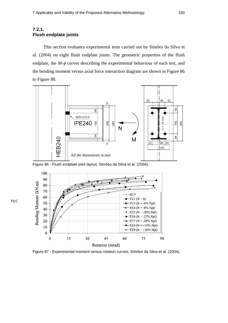
This section evaluates experimental tests carried out by Simões da Silva et

al. (2004) on eight flush endplate joints. The geometric properties of the flush

endplate, the M- curves describing the experimental behaviour of each test, and

the bending moment versus axial force interaction diagram are shown in Figure 86

to Figure 88.

Figure 86 - Flush endplate joint layout, Simões da Silva et al. (2004).

Figure 87 - Experimental moment versus rotation curves, Simões da Silva et al. (2004).

All the dimensions in mm

7 Applicably and Validity of the Proposed Alternative Methodology 151

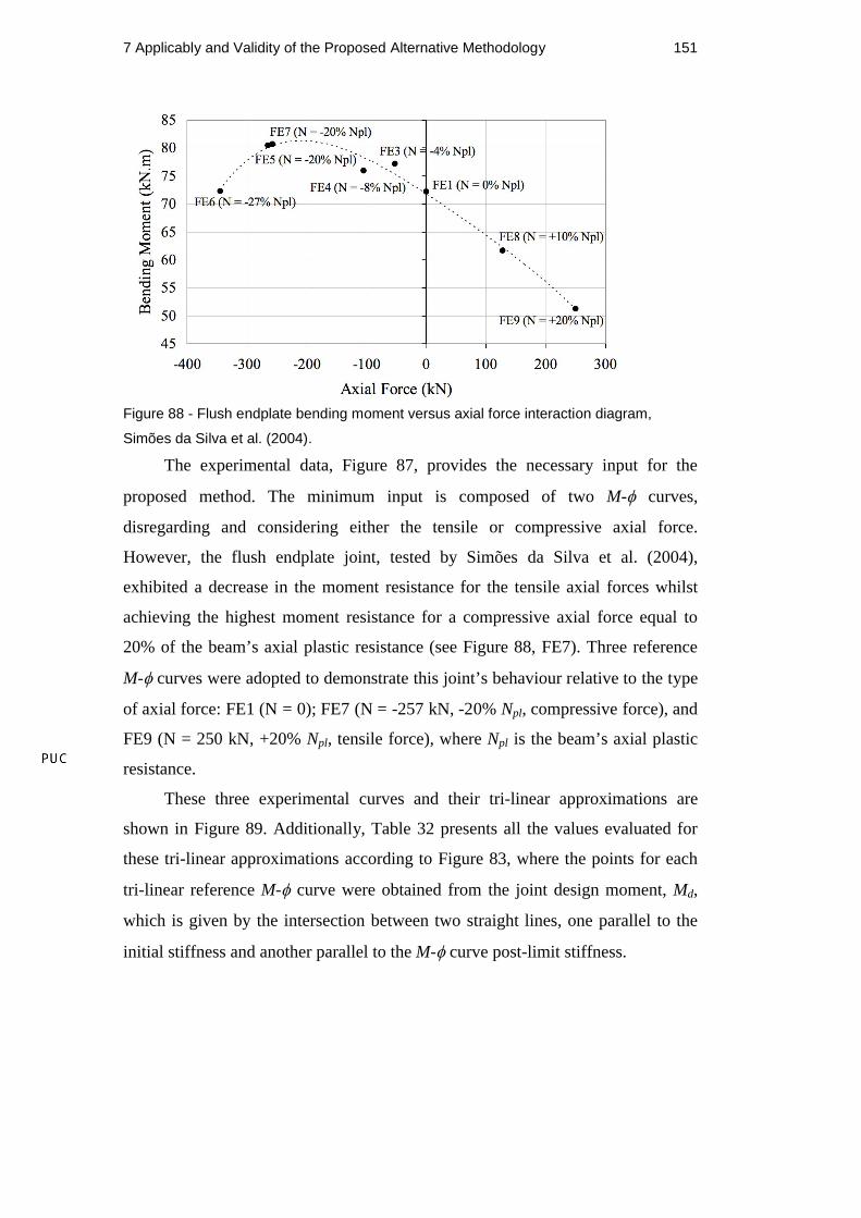
Figure 88 - Flush endplate bending moment versus axial force interaction diagram,

Simões da Silva et al. (2004).

The experimental data, Figure 87, provides the necessary input for the

proposed method. The minimum input is composed of two M- curves,

disregarding and considering either the tensile or compressive axial force.

However, the flush endplate joint, tested by Simões da Silva et al. (2004),

exhibited a decrease in the moment resistance for the tensile axial forces whilst

achieving the highest moment resistance for a compressive axial force equal to

20% of the beam’s axial plastic resistance (see Figure 88, FE7). Three reference

M- curves were adopted to demonstrate this joint’s behaviour relative to the type

of axial force: FE1 (N = 0); FE7 (N = -257 kN, -20% Npl, compressive force), and

FE9 (N = 250 kN, +20% Npl, tensile force), where Npl is the beam’s axial plastic

resistance.

These three experimental curves and their tri-linear approximations are

shown in Figure 89. Additionally, Table 32 presents all the values evaluated for

these tri-linear approximations according to Figure 83, where the points for each

tri-linear reference M- curve were obtained from the joint design moment, Md,

which is given by the intersection between two straight lines, one parallel to the

initial stiffness and another parallel to the M- curve post-limit stiffness.

7 Applicably and Validity of the Proposed Alternative Methodology 152

Table 32 - Values evaluated for the reference M- curves.

FE1(N = 0.0)

FE7(N = -257 kN, -20% Npl)

FE9(N = +250 kN, +20% Npl)

Point (mrad) M (kNm) (mrad) M (kNm) (mrad) M (kNm)

0 0.0 0.0 0.0 0.0 0.0 0.0

2/3 Md 6.3 50.6 6.8 56.1 13.0 38.4

Md 27.6 76.0 26.8 84.1 25.8 57.7

1.1 Md 56.1 83.5 67.3 92.2 35.0 63.5

Tri-linear M- curves, Figure 89, are used to define paths between each

curve at points 2/3Md, Md and 1.1Md, Figure 90. These paths were used to guide

the linear interpolators for bending moments, Eq. (6.4), and rotations, Eq. (6.5),

throughout the given range of axial force levels to determine the required set of

M- curves.

Figure 89 - Tri-linear strategy used for the experimental M- curves.

7 Applicably and Validity of the Proposed Alternative Methodology 153

Figure 90 - Paths used to define the procedure to determine any M- curve present within

these limits.

Subsequently, Table 33 depicts the results obtained by using the proposed

methodology to predict three experimental M- curves: FE8 for a 10% tensile

force of the beam’s axial plastic resistance, FE3 and FE4 for compressive forces

of 4% and 8%, respectively, of the beam’s axial plastic resistance.

Following this strategy, as an example, Eq. (7.1) demonstrates how to

calculate point 1.1Md, Table 33, of the FE8 approximated M- curve. Figure 91 to

Figure 93 graphically depict these results. Figure 94 presents the whole set of

predicted M- curves utilising this methodology.

Table 33 - Values evaluated for three tri-linearly approximated M- curves.

FE3(Ni = -53 kN, -4% Npl)

FE4(Ni = -105 kN, -8% Npl)

FE8(Ni = +128 kN, +10% Npl)

Point (mrad) M (kNm) (mrad) M (kNm) (mrad) M (kNm)

0 0.0 0.0 0.0 0.0 0.0 0.0

2/3 Md 6.4 51.8 6.5 52.9 9.7 44.4

Md 27.4 77.6 27.3 79.3 26.7 66.6

1.1 Md 58.4 85.3 60.7 87.1 45.3 73.3

7 Applicably and Validity of the Proposed Alternative Methodology 154

1:2,0

9:2;,

3.451.560.250

0.1281.560.35

,0,0,

3.735.830.250

0.1285.835.63

,0,0,

,0

,

1.1int:8

FETableandp

M

FETableNandpN

M

mradpN

iN

ppNp

kNmp

MN

iN

pM

pNM

pM

p

pN

dMpPoFE

(7.1)

Figure 91 - FE8 M- curve approximation, considering a tensile force of 10% of the

beam’s axial plastic resistance.

Figure 92 - FE3 M- curve approximation, considering a compressive force of 4% of the

beam’s axial plastic resistance.

7 Applicably and Validity of the Proposed Alternative Methodology 155

Figure 93 - FE4 M- curve approximation, considering a compressive force of 8% of the

beam’s axial plastic resistance.

Figure 94 - The whole set of predicted M- curves by using the proposed methodology.

7.2.2.Column bases

This section presents the evaluation of the experiments performed by Guisse

et al. (1996) on twelve column base joints. Test configurations with respectively

four and two anchor bolts, Figure 95(a) and Figure 95(b), were considered. The

steel column profile was a S355 HE160B, whilst the S235 baseplates utilised two

different thicknesses: 15 mm and 30 mm. The baseplates are welded to the

column with 6 mm fillet welds connected with M20 10.9 anchor bolts.

7 Applicably and Validity of the Proposed Alternative Methodology 156

45 mm

45 mm

250 mm340 mm

220 mm

HE 160B

M 20

110 mm

220 mm

50 mm 50 mm120 mm

220 mm

HE 160B

M 20

110 mm

(a) Four anchor bolts. (b) Two anchor bolts.

Figure 95 - Baseplate configurations, Guisse et al. (1996).

Table 34 presents the set of the tested column bases and Figure 96 to Figure

99 show the experimental M- curves obtained by Guisse et al. (1996).

Table 34 - Nomenclature of the tests and their parameters, Guisse et al. (1996).

Name Anchor bolts Plate thickness (mm) Normal force (kN)PC2.15.100 2 15 100PC2.15.600 2 15 600PC2.15.1000 2 15 1000PC2.30.100 2 30 100PC2.30.600 2 30 600PC2.30.1000 2 30 1000PC4.15.100 4 15 100PC4.15.400 4 15 400PC4.15.1000 4 15 1000PC4.30.100 4 30 100PC4.30.400 4 30 400PC4.30.1000 4 30 1000

Since the experiments used only compressive forces, two reference M-

curves were adopted for each set of tests related to the axial forces of 100 and

1000 kN. The experimental M- curves and their tri-linear approximations are

shown in Figure 96 to Figure 99. Additionally, Table 35 presents all the values

evaluated for these tri-linear approximations according to Figure 83.

7 Applicably and Validity of the Proposed Alternative Methodology 157

Table 35 - Values evaluated for the reference M- curves.P

oin

t PC2 PC415.100 15.1000 30.100 30.1000 15.100 15.1000 30.100 30.1000 M M M M M M M M

0 0 0 0 0 0 0 0 0 0 0 0 0 0 0 0 02/3Md 21 21 9 41 25 17 11 46 10 32 16 63 12 46 11 72

Md 40 32 30 62 44 26 29 69 28 48 40 94 33 69 35 1081.1Md 50 35 60 62 51 29 62 75 43 53 60 94 50 76 64 108

Note: M in kNm and in mrad.

0

10

20

30

40

50

60

70

80

0 15 30 45 60 75 90

Rotation (mrad)

Ben

ding

Mom

ent (

kN.m

)

PC2.15.100: experimentalPC2.15.600: experimentalPC2.15.1000: experimentalPC2.15.100: tri-linearPC2.15.1000: tri-linear

upper compressive limit (N = -1000 kN)

lower compressive limit (N = -100 kN)

Figure 96 - PC2.15 experimental M- curves and the tri-linear reference M- curves.

0

10

20

30

40

50

60

70

80

0 15 30 45 60 75 90

Rotation (mrad)

Ben

ding

Mom

ent (

kN.m

)

PC2.30.100: experimentalPC2.30.600: experimentalPC2.30.1000: experimentalPC2.30.100: tri-linearPC2.30.1000: tri-linear

upper compressive limit (N = -1000 kN)

lower compressive limit (N = -100 kN)

Figure 97 - PC2.30 experimental M- curves and the tri-linear reference M- curves.

7 Applicably and Validity of the Proposed Alternative Methodology 158

0

20

40

60

80

100

120

0 15 30 45 60 75 90

Rotation (mrad)

Ben

ding

Mom

ent (

kN.m

)

PC4.15.100: experimentalPC4.15.400: experimentalPC4.15.1000: experimentalPC4.15.100: tri-linearPC4.15.1000: tri-linear

upper compressive limit (N = -1000 kN)

lower compressive limit (N = -100 kN)

Figure 98 - PC4.15 experimental M- curves and the tri-linear reference M- curves.

0

20

40

60

80

100

120

0 15 30 45 60 75 90

Rotation (mrad)

Ben

ding

Mom

ent (

kN.m

)

PC4.30.100: experimentalPC4.30.400: experimentalPC4.30.1000: experimentalPC4.30.100: tri-linearPC4.30.1000: tri-linear

upper compressive limit (N = -1000 kN)

lower compressive limit (N = -100 kN)

Figure 99 - PC4.30 experimental M- curves and the tri-linear reference M- curves.

Table 36 presents the results obtained by using the proposed method, with

the aid of Eqs. (6.4) and (6.5), to predict four experimental M- curves:

PC2.15.600; PC2.30.600; PC4.15.400 and PC4.30.400.

Table 36 - Values evaluated for three tri-linearly approximated M- curves.

Poi

nt PC2 PC4

15.600 30.600 15.400 30.400 M M M M

0 0.0 0.0 0.0 0.0 0.0 0.0 0.0 0.02/3Md 13.0 34.7 15.3 36.4 12.7 45.6 11.6 57.6

Md 33.3 52.0 34.0 54.7 33.3 68.4 33.9 86.31.1Md 56.7 53.1 58.3 60.1 50.6 71.1 56.2 90.2

Note: M in kNm and in mrad. Ni is equal to 600 kN for PC2 and 400 kN for PC4.

7 Applicably and Validity of the Proposed Alternative Methodology 159

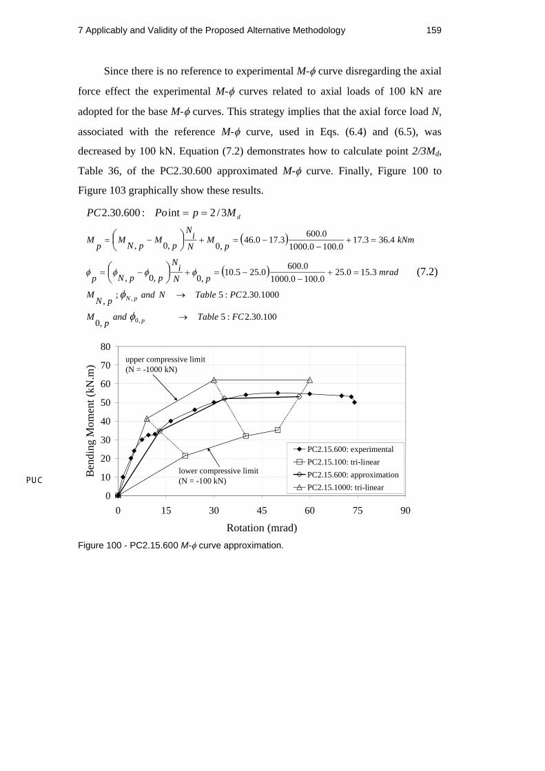
Since there is no reference to experimental M- curve disregarding the axial

force effect the experimental M- curves related to axial loads of 100 kN are

adopted for the base M- curves. This strategy implies that the axial force load N,

associated with the reference M- curve, used in Eqs. (6.4) and (6.5), was

decreased by 100 kN. Equation (7.2) demonstrates how to calculate point 2/3Md,

Table 36, of the PC2.30.600 approximated M- curve. Finally, Figure 100 to

Figure 103 graphically show these results.

100.30.2:5,0

1000.30.2:5;,

3.150.250.1000.1000

0.6000.255.10

,0,0,

4.363.170.1000.1000

0.6003.170.46

,0,0,

,0

,

3/2int:600.30.2

FCTableandp

M

PCTableNandpN

M

mradpN

iN

ppNp

kNmp

MN

iN

pM

pNM

pM

p

pN

dMpPoPC

(7.2)

0

10

20

30

40

50

60

70

80

0 15 30 45 60 75 90

Rotation (mrad)

Ben

ding

Mom

ent (

kN.m

)

PC2.15.600: experimental

PC2.15.100: tri-linear

PC2.15.600: approximation

PC2.15.1000: tri-linear

upper compressive limit (N = -1000 kN)

lower compressive limit (N = -100 kN)

Figure 100 - PC2.15.600 M- curve approximation.

7 Applicably and Validity of the Proposed Alternative Methodology 160

0

10

20

30

40

50

60

70

80

0 15 30 45 60 75 90

Rotation (mrad)

Ben

ding

Mom

ent (

kN.m

)

PC2.30.600: experimental

PC2.30.100: tri-linear

PC2.30.600: approximation

PC2.30.1000: tri-linear

upper compressive limit (N = -1000 kN)

lower compressive limit (N = -100 kN)

Figure 101 - PC2.30.600 M- curve approximation.

0

20

40

60

80

100

120

0 15 30 45 60 75 90

Rotation (mrad)

Ben

ding

Mom

ent (

kN.m

)

PC4.15.400: experimental

PC4.15.100: tri-linear

PC4.15.400: approximation

PC4.15.1000: tri-linear

upper compressive limit (N = -1000 kN)

lower compressive limit (N = -100 kN)

Figure 102 - PC4.15.400 M- curve approximation.

7 Applicably and Validity of the Proposed Alternative Methodology 161

0

20

40

60

80

100

120

0 15 30 45 60 75 90

Rotation (mrad)

Ben

ding

Mom

ent (

kN.m

)

PC4.30.400: experimental

PC4.30.100: tri-linear

PC4.30.400: approximation

PC4.30.1000: tri-linear

upper compressive limit (N = -1000 kN)

lower compressive limit (N = -100 kN)

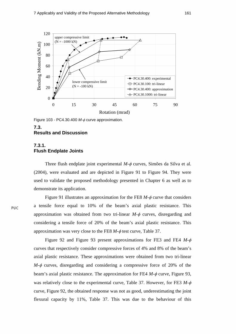
Figure 103 - PC4.30.400 M- curve approximation.

7.3.Results and Discussion

7.3.1.Flush Endplate Joints

Three flush endplate joint experimental M- curves, Simões da Silva et al.

(2004), were evaluated and are depicted in Figure 91 to Figure 94. They were

used to validate the proposed methodology presented in Chapter 6 as well as to

demonstrate its application.

Figure 91 illustrates an approximation for the FE8 M- curve that considers

a tensile force equal to 10% of the beam’s axial plastic resistance. This

approximation was obtained from two tri-linear M- curves, disregarding and

considering a tensile force of 20% of the beam’s axial plastic resistance. This

approximation was very close to the FE8 M- test curve, Table 37.

Figure 92 and Figure 93 present approximations for FE3 and FE4 M-

curves that respectively consider compressive forces of 4% and 8% of the beam’s

axial plastic resistance. These approximations were obtained from two tri-linear

M- curves, disregarding and considering a compressive force of 20% of the

beam’s axial plastic resistance. The approximation for FE4 M- curve, Figure 93,

was relatively close to the experimental curve, Table 37. However, for FE3 M-

curve, Figure 92, the obtained response was not as good, underestimating the joint

flexural capacity by 11%, Table 37. This was due to the behaviour of this

7 Applicably and Validity of the Proposed Alternative Methodology 162

experimental curve when compared to the others. It is possible to observe in

Figure 88 that there is an increase in the flush endplate joint moment capacity

from FE1 M- curve (N = 0% Npl) to FE7 M- curve (N = -20% Npl). However,

within this range, with a 4% beam’s compressive plastic resistance the flexural

capacity is larger than the maximum moment obtained with the 8% test.

Following this increasing tendency in the joint flexural capacity registered from

FE1 (N = 0% Npl) to FE7 (N = -20% Npl), the maximum moment obtained with

FE4 (N = -8% Npl) should be larger than FE3 (N = -4% Npl). A possible reason for

this perturbation in the experimental results might be related to problems with the

FE3 experimental test such as measuring errors or assembly eccentricities.

In general, the predictions of the M- curves using the methodology

proposed in Chapter 6 provided accurate correlations with the test curves from

Simões da Silva et al. (2004) as can be seen in Table 37.

Table 37 - Comparisons between the experimental and the proposed methodology in

terms of initial stiffness and design moment capacity for flush endplate joints.

Tests Initial Stiffness (kNm/rad) Design Moment (kNm)Appr Exp Appr/Exp % Appr Exp Appr/Exp %

FE3 (N=-4% Npl) 8097 10132 0.80 20 74 83 0.89 11FE4 (N=-8% Npl) 8147 10903 0.75 25 75 75 1.00 0

FE8 (N=+10% Npl) 4568 5403 0.85 15 64 68 0.94 6

Note: Negative percentage means overestimated value in % whilst positive percentage indicates underestimated value in %. Joint design moment was determined according to Eurocode 3:1-8 (2005), through the intersection between two straight lines, one parallel to the initial stiffness and another parallel to the moment-rotation curve post-limit stiffness.

7.3.2.Column Bases

Regarding the tests performed by Guisse et al. (1996), four baseplate

experimental M- curves were evaluated and are presented in Figure 100 to Figure

103. Figure 100 draws the prediction of PC2.15.600 M- curve for a compressive

force of 600 kN, by using two reference M- curves: PC2.15.100 and

PC2.15.1000. It is possible to note the very close approximation reached at the

evaluated points: 2/3Md, Md and 1.1Md. On the other hand, the initial stiffness was

rather erratic being estimated to be 44% (Table 38) smaller than the experimental

one. This fact occurred because the point 2/3Md, i.e. the first point of the

approximated M- curves, is located above the onset point of physical separation

of the plate and the concrete in the tensile zone. Therefore, the point 2/3Md was

7 Applicably and Validity of the Proposed Alternative Methodology 163

just able to capture the initial stiffness final change not considering the initial

stiffness before the separation of the steel plate and the concrete base.

Figure 101 presents the PC2.30.600 M- curve approximation for a

compressive force of 600 kN, by utilising the reference M- curves: PC2.30.100

and PC2.30.1000. A reasonable approximation was obtained for this M- curve,

however the initial stiffness was underestimated by 32% and the flexural capacity

was slightly under predicted by 5%, Table 38.

Figure 102 demonstrates the PC4.15.400 M- curve prediction for a

compressive force of 400 kN, by employing the base M- curves: PC4.15.100 and

PC4.15.1000. A good correlation between the experimental tests and numerical

results was obtained. Unlike the others results, the initial stiffness and the design

bending moment were over predicted by 26% and 3%, respectively.

Finally, Figure 103 presents the estimation of the PC4.30.400 M- curve for

a compressive force of 400 kN, by having as basis PC4.30.100 and PC4.30.1000

M- curves. This case did not produce an accurate prediction of the M- curve,

Table 38. However, this fact may be justified due to the occurrence of the column

end section yielding as well as column flange local plate buckling. In others

words, the column capacity was reached before achieving the baseplate joint

flexural capacity.

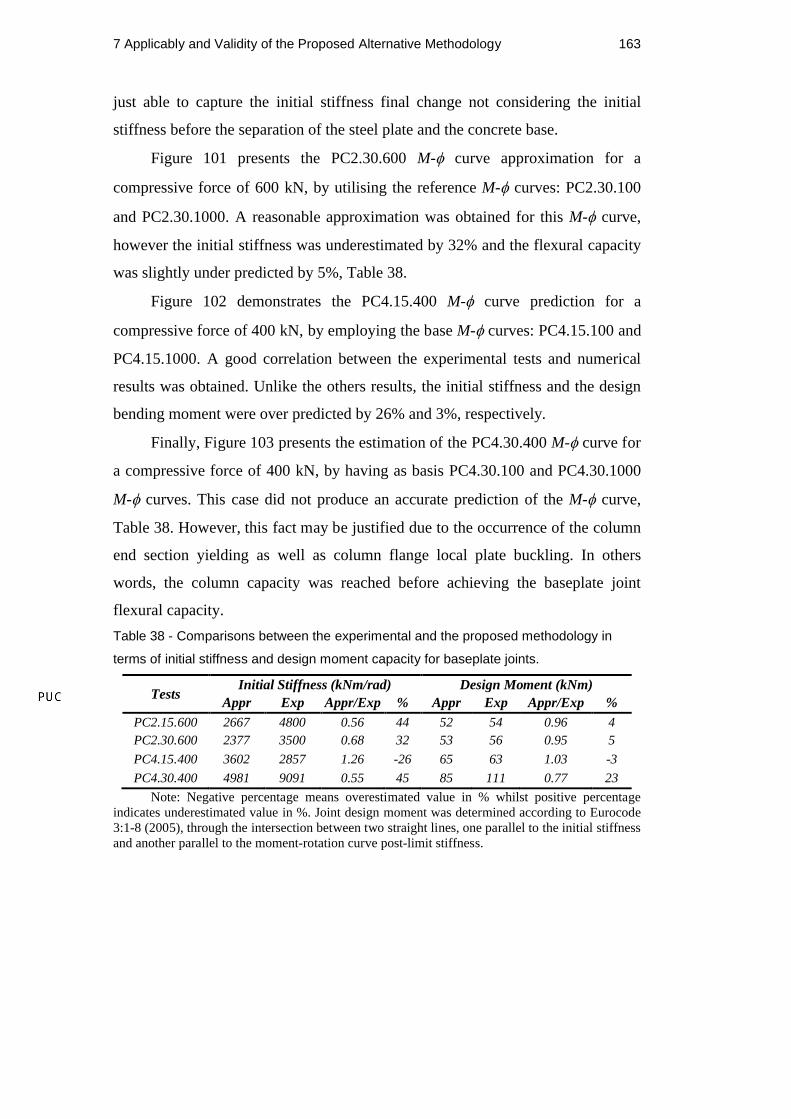
Table 38 - Comparisons between the experimental and the proposed methodology in

terms of initial stiffness and design moment capacity for baseplate joints.

TestsInitial Stiffness (kNm/rad) Design Moment (kNm)

Appr Exp Appr/Exp % Appr Exp Appr/Exp %

PC2.15.600 2667 4800 0.56 44 52 54 0.96 4PC2.30.600 2377 3500 0.68 32 53 56 0.95 5

PC4.15.400 3602 2857 1.26 -26 65 63 1.03 -3

PC4.30.400 4981 9091 0.55 45 85 111 0.77 23

Note: Negative percentage means overestimated value in % whilst positive percentage indicates underestimated value in %. Joint design moment was determined according to Eurocode 3:1-8 (2005), through the intersection between two straight lines, one parallel to the initial stiffness and another parallel to the moment-rotation curve post-limit stiffness.