7 1551 hsd10102_1_b2_rf_dimensioning_methodology_p4

ERICSSON WCDMA RADIO ACCESS NETWORK

7/1551-HSD 101 02/1 Rev B2 2004-11-30 ERICSSON INTERNAL INFORMATION – COMMERCIAL IN CONFIDENCE 1(27)

RF DIMENSIONING METHODOLOGY GUIDELINE

Ericsson AB 2004

The contents of this product are subject to revision without notice due to continued progress in methodology, design and manufacturing.


2(27) ERICSSON INTERNAL INFORMATION – COMMERCIAL IN CONFIDENCE 7/1551-HSD 101 02/1 Rev B2 2004-11-30

Revision history Rev Date Description

A 2000-06-30 First release

B 2002-08-19 Major rework

B1 2003-01-19 Change of classification, new notation.

B2 2004-11-30 Pdf version. No technical or editorial changes



Contents 1 Introduction .......................................................................5 1.1 Overview ...............................................................................................5 1.2 Abbreviations ........................................................................................5

2 Dimensioning assumptions..............................................6 2.1 Introduction ...........................................................................................6 2.2 Propagation model ................................................................................6 2.3 Traffic model .........................................................................................6 2.4 Interference ...........................................................................................7 2.5 Hardware...............................................................................................7 2.6 RN Functionality....................................................................................7

3 Methodology ......................................................................8 3.1 The dimensioning process ....................................................................8 3.2 Input definition.......................................................................................9 3.3 Air interface dimensioning...................................................................10 3.4 Hardware dimensioning ......................................................................16 3.5 Evaluation of results............................................................................17

4 Calculations .....................................................................18 4.1 Loading................................................................................................18 4.2 Traffic ..................................................................................................22

5 References .......................................................................24 Appendix A – DTX gain........................................................25 Appendix B – Parameter dependencies.............................27



1 Introduction

1.1 Overview The scope of this document is to provide a method to dimension a WCDMA radio network given some basic constraints. The focus is to tie together information and methods in several guidelines [1 to 3], and to present a coherent method for the entire RN dimensioning process. Step by step instructions are provided throughout the document to guide the reader in the dimensioning process.

The first part describes the process and several methods that can be used in the dimensioning. The second part of the document deals with fundamental concepts and formulas needed for the dimensioning.

1.2 Abbreviations 2G 2nd Generation mobile telephony systems 3G 3rd Generation mobile telephony systems AF Activity Factor ASC Antenna System Controller ASE Air Speech Equivalents CE Channel Elements COST European Co-Operation within the field of Scientific and Technical

research DCH Dedicated Channel DCCH Dedicated Control Channel DTX Discontinuous transmission DL Downlink GoS Grade of Service HW Hardware ITU International Telecommunications Union MCPA Multi Carrier Power Amplifier RAB Radio Access Bearer RB Radio Bearer RBS Radio Base Station RFI Request For Information RFQ Request for Quotation RN Radio Network TN Transport Network TEMS Test Mobile System UE User Equipment UL Uplink WCDMA Wideband Code Division Multiple Access



2 Dimensioning assumptions

2.1 Introduction This document aims at providing simple and coherent methods for calculating the number of RBSs and their configurations that is needed in a roll-out project. If all characteristics in the radio interface have to be considered, this can become rather complex. The radio network dimensioning is aimed to support engineers for quick and rough calculations with reasonable accuracy in the design phase before starting up planning tools or in the tender process.

To obtain the necessary computational efficiency, certain simplifications have to be made in the assumptions behind the dimensioning process. It is the aim of this chapter to outline those assumptions. It is important for the engineer to be aware of exactly which simplifications that have been made.

2.2 Propagation model Throughout the dimensioning a very simplified propagation model is used. It is based on a flat earth (no terrain height variations) and a compensation factor for the environment type.

2.3 Traffic model

Homogeneous traffic distribution

In the dimensioning it is assumed that the offered traffic is distributed homoge-neously throughout the network. This assumption makes it possible to calculate the maximum traffic carried, on a cell and system level.

The drawback with this assumption is that in a real network this is not the case. There will be hotspot areas and areas with little traffic. These variations are very difficult to model in a dimensioning exercise without the methods becoming overly complex. If irregularities in the traffic distribution have to be considered, it is recommended to use a WCDMA planning tool, such as TEMS CellPlanner, where these effects can be modeled.

Homogeneous user distribution

It is assumed that users within a cell are evenly distributed. This is a valid assumption for low bit rate applications that do not require much capacity. An example of such an application is the speech service, where many users can be allowed in the cell, giving an even user distribution a statistical confidence.

However, for high bitrate services only a few users can be served at a time. In this case the position within the cell will matter. Thus, in reality there will be large variations especially regarding DL power consumption. Again, this can be modeled in a WCDMA planning tool.



Impact of DTX

In the air interface there is a gain due to DTX for each radio bearer. For speech services, this is modeled as an increase in the pole capacity. Because of signaling overhead it is not possible to fully utilize the “gain” due to the activity factor. For speech the gain is typically around 70-100%.

See the appendix for DTX gain for different RABs.

2.4 Interference

Hard blocking

Due to the assumptions of homogeneous traffic distribution and homogeneous user distribution, the interference in the air provides a hard blocking limit in this model. Once the interference limit has been passed the system can no longer be considered to be capable of sustaining additional traffic.

In reality there will be soft blocking in a WCDMA network. Admission and congestion control use interference measurements in the UL and power usage in the DL for decisions whether to accept new traffic or not.

Multiple carriers

Multiple carriers in a cell will increase capacity. In the dimensioning there is no drawback to adding an additional carrier. Full utilization of the new carrier is assumed with no regard to adjacent channel interference, use of compressed mode or lack of load sharing.

Hexagonal cells, equidistant sites

The dimensioning model assumes a network with hexagonal cells and equidistant sites, ignoring the effects of off grid site locations. Examples of these effects would otherwise be higher common channel power needed to provide coverage, higher DCH channel power when in coverage holes, pilot pollution issues, and lower capacity due to increased interference levels.

2.5 Hardware The hardware consists of a fixed amount of resources and is thus subject to hard blocking. The RBS has the possibility to pool capacity resources within one cabinet. This means that when dimensioning the RBS the total site traffic has to be considered.

2.6 RN Functionality

Capacity management

The current dimensioning model assumes an ideal capacity management that has the ability to move and add users in order to have optimal usage of the hardware and air interface. Although this is not strictly true, for average type dimensioning



activities that this guideline is aimed for this assumption is sufficient. The capacity management functions are aimed at keeping the system stable and efficient in a dynamic situation. The dimensioning activity does not intend to model this behavior.

Handover

The handover parameters used in the dimensioning are based on system simulations with realistic input. When data from the field becomes available these parameters will be updated.

Compressed mode

Currently there is no consideration of the effect of compressed mode in the dimensioning methodology.

Channel switching

An ideal channel switching functionality is assumed that has the ability to switch users up and down in an optimal fashion. Down switch delay is considered in the traffic input.

3 Methodology

3.1 The dimensioning process The dimensioning process can be roughly divided into four main blocks as shown in Figure 1.

1. INPUTANALYSIS

2. AIR INTERFACEDIMENSIONING

3. HARDWAREDIMENSIONING

4. EVALUATION

Main input:•Customer•RFI/RFQ

StrategyOutput:•TN Dim.•Pricing

Figure 1. Radio network dimensioning process

1. Input analysis This part of the dimensioning process considers the data received from the customer through RFI/RFQ or similar. In this part of the process services to be used, coverage requirements, quality of service and traffic profile are calculated and decided upon.

2. Air interface dimensioning This is the core of the dimensioning where the required amount of sites is calculated.

3. Hardware dimensioning Here the required amount of hardware is calculated in order to support the calculated air interface capacity, when certain quality constraints of hardware availability are given.



4. Evaluation An evaluation is always needed after the dimensioning to make sure that the values is reasonable and that they are in line with customer expectations. Part of the evaluation is also to document results in a way that is easy to under-stand.

3.2 Input definition

3.2.1 General

This section describes the input parameters for a dimensioning project. Careful analysis of the input data is essential for a successful result. Accurate definitions of the input values give more realistic and useful output values.

Most parameters considered in this phase of the dimensioning are similar to those used in 2G dimensioning, e.g. propagation, site-specific parameters and coverage degree. Others are specifically dependent on WCDMA such as radio bearers and soft handover parameters. This section will not deal with actual parameter values as these are described in other guidelines [1 to 5].

3.2.2 Environment and coverage

The environment is specified by the area type and by the propagation model. • Area –given in km2 • Propagation model parameters [1] – (in e.g. Okumura-Hata and Walfish

models) – It is important to remember that Okumura-Hata parameters are not valid for cell ranges less than 1 km. Thus, when calculating using automatic tools the actual cell range has to be checked.

• Channel model – this parameter has an impact on the Eb/No values and is therefore important both for cell coverage and cell capacity. The channel model to select will depend on the environment for the given area [2]

• Coverage degree – indoor/outdoor

3.2.3 Service characteristics

This input defines which RAB and RB to be used with which service and what UE type is used with the services [3]. • RABs • GoS • UE type – power, UE antenna gain, UE antenna height

3.2.4 Subscriber density and subscriber behavior

This type of input data is central to the traffic part of the calculations. It describes user behavior. The operator must supply these values directly or indirectly as they depend on the predictions for subscriber density and strategies for subscriber



behavior. In order to obtain a high degree of confidence in the end result, the accuracy and reliability of these parameters is important, since these values propagate throughout the entire dimensioning. If real data is available this can be used with great benefit to find an accurate starting point of the dimensioning exercise. • Subscriber density – number of subscribers per area • Traffic density – traffic per subscriber and RAB • Activity factor • Body loss

3.2.5 System design data

System design parameters are items that the engineer can have control over when making a design, or they are given as characteristics of the system. • Retransmissions • Handover – (users in soft, softer soft/softer handover) • Site configuration – Antennas, feeders, ASC, noise factor • Bandwidth – number of carriers • Load

3.2.6 Determining the average user profile

It is convenient to define an “average user” to obtain a good feeling for the traffic distribution generated by the service provider. The “average user” defines the traffic for all services during the busy hour. This abstraction makes it seem that a user is using several simultaneous services at the same time. Naturally this will not be the case in reality. For dimensioning purposes it is however useful, as it enables the reduction of complex multiple input data fields into a standardized input matrix.

3.3 Air interface dimensioning

3.3.1 General

The air interface dimensioning aims to find the required amount of sites, the capacity per cell and the load, based on the constraints in the air interface. Depending on the given input parameters and the degree of freedom in the dimensioning there are a number of approaches available. In this section the four most common methods are presented. Each method is described by an objective for the dimensioning, a list of design constants showing which parameters are fixed at a given value and a description of the method.

In general the output from all air interface dimensioning should be: • Number of sites • Site configuration



• Traffic carried per site and per cell • Capacity per site and per cell

Formulas to calculate loading can be found in section 4.1. Link budget calculations for UL and DL are described in detail in the Coverage and Capacity Guideline [2]. Methods to calculate offered traffic are given in section 4.2.

3.3.2 Variable load dimensioning

Objective: • To find minimum number of sites

Design input constants: • Offered network traffic • Area coverage • One configuration

Description

This is the classical dimensioning method where there is full freedom to find the optimal number of sites by varying the load per cell.

Two series of calculations with varying load per cell are performed. In one, only the requirement on coverage degree is taken into consideration, in the other only the requirement on network capacity. A high load yields many sites to fulfill the coverage requirement (first series of calculations) but few sites for the capacity requirement (second series of calculations), and vice versa for a low load. By modifying the number of users per cell it is possible to find the required amount of sites to fulfill both the coverage and capacity requirements. This is the optimal number of sites. An example is shown in Figure 2 below.

10% 20% 30% 40% 50% 60% 70% 80%

Load

Num

ber o

f site

s

UL coverage

DL coverage

Capacity

Optimal site count

Figure 2 The number of sites required for coverage and capacity as a function of load settings

Although this method gives the optimal number of sites it poses some questions regarding network growth. For example let us say that in the first year the number of sites was found at a DL load of 35%. The second year the expected load with



the same site count is 45%. Obviously more sites are required but how will these sites fit into the network and will the current sites have to be moved?

In many cases this type of questions are not an issue as the most interesting aspect of the dimensioning activity is to get a good approximation of the number of sites required per year. If it is considered that sites in reality are not evenly distributed, this approach is quite useful.

The following diagram illustrates a step-by-step approach in order to find the optimal site count.

Start values

Balanced?

N

Y

Sites forcapacity

Sites for DLcoverage

Sites for ULcoverage

UL load DL load

Finished!

Subs/cell

Input data

Max (UL,DL)

Figure 3 Method to find the optimal site count, balancing UL and DL coverage and capacity



3.3.3 Fixed site dimensioning

Objective: • To find capacity per cell • To find carried traffic per cell • To check to make sure coverage is supported

Design input constants: • Number of sites in the system

Description

This type of dimensioning is interesting when some infrastructure exists and the number of sites given as a constant. Typically the result of this method can be used as an input for expansion calculations like sectorization, carrier expansion and need for hot spot sites.

Finding maximum capacity

With a given amount of sites and given coverage criteria, the maximum allowed load that the system can support is calculated with the following steps. 1. Find the actual cell range (from the given number of sites and area) 2. Use the UL link budget to calculate the max allowed noise rise that yields the

UL load. 3. Use the DL curves and the DL margin to find the maximum allowed DL load. 4. Find the maximum number of users for these load constraints. 5. Find the maximum capacity per cell.

Coverage check 1. Calculate the traffic per cell 2. Calculate the average load due to

conversational traffic, the conversational load at the GoS criteria and best effort load due to the best effort traffic for UL and DL based on the actual traffic

3. Calculate the total load as in equation 2. 4. Check to make sure that the load is less

than or equal to maximum allowed load.

Start

End

Input

Traffic per cell

UL load DL load

Load ok?

Y

N

Figure 4 Calculating capacity for fixed number of sites



3.3.4 Fixed load dimensioning

Objective: • To find the minimum number of sites • To find capacity per cell

Design input constants: • Load • System traffic • RBS configuration

Description

In this method the load is kept constant in the dimensioning, acting as a constraint in the dimensioning. The objective is to find the number of sites required with the fixed load, taking into consideration the traffic in the system.

There are two cases to consider • the number of sites required to handle the traffic demand and • the number of sites required to handle the load constraint.

These two cases will not always be equal. In some instances, the traffic demand will cause a capacity limitation, requiring more sites than the basic load constraint. In other cases traffic demand is low resulting in a system that is coverage limited.

Calculating the number of sites with given traffic and load as constants 1. Choose number of users 2. Calculate traffic per cell 3. Calculate average load Qave, conversational load Qc

and best effort load Qbe and compare with the the fixed input load Ldesired

4. If max(Qc, Qave+Qbe) > Qdesired , then decrease the number of users; If max(Qc, Qave+Qbe) < Qdesired , then increase the number of users

5. At equilib

rium calculate the number of sites required for capacity and note the number of users per cell as this will indicate max capacity per cell.

Calculating the number of sites assuming fixed load only

This method can be used to find the required amount of sites if the load is fixed. With a given load the noise rise in UL can be calculated yielding an UL range. The DL curves can then be used to find the DL range together with a DL margin. In contrast to the previous case this assumes that the given load is what is required. No consideration is taken to actual offered traffic.

Figure 5 Calculating the number of sites required for a fixed load

Start

End

Input

Subscribers per cell

UL load DL load

Load ok?

Y

N



1. Set up an UL linkbudget and calculate DL margin

2. Find the UL and DL range Rul, and Rdl 3. Find the cell range: min(Rul, Rdl) 4. Calculate the number of sites

Alternatively it is possible to set up a DL link budget to find the DL range.

Considering coverage and capacity criteria

Once the calculation of the two cases has been completed the required number of sites can be found by taking the maximum value of the two cases. Capacity per cell is given implicitly in the first case.

3.3.5 Dimensioning with a variable number of carriers

Objective • To find the optimal site configuration mix • To find the capacity per cell per configuration

Design input constants • The number of sites or fixed load • System traffic

Description

This method is ideal for expansion calculation of an already existing network or a network where a fixed load constraint has been given. Although limitations have been set up regarding load (or number of sites) it is possible to vary the site configuration to get an optimal network. In comparison to the other methods two additional assumptions assuming perfect load sharing between carriers must be made: • Same load on all carriers • All carriers within one cell are seen as one unit which allows for trunking

efficiency

Finding an optimal site configuration

Below is a step-by-step method to calculate a system that uses a variable number of carriers.

Figure 6 Flow to calculate sites required for coverage

Start

End

Input

Range is min of UL and DL range

UL range DL range

UL linkbudget DL linkbudget



1. Calculate the required load using the method for fixed number of sites (section 3.3.3).

2. Calculate the required amount of sites using the method for fixed load (section 3.3.4).

3. Calculate the cell capacity for all configurations that are relevant in the dimensioning, e.g. 3x1, 3x2 and 3x3 configurations. Use the method for fixed load (section 3.3.4).

4. Calculate the total offered system traffic. 5. Calculate the system capacity by summing up the

capacity for all individual sites. 6. In case the system capacity is less than the total offered

traffic, then increase the number of carriers on one site and redo step 5. If all sites have maximum number of carriers and there is still a capacity limitation then increase the number of sites.

3.3.6 Treatment of micro cells and pico cells

A micro cell can be modeled as a pure capacity relief site meaning that all the offered traffic on the cell can be reduced from the total system traffic. By doing this it is assumed that: • Sites/cells are placed at ideal locations, and are fully loaded during busy hour. • It is known how much capacity a micro cell can take. The current model is

based on a pure micro cell network and no consideration has been taken regarding interference from/to macro layer considering same frequency.

• Perfect capacity management making sure that the micro cell is fully utilized.

3.4 Hardware dimensioning This part of the dimensioning determines to how the RBSs should be configured in terms of capacity. The output of the air interface dimensioning gives the site count and the traffic carried per site. These inputs are used in order to determine the hardware and software capacity configuration in the RBS.

In the RBS there are hardware and software capacity constraints. For dimensio-ning, the software constraints are the main concern although a check should always be made such that there is a sufficient number of HW boards available in the RBS. Calculation of software keys, or channel elements (CE) is described in the Channel Element Guideline [4].

Figure 7 Modifying site configura-tions to match capacity requirements

Start

End

Input

Number of sites per configuration

Y

NCapacity ok?

System capacity calculation



3.5 Evaluation of results

3.5.1 Key indicators

After the radio network design is completed, it is important to review the results to evaluate whether the dimensioning is reasonable or not. This review is used spot errors in the calculations and to capture unreasonable input parameters. There are numerous indicators to study in this evaluation. The following are the five most commonly used.

Sites

The total number of sites, the number of sites per environment and the number of sites per km2 are the most important indicators. Comparisons should be made with other networks (2G and 3G) for similar areas, to make sure that number of sites is in the same range.

Load

The load for the uplink and downlink should be considered. The load must be within the system tolerance levels. If there is a large difference in load between uplink and downlink, this has to be validated.

Traffic

Traffic per cell, traffic per site and differences in uplink and downlink must be checked to see if the traffic mix is reasonable. Indicators of potential errors are services with virtually no traffic per cell. Also, great differences in uplink and downlink can give indications of erroneous assumptions. For example, it is very rare to have a pure downlink service with no uplink traffic at all. There will always be an overhead in the application layer signaling both in uplink and downlink.

Coverage and capacity

An interesting piece of information is whether the system is coverage or capacity limited, and whether it is uplink or downlink limited. For example, in the early phases of a roll out the system should be coverage limited. Another interesting aspect to bring forth is which service that limits the coverage and the capacity. In some cases a high bit-rate service may be the limiting service in a rural environment. This may cause serious coverage problems.

Hardware

A check should be made to see that the RBS can support all the traffic requested and that it maps fairly well with the traffic per site. Questions may perhaps be raised regarding the duty cycle for different services. The packet services are quite hardware intensive at low duty cycles.



4 Calculations

4.1 Loading

4.1.1 Definition

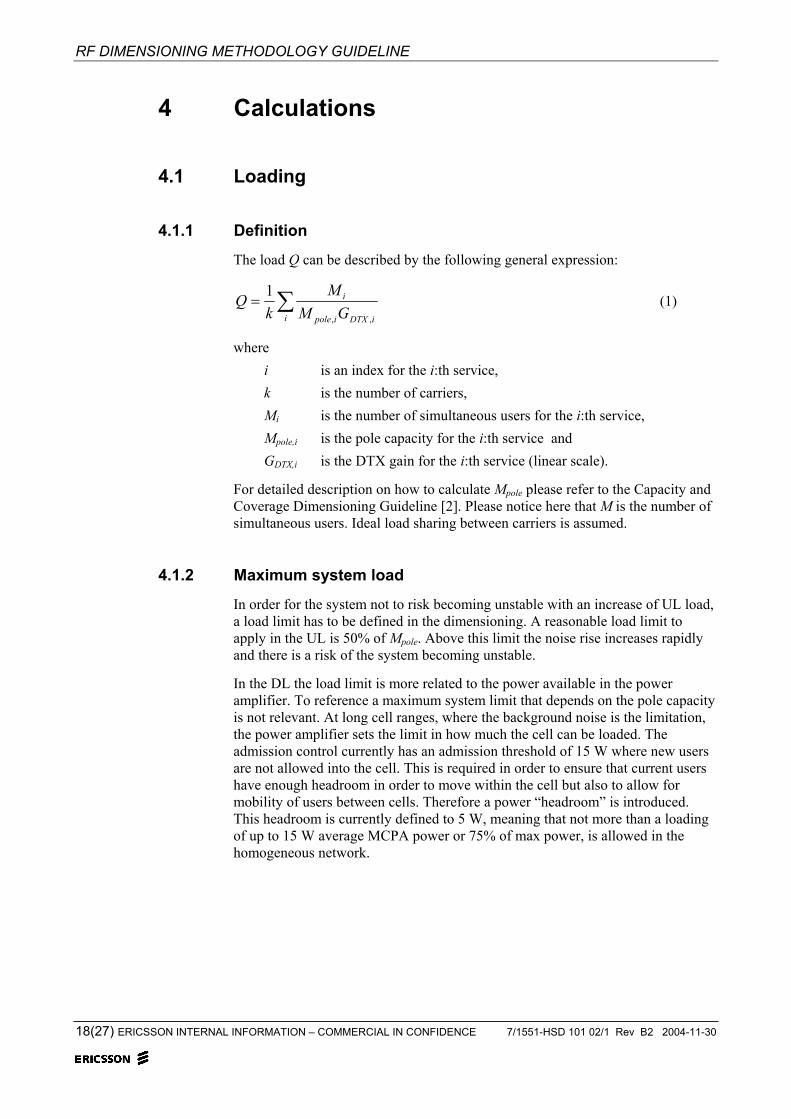
The load Q can be described by the following general expression:

∑=i iDTXipole

i

GMM

kQ

,,

1 (1)

where i is an index for the i:th service, k is the number of carriers, Mi is the number of simultaneous users for the i:th service, Mpole,i is the pole capacity for the i:th service and GDTX,i is the DTX gain for the i:th service (linear scale).

For detailed description on how to calculate Mpole please refer to the Capacity and Coverage Dimensioning Guideline [2]. Please notice here that M is the number of simultaneous users. Ideal load sharing between carriers is assumed.

4.1.2 Maximum system load

In order for the system not to risk becoming unstable with an increase of UL load, a load limit has to be defined in the dimensioning. A reasonable load limit to apply in the UL is 50% of Mpole. Above this limit the noise rise increases rapidly and there is a risk of the system becoming unstable.

In the DL the load limit is more related to the power available in the power amplifier. To reference a maximum system limit that depends on the pole capacity is not relevant. At long cell ranges, where the background noise is the limitation, the power amplifier sets the limit in how much the cell can be loaded. The admission control currently has an admission threshold of 15 W where new users are not allowed into the cell. This is required in order to ensure that current users have enough headroom in order to move within the cell but also to allow for mobility of users between cells. Therefore a power “headroom” is introduced. This headroom is currently defined to 5 W, meaning that not more than a loading of up to 15 W average MCPA power or 75% of max power, is allowed in the homogeneous network.



4.1.3 Conversational, average, and best effort load

Figure 8 illustrates the definitions of conversational, average conversational, and best effort load. Equation 2 defines the dimensioning load Q from these quantities.

Time

Load

Average conversational load

Conversational load

Dimensioning load

Best effort load

Figure 8 Conversational, average conversational and best effort load

),max( beaveragec QQQQ += (2)

where Qc is the conversational load, which models the maximum number of

conversational class users active during the busy hour based on GoS criteria,

Qave is the average conversational load, the load generated by the conversational class bearers on average during the busy hour,

Qbe is the best effort load, the load generated by the interactive (best effort) bearers.

4.1.4 Load due to conversational class traffic

Conversational load for a one bearer service

By assuming a hard capacity limit it is possible to use Erlang B formulas in order to find a blocking probability for conversational class traffic. The number channels Mi required for the service is then

Mi = ErlangB(Acell,i,KGoS) (3)

where Acell,i is the offered traffic for service i, and KGoS is the grade of service in %

From the definition of load it is then straightforward to calculate the conversational load Qc from equation 1.



Conversational load for several bearers using complete partitioning

If it is assumed that the traffic on all RBs peak at exactly the same time it is possible to use complete partitioning of the spectrum. This is what the Erlang B formula implies and this can be applied for each RAB.

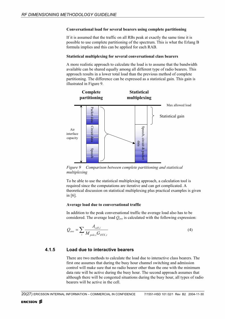
Statistical multiplexing for several conversational class bearers

A more realistic approach to calculate the load is to assume that the bandwidth available can be shared equally among all different type of radio bearers. This approach results in a lower total load than the previous method of complete partitioning. The difference can be expressed as a statistical gain. This gain is illustrated in Figure 9.

SpeechPacket data

Circuit data

Speech, circuit & packet

data

Completepartitioning

Statisticalmultiplexing

Statistical gain

Max allowed load

Airinterfacecapacity

Figure 9 Comparison between complete partitioning and statistical multiplexing

To be able to use the statistical multiplexing approach, a calculation tool is required since the computations are iterative and can get complicated. A theoretical discussion on statistical multiplexing plus practical examples is given in [6].

Average load due to conversational traffic

In addition to the peak conversational traffic the average load also has to be considered. The average load Qave is calculated with the following expression:

∑=i iDTXipole

icellave GM

AQ

,,

, (4)

4.1.5 Load due to interactive bearers

There are two methods to calculate the load due to interactive class bearers. The first one assumes that during the busy hour channel switching and admission control will make sure that no radio bearer other than the one with the minimum data rate will be active during the busy hour. The second approach assumes that although there will be congested situations during the busy hour, all types of radio bearers will be active in the cell.



The first method results in many users in the system but with relatively low throughput per user. The second method yields fewer users in the system but in contrast these users get maximum possible throughput.

Only minimum data rate bearer during busy hour

This method is the simplest for manual calculations. The only thing to consider is the minimum data rate bearer that is allowed, and then to map all traffic onto this one. The best effort load can then be calculated with the following two expressions:

PFDTXpole,minRB

be KGM

MQ = (5)

∑∑ +=+=i

icellreti

iuserretcells

subs AKAKnn

M ,, )1()1( (6)

where KPF is the peak factor considering that it is not possible to utilize the

entire traffic channel, Mpole,minRB is the pole capacity for the minimum data rate radio bearer, Kret is the expected retransmission ration, nsubs is the total number of subscribers, ncells is the total number of cells and Auser,i is the offered traffic for user with service i.

Here it is assumed that during the busy hour the admission and congestion control functions will never allow best effort users onto a radio bearer with higher data rate than the minimum configuration. It is assumed that the cell is constantly congested, or loaded in such a way that there is no room for higher data rate bearers. This is a conservative approach especially when low bearer rates are available for the interactive class services.

No bearer restriction during busy hour

This method assumes that even during busy hour the best effort bearer will not be constrained to the lowest data rates. This means that it is assumed that there are no limitations due to power, ASE or codes during the busy hour. In a low load scenario this is a valid assumption, but in cases with high load, including a large portion of conversational class traffic, this may not be true. The following formula can be used to calculate the best effort load.

∑=i iDTXipole

PFbe GMipMKQ

,,

)( (7)

where p(i) is the probability that the simultaneous user is expected to be on RB i (relative time spent on RB i). The DTX gain GDTX is a function of the activity factor (AF) and is described in more detail in Appendix A [2].

The number of simultaneous users M can be calculated with the following equation:



TA

RYnn

M icell

sessionpeak

pagesubs ,==τ

(8)

where npage is the number of downloaded pages per subscriber, Y is the payload, Rpeak is the session peak rate, τsession is the session efficiency and T is the average throughput for a typical user [3].

4.2 Traffic

4.2.1 Air interface

Offered traffic per user

In order to calculate the average user profile all total offered traffic in the system per environment must be mapped to each subscriber. The following equation calculates the offered traffic per user for RAB type i:

subs

itotaliuser n

AA ,

, = (9)

Auser is calculated in the average user profile.

If A is given in bps the following expression can be used

user

ibpsuseriuser R

AA ,_

, = (10)

where Ruser is the data rate for the RAB.

Offered traffic per cell

Using the offered traffic per user, the offered traffic per cell Acell,i becomes:

cells

iusersubsicell n

AnA ,

, = (11)

Compensation for retransmission

For interactive class bearers the simulations of Eb/Io values have used a block error rate probability. This block error rate will cause retransmissions in the real life system. This has to be compensated for in the traffic calculations.



)1(,, retiusercells

subsicell KA

nn

A += (12)

The retransmission factor Kret for the COST259 RABs is currently 1%. For older ITU channel models retransmission is 10%.

Compensation for bursty behavior of interactive class traffic

There is no scheduling of the packet traffic on interactive class bearers, only a random access scheme. Therefore it is probable that the average channel allocated for interactive class traffic will not be enough. A peak factor KPF is introduced to compensate for this.

PFretiusercells

subsi KKA

nn

A )1(, += (13)

The peak factor can be viewed as a channel utilization factor. A recommended value to use is 1.4, which is equivalent to 70% channel utilization. This factor is not needed for conversational class data traffic since in those cases a GoS has been used to compensate for the peak traffic.

4.2.2 Hardware

Offered traffic per site

When calculating hardware resources or channel elements the traffic or simultaneous users per site is of interest. The RBS is constructed in such a way that it pools hardware resources from all cell carriers. It is therefore possible to treat the site as one entity. The offered trafic per site and RAB Asite,i is

site

iusersubsisite n

AnA ,

, = (14)

where nsite is the number of sites, and Auser,i is given by equation 9.

Compensation for retransmission

A compensation for retransmissions yields

)1(,, retiusersite

subsisite KA

nn

A += (15)

Compensation for activity factor

The activity factor or the DTX gain GDTX is considered in the air interface calculations. For the hardware the key parameter is the number of simultaneous users for each service. A low activity factor (high DTX gain) means that the air interface can handle more simultaneous users and hence the hardware requirements will increase.



UL/DL considerations

In the hardware the number of simultaneously connected users consume hardware both in UL or DL regardless if they are actively transmitting or not. This is in contrast to the air interface where the UL and DL can be treated separately.

5 References 1 Radio Wave Propagation Guideline, 16/1551-HSD 101 02/1 2 Capacity and Coverage dimensioning, 17/1551-HSD 101 02/1 3 Air interface traffic modeling, 61/1551-HSD 101 02/1 4 Channel Element Dimensioning Guideline, 62/1551-HSD 101 02/1 5 Common Control Channel Guideline, 63/1551-HSD 101 02/1 6 Statistical Multiplexing, Theory and Implementation, ERA/FN/R-01:0087



Appendix A – DTX gain Due to overhead in signaling on layer 1, the gain achieved from low activity is not ideal. This is already evident for a speech RAB that has a DTX gain GDTX of 1.5 at an activity factor of 50%. In an ideal case the gain should have been 2. Figures A1 and A2 show a graphs of the uplink DTX gain at different activity factors. Tables A1 and A2 give some numerical values. In the figures and tables the DTX gain is related to capacity at 100% activity on the DCH and on the DCCH. The figures include a 10% DCCH activity and hence the DTX gain may be larger than 1 even for 100% activity factor of the DCH.

0

1

2

3

4

5

6

7

8

9

10

10 20 30 40 50 60 70 80 90 100Activity factor

DTX

gai

n

Speech

CS64CS57.6, I64

Ideal

Figure A1. Uplink DTX gain

Table A1. Uplink DTX gain

Load Speech CS64 I64 CS57.6 Ideal

10% 2.6 3.5 3.4 3.4 10.0

20% 2.3 2.8 2.7 2.7 5.0

30% 2.0 2.3 2.3 2.3 3.3

40% 1.8 2.0 1.9 2.0 2.5

50% 1.7 1.7 1.7 1.7 2.0

60% 1.6 1.4 1.4 1.4 1.7

70% 1.4 1.4 1.4 1.4 1.4

80% 1.3 1.3 1.2 1.2 1.3

90% 1.3 1.2 1.1 1.1 1.1

100% 1.2 1.1 1.0 1.1 1.0



0

1

2

3

4

5

6

7

8

9

10

10% 20% 30% 40% 50% 60% 70% 80% 90% 100%Activity factor

DTX

gai

n

Speech

CS 64,I64,CS57.6

I128

I384

Ideal

Figure A2. Dowlink DTX gain

Table A2. Downlink DTX gain

Load Speech CS64 I64 I128 I384 CS57.6 Ideal

10% 4.3 4.7 4.7 6.3 6.9 4.7 10.0

20% 3.4 3.4 3.4 4.0 4.2 3.4 5.0

30% 2.7 2.6 2.7 2.9 3.0 2.7 3.3

40% 2.3 2.2 2.2 2.3 2.3 2.2 2.5

50% 2.0 1.8 1.8 1.9 1.9 1.9 2.0

60% 1.8 1.6 1.6 1.6 1.6 1.6 1.7

70% 1.6 1.4 1.4 1.4 1.4 1.4 1.4

80% 1.4 1.3 1.3 1.3 1.2 1.3 1.3

90% 1.3 1.2 1.1 1.1 1.1 1.2 1.1

100% 1.2 1.1 1.0 1.0 1.0 1.1 1.0



Appendix B – Parameter dependencies When dimensioning it is convenient to have an overview of how parameters influence the end result. In Figure B1 dependencies of the key parameters in the dimensioning is shown. The gray (or yellow) fields represent individual parameters or groupd of parameters. The white fields represent groups of parameters that are expanded further in the figure.

numb. of sites

Area

Cell range

Load

Cell range UL

Cell range DL

EnvironmentSite config.

Body lossUE

RBCov. req.

Ch. modelPropagation

Load

EnvironmentSite config

Body lossRB

Ch. modelPropagatio

Load

Subs. behavior

Siteconfig.

RBMpole

Traffic/subsSubs/area

numb. of sites

Figure B1 Parameter dependencies in radio network dimensioning

7 1551 hsd10102_1_b2_rf_dimensioning_methodology_p4

Engineering

Transcript of 7 1551 hsd10102_1_b2_rf_dimensioning_methodology_p4