MIT OpenCourseWare http://ocw.mit.edu

6.055J / 2.038J The Art of Approximation in Science and EngineeringSpring 2008

For information about citing these materials or our Terms of Use, visit: http://ocw.mit.edu/terms.

72 72

72 722008-01-14 22:31:34 / rev 55add9943bf1

6.055 / Art of approximation 72

8.3 Drag

Pendulum motion is not a horrible enough problem to show the full benefit of dimensional analysis. Instead try fluid mechanics – a subject notorious for its mathematical and physical complexity; Chandrasekhar’s books [10, 11] or the classic textbook of Lamb [12] show that the mathematics is not for the faint of heart.

The next examples illustrate two extremes of fluid flow: oozing and turbu­

Density ρfl

Viscosity ν

ρobj

R

v

lent. An example of oozing flow is ions transporting charge in seawater (Section 8.3.6).An example of turbulent flow is a raindrop falling from the sky after condens­ing out of a cloud (Section 8.3.7).

To find the terminal velocity, solve the partial-differential equations of fluidmechanics for the incompressible flow of a Newtonian fluid:

∂v 1 + (v·∇)v = −

ρ∇p + ν∇2v, (3 eqns)

∂t

∇·v = 0. (1 eqn)

Here v is the fluid velocity, ρ is the fluid density, ν is the kinematic viscosity, and p is the pressure. The first equation is a vector shorthand for three equa­tions, so the full system is four equations.

All the equations are partial-differential equations and three are nonlinear. Worse, they are coupled: Quantities appear in more than one equation. So we have to solve a system of coupled, nonlinear, partial-differential equations. This solution must satisfy boundary con­ditions imposed by the marble or raindrop. As the object moves, the boundary conditions change. So until you know how the object moves, you do not know the boundary condi­tions. Until you know the boundary conditions, you cannot find the motion of the fluid or of the object. This coupling between the boundary conditions and solution compounds the difficulty of the problem. It requires that you solve the equations and the boundary conditions together. If you ever get there, then you take the limit t →∞ to find the terminal velocity.

Sleep easy! I wrote out the Navier–Stokes equations only to scare you into using dimen­sional analysis and special-cases reasoning. The approximate approach is easier than solv­ing nonlinear partial-differential equations.

8.3.1 Naive dimensional analysis

To use dimensional analysis, follow the usual steps: Choose relevant variables, form di­mensionless groups from them, and solve for the terminal velocity. In choosing quantities, do not forget to include the variable for which you are solving, which here is v. To decide on the other quantities, split them into three categories (divide and conquer):

1. characteristics of the fluid,

2. characteristics of the object, and

3. characteristics of whatever makes the object fall.

73 73

73 732008-01-14 22:31:34 / rev 55add9943bf1

73 8 Special cases

The last category is the easiest to think about, so deal with it first. Gravity makes the object fall, so g is on the list.

Consider next the characteristics of the object. Its velocity, as the quantity for which we are solving, is already on the list. Its mass m affects the terminal velocity: A feather falls more slowly than a rock does. Its radius r probably affects the terminal velocity. Instead of listing r and m together, remix them and use r and ρobj. The two alternatives r and m or r and ρobj

provide the same information as long as the object is uniform: You can compute ρobj from m and r and can compute m from ρobj and r.

Choose the preferable pair by looking ahead in the derivation. The relevant properties of the fluid include its density ρfl. If the list also includes ρobj, then the results might contain pleasing dimensionless ratios such as ρobj/ρfl (a dimensionless group!). The ratio ρobj/ρfl

has a more obvious physical interpretation than a combination such as m/ρflr3, which, ex­cept for a dimensionless constant, is more obscurely the ratio of object and fluid densities. So choose ρobj and r over m and r.

Scaling arguments also favor the pair ρobj and r. In a scaling argument you imagine varying, say, a size. Size, like heat, is an extensive quantity: a quantity related to amount of stuff. When you vary the size, you want as few other variables as possible to change so that those changes do not obscure the effect of changing size. Therefore, whenever possible replace extensive quantities with intensive quantities like temperature or density. The pair m and r contains two extensive quantities, whereas the preferable pair ρobj and r contains only one extensive quantity.

Now consider properties of the fluid. Its density ρfl affects the terminal velocity. Perhaps its viscosity is also relevant. Viscosity measures the tendency of a fluid to reduce velocity differences in the flow. You can observe an analog of viscosity in traffic flow on a multilane highway. If one lane moves much faster than another, drivers switch from the slower to the faster lane, eventually slowing down the faster lane. Local decisions of the drivers reduce the velocity gradient. Similarly, molecular motion (in a gas) or collisions (in a fluid) transports speed (really, momentum) from fast- to slow-flowing regions. This transport reduces the velocity difference between the regions. Oozier (more viscous) fluids probably produce more drag than thin fluids do. So viscosity belongs on the list of relevant variables.

Fluid mechanicians have defined two viscosities: dynamic viscosity η and kinematic vis­cosity ν. [Sadly, we could not use the mellifluous term fluid mechanics to signify a host of physicists agonizing over the equations of fluid mechanics; it would not distinguish the toilers from their toil.] The two viscosities are related by η = ρflν. Life in Moving Fluids [13, pp. 23–25] discusses the two types of viscosity in detail. For the analysis of drag force, you need to know only that viscous forces are proportional to viscosity. Which viscosity should we use? Dynamic viscosity hides ρfl inside the product νρfl; a ratio of ρobj and η then looks less dimensionless than it is because ρobj’s partner ρfl is buried inside η. Therefore the kine­matic viscosity ν usually gives the more insightful results. Summarizing the discussion, the table lists the variables by category.

74 74

74 742008-01-14 22:31:34 / rev 55add9943bf1

74 6.055 / Art of approximation

The next step is to find dimensionless groups. The Buck- Var Dim Whatingham Pi theorem (Section 7.6) says that the six vari­ ν L2T−1 kinematic viscosity ables and three independent dimensions result in three ρfl ML−3 fluid density dimensionless groups. r L object radius

Before finding the groups, consider the consequences of v LT−1 terminal velocity

three groups. Three?! Three dimensionless groups pro­ ρobj ML−3 object density

duce this form for the terminal velocity v: g LT−2 gravity

group with v = f (other group 1, other group 2).

To deduce the properties of f requires physics knowledge. However, studying a two-variable function is onerous. A function of one variable is represented by a curve and can be graphed on a sheet of paper. A function of two variables is represented by a sur­face. For a complete picture it needs three-dimensional paper (do you have any?); or you can graph many slices of it on regular two-dimensional paper. Neither choice is appeal­ing. This brute-force approach to the terminal velocity produces too many dimensionless groups.

If you simplify only after you reach the complicated form

group with v = f (other group 1, other group 2),

you carry baggage that you eventually discard. When going on holiday to the Caribbean, why pack skis that you never use but just cart around everywhere? Instead, at the be­ginning of the analysis, incorporate the physics knowledge. That way you simplify the remainder of the derivation. To follow this strategy of packing light – of packing only what you need – consider the physics of terminal velocity in order to make simplifications now.

8.3.2 Simpler approach

The adjective terminal in the phrase ‘terminal velocity’ hints at the physicsthat determines the velocity. Here ‘terminal’ is used in its sense of final,as in after an infinite time. It indicates that the velocity has become con­stant, which happens only when no net force acts on the marble. This

and drag. The terminal velocity is velocity at which the drag, gravitational, and buoyant forces combine to make zero net force. Divide-and-conquer reasoning splits the terminal-

terminal velocity

weight drag buoyancy

line of thought suggests that we imagine the forces acting on the object: gravity, buoyancy,

velocity problem into three simpler problems.

The gravitational force, also known as the weight, is mg. Instead of m we use (4π/3)ρobjr3 – for the same reasons that we listed ρobj instead of m in the table of variables – and happily ignore the factor of 4π/3. With those choices, the weight is

Fg ∼ ρobjr3 g.

terminal velocity

weight drag buoyancy

ρspr3g

75 75

75 752008-01-14 22:31:34 / rev 55add9943bf1

︷ ︸︸ ︷

︸︷︷︸

8 Special cases 75

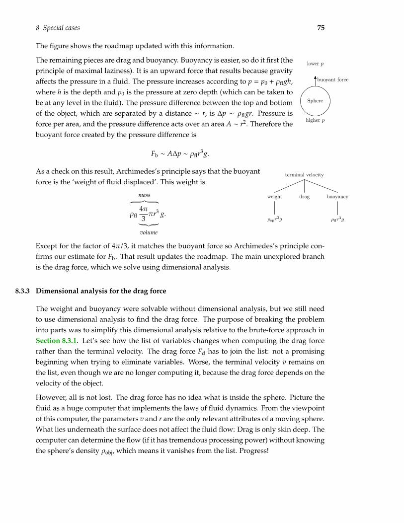
The figure shows the roadmap updated with this information.

The remaining pieces are drag and buoyancy. Buoyancy is easier, so do it first (the

higher p

buoyant force

lower p

Sphere

= p0 + ρfl gh,

Pressure is

principle of maximal laziness). It is an upward force that results because gravity affects the pressure in a fluid. The pressure increases according to pwhere h is the depth and p0 is the pressure at zero depth (which can be taken to be at any level in the fluid). The pressure difference between the top and bottom of the object, which are separated by a distance ∼ r, is ∆p ∼ ρfl gr. force per area, and the pressure difference acts over an area A ∼ r2. Therefore the buoyant force created by the pressure difference is

Fb ∼ A∆p ∼ ρflr3 g.

As a check on this result, Archimedes’s principle says that the buoyant force is the ‘weight of fluid displaced’. This weight is

mass

ρfl 4ππr3 g.

3

volume

terminal velocity

weight drag buoyancy

ρspr3g ρflr3g

Except for the factor of 4π/3, it matches the buoyant force so Archimedes’s principle con­firms our estimate for Fb. That result updates the roadmap. The main unexplored branch is the drag force, which we solve using dimensional analysis.

8.3.3 Dimensional analysis for the drag force

The weight and buoyancy were solvable without dimensional analysis, but we still need to use dimensional analysis to find the drag force. The purpose of breaking the problem into parts was to simplify this dimensional analysis relative to the brute-force approach in Section 8.3.1. Let’s see how the list of variables changes when computing the drag force rather than the terminal velocity. The drag force Fd has to join the list: not a promising beginning when trying to eliminate variables. Worse, the terminal velocity v remains on the list, even though we are no longer computing it, because the drag force depends on the velocity of the object.

However, all is not lost. The drag force has no idea what is inside the sphere. Picture the fluid as a huge computer that implements the laws of fluid dynamics. From the viewpoint of this computer, the parameters v and r are the only relevant attributes of a moving sphere. What lies underneath the surface does not affect the fluid flow: Drag is only skin deep. The computer can determine the flow (if it has tremendous processing power) without knowing the sphere’s density ρobj, which means it vanishes from the list. Progress!

76 76

76 762008-01-14 22:31:34 / rev 55add9943bf1

6.055 / Art of approximation 76

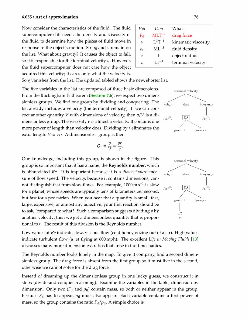
Now consider the characteristics of the fluid. The fluid supercomputer still needs the density and viscosity of the fluid to determine how the pieces of fluid move in response to the object’s motion. So ρfl and ν remain on the list. What about gravity? It causes the object to fall, so it is responsible for the terminal velocity v. However, the fluid supercomputer does not care how the object acquired this velocity; it cares only what the velocity is.

Var Dim What Fd MLT−2 drag force ν L2T−1 kinematic viscosity ρfl ML−3 fluid density r L object radius v LT−1 terminal velocity

So g vanishes from the list. The updated tabled shows the new, shorter list.

The five variables in the list are composed of three basic dimensions. From the Buckingham Pi theorem (Section 7.6), we expect two dimen­sionless groups. We find one group by dividing and conquering. The list already includes a velocity (the terminal velocity). If we can con­coct another quantity V with dimensions of velocity, then v/V is a di­mensionless group. The viscosity ν is almost a velocity. It contains one more power of length than velocity does. Dividing by r eliminates the extra length: V ≡ ν/r. A dimensionless group is then

v vr = .G1 ≡

V ν

Our knowledge, including this group, is shown in the figure. group is so important that it has a name, the Reynolds number, which is abbreviated Re. It is important because it is a dimensionless mea­sure of flow speed. The velocity, because it contains dimensions, can­not distinguish fast from slow flows. For example, 1000 m s−1 is slow for a planet, whose speeds are typically tens of kilometers per second, but fast for a pedestrian. When you hear that a quantity is small, fast, large, expensive, or almost any adjective, your first reaction should be to ask, ‘compared to what?’ Such a comparison suggests dividing v by another velocity; then we get a dimensionless quantity that is propor­tional to v. The result of this division is the Reynolds number.

terminal velocity

weight drag buoyancy

ρspr3g ρflr3gDA

group 1 group 2

terminal velocity

weight drag buoyancy

ρspr3g ρflr3gDA

group 1 group 2

vR

ν

This

Low values of Re indicate slow, viscous flow (cold honey oozing out of a jar). High values indicate turbulent flow (a jet flying at 600 mph). The excellent Life in Moving Fluids [13] discusses many more dimensionless ratios that arise in fluid mechanics.

The Reynolds number looks lonely in the map. To give it company, find a second dimen­sionless group. The drag force is absent from the first group so it must live in the second; otherwise we cannot solve for the drag force.

Instead of dreaming up the dimensionless group in one lucky guess, we construct it in steps (divide-and-conquer reasoning). Examine the variables in the table, dimension by dimension. Only two (Fd and ρfl) contain mass, so both or neither appear in the group. Because Fd has to appear, ρfl must also appear. Each variable contains a first power of mass, so the group contains the ratio Fd/ρfl. A simple choice is

77 77

77 772008-01-14 22:31:34 / rev 55add9943bf1

︸ ︷︷ ︸

8 Special cases 77

.G2 ∝ ρF

fl

d

The dimensions of Fd/ρfl are L4T−2, which is the square of L2T−1. Fortune smiles on us, for L2T−1 are the dimensions of ν. So

Fd

ρflν2

is a dimensionless group.

This choice, although valid, has a defect: It contains ν, which already belongs to the first group (the Reynolds number). Of all the variables in the problem, ν is the one most likely to be found irrelevant based on a physical argument (as will happen in Section 8.3.7, when we specialize to high-speed flow. If ν appears in two groups, eliminating it requires recom­bining the two groups into one that does not contain ν. However, if ν appears in only one group, then eliminating it is simple: eliminate that group. Simpler mathematics – eliminat­ing a group rather than remixing two groups to get one group – requires simpler physical reasoning. Therefore, isolate ν in one group if possible.

To remove ν from the proposed group Fd/ρflν2 notice that the product terminal velocity

weight drag buoyancy

ρspr3g ρflr3gDA

group 1 group 2

vR

ν

Fd

ρflr2v2

of two dimensionless groups is also dimensionless. The first group contains ν−1 and the proposed group contains ν−2, so the ratio

group proposed Fd = (first group)2 ρflr2v2

is not only dimensionless but it also does not contain ν. So the analysis will be easy to modify when we try to eliminate ν. With this revised second group, our knowledge is now shown in this figure:

This group, unlike the the proposal Fd/ρflν2, has a plausible physical interpretation. Imagine that the sphere travels a distance l, and use l to multiply the group by unity:

Fd l Fdl ×

l= ρfllr2v2 . ρflr2v2 ︸︷︷︸

group 1 1

The numerator is the work done against the drag force over the distance l. The denominator is also an energy. To interpret it, examine its parts (divide and conquer). The product lr2 is, except for a dimensionless constant, the volume of fluid swept out by the object. So ρfllr2 is, except for a constant, the mass of fluid shoved aside by the object. The object moves fluid with a velocity comparable to v, so it imparts to the fluid a kinetic energy

EK ∼ ρfllr2v2 .

Thus the ratio, and hence the group, has the following interpretation:

work done against drag .

kinetic energy imparted to the fluid

78 78

78 782008-01-14 22:31:34 / rev 55add9943bf1

( )

78 6.055 / Art of approximation

In highly dissipative flows, when energy is burned directly up by viscosity, the numerator is much larger than the denominator, so this ratio (which will turn out to measure drag) is much greater than 1. In highly streamlined flows (a jet wing), the the work done against drag is small because the fluid returns most of the imparted kinetic energy to the object. So in the ratio, the numerator will be small compared to the denominator.

To solve for Fd, which is contained in G2, use the form G2 = f (G1), which becomes

Fd = f ( vr )

. ρflr2v2 ν

The drag force is then

Fd = ρflr2v2 f vr .

ν

The function f is a dimensionless function: Its argument is dimensionless and it returns a dimensionless number. It is also a universal function. The same f applies to spheres of any size, in a fluid of any viscosity or density! Although f depends on r, ρfl, ν, and v, it depends on them only through one combination, the Reynolds number. A function of one variable is easier to study than is a function of four variables:

A good table of functions of one variable may require a page; that of a function of two variables a volume; that of a function of three variables a bookcase; and that of a function of four variables a library.

—Harold Jeffreys [6, p. 82]

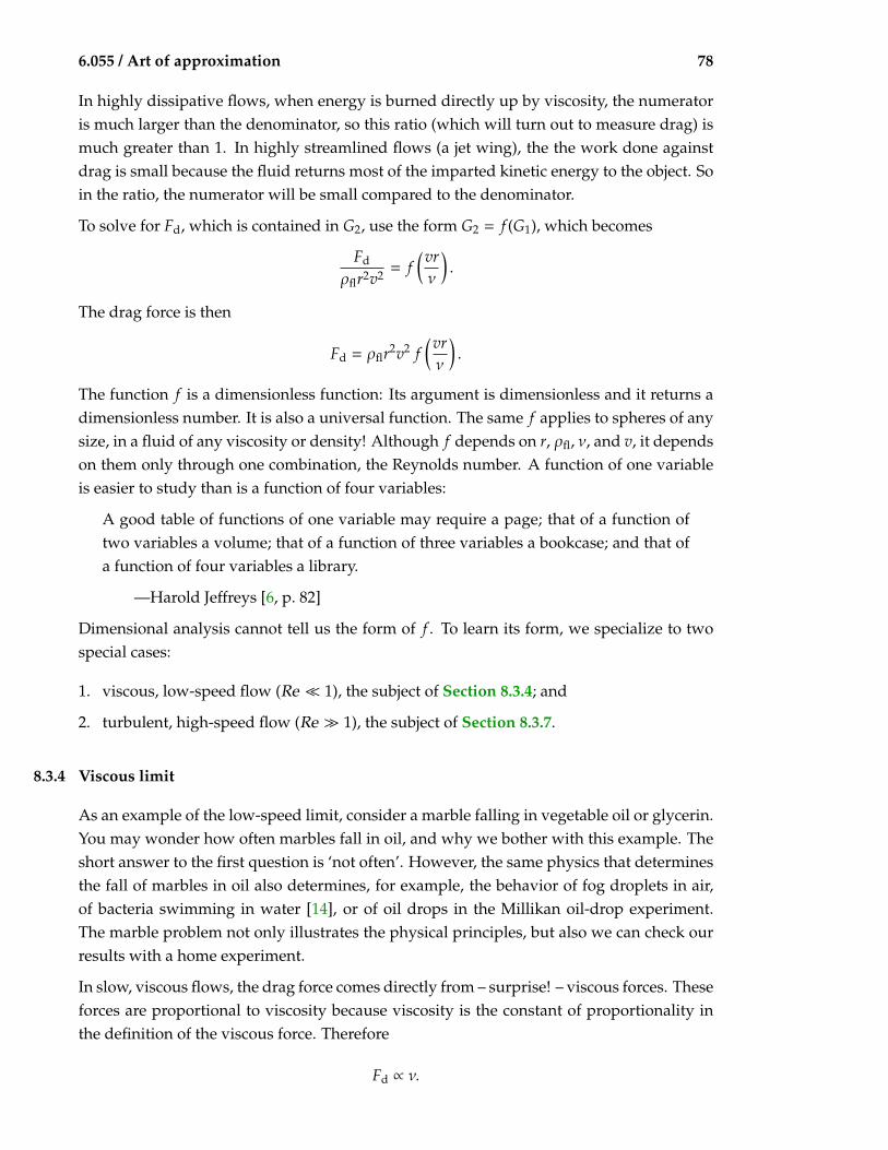
Dimensional analysis cannot tell us the form of f . To learn its form, we specialize to two special cases:

1. viscous, low-speed flow (Re 1), the subject of Section 8.3.4; and

2. turbulent, high-speed flow (Re 1), the subject of Section 8.3.7.

8.3.4 Viscous limit

As an example of the low-speed limit, consider a marble falling in vegetable oil or glycerin. You may wonder how often marbles fall in oil, and why we bother with this example. The short answer to the first question is ‘not often’. However, the same physics that determines the fall of marbles in oil also determines, for example, the behavior of fog droplets in air, of bacteria swimming in water [14], or of oil drops in the Millikan oil-drop experiment. The marble problem not only illustrates the physical principles, but also we can check our results with a home experiment.

In slow, viscous flows, the drag force comes directly from – surprise! – viscous forces. These forces are proportional to viscosity because viscosity is the constant of proportionality in the definition of the viscous force. Therefore

Fd ∝ ν.

79 79

79 792008-01-14 22:31:34 / rev 55add9943bf1

( ) 79 8 Special cases

The viscosity appears exactly once in the drag result, repeated here:

Fd = ρflr2v2 f vr .

ν

To flip ν into the numerator and make Fd ∝ ν, the function f must have the form f (x) ∼ 1/x. With this f (x) the result is

Fd ∼ ρflr2v2 ν = ρflνv. vr

Dimensional analysis alone is insufficient to compute the missing magic dimensionless con­stant. A fluid mechanician must do a messy and difficult calculation. Her burden is light now that we have worked out the solution except for this one constant. The British mathe­matician Stokes, the first to derive its value, found that

Fd = 6πρflνvr.

In honor of Stokes, this result is called Stokes drag.

Let’s sanity check the result. Large or fast marbles should feel a lot of drag, so r and v should be in the numerator. Viscous fluids should produce a lot of drag, so ν should be the numerator. The proposed drag force passes these tests. The correct location of the density – in the numerator or denominator – is hard to judge.

You can make an educated judgment by studying the Navier–Stokes equations. In those equations, when v is ‘small’ (small compared to what?) then the (v·∇)v term, which con­tains two powers of v, becomes tiny compared to the viscous term ν∇2v, which contains only one power of v. The second-order term arises from the inertia of the fluid, so this term’s being small says that the oozing marble does not experience inertial effects. So per­haps ρfl, which represents the inertia of the fluid, should not appear in the Stokes drag. On the other hand, viscous forces are proportional to the dynamic viscosity η = ρflν, so ρfl

should appear even if inertia is unimportant. The Stokes drag passes this test. Using the dynamic instead of kinematic viscosity, the Stokes drag is

Fd = 6πηvr,

often a convenient form because many tables list η rather than ν.

This factor of 6π comes from doing honest calculations. Here, it comes from solving the Navier–Stokes equations. In this book we wish to teach you how not to suffer, so we do not solve such equations. We usually quote the factor from honest calculation to show you how accurate (or sloppy) the approximations are. The factor is often near unity, although not in this case where it is roughly 20! In fancy talk, it is usually ‘of order unity’. Such a number suits our neural hardware: It is easy to remember and to use. Knowing the approximate derivation and remembering this one number, you reconstruct the exact result without solving difficult equations.

Now use the Stokes drag to estimate the terminal velocity in the special case of low Reynolds number.

80 80

80 802008-01-14 22:31:34 / rev 55add9943bf1

80 6.055 / Art of approximation

8.3.5 Terminal velocity for low Reynolds number

Having assembled all the pieces in the roadmap, we now return to the terminal velocity

weight drag buoyancy

ρspr3g ρflr3gDA

group 1 group 2

vR

ν

Fd

ρflr2v2

original problem of finding the terminal velocity. Since no net forceacts on the marble (the definition of terminal velocity), the drag forceplus the buoyant force equals the weight:

νρflvr + ρfl gr3 ∼ ρobj gr3 . ︸︷︷︸ ︸︷︷︸ ︸ ︷︷ ︸

Fd Fb Fg

After rearranging:

νρflvr ∼ (ρobj − ρfl)gr3 .

The terminal velocity is then

gr2 ( ρobj ) .v ∼

ν ρfl − 1

In terms of the dynamic viscosity η, it is

2

v ∼ grη

(ρobj − ρfl).

This version, instead of having the dimensionless factor ρobj/ρfl − 1 that appears in the version with kinematic viscosity, has a dimensional ρobj − ρfl factor. Although it is less aesthetic, it is often more convenient because tables often list dynamic viscosity η rather than kinematic viscosity ν.

We can increase our confidence in this expression by checking whether the correct variables are upstairs (a picturesque way to say ‘in the numerator’) and downstairs (in the denomina­tor). Denser marbles should fall faster than less dense marbles, so ρobj should live upstairs. Gravity accelerates marbles, so g should live upstairs. Viscosity slows marbles, so ν should live downstairs. The terminal velocity passes these tests. We therefore have more confi­dence in our result, although the tests did not check the location of r or any exponents: For example, should ν appear as ν2? Who knows, but if viscosity matters, it mostly appears as a square root or as a first power.

To check r, imagine a large marble. It will experience a lot of drag and fall slowly, so r should appear downstairs. However, large marbles are also heavy and fall rapidly, which suggests that r should appear upstairs. Which effect wins is not obvious, although after you have experience with these problems, you can make an educated guess: weight scales as r3, a rapidly rising function r, whereas drag is probably proportional to a lower power of r. Weight usually wins such contents, as it does here, leaving r upstairs. So the terminal velocity also passes the r test.

Let’s look at the dimensionless ratio in parentheses: ρobj/ρfl − 1. Without buoyancy the −1 disappears, and the terminal velocity would be

81 81

81 812008-01-14 22:31:34 / rev 55add9943bf1

( )

8 Special cases 81

ρobj .v ∝ g

ρfl

We retain the g in the proportionality for the following reason: The true solution returns if we replace g by an effective gravity g′ where

ρfl .g′ ≡ g 1 −

ρobj

So, one way to incorporate the effect of the buoyant force is to solve the problem without buoyancy but with the reduced g.

Check this replacement in two limiting cases: ρfl = 0 and ρfl = ρobj. When ρobj = ρfl gravity vanishes: People, whose density is close to the density of water, barely float in swimming pools. Then g′ should be zero. When ρfl = 0, buoyancy vanishes and gravity retains its full effect. So g′ should equal g. The effective gravity definition satisfies both tests. Between these two limits, the effective g should vary linearly with ρfl because buoyancy and weight superpose linearly in their effect on the object. The effective g passes this test as well.

Another test is to imagine ρfl > ρobj. Then the relation correctly predicts that g′ is negative: helium balloons rise. This alternative to using buoyancy explicitly is often useful. If, for example you forget to include buoyancy (which happened in the first draft of this chapter), you can correct the results later by replacing g with the g′.

If we carry forward the constants of proportionality, starting with the magic 6π in the Stokes drag and including the 4π/3 that belongs in the weight, we find

2 gr2 ( ρobj ) .v ∼

9 ν ρfl − 1

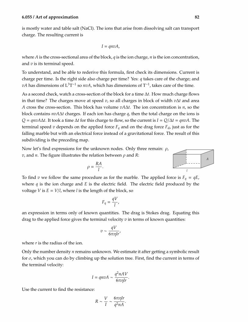
8.3.6 Conductivity of seawater

As an application of Stokes drag and a rare example of a realis­σ = 1

ρ

ρ

R = V

Iblock geometry

V = El I = qnvA

E l n v A

Fq Fd

tic situation with low Reynolds numbers, let’s estimate the elec­trical conductivity of seawater. Solving this problem is hopeless without breaking it into pieces. Conductivity σ is the reciprocal of resistivity ρ. (Apologies for the convention that overloads the density symbol with yet another meaning.) Resistivity, as its name suggests, is related to resistance R. Why have both ρ and R? Re­sistance is a useful measure for a particular wire, but not for wires in general because it depends on the diameter and cross-sectional area of the wire. It is not an intensive quantity. Before examin­ing the relationship between resistivity and resistance, let’s finish sketching the solution tree, leaving ρ as depending on R plus geometry. We can find R by placing a voltage V across a block of seawater and measuring the current I; then R = V/I.

To find V or I we need a physical model. First, why does seawater conduct at all? Con­duction requires the transport of charge, which is produced by an electric field. Seawater

82 82

82 822008-01-14 22:31:34 / rev 55add9943bf1

6.055 / Art of approximation 82

is mostly water and table salt (NaCl). The ions that arise from dissolving salt can transport charge. The resulting current is

I = qnvA,

where A is the cross-sectional area of the block, q is the ion charge, n is the ion concentration, and v is its terminal speed.

To understand, and be able to rederive this formula, first check its dimensions. Current is charge per time. Is the right side also charge per time? Yes: q takes care of the charge; and vA has dimensions of L3T−1 so nvA, which has dimensions of T−1, takes care of the time.

As a second check, watch a cross-section of the block for a time ∆t. How much charge flows in that time? The charges move at speed v, so all charges in block of width v∆t and area A cross the cross-section. This block has volume vA∆t. The ion concentration is n, so the block contains nvA∆t charges. If each ion has charge q, then the total charge on the ions is Q = qnvA∆t. It took a time ∆t for this charge to flow, so the current is I = Q/∆t = qnvA. The terminal speed v depends on the applied force Fq and on the drag force Fd, just as for the falling marble but with an electrical force instead of a gravitational force. The result of this subdividing is the preceding map.

Now let’s find expressions for the unknown nodes. Only three remain:

A

l

= qE,

ρ, v, and n. The figure illustrates the relation between ρ and R:

RA ρ = .

l

To find v we follow the same procedure as for the marble. The applied force is Fq

where q is the ion charge and E is the electric field. The electric field produced by the voltage V is E = V/l, where l is the length of the block, so

qVFq = ,

l

an expression in terms only of known quantities. The drag is Stokes drag. Equating this drag to the applied force gives the terminal velocity v in terms of known quantities:

qV ,v ∼

6πηlr

where r is the radius of the ion.

Only the number density n remains unknown. We estimate it after getting a symbolic result for σ, which you can do by climbing up the solution tree. First, find the current in terms of the terminal velocity:

q2nAV I = qnvA ∼ .

6πηlr

Use the current to find the resistance:

V 6πηlr .R ∼

I ∼

q2nA

83 83

83 832008-01-14 22:31:34 / rev 55add9943bf1

83 8 Special cases

The voltage V has vanished, which is encouraging: In most circuits the conductivity (and resistance) is independent of voltage. Use the resistance to find the resistivity:

A 6πηr ρ = R .

l ∼

q2n

The expression simplifies as we rise up the tree: The geometric parameters l and A have also vanished, which is also encouraging: The purpose of evaluating resistivity rather than resistance is that resistivity is independent of geometry.

Use resistivity to find conductivity:

1 q2n σ = ρ ∼

6πηr .

Here q is the electron charge e or its negative, depending on whether a sodium or a chloride ion is the charge carrier, so

1 e2n σ = ρ ∼

6πηr .

To find σ still requires the ion concentration n, which we can find from the concentration of salt in seawater. This value I estimate with a kitchen-sink experiment: Add table salt to a glass of water until it tastes as salty as seawater. I just tried it. In a glass of water, I found that a teaspoon of salt tastes very salty, like drinking seawater. A glass of water may have a volume of 0.3 or a mass of 300 g. A flat teaspoon of salt has a volume of about 5 m`. For those who live in metric countries, a teaspoon is an archaic measure used in Britain and especially the United States, which has no nearby metric country to which it pays attention. A teaspoon is about 4 cm long by 2 cm wide by 1 cm thick at its deepest point; let’s assume 0.5 cm on average. Its volume is therefore

teaspoon ∼ 4 cm × 2 cm × 0.5 cm ∼ 4 cm3 .

The density of salt is maybe twice the density of water, so a flat teaspoon has a mass of ∼ 10 g. The mass fraction of salt in seawater is, in this experiment, roughly 1/30. The true value is remarkably close: 0.035. A mole of salt, which provides two charges per NaCl ‘molecule’, has a mass of 60 g, so

1 2 charges 6 1023 molecules mole−1

30 × 1 g cm−3 ·

n ∼ ︸ ︷︷ ︸ ×

molecule ×

60 g mole−1

ρwater

∼ 7 1020 charges cm−3 .·

With n evaluated, the only remaining mysteries in the conductivity

1 q2n σ = ρ ∼

6πηr

are the ion radius r and the dynamic viscosity η.

Do the easy part first. The dynamic viscosity is

84 84

84 842008-01-14 22:31:34 / rev 55add9943bf1

6.055 / Art of approximation 84

η = ρwaterν ∼ 103 kg m−3 × 10−6 m2 s−1 = 10−3 kg m−1 s−1 .

Here I switched to SI (mks) units. Although most calculations are easier in cgs units – also known as God’s units – than they are in SI units, the one exception is electromagnetism, which is represented by the e2 in the conductivity. Electromagnetism is conceptually eas­ier in cgs units – which needs no ghastly µ0 or 4πε0, for example – than it is in SI units. However, the cgs unit of charge, the electrostatic unit, is unfamiliar. So, for numerical cal­culations, use SI units.

The final quantity required is the ion radius. A positive ion (sodium)

water

water

water

water

attracts an oxygen end of a water molecule; a negative ion (chloride) attracts the hydrogen end of a water molecule. Either way, the ion, being charged, is surrounded by one or maybe more layers of water molecules. As it moves, it drags some of this baggage with it. So rather than use the bare ion radius you should use a larger radius to include this shell. But how thick is the shell? As an educated guess, assume that the shell includes one layer of water molecules, each with a radius of 1.5 Å. So for the ion plus shell, r ∼ 2 Å.

With these numbers, the conductivity becomes:

2e n ︷ ︸︸ ︷ ︷ ︸︸ ︷

σ ∼ (1.6 · 10−19 C)2

×

s

7 −

· 1

1026 m

10

−3

−106 × 3 × 10−3 kg m−1 × 2 m

. ︸︷︷︸ ︸ ︷︷ ︸ ︸· ︷︷ ︸ 6π η r

You can do the computation mentally: Take out the big part, apply the principle of maximal laziness, and divide and conquer by first counting the powers of ten (shown in red) and then worrying about the small factors. Then divide and conquer again by counting the top and bottom contributions separately. The top contributes -12 powers of ten: −38 from e2 and +26 from n. The bottom contributes -13 powers of ten: −3 from η and −10 from r. The division produces one power of ten.

Now account for the remaining small factors:

1.62 × 7 .

6 × 3 × 2

Slightly overestimate the answer by pretending that the 1.62 on top cancels the 3 on the bottom. Slightly underestimate the answer – and maybe compensate for the overestimate – by pretending that the 7 on top cancels the 6 on the bottom. After these lies, only 1/2 remains. Multiplying it by the sole power of ten gives

σ ∼ 5 Ω−1 m−1 .

Using a calculator to do the arithmetic gives 4.977 . . . Ω−1 m−1, which is extremely close to the result from mental calculation.

85 85

85 852008-01-14 22:31:34 / rev 55add9943bf1

8 Special cases 85

The estimated resistivity is

ρ ∼ σ−1 ∼ 0.2 Ω m = 20 Ω cm,

where we converted to the conventional although not fully SI units of Ω cm. A typical experimental value for seawater at T = 15 C is 23.3 Ω cm (from [15, p. 14-15]), absurdly close to the estimate!

Probably the most significant error is the radius of the ion-plus-water combination that is doing the charge transport. Perhaps r should be greater than 2 Å, especially for a sodium ion, which is smaller than chloride; it therefore has a higher electric field at its surface and grabs water molecules more strongly than chloride does. In spite of such uncertainties, the continuum approximation produced more accurate results than it ought to.

At the length scale of a sodium ion, water looks like a collection of spongy boulders more than it looks like a continuum. Yet Stokes drag worked. It works because the important length scale is not the size of water molecules, but rather their mean free path between collisions. Molecules in a liquid are packed to the point of contact, so the mean free path is much shorter than a molecular (or even ionic) radius, especially compared to an ion with its shell of water.

The moral of this example, besides illustrating Stokes drag, is to have courage. Approxi­mate first and ask questions later. Maybe the approximations are correct for reasons that you do not suspect when you start solving a problem. If you agonize over each approxima­tion, you will never start a calculation, and then you will not find out that many approxi­mations would have been fine. . .if only you had had the courage to make them.

8.3.7 Turbulent limit

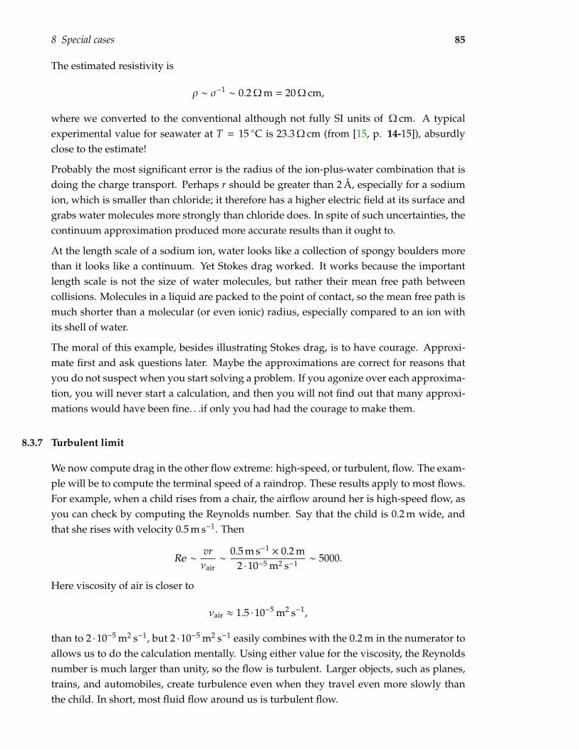
We now compute drag in the other flow extreme: high-speed, or turbulent, flow. The exam­ple will be to compute the terminal speed of a raindrop. These results apply to most flows. For example, when a child rises from a chair, the airflow around her is high-speed flow, as you can check by computing the Reynolds number. Say that the child is 0.2 m wide, and that she rises with velocity 0.5 m s−1. Then

vr 0.5 m s−1 × 0.2 m

Re ∼ νair ∼

2 10−5 m2 s−1 ∼ 5000.

·

Here viscosity of air is closer to

νair ≈ 1.5 10−5 m2 s−1 ,·

than to 2 10−5 m2 s−1, but 2 10−5 m2 s−1 easily combines with the 0.2 m in the numerator to · ·

allows us to do the calculation mentally. Using either value for the viscosity, the Reynolds number is much larger than unity, so the flow is turbulent. Larger objects, such as planes, trains, and automobiles, create turbulence even when they travel even more slowly than the child. In short, most fluid flow around us is turbulent flow.

86 86

86 862008-01-14 22:31:34 / rev 55add9943bf1

6.055 / Art of approximation 86

To begin the analysis, we assume that a raindrop is a sphere. It is a convenient lie that allows us to reuse the general results of Section 8.3.3 and specialize to high-speed flow. At high speeds (more precisely, at high Reynolds number) the flow is turbulent. Viscosity – which affects only slow flows but does not directly influence the shearing and whirling of turbulent flows – becomes irrelevant. Let’s see how much we can understand about turbulent drag knowing only that turbulent drag is nearly independent of viscosity.

Turbulence is perhaps the main unsolved problem in classical physics. However, you can still understand a lot about drag using dimensional analysis plus a bit of physical reason­ing; we do not need a full understanding of turbulence. The world is messy: Do not wait for a full understanding before you analyze or estimate.

In the roadmap for low Reynolds number, the viscosity ap- Var Dim What pears only in the first group. Because turbulent drag is in- Fd MLT−2 drag force dependent of the viscosity, the viscosity disappears from ρfl ML−3 fluid density the results and therefore so does that group. This argu­ r L object radius ment is glib. More precisely, remove ν from the list of vari­ v LT−1 terminal velocity ables and search again for dimensionless groups. The re­maining four variables, shown in the table, result in one dimensionless group, which is the second group from the old roadmap.

So the Reynolds number, which was the first group, has disappeared from the analysis. But why is drag at high speeds independent of Reynolds number? Equivalently, why can we remove ν from the list of variables and still get the correct form for the drag force? The answer is not obvious. The explanation of the Reynolds number as a ratio of two speeds v and V provides a partial answer. A natural length in this problem is r; we can use r to transform v and V into times:

r ,τv ≡

v 2r r.τV ≡

V ∼ ν

Note that Re ≡ τV/τv. The quantity τv is the time that fluid takes to travel around the sphere (apart from constants). Kinematic viscosity is ν/ρ, but its most important interpretation is as the diffusion coefficient for momentum. So the time for momentum to diffuse a distance x is

2x.τ ∼ ν

This result depends on the mathematics of random walks; you can increase your confidence in it here, without understanding the theory of random walks, by checking that it has valid dimensions. And it has: Each side is a time.

So τV is the time that momentum takes to diffuse around an object of size r, such as the falling sphere in this problem. If τV τv – in which case Re 1 – then momentum diffuses before fluid travels around the sphere. Momentum diffusion equalizes velocities, if it has time, which it does have in this low-Reynolds-number limit. Momentum diffusion

87 87

87 872008-01-14 22:31:34 / rev 55add9943bf1

8 Special cases 87

therefore prevents flow at the front from being radically different from the flow at the back, and thereby squelches any turbulence. In the other limit, when τV τv or Re 1 – momentum diffusion is outraced by fluid flow, so the fluid is free to shred itself into a turbulent mess. Once the viscosity is low enough to allow turbulence, its value does not affect the drag, which is why we can ignore it for Re 1. Here Re 1 means ‘large enough so that turbulence sets in’, which happens around Re ∼ 1000. A more complete story, which we discuss as part of boundary layers in Section 9.4, slightly corrects this approximation. However, it is close enough for our purposes here.

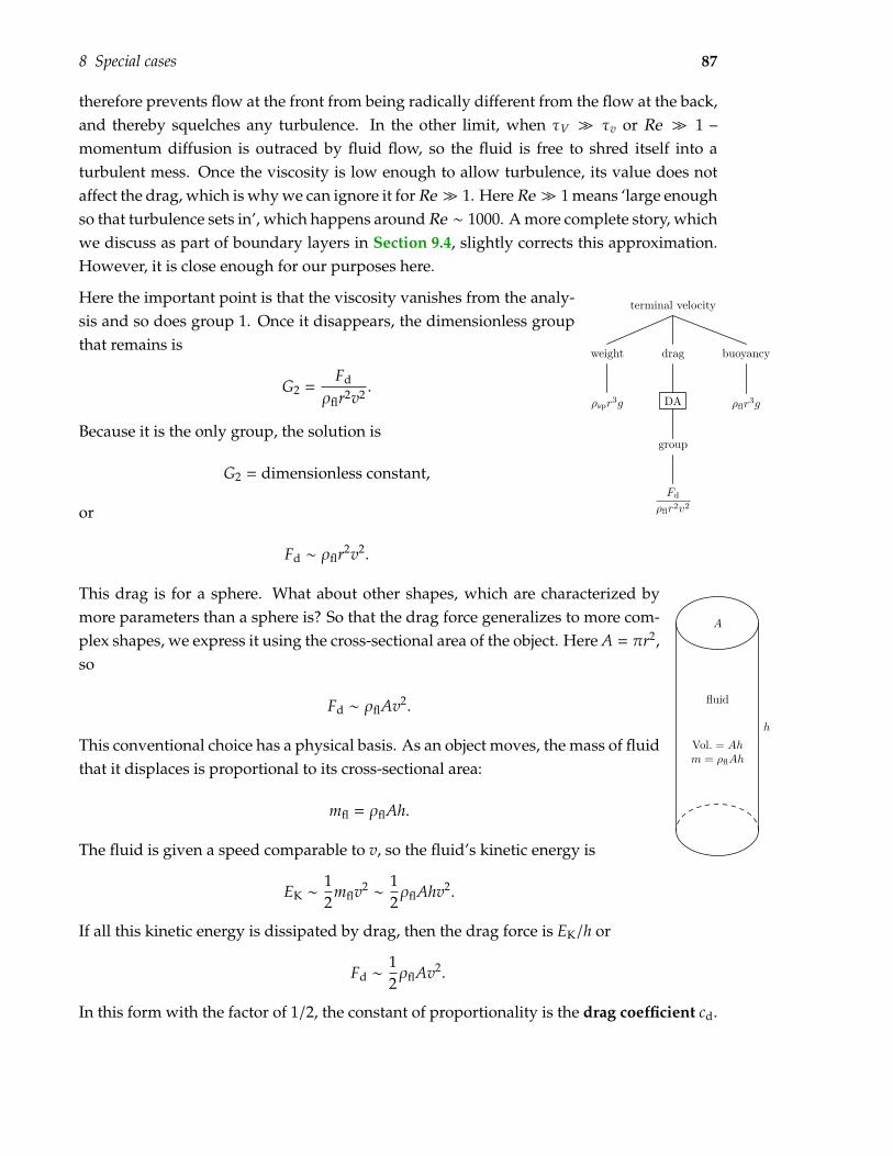
Here the important point is that the viscosity vanishes from the analy­sis and so does group 1. Once it disappears, the dimensionless group that remains is

FdG2 = ρflr2v2 .

Because it is the only group, the solution is

G2 = dimensionless constant,

or

Fd ∼ ρflr2v2 .

This drag is for a sphere. What about other shapes, which are characterized by more parameters than a sphere is? So that the drag force generalizes to more com­plex shapes, we express it using the cross-sectional area of the object. Here A 2, so

Fd ∼ ρflAv2 .

This conventional choice has a physical basis. As an object moves, the mass of fluid that it displaces is proportional to its cross-sectional area:

mfl = ρflAh.

The fluid is given a speed comparable to v, so the fluid’s kinetic energy is

EK ∼ 12

mflv2 ∼

12ρflAhv2 .

If all this kinetic energy is dissipated by drag, then the drag force is EK/h or

Fd ∼ 1 ρflAv2 .

2

In this form with the factor of 1/2, the constant of proportionality is the drag coefficient cd.

terminal velocity

weight drag buoyancy

ρspr3g ρflr3gDA

group

Fd

ρflr2v2

h

A

fluid

Vol. = Ahm = ρflAh

= πr

88 88

88 882008-01-14 22:31:34 / rev 55add9943bf1

√ ( )

6.055 / Art of approximation 88

Like its close cousin f from the dimensionless drag force, the drag coefficient Object is a dimensionless measure of the drag force. It depends on the shape of the Sphere object – on how streamlined it is. The table lists cd for various shapes (at high Cylinder Reynolds number). The drag coefficient, being proportional to the function Flat plate f (Re) in the general solution, also depends on the Reynolds number. How- Car ever, using the reasoning that the flow at high Reynolds number is indepen­dent of viscosity, the drag coefficient should also be independent of Reynolds number. Using the drag coefficient instead of f (which implies using cross-sectional area instead of r2), the turbulent drag force becomes

Fd = 1

cdρflv2A.2

So we have an expression for the turbulent drag force. The weight and buoyant forces are the same as in the viscous limit. So we just need to redo the analysis of the viscous limit but with the new drag force. Because the weight and buoyant forces contain r3, we return to using r2 instead of A in the drag force. With these results, the terminal velocity v is given by

ρflr2v2 ∼ g(ρobj − ρfl)r3 , ︸︷︷︸ ︸ ︷︷ ︸

Fd Fg−Fb

so

ρobjgr .v ∼ ρfl − 1

Pause to sanity check this result: Are the right variables upstairs and downstairs? We consider each variable in turn.

ρfl: The terminal velocity is smaller in a denser fluid (try running in a swimming pool), •

so ρfl should be in the denominator.

g: Imagine a person falling on a planet that has a gravitational force stronger than that of •

the earth. Gravity partially determines atmospheric pressure and density. Holding the atmospheric density constant while increasing gravity might be impossible in real life, but we can do it easily in a thought experiment. The drag force then does not depend on g, so gravity increases the terminal speed without opposition from the drag force: g should be upstairs.

ρobj: Imagine a raindrop made of (very) heavy water. Relative to a standard raindrop, •

the gravitational force increases while the drag force remains constant, as shown using the fluid-is-a-computer argument in ??sec:drag-force-DA. So ρobj should be upstairs.

r: To determine where the radius lives requires a more subtle argument. Increasing r•

increases both the gravitational and drag forces. The gravitational force increases as r3

cd

0.5 1.0 2.0 0.4

89 89

89 892008-01-14 22:31:34 / rev 55add9943bf1

︷ ︸︸ ︷

( ) ( )

8 Special cases 89

whereas the drag force increases only as r2. So, for larger raindrops, their greater weight increases v more than their greater drag decreases v. Therefore r should be live upstairs.

• ν: At high Reynolds number viscosity does not affect drag, at least not in our approxi­mation. So ν should not appear anywhere.

The terminal velocity passes all tests.

Now we can compute the terminal velocity. The splash spots on the sidewalk made by raindrops in a recent rain have r ∼ 0.3 cm. Since rain is water, its density is ρobj ∼ 1 g cm−3. The density of air is ρfl ∼ 1 kg m−3, so ρfl ρobj: Buoyancy is therefore not an important effect, and we can replace ρobj/ρfl − 1 by ρobj/ρfl. With this simplification and the estimated numbers, the terminal velocity is:

ρobj 1/2 1 g cm−3 v ∼ 1000 cm s−2 × 0.3 cm ×

10−3 g cm−3 ∼ 5 m s−1 ︸ ︷︷ ︸ ︸︷︷︸ ,

g r ︸ ︷︷ ︸ ρfl

or 10 mph.

This calculation assumed that Re 1. Check that assumption! You need not calculate Re from scratch; rather, scale it relative to a previous results. As we worked out earlier, a child (r ∼ 0.2 m) rising from her chair (v ∼ 0.5 m s−1) creates a turbulent flow with Re ∼ 5000. The flow created by the raindrop is faster by a factor of 10, but the raindrop is smaller by a factor of roughly 100. Scaling the Reynolds number for the child gives

Re ∼ Rechild vdrop rdrop

∼ 500. ︸ ︷︷ ︸ ×

vchild ×

rchild ︸ ︷︷ ︸ ︸ ︷︷ ︸5000 10 0.01

This Reynolds number is also much larger than 1, so the flow produced by the raindrop is turbulent, which vindicates the initial assumption.

Now that we have found the terminal velocity, let’s extract the pat­

Re 1

Re ∼ vR

ν

Fd ∼ ρv2R2

v ∼√

gRρobj

ρfl

1

3

4 2

Assume Derive

CalculateCheck

tern of the solution. The order that we followed was assume, derive, calculate, then check. This order is more fruitful than is the sim­pler order of derive then calculate. Without knowing whether the flow is fast or slow, we cannot derive a closed-form expression for Fd; such a derivation is probably beyond present understanding of fluids and turbulence. Blocked by this mathematical Everest, we would remain trapped in the derive box. We would never deter­mine Fd, so we would never realize that the Reynolds number is large (the assume box); however, only this assumption makes it possible to eliminate ν and thereby to estimate Fd. The moral: Assume early and often!

90 90

90 902008-01-14 22:31:34 / rev 55add9943bf1

( )︸︷︷︸ ︸ ︷︷ ︸

6.055 / Art of approximation 90

8.3.8 Combining solutions from the two limits

You know know the drag force in two extreme cases, viscous and turbulent drag. results are repeated here:

The

6πρflνvr (viscous),Fd = 1

2 cdρflAv2 (turbulent).

Let’s compare and combine them by making the viscous form look like the turbulent form. Compared to the turbulent form, the viscous form lacks one power of r and one power of v but has an extra power of ν. A combination of variables with a similar property is the Reynolds number rv/ν. So multiply the viscous drag by a useful form of unity:

1rv/ν6πρflv2 2r (viscous).Fd × 6πρflvρflνr= =

Re ReFd1

This form, except for the 6π and the r2, resembles the turbulent drag Fortunately A = πr2

so

Fd = 6 ρflv2A (viscous),

Re

With

12 cd = (viscous),

Re

the turbulent drag and this rewritten viscous drag for a sphere have the same form:

12 (Re 1),

Re1= ρflAv2

2Fd ×

0.5

At high Reynolds number the drag coefficient remains

(Re 1).

12Re

0.5

0.01 1 100 104

1

10

100

1000

Re

cd

If theconstant. For a sphere, that constant is cd ∼ 1/2. low-Reynolds-number approximation for cd is valid at sufficiently high Reynolds numbers, then cd would cross 1/2 near Re ∼ 24, where presumably the high-Reynolds­number approximation takes over. The crossing point is a reasonable estimate for the transition between low-and high-speed flow. Experiment or massive simulation are the only ways to get a more accurate result. Exper­imental data place the crossover near Re ∼ 5, at which point cd ∼ 2. Why can’t you calculate this value analyt­ically? If a dimensionless variable, such as the Reynolds number, is close to unity, calcu­lations become difficult. Approximations that depend on a quantity being either huge or tiny are no longer valid. When all terms in an equation are roughly of the same magnitude, you cannot get rid of any term without making large errors. To get results in these situa­tions, you have to do honest work: You must do experiments or solve the Navier–Stokes equations numerically.