600 IEEE TRANSACTIONS ON KNOWLEDGE AND DATA … · Learning Semi-Riemannian Metrics for...

Learning Semi-Riemannian Metricsfor Semisupervised Feature ExtractionWei Zhang, Zhouchen Lin, Senior Member, IEEE, and Xiaoou Tang, Fellow, IEEE

Abstract—Discriminant feature extraction plays a central role in pattern recognition and classification. Linear Discriminant Analysis

(LDA) is a traditional algorithm for supervised feature extraction. Recently, unlabeled data have been utilized to improve LDA.

However, the intrinsic problems of LDA still exist and only the similarity among the unlabeled data is utilized. In this paper, we propose

a novel algorithm, called Semisupervised Semi-Riemannian Metric Map (S3RMM), following the geometric framework of semi-

Riemannian manifolds. S3RMM maximizes the discrepancy of the separability and similarity measures of scatters formulated by using

semi-Riemannian metric tensors. The metric tensor of each sample is learned via semisupervised regression. Our method can also be

a general framework for proposing new semisupervised algorithms, utilizing the existing discrepancy-criterion-based algorithms. The

experiments demonstrated on faces and handwritten digits show that S3RMM is promising for semisupervised feature extraction.

Index Terms—Linear discriminant analysis, semisupervised learning, semi-Riemannian manifolds, feature extraction.

Ç

1 INTRODUCTION

DISCRIMINANT feature extraction is a central topic inpattern recognition and classification. Principal Com-

ponent Analysis (PCA) and Linear Discriminant Analysis(LDA) are two traditional algorithms for linear featureextraction [1]. As the underlying structure of data may notbe linear, some nonlinear feature extraction algorithms, e.g.,Locality Preserving Projections (LPP) [11] and LinearLaplacian Discrimination (LLD) [51], have been developed.In addition, the kernel trick [19] is also widely used to extendlinear feature extraction algorithms to nonlinear ones byperforming linear operations in a higher or even infinite-dimensional space transformed by a kernel mappingfunction. Despite the success of LDA and its variants [13],[42], [51], it has been found to have some intrinsic problems[40]: singularity of within-class scatter matrices and limitedavailable projection directions. Much work has been done todeal with these problems [7], [10], [35], [36], [37], [38], [39],[40], [41], [44]. Most of such work can be traced back to LDAand Fisher criterion, i.e., the structural analysis of classes bysimultaneously maximizing the between-class scatter andminimizing the within-class scatter via the ratio of them.

The discrepancy criterion has been developed recently as

an alternative way to avoid the intrinsic problems of LDA.

Such kind of methods include Maximum Margin Criterion

(MMC) [16], Kernel Scatter-Difference Analysis (KSDA)

[18], Stepwise Nonparametric Maximum Margin Criterion(SNMMC) [25], Local and Weighted Maximum MarginDiscriminant Analysis (LWMMDA) [33], Average Neigh-borhood Margin Maximization (ANMM) [32], and Discri-minative Locality Alignment (DLA) [46]. It has also beenfound that the Fisher criterion can be well solved byiterative discrepancy criterions [34]. Zhao et al. have foundthat the discrepancy criterion can be adapted into theframework of semi-Riemannian manifolds [50]. They devel-oped Semi-Riemannian Discriminant Analysis (SRDA)using this framework [50]. All these discrepancy-criterion-based methods are supervised methods.

In many real-world applications, labeled data are hard orexpensive to obtain. This makes it necessary to utilizeunlabeled data. Both labeled and unlabeled data cancontribute to the learning process [3], [53]. Consequently,semisupervised learning, which aims at learning from bothlabeled and unlabeled data, has been a hot topic within themachine learning community [53]. Many semisupervisedlearning methods have been proposed, e.g., TransductiveSVM (TSVM) [31], Cotraining [5], and graph-based semi-supervised learning algorithms [3], [28], [52]. Semisuper-vised dimensionality reduction has been consideredrecently, e.g., semisupervised discriminant analysis (SDA[6] and SSDA [48]). However, SDA and SSDA also sufferfrom the problems of the Fisher criterion, as a result ofwhich both of them use Tikhonov regularization to dealwith the singularity problem as in regularized discriminantanalysis [7]. In [43] a graph-based subspace semisupervisedlearning framework (SSLF) has been developed as asemisupervised extension of graph embedding [41] andseveral semisupervised algorithms, including SSLDA,SSLPP, and SSMFA, are provided. Supervised methodsbased on the discrepancy criterion have also been extendedto the semisupervised case, e.g., Semisupervised Discrimi-native Locality Alignment (SDLA) is the semisupervisedcounterpart of DLA [46]. SDA, SSLF, and SDLA only utilizethe smooth regularization on unlabeled or all data, whileSSDA adds a term to capture the similarity betweenunlabeled data points and class centers of labeled data.

600 IEEE TRANSACTIONS ON KNOWLEDGE AND DATA ENGINEERING, VOL. 23, NO. 4, APRIL 2011

. W. Zhang is with the Department of Information Engineering, The ChineseUniversity of Hong Kong, P.R. China. E-mail: [email protected].

. Z. Lin is with Visual Computing Group, Microsoft Research Asia, 5thFloor, Sigma Building, Zhichun Road 49#, Haidian District, Beijing100190, P.R. China. E-mail: [email protected].

. X. Tang is with the Department of Information Engineering, The ChineseUniversity of Hong Kong, P.R. China, and Shenzhen Institutes ofAdvanced Technology, Chinese Academy of Sciences, P.R. China.E-mail: [email protected].

Manuscript received 29 Mar. 2009; revised 25 Sept. 2009; accepted 29 Dec.2009; published online 24 Aug. 2010.Recommended for acceptance by S. Zhang.For information on obtaining reprints of this article, please send e-mail to:[email protected], and reference IEEECS Log Number TKDE-2009-03-0219.Digital Object Identifier no. 10.1109/TKDE.2010.143.

1041-4347/11/$26.00 � 2011 IEEE Published by the IEEE Computer Society

However, the smooth regularization may not be the optimalconstraints on samples. First, not all the neighbors of asample have the same label. Second, they set the size ofneighborhoods in advance, and then, there are no con-straints between two samples if they are not neighbors.Thus, the discriminant information among unlabeled data isnot well used.

In this paper, we propose a novel algorithm, Semisuper-vised Semi-Riemannian Metric Map (S3RMM), for semisu-pervised dimensionality reduction. Our algorithm consists oftwo steps: learning semi-Riemannian metrics and pursuingthe optimal low-dimensional projection. We formulate theproblem of learning semi-Riemannian metric tensors assemisupervised regression. Labeled data are used to initi-alize the regression. Then, a fast and efficient graph-basedsemisupervised learning scheme is adopted and closed-formsolutions are given. The optimal low-dimensional projectionis obtained via maximizing the total margin of all samplesencoded in semi-Riemannian metric tensors. Unlike previousmanifold-based algorithms [2], [3], [26], [49] in whichlearning the manifold structure does not use any class labels,we construct the manifold structure using the partial labels.Labeled samples can help discover the structure, so our semi-Riemannian manifolds can be more discriminative. Weutilize unlabeled data in two aspects: First, the unlabeleddata help to estimate the geodesic distances betweensamples, so that the structure of all data is captured; second,the separability and similarity criteria between all samplepoints, including labeled and unlabeled data, are considered.In addition, our method provides a new general frameworkfor semisupervised dimensionality reduction.

The rest of this paper is organized as follows: Section 2recalls basic conceptsof semi-Riemannianspaces. InSection 3,we begin with the discrepancy criterion and the semi-Riemannian geometry framework, then present our methodof learning semi-Riemannian metrics, and finally summarizethe S3RMM algorithm. Section 4 discusses its extensions andrelationships to the previous research. Section 5 shows theexperimental results on face and handwritten digit recogni-tion. Finally, we conclude this paper in Section 6.

2 SEMI-RIEMANNIAN SPACES

Semi-Riemannian manifolds were first applied to super-vised discriminant analysis by Zhao et al. [50].

A semi-Riemannian space is a generalization of aRiemannian space. The key difference between Riemannianand semi-Riemannian spaces is that in a semi-Riemannianspace the metric tensor need not be positive definite. Semi-Riemannian manifolds (also called pseudo-Riemannianmanifolds) are smooth manifolds furnished with semi-Riemannian metric tensors. The geometry of semi-Rieman-nian manifolds is called semi-Riemannian geometry. Semi-Riemannian geometry has been applied to Einstein’s generalrelativity, as a basic geometric tool of modeling space-timein physics. One may refer to [21] for more details.

The metric of a semi-Riemannian manifold NNn� is of the

form

� ¼��p�p; 0

0; ��

� �;

where ��p�p and �� are diagonal and their diagonal entriesare positive, andpþ � ¼ n.� is called the index of NNn

� . With�,the space-time interval ds2 in NNn

� can be written as

ds2 ¼ ðdxÞT�dx ¼Xpi¼1

��ði; iÞdx2i �

X�i¼1

�ði; iÞdx2i :

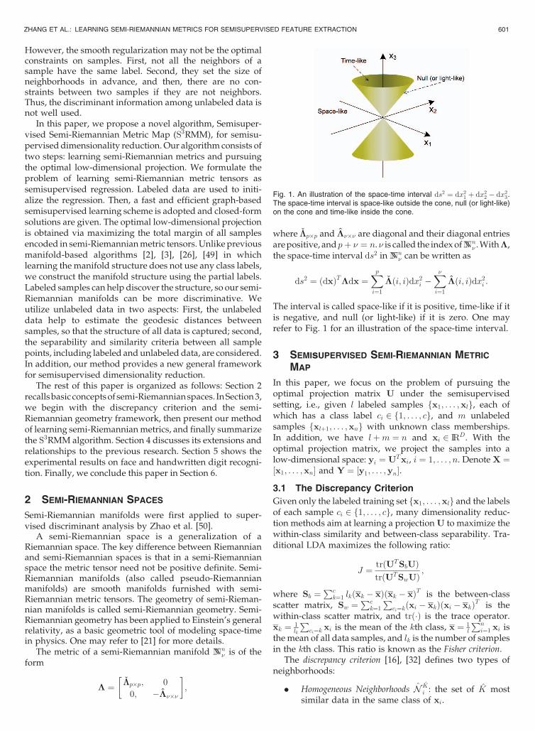
The interval is called space-like if it is positive, time-like if itis negative, and null (or light-like) if it is zero. One mayrefer to Fig. 1 for an illustration of the space-time interval.

3 SEMIsUPERVISED SEMI-RIEMANNIAN METRIC

MAP

In this paper, we focus on the problem of pursuing theoptimal projection matrix U under the semisupervisedsetting, i.e., given l labeled samples fx1; . . . ;xlg, each ofwhich has a class label ci 2 f1; . . . ; cg, and m unlabeledsamples fxlþ1; . . . ;xng with unknown class memberships.In addition, we have lþm ¼ n and xi 2 IRD. With theoptimal projection matrix, we project the samples into alow-dimensional space: yi ¼ UTxi, i ¼ 1; . . . ; n. Denote X ¼½x1; . . . ;xn� and Y ¼ ½y1; . . . ;yn�.

3.1 The Discrepancy Criterion

Given only the labeled training set fx1; . . . ;xlg and the labelsof each sample ci 2 f1; . . . ; cg, many dimensionality reduc-tion methods aim at learning a projection U to maximize thewithin-class similarity and between-class separability. Tra-ditional LDA maximizes the following ratio:

J ¼ trðUTSbUÞtrðUTSwUÞ

;

where Sb ¼Pc

k¼1 lkðxk � xÞðxk � xÞT is the between-classscatter matrix, Sw ¼

Pck¼1

Pci¼kðxi � xkÞðxi � xkÞT is the

within-class scatter matrix, and trð�Þ is the trace operator.xk ¼ 1

lk

Pci¼k xi is the mean of the kth class, x ¼ 1

l

Pni¼1 xi is

the mean of all data samples, and lk is the number of samplesin the kth class. This ratio is known as the Fisher criterion.

The discrepancy criterion [16], [32] defines two types ofneighborhoods:

. Homogeneous Neighborhoods N Ki : the set of K most

similar data in the same class of xi.

ZHANG ET AL.: LEARNING SEMI-RIEMANNIAN METRICS FOR SEMISUPERVISED FEATURE EXTRACTION 601

Fig. 1. An illustration of the space-time interval ds2 ¼ dx21 þ dx2

2 � dx23.

The space-time interval is space-like outside the cone, null (or light-like)on the cone and time-like inside the cone.

. Heterogeneous Neighborhoods �N�K

i : the set of �K mostsimilar data not in the same class of xi.

Taking ANMM [32] as an example, the average

neighborhood margin �i for xi in the projected space can

be measured as

�i ¼Xj2 �N

�K

i

1�Kkyj � yik2 �

Xj2N K

i

1

Kkyj � yik2; ð1Þ

where k � k is the L2-norm. The maximization of such a

margin can project high-dimensional data into a low-

dimensional feature space with high within-class similarity

and between-class separability. Fig. 2 gives an intuitive

illustration of the discrepancy criterion.

3.2 Semi-Riemannian-Geometry-Based FeatureExtraction Framework

The average neighborhood margin can be generalized in the

framework of semi-Riemannian geometry. In contrast to the

local semi-Riemannian metric tensors and the global align-

ment of local semi-Riemannian geometry in [50], we define

global semi-Riemannian metric tensors to unify the discre-

pancy criterion. A global metric tensor encodes the structural

relationship of all data samples to a sample, while in a local

metric tensor only samples in neighborhoods are chosen. For

a sample xi, its metric tensor �i is a diagonal matrix with

positive, negative, or zero diagonal elements:

�iðj; jÞ> 0; if xj 2 �N

�K

i ;

< 0; if xj 2 N Ki ;

¼ 0; if xj 62 �N�K

i and xj 62 N Ki :

8>><>>:Then, the construction of the homogeneous and hetero-

geneous neighborhoods as well as the metric tensor do not

need to follow those in Section 3.1.The margin �i can be written as

�i ¼Xj

�iðj; jÞkyj � yik2; ð2Þ

which is in the same form of the space-time interval. So,

we consider the sample space with class structures as a

semi-Riemannian manifold. Unlike Riemannian metric

tensors, which are positive-definite, semi-Riemannianmetric tensors can naturally encode the class structures.Thus, a semi-Riemannian manifold is more discriminative.

We define a metric matrix G, where the ith column of G(denoted as gi) is the diagonal of �i, i.e., gi ¼ ½g1i; . . . ; gni�Tand gji ¼ �iðj; jÞ (j ¼ 1; . . . ; n). An entry gji in G is called ametric component of a metric tensor gi. The projections canbe learned via maximizing the total margin

� ¼ 1

2

Xni¼1

�i ¼1

2

Xni;j¼1

gjiðyj � yiÞT ðyj � yiÞ;

¼ trðYLGYT Þ ¼ trðUTXLGXTUÞ;ð3Þ

i.e., pulling the structures of samples in the embedded low-dimensional space toward the space-likeness, where LG isthe Laplacian matrix of 1

2 ðGþGT Þ. If G is already learned(detailed in Section 3.3), the optimal linear projectionmatrix U, which projects the samples into a d-dimensionaleuclidean space and satisfies UTU ¼ Id�d and Y ¼ UTX,can be found to be composed of the eigenvectors of XLGXT

corresponding to its first d largest eigenvalues.The cases of nonlinear and multilinear embedding can be

easily extended via the kernel method and tensorization,respectively, as in [29], [32], [47].

3.3 Semisupervised Learning of Semi-RiemannianMetrics

The key problem in the semi-Riemannian geometry frame-work is to determine the metric matrix G. Under thesemisupervised setting, the metric matrix G can be dividedinto four blocks:

G ¼ GLL; GLU

GUL; GUU

� �; ð4Þ

where GLL are the metric components between labeledsamples, GLU and GUL between labeled and unlabeledsamples, and GUU between unlabeled samples. GUL, GLU ,and GUU are estimated via information propagation fromlabeled data to unlabeled data, which is a common techniquein semisupervised learning [53]. Label propagation, as a kindof information propagation, also appeared in some recentpapers on semisupervised feature extraction, e.g., [20].

In brief, the metric matrix is learned in three steps. First

of all, the metric tensors at labeled sample points, i.e., the

blocks GLL and GUL, are learned. Then, the neighborhood

relationships are propagated from metric tensors at labeled

sample points to unlabeled sample points, i.e., from GUL to

GLU . Finally, the metric tensors at unlabeled sample points,

i.e., GLU and GUU , are learned. Then, the metric tensor at a

point xi is a column vector gi of G. Similar to (4), gi can be

divided into two parts gLi and gUi , where gLi ¼ ½g1i; . . . ; gli�Tand gUi ¼ ½glþ1;i; . . . ; gni�T .

3.3.1 Local Nullity of Semi-Riemannian Manifolds

Null manifolds are a typical class of semi-Riemannianmanifolds, on which each point has a zero space-timeinterval, being neither space-like nor time-like (see Fig. 1)[21]. Inspired by the neutrality of null manifolds, we assumethat the samples in the original high-dimensional space lie ona null manifold, so that the contributions of the homogeneous


Fig. 2. An illustration of the margin maximization in the discrepancycriterion. The elements with the same shape belong to the same class.(a) xi and its neighbors in the original 2D plane, among which circlesexcept xi are homogeneous neighbors, while squares and trianglesbelong to heterogeneous neighbors. (b) yi and the projected neighbors.

and heterogeneous neighborhoods are balanced. This leadsto a local nullity condition to each metric tensor

gTi di ¼Xnj¼1

gjid2ji ¼ 0; 8i ¼ 1; . . . ; n; ð5Þ

where dji is the pairwise distance from xj to xi on the datamanifold and di ¼ ½d2

1i; . . . ; d2ni�

T .In [50] the distance dji is chosen as the known metric of the

high-dimensional feature space, e.g., the euclidean distanceand �2 distance are used for raw image features and localbinary pattern features, respectively. However, we often donot know the appropriate metrics a priori. Besides, the localstructure of samples has shown its power in unsupervisedmanifold learning [2], [26] and supervised dimensionalityreduction [11], [41], [46]. Inspired by the ISOMAP algorithm[30], we use geodesic distances, approximated by graphdistances.1 It is a great advantage of the semisupervisedsetting that a number of unlabeled data exist and can beutilized in the graph approximation of geodesic distances. So,the geodesic distances capture the manifold structure of alldata. As a result, our global semi-Riemannian metric tensorscan achieve good performance even without careful tuning ofthe sizes of the homogeneous and heterogeneous neighbor-hoods. For example in Fig. 6, it is shown that the performanceis affected very slightly when the choice of �K varies in a largerange. To testify, we use two labeled and 28 unlabeled imagesper person of 68 persons from the CMU PIE facial database(with detailed descriptions in Section 5). We comparegeodesic distances and euclidean distances in two cases:with only labeled data and with both labeled and unlabeleddata. The observations from Fig. 3 are as follows:

. According to (5), when d2ji is large, the weight of xj in

the margin of xi is suppressed. The geodesic distanceof the kth nearest neighbor increases much faster thanthe euclidean distance when k increases, so thehomogeneous and heterogeneous neighborhoods

can be selected automatically, i.e., setting K and �Kto large values has almost no influence on theperformance of our algorithm.

. With a number of unlabeled data the geodesicdistances perform better than when only labeleddata are available.

. The performance of geodesic distances is robust tothe varying parameter K, the size of neighborhoodsfor computing geodesic distances. So, we simplychoose K ¼ 5 in our implementation.

3.3.2 Metric Tensors of Labeled Samples

To determine gLi , we consider margins of labeled data first.

In ANMM [32] and DLA [46], the samples in the same kind

of neighborhood have equal weights in a margin. Such a

definition of margins only weakly models the intrinsic

structure of the training data. To overcome this drawback,

we define the average neighborhood margin normalized by

geodesic distances at a labeled point xiði ¼ 1; . . . ; lÞ as

�i ¼Xj2 �N

�K

i

1�K

kyj � yikdji

� �2

�Xj2N K

i

1

K

kyj � yikdji

� �2

; ð6Þ

where the homogeneous and heterogeneous neighborhoods

are chosen as in Section 3.1. Here, the importance of a

marginal sample xj is quantified by the distance dji to xi.

Then for xi, we have the metric components

gji ¼

1

j �N�K

i jd2ji

; if xj 2 �N�K

i ;

� 1

jN Ki jd2

ji

; if xj 2 N Ki ;

0; if xj 62 �N�K

i and xj 62 N Ki ;

8>>>>><>>>>>:ð7Þ

for all j ¼ 1; . . . ; l, where j � j is the cardinality of a set.

Equation (7) can also be obtained by the smoothness and

local nullity conditions as in [50] (please refer to the

Appendix A).Now, we come to the metric components in gUi . The

metric component gji of gi can be regarded as a function of


Fig. 3. Comparison of geodesic distances and euclidean distances. (a) only labeled data are available; (b) both labeled and unlabeled data areavailable. d2

k is the squared distance from a sample to its kth nearest neighbor. X-axis sorts the neighbors with increasing distances and the first100 neighbors are presented. Y-axis offers the ratio between minimum squared distances and d2

k. The results are averaged over 50 randomlyselected samples.

1. The geodesic distances are computed as follows: First, the K-nearest-neighbor graph is constructed for all samples and the weight of an edgeconnecting two samples is their euclidean distance. Then, the geodesicdistance between two samples is the length of the shortest path connectingthem.

xj in the sample space. So, gUi can be inferred from gLi bysemisupervised regression as follows.

We assume that nearby points are likely to have closefunction values, which is known as the smoothnessassumption. So, gji should be close to the metric compo-nents of gi corresponding to xj’s neighbors. For example, ifxj is surrounded by heterogenous neighbors of xi, gjishould be nonnegative. We choose the similarity measureajk between samples xj and xk as

ajk ¼ exp �kxj�xkk2

2�2

� �; if xj 2 NK

k or xk 2 NKj ;

0; otherwise;

(where NK

j and NKk are the K-nearest neighborhoods of xj

and xk, respectively. In our experiments, K ¼ 5 and � is theaverage distance of all sample points to their 6th nearestneighbors.

Then, we estimate the metric tensor gi by minimizing

�iðgiÞ ¼1

2

Xnj;k¼1

ajkðgji � gkiÞ2 þ �lXnj¼1

g2ji;

¼ gTi ðLA þ �lIn�nÞgi;s:t: gTi di ¼ 0 and gLi is fixed as in ð7Þ;

ð8Þ

where �l is a regularization parameter to avoid singularityof LA, which is empirically chosen as 0.01, A ¼ ½ajk�n�n, andLA is the Laplacian matrix of 1

2 ðAþAT Þ.By the Lagrangian multiplier, we get the solution of (8):

gi ¼gLigUi

" #;

gUi ¼ L�1UU

ðLULgLi ÞTL�1

UUdUi

ðdUi ÞTL�1

UUdUidUi � LULgLi

!;

ð9Þ

where the symmetric matrix ðLA þ �lIn�nÞ is divided into

LLL LLU

LUL LUU

� �similar to (4) and dUi ¼ ½d2

lþ1;i; . . . ; d2ni�

T .

3.3.3 Neighborhood Relationship Propagation

Metric tensors encode the structure of the sample space. Themetric components gji and gij are not independent becauseif xj is in the homogenous or heterogenous neighborhood ofxi, xi is probably in the same type of neighborhood of xj.So, metric tensors of labeled samples provide a prioriinformation for those of unlabeled samples. However, wedo not propagate all information in GUL as componentswith small values are disturbed more easily by noise. So, weinitialize the neighborhoods of unlabeled samples asfollows: In the metric tensor of each labeled samplexiði ¼ 1; . . . ; lÞ, we choose mK

l negative and m �Kl positive

entries from gUi with the largest absolute values, and then,put xi in the homogeneous or heterogeneous neighbor-hoods to the corresponding unlabeled samples according tothese entries’ signs. We also put the K-nearest and �K-farthest samples of an unlabeled sample in its homogeneousand heterogeneous neighborhoods, respectively, as it ismore likely for the K-nearest samples to be in the same

class as the sample and the �K-farthest samples to be in

different classes from the sample.

3.3.4 Metric Tensors of Unlabeled Samples

We initialize the metric tensor of an unlabeled sample

xi ði ¼ lþ 1; . . . ; nÞ as (7) for j ¼ 1; . . . ; n, where �N�K

i and

N Ki have been constructed in Section 3.3.3, and denote this

initial value as egi, where egi ¼ ½eg1i; . . . ; egni�T .Also by the smoothness of metric components, the metric

tensor gi can be estimated by minimizing

iðgiÞ ¼1

2

Xnj;k¼1

ajkðgji � gkiÞ2 þ �uXnj¼1

ðgji � egjiÞ2;¼ gTi ðLA þ �uIn�nÞgi � 2�uegTi gi þ �uegTi egi;

s:t: gTi di ¼ 0;

ð10Þ

where �u is a control parameter (�u > 0), which is chosen as

�u ¼ 10 in our experiments. The regularization term with

the weight �u requires that the estimated metric tensor is

not far from its initial value.By the Lagrangian multiplier, gi can be found as

gi ¼ eL�1 egi � egTi eL�1di

dTieL�1di

di

!; ð11Þ

where eL ¼ 1�u

LA þ In�n.

3.3.5 S3RMM Algorithm

The learned matrix G in the above sections is not the final

form. We shall adjust it in two steps.Noise reduction. Metric components in GUL, GLU , and

GUU are only estimations, so we need to reduce the effect of

incorrect components. Metric components close to zero are

regarded as unreliable and of little importance in a margin.

Thus, for each metric tensor gi, we set an entry gji to be zero if

xi or xj is unlabeled and jgjij < 110 maxgjigki>0jgkij. Besides, gji

and gij should reach an agreement on whether xi and xj are in

the same class. So, we split the metric matrix G to Gþ þG�,

where Gþ and G� keep the positive and negative entries of G,

respectively, while leaving the remaining entries zero. Then,

update eGþ ¼ minfGþ; ðGþÞTg and eG� ¼ maxfG�; ðG�ÞTg.Finally, we combine them with a factor � 2 ½0:5; 1�:eG ¼ ð1� �Þ eGþ þ � eG�, to make the metric tensors tend to

be time-like [50].2 � can be estimated by cross validation.Balancing contributions of labeled and unlabeled

samples. Because the target samples of classification are

only labeled samples, we suppress the contribution of

unlabeled samples as

eG0 ¼ eGLL; �1eGLU

�1eGUL; �2

eGUU

� �;

where

eG ¼ eGLLeGLUeGULeGUU

� �


2. Note that the feature extraction process pulls the initially time-likesemi-Riemannian manifold toward the space likeness.

is the metric matrix obtained after noise reduction and thevalues of �1 and �2 are chosen to be close to minf1; lmg andminf1; ð lmÞ

2g, respectively. �1 and �2 do not exceed 1 becausethe contribution of unlabeled samples should not be morethan that of labeled ones in the total margin (see (3)).

The whole procedure of S3RMM is summarized in Table 1.

4 DISCUSSION

In this section, we would like to discuss and highlight someaspects of our S3RMM algorithm.

4.1 A General Framework for SemisupervisedDimensionality Reduction

S3RMM can be viewed as a general framework forsemisupervised dimensionality reduction. First, our marginmaximization reformulation of SRDA [50] provides theconnection between the semi-Riemannian geometry frame-work and the discrepancy criterion. So, S3RMM can beintegrated with any dimensionality reduction algorithmbased on the discrepancy criterion, e.g., MMC [16], ANMM[32], and DLA [46], to obtain semisupervised extensions ofthem. To create new algorithms, we only need to change thestructural properties of semi-Riemannian metric tensors, i.e.,the constraints in (5) and (7). Second, in this framework weutilize the separability and similarity between samplesincluding labeled and unlabeled ones, instead of theregularization term on the graph of unlabeled or all samplesused in SDA [6], SSLF [43], and SDLA [46]. The traditionalregularization term is considered as a special case under ourframework (please refer to Appendix B). Finally, we onlyuse a simple yet efficient way to learn semi-Riemannianmetrics in this paper, and our method may be incorporatedwith a number of semisupervised regression methods [53].

4.2 Comparison to SRDA

The major differences between our method and SRDA [50]are threefold: First, we define global semi-Riemannianmetric tensors rather than local metric tensors as in SRDA.Second, in SRDA asymmetric semi-Riemannian metrics arelearned locally at each sample xi independently, supervisedby the label information. The relationship among themetrics at different data samples is not considered. Incontrast, in our method we learn asymmetric metrics from

labeled examples, local consistency in metric tensors andweak propagation between metric tensors globally. Third,different from the euclidean/�2 distances assumed knownin SRDA, we use geodesic distances from unsupervised

manifold learning, which do not require any a prioriknowledge of the sample space, to capture the manifoldstructure of data.

4.3 Advantages over Semisupervised DiscriminantAnalysis

S3RMM has several advantages over semisupervised dis-criminant analysis (SDA [6] and SSDA [48]). First of all, ouralgorithm can be applied to semisupervised dimensionalityreduction with pairwise constraints directly, i.e., we onlyneed to know pairwise constraints on partial samples, forlearning semi-Riemannian metrics. A pairwise constraintbetween two samples, another kind of supervision informa-tion usually used in semisupervised dimensionality reduc-tion [12], [45], describes whether they belong to the sameclass or not, rather than provides the labels. It might be tooexpensive to obtain explicit class memberships in manyreal-world applications. For example, in image retrieval it ismuch easier to know the relevance relationship betweenimages, with the logs of user relevance feedback, whileobtaining the exact class label of images requires quiteexpensive efforts of image annotation. Second, it is easy tosee that S3RMM avoids the intrinsic problems of LDA [40]:the singularity problem and limited available projectiondimensions. SDA and SSDA alleviate, but not resolve, theseproblems, as their optimization models are in the form of

J ¼ trðUTSbUÞtrðUTSwUÞ þRðUÞ

;

where RðUÞ is some regularization term on the unlabeleddata [6], [48]. In contrast, S3RMM avoids the singularityproblem, as there is no matrix inversion involved. Thenumber of possible projection dimensions in S3RMM is notlimited to ðc� 1Þ either because this limitation of LDAresults from the limited ranks of the scatter matrices.

4.4 Connection to Indefinite Kernel PCA

The maximization of the total margin in (3), after learningthe metric matrix G, aims at finding the optimal linear


TABLE 1S3RMM Algorithm

projection matrix U satisfying that Y ¼ UTX. The manifoldlearning counterpart of (3) is

maxY

tr�YLGYT

;

which is equivalent to kernel PCA using ð�LGÞy (i.e.,, thepseudo inverse of the matrix �LG) as the kernel matrix [8].From this view, learning the semi-Riemannian metricmatrix can be interpreted as indefinite kernel learning[22]. However, there are significant differences betweenS3RMM and indefinite kernel learning. First, learning themetric matrix is different from the existing indefinite kernellearning approaches, such as [15]. Our algorithm learns asparse metric matrix, while does not learn the correspondingnonsparse kernel matrix. Second, we aim at proposing alinear feature extraction method, which is not so computa-tionally expensive as kernel feature extraction and does nothave the out-of-sample problem [4]. Third, our semi-Riemannian metric matrix encodes the structural relation-ship of all data samples, but the kernel matrix is derivedfrom the mapping from the original sample space to someinfinite-dimensional Krein space [22]. Interested readersmay refer to [9], [14], [22] for the theory of Krein spaces.Finally, the existing feature extraction methods based onindefinite kernels define the kernel a priori [23]. To the bestof our knowledge, there are no feature extraction methodsutilizing indefinite kernel learning.

5 EXPERIMENTS

We compare our method to several recently proposedsemisupervised dimensionality reduction methods: SDA[6], SSDA [48], SSLDA [43], and SDLA [46]. The first threeare different semisupervised extensions of LDA and the lastone is a discrepancy-criterion-based method. We also listthe results of traditional unsupervised and supervisedalgorithms, including PCA, LDA, LPP [11], MFA [41], andMMC [16], for reference.3 Results of DLA [46] and SRDA[50] are presented for comparisons of supervised andsemisupervised methods. Note that like S3RMM, DLA/SDLA [46] also utilizes the nonlinear structure of the samplespace and extracts linear projections. We test the perfor-mance of S3RMM on two benchmark facial databases (CMUPIE and FRGC 2.0) and the USPS handwritten digit data set.

Before the experiments on real imagery data, we conductsimulations on synthetic data to show how well S3RMMworks.

5.1 Toy Experiments

To test our algorithm, we generate two kinds of 2D toy datasets: two-line data shown in Fig. 4a and two-half-circle datashown in Fig. 4b. The sample points are uniformly sampledand perturbed by random Gaussian noise. The two classes oflabeled samples are shown with circles and crosses,respectively, and the unlabeled samples are shown withpoints. We present the results of SDLA and S3RMM, asSDLA and S3RMM are both discrepancy-criterion-basedmethods with different regularization terms on the un-labeled data. SDLA adopts the graph-based regularization,

which only utilizes similarities between neighboring sam-ples, while S3RMM takes advantage of both similarities anddissimilarities between all samples, which are encoded inmetric tensors. To show how the unlabeled data affect theprojection direction, we set the weight of the term related tothe unlabeled data to be sufficiently large, and we also givethe result of DLA (i.e., the weight of the unlabeled data inSDLA is set to be zero). The classification boundary,perpendicular to the projection direction, is shown insteadfor each method, to give a more clear illustration. From Fig. 4,we can see that the graph-based regularization on theunlabeled data in SDLA works well for two-line data, anddoes not change the projection direction much for two-half-circle data. It is because for two-line data the similarities ofneighboring samples vary a lot, when we choose differentprojection directions, and for two-half-circle data they varylittle. However, S3RMM gives a nearly ideal boundarybetween the two manifolds in both data.

We also test the robustness of our algorithm to noise onthe toy data. We repeat the above experiments 20 times andfind that the correlation between projection directions inany two experiments is larger than 0.99. This result verifiesthat our algorithm is robust to noisy data.


3. We use implementations of PCA, LDA, LPP, MFA, and SDA fromhttp://www.zjucadcg.cn/dengcai/Data/data.html.

Fig. 4. Results of 2D toy experiments on two kinds of toy data.(a) Simulation results on two-line data; (b) simulation results on two-half-circle data.

5.2 Setup of Experiments on Real Data

In each experiment, we randomly select lþm images of eachperson for the training set. Then, among the lþm images,l images are randomly selected and labeled, forming thelabeled set, and the other m images form the unlabeled set.The remaining images in the database are used for testing. Wetest 50 trials of random splits and report the averaged results.

For unsupervised and supervised methods, the labeledset is used for training. For semisupervised methods, theunlabeled set is added to the training set. In all result tables,we use US, S, SS as short for Unsupervised, Supervised, andSemisupervised, respectively. A simple nearest-neighborclassifier is employed on the extracted low-dimensionalfeatures to classify samples in the unlabeled and test set.The result of the nearest-neighbor classifier on raw featureswithout dimensionality reduction is used as the baseline.

All parameters of the involved methods are tuned on thetraining set, by the full search over a relatively wide rangewhich is discretized by some step-size, e.g., for PCApreprocessing, we test with the preserved energy beingbetween 90 percent and 100 percent.

5.3 Face Recognition

In our experiments, two benchmark face databases, CMUPIE [27], and experiment 4 in FRGC 2.0 [24], are used. TheCMU PIE database contains more than 40,000 facial imagesof 68 people. The images were acquired in different poses,under various illumination conditions and with differentfacial expressions. In our experiments, a subset, the frontalpose (C 27) with varying lighting and illumination, isused. So, each person has about 49 images and in total3;329 images are collected. All the images are aligned byfixing the locations of eyes, and then, normalized to 32�32 pixels (Fig. 5a). The training set of experiment 4 inFRGC 2.0 consists of controlled and uncontrolled stillimages. We search all images of each person in this set andtake the first 60 images of the first 50 individuals thenumber of whose facial images is more than 60. Thus, wecollect 3,000 facial images for our experiments. All theimages are aligned according to the positions of eyes andmouths, and then, cropped to a size of 36� 32 (Fig. 5b).

In the first experiment, l ¼ 2, m ¼ 28, the number of testimages per individual is about 19, and the number ofindividuals is 68. In the second experiment, l ¼ 5, m ¼ 35,the number of test images per person is 20, and the numberof persons is 50. Table 2 provides results of each method.The unsupervised method, PCA, only performs a littlebetter than the baseline without any feature extraction.LDA, LPP, and MFA have good performance on PCAfeatures and SRDA, as reported in [50], outperforms thesupervised Fisher-criterion-based methods even if it is

applied to the raw data directly. The recognition results ofsemisupervised methods are generally better than theircorresponding supervised methods as they utilize theunlabeled data. S3RMM is the best in the semisupervisedmethods and improves the results of SRDA. Besides, theimprovement of S3RMM is more than the differencesbetween other methods and their supervised counterparts.4

It is interesting to know the sensitivity to the sizes ofhomogenous and heterogenous neighborhoods as ourmethod is based on maximizing the margins of suchneighborhoods. The size of homogenous neighborhoods islimited by the number of samples per class, while the size ofheterogenous neighborhoods can be much larger, as thenumber of samples not in the same class of a sample is verylarge. Because there are many possible choices of the size ofheterogenous neighborhoods, we test the robustness of ourmethod when this size changes, although the robustnessmay be implied by the properties of geodesic distancesdiscussed in Section 3.3.1. In the test, all parameters except�K are fixed. Fig. 6 shows the error rates on unlabeled and

test data of both databases with a varying number of initialheterogenous neighbors. We see here that S3RMM issurprisingly robust.

We also test the sensitivity to �l in (8) and �u in (10). Allparameters except the tested parameter (�l or �u) are fixed.Fig. 7 shows the error rates on unlabeled and test data ofboth databases with a varying value of the tested para-meter. We see that S3RMM is also robust against thevariance of these parameters in a large range.

5.4 Handwritten Digit Classification

The USPS data set contains grayscale handwritten digitimages scanned from envelopes by the US Postal Service(Fig. 8). The images are of size 16� 16. The originaltraining set contains 7,291 images, and the test set contains2,007 images.5 We used digits 1, 2, 3, 4, and 5 in ourexperiments as the five classes.

On the USPS data set we choose l ¼ 5, m ¼ 95, thenumber of test samples per class as 1,000 and the number ofclasses as 5, respectively. The classification results are listedin Table 3. PCA is only better than the baseline. The Fisher-criterion-based methods, LDA, LPP, MFA, and SSLDA, donot improve PCA features much. The discrepancy-criterion-based methods, MMC, DLA, and SRDA, are better thanother supervised methods. Unlabeled data can improve theclassification accuracy and S3RMM is the best again.

6 CONCLUSION

In this paper, we address the problem of semisupervisedfeature extraction via the semi-Riemannian geometryframework. Under this framework, the margins of samplesin the high-dimensional space are encoded in the metrictensors. We explicitly model the learning of semi-Rieman-nian metric tensors as a semisupervised regression. Then,the optimal projection is pursued by maximizing the


Fig. 5. Sample images from (a) CMU PIE database and (b) FRGC 2.0database.

4. PCA+LDA is compared with SSLDA because SSDLA is applied onPCA transformed subspace while SDA and SSDA use the Tikhonovregularization and are directly applied to the raw data.

5. We downloaded the set of 1,100 samples per class from http://www.cs.toronto.edu/~roweis/data.html.

margins of samples in the embedded low-dimensionalspace. Our algorithm can be a general framework forsemisupervised dimensionality reduction. Compared toprevious semisupervised methods, we utilize both theseparability and similarity criteria of labeled and unlabeled

samples. The links between our method and previousresearch are discussed. The effectiveness is tested on facerecognition and handwritten digit classification.

For future work, it would be interesting to see whetherour algorithm can be integrated into an active learning


Fig. 6. Recognition error rates of S3RMM against the variations of �K on unlabeled and test data of the CMU PIE and FRGC 2.0 databases. Thestandard deviations of error rates against the variations of �K are all less than 0.1 percent. (a) CMU PIE and (b) FRGC 2.0.

Fig. 7. Recognition error rates of S3RMM against the variations of �l and �u on unlabeled and test data of the CMU PIE, and FRGC 2.0 databases.The standard deviations of error rates against the variations of the parameters are also given (a) CMU PIE and (b) FRGC 2.0.

TABLE 2Recognition Error Rates (Percent, in Mean�Std-Dev) on the CMU PIE and FRGC 2.0 Databases

The reduced error rates of semisupervised methods over their supervised counterparts are given in brackets.

framework. Those zero entries corresponding to unlabeled

data in the metric matrix might indicate the marginal

samples of a sample. Therefore, it is possible to design a

strategy on how to select the most informative samples to

label. It is attractive to explore in this direction.

APPENDIX A

CONNECTION BETWEEN SRDA AND ANMM

In SRDA [50], by the smoothness and local nullity condition

they learn semi-Riemannian metrics as

�gi ¼�D�1

i e �K

eT�K�D�1

i e �K

; gi ¼eT�K

�Di�gi�K

D�1i eK ;

where �Di ¼ diagð½d2ji; j 2 �N

�K

i �Þ, Di ¼ diagð½d2ji; j 2 NK

i �Þ and

e �K , eK are all-one column vectors. Then, the margin in the

projected space for a sample xi can be written as

�i ¼ �KPj2 �N

�Ki

d�2ji

�0i, where

�0i ¼Xj2 �N

�K

i

1�K

kyj � yikdji

� �2

�Xj2N K

i

1

K

kyj � yikdji

� �2

: ð12Þ

The only difference between (12) and (1) is the distance

normalization, which can capture the structure of data better.

APPENDIX B

A SPECIAL CASE OF SEMIsUPERVISED

SEMI-RIEMANNIAN FRAMEWORK

In this appendix, we would like to show that the intrinsic

relationship between the conventional graph-based semi-

supervised dimensionality reduction methods, e.g., [43],

and our semisupervised semi-Riemannian framework.Let A ¼ 0 (which can be achieved by choosing a very

small �), i.e., remove the consistency constraints inside the

metric tensors, and we have GUL ¼ 0 from (8). Following

the neighborhood propagation, we only add K-nearest and�K-farthest neighbors of an unlabeled sample in its homo-

genous and heterogeneous neighborhoods, respectively.

Thus, we have

egji ¼1

�Kd2ji

; if xj 2 �N�K

i ;

� 1Kd2

ji

; if xj 2 N Ki ;

0; if xj 62 �N�K

i and xj 62 N Ki ;

8>>>><>>>>: ð13Þ

From Fig. 3 it is easy to see that

1

d2ji

xj2 �N�K

i

� 1

d2ji

xj2 �N K

i

as �N�K

i and �N K

i include �K-farthest and K-nearest neighbors,

respectively. Without loss of generality, let egj ¼ Kegj and we

rewrite eg as

egji ¼ � 1d2ji

; if xj 2 N Ki ;

0; if xj 62 N Ki ;

8<: ð14Þ

Still by A ¼ 0, we have gj ¼ egj. If K ¼ K, then xj 2 NKi ,

and thus,

gji ¼� 1kxj�xik2 ; if xj 2 NK

i ;

0; if xj 62 NKi :

(ð15Þ

This leads to the widely used regularization term

gji ¼�fðkxj � xikÞ; if xj 2 NK

i ;

0; if xj 62 NKi :

(ð16Þ

The function fð�Þ is chosen as fð�Þ ¼ 1 in SDA [6], SSLF [43],

and SDLA [46]. Another popular choice is fð�Þ ¼ e�ð�Þ2

�2 .

ACKNOWLEDGMENTS

This work was partially supported by the Research Grants

Council of the Hong Kong SAR (Project No. CUHK 416510).

The authors would like to thank the anonymous reviewers

for their comments, which substantially improved the

manuscript. The first author would also like to thank

Guangcan Liu et al. for sharing their manuscript on

unsupervised semi-Riemannian metric map [17] and Deli

Zhao for his valuable comments.

REFERENCES

[1] P.N. Belhumeur, J.P. Hespanha, and D.J. Kriegman, “Eigenfacesversus Fisherfaces: Recognition Using Class Specific LinearProjection,” IEEE Trans. Pattern Analysis and Machine Intelligence,vol. 19, no. 7, pp. 711-720, July 1997.

[2] M. Belkin and P. Niyogi, “Laplacian Eigenmaps for Dimension-ality Reduction and Data Representation,” Neural Computation,vol. 15, pp. 1373-1396, 2003.


TABLE 3Recognition Error Rates (Percent, in Mean�Std-Dev) on the

USPS Handwritten Digit Database

The reduced error rates of semisupervised methods over theirsupervised counterparts are given in brackets.

Fig. 8. Samples from the USPS data set.

[3] M. Belkin, P. Niyogi, and V. Sindhwani, “Manifold Regulariza-tion: A Geometric Framework for Learning from Labeled andUnlabeled Examples,” J. Machine Learning Research, vol. 7,pp. 2399-2434, 2006.

[4] Y. Bengio, J. Paiement, P. Vincent, O. Delalleau, N. Le Roux, andM. Ouimet, “Out-of-Sample Extensions for LLE, Isomap, MDS,Eigenmaps, and Spectral Clustering,” Advances in Neural Informa-tion Processing Systems, MIT Press, 2003.

[5] A. Blum and T. Mitchell, “Combining Labeled and UnlabeledData with Co-Training,” Proc. Workshop Computational LearningTheory (COLT), 1998.

[6] D. Cai, X. He, and J. Han, “Semi-Supervised DiscriminantAnalysis,” Proc. Int’l Conf. Computer Vision, 2007.

[7] J. Friedman, “Regularized Discriminant Analysis,” J. Am. Statis-tical Assoc., vol. 84, no. 405, pp. 165-175, 1989.

[8] J. Ham, D. Lee, S. Mika, and B. Scholkopf, “A Kernel View of theDimensionality Reduction of Manifolds,” Proc. Int’l Conf. MachineLearning, 2004.

[9] B. Hassibi, A. Sayed, and T. Kailath, “Linear Estimation in KreinSpaces-Part I: Theory,” IEEE Trans. Automatic Control, vol. 41,no. 1, pp. 18-33, Jan. 1996.

[10] T. Hastie, A. Buja, and R. Tibshirani, “Penalized DiscriminantAnalysis,” The Annals of Statistics, vol. 23, no. 1, pp. 73-102, 1995.

[11] X. He and P. Niyogi, “Locality Preserving Projections,” Advancesin Neural Information Processing Systems, MIT Press, 2003.

[12] S.C.H. Hoi, W. Liu, M.R. Lyu, and W.-Y. Ma, “Learning DistanceMetrics with Contextual Constraints for Image Retrieval,” Proc.IEEE Conf. Computer Vision and Pattern Recognition (CVPR ’06),2006.

[13] P. Howland and H. Park, “Generalizing Discriminant AnalysisUsing the Generalized Singular Value Decomposition,” IEEETrans. Pattern Analysis and Machine Intelligence, vol. 26, no. 8,pp. 995-1006, Aug. 2004.

[14] I. Iokhvidov, M. Krein, and H. Langer, Introduction to the SpectralTheory of Operators in Spaces with an Indefinite Metric. Akademie-Verlag, 1982.

[15] M. Kowalski, M. Szafranski, and L. Ralaivola, “Multiple IndefiniteKernel Learning with Mixed Norm Regularization,” Proc. Int’lConf. Machine Learning, 2009.

[16] H. Li, T. Jiang, and K. Zhang, “Efficient and Robust FeatureExtraction by Maximum Margin Criterion,” IEEE Trans. NeuralNetworks, vol. 17, no. 1, pp. 157-165, Jan. 2006.

[17] G. Liu, Z. Lin, and Y. Yu, “Learning Semi-Riemannian Manifoldsfor Unsupervised Dimensionality Reduction,” submitted toPattern Recognition.

[18] Q. Liu, X. Tang, H. Lu, and S. Ma, “Face Recognition Using KernelScatter-Difference-Based Discriminant Analysis,” IEEE Trans.Neural Networks, vol. 17, no. 4, pp. 1081-1085, July 2006.

[19] K. Muller, S. Mika, G. Ratsch, K. Tsuda, and B. Scholkopf, “AnIntroduction to Kernel-Based Learning Algorithms,” IEEE Trans.Neural Networks, vol. 12, no. 2, pp. 181-201, Mar. 2001.

[20] F. Nie, S. Xiang, Y. Jia, and C. Zhang, “Semi-SupervisedOrthogonal Discriminant Analysis via Label Propagation,” PatternRecognition, vol. 42, no. 11, pp. 2615-2627, 2009.

[21] B. O’Neill, Semi-Riemannian Geometry with Application to Relativity.Academic Press, 1983.

[22] C. Ong, X. Mary, S. Canu, and A. Smola, “Learning with Non-Positive Kernels,” Proc. Int’l Conf. Machine Learning, 2004.

[23] E. Pekalska and B. Haasdonk, “Kernel Discriminant Analysis forPositive Definite and Indefinite Kernels,” IEEE Trans. PatternAnalysis and Machine Intelligence, vol. 31, no. 6, pp. 1017-1032, June2009.

[24] P.J. Phillips, P.J. Flynn, T. Scruggs, K.W. Bowyer, J. Chang, K.Hoffman, J. Marques, J. Min, and W. Worek, “Overview of theFace Recognition Grand Challenge,” Proc. IEEE Conf. ComputerVision and Pattern Recognition (CVPR ’05), 2005.

[25] X. Qiu and L. Wu, “Face Recognition by Stepwise NonparametricMargin Maximum Criterion,” Proc. Int’l Conf. Computer Vision,2005.

[26] L.K. Saul, S.T. Roweis, and Y. Singer, “Think Globally, Fit Locally:Unsupervised Learning of Low Dimensional Manifolds,” J.Machine Learning Research, vol. 4, pp. 119-155, 2003.

[27] T. Sim, S. Baker, and M. Bsat, “The CMU Pose, Illumination, andExpression Database,” IEEE Trans. Pattern Analysis and MachineIntelligence, vol. 25, no. 12, pp. 1615-1618, Dec. 2003.

[28] V. Sindhwani, P. Niyogi, and M. Belkin, “Beyond the Point Cloud:From Transductive to Semi-Supervised Learning,” Proc. Int’l Conf.Machine Learning, 2005.

[29] Y. Song, F. Nie, C. Zhang, and S. Xiang, “A Unified Framework forSemi-Supervised Dimensionality Reduction,” Pattern Recognition,vol. 41, no. 9, pp. 2789-2799, 2008.

[30] J.B. Tenenbaum, V. de Silva, and J.C. Langford, “A GlobalGeometric Framework for Nonlinear Dimensionality Reduction,”Science, vol. 290, pp. 2319-2323, 2000.

[31] V. Vapnik, Statistical Learning Theory. John Wiley, 1998.[32] F. Wang and C. Zhang, “Feature Extraction by Maximizing the

Average Neighborhood Margin,” Proc. IEEE Conf. Computer Visionand Pattern Recognition (CVPR ’07), 2007.

[33] H. Wang, W. Zheng, Z. Hu, and S. Chen, “Local and WeightedMaximum Margin Discriminant Analysis,” Proc. IEEE Conf.Computer Vision and Pattern Recognition (CVPR ’07), 2007.

[34] H. Wang, S. Yan, D. Xu, X. Tang, and T. Huang, “Trace Ratioversus Ratio Trace for Dimensionality Reduction,” Proc. IEEEConf. Computer Vision and Pattern Recognition (CVPR ’07), 2007.

[35] X. Wang and X. Tang, “Unified Subspace Analysis for FaceRecognition,” Proc. Int’l Conf. Computer Vision, 2003.

[36] X. Wang and X. Tang, “Dual-Space Linear Discriminant Analysisfor Face Recognition,” Proc. IEEE Conf. Computer Vision and PatternRecognition (CVPR ’04), 2004.

[37] X. Wang and X. Tang, “Random Sampling LDA for FaceRecognition,” Proc. IEEE Conf. Computer Vision and PatternRecognition (CVPR ’04), 2004.

[38] X. Wang and X. Tang, “A Unified Framework for Subspace FaceRecognition,” IEEE Trans. Pattern Analysis and Machine Intelligence,vol. 26, no. 9, pp. 1222-1228, Sept. 2004.

[39] X. Wang and X. Tang, “Random Sampling for Subspace FaceRecognition,” Int’l J. Computer Vision, vol. 70, no. 1, pp. 91-104,2006.

[40] S. Yan, D. Xu, Q. Yang, L. Zhang, X. Tang, and H.-J. Zhang,“Multilinear Discriminant Analysis for Face Recognition,” IEEETrans. Image Processing, vol. 16, no. 1, pp. 212-220, Jan. 2007.

[41] S. Yan, D. Xu, B. Zhang, H.-J. Zhang, Q. Yang, and S. Lin, “GraphEmbedding and Extensions: A General Framework for Dimen-sionality Reduction,” IEEE Trans. Pattern Analysis and MachineIntelligence, vol. 29, no. 1, pp. 40-51, Jan. 2007.

[42] J. Yang, A. Frangi, J. Yang, D. Zhang, and Z. Jin, “KPCA PlusLDA: A Complete Kernel Fisher Discriminant Framework forFeature Extraction and Recognition,” IEEE Trans. Pattern Analysisand Machine Intelligence, vol. 27, no. 2, pp. 230-244, Feb. 2005.

[43] W. Yang, S. Zhang, and W. Liang, “A Graph Based SubspaceSemi-Supervised Learning Framework for Dimensionality Reduc-tion,” Proc. European Conf. Computer Vision, 2008.

[44] J. Ye, R. Janardan, and Q. Li, “Two-Dimensional LinearDiscriminant Analysis,” Advances in Neural Information ProcessingSystems, MIT Press, 2004.

[45] D. Zhang, Z.-H. Zhou, and S. Chen, “Semi-Supervised Dimen-sionality Reduction,” Proc. SIAM Int’l Conf. Data Mining, 2007.

[46] T. Zhang, D. Tao, and J. Yang, “Discriminative Locality Align-ment,” Proc. European Conf. Computer Vision, 2008.

[47] W. Zhang, Z. Lin, and X. Tang, “Tensor Linear LaplacianDiscrimination (TLLD) for Feature Extraction,” Pattern Recogni-tion, vol. 42, no. 9, pp. 1941-1948, 2009.

[48] Y. Zhang and D.-Y. Yeung, “Semi-Supervised DiscriminantAnalysis Using Robust Path-Based Similarity,” Proc. IEEE Conf.Computer Vision and Pattern Recognition, 2008.

[49] Z. Zhang and H. Zha, “Principal Manifolds and NonlinearDimensionality Reduction via Tangent Space Alignment,” SIAMJ. Scientific Computing, vol. 26, no. 1, pp. 313-338, 2005.

[50] D. Zhao, Z. Lin, and X. Tang, “Classification via Semi-RiemannianSpaces,” Proc. IEEE Conf. Computer Vision and Pattern Recognition(CVPR ’08), 2008.

[51] D. Zhao, Z. Lin, R. Xiao, and X. Tang, “Linear LaplacianDiscrimination for Feature Extraction,” Proc. IEEE Conf. ComputerVision and Pattern Recognition (CVPR ’07), 2007.

[52] D. Zhou, O. Bousquet, T.N. Lal, J. Weston, and B. Scholkopf,“Learning with Local and Global Consistency,” Advances in NeuralInformation Processing Systems, pp. 321-328, MIT Press, 2004.

[53] X. Zhu, “Semi-Supervised Learning Literature Survey,” technicalreport, Computer Science Dept., Univ. of Wisconsin-Madison,2005.


Wei Zhang received the BEng degree inelectronic engineering from the Tsinghua Uni-versity, Beijing, in 2007, and the MPhil degree ininformation engineering in 2009 from TheChinese University of Hong Kong, where he iscurrently working toward the PhD degree at theDepartment of Information Engineering. Hisresearch interests include machine learning,computer vision, and image processing.

Zhouchen Lin received the PhD degree inapplied mathematics from Peking University, in2000. He is currently a lead researcher in VisualComputing Group, Microsoft Research, Asia.His research interests include computer vision,image processing, machine learning, patternrecognition, numerical computation and optimi-zation, and computer graphics. He is a seniormember of the IEEE.

Xiaoou Tang received the BS degree from theUniversity of Science and Technology of China,Hefei, in 1990, the MS degree from theUniversity of Rochester, Rochester, New York,in 1991, and the PhD degree from the Massa-chusetts Institute of Technology, Cambridge, in1996. He is a professor in the Department ofInformation Engineering and associate dean(research) of the Faculty of Engineering at theChinese University of Hong Kong. He worked as

the group manager of the Visual Computing Group at MicrosoftResearch Asia from 2005 to 2008. His research interests includecomputer vision, pattern recognition, and video processing. He receivedthe Best Paper Award from the IEEE Conference on Computer Visionand Pattern Recognition (CVPR) in 2009. He is a program chair of theIEEE International Conference on Computer Vision (ICCV) 2009 and anassociate editor of the IEEE Transactions on Pattern Analysis andMachine Intelligence (TPAMI), and the International Journal ofComputer Vision (IJCV). He is a fellow of the IEEE.

. For more information on this or any other computing topic,please visit our Digital Library at www.computer.org/publications/dlib.


600 IEEE TRANSACTIONS ON KNOWLEDGE AND DATA … · Learning Semi-Riemannian Metrics for...

Documents

Transcript of 600 IEEE TRANSACTIONS ON KNOWLEDGE AND DATA … · Learning Semi-Riemannian Metrics for...