6 Linear Elasticity - Aucklandhomepages.engineering.auckland.ac.nz/~pkel015/... · 143 6 Linear...

143

6 Linear Elasticity The simplest constitutive law for solid materials is the linear elastic law, which assumes a linear relationship between stress and engineering strain. This assumption turns out to be an excellent predictor of the response of components which undergo small deformations, for example steel and concrete structures under large loads, and also works well for practically any material at a sufficiently small load. The linear elastic model is discussed in this chapter and some elementary problems involving elastic materials are solved. Anisotropic elasticity is discussed in Section 6.3.

Section 6.1

Solid Mechanics Part I Kelly 145

6.1 The Linear Elastic Model 6.1.1 The Linear Elastic Model Repeating some of what was said in Section 5.3: the Linear Elastic model is used to describe materials which respond as follows:

(i) the strains in the material are small1 (linear) (ii) the stress is proportional to the strain, (linear) (iii) the material returns to its original shape when the loads are removed, and the

unloading path is the same as the loading path (elastic) (iv) there is no dependence on the rate of loading or straining (elastic)

From the discussion in the previous chapter, this model well represents the engineering materials up to their elastic limit. It also models well almost any material provided the stresses are sufficiently small. The stress-strain (loading and unloading) curve for the Linear Elastic solid is shown in Fig. 6.1.1a. Other possible responses are shown in Figs. 6.1.1b,c. Fig. 6.1.1b shows the typical response of a rubbery-type material and many biological tissues; these are non-linear elastic materials. Fig. 6.1.1c shows the typical response of viscoelastic materials (see Chapter 10) and that of many plastically and viscoplastically deforming materials (see Chapters 11 and 12).

Figure 6.1.1: Different stress-strain relationships; (a) linear elastic, (b) non-linear elastic, (c) viscoelastic/plastic/viscoplastic

It will be assumed at first that the material is isotropic and homogeneous. The case of an anisotropic elastic material is discussed in Section 6.3.

1 if the small-strain approximation is not made, the stress-strain relationship will be inherently non-linear; the actual strain, Eqn. 4.1.7, involves (non-linear) squares and square-roots of lengths

load

unload

)a( )b( )c(

hysteresis loop

Section 6.1


6.1.2 Stress-Strain Law Consider a cube of material subjected to a uniaxial tensile stress xx , Fig. 6.1.2a. One

would expect it to respond by extending in the x direction, 0xx , and to contract

laterally, so 0 zzyy , these last two being equal because of the isotropy of the

material. With stress proportional to strain, one can write

xxzzyyxxxx EE ,

1 (6.1.1)

Figure 6.1.2: an element of material subjected to a uniaxial stress; (a) normal strain,

(b) shear strain The constant of proportionality between the normal stress and strain is the Young’s Modulus, Eqn. 5.2.5, the measure of the stiffness of the material. The material parameter is the Poisson’s ratio, Eqn. 5.2.6. Since xxzzyy , it is a measure of the

contraction relative to the normal extension. Because of the isotropy/symmetry of the material, the shear strains are zero, and so the deformation of Fig. 6.1.2b, which shows a non-zero xy , is not possible – shear strain can

arise if the material is not isotropic. One can write down similar expressions for the strains which result from a uniaxial tensile yy stress and a uniaxial zz stress:

zzyyxxzzzz

yyzzxxyyyy

EE

EE

,1

,1

(6.1.2)

Similar arguments can be used to write down the shear strains which result from the application of a shear stress:

xzxzyzyzxyxy

2

1,

2

1,

2

1 (6.1.3)

xx

xx

)a(

xx

xx

)b(

Section 6.1


The constant of proportionality here is the Shear Modulus , Eqn. 5.2.8, the measure of the resistance to shear deformation (the letter G was used in Eqn. 5.2.8 – both G and are used to denote the Shear Modulus, the latter in more “mathematical” and “advanced” discussions) . The strain which results from a combination of all six stresses is simply the sum of the strains which result from each2:

yyxxzzzz

yzyzzzxxyyyy

xzxzxyxyzzyyxxxx

E

E

E

1

2

1,

1

,2

1,

2

1,

1

(6.1.4)

These equations involve three material parameters. It will be proved in §6.3 that an isotropic linear elastic material can have only two independent material parameters and that, in fact,

12

E. (6.1.5)

This relation will be verified in the following example. Example: Verification of Eqn. 6.1.5 Consider the simple shear deformation shown in Fig. 6.1.3, with 0xy and all other

strains zero. With the material linear elastic, the only non-zero stress is xyxy 2 .

Figure 6.1.3: a simple shear deformation

2 this is called the principle of linear superposition: the "effect" of a sum of "causes" is equal to the sum of the individual "effects" of each "cause". For a linear relation, e.g. E , the effects of two causes

,1 2 are 1E and 2E , and the effect of the sum of the causes 1 2 is indeed equal to the sum of the

individual effects: 1 2 1 2( )E E E . This is not true of a non-linear relation, e.g. 2E , since 2 2 2

1 2 1 2( )E E E

xy

x

y

Section 6.1


Using the strain transformation equations, Eqns. 4.2.2, the only non-zero strains in a second coordinate system yx , with x at o45 from the x axis (see Fig. 6.1.3), are

xyxx and xyyy . Because the material is isotropic, Eqns 6.1.4 hold also in this

second coordinate system and so the stresses in the new coordinate system can be determined by solving the equations

yyxxzzzz

yzyzzzxxyyxyyy

xzxzxyxyzzyyxxxyxx

E

E

E

10

2

10,

1

,2

10,

2

10,

1

(6.1.6)

which results in

xyyyxyxx v

E

v

E

1

,1

(6.1.7)

But the stress transformation equations, Eqns. 3.4.8, with xyxy 2 , give

xyxx 2 and xyyy 2 and so Eqn. 6.1.5 is verified.

■ Relation 6.1.5 allows the Linear Elastic Solid stress-strain law, Eqn. 6.1.4, to be written as

yzyz

xzxz

xyxy

yyxxzzzz

zzxxyyyy

zzyyxxxx

E

E

E

E

E

E

1

1

1

1

1

1

Stress-Strain Relations (6.1.8)

This is known as Hooke’s Law. These equations can be solved for the stresses to get

Section 6.1


yzyz

xzxz

xyxy

yyxxzzzz

zzxxyyyy

zzyyxxxx

E

E

E

E

E

E

1

1

1

)1()21)(1(

)1()21)(1(

)1()21)(1(

Stress-Strain Relations (6.1.9)

Values of E and for a number of materials are given in Table 6.1.1 below (see also Table 5.2.2).

Table 6.1.1: Young’s Modulus E and Poisson’s Ratio ν for a selection of materials at

20oC Volume Change Recall that the volume change in a material undergoing small strains is given by the sum of the normal strains (see Section 4.3). From Hooke’s law, normal stresses cause normal strain and shear stresses cause shear strain. It follows that normal stresses produce volume changes and shear stresses produce distortion (change in shape), but no volume change. 6.1.3 Two Dimensional Elasticity The above three-dimensional stress-strain relations reduce in the case of a two-dimensional stress state or a two-dimensional strain state.

Material E (GPa) Grey Cast Iron 100 0.29A316 Stainless Steel 196 0.3A5 Aluminium 68 0.33Bronze 130 0.34Plexiglass 2.9 0.4Rubber 0.001-2 0.4-0.49Concrete 23-30 0.2Granite 53-60 0.27Wood (pinewood)fibre direction transverse direction

171

0.450.79

Section 6.1


Plane Stress In plane stress (see Section 3.5), 0 zzyzxz , Fig. 6.1.5, so the stress-strain

relations reduce to

xyxy

yyxxyy

yyxxxx

xyxy

xxyyyy

yyxxxx

E

E

E

E

E

E

1

1

1

1

1

1

2

2

Stress-Strain Relations (Plane Stress) (6.1.10) with

0

0,

yzxzzz

yzxzyyxxzz E

(6.1.11)

Figure 6.1.5: Plane stress Note that the zz strain is not zero. Physically, zz corresponds to a change in thickness of the material perpendicular to the direction of loading. Plane Strain In plane strain (see Section 4.2), 0 zzyzxz , Fig. 6.1.6, and the stress-strain

relations reduce to

y

xz

Section 6.1


xyxy

xxyyyy

yyxxxx

xyxy

yyxxyy

yyxxxx

E

E

E

E

E

E

1

)1()21)(1(

)1()21)(1(

1

)1(1

)1(1

Stress-Strain Relations (Plane Strain) (6.1.12) with

0,

0

yzxzyyxxzz

yzxzzz

(6.1.13)

Again, note here that the stress component zz is not zero. Physically, this stress corresponds to the forces preventing movement in the z direction.

Figure 6.1.6 Plane strain - a thick component constrained in one direction Similar Solutions The expressions for plane stress and plane strain are very similar. For example, the plane strain constitutive law 6.1.12 can be derived from the corresponding plane stress expressions 6.1.10 by making the substitutions

1

,1 2

EE (6.1.14)

in 6.1.10 and then dropping the primes. The plane stress expressions can be derived from the plane strain expressions by making the substitutions

1

,1

212

EE (6.1.15)

zz

Section 6.1


in 6.1.12 and then dropping the primes. Thus, if one solves a plane stress problem, one has automatically solved the corresponding plane strain problem, and vice versa. 6.1.4 Problems 1. A strain gauge at a certain point on the surface of a thin A5 Aluminium component

(loaded in-plane) records strains of μm15μm,30μm,60 xyyyxx .

Determine the principal stresses. (See Table 6.1.1 for the material properties.) 2. Use the stress-strain relations to prove that, for a linear elastic solid,

yyxx

xy

yyxx

xy

22

and, indeed,

zzyy

yz

zzyy

yz

zzxx

xz

zzxx

xz

22,

22

Note: from Eqns. 3.5.4 and 4.2.4, these show that the principal axes of stress and strain coincide for an isotropic elastic material

3. Consider the case of hydrostatic pressure in a linearly elastic solid:

p

p

p

ij

00

00

00

as might occur, for example, when a spherical component is surrounded by a fluid under high pressure, as illustrated in the figure below. Show that the volumetric strain (Eqn. 4.3.5) is equal to

E

p213

,

so that the Bulk Modulus, Eqn. 5.2.9, is

3 1 2

EK

4. Consider again Problem 2 from §3.5.7.

(a) Assuming the material to be linearly elastic, what are the strains? Draw a second material element (superimposed on the one shown below) to show the deformed shape of the square element – assume the displacement of the box-centre to be zero and that there is no rotation. Note how the free surface moves, even though there is no stress acting on it.

Section 6.1


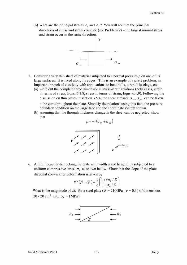
(b) What are the principal strains 1 and 2 ? You will see that the principal directions of stress and strain coincide (see Problem 2) – the largest normal stress and strain occur in the same direction.

5. Consider a very thin sheet of material subjected to a normal pressure p on one of its

large surfaces. It is fixed along its edges. This is an example of a plate problem, an important branch of elasticity with applications to boat hulls, aircraft fuselage, etc. (a) write out the complete three dimensional stress-strain relations (both cases, strain

in terms of stress, Eqns. 6.1.8, stress in terms of strain, Eqns. 6.1.9). Following the discussion on thin plates in section 3.5.4, the shear stresses yzxz , , can be taken

to be zero throughout the plate. Simplify the relations using this fact, the pressure boundary condition on the large face and the coordinate system shown.

(b) assuming that the through thickness change in the sheet can be neglected, show that

yyxxp

6. A thin linear elastic rectangular plate with width a and height b is subjected to a uniform compressive stress 0 as shown below. Show that the slope of the plate

diagonal shown after deformation is given by

0

0

1 /tan

1 /

b E

a E

What is the magnitude of for a steel plate ( GPa210E , 3.0 ) of dimensions 2cm2020 with MPa10 ?

px

y

z

00

xx

y

xx

Section 6.2


6.2 Homogeneous Problems in Linear Elasticity A homogeneous stress (strain) field is one where the stress (strain) is the same at all points in the material. Homogeneous conditions will arise when the geometry is simple and the loading is simple. 6.2.1 Elastic Rectangular Cuboids Hooke’s Law, Eqns. 6.1.8 or 6.1.9, can be used to solve problems involving homogeneous stress and deformation. Hoooke’s law is 6 equations in 12 unknowns (6 stresses and 6 strains). If some of these unknowns are given, the rest can be found from the relations. Example Consider the block of linear elastic material shown in Fig. 6.2.1. It is subjected to an equi-biaxial stress of 0 yyxx .

Since this is an isotropic elastic material, the shears stresses and strains will be all zero for such a loading. One thus need only consider the three normal stresses and strains. There are now 3 equations (the first 3 of Eqns. 6.1.8 or 6.1.9) in 6 unknowns. One thus needs to know three of the normal stresses and/or strains to find a solution. From the loading, one knows that xx and yy . The third piece of information comes

from noting that the surfaces parallel to the yx plane are free surfaces (no forces acting

on them) and so 0zz . From Eqn. 6.1.8 then, the strains are

0,2,)1( yzxzxyzzyyxx EE

As expected, yyxx and 0zz .

Figure 6.2.1: A block of linear elastic material subjected to an equi-biaxial stress

■

x

y

z

Section 6.2


6.2.2 Problems 1. A block of isotropic linear elastic material is subjected to a compressive normal stress

o over two opposing faces. The material is constrained (prevented from moving) in

one of the direction normal to these faces. The other faces are free. (a) What are the stresses and strains in the block, in terms of Eo ,, ?

(b) Calculate three maximum shear stresses, one for each plane (parallel to the faces of the block). Which of these is the overall maximum shear stress acting in the block?

2. Repeat problem 1a, only with the free faces now fixed also.

Section 6.3


6.3 Anisotropic Elasticity There are many materials which, although well modelled using the linear elastic model, are not nearly isotropic. Examples are wood, composite materials and many biological materials. The mechanical properties of these materials differ in different directions. Materials with this direction dependence are called anisotropic (see Section 5.2.7). 6.3.1 Material Constants The most general form of Hooke’s law, the generalised Hooke’s Law, for a linear elastic material is

xy

xz

yz

zz

yy

xx

xy

xz

yz

zz

yy

xx

CCCCCC

CCCCCC

CCCCCC

CCCCCC

CCCCCC

CCCCCC

6

5

4

3

2

1

666564636261

565554535251

464544434241

363534333231

262524232221

161514131211

6

5

4

3

2

1

(6.3.1)

where each stress component depends (linearly) on all strain components. This new notation, with only one subscript for the stress and strain, numbered from 1…6, is helpful as it allows the equations of anisotropic elasticity to be written in matrix form. The 36

s'ijC are material constants called the stiffnesses, and in principle are to be obtained

from experiment. The matrix of stiffnesses is called the stiffness matrix. Note that these equations imply that a normal stress xx will induce a material element to not only stretch

in the x direction and contract laterally, but to undergo shear strain too, as illustrated schematically in Fig. 6.3.1.

Figure 6.3.1: an element undergoing shear strain when subjected to a normal stress

only In section 8.4.3, when discussing the strain energy in an elastic material, it will be shown that it is necessary for the stiffness matrix to be symmetric and so there are only 21 independent elastic constants in the most general case of anisotropic elasticity. Eqns. 6.3.1 can be inverted so that the strains are given explicitly in terms of the stresses:

xxxx

Section 6.3


6

5

4

3

2

1

66

5655

464544

36353433

2625242322

161514131211

6

5

4

3

2

1

S

SS

SSS

SSSS

SSSSS

SSSSSS

(6.3.2)

The s'ijS here are called compliances, and the matrix of compliances is called the

compliance matrix. The bottom half of the compliance matrix has been omitted since it too is symmetric. It is difficult to model fully anisotropic materials due to the great number of elastic constants. Fortunately many materials which are not fully isotropic still have certain material symmetries which simplify the above equations. These material types are considered next. 6.3.2 Orthotropic Linear Elasticity An orthotropic material is one which has three orthogonal planes of microstructural symmetry. An example is shown in Fig. 6.3.2a, which shows a glass-fibre composite material. The material consists of thousands of very slender, long, glass fibres bound together in bundles with oval cross-sections. These bundles are then surrounded by a plastic binder material. The continuum model of this composite material is shown in Fig. 6.3.2b wherein the fine microstructural details of the bundles and surrounding matrix are “smeared out” and averaged. Three mutually perpendicular planes of symmetry can be passed through each point in the continuum model. The zyx ,, axes forming these planes are called the material directions.

Figure 6.3.2: an orthotropic material; (a) microstructural detail, (b) continuum model

y

z

x

y

z

x

)a( )b(

binder fibre bundles

Section 6.3


The material symmetry inherent in the orthotropic material reduces the number of independent elastic constants. To see this, consider an element of orthotropic material subjected to a shear strain xy 6 and also a strain xy 6 , as in Fig. 6.3.3.

Figure 6.3.3: an element of orthotropic material undergoing shear strain From Eqns. 6.3.1, the stresses induced by a strain 6 only are

666665656464

636362626161

,,

,,

CCC

CCC

(6.3.3)

The stresses induced by a strain 6 only are (the prime is added to distinguish these

stresses from those of Eqn. 6.3.3)

666665656464

636362626161

,,

,,

CCC

CCC

(6.3.4)

These stresses, together with the strain, are shown in Fig. 6.3.4 (the microstructure is also indicated)

Figure 6.3.4: an element of orthotropic material undergoing shear strain; (a) positive strain, (b) negative strain

Because of the symmetry of the material (print this page out, turn it over, and Fig. 6.3.4a viewed from the “other side” of the page is the same as Fig. 6.3.4b on “this side” of the page), one would expect the normal stresses in Fig. 6.3.4 to be the same, 11 ,

6

6zx

y

1

26

1

2 6

)a( )b(

Section 6.3


22 , but the shear stresses to be of opposite sign, 66 . Eqns. 6.3.3-4 then

imply that

05646362616 CCCCC (6.3.5)

Similar conclusions follow from considering shear strains in the other two planes:

0:

0:

3424144

453525155

CCC

CCCC

(6.3.6)

The stiffness matrix is thus reduced, and there are only nine independent elastic constants:

6

5

4

3

2

1

66

55

44

33

2322

131211

6

5

4

3

2

1

0

00

000

000

000

C

C

C

C

CC

CCC

(6.3.7)

These equations can be inverted to get, introducing elastic constants E, and G in place of the sSij ' :

6

5

4

3

2

1

12

13

23

32

23

1

13

3

32

21

12

3

31

2

21

1

6

5

4

3

2

1

2

100000

02

10000

002

1000

0001

0001

0001

G

G

G

EEE

EEE

EEE

(6.3.8)

The nine independent constants here have the following meanings:

iE is the Young’s modulus (stiffness) of the material in direction 3,2,1i ; for example,

111 E for uniaxial tension in the direction 1.

ij is the Poisson’s ratio representing the ratio of a transverse strain to the applied strain

in uniaxial tension; for example, 1212 / for uniaxial tension in the direction 1.

Section 6.3


ijG are the shear moduli representing the shear stiffness in the corresponding plane; for

example, 12G is the shear stiffness for shearing in the 1-2 plane. If the 1-axis has long fibres along that direction, it is usual to call 12G and 13G the axial

shear moduli and 23G the transverse (out-of-plane) shear modulus.

Note that, from symmetry of the stiffness matrix,

121212131313232323 ,, EEEEEE (6.3.9)

An important feature of the orthotropic material is that there is no shear coupling with respect to the material axes. In other words, normal stresses result in normal strains only and shear stresses result in shear strains only. Note that there will in general be shear coupling when the reference axes used, zyx ,, , are not aligned with the material directions 3,2,1 . For example, suppose that the yx axes were oriented to the material axes as shown in Fig. 6.3.5. Assuming that the material constants were known, the stresses and strains in the constitutive equations 6.3.8 can be transformed into xyxx , , etc. and xyxx , , etc. using the strain and stress

transformation equations. The resulting matrix equations relating the strains xyxx , to

the stresses xyxx , will then not contain zero entries in the stiffness matrix, and normal

stresses, e.g. xx , will induce shear strain, e.g. xy , and shear stress will induce normal

strain.

Figure 6.3.5: reference axes not aligned with the material directions 6.3.3 Transversely Isotropic Linear Elasticity A transversely isotropic material is one which has a single material direction and whose response in the plane orthogonal to this direction is isotropic. An example is shown in Fig. 6.3.6, which again shows a glass-fibre composite material with aligned fibres, only now the cross-sectional shapes of the fibres are circular. The characteristic material direction is z and the material is isotropic in any plane parallel to the yx plane. The material properties are the same in all directions transverse to the fibre direction.

x

y

12

Section 6.3


Figure 6.3.6: a transversely isotropic material This extra symmetry over that inherent in the orthotropic material reduces the number of independent elastic constants further. To see this, consider an element of transversely isotropic material subjected to a normal strain xx 1 only of magnitude , Fig.

6.3.7a, and also a normal strain yy 2 of the same magnitude, , Fig. 6.3.7b. The

yx plane is the plane of isotropy.

Figure 6.3.7: elements of a transversely isotropic material undergoing normal strain

in the plane of isotropy From Eqns. 6.3.7, the stresses induced by a strain 1 only are

0,0,0

,,

654

313212111

CCC

(6.3.10)

The stresses induced by the strain 2 only are (the prime is added to distinguish these stresses from those of Eqn. 6.3.10)

0,0,0

,,

654

323222121

CCC

(6.3.11)

Because of the isotropy, the )(1 xx due to the 1 should be the same as the

)(2 yy due to the 2 , and it follows that 2211 CC . Further, the )(3 zz should

be the same for both, and so 3231 CC .

y

z

x

x

y

x

y

)a( )b(

Section 6.3


Further simplifications arise from consideration of shear deformations, and rotations about the material axis, and one finds that 5544 CC and 121166 CCC .

The stiffness matrix is thus reduced, and there are only five independent elastic constants:

6

5

4

3

2

1

1211

44

44

33

1311

131211

6

5

4

3

2

1

0

00

000

000

000

CC

C

C

C

CC

CCC

(6.3.12)

with ‘3’ being the material direction. These equations can be inverted to get, introducing elastic constants E, and G in place of the sSij ' . One again gets Eqn. 6.3.8, but now

1 2 12 21 13 23 31 32 13 23, , , ,E E G G (6.3.13)

so

3112

1 1 3

3112

1 11 1 3

2 213 13

3 31 1 3

4 4

135 5

6 6

13

12

10 0 0

10 0 0

10 0 0

10 0 0 0 0

2

10 0 0 0 0

2

10 0 0 0 0

2

E E E

E E E

E E E

G

G

G

(6.3.14)

with, due to symmetry,

13 1 31 3/ /E E (6.3.15)

Eqns. 6.3.13-15 seem to imply that there are 6 independent constants; however, the transverse modulus 12G is related to the transverse Poisson ratio and the transverse

stiffness through (see Eqn. 6.1.5, and 6.3.20 below, for the isotropic version of this relation)

112

122(1 )

EG

(6.3.16)

Section 6.3


These equations are often expressed in terms of “a” for fibre (or “a” for axial) and “t” for transverse:

6

5

4

3

2

1

6

5

4

3

2

1

2

100000

02

10000

002

1000

0001

0001

0001

t

f

f

ff

f

f

f

f

f

tt

t

f

f

t

t

t

G

G

G

EEE

EEE

EEE

(6.3.17)

6.3.4 Isotropic Linear Elasticity An isotropic material is one for which the material response is independent of orientation. The symmetry here further reduces the number of elastic constants to two, and the stiffness matrix reads

6

5

4

3

2

1

1211

1211

1211

11

1211

121211

6

5

4

3

2

1

0

00

000

000

000

CC

CC

CC

C

CC

CCC

(6.3.18)

These equations can be inverted to get, introducing elastic constants E, and G ,

Section 6.3


6

5

4

3

2

1

6

5

4

3

2

1

2

100000

02

10000

002

1000

0001

0001

0001

G

G

G

EEE

EEE

EEE

(6.3.19)

with

EG

1

2

1 (6.3.20)

which are Eqns. 6.1.8 and 6.1.5. Eqns. 6.3.18 can also be written concisely in terms of the engineering constants E, and G with the help of the Lamé constants, and :

6

5

4

3

2

1

6

5

4

3

2

1

2

02

002

0002

0002

0002

(6.3.21)

with

, ( )

1 1 2 2 1

E EG

(6.3.22)

6.3.5 Problems 1. A piece of orthotropic material is loaded by a uniaxial stress 1 (aligned with the

material direction ‘1’). What are the strains in the material, in terms of the engineering constants?

2. A specimen of bone in the shape of a cube is fixed and loaded by a compressive stress

MPa1 as shown below. The bone can be considered to be orthotropic, with material properties

Section 6.3


31.0,32.0,62.0

GPa91.4,GPa56.3,GPa41.2

GPa4.18,GPa51.8,GPa91.6

323121

231312

321

GGG

EEE

What are the stresses and strains which arise from the test according to this model (the bone is compressed along the ‘1’ direction)?

3. Consider a block of transversely isotropic material subjected to a compressive stress

p1 (perpendicular to the material direction) and constrained from moving in the

other two perpendicular directions (as in Problem 2). Evaluate the stresses 2 and

3 in terms of the engineering constants ft EE , and ft , .

4. A strip of skin is tested in biaxial tension as shown below. The measured stresses and

strains are as given in the figure. The orientation of the fibres in the material is later measured to be o20 .

(a) Calculate the normal stresses along and transverse to the fibres, and the

corresponding shear stress. (Hint: use the stress transformation equations.) (b) Calculate the normal strains along and transverse to the fibres, and the

corresponding shear strain. (Hint: use the strain transformation equations.) (c) Assuming the material to be orthotropic, determine the elastic constants of the

material (assume the stiffness in the fibre direction to be five times greater than the stiffness in the transverse direction). Note: because the material is thin, one can take 3 4 5 0 .

(d) Calculate the magnitude and orientations of the principal normal stresses and strains. (Hint: the principal directions of stress are where there is zero shear stress.)

(e) Do the principal directions of stress and strain coincide?

surfaces are fixed

Pax 50

Pay 35

0420.0

147.0

0470.0

xy

y

x

Fibre orientation

Section 6.3


5. A biaxial test is performed on a roughly planar section of skin (thickness 1mm) from the back of a test-animal. The test axes (x and y) are aligned such that deformation is induced in the skin along the spinal direction and transverse to this direction, under the assumption that the fibres are oriented principally in these directions. However, it is found during the experiment that shear stresses are necessary to maintain a biaxial deformation state. Measured stresses are

kPa1,kPa2,kPa5 xyyyxx

Determine the in-plane orientation of the fibres given the data kPa10001 E ,

kPa5002 E , kPa5006 G , 2.021 .

[Hint: derive an expression for xy involving only, where is the inclination of

the material axes from the yx axes]

6 Linear Elasticity - Aucklandhomepages.engineering.auckland.ac.nz/~pkel015/... · 143 6 Linear...

Documents

Transcript of 6 Linear Elasticity - Aucklandhomepages.engineering.auckland.ac.nz/~pkel015/... · 143 6 Linear...