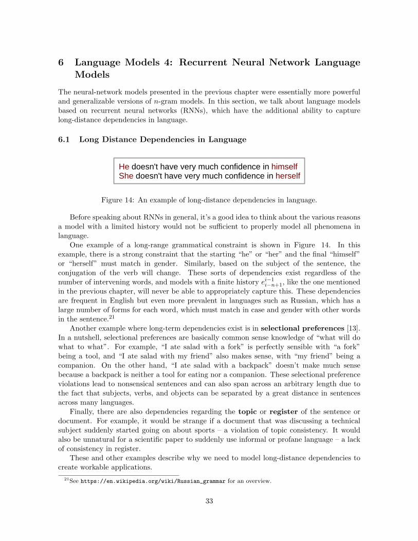
6 Language Models 4: Recurrent Neural Network LanguageModels

The neural-network models presented in the previous chapter were essentially more powerfuland generalizable versions of n-gram models. In this section, we talk about language modelsbased on recurrent neural networks (RNNs), which have the additional ability to capturelong-distance dependencies in language.

6.1 Long Distance Dependencies in Language

He doesn't have very much confidence in himselfShe doesn't have very much confidence in herself

Figure 14: An example of long-distance dependencies in language.

Before speaking about RNNs in general, it’s a good idea to think about the various reasonsa model with a limited history would not be su�cient to properly model all phenomena inlanguage.

One example of a long-range grammatical constraint is shown in Figure 14. In thisexample, there is a strong constraint that the starting “he” or “her” and the final “himself”or “herself” must match in gender. Similarly, based on the subject of the sentence, theconjugation of the verb will change. These sorts of dependencies exist regardless of thenumber of intervening words, and models with a finite history ei�1

i�n+1

, like the one mentionedin the previous chapter, will never be able to appropriately capture this. These dependenciesare frequent in English but even more prevalent in languages such as Russian, which has alarge number of forms for each word, which must match in case and gender with other wordsin the sentence.21

Another example where long-term dependencies exist is in selectional preferences [13].In a nutshell, selectional preferences are basically common sense knowledge of “what will dowhat to what”. For example, “I ate salad with a fork” is perfectly sensible with “a fork”being a tool, and “I ate salad with my friend” also makes sense, with “my friend” being acompanion. On the other hand, “I ate salad with a backpack” doesn’t make much sensebecause a backpack is neither a tool for eating nor a companion. These selectional preferenceviolations lead to nonsensical sentences and can also span across an arbitrary length due tothe fact that subjects, verbs, and objects can be separated by a great distance in sentencesacross many languages.

Finally, there are also dependencies regarding the topic or register of the sentence ordocument. For example, it would be strange if a document that was discussing a technicalsubject suddenly started going on about sports – a violation of topic consistency. It wouldalso be unnatural for a scientific paper to suddenly use informal or profane language – a lackof consistency in register.

These and other examples describe why we need to model long-distance dependencies tocreate workable applications.

21See https://en.wikipedia.org/wiki/Russian_grammar for an overview.

33

xt

×

(a) A single RNN time step

bh

Wxh

×

Whh

ht-1 + h

ttanh

x1

×

×h0 + tanh

(b) An unrolled RNN

Wxh

bh

Whh

×

× + tanh

x2

x3

×

× + tanh

x1

RNNh0

(c) A simplified view

x2

RNN

x3

RNN

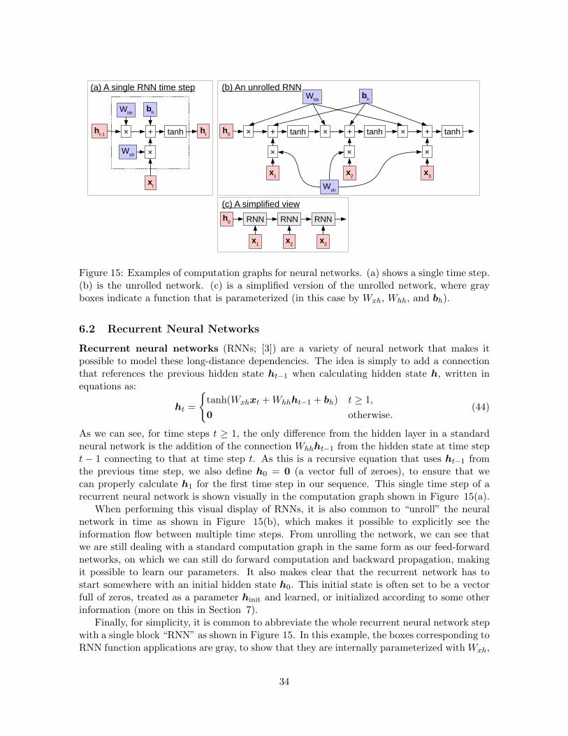
Figure 15: Examples of computation graphs for neural networks. (a) shows a single time step.(b) is the unrolled network. (c) is a simplified version of the unrolled network, where grayboxes indicate a function that is parameterized (in this case by W

xh

, Whh

, and b

h

).

6.2 Recurrent Neural Networks

Recurrent neural networks (RNNs; [3]) are a variety of neural network that makes itpossible to model these long-distance dependencies. The idea is simply to add a connectionthat references the previous hidden state h

t�1

when calculating hidden state h, written inequations as:

h

t

=

(tanh(W

xh

x

t

+Whh

h

t�1

+ b

h

) t � 1,

0 otherwise.(44)

As we can see, for time steps t � 1, the only di↵erence from the hidden layer in a standardneural network is the addition of the connection W

hh

h

t�1

from the hidden state at time stept � 1 connecting to that at time step t. As this is a recursive equation that uses h

t�1

fromthe previous time step, we also define h

0

= 0 (a vector full of zeroes), to ensure that wecan properly calculate h

1

for the first time step in our sequence. This single time step of arecurrent neural network is shown visually in the computation graph shown in Figure 15(a).

When performing this visual display of RNNs, it is also common to “unroll” the neuralnetwork in time as shown in Figure 15(b), which makes it possible to explicitly see theinformation flow between multiple time steps. From unrolling the network, we can see thatwe are still dealing with a standard computation graph in the same form as our feed-forwardnetworks, on which we can still do forward computation and backward propagation, makingit possible to learn our parameters. It also makes clear that the recurrent network has tostart somewhere with an initial hidden state h

0

. This initial state is often set to be a vectorfull of zeros, treated as a parameter h

init

and learned, or initialized according to some otherinformation (more on this in Section 7).

Finally, for simplicity, it is common to abbreviate the whole recurrent neural network stepwith a single block “RNN” as shown in Figure 15. In this example, the boxes corresponding toRNN function applications are gray, to show that they are internally parameterized with W

xh

,

34

x1

RNNh0

x2

RNN

x3

RNN

y*

�square_err

dl

dh3

=large

h1

h2

h3

dl

dh2

=med.dl

dh1

=smalldl

dh0

= tiny

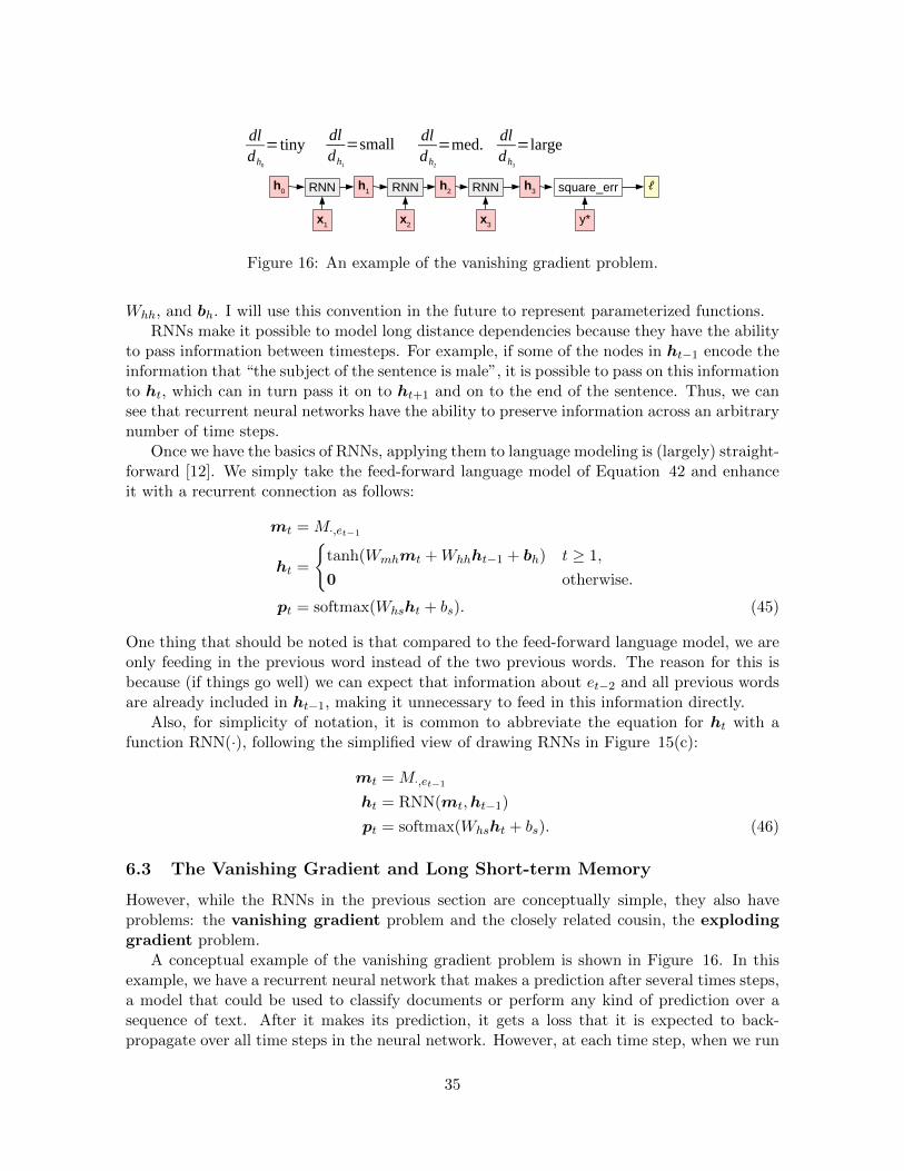
Figure 16: An example of the vanishing gradient problem.

Whh

, and b

h

. I will use this convention in the future to represent parameterized functions.RNNs make it possible to model long distance dependencies because they have the ability

to pass information between timesteps. For example, if some of the nodes in h

t�1

encode theinformation that “the subject of the sentence is male”, it is possible to pass on this informationto h

t

, which can in turn pass it on to h

t+1

and on to the end of the sentence. Thus, we cansee that recurrent neural networks have the ability to preserve information across an arbitrarynumber of time steps.

Once we have the basics of RNNs, applying them to language modeling is (largely) straight-forward [12]. We simply take the feed-forward language model of Equation 42 and enhanceit with a recurrent connection as follows:

m

t

= M·,et�1

h

t

=

(tanh(W

mh

m

t

+Whh

h

t�1

+ b

h

) t � 1,

0 otherwise.

p

t

= softmax(Whs

h

t

+ bs

). (45)

One thing that should be noted is that compared to the feed-forward language model, we areonly feeding in the previous word instead of the two previous words. The reason for this isbecause (if things go well) we can expect that information about e

t�2

and all previous wordsare already included in h

t�1

, making it unnecessary to feed in this information directly.Also, for simplicity of notation, it is common to abbreviate the equation for h

t

with afunction RNN(·), following the simplified view of drawing RNNs in Figure 15(c):

m

t

= M·,et�1

h

t

= RNN(mt

,ht�1

)

p

t

= softmax(Whs

h

t

+ bs

). (46)

6.3 The Vanishing Gradient and Long Short-term Memory

However, while the RNNs in the previous section are conceptually simple, they also haveproblems: the vanishing gradient problem and the closely related cousin, the explodinggradient problem.

A conceptual example of the vanishing gradient problem is shown in Figure 16. In thisexample, we have a recurrent neural network that makes a prediction after several times steps,a model that could be used to classify documents or perform any kind of prediction over asequence of text. After it makes its prediction, it gets a loss that it is expected to back-propagate over all time steps in the neural network. However, at each time step, when we run

35

ct-1

ct

u: tanh(×+)

i: σ(×+)

ht-1

ht

xt

o: σ(×+)

+

⊙ ⊙

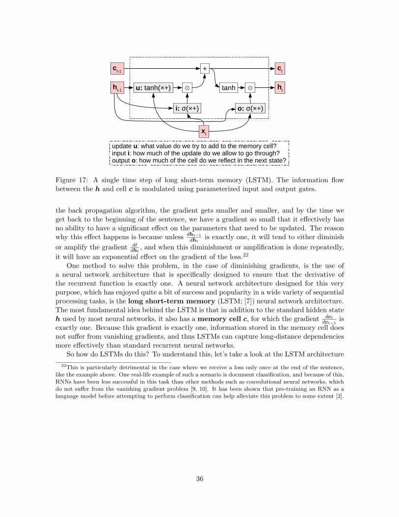
update u: what value do we try to add to the memory cell?input i: how much of the update do we allow to go through?output o: how much of the cell do we reflect in the next state?

tanh

Figure 17: A single time step of long short-term memory (LSTM). The information flowbetween the h and cell c is modulated using parameterized input and output gates.

the back propagation algorithm, the gradient gets smaller and smaller, and by the time weget back to the beginning of the sentence, we have a gradient so small that it e↵ectively hasno ability to have a significant e↵ect on the parameters that need to be updated. The reasonwhy this e↵ect happens is because unless dh

t�1

dht

is exactly one, it will tend to either diminish

or amplify the gradient d`

dht

, and when this diminishment or amplification is done repeatedly,

it will have an exponential e↵ect on the gradient of the loss.22

One method to solve this problem, in the case of diminishing gradients, is the use ofa neural network architecture that is specifically designed to ensure that the derivative ofthe recurrent function is exactly one. A neural network architecture designed for this verypurpose, which has enjoyed quite a bit of success and popularity in a wide variety of sequentialprocessing tasks, is the long short-term memory (LSTM; [7]) neural network architecture.The most fundamental idea behind the LSTM is that in addition to the standard hidden stateh used by most neural networks, it also has a memory cell c, for which the gradient dc

t

dct�1

isexactly one. Because this gradient is exactly one, information stored in the memory cell doesnot su↵er from vanishing gradients, and thus LSTMs can capture long-distance dependenciesmore e↵ectively than standard recurrent neural networks.

So how do LSTMs do this? To understand this, let’s take a look at the LSTM architecture

22This is particularly detrimental in the case where we receive a loss only once at the end of the sentence,like the example above. One real-life example of such a scenario is document classification, and because of this,RNNs have been less successful in this task than other methods such as convolutional neural networks, whichdo not su↵er from the vanishing gradient problem [9, 10]. It has been shown that pre-training an RNN as alanguage model before attempting to perform classification can help alleviate this problem to some extent [2].

36

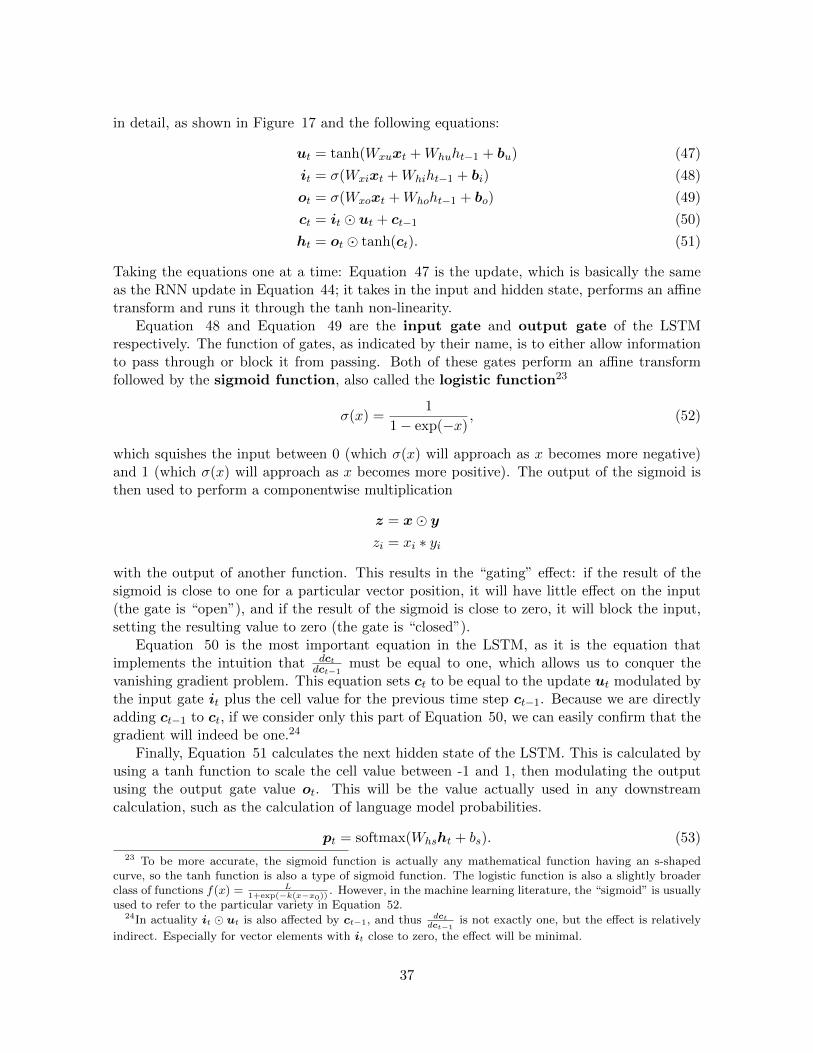
in detail, as shown in Figure 17 and the following equations:

u

t

= tanh(Wxu

x

t

+Whu

ht�1

+ b

u

) (47)

i

t

= �(Wxi

x

t

+Whi

ht�1

+ b

i

) (48)

o

t

= �(Wxo

x

t

+Who

ht�1

+ b

o

) (49)

c

t

= i

t

� u

t

+ c

t�1

(50)

h

t

= o

t

� tanh(ct

). (51)

Taking the equations one at a time: Equation 47 is the update, which is basically the sameas the RNN update in Equation 44; it takes in the input and hidden state, performs an a�netransform and runs it through the tanh non-linearity.

Equation 48 and Equation 49 are the input gate and output gate of the LSTMrespectively. The function of gates, as indicated by their name, is to either allow informationto pass through or block it from passing. Both of these gates perform an a�ne transformfollowed by the sigmoid function, also called the logistic function23

�(x) =1

1� exp(�x), (52)

which squishes the input between 0 (which �(x) will approach as x becomes more negative)and 1 (which �(x) will approach as x becomes more positive). The output of the sigmoid isthen used to perform a componentwise multiplication

z = x� y

zi

= xi

⇤ yi

with the output of another function. This results in the “gating” e↵ect: if the result of thesigmoid is close to one for a particular vector position, it will have little e↵ect on the input(the gate is “open”), and if the result of the sigmoid is close to zero, it will block the input,setting the resulting value to zero (the gate is “closed”).

Equation 50 is the most important equation in the LSTM, as it is the equation thatimplements the intuition that dc

t

dct�1

must be equal to one, which allows us to conquer thevanishing gradient problem. This equation sets c

t

to be equal to the update ut

modulated bythe input gate i

t

plus the cell value for the previous time step c

t�1

. Because we are directlyadding c

t�1

to c

t

, if we consider only this part of Equation 50, we can easily confirm that thegradient will indeed be one.24

Finally, Equation 51 calculates the next hidden state of the LSTM. This is calculated byusing a tanh function to scale the cell value between -1 and 1, then modulating the outputusing the output gate value o

t

. This will be the value actually used in any downstreamcalculation, such as the calculation of language model probabilities.

p

t

= softmax(Whs

h

t

+ bs

). (53)23 To be more accurate, the sigmoid function is actually any mathematical function having an s-shaped

curve, so the tanh function is also a type of sigmoid function. The logistic function is also a slightly broaderclass of functions f(x) = L

1+exp(�k(x�x0)). However, in the machine learning literature, the “sigmoid” is usually

used to refer to the particular variety in Equation 52.24In actuality i

t

� ut

is also a↵ected by ct�1

, and thus dctdct�1

is not exactly one, but the e↵ect is relatively

indirect. Especially for vector elements with it

close to zero, the e↵ect will be minimal.

37

6.4 Other RNN Variants

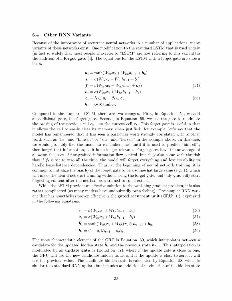
Because of the importance of recurrent neural networks in a number of applications, manyvariants of these networks exist. One modification to the standard LSTM that is used widely(in fact so widely that most people who refer to “LSTM” are now referring to this variant) isthe addition of a forget gate [4]. The equations for the LSTM with a forget gate are shownbelow:

u

t

= tanh(Wxu

x

t

+Whu

ht�1

+ b

u

)

i

t

= �(Wxi

x

t

+Whi

ht�1

+ b

i

)

f

t

= �(Wxf

x

t

+Whf

ht�1

+ b

f

) (54)

o

t

= �(Wxo

x

t

+Who

ht�1

+ b

o

)

c

t

= i

t

� u

t

+ f

t

� c

t�1

(55)

h

t

= o

t

� tanhct

.

Compared to the standard LSTM, there are two changes. First, in Equation 54, we addan additional gate, the forget gate. Second, in Equation 55, we use the gate to modulatethe passing of the previous cell c

t�1

to the current cell ct

. This forget gate is useful in thatit allows the cell to easily clear its memory when justified: for example, let’s say that themodel has remembered that it has seen a particular word strongly correlated with anotherword, such as “he” and “himself” or “she” and “herself” in the example above. In this case,we would probably like the model to remember “he” until it is used to predict “himself”,then forget that information, as it is no longer relevant. Forget gates have the advantage ofallowing this sort of fine-grained information flow control, but they also come with the riskthat if f

t

is set to zero all the time, the model will forget everything and lose its ability tohandle long-distance dependencies. Thus, at the beginning of neural network training, it iscommon to initialize the bias b

f

of the forget gate to be a somewhat large value (e.g. 1), whichwill make the neural net start training without using the forget gate, and only gradually startforgetting content after the net has been trained to some extent.

While the LSTM provides an e↵ective solution to the vanishing gradient problem, it is alsorather complicated (as many readers have undoubtedly been feeling). One simpler RNN vari-ant that has nonetheless proven e↵ective is the gated recurrent unit (GRU; [1]), expressedin the following equations:

r

t

= �(Wxr

x

t

+Whr

ht�1

+ b

r

) (56)

z

t

= �(Wxz

x

t

+Whz

ht�1

+ b

z

) (57)

h

t

= tanh(Wxh

x

t

+Whh

(rt

� h

t�1

) + b

h

) (58)

h

t

= (1� z

t

)ht�1

+ z

t

h

t

. (59)

The most characteristic element of the GRU is Equation 59, which interpolates between acandidate for the updated hidden state h

t

and the previous state h

t�1

. This interpolation ismodulated by an update gate z

t

(Equation 57), where if the update gate is close to one,the GRU will use the new candidate hidden value, and if the update is close to zero, it willuse the previous value. The candidate hidden state is calculated by Equation 58, which issimilar to a standard RNN update but includes an additional modulation of the hidden state

38

input by a reset gate r

t

calculated in Equation 56. Compared to the LSTM, the GRU hasslightly fewer parameters (it performs one less parameterized a�ne transform) and also doesnot have a separate concept of a “cell”. Thus, GRUs have been used by some to conservememory or computation time.

x1

RNNh1,0

x2

RNN

x3

RNN

RNNh2,0 RNN RNN

RNNh3,0 RNN RNN

x1

RNNh1,0

x2

RNN

x3

RNN

RNNh2,0 RNN RNN

RNNh3,0 RNN RNN

+ + +

+ + +

+ + +

(a) A stacked RNN (b) With residual connections

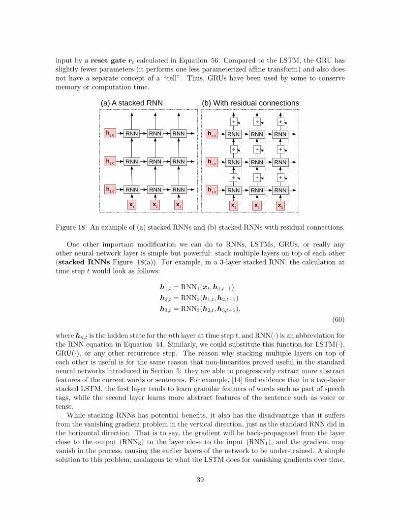
Figure 18: An example of (a) stacked RNNs and (b) stacked RNNs with residual connections.

One other important modification we can do to RNNs, LSTMs, GRUs, or really anyother neural network layer is simple but powerful: stack multiple layers on top of each other(stacked RNNs Figure 18(a)). For example, in a 3-layer stacked RNN, the calculation attime step t would look as follows:

h

1,t

= RNN1

(xt

,h1,t�1

)

h

2,t

= RNN2

(h1,t

,h2,t�1

)

h

3,t

= RNN3

(h2,t

,h3,t�1

),

(60)

where hn,t

is the hidden state for the nth layer at time step t, and RNN(·) is an abbreviation forthe RNN equation in Equation 44. Similarly, we could substitute this function for LSTM(·),GRU(·), or any other recurrence step. The reason why stacking multiple layers on top ofeach other is useful is for the same reason that non-linearities proved useful in the standardneural networks introduced in Section 5: they are able to progressively extract more abstractfeatures of the current words or sentences. For example, [14] find evidence that in a two-layerstacked LSTM, the first layer tends to learn granular features of words such as part of speechtags, while the second layer learns more abstract features of the sentence such as voice ortense.

While stacking RNNs has potential benefits, it also has the disadvantage that it su↵ersfrom the vanishing gradient problem in the vertical direction, just as the standard RNN did inthe horizontal direction. That is to say, the gradient will be back-propagated from the layerclose to the output (RNN

3

) to the layer close to the input (RNN1

), and the gradient mayvanish in the process, causing the earlier layers of the network to be under-trained. A simplesolution to this problem, analagous to what the LSTM does for vanishing gradients over time,

39

is residual networks (Figure 18(b)) [6]. The idea behind these networks is simply to addthe output of the previous layer directly to the result of the next layer as follows:

h

1,t

= RNN1

(xt

,h1,t�1

) + x

t

h

2,t

= RNN2

(h1,t

,h2,t�1

) + h

1,t

h

3,t

= RNN3

(h2,t

,h3,t�1

) + h

2,t

.

(61)

As a result, like the LSTM, there is no vanishing of gradients due to passing through theRNN(·) function, and even very deep networks can be learned e↵ectively.

6.5 Online, Batch, and Minibatch Training

As the observant reader may have noticed, the previous sections have gradually introducedmore and more complicated models; we started with a simple linear model, added a hiddenlayer, added recurrence, added LSTM, and added more layers of LSTMs. While these moreexpressive models have the ability to model with higher accuracy, they also come with a cost:largely expanded parameter space (causing more potential for overfitting) and more compli-cated operations (causing much greater potential computational cost). This section describesan e↵ective technique to improve the stability and computational e�ciency of training thesemore complicated networks, minibatching.

Up until this point, we have used the stochastic gradient descent learning algorithm in-troduced in Section 4.2 that performs updates according to the following iterative process.This type of learning, which performs updates a single example at a time is called onlinelearning.

Algorithm 1 A fully online training algorithm1: procedure Online2: for several epochs of training do3: for each training example in the data do4: Calculate gradients of the loss5: Update the parameters according to this gradient6: end for7: end for8: end procedure

In contrast, we can also think of a batch learning algorithm, which treats the entire dataset as a single unit, calculates the gradients for this unit, then only performs update aftermaking a full pass through the data.

These two update strategies have tradeo↵s.

• Online training algorithms usually find a relatively good solution more quickly, as theydon’t need to make a full pass through the data before performing an update.

• However, at the end of training batch, learning algorithms can be more stable, as theyare not overly influenced by the most recently seen training examples.

40

Algorithm 2 A batch learning algorithm1: procedure Batch2: for several epochs of training do3: for each training example in the data do4: Calculate and accumulate gradients of the loss5: end for6: Update the parameters according to the accumulated gradient7: end for8: end procedure

x1

Operations w/o Minibatching

W b

+tanh( )

W bx2

+tanh( )

W bx3

+tanh( )

Operations with Minibatching

x1 b

+tanh( )

x2x

3 concat

X BW

broadcast

Figure 19: An example of combining multiple operations together when minibatching.

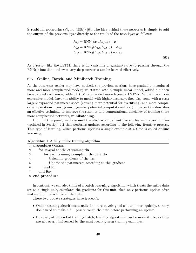
• Batch training algorithms are also more prone to falling into local optima; the random-ness in online training algorithms often allows them to bounce out of local minima andfind a better global solution.

Minibatching is a happy medium between these two strategies. Basically, minibatchedtraining is similar to online training, but instead of processing a single training example at atime, we calculate the gradient for n training examples at a time. In the extreme case of n = 1,this is equivalent to standard online training, and in the other extreme where n equals thesize of the corpus, this is equivalent to fully batched training. In the case of training languagemodels, it is common to choose minibatches of n = 1 to n = 128 sentences to process at asingle time. As we increase the number of training examples, each parameter update becomesmore informative and stable, but the amount of time to perform one update increases, so itis common to choose an n that allows for a good balance between the two.

One other major advantage of minibatching is that by using a few tricks, it is actuallypossible to make the simultaneous processing of n training examples significantly faster thanprocessing n di↵erent examples separately. Specifically, by taking multiple training examplesand grouping similar operations together to be processed simultaneously, we can realize largegains in computational e�ciency due to the fact that modern hardware (particularly GPUs,but also CPUs) have very e�cient vector processing instructions that can be exploited withappropriately structured inputs. As shown in Figure 19, common examples of this in neuralnetworks include grouping together matrix-vector multiplies from multiple examples into asingle matrix-matrix multiply or performing an element-wise operation (such as tanh) over

41

<s> that is an example<s> this is another </s>

RNN RNN RNN RNN RNN

softmax softmax softmax softmax softmax

lookup lookup lookup lookup lookup

loss( that this)

loss( is is)

loss( an another

)

loss( example

</s>)

loss( </s> </s>)

⊙ ⊙ ⊙ ⊙ ⊙

+

Input:

Recurrence:

Estimate:

Loss:

Masking:

Sum Time Steps:

Final Loss

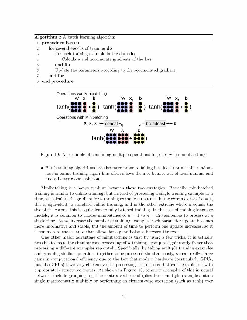
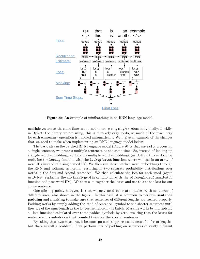
Figure 20: An example of minibatching in an RNN language model.

multiple vectors at the same time as opposed to processing single vectors individually. Luckily,in DyNet, the library we are using, this is relatively easy to do, as much of the machineryfor each elementary operation is handled automatically. We’ll give an example of the changesthat we need to make when implementing an RNN language model below.

The basic idea in the batched RNN language model (Figure 20) is that instead of processinga single sentence, we process multiple sentences at the same time. So, instead of looking upa single word embedding, we look up multiple word embeddings (in DyNet, this is done byreplacing the lookup function with the lookup batch function, where we pass in an array ofword IDs instead of a single word ID). We then run these batched word embeddings throughthe RNN and softmax as normal, resulting in two separate probability distributions overwords in the first and second sentences. We then calculate the loss for each word (againin DyNet, replacing the pickneglogsoftmax function with the pickneglogsoftmax batch

function and pass word IDs). We then sum together the losses and use this as the loss for ourentire sentence.

One sticking point, however, is that we may need to create batches with sentences ofdi↵erent sizes, also shown in the figure. In this case, it is common to perform sentencepadding and masking to make sure that sentences of di↵erent lengths are treated properly.Padding works by simply adding the “end-of-sentence” symbol to the shorter sentences untilthey are of the same length as the longest sentence in the batch. Masking works by multiplyingall loss functions calculated over these padded symbols by zero, ensuring that the losses forsentence end symbols don’t get counted twice for the shorter sentences.

By taking these two measures, it becomes possible to process sentences of di↵erent lengths,but there is still a problem: if we perform lots of padding on sentences of vastly di↵erent

42

lengths, we’ll end up wasting a lot of computation on these padded symbols. To fix thisproblem, it is also common to sort the sentences in the corpus by length before creatingmini-batches to ensure that sentences in the same mini-batch are approximately the samesize.

6.6 Further Reading

Because of the prevalence of RNNs in a number of tasks both on natural language and otherdata, there is significant interest in extensions to them. The following lists just a few otherresearch topics that people are handling:

What can recurrent neural networks learn?: RNNs are surprisingly powerful tools forlanguage, and thus many people have been interested in what exactly is going on insidethem. [8] demonstrate ways to visualize the internal states of LSTM networks, andfind that some nodes are in charge of keeping track of length of sentences, whether aparenthesis has been opened, and other salietn features of sentences. [11] show ways toanalyze and visualize which parts of the input are contributing to particular decisionsmade by an RNN-based model, by back-propagating information through the network.

Other RNN architectures: There are also quite a few other recurrent network architec-tures. [5] perform an interesting study where they ablate various parts of the LSTMand attempt to find the best architecture for particular tasks. [15] take it a step further,explicitly training the model to find the best neural network architecture.

6.7 Exercise

In the exercise for this chapter, we will construct a recurrent neural network language modelusing LSTMs.

Writing the program will entail:

• Writing a function such as lstm step or gru step that takes the input of the pre-vious time step and updates it according to the appropriate equations. For refer-ence, in DyNet, the componentwise multiply and sigmoid functions are dy.cmult anddy.logistic respectively.

• Adding this function to the previous neural network language model and measuring thee↵ect on the held-out set.

• Ideally, implement mini-batch training by using the lookup batch and pickneglogsoftmax batch

functionality implemented in DyNet.

Language modeling accuracy should be measured in the same way as previous exercises andcompared with the previous models.

Potential improvements to the model include: Implementing mini-batching and seeingspeed/stability improvements. Implementing dropout or regularization and measuring theaccuracy improvements.

43

References

[1] Junyoung Chung, Caglar Gulcehre, KyungHyun Cho, and Yoshua Bengio. Empirical evaluationof gated recurrent neural networks on sequence modeling. arXiv preprint arXiv:1412.3555, 2014.

[2] Andrew M Dai and Quoc V Le. Semi-supervised sequence learning. In Proceedings of the 29thAnnual Conference on Neural Information Processing Systems (NIPS), pages 3079–3087, 2015.

[3] Je↵rey L Elman. Finding structure in time. Cognitive science, 14(2):179–211, 1990.

[4] Felix A Gers, Jurgen Schmidhuber, and Fred Cummins. Learning to forget: Continual predictionwith lstm. Neural computation, 12(10):2451–2471, 2000.

[5] Klaus Gre↵, Rupesh Kumar Srivastava, Jan Koutnık, Bas R. Steunebrink, and Jurgen Schmid-huber. LSTM: A search space odyssey. CoRR, abs/1503.04069, 2015.

[6] Kaiming He, Xiangyu Zhang, Shaoqing Ren, and Jian Sun. Deep residual learning for imagerecognition. pages 770–778, 2016.

[7] Sepp Hochreiter and Jurgen Schmidhuber. Long short-term memory. Neural computation,9(8):1735–1780, 1997.

[8] Andrej Karpathy, Justin Johnson, and Li Fei-Fei. Visualizing and understanding recurrent net-works. arXiv preprint arXiv:1506.02078, 2015.

[9] Yoon Kim. Convolutional neural networks for sentence classification. In Proceedings of the 2014Conference on Empirical Methods in Natural Language Processing (EMNLP), pages 1746–1751,2014.

[10] Tao Lei, Regina Barzilay, and Tommi Jaakkola. Molding cnns for text: non-linear, non-consecutiveconvolutions. In Proceedings of the 2015 Conference on Empirical Methods in Natural LanguageProcessing (EMNLP), pages 1565–1575, 2015.

[11] Jiwei Li, Xinlei Chen, Eduard Hovy, and Dan Jurafsky. Visualizing and understanding neuralmodels in nlp. arXiv preprint arXiv:1506.01066, 2015.

[12] Tomas Mikolov, Martin Karafiat, Lukas Burget, Jan Cernocky, and Sanjeev Khudanpur. Recur-rent neural network based language model. In Proceedings of the 11th Annual Conference of theInternational Speech Communication Association (InterSpeech), pages 1045–1048, 2010.

[13] Philip Resnik. Selectional preference and sense disambiguation. In Proceedings of the ACLSIGLEX Workshop on Tagging Text with Lexical Semantics: Why, What, and How, pages 52–57.Washington, DC, 1997.

[14] Xing Shi, Inkit Padhi, and Kevin Knight. Does string-based neural mt learn source syntax?In Proceedings of the 2016 Conference on Empirical Methods in Natural Language Processing(EMNLP), pages 1526–1534, 2016.

[15] Barret Zoph and Quoc V Le. Neural architecture search with reinforcement learning. arXivpreprint arXiv:1611.01578, 2016.

44