53:102 GROUNDWATER Homework #7 -- Due: Monday, Oct. …
4
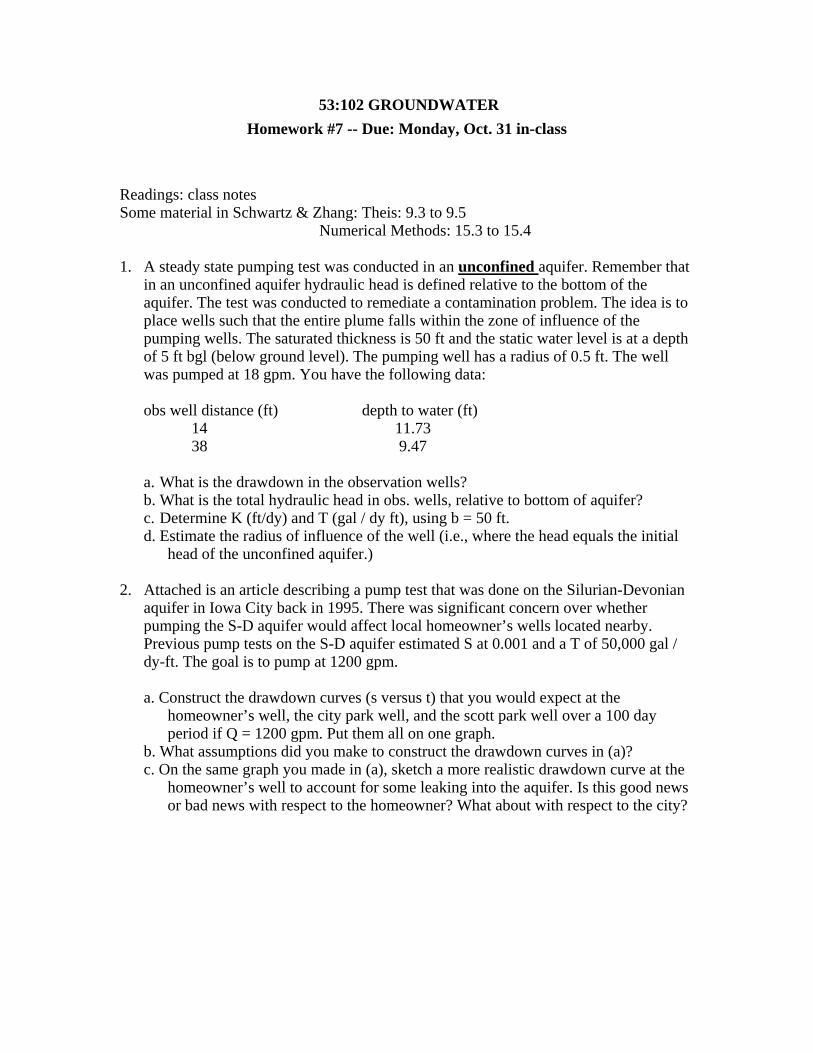
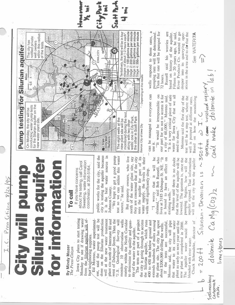
53:102 GROUNDWATER Homework #7 -- Due: Monday, Oct. 31 in-class Readings: class notes Some material in Schwartz & Zhang: Theis: 9.3 to 9.5 Numerical Methods: 15.3 to 15.4 1. A steady state pumping test was conducted in an unconfined aquifer. Remember that in an unconfined aquifer hydraulic head is defined relative to the bottom of the aquifer. The test was conducted to remediate a contamination problem. The idea is to place wells such that the entire plume falls within the zone of influence of the pumping wells. The saturated thickness is 50 ft and the static water level is at a depth of 5 ft bgl (below ground level). The pumping well has a radius of 0.5 ft. The well was pumped at 18 gpm. You have the following data: obs well distance (ft) depth to water (ft) 14 11.73 38 9.47 a. What is the drawdown in the observation wells? b. What is the total hydraulic head in obs. wells, relative to bottom of aquifer? c. Determine K (ft/dy) and T (gal / dy ft), using b = 50 ft. d. Estimate the radius of influence of the well (i.e., where the head equals the initial head of the unconfined aquifer.) 2. Attached is an article describing a pump test that was done on the Silurian-Devonian aquifer in Iowa City back in 1995. There was significant concern over whether pumping the S-D aquifer would affect local homeowner’s wells located nearby. Previous pump tests on the S-D aquifer estimated S at 0.001 and a T of 50,000 gal / dy-ft. The goal is to pump at 1200 gpm. a. Construct the drawdown curves (s versus t) that you would expect at the homeowner’s well, the city park well, and the scott park well over a 100 day period if Q = 1200 gpm. Put them all on one graph. b. What assumptions did you make to construct the drawdown curves in (a)? c. On the same graph you made in (a), sketch a more realistic drawdown curve at the homeowner’s well to account for some leaking into the aquifer. Is this good news or bad news with respect to the homeowner? What about with respect to the city?
Transcript of 53:102 GROUNDWATER Homework #7 -- Due: Monday, Oct. …
53:102 GROUNDWATER Homework #7 -- Due: Monday, Oct. 31 in-class
Readings: class notes Some material in Schwartz & Zhang: Theis: 9.3 to 9.5 Numerical Methods: 15.3 to 15.4 1. A steady state pumping test was conducted in an unconfined aquifer. Remember that
in an unconfined aquifer hydraulic head is defined relative to the bottom of the aquifer. The test was conducted to remediate a contamination problem. The idea is to place wells such that the entire plume falls within the zone of influence of the pumping wells. The saturated thickness is 50 ft and the static water level is at a depth of 5 ft bgl (below ground level). The pumping well has a radius of 0.5 ft. The well was pumped at 18 gpm. You have the following data:
obs well distance (ft) depth to water (ft)
14 11.73 38 9.47
a. What is the drawdown in the observation wells? b. What is the total hydraulic head in obs. wells, relative to bottom of aquifer? c. Determine K (ft/dy) and T (gal / dy ft), using b = 50 ft. d. Estimate the radius of influence of the well (i.e., where the head equals the initial
head of the unconfined aquifer.)
2. Attached is an article describing a pump test that was done on the Silurian-Devonian aquifer in Iowa City back in 1995. There was significant concern over whether pumping the S-D aquifer would affect local homeowner’s wells located nearby. Previous pump tests on the S-D aquifer estimated S at 0.001 and a T of 50,000 gal / dy-ft. The goal is to pump at 1200 gpm. a. Construct the drawdown curves (s versus t) that you would expect at the
homeowner’s well, the city park well, and the scott park well over a 100 day period if Q = 1200 gpm. Put them all on one graph.
b. What assumptions did you make to construct the drawdown curves in (a)? c. On the same graph you made in (a), sketch a more realistic drawdown curve at the
homeowner’s well to account for some leaking into the aquifer. Is this good news or bad news with respect to the homeowner? What about with respect to the city?
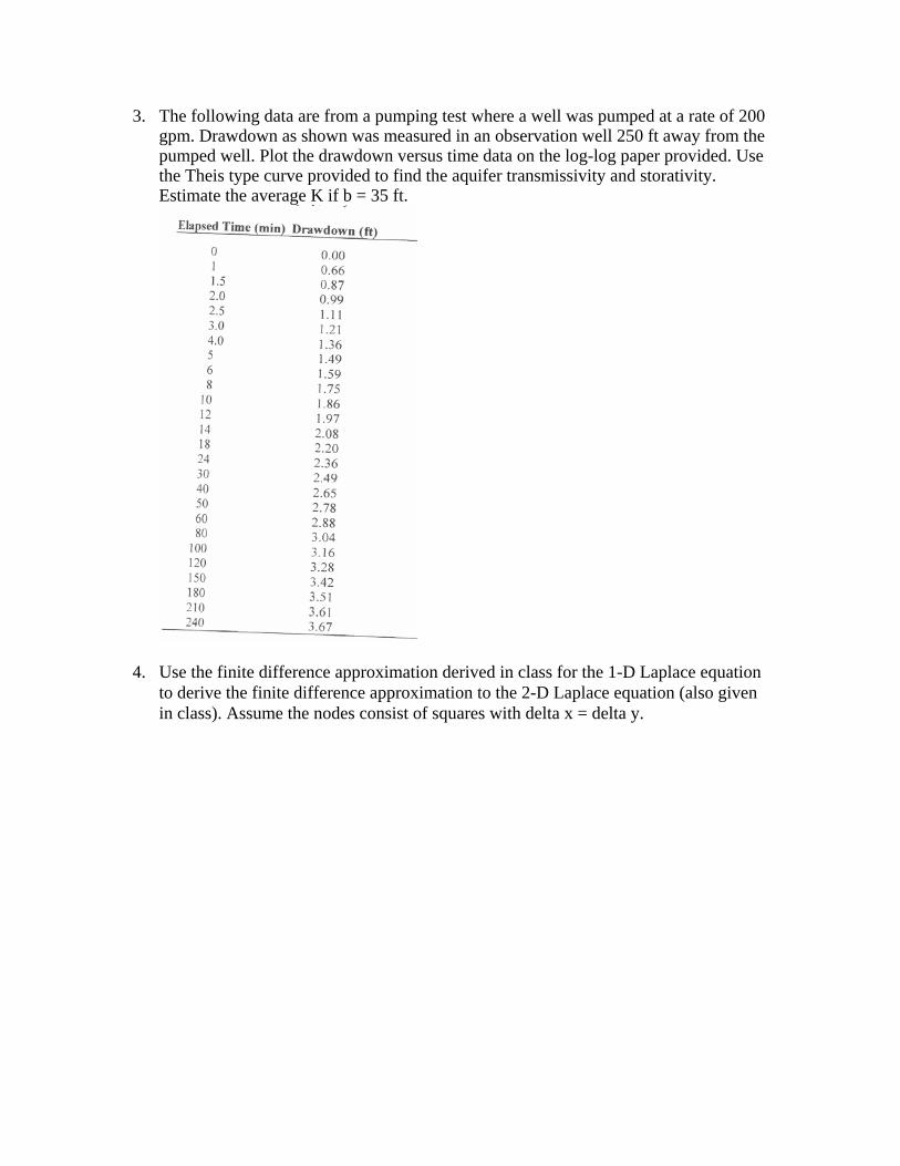
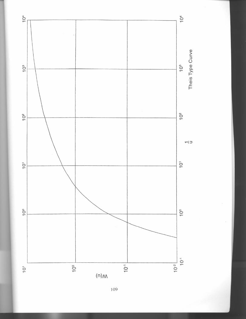
3. The following data are from a pumping test where a well was pumped at a rate of 200 gpm. Drawdown as shown was measured in an observation well 250 ft away from the pumped well. Plot the drawdown versus time data on the log-log paper provided. Use the Theis type curve provided to find the aquifer transmissivity and storativity. Estimate the average K if b = 35 ft.
4. Use the finite difference approximation derived in class for the 1-D Laplace equation
to derive the finite difference approximation to the 2-D Laplace equation (also given in class). Assume the nodes consist of squares with delta x = delta y.


![PIANO CONCERTO IN F 2nd Movement for Clarinets · 102 102 102 102 102 102 102 102 102 102 102 10 44 [Title]](https://static.fdocuments.net/doc/165x107/5e3946b540eed0696e2e90d2/piano-concerto-in-f-2nd-movement-for-clarinets-102-102-102-102-102-102-102-102-102.jpg)