5.1 Introduction - National Chiao Tung...
87
Signals_and_Systems_Simon Haykin & Barry Van Veen 1 Application to Communication Systems Application to Communication Systems CHAPTER 5. 5. 1 1 Introduction Introduction ♣ Modulation is basic to the operation of a communication system. 1. Modulation provides (1) shifting the range of frequencies into another ones suitable for transmission over the channel and (2) performing a corresponding shift back to the original frequency range after reception of the signal. 2. Modulation is defined as the process by which some characteristic of a carrier wave is varied in accordance with the message signal. Message signal → modulating wave modulating wave The result of modulation process → modulated wave modulated wave 5.2 5.2 Types of Modulation Types of Modulation 1. The form of carrier wave determine the specific type of modulation employed in a communication system. 2. Two most commonly used forms of carrier: sinusoidal wave and periodic pulse train. 3. Types of modulation: continuous continuous - - wave (CW) modulation and pulse modulation. wave (CW) modulation and pulse modulation.
Transcript of 5.1 Introduction - National Chiao Tung...
Signals_and_Systems_Simon Haykin amp Barry Van Veen
1
Application to Communication SystemsApplication to Communication SystemsCHAPTER
551 1 IntroductionIntroductionclubs Modulation is basic to the operation of a communication system1 Modulation provides (1) shifting the range of frequencies into another ones
suitable for transmission over the channel and (2) performing acorresponding shift back to the original frequency range after reception ofthe signal
2 Modulation is defined as the process by which some characteristic of a carrier wave is varied in accordance with the message signal
Message signal rarr modulating wavemodulating waveThe result of modulation process rarr modulated wavemodulated wave
52 52 Types of ModulationTypes of Modulation1 The form of carrier wave determine the specific type of modulation
employed in a communication system2 Two most commonly used forms of carrier sinusoidal wave and periodic
pulse train3 Types of modulation continuouscontinuous--wave (CW) modulation and pulse modulationwave (CW) modulation and pulse modulation
Signals_and_Systems_Simon Haykin amp Barry Van Veen
2
Application to Communication SystemsApplication to Communication SystemsCHAPTER
ContinuousContinuous--wave wave ((CWCW)) modulationmodulation1 Sinusoidal carrier wave ( ) cos( ( ))cc t A tφ= (51)
Ac equiv carrier amplitude φ(t) equiv angle
aa Amplitude modulationAmplitude modulation in which the carrier amplitude is varied with the in which the carrier amplitude is varied with the message signalmessage signal
bb Angle modulationAngle modulation in which the angle of the carrier is varied with the message in which the angle of the carrier is varied with the message signalsignal
ExamplesExamples
2 Subclasses of CW modulation
Fig 51Fig 513 Subclasses of amplitude modulation
1)1) Full amplitude modulation (double sidebandFull amplitude modulation (double sideband--transmitted carrier)transmitted carrier)2)2) Double sidebandDouble sideband--suppressed carrier modulationsuppressed carrier modulation3)3) Single sideband modulationSingle sideband modulation4)4) Vestigial sideband modulationVestigial sideband modulation
Linear modulation
Nonlinear modulation processNonlinear modulation process
4 Instantaneous radian frequency ωi(t)( )( )i
d ttdtφω = (52)
Signals_and_Systems_Simon Haykin amp Barry Van Veen
3
Application to Communication SystemsApplication to Communication SystemsCHAPTER
Figure 51 (p 426)Figure 51 (p 426)Amplitude- and angle-modulated signals for sinusoidal modulation (a) Carrier wave (b) Sinusoidal modulating signal (c) Amplitude-modulated signal (d) Angle-modulated signal
Signals_and_Systems_Simon Haykin amp Barry Van Veen
4
Application to Communication SystemsApplication to Communication SystemsCHAPTER
0( ) ( )
t
it dφ ω τ τ= int (53)
where it is assumed that the initial value is zero ie0
(0) ( ) 0i dφ ω τ τminusinfin
= =int5 The ordinary form of a sinusoidal wave
( ) cos( )c cc t A tω θ= + AAcc equivequiv amplitude amplitude ωωcc equivequiv radian frequency radian frequency θθ equivequiv phasephase
( ) ct tφ ω θ= +
( ) for alli ct tω ω=
6 When the instantaneous radian frequency ωi(t) is varied in accordance witha message signal m(t) we may write
( ) ( )i c ft k m tω ω= + (54)
0( ) ( )
t
c ft t k m dφ ω τ τ= + int
kkff is the frequency sensitivity is the frequency sensitivity factor of the modulatorfactor of the modulator
Frequency modulation (FM)
Signals_and_Systems_Simon Haykin amp Barry Van Veen
5
Application to Communication SystemsApplication to Communication SystemsCHAPTER
( )0( ) cos ( )
t
FM c c fs t A t k m dω τ τ= + int (55) Carrier amplitude Carrier amplitude
= constant= constant
7 When the angle φ(t) is varied in accordance with the message signal m(t) we may write
( ) ( )c pt t k m tφ ω= +kkpp is the phase sensitivity is the phase sensitivity
factor of the modulatorfactor of the modulatorPhase modulation
( ) cos( ( ))PM c c ps t A t k m tω= + (56) Carrier amplitude Carrier amplitude
= constant= constant
Pulse modulationPulse modulation1 Carrier wave
( ) ( )n
c t p t nTinfin
=minusinfin
= minussum
A periodic train of narrow pulsesA periodic train of narrow pulses
T equiv period p(t) equiv a pulse of relatively short duration and centered on the origin
2 When some characteristic parameter of p(t) is varied in accordance with themessage signal we have pulse modulation
Fig 52Fig 52
Signals_and_Systems_Simon Haykin amp Barry Van Veen
6
Application to Communication SystemsApplication to Communication SystemsCHAPTER
Figure 52 (p 428)Figure 52 (p 428)Pulse-amplitude modulation (a) Train of rectangular pulses as the carrier wave (b) Sinusoidal modulating signal (c) Pulse-amplitude modulated signal
Signals_and_Systems_Simon Haykin amp Barry Van Veen
7
Application to Communication SystemsApplication to Communication SystemsCHAPTER
3 Subclasses of pulse modulation1)1) Analog pulse modulation in which a characteristic parameter sucAnalog pulse modulation in which a characteristic parameter such as the h as the
amplitude duration or position of a pulse is varied continuousamplitude duration or position of a pulse is varied continuously with the ly with the message signalmessage signal
2)2) Digital pulse modulation in which the modulated signal is repreDigital pulse modulation in which the modulated signal is represented in sented in coded formcoded form
Two operations quantization and coding
Ex PCM = Pulse-code modulation
53 53 Benefits of ModulationBenefits of Modulationclubs Four practical benefits resulting from the use of modulation1 Modulation is used to shift the spectral content of a message signal to that it
lies inside the operating frequency band of a communication channelEx Speech signal with 300 to 3100 Hz frequency components
modulationmodulation 800 ~ 900 800 ~ 900 MHz in MHz in cellular radio systemcellular radio system
1) Subband 824-849 MHz used to receive signal
2) Subband 869-894 MHz used fortransmitting signals to mobile units
Signals_and_Systems_Simon Haykin amp Barry Van Veen
8
Application to Communication SystemsApplication to Communication SystemsCHAPTER
2 Modulation provides a mechanism for putting the information content of a message signal into a form that may be less vulnerable to noise orinterference
3 Modulation permits the use of multiplexing4 Modulation makes it possible for the physical size of the transmitting or
receiving antenna to assume a practical valueclubs Detailed description See pp429 ~ 430 textbook
54 54 Full Amplitude ModulationFull Amplitude Modulation1 Sinusoidal carrier wave
( ) cos( )c cc t A tω= (57)
2 Amplitude modulation (AM) is defined as a process in which the amplitude of the carrier is varied in proportion to a message signal m(t) according to theformula
[ ]( ) 1 ( ) cos( )c a cs t A k m t tω= + (58) kkaa is the amplitude sensitivity is the amplitude sensitivity
factor of the modulatorfactor of the modulators(t) = modulated signal m(t) = message signa
541 541 Performance of ModulationPerformance of Modulation
Angle φ(t) is assumed to be zero
Signals_and_Systems_Simon Haykin amp Barry Van Veen
9
Application to Communication SystemsApplication to Communication SystemsCHAPTER
1 The envelope of the AM wave s(t)( ) 1 ( )c aa t A k m t= + (59)
2 Two cases arise depending on the magnitude of kam(t) compare with unity1) Undermodulation which is governed by the condition
[ ]( ) 1 ( ) for all tc aa t A k m t= +
( ) 1 for allak m t tle 1 + kam(t) gt 0The envelope of the AM wave is then simplified as
(510)
2) Overmodulation which is governed by the weaker condition( ) 1 for someak m t tgt
3 Percentage modulation equiv kam(t)times 100542 542 Generation of AM WaveGeneration of AM Wave1 Another form of the modulated AM wave s(t)
[ ]( ) ( ) cos( )a c cs t k m t B A tω= + (511) BB = 1= 1kkaa equivequiv a a biasbias that is added to the message signal that is added to the message signal mm((tt) before modulation) before modulation
Signals_and_Systems_Simon Haykin amp Barry Van Veen
10
Application to Communication SystemsApplication to Communication SystemsCHAPTER
2 Block diagram for generating an AM wave Fig 53Fig 53Basically it consists of two functional blocks1)1) An adder which adds the bias An adder which adds the bias BB to the incoming message signal to the incoming message signal mm((tt))2)2) A multiplier which multiplies the adder output A multiplier which multiplies the adder output ((mm((tt) + ) + BB)) by the carrier wave by the carrier wave
AAcccoscos((ωωcctt)) producing the AM wave producing the AM wave ss((tt))
Figure 53 (p 432)Figure 53 (p 432)Spectrum involving an adder and multiplier for generating an AM wave
v equiv ω p equiv π
543 543 Possible Waveforms of AM WavePossible Waveforms of AM Wave1 Fig 54Fig 54 illustrates the waveforms generated by the amplitude modulation
processPart (a) message signal Part (a) message signal mm((tt) (b) percentage modulation = 667 and (c) 1667) (b) percentage modulation = 667 and (c) 1667
Signals_and_Systems_Simon Haykin amp Barry Van Veen
11
Application to Communication SystemsApplication to Communication SystemsCHAPTER
Figure 54 (p 432)Figure 54 (p 432)Amplitude modulation for a varying percentage of modulation (a) Message signal m(t) (b) AM wave for |kam(t)| lt 1 for all t where ka is the amplitude sensitivity of the modulator This case represents undermodulation (c) AM wave for |kam(t)| gt 1 some of the time This case represents overmodulation
Signals_and_Systems_Simon Haykin amp Barry Van Veen
12
Application to Communication SystemsApplication to Communication SystemsCHAPTER
2 Important conclusionThe envelope of the AM wave has a waveform that bears a oneThe envelope of the AM wave has a waveform that bears a one--toto--one one correspondence with that of the message signal if the percentagecorrespondence with that of the message signal if the percentage modulation is modulation is less than or equal to 100less than or equal to 100
clubs If percentage modulation gt 100 the modulated wave is said to suffer fromenvelope distortion
544 544 Does FullDoes Full--Amplitude Modulation Satisfy the Linearity Property Amplitude Modulation Satisfy the Linearity Property 1 Amplitude modulation as defined in Eq (58) fails the linearity test in a
strict sense2 Demonstration
1) 1) Suppose that Suppose that mm((tt) = ) = mm11(t) + (t) + mm22((tt) Let ) Let ss11((tt) and ) and ss22((tt) denote the AM waves ) denote the AM waves produced by these two components acting separatelyproduced by these two components acting separately
2) 2) Let the operator Let the operator HH denote the amplitude modulation process therefore we denote the amplitude modulation process therefore we havehave
[ ]1 1( ) 1 ( ) cos( )c a cs t A k m t tω= + [ ]2 2( ) 1 ( ) cos( )c a cs t A k m t tω= +and
( )1 2 1 2
1 2
( ) ( ) 1 ( ) ( ) cos( )
( ) ( )c a cH m t m t A k m t m t t
s t s t
ω+ = + +⎡ ⎤⎣ ⎦ne +
Signals_and_Systems_Simon Haykin amp Barry Van Veen
13
Application to Communication SystemsApplication to Communication SystemsCHAPTER
The superposition principle is violatedThe superposition principle is violated
545 545 FrequencyFrequency--Domain Description of Amplitude ModulationDomain Description of Amplitude Modulation1 Fourier transform pairs
( ) ( )FTs t S jωlarr⎯⎯rarr and ( ) ( )FTm t M jωlarr⎯⎯rarr
Message Message spectrumspectrum
2 Fourier transform of Accos(ωct)
[ ]( ) ( )c c cAπ δ ω ω δ ω ωminus + +
cFourier transform of m(t)cos( t)ω
[ ]1 ( ) ( )2 c cM j j M j jω ω ω ωminus + +
3 Fourier transform of the AM wave of Eq (58)
[ ]
[ ]
( ) ( ) ( )1 + ( ( )) ( ( )) 2
c c c
a c c c
S j A
k A M j M j
ω π δ ω ω δ ω ω
ω ω ω ω
= minus + +
minus + +(512)
Fig 55Fig 55
Signals_and_Systems_Simon Haykin amp Barry Van Veen
14
Application to Communication SystemsApplication to Communication SystemsCHAPTER
Figure 55 (p 434)Figure 55 (p 434)Spectral content of AM wave (a) Magnitude spectrum of message signal (b) Magnitude spectrum of the AM wave showing the compositions of the carrier and the upper and lower sidebands
v equiv ω p equiv π
clubs Descriptions for Fig 55Fig 55
1)1) The message signal is band limited to the interval The message signal is band limited to the interval minusminus ωωmm lele ωω lele ωωmm2)2) ωωmm equivequiv the message bandwidth of the message bandwidth of mm((tt) in rads) in rads3)3) The spectrum of The spectrum of SS((jjωω) consists of two impulse functions weighted by the factor ) consists of two impulse functions weighted by the factor
ππAAcc and occurring at and occurring at plusmnplusmn ωωcc and two versions of the message spectrum shifted in and two versions of the message spectrum shifted in frequency by frequency by plusmnplusmn ωωcc and scaled in amplitude by (12)and scaled in amplitude by (12)kkaaAAcc
The spectrum of the AM wave as The spectrum of the AM wave as depicted in Fig 55 (b) is depicted in Fig 55 (b) is fullfull
Signals_and_Systems_Simon Haykin amp Barry Van Veen
15
Application to Communication SystemsApplication to Communication SystemsCHAPTER
4) 4) Upper sideband Upper sideband equivequiv the spectrum lying above the spectrum lying above ωωcc or below or below minusminus ωωcc5) Lower sideband 5) Lower sideband equivequiv the spectrum lying below the spectrum lying below ωωcc or above or above minusminus ωωcc
The condition ωc gt ωm is a necessary condition for the sidebands not to overlap
6) 6) Highest frequency component of the AM wave Highest frequency component of the AM wave equivequiv ωωcc + + ωωmm7) Lowest frequency component of the AM wave 7) Lowest frequency component of the AM wave equivequiv ωωcc minusminus ωωmm8) The difference between these two frequencies defines the tran8) The difference between these two frequencies defines the transmission smission
bandwidth bandwidth ωωTT for an AM wave for an AM wave
2T mω ω= (513)
Example 51 Full Amplitude Modulation for Sinusoidal Modulating SignalConsider a modulating wave m(t) that consists of a single tone or frequency component that is
0 0( ) cos( )m t A tω=
where A0 is the amplitude of the modulating wave and ω0 is its radian frequency (See Fig 56(a)Fig 56(a)) The sinusoidal carrier wave c(t) has amplitude Ac and radian frequency ωc (See Fig 56(b)Fig 56(b)) Evaluate the time-domain and frequency-domain characteristics of the AM wave
Signals_and_Systems_Simon Haykin amp Barry Van Veen
16
Application to Communication SystemsApplication to Communication SystemsCHAPTER
Figure 56 (p Figure 56 (p 435)435)Time-domain (on the left) and frequency-domain (on the right) characteristics of AM produced by a sinusoidal modulating wave (a) Modulating wave (b) Carrier wave (c) AM wave
v equiv ω p equiv π
Signals_and_Systems_Simon Haykin amp Barry Van Veen
17
Application to Communication SystemsApplication to Communication SystemsCHAPTER
ltltSolgtSolgt1 The AM wave is described by
[ ]0( ) 1 cos( ) cos( )c cs t A t tμ ω ω= + (514) where 0ak Aμ =
clubsclubs The dimensionless constant The dimensionless constant μμ for a sinusoidal modulating wave is called the for a sinusoidal modulating wave is called the modulation factormodulation factor and equals the percentage modulation when it is expressedand equals the percentage modulation when it is expressednumerically as a percentage numerically as a percentage
clubsclubs To avoid envelope distortion due to To avoid envelope distortion due to overmodulationovermodulation the modulation factor the modulation factor μμ mustmustbe kept below unitybe kept below unity
clubsclubs Figure 56(c)Figure 56(c) is a sketch of is a sketch of ss((tt) for ) for μμ less than unityless than unity2 Let Amax and Amin denote the maximum and minimum values respectively of
the envelope of the modulated wave Then form Eq(514) we get
max
min
(1 )(1 )
c
c
A AA A
μμ
+=
minusmax min
max min
A AA A
μ minus=
+
3 Expressing the product of the two cosines in Eq (514) as the sum of two sinusoidal waves one having frequency ωc + ω0 and the other havingfrequency ωc-ω0 we get
Signals_and_Systems_Simon Haykin amp Barry Van Veen
18
Application to Communication SystemsApplication to Communication SystemsCHAPTER
102
102
( ) cos( ) cos[( ) ]
cos[( ) ]
c c c c
c c
s t A t A t
A t
ω μ ω ω
μ ω ω
= + +
+ minus
4 Fourier transform of s(t)
10 02
10 02
( ) [ ( ) ( )]
[ ( ) ( )]
[ ( ) ( )]
c c c
c c c
c c c
S j A
A
A
ω π δ ω ω δ ω ω
πμ δ ω ω ω δ ω ω ω
πμ δ ω ω ω δ ω ω ω
= minus + +
+ minus minus + + +
+ minus + + + minus
Thus in ideal terms the spectrum of a full AM wave for the spThus in ideal terms the spectrum of a full AM wave for the special case of ecial case of sinusoidal modulation consists of impulse functions at sinusoidal modulation consists of impulse functions at plusmnplusmn ωωcc ωωcc plusmnplusmn ωω00 and and--ωωc c plusmnplusmn ωω 00 as depicted inas depicted in Fig 56(c)Fig 56(c)
Example 52 Average Power of Sinusoidally Modulated SignalContinuing with Example 51 investigate the effect of varying the modulation factor μ on the power content of the AM wave ltltSolgtSolgt1 In practice the AM wave s(t) is a voltage or current signal
Signals_and_Systems_Simon Haykin amp Barry Van Veen
19
Application to Communication SystemsApplication to Communication SystemsCHAPTER
2 In either case the average power delivered to a 1-ohm load resistor by s(t) is composed of three components whose values are derived from Eq (115) asfollows
1 22
1 2 281 2 28
Carrier power
Upper side- frequency power
Lower side- frequency power
c
c
c
A
A
A
μ
μ
=
=
=
3 The ratio of the total sideband power to the total power in the modulated wave is therefore equal th μ 2(2 + μ 2) which depends only on the modulationfactor μ If μ = 1 (ie if 100 modulation is used) the total power in the twoside frequencies of the resulting AM wave is only one-third of the total powerin the modulated wave
4 Figure 57Figure 57 shows the percentage of total power in both side frequencies and in the carrier plotted against the percentage modulation
Signals_and_Systems_Simon Haykin amp Barry Van Veen
20
Application to Communication SystemsApplication to Communication SystemsCHAPTER
Figure 57 (p 437)Figure 57 (p 437)Variations of carrier power and side-frequency power with percentage modulation of AM wave for the case of sinusoidal modulation
546 546 Spectral OverlapSpectral Overlap1 When ωc lt ωm the modulated signal
s(t) undergoes frequency distortiondue to spectral overlap
Fig 58Fig 58clubs Assume that S(jω) is real valued2 The spectral overlap is produced by two movements
1)1) Movement of the lower sideband into the negative frequency rangeMovement of the lower sideband into the negative frequency range2)2) Movement of the image of the lower sideband into the positive frMovement of the image of the lower sideband into the positive frequency rangeequency range
3 For avoiding the spectral overlap problem the necessary condition is
c mω ωge
Signals_and_Systems_Simon Haykin amp Barry Van Veen
21
Application to Communication SystemsApplication to Communication SystemsCHAPTER
Figure 58 (p 438)Figure 58 (p 438)Spectral overlap phenomenon in amplitude modulation The phenomenon arises when the carrier frequency ωc is less than the highest frequency component ωm of the modulating signal
v equiv ω p equiv π
547 547 Demodulation of AM WaveDemodulation of AM Wave1 The envelope detector provides a simple yet effective device for the
demodulation of a narrowband AM signal for which the percentage modulation is less than 100
clubsclubs Narrowband means that the carrier is large compared with the mesNarrowband means that the carrier is large compared with the message bandwidthsage bandwidth2 Circuit diagram of an envelope detector Fig 59Fig 59
1) 1) The diode is ideal presenting zero impedance to current flow inThe diode is ideal presenting zero impedance to current flow in the forwardthe forward--biased region and infinite impedance in the reversebiased region and infinite impedance in the reverse--biased region biased region
Signals_and_Systems_Simon Haykin amp Barry Van Veen
22
Application to Communication SystemsApplication to Communication SystemsCHAPTER
Figure 59 (p 438)Figure 59 (p 438)Envelope detector illustrated by (a) circuit diagram (b) AM wave input and (c) envelope detector output assuming ideal conditions
Signals_and_Systems_Simon Haykin amp Barry Van Veen
23
Application to Communication SystemsApplication to Communication SystemsCHAPTER
2) 2) The AM signal applied to the envelope is supplied by a voltage sThe AM signal applied to the envelope is supplied by a voltage source of ource of internal resistance internal resistance RRss
3) The load resistance 3) The load resistance RRll is large compared with the source resistance is large compared with the source resistance RRss During Duringthe charging process the time constant is effectively equathe charging process the time constant is effectively equal to l to RRssCC This time This time constant must be short compared with the carrier period 2constant must be short compared with the carrier period 2ππωωcc that is that is
2s
c
R πω
ltlt (515)
3 The discharging time constant is equal to RlCRRllCC must be large such that the capacitor discharges slowly but notmust be large such that the capacitor discharges slowly but not so so large that the capacitor voltage will not discharge at the maximlarge that the capacitor voltage will not discharge at the maximum rate um rate of change of the modulating wave ieof change of the modulating wave ie2 2
lc m
R Cπ πω ω
ltlt ltlt (516) ωm equiv message
bandwidth
clubs Output ripple can be removed by low-pass filter
Signals_and_Systems_Simon Haykin amp Barry Van Veen
24
Application to Communication SystemsApplication to Communication SystemsCHAPTER
55 55 Double SidebandDouble Sideband--Suppressed ModulationSuppressed Modulation1 In full AM carrier wave c(t) is completely independent of the message signal
m(t)
Transmission of carrier wave A waste of power
2 To overcome this shortcoming we may suppress the carrier component from the modulated wave resulting in double sideband-suppressed carrier(DSB-SC) modulation
3 DSB-SC modulated signal( ) ( ) ( ) cos( ) ( )c cs t c t m t A t m tω= = (517)
clubs This modulated signal undergoes a phase reversal whenever the messagesignal m(t) crosses zero as illustrated in Fig 510Fig 510(a)(a) Message signal Message signal (b)(b) DSBDSB--SC modulated wave resulting from multiplication of the message SC modulated wave resulting from multiplication of the message
signal by the sinusoidal carrier wave signal by the sinusoidal carrier wave
Signals_and_Systems_Simon Haykin amp Barry Van Veen
25
Application to Communication SystemsApplication to Communication SystemsCHAPTER
Figure 510 (p 440)Figure 510 (p 440)Double-sideband-suppressed carrier modulation (a) Message signal (b) DSB-SC modulated wave resulting from multiplication of the message signal by the sinusoidal carrier wave
551 551 FrequencyFrequency--Domain DescriptionDomain Description1 Fourier transform of modulated signal s(t)
1( ) [ ( ( )) ( ( ))]2 c c cS j A M j M jω ω ω ω ω= minus + + (518)
where M(jω) equiv Fourier transform of m(t) minus ωm le ω le ωmFig 511 (a) and (b)Fig 511 (a) and (b)
Signals_and_Systems_Simon Haykin amp Barry Van Veen
26
Application to Communication SystemsApplication to Communication SystemsCHAPTER
Figure 511 (p 441)Figure 511 (p 441)Spectral content of DSB-SC modulated wave (a) Magnitude spectrum of message signal (b) Magnitude spectrum of DSB-SC modulated wave consisting of upper and lower sidebands only
v equiv ω p equiv π
clubs The modulation process simply translates the spectrum of the message signal by plusmn ωc
clubs Transmission bandwidth = 2 ωm2 A device for achieving DSB-SC is called a product modulator or simply
multiplierFig 512 (a)Fig 512 (a) shows the block diagram of a product modulator
Signals_and_Systems_Simon Haykin amp Barry Van Veen
27
Application to Communication SystemsApplication to Communication SystemsCHAPTER
Figure 512 (p 441)Figure 512 (p 441)(a) Product modulator for generating the DSB-SC modulated wave (b) Coherent detector for demodulation of the DSB-SC modulated wave
v equiv ω p equiv π
552 552 Coherent DetectionCoherent Detection1 The message signal m(t) may be recovered from DSB-SC
Fig 512 (b)Fig 512 (b)ss((tt) ) timestimes locally generated sinusoidal wave = locally generated sinusoidal wave = vv((tt))vv((tt) filtered by a Low) filtered by a Low--pass filterpass filter
Local oscillator
2 The local oscillator should be exactly coherent or synchronized in both frequency and phase with the carrier wave c(t)
Signals_and_Systems_Simon Haykin amp Barry Van Veen
28
Application to Communication SystemsApplication to Communication SystemsCHAPTER
Coherent detection or synchronization demodulation3 Derivation for coherent detection
1) Local oscillator cos(ωct + φ )2) Product modulator output
( ) cos( ) ( )cos( ) cos( ) ( )
1 1cos( ) ( ) cos(2 ) ( )2 2
c
c c c
c c c
v t t s tA t t m t
A m t A t m t
ω φω ω φ
φ ω φ
= += +
= + +(519)
1 cos( ) ( )2 cA m tφ
1 cos(2 ) ( )2 c cA t m tω φ+
A scaled version of the original message signal m(t)
DSBDSB--SC modulated signal with carrier SC modulated signal with carrier frequency 2 frequency 2 ωωcc
3) Magnitude spectrum Fig 5134) To clear separate two component of v(t) the original carrier frequency ωc
must satisfy the condition
Signals_and_Systems_Simon Haykin amp Barry Van Veen
29
Application to Communication SystemsApplication to Communication SystemsCHAPTER
Figure 513 (p 442)Figure 513 (p 442)Magnitude spectrum of the product modulator output v(t) in the coherent detector of Fig 512(b)
v equiv ω p equiv π
2 c m mω ω ωminus gt c mω ωgt (520) ωωmm equivequiv message bandwidthmessage bandwidth
4 Specification of low-pass filter1) 1) The cutoff frequency must be The cutoff frequency must be ωωm m 2) The transition band must be 2) The transition band must be ωωm m ≦≦ ωω ≦≦ ωωc c ωωm m
Thus the overall output in Thus the overall output in Fig 512(b)Fig 512(b) is given byis given by1( ) cos( ) ( )2o cv t A m tφ= (521)
cosφ equiv attenuation factor
Signals_and_Systems_Simon Haykin amp Barry Van Veen
30
Application to Communication SystemsApplication to Communication SystemsCHAPTER
5 (1) Demodulated signal vo(t) is proportional to m(t) when the error phase φis a constant
(2) Demodulated signal is maximum when φ = 0 and has a minimum zero when φ = plusmn π2
Example 53 Sinusoidal DSB-SC ModulationConsider again the sinusoidal modulating signal
0 0( ) cos( )m t A tω=
( ) cos( )c cc t A tω=with amplitude A0 and frequency ω0 see Fig 514(a) The carrier wave is
with amplitude Ac and frequency ωc see Fig 514(b) Investigate the time-domain and frequency-domain characteristics of the corresponding DSB-SC modulated waveltltSolgtSolgt
clubs φ = plusmn π2 represents the quadrature null effect of the coherent detector
1 The modulated DSB-SC signal is defined by
0 0
0 0 0 0
( ) cos( ) cos( )1 1cos[( ) ] cos[( ) ]2 2
c c
c c c c
s t A A t t
A A t A A t
ω ω
ω ω ω ω
=
= + + minus
Signals_and_Systems_Simon Haykin amp Barry Van Veen
31
Application to Communication SystemsApplication to Communication SystemsCHAPTER
2 The Fourier transform of s(t) is given by
0 0 0
0 0
1( ) cos[ ( ) ( )]2
( ) ( )
c c c
c c
S j A Aω π δ ω ω ω δ ω ω ω
δ ω ω ω δ ω ω ω
= minus minus + + +
+ minus + + + minus
which consists of four weighted impulse functions at the frequencies ωc+ ω0-ωc- ω0 ωc- ω0 and- ωc+ ω0 as illustrated in the right-hand side of Fig Fig 514(c)514(c)
3 This Fourier transform differs from that depicted in the right-hand side of Fig Fig 56(c)56(c) for the corresponding example of full AM in one important respect The impulse functions at plusmn ωc due to the carrier are removed
4 Application of the sinusoidally modulated DSB-SC signal to the product modulator of Fig 512(b) yields the output (assuming φ = 0)
0 0 0
0 0 0 0 0
1( ) cos( ) cos[( ) ] cos[( ) ]21 cos[(2 ) ] cos( ) cos[(2 ) ] cos( )4
c c c c
c c c
v t A A t t t
A A t t t t
ω ω ω ω ω
ω ω ω ω ω ω
= + + minus
= + + + minus +
Signals_and_Systems_Simon Haykin amp Barry Van Veen
32
Application to Communication SystemsApplication to Communication SystemsCHAPTER
Figure 514 (p Figure 514 (p 443)443)Time-domain (on the left) and frequency-domain (on the right) characteristics of DSB-SC modulation produced by a sinusoidal modulating wave (a) Modulating wave (b) Carrier wave (c) DSB-SC modulated wave Note that ω= 2πƒ
v equiv ω p equiv π
Signals_and_Systems_Simon Haykin amp Barry Van Veen
33
Application to Communication SystemsApplication to Communication SystemsCHAPTER
5 The first two sinusoidal terms of v(t) are produced by the upper side frequency and the last two sinusoidal terms are produced by the lower side frequency
6 With ωcgt ω0 the first and third sinusoidal terms of frequencies 2ωc+ ω0 and 2ωc-ω0 respectively are removed by the low-pass filter of Fig 512(b)Fig 512(b) which leaves the second and fourth sinusoidal terms of frequency ω0 as the only output of the filter The coherent detector output thus reproduces the original modulating wave
7 Note however that this output appears as two equal terms one derived from the upper side frequency and the other from the lower side frequency We therefore conclude that for the transmission of the sinusoidal signal A0 cos(ω0t) only one side frequency is necessary (The issue will be discussed further in Section 57Section 57)
553 553 CostasCostas ReceiverReceiver1 Costas receiver Fig 515Fig 5152 This receiver consists of two coherent detector supplied with the same input
ie the incoming DSB-Sc wave
cos(2 ) ( )c cA f t m tπ but with individual local oscillator signals that are in phase duadrature with respect to each other
In-phase coherent detector (I-Channel) and quadrature-phase coherent detector (Q-Channel)
Signals_and_Systems_Simon Haykin amp Barry Van Veen
34
Application to Communication SystemsApplication to Communication SystemsCHAPTER
Figure 515 (p 445)Figure 515 (p 445)Costas receiver
v equiv ω p equiv π
Signals_and_Systems_Simon Haykin amp Barry Van Veen
35
Application to Communication SystemsApplication to Communication SystemsCHAPTER
56 56 QuadratureQuadrature--Carrier MultiplexingCarrier Multiplexing
Figure 516 (p 446)Figure 516 (p 446)Quadrature-carrier multiplexing system exploiting the quadrature null effect (a) Transmitter (b) Receiver assuming perfect synchronization with the transmitter
v equiv ω p equiv π
1 1 A A quadraturequadrature--carrier multiplexing or carrier multiplexing or quadraturequadrature--amplitude modulation (QAM) amplitude modulation (QAM) system enables two DSBsystem enables two DSB--SC modulated waves to occupy the same transmission SC modulated waves to occupy the same transmission bandwidth and yet it allows for their separation at the receivebandwidth and yet it allows for their separation at the receiver outputr output
BandwidthBandwidth--conservation schemeconservation scheme
Signals_and_Systems_Simon Haykin amp Barry Van Veen
36
Application to Communication SystemsApplication to Communication SystemsCHAPTER
2 Fig 5-16(a) Block diagram of the quadrature-carrier multiplexing systemFig 5-16(a) transmitter Fig 5-16(b) receiver
3 Multiplexed signal s(t)
(522) 1 2( ) ( ) cos( ) ( )sin( )c c c cs t A m t t A m t tω ω= +
where m1(t) and m2(t) denotes the two different message signals applied to the product modulations
clubsTransmission bandwidth = 2 ωm centered at ωc where ωm is the commonmessage bandwidth of m1(t) and m2(t)
4 The output of the top detector at receiver is 1
12 ( )cA m t
The output of the bottom detector at receiver is1
22 ( )cA m t
57 57 Other Variants of Amplitude Modulation Other Variants of Amplitude Modulation clubs Basic concept Full AM and DSB-SC rArr Wasteful of bandwidthclubs Given the amplitude and phase spectra of either lower or upper sideband
we can uniquely determine the other
Signals_and_Systems_Simon Haykin amp Barry Van Veen
37
Application to Communication SystemsApplication to Communication SystemsCHAPTER
clubs Single-sideband (SSB) modulation only one sideband is transmitted571 571 FrequencyFrequency--Domain Description of SSB ModulationDomain Description of SSB Modulation1 Consider a message signal m(t) with a spectrum M(jω) limited to the band
ωa le ω le ωb Fig 5-17 (a)2 DSB-SC modulated signal
( ) cos( )c cm t A tωtimes Fig 5-17 (b)
3 (1) Upper sideband the frequencies above ωc and below minus ωc(2) Upper sideband the frequencies below ωc and above minus ωc
Fig 5-17 (c)4 When only the lower sideband is transmitted the spectrum of the
corresponding SSB modulated wave is as shown in Fig 5-17 (d) 5 Advantages of SSB
(1) Reduced bandwidth requirement(2) Elimination of the high-power carrier waveDisadvantage od SSB(1) Cost and complexity of implementing both the transmitter and receiver
Signals_and_Systems_Simon Haykin amp Barry Van Veen
38
Application to Communication SystemsApplication to Communication SystemsCHAPTER
Figure 517 Figure 517 (p 447)(p 447)Frequency-domain characteristics of SSB modulation (a) Magnitude spectrum of message signal with energy gap from ndash ωa to ωa
(c) Magnitude spectrum of SSB modulated wave containing upper sideband only
(d) Magnitude spectrum of SSB modulated wave containing lower sideband only
(b) Magnitude spectrum of DSB-SC signal
v equiv ω p equiv π
Signals_and_Systems_Simon Haykin amp Barry Van Veen
39
Application to Communication SystemsApplication to Communication SystemsCHAPTER
6 Frequency-discrimination scheme for producing SSB modulation Fig 518clubs Bandpass filter is designed to pass the sideband selected for transmission
and suppress the remaining sidebandclubs Requirement in SSB signal the message signal applied to the product
modulator must have a energy gap in its spectrum Refer to Fig 517 (a)
Figure 518 (p 448)Figure 518 (p 448)System consisting of product modulator and bandpass filter for generating SSB modulated wave
v equiv ω p equiv π
572 572 TimeTime--Domain Description of SSB ModulationDomain Description of SSB Modulation1 Mathematical tool Hilbert transform
The Hilbert transform of a signal x(t) is defined by1 ( ) 1ˆ( ) ( )xx t d x t
t tτ τ
π τ πinfin
minusinfin= = lowast
minusint
Signals_and_Systems_Simon Haykin amp Barry Van Veen
40
Application to Communication SystemsApplication to Communication SystemsCHAPTER
The Fourier transform of 1(πt) is minus j times the signum function denoted
1 for 0sgn( ) 0 for 0
1 for 0
ωω ω
ω
+ gt⎧⎪= =⎨⎪minus lt⎩
2 Passing x(t) through a Hilbert transformer is equivalent to the combination of the following two operations in frequency domain1) Keeping X(jω)unchanged for all ω 2) Shifting areX(jω) (ie the phase spectrum of x(t)) by +90deg for negative
frequencies and minus 90deg for positive frequencies clubs Hilbert transformer = Wideband minus 90deg phase shifter 573 573 Vestigial Sideband ModulationVestigial Sideband Modulation1 When the message signal contains significant components at extremely
low frequencies the upper and lower sidebands meet at the carrier frequency
Using SSB is inappropriateUsing SSB is inappropriateEx TV signals or
wideband dataUsing VSB (Vestigial sideband) modulation is appropriateUsing VSB (Vestigial sideband) modulation is appropriate
Signals_and_Systems_Simon Haykin amp Barry Van Veen
41
Application to Communication SystemsApplication to Communication SystemsCHAPTER
2 VSB is a compromise between SSB and DSB-SC forms of modulationIn VSB modulation one sideband is passes almost completely whereas just a trace or vestige of the other sideband is retained
3 Fig 519 illustrates a VSB modulated wave s(t) in relation to the message signal m(t)
v equiv ω p equiv π
Figure 519 (p 449)Figure 519 (p 449)Spectral content of VSB modulated wave (a) Magnitude spectrum of message signal (c) Magnitude spectrum of VSB modulated wave containing a vestige of the lower sideband
clubs The lower sideband is modified into the vestigial sideband4 Transmission bandwidth of VSB modulated wave T m vω ω ω= + (523)
where ωm is the message bandwidth and ωu is the width of the vestigial sideband
Signals_and_Systems_Simon Haykin amp Barry Van Veen
42
Application to Communication SystemsApplication to Communication SystemsCHAPTER
5 Generation of VSB modulated wave Fig 520
Figure 520 (p 450)Figure 520 (p 450)System consisting of product modulator and sideband shaping filter for generating VSB modulated wave
v equiv ω p equiv π
Passing a DSBPassing a DSB--SC modulated wave through a sidebandSC modulated wave through a sideband--shaping filtershaping filter6 The sideband-shaping filter is designed so that the original message
spectrum M(jω) is reproduced on the demodulation as a result of the superposition of two spectra
1) The positive-frequency part of S(jω) (ie the Fourier transform of the transmitted signal s(t)) shifted downward in frequency by ωc
2) The negative-frequency part of S(jω) shifted upward in frequency by ωc
Fig 521 A reflection of the vestige of the lower sideband makes up for the missing parts of the upper sideband
Signals_and_Systems_Simon Haykin amp Barry Van Veen
43
Application to Communication SystemsApplication to Communication SystemsCHAPTER
Figure 521 (p 450)Figure 521 (p 450)Superposition of the two spectra shown in parts (a) and (b) of the figure results in the original message spectrum (shown dashed) upon demodulation
58 58 PulsePulse--Amplitude Modulation Amplitude Modulation clubs Basic concept
Basic role in the operation of AM Frequency-shiftingBasic role in the operation of PAM Sampling
581 581 Sampling RevisitedSampling Revisited1 Sampling theorem
In view point of PAMIn view point of PAM
Signals_and_Systems_Simon Haykin amp Barry Van Veen
44
Application to Communication SystemsApplication to Communication SystemsCHAPTER
1) A band-limited signal of finite energy that has no radian frequency components higher than ωm is uniquely determined by the values of the signal at instants of time separated by π ωm seconds
2) A band-limited signal of finite energy that has no radian frequency components higher than ωm may be completely recovered from a knowledge of its samples taken at the rate of ωm π per seconds
clubs Part 1) rArr Be exploited in the transmitter of a PAM clubs Part 2) rArr Be exploited in the Receiver of a PAM2 To combat the effects of aliasing in practice we use two corrective measures1) Prior to sampling a low-pass antialiasing filter is used to attenuate those high-
frequency components of the signal which lie outside the band of interest2) The filtered signal is sampled at a rate slightly higher than the Nyquist rate3 Generation of a PAM signal Fig 522Fig 522Example 54 Telephonic CommunicationThe highest frequency component of a speech signal needed for telephonic communication is about 31 kHz Suggest a suitable value for the sampling rate ltltSolgtSolgt
Signals_and_Systems_Simon Haykin amp Barry Van Veen
45
Application to Communication SystemsApplication to Communication SystemsCHAPTER
Figure 522 (p 451)Figure 522 (p 451)System consisting of antialiasing filter and sample-and-hold circuit for converting a message signal into a flattopped PAM signal
1 The highest frequency component of 31 kHz corresponds to 362 10 radsmω π= times
Correspondingly the Nyquist rate is
62 kHzmωπ
=
2 A suitable value for the sampling rate-one slightly higher than the Nyquistrate-may be 8 kHz a rate that is the international standard for telephone speech signals
Signals_and_Systems_Simon Haykin amp Barry Van Veen
46
Application to Communication SystemsApplication to Communication SystemsCHAPTER
582 582 Mathematical Description of PAMMathematical Description of PAM1 The carrier wave used in PAM consists of a sequence of short pulses of
fixed duration in terms of which PAM is formally defined as followsPAM is a form of pulse modulation in which the amplitude of the PAM is a form of pulse modulation in which the amplitude of the pulsed carrier is pulsed carrier is varied in accordance with instantaneous sample values of the mesvaried in accordance with instantaneous sample values of the message signalsage signal the duration of the pulsed carrier is maintained constant throughout
Fig 523Fig 523
Figure 523 (p452) Figure 523 (p452) Waveform of flattopped PAM signal with pulse duration T0 and sampling period Ts
Signals_and_Systems_Simon Haykin amp Barry Van Veen
47
Application to Communication SystemsApplication to Communication SystemsCHAPTER
2 Mathematical representation of the PAM
( ) [ ] ( )sn
s t m n b t nTinfin
=minusinfin
= minussum (524) s(t) equiv PAM signal m(t) equiv
message signal
Ts equiv sampling period m[n] equiv the values of m(t) at t = nTs h(t) equiv rectangular pulse of the unit amplitude and duration T0
3 Rectangular pulse
01 0( )
0 otherwiset T
h tlt lt⎧
= ⎨⎩
(525) Fig 524 (a)Fig 524 (a)
clubs Eq (524) is a sample-and-hold operationAnalogous to zeroAnalogous to zero--orderorder--holdhold--
based reconstruction in Sec 46based reconstruction in Sec 46
差異差異hh((tt) ) 的的TTss與與TT00
4 Impulse-sampled version of message signal m(t)
( ) [ ] ( )sn
m t m n t nTδ δinfin
=minusinfin
= minussum (526)
5 PAM signal( ) [ ] ( )
( ) ( )
sn
s t m n b t nT
m t b tδ
infin
=minusinfin
= minus
=
sum(527)
Convolution of impulse-sampled version mδ(t) and h(t)
Time domain Time domain operationoperation
Signals_and_Systems_Simon Haykin amp Barry Van Veen
48
Application to Communication SystemsApplication to Communication SystemsCHAPTER
Figure 524 (p 453)(a) Rectangular pulse h(t) of unit amplitude and duration T0 (b) Magnitude spectrum |H(jω)| and phase spectrum argH(jω) of pulse h(t)
v equiv ω p equiv π
Signals_and_Systems_Simon Haykin amp Barry Van Veen
49
Application to Communication SystemsApplication to Communication SystemsCHAPTER
6 FT of PAM signal( ) ( ) ( )S j M j H jδω ω ω= (528)
where( ) ( )FTS j s tω larr⎯rarr ( ) ( )FTM j m tδ δω larr⎯rarr ( ) ( )FTH j h tω larr⎯rarr
7 Impulse sampling of the message signal m(t) introduces periodicity into the spectrum as given by
1( ) ( ( ))sks
M j M j kTδ ω ω ω
infin
=minusinfin
= minussum (529) 1Ts equiv sampling rate ωs = 2πTs rads
1( ) ( ( )) ( )sks
S j M j k H jT
ω ω ω ωinfin
=minusinfin
= minussum (530)
( ) ( )FTM j m tω larr⎯rarrwhere
clubs Suppose that m(t) is strictly band limited and that the sampling rate 1Ts is greater than the Nyquist rate Then passing s(t) through a reconstruction filter chosen as an ideal low-pass filter with cutoff frequency ωm and gain Ts we find that the spectrum of the resulting filter output is equal to M(jω)H(jω)
Signals_and_Systems_Simon Haykin amp Barry Van Veen
50
Application to Communication SystemsApplication to Communication SystemsCHAPTER
8 From Eq (525) we find that0 2
0 0( ) sin ( (2 )) j TH j T c T e ωω ω π minus= (531) Fig 524(b) magnitude and phase of H(jω)
clubs Using PAM to represent a continuous-time message signal we introduce amplitude distortion as well as a delay of T02
clubs The frequency distortion caused by the use of flat-topped sampled in the generation of a PAM wave illustrated in Fig 523Fig 523 is referred to as the aperture effect
583 583 Demodulation of PAM SignalDemodulation of PAM Signal1 Reconstruction scheme Fig 525Fig 525
Figure 525 (p 454)Figure 525 (p 454)System consisting of low-pass interpolation filter and equalizer for reconstructing a message signal from its flattopped sampled version
clubs The system consists of low-pass interpolation filter and equalizer connected in cascade
Signals_and_Systems_Simon Haykin amp Barry Van Veen
51
Application to Communication SystemsApplication to Communication SystemsCHAPTER
2 The cutoff frequency of low-pass filter = the highest frequency ωm of message signal
3 The equalizer is used to correct the aperture effect due to flat-topped sampling in the sample-and-hold circuit
4 The equalizer has the effect of decreasing the in-band loss of the interpolation filter as frequency increases in such a manner as to compensate for the aperture effect
5 Amplitude response of equalizer
0
0 0 0 0
1 1 1| ( ) | | sinc( 2) | 2 | sin( 2) |
TH j T T T T
ωω ω ω
= =
Frequency response Eq (531)
Example 55 Equalization for PAM TransmissionThe duty cycle in a PAM signal namely T0 Ts is 10 Evaluate the peak amplification required for equalizationltltSolgtSolgt1 At ωm = π Ts which corresponds to the highest frequency component of the
message signal for a sampling rate equal to the Nyquist rate we find from Eq (531) that the magnitude response of the equalizer at ωm normalized to that at zero frequency is
Signals_and_Systems_Simon Haykin amp Barry Van Veen
52
Application to Communication SystemsApplication to Communication SystemsCHAPTER
Figure 526 (p 455)Figure 526 (p 455)Normalized equalization (to compensate for aperture effect) plotted against the duty cycle T0Ts
Signals_and_Systems_Simon Haykin amp Barry Van Veen
53
Application to Communication SystemsApplication to Communication SystemsCHAPTER
0
0 0
( 2)( )1sin (05 ) sin[( 2)( )]
s
s s
T Tc T T T T
ππ
=
where the ratio T0 Ts is equal to the duty cycle of the sampling pulses 2 In Fig 526Fig 526 this result is plotted as a function of the duty cycle T0 Ts Ideally it
should be equal to unity for all values of T0 Ts 3 For a duty cycle of 10 it is equal to 10041 It follows that for duty cycles of less
than 10 the magnitude equalization required is less than 10041 in which case the aperture effect is usually considered to be negligible
59 59 Multiplexing Multiplexing clubs Three basic types of multiplexing1 Frequency-division multiplexing in which the signals are separated by
allocating them to different frequency bands This is illustrated in Fig 527(a) for the case of six different message signals Frequency-division multiplexing favors the use of CW modulation where each message signal is able to use the channel on a continuous-time basis
2 Time-division multiplexing wherein the signals are separated by allocating them to different time slots within a sampling interval
Signals_and_Systems_Simon Haykin amp Barry Van Veen
54
Application to Communication SystemsApplication to Communication SystemsCHAPTER
This second type of multiplexing is illustrated in Fig 527(b) for the case of six different message signals Code-division multiplexing which relies on the assignment of different codes to the individual users of the channel
3 Code-division multiplexing which relies on the assignment of different codes to the individual users of the channel
591 591 FrequencyFrequency--Domain Multiplexing (FDM)Domain Multiplexing (FDM)1 Block diagram Fig 528Fig 5282 Incoming message signals low-pass variety3 Low-pass filter to remove high-frequency components such that the signal
in each channel does not disturb each other4 MOD (modulator) shift the frequency ranges of the signals so as to occupy
mutually exclusive frequency intervalsSSB is often used in this stageEx Voice input is usually assigned a bandwidth of 4 kHz
5 Band-pass filters are used to restrict the band of each modulated wave to its prescribed range
6 Band-pass filters in receiver separate the message signals7 DEM (demodulator) to recover signalsclubs FDM in Fig 528 operates in only one direction
Signals_and_Systems_Simon Haykin amp Barry Van Veen
55
Application to Communication SystemsApplication to Communication SystemsCHAPTER
Figure 527 (p 456)Figure 527 (p 456)Two basic forms of multiplexing (a) Frequency-division multiplexing (with guardbands) (b) Time-division multiplexing no provision is made here for synchronizing pulses
Signals_and_Systems_Simon Haykin amp Barry Van Veen
56
Application to Communication SystemsApplication to Communication SystemsCHAPTER
Figure 528 (p 457)Figure 528 (p 457)Block diagram of FDM system showing the important constituents of the transmitter and receiver
Signals_and_Systems_Simon Haykin amp Barry Van Veen
57
Application to Communication SystemsApplication to Communication SystemsCHAPTER
Example 56 SSB-FDM System
ltltSolgtSolgt
An FDM system is used to multiplex 24 independent voice signals SSB modulation is used for the transmission Given that each voice signal is allotted a bandwidth 4kHz calculate the overall transmission bandwidth of the channel
With each voice signal allotted a bandwidth of 4 kHz the use of SSB modulation requires a bandwidth of 4 kHz for its transmission Accordingly the overall transmission bandwidth provided by the channel is 24 X 4 = 96 kHz 592 592 TimeTime--Domain Multiplexing (TDM)Domain Multiplexing (TDM)clubs Basic to the operation of a TDM system is the sampling theoremclubs The transmission of the message samples engages the transmission channel for
only a fraction of the sampling interval on a periodic basis equal to the width T0 of a PAM modulating pulse
1 Block diagram Fig 529Fig 5292 Commutator is usually implemented by means of electronic switching
circuitry3 The function of commutator is two folds
Signals_and_Systems_Simon Haykin amp Barry Van Veen
58
Application to Communication SystemsApplication to Communication SystemsCHAPTER
Figure 529 (p 458)Figure 529 (p 458)Block diagram of TDM system showing the important constituents of the transmitter and receiver
(1) To take a narrow sample of each of the M input message signals at a rate 1Tsthat is slightly higher than ωcπ where ωc is the cutoff frequency of the input low-pass filter
(2) To sequentially interleave these M samples inside a sampling interval Ts4 Pulse modulator transform the multiplexed signal into a form suitable for
transmission over the common channel
Signals_and_Systems_Simon Haykin amp Barry Van Veen
59
Application to Communication SystemsApplication to Communication SystemsCHAPTER
clubs The use of time-division multiplexing introduces a bandwidth expansion factor M because the scheme must squeeze M samples derived from M independent message sources into a time slot equal to one sampling interval
5 Pulse demodulator performs the inverse operation of the pulse modulator6 Decommutator distributes the narrow samples produced by pulse demodulator to the appropriate low-pass reconstruction filter7 Synchronization between the timing operations of the transmitter and
receiver in a TDM system is essential for satisfactory performance of the system
Inserting an extra pulse into each sampling interval on a regular basisBandwidth expansion factor is increased to M + 1
clubs The TDM system is hghly sensitive to the dispersion in the common transmission channel
Example 57 Comparison of TDM with FDMATDM system is used to multiplex four independent voice signals using PAM Each voice signal is sampled at the rate of 8 kHz The system incorporates a synchronizing pulse train for its proper operation
Signals_and_Systems_Simon Haykin amp Barry Van Veen
60
Application to Communication SystemsApplication to Communication SystemsCHAPTER
(a) Determine the timing relationships between the synchronizing pulse train and the impulse trains used to sample the four voice signals
(b) Calculate the transmission bandwidth of the channel for the TDM system and compare the result with a corresponding FDM system using SSBmodulation
ltltSolgtSolgt(a) The sampling period is
31 125 s
8 10sT s μ= =times
In this example the number of voice signals is M = 4 Hence dividing the sampling period of 125 μs among these voice signals and the synchronizing pulse train we obtain the time slot allocated to each one of them
0 1125 25 s
5
sTTM
μ
=+
= =
Signals_and_Systems_Simon Haykin amp Barry Van Veen
61
Application to Communication SystemsApplication to Communication SystemsCHAPTER
Figure 530Figure 530 shows the timing relationships between the synchronizing pulse train and the four impulse trains used to sample the different voice signals in a single frame Each frame includes time slots of common duration T0 = 25 μs which are allocated to the pulse-modulated signals and synchronizing pulse
Figure 530 (p 459)Figure 530 (p 459)Composition of one frame of a multiplexed PAM signal incorporating four voice-signals and a synchronizing pulse
Signals_and_Systems_Simon Haykin amp Barry Van Veen
62
Application to Communication SystemsApplication to Communication SystemsCHAPTER
(b) As a consequence of the time-bandwidth product (see Section 317) there is an inverse relationship between the duration of a pulse and the bandwidth (ie cutoff frequency) of the channel needed for itstransmission Accordingly the overall transmission bandwidth of the channel is
0
21 1 MHz 40 kHz
25
TTf
T
ωπ
=
= = =
In contrast the use of an FDM system based on SSB modulation requires a channel bandwidth equal to M times that of a single voice signal-that is 4 X 4 = 16 kHz Thus the use of PAM-TDM requires a channel bandwidth that is 40 16 = 25 times that of SSB-FDMIn practice pulse-code modulation is commonly used as the method of modulation for TDM this results in a further increase in channel bandwidth depending on the length of the code word used in the digital representation of each pulse in the PAM signal
Signals_and_Systems_Simon Haykin amp Barry Van Veen
63
Application to Communication SystemsApplication to Communication SystemsCHAPTER
510 510 Pulse and Group Delays Pulse and Group Delays 1 Whenever a signal is transmitted through a dispersive (ie frequency
selective) system some delay is introduced into the output signal in relation to the input signal
2 The delay is determined by the phase response of the system3 Phase response of a dispersive communication channel
( ) arg ( )H jφ ω ω= (532)
A signal is transmitted through the channel at a frequency ωc The signal received at the channel lags the transmitted signal by φ(ωc) The time delay is called phase delay formally defined as
( )cp
c
φ ωτω
= minus (533)
The phase delay is not necessarily the true signal delayclubs Case study for DSB-SC1 Transmitted signal
0( ) cos( ) cos( )cs t A t tω ω= (534)
ωc equiv carrier frequency ω0 equiv sinusoidal modulation frequency
A = AcA0
Signals_and_Systems_Simon Haykin amp Barry Van Veen
64
Application to Communication SystemsApplication to Communication SystemsCHAPTER
1 21 1( ) cos( ) cos( )2 2
s t A t A tω ω= +
1 0cω ω ω= + (535) where
2 0cω ω ω= minus (536)
Upper frequency
Lower frequency
2 Let the s(t) be transmitted through the channel with phase response φ (ω) Accordingly the signal received at the channel output is
1 1 2 21 1( ) cos( ( )) cos( ( ))2 2
y t A t A tω φ ω ω φ ω= + + +
1 2 1 20
( ) ( ) ( )1 ( )( ) cos cos2 2cy t A t tφ ω φ ω φ ω φ ωω ω+⎛ ⎞ ⎛ ⎞= + +⎜ ⎟ ⎜ ⎟
⎝ ⎠ ⎝ ⎠(537)
3 Two observations from Eq (537)1) The carrier component at frequency ωc in y(t) lags its counterpart in s(t) by
frac12 (φ (ω1) + φ (ω2)) which represents a time delay equal to
1 2 1 2
c 1 2
( )+ ( ) ( )+ ( )2 +
φ ω φ ω φ ω φ ωω ω ω
minus = minus (538)
Signals_and_Systems_Simon Haykin amp Barry Van Veen
65
Application to Communication SystemsApplication to Communication SystemsCHAPTER
2) The message component at frequency ω0 in y(t) lags its counterpart in s(t) by frac12 (φ (ω1) minus φ (ω2)) which represents a time delay equal to
1 2 1 2
0 1 2
( ) ( ) ( ) ( )2
φ ω φ ω φ ω φ ωω ω ωminus minus
minus = minusminus
(539)
4 Suppose that ω0 lt ωc rArr the side frequencies are close together with ω c between them Such a modulated signal is said to be a narrowband signal The phase response φ (ω) in the vicinity of ω = ωc is approximated by two-term Taylor series expansion
( )( ) ( ) ( )c
c cd
d ω ω
φ ωφ ω φ ω ω ωω =
= + times minus (540)
Phase delay = ( ) c cφ ω ωminus
5 The time delay introduced by the message signal (ie he ldquoenveloperdquo of the modulated signal) is given by
( )
c
gd
d ω ω
φ ωτω =
= minus (541) The time delay τg is called the
envelope delay or group delay
Signals_and_Systems_Simon Haykin amp Barry Van Veen
66
Application to Communication SystemsApplication to Communication SystemsCHAPTER
6 When a modulated signal is transmitted through a communication channel there are two different delays to be considered1) The carrier or phase delay τp defined by Eq (533)2) The envelope or group delay τg defined by Eq (541)
clubs The group delay is the true signal delay
Example 58 Phase and Group Delays for Ban-pass Channel
ltltSolgtSolgt
The phase response of a band-pass communication channel is defined by 2 2
1( ) tan c
c
ω ωφ ωωω
minus ⎛ ⎞minus= minus ⎜ ⎟
⎝ ⎠The signal s(t) defined in Eq (534) is transmitted through this channel with
475 radscω = 0 025 radsω =andCalculate (a) the phase delay and (b) the group delay
(a) At ω = ωc φ (ωc) = 0 According to Eq (533) the phase delay τ p is zero (b) Differentiating φ (ω) with respect to ω we get
Signals_and_Systems_Simon Haykin amp Barry Van Veen
67
Application to Communication SystemsApplication to Communication SystemsCHAPTER
2 2
2 2 2 2 2
( )( )( )
c c
c c
dd
ω ω ωφ ωω ω ω ω ω
+= minus
+ minus
Using thing result in Eq (541) we find that the group delay is 2 2 04211
475gc
sτω
= = =
1 One waveform shown as a solid curve was obtained by multiplying the transmitted signal s(t) by the carrier wave cos(ωct)
2 The second waveform shown as a dotted curve was obtained by multiplying the received signal y(t) by the carrier wave cos(ωct)
To display the results obtained in parts (a) and (b) in graphical form Fig 531Fig 531shows a superposition of two waveforms obtained as follows
The figure clearly shows that the carrier (phase) delay τ p is zero and the envelope of the received signal y(t) is lagging behind that of the transmitted signal by τs seconds For the presentation of waveforms in this figure we purposely did not use a filter to suppress the high frequency components resulting from the multiplications described under points 1 and 2 because of the desire to retain a contribution due to the carrier for display
Signals_and_Systems_Simon Haykin amp Barry Van Veen
68
Application to Communication SystemsApplication to Communication SystemsCHAPTER
Figure 531 Figure 531 (p 463)(p 463)Highlighting the zero carrier delay (solid curve) and group delay τg (dotted curve) which are determined in accordance with Example 58
Signals_and_Systems_Simon Haykin amp Barry Van Veen
69
Application to Communication SystemsApplication to Communication SystemsCHAPTER
clubs Not also that the separation between the upper side frequency ω1 = ωc + ω0 = 500 rads and the lower side frequency ω2 = ωc minus ω0 = 450 rads is about 10 of the carrier frequency ωc = 475 rads which justifies referring to the modulated signal in this example as a narrowband signal
5101 5101 Some Practical ConsiderationsSome Practical Considerationsclubs What is the practical importance of group delay 1 Eq (541) for determining group delay applies strictly to narrowband
modulated signal2 The message bandwidth may be comparable to the carrier frequency In
this situation the group delay is formulated as a frequency-dependent parameter ie ( )d( )g d
φ ωτ ωω
= minus (542)
3 When a wideband modulated signals transmitted through a dispersive channel the frequency components of the message signal are delayed by different amounts at the channel output
Delay distortionFig 532Fig 532 Group delay response of voice-grade telephone channel
Signals_and_Systems_Simon Haykin amp Barry Van Veen
70
Application to Communication SystemsApplication to Communication SystemsCHAPTER
Figure 532 (p 464)Group delay response of voice-grade telephone channel (Adapted from J C Bellamy Digital Telephony Wiley 1982)
511 511 Exploring Concepts with MATLABExploring Concepts with MATLAB5111 5111 Full AMFull AMclubs Sinusoidal modulation
clubs To reconstruct a faithful version of the original message signal in the receiver we have to use a delay equalizer
0( ) [1 cos( )]cos( )c cs t A t tμ ω ω= +1 AM experiment
1cA =
08 radscω π= 0 01 radsω π=Carrier amplitude
Carrier frequency Modulation amplitude
Signals_and_Systems_Simon Haykin amp Barry Van Veen
71
Application to Communication SystemsApplication to Communication SystemsCHAPTER
2 We wish to display and analyze 10 full cycles of the AM wave corresponding to a total duration of 200 s Choosing a sampling rate 1Ts = 10 Hz we have a total of N = 2000 time samples The frequency band of interest is minus 10 π ≦ ω ≦ 10 π Since the separation between the carrier and either side frequency is equal to the modulation frequency ω0 = 01 π rads we would like to have a frequency resolution ωr = 001π rads To achieve this resolution we require the following number of frequency samples (see Eq (442))
20 2000001
s
r
M ω πω π
ge = =
3 We therefore choose M = 2000 To approximate the Fourier transform of the AM wave s(t) we may use a 2000-point DTFS The only variable in the AM experiment is the modulation factor μ with respect to which we wish to investigate three different situationsμ = 05 corresponding to under-modulationμ = 10 for which the AM system is on the verge of over-modulationμ = 20 corresponding to over-modulation
Signals_and_Systems_Simon Haykin amp Barry Van Veen
72
Application to Communication SystemsApplication to Communication SystemsCHAPTER
4 MATLAB commandsAc = 1 carrier amplitudewc = 08pi carrier frequencyw0 = 01pi modulation frequencymu = 05 modulation factort = 0011999s = Ac(1 + mucos(w0t))cos(wct)plot(ts)Smag = abs(fftshift(fft(s2000)))2000 Smag denotes the magnitude specturm of the AM wavew = 10[-1000999]2pi2000plot(wSmag)axis ([-30 30 0 08])
5 5 μμ = 05 = 05 case case Fig 533Fig 533μμ = 10 case = 10 case Fig 534Fig 534μμ = 20 case = 20 case Fig 535Fig 535
Discussion see pp 466-469 textbook
Signals_and_Systems_Simon Haykin amp Barry Van Veen
73
Application to Communication SystemsApplication to Communication SystemsCHAPTER
-30 -20 -10 0 10 20 300
02
04
06
0 50 100 150 200-2
-1
0
1
2
2 22 24 26 28 3
02
04
06
(a) Time (s)
Time domain
Frequency domain
(b) Frequency (rads)
Frequency domain
Frequency (rads)
Figure 533 (p 466)Amplitude modulation with 50 modulation (a) AM wave (b) magnitude spectrum of the AM wave and (c) expanded spectrum around the carrier frequency
μμ = 05 = 05 casecase
Signals_and_Systems_Simon Haykin amp Barry Van Veen
74
Application to Communication SystemsApplication to Communication SystemsCHAPTER
Figure 534 (p 467)Figure 534 (p 467)Amplitude modulation with 100 modulation (a) AM wave (b) magnitude spectrum of the AM wave and (c) expanded spectrum around the carrier frequency
Signals_and_Systems_Simon Haykin amp Barry Van Veen
75
Application to Communication SystemsApplication to Communication SystemsCHAPTER
Figure 535 (p 468)Amplitude modulation with 200 modulation (a) AM wave (b) magnitude spectrum of the AM wave and (c) expanded spectrum around the carrier frequency
Signals_and_Systems_Simon Haykin amp Barry Van Veen
76
Application to Communication SystemsApplication to Communication SystemsCHAPTER
5112 5112 DSBDSB--SC ModulationSC Modulation1 Sinusoidal modulation
0 0( ) cos( ) cos( )c cs t A A t tω ω=
2 MATLAB commands
Ac = 1 carrier amplitudewc = 08pi carrier frequency in radsA0 = 1 amplitude of modulating signalw0 = 01pi frequency of modulating signalt = 011999s = AcA0cos(wct)cos(w0t)plot(ts)Smag = abs(fftshift(fft(s2000)))2000w = 10[-1000999]2pi2000plot(wSmag)
3 3 DSBDSB--SC modulated waveSC modulated wave Fig 536Fig 536 Discussion see pp 466-469 textbook
4 Output of the product modulator in Fig 512 (b) with φ = 0
Signals_and_Systems_Simon Haykin amp Barry Van Veen
77
Application to Communication SystemsApplication to Communication SystemsCHAPTER
Figure 536 (p 469)DSB-SC modulation (a) DSB-SC modulated wave (b) magnitude spectrum of the modulated wave and (c) expanded spectrum around the carrier frequency
Signals_and_Systems_Simon Haykin amp Barry Van Veen
78
Application to Communication SystemsApplication to Communication SystemsCHAPTER
( ) ( ) cos( )cv t s t tω=
5 MATLAB commandsgtgt v = scos(wct)
6 Fig 537 (a) waveforms of v(t) Fig 537 (b) magnitude spectrum which readily shows that v(t) consists of the following components1) A sinusoidal component with frequency 01π rads representing the
modulating wave2) A new DSB-SC modulated wave with double carrier frequency of 16π rads
in actuality the side frequencies of this modulated wave are located at 15πand 17π rads
1) The frequency of the modulating wave lies inside the passband of the filter2) The upper and lower side frequencies of the new DSB-SC modulated wave
lie inside the stopband of the filter
Accordingly we may recover the sinusoidal modulating signal by passing v(t) through low-pass filter with the following requirements
Signals_and_Systems_Simon Haykin amp Barry Van Veen
79
Application to Communication SystemsApplication to Communication SystemsCHAPTER
Figure 537 (p 470)Coherent detection of DSB-SC modulated wave (a) and (b) Waveform and magnitude spectrum of signal produced at the output of produce modulator (c) and (d) waveform and magnitude spectrum of low-pass filter output
Signals_and_Systems_Simon Haykin amp Barry Van Veen
80
Application to Communication SystemsApplication to Communication SystemsCHAPTER
The issue of how to design a filter with these requirements will be considered in detail in Chapter 8 For the present it suffices to say that the preceding requirements can be met by using the following MATLAB commands
gtgt [ba] = butter(30025)gtgt output = filter(bav)
The first command produces s special type of filter called a Butterworth filter For the experiment considered here the filter order is 3 and its normalized cutoff frequency of 0025 is calculated as follows
Actual cutoff frequency of filter 025 radsHalf the sampling rate 10 rads
0025
ππ
=
=
The second command computes the filterrsquos output in response to the product modulator output v(t) (We will revisit the design of this filter in Chapter 8) Figure 537(c) displays the waveform of the low-pass filter output this waveform represents a sinusoidal signal of frequency 005 Hz an observation that is confirmed by using the ffr command to approximate the spectrum of the filter output The result of the computation is shown in Fig 537(d)Fig 537(d)
Signals_and_Systems_Simon Haykin amp Barry Van Veen
81
Application to Communication SystemsApplication to Communication SystemsCHAPTER
7 In Fig 538 we explore another aspect of DSB-SC modulation namely the effect of varying the modulation frequency Figure 538(a) shows five cycles of a DSB-SC modulated wave that has the same carrier frequency as that in Fig 536(a) but the modulation frequency has been reduced to 0025 Hz( ie a radian frequency of 005π) Figure 538(b) shows the magnitude spectrum of this second DSB-SC modulated wave and its zoomed-in version is shown in Fig 538(c) Comparing this latter figure with Fig 536(c) we see clearly that decreasing the modulation frequency has the effect of moving the upper and lower side frequencies closer together which is consistent with modulation theory
5113 5113 Phase and Group DelayPhase and Group Delay1 In Example 58 we studied the phase and group delays for a band-pass
channel with phase response 2 2
1( ) tan c
c
ω ωφ ωωω
minus ⎛ ⎞minus= minus ⎜ ⎟
⎝ ⎠2 At ω = ωc the phase delay is τ p = 0 and the group delay is τ s = 04211s One
of the wave forms displayed in Fig 531Fig 531 is
1( ) ( ) cos( )cx t s t tω=
Signals_and_Systems_Simon Haykin amp Barry Van Veen
82
Application to Communication SystemsApplication to Communication SystemsCHAPTER
Figure 538 (p 472)Effect of varying the modulation frequency compared with that in Fig 537 (a) and (b) Waveform and magnitude spectrum of DSB-SC modulated wave with a modulation frequency one-half that used in Fig 536 (c) expanded spectrum around the carrier frequency
Signals_and_Systems_Simon Haykin amp Barry Van Veen
83
Application to Communication SystemsApplication to Communication SystemsCHAPTER
where (see page 461)
1 2( ) [cos( ) cos( )]2As t t tω ω= +
and ω1 = ωc + ω0 and ω2 = ωc - ω0 The waveform shown in the figure as a solid curve is a plot of x1(t) The other waveform also displayed in Fig 531Fig 531 is
2
1 1 2 2
( ) ( ) cos( )
[cos( ( )) cos( ( ))]cos( )2
c
c
x t y t tA t t t
ω
ω φ ω ω φ ω ω
=
= + + +
where the angle φ (ω1) and φ (ω2) are the values of the phase response φ (ω) at ω = ω1 and ω = ω2 respectively The waveform shown as a dotted curve in the figure is a plot of x2(t)
3 The generation of x1(t) and x2(t) in MATLAB is achieved with the following commands with A2 set equal to unity
Signals_and_Systems_Simon Haykin amp Barry Van Veen
84
Application to Communication SystemsApplication to Communication SystemsCHAPTER
wc = 475w0 = 025w1 = wc + w0w2 = wc - w0t = -10 0001 10o1 = -atan((w1^2 - wc^2)(w1wc))o2 = -atan((w2^2 - wc^2)(w2wc))s = cos(w1t) + cos(w2t)y = cos(w1t + o1) + cos(w2t + o2)x1 = scos(478t)x2 = ycos(475t)plot(tx1b)hold on plot(tx2k)hold offxlabel(Time)ylabel(Amplitude)
Note that we have set (A2) = 1 for convenience of presentation The function atan in the first two commands returns the arctangent Note also that the computation of both x1 and x2 involve element-by-element multiplications ndash hence the use of period followed by an asterisk
Signals_and_Systems_Simon Haykin amp Barry Van Veen
85
Application to Communication SystemsApplication to Communication SystemsCHAPTER
Signals_and_Systems_Simon Haykin amp Barry Van Veen
86
Application to Communication SystemsApplication to Communication SystemsCHAPTER
Signals_and_Systems_Simon Haykin amp Barry Van Veen
87
Application to Communication SystemsApplication to Communication SystemsCHAPTER
Signals_and_Systems_Simon Haykin amp Barry Van Veen
2
Application to Communication SystemsApplication to Communication SystemsCHAPTER
ContinuousContinuous--wave wave ((CWCW)) modulationmodulation1 Sinusoidal carrier wave ( ) cos( ( ))cc t A tφ= (51)
Ac equiv carrier amplitude φ(t) equiv angle
aa Amplitude modulationAmplitude modulation in which the carrier amplitude is varied with the in which the carrier amplitude is varied with the message signalmessage signal
bb Angle modulationAngle modulation in which the angle of the carrier is varied with the message in which the angle of the carrier is varied with the message signalsignal
ExamplesExamples
2 Subclasses of CW modulation
Fig 51Fig 513 Subclasses of amplitude modulation
1)1) Full amplitude modulation (double sidebandFull amplitude modulation (double sideband--transmitted carrier)transmitted carrier)2)2) Double sidebandDouble sideband--suppressed carrier modulationsuppressed carrier modulation3)3) Single sideband modulationSingle sideband modulation4)4) Vestigial sideband modulationVestigial sideband modulation
Linear modulation
Nonlinear modulation processNonlinear modulation process
4 Instantaneous radian frequency ωi(t)( )( )i
d ttdtφω = (52)
Signals_and_Systems_Simon Haykin amp Barry Van Veen
3
Application to Communication SystemsApplication to Communication SystemsCHAPTER
Figure 51 (p 426)Figure 51 (p 426)Amplitude- and angle-modulated signals for sinusoidal modulation (a) Carrier wave (b) Sinusoidal modulating signal (c) Amplitude-modulated signal (d) Angle-modulated signal
Signals_and_Systems_Simon Haykin amp Barry Van Veen
4
Application to Communication SystemsApplication to Communication SystemsCHAPTER
0( ) ( )
t
it dφ ω τ τ= int (53)
where it is assumed that the initial value is zero ie0
(0) ( ) 0i dφ ω τ τminusinfin
= =int5 The ordinary form of a sinusoidal wave
( ) cos( )c cc t A tω θ= + AAcc equivequiv amplitude amplitude ωωcc equivequiv radian frequency radian frequency θθ equivequiv phasephase
( ) ct tφ ω θ= +
( ) for alli ct tω ω=
6 When the instantaneous radian frequency ωi(t) is varied in accordance witha message signal m(t) we may write
( ) ( )i c ft k m tω ω= + (54)
0( ) ( )
t
c ft t k m dφ ω τ τ= + int
kkff is the frequency sensitivity is the frequency sensitivity factor of the modulatorfactor of the modulator
Frequency modulation (FM)
Signals_and_Systems_Simon Haykin amp Barry Van Veen
5
Application to Communication SystemsApplication to Communication SystemsCHAPTER
( )0( ) cos ( )
t
FM c c fs t A t k m dω τ τ= + int (55) Carrier amplitude Carrier amplitude
= constant= constant
7 When the angle φ(t) is varied in accordance with the message signal m(t) we may write
( ) ( )c pt t k m tφ ω= +kkpp is the phase sensitivity is the phase sensitivity
factor of the modulatorfactor of the modulatorPhase modulation
( ) cos( ( ))PM c c ps t A t k m tω= + (56) Carrier amplitude Carrier amplitude
= constant= constant
Pulse modulationPulse modulation1 Carrier wave
( ) ( )n
c t p t nTinfin
=minusinfin
= minussum
A periodic train of narrow pulsesA periodic train of narrow pulses
T equiv period p(t) equiv a pulse of relatively short duration and centered on the origin
2 When some characteristic parameter of p(t) is varied in accordance with themessage signal we have pulse modulation
Fig 52Fig 52
Signals_and_Systems_Simon Haykin amp Barry Van Veen
6
Application to Communication SystemsApplication to Communication SystemsCHAPTER
Figure 52 (p 428)Figure 52 (p 428)Pulse-amplitude modulation (a) Train of rectangular pulses as the carrier wave (b) Sinusoidal modulating signal (c) Pulse-amplitude modulated signal
Signals_and_Systems_Simon Haykin amp Barry Van Veen
7
Application to Communication SystemsApplication to Communication SystemsCHAPTER
3 Subclasses of pulse modulation1)1) Analog pulse modulation in which a characteristic parameter sucAnalog pulse modulation in which a characteristic parameter such as the h as the
amplitude duration or position of a pulse is varied continuousamplitude duration or position of a pulse is varied continuously with the ly with the message signalmessage signal
2)2) Digital pulse modulation in which the modulated signal is repreDigital pulse modulation in which the modulated signal is represented in sented in coded formcoded form
Two operations quantization and coding
Ex PCM = Pulse-code modulation
53 53 Benefits of ModulationBenefits of Modulationclubs Four practical benefits resulting from the use of modulation1 Modulation is used to shift the spectral content of a message signal to that it
lies inside the operating frequency band of a communication channelEx Speech signal with 300 to 3100 Hz frequency components
modulationmodulation 800 ~ 900 800 ~ 900 MHz in MHz in cellular radio systemcellular radio system
1) Subband 824-849 MHz used to receive signal
2) Subband 869-894 MHz used fortransmitting signals to mobile units
Signals_and_Systems_Simon Haykin amp Barry Van Veen
8
Application to Communication SystemsApplication to Communication SystemsCHAPTER
2 Modulation provides a mechanism for putting the information content of a message signal into a form that may be less vulnerable to noise orinterference
3 Modulation permits the use of multiplexing4 Modulation makes it possible for the physical size of the transmitting or
receiving antenna to assume a practical valueclubs Detailed description See pp429 ~ 430 textbook
54 54 Full Amplitude ModulationFull Amplitude Modulation1 Sinusoidal carrier wave
( ) cos( )c cc t A tω= (57)
2 Amplitude modulation (AM) is defined as a process in which the amplitude of the carrier is varied in proportion to a message signal m(t) according to theformula
[ ]( ) 1 ( ) cos( )c a cs t A k m t tω= + (58) kkaa is the amplitude sensitivity is the amplitude sensitivity
factor of the modulatorfactor of the modulators(t) = modulated signal m(t) = message signa
541 541 Performance of ModulationPerformance of Modulation
Angle φ(t) is assumed to be zero
Signals_and_Systems_Simon Haykin amp Barry Van Veen
9
Application to Communication SystemsApplication to Communication SystemsCHAPTER
1 The envelope of the AM wave s(t)( ) 1 ( )c aa t A k m t= + (59)
2 Two cases arise depending on the magnitude of kam(t) compare with unity1) Undermodulation which is governed by the condition
[ ]( ) 1 ( ) for all tc aa t A k m t= +
( ) 1 for allak m t tle 1 + kam(t) gt 0The envelope of the AM wave is then simplified as
(510)
2) Overmodulation which is governed by the weaker condition( ) 1 for someak m t tgt
3 Percentage modulation equiv kam(t)times 100542 542 Generation of AM WaveGeneration of AM Wave1 Another form of the modulated AM wave s(t)
[ ]( ) ( ) cos( )a c cs t k m t B A tω= + (511) BB = 1= 1kkaa equivequiv a a biasbias that is added to the message signal that is added to the message signal mm((tt) before modulation) before modulation
Signals_and_Systems_Simon Haykin amp Barry Van Veen
10
Application to Communication SystemsApplication to Communication SystemsCHAPTER
2 Block diagram for generating an AM wave Fig 53Fig 53Basically it consists of two functional blocks1)1) An adder which adds the bias An adder which adds the bias BB to the incoming message signal to the incoming message signal mm((tt))2)2) A multiplier which multiplies the adder output A multiplier which multiplies the adder output ((mm((tt) + ) + BB)) by the carrier wave by the carrier wave
AAcccoscos((ωωcctt)) producing the AM wave producing the AM wave ss((tt))
Figure 53 (p 432)Figure 53 (p 432)Spectrum involving an adder and multiplier for generating an AM wave
v equiv ω p equiv π
543 543 Possible Waveforms of AM WavePossible Waveforms of AM Wave1 Fig 54Fig 54 illustrates the waveforms generated by the amplitude modulation
processPart (a) message signal Part (a) message signal mm((tt) (b) percentage modulation = 667 and (c) 1667) (b) percentage modulation = 667 and (c) 1667
Signals_and_Systems_Simon Haykin amp Barry Van Veen
11
Application to Communication SystemsApplication to Communication SystemsCHAPTER
Figure 54 (p 432)Figure 54 (p 432)Amplitude modulation for a varying percentage of modulation (a) Message signal m(t) (b) AM wave for |kam(t)| lt 1 for all t where ka is the amplitude sensitivity of the modulator This case represents undermodulation (c) AM wave for |kam(t)| gt 1 some of the time This case represents overmodulation
Signals_and_Systems_Simon Haykin amp Barry Van Veen
12
Application to Communication SystemsApplication to Communication SystemsCHAPTER
2 Important conclusionThe envelope of the AM wave has a waveform that bears a oneThe envelope of the AM wave has a waveform that bears a one--toto--one one correspondence with that of the message signal if the percentagecorrespondence with that of the message signal if the percentage modulation is modulation is less than or equal to 100less than or equal to 100
clubs If percentage modulation gt 100 the modulated wave is said to suffer fromenvelope distortion
544 544 Does FullDoes Full--Amplitude Modulation Satisfy the Linearity Property Amplitude Modulation Satisfy the Linearity Property 1 Amplitude modulation as defined in Eq (58) fails the linearity test in a
strict sense2 Demonstration
1) 1) Suppose that Suppose that mm((tt) = ) = mm11(t) + (t) + mm22((tt) Let ) Let ss11((tt) and ) and ss22((tt) denote the AM waves ) denote the AM waves produced by these two components acting separatelyproduced by these two components acting separately
2) 2) Let the operator Let the operator HH denote the amplitude modulation process therefore we denote the amplitude modulation process therefore we havehave
[ ]1 1( ) 1 ( ) cos( )c a cs t A k m t tω= + [ ]2 2( ) 1 ( ) cos( )c a cs t A k m t tω= +and
( )1 2 1 2
1 2
( ) ( ) 1 ( ) ( ) cos( )
( ) ( )c a cH m t m t A k m t m t t
s t s t
ω+ = + +⎡ ⎤⎣ ⎦ne +
Signals_and_Systems_Simon Haykin amp Barry Van Veen
13
Application to Communication SystemsApplication to Communication SystemsCHAPTER
The superposition principle is violatedThe superposition principle is violated
545 545 FrequencyFrequency--Domain Description of Amplitude ModulationDomain Description of Amplitude Modulation1 Fourier transform pairs
( ) ( )FTs t S jωlarr⎯⎯rarr and ( ) ( )FTm t M jωlarr⎯⎯rarr
Message Message spectrumspectrum
2 Fourier transform of Accos(ωct)
[ ]( ) ( )c c cAπ δ ω ω δ ω ωminus + +
cFourier transform of m(t)cos( t)ω
[ ]1 ( ) ( )2 c cM j j M j jω ω ω ωminus + +
3 Fourier transform of the AM wave of Eq (58)
[ ]
[ ]
( ) ( ) ( )1 + ( ( )) ( ( )) 2
c c c
a c c c
S j A
k A M j M j
ω π δ ω ω δ ω ω
ω ω ω ω
= minus + +
minus + +(512)
Fig 55Fig 55
Signals_and_Systems_Simon Haykin amp Barry Van Veen
14
Application to Communication SystemsApplication to Communication SystemsCHAPTER
Figure 55 (p 434)Figure 55 (p 434)Spectral content of AM wave (a) Magnitude spectrum of message signal (b) Magnitude spectrum of the AM wave showing the compositions of the carrier and the upper and lower sidebands
v equiv ω p equiv π
clubs Descriptions for Fig 55Fig 55
1)1) The message signal is band limited to the interval The message signal is band limited to the interval minusminus ωωmm lele ωω lele ωωmm2)2) ωωmm equivequiv the message bandwidth of the message bandwidth of mm((tt) in rads) in rads3)3) The spectrum of The spectrum of SS((jjωω) consists of two impulse functions weighted by the factor ) consists of two impulse functions weighted by the factor
ππAAcc and occurring at and occurring at plusmnplusmn ωωcc and two versions of the message spectrum shifted in and two versions of the message spectrum shifted in frequency by frequency by plusmnplusmn ωωcc and scaled in amplitude by (12)and scaled in amplitude by (12)kkaaAAcc
The spectrum of the AM wave as The spectrum of the AM wave as depicted in Fig 55 (b) is depicted in Fig 55 (b) is fullfull
Signals_and_Systems_Simon Haykin amp Barry Van Veen
15
Application to Communication SystemsApplication to Communication SystemsCHAPTER
4) 4) Upper sideband Upper sideband equivequiv the spectrum lying above the spectrum lying above ωωcc or below or below minusminus ωωcc5) Lower sideband 5) Lower sideband equivequiv the spectrum lying below the spectrum lying below ωωcc or above or above minusminus ωωcc
The condition ωc gt ωm is a necessary condition for the sidebands not to overlap
6) 6) Highest frequency component of the AM wave Highest frequency component of the AM wave equivequiv ωωcc + + ωωmm7) Lowest frequency component of the AM wave 7) Lowest frequency component of the AM wave equivequiv ωωcc minusminus ωωmm8) The difference between these two frequencies defines the tran8) The difference between these two frequencies defines the transmission smission
bandwidth bandwidth ωωTT for an AM wave for an AM wave
2T mω ω= (513)
Example 51 Full Amplitude Modulation for Sinusoidal Modulating SignalConsider a modulating wave m(t) that consists of a single tone or frequency component that is
0 0( ) cos( )m t A tω=
where A0 is the amplitude of the modulating wave and ω0 is its radian frequency (See Fig 56(a)Fig 56(a)) The sinusoidal carrier wave c(t) has amplitude Ac and radian frequency ωc (See Fig 56(b)Fig 56(b)) Evaluate the time-domain and frequency-domain characteristics of the AM wave
Signals_and_Systems_Simon Haykin amp Barry Van Veen
16
Application to Communication SystemsApplication to Communication SystemsCHAPTER
Figure 56 (p Figure 56 (p 435)435)Time-domain (on the left) and frequency-domain (on the right) characteristics of AM produced by a sinusoidal modulating wave (a) Modulating wave (b) Carrier wave (c) AM wave
v equiv ω p equiv π
Signals_and_Systems_Simon Haykin amp Barry Van Veen
17
Application to Communication SystemsApplication to Communication SystemsCHAPTER
ltltSolgtSolgt1 The AM wave is described by
[ ]0( ) 1 cos( ) cos( )c cs t A t tμ ω ω= + (514) where 0ak Aμ =
clubsclubs The dimensionless constant The dimensionless constant μμ for a sinusoidal modulating wave is called the for a sinusoidal modulating wave is called the modulation factormodulation factor and equals the percentage modulation when it is expressedand equals the percentage modulation when it is expressednumerically as a percentage numerically as a percentage
clubsclubs To avoid envelope distortion due to To avoid envelope distortion due to overmodulationovermodulation the modulation factor the modulation factor μμ mustmustbe kept below unitybe kept below unity
clubsclubs Figure 56(c)Figure 56(c) is a sketch of is a sketch of ss((tt) for ) for μμ less than unityless than unity2 Let Amax and Amin denote the maximum and minimum values respectively of
the envelope of the modulated wave Then form Eq(514) we get
max
min
(1 )(1 )
c
c
A AA A
μμ
+=
minusmax min
max min
A AA A
μ minus=
+
3 Expressing the product of the two cosines in Eq (514) as the sum of two sinusoidal waves one having frequency ωc + ω0 and the other havingfrequency ωc-ω0 we get
Signals_and_Systems_Simon Haykin amp Barry Van Veen
18
Application to Communication SystemsApplication to Communication SystemsCHAPTER
102
102
( ) cos( ) cos[( ) ]
cos[( ) ]
c c c c
c c
s t A t A t
A t
ω μ ω ω
μ ω ω
= + +
+ minus
4 Fourier transform of s(t)
10 02
10 02
( ) [ ( ) ( )]
[ ( ) ( )]
[ ( ) ( )]
c c c
c c c
c c c
S j A
A
A
ω π δ ω ω δ ω ω
πμ δ ω ω ω δ ω ω ω
πμ δ ω ω ω δ ω ω ω
= minus + +
+ minus minus + + +
+ minus + + + minus
Thus in ideal terms the spectrum of a full AM wave for the spThus in ideal terms the spectrum of a full AM wave for the special case of ecial case of sinusoidal modulation consists of impulse functions at sinusoidal modulation consists of impulse functions at plusmnplusmn ωωcc ωωcc plusmnplusmn ωω00 and and--ωωc c plusmnplusmn ωω 00 as depicted inas depicted in Fig 56(c)Fig 56(c)
Example 52 Average Power of Sinusoidally Modulated SignalContinuing with Example 51 investigate the effect of varying the modulation factor μ on the power content of the AM wave ltltSolgtSolgt1 In practice the AM wave s(t) is a voltage or current signal
Signals_and_Systems_Simon Haykin amp Barry Van Veen
19
Application to Communication SystemsApplication to Communication SystemsCHAPTER
2 In either case the average power delivered to a 1-ohm load resistor by s(t) is composed of three components whose values are derived from Eq (115) asfollows
1 22
1 2 281 2 28
Carrier power
Upper side- frequency power
Lower side- frequency power
c
c
c
A
A
A
μ
μ
=
=
=
3 The ratio of the total sideband power to the total power in the modulated wave is therefore equal th μ 2(2 + μ 2) which depends only on the modulationfactor μ If μ = 1 (ie if 100 modulation is used) the total power in the twoside frequencies of the resulting AM wave is only one-third of the total powerin the modulated wave
4 Figure 57Figure 57 shows the percentage of total power in both side frequencies and in the carrier plotted against the percentage modulation
Signals_and_Systems_Simon Haykin amp Barry Van Veen
20
Application to Communication SystemsApplication to Communication SystemsCHAPTER
Figure 57 (p 437)Figure 57 (p 437)Variations of carrier power and side-frequency power with percentage modulation of AM wave for the case of sinusoidal modulation
546 546 Spectral OverlapSpectral Overlap1 When ωc lt ωm the modulated signal
s(t) undergoes frequency distortiondue to spectral overlap
Fig 58Fig 58clubs Assume that S(jω) is real valued2 The spectral overlap is produced by two movements
1)1) Movement of the lower sideband into the negative frequency rangeMovement of the lower sideband into the negative frequency range2)2) Movement of the image of the lower sideband into the positive frMovement of the image of the lower sideband into the positive frequency rangeequency range
3 For avoiding the spectral overlap problem the necessary condition is
c mω ωge
Signals_and_Systems_Simon Haykin amp Barry Van Veen
21
Application to Communication SystemsApplication to Communication SystemsCHAPTER
Figure 58 (p 438)Figure 58 (p 438)Spectral overlap phenomenon in amplitude modulation The phenomenon arises when the carrier frequency ωc is less than the highest frequency component ωm of the modulating signal
v equiv ω p equiv π
547 547 Demodulation of AM WaveDemodulation of AM Wave1 The envelope detector provides a simple yet effective device for the
demodulation of a narrowband AM signal for which the percentage modulation is less than 100
clubsclubs Narrowband means that the carrier is large compared with the mesNarrowband means that the carrier is large compared with the message bandwidthsage bandwidth2 Circuit diagram of an envelope detector Fig 59Fig 59
1) 1) The diode is ideal presenting zero impedance to current flow inThe diode is ideal presenting zero impedance to current flow in the forwardthe forward--biased region and infinite impedance in the reversebiased region and infinite impedance in the reverse--biased region biased region
Signals_and_Systems_Simon Haykin amp Barry Van Veen
22
Application to Communication SystemsApplication to Communication SystemsCHAPTER
Figure 59 (p 438)Figure 59 (p 438)Envelope detector illustrated by (a) circuit diagram (b) AM wave input and (c) envelope detector output assuming ideal conditions
Signals_and_Systems_Simon Haykin amp Barry Van Veen
23
Application to Communication SystemsApplication to Communication SystemsCHAPTER
2) 2) The AM signal applied to the envelope is supplied by a voltage sThe AM signal applied to the envelope is supplied by a voltage source of ource of internal resistance internal resistance RRss
3) The load resistance 3) The load resistance RRll is large compared with the source resistance is large compared with the source resistance RRss During Duringthe charging process the time constant is effectively equathe charging process the time constant is effectively equal to l to RRssCC This time This time constant must be short compared with the carrier period 2constant must be short compared with the carrier period 2ππωωcc that is that is
2s
c
R πω
ltlt (515)
3 The discharging time constant is equal to RlCRRllCC must be large such that the capacitor discharges slowly but notmust be large such that the capacitor discharges slowly but not so so large that the capacitor voltage will not discharge at the maximlarge that the capacitor voltage will not discharge at the maximum rate um rate of change of the modulating wave ieof change of the modulating wave ie2 2
lc m
R Cπ πω ω
ltlt ltlt (516) ωm equiv message
bandwidth
clubs Output ripple can be removed by low-pass filter
Signals_and_Systems_Simon Haykin amp Barry Van Veen
24
Application to Communication SystemsApplication to Communication SystemsCHAPTER
55 55 Double SidebandDouble Sideband--Suppressed ModulationSuppressed Modulation1 In full AM carrier wave c(t) is completely independent of the message signal
m(t)
Transmission of carrier wave A waste of power
2 To overcome this shortcoming we may suppress the carrier component from the modulated wave resulting in double sideband-suppressed carrier(DSB-SC) modulation
3 DSB-SC modulated signal( ) ( ) ( ) cos( ) ( )c cs t c t m t A t m tω= = (517)
clubs This modulated signal undergoes a phase reversal whenever the messagesignal m(t) crosses zero as illustrated in Fig 510Fig 510(a)(a) Message signal Message signal (b)(b) DSBDSB--SC modulated wave resulting from multiplication of the message SC modulated wave resulting from multiplication of the message
signal by the sinusoidal carrier wave signal by the sinusoidal carrier wave
Signals_and_Systems_Simon Haykin amp Barry Van Veen
25
Application to Communication SystemsApplication to Communication SystemsCHAPTER
Figure 510 (p 440)Figure 510 (p 440)Double-sideband-suppressed carrier modulation (a) Message signal (b) DSB-SC modulated wave resulting from multiplication of the message signal by the sinusoidal carrier wave
551 551 FrequencyFrequency--Domain DescriptionDomain Description1 Fourier transform of modulated signal s(t)
1( ) [ ( ( )) ( ( ))]2 c c cS j A M j M jω ω ω ω ω= minus + + (518)
where M(jω) equiv Fourier transform of m(t) minus ωm le ω le ωmFig 511 (a) and (b)Fig 511 (a) and (b)
Signals_and_Systems_Simon Haykin amp Barry Van Veen
26
Application to Communication SystemsApplication to Communication SystemsCHAPTER
Figure 511 (p 441)Figure 511 (p 441)Spectral content of DSB-SC modulated wave (a) Magnitude spectrum of message signal (b) Magnitude spectrum of DSB-SC modulated wave consisting of upper and lower sidebands only
v equiv ω p equiv π
clubs The modulation process simply translates the spectrum of the message signal by plusmn ωc
clubs Transmission bandwidth = 2 ωm2 A device for achieving DSB-SC is called a product modulator or simply
multiplierFig 512 (a)Fig 512 (a) shows the block diagram of a product modulator
Signals_and_Systems_Simon Haykin amp Barry Van Veen
27
Application to Communication SystemsApplication to Communication SystemsCHAPTER
Figure 512 (p 441)Figure 512 (p 441)(a) Product modulator for generating the DSB-SC modulated wave (b) Coherent detector for demodulation of the DSB-SC modulated wave
v equiv ω p equiv π
552 552 Coherent DetectionCoherent Detection1 The message signal m(t) may be recovered from DSB-SC
Fig 512 (b)Fig 512 (b)ss((tt) ) timestimes locally generated sinusoidal wave = locally generated sinusoidal wave = vv((tt))vv((tt) filtered by a Low) filtered by a Low--pass filterpass filter
Local oscillator
2 The local oscillator should be exactly coherent or synchronized in both frequency and phase with the carrier wave c(t)
Signals_and_Systems_Simon Haykin amp Barry Van Veen
28
Application to Communication SystemsApplication to Communication SystemsCHAPTER
Coherent detection or synchronization demodulation3 Derivation for coherent detection
1) Local oscillator cos(ωct + φ )2) Product modulator output
( ) cos( ) ( )cos( ) cos( ) ( )
1 1cos( ) ( ) cos(2 ) ( )2 2
c
c c c
c c c
v t t s tA t t m t
A m t A t m t
ω φω ω φ
φ ω φ
= += +
= + +(519)
1 cos( ) ( )2 cA m tφ
1 cos(2 ) ( )2 c cA t m tω φ+
A scaled version of the original message signal m(t)
DSBDSB--SC modulated signal with carrier SC modulated signal with carrier frequency 2 frequency 2 ωωcc
3) Magnitude spectrum Fig 5134) To clear separate two component of v(t) the original carrier frequency ωc
must satisfy the condition
Signals_and_Systems_Simon Haykin amp Barry Van Veen
29
Application to Communication SystemsApplication to Communication SystemsCHAPTER
Figure 513 (p 442)Figure 513 (p 442)Magnitude spectrum of the product modulator output v(t) in the coherent detector of Fig 512(b)
v equiv ω p equiv π
2 c m mω ω ωminus gt c mω ωgt (520) ωωmm equivequiv message bandwidthmessage bandwidth
4 Specification of low-pass filter1) 1) The cutoff frequency must be The cutoff frequency must be ωωm m 2) The transition band must be 2) The transition band must be ωωm m ≦≦ ωω ≦≦ ωωc c ωωm m
Thus the overall output in Thus the overall output in Fig 512(b)Fig 512(b) is given byis given by1( ) cos( ) ( )2o cv t A m tφ= (521)
cosφ equiv attenuation factor
Signals_and_Systems_Simon Haykin amp Barry Van Veen
30
Application to Communication SystemsApplication to Communication SystemsCHAPTER
5 (1) Demodulated signal vo(t) is proportional to m(t) when the error phase φis a constant
(2) Demodulated signal is maximum when φ = 0 and has a minimum zero when φ = plusmn π2
Example 53 Sinusoidal DSB-SC ModulationConsider again the sinusoidal modulating signal
0 0( ) cos( )m t A tω=
( ) cos( )c cc t A tω=with amplitude A0 and frequency ω0 see Fig 514(a) The carrier wave is
with amplitude Ac and frequency ωc see Fig 514(b) Investigate the time-domain and frequency-domain characteristics of the corresponding DSB-SC modulated waveltltSolgtSolgt
clubs φ = plusmn π2 represents the quadrature null effect of the coherent detector
1 The modulated DSB-SC signal is defined by
0 0
0 0 0 0
( ) cos( ) cos( )1 1cos[( ) ] cos[( ) ]2 2
c c
c c c c
s t A A t t
A A t A A t
ω ω
ω ω ω ω
=
= + + minus
Signals_and_Systems_Simon Haykin amp Barry Van Veen
31
Application to Communication SystemsApplication to Communication SystemsCHAPTER
2 The Fourier transform of s(t) is given by
0 0 0
0 0
1( ) cos[ ( ) ( )]2
( ) ( )
c c c
c c
S j A Aω π δ ω ω ω δ ω ω ω
δ ω ω ω δ ω ω ω
= minus minus + + +
+ minus + + + minus
which consists of four weighted impulse functions at the frequencies ωc+ ω0-ωc- ω0 ωc- ω0 and- ωc+ ω0 as illustrated in the right-hand side of Fig Fig 514(c)514(c)
3 This Fourier transform differs from that depicted in the right-hand side of Fig Fig 56(c)56(c) for the corresponding example of full AM in one important respect The impulse functions at plusmn ωc due to the carrier are removed
4 Application of the sinusoidally modulated DSB-SC signal to the product modulator of Fig 512(b) yields the output (assuming φ = 0)
0 0 0
0 0 0 0 0
1( ) cos( ) cos[( ) ] cos[( ) ]21 cos[(2 ) ] cos( ) cos[(2 ) ] cos( )4
c c c c
c c c
v t A A t t t
A A t t t t
ω ω ω ω ω
ω ω ω ω ω ω
= + + minus
= + + + minus +
Signals_and_Systems_Simon Haykin amp Barry Van Veen
32
Application to Communication SystemsApplication to Communication SystemsCHAPTER
Figure 514 (p Figure 514 (p 443)443)Time-domain (on the left) and frequency-domain (on the right) characteristics of DSB-SC modulation produced by a sinusoidal modulating wave (a) Modulating wave (b) Carrier wave (c) DSB-SC modulated wave Note that ω= 2πƒ
v equiv ω p equiv π
Signals_and_Systems_Simon Haykin amp Barry Van Veen
33
Application to Communication SystemsApplication to Communication SystemsCHAPTER
5 The first two sinusoidal terms of v(t) are produced by the upper side frequency and the last two sinusoidal terms are produced by the lower side frequency
6 With ωcgt ω0 the first and third sinusoidal terms of frequencies 2ωc+ ω0 and 2ωc-ω0 respectively are removed by the low-pass filter of Fig 512(b)Fig 512(b) which leaves the second and fourth sinusoidal terms of frequency ω0 as the only output of the filter The coherent detector output thus reproduces the original modulating wave
7 Note however that this output appears as two equal terms one derived from the upper side frequency and the other from the lower side frequency We therefore conclude that for the transmission of the sinusoidal signal A0 cos(ω0t) only one side frequency is necessary (The issue will be discussed further in Section 57Section 57)
553 553 CostasCostas ReceiverReceiver1 Costas receiver Fig 515Fig 5152 This receiver consists of two coherent detector supplied with the same input
ie the incoming DSB-Sc wave
cos(2 ) ( )c cA f t m tπ but with individual local oscillator signals that are in phase duadrature with respect to each other
In-phase coherent detector (I-Channel) and quadrature-phase coherent detector (Q-Channel)
Signals_and_Systems_Simon Haykin amp Barry Van Veen
34
Application to Communication SystemsApplication to Communication SystemsCHAPTER
Figure 515 (p 445)Figure 515 (p 445)Costas receiver
v equiv ω p equiv π
Signals_and_Systems_Simon Haykin amp Barry Van Veen
35
Application to Communication SystemsApplication to Communication SystemsCHAPTER
56 56 QuadratureQuadrature--Carrier MultiplexingCarrier Multiplexing
Figure 516 (p 446)Figure 516 (p 446)Quadrature-carrier multiplexing system exploiting the quadrature null effect (a) Transmitter (b) Receiver assuming perfect synchronization with the transmitter
v equiv ω p equiv π
1 1 A A quadraturequadrature--carrier multiplexing or carrier multiplexing or quadraturequadrature--amplitude modulation (QAM) amplitude modulation (QAM) system enables two DSBsystem enables two DSB--SC modulated waves to occupy the same transmission SC modulated waves to occupy the same transmission bandwidth and yet it allows for their separation at the receivebandwidth and yet it allows for their separation at the receiver outputr output
BandwidthBandwidth--conservation schemeconservation scheme
Signals_and_Systems_Simon Haykin amp Barry Van Veen
36
Application to Communication SystemsApplication to Communication SystemsCHAPTER
2 Fig 5-16(a) Block diagram of the quadrature-carrier multiplexing systemFig 5-16(a) transmitter Fig 5-16(b) receiver
3 Multiplexed signal s(t)
(522) 1 2( ) ( ) cos( ) ( )sin( )c c c cs t A m t t A m t tω ω= +
where m1(t) and m2(t) denotes the two different message signals applied to the product modulations
clubsTransmission bandwidth = 2 ωm centered at ωc where ωm is the commonmessage bandwidth of m1(t) and m2(t)
4 The output of the top detector at receiver is 1
12 ( )cA m t
The output of the bottom detector at receiver is1
22 ( )cA m t
57 57 Other Variants of Amplitude Modulation Other Variants of Amplitude Modulation clubs Basic concept Full AM and DSB-SC rArr Wasteful of bandwidthclubs Given the amplitude and phase spectra of either lower or upper sideband
we can uniquely determine the other
Signals_and_Systems_Simon Haykin amp Barry Van Veen
37
Application to Communication SystemsApplication to Communication SystemsCHAPTER
clubs Single-sideband (SSB) modulation only one sideband is transmitted571 571 FrequencyFrequency--Domain Description of SSB ModulationDomain Description of SSB Modulation1 Consider a message signal m(t) with a spectrum M(jω) limited to the band
ωa le ω le ωb Fig 5-17 (a)2 DSB-SC modulated signal
( ) cos( )c cm t A tωtimes Fig 5-17 (b)
3 (1) Upper sideband the frequencies above ωc and below minus ωc(2) Upper sideband the frequencies below ωc and above minus ωc
Fig 5-17 (c)4 When only the lower sideband is transmitted the spectrum of the
corresponding SSB modulated wave is as shown in Fig 5-17 (d) 5 Advantages of SSB
(1) Reduced bandwidth requirement(2) Elimination of the high-power carrier waveDisadvantage od SSB(1) Cost and complexity of implementing both the transmitter and receiver
Signals_and_Systems_Simon Haykin amp Barry Van Veen
38
Application to Communication SystemsApplication to Communication SystemsCHAPTER
Figure 517 Figure 517 (p 447)(p 447)Frequency-domain characteristics of SSB modulation (a) Magnitude spectrum of message signal with energy gap from ndash ωa to ωa
(c) Magnitude spectrum of SSB modulated wave containing upper sideband only
(d) Magnitude spectrum of SSB modulated wave containing lower sideband only
(b) Magnitude spectrum of DSB-SC signal
v equiv ω p equiv π
Signals_and_Systems_Simon Haykin amp Barry Van Veen
39
Application to Communication SystemsApplication to Communication SystemsCHAPTER
6 Frequency-discrimination scheme for producing SSB modulation Fig 518clubs Bandpass filter is designed to pass the sideband selected for transmission
and suppress the remaining sidebandclubs Requirement in SSB signal the message signal applied to the product
modulator must have a energy gap in its spectrum Refer to Fig 517 (a)
Figure 518 (p 448)Figure 518 (p 448)System consisting of product modulator and bandpass filter for generating SSB modulated wave
v equiv ω p equiv π
572 572 TimeTime--Domain Description of SSB ModulationDomain Description of SSB Modulation1 Mathematical tool Hilbert transform
The Hilbert transform of a signal x(t) is defined by1 ( ) 1ˆ( ) ( )xx t d x t
t tτ τ
π τ πinfin
minusinfin= = lowast
minusint
Signals_and_Systems_Simon Haykin amp Barry Van Veen
40
Application to Communication SystemsApplication to Communication SystemsCHAPTER
The Fourier transform of 1(πt) is minus j times the signum function denoted
1 for 0sgn( ) 0 for 0
1 for 0
ωω ω
ω
+ gt⎧⎪= =⎨⎪minus lt⎩
2 Passing x(t) through a Hilbert transformer is equivalent to the combination of the following two operations in frequency domain1) Keeping X(jω)unchanged for all ω 2) Shifting areX(jω) (ie the phase spectrum of x(t)) by +90deg for negative
frequencies and minus 90deg for positive frequencies clubs Hilbert transformer = Wideband minus 90deg phase shifter 573 573 Vestigial Sideband ModulationVestigial Sideband Modulation1 When the message signal contains significant components at extremely
low frequencies the upper and lower sidebands meet at the carrier frequency
Using SSB is inappropriateUsing SSB is inappropriateEx TV signals or
wideband dataUsing VSB (Vestigial sideband) modulation is appropriateUsing VSB (Vestigial sideband) modulation is appropriate
Signals_and_Systems_Simon Haykin amp Barry Van Veen
41
Application to Communication SystemsApplication to Communication SystemsCHAPTER
2 VSB is a compromise between SSB and DSB-SC forms of modulationIn VSB modulation one sideband is passes almost completely whereas just a trace or vestige of the other sideband is retained
3 Fig 519 illustrates a VSB modulated wave s(t) in relation to the message signal m(t)
v equiv ω p equiv π
Figure 519 (p 449)Figure 519 (p 449)Spectral content of VSB modulated wave (a) Magnitude spectrum of message signal (c) Magnitude spectrum of VSB modulated wave containing a vestige of the lower sideband
clubs The lower sideband is modified into the vestigial sideband4 Transmission bandwidth of VSB modulated wave T m vω ω ω= + (523)
where ωm is the message bandwidth and ωu is the width of the vestigial sideband
Signals_and_Systems_Simon Haykin amp Barry Van Veen
42
Application to Communication SystemsApplication to Communication SystemsCHAPTER
5 Generation of VSB modulated wave Fig 520
Figure 520 (p 450)Figure 520 (p 450)System consisting of product modulator and sideband shaping filter for generating VSB modulated wave
v equiv ω p equiv π
Passing a DSBPassing a DSB--SC modulated wave through a sidebandSC modulated wave through a sideband--shaping filtershaping filter6 The sideband-shaping filter is designed so that the original message
spectrum M(jω) is reproduced on the demodulation as a result of the superposition of two spectra
1) The positive-frequency part of S(jω) (ie the Fourier transform of the transmitted signal s(t)) shifted downward in frequency by ωc
2) The negative-frequency part of S(jω) shifted upward in frequency by ωc
Fig 521 A reflection of the vestige of the lower sideband makes up for the missing parts of the upper sideband
Signals_and_Systems_Simon Haykin amp Barry Van Veen
43
Application to Communication SystemsApplication to Communication SystemsCHAPTER
Figure 521 (p 450)Figure 521 (p 450)Superposition of the two spectra shown in parts (a) and (b) of the figure results in the original message spectrum (shown dashed) upon demodulation
58 58 PulsePulse--Amplitude Modulation Amplitude Modulation clubs Basic concept
Basic role in the operation of AM Frequency-shiftingBasic role in the operation of PAM Sampling
581 581 Sampling RevisitedSampling Revisited1 Sampling theorem
In view point of PAMIn view point of PAM
Signals_and_Systems_Simon Haykin amp Barry Van Veen
44
Application to Communication SystemsApplication to Communication SystemsCHAPTER
1) A band-limited signal of finite energy that has no radian frequency components higher than ωm is uniquely determined by the values of the signal at instants of time separated by π ωm seconds
2) A band-limited signal of finite energy that has no radian frequency components higher than ωm may be completely recovered from a knowledge of its samples taken at the rate of ωm π per seconds
clubs Part 1) rArr Be exploited in the transmitter of a PAM clubs Part 2) rArr Be exploited in the Receiver of a PAM2 To combat the effects of aliasing in practice we use two corrective measures1) Prior to sampling a low-pass antialiasing filter is used to attenuate those high-
frequency components of the signal which lie outside the band of interest2) The filtered signal is sampled at a rate slightly higher than the Nyquist rate3 Generation of a PAM signal Fig 522Fig 522Example 54 Telephonic CommunicationThe highest frequency component of a speech signal needed for telephonic communication is about 31 kHz Suggest a suitable value for the sampling rate ltltSolgtSolgt
Signals_and_Systems_Simon Haykin amp Barry Van Veen
45
Application to Communication SystemsApplication to Communication SystemsCHAPTER
Figure 522 (p 451)Figure 522 (p 451)System consisting of antialiasing filter and sample-and-hold circuit for converting a message signal into a flattopped PAM signal
1 The highest frequency component of 31 kHz corresponds to 362 10 radsmω π= times
Correspondingly the Nyquist rate is
62 kHzmωπ
=
2 A suitable value for the sampling rate-one slightly higher than the Nyquistrate-may be 8 kHz a rate that is the international standard for telephone speech signals
Signals_and_Systems_Simon Haykin amp Barry Van Veen
46
Application to Communication SystemsApplication to Communication SystemsCHAPTER
582 582 Mathematical Description of PAMMathematical Description of PAM1 The carrier wave used in PAM consists of a sequence of short pulses of
fixed duration in terms of which PAM is formally defined as followsPAM is a form of pulse modulation in which the amplitude of the PAM is a form of pulse modulation in which the amplitude of the pulsed carrier is pulsed carrier is varied in accordance with instantaneous sample values of the mesvaried in accordance with instantaneous sample values of the message signalsage signal the duration of the pulsed carrier is maintained constant throughout
Fig 523Fig 523
Figure 523 (p452) Figure 523 (p452) Waveform of flattopped PAM signal with pulse duration T0 and sampling period Ts
Signals_and_Systems_Simon Haykin amp Barry Van Veen
47
Application to Communication SystemsApplication to Communication SystemsCHAPTER
2 Mathematical representation of the PAM
( ) [ ] ( )sn
s t m n b t nTinfin
=minusinfin
= minussum (524) s(t) equiv PAM signal m(t) equiv
message signal
Ts equiv sampling period m[n] equiv the values of m(t) at t = nTs h(t) equiv rectangular pulse of the unit amplitude and duration T0
3 Rectangular pulse
01 0( )
0 otherwiset T
h tlt lt⎧
= ⎨⎩
(525) Fig 524 (a)Fig 524 (a)
clubs Eq (524) is a sample-and-hold operationAnalogous to zeroAnalogous to zero--orderorder--holdhold--
based reconstruction in Sec 46based reconstruction in Sec 46
差異差異hh((tt) ) 的的TTss與與TT00
4 Impulse-sampled version of message signal m(t)
( ) [ ] ( )sn
m t m n t nTδ δinfin
=minusinfin
= minussum (526)
5 PAM signal( ) [ ] ( )
( ) ( )
sn
s t m n b t nT
m t b tδ
infin
=minusinfin
= minus
=
sum(527)
Convolution of impulse-sampled version mδ(t) and h(t)
Time domain Time domain operationoperation
Signals_and_Systems_Simon Haykin amp Barry Van Veen
48
Application to Communication SystemsApplication to Communication SystemsCHAPTER
Figure 524 (p 453)(a) Rectangular pulse h(t) of unit amplitude and duration T0 (b) Magnitude spectrum |H(jω)| and phase spectrum argH(jω) of pulse h(t)
v equiv ω p equiv π
Signals_and_Systems_Simon Haykin amp Barry Van Veen
49
Application to Communication SystemsApplication to Communication SystemsCHAPTER
6 FT of PAM signal( ) ( ) ( )S j M j H jδω ω ω= (528)
where( ) ( )FTS j s tω larr⎯rarr ( ) ( )FTM j m tδ δω larr⎯rarr ( ) ( )FTH j h tω larr⎯rarr
7 Impulse sampling of the message signal m(t) introduces periodicity into the spectrum as given by
1( ) ( ( ))sks
M j M j kTδ ω ω ω
infin
=minusinfin
= minussum (529) 1Ts equiv sampling rate ωs = 2πTs rads
1( ) ( ( )) ( )sks
S j M j k H jT
ω ω ω ωinfin
=minusinfin
= minussum (530)
( ) ( )FTM j m tω larr⎯rarrwhere
clubs Suppose that m(t) is strictly band limited and that the sampling rate 1Ts is greater than the Nyquist rate Then passing s(t) through a reconstruction filter chosen as an ideal low-pass filter with cutoff frequency ωm and gain Ts we find that the spectrum of the resulting filter output is equal to M(jω)H(jω)
Signals_and_Systems_Simon Haykin amp Barry Van Veen
50
Application to Communication SystemsApplication to Communication SystemsCHAPTER
8 From Eq (525) we find that0 2
0 0( ) sin ( (2 )) j TH j T c T e ωω ω π minus= (531) Fig 524(b) magnitude and phase of H(jω)
clubs Using PAM to represent a continuous-time message signal we introduce amplitude distortion as well as a delay of T02
clubs The frequency distortion caused by the use of flat-topped sampled in the generation of a PAM wave illustrated in Fig 523Fig 523 is referred to as the aperture effect
583 583 Demodulation of PAM SignalDemodulation of PAM Signal1 Reconstruction scheme Fig 525Fig 525
Figure 525 (p 454)Figure 525 (p 454)System consisting of low-pass interpolation filter and equalizer for reconstructing a message signal from its flattopped sampled version
clubs The system consists of low-pass interpolation filter and equalizer connected in cascade
Signals_and_Systems_Simon Haykin amp Barry Van Veen
51
Application to Communication SystemsApplication to Communication SystemsCHAPTER
2 The cutoff frequency of low-pass filter = the highest frequency ωm of message signal
3 The equalizer is used to correct the aperture effect due to flat-topped sampling in the sample-and-hold circuit
4 The equalizer has the effect of decreasing the in-band loss of the interpolation filter as frequency increases in such a manner as to compensate for the aperture effect
5 Amplitude response of equalizer
0
0 0 0 0
1 1 1| ( ) | | sinc( 2) | 2 | sin( 2) |
TH j T T T T
ωω ω ω
= =
Frequency response Eq (531)
Example 55 Equalization for PAM TransmissionThe duty cycle in a PAM signal namely T0 Ts is 10 Evaluate the peak amplification required for equalizationltltSolgtSolgt1 At ωm = π Ts which corresponds to the highest frequency component of the
message signal for a sampling rate equal to the Nyquist rate we find from Eq (531) that the magnitude response of the equalizer at ωm normalized to that at zero frequency is
Signals_and_Systems_Simon Haykin amp Barry Van Veen
52
Application to Communication SystemsApplication to Communication SystemsCHAPTER
Figure 526 (p 455)Figure 526 (p 455)Normalized equalization (to compensate for aperture effect) plotted against the duty cycle T0Ts
Signals_and_Systems_Simon Haykin amp Barry Van Veen
53
Application to Communication SystemsApplication to Communication SystemsCHAPTER
0
0 0
( 2)( )1sin (05 ) sin[( 2)( )]
s
s s
T Tc T T T T
ππ
=
where the ratio T0 Ts is equal to the duty cycle of the sampling pulses 2 In Fig 526Fig 526 this result is plotted as a function of the duty cycle T0 Ts Ideally it
should be equal to unity for all values of T0 Ts 3 For a duty cycle of 10 it is equal to 10041 It follows that for duty cycles of less
than 10 the magnitude equalization required is less than 10041 in which case the aperture effect is usually considered to be negligible
59 59 Multiplexing Multiplexing clubs Three basic types of multiplexing1 Frequency-division multiplexing in which the signals are separated by
allocating them to different frequency bands This is illustrated in Fig 527(a) for the case of six different message signals Frequency-division multiplexing favors the use of CW modulation where each message signal is able to use the channel on a continuous-time basis
2 Time-division multiplexing wherein the signals are separated by allocating them to different time slots within a sampling interval
Signals_and_Systems_Simon Haykin amp Barry Van Veen
54
Application to Communication SystemsApplication to Communication SystemsCHAPTER
This second type of multiplexing is illustrated in Fig 527(b) for the case of six different message signals Code-division multiplexing which relies on the assignment of different codes to the individual users of the channel
3 Code-division multiplexing which relies on the assignment of different codes to the individual users of the channel
591 591 FrequencyFrequency--Domain Multiplexing (FDM)Domain Multiplexing (FDM)1 Block diagram Fig 528Fig 5282 Incoming message signals low-pass variety3 Low-pass filter to remove high-frequency components such that the signal
in each channel does not disturb each other4 MOD (modulator) shift the frequency ranges of the signals so as to occupy
mutually exclusive frequency intervalsSSB is often used in this stageEx Voice input is usually assigned a bandwidth of 4 kHz
5 Band-pass filters are used to restrict the band of each modulated wave to its prescribed range
6 Band-pass filters in receiver separate the message signals7 DEM (demodulator) to recover signalsclubs FDM in Fig 528 operates in only one direction
Signals_and_Systems_Simon Haykin amp Barry Van Veen
55
Application to Communication SystemsApplication to Communication SystemsCHAPTER
Figure 527 (p 456)Figure 527 (p 456)Two basic forms of multiplexing (a) Frequency-division multiplexing (with guardbands) (b) Time-division multiplexing no provision is made here for synchronizing pulses
Signals_and_Systems_Simon Haykin amp Barry Van Veen
56
Application to Communication SystemsApplication to Communication SystemsCHAPTER
Figure 528 (p 457)Figure 528 (p 457)Block diagram of FDM system showing the important constituents of the transmitter and receiver
Signals_and_Systems_Simon Haykin amp Barry Van Veen
57
Application to Communication SystemsApplication to Communication SystemsCHAPTER
Example 56 SSB-FDM System
ltltSolgtSolgt
An FDM system is used to multiplex 24 independent voice signals SSB modulation is used for the transmission Given that each voice signal is allotted a bandwidth 4kHz calculate the overall transmission bandwidth of the channel
With each voice signal allotted a bandwidth of 4 kHz the use of SSB modulation requires a bandwidth of 4 kHz for its transmission Accordingly the overall transmission bandwidth provided by the channel is 24 X 4 = 96 kHz 592 592 TimeTime--Domain Multiplexing (TDM)Domain Multiplexing (TDM)clubs Basic to the operation of a TDM system is the sampling theoremclubs The transmission of the message samples engages the transmission channel for
only a fraction of the sampling interval on a periodic basis equal to the width T0 of a PAM modulating pulse
1 Block diagram Fig 529Fig 5292 Commutator is usually implemented by means of electronic switching
circuitry3 The function of commutator is two folds
Signals_and_Systems_Simon Haykin amp Barry Van Veen
58
Application to Communication SystemsApplication to Communication SystemsCHAPTER
Figure 529 (p 458)Figure 529 (p 458)Block diagram of TDM system showing the important constituents of the transmitter and receiver
(1) To take a narrow sample of each of the M input message signals at a rate 1Tsthat is slightly higher than ωcπ where ωc is the cutoff frequency of the input low-pass filter
(2) To sequentially interleave these M samples inside a sampling interval Ts4 Pulse modulator transform the multiplexed signal into a form suitable for
transmission over the common channel
Signals_and_Systems_Simon Haykin amp Barry Van Veen
59
Application to Communication SystemsApplication to Communication SystemsCHAPTER
clubs The use of time-division multiplexing introduces a bandwidth expansion factor M because the scheme must squeeze M samples derived from M independent message sources into a time slot equal to one sampling interval
5 Pulse demodulator performs the inverse operation of the pulse modulator6 Decommutator distributes the narrow samples produced by pulse demodulator to the appropriate low-pass reconstruction filter7 Synchronization between the timing operations of the transmitter and
receiver in a TDM system is essential for satisfactory performance of the system
Inserting an extra pulse into each sampling interval on a regular basisBandwidth expansion factor is increased to M + 1
clubs The TDM system is hghly sensitive to the dispersion in the common transmission channel
Example 57 Comparison of TDM with FDMATDM system is used to multiplex four independent voice signals using PAM Each voice signal is sampled at the rate of 8 kHz The system incorporates a synchronizing pulse train for its proper operation
Signals_and_Systems_Simon Haykin amp Barry Van Veen
60
Application to Communication SystemsApplication to Communication SystemsCHAPTER
(a) Determine the timing relationships between the synchronizing pulse train and the impulse trains used to sample the four voice signals
(b) Calculate the transmission bandwidth of the channel for the TDM system and compare the result with a corresponding FDM system using SSBmodulation
ltltSolgtSolgt(a) The sampling period is
31 125 s
8 10sT s μ= =times
In this example the number of voice signals is M = 4 Hence dividing the sampling period of 125 μs among these voice signals and the synchronizing pulse train we obtain the time slot allocated to each one of them
0 1125 25 s
5
sTTM
μ
=+
= =
Signals_and_Systems_Simon Haykin amp Barry Van Veen
61
Application to Communication SystemsApplication to Communication SystemsCHAPTER
Figure 530Figure 530 shows the timing relationships between the synchronizing pulse train and the four impulse trains used to sample the different voice signals in a single frame Each frame includes time slots of common duration T0 = 25 μs which are allocated to the pulse-modulated signals and synchronizing pulse
Figure 530 (p 459)Figure 530 (p 459)Composition of one frame of a multiplexed PAM signal incorporating four voice-signals and a synchronizing pulse
Signals_and_Systems_Simon Haykin amp Barry Van Veen
62
Application to Communication SystemsApplication to Communication SystemsCHAPTER
(b) As a consequence of the time-bandwidth product (see Section 317) there is an inverse relationship between the duration of a pulse and the bandwidth (ie cutoff frequency) of the channel needed for itstransmission Accordingly the overall transmission bandwidth of the channel is
0
21 1 MHz 40 kHz
25
TTf
T
ωπ
=
= = =
In contrast the use of an FDM system based on SSB modulation requires a channel bandwidth equal to M times that of a single voice signal-that is 4 X 4 = 16 kHz Thus the use of PAM-TDM requires a channel bandwidth that is 40 16 = 25 times that of SSB-FDMIn practice pulse-code modulation is commonly used as the method of modulation for TDM this results in a further increase in channel bandwidth depending on the length of the code word used in the digital representation of each pulse in the PAM signal
Signals_and_Systems_Simon Haykin amp Barry Van Veen
63
Application to Communication SystemsApplication to Communication SystemsCHAPTER
510 510 Pulse and Group Delays Pulse and Group Delays 1 Whenever a signal is transmitted through a dispersive (ie frequency
selective) system some delay is introduced into the output signal in relation to the input signal
2 The delay is determined by the phase response of the system3 Phase response of a dispersive communication channel
( ) arg ( )H jφ ω ω= (532)
A signal is transmitted through the channel at a frequency ωc The signal received at the channel lags the transmitted signal by φ(ωc) The time delay is called phase delay formally defined as
( )cp
c
φ ωτω
= minus (533)
The phase delay is not necessarily the true signal delayclubs Case study for DSB-SC1 Transmitted signal
0( ) cos( ) cos( )cs t A t tω ω= (534)
ωc equiv carrier frequency ω0 equiv sinusoidal modulation frequency
A = AcA0
Signals_and_Systems_Simon Haykin amp Barry Van Veen
64
Application to Communication SystemsApplication to Communication SystemsCHAPTER
1 21 1( ) cos( ) cos( )2 2
s t A t A tω ω= +
1 0cω ω ω= + (535) where
2 0cω ω ω= minus (536)
Upper frequency
Lower frequency
2 Let the s(t) be transmitted through the channel with phase response φ (ω) Accordingly the signal received at the channel output is
1 1 2 21 1( ) cos( ( )) cos( ( ))2 2
y t A t A tω φ ω ω φ ω= + + +
1 2 1 20
( ) ( ) ( )1 ( )( ) cos cos2 2cy t A t tφ ω φ ω φ ω φ ωω ω+⎛ ⎞ ⎛ ⎞= + +⎜ ⎟ ⎜ ⎟
⎝ ⎠ ⎝ ⎠(537)
3 Two observations from Eq (537)1) The carrier component at frequency ωc in y(t) lags its counterpart in s(t) by
frac12 (φ (ω1) + φ (ω2)) which represents a time delay equal to
1 2 1 2
c 1 2
( )+ ( ) ( )+ ( )2 +
φ ω φ ω φ ω φ ωω ω ω
minus = minus (538)
Signals_and_Systems_Simon Haykin amp Barry Van Veen
65
Application to Communication SystemsApplication to Communication SystemsCHAPTER
2) The message component at frequency ω0 in y(t) lags its counterpart in s(t) by frac12 (φ (ω1) minus φ (ω2)) which represents a time delay equal to
1 2 1 2
0 1 2
( ) ( ) ( ) ( )2
φ ω φ ω φ ω φ ωω ω ωminus minus
minus = minusminus
(539)
4 Suppose that ω0 lt ωc rArr the side frequencies are close together with ω c between them Such a modulated signal is said to be a narrowband signal The phase response φ (ω) in the vicinity of ω = ωc is approximated by two-term Taylor series expansion
( )( ) ( ) ( )c
c cd
d ω ω
φ ωφ ω φ ω ω ωω =
= + times minus (540)
Phase delay = ( ) c cφ ω ωminus
5 The time delay introduced by the message signal (ie he ldquoenveloperdquo of the modulated signal) is given by
( )
c
gd
d ω ω
φ ωτω =
= minus (541) The time delay τg is called the
envelope delay or group delay
Signals_and_Systems_Simon Haykin amp Barry Van Veen
66
Application to Communication SystemsApplication to Communication SystemsCHAPTER
6 When a modulated signal is transmitted through a communication channel there are two different delays to be considered1) The carrier or phase delay τp defined by Eq (533)2) The envelope or group delay τg defined by Eq (541)
clubs The group delay is the true signal delay
Example 58 Phase and Group Delays for Ban-pass Channel
ltltSolgtSolgt
The phase response of a band-pass communication channel is defined by 2 2
1( ) tan c
c
ω ωφ ωωω
minus ⎛ ⎞minus= minus ⎜ ⎟
⎝ ⎠The signal s(t) defined in Eq (534) is transmitted through this channel with
475 radscω = 0 025 radsω =andCalculate (a) the phase delay and (b) the group delay
(a) At ω = ωc φ (ωc) = 0 According to Eq (533) the phase delay τ p is zero (b) Differentiating φ (ω) with respect to ω we get
Signals_and_Systems_Simon Haykin amp Barry Van Veen
67
Application to Communication SystemsApplication to Communication SystemsCHAPTER
2 2
2 2 2 2 2
( )( )( )
c c
c c
dd
ω ω ωφ ωω ω ω ω ω
+= minus
+ minus
Using thing result in Eq (541) we find that the group delay is 2 2 04211
475gc
sτω
= = =
1 One waveform shown as a solid curve was obtained by multiplying the transmitted signal s(t) by the carrier wave cos(ωct)
2 The second waveform shown as a dotted curve was obtained by multiplying the received signal y(t) by the carrier wave cos(ωct)
To display the results obtained in parts (a) and (b) in graphical form Fig 531Fig 531shows a superposition of two waveforms obtained as follows
The figure clearly shows that the carrier (phase) delay τ p is zero and the envelope of the received signal y(t) is lagging behind that of the transmitted signal by τs seconds For the presentation of waveforms in this figure we purposely did not use a filter to suppress the high frequency components resulting from the multiplications described under points 1 and 2 because of the desire to retain a contribution due to the carrier for display
Signals_and_Systems_Simon Haykin amp Barry Van Veen
68
Application to Communication SystemsApplication to Communication SystemsCHAPTER
Figure 531 Figure 531 (p 463)(p 463)Highlighting the zero carrier delay (solid curve) and group delay τg (dotted curve) which are determined in accordance with Example 58
Signals_and_Systems_Simon Haykin amp Barry Van Veen
69
Application to Communication SystemsApplication to Communication SystemsCHAPTER
clubs Not also that the separation between the upper side frequency ω1 = ωc + ω0 = 500 rads and the lower side frequency ω2 = ωc minus ω0 = 450 rads is about 10 of the carrier frequency ωc = 475 rads which justifies referring to the modulated signal in this example as a narrowband signal
5101 5101 Some Practical ConsiderationsSome Practical Considerationsclubs What is the practical importance of group delay 1 Eq (541) for determining group delay applies strictly to narrowband
modulated signal2 The message bandwidth may be comparable to the carrier frequency In
this situation the group delay is formulated as a frequency-dependent parameter ie ( )d( )g d
φ ωτ ωω
= minus (542)
3 When a wideband modulated signals transmitted through a dispersive channel the frequency components of the message signal are delayed by different amounts at the channel output
Delay distortionFig 532Fig 532 Group delay response of voice-grade telephone channel
Signals_and_Systems_Simon Haykin amp Barry Van Veen
70
Application to Communication SystemsApplication to Communication SystemsCHAPTER
Figure 532 (p 464)Group delay response of voice-grade telephone channel (Adapted from J C Bellamy Digital Telephony Wiley 1982)
511 511 Exploring Concepts with MATLABExploring Concepts with MATLAB5111 5111 Full AMFull AMclubs Sinusoidal modulation
clubs To reconstruct a faithful version of the original message signal in the receiver we have to use a delay equalizer
0( ) [1 cos( )]cos( )c cs t A t tμ ω ω= +1 AM experiment
1cA =
08 radscω π= 0 01 radsω π=Carrier amplitude
Carrier frequency Modulation amplitude
Signals_and_Systems_Simon Haykin amp Barry Van Veen
71
Application to Communication SystemsApplication to Communication SystemsCHAPTER
2 We wish to display and analyze 10 full cycles of the AM wave corresponding to a total duration of 200 s Choosing a sampling rate 1Ts = 10 Hz we have a total of N = 2000 time samples The frequency band of interest is minus 10 π ≦ ω ≦ 10 π Since the separation between the carrier and either side frequency is equal to the modulation frequency ω0 = 01 π rads we would like to have a frequency resolution ωr = 001π rads To achieve this resolution we require the following number of frequency samples (see Eq (442))
20 2000001
s
r
M ω πω π
ge = =
3 We therefore choose M = 2000 To approximate the Fourier transform of the AM wave s(t) we may use a 2000-point DTFS The only variable in the AM experiment is the modulation factor μ with respect to which we wish to investigate three different situationsμ = 05 corresponding to under-modulationμ = 10 for which the AM system is on the verge of over-modulationμ = 20 corresponding to over-modulation
Signals_and_Systems_Simon Haykin amp Barry Van Veen
72
Application to Communication SystemsApplication to Communication SystemsCHAPTER
4 MATLAB commandsAc = 1 carrier amplitudewc = 08pi carrier frequencyw0 = 01pi modulation frequencymu = 05 modulation factort = 0011999s = Ac(1 + mucos(w0t))cos(wct)plot(ts)Smag = abs(fftshift(fft(s2000)))2000 Smag denotes the magnitude specturm of the AM wavew = 10[-1000999]2pi2000plot(wSmag)axis ([-30 30 0 08])
5 5 μμ = 05 = 05 case case Fig 533Fig 533μμ = 10 case = 10 case Fig 534Fig 534μμ = 20 case = 20 case Fig 535Fig 535
Discussion see pp 466-469 textbook
Signals_and_Systems_Simon Haykin amp Barry Van Veen
73
Application to Communication SystemsApplication to Communication SystemsCHAPTER
-30 -20 -10 0 10 20 300
02
04
06
0 50 100 150 200-2
-1
0
1
2
2 22 24 26 28 3
02
04
06
(a) Time (s)
Time domain
Frequency domain
(b) Frequency (rads)
Frequency domain
Frequency (rads)
Figure 533 (p 466)Amplitude modulation with 50 modulation (a) AM wave (b) magnitude spectrum of the AM wave and (c) expanded spectrum around the carrier frequency
μμ = 05 = 05 casecase
Signals_and_Systems_Simon Haykin amp Barry Van Veen
74
Application to Communication SystemsApplication to Communication SystemsCHAPTER
Figure 534 (p 467)Figure 534 (p 467)Amplitude modulation with 100 modulation (a) AM wave (b) magnitude spectrum of the AM wave and (c) expanded spectrum around the carrier frequency
Signals_and_Systems_Simon Haykin amp Barry Van Veen
75
Application to Communication SystemsApplication to Communication SystemsCHAPTER
Figure 535 (p 468)Amplitude modulation with 200 modulation (a) AM wave (b) magnitude spectrum of the AM wave and (c) expanded spectrum around the carrier frequency
Signals_and_Systems_Simon Haykin amp Barry Van Veen
76
Application to Communication SystemsApplication to Communication SystemsCHAPTER
5112 5112 DSBDSB--SC ModulationSC Modulation1 Sinusoidal modulation
0 0( ) cos( ) cos( )c cs t A A t tω ω=
2 MATLAB commands
Ac = 1 carrier amplitudewc = 08pi carrier frequency in radsA0 = 1 amplitude of modulating signalw0 = 01pi frequency of modulating signalt = 011999s = AcA0cos(wct)cos(w0t)plot(ts)Smag = abs(fftshift(fft(s2000)))2000w = 10[-1000999]2pi2000plot(wSmag)
3 3 DSBDSB--SC modulated waveSC modulated wave Fig 536Fig 536 Discussion see pp 466-469 textbook
4 Output of the product modulator in Fig 512 (b) with φ = 0
Signals_and_Systems_Simon Haykin amp Barry Van Veen
77
Application to Communication SystemsApplication to Communication SystemsCHAPTER
Figure 536 (p 469)DSB-SC modulation (a) DSB-SC modulated wave (b) magnitude spectrum of the modulated wave and (c) expanded spectrum around the carrier frequency
Signals_and_Systems_Simon Haykin amp Barry Van Veen
78
Application to Communication SystemsApplication to Communication SystemsCHAPTER
( ) ( ) cos( )cv t s t tω=
5 MATLAB commandsgtgt v = scos(wct)
6 Fig 537 (a) waveforms of v(t) Fig 537 (b) magnitude spectrum which readily shows that v(t) consists of the following components1) A sinusoidal component with frequency 01π rads representing the
modulating wave2) A new DSB-SC modulated wave with double carrier frequency of 16π rads
in actuality the side frequencies of this modulated wave are located at 15πand 17π rads
1) The frequency of the modulating wave lies inside the passband of the filter2) The upper and lower side frequencies of the new DSB-SC modulated wave
lie inside the stopband of the filter
Accordingly we may recover the sinusoidal modulating signal by passing v(t) through low-pass filter with the following requirements
Signals_and_Systems_Simon Haykin amp Barry Van Veen
79
Application to Communication SystemsApplication to Communication SystemsCHAPTER
Figure 537 (p 470)Coherent detection of DSB-SC modulated wave (a) and (b) Waveform and magnitude spectrum of signal produced at the output of produce modulator (c) and (d) waveform and magnitude spectrum of low-pass filter output
Signals_and_Systems_Simon Haykin amp Barry Van Veen
80
Application to Communication SystemsApplication to Communication SystemsCHAPTER
The issue of how to design a filter with these requirements will be considered in detail in Chapter 8 For the present it suffices to say that the preceding requirements can be met by using the following MATLAB commands
gtgt [ba] = butter(30025)gtgt output = filter(bav)
The first command produces s special type of filter called a Butterworth filter For the experiment considered here the filter order is 3 and its normalized cutoff frequency of 0025 is calculated as follows
Actual cutoff frequency of filter 025 radsHalf the sampling rate 10 rads
0025
ππ
=
=
The second command computes the filterrsquos output in response to the product modulator output v(t) (We will revisit the design of this filter in Chapter 8) Figure 537(c) displays the waveform of the low-pass filter output this waveform represents a sinusoidal signal of frequency 005 Hz an observation that is confirmed by using the ffr command to approximate the spectrum of the filter output The result of the computation is shown in Fig 537(d)Fig 537(d)
Signals_and_Systems_Simon Haykin amp Barry Van Veen
81
Application to Communication SystemsApplication to Communication SystemsCHAPTER
7 In Fig 538 we explore another aspect of DSB-SC modulation namely the effect of varying the modulation frequency Figure 538(a) shows five cycles of a DSB-SC modulated wave that has the same carrier frequency as that in Fig 536(a) but the modulation frequency has been reduced to 0025 Hz( ie a radian frequency of 005π) Figure 538(b) shows the magnitude spectrum of this second DSB-SC modulated wave and its zoomed-in version is shown in Fig 538(c) Comparing this latter figure with Fig 536(c) we see clearly that decreasing the modulation frequency has the effect of moving the upper and lower side frequencies closer together which is consistent with modulation theory
5113 5113 Phase and Group DelayPhase and Group Delay1 In Example 58 we studied the phase and group delays for a band-pass
channel with phase response 2 2
1( ) tan c
c
ω ωφ ωωω
minus ⎛ ⎞minus= minus ⎜ ⎟
⎝ ⎠2 At ω = ωc the phase delay is τ p = 0 and the group delay is τ s = 04211s One
of the wave forms displayed in Fig 531Fig 531 is
1( ) ( ) cos( )cx t s t tω=
Signals_and_Systems_Simon Haykin amp Barry Van Veen
82
Application to Communication SystemsApplication to Communication SystemsCHAPTER
Figure 538 (p 472)Effect of varying the modulation frequency compared with that in Fig 537 (a) and (b) Waveform and magnitude spectrum of DSB-SC modulated wave with a modulation frequency one-half that used in Fig 536 (c) expanded spectrum around the carrier frequency
Signals_and_Systems_Simon Haykin amp Barry Van Veen
83
Application to Communication SystemsApplication to Communication SystemsCHAPTER
where (see page 461)
1 2( ) [cos( ) cos( )]2As t t tω ω= +
and ω1 = ωc + ω0 and ω2 = ωc - ω0 The waveform shown in the figure as a solid curve is a plot of x1(t) The other waveform also displayed in Fig 531Fig 531 is
2
1 1 2 2
( ) ( ) cos( )
[cos( ( )) cos( ( ))]cos( )2
c
c
x t y t tA t t t
ω
ω φ ω ω φ ω ω
=
= + + +
where the angle φ (ω1) and φ (ω2) are the values of the phase response φ (ω) at ω = ω1 and ω = ω2 respectively The waveform shown as a dotted curve in the figure is a plot of x2(t)
3 The generation of x1(t) and x2(t) in MATLAB is achieved with the following commands with A2 set equal to unity
Signals_and_Systems_Simon Haykin amp Barry Van Veen
84
Application to Communication SystemsApplication to Communication SystemsCHAPTER
wc = 475w0 = 025w1 = wc + w0w2 = wc - w0t = -10 0001 10o1 = -atan((w1^2 - wc^2)(w1wc))o2 = -atan((w2^2 - wc^2)(w2wc))s = cos(w1t) + cos(w2t)y = cos(w1t + o1) + cos(w2t + o2)x1 = scos(478t)x2 = ycos(475t)plot(tx1b)hold on plot(tx2k)hold offxlabel(Time)ylabel(Amplitude)
Note that we have set (A2) = 1 for convenience of presentation The function atan in the first two commands returns the arctangent Note also that the computation of both x1 and x2 involve element-by-element multiplications ndash hence the use of period followed by an asterisk
Signals_and_Systems_Simon Haykin amp Barry Van Veen
85
Application to Communication SystemsApplication to Communication SystemsCHAPTER
Signals_and_Systems_Simon Haykin amp Barry Van Veen
86
Application to Communication SystemsApplication to Communication SystemsCHAPTER
Signals_and_Systems_Simon Haykin amp Barry Van Veen
87
Application to Communication SystemsApplication to Communication SystemsCHAPTER

Signals_and_Systems_Simon Haykin amp Barry Van Veen
3
Application to Communication SystemsApplication to Communication SystemsCHAPTER
Figure 51 (p 426)Figure 51 (p 426)Amplitude- and angle-modulated signals for sinusoidal modulation (a) Carrier wave (b) Sinusoidal modulating signal (c) Amplitude-modulated signal (d) Angle-modulated signal
Signals_and_Systems_Simon Haykin amp Barry Van Veen
4
Application to Communication SystemsApplication to Communication SystemsCHAPTER
0( ) ( )
t
it dφ ω τ τ= int (53)
where it is assumed that the initial value is zero ie0
(0) ( ) 0i dφ ω τ τminusinfin
= =int5 The ordinary form of a sinusoidal wave
( ) cos( )c cc t A tω θ= + AAcc equivequiv amplitude amplitude ωωcc equivequiv radian frequency radian frequency θθ equivequiv phasephase
( ) ct tφ ω θ= +
( ) for alli ct tω ω=
6 When the instantaneous radian frequency ωi(t) is varied in accordance witha message signal m(t) we may write
( ) ( )i c ft k m tω ω= + (54)
0( ) ( )
t
c ft t k m dφ ω τ τ= + int
kkff is the frequency sensitivity is the frequency sensitivity factor of the modulatorfactor of the modulator
Frequency modulation (FM)
Signals_and_Systems_Simon Haykin amp Barry Van Veen
5
Application to Communication SystemsApplication to Communication SystemsCHAPTER
( )0( ) cos ( )
t
FM c c fs t A t k m dω τ τ= + int (55) Carrier amplitude Carrier amplitude
= constant= constant
7 When the angle φ(t) is varied in accordance with the message signal m(t) we may write
( ) ( )c pt t k m tφ ω= +kkpp is the phase sensitivity is the phase sensitivity
factor of the modulatorfactor of the modulatorPhase modulation
( ) cos( ( ))PM c c ps t A t k m tω= + (56) Carrier amplitude Carrier amplitude
= constant= constant
Pulse modulationPulse modulation1 Carrier wave
( ) ( )n
c t p t nTinfin
=minusinfin
= minussum
A periodic train of narrow pulsesA periodic train of narrow pulses
T equiv period p(t) equiv a pulse of relatively short duration and centered on the origin
2 When some characteristic parameter of p(t) is varied in accordance with themessage signal we have pulse modulation
Fig 52Fig 52
Signals_and_Systems_Simon Haykin amp Barry Van Veen
6
Application to Communication SystemsApplication to Communication SystemsCHAPTER
Figure 52 (p 428)Figure 52 (p 428)Pulse-amplitude modulation (a) Train of rectangular pulses as the carrier wave (b) Sinusoidal modulating signal (c) Pulse-amplitude modulated signal
Signals_and_Systems_Simon Haykin amp Barry Van Veen
7
Application to Communication SystemsApplication to Communication SystemsCHAPTER
3 Subclasses of pulse modulation1)1) Analog pulse modulation in which a characteristic parameter sucAnalog pulse modulation in which a characteristic parameter such as the h as the
amplitude duration or position of a pulse is varied continuousamplitude duration or position of a pulse is varied continuously with the ly with the message signalmessage signal
2)2) Digital pulse modulation in which the modulated signal is repreDigital pulse modulation in which the modulated signal is represented in sented in coded formcoded form
Two operations quantization and coding
Ex PCM = Pulse-code modulation
53 53 Benefits of ModulationBenefits of Modulationclubs Four practical benefits resulting from the use of modulation1 Modulation is used to shift the spectral content of a message signal to that it
lies inside the operating frequency band of a communication channelEx Speech signal with 300 to 3100 Hz frequency components
modulationmodulation 800 ~ 900 800 ~ 900 MHz in MHz in cellular radio systemcellular radio system
1) Subband 824-849 MHz used to receive signal
2) Subband 869-894 MHz used fortransmitting signals to mobile units
Signals_and_Systems_Simon Haykin amp Barry Van Veen
8
Application to Communication SystemsApplication to Communication SystemsCHAPTER
2 Modulation provides a mechanism for putting the information content of a message signal into a form that may be less vulnerable to noise orinterference
3 Modulation permits the use of multiplexing4 Modulation makes it possible for the physical size of the transmitting or
receiving antenna to assume a practical valueclubs Detailed description See pp429 ~ 430 textbook
54 54 Full Amplitude ModulationFull Amplitude Modulation1 Sinusoidal carrier wave
( ) cos( )c cc t A tω= (57)
2 Amplitude modulation (AM) is defined as a process in which the amplitude of the carrier is varied in proportion to a message signal m(t) according to theformula
[ ]( ) 1 ( ) cos( )c a cs t A k m t tω= + (58) kkaa is the amplitude sensitivity is the amplitude sensitivity
factor of the modulatorfactor of the modulators(t) = modulated signal m(t) = message signa
541 541 Performance of ModulationPerformance of Modulation
Angle φ(t) is assumed to be zero
Signals_and_Systems_Simon Haykin amp Barry Van Veen
9
Application to Communication SystemsApplication to Communication SystemsCHAPTER
1 The envelope of the AM wave s(t)( ) 1 ( )c aa t A k m t= + (59)
2 Two cases arise depending on the magnitude of kam(t) compare with unity1) Undermodulation which is governed by the condition
[ ]( ) 1 ( ) for all tc aa t A k m t= +
( ) 1 for allak m t tle 1 + kam(t) gt 0The envelope of the AM wave is then simplified as
(510)
2) Overmodulation which is governed by the weaker condition( ) 1 for someak m t tgt
3 Percentage modulation equiv kam(t)times 100542 542 Generation of AM WaveGeneration of AM Wave1 Another form of the modulated AM wave s(t)
[ ]( ) ( ) cos( )a c cs t k m t B A tω= + (511) BB = 1= 1kkaa equivequiv a a biasbias that is added to the message signal that is added to the message signal mm((tt) before modulation) before modulation
Signals_and_Systems_Simon Haykin amp Barry Van Veen
10
Application to Communication SystemsApplication to Communication SystemsCHAPTER
2 Block diagram for generating an AM wave Fig 53Fig 53Basically it consists of two functional blocks1)1) An adder which adds the bias An adder which adds the bias BB to the incoming message signal to the incoming message signal mm((tt))2)2) A multiplier which multiplies the adder output A multiplier which multiplies the adder output ((mm((tt) + ) + BB)) by the carrier wave by the carrier wave
AAcccoscos((ωωcctt)) producing the AM wave producing the AM wave ss((tt))
Figure 53 (p 432)Figure 53 (p 432)Spectrum involving an adder and multiplier for generating an AM wave
v equiv ω p equiv π
543 543 Possible Waveforms of AM WavePossible Waveforms of AM Wave1 Fig 54Fig 54 illustrates the waveforms generated by the amplitude modulation
processPart (a) message signal Part (a) message signal mm((tt) (b) percentage modulation = 667 and (c) 1667) (b) percentage modulation = 667 and (c) 1667
Signals_and_Systems_Simon Haykin amp Barry Van Veen
11
Application to Communication SystemsApplication to Communication SystemsCHAPTER
Figure 54 (p 432)Figure 54 (p 432)Amplitude modulation for a varying percentage of modulation (a) Message signal m(t) (b) AM wave for |kam(t)| lt 1 for all t where ka is the amplitude sensitivity of the modulator This case represents undermodulation (c) AM wave for |kam(t)| gt 1 some of the time This case represents overmodulation
Signals_and_Systems_Simon Haykin amp Barry Van Veen
12
Application to Communication SystemsApplication to Communication SystemsCHAPTER
2 Important conclusionThe envelope of the AM wave has a waveform that bears a oneThe envelope of the AM wave has a waveform that bears a one--toto--one one correspondence with that of the message signal if the percentagecorrespondence with that of the message signal if the percentage modulation is modulation is less than or equal to 100less than or equal to 100
clubs If percentage modulation gt 100 the modulated wave is said to suffer fromenvelope distortion
544 544 Does FullDoes Full--Amplitude Modulation Satisfy the Linearity Property Amplitude Modulation Satisfy the Linearity Property 1 Amplitude modulation as defined in Eq (58) fails the linearity test in a
strict sense2 Demonstration
1) 1) Suppose that Suppose that mm((tt) = ) = mm11(t) + (t) + mm22((tt) Let ) Let ss11((tt) and ) and ss22((tt) denote the AM waves ) denote the AM waves produced by these two components acting separatelyproduced by these two components acting separately
2) 2) Let the operator Let the operator HH denote the amplitude modulation process therefore we denote the amplitude modulation process therefore we havehave
[ ]1 1( ) 1 ( ) cos( )c a cs t A k m t tω= + [ ]2 2( ) 1 ( ) cos( )c a cs t A k m t tω= +and
( )1 2 1 2
1 2
( ) ( ) 1 ( ) ( ) cos( )
( ) ( )c a cH m t m t A k m t m t t
s t s t
ω+ = + +⎡ ⎤⎣ ⎦ne +
Signals_and_Systems_Simon Haykin amp Barry Van Veen
13
Application to Communication SystemsApplication to Communication SystemsCHAPTER
The superposition principle is violatedThe superposition principle is violated
545 545 FrequencyFrequency--Domain Description of Amplitude ModulationDomain Description of Amplitude Modulation1 Fourier transform pairs
( ) ( )FTs t S jωlarr⎯⎯rarr and ( ) ( )FTm t M jωlarr⎯⎯rarr
Message Message spectrumspectrum
2 Fourier transform of Accos(ωct)
[ ]( ) ( )c c cAπ δ ω ω δ ω ωminus + +
cFourier transform of m(t)cos( t)ω
[ ]1 ( ) ( )2 c cM j j M j jω ω ω ωminus + +
3 Fourier transform of the AM wave of Eq (58)
[ ]
[ ]
( ) ( ) ( )1 + ( ( )) ( ( )) 2
c c c
a c c c
S j A
k A M j M j
ω π δ ω ω δ ω ω
ω ω ω ω
= minus + +
minus + +(512)
Fig 55Fig 55
Signals_and_Systems_Simon Haykin amp Barry Van Veen
14
Application to Communication SystemsApplication to Communication SystemsCHAPTER
Figure 55 (p 434)Figure 55 (p 434)Spectral content of AM wave (a) Magnitude spectrum of message signal (b) Magnitude spectrum of the AM wave showing the compositions of the carrier and the upper and lower sidebands
v equiv ω p equiv π
clubs Descriptions for Fig 55Fig 55
1)1) The message signal is band limited to the interval The message signal is band limited to the interval minusminus ωωmm lele ωω lele ωωmm2)2) ωωmm equivequiv the message bandwidth of the message bandwidth of mm((tt) in rads) in rads3)3) The spectrum of The spectrum of SS((jjωω) consists of two impulse functions weighted by the factor ) consists of two impulse functions weighted by the factor
ππAAcc and occurring at and occurring at plusmnplusmn ωωcc and two versions of the message spectrum shifted in and two versions of the message spectrum shifted in frequency by frequency by plusmnplusmn ωωcc and scaled in amplitude by (12)and scaled in amplitude by (12)kkaaAAcc
The spectrum of the AM wave as The spectrum of the AM wave as depicted in Fig 55 (b) is depicted in Fig 55 (b) is fullfull
Signals_and_Systems_Simon Haykin amp Barry Van Veen
15
Application to Communication SystemsApplication to Communication SystemsCHAPTER
4) 4) Upper sideband Upper sideband equivequiv the spectrum lying above the spectrum lying above ωωcc or below or below minusminus ωωcc5) Lower sideband 5) Lower sideband equivequiv the spectrum lying below the spectrum lying below ωωcc or above or above minusminus ωωcc
The condition ωc gt ωm is a necessary condition for the sidebands not to overlap
6) 6) Highest frequency component of the AM wave Highest frequency component of the AM wave equivequiv ωωcc + + ωωmm7) Lowest frequency component of the AM wave 7) Lowest frequency component of the AM wave equivequiv ωωcc minusminus ωωmm8) The difference between these two frequencies defines the tran8) The difference between these two frequencies defines the transmission smission
bandwidth bandwidth ωωTT for an AM wave for an AM wave
2T mω ω= (513)
Example 51 Full Amplitude Modulation for Sinusoidal Modulating SignalConsider a modulating wave m(t) that consists of a single tone or frequency component that is
0 0( ) cos( )m t A tω=
where A0 is the amplitude of the modulating wave and ω0 is its radian frequency (See Fig 56(a)Fig 56(a)) The sinusoidal carrier wave c(t) has amplitude Ac and radian frequency ωc (See Fig 56(b)Fig 56(b)) Evaluate the time-domain and frequency-domain characteristics of the AM wave
Signals_and_Systems_Simon Haykin amp Barry Van Veen
16
Application to Communication SystemsApplication to Communication SystemsCHAPTER
Figure 56 (p Figure 56 (p 435)435)Time-domain (on the left) and frequency-domain (on the right) characteristics of AM produced by a sinusoidal modulating wave (a) Modulating wave (b) Carrier wave (c) AM wave
v equiv ω p equiv π
Signals_and_Systems_Simon Haykin amp Barry Van Veen
17
Application to Communication SystemsApplication to Communication SystemsCHAPTER
ltltSolgtSolgt1 The AM wave is described by
[ ]0( ) 1 cos( ) cos( )c cs t A t tμ ω ω= + (514) where 0ak Aμ =
clubsclubs The dimensionless constant The dimensionless constant μμ for a sinusoidal modulating wave is called the for a sinusoidal modulating wave is called the modulation factormodulation factor and equals the percentage modulation when it is expressedand equals the percentage modulation when it is expressednumerically as a percentage numerically as a percentage
clubsclubs To avoid envelope distortion due to To avoid envelope distortion due to overmodulationovermodulation the modulation factor the modulation factor μμ mustmustbe kept below unitybe kept below unity
clubsclubs Figure 56(c)Figure 56(c) is a sketch of is a sketch of ss((tt) for ) for μμ less than unityless than unity2 Let Amax and Amin denote the maximum and minimum values respectively of
the envelope of the modulated wave Then form Eq(514) we get
max
min
(1 )(1 )
c
c
A AA A
μμ
+=
minusmax min
max min
A AA A
μ minus=
+
3 Expressing the product of the two cosines in Eq (514) as the sum of two sinusoidal waves one having frequency ωc + ω0 and the other havingfrequency ωc-ω0 we get
Signals_and_Systems_Simon Haykin amp Barry Van Veen
18
Application to Communication SystemsApplication to Communication SystemsCHAPTER
102
102
( ) cos( ) cos[( ) ]
cos[( ) ]
c c c c
c c
s t A t A t
A t
ω μ ω ω
μ ω ω
= + +
+ minus
4 Fourier transform of s(t)
10 02
10 02
( ) [ ( ) ( )]
[ ( ) ( )]
[ ( ) ( )]
c c c
c c c
c c c
S j A
A
A
ω π δ ω ω δ ω ω
πμ δ ω ω ω δ ω ω ω
πμ δ ω ω ω δ ω ω ω
= minus + +
+ minus minus + + +
+ minus + + + minus
Thus in ideal terms the spectrum of a full AM wave for the spThus in ideal terms the spectrum of a full AM wave for the special case of ecial case of sinusoidal modulation consists of impulse functions at sinusoidal modulation consists of impulse functions at plusmnplusmn ωωcc ωωcc plusmnplusmn ωω00 and and--ωωc c plusmnplusmn ωω 00 as depicted inas depicted in Fig 56(c)Fig 56(c)
Example 52 Average Power of Sinusoidally Modulated SignalContinuing with Example 51 investigate the effect of varying the modulation factor μ on the power content of the AM wave ltltSolgtSolgt1 In practice the AM wave s(t) is a voltage or current signal
Signals_and_Systems_Simon Haykin amp Barry Van Veen
19
Application to Communication SystemsApplication to Communication SystemsCHAPTER
2 In either case the average power delivered to a 1-ohm load resistor by s(t) is composed of three components whose values are derived from Eq (115) asfollows
1 22
1 2 281 2 28
Carrier power
Upper side- frequency power
Lower side- frequency power
c
c
c
A
A
A
μ
μ
=
=
=
3 The ratio of the total sideband power to the total power in the modulated wave is therefore equal th μ 2(2 + μ 2) which depends only on the modulationfactor μ If μ = 1 (ie if 100 modulation is used) the total power in the twoside frequencies of the resulting AM wave is only one-third of the total powerin the modulated wave
4 Figure 57Figure 57 shows the percentage of total power in both side frequencies and in the carrier plotted against the percentage modulation
Signals_and_Systems_Simon Haykin amp Barry Van Veen
20
Application to Communication SystemsApplication to Communication SystemsCHAPTER
Figure 57 (p 437)Figure 57 (p 437)Variations of carrier power and side-frequency power with percentage modulation of AM wave for the case of sinusoidal modulation
546 546 Spectral OverlapSpectral Overlap1 When ωc lt ωm the modulated signal
s(t) undergoes frequency distortiondue to spectral overlap
Fig 58Fig 58clubs Assume that S(jω) is real valued2 The spectral overlap is produced by two movements
1)1) Movement of the lower sideband into the negative frequency rangeMovement of the lower sideband into the negative frequency range2)2) Movement of the image of the lower sideband into the positive frMovement of the image of the lower sideband into the positive frequency rangeequency range
3 For avoiding the spectral overlap problem the necessary condition is
c mω ωge
Signals_and_Systems_Simon Haykin amp Barry Van Veen
21
Application to Communication SystemsApplication to Communication SystemsCHAPTER
Figure 58 (p 438)Figure 58 (p 438)Spectral overlap phenomenon in amplitude modulation The phenomenon arises when the carrier frequency ωc is less than the highest frequency component ωm of the modulating signal
v equiv ω p equiv π
547 547 Demodulation of AM WaveDemodulation of AM Wave1 The envelope detector provides a simple yet effective device for the
demodulation of a narrowband AM signal for which the percentage modulation is less than 100
clubsclubs Narrowband means that the carrier is large compared with the mesNarrowband means that the carrier is large compared with the message bandwidthsage bandwidth2 Circuit diagram of an envelope detector Fig 59Fig 59
1) 1) The diode is ideal presenting zero impedance to current flow inThe diode is ideal presenting zero impedance to current flow in the forwardthe forward--biased region and infinite impedance in the reversebiased region and infinite impedance in the reverse--biased region biased region
Signals_and_Systems_Simon Haykin amp Barry Van Veen
22
Application to Communication SystemsApplication to Communication SystemsCHAPTER
Figure 59 (p 438)Figure 59 (p 438)Envelope detector illustrated by (a) circuit diagram (b) AM wave input and (c) envelope detector output assuming ideal conditions
Signals_and_Systems_Simon Haykin amp Barry Van Veen
23
Application to Communication SystemsApplication to Communication SystemsCHAPTER
2) 2) The AM signal applied to the envelope is supplied by a voltage sThe AM signal applied to the envelope is supplied by a voltage source of ource of internal resistance internal resistance RRss
3) The load resistance 3) The load resistance RRll is large compared with the source resistance is large compared with the source resistance RRss During Duringthe charging process the time constant is effectively equathe charging process the time constant is effectively equal to l to RRssCC This time This time constant must be short compared with the carrier period 2constant must be short compared with the carrier period 2ππωωcc that is that is
2s
c
R πω
ltlt (515)
3 The discharging time constant is equal to RlCRRllCC must be large such that the capacitor discharges slowly but notmust be large such that the capacitor discharges slowly but not so so large that the capacitor voltage will not discharge at the maximlarge that the capacitor voltage will not discharge at the maximum rate um rate of change of the modulating wave ieof change of the modulating wave ie2 2
lc m
R Cπ πω ω
ltlt ltlt (516) ωm equiv message
bandwidth
clubs Output ripple can be removed by low-pass filter
Signals_and_Systems_Simon Haykin amp Barry Van Veen
24
Application to Communication SystemsApplication to Communication SystemsCHAPTER
55 55 Double SidebandDouble Sideband--Suppressed ModulationSuppressed Modulation1 In full AM carrier wave c(t) is completely independent of the message signal
m(t)
Transmission of carrier wave A waste of power
2 To overcome this shortcoming we may suppress the carrier component from the modulated wave resulting in double sideband-suppressed carrier(DSB-SC) modulation
3 DSB-SC modulated signal( ) ( ) ( ) cos( ) ( )c cs t c t m t A t m tω= = (517)
clubs This modulated signal undergoes a phase reversal whenever the messagesignal m(t) crosses zero as illustrated in Fig 510Fig 510(a)(a) Message signal Message signal (b)(b) DSBDSB--SC modulated wave resulting from multiplication of the message SC modulated wave resulting from multiplication of the message
signal by the sinusoidal carrier wave signal by the sinusoidal carrier wave
Signals_and_Systems_Simon Haykin amp Barry Van Veen
25
Application to Communication SystemsApplication to Communication SystemsCHAPTER
Figure 510 (p 440)Figure 510 (p 440)Double-sideband-suppressed carrier modulation (a) Message signal (b) DSB-SC modulated wave resulting from multiplication of the message signal by the sinusoidal carrier wave
551 551 FrequencyFrequency--Domain DescriptionDomain Description1 Fourier transform of modulated signal s(t)
1( ) [ ( ( )) ( ( ))]2 c c cS j A M j M jω ω ω ω ω= minus + + (518)
where M(jω) equiv Fourier transform of m(t) minus ωm le ω le ωmFig 511 (a) and (b)Fig 511 (a) and (b)
Signals_and_Systems_Simon Haykin amp Barry Van Veen
26
Application to Communication SystemsApplication to Communication SystemsCHAPTER
Figure 511 (p 441)Figure 511 (p 441)Spectral content of DSB-SC modulated wave (a) Magnitude spectrum of message signal (b) Magnitude spectrum of DSB-SC modulated wave consisting of upper and lower sidebands only
v equiv ω p equiv π
clubs The modulation process simply translates the spectrum of the message signal by plusmn ωc
clubs Transmission bandwidth = 2 ωm2 A device for achieving DSB-SC is called a product modulator or simply
multiplierFig 512 (a)Fig 512 (a) shows the block diagram of a product modulator
Signals_and_Systems_Simon Haykin amp Barry Van Veen
27
Application to Communication SystemsApplication to Communication SystemsCHAPTER
Figure 512 (p 441)Figure 512 (p 441)(a) Product modulator for generating the DSB-SC modulated wave (b) Coherent detector for demodulation of the DSB-SC modulated wave
v equiv ω p equiv π
552 552 Coherent DetectionCoherent Detection1 The message signal m(t) may be recovered from DSB-SC
Fig 512 (b)Fig 512 (b)ss((tt) ) timestimes locally generated sinusoidal wave = locally generated sinusoidal wave = vv((tt))vv((tt) filtered by a Low) filtered by a Low--pass filterpass filter
Local oscillator
2 The local oscillator should be exactly coherent or synchronized in both frequency and phase with the carrier wave c(t)
Signals_and_Systems_Simon Haykin amp Barry Van Veen
28
Application to Communication SystemsApplication to Communication SystemsCHAPTER
Coherent detection or synchronization demodulation3 Derivation for coherent detection
1) Local oscillator cos(ωct + φ )2) Product modulator output
( ) cos( ) ( )cos( ) cos( ) ( )
1 1cos( ) ( ) cos(2 ) ( )2 2
c
c c c
c c c
v t t s tA t t m t
A m t A t m t
ω φω ω φ
φ ω φ
= += +
= + +(519)
1 cos( ) ( )2 cA m tφ
1 cos(2 ) ( )2 c cA t m tω φ+
A scaled version of the original message signal m(t)
DSBDSB--SC modulated signal with carrier SC modulated signal with carrier frequency 2 frequency 2 ωωcc
3) Magnitude spectrum Fig 5134) To clear separate two component of v(t) the original carrier frequency ωc
must satisfy the condition
Signals_and_Systems_Simon Haykin amp Barry Van Veen
29
Application to Communication SystemsApplication to Communication SystemsCHAPTER
Figure 513 (p 442)Figure 513 (p 442)Magnitude spectrum of the product modulator output v(t) in the coherent detector of Fig 512(b)
v equiv ω p equiv π
2 c m mω ω ωminus gt c mω ωgt (520) ωωmm equivequiv message bandwidthmessage bandwidth
4 Specification of low-pass filter1) 1) The cutoff frequency must be The cutoff frequency must be ωωm m 2) The transition band must be 2) The transition band must be ωωm m ≦≦ ωω ≦≦ ωωc c ωωm m
Thus the overall output in Thus the overall output in Fig 512(b)Fig 512(b) is given byis given by1( ) cos( ) ( )2o cv t A m tφ= (521)
cosφ equiv attenuation factor
Signals_and_Systems_Simon Haykin amp Barry Van Veen
30
Application to Communication SystemsApplication to Communication SystemsCHAPTER
5 (1) Demodulated signal vo(t) is proportional to m(t) when the error phase φis a constant
(2) Demodulated signal is maximum when φ = 0 and has a minimum zero when φ = plusmn π2
Example 53 Sinusoidal DSB-SC ModulationConsider again the sinusoidal modulating signal
0 0( ) cos( )m t A tω=
( ) cos( )c cc t A tω=with amplitude A0 and frequency ω0 see Fig 514(a) The carrier wave is
with amplitude Ac and frequency ωc see Fig 514(b) Investigate the time-domain and frequency-domain characteristics of the corresponding DSB-SC modulated waveltltSolgtSolgt
clubs φ = plusmn π2 represents the quadrature null effect of the coherent detector
1 The modulated DSB-SC signal is defined by
0 0
0 0 0 0
( ) cos( ) cos( )1 1cos[( ) ] cos[( ) ]2 2
c c
c c c c
s t A A t t
A A t A A t
ω ω
ω ω ω ω
=
= + + minus
Signals_and_Systems_Simon Haykin amp Barry Van Veen
31
Application to Communication SystemsApplication to Communication SystemsCHAPTER
2 The Fourier transform of s(t) is given by
0 0 0
0 0
1( ) cos[ ( ) ( )]2
( ) ( )
c c c
c c
S j A Aω π δ ω ω ω δ ω ω ω
δ ω ω ω δ ω ω ω
= minus minus + + +
+ minus + + + minus
which consists of four weighted impulse functions at the frequencies ωc+ ω0-ωc- ω0 ωc- ω0 and- ωc+ ω0 as illustrated in the right-hand side of Fig Fig 514(c)514(c)
3 This Fourier transform differs from that depicted in the right-hand side of Fig Fig 56(c)56(c) for the corresponding example of full AM in one important respect The impulse functions at plusmn ωc due to the carrier are removed
4 Application of the sinusoidally modulated DSB-SC signal to the product modulator of Fig 512(b) yields the output (assuming φ = 0)
0 0 0
0 0 0 0 0
1( ) cos( ) cos[( ) ] cos[( ) ]21 cos[(2 ) ] cos( ) cos[(2 ) ] cos( )4
c c c c
c c c
v t A A t t t
A A t t t t
ω ω ω ω ω
ω ω ω ω ω ω
= + + minus
= + + + minus +
Signals_and_Systems_Simon Haykin amp Barry Van Veen
32
Application to Communication SystemsApplication to Communication SystemsCHAPTER
Figure 514 (p Figure 514 (p 443)443)Time-domain (on the left) and frequency-domain (on the right) characteristics of DSB-SC modulation produced by a sinusoidal modulating wave (a) Modulating wave (b) Carrier wave (c) DSB-SC modulated wave Note that ω= 2πƒ
v equiv ω p equiv π
Signals_and_Systems_Simon Haykin amp Barry Van Veen
33
Application to Communication SystemsApplication to Communication SystemsCHAPTER
5 The first two sinusoidal terms of v(t) are produced by the upper side frequency and the last two sinusoidal terms are produced by the lower side frequency
6 With ωcgt ω0 the first and third sinusoidal terms of frequencies 2ωc+ ω0 and 2ωc-ω0 respectively are removed by the low-pass filter of Fig 512(b)Fig 512(b) which leaves the second and fourth sinusoidal terms of frequency ω0 as the only output of the filter The coherent detector output thus reproduces the original modulating wave
7 Note however that this output appears as two equal terms one derived from the upper side frequency and the other from the lower side frequency We therefore conclude that for the transmission of the sinusoidal signal A0 cos(ω0t) only one side frequency is necessary (The issue will be discussed further in Section 57Section 57)
553 553 CostasCostas ReceiverReceiver1 Costas receiver Fig 515Fig 5152 This receiver consists of two coherent detector supplied with the same input
ie the incoming DSB-Sc wave
cos(2 ) ( )c cA f t m tπ but with individual local oscillator signals that are in phase duadrature with respect to each other
In-phase coherent detector (I-Channel) and quadrature-phase coherent detector (Q-Channel)
Signals_and_Systems_Simon Haykin amp Barry Van Veen
34
Application to Communication SystemsApplication to Communication SystemsCHAPTER
Figure 515 (p 445)Figure 515 (p 445)Costas receiver
v equiv ω p equiv π
Signals_and_Systems_Simon Haykin amp Barry Van Veen
35
Application to Communication SystemsApplication to Communication SystemsCHAPTER
56 56 QuadratureQuadrature--Carrier MultiplexingCarrier Multiplexing
Figure 516 (p 446)Figure 516 (p 446)Quadrature-carrier multiplexing system exploiting the quadrature null effect (a) Transmitter (b) Receiver assuming perfect synchronization with the transmitter
v equiv ω p equiv π
1 1 A A quadraturequadrature--carrier multiplexing or carrier multiplexing or quadraturequadrature--amplitude modulation (QAM) amplitude modulation (QAM) system enables two DSBsystem enables two DSB--SC modulated waves to occupy the same transmission SC modulated waves to occupy the same transmission bandwidth and yet it allows for their separation at the receivebandwidth and yet it allows for their separation at the receiver outputr output
BandwidthBandwidth--conservation schemeconservation scheme
Signals_and_Systems_Simon Haykin amp Barry Van Veen
36
Application to Communication SystemsApplication to Communication SystemsCHAPTER
2 Fig 5-16(a) Block diagram of the quadrature-carrier multiplexing systemFig 5-16(a) transmitter Fig 5-16(b) receiver
3 Multiplexed signal s(t)
(522) 1 2( ) ( ) cos( ) ( )sin( )c c c cs t A m t t A m t tω ω= +
where m1(t) and m2(t) denotes the two different message signals applied to the product modulations
clubsTransmission bandwidth = 2 ωm centered at ωc where ωm is the commonmessage bandwidth of m1(t) and m2(t)
4 The output of the top detector at receiver is 1
12 ( )cA m t
The output of the bottom detector at receiver is1
22 ( )cA m t
57 57 Other Variants of Amplitude Modulation Other Variants of Amplitude Modulation clubs Basic concept Full AM and DSB-SC rArr Wasteful of bandwidthclubs Given the amplitude and phase spectra of either lower or upper sideband
we can uniquely determine the other
Signals_and_Systems_Simon Haykin amp Barry Van Veen
37
Application to Communication SystemsApplication to Communication SystemsCHAPTER
clubs Single-sideband (SSB) modulation only one sideband is transmitted571 571 FrequencyFrequency--Domain Description of SSB ModulationDomain Description of SSB Modulation1 Consider a message signal m(t) with a spectrum M(jω) limited to the band
ωa le ω le ωb Fig 5-17 (a)2 DSB-SC modulated signal
( ) cos( )c cm t A tωtimes Fig 5-17 (b)
3 (1) Upper sideband the frequencies above ωc and below minus ωc(2) Upper sideband the frequencies below ωc and above minus ωc
Fig 5-17 (c)4 When only the lower sideband is transmitted the spectrum of the
corresponding SSB modulated wave is as shown in Fig 5-17 (d) 5 Advantages of SSB
(1) Reduced bandwidth requirement(2) Elimination of the high-power carrier waveDisadvantage od SSB(1) Cost and complexity of implementing both the transmitter and receiver
Signals_and_Systems_Simon Haykin amp Barry Van Veen
38
Application to Communication SystemsApplication to Communication SystemsCHAPTER
Figure 517 Figure 517 (p 447)(p 447)Frequency-domain characteristics of SSB modulation (a) Magnitude spectrum of message signal with energy gap from ndash ωa to ωa
(c) Magnitude spectrum of SSB modulated wave containing upper sideband only
(d) Magnitude spectrum of SSB modulated wave containing lower sideband only
(b) Magnitude spectrum of DSB-SC signal
v equiv ω p equiv π
Signals_and_Systems_Simon Haykin amp Barry Van Veen
39
Application to Communication SystemsApplication to Communication SystemsCHAPTER
6 Frequency-discrimination scheme for producing SSB modulation Fig 518clubs Bandpass filter is designed to pass the sideband selected for transmission
and suppress the remaining sidebandclubs Requirement in SSB signal the message signal applied to the product
modulator must have a energy gap in its spectrum Refer to Fig 517 (a)
Figure 518 (p 448)Figure 518 (p 448)System consisting of product modulator and bandpass filter for generating SSB modulated wave
v equiv ω p equiv π
572 572 TimeTime--Domain Description of SSB ModulationDomain Description of SSB Modulation1 Mathematical tool Hilbert transform
The Hilbert transform of a signal x(t) is defined by1 ( ) 1ˆ( ) ( )xx t d x t
t tτ τ
π τ πinfin
minusinfin= = lowast
minusint
Signals_and_Systems_Simon Haykin amp Barry Van Veen
40
Application to Communication SystemsApplication to Communication SystemsCHAPTER
The Fourier transform of 1(πt) is minus j times the signum function denoted
1 for 0sgn( ) 0 for 0
1 for 0
ωω ω
ω
+ gt⎧⎪= =⎨⎪minus lt⎩
2 Passing x(t) through a Hilbert transformer is equivalent to the combination of the following two operations in frequency domain1) Keeping X(jω)unchanged for all ω 2) Shifting areX(jω) (ie the phase spectrum of x(t)) by +90deg for negative
frequencies and minus 90deg for positive frequencies clubs Hilbert transformer = Wideband minus 90deg phase shifter 573 573 Vestigial Sideband ModulationVestigial Sideband Modulation1 When the message signal contains significant components at extremely
low frequencies the upper and lower sidebands meet at the carrier frequency
Using SSB is inappropriateUsing SSB is inappropriateEx TV signals or
wideband dataUsing VSB (Vestigial sideband) modulation is appropriateUsing VSB (Vestigial sideband) modulation is appropriate
Signals_and_Systems_Simon Haykin amp Barry Van Veen
41
Application to Communication SystemsApplication to Communication SystemsCHAPTER
2 VSB is a compromise between SSB and DSB-SC forms of modulationIn VSB modulation one sideband is passes almost completely whereas just a trace or vestige of the other sideband is retained
3 Fig 519 illustrates a VSB modulated wave s(t) in relation to the message signal m(t)
v equiv ω p equiv π
Figure 519 (p 449)Figure 519 (p 449)Spectral content of VSB modulated wave (a) Magnitude spectrum of message signal (c) Magnitude spectrum of VSB modulated wave containing a vestige of the lower sideband
clubs The lower sideband is modified into the vestigial sideband4 Transmission bandwidth of VSB modulated wave T m vω ω ω= + (523)
where ωm is the message bandwidth and ωu is the width of the vestigial sideband
Signals_and_Systems_Simon Haykin amp Barry Van Veen
42
Application to Communication SystemsApplication to Communication SystemsCHAPTER
5 Generation of VSB modulated wave Fig 520
Figure 520 (p 450)Figure 520 (p 450)System consisting of product modulator and sideband shaping filter for generating VSB modulated wave
v equiv ω p equiv π
Passing a DSBPassing a DSB--SC modulated wave through a sidebandSC modulated wave through a sideband--shaping filtershaping filter6 The sideband-shaping filter is designed so that the original message
spectrum M(jω) is reproduced on the demodulation as a result of the superposition of two spectra
1) The positive-frequency part of S(jω) (ie the Fourier transform of the transmitted signal s(t)) shifted downward in frequency by ωc
2) The negative-frequency part of S(jω) shifted upward in frequency by ωc
Fig 521 A reflection of the vestige of the lower sideband makes up for the missing parts of the upper sideband
Signals_and_Systems_Simon Haykin amp Barry Van Veen
43
Application to Communication SystemsApplication to Communication SystemsCHAPTER
Figure 521 (p 450)Figure 521 (p 450)Superposition of the two spectra shown in parts (a) and (b) of the figure results in the original message spectrum (shown dashed) upon demodulation
58 58 PulsePulse--Amplitude Modulation Amplitude Modulation clubs Basic concept
Basic role in the operation of AM Frequency-shiftingBasic role in the operation of PAM Sampling
581 581 Sampling RevisitedSampling Revisited1 Sampling theorem
In view point of PAMIn view point of PAM
Signals_and_Systems_Simon Haykin amp Barry Van Veen
44
Application to Communication SystemsApplication to Communication SystemsCHAPTER
1) A band-limited signal of finite energy that has no radian frequency components higher than ωm is uniquely determined by the values of the signal at instants of time separated by π ωm seconds
2) A band-limited signal of finite energy that has no radian frequency components higher than ωm may be completely recovered from a knowledge of its samples taken at the rate of ωm π per seconds
clubs Part 1) rArr Be exploited in the transmitter of a PAM clubs Part 2) rArr Be exploited in the Receiver of a PAM2 To combat the effects of aliasing in practice we use two corrective measures1) Prior to sampling a low-pass antialiasing filter is used to attenuate those high-
frequency components of the signal which lie outside the band of interest2) The filtered signal is sampled at a rate slightly higher than the Nyquist rate3 Generation of a PAM signal Fig 522Fig 522Example 54 Telephonic CommunicationThe highest frequency component of a speech signal needed for telephonic communication is about 31 kHz Suggest a suitable value for the sampling rate ltltSolgtSolgt
Signals_and_Systems_Simon Haykin amp Barry Van Veen
45
Application to Communication SystemsApplication to Communication SystemsCHAPTER
Figure 522 (p 451)Figure 522 (p 451)System consisting of antialiasing filter and sample-and-hold circuit for converting a message signal into a flattopped PAM signal
1 The highest frequency component of 31 kHz corresponds to 362 10 radsmω π= times
Correspondingly the Nyquist rate is
62 kHzmωπ
=
2 A suitable value for the sampling rate-one slightly higher than the Nyquistrate-may be 8 kHz a rate that is the international standard for telephone speech signals
Signals_and_Systems_Simon Haykin amp Barry Van Veen
46
Application to Communication SystemsApplication to Communication SystemsCHAPTER
582 582 Mathematical Description of PAMMathematical Description of PAM1 The carrier wave used in PAM consists of a sequence of short pulses of
fixed duration in terms of which PAM is formally defined as followsPAM is a form of pulse modulation in which the amplitude of the PAM is a form of pulse modulation in which the amplitude of the pulsed carrier is pulsed carrier is varied in accordance with instantaneous sample values of the mesvaried in accordance with instantaneous sample values of the message signalsage signal the duration of the pulsed carrier is maintained constant throughout
Fig 523Fig 523
Figure 523 (p452) Figure 523 (p452) Waveform of flattopped PAM signal with pulse duration T0 and sampling period Ts
Signals_and_Systems_Simon Haykin amp Barry Van Veen
47
Application to Communication SystemsApplication to Communication SystemsCHAPTER
2 Mathematical representation of the PAM
( ) [ ] ( )sn
s t m n b t nTinfin
=minusinfin
= minussum (524) s(t) equiv PAM signal m(t) equiv
message signal
Ts equiv sampling period m[n] equiv the values of m(t) at t = nTs h(t) equiv rectangular pulse of the unit amplitude and duration T0
3 Rectangular pulse
01 0( )
0 otherwiset T
h tlt lt⎧
= ⎨⎩
(525) Fig 524 (a)Fig 524 (a)
clubs Eq (524) is a sample-and-hold operationAnalogous to zeroAnalogous to zero--orderorder--holdhold--
based reconstruction in Sec 46based reconstruction in Sec 46
差異差異hh((tt) ) 的的TTss與與TT00
4 Impulse-sampled version of message signal m(t)
( ) [ ] ( )sn
m t m n t nTδ δinfin
=minusinfin
= minussum (526)
5 PAM signal( ) [ ] ( )
( ) ( )
sn
s t m n b t nT
m t b tδ
infin
=minusinfin
= minus
=
sum(527)
Convolution of impulse-sampled version mδ(t) and h(t)
Time domain Time domain operationoperation
Signals_and_Systems_Simon Haykin amp Barry Van Veen
48
Application to Communication SystemsApplication to Communication SystemsCHAPTER
Figure 524 (p 453)(a) Rectangular pulse h(t) of unit amplitude and duration T0 (b) Magnitude spectrum |H(jω)| and phase spectrum argH(jω) of pulse h(t)
v equiv ω p equiv π
Signals_and_Systems_Simon Haykin amp Barry Van Veen
49
Application to Communication SystemsApplication to Communication SystemsCHAPTER
6 FT of PAM signal( ) ( ) ( )S j M j H jδω ω ω= (528)
where( ) ( )FTS j s tω larr⎯rarr ( ) ( )FTM j m tδ δω larr⎯rarr ( ) ( )FTH j h tω larr⎯rarr
7 Impulse sampling of the message signal m(t) introduces periodicity into the spectrum as given by
1( ) ( ( ))sks
M j M j kTδ ω ω ω
infin
=minusinfin
= minussum (529) 1Ts equiv sampling rate ωs = 2πTs rads
1( ) ( ( )) ( )sks
S j M j k H jT
ω ω ω ωinfin
=minusinfin
= minussum (530)
( ) ( )FTM j m tω larr⎯rarrwhere
clubs Suppose that m(t) is strictly band limited and that the sampling rate 1Ts is greater than the Nyquist rate Then passing s(t) through a reconstruction filter chosen as an ideal low-pass filter with cutoff frequency ωm and gain Ts we find that the spectrum of the resulting filter output is equal to M(jω)H(jω)
Signals_and_Systems_Simon Haykin amp Barry Van Veen
50
Application to Communication SystemsApplication to Communication SystemsCHAPTER
8 From Eq (525) we find that0 2
0 0( ) sin ( (2 )) j TH j T c T e ωω ω π minus= (531) Fig 524(b) magnitude and phase of H(jω)
clubs Using PAM to represent a continuous-time message signal we introduce amplitude distortion as well as a delay of T02
clubs The frequency distortion caused by the use of flat-topped sampled in the generation of a PAM wave illustrated in Fig 523Fig 523 is referred to as the aperture effect
583 583 Demodulation of PAM SignalDemodulation of PAM Signal1 Reconstruction scheme Fig 525Fig 525
Figure 525 (p 454)Figure 525 (p 454)System consisting of low-pass interpolation filter and equalizer for reconstructing a message signal from its flattopped sampled version
clubs The system consists of low-pass interpolation filter and equalizer connected in cascade
Signals_and_Systems_Simon Haykin amp Barry Van Veen
51
Application to Communication SystemsApplication to Communication SystemsCHAPTER
2 The cutoff frequency of low-pass filter = the highest frequency ωm of message signal
3 The equalizer is used to correct the aperture effect due to flat-topped sampling in the sample-and-hold circuit
4 The equalizer has the effect of decreasing the in-band loss of the interpolation filter as frequency increases in such a manner as to compensate for the aperture effect
5 Amplitude response of equalizer
0
0 0 0 0
1 1 1| ( ) | | sinc( 2) | 2 | sin( 2) |
TH j T T T T
ωω ω ω
= =
Frequency response Eq (531)
Example 55 Equalization for PAM TransmissionThe duty cycle in a PAM signal namely T0 Ts is 10 Evaluate the peak amplification required for equalizationltltSolgtSolgt1 At ωm = π Ts which corresponds to the highest frequency component of the
message signal for a sampling rate equal to the Nyquist rate we find from Eq (531) that the magnitude response of the equalizer at ωm normalized to that at zero frequency is
Signals_and_Systems_Simon Haykin amp Barry Van Veen
52
Application to Communication SystemsApplication to Communication SystemsCHAPTER
Figure 526 (p 455)Figure 526 (p 455)Normalized equalization (to compensate for aperture effect) plotted against the duty cycle T0Ts
Signals_and_Systems_Simon Haykin amp Barry Van Veen
53
Application to Communication SystemsApplication to Communication SystemsCHAPTER
0
0 0
( 2)( )1sin (05 ) sin[( 2)( )]
s
s s
T Tc T T T T
ππ
=
where the ratio T0 Ts is equal to the duty cycle of the sampling pulses 2 In Fig 526Fig 526 this result is plotted as a function of the duty cycle T0 Ts Ideally it
should be equal to unity for all values of T0 Ts 3 For a duty cycle of 10 it is equal to 10041 It follows that for duty cycles of less
than 10 the magnitude equalization required is less than 10041 in which case the aperture effect is usually considered to be negligible
59 59 Multiplexing Multiplexing clubs Three basic types of multiplexing1 Frequency-division multiplexing in which the signals are separated by
allocating them to different frequency bands This is illustrated in Fig 527(a) for the case of six different message signals Frequency-division multiplexing favors the use of CW modulation where each message signal is able to use the channel on a continuous-time basis
2 Time-division multiplexing wherein the signals are separated by allocating them to different time slots within a sampling interval
Signals_and_Systems_Simon Haykin amp Barry Van Veen
54
Application to Communication SystemsApplication to Communication SystemsCHAPTER
This second type of multiplexing is illustrated in Fig 527(b) for the case of six different message signals Code-division multiplexing which relies on the assignment of different codes to the individual users of the channel
3 Code-division multiplexing which relies on the assignment of different codes to the individual users of the channel
591 591 FrequencyFrequency--Domain Multiplexing (FDM)Domain Multiplexing (FDM)1 Block diagram Fig 528Fig 5282 Incoming message signals low-pass variety3 Low-pass filter to remove high-frequency components such that the signal
in each channel does not disturb each other4 MOD (modulator) shift the frequency ranges of the signals so as to occupy
mutually exclusive frequency intervalsSSB is often used in this stageEx Voice input is usually assigned a bandwidth of 4 kHz
5 Band-pass filters are used to restrict the band of each modulated wave to its prescribed range
6 Band-pass filters in receiver separate the message signals7 DEM (demodulator) to recover signalsclubs FDM in Fig 528 operates in only one direction
Signals_and_Systems_Simon Haykin amp Barry Van Veen
55
Application to Communication SystemsApplication to Communication SystemsCHAPTER
Figure 527 (p 456)Figure 527 (p 456)Two basic forms of multiplexing (a) Frequency-division multiplexing (with guardbands) (b) Time-division multiplexing no provision is made here for synchronizing pulses
Signals_and_Systems_Simon Haykin amp Barry Van Veen
56
Application to Communication SystemsApplication to Communication SystemsCHAPTER
Figure 528 (p 457)Figure 528 (p 457)Block diagram of FDM system showing the important constituents of the transmitter and receiver
Signals_and_Systems_Simon Haykin amp Barry Van Veen
57
Application to Communication SystemsApplication to Communication SystemsCHAPTER
Example 56 SSB-FDM System
ltltSolgtSolgt
An FDM system is used to multiplex 24 independent voice signals SSB modulation is used for the transmission Given that each voice signal is allotted a bandwidth 4kHz calculate the overall transmission bandwidth of the channel
With each voice signal allotted a bandwidth of 4 kHz the use of SSB modulation requires a bandwidth of 4 kHz for its transmission Accordingly the overall transmission bandwidth provided by the channel is 24 X 4 = 96 kHz 592 592 TimeTime--Domain Multiplexing (TDM)Domain Multiplexing (TDM)clubs Basic to the operation of a TDM system is the sampling theoremclubs The transmission of the message samples engages the transmission channel for
only a fraction of the sampling interval on a periodic basis equal to the width T0 of a PAM modulating pulse
1 Block diagram Fig 529Fig 5292 Commutator is usually implemented by means of electronic switching
circuitry3 The function of commutator is two folds
Signals_and_Systems_Simon Haykin amp Barry Van Veen
58
Application to Communication SystemsApplication to Communication SystemsCHAPTER
Figure 529 (p 458)Figure 529 (p 458)Block diagram of TDM system showing the important constituents of the transmitter and receiver
(1) To take a narrow sample of each of the M input message signals at a rate 1Tsthat is slightly higher than ωcπ where ωc is the cutoff frequency of the input low-pass filter
(2) To sequentially interleave these M samples inside a sampling interval Ts4 Pulse modulator transform the multiplexed signal into a form suitable for
transmission over the common channel
Signals_and_Systems_Simon Haykin amp Barry Van Veen
59
Application to Communication SystemsApplication to Communication SystemsCHAPTER
clubs The use of time-division multiplexing introduces a bandwidth expansion factor M because the scheme must squeeze M samples derived from M independent message sources into a time slot equal to one sampling interval
5 Pulse demodulator performs the inverse operation of the pulse modulator6 Decommutator distributes the narrow samples produced by pulse demodulator to the appropriate low-pass reconstruction filter7 Synchronization between the timing operations of the transmitter and
receiver in a TDM system is essential for satisfactory performance of the system
Inserting an extra pulse into each sampling interval on a regular basisBandwidth expansion factor is increased to M + 1
clubs The TDM system is hghly sensitive to the dispersion in the common transmission channel
Example 57 Comparison of TDM with FDMATDM system is used to multiplex four independent voice signals using PAM Each voice signal is sampled at the rate of 8 kHz The system incorporates a synchronizing pulse train for its proper operation
Signals_and_Systems_Simon Haykin amp Barry Van Veen
60
Application to Communication SystemsApplication to Communication SystemsCHAPTER
(a) Determine the timing relationships between the synchronizing pulse train and the impulse trains used to sample the four voice signals
(b) Calculate the transmission bandwidth of the channel for the TDM system and compare the result with a corresponding FDM system using SSBmodulation
ltltSolgtSolgt(a) The sampling period is
31 125 s
8 10sT s μ= =times
In this example the number of voice signals is M = 4 Hence dividing the sampling period of 125 μs among these voice signals and the synchronizing pulse train we obtain the time slot allocated to each one of them
0 1125 25 s
5
sTTM
μ
=+
= =
Signals_and_Systems_Simon Haykin amp Barry Van Veen
61
Application to Communication SystemsApplication to Communication SystemsCHAPTER
Figure 530Figure 530 shows the timing relationships between the synchronizing pulse train and the four impulse trains used to sample the different voice signals in a single frame Each frame includes time slots of common duration T0 = 25 μs which are allocated to the pulse-modulated signals and synchronizing pulse
Figure 530 (p 459)Figure 530 (p 459)Composition of one frame of a multiplexed PAM signal incorporating four voice-signals and a synchronizing pulse
Signals_and_Systems_Simon Haykin amp Barry Van Veen
62
Application to Communication SystemsApplication to Communication SystemsCHAPTER
(b) As a consequence of the time-bandwidth product (see Section 317) there is an inverse relationship between the duration of a pulse and the bandwidth (ie cutoff frequency) of the channel needed for itstransmission Accordingly the overall transmission bandwidth of the channel is
0
21 1 MHz 40 kHz
25
TTf
T
ωπ
=
= = =
In contrast the use of an FDM system based on SSB modulation requires a channel bandwidth equal to M times that of a single voice signal-that is 4 X 4 = 16 kHz Thus the use of PAM-TDM requires a channel bandwidth that is 40 16 = 25 times that of SSB-FDMIn practice pulse-code modulation is commonly used as the method of modulation for TDM this results in a further increase in channel bandwidth depending on the length of the code word used in the digital representation of each pulse in the PAM signal
Signals_and_Systems_Simon Haykin amp Barry Van Veen
63
Application to Communication SystemsApplication to Communication SystemsCHAPTER
510 510 Pulse and Group Delays Pulse and Group Delays 1 Whenever a signal is transmitted through a dispersive (ie frequency
selective) system some delay is introduced into the output signal in relation to the input signal
2 The delay is determined by the phase response of the system3 Phase response of a dispersive communication channel
( ) arg ( )H jφ ω ω= (532)
A signal is transmitted through the channel at a frequency ωc The signal received at the channel lags the transmitted signal by φ(ωc) The time delay is called phase delay formally defined as
( )cp
c
φ ωτω
= minus (533)
The phase delay is not necessarily the true signal delayclubs Case study for DSB-SC1 Transmitted signal
0( ) cos( ) cos( )cs t A t tω ω= (534)
ωc equiv carrier frequency ω0 equiv sinusoidal modulation frequency
A = AcA0
Signals_and_Systems_Simon Haykin amp Barry Van Veen
64
Application to Communication SystemsApplication to Communication SystemsCHAPTER
1 21 1( ) cos( ) cos( )2 2
s t A t A tω ω= +
1 0cω ω ω= + (535) where
2 0cω ω ω= minus (536)
Upper frequency
Lower frequency
2 Let the s(t) be transmitted through the channel with phase response φ (ω) Accordingly the signal received at the channel output is
1 1 2 21 1( ) cos( ( )) cos( ( ))2 2
y t A t A tω φ ω ω φ ω= + + +
1 2 1 20
( ) ( ) ( )1 ( )( ) cos cos2 2cy t A t tφ ω φ ω φ ω φ ωω ω+⎛ ⎞ ⎛ ⎞= + +⎜ ⎟ ⎜ ⎟
⎝ ⎠ ⎝ ⎠(537)
3 Two observations from Eq (537)1) The carrier component at frequency ωc in y(t) lags its counterpart in s(t) by
frac12 (φ (ω1) + φ (ω2)) which represents a time delay equal to
1 2 1 2
c 1 2
( )+ ( ) ( )+ ( )2 +
φ ω φ ω φ ω φ ωω ω ω
minus = minus (538)
Signals_and_Systems_Simon Haykin amp Barry Van Veen
65
Application to Communication SystemsApplication to Communication SystemsCHAPTER
2) The message component at frequency ω0 in y(t) lags its counterpart in s(t) by frac12 (φ (ω1) minus φ (ω2)) which represents a time delay equal to
1 2 1 2
0 1 2
( ) ( ) ( ) ( )2
φ ω φ ω φ ω φ ωω ω ωminus minus
minus = minusminus
(539)
4 Suppose that ω0 lt ωc rArr the side frequencies are close together with ω c between them Such a modulated signal is said to be a narrowband signal The phase response φ (ω) in the vicinity of ω = ωc is approximated by two-term Taylor series expansion
( )( ) ( ) ( )c
c cd
d ω ω
φ ωφ ω φ ω ω ωω =
= + times minus (540)
Phase delay = ( ) c cφ ω ωminus
5 The time delay introduced by the message signal (ie he ldquoenveloperdquo of the modulated signal) is given by
( )
c
gd
d ω ω
φ ωτω =
= minus (541) The time delay τg is called the
envelope delay or group delay
Signals_and_Systems_Simon Haykin amp Barry Van Veen
66
Application to Communication SystemsApplication to Communication SystemsCHAPTER
6 When a modulated signal is transmitted through a communication channel there are two different delays to be considered1) The carrier or phase delay τp defined by Eq (533)2) The envelope or group delay τg defined by Eq (541)
clubs The group delay is the true signal delay
Example 58 Phase and Group Delays for Ban-pass Channel
ltltSolgtSolgt
The phase response of a band-pass communication channel is defined by 2 2
1( ) tan c
c
ω ωφ ωωω
minus ⎛ ⎞minus= minus ⎜ ⎟
⎝ ⎠The signal s(t) defined in Eq (534) is transmitted through this channel with
475 radscω = 0 025 radsω =andCalculate (a) the phase delay and (b) the group delay
(a) At ω = ωc φ (ωc) = 0 According to Eq (533) the phase delay τ p is zero (b) Differentiating φ (ω) with respect to ω we get
Signals_and_Systems_Simon Haykin amp Barry Van Veen
67
Application to Communication SystemsApplication to Communication SystemsCHAPTER
2 2
2 2 2 2 2
( )( )( )
c c
c c
dd
ω ω ωφ ωω ω ω ω ω
+= minus
+ minus
Using thing result in Eq (541) we find that the group delay is 2 2 04211
475gc
sτω
= = =
1 One waveform shown as a solid curve was obtained by multiplying the transmitted signal s(t) by the carrier wave cos(ωct)
2 The second waveform shown as a dotted curve was obtained by multiplying the received signal y(t) by the carrier wave cos(ωct)
To display the results obtained in parts (a) and (b) in graphical form Fig 531Fig 531shows a superposition of two waveforms obtained as follows
The figure clearly shows that the carrier (phase) delay τ p is zero and the envelope of the received signal y(t) is lagging behind that of the transmitted signal by τs seconds For the presentation of waveforms in this figure we purposely did not use a filter to suppress the high frequency components resulting from the multiplications described under points 1 and 2 because of the desire to retain a contribution due to the carrier for display
Signals_and_Systems_Simon Haykin amp Barry Van Veen
68
Application to Communication SystemsApplication to Communication SystemsCHAPTER
Figure 531 Figure 531 (p 463)(p 463)Highlighting the zero carrier delay (solid curve) and group delay τg (dotted curve) which are determined in accordance with Example 58
Signals_and_Systems_Simon Haykin amp Barry Van Veen
69
Application to Communication SystemsApplication to Communication SystemsCHAPTER
clubs Not also that the separation between the upper side frequency ω1 = ωc + ω0 = 500 rads and the lower side frequency ω2 = ωc minus ω0 = 450 rads is about 10 of the carrier frequency ωc = 475 rads which justifies referring to the modulated signal in this example as a narrowband signal
5101 5101 Some Practical ConsiderationsSome Practical Considerationsclubs What is the practical importance of group delay 1 Eq (541) for determining group delay applies strictly to narrowband
modulated signal2 The message bandwidth may be comparable to the carrier frequency In
this situation the group delay is formulated as a frequency-dependent parameter ie ( )d( )g d
φ ωτ ωω
= minus (542)
3 When a wideband modulated signals transmitted through a dispersive channel the frequency components of the message signal are delayed by different amounts at the channel output
Delay distortionFig 532Fig 532 Group delay response of voice-grade telephone channel
Signals_and_Systems_Simon Haykin amp Barry Van Veen
70
Application to Communication SystemsApplication to Communication SystemsCHAPTER
Figure 532 (p 464)Group delay response of voice-grade telephone channel (Adapted from J C Bellamy Digital Telephony Wiley 1982)
511 511 Exploring Concepts with MATLABExploring Concepts with MATLAB5111 5111 Full AMFull AMclubs Sinusoidal modulation
clubs To reconstruct a faithful version of the original message signal in the receiver we have to use a delay equalizer
0( ) [1 cos( )]cos( )c cs t A t tμ ω ω= +1 AM experiment
1cA =
08 radscω π= 0 01 radsω π=Carrier amplitude
Carrier frequency Modulation amplitude
Signals_and_Systems_Simon Haykin amp Barry Van Veen
71
Application to Communication SystemsApplication to Communication SystemsCHAPTER
2 We wish to display and analyze 10 full cycles of the AM wave corresponding to a total duration of 200 s Choosing a sampling rate 1Ts = 10 Hz we have a total of N = 2000 time samples The frequency band of interest is minus 10 π ≦ ω ≦ 10 π Since the separation between the carrier and either side frequency is equal to the modulation frequency ω0 = 01 π rads we would like to have a frequency resolution ωr = 001π rads To achieve this resolution we require the following number of frequency samples (see Eq (442))
20 2000001
s
r
M ω πω π
ge = =
3 We therefore choose M = 2000 To approximate the Fourier transform of the AM wave s(t) we may use a 2000-point DTFS The only variable in the AM experiment is the modulation factor μ with respect to which we wish to investigate three different situationsμ = 05 corresponding to under-modulationμ = 10 for which the AM system is on the verge of over-modulationμ = 20 corresponding to over-modulation
Signals_and_Systems_Simon Haykin amp Barry Van Veen
72
Application to Communication SystemsApplication to Communication SystemsCHAPTER
4 MATLAB commandsAc = 1 carrier amplitudewc = 08pi carrier frequencyw0 = 01pi modulation frequencymu = 05 modulation factort = 0011999s = Ac(1 + mucos(w0t))cos(wct)plot(ts)Smag = abs(fftshift(fft(s2000)))2000 Smag denotes the magnitude specturm of the AM wavew = 10[-1000999]2pi2000plot(wSmag)axis ([-30 30 0 08])
5 5 μμ = 05 = 05 case case Fig 533Fig 533μμ = 10 case = 10 case Fig 534Fig 534μμ = 20 case = 20 case Fig 535Fig 535
Discussion see pp 466-469 textbook
Signals_and_Systems_Simon Haykin amp Barry Van Veen
73
Application to Communication SystemsApplication to Communication SystemsCHAPTER
-30 -20 -10 0 10 20 300
02
04
06
0 50 100 150 200-2
-1
0
1
2
2 22 24 26 28 3
02
04
06
(a) Time (s)
Time domain
Frequency domain
(b) Frequency (rads)
Frequency domain
Frequency (rads)
Figure 533 (p 466)Amplitude modulation with 50 modulation (a) AM wave (b) magnitude spectrum of the AM wave and (c) expanded spectrum around the carrier frequency
μμ = 05 = 05 casecase
Signals_and_Systems_Simon Haykin amp Barry Van Veen
74
Application to Communication SystemsApplication to Communication SystemsCHAPTER
Figure 534 (p 467)Figure 534 (p 467)Amplitude modulation with 100 modulation (a) AM wave (b) magnitude spectrum of the AM wave and (c) expanded spectrum around the carrier frequency
Signals_and_Systems_Simon Haykin amp Barry Van Veen
75
Application to Communication SystemsApplication to Communication SystemsCHAPTER
Figure 535 (p 468)Amplitude modulation with 200 modulation (a) AM wave (b) magnitude spectrum of the AM wave and (c) expanded spectrum around the carrier frequency
Signals_and_Systems_Simon Haykin amp Barry Van Veen
76
Application to Communication SystemsApplication to Communication SystemsCHAPTER
5112 5112 DSBDSB--SC ModulationSC Modulation1 Sinusoidal modulation
0 0( ) cos( ) cos( )c cs t A A t tω ω=
2 MATLAB commands
Ac = 1 carrier amplitudewc = 08pi carrier frequency in radsA0 = 1 amplitude of modulating signalw0 = 01pi frequency of modulating signalt = 011999s = AcA0cos(wct)cos(w0t)plot(ts)Smag = abs(fftshift(fft(s2000)))2000w = 10[-1000999]2pi2000plot(wSmag)
3 3 DSBDSB--SC modulated waveSC modulated wave Fig 536Fig 536 Discussion see pp 466-469 textbook
4 Output of the product modulator in Fig 512 (b) with φ = 0
Signals_and_Systems_Simon Haykin amp Barry Van Veen
77
Application to Communication SystemsApplication to Communication SystemsCHAPTER
Figure 536 (p 469)DSB-SC modulation (a) DSB-SC modulated wave (b) magnitude spectrum of the modulated wave and (c) expanded spectrum around the carrier frequency
Signals_and_Systems_Simon Haykin amp Barry Van Veen
78
Application to Communication SystemsApplication to Communication SystemsCHAPTER
( ) ( ) cos( )cv t s t tω=
5 MATLAB commandsgtgt v = scos(wct)
6 Fig 537 (a) waveforms of v(t) Fig 537 (b) magnitude spectrum which readily shows that v(t) consists of the following components1) A sinusoidal component with frequency 01π rads representing the
modulating wave2) A new DSB-SC modulated wave with double carrier frequency of 16π rads
in actuality the side frequencies of this modulated wave are located at 15πand 17π rads
1) The frequency of the modulating wave lies inside the passband of the filter2) The upper and lower side frequencies of the new DSB-SC modulated wave
lie inside the stopband of the filter
Accordingly we may recover the sinusoidal modulating signal by passing v(t) through low-pass filter with the following requirements
Signals_and_Systems_Simon Haykin amp Barry Van Veen
79
Application to Communication SystemsApplication to Communication SystemsCHAPTER
Figure 537 (p 470)Coherent detection of DSB-SC modulated wave (a) and (b) Waveform and magnitude spectrum of signal produced at the output of produce modulator (c) and (d) waveform and magnitude spectrum of low-pass filter output
Signals_and_Systems_Simon Haykin amp Barry Van Veen
80
Application to Communication SystemsApplication to Communication SystemsCHAPTER
The issue of how to design a filter with these requirements will be considered in detail in Chapter 8 For the present it suffices to say that the preceding requirements can be met by using the following MATLAB commands
gtgt [ba] = butter(30025)gtgt output = filter(bav)
The first command produces s special type of filter called a Butterworth filter For the experiment considered here the filter order is 3 and its normalized cutoff frequency of 0025 is calculated as follows
Actual cutoff frequency of filter 025 radsHalf the sampling rate 10 rads
0025
ππ
=
=
The second command computes the filterrsquos output in response to the product modulator output v(t) (We will revisit the design of this filter in Chapter 8) Figure 537(c) displays the waveform of the low-pass filter output this waveform represents a sinusoidal signal of frequency 005 Hz an observation that is confirmed by using the ffr command to approximate the spectrum of the filter output The result of the computation is shown in Fig 537(d)Fig 537(d)
Signals_and_Systems_Simon Haykin amp Barry Van Veen
81
Application to Communication SystemsApplication to Communication SystemsCHAPTER
7 In Fig 538 we explore another aspect of DSB-SC modulation namely the effect of varying the modulation frequency Figure 538(a) shows five cycles of a DSB-SC modulated wave that has the same carrier frequency as that in Fig 536(a) but the modulation frequency has been reduced to 0025 Hz( ie a radian frequency of 005π) Figure 538(b) shows the magnitude spectrum of this second DSB-SC modulated wave and its zoomed-in version is shown in Fig 538(c) Comparing this latter figure with Fig 536(c) we see clearly that decreasing the modulation frequency has the effect of moving the upper and lower side frequencies closer together which is consistent with modulation theory
5113 5113 Phase and Group DelayPhase and Group Delay1 In Example 58 we studied the phase and group delays for a band-pass
channel with phase response 2 2
1( ) tan c
c
ω ωφ ωωω
minus ⎛ ⎞minus= minus ⎜ ⎟
⎝ ⎠2 At ω = ωc the phase delay is τ p = 0 and the group delay is τ s = 04211s One
of the wave forms displayed in Fig 531Fig 531 is
1( ) ( ) cos( )cx t s t tω=
Signals_and_Systems_Simon Haykin amp Barry Van Veen
82
Application to Communication SystemsApplication to Communication SystemsCHAPTER
Figure 538 (p 472)Effect of varying the modulation frequency compared with that in Fig 537 (a) and (b) Waveform and magnitude spectrum of DSB-SC modulated wave with a modulation frequency one-half that used in Fig 536 (c) expanded spectrum around the carrier frequency
Signals_and_Systems_Simon Haykin amp Barry Van Veen
83
Application to Communication SystemsApplication to Communication SystemsCHAPTER
where (see page 461)
1 2( ) [cos( ) cos( )]2As t t tω ω= +
and ω1 = ωc + ω0 and ω2 = ωc - ω0 The waveform shown in the figure as a solid curve is a plot of x1(t) The other waveform also displayed in Fig 531Fig 531 is
2
1 1 2 2
( ) ( ) cos( )
[cos( ( )) cos( ( ))]cos( )2
c
c
x t y t tA t t t
ω
ω φ ω ω φ ω ω
=
= + + +
where the angle φ (ω1) and φ (ω2) are the values of the phase response φ (ω) at ω = ω1 and ω = ω2 respectively The waveform shown as a dotted curve in the figure is a plot of x2(t)
3 The generation of x1(t) and x2(t) in MATLAB is achieved with the following commands with A2 set equal to unity
Signals_and_Systems_Simon Haykin amp Barry Van Veen
84
Application to Communication SystemsApplication to Communication SystemsCHAPTER
wc = 475w0 = 025w1 = wc + w0w2 = wc - w0t = -10 0001 10o1 = -atan((w1^2 - wc^2)(w1wc))o2 = -atan((w2^2 - wc^2)(w2wc))s = cos(w1t) + cos(w2t)y = cos(w1t + o1) + cos(w2t + o2)x1 = scos(478t)x2 = ycos(475t)plot(tx1b)hold on plot(tx2k)hold offxlabel(Time)ylabel(Amplitude)
Note that we have set (A2) = 1 for convenience of presentation The function atan in the first two commands returns the arctangent Note also that the computation of both x1 and x2 involve element-by-element multiplications ndash hence the use of period followed by an asterisk
Signals_and_Systems_Simon Haykin amp Barry Van Veen
85
Application to Communication SystemsApplication to Communication SystemsCHAPTER
Signals_and_Systems_Simon Haykin amp Barry Van Veen
86
Application to Communication SystemsApplication to Communication SystemsCHAPTER
Signals_and_Systems_Simon Haykin amp Barry Van Veen
87
Application to Communication SystemsApplication to Communication SystemsCHAPTER
Signals_and_Systems_Simon Haykin amp Barry Van Veen
5
Application to Communication SystemsApplication to Communication SystemsCHAPTER
( )0( ) cos ( )
t
FM c c fs t A t k m dω τ τ= + int (55) Carrier amplitude Carrier amplitude
= constant= constant
7 When the angle φ(t) is varied in accordance with the message signal m(t) we may write
( ) ( )c pt t k m tφ ω= +kkpp is the phase sensitivity is the phase sensitivity
factor of the modulatorfactor of the modulatorPhase modulation
( ) cos( ( ))PM c c ps t A t k m tω= + (56) Carrier amplitude Carrier amplitude
= constant= constant
Pulse modulationPulse modulation1 Carrier wave
( ) ( )n
c t p t nTinfin
=minusinfin
= minussum
A periodic train of narrow pulsesA periodic train of narrow pulses
T equiv period p(t) equiv a pulse of relatively short duration and centered on the origin
2 When some characteristic parameter of p(t) is varied in accordance with themessage signal we have pulse modulation
Fig 52Fig 52
Signals_and_Systems_Simon Haykin amp Barry Van Veen
6
Application to Communication SystemsApplication to Communication SystemsCHAPTER
Figure 52 (p 428)Figure 52 (p 428)Pulse-amplitude modulation (a) Train of rectangular pulses as the carrier wave (b) Sinusoidal modulating signal (c) Pulse-amplitude modulated signal
Signals_and_Systems_Simon Haykin amp Barry Van Veen
7
Application to Communication SystemsApplication to Communication SystemsCHAPTER
3 Subclasses of pulse modulation1)1) Analog pulse modulation in which a characteristic parameter sucAnalog pulse modulation in which a characteristic parameter such as the h as the
amplitude duration or position of a pulse is varied continuousamplitude duration or position of a pulse is varied continuously with the ly with the message signalmessage signal
2)2) Digital pulse modulation in which the modulated signal is repreDigital pulse modulation in which the modulated signal is represented in sented in coded formcoded form
Two operations quantization and coding
Ex PCM = Pulse-code modulation
53 53 Benefits of ModulationBenefits of Modulationclubs Four practical benefits resulting from the use of modulation1 Modulation is used to shift the spectral content of a message signal to that it
lies inside the operating frequency band of a communication channelEx Speech signal with 300 to 3100 Hz frequency components
modulationmodulation 800 ~ 900 800 ~ 900 MHz in MHz in cellular radio systemcellular radio system
1) Subband 824-849 MHz used to receive signal
2) Subband 869-894 MHz used fortransmitting signals to mobile units
Signals_and_Systems_Simon Haykin amp Barry Van Veen
8
Application to Communication SystemsApplication to Communication SystemsCHAPTER
2 Modulation provides a mechanism for putting the information content of a message signal into a form that may be less vulnerable to noise orinterference
3 Modulation permits the use of multiplexing4 Modulation makes it possible for the physical size of the transmitting or
receiving antenna to assume a practical valueclubs Detailed description See pp429 ~ 430 textbook
54 54 Full Amplitude ModulationFull Amplitude Modulation1 Sinusoidal carrier wave
( ) cos( )c cc t A tω= (57)
2 Amplitude modulation (AM) is defined as a process in which the amplitude of the carrier is varied in proportion to a message signal m(t) according to theformula
[ ]( ) 1 ( ) cos( )c a cs t A k m t tω= + (58) kkaa is the amplitude sensitivity is the amplitude sensitivity
factor of the modulatorfactor of the modulators(t) = modulated signal m(t) = message signa
541 541 Performance of ModulationPerformance of Modulation
Angle φ(t) is assumed to be zero
Signals_and_Systems_Simon Haykin amp Barry Van Veen
9
Application to Communication SystemsApplication to Communication SystemsCHAPTER
1 The envelope of the AM wave s(t)( ) 1 ( )c aa t A k m t= + (59)
2 Two cases arise depending on the magnitude of kam(t) compare with unity1) Undermodulation which is governed by the condition
[ ]( ) 1 ( ) for all tc aa t A k m t= +
( ) 1 for allak m t tle 1 + kam(t) gt 0The envelope of the AM wave is then simplified as
(510)
2) Overmodulation which is governed by the weaker condition( ) 1 for someak m t tgt
3 Percentage modulation equiv kam(t)times 100542 542 Generation of AM WaveGeneration of AM Wave1 Another form of the modulated AM wave s(t)
[ ]( ) ( ) cos( )a c cs t k m t B A tω= + (511) BB = 1= 1kkaa equivequiv a a biasbias that is added to the message signal that is added to the message signal mm((tt) before modulation) before modulation
Signals_and_Systems_Simon Haykin amp Barry Van Veen
10
Application to Communication SystemsApplication to Communication SystemsCHAPTER
2 Block diagram for generating an AM wave Fig 53Fig 53Basically it consists of two functional blocks1)1) An adder which adds the bias An adder which adds the bias BB to the incoming message signal to the incoming message signal mm((tt))2)2) A multiplier which multiplies the adder output A multiplier which multiplies the adder output ((mm((tt) + ) + BB)) by the carrier wave by the carrier wave
AAcccoscos((ωωcctt)) producing the AM wave producing the AM wave ss((tt))
Figure 53 (p 432)Figure 53 (p 432)Spectrum involving an adder and multiplier for generating an AM wave
v equiv ω p equiv π
543 543 Possible Waveforms of AM WavePossible Waveforms of AM Wave1 Fig 54Fig 54 illustrates the waveforms generated by the amplitude modulation
processPart (a) message signal Part (a) message signal mm((tt) (b) percentage modulation = 667 and (c) 1667) (b) percentage modulation = 667 and (c) 1667
Signals_and_Systems_Simon Haykin amp Barry Van Veen
11
Application to Communication SystemsApplication to Communication SystemsCHAPTER
Figure 54 (p 432)Figure 54 (p 432)Amplitude modulation for a varying percentage of modulation (a) Message signal m(t) (b) AM wave for |kam(t)| lt 1 for all t where ka is the amplitude sensitivity of the modulator This case represents undermodulation (c) AM wave for |kam(t)| gt 1 some of the time This case represents overmodulation
Signals_and_Systems_Simon Haykin amp Barry Van Veen
12
Application to Communication SystemsApplication to Communication SystemsCHAPTER
2 Important conclusionThe envelope of the AM wave has a waveform that bears a oneThe envelope of the AM wave has a waveform that bears a one--toto--one one correspondence with that of the message signal if the percentagecorrespondence with that of the message signal if the percentage modulation is modulation is less than or equal to 100less than or equal to 100
clubs If percentage modulation gt 100 the modulated wave is said to suffer fromenvelope distortion
544 544 Does FullDoes Full--Amplitude Modulation Satisfy the Linearity Property Amplitude Modulation Satisfy the Linearity Property 1 Amplitude modulation as defined in Eq (58) fails the linearity test in a
strict sense2 Demonstration
1) 1) Suppose that Suppose that mm((tt) = ) = mm11(t) + (t) + mm22((tt) Let ) Let ss11((tt) and ) and ss22((tt) denote the AM waves ) denote the AM waves produced by these two components acting separatelyproduced by these two components acting separately
2) 2) Let the operator Let the operator HH denote the amplitude modulation process therefore we denote the amplitude modulation process therefore we havehave
[ ]1 1( ) 1 ( ) cos( )c a cs t A k m t tω= + [ ]2 2( ) 1 ( ) cos( )c a cs t A k m t tω= +and
( )1 2 1 2
1 2
( ) ( ) 1 ( ) ( ) cos( )
( ) ( )c a cH m t m t A k m t m t t
s t s t
ω+ = + +⎡ ⎤⎣ ⎦ne +
Signals_and_Systems_Simon Haykin amp Barry Van Veen
13
Application to Communication SystemsApplication to Communication SystemsCHAPTER
The superposition principle is violatedThe superposition principle is violated
545 545 FrequencyFrequency--Domain Description of Amplitude ModulationDomain Description of Amplitude Modulation1 Fourier transform pairs
( ) ( )FTs t S jωlarr⎯⎯rarr and ( ) ( )FTm t M jωlarr⎯⎯rarr
Message Message spectrumspectrum
2 Fourier transform of Accos(ωct)
[ ]( ) ( )c c cAπ δ ω ω δ ω ωminus + +
cFourier transform of m(t)cos( t)ω
[ ]1 ( ) ( )2 c cM j j M j jω ω ω ωminus + +
3 Fourier transform of the AM wave of Eq (58)
[ ]
[ ]
( ) ( ) ( )1 + ( ( )) ( ( )) 2
c c c
a c c c
S j A
k A M j M j
ω π δ ω ω δ ω ω
ω ω ω ω
= minus + +
minus + +(512)
Fig 55Fig 55
Signals_and_Systems_Simon Haykin amp Barry Van Veen
14
Application to Communication SystemsApplication to Communication SystemsCHAPTER
Figure 55 (p 434)Figure 55 (p 434)Spectral content of AM wave (a) Magnitude spectrum of message signal (b) Magnitude spectrum of the AM wave showing the compositions of the carrier and the upper and lower sidebands
v equiv ω p equiv π
clubs Descriptions for Fig 55Fig 55
1)1) The message signal is band limited to the interval The message signal is band limited to the interval minusminus ωωmm lele ωω lele ωωmm2)2) ωωmm equivequiv the message bandwidth of the message bandwidth of mm((tt) in rads) in rads3)3) The spectrum of The spectrum of SS((jjωω) consists of two impulse functions weighted by the factor ) consists of two impulse functions weighted by the factor
ππAAcc and occurring at and occurring at plusmnplusmn ωωcc and two versions of the message spectrum shifted in and two versions of the message spectrum shifted in frequency by frequency by plusmnplusmn ωωcc and scaled in amplitude by (12)and scaled in amplitude by (12)kkaaAAcc
The spectrum of the AM wave as The spectrum of the AM wave as depicted in Fig 55 (b) is depicted in Fig 55 (b) is fullfull
Signals_and_Systems_Simon Haykin amp Barry Van Veen
15
Application to Communication SystemsApplication to Communication SystemsCHAPTER
4) 4) Upper sideband Upper sideband equivequiv the spectrum lying above the spectrum lying above ωωcc or below or below minusminus ωωcc5) Lower sideband 5) Lower sideband equivequiv the spectrum lying below the spectrum lying below ωωcc or above or above minusminus ωωcc
The condition ωc gt ωm is a necessary condition for the sidebands not to overlap
6) 6) Highest frequency component of the AM wave Highest frequency component of the AM wave equivequiv ωωcc + + ωωmm7) Lowest frequency component of the AM wave 7) Lowest frequency component of the AM wave equivequiv ωωcc minusminus ωωmm8) The difference between these two frequencies defines the tran8) The difference between these two frequencies defines the transmission smission
bandwidth bandwidth ωωTT for an AM wave for an AM wave
2T mω ω= (513)
Example 51 Full Amplitude Modulation for Sinusoidal Modulating SignalConsider a modulating wave m(t) that consists of a single tone or frequency component that is
0 0( ) cos( )m t A tω=
where A0 is the amplitude of the modulating wave and ω0 is its radian frequency (See Fig 56(a)Fig 56(a)) The sinusoidal carrier wave c(t) has amplitude Ac and radian frequency ωc (See Fig 56(b)Fig 56(b)) Evaluate the time-domain and frequency-domain characteristics of the AM wave
Signals_and_Systems_Simon Haykin amp Barry Van Veen
16
Application to Communication SystemsApplication to Communication SystemsCHAPTER
Figure 56 (p Figure 56 (p 435)435)Time-domain (on the left) and frequency-domain (on the right) characteristics of AM produced by a sinusoidal modulating wave (a) Modulating wave (b) Carrier wave (c) AM wave
v equiv ω p equiv π
Signals_and_Systems_Simon Haykin amp Barry Van Veen
17
Application to Communication SystemsApplication to Communication SystemsCHAPTER
ltltSolgtSolgt1 The AM wave is described by
[ ]0( ) 1 cos( ) cos( )c cs t A t tμ ω ω= + (514) where 0ak Aμ =
clubsclubs The dimensionless constant The dimensionless constant μμ for a sinusoidal modulating wave is called the for a sinusoidal modulating wave is called the modulation factormodulation factor and equals the percentage modulation when it is expressedand equals the percentage modulation when it is expressednumerically as a percentage numerically as a percentage
clubsclubs To avoid envelope distortion due to To avoid envelope distortion due to overmodulationovermodulation the modulation factor the modulation factor μμ mustmustbe kept below unitybe kept below unity
clubsclubs Figure 56(c)Figure 56(c) is a sketch of is a sketch of ss((tt) for ) for μμ less than unityless than unity2 Let Amax and Amin denote the maximum and minimum values respectively of
the envelope of the modulated wave Then form Eq(514) we get
max
min
(1 )(1 )
c
c
A AA A
μμ
+=
minusmax min
max min
A AA A
μ minus=
+
3 Expressing the product of the two cosines in Eq (514) as the sum of two sinusoidal waves one having frequency ωc + ω0 and the other havingfrequency ωc-ω0 we get
Signals_and_Systems_Simon Haykin amp Barry Van Veen
18
Application to Communication SystemsApplication to Communication SystemsCHAPTER
102
102
( ) cos( ) cos[( ) ]
cos[( ) ]
c c c c
c c
s t A t A t
A t
ω μ ω ω
μ ω ω
= + +
+ minus
4 Fourier transform of s(t)
10 02
10 02
( ) [ ( ) ( )]
[ ( ) ( )]
[ ( ) ( )]
c c c
c c c
c c c
S j A
A
A
ω π δ ω ω δ ω ω
πμ δ ω ω ω δ ω ω ω
πμ δ ω ω ω δ ω ω ω
= minus + +
+ minus minus + + +
+ minus + + + minus
Thus in ideal terms the spectrum of a full AM wave for the spThus in ideal terms the spectrum of a full AM wave for the special case of ecial case of sinusoidal modulation consists of impulse functions at sinusoidal modulation consists of impulse functions at plusmnplusmn ωωcc ωωcc plusmnplusmn ωω00 and and--ωωc c plusmnplusmn ωω 00 as depicted inas depicted in Fig 56(c)Fig 56(c)
Example 52 Average Power of Sinusoidally Modulated SignalContinuing with Example 51 investigate the effect of varying the modulation factor μ on the power content of the AM wave ltltSolgtSolgt1 In practice the AM wave s(t) is a voltage or current signal
Signals_and_Systems_Simon Haykin amp Barry Van Veen
19
Application to Communication SystemsApplication to Communication SystemsCHAPTER
2 In either case the average power delivered to a 1-ohm load resistor by s(t) is composed of three components whose values are derived from Eq (115) asfollows
1 22
1 2 281 2 28
Carrier power
Upper side- frequency power
Lower side- frequency power
c
c
c
A
A
A
μ
μ
=
=
=
3 The ratio of the total sideband power to the total power in the modulated wave is therefore equal th μ 2(2 + μ 2) which depends only on the modulationfactor μ If μ = 1 (ie if 100 modulation is used) the total power in the twoside frequencies of the resulting AM wave is only one-third of the total powerin the modulated wave
4 Figure 57Figure 57 shows the percentage of total power in both side frequencies and in the carrier plotted against the percentage modulation
Signals_and_Systems_Simon Haykin amp Barry Van Veen
20
Application to Communication SystemsApplication to Communication SystemsCHAPTER
Figure 57 (p 437)Figure 57 (p 437)Variations of carrier power and side-frequency power with percentage modulation of AM wave for the case of sinusoidal modulation
546 546 Spectral OverlapSpectral Overlap1 When ωc lt ωm the modulated signal
s(t) undergoes frequency distortiondue to spectral overlap
Fig 58Fig 58clubs Assume that S(jω) is real valued2 The spectral overlap is produced by two movements
1)1) Movement of the lower sideband into the negative frequency rangeMovement of the lower sideband into the negative frequency range2)2) Movement of the image of the lower sideband into the positive frMovement of the image of the lower sideband into the positive frequency rangeequency range
3 For avoiding the spectral overlap problem the necessary condition is
c mω ωge
Signals_and_Systems_Simon Haykin amp Barry Van Veen
21
Application to Communication SystemsApplication to Communication SystemsCHAPTER
Figure 58 (p 438)Figure 58 (p 438)Spectral overlap phenomenon in amplitude modulation The phenomenon arises when the carrier frequency ωc is less than the highest frequency component ωm of the modulating signal
v equiv ω p equiv π
547 547 Demodulation of AM WaveDemodulation of AM Wave1 The envelope detector provides a simple yet effective device for the
demodulation of a narrowband AM signal for which the percentage modulation is less than 100
clubsclubs Narrowband means that the carrier is large compared with the mesNarrowband means that the carrier is large compared with the message bandwidthsage bandwidth2 Circuit diagram of an envelope detector Fig 59Fig 59
1) 1) The diode is ideal presenting zero impedance to current flow inThe diode is ideal presenting zero impedance to current flow in the forwardthe forward--biased region and infinite impedance in the reversebiased region and infinite impedance in the reverse--biased region biased region
Signals_and_Systems_Simon Haykin amp Barry Van Veen
22
Application to Communication SystemsApplication to Communication SystemsCHAPTER
Figure 59 (p 438)Figure 59 (p 438)Envelope detector illustrated by (a) circuit diagram (b) AM wave input and (c) envelope detector output assuming ideal conditions
Signals_and_Systems_Simon Haykin amp Barry Van Veen
23
Application to Communication SystemsApplication to Communication SystemsCHAPTER
2) 2) The AM signal applied to the envelope is supplied by a voltage sThe AM signal applied to the envelope is supplied by a voltage source of ource of internal resistance internal resistance RRss
3) The load resistance 3) The load resistance RRll is large compared with the source resistance is large compared with the source resistance RRss During Duringthe charging process the time constant is effectively equathe charging process the time constant is effectively equal to l to RRssCC This time This time constant must be short compared with the carrier period 2constant must be short compared with the carrier period 2ππωωcc that is that is
2s
c
R πω
ltlt (515)
3 The discharging time constant is equal to RlCRRllCC must be large such that the capacitor discharges slowly but notmust be large such that the capacitor discharges slowly but not so so large that the capacitor voltage will not discharge at the maximlarge that the capacitor voltage will not discharge at the maximum rate um rate of change of the modulating wave ieof change of the modulating wave ie2 2
lc m
R Cπ πω ω
ltlt ltlt (516) ωm equiv message
bandwidth
clubs Output ripple can be removed by low-pass filter
Signals_and_Systems_Simon Haykin amp Barry Van Veen
24
Application to Communication SystemsApplication to Communication SystemsCHAPTER
55 55 Double SidebandDouble Sideband--Suppressed ModulationSuppressed Modulation1 In full AM carrier wave c(t) is completely independent of the message signal
m(t)
Transmission of carrier wave A waste of power
2 To overcome this shortcoming we may suppress the carrier component from the modulated wave resulting in double sideband-suppressed carrier(DSB-SC) modulation
3 DSB-SC modulated signal( ) ( ) ( ) cos( ) ( )c cs t c t m t A t m tω= = (517)
clubs This modulated signal undergoes a phase reversal whenever the messagesignal m(t) crosses zero as illustrated in Fig 510Fig 510(a)(a) Message signal Message signal (b)(b) DSBDSB--SC modulated wave resulting from multiplication of the message SC modulated wave resulting from multiplication of the message
signal by the sinusoidal carrier wave signal by the sinusoidal carrier wave
Signals_and_Systems_Simon Haykin amp Barry Van Veen
25
Application to Communication SystemsApplication to Communication SystemsCHAPTER
Figure 510 (p 440)Figure 510 (p 440)Double-sideband-suppressed carrier modulation (a) Message signal (b) DSB-SC modulated wave resulting from multiplication of the message signal by the sinusoidal carrier wave
551 551 FrequencyFrequency--Domain DescriptionDomain Description1 Fourier transform of modulated signal s(t)
1( ) [ ( ( )) ( ( ))]2 c c cS j A M j M jω ω ω ω ω= minus + + (518)
where M(jω) equiv Fourier transform of m(t) minus ωm le ω le ωmFig 511 (a) and (b)Fig 511 (a) and (b)
Signals_and_Systems_Simon Haykin amp Barry Van Veen
26
Application to Communication SystemsApplication to Communication SystemsCHAPTER
Figure 511 (p 441)Figure 511 (p 441)Spectral content of DSB-SC modulated wave (a) Magnitude spectrum of message signal (b) Magnitude spectrum of DSB-SC modulated wave consisting of upper and lower sidebands only
v equiv ω p equiv π
clubs The modulation process simply translates the spectrum of the message signal by plusmn ωc
clubs Transmission bandwidth = 2 ωm2 A device for achieving DSB-SC is called a product modulator or simply
multiplierFig 512 (a)Fig 512 (a) shows the block diagram of a product modulator
Signals_and_Systems_Simon Haykin amp Barry Van Veen
27
Application to Communication SystemsApplication to Communication SystemsCHAPTER
Figure 512 (p 441)Figure 512 (p 441)(a) Product modulator for generating the DSB-SC modulated wave (b) Coherent detector for demodulation of the DSB-SC modulated wave
v equiv ω p equiv π
552 552 Coherent DetectionCoherent Detection1 The message signal m(t) may be recovered from DSB-SC
Fig 512 (b)Fig 512 (b)ss((tt) ) timestimes locally generated sinusoidal wave = locally generated sinusoidal wave = vv((tt))vv((tt) filtered by a Low) filtered by a Low--pass filterpass filter
Local oscillator
2 The local oscillator should be exactly coherent or synchronized in both frequency and phase with the carrier wave c(t)
Signals_and_Systems_Simon Haykin amp Barry Van Veen
28
Application to Communication SystemsApplication to Communication SystemsCHAPTER
Coherent detection or synchronization demodulation3 Derivation for coherent detection
1) Local oscillator cos(ωct + φ )2) Product modulator output
( ) cos( ) ( )cos( ) cos( ) ( )
1 1cos( ) ( ) cos(2 ) ( )2 2
c
c c c
c c c
v t t s tA t t m t
A m t A t m t
ω φω ω φ
φ ω φ
= += +
= + +(519)
1 cos( ) ( )2 cA m tφ
1 cos(2 ) ( )2 c cA t m tω φ+
A scaled version of the original message signal m(t)
DSBDSB--SC modulated signal with carrier SC modulated signal with carrier frequency 2 frequency 2 ωωcc
3) Magnitude spectrum Fig 5134) To clear separate two component of v(t) the original carrier frequency ωc
must satisfy the condition
Signals_and_Systems_Simon Haykin amp Barry Van Veen
29
Application to Communication SystemsApplication to Communication SystemsCHAPTER
Figure 513 (p 442)Figure 513 (p 442)Magnitude spectrum of the product modulator output v(t) in the coherent detector of Fig 512(b)
v equiv ω p equiv π
2 c m mω ω ωminus gt c mω ωgt (520) ωωmm equivequiv message bandwidthmessage bandwidth
4 Specification of low-pass filter1) 1) The cutoff frequency must be The cutoff frequency must be ωωm m 2) The transition band must be 2) The transition band must be ωωm m ≦≦ ωω ≦≦ ωωc c ωωm m
Thus the overall output in Thus the overall output in Fig 512(b)Fig 512(b) is given byis given by1( ) cos( ) ( )2o cv t A m tφ= (521)
cosφ equiv attenuation factor
Signals_and_Systems_Simon Haykin amp Barry Van Veen
30
Application to Communication SystemsApplication to Communication SystemsCHAPTER
5 (1) Demodulated signal vo(t) is proportional to m(t) when the error phase φis a constant
(2) Demodulated signal is maximum when φ = 0 and has a minimum zero when φ = plusmn π2
Example 53 Sinusoidal DSB-SC ModulationConsider again the sinusoidal modulating signal
0 0( ) cos( )m t A tω=
( ) cos( )c cc t A tω=with amplitude A0 and frequency ω0 see Fig 514(a) The carrier wave is
with amplitude Ac and frequency ωc see Fig 514(b) Investigate the time-domain and frequency-domain characteristics of the corresponding DSB-SC modulated waveltltSolgtSolgt
clubs φ = plusmn π2 represents the quadrature null effect of the coherent detector
1 The modulated DSB-SC signal is defined by
0 0
0 0 0 0
( ) cos( ) cos( )1 1cos[( ) ] cos[( ) ]2 2
c c
c c c c
s t A A t t
A A t A A t
ω ω
ω ω ω ω
=
= + + minus
Signals_and_Systems_Simon Haykin amp Barry Van Veen
31
Application to Communication SystemsApplication to Communication SystemsCHAPTER
2 The Fourier transform of s(t) is given by
0 0 0
0 0
1( ) cos[ ( ) ( )]2
( ) ( )
c c c
c c
S j A Aω π δ ω ω ω δ ω ω ω
δ ω ω ω δ ω ω ω
= minus minus + + +
+ minus + + + minus
which consists of four weighted impulse functions at the frequencies ωc+ ω0-ωc- ω0 ωc- ω0 and- ωc+ ω0 as illustrated in the right-hand side of Fig Fig 514(c)514(c)
3 This Fourier transform differs from that depicted in the right-hand side of Fig Fig 56(c)56(c) for the corresponding example of full AM in one important respect The impulse functions at plusmn ωc due to the carrier are removed
4 Application of the sinusoidally modulated DSB-SC signal to the product modulator of Fig 512(b) yields the output (assuming φ = 0)
0 0 0
0 0 0 0 0
1( ) cos( ) cos[( ) ] cos[( ) ]21 cos[(2 ) ] cos( ) cos[(2 ) ] cos( )4
c c c c
c c c
v t A A t t t
A A t t t t
ω ω ω ω ω
ω ω ω ω ω ω
= + + minus
= + + + minus +
Signals_and_Systems_Simon Haykin amp Barry Van Veen
32
Application to Communication SystemsApplication to Communication SystemsCHAPTER
Figure 514 (p Figure 514 (p 443)443)Time-domain (on the left) and frequency-domain (on the right) characteristics of DSB-SC modulation produced by a sinusoidal modulating wave (a) Modulating wave (b) Carrier wave (c) DSB-SC modulated wave Note that ω= 2πƒ
v equiv ω p equiv π
Signals_and_Systems_Simon Haykin amp Barry Van Veen
33
Application to Communication SystemsApplication to Communication SystemsCHAPTER
5 The first two sinusoidal terms of v(t) are produced by the upper side frequency and the last two sinusoidal terms are produced by the lower side frequency
6 With ωcgt ω0 the first and third sinusoidal terms of frequencies 2ωc+ ω0 and 2ωc-ω0 respectively are removed by the low-pass filter of Fig 512(b)Fig 512(b) which leaves the second and fourth sinusoidal terms of frequency ω0 as the only output of the filter The coherent detector output thus reproduces the original modulating wave
7 Note however that this output appears as two equal terms one derived from the upper side frequency and the other from the lower side frequency We therefore conclude that for the transmission of the sinusoidal signal A0 cos(ω0t) only one side frequency is necessary (The issue will be discussed further in Section 57Section 57)
553 553 CostasCostas ReceiverReceiver1 Costas receiver Fig 515Fig 5152 This receiver consists of two coherent detector supplied with the same input
ie the incoming DSB-Sc wave
cos(2 ) ( )c cA f t m tπ but with individual local oscillator signals that are in phase duadrature with respect to each other
In-phase coherent detector (I-Channel) and quadrature-phase coherent detector (Q-Channel)
Signals_and_Systems_Simon Haykin amp Barry Van Veen
34
Application to Communication SystemsApplication to Communication SystemsCHAPTER
Figure 515 (p 445)Figure 515 (p 445)Costas receiver
v equiv ω p equiv π
Signals_and_Systems_Simon Haykin amp Barry Van Veen
35
Application to Communication SystemsApplication to Communication SystemsCHAPTER
56 56 QuadratureQuadrature--Carrier MultiplexingCarrier Multiplexing
Figure 516 (p 446)Figure 516 (p 446)Quadrature-carrier multiplexing system exploiting the quadrature null effect (a) Transmitter (b) Receiver assuming perfect synchronization with the transmitter
v equiv ω p equiv π
1 1 A A quadraturequadrature--carrier multiplexing or carrier multiplexing or quadraturequadrature--amplitude modulation (QAM) amplitude modulation (QAM) system enables two DSBsystem enables two DSB--SC modulated waves to occupy the same transmission SC modulated waves to occupy the same transmission bandwidth and yet it allows for their separation at the receivebandwidth and yet it allows for their separation at the receiver outputr output
BandwidthBandwidth--conservation schemeconservation scheme
Signals_and_Systems_Simon Haykin amp Barry Van Veen
36
Application to Communication SystemsApplication to Communication SystemsCHAPTER
2 Fig 5-16(a) Block diagram of the quadrature-carrier multiplexing systemFig 5-16(a) transmitter Fig 5-16(b) receiver
3 Multiplexed signal s(t)
(522) 1 2( ) ( ) cos( ) ( )sin( )c c c cs t A m t t A m t tω ω= +
where m1(t) and m2(t) denotes the two different message signals applied to the product modulations
clubsTransmission bandwidth = 2 ωm centered at ωc where ωm is the commonmessage bandwidth of m1(t) and m2(t)
4 The output of the top detector at receiver is 1
12 ( )cA m t
The output of the bottom detector at receiver is1
22 ( )cA m t
57 57 Other Variants of Amplitude Modulation Other Variants of Amplitude Modulation clubs Basic concept Full AM and DSB-SC rArr Wasteful of bandwidthclubs Given the amplitude and phase spectra of either lower or upper sideband
we can uniquely determine the other
Signals_and_Systems_Simon Haykin amp Barry Van Veen
37
Application to Communication SystemsApplication to Communication SystemsCHAPTER
clubs Single-sideband (SSB) modulation only one sideband is transmitted571 571 FrequencyFrequency--Domain Description of SSB ModulationDomain Description of SSB Modulation1 Consider a message signal m(t) with a spectrum M(jω) limited to the band
ωa le ω le ωb Fig 5-17 (a)2 DSB-SC modulated signal
( ) cos( )c cm t A tωtimes Fig 5-17 (b)
3 (1) Upper sideband the frequencies above ωc and below minus ωc(2) Upper sideband the frequencies below ωc and above minus ωc
Fig 5-17 (c)4 When only the lower sideband is transmitted the spectrum of the
corresponding SSB modulated wave is as shown in Fig 5-17 (d) 5 Advantages of SSB
(1) Reduced bandwidth requirement(2) Elimination of the high-power carrier waveDisadvantage od SSB(1) Cost and complexity of implementing both the transmitter and receiver
Signals_and_Systems_Simon Haykin amp Barry Van Veen
38
Application to Communication SystemsApplication to Communication SystemsCHAPTER
Figure 517 Figure 517 (p 447)(p 447)Frequency-domain characteristics of SSB modulation (a) Magnitude spectrum of message signal with energy gap from ndash ωa to ωa
(c) Magnitude spectrum of SSB modulated wave containing upper sideband only
(d) Magnitude spectrum of SSB modulated wave containing lower sideband only
(b) Magnitude spectrum of DSB-SC signal
v equiv ω p equiv π
Signals_and_Systems_Simon Haykin amp Barry Van Veen
39
Application to Communication SystemsApplication to Communication SystemsCHAPTER
6 Frequency-discrimination scheme for producing SSB modulation Fig 518clubs Bandpass filter is designed to pass the sideband selected for transmission
and suppress the remaining sidebandclubs Requirement in SSB signal the message signal applied to the product
modulator must have a energy gap in its spectrum Refer to Fig 517 (a)
Figure 518 (p 448)Figure 518 (p 448)System consisting of product modulator and bandpass filter for generating SSB modulated wave
v equiv ω p equiv π
572 572 TimeTime--Domain Description of SSB ModulationDomain Description of SSB Modulation1 Mathematical tool Hilbert transform
The Hilbert transform of a signal x(t) is defined by1 ( ) 1ˆ( ) ( )xx t d x t
t tτ τ
π τ πinfin
minusinfin= = lowast
minusint
Signals_and_Systems_Simon Haykin amp Barry Van Veen
40
Application to Communication SystemsApplication to Communication SystemsCHAPTER
The Fourier transform of 1(πt) is minus j times the signum function denoted
1 for 0sgn( ) 0 for 0
1 for 0
ωω ω
ω
+ gt⎧⎪= =⎨⎪minus lt⎩
2 Passing x(t) through a Hilbert transformer is equivalent to the combination of the following two operations in frequency domain1) Keeping X(jω)unchanged for all ω 2) Shifting areX(jω) (ie the phase spectrum of x(t)) by +90deg for negative
frequencies and minus 90deg for positive frequencies clubs Hilbert transformer = Wideband minus 90deg phase shifter 573 573 Vestigial Sideband ModulationVestigial Sideband Modulation1 When the message signal contains significant components at extremely
low frequencies the upper and lower sidebands meet at the carrier frequency
Using SSB is inappropriateUsing SSB is inappropriateEx TV signals or
wideband dataUsing VSB (Vestigial sideband) modulation is appropriateUsing VSB (Vestigial sideband) modulation is appropriate
Signals_and_Systems_Simon Haykin amp Barry Van Veen
41
Application to Communication SystemsApplication to Communication SystemsCHAPTER
2 VSB is a compromise between SSB and DSB-SC forms of modulationIn VSB modulation one sideband is passes almost completely whereas just a trace or vestige of the other sideband is retained
3 Fig 519 illustrates a VSB modulated wave s(t) in relation to the message signal m(t)
v equiv ω p equiv π
Figure 519 (p 449)Figure 519 (p 449)Spectral content of VSB modulated wave (a) Magnitude spectrum of message signal (c) Magnitude spectrum of VSB modulated wave containing a vestige of the lower sideband
clubs The lower sideband is modified into the vestigial sideband4 Transmission bandwidth of VSB modulated wave T m vω ω ω= + (523)
where ωm is the message bandwidth and ωu is the width of the vestigial sideband
Signals_and_Systems_Simon Haykin amp Barry Van Veen
42
Application to Communication SystemsApplication to Communication SystemsCHAPTER
5 Generation of VSB modulated wave Fig 520
Figure 520 (p 450)Figure 520 (p 450)System consisting of product modulator and sideband shaping filter for generating VSB modulated wave
v equiv ω p equiv π
Passing a DSBPassing a DSB--SC modulated wave through a sidebandSC modulated wave through a sideband--shaping filtershaping filter6 The sideband-shaping filter is designed so that the original message
spectrum M(jω) is reproduced on the demodulation as a result of the superposition of two spectra
1) The positive-frequency part of S(jω) (ie the Fourier transform of the transmitted signal s(t)) shifted downward in frequency by ωc
2) The negative-frequency part of S(jω) shifted upward in frequency by ωc
Fig 521 A reflection of the vestige of the lower sideband makes up for the missing parts of the upper sideband
Signals_and_Systems_Simon Haykin amp Barry Van Veen
43
Application to Communication SystemsApplication to Communication SystemsCHAPTER
Figure 521 (p 450)Figure 521 (p 450)Superposition of the two spectra shown in parts (a) and (b) of the figure results in the original message spectrum (shown dashed) upon demodulation
58 58 PulsePulse--Amplitude Modulation Amplitude Modulation clubs Basic concept
Basic role in the operation of AM Frequency-shiftingBasic role in the operation of PAM Sampling
581 581 Sampling RevisitedSampling Revisited1 Sampling theorem
In view point of PAMIn view point of PAM
Signals_and_Systems_Simon Haykin amp Barry Van Veen
44
Application to Communication SystemsApplication to Communication SystemsCHAPTER
1) A band-limited signal of finite energy that has no radian frequency components higher than ωm is uniquely determined by the values of the signal at instants of time separated by π ωm seconds
2) A band-limited signal of finite energy that has no radian frequency components higher than ωm may be completely recovered from a knowledge of its samples taken at the rate of ωm π per seconds
clubs Part 1) rArr Be exploited in the transmitter of a PAM clubs Part 2) rArr Be exploited in the Receiver of a PAM2 To combat the effects of aliasing in practice we use two corrective measures1) Prior to sampling a low-pass antialiasing filter is used to attenuate those high-
frequency components of the signal which lie outside the band of interest2) The filtered signal is sampled at a rate slightly higher than the Nyquist rate3 Generation of a PAM signal Fig 522Fig 522Example 54 Telephonic CommunicationThe highest frequency component of a speech signal needed for telephonic communication is about 31 kHz Suggest a suitable value for the sampling rate ltltSolgtSolgt
Signals_and_Systems_Simon Haykin amp Barry Van Veen
45
Application to Communication SystemsApplication to Communication SystemsCHAPTER
Figure 522 (p 451)Figure 522 (p 451)System consisting of antialiasing filter and sample-and-hold circuit for converting a message signal into a flattopped PAM signal
1 The highest frequency component of 31 kHz corresponds to 362 10 radsmω π= times
Correspondingly the Nyquist rate is
62 kHzmωπ
=
2 A suitable value for the sampling rate-one slightly higher than the Nyquistrate-may be 8 kHz a rate that is the international standard for telephone speech signals
Signals_and_Systems_Simon Haykin amp Barry Van Veen
46
Application to Communication SystemsApplication to Communication SystemsCHAPTER
582 582 Mathematical Description of PAMMathematical Description of PAM1 The carrier wave used in PAM consists of a sequence of short pulses of
fixed duration in terms of which PAM is formally defined as followsPAM is a form of pulse modulation in which the amplitude of the PAM is a form of pulse modulation in which the amplitude of the pulsed carrier is pulsed carrier is varied in accordance with instantaneous sample values of the mesvaried in accordance with instantaneous sample values of the message signalsage signal the duration of the pulsed carrier is maintained constant throughout
Fig 523Fig 523
Figure 523 (p452) Figure 523 (p452) Waveform of flattopped PAM signal with pulse duration T0 and sampling period Ts
Signals_and_Systems_Simon Haykin amp Barry Van Veen
47
Application to Communication SystemsApplication to Communication SystemsCHAPTER
2 Mathematical representation of the PAM
( ) [ ] ( )sn
s t m n b t nTinfin
=minusinfin
= minussum (524) s(t) equiv PAM signal m(t) equiv
message signal
Ts equiv sampling period m[n] equiv the values of m(t) at t = nTs h(t) equiv rectangular pulse of the unit amplitude and duration T0
3 Rectangular pulse
01 0( )
0 otherwiset T
h tlt lt⎧
= ⎨⎩
(525) Fig 524 (a)Fig 524 (a)
clubs Eq (524) is a sample-and-hold operationAnalogous to zeroAnalogous to zero--orderorder--holdhold--
based reconstruction in Sec 46based reconstruction in Sec 46
差異差異hh((tt) ) 的的TTss與與TT00
4 Impulse-sampled version of message signal m(t)
( ) [ ] ( )sn
m t m n t nTδ δinfin
=minusinfin
= minussum (526)
5 PAM signal( ) [ ] ( )
( ) ( )
sn
s t m n b t nT
m t b tδ
infin
=minusinfin
= minus
=
sum(527)
Convolution of impulse-sampled version mδ(t) and h(t)
Time domain Time domain operationoperation
Signals_and_Systems_Simon Haykin amp Barry Van Veen
48
Application to Communication SystemsApplication to Communication SystemsCHAPTER
Figure 524 (p 453)(a) Rectangular pulse h(t) of unit amplitude and duration T0 (b) Magnitude spectrum |H(jω)| and phase spectrum argH(jω) of pulse h(t)
v equiv ω p equiv π
Signals_and_Systems_Simon Haykin amp Barry Van Veen
49
Application to Communication SystemsApplication to Communication SystemsCHAPTER
6 FT of PAM signal( ) ( ) ( )S j M j H jδω ω ω= (528)
where( ) ( )FTS j s tω larr⎯rarr ( ) ( )FTM j m tδ δω larr⎯rarr ( ) ( )FTH j h tω larr⎯rarr
7 Impulse sampling of the message signal m(t) introduces periodicity into the spectrum as given by
1( ) ( ( ))sks
M j M j kTδ ω ω ω
infin
=minusinfin
= minussum (529) 1Ts equiv sampling rate ωs = 2πTs rads
1( ) ( ( )) ( )sks
S j M j k H jT
ω ω ω ωinfin
=minusinfin
= minussum (530)
( ) ( )FTM j m tω larr⎯rarrwhere
clubs Suppose that m(t) is strictly band limited and that the sampling rate 1Ts is greater than the Nyquist rate Then passing s(t) through a reconstruction filter chosen as an ideal low-pass filter with cutoff frequency ωm and gain Ts we find that the spectrum of the resulting filter output is equal to M(jω)H(jω)
Signals_and_Systems_Simon Haykin amp Barry Van Veen
50
Application to Communication SystemsApplication to Communication SystemsCHAPTER
8 From Eq (525) we find that0 2
0 0( ) sin ( (2 )) j TH j T c T e ωω ω π minus= (531) Fig 524(b) magnitude and phase of H(jω)
clubs Using PAM to represent a continuous-time message signal we introduce amplitude distortion as well as a delay of T02
clubs The frequency distortion caused by the use of flat-topped sampled in the generation of a PAM wave illustrated in Fig 523Fig 523 is referred to as the aperture effect
583 583 Demodulation of PAM SignalDemodulation of PAM Signal1 Reconstruction scheme Fig 525Fig 525
Figure 525 (p 454)Figure 525 (p 454)System consisting of low-pass interpolation filter and equalizer for reconstructing a message signal from its flattopped sampled version
clubs The system consists of low-pass interpolation filter and equalizer connected in cascade
Signals_and_Systems_Simon Haykin amp Barry Van Veen
51
Application to Communication SystemsApplication to Communication SystemsCHAPTER
2 The cutoff frequency of low-pass filter = the highest frequency ωm of message signal
3 The equalizer is used to correct the aperture effect due to flat-topped sampling in the sample-and-hold circuit
4 The equalizer has the effect of decreasing the in-band loss of the interpolation filter as frequency increases in such a manner as to compensate for the aperture effect
5 Amplitude response of equalizer
0
0 0 0 0
1 1 1| ( ) | | sinc( 2) | 2 | sin( 2) |
TH j T T T T
ωω ω ω
= =
Frequency response Eq (531)
Example 55 Equalization for PAM TransmissionThe duty cycle in a PAM signal namely T0 Ts is 10 Evaluate the peak amplification required for equalizationltltSolgtSolgt1 At ωm = π Ts which corresponds to the highest frequency component of the
message signal for a sampling rate equal to the Nyquist rate we find from Eq (531) that the magnitude response of the equalizer at ωm normalized to that at zero frequency is
Signals_and_Systems_Simon Haykin amp Barry Van Veen
52
Application to Communication SystemsApplication to Communication SystemsCHAPTER
Figure 526 (p 455)Figure 526 (p 455)Normalized equalization (to compensate for aperture effect) plotted against the duty cycle T0Ts
Signals_and_Systems_Simon Haykin amp Barry Van Veen
53
Application to Communication SystemsApplication to Communication SystemsCHAPTER
0
0 0
( 2)( )1sin (05 ) sin[( 2)( )]
s
s s
T Tc T T T T
ππ
=
where the ratio T0 Ts is equal to the duty cycle of the sampling pulses 2 In Fig 526Fig 526 this result is plotted as a function of the duty cycle T0 Ts Ideally it
should be equal to unity for all values of T0 Ts 3 For a duty cycle of 10 it is equal to 10041 It follows that for duty cycles of less
than 10 the magnitude equalization required is less than 10041 in which case the aperture effect is usually considered to be negligible
59 59 Multiplexing Multiplexing clubs Three basic types of multiplexing1 Frequency-division multiplexing in which the signals are separated by
allocating them to different frequency bands This is illustrated in Fig 527(a) for the case of six different message signals Frequency-division multiplexing favors the use of CW modulation where each message signal is able to use the channel on a continuous-time basis
2 Time-division multiplexing wherein the signals are separated by allocating them to different time slots within a sampling interval
Signals_and_Systems_Simon Haykin amp Barry Van Veen
54
Application to Communication SystemsApplication to Communication SystemsCHAPTER
This second type of multiplexing is illustrated in Fig 527(b) for the case of six different message signals Code-division multiplexing which relies on the assignment of different codes to the individual users of the channel
3 Code-division multiplexing which relies on the assignment of different codes to the individual users of the channel
591 591 FrequencyFrequency--Domain Multiplexing (FDM)Domain Multiplexing (FDM)1 Block diagram Fig 528Fig 5282 Incoming message signals low-pass variety3 Low-pass filter to remove high-frequency components such that the signal
in each channel does not disturb each other4 MOD (modulator) shift the frequency ranges of the signals so as to occupy
mutually exclusive frequency intervalsSSB is often used in this stageEx Voice input is usually assigned a bandwidth of 4 kHz
5 Band-pass filters are used to restrict the band of each modulated wave to its prescribed range
6 Band-pass filters in receiver separate the message signals7 DEM (demodulator) to recover signalsclubs FDM in Fig 528 operates in only one direction
Signals_and_Systems_Simon Haykin amp Barry Van Veen
55
Application to Communication SystemsApplication to Communication SystemsCHAPTER
Figure 527 (p 456)Figure 527 (p 456)Two basic forms of multiplexing (a) Frequency-division multiplexing (with guardbands) (b) Time-division multiplexing no provision is made here for synchronizing pulses
Signals_and_Systems_Simon Haykin amp Barry Van Veen
56
Application to Communication SystemsApplication to Communication SystemsCHAPTER
Figure 528 (p 457)Figure 528 (p 457)Block diagram of FDM system showing the important constituents of the transmitter and receiver
Signals_and_Systems_Simon Haykin amp Barry Van Veen
57
Application to Communication SystemsApplication to Communication SystemsCHAPTER
Example 56 SSB-FDM System
ltltSolgtSolgt
An FDM system is used to multiplex 24 independent voice signals SSB modulation is used for the transmission Given that each voice signal is allotted a bandwidth 4kHz calculate the overall transmission bandwidth of the channel
With each voice signal allotted a bandwidth of 4 kHz the use of SSB modulation requires a bandwidth of 4 kHz for its transmission Accordingly the overall transmission bandwidth provided by the channel is 24 X 4 = 96 kHz 592 592 TimeTime--Domain Multiplexing (TDM)Domain Multiplexing (TDM)clubs Basic to the operation of a TDM system is the sampling theoremclubs The transmission of the message samples engages the transmission channel for
only a fraction of the sampling interval on a periodic basis equal to the width T0 of a PAM modulating pulse
1 Block diagram Fig 529Fig 5292 Commutator is usually implemented by means of electronic switching
circuitry3 The function of commutator is two folds
Signals_and_Systems_Simon Haykin amp Barry Van Veen
58
Application to Communication SystemsApplication to Communication SystemsCHAPTER
Figure 529 (p 458)Figure 529 (p 458)Block diagram of TDM system showing the important constituents of the transmitter and receiver
(1) To take a narrow sample of each of the M input message signals at a rate 1Tsthat is slightly higher than ωcπ where ωc is the cutoff frequency of the input low-pass filter
(2) To sequentially interleave these M samples inside a sampling interval Ts4 Pulse modulator transform the multiplexed signal into a form suitable for
transmission over the common channel
Signals_and_Systems_Simon Haykin amp Barry Van Veen
59
Application to Communication SystemsApplication to Communication SystemsCHAPTER
clubs The use of time-division multiplexing introduces a bandwidth expansion factor M because the scheme must squeeze M samples derived from M independent message sources into a time slot equal to one sampling interval
5 Pulse demodulator performs the inverse operation of the pulse modulator6 Decommutator distributes the narrow samples produced by pulse demodulator to the appropriate low-pass reconstruction filter7 Synchronization between the timing operations of the transmitter and
receiver in a TDM system is essential for satisfactory performance of the system
Inserting an extra pulse into each sampling interval on a regular basisBandwidth expansion factor is increased to M + 1
clubs The TDM system is hghly sensitive to the dispersion in the common transmission channel
Example 57 Comparison of TDM with FDMATDM system is used to multiplex four independent voice signals using PAM Each voice signal is sampled at the rate of 8 kHz The system incorporates a synchronizing pulse train for its proper operation
Signals_and_Systems_Simon Haykin amp Barry Van Veen
60
Application to Communication SystemsApplication to Communication SystemsCHAPTER
(a) Determine the timing relationships between the synchronizing pulse train and the impulse trains used to sample the four voice signals
(b) Calculate the transmission bandwidth of the channel for the TDM system and compare the result with a corresponding FDM system using SSBmodulation
ltltSolgtSolgt(a) The sampling period is
31 125 s
8 10sT s μ= =times
In this example the number of voice signals is M = 4 Hence dividing the sampling period of 125 μs among these voice signals and the synchronizing pulse train we obtain the time slot allocated to each one of them
0 1125 25 s
5
sTTM
μ
=+
= =
Signals_and_Systems_Simon Haykin amp Barry Van Veen
61
Application to Communication SystemsApplication to Communication SystemsCHAPTER
Figure 530Figure 530 shows the timing relationships between the synchronizing pulse train and the four impulse trains used to sample the different voice signals in a single frame Each frame includes time slots of common duration T0 = 25 μs which are allocated to the pulse-modulated signals and synchronizing pulse
Figure 530 (p 459)Figure 530 (p 459)Composition of one frame of a multiplexed PAM signal incorporating four voice-signals and a synchronizing pulse
Signals_and_Systems_Simon Haykin amp Barry Van Veen
62
Application to Communication SystemsApplication to Communication SystemsCHAPTER
(b) As a consequence of the time-bandwidth product (see Section 317) there is an inverse relationship between the duration of a pulse and the bandwidth (ie cutoff frequency) of the channel needed for itstransmission Accordingly the overall transmission bandwidth of the channel is
0
21 1 MHz 40 kHz
25
TTf
T
ωπ
=
= = =
In contrast the use of an FDM system based on SSB modulation requires a channel bandwidth equal to M times that of a single voice signal-that is 4 X 4 = 16 kHz Thus the use of PAM-TDM requires a channel bandwidth that is 40 16 = 25 times that of SSB-FDMIn practice pulse-code modulation is commonly used as the method of modulation for TDM this results in a further increase in channel bandwidth depending on the length of the code word used in the digital representation of each pulse in the PAM signal
Signals_and_Systems_Simon Haykin amp Barry Van Veen
63
Application to Communication SystemsApplication to Communication SystemsCHAPTER
510 510 Pulse and Group Delays Pulse and Group Delays 1 Whenever a signal is transmitted through a dispersive (ie frequency
selective) system some delay is introduced into the output signal in relation to the input signal
2 The delay is determined by the phase response of the system3 Phase response of a dispersive communication channel
( ) arg ( )H jφ ω ω= (532)
A signal is transmitted through the channel at a frequency ωc The signal received at the channel lags the transmitted signal by φ(ωc) The time delay is called phase delay formally defined as
( )cp
c
φ ωτω
= minus (533)
The phase delay is not necessarily the true signal delayclubs Case study for DSB-SC1 Transmitted signal
0( ) cos( ) cos( )cs t A t tω ω= (534)
ωc equiv carrier frequency ω0 equiv sinusoidal modulation frequency
A = AcA0
Signals_and_Systems_Simon Haykin amp Barry Van Veen
64
Application to Communication SystemsApplication to Communication SystemsCHAPTER
1 21 1( ) cos( ) cos( )2 2
s t A t A tω ω= +
1 0cω ω ω= + (535) where
2 0cω ω ω= minus (536)
Upper frequency
Lower frequency
2 Let the s(t) be transmitted through the channel with phase response φ (ω) Accordingly the signal received at the channel output is
1 1 2 21 1( ) cos( ( )) cos( ( ))2 2
y t A t A tω φ ω ω φ ω= + + +
1 2 1 20
( ) ( ) ( )1 ( )( ) cos cos2 2cy t A t tφ ω φ ω φ ω φ ωω ω+⎛ ⎞ ⎛ ⎞= + +⎜ ⎟ ⎜ ⎟
⎝ ⎠ ⎝ ⎠(537)
3 Two observations from Eq (537)1) The carrier component at frequency ωc in y(t) lags its counterpart in s(t) by
frac12 (φ (ω1) + φ (ω2)) which represents a time delay equal to
1 2 1 2
c 1 2
( )+ ( ) ( )+ ( )2 +
φ ω φ ω φ ω φ ωω ω ω
minus = minus (538)
Signals_and_Systems_Simon Haykin amp Barry Van Veen
65
Application to Communication SystemsApplication to Communication SystemsCHAPTER
2) The message component at frequency ω0 in y(t) lags its counterpart in s(t) by frac12 (φ (ω1) minus φ (ω2)) which represents a time delay equal to
1 2 1 2
0 1 2
( ) ( ) ( ) ( )2
φ ω φ ω φ ω φ ωω ω ωminus minus
minus = minusminus
(539)
4 Suppose that ω0 lt ωc rArr the side frequencies are close together with ω c between them Such a modulated signal is said to be a narrowband signal The phase response φ (ω) in the vicinity of ω = ωc is approximated by two-term Taylor series expansion
( )( ) ( ) ( )c
c cd
d ω ω
φ ωφ ω φ ω ω ωω =
= + times minus (540)
Phase delay = ( ) c cφ ω ωminus
5 The time delay introduced by the message signal (ie he ldquoenveloperdquo of the modulated signal) is given by
( )
c
gd
d ω ω
φ ωτω =
= minus (541) The time delay τg is called the
envelope delay or group delay
Signals_and_Systems_Simon Haykin amp Barry Van Veen
66
Application to Communication SystemsApplication to Communication SystemsCHAPTER
6 When a modulated signal is transmitted through a communication channel there are two different delays to be considered1) The carrier or phase delay τp defined by Eq (533)2) The envelope or group delay τg defined by Eq (541)
clubs The group delay is the true signal delay
Example 58 Phase and Group Delays for Ban-pass Channel
ltltSolgtSolgt
The phase response of a band-pass communication channel is defined by 2 2
1( ) tan c
c
ω ωφ ωωω
minus ⎛ ⎞minus= minus ⎜ ⎟
⎝ ⎠The signal s(t) defined in Eq (534) is transmitted through this channel with
475 radscω = 0 025 radsω =andCalculate (a) the phase delay and (b) the group delay
(a) At ω = ωc φ (ωc) = 0 According to Eq (533) the phase delay τ p is zero (b) Differentiating φ (ω) with respect to ω we get
Signals_and_Systems_Simon Haykin amp Barry Van Veen
67
Application to Communication SystemsApplication to Communication SystemsCHAPTER
2 2
2 2 2 2 2
( )( )( )
c c
c c
dd
ω ω ωφ ωω ω ω ω ω
+= minus
+ minus
Using thing result in Eq (541) we find that the group delay is 2 2 04211
475gc
sτω
= = =
1 One waveform shown as a solid curve was obtained by multiplying the transmitted signal s(t) by the carrier wave cos(ωct)
2 The second waveform shown as a dotted curve was obtained by multiplying the received signal y(t) by the carrier wave cos(ωct)
To display the results obtained in parts (a) and (b) in graphical form Fig 531Fig 531shows a superposition of two waveforms obtained as follows
The figure clearly shows that the carrier (phase) delay τ p is zero and the envelope of the received signal y(t) is lagging behind that of the transmitted signal by τs seconds For the presentation of waveforms in this figure we purposely did not use a filter to suppress the high frequency components resulting from the multiplications described under points 1 and 2 because of the desire to retain a contribution due to the carrier for display
Signals_and_Systems_Simon Haykin amp Barry Van Veen
68
Application to Communication SystemsApplication to Communication SystemsCHAPTER
Figure 531 Figure 531 (p 463)(p 463)Highlighting the zero carrier delay (solid curve) and group delay τg (dotted curve) which are determined in accordance with Example 58
Signals_and_Systems_Simon Haykin amp Barry Van Veen
69
Application to Communication SystemsApplication to Communication SystemsCHAPTER
clubs Not also that the separation between the upper side frequency ω1 = ωc + ω0 = 500 rads and the lower side frequency ω2 = ωc minus ω0 = 450 rads is about 10 of the carrier frequency ωc = 475 rads which justifies referring to the modulated signal in this example as a narrowband signal
5101 5101 Some Practical ConsiderationsSome Practical Considerationsclubs What is the practical importance of group delay 1 Eq (541) for determining group delay applies strictly to narrowband
modulated signal2 The message bandwidth may be comparable to the carrier frequency In
this situation the group delay is formulated as a frequency-dependent parameter ie ( )d( )g d
φ ωτ ωω
= minus (542)
3 When a wideband modulated signals transmitted through a dispersive channel the frequency components of the message signal are delayed by different amounts at the channel output
Delay distortionFig 532Fig 532 Group delay response of voice-grade telephone channel
Signals_and_Systems_Simon Haykin amp Barry Van Veen
70
Application to Communication SystemsApplication to Communication SystemsCHAPTER
Figure 532 (p 464)Group delay response of voice-grade telephone channel (Adapted from J C Bellamy Digital Telephony Wiley 1982)
511 511 Exploring Concepts with MATLABExploring Concepts with MATLAB5111 5111 Full AMFull AMclubs Sinusoidal modulation
clubs To reconstruct a faithful version of the original message signal in the receiver we have to use a delay equalizer
0( ) [1 cos( )]cos( )c cs t A t tμ ω ω= +1 AM experiment
1cA =
08 radscω π= 0 01 radsω π=Carrier amplitude
Carrier frequency Modulation amplitude
Signals_and_Systems_Simon Haykin amp Barry Van Veen
71
Application to Communication SystemsApplication to Communication SystemsCHAPTER
2 We wish to display and analyze 10 full cycles of the AM wave corresponding to a total duration of 200 s Choosing a sampling rate 1Ts = 10 Hz we have a total of N = 2000 time samples The frequency band of interest is minus 10 π ≦ ω ≦ 10 π Since the separation between the carrier and either side frequency is equal to the modulation frequency ω0 = 01 π rads we would like to have a frequency resolution ωr = 001π rads To achieve this resolution we require the following number of frequency samples (see Eq (442))
20 2000001
s
r
M ω πω π
ge = =
3 We therefore choose M = 2000 To approximate the Fourier transform of the AM wave s(t) we may use a 2000-point DTFS The only variable in the AM experiment is the modulation factor μ with respect to which we wish to investigate three different situationsμ = 05 corresponding to under-modulationμ = 10 for which the AM system is on the verge of over-modulationμ = 20 corresponding to over-modulation
Signals_and_Systems_Simon Haykin amp Barry Van Veen
72
Application to Communication SystemsApplication to Communication SystemsCHAPTER
4 MATLAB commandsAc = 1 carrier amplitudewc = 08pi carrier frequencyw0 = 01pi modulation frequencymu = 05 modulation factort = 0011999s = Ac(1 + mucos(w0t))cos(wct)plot(ts)Smag = abs(fftshift(fft(s2000)))2000 Smag denotes the magnitude specturm of the AM wavew = 10[-1000999]2pi2000plot(wSmag)axis ([-30 30 0 08])
5 5 μμ = 05 = 05 case case Fig 533Fig 533μμ = 10 case = 10 case Fig 534Fig 534μμ = 20 case = 20 case Fig 535Fig 535
Discussion see pp 466-469 textbook
Signals_and_Systems_Simon Haykin amp Barry Van Veen
73
Application to Communication SystemsApplication to Communication SystemsCHAPTER
-30 -20 -10 0 10 20 300
02
04
06
0 50 100 150 200-2
-1
0
1
2
2 22 24 26 28 3
02
04
06
(a) Time (s)
Time domain
Frequency domain
(b) Frequency (rads)
Frequency domain
Frequency (rads)
Figure 533 (p 466)Amplitude modulation with 50 modulation (a) AM wave (b) magnitude spectrum of the AM wave and (c) expanded spectrum around the carrier frequency
μμ = 05 = 05 casecase
Signals_and_Systems_Simon Haykin amp Barry Van Veen
74
Application to Communication SystemsApplication to Communication SystemsCHAPTER
Figure 534 (p 467)Figure 534 (p 467)Amplitude modulation with 100 modulation (a) AM wave (b) magnitude spectrum of the AM wave and (c) expanded spectrum around the carrier frequency
Signals_and_Systems_Simon Haykin amp Barry Van Veen
75
Application to Communication SystemsApplication to Communication SystemsCHAPTER
Figure 535 (p 468)Amplitude modulation with 200 modulation (a) AM wave (b) magnitude spectrum of the AM wave and (c) expanded spectrum around the carrier frequency
Signals_and_Systems_Simon Haykin amp Barry Van Veen
76
Application to Communication SystemsApplication to Communication SystemsCHAPTER
5112 5112 DSBDSB--SC ModulationSC Modulation1 Sinusoidal modulation
0 0( ) cos( ) cos( )c cs t A A t tω ω=
2 MATLAB commands
Ac = 1 carrier amplitudewc = 08pi carrier frequency in radsA0 = 1 amplitude of modulating signalw0 = 01pi frequency of modulating signalt = 011999s = AcA0cos(wct)cos(w0t)plot(ts)Smag = abs(fftshift(fft(s2000)))2000w = 10[-1000999]2pi2000plot(wSmag)
3 3 DSBDSB--SC modulated waveSC modulated wave Fig 536Fig 536 Discussion see pp 466-469 textbook
4 Output of the product modulator in Fig 512 (b) with φ = 0
Signals_and_Systems_Simon Haykin amp Barry Van Veen
77
Application to Communication SystemsApplication to Communication SystemsCHAPTER
Figure 536 (p 469)DSB-SC modulation (a) DSB-SC modulated wave (b) magnitude spectrum of the modulated wave and (c) expanded spectrum around the carrier frequency
Signals_and_Systems_Simon Haykin amp Barry Van Veen
78
Application to Communication SystemsApplication to Communication SystemsCHAPTER
( ) ( ) cos( )cv t s t tω=
5 MATLAB commandsgtgt v = scos(wct)
6 Fig 537 (a) waveforms of v(t) Fig 537 (b) magnitude spectrum which readily shows that v(t) consists of the following components1) A sinusoidal component with frequency 01π rads representing the
modulating wave2) A new DSB-SC modulated wave with double carrier frequency of 16π rads
in actuality the side frequencies of this modulated wave are located at 15πand 17π rads
1) The frequency of the modulating wave lies inside the passband of the filter2) The upper and lower side frequencies of the new DSB-SC modulated wave
lie inside the stopband of the filter
Accordingly we may recover the sinusoidal modulating signal by passing v(t) through low-pass filter with the following requirements
Signals_and_Systems_Simon Haykin amp Barry Van Veen
79
Application to Communication SystemsApplication to Communication SystemsCHAPTER
Figure 537 (p 470)Coherent detection of DSB-SC modulated wave (a) and (b) Waveform and magnitude spectrum of signal produced at the output of produce modulator (c) and (d) waveform and magnitude spectrum of low-pass filter output
Signals_and_Systems_Simon Haykin amp Barry Van Veen
80
Application to Communication SystemsApplication to Communication SystemsCHAPTER
The issue of how to design a filter with these requirements will be considered in detail in Chapter 8 For the present it suffices to say that the preceding requirements can be met by using the following MATLAB commands
gtgt [ba] = butter(30025)gtgt output = filter(bav)
The first command produces s special type of filter called a Butterworth filter For the experiment considered here the filter order is 3 and its normalized cutoff frequency of 0025 is calculated as follows
Actual cutoff frequency of filter 025 radsHalf the sampling rate 10 rads
0025
ππ
=
=
The second command computes the filterrsquos output in response to the product modulator output v(t) (We will revisit the design of this filter in Chapter 8) Figure 537(c) displays the waveform of the low-pass filter output this waveform represents a sinusoidal signal of frequency 005 Hz an observation that is confirmed by using the ffr command to approximate the spectrum of the filter output The result of the computation is shown in Fig 537(d)Fig 537(d)
Signals_and_Systems_Simon Haykin amp Barry Van Veen
81
Application to Communication SystemsApplication to Communication SystemsCHAPTER
7 In Fig 538 we explore another aspect of DSB-SC modulation namely the effect of varying the modulation frequency Figure 538(a) shows five cycles of a DSB-SC modulated wave that has the same carrier frequency as that in Fig 536(a) but the modulation frequency has been reduced to 0025 Hz( ie a radian frequency of 005π) Figure 538(b) shows the magnitude spectrum of this second DSB-SC modulated wave and its zoomed-in version is shown in Fig 538(c) Comparing this latter figure with Fig 536(c) we see clearly that decreasing the modulation frequency has the effect of moving the upper and lower side frequencies closer together which is consistent with modulation theory
5113 5113 Phase and Group DelayPhase and Group Delay1 In Example 58 we studied the phase and group delays for a band-pass
channel with phase response 2 2
1( ) tan c
c
ω ωφ ωωω
minus ⎛ ⎞minus= minus ⎜ ⎟
⎝ ⎠2 At ω = ωc the phase delay is τ p = 0 and the group delay is τ s = 04211s One
of the wave forms displayed in Fig 531Fig 531 is
1( ) ( ) cos( )cx t s t tω=
Signals_and_Systems_Simon Haykin amp Barry Van Veen
82
Application to Communication SystemsApplication to Communication SystemsCHAPTER
Figure 538 (p 472)Effect of varying the modulation frequency compared with that in Fig 537 (a) and (b) Waveform and magnitude spectrum of DSB-SC modulated wave with a modulation frequency one-half that used in Fig 536 (c) expanded spectrum around the carrier frequency
Signals_and_Systems_Simon Haykin amp Barry Van Veen
83
Application to Communication SystemsApplication to Communication SystemsCHAPTER
where (see page 461)
1 2( ) [cos( ) cos( )]2As t t tω ω= +
and ω1 = ωc + ω0 and ω2 = ωc - ω0 The waveform shown in the figure as a solid curve is a plot of x1(t) The other waveform also displayed in Fig 531Fig 531 is
2
1 1 2 2
( ) ( ) cos( )
[cos( ( )) cos( ( ))]cos( )2
c
c
x t y t tA t t t
ω
ω φ ω ω φ ω ω
=
= + + +
where the angle φ (ω1) and φ (ω2) are the values of the phase response φ (ω) at ω = ω1 and ω = ω2 respectively The waveform shown as a dotted curve in the figure is a plot of x2(t)
3 The generation of x1(t) and x2(t) in MATLAB is achieved with the following commands with A2 set equal to unity
Signals_and_Systems_Simon Haykin amp Barry Van Veen
84
Application to Communication SystemsApplication to Communication SystemsCHAPTER
wc = 475w0 = 025w1 = wc + w0w2 = wc - w0t = -10 0001 10o1 = -atan((w1^2 - wc^2)(w1wc))o2 = -atan((w2^2 - wc^2)(w2wc))s = cos(w1t) + cos(w2t)y = cos(w1t + o1) + cos(w2t + o2)x1 = scos(478t)x2 = ycos(475t)plot(tx1b)hold on plot(tx2k)hold offxlabel(Time)ylabel(Amplitude)
Note that we have set (A2) = 1 for convenience of presentation The function atan in the first two commands returns the arctangent Note also that the computation of both x1 and x2 involve element-by-element multiplications ndash hence the use of period followed by an asterisk
Signals_and_Systems_Simon Haykin amp Barry Van Veen
85
Application to Communication SystemsApplication to Communication SystemsCHAPTER
Signals_and_Systems_Simon Haykin amp Barry Van Veen
86
Application to Communication SystemsApplication to Communication SystemsCHAPTER
Signals_and_Systems_Simon Haykin amp Barry Van Veen
87
Application to Communication SystemsApplication to Communication SystemsCHAPTER
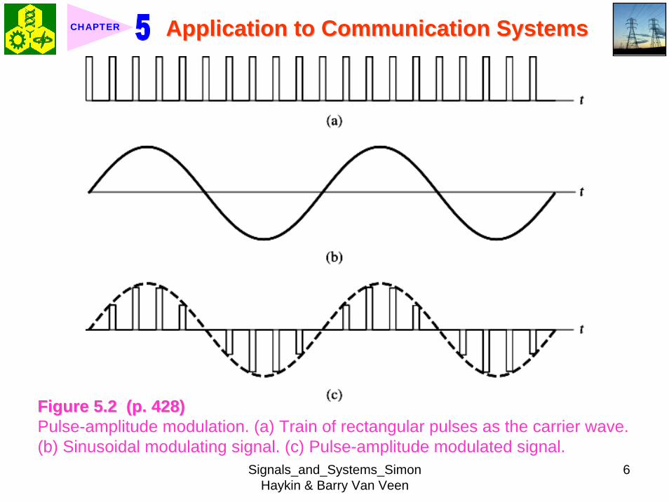
Signals_and_Systems_Simon Haykin amp Barry Van Veen
7
Application to Communication SystemsApplication to Communication SystemsCHAPTER
3 Subclasses of pulse modulation1)1) Analog pulse modulation in which a characteristic parameter sucAnalog pulse modulation in which a characteristic parameter such as the h as the
amplitude duration or position of a pulse is varied continuousamplitude duration or position of a pulse is varied continuously with the ly with the message signalmessage signal
2)2) Digital pulse modulation in which the modulated signal is repreDigital pulse modulation in which the modulated signal is represented in sented in coded formcoded form
Two operations quantization and coding
Ex PCM = Pulse-code modulation
53 53 Benefits of ModulationBenefits of Modulationclubs Four practical benefits resulting from the use of modulation1 Modulation is used to shift the spectral content of a message signal to that it
lies inside the operating frequency band of a communication channelEx Speech signal with 300 to 3100 Hz frequency components
modulationmodulation 800 ~ 900 800 ~ 900 MHz in MHz in cellular radio systemcellular radio system
1) Subband 824-849 MHz used to receive signal
2) Subband 869-894 MHz used fortransmitting signals to mobile units
Signals_and_Systems_Simon Haykin amp Barry Van Veen
8
Application to Communication SystemsApplication to Communication SystemsCHAPTER
2 Modulation provides a mechanism for putting the information content of a message signal into a form that may be less vulnerable to noise orinterference
3 Modulation permits the use of multiplexing4 Modulation makes it possible for the physical size of the transmitting or
receiving antenna to assume a practical valueclubs Detailed description See pp429 ~ 430 textbook
54 54 Full Amplitude ModulationFull Amplitude Modulation1 Sinusoidal carrier wave
( ) cos( )c cc t A tω= (57)
2 Amplitude modulation (AM) is defined as a process in which the amplitude of the carrier is varied in proportion to a message signal m(t) according to theformula
[ ]( ) 1 ( ) cos( )c a cs t A k m t tω= + (58) kkaa is the amplitude sensitivity is the amplitude sensitivity
factor of the modulatorfactor of the modulators(t) = modulated signal m(t) = message signa
541 541 Performance of ModulationPerformance of Modulation
Angle φ(t) is assumed to be zero
Signals_and_Systems_Simon Haykin amp Barry Van Veen
9
Application to Communication SystemsApplication to Communication SystemsCHAPTER
1 The envelope of the AM wave s(t)( ) 1 ( )c aa t A k m t= + (59)
2 Two cases arise depending on the magnitude of kam(t) compare with unity1) Undermodulation which is governed by the condition
[ ]( ) 1 ( ) for all tc aa t A k m t= +
( ) 1 for allak m t tle 1 + kam(t) gt 0The envelope of the AM wave is then simplified as
(510)
2) Overmodulation which is governed by the weaker condition( ) 1 for someak m t tgt
3 Percentage modulation equiv kam(t)times 100542 542 Generation of AM WaveGeneration of AM Wave1 Another form of the modulated AM wave s(t)
[ ]( ) ( ) cos( )a c cs t k m t B A tω= + (511) BB = 1= 1kkaa equivequiv a a biasbias that is added to the message signal that is added to the message signal mm((tt) before modulation) before modulation
Signals_and_Systems_Simon Haykin amp Barry Van Veen
10
Application to Communication SystemsApplication to Communication SystemsCHAPTER
2 Block diagram for generating an AM wave Fig 53Fig 53Basically it consists of two functional blocks1)1) An adder which adds the bias An adder which adds the bias BB to the incoming message signal to the incoming message signal mm((tt))2)2) A multiplier which multiplies the adder output A multiplier which multiplies the adder output ((mm((tt) + ) + BB)) by the carrier wave by the carrier wave
AAcccoscos((ωωcctt)) producing the AM wave producing the AM wave ss((tt))
Figure 53 (p 432)Figure 53 (p 432)Spectrum involving an adder and multiplier for generating an AM wave
v equiv ω p equiv π
543 543 Possible Waveforms of AM WavePossible Waveforms of AM Wave1 Fig 54Fig 54 illustrates the waveforms generated by the amplitude modulation
processPart (a) message signal Part (a) message signal mm((tt) (b) percentage modulation = 667 and (c) 1667) (b) percentage modulation = 667 and (c) 1667
Signals_and_Systems_Simon Haykin amp Barry Van Veen
11
Application to Communication SystemsApplication to Communication SystemsCHAPTER
Figure 54 (p 432)Figure 54 (p 432)Amplitude modulation for a varying percentage of modulation (a) Message signal m(t) (b) AM wave for |kam(t)| lt 1 for all t where ka is the amplitude sensitivity of the modulator This case represents undermodulation (c) AM wave for |kam(t)| gt 1 some of the time This case represents overmodulation
Signals_and_Systems_Simon Haykin amp Barry Van Veen
12
Application to Communication SystemsApplication to Communication SystemsCHAPTER
2 Important conclusionThe envelope of the AM wave has a waveform that bears a oneThe envelope of the AM wave has a waveform that bears a one--toto--one one correspondence with that of the message signal if the percentagecorrespondence with that of the message signal if the percentage modulation is modulation is less than or equal to 100less than or equal to 100
clubs If percentage modulation gt 100 the modulated wave is said to suffer fromenvelope distortion
544 544 Does FullDoes Full--Amplitude Modulation Satisfy the Linearity Property Amplitude Modulation Satisfy the Linearity Property 1 Amplitude modulation as defined in Eq (58) fails the linearity test in a
strict sense2 Demonstration
1) 1) Suppose that Suppose that mm((tt) = ) = mm11(t) + (t) + mm22((tt) Let ) Let ss11((tt) and ) and ss22((tt) denote the AM waves ) denote the AM waves produced by these two components acting separatelyproduced by these two components acting separately
2) 2) Let the operator Let the operator HH denote the amplitude modulation process therefore we denote the amplitude modulation process therefore we havehave
[ ]1 1( ) 1 ( ) cos( )c a cs t A k m t tω= + [ ]2 2( ) 1 ( ) cos( )c a cs t A k m t tω= +and
( )1 2 1 2
1 2
( ) ( ) 1 ( ) ( ) cos( )
( ) ( )c a cH m t m t A k m t m t t
s t s t
ω+ = + +⎡ ⎤⎣ ⎦ne +
Signals_and_Systems_Simon Haykin amp Barry Van Veen
13
Application to Communication SystemsApplication to Communication SystemsCHAPTER
The superposition principle is violatedThe superposition principle is violated
545 545 FrequencyFrequency--Domain Description of Amplitude ModulationDomain Description of Amplitude Modulation1 Fourier transform pairs
( ) ( )FTs t S jωlarr⎯⎯rarr and ( ) ( )FTm t M jωlarr⎯⎯rarr
Message Message spectrumspectrum
2 Fourier transform of Accos(ωct)
[ ]( ) ( )c c cAπ δ ω ω δ ω ωminus + +
cFourier transform of m(t)cos( t)ω
[ ]1 ( ) ( )2 c cM j j M j jω ω ω ωminus + +
3 Fourier transform of the AM wave of Eq (58)
[ ]
[ ]
( ) ( ) ( )1 + ( ( )) ( ( )) 2
c c c
a c c c
S j A
k A M j M j
ω π δ ω ω δ ω ω
ω ω ω ω
= minus + +
minus + +(512)
Fig 55Fig 55
Signals_and_Systems_Simon Haykin amp Barry Van Veen
14
Application to Communication SystemsApplication to Communication SystemsCHAPTER
Figure 55 (p 434)Figure 55 (p 434)Spectral content of AM wave (a) Magnitude spectrum of message signal (b) Magnitude spectrum of the AM wave showing the compositions of the carrier and the upper and lower sidebands
v equiv ω p equiv π
clubs Descriptions for Fig 55Fig 55
1)1) The message signal is band limited to the interval The message signal is band limited to the interval minusminus ωωmm lele ωω lele ωωmm2)2) ωωmm equivequiv the message bandwidth of the message bandwidth of mm((tt) in rads) in rads3)3) The spectrum of The spectrum of SS((jjωω) consists of two impulse functions weighted by the factor ) consists of two impulse functions weighted by the factor
ππAAcc and occurring at and occurring at plusmnplusmn ωωcc and two versions of the message spectrum shifted in and two versions of the message spectrum shifted in frequency by frequency by plusmnplusmn ωωcc and scaled in amplitude by (12)and scaled in amplitude by (12)kkaaAAcc
The spectrum of the AM wave as The spectrum of the AM wave as depicted in Fig 55 (b) is depicted in Fig 55 (b) is fullfull
Signals_and_Systems_Simon Haykin amp Barry Van Veen
15
Application to Communication SystemsApplication to Communication SystemsCHAPTER
4) 4) Upper sideband Upper sideband equivequiv the spectrum lying above the spectrum lying above ωωcc or below or below minusminus ωωcc5) Lower sideband 5) Lower sideband equivequiv the spectrum lying below the spectrum lying below ωωcc or above or above minusminus ωωcc
The condition ωc gt ωm is a necessary condition for the sidebands not to overlap
6) 6) Highest frequency component of the AM wave Highest frequency component of the AM wave equivequiv ωωcc + + ωωmm7) Lowest frequency component of the AM wave 7) Lowest frequency component of the AM wave equivequiv ωωcc minusminus ωωmm8) The difference between these two frequencies defines the tran8) The difference between these two frequencies defines the transmission smission
bandwidth bandwidth ωωTT for an AM wave for an AM wave
2T mω ω= (513)
Example 51 Full Amplitude Modulation for Sinusoidal Modulating SignalConsider a modulating wave m(t) that consists of a single tone or frequency component that is
0 0( ) cos( )m t A tω=
where A0 is the amplitude of the modulating wave and ω0 is its radian frequency (See Fig 56(a)Fig 56(a)) The sinusoidal carrier wave c(t) has amplitude Ac and radian frequency ωc (See Fig 56(b)Fig 56(b)) Evaluate the time-domain and frequency-domain characteristics of the AM wave
Signals_and_Systems_Simon Haykin amp Barry Van Veen
16
Application to Communication SystemsApplication to Communication SystemsCHAPTER
Figure 56 (p Figure 56 (p 435)435)Time-domain (on the left) and frequency-domain (on the right) characteristics of AM produced by a sinusoidal modulating wave (a) Modulating wave (b) Carrier wave (c) AM wave
v equiv ω p equiv π
Signals_and_Systems_Simon Haykin amp Barry Van Veen
17
Application to Communication SystemsApplication to Communication SystemsCHAPTER
ltltSolgtSolgt1 The AM wave is described by
[ ]0( ) 1 cos( ) cos( )c cs t A t tμ ω ω= + (514) where 0ak Aμ =
clubsclubs The dimensionless constant The dimensionless constant μμ for a sinusoidal modulating wave is called the for a sinusoidal modulating wave is called the modulation factormodulation factor and equals the percentage modulation when it is expressedand equals the percentage modulation when it is expressednumerically as a percentage numerically as a percentage
clubsclubs To avoid envelope distortion due to To avoid envelope distortion due to overmodulationovermodulation the modulation factor the modulation factor μμ mustmustbe kept below unitybe kept below unity
clubsclubs Figure 56(c)Figure 56(c) is a sketch of is a sketch of ss((tt) for ) for μμ less than unityless than unity2 Let Amax and Amin denote the maximum and minimum values respectively of
the envelope of the modulated wave Then form Eq(514) we get
max
min
(1 )(1 )
c
c
A AA A
μμ
+=
minusmax min
max min
A AA A
μ minus=
+
3 Expressing the product of the two cosines in Eq (514) as the sum of two sinusoidal waves one having frequency ωc + ω0 and the other havingfrequency ωc-ω0 we get
Signals_and_Systems_Simon Haykin amp Barry Van Veen
18
Application to Communication SystemsApplication to Communication SystemsCHAPTER
102
102
( ) cos( ) cos[( ) ]
cos[( ) ]
c c c c
c c
s t A t A t
A t
ω μ ω ω
μ ω ω
= + +
+ minus
4 Fourier transform of s(t)
10 02
10 02
( ) [ ( ) ( )]
[ ( ) ( )]
[ ( ) ( )]
c c c
c c c
c c c
S j A
A
A
ω π δ ω ω δ ω ω
πμ δ ω ω ω δ ω ω ω
πμ δ ω ω ω δ ω ω ω
= minus + +
+ minus minus + + +
+ minus + + + minus
Thus in ideal terms the spectrum of a full AM wave for the spThus in ideal terms the spectrum of a full AM wave for the special case of ecial case of sinusoidal modulation consists of impulse functions at sinusoidal modulation consists of impulse functions at plusmnplusmn ωωcc ωωcc plusmnplusmn ωω00 and and--ωωc c plusmnplusmn ωω 00 as depicted inas depicted in Fig 56(c)Fig 56(c)
Example 52 Average Power of Sinusoidally Modulated SignalContinuing with Example 51 investigate the effect of varying the modulation factor μ on the power content of the AM wave ltltSolgtSolgt1 In practice the AM wave s(t) is a voltage or current signal
Signals_and_Systems_Simon Haykin amp Barry Van Veen
19
Application to Communication SystemsApplication to Communication SystemsCHAPTER
2 In either case the average power delivered to a 1-ohm load resistor by s(t) is composed of three components whose values are derived from Eq (115) asfollows
1 22
1 2 281 2 28
Carrier power
Upper side- frequency power
Lower side- frequency power
c
c
c
A
A
A
μ
μ
=
=
=
3 The ratio of the total sideband power to the total power in the modulated wave is therefore equal th μ 2(2 + μ 2) which depends only on the modulationfactor μ If μ = 1 (ie if 100 modulation is used) the total power in the twoside frequencies of the resulting AM wave is only one-third of the total powerin the modulated wave
4 Figure 57Figure 57 shows the percentage of total power in both side frequencies and in the carrier plotted against the percentage modulation
Signals_and_Systems_Simon Haykin amp Barry Van Veen
20
Application to Communication SystemsApplication to Communication SystemsCHAPTER
Figure 57 (p 437)Figure 57 (p 437)Variations of carrier power and side-frequency power with percentage modulation of AM wave for the case of sinusoidal modulation
546 546 Spectral OverlapSpectral Overlap1 When ωc lt ωm the modulated signal
s(t) undergoes frequency distortiondue to spectral overlap
Fig 58Fig 58clubs Assume that S(jω) is real valued2 The spectral overlap is produced by two movements
1)1) Movement of the lower sideband into the negative frequency rangeMovement of the lower sideband into the negative frequency range2)2) Movement of the image of the lower sideband into the positive frMovement of the image of the lower sideband into the positive frequency rangeequency range
3 For avoiding the spectral overlap problem the necessary condition is
c mω ωge
Signals_and_Systems_Simon Haykin amp Barry Van Veen
21
Application to Communication SystemsApplication to Communication SystemsCHAPTER
Figure 58 (p 438)Figure 58 (p 438)Spectral overlap phenomenon in amplitude modulation The phenomenon arises when the carrier frequency ωc is less than the highest frequency component ωm of the modulating signal
v equiv ω p equiv π
547 547 Demodulation of AM WaveDemodulation of AM Wave1 The envelope detector provides a simple yet effective device for the
demodulation of a narrowband AM signal for which the percentage modulation is less than 100
clubsclubs Narrowband means that the carrier is large compared with the mesNarrowband means that the carrier is large compared with the message bandwidthsage bandwidth2 Circuit diagram of an envelope detector Fig 59Fig 59
1) 1) The diode is ideal presenting zero impedance to current flow inThe diode is ideal presenting zero impedance to current flow in the forwardthe forward--biased region and infinite impedance in the reversebiased region and infinite impedance in the reverse--biased region biased region
Signals_and_Systems_Simon Haykin amp Barry Van Veen
22
Application to Communication SystemsApplication to Communication SystemsCHAPTER
Figure 59 (p 438)Figure 59 (p 438)Envelope detector illustrated by (a) circuit diagram (b) AM wave input and (c) envelope detector output assuming ideal conditions
Signals_and_Systems_Simon Haykin amp Barry Van Veen
23
Application to Communication SystemsApplication to Communication SystemsCHAPTER
2) 2) The AM signal applied to the envelope is supplied by a voltage sThe AM signal applied to the envelope is supplied by a voltage source of ource of internal resistance internal resistance RRss
3) The load resistance 3) The load resistance RRll is large compared with the source resistance is large compared with the source resistance RRss During Duringthe charging process the time constant is effectively equathe charging process the time constant is effectively equal to l to RRssCC This time This time constant must be short compared with the carrier period 2constant must be short compared with the carrier period 2ππωωcc that is that is
2s
c
R πω
ltlt (515)
3 The discharging time constant is equal to RlCRRllCC must be large such that the capacitor discharges slowly but notmust be large such that the capacitor discharges slowly but not so so large that the capacitor voltage will not discharge at the maximlarge that the capacitor voltage will not discharge at the maximum rate um rate of change of the modulating wave ieof change of the modulating wave ie2 2
lc m
R Cπ πω ω
ltlt ltlt (516) ωm equiv message
bandwidth
clubs Output ripple can be removed by low-pass filter
Signals_and_Systems_Simon Haykin amp Barry Van Veen
24
Application to Communication SystemsApplication to Communication SystemsCHAPTER
55 55 Double SidebandDouble Sideband--Suppressed ModulationSuppressed Modulation1 In full AM carrier wave c(t) is completely independent of the message signal
m(t)
Transmission of carrier wave A waste of power
2 To overcome this shortcoming we may suppress the carrier component from the modulated wave resulting in double sideband-suppressed carrier(DSB-SC) modulation
3 DSB-SC modulated signal( ) ( ) ( ) cos( ) ( )c cs t c t m t A t m tω= = (517)
clubs This modulated signal undergoes a phase reversal whenever the messagesignal m(t) crosses zero as illustrated in Fig 510Fig 510(a)(a) Message signal Message signal (b)(b) DSBDSB--SC modulated wave resulting from multiplication of the message SC modulated wave resulting from multiplication of the message
signal by the sinusoidal carrier wave signal by the sinusoidal carrier wave
Signals_and_Systems_Simon Haykin amp Barry Van Veen
25
Application to Communication SystemsApplication to Communication SystemsCHAPTER
Figure 510 (p 440)Figure 510 (p 440)Double-sideband-suppressed carrier modulation (a) Message signal (b) DSB-SC modulated wave resulting from multiplication of the message signal by the sinusoidal carrier wave
551 551 FrequencyFrequency--Domain DescriptionDomain Description1 Fourier transform of modulated signal s(t)
1( ) [ ( ( )) ( ( ))]2 c c cS j A M j M jω ω ω ω ω= minus + + (518)
where M(jω) equiv Fourier transform of m(t) minus ωm le ω le ωmFig 511 (a) and (b)Fig 511 (a) and (b)
Signals_and_Systems_Simon Haykin amp Barry Van Veen
26
Application to Communication SystemsApplication to Communication SystemsCHAPTER
Figure 511 (p 441)Figure 511 (p 441)Spectral content of DSB-SC modulated wave (a) Magnitude spectrum of message signal (b) Magnitude spectrum of DSB-SC modulated wave consisting of upper and lower sidebands only
v equiv ω p equiv π
clubs The modulation process simply translates the spectrum of the message signal by plusmn ωc
clubs Transmission bandwidth = 2 ωm2 A device for achieving DSB-SC is called a product modulator or simply
multiplierFig 512 (a)Fig 512 (a) shows the block diagram of a product modulator
Signals_and_Systems_Simon Haykin amp Barry Van Veen
27
Application to Communication SystemsApplication to Communication SystemsCHAPTER
Figure 512 (p 441)Figure 512 (p 441)(a) Product modulator for generating the DSB-SC modulated wave (b) Coherent detector for demodulation of the DSB-SC modulated wave
v equiv ω p equiv π
552 552 Coherent DetectionCoherent Detection1 The message signal m(t) may be recovered from DSB-SC
Fig 512 (b)Fig 512 (b)ss((tt) ) timestimes locally generated sinusoidal wave = locally generated sinusoidal wave = vv((tt))vv((tt) filtered by a Low) filtered by a Low--pass filterpass filter
Local oscillator
2 The local oscillator should be exactly coherent or synchronized in both frequency and phase with the carrier wave c(t)
Signals_and_Systems_Simon Haykin amp Barry Van Veen
28
Application to Communication SystemsApplication to Communication SystemsCHAPTER
Coherent detection or synchronization demodulation3 Derivation for coherent detection
1) Local oscillator cos(ωct + φ )2) Product modulator output
( ) cos( ) ( )cos( ) cos( ) ( )
1 1cos( ) ( ) cos(2 ) ( )2 2
c
c c c
c c c
v t t s tA t t m t
A m t A t m t
ω φω ω φ
φ ω φ
= += +
= + +(519)
1 cos( ) ( )2 cA m tφ
1 cos(2 ) ( )2 c cA t m tω φ+
A scaled version of the original message signal m(t)
DSBDSB--SC modulated signal with carrier SC modulated signal with carrier frequency 2 frequency 2 ωωcc
3) Magnitude spectrum Fig 5134) To clear separate two component of v(t) the original carrier frequency ωc
must satisfy the condition
Signals_and_Systems_Simon Haykin amp Barry Van Veen
29
Application to Communication SystemsApplication to Communication SystemsCHAPTER
Figure 513 (p 442)Figure 513 (p 442)Magnitude spectrum of the product modulator output v(t) in the coherent detector of Fig 512(b)
v equiv ω p equiv π
2 c m mω ω ωminus gt c mω ωgt (520) ωωmm equivequiv message bandwidthmessage bandwidth
4 Specification of low-pass filter1) 1) The cutoff frequency must be The cutoff frequency must be ωωm m 2) The transition band must be 2) The transition band must be ωωm m ≦≦ ωω ≦≦ ωωc c ωωm m
Thus the overall output in Thus the overall output in Fig 512(b)Fig 512(b) is given byis given by1( ) cos( ) ( )2o cv t A m tφ= (521)
cosφ equiv attenuation factor
Signals_and_Systems_Simon Haykin amp Barry Van Veen
30
Application to Communication SystemsApplication to Communication SystemsCHAPTER
5 (1) Demodulated signal vo(t) is proportional to m(t) when the error phase φis a constant
(2) Demodulated signal is maximum when φ = 0 and has a minimum zero when φ = plusmn π2
Example 53 Sinusoidal DSB-SC ModulationConsider again the sinusoidal modulating signal
0 0( ) cos( )m t A tω=
( ) cos( )c cc t A tω=with amplitude A0 and frequency ω0 see Fig 514(a) The carrier wave is
with amplitude Ac and frequency ωc see Fig 514(b) Investigate the time-domain and frequency-domain characteristics of the corresponding DSB-SC modulated waveltltSolgtSolgt
clubs φ = plusmn π2 represents the quadrature null effect of the coherent detector
1 The modulated DSB-SC signal is defined by
0 0
0 0 0 0
( ) cos( ) cos( )1 1cos[( ) ] cos[( ) ]2 2
c c
c c c c
s t A A t t
A A t A A t
ω ω
ω ω ω ω
=
= + + minus
Signals_and_Systems_Simon Haykin amp Barry Van Veen
31
Application to Communication SystemsApplication to Communication SystemsCHAPTER
2 The Fourier transform of s(t) is given by
0 0 0
0 0
1( ) cos[ ( ) ( )]2
( ) ( )
c c c
c c
S j A Aω π δ ω ω ω δ ω ω ω
δ ω ω ω δ ω ω ω
= minus minus + + +
+ minus + + + minus
which consists of four weighted impulse functions at the frequencies ωc+ ω0-ωc- ω0 ωc- ω0 and- ωc+ ω0 as illustrated in the right-hand side of Fig Fig 514(c)514(c)
3 This Fourier transform differs from that depicted in the right-hand side of Fig Fig 56(c)56(c) for the corresponding example of full AM in one important respect The impulse functions at plusmn ωc due to the carrier are removed
4 Application of the sinusoidally modulated DSB-SC signal to the product modulator of Fig 512(b) yields the output (assuming φ = 0)
0 0 0
0 0 0 0 0
1( ) cos( ) cos[( ) ] cos[( ) ]21 cos[(2 ) ] cos( ) cos[(2 ) ] cos( )4
c c c c
c c c
v t A A t t t
A A t t t t
ω ω ω ω ω
ω ω ω ω ω ω
= + + minus
= + + + minus +
Signals_and_Systems_Simon Haykin amp Barry Van Veen
32
Application to Communication SystemsApplication to Communication SystemsCHAPTER
Figure 514 (p Figure 514 (p 443)443)Time-domain (on the left) and frequency-domain (on the right) characteristics of DSB-SC modulation produced by a sinusoidal modulating wave (a) Modulating wave (b) Carrier wave (c) DSB-SC modulated wave Note that ω= 2πƒ
v equiv ω p equiv π
Signals_and_Systems_Simon Haykin amp Barry Van Veen
33
Application to Communication SystemsApplication to Communication SystemsCHAPTER
5 The first two sinusoidal terms of v(t) are produced by the upper side frequency and the last two sinusoidal terms are produced by the lower side frequency
6 With ωcgt ω0 the first and third sinusoidal terms of frequencies 2ωc+ ω0 and 2ωc-ω0 respectively are removed by the low-pass filter of Fig 512(b)Fig 512(b) which leaves the second and fourth sinusoidal terms of frequency ω0 as the only output of the filter The coherent detector output thus reproduces the original modulating wave
7 Note however that this output appears as two equal terms one derived from the upper side frequency and the other from the lower side frequency We therefore conclude that for the transmission of the sinusoidal signal A0 cos(ω0t) only one side frequency is necessary (The issue will be discussed further in Section 57Section 57)
553 553 CostasCostas ReceiverReceiver1 Costas receiver Fig 515Fig 5152 This receiver consists of two coherent detector supplied with the same input
ie the incoming DSB-Sc wave
cos(2 ) ( )c cA f t m tπ but with individual local oscillator signals that are in phase duadrature with respect to each other
In-phase coherent detector (I-Channel) and quadrature-phase coherent detector (Q-Channel)
Signals_and_Systems_Simon Haykin amp Barry Van Veen
34
Application to Communication SystemsApplication to Communication SystemsCHAPTER
Figure 515 (p 445)Figure 515 (p 445)Costas receiver
v equiv ω p equiv π
Signals_and_Systems_Simon Haykin amp Barry Van Veen
35
Application to Communication SystemsApplication to Communication SystemsCHAPTER
56 56 QuadratureQuadrature--Carrier MultiplexingCarrier Multiplexing
Figure 516 (p 446)Figure 516 (p 446)Quadrature-carrier multiplexing system exploiting the quadrature null effect (a) Transmitter (b) Receiver assuming perfect synchronization with the transmitter
v equiv ω p equiv π
1 1 A A quadraturequadrature--carrier multiplexing or carrier multiplexing or quadraturequadrature--amplitude modulation (QAM) amplitude modulation (QAM) system enables two DSBsystem enables two DSB--SC modulated waves to occupy the same transmission SC modulated waves to occupy the same transmission bandwidth and yet it allows for their separation at the receivebandwidth and yet it allows for their separation at the receiver outputr output
BandwidthBandwidth--conservation schemeconservation scheme
Signals_and_Systems_Simon Haykin amp Barry Van Veen
36
Application to Communication SystemsApplication to Communication SystemsCHAPTER
2 Fig 5-16(a) Block diagram of the quadrature-carrier multiplexing systemFig 5-16(a) transmitter Fig 5-16(b) receiver
3 Multiplexed signal s(t)
(522) 1 2( ) ( ) cos( ) ( )sin( )c c c cs t A m t t A m t tω ω= +
where m1(t) and m2(t) denotes the two different message signals applied to the product modulations
clubsTransmission bandwidth = 2 ωm centered at ωc where ωm is the commonmessage bandwidth of m1(t) and m2(t)
4 The output of the top detector at receiver is 1
12 ( )cA m t
The output of the bottom detector at receiver is1
22 ( )cA m t
57 57 Other Variants of Amplitude Modulation Other Variants of Amplitude Modulation clubs Basic concept Full AM and DSB-SC rArr Wasteful of bandwidthclubs Given the amplitude and phase spectra of either lower or upper sideband
we can uniquely determine the other
Signals_and_Systems_Simon Haykin amp Barry Van Veen
37
Application to Communication SystemsApplication to Communication SystemsCHAPTER
clubs Single-sideband (SSB) modulation only one sideband is transmitted571 571 FrequencyFrequency--Domain Description of SSB ModulationDomain Description of SSB Modulation1 Consider a message signal m(t) with a spectrum M(jω) limited to the band
ωa le ω le ωb Fig 5-17 (a)2 DSB-SC modulated signal
( ) cos( )c cm t A tωtimes Fig 5-17 (b)
3 (1) Upper sideband the frequencies above ωc and below minus ωc(2) Upper sideband the frequencies below ωc and above minus ωc
Fig 5-17 (c)4 When only the lower sideband is transmitted the spectrum of the
corresponding SSB modulated wave is as shown in Fig 5-17 (d) 5 Advantages of SSB
(1) Reduced bandwidth requirement(2) Elimination of the high-power carrier waveDisadvantage od SSB(1) Cost and complexity of implementing both the transmitter and receiver
Signals_and_Systems_Simon Haykin amp Barry Van Veen
38
Application to Communication SystemsApplication to Communication SystemsCHAPTER
Figure 517 Figure 517 (p 447)(p 447)Frequency-domain characteristics of SSB modulation (a) Magnitude spectrum of message signal with energy gap from ndash ωa to ωa
(c) Magnitude spectrum of SSB modulated wave containing upper sideband only
(d) Magnitude spectrum of SSB modulated wave containing lower sideband only
(b) Magnitude spectrum of DSB-SC signal
v equiv ω p equiv π
Signals_and_Systems_Simon Haykin amp Barry Van Veen
39
Application to Communication SystemsApplication to Communication SystemsCHAPTER
6 Frequency-discrimination scheme for producing SSB modulation Fig 518clubs Bandpass filter is designed to pass the sideband selected for transmission
and suppress the remaining sidebandclubs Requirement in SSB signal the message signal applied to the product
modulator must have a energy gap in its spectrum Refer to Fig 517 (a)
Figure 518 (p 448)Figure 518 (p 448)System consisting of product modulator and bandpass filter for generating SSB modulated wave
v equiv ω p equiv π
572 572 TimeTime--Domain Description of SSB ModulationDomain Description of SSB Modulation1 Mathematical tool Hilbert transform
The Hilbert transform of a signal x(t) is defined by1 ( ) 1ˆ( ) ( )xx t d x t
t tτ τ
π τ πinfin
minusinfin= = lowast
minusint
Signals_and_Systems_Simon Haykin amp Barry Van Veen
40
Application to Communication SystemsApplication to Communication SystemsCHAPTER
The Fourier transform of 1(πt) is minus j times the signum function denoted
1 for 0sgn( ) 0 for 0
1 for 0
ωω ω
ω
+ gt⎧⎪= =⎨⎪minus lt⎩
2 Passing x(t) through a Hilbert transformer is equivalent to the combination of the following two operations in frequency domain1) Keeping X(jω)unchanged for all ω 2) Shifting areX(jω) (ie the phase spectrum of x(t)) by +90deg for negative
frequencies and minus 90deg for positive frequencies clubs Hilbert transformer = Wideband minus 90deg phase shifter 573 573 Vestigial Sideband ModulationVestigial Sideband Modulation1 When the message signal contains significant components at extremely
low frequencies the upper and lower sidebands meet at the carrier frequency
Using SSB is inappropriateUsing SSB is inappropriateEx TV signals or
wideband dataUsing VSB (Vestigial sideband) modulation is appropriateUsing VSB (Vestigial sideband) modulation is appropriate
Signals_and_Systems_Simon Haykin amp Barry Van Veen
41
Application to Communication SystemsApplication to Communication SystemsCHAPTER
2 VSB is a compromise between SSB and DSB-SC forms of modulationIn VSB modulation one sideband is passes almost completely whereas just a trace or vestige of the other sideband is retained
3 Fig 519 illustrates a VSB modulated wave s(t) in relation to the message signal m(t)
v equiv ω p equiv π
Figure 519 (p 449)Figure 519 (p 449)Spectral content of VSB modulated wave (a) Magnitude spectrum of message signal (c) Magnitude spectrum of VSB modulated wave containing a vestige of the lower sideband
clubs The lower sideband is modified into the vestigial sideband4 Transmission bandwidth of VSB modulated wave T m vω ω ω= + (523)
where ωm is the message bandwidth and ωu is the width of the vestigial sideband
Signals_and_Systems_Simon Haykin amp Barry Van Veen
42
Application to Communication SystemsApplication to Communication SystemsCHAPTER
5 Generation of VSB modulated wave Fig 520
Figure 520 (p 450)Figure 520 (p 450)System consisting of product modulator and sideband shaping filter for generating VSB modulated wave
v equiv ω p equiv π
Passing a DSBPassing a DSB--SC modulated wave through a sidebandSC modulated wave through a sideband--shaping filtershaping filter6 The sideband-shaping filter is designed so that the original message
spectrum M(jω) is reproduced on the demodulation as a result of the superposition of two spectra
1) The positive-frequency part of S(jω) (ie the Fourier transform of the transmitted signal s(t)) shifted downward in frequency by ωc
2) The negative-frequency part of S(jω) shifted upward in frequency by ωc
Fig 521 A reflection of the vestige of the lower sideband makes up for the missing parts of the upper sideband
Signals_and_Systems_Simon Haykin amp Barry Van Veen
43
Application to Communication SystemsApplication to Communication SystemsCHAPTER
Figure 521 (p 450)Figure 521 (p 450)Superposition of the two spectra shown in parts (a) and (b) of the figure results in the original message spectrum (shown dashed) upon demodulation
58 58 PulsePulse--Amplitude Modulation Amplitude Modulation clubs Basic concept
Basic role in the operation of AM Frequency-shiftingBasic role in the operation of PAM Sampling
581 581 Sampling RevisitedSampling Revisited1 Sampling theorem
In view point of PAMIn view point of PAM
Signals_and_Systems_Simon Haykin amp Barry Van Veen
44
Application to Communication SystemsApplication to Communication SystemsCHAPTER
1) A band-limited signal of finite energy that has no radian frequency components higher than ωm is uniquely determined by the values of the signal at instants of time separated by π ωm seconds
2) A band-limited signal of finite energy that has no radian frequency components higher than ωm may be completely recovered from a knowledge of its samples taken at the rate of ωm π per seconds
clubs Part 1) rArr Be exploited in the transmitter of a PAM clubs Part 2) rArr Be exploited in the Receiver of a PAM2 To combat the effects of aliasing in practice we use two corrective measures1) Prior to sampling a low-pass antialiasing filter is used to attenuate those high-
frequency components of the signal which lie outside the band of interest2) The filtered signal is sampled at a rate slightly higher than the Nyquist rate3 Generation of a PAM signal Fig 522Fig 522Example 54 Telephonic CommunicationThe highest frequency component of a speech signal needed for telephonic communication is about 31 kHz Suggest a suitable value for the sampling rate ltltSolgtSolgt
Signals_and_Systems_Simon Haykin amp Barry Van Veen
45
Application to Communication SystemsApplication to Communication SystemsCHAPTER
Figure 522 (p 451)Figure 522 (p 451)System consisting of antialiasing filter and sample-and-hold circuit for converting a message signal into a flattopped PAM signal
1 The highest frequency component of 31 kHz corresponds to 362 10 radsmω π= times
Correspondingly the Nyquist rate is
62 kHzmωπ
=
2 A suitable value for the sampling rate-one slightly higher than the Nyquistrate-may be 8 kHz a rate that is the international standard for telephone speech signals
Signals_and_Systems_Simon Haykin amp Barry Van Veen
46
Application to Communication SystemsApplication to Communication SystemsCHAPTER
582 582 Mathematical Description of PAMMathematical Description of PAM1 The carrier wave used in PAM consists of a sequence of short pulses of
fixed duration in terms of which PAM is formally defined as followsPAM is a form of pulse modulation in which the amplitude of the PAM is a form of pulse modulation in which the amplitude of the pulsed carrier is pulsed carrier is varied in accordance with instantaneous sample values of the mesvaried in accordance with instantaneous sample values of the message signalsage signal the duration of the pulsed carrier is maintained constant throughout
Fig 523Fig 523
Figure 523 (p452) Figure 523 (p452) Waveform of flattopped PAM signal with pulse duration T0 and sampling period Ts
Signals_and_Systems_Simon Haykin amp Barry Van Veen
47
Application to Communication SystemsApplication to Communication SystemsCHAPTER
2 Mathematical representation of the PAM
( ) [ ] ( )sn
s t m n b t nTinfin
=minusinfin
= minussum (524) s(t) equiv PAM signal m(t) equiv
message signal
Ts equiv sampling period m[n] equiv the values of m(t) at t = nTs h(t) equiv rectangular pulse of the unit amplitude and duration T0
3 Rectangular pulse
01 0( )
0 otherwiset T
h tlt lt⎧
= ⎨⎩
(525) Fig 524 (a)Fig 524 (a)
clubs Eq (524) is a sample-and-hold operationAnalogous to zeroAnalogous to zero--orderorder--holdhold--
based reconstruction in Sec 46based reconstruction in Sec 46
差異差異hh((tt) ) 的的TTss與與TT00
4 Impulse-sampled version of message signal m(t)
( ) [ ] ( )sn
m t m n t nTδ δinfin
=minusinfin
= minussum (526)
5 PAM signal( ) [ ] ( )
( ) ( )
sn
s t m n b t nT
m t b tδ
infin
=minusinfin
= minus
=
sum(527)
Convolution of impulse-sampled version mδ(t) and h(t)
Time domain Time domain operationoperation
Signals_and_Systems_Simon Haykin amp Barry Van Veen
48
Application to Communication SystemsApplication to Communication SystemsCHAPTER
Figure 524 (p 453)(a) Rectangular pulse h(t) of unit amplitude and duration T0 (b) Magnitude spectrum |H(jω)| and phase spectrum argH(jω) of pulse h(t)
v equiv ω p equiv π
Signals_and_Systems_Simon Haykin amp Barry Van Veen
49
Application to Communication SystemsApplication to Communication SystemsCHAPTER
6 FT of PAM signal( ) ( ) ( )S j M j H jδω ω ω= (528)
where( ) ( )FTS j s tω larr⎯rarr ( ) ( )FTM j m tδ δω larr⎯rarr ( ) ( )FTH j h tω larr⎯rarr
7 Impulse sampling of the message signal m(t) introduces periodicity into the spectrum as given by
1( ) ( ( ))sks
M j M j kTδ ω ω ω
infin
=minusinfin
= minussum (529) 1Ts equiv sampling rate ωs = 2πTs rads
1( ) ( ( )) ( )sks
S j M j k H jT
ω ω ω ωinfin
=minusinfin
= minussum (530)
( ) ( )FTM j m tω larr⎯rarrwhere
clubs Suppose that m(t) is strictly band limited and that the sampling rate 1Ts is greater than the Nyquist rate Then passing s(t) through a reconstruction filter chosen as an ideal low-pass filter with cutoff frequency ωm and gain Ts we find that the spectrum of the resulting filter output is equal to M(jω)H(jω)
Signals_and_Systems_Simon Haykin amp Barry Van Veen
50
Application to Communication SystemsApplication to Communication SystemsCHAPTER
8 From Eq (525) we find that0 2
0 0( ) sin ( (2 )) j TH j T c T e ωω ω π minus= (531) Fig 524(b) magnitude and phase of H(jω)
clubs Using PAM to represent a continuous-time message signal we introduce amplitude distortion as well as a delay of T02
clubs The frequency distortion caused by the use of flat-topped sampled in the generation of a PAM wave illustrated in Fig 523Fig 523 is referred to as the aperture effect
583 583 Demodulation of PAM SignalDemodulation of PAM Signal1 Reconstruction scheme Fig 525Fig 525
Figure 525 (p 454)Figure 525 (p 454)System consisting of low-pass interpolation filter and equalizer for reconstructing a message signal from its flattopped sampled version
clubs The system consists of low-pass interpolation filter and equalizer connected in cascade
Signals_and_Systems_Simon Haykin amp Barry Van Veen
51
Application to Communication SystemsApplication to Communication SystemsCHAPTER
2 The cutoff frequency of low-pass filter = the highest frequency ωm of message signal
3 The equalizer is used to correct the aperture effect due to flat-topped sampling in the sample-and-hold circuit
4 The equalizer has the effect of decreasing the in-band loss of the interpolation filter as frequency increases in such a manner as to compensate for the aperture effect
5 Amplitude response of equalizer
0
0 0 0 0
1 1 1| ( ) | | sinc( 2) | 2 | sin( 2) |
TH j T T T T
ωω ω ω
= =
Frequency response Eq (531)
Example 55 Equalization for PAM TransmissionThe duty cycle in a PAM signal namely T0 Ts is 10 Evaluate the peak amplification required for equalizationltltSolgtSolgt1 At ωm = π Ts which corresponds to the highest frequency component of the
message signal for a sampling rate equal to the Nyquist rate we find from Eq (531) that the magnitude response of the equalizer at ωm normalized to that at zero frequency is
Signals_and_Systems_Simon Haykin amp Barry Van Veen
52
Application to Communication SystemsApplication to Communication SystemsCHAPTER
Figure 526 (p 455)Figure 526 (p 455)Normalized equalization (to compensate for aperture effect) plotted against the duty cycle T0Ts
Signals_and_Systems_Simon Haykin amp Barry Van Veen
53
Application to Communication SystemsApplication to Communication SystemsCHAPTER
0
0 0
( 2)( )1sin (05 ) sin[( 2)( )]
s
s s
T Tc T T T T
ππ
=
where the ratio T0 Ts is equal to the duty cycle of the sampling pulses 2 In Fig 526Fig 526 this result is plotted as a function of the duty cycle T0 Ts Ideally it
should be equal to unity for all values of T0 Ts 3 For a duty cycle of 10 it is equal to 10041 It follows that for duty cycles of less
than 10 the magnitude equalization required is less than 10041 in which case the aperture effect is usually considered to be negligible
59 59 Multiplexing Multiplexing clubs Three basic types of multiplexing1 Frequency-division multiplexing in which the signals are separated by
allocating them to different frequency bands This is illustrated in Fig 527(a) for the case of six different message signals Frequency-division multiplexing favors the use of CW modulation where each message signal is able to use the channel on a continuous-time basis
2 Time-division multiplexing wherein the signals are separated by allocating them to different time slots within a sampling interval
Signals_and_Systems_Simon Haykin amp Barry Van Veen
54
Application to Communication SystemsApplication to Communication SystemsCHAPTER
This second type of multiplexing is illustrated in Fig 527(b) for the case of six different message signals Code-division multiplexing which relies on the assignment of different codes to the individual users of the channel
3 Code-division multiplexing which relies on the assignment of different codes to the individual users of the channel
591 591 FrequencyFrequency--Domain Multiplexing (FDM)Domain Multiplexing (FDM)1 Block diagram Fig 528Fig 5282 Incoming message signals low-pass variety3 Low-pass filter to remove high-frequency components such that the signal
in each channel does not disturb each other4 MOD (modulator) shift the frequency ranges of the signals so as to occupy
mutually exclusive frequency intervalsSSB is often used in this stageEx Voice input is usually assigned a bandwidth of 4 kHz
5 Band-pass filters are used to restrict the band of each modulated wave to its prescribed range
6 Band-pass filters in receiver separate the message signals7 DEM (demodulator) to recover signalsclubs FDM in Fig 528 operates in only one direction
Signals_and_Systems_Simon Haykin amp Barry Van Veen
55
Application to Communication SystemsApplication to Communication SystemsCHAPTER
Figure 527 (p 456)Figure 527 (p 456)Two basic forms of multiplexing (a) Frequency-division multiplexing (with guardbands) (b) Time-division multiplexing no provision is made here for synchronizing pulses
Signals_and_Systems_Simon Haykin amp Barry Van Veen
56
Application to Communication SystemsApplication to Communication SystemsCHAPTER
Figure 528 (p 457)Figure 528 (p 457)Block diagram of FDM system showing the important constituents of the transmitter and receiver
Signals_and_Systems_Simon Haykin amp Barry Van Veen
57
Application to Communication SystemsApplication to Communication SystemsCHAPTER
Example 56 SSB-FDM System
ltltSolgtSolgt
An FDM system is used to multiplex 24 independent voice signals SSB modulation is used for the transmission Given that each voice signal is allotted a bandwidth 4kHz calculate the overall transmission bandwidth of the channel
With each voice signal allotted a bandwidth of 4 kHz the use of SSB modulation requires a bandwidth of 4 kHz for its transmission Accordingly the overall transmission bandwidth provided by the channel is 24 X 4 = 96 kHz 592 592 TimeTime--Domain Multiplexing (TDM)Domain Multiplexing (TDM)clubs Basic to the operation of a TDM system is the sampling theoremclubs The transmission of the message samples engages the transmission channel for
only a fraction of the sampling interval on a periodic basis equal to the width T0 of a PAM modulating pulse
1 Block diagram Fig 529Fig 5292 Commutator is usually implemented by means of electronic switching
circuitry3 The function of commutator is two folds
Signals_and_Systems_Simon Haykin amp Barry Van Veen
58
Application to Communication SystemsApplication to Communication SystemsCHAPTER
Figure 529 (p 458)Figure 529 (p 458)Block diagram of TDM system showing the important constituents of the transmitter and receiver
(1) To take a narrow sample of each of the M input message signals at a rate 1Tsthat is slightly higher than ωcπ where ωc is the cutoff frequency of the input low-pass filter
(2) To sequentially interleave these M samples inside a sampling interval Ts4 Pulse modulator transform the multiplexed signal into a form suitable for
transmission over the common channel
Signals_and_Systems_Simon Haykin amp Barry Van Veen
59
Application to Communication SystemsApplication to Communication SystemsCHAPTER
clubs The use of time-division multiplexing introduces a bandwidth expansion factor M because the scheme must squeeze M samples derived from M independent message sources into a time slot equal to one sampling interval
5 Pulse demodulator performs the inverse operation of the pulse modulator6 Decommutator distributes the narrow samples produced by pulse demodulator to the appropriate low-pass reconstruction filter7 Synchronization between the timing operations of the transmitter and
receiver in a TDM system is essential for satisfactory performance of the system
Inserting an extra pulse into each sampling interval on a regular basisBandwidth expansion factor is increased to M + 1
clubs The TDM system is hghly sensitive to the dispersion in the common transmission channel
Example 57 Comparison of TDM with FDMATDM system is used to multiplex four independent voice signals using PAM Each voice signal is sampled at the rate of 8 kHz The system incorporates a synchronizing pulse train for its proper operation
Signals_and_Systems_Simon Haykin amp Barry Van Veen
60
Application to Communication SystemsApplication to Communication SystemsCHAPTER
(a) Determine the timing relationships between the synchronizing pulse train and the impulse trains used to sample the four voice signals
(b) Calculate the transmission bandwidth of the channel for the TDM system and compare the result with a corresponding FDM system using SSBmodulation
ltltSolgtSolgt(a) The sampling period is
31 125 s
8 10sT s μ= =times
In this example the number of voice signals is M = 4 Hence dividing the sampling period of 125 μs among these voice signals and the synchronizing pulse train we obtain the time slot allocated to each one of them
0 1125 25 s
5
sTTM
μ
=+
= =
Signals_and_Systems_Simon Haykin amp Barry Van Veen
61
Application to Communication SystemsApplication to Communication SystemsCHAPTER
Figure 530Figure 530 shows the timing relationships between the synchronizing pulse train and the four impulse trains used to sample the different voice signals in a single frame Each frame includes time slots of common duration T0 = 25 μs which are allocated to the pulse-modulated signals and synchronizing pulse
Figure 530 (p 459)Figure 530 (p 459)Composition of one frame of a multiplexed PAM signal incorporating four voice-signals and a synchronizing pulse
Signals_and_Systems_Simon Haykin amp Barry Van Veen
62
Application to Communication SystemsApplication to Communication SystemsCHAPTER
(b) As a consequence of the time-bandwidth product (see Section 317) there is an inverse relationship between the duration of a pulse and the bandwidth (ie cutoff frequency) of the channel needed for itstransmission Accordingly the overall transmission bandwidth of the channel is
0
21 1 MHz 40 kHz
25
TTf
T
ωπ
=
= = =
In contrast the use of an FDM system based on SSB modulation requires a channel bandwidth equal to M times that of a single voice signal-that is 4 X 4 = 16 kHz Thus the use of PAM-TDM requires a channel bandwidth that is 40 16 = 25 times that of SSB-FDMIn practice pulse-code modulation is commonly used as the method of modulation for TDM this results in a further increase in channel bandwidth depending on the length of the code word used in the digital representation of each pulse in the PAM signal
Signals_and_Systems_Simon Haykin amp Barry Van Veen
63
Application to Communication SystemsApplication to Communication SystemsCHAPTER
510 510 Pulse and Group Delays Pulse and Group Delays 1 Whenever a signal is transmitted through a dispersive (ie frequency
selective) system some delay is introduced into the output signal in relation to the input signal
2 The delay is determined by the phase response of the system3 Phase response of a dispersive communication channel
( ) arg ( )H jφ ω ω= (532)
A signal is transmitted through the channel at a frequency ωc The signal received at the channel lags the transmitted signal by φ(ωc) The time delay is called phase delay formally defined as
( )cp
c
φ ωτω
= minus (533)
The phase delay is not necessarily the true signal delayclubs Case study for DSB-SC1 Transmitted signal
0( ) cos( ) cos( )cs t A t tω ω= (534)
ωc equiv carrier frequency ω0 equiv sinusoidal modulation frequency
A = AcA0
Signals_and_Systems_Simon Haykin amp Barry Van Veen
64
Application to Communication SystemsApplication to Communication SystemsCHAPTER
1 21 1( ) cos( ) cos( )2 2
s t A t A tω ω= +
1 0cω ω ω= + (535) where
2 0cω ω ω= minus (536)
Upper frequency
Lower frequency
2 Let the s(t) be transmitted through the channel with phase response φ (ω) Accordingly the signal received at the channel output is
1 1 2 21 1( ) cos( ( )) cos( ( ))2 2
y t A t A tω φ ω ω φ ω= + + +
1 2 1 20
( ) ( ) ( )1 ( )( ) cos cos2 2cy t A t tφ ω φ ω φ ω φ ωω ω+⎛ ⎞ ⎛ ⎞= + +⎜ ⎟ ⎜ ⎟
⎝ ⎠ ⎝ ⎠(537)
3 Two observations from Eq (537)1) The carrier component at frequency ωc in y(t) lags its counterpart in s(t) by
frac12 (φ (ω1) + φ (ω2)) which represents a time delay equal to
1 2 1 2
c 1 2
( )+ ( ) ( )+ ( )2 +
φ ω φ ω φ ω φ ωω ω ω
minus = minus (538)
Signals_and_Systems_Simon Haykin amp Barry Van Veen
65
Application to Communication SystemsApplication to Communication SystemsCHAPTER
2) The message component at frequency ω0 in y(t) lags its counterpart in s(t) by frac12 (φ (ω1) minus φ (ω2)) which represents a time delay equal to
1 2 1 2
0 1 2
( ) ( ) ( ) ( )2
φ ω φ ω φ ω φ ωω ω ωminus minus
minus = minusminus
(539)
4 Suppose that ω0 lt ωc rArr the side frequencies are close together with ω c between them Such a modulated signal is said to be a narrowband signal The phase response φ (ω) in the vicinity of ω = ωc is approximated by two-term Taylor series expansion
( )( ) ( ) ( )c
c cd
d ω ω
φ ωφ ω φ ω ω ωω =
= + times minus (540)
Phase delay = ( ) c cφ ω ωminus
5 The time delay introduced by the message signal (ie he ldquoenveloperdquo of the modulated signal) is given by
( )
c
gd
d ω ω
φ ωτω =
= minus (541) The time delay τg is called the
envelope delay or group delay
Signals_and_Systems_Simon Haykin amp Barry Van Veen
66
Application to Communication SystemsApplication to Communication SystemsCHAPTER
6 When a modulated signal is transmitted through a communication channel there are two different delays to be considered1) The carrier or phase delay τp defined by Eq (533)2) The envelope or group delay τg defined by Eq (541)
clubs The group delay is the true signal delay
Example 58 Phase and Group Delays for Ban-pass Channel
ltltSolgtSolgt
The phase response of a band-pass communication channel is defined by 2 2
1( ) tan c
c
ω ωφ ωωω
minus ⎛ ⎞minus= minus ⎜ ⎟
⎝ ⎠The signal s(t) defined in Eq (534) is transmitted through this channel with
475 radscω = 0 025 radsω =andCalculate (a) the phase delay and (b) the group delay
(a) At ω = ωc φ (ωc) = 0 According to Eq (533) the phase delay τ p is zero (b) Differentiating φ (ω) with respect to ω we get
Signals_and_Systems_Simon Haykin amp Barry Van Veen
67
Application to Communication SystemsApplication to Communication SystemsCHAPTER
2 2
2 2 2 2 2
( )( )( )
c c
c c
dd
ω ω ωφ ωω ω ω ω ω
+= minus
+ minus
Using thing result in Eq (541) we find that the group delay is 2 2 04211
475gc
sτω
= = =
1 One waveform shown as a solid curve was obtained by multiplying the transmitted signal s(t) by the carrier wave cos(ωct)
2 The second waveform shown as a dotted curve was obtained by multiplying the received signal y(t) by the carrier wave cos(ωct)
To display the results obtained in parts (a) and (b) in graphical form Fig 531Fig 531shows a superposition of two waveforms obtained as follows
The figure clearly shows that the carrier (phase) delay τ p is zero and the envelope of the received signal y(t) is lagging behind that of the transmitted signal by τs seconds For the presentation of waveforms in this figure we purposely did not use a filter to suppress the high frequency components resulting from the multiplications described under points 1 and 2 because of the desire to retain a contribution due to the carrier for display
Signals_and_Systems_Simon Haykin amp Barry Van Veen
68
Application to Communication SystemsApplication to Communication SystemsCHAPTER
Figure 531 Figure 531 (p 463)(p 463)Highlighting the zero carrier delay (solid curve) and group delay τg (dotted curve) which are determined in accordance with Example 58
Signals_and_Systems_Simon Haykin amp Barry Van Veen
69
Application to Communication SystemsApplication to Communication SystemsCHAPTER
clubs Not also that the separation between the upper side frequency ω1 = ωc + ω0 = 500 rads and the lower side frequency ω2 = ωc minus ω0 = 450 rads is about 10 of the carrier frequency ωc = 475 rads which justifies referring to the modulated signal in this example as a narrowband signal
5101 5101 Some Practical ConsiderationsSome Practical Considerationsclubs What is the practical importance of group delay 1 Eq (541) for determining group delay applies strictly to narrowband
modulated signal2 The message bandwidth may be comparable to the carrier frequency In
this situation the group delay is formulated as a frequency-dependent parameter ie ( )d( )g d
φ ωτ ωω
= minus (542)
3 When a wideband modulated signals transmitted through a dispersive channel the frequency components of the message signal are delayed by different amounts at the channel output
Delay distortionFig 532Fig 532 Group delay response of voice-grade telephone channel
Signals_and_Systems_Simon Haykin amp Barry Van Veen
70
Application to Communication SystemsApplication to Communication SystemsCHAPTER
Figure 532 (p 464)Group delay response of voice-grade telephone channel (Adapted from J C Bellamy Digital Telephony Wiley 1982)
511 511 Exploring Concepts with MATLABExploring Concepts with MATLAB5111 5111 Full AMFull AMclubs Sinusoidal modulation
clubs To reconstruct a faithful version of the original message signal in the receiver we have to use a delay equalizer
0( ) [1 cos( )]cos( )c cs t A t tμ ω ω= +1 AM experiment
1cA =
08 radscω π= 0 01 radsω π=Carrier amplitude
Carrier frequency Modulation amplitude
Signals_and_Systems_Simon Haykin amp Barry Van Veen
71
Application to Communication SystemsApplication to Communication SystemsCHAPTER
2 We wish to display and analyze 10 full cycles of the AM wave corresponding to a total duration of 200 s Choosing a sampling rate 1Ts = 10 Hz we have a total of N = 2000 time samples The frequency band of interest is minus 10 π ≦ ω ≦ 10 π Since the separation between the carrier and either side frequency is equal to the modulation frequency ω0 = 01 π rads we would like to have a frequency resolution ωr = 001π rads To achieve this resolution we require the following number of frequency samples (see Eq (442))
20 2000001
s
r
M ω πω π
ge = =
3 We therefore choose M = 2000 To approximate the Fourier transform of the AM wave s(t) we may use a 2000-point DTFS The only variable in the AM experiment is the modulation factor μ with respect to which we wish to investigate three different situationsμ = 05 corresponding to under-modulationμ = 10 for which the AM system is on the verge of over-modulationμ = 20 corresponding to over-modulation
Signals_and_Systems_Simon Haykin amp Barry Van Veen
72
Application to Communication SystemsApplication to Communication SystemsCHAPTER
4 MATLAB commandsAc = 1 carrier amplitudewc = 08pi carrier frequencyw0 = 01pi modulation frequencymu = 05 modulation factort = 0011999s = Ac(1 + mucos(w0t))cos(wct)plot(ts)Smag = abs(fftshift(fft(s2000)))2000 Smag denotes the magnitude specturm of the AM wavew = 10[-1000999]2pi2000plot(wSmag)axis ([-30 30 0 08])
5 5 μμ = 05 = 05 case case Fig 533Fig 533μμ = 10 case = 10 case Fig 534Fig 534μμ = 20 case = 20 case Fig 535Fig 535
Discussion see pp 466-469 textbook
Signals_and_Systems_Simon Haykin amp Barry Van Veen
73
Application to Communication SystemsApplication to Communication SystemsCHAPTER
-30 -20 -10 0 10 20 300
02
04
06
0 50 100 150 200-2
-1
0
1
2
2 22 24 26 28 3
02
04
06
(a) Time (s)
Time domain
Frequency domain
(b) Frequency (rads)
Frequency domain
Frequency (rads)
Figure 533 (p 466)Amplitude modulation with 50 modulation (a) AM wave (b) magnitude spectrum of the AM wave and (c) expanded spectrum around the carrier frequency
μμ = 05 = 05 casecase
Signals_and_Systems_Simon Haykin amp Barry Van Veen
74
Application to Communication SystemsApplication to Communication SystemsCHAPTER
Figure 534 (p 467)Figure 534 (p 467)Amplitude modulation with 100 modulation (a) AM wave (b) magnitude spectrum of the AM wave and (c) expanded spectrum around the carrier frequency
Signals_and_Systems_Simon Haykin amp Barry Van Veen
75
Application to Communication SystemsApplication to Communication SystemsCHAPTER
Figure 535 (p 468)Amplitude modulation with 200 modulation (a) AM wave (b) magnitude spectrum of the AM wave and (c) expanded spectrum around the carrier frequency
Signals_and_Systems_Simon Haykin amp Barry Van Veen
76
Application to Communication SystemsApplication to Communication SystemsCHAPTER
5112 5112 DSBDSB--SC ModulationSC Modulation1 Sinusoidal modulation
0 0( ) cos( ) cos( )c cs t A A t tω ω=
2 MATLAB commands
Ac = 1 carrier amplitudewc = 08pi carrier frequency in radsA0 = 1 amplitude of modulating signalw0 = 01pi frequency of modulating signalt = 011999s = AcA0cos(wct)cos(w0t)plot(ts)Smag = abs(fftshift(fft(s2000)))2000w = 10[-1000999]2pi2000plot(wSmag)
3 3 DSBDSB--SC modulated waveSC modulated wave Fig 536Fig 536 Discussion see pp 466-469 textbook
4 Output of the product modulator in Fig 512 (b) with φ = 0
Signals_and_Systems_Simon Haykin amp Barry Van Veen
77
Application to Communication SystemsApplication to Communication SystemsCHAPTER
Figure 536 (p 469)DSB-SC modulation (a) DSB-SC modulated wave (b) magnitude spectrum of the modulated wave and (c) expanded spectrum around the carrier frequency
Signals_and_Systems_Simon Haykin amp Barry Van Veen
78
Application to Communication SystemsApplication to Communication SystemsCHAPTER
( ) ( ) cos( )cv t s t tω=
5 MATLAB commandsgtgt v = scos(wct)
6 Fig 537 (a) waveforms of v(t) Fig 537 (b) magnitude spectrum which readily shows that v(t) consists of the following components1) A sinusoidal component with frequency 01π rads representing the
modulating wave2) A new DSB-SC modulated wave with double carrier frequency of 16π rads
in actuality the side frequencies of this modulated wave are located at 15πand 17π rads
1) The frequency of the modulating wave lies inside the passband of the filter2) The upper and lower side frequencies of the new DSB-SC modulated wave
lie inside the stopband of the filter
Accordingly we may recover the sinusoidal modulating signal by passing v(t) through low-pass filter with the following requirements
Signals_and_Systems_Simon Haykin amp Barry Van Veen
79
Application to Communication SystemsApplication to Communication SystemsCHAPTER
Figure 537 (p 470)Coherent detection of DSB-SC modulated wave (a) and (b) Waveform and magnitude spectrum of signal produced at the output of produce modulator (c) and (d) waveform and magnitude spectrum of low-pass filter output
Signals_and_Systems_Simon Haykin amp Barry Van Veen
80
Application to Communication SystemsApplication to Communication SystemsCHAPTER
The issue of how to design a filter with these requirements will be considered in detail in Chapter 8 For the present it suffices to say that the preceding requirements can be met by using the following MATLAB commands
gtgt [ba] = butter(30025)gtgt output = filter(bav)
The first command produces s special type of filter called a Butterworth filter For the experiment considered here the filter order is 3 and its normalized cutoff frequency of 0025 is calculated as follows
Actual cutoff frequency of filter 025 radsHalf the sampling rate 10 rads
0025
ππ
=
=
The second command computes the filterrsquos output in response to the product modulator output v(t) (We will revisit the design of this filter in Chapter 8) Figure 537(c) displays the waveform of the low-pass filter output this waveform represents a sinusoidal signal of frequency 005 Hz an observation that is confirmed by using the ffr command to approximate the spectrum of the filter output The result of the computation is shown in Fig 537(d)Fig 537(d)
Signals_and_Systems_Simon Haykin amp Barry Van Veen
81
Application to Communication SystemsApplication to Communication SystemsCHAPTER
7 In Fig 538 we explore another aspect of DSB-SC modulation namely the effect of varying the modulation frequency Figure 538(a) shows five cycles of a DSB-SC modulated wave that has the same carrier frequency as that in Fig 536(a) but the modulation frequency has been reduced to 0025 Hz( ie a radian frequency of 005π) Figure 538(b) shows the magnitude spectrum of this second DSB-SC modulated wave and its zoomed-in version is shown in Fig 538(c) Comparing this latter figure with Fig 536(c) we see clearly that decreasing the modulation frequency has the effect of moving the upper and lower side frequencies closer together which is consistent with modulation theory
5113 5113 Phase and Group DelayPhase and Group Delay1 In Example 58 we studied the phase and group delays for a band-pass
channel with phase response 2 2
1( ) tan c
c
ω ωφ ωωω
minus ⎛ ⎞minus= minus ⎜ ⎟
⎝ ⎠2 At ω = ωc the phase delay is τ p = 0 and the group delay is τ s = 04211s One
of the wave forms displayed in Fig 531Fig 531 is
1( ) ( ) cos( )cx t s t tω=
Signals_and_Systems_Simon Haykin amp Barry Van Veen
82
Application to Communication SystemsApplication to Communication SystemsCHAPTER
Figure 538 (p 472)Effect of varying the modulation frequency compared with that in Fig 537 (a) and (b) Waveform and magnitude spectrum of DSB-SC modulated wave with a modulation frequency one-half that used in Fig 536 (c) expanded spectrum around the carrier frequency
Signals_and_Systems_Simon Haykin amp Barry Van Veen
83
Application to Communication SystemsApplication to Communication SystemsCHAPTER
where (see page 461)
1 2( ) [cos( ) cos( )]2As t t tω ω= +
and ω1 = ωc + ω0 and ω2 = ωc - ω0 The waveform shown in the figure as a solid curve is a plot of x1(t) The other waveform also displayed in Fig 531Fig 531 is
2
1 1 2 2
( ) ( ) cos( )
[cos( ( )) cos( ( ))]cos( )2
c
c
x t y t tA t t t
ω
ω φ ω ω φ ω ω
=
= + + +
where the angle φ (ω1) and φ (ω2) are the values of the phase response φ (ω) at ω = ω1 and ω = ω2 respectively The waveform shown as a dotted curve in the figure is a plot of x2(t)
3 The generation of x1(t) and x2(t) in MATLAB is achieved with the following commands with A2 set equal to unity
Signals_and_Systems_Simon Haykin amp Barry Van Veen
84
Application to Communication SystemsApplication to Communication SystemsCHAPTER
wc = 475w0 = 025w1 = wc + w0w2 = wc - w0t = -10 0001 10o1 = -atan((w1^2 - wc^2)(w1wc))o2 = -atan((w2^2 - wc^2)(w2wc))s = cos(w1t) + cos(w2t)y = cos(w1t + o1) + cos(w2t + o2)x1 = scos(478t)x2 = ycos(475t)plot(tx1b)hold on plot(tx2k)hold offxlabel(Time)ylabel(Amplitude)
Note that we have set (A2) = 1 for convenience of presentation The function atan in the first two commands returns the arctangent Note also that the computation of both x1 and x2 involve element-by-element multiplications ndash hence the use of period followed by an asterisk
Signals_and_Systems_Simon Haykin amp Barry Van Veen
85
Application to Communication SystemsApplication to Communication SystemsCHAPTER
Signals_and_Systems_Simon Haykin amp Barry Van Veen
86
Application to Communication SystemsApplication to Communication SystemsCHAPTER
Signals_and_Systems_Simon Haykin amp Barry Van Veen
87
Application to Communication SystemsApplication to Communication SystemsCHAPTER
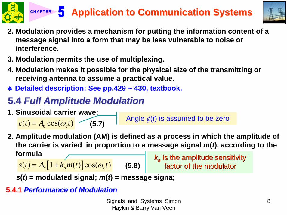
Signals_and_Systems_Simon Haykin amp Barry Van Veen
8
Application to Communication SystemsApplication to Communication SystemsCHAPTER
2 Modulation provides a mechanism for putting the information content of a message signal into a form that may be less vulnerable to noise orinterference
3 Modulation permits the use of multiplexing4 Modulation makes it possible for the physical size of the transmitting or
receiving antenna to assume a practical valueclubs Detailed description See pp429 ~ 430 textbook
54 54 Full Amplitude ModulationFull Amplitude Modulation1 Sinusoidal carrier wave
( ) cos( )c cc t A tω= (57)
2 Amplitude modulation (AM) is defined as a process in which the amplitude of the carrier is varied in proportion to a message signal m(t) according to theformula
[ ]( ) 1 ( ) cos( )c a cs t A k m t tω= + (58) kkaa is the amplitude sensitivity is the amplitude sensitivity
factor of the modulatorfactor of the modulators(t) = modulated signal m(t) = message signa
541 541 Performance of ModulationPerformance of Modulation
Angle φ(t) is assumed to be zero
Signals_and_Systems_Simon Haykin amp Barry Van Veen
9
Application to Communication SystemsApplication to Communication SystemsCHAPTER
1 The envelope of the AM wave s(t)( ) 1 ( )c aa t A k m t= + (59)
2 Two cases arise depending on the magnitude of kam(t) compare with unity1) Undermodulation which is governed by the condition
[ ]( ) 1 ( ) for all tc aa t A k m t= +
( ) 1 for allak m t tle 1 + kam(t) gt 0The envelope of the AM wave is then simplified as
(510)
2) Overmodulation which is governed by the weaker condition( ) 1 for someak m t tgt
3 Percentage modulation equiv kam(t)times 100542 542 Generation of AM WaveGeneration of AM Wave1 Another form of the modulated AM wave s(t)
[ ]( ) ( ) cos( )a c cs t k m t B A tω= + (511) BB = 1= 1kkaa equivequiv a a biasbias that is added to the message signal that is added to the message signal mm((tt) before modulation) before modulation
Signals_and_Systems_Simon Haykin amp Barry Van Veen
10
Application to Communication SystemsApplication to Communication SystemsCHAPTER
2 Block diagram for generating an AM wave Fig 53Fig 53Basically it consists of two functional blocks1)1) An adder which adds the bias An adder which adds the bias BB to the incoming message signal to the incoming message signal mm((tt))2)2) A multiplier which multiplies the adder output A multiplier which multiplies the adder output ((mm((tt) + ) + BB)) by the carrier wave by the carrier wave
AAcccoscos((ωωcctt)) producing the AM wave producing the AM wave ss((tt))
Figure 53 (p 432)Figure 53 (p 432)Spectrum involving an adder and multiplier for generating an AM wave
v equiv ω p equiv π
543 543 Possible Waveforms of AM WavePossible Waveforms of AM Wave1 Fig 54Fig 54 illustrates the waveforms generated by the amplitude modulation
processPart (a) message signal Part (a) message signal mm((tt) (b) percentage modulation = 667 and (c) 1667) (b) percentage modulation = 667 and (c) 1667
Signals_and_Systems_Simon Haykin amp Barry Van Veen
11
Application to Communication SystemsApplication to Communication SystemsCHAPTER
Figure 54 (p 432)Figure 54 (p 432)Amplitude modulation for a varying percentage of modulation (a) Message signal m(t) (b) AM wave for |kam(t)| lt 1 for all t where ka is the amplitude sensitivity of the modulator This case represents undermodulation (c) AM wave for |kam(t)| gt 1 some of the time This case represents overmodulation
Signals_and_Systems_Simon Haykin amp Barry Van Veen
12
Application to Communication SystemsApplication to Communication SystemsCHAPTER
2 Important conclusionThe envelope of the AM wave has a waveform that bears a oneThe envelope of the AM wave has a waveform that bears a one--toto--one one correspondence with that of the message signal if the percentagecorrespondence with that of the message signal if the percentage modulation is modulation is less than or equal to 100less than or equal to 100
clubs If percentage modulation gt 100 the modulated wave is said to suffer fromenvelope distortion
544 544 Does FullDoes Full--Amplitude Modulation Satisfy the Linearity Property Amplitude Modulation Satisfy the Linearity Property 1 Amplitude modulation as defined in Eq (58) fails the linearity test in a
strict sense2 Demonstration
1) 1) Suppose that Suppose that mm((tt) = ) = mm11(t) + (t) + mm22((tt) Let ) Let ss11((tt) and ) and ss22((tt) denote the AM waves ) denote the AM waves produced by these two components acting separatelyproduced by these two components acting separately
2) 2) Let the operator Let the operator HH denote the amplitude modulation process therefore we denote the amplitude modulation process therefore we havehave
[ ]1 1( ) 1 ( ) cos( )c a cs t A k m t tω= + [ ]2 2( ) 1 ( ) cos( )c a cs t A k m t tω= +and
( )1 2 1 2
1 2
( ) ( ) 1 ( ) ( ) cos( )
( ) ( )c a cH m t m t A k m t m t t
s t s t
ω+ = + +⎡ ⎤⎣ ⎦ne +
Signals_and_Systems_Simon Haykin amp Barry Van Veen
13
Application to Communication SystemsApplication to Communication SystemsCHAPTER
The superposition principle is violatedThe superposition principle is violated
545 545 FrequencyFrequency--Domain Description of Amplitude ModulationDomain Description of Amplitude Modulation1 Fourier transform pairs
( ) ( )FTs t S jωlarr⎯⎯rarr and ( ) ( )FTm t M jωlarr⎯⎯rarr
Message Message spectrumspectrum
2 Fourier transform of Accos(ωct)
[ ]( ) ( )c c cAπ δ ω ω δ ω ωminus + +
cFourier transform of m(t)cos( t)ω
[ ]1 ( ) ( )2 c cM j j M j jω ω ω ωminus + +
3 Fourier transform of the AM wave of Eq (58)
[ ]
[ ]
( ) ( ) ( )1 + ( ( )) ( ( )) 2
c c c
a c c c
S j A
k A M j M j
ω π δ ω ω δ ω ω
ω ω ω ω
= minus + +
minus + +(512)
Fig 55Fig 55
Signals_and_Systems_Simon Haykin amp Barry Van Veen
14
Application to Communication SystemsApplication to Communication SystemsCHAPTER
Figure 55 (p 434)Figure 55 (p 434)Spectral content of AM wave (a) Magnitude spectrum of message signal (b) Magnitude spectrum of the AM wave showing the compositions of the carrier and the upper and lower sidebands
v equiv ω p equiv π
clubs Descriptions for Fig 55Fig 55
1)1) The message signal is band limited to the interval The message signal is band limited to the interval minusminus ωωmm lele ωω lele ωωmm2)2) ωωmm equivequiv the message bandwidth of the message bandwidth of mm((tt) in rads) in rads3)3) The spectrum of The spectrum of SS((jjωω) consists of two impulse functions weighted by the factor ) consists of two impulse functions weighted by the factor
ππAAcc and occurring at and occurring at plusmnplusmn ωωcc and two versions of the message spectrum shifted in and two versions of the message spectrum shifted in frequency by frequency by plusmnplusmn ωωcc and scaled in amplitude by (12)and scaled in amplitude by (12)kkaaAAcc
The spectrum of the AM wave as The spectrum of the AM wave as depicted in Fig 55 (b) is depicted in Fig 55 (b) is fullfull
Signals_and_Systems_Simon Haykin amp Barry Van Veen
15
Application to Communication SystemsApplication to Communication SystemsCHAPTER
4) 4) Upper sideband Upper sideband equivequiv the spectrum lying above the spectrum lying above ωωcc or below or below minusminus ωωcc5) Lower sideband 5) Lower sideband equivequiv the spectrum lying below the spectrum lying below ωωcc or above or above minusminus ωωcc
The condition ωc gt ωm is a necessary condition for the sidebands not to overlap
6) 6) Highest frequency component of the AM wave Highest frequency component of the AM wave equivequiv ωωcc + + ωωmm7) Lowest frequency component of the AM wave 7) Lowest frequency component of the AM wave equivequiv ωωcc minusminus ωωmm8) The difference between these two frequencies defines the tran8) The difference between these two frequencies defines the transmission smission
bandwidth bandwidth ωωTT for an AM wave for an AM wave
2T mω ω= (513)
Example 51 Full Amplitude Modulation for Sinusoidal Modulating SignalConsider a modulating wave m(t) that consists of a single tone or frequency component that is
0 0( ) cos( )m t A tω=
where A0 is the amplitude of the modulating wave and ω0 is its radian frequency (See Fig 56(a)Fig 56(a)) The sinusoidal carrier wave c(t) has amplitude Ac and radian frequency ωc (See Fig 56(b)Fig 56(b)) Evaluate the time-domain and frequency-domain characteristics of the AM wave
Signals_and_Systems_Simon Haykin amp Barry Van Veen
16
Application to Communication SystemsApplication to Communication SystemsCHAPTER
Figure 56 (p Figure 56 (p 435)435)Time-domain (on the left) and frequency-domain (on the right) characteristics of AM produced by a sinusoidal modulating wave (a) Modulating wave (b) Carrier wave (c) AM wave
v equiv ω p equiv π
Signals_and_Systems_Simon Haykin amp Barry Van Veen
17
Application to Communication SystemsApplication to Communication SystemsCHAPTER
ltltSolgtSolgt1 The AM wave is described by
[ ]0( ) 1 cos( ) cos( )c cs t A t tμ ω ω= + (514) where 0ak Aμ =
clubsclubs The dimensionless constant The dimensionless constant μμ for a sinusoidal modulating wave is called the for a sinusoidal modulating wave is called the modulation factormodulation factor and equals the percentage modulation when it is expressedand equals the percentage modulation when it is expressednumerically as a percentage numerically as a percentage
clubsclubs To avoid envelope distortion due to To avoid envelope distortion due to overmodulationovermodulation the modulation factor the modulation factor μμ mustmustbe kept below unitybe kept below unity
clubsclubs Figure 56(c)Figure 56(c) is a sketch of is a sketch of ss((tt) for ) for μμ less than unityless than unity2 Let Amax and Amin denote the maximum and minimum values respectively of
the envelope of the modulated wave Then form Eq(514) we get
max
min
(1 )(1 )
c
c
A AA A
μμ
+=
minusmax min
max min
A AA A
μ minus=
+
3 Expressing the product of the two cosines in Eq (514) as the sum of two sinusoidal waves one having frequency ωc + ω0 and the other havingfrequency ωc-ω0 we get
Signals_and_Systems_Simon Haykin amp Barry Van Veen
18
Application to Communication SystemsApplication to Communication SystemsCHAPTER
102
102
( ) cos( ) cos[( ) ]
cos[( ) ]
c c c c
c c
s t A t A t
A t
ω μ ω ω
μ ω ω
= + +
+ minus
4 Fourier transform of s(t)
10 02
10 02
( ) [ ( ) ( )]
[ ( ) ( )]
[ ( ) ( )]
c c c
c c c
c c c
S j A
A
A
ω π δ ω ω δ ω ω
πμ δ ω ω ω δ ω ω ω
πμ δ ω ω ω δ ω ω ω
= minus + +
+ minus minus + + +
+ minus + + + minus
Thus in ideal terms the spectrum of a full AM wave for the spThus in ideal terms the spectrum of a full AM wave for the special case of ecial case of sinusoidal modulation consists of impulse functions at sinusoidal modulation consists of impulse functions at plusmnplusmn ωωcc ωωcc plusmnplusmn ωω00 and and--ωωc c plusmnplusmn ωω 00 as depicted inas depicted in Fig 56(c)Fig 56(c)
Example 52 Average Power of Sinusoidally Modulated SignalContinuing with Example 51 investigate the effect of varying the modulation factor μ on the power content of the AM wave ltltSolgtSolgt1 In practice the AM wave s(t) is a voltage or current signal
Signals_and_Systems_Simon Haykin amp Barry Van Veen
19
Application to Communication SystemsApplication to Communication SystemsCHAPTER
2 In either case the average power delivered to a 1-ohm load resistor by s(t) is composed of three components whose values are derived from Eq (115) asfollows
1 22
1 2 281 2 28
Carrier power
Upper side- frequency power
Lower side- frequency power
c
c
c
A
A
A
μ
μ
=
=
=
3 The ratio of the total sideband power to the total power in the modulated wave is therefore equal th μ 2(2 + μ 2) which depends only on the modulationfactor μ If μ = 1 (ie if 100 modulation is used) the total power in the twoside frequencies of the resulting AM wave is only one-third of the total powerin the modulated wave
4 Figure 57Figure 57 shows the percentage of total power in both side frequencies and in the carrier plotted against the percentage modulation
Signals_and_Systems_Simon Haykin amp Barry Van Veen
20
Application to Communication SystemsApplication to Communication SystemsCHAPTER
Figure 57 (p 437)Figure 57 (p 437)Variations of carrier power and side-frequency power with percentage modulation of AM wave for the case of sinusoidal modulation
546 546 Spectral OverlapSpectral Overlap1 When ωc lt ωm the modulated signal
s(t) undergoes frequency distortiondue to spectral overlap
Fig 58Fig 58clubs Assume that S(jω) is real valued2 The spectral overlap is produced by two movements
1)1) Movement of the lower sideband into the negative frequency rangeMovement of the lower sideband into the negative frequency range2)2) Movement of the image of the lower sideband into the positive frMovement of the image of the lower sideband into the positive frequency rangeequency range
3 For avoiding the spectral overlap problem the necessary condition is
c mω ωge
Signals_and_Systems_Simon Haykin amp Barry Van Veen
21
Application to Communication SystemsApplication to Communication SystemsCHAPTER
Figure 58 (p 438)Figure 58 (p 438)Spectral overlap phenomenon in amplitude modulation The phenomenon arises when the carrier frequency ωc is less than the highest frequency component ωm of the modulating signal
v equiv ω p equiv π
547 547 Demodulation of AM WaveDemodulation of AM Wave1 The envelope detector provides a simple yet effective device for the
demodulation of a narrowband AM signal for which the percentage modulation is less than 100
clubsclubs Narrowband means that the carrier is large compared with the mesNarrowband means that the carrier is large compared with the message bandwidthsage bandwidth2 Circuit diagram of an envelope detector Fig 59Fig 59
1) 1) The diode is ideal presenting zero impedance to current flow inThe diode is ideal presenting zero impedance to current flow in the forwardthe forward--biased region and infinite impedance in the reversebiased region and infinite impedance in the reverse--biased region biased region
Signals_and_Systems_Simon Haykin amp Barry Van Veen
22
Application to Communication SystemsApplication to Communication SystemsCHAPTER
Figure 59 (p 438)Figure 59 (p 438)Envelope detector illustrated by (a) circuit diagram (b) AM wave input and (c) envelope detector output assuming ideal conditions
Signals_and_Systems_Simon Haykin amp Barry Van Veen
23
Application to Communication SystemsApplication to Communication SystemsCHAPTER
2) 2) The AM signal applied to the envelope is supplied by a voltage sThe AM signal applied to the envelope is supplied by a voltage source of ource of internal resistance internal resistance RRss
3) The load resistance 3) The load resistance RRll is large compared with the source resistance is large compared with the source resistance RRss During Duringthe charging process the time constant is effectively equathe charging process the time constant is effectively equal to l to RRssCC This time This time constant must be short compared with the carrier period 2constant must be short compared with the carrier period 2ππωωcc that is that is
2s
c
R πω
ltlt (515)
3 The discharging time constant is equal to RlCRRllCC must be large such that the capacitor discharges slowly but notmust be large such that the capacitor discharges slowly but not so so large that the capacitor voltage will not discharge at the maximlarge that the capacitor voltage will not discharge at the maximum rate um rate of change of the modulating wave ieof change of the modulating wave ie2 2
lc m
R Cπ πω ω
ltlt ltlt (516) ωm equiv message
bandwidth
clubs Output ripple can be removed by low-pass filter
Signals_and_Systems_Simon Haykin amp Barry Van Veen
24
Application to Communication SystemsApplication to Communication SystemsCHAPTER
55 55 Double SidebandDouble Sideband--Suppressed ModulationSuppressed Modulation1 In full AM carrier wave c(t) is completely independent of the message signal
m(t)
Transmission of carrier wave A waste of power
2 To overcome this shortcoming we may suppress the carrier component from the modulated wave resulting in double sideband-suppressed carrier(DSB-SC) modulation
3 DSB-SC modulated signal( ) ( ) ( ) cos( ) ( )c cs t c t m t A t m tω= = (517)
clubs This modulated signal undergoes a phase reversal whenever the messagesignal m(t) crosses zero as illustrated in Fig 510Fig 510(a)(a) Message signal Message signal (b)(b) DSBDSB--SC modulated wave resulting from multiplication of the message SC modulated wave resulting from multiplication of the message
signal by the sinusoidal carrier wave signal by the sinusoidal carrier wave
Signals_and_Systems_Simon Haykin amp Barry Van Veen
25
Application to Communication SystemsApplication to Communication SystemsCHAPTER
Figure 510 (p 440)Figure 510 (p 440)Double-sideband-suppressed carrier modulation (a) Message signal (b) DSB-SC modulated wave resulting from multiplication of the message signal by the sinusoidal carrier wave
551 551 FrequencyFrequency--Domain DescriptionDomain Description1 Fourier transform of modulated signal s(t)
1( ) [ ( ( )) ( ( ))]2 c c cS j A M j M jω ω ω ω ω= minus + + (518)
where M(jω) equiv Fourier transform of m(t) minus ωm le ω le ωmFig 511 (a) and (b)Fig 511 (a) and (b)
Signals_and_Systems_Simon Haykin amp Barry Van Veen
26
Application to Communication SystemsApplication to Communication SystemsCHAPTER
Figure 511 (p 441)Figure 511 (p 441)Spectral content of DSB-SC modulated wave (a) Magnitude spectrum of message signal (b) Magnitude spectrum of DSB-SC modulated wave consisting of upper and lower sidebands only
v equiv ω p equiv π
clubs The modulation process simply translates the spectrum of the message signal by plusmn ωc
clubs Transmission bandwidth = 2 ωm2 A device for achieving DSB-SC is called a product modulator or simply
multiplierFig 512 (a)Fig 512 (a) shows the block diagram of a product modulator
Signals_and_Systems_Simon Haykin amp Barry Van Veen
27
Application to Communication SystemsApplication to Communication SystemsCHAPTER
Figure 512 (p 441)Figure 512 (p 441)(a) Product modulator for generating the DSB-SC modulated wave (b) Coherent detector for demodulation of the DSB-SC modulated wave
v equiv ω p equiv π
552 552 Coherent DetectionCoherent Detection1 The message signal m(t) may be recovered from DSB-SC
Fig 512 (b)Fig 512 (b)ss((tt) ) timestimes locally generated sinusoidal wave = locally generated sinusoidal wave = vv((tt))vv((tt) filtered by a Low) filtered by a Low--pass filterpass filter
Local oscillator
2 The local oscillator should be exactly coherent or synchronized in both frequency and phase with the carrier wave c(t)
Signals_and_Systems_Simon Haykin amp Barry Van Veen
28
Application to Communication SystemsApplication to Communication SystemsCHAPTER
Coherent detection or synchronization demodulation3 Derivation for coherent detection
1) Local oscillator cos(ωct + φ )2) Product modulator output
( ) cos( ) ( )cos( ) cos( ) ( )
1 1cos( ) ( ) cos(2 ) ( )2 2
c
c c c
c c c
v t t s tA t t m t
A m t A t m t
ω φω ω φ
φ ω φ
= += +
= + +(519)
1 cos( ) ( )2 cA m tφ
1 cos(2 ) ( )2 c cA t m tω φ+
A scaled version of the original message signal m(t)
DSBDSB--SC modulated signal with carrier SC modulated signal with carrier frequency 2 frequency 2 ωωcc
3) Magnitude spectrum Fig 5134) To clear separate two component of v(t) the original carrier frequency ωc
must satisfy the condition
Signals_and_Systems_Simon Haykin amp Barry Van Veen
29
Application to Communication SystemsApplication to Communication SystemsCHAPTER
Figure 513 (p 442)Figure 513 (p 442)Magnitude spectrum of the product modulator output v(t) in the coherent detector of Fig 512(b)
v equiv ω p equiv π
2 c m mω ω ωminus gt c mω ωgt (520) ωωmm equivequiv message bandwidthmessage bandwidth
4 Specification of low-pass filter1) 1) The cutoff frequency must be The cutoff frequency must be ωωm m 2) The transition band must be 2) The transition band must be ωωm m ≦≦ ωω ≦≦ ωωc c ωωm m
Thus the overall output in Thus the overall output in Fig 512(b)Fig 512(b) is given byis given by1( ) cos( ) ( )2o cv t A m tφ= (521)
cosφ equiv attenuation factor
Signals_and_Systems_Simon Haykin amp Barry Van Veen
30
Application to Communication SystemsApplication to Communication SystemsCHAPTER
5 (1) Demodulated signal vo(t) is proportional to m(t) when the error phase φis a constant
(2) Demodulated signal is maximum when φ = 0 and has a minimum zero when φ = plusmn π2
Example 53 Sinusoidal DSB-SC ModulationConsider again the sinusoidal modulating signal
0 0( ) cos( )m t A tω=
( ) cos( )c cc t A tω=with amplitude A0 and frequency ω0 see Fig 514(a) The carrier wave is
with amplitude Ac and frequency ωc see Fig 514(b) Investigate the time-domain and frequency-domain characteristics of the corresponding DSB-SC modulated waveltltSolgtSolgt
clubs φ = plusmn π2 represents the quadrature null effect of the coherent detector
1 The modulated DSB-SC signal is defined by
0 0
0 0 0 0
( ) cos( ) cos( )1 1cos[( ) ] cos[( ) ]2 2
c c
c c c c
s t A A t t
A A t A A t
ω ω
ω ω ω ω
=
= + + minus
Signals_and_Systems_Simon Haykin amp Barry Van Veen
31
Application to Communication SystemsApplication to Communication SystemsCHAPTER
2 The Fourier transform of s(t) is given by
0 0 0
0 0
1( ) cos[ ( ) ( )]2
( ) ( )
c c c
c c
S j A Aω π δ ω ω ω δ ω ω ω
δ ω ω ω δ ω ω ω
= minus minus + + +
+ minus + + + minus
which consists of four weighted impulse functions at the frequencies ωc+ ω0-ωc- ω0 ωc- ω0 and- ωc+ ω0 as illustrated in the right-hand side of Fig Fig 514(c)514(c)
3 This Fourier transform differs from that depicted in the right-hand side of Fig Fig 56(c)56(c) for the corresponding example of full AM in one important respect The impulse functions at plusmn ωc due to the carrier are removed
4 Application of the sinusoidally modulated DSB-SC signal to the product modulator of Fig 512(b) yields the output (assuming φ = 0)
0 0 0
0 0 0 0 0
1( ) cos( ) cos[( ) ] cos[( ) ]21 cos[(2 ) ] cos( ) cos[(2 ) ] cos( )4
c c c c
c c c
v t A A t t t
A A t t t t
ω ω ω ω ω
ω ω ω ω ω ω
= + + minus
= + + + minus +
Signals_and_Systems_Simon Haykin amp Barry Van Veen
32
Application to Communication SystemsApplication to Communication SystemsCHAPTER
Figure 514 (p Figure 514 (p 443)443)Time-domain (on the left) and frequency-domain (on the right) characteristics of DSB-SC modulation produced by a sinusoidal modulating wave (a) Modulating wave (b) Carrier wave (c) DSB-SC modulated wave Note that ω= 2πƒ
v equiv ω p equiv π
Signals_and_Systems_Simon Haykin amp Barry Van Veen
33
Application to Communication SystemsApplication to Communication SystemsCHAPTER
5 The first two sinusoidal terms of v(t) are produced by the upper side frequency and the last two sinusoidal terms are produced by the lower side frequency
6 With ωcgt ω0 the first and third sinusoidal terms of frequencies 2ωc+ ω0 and 2ωc-ω0 respectively are removed by the low-pass filter of Fig 512(b)Fig 512(b) which leaves the second and fourth sinusoidal terms of frequency ω0 as the only output of the filter The coherent detector output thus reproduces the original modulating wave
7 Note however that this output appears as two equal terms one derived from the upper side frequency and the other from the lower side frequency We therefore conclude that for the transmission of the sinusoidal signal A0 cos(ω0t) only one side frequency is necessary (The issue will be discussed further in Section 57Section 57)
553 553 CostasCostas ReceiverReceiver1 Costas receiver Fig 515Fig 5152 This receiver consists of two coherent detector supplied with the same input
ie the incoming DSB-Sc wave
cos(2 ) ( )c cA f t m tπ but with individual local oscillator signals that are in phase duadrature with respect to each other
In-phase coherent detector (I-Channel) and quadrature-phase coherent detector (Q-Channel)
Signals_and_Systems_Simon Haykin amp Barry Van Veen
34
Application to Communication SystemsApplication to Communication SystemsCHAPTER
Figure 515 (p 445)Figure 515 (p 445)Costas receiver
v equiv ω p equiv π
Signals_and_Systems_Simon Haykin amp Barry Van Veen
35
Application to Communication SystemsApplication to Communication SystemsCHAPTER
56 56 QuadratureQuadrature--Carrier MultiplexingCarrier Multiplexing
Figure 516 (p 446)Figure 516 (p 446)Quadrature-carrier multiplexing system exploiting the quadrature null effect (a) Transmitter (b) Receiver assuming perfect synchronization with the transmitter
v equiv ω p equiv π
1 1 A A quadraturequadrature--carrier multiplexing or carrier multiplexing or quadraturequadrature--amplitude modulation (QAM) amplitude modulation (QAM) system enables two DSBsystem enables two DSB--SC modulated waves to occupy the same transmission SC modulated waves to occupy the same transmission bandwidth and yet it allows for their separation at the receivebandwidth and yet it allows for their separation at the receiver outputr output
BandwidthBandwidth--conservation schemeconservation scheme
Signals_and_Systems_Simon Haykin amp Barry Van Veen
36
Application to Communication SystemsApplication to Communication SystemsCHAPTER
2 Fig 5-16(a) Block diagram of the quadrature-carrier multiplexing systemFig 5-16(a) transmitter Fig 5-16(b) receiver
3 Multiplexed signal s(t)
(522) 1 2( ) ( ) cos( ) ( )sin( )c c c cs t A m t t A m t tω ω= +
where m1(t) and m2(t) denotes the two different message signals applied to the product modulations
clubsTransmission bandwidth = 2 ωm centered at ωc where ωm is the commonmessage bandwidth of m1(t) and m2(t)
4 The output of the top detector at receiver is 1
12 ( )cA m t
The output of the bottom detector at receiver is1
22 ( )cA m t
57 57 Other Variants of Amplitude Modulation Other Variants of Amplitude Modulation clubs Basic concept Full AM and DSB-SC rArr Wasteful of bandwidthclubs Given the amplitude and phase spectra of either lower or upper sideband
we can uniquely determine the other
Signals_and_Systems_Simon Haykin amp Barry Van Veen
37
Application to Communication SystemsApplication to Communication SystemsCHAPTER
clubs Single-sideband (SSB) modulation only one sideband is transmitted571 571 FrequencyFrequency--Domain Description of SSB ModulationDomain Description of SSB Modulation1 Consider a message signal m(t) with a spectrum M(jω) limited to the band
ωa le ω le ωb Fig 5-17 (a)2 DSB-SC modulated signal
( ) cos( )c cm t A tωtimes Fig 5-17 (b)
3 (1) Upper sideband the frequencies above ωc and below minus ωc(2) Upper sideband the frequencies below ωc and above minus ωc
Fig 5-17 (c)4 When only the lower sideband is transmitted the spectrum of the
corresponding SSB modulated wave is as shown in Fig 5-17 (d) 5 Advantages of SSB
(1) Reduced bandwidth requirement(2) Elimination of the high-power carrier waveDisadvantage od SSB(1) Cost and complexity of implementing both the transmitter and receiver
Signals_and_Systems_Simon Haykin amp Barry Van Veen
38
Application to Communication SystemsApplication to Communication SystemsCHAPTER
Figure 517 Figure 517 (p 447)(p 447)Frequency-domain characteristics of SSB modulation (a) Magnitude spectrum of message signal with energy gap from ndash ωa to ωa
(c) Magnitude spectrum of SSB modulated wave containing upper sideband only
(d) Magnitude spectrum of SSB modulated wave containing lower sideband only
(b) Magnitude spectrum of DSB-SC signal
v equiv ω p equiv π
Signals_and_Systems_Simon Haykin amp Barry Van Veen
39
Application to Communication SystemsApplication to Communication SystemsCHAPTER
6 Frequency-discrimination scheme for producing SSB modulation Fig 518clubs Bandpass filter is designed to pass the sideband selected for transmission
and suppress the remaining sidebandclubs Requirement in SSB signal the message signal applied to the product
modulator must have a energy gap in its spectrum Refer to Fig 517 (a)
Figure 518 (p 448)Figure 518 (p 448)System consisting of product modulator and bandpass filter for generating SSB modulated wave
v equiv ω p equiv π
572 572 TimeTime--Domain Description of SSB ModulationDomain Description of SSB Modulation1 Mathematical tool Hilbert transform
The Hilbert transform of a signal x(t) is defined by1 ( ) 1ˆ( ) ( )xx t d x t
t tτ τ
π τ πinfin
minusinfin= = lowast
minusint
Signals_and_Systems_Simon Haykin amp Barry Van Veen
40
Application to Communication SystemsApplication to Communication SystemsCHAPTER
The Fourier transform of 1(πt) is minus j times the signum function denoted
1 for 0sgn( ) 0 for 0
1 for 0
ωω ω
ω
+ gt⎧⎪= =⎨⎪minus lt⎩
2 Passing x(t) through a Hilbert transformer is equivalent to the combination of the following two operations in frequency domain1) Keeping X(jω)unchanged for all ω 2) Shifting areX(jω) (ie the phase spectrum of x(t)) by +90deg for negative
frequencies and minus 90deg for positive frequencies clubs Hilbert transformer = Wideband minus 90deg phase shifter 573 573 Vestigial Sideband ModulationVestigial Sideband Modulation1 When the message signal contains significant components at extremely
low frequencies the upper and lower sidebands meet at the carrier frequency
Using SSB is inappropriateUsing SSB is inappropriateEx TV signals or
wideband dataUsing VSB (Vestigial sideband) modulation is appropriateUsing VSB (Vestigial sideband) modulation is appropriate
Signals_and_Systems_Simon Haykin amp Barry Van Veen
41
Application to Communication SystemsApplication to Communication SystemsCHAPTER
2 VSB is a compromise between SSB and DSB-SC forms of modulationIn VSB modulation one sideband is passes almost completely whereas just a trace or vestige of the other sideband is retained
3 Fig 519 illustrates a VSB modulated wave s(t) in relation to the message signal m(t)
v equiv ω p equiv π
Figure 519 (p 449)Figure 519 (p 449)Spectral content of VSB modulated wave (a) Magnitude spectrum of message signal (c) Magnitude spectrum of VSB modulated wave containing a vestige of the lower sideband
clubs The lower sideband is modified into the vestigial sideband4 Transmission bandwidth of VSB modulated wave T m vω ω ω= + (523)
where ωm is the message bandwidth and ωu is the width of the vestigial sideband
Signals_and_Systems_Simon Haykin amp Barry Van Veen
42
Application to Communication SystemsApplication to Communication SystemsCHAPTER
5 Generation of VSB modulated wave Fig 520
Figure 520 (p 450)Figure 520 (p 450)System consisting of product modulator and sideband shaping filter for generating VSB modulated wave
v equiv ω p equiv π
Passing a DSBPassing a DSB--SC modulated wave through a sidebandSC modulated wave through a sideband--shaping filtershaping filter6 The sideband-shaping filter is designed so that the original message
spectrum M(jω) is reproduced on the demodulation as a result of the superposition of two spectra
1) The positive-frequency part of S(jω) (ie the Fourier transform of the transmitted signal s(t)) shifted downward in frequency by ωc
2) The negative-frequency part of S(jω) shifted upward in frequency by ωc
Fig 521 A reflection of the vestige of the lower sideband makes up for the missing parts of the upper sideband
Signals_and_Systems_Simon Haykin amp Barry Van Veen
43
Application to Communication SystemsApplication to Communication SystemsCHAPTER
Figure 521 (p 450)Figure 521 (p 450)Superposition of the two spectra shown in parts (a) and (b) of the figure results in the original message spectrum (shown dashed) upon demodulation
58 58 PulsePulse--Amplitude Modulation Amplitude Modulation clubs Basic concept
Basic role in the operation of AM Frequency-shiftingBasic role in the operation of PAM Sampling
581 581 Sampling RevisitedSampling Revisited1 Sampling theorem
In view point of PAMIn view point of PAM
Signals_and_Systems_Simon Haykin amp Barry Van Veen
44
Application to Communication SystemsApplication to Communication SystemsCHAPTER
1) A band-limited signal of finite energy that has no radian frequency components higher than ωm is uniquely determined by the values of the signal at instants of time separated by π ωm seconds
2) A band-limited signal of finite energy that has no radian frequency components higher than ωm may be completely recovered from a knowledge of its samples taken at the rate of ωm π per seconds
clubs Part 1) rArr Be exploited in the transmitter of a PAM clubs Part 2) rArr Be exploited in the Receiver of a PAM2 To combat the effects of aliasing in practice we use two corrective measures1) Prior to sampling a low-pass antialiasing filter is used to attenuate those high-
frequency components of the signal which lie outside the band of interest2) The filtered signal is sampled at a rate slightly higher than the Nyquist rate3 Generation of a PAM signal Fig 522Fig 522Example 54 Telephonic CommunicationThe highest frequency component of a speech signal needed for telephonic communication is about 31 kHz Suggest a suitable value for the sampling rate ltltSolgtSolgt
Signals_and_Systems_Simon Haykin amp Barry Van Veen
45
Application to Communication SystemsApplication to Communication SystemsCHAPTER
Figure 522 (p 451)Figure 522 (p 451)System consisting of antialiasing filter and sample-and-hold circuit for converting a message signal into a flattopped PAM signal
1 The highest frequency component of 31 kHz corresponds to 362 10 radsmω π= times
Correspondingly the Nyquist rate is
62 kHzmωπ
=
2 A suitable value for the sampling rate-one slightly higher than the Nyquistrate-may be 8 kHz a rate that is the international standard for telephone speech signals
Signals_and_Systems_Simon Haykin amp Barry Van Veen
46
Application to Communication SystemsApplication to Communication SystemsCHAPTER
582 582 Mathematical Description of PAMMathematical Description of PAM1 The carrier wave used in PAM consists of a sequence of short pulses of
fixed duration in terms of which PAM is formally defined as followsPAM is a form of pulse modulation in which the amplitude of the PAM is a form of pulse modulation in which the amplitude of the pulsed carrier is pulsed carrier is varied in accordance with instantaneous sample values of the mesvaried in accordance with instantaneous sample values of the message signalsage signal the duration of the pulsed carrier is maintained constant throughout
Fig 523Fig 523
Figure 523 (p452) Figure 523 (p452) Waveform of flattopped PAM signal with pulse duration T0 and sampling period Ts
Signals_and_Systems_Simon Haykin amp Barry Van Veen
47
Application to Communication SystemsApplication to Communication SystemsCHAPTER
2 Mathematical representation of the PAM
( ) [ ] ( )sn
s t m n b t nTinfin
=minusinfin
= minussum (524) s(t) equiv PAM signal m(t) equiv
message signal
Ts equiv sampling period m[n] equiv the values of m(t) at t = nTs h(t) equiv rectangular pulse of the unit amplitude and duration T0
3 Rectangular pulse
01 0( )
0 otherwiset T
h tlt lt⎧
= ⎨⎩
(525) Fig 524 (a)Fig 524 (a)
clubs Eq (524) is a sample-and-hold operationAnalogous to zeroAnalogous to zero--orderorder--holdhold--
based reconstruction in Sec 46based reconstruction in Sec 46
差異差異hh((tt) ) 的的TTss與與TT00
4 Impulse-sampled version of message signal m(t)
( ) [ ] ( )sn
m t m n t nTδ δinfin
=minusinfin
= minussum (526)
5 PAM signal( ) [ ] ( )
( ) ( )
sn
s t m n b t nT
m t b tδ
infin
=minusinfin
= minus
=
sum(527)
Convolution of impulse-sampled version mδ(t) and h(t)
Time domain Time domain operationoperation
Signals_and_Systems_Simon Haykin amp Barry Van Veen
48
Application to Communication SystemsApplication to Communication SystemsCHAPTER
Figure 524 (p 453)(a) Rectangular pulse h(t) of unit amplitude and duration T0 (b) Magnitude spectrum |H(jω)| and phase spectrum argH(jω) of pulse h(t)
v equiv ω p equiv π
Signals_and_Systems_Simon Haykin amp Barry Van Veen
49
Application to Communication SystemsApplication to Communication SystemsCHAPTER
6 FT of PAM signal( ) ( ) ( )S j M j H jδω ω ω= (528)
where( ) ( )FTS j s tω larr⎯rarr ( ) ( )FTM j m tδ δω larr⎯rarr ( ) ( )FTH j h tω larr⎯rarr
7 Impulse sampling of the message signal m(t) introduces periodicity into the spectrum as given by
1( ) ( ( ))sks
M j M j kTδ ω ω ω
infin
=minusinfin
= minussum (529) 1Ts equiv sampling rate ωs = 2πTs rads
1( ) ( ( )) ( )sks
S j M j k H jT
ω ω ω ωinfin
=minusinfin
= minussum (530)
( ) ( )FTM j m tω larr⎯rarrwhere
clubs Suppose that m(t) is strictly band limited and that the sampling rate 1Ts is greater than the Nyquist rate Then passing s(t) through a reconstruction filter chosen as an ideal low-pass filter with cutoff frequency ωm and gain Ts we find that the spectrum of the resulting filter output is equal to M(jω)H(jω)
Signals_and_Systems_Simon Haykin amp Barry Van Veen
50
Application to Communication SystemsApplication to Communication SystemsCHAPTER
8 From Eq (525) we find that0 2
0 0( ) sin ( (2 )) j TH j T c T e ωω ω π minus= (531) Fig 524(b) magnitude and phase of H(jω)
clubs Using PAM to represent a continuous-time message signal we introduce amplitude distortion as well as a delay of T02
clubs The frequency distortion caused by the use of flat-topped sampled in the generation of a PAM wave illustrated in Fig 523Fig 523 is referred to as the aperture effect
583 583 Demodulation of PAM SignalDemodulation of PAM Signal1 Reconstruction scheme Fig 525Fig 525
Figure 525 (p 454)Figure 525 (p 454)System consisting of low-pass interpolation filter and equalizer for reconstructing a message signal from its flattopped sampled version
clubs The system consists of low-pass interpolation filter and equalizer connected in cascade
Signals_and_Systems_Simon Haykin amp Barry Van Veen
51
Application to Communication SystemsApplication to Communication SystemsCHAPTER
2 The cutoff frequency of low-pass filter = the highest frequency ωm of message signal
3 The equalizer is used to correct the aperture effect due to flat-topped sampling in the sample-and-hold circuit
4 The equalizer has the effect of decreasing the in-band loss of the interpolation filter as frequency increases in such a manner as to compensate for the aperture effect
5 Amplitude response of equalizer
0
0 0 0 0
1 1 1| ( ) | | sinc( 2) | 2 | sin( 2) |
TH j T T T T
ωω ω ω
= =
Frequency response Eq (531)
Example 55 Equalization for PAM TransmissionThe duty cycle in a PAM signal namely T0 Ts is 10 Evaluate the peak amplification required for equalizationltltSolgtSolgt1 At ωm = π Ts which corresponds to the highest frequency component of the
message signal for a sampling rate equal to the Nyquist rate we find from Eq (531) that the magnitude response of the equalizer at ωm normalized to that at zero frequency is
Signals_and_Systems_Simon Haykin amp Barry Van Veen
52
Application to Communication SystemsApplication to Communication SystemsCHAPTER
Figure 526 (p 455)Figure 526 (p 455)Normalized equalization (to compensate for aperture effect) plotted against the duty cycle T0Ts
Signals_and_Systems_Simon Haykin amp Barry Van Veen
53
Application to Communication SystemsApplication to Communication SystemsCHAPTER
0
0 0
( 2)( )1sin (05 ) sin[( 2)( )]
s
s s
T Tc T T T T
ππ
=
where the ratio T0 Ts is equal to the duty cycle of the sampling pulses 2 In Fig 526Fig 526 this result is plotted as a function of the duty cycle T0 Ts Ideally it
should be equal to unity for all values of T0 Ts 3 For a duty cycle of 10 it is equal to 10041 It follows that for duty cycles of less
than 10 the magnitude equalization required is less than 10041 in which case the aperture effect is usually considered to be negligible
59 59 Multiplexing Multiplexing clubs Three basic types of multiplexing1 Frequency-division multiplexing in which the signals are separated by
allocating them to different frequency bands This is illustrated in Fig 527(a) for the case of six different message signals Frequency-division multiplexing favors the use of CW modulation where each message signal is able to use the channel on a continuous-time basis
2 Time-division multiplexing wherein the signals are separated by allocating them to different time slots within a sampling interval
Signals_and_Systems_Simon Haykin amp Barry Van Veen
54
Application to Communication SystemsApplication to Communication SystemsCHAPTER
This second type of multiplexing is illustrated in Fig 527(b) for the case of six different message signals Code-division multiplexing which relies on the assignment of different codes to the individual users of the channel
3 Code-division multiplexing which relies on the assignment of different codes to the individual users of the channel
591 591 FrequencyFrequency--Domain Multiplexing (FDM)Domain Multiplexing (FDM)1 Block diagram Fig 528Fig 5282 Incoming message signals low-pass variety3 Low-pass filter to remove high-frequency components such that the signal
in each channel does not disturb each other4 MOD (modulator) shift the frequency ranges of the signals so as to occupy
mutually exclusive frequency intervalsSSB is often used in this stageEx Voice input is usually assigned a bandwidth of 4 kHz
5 Band-pass filters are used to restrict the band of each modulated wave to its prescribed range
6 Band-pass filters in receiver separate the message signals7 DEM (demodulator) to recover signalsclubs FDM in Fig 528 operates in only one direction
Signals_and_Systems_Simon Haykin amp Barry Van Veen
55
Application to Communication SystemsApplication to Communication SystemsCHAPTER
Figure 527 (p 456)Figure 527 (p 456)Two basic forms of multiplexing (a) Frequency-division multiplexing (with guardbands) (b) Time-division multiplexing no provision is made here for synchronizing pulses
Signals_and_Systems_Simon Haykin amp Barry Van Veen
56
Application to Communication SystemsApplication to Communication SystemsCHAPTER
Figure 528 (p 457)Figure 528 (p 457)Block diagram of FDM system showing the important constituents of the transmitter and receiver
Signals_and_Systems_Simon Haykin amp Barry Van Veen
57
Application to Communication SystemsApplication to Communication SystemsCHAPTER
Example 56 SSB-FDM System
ltltSolgtSolgt
An FDM system is used to multiplex 24 independent voice signals SSB modulation is used for the transmission Given that each voice signal is allotted a bandwidth 4kHz calculate the overall transmission bandwidth of the channel
With each voice signal allotted a bandwidth of 4 kHz the use of SSB modulation requires a bandwidth of 4 kHz for its transmission Accordingly the overall transmission bandwidth provided by the channel is 24 X 4 = 96 kHz 592 592 TimeTime--Domain Multiplexing (TDM)Domain Multiplexing (TDM)clubs Basic to the operation of a TDM system is the sampling theoremclubs The transmission of the message samples engages the transmission channel for
only a fraction of the sampling interval on a periodic basis equal to the width T0 of a PAM modulating pulse
1 Block diagram Fig 529Fig 5292 Commutator is usually implemented by means of electronic switching
circuitry3 The function of commutator is two folds
Signals_and_Systems_Simon Haykin amp Barry Van Veen
58
Application to Communication SystemsApplication to Communication SystemsCHAPTER
Figure 529 (p 458)Figure 529 (p 458)Block diagram of TDM system showing the important constituents of the transmitter and receiver
(1) To take a narrow sample of each of the M input message signals at a rate 1Tsthat is slightly higher than ωcπ where ωc is the cutoff frequency of the input low-pass filter
(2) To sequentially interleave these M samples inside a sampling interval Ts4 Pulse modulator transform the multiplexed signal into a form suitable for
transmission over the common channel
Signals_and_Systems_Simon Haykin amp Barry Van Veen
59
Application to Communication SystemsApplication to Communication SystemsCHAPTER
clubs The use of time-division multiplexing introduces a bandwidth expansion factor M because the scheme must squeeze M samples derived from M independent message sources into a time slot equal to one sampling interval
5 Pulse demodulator performs the inverse operation of the pulse modulator6 Decommutator distributes the narrow samples produced by pulse demodulator to the appropriate low-pass reconstruction filter7 Synchronization between the timing operations of the transmitter and
receiver in a TDM system is essential for satisfactory performance of the system
Inserting an extra pulse into each sampling interval on a regular basisBandwidth expansion factor is increased to M + 1
clubs The TDM system is hghly sensitive to the dispersion in the common transmission channel
Example 57 Comparison of TDM with FDMATDM system is used to multiplex four independent voice signals using PAM Each voice signal is sampled at the rate of 8 kHz The system incorporates a synchronizing pulse train for its proper operation
Signals_and_Systems_Simon Haykin amp Barry Van Veen
60
Application to Communication SystemsApplication to Communication SystemsCHAPTER
(a) Determine the timing relationships between the synchronizing pulse train and the impulse trains used to sample the four voice signals
(b) Calculate the transmission bandwidth of the channel for the TDM system and compare the result with a corresponding FDM system using SSBmodulation
ltltSolgtSolgt(a) The sampling period is
31 125 s
8 10sT s μ= =times
In this example the number of voice signals is M = 4 Hence dividing the sampling period of 125 μs among these voice signals and the synchronizing pulse train we obtain the time slot allocated to each one of them
0 1125 25 s
5
sTTM
μ
=+
= =
Signals_and_Systems_Simon Haykin amp Barry Van Veen
61
Application to Communication SystemsApplication to Communication SystemsCHAPTER
Figure 530Figure 530 shows the timing relationships between the synchronizing pulse train and the four impulse trains used to sample the different voice signals in a single frame Each frame includes time slots of common duration T0 = 25 μs which are allocated to the pulse-modulated signals and synchronizing pulse
Figure 530 (p 459)Figure 530 (p 459)Composition of one frame of a multiplexed PAM signal incorporating four voice-signals and a synchronizing pulse
Signals_and_Systems_Simon Haykin amp Barry Van Veen
62
Application to Communication SystemsApplication to Communication SystemsCHAPTER
(b) As a consequence of the time-bandwidth product (see Section 317) there is an inverse relationship between the duration of a pulse and the bandwidth (ie cutoff frequency) of the channel needed for itstransmission Accordingly the overall transmission bandwidth of the channel is
0
21 1 MHz 40 kHz
25
TTf
T
ωπ
=
= = =
In contrast the use of an FDM system based on SSB modulation requires a channel bandwidth equal to M times that of a single voice signal-that is 4 X 4 = 16 kHz Thus the use of PAM-TDM requires a channel bandwidth that is 40 16 = 25 times that of SSB-FDMIn practice pulse-code modulation is commonly used as the method of modulation for TDM this results in a further increase in channel bandwidth depending on the length of the code word used in the digital representation of each pulse in the PAM signal
Signals_and_Systems_Simon Haykin amp Barry Van Veen
63
Application to Communication SystemsApplication to Communication SystemsCHAPTER
510 510 Pulse and Group Delays Pulse and Group Delays 1 Whenever a signal is transmitted through a dispersive (ie frequency
selective) system some delay is introduced into the output signal in relation to the input signal
2 The delay is determined by the phase response of the system3 Phase response of a dispersive communication channel
( ) arg ( )H jφ ω ω= (532)
A signal is transmitted through the channel at a frequency ωc The signal received at the channel lags the transmitted signal by φ(ωc) The time delay is called phase delay formally defined as
( )cp
c
φ ωτω
= minus (533)
The phase delay is not necessarily the true signal delayclubs Case study for DSB-SC1 Transmitted signal
0( ) cos( ) cos( )cs t A t tω ω= (534)
ωc equiv carrier frequency ω0 equiv sinusoidal modulation frequency
A = AcA0
Signals_and_Systems_Simon Haykin amp Barry Van Veen
64
Application to Communication SystemsApplication to Communication SystemsCHAPTER
1 21 1( ) cos( ) cos( )2 2
s t A t A tω ω= +
1 0cω ω ω= + (535) where
2 0cω ω ω= minus (536)
Upper frequency
Lower frequency
2 Let the s(t) be transmitted through the channel with phase response φ (ω) Accordingly the signal received at the channel output is
1 1 2 21 1( ) cos( ( )) cos( ( ))2 2
y t A t A tω φ ω ω φ ω= + + +
1 2 1 20
( ) ( ) ( )1 ( )( ) cos cos2 2cy t A t tφ ω φ ω φ ω φ ωω ω+⎛ ⎞ ⎛ ⎞= + +⎜ ⎟ ⎜ ⎟
⎝ ⎠ ⎝ ⎠(537)
3 Two observations from Eq (537)1) The carrier component at frequency ωc in y(t) lags its counterpart in s(t) by
frac12 (φ (ω1) + φ (ω2)) which represents a time delay equal to
1 2 1 2
c 1 2
( )+ ( ) ( )+ ( )2 +
φ ω φ ω φ ω φ ωω ω ω
minus = minus (538)
Signals_and_Systems_Simon Haykin amp Barry Van Veen
65
Application to Communication SystemsApplication to Communication SystemsCHAPTER
2) The message component at frequency ω0 in y(t) lags its counterpart in s(t) by frac12 (φ (ω1) minus φ (ω2)) which represents a time delay equal to
1 2 1 2
0 1 2
( ) ( ) ( ) ( )2
φ ω φ ω φ ω φ ωω ω ωminus minus
minus = minusminus
(539)
4 Suppose that ω0 lt ωc rArr the side frequencies are close together with ω c between them Such a modulated signal is said to be a narrowband signal The phase response φ (ω) in the vicinity of ω = ωc is approximated by two-term Taylor series expansion
( )( ) ( ) ( )c
c cd
d ω ω
φ ωφ ω φ ω ω ωω =
= + times minus (540)
Phase delay = ( ) c cφ ω ωminus
5 The time delay introduced by the message signal (ie he ldquoenveloperdquo of the modulated signal) is given by
( )
c
gd
d ω ω
φ ωτω =
= minus (541) The time delay τg is called the
envelope delay or group delay
Signals_and_Systems_Simon Haykin amp Barry Van Veen
66
Application to Communication SystemsApplication to Communication SystemsCHAPTER
6 When a modulated signal is transmitted through a communication channel there are two different delays to be considered1) The carrier or phase delay τp defined by Eq (533)2) The envelope or group delay τg defined by Eq (541)
clubs The group delay is the true signal delay
Example 58 Phase and Group Delays for Ban-pass Channel
ltltSolgtSolgt
The phase response of a band-pass communication channel is defined by 2 2
1( ) tan c
c
ω ωφ ωωω
minus ⎛ ⎞minus= minus ⎜ ⎟
⎝ ⎠The signal s(t) defined in Eq (534) is transmitted through this channel with
475 radscω = 0 025 radsω =andCalculate (a) the phase delay and (b) the group delay
(a) At ω = ωc φ (ωc) = 0 According to Eq (533) the phase delay τ p is zero (b) Differentiating φ (ω) with respect to ω we get
Signals_and_Systems_Simon Haykin amp Barry Van Veen
67
Application to Communication SystemsApplication to Communication SystemsCHAPTER
2 2
2 2 2 2 2
( )( )( )
c c
c c
dd
ω ω ωφ ωω ω ω ω ω
+= minus
+ minus
Using thing result in Eq (541) we find that the group delay is 2 2 04211
475gc
sτω
= = =
1 One waveform shown as a solid curve was obtained by multiplying the transmitted signal s(t) by the carrier wave cos(ωct)
2 The second waveform shown as a dotted curve was obtained by multiplying the received signal y(t) by the carrier wave cos(ωct)
To display the results obtained in parts (a) and (b) in graphical form Fig 531Fig 531shows a superposition of two waveforms obtained as follows
The figure clearly shows that the carrier (phase) delay τ p is zero and the envelope of the received signal y(t) is lagging behind that of the transmitted signal by τs seconds For the presentation of waveforms in this figure we purposely did not use a filter to suppress the high frequency components resulting from the multiplications described under points 1 and 2 because of the desire to retain a contribution due to the carrier for display
Signals_and_Systems_Simon Haykin amp Barry Van Veen
68
Application to Communication SystemsApplication to Communication SystemsCHAPTER
Figure 531 Figure 531 (p 463)(p 463)Highlighting the zero carrier delay (solid curve) and group delay τg (dotted curve) which are determined in accordance with Example 58
Signals_and_Systems_Simon Haykin amp Barry Van Veen
69
Application to Communication SystemsApplication to Communication SystemsCHAPTER
clubs Not also that the separation between the upper side frequency ω1 = ωc + ω0 = 500 rads and the lower side frequency ω2 = ωc minus ω0 = 450 rads is about 10 of the carrier frequency ωc = 475 rads which justifies referring to the modulated signal in this example as a narrowband signal
5101 5101 Some Practical ConsiderationsSome Practical Considerationsclubs What is the practical importance of group delay 1 Eq (541) for determining group delay applies strictly to narrowband
modulated signal2 The message bandwidth may be comparable to the carrier frequency In
this situation the group delay is formulated as a frequency-dependent parameter ie ( )d( )g d
φ ωτ ωω
= minus (542)
3 When a wideband modulated signals transmitted through a dispersive channel the frequency components of the message signal are delayed by different amounts at the channel output
Delay distortionFig 532Fig 532 Group delay response of voice-grade telephone channel
Signals_and_Systems_Simon Haykin amp Barry Van Veen
70
Application to Communication SystemsApplication to Communication SystemsCHAPTER
Figure 532 (p 464)Group delay response of voice-grade telephone channel (Adapted from J C Bellamy Digital Telephony Wiley 1982)
511 511 Exploring Concepts with MATLABExploring Concepts with MATLAB5111 5111 Full AMFull AMclubs Sinusoidal modulation
clubs To reconstruct a faithful version of the original message signal in the receiver we have to use a delay equalizer
0( ) [1 cos( )]cos( )c cs t A t tμ ω ω= +1 AM experiment
1cA =
08 radscω π= 0 01 radsω π=Carrier amplitude
Carrier frequency Modulation amplitude
Signals_and_Systems_Simon Haykin amp Barry Van Veen
71
Application to Communication SystemsApplication to Communication SystemsCHAPTER
2 We wish to display and analyze 10 full cycles of the AM wave corresponding to a total duration of 200 s Choosing a sampling rate 1Ts = 10 Hz we have a total of N = 2000 time samples The frequency band of interest is minus 10 π ≦ ω ≦ 10 π Since the separation between the carrier and either side frequency is equal to the modulation frequency ω0 = 01 π rads we would like to have a frequency resolution ωr = 001π rads To achieve this resolution we require the following number of frequency samples (see Eq (442))
20 2000001
s
r
M ω πω π
ge = =
3 We therefore choose M = 2000 To approximate the Fourier transform of the AM wave s(t) we may use a 2000-point DTFS The only variable in the AM experiment is the modulation factor μ with respect to which we wish to investigate three different situationsμ = 05 corresponding to under-modulationμ = 10 for which the AM system is on the verge of over-modulationμ = 20 corresponding to over-modulation
Signals_and_Systems_Simon Haykin amp Barry Van Veen
72
Application to Communication SystemsApplication to Communication SystemsCHAPTER
4 MATLAB commandsAc = 1 carrier amplitudewc = 08pi carrier frequencyw0 = 01pi modulation frequencymu = 05 modulation factort = 0011999s = Ac(1 + mucos(w0t))cos(wct)plot(ts)Smag = abs(fftshift(fft(s2000)))2000 Smag denotes the magnitude specturm of the AM wavew = 10[-1000999]2pi2000plot(wSmag)axis ([-30 30 0 08])
5 5 μμ = 05 = 05 case case Fig 533Fig 533μμ = 10 case = 10 case Fig 534Fig 534μμ = 20 case = 20 case Fig 535Fig 535
Discussion see pp 466-469 textbook
Signals_and_Systems_Simon Haykin amp Barry Van Veen
73
Application to Communication SystemsApplication to Communication SystemsCHAPTER
-30 -20 -10 0 10 20 300
02
04
06
0 50 100 150 200-2
-1
0
1
2
2 22 24 26 28 3
02
04
06
(a) Time (s)
Time domain
Frequency domain
(b) Frequency (rads)
Frequency domain
Frequency (rads)
Figure 533 (p 466)Amplitude modulation with 50 modulation (a) AM wave (b) magnitude spectrum of the AM wave and (c) expanded spectrum around the carrier frequency
μμ = 05 = 05 casecase
Signals_and_Systems_Simon Haykin amp Barry Van Veen
74
Application to Communication SystemsApplication to Communication SystemsCHAPTER
Figure 534 (p 467)Figure 534 (p 467)Amplitude modulation with 100 modulation (a) AM wave (b) magnitude spectrum of the AM wave and (c) expanded spectrum around the carrier frequency
Signals_and_Systems_Simon Haykin amp Barry Van Veen
75
Application to Communication SystemsApplication to Communication SystemsCHAPTER
Figure 535 (p 468)Amplitude modulation with 200 modulation (a) AM wave (b) magnitude spectrum of the AM wave and (c) expanded spectrum around the carrier frequency
Signals_and_Systems_Simon Haykin amp Barry Van Veen
76
Application to Communication SystemsApplication to Communication SystemsCHAPTER
5112 5112 DSBDSB--SC ModulationSC Modulation1 Sinusoidal modulation
0 0( ) cos( ) cos( )c cs t A A t tω ω=
2 MATLAB commands
Ac = 1 carrier amplitudewc = 08pi carrier frequency in radsA0 = 1 amplitude of modulating signalw0 = 01pi frequency of modulating signalt = 011999s = AcA0cos(wct)cos(w0t)plot(ts)Smag = abs(fftshift(fft(s2000)))2000w = 10[-1000999]2pi2000plot(wSmag)
3 3 DSBDSB--SC modulated waveSC modulated wave Fig 536Fig 536 Discussion see pp 466-469 textbook
4 Output of the product modulator in Fig 512 (b) with φ = 0
Signals_and_Systems_Simon Haykin amp Barry Van Veen
77
Application to Communication SystemsApplication to Communication SystemsCHAPTER
Figure 536 (p 469)DSB-SC modulation (a) DSB-SC modulated wave (b) magnitude spectrum of the modulated wave and (c) expanded spectrum around the carrier frequency
Signals_and_Systems_Simon Haykin amp Barry Van Veen
78
Application to Communication SystemsApplication to Communication SystemsCHAPTER
( ) ( ) cos( )cv t s t tω=
5 MATLAB commandsgtgt v = scos(wct)
6 Fig 537 (a) waveforms of v(t) Fig 537 (b) magnitude spectrum which readily shows that v(t) consists of the following components1) A sinusoidal component with frequency 01π rads representing the
modulating wave2) A new DSB-SC modulated wave with double carrier frequency of 16π rads
in actuality the side frequencies of this modulated wave are located at 15πand 17π rads
1) The frequency of the modulating wave lies inside the passband of the filter2) The upper and lower side frequencies of the new DSB-SC modulated wave
lie inside the stopband of the filter
Accordingly we may recover the sinusoidal modulating signal by passing v(t) through low-pass filter with the following requirements
Signals_and_Systems_Simon Haykin amp Barry Van Veen
79
Application to Communication SystemsApplication to Communication SystemsCHAPTER
Figure 537 (p 470)Coherent detection of DSB-SC modulated wave (a) and (b) Waveform and magnitude spectrum of signal produced at the output of produce modulator (c) and (d) waveform and magnitude spectrum of low-pass filter output
Signals_and_Systems_Simon Haykin amp Barry Van Veen
80
Application to Communication SystemsApplication to Communication SystemsCHAPTER
The issue of how to design a filter with these requirements will be considered in detail in Chapter 8 For the present it suffices to say that the preceding requirements can be met by using the following MATLAB commands
gtgt [ba] = butter(30025)gtgt output = filter(bav)
The first command produces s special type of filter called a Butterworth filter For the experiment considered here the filter order is 3 and its normalized cutoff frequency of 0025 is calculated as follows
Actual cutoff frequency of filter 025 radsHalf the sampling rate 10 rads
0025
ππ
=
=
The second command computes the filterrsquos output in response to the product modulator output v(t) (We will revisit the design of this filter in Chapter 8) Figure 537(c) displays the waveform of the low-pass filter output this waveform represents a sinusoidal signal of frequency 005 Hz an observation that is confirmed by using the ffr command to approximate the spectrum of the filter output The result of the computation is shown in Fig 537(d)Fig 537(d)
Signals_and_Systems_Simon Haykin amp Barry Van Veen
81
Application to Communication SystemsApplication to Communication SystemsCHAPTER
7 In Fig 538 we explore another aspect of DSB-SC modulation namely the effect of varying the modulation frequency Figure 538(a) shows five cycles of a DSB-SC modulated wave that has the same carrier frequency as that in Fig 536(a) but the modulation frequency has been reduced to 0025 Hz( ie a radian frequency of 005π) Figure 538(b) shows the magnitude spectrum of this second DSB-SC modulated wave and its zoomed-in version is shown in Fig 538(c) Comparing this latter figure with Fig 536(c) we see clearly that decreasing the modulation frequency has the effect of moving the upper and lower side frequencies closer together which is consistent with modulation theory
5113 5113 Phase and Group DelayPhase and Group Delay1 In Example 58 we studied the phase and group delays for a band-pass
channel with phase response 2 2
1( ) tan c
c
ω ωφ ωωω
minus ⎛ ⎞minus= minus ⎜ ⎟
⎝ ⎠2 At ω = ωc the phase delay is τ p = 0 and the group delay is τ s = 04211s One
of the wave forms displayed in Fig 531Fig 531 is
1( ) ( ) cos( )cx t s t tω=
Signals_and_Systems_Simon Haykin amp Barry Van Veen
82
Application to Communication SystemsApplication to Communication SystemsCHAPTER
Figure 538 (p 472)Effect of varying the modulation frequency compared with that in Fig 537 (a) and (b) Waveform and magnitude spectrum of DSB-SC modulated wave with a modulation frequency one-half that used in Fig 536 (c) expanded spectrum around the carrier frequency
Signals_and_Systems_Simon Haykin amp Barry Van Veen
83
Application to Communication SystemsApplication to Communication SystemsCHAPTER
where (see page 461)
1 2( ) [cos( ) cos( )]2As t t tω ω= +
and ω1 = ωc + ω0 and ω2 = ωc - ω0 The waveform shown in the figure as a solid curve is a plot of x1(t) The other waveform also displayed in Fig 531Fig 531 is
2
1 1 2 2
( ) ( ) cos( )
[cos( ( )) cos( ( ))]cos( )2
c
c
x t y t tA t t t
ω
ω φ ω ω φ ω ω
=
= + + +
where the angle φ (ω1) and φ (ω2) are the values of the phase response φ (ω) at ω = ω1 and ω = ω2 respectively The waveform shown as a dotted curve in the figure is a plot of x2(t)
3 The generation of x1(t) and x2(t) in MATLAB is achieved with the following commands with A2 set equal to unity
Signals_and_Systems_Simon Haykin amp Barry Van Veen
84
Application to Communication SystemsApplication to Communication SystemsCHAPTER
wc = 475w0 = 025w1 = wc + w0w2 = wc - w0t = -10 0001 10o1 = -atan((w1^2 - wc^2)(w1wc))o2 = -atan((w2^2 - wc^2)(w2wc))s = cos(w1t) + cos(w2t)y = cos(w1t + o1) + cos(w2t + o2)x1 = scos(478t)x2 = ycos(475t)plot(tx1b)hold on plot(tx2k)hold offxlabel(Time)ylabel(Amplitude)
Note that we have set (A2) = 1 for convenience of presentation The function atan in the first two commands returns the arctangent Note also that the computation of both x1 and x2 involve element-by-element multiplications ndash hence the use of period followed by an asterisk
Signals_and_Systems_Simon Haykin amp Barry Van Veen
85
Application to Communication SystemsApplication to Communication SystemsCHAPTER
Signals_and_Systems_Simon Haykin amp Barry Van Veen
86
Application to Communication SystemsApplication to Communication SystemsCHAPTER
Signals_and_Systems_Simon Haykin amp Barry Van Veen
87
Application to Communication SystemsApplication to Communication SystemsCHAPTER
Signals_and_Systems_Simon Haykin amp Barry Van Veen
9
Application to Communication SystemsApplication to Communication SystemsCHAPTER
1 The envelope of the AM wave s(t)( ) 1 ( )c aa t A k m t= + (59)
2 Two cases arise depending on the magnitude of kam(t) compare with unity1) Undermodulation which is governed by the condition
[ ]( ) 1 ( ) for all tc aa t A k m t= +
( ) 1 for allak m t tle 1 + kam(t) gt 0The envelope of the AM wave is then simplified as
(510)
2) Overmodulation which is governed by the weaker condition( ) 1 for someak m t tgt
3 Percentage modulation equiv kam(t)times 100542 542 Generation of AM WaveGeneration of AM Wave1 Another form of the modulated AM wave s(t)
[ ]( ) ( ) cos( )a c cs t k m t B A tω= + (511) BB = 1= 1kkaa equivequiv a a biasbias that is added to the message signal that is added to the message signal mm((tt) before modulation) before modulation
Signals_and_Systems_Simon Haykin amp Barry Van Veen
10
Application to Communication SystemsApplication to Communication SystemsCHAPTER
2 Block diagram for generating an AM wave Fig 53Fig 53Basically it consists of two functional blocks1)1) An adder which adds the bias An adder which adds the bias BB to the incoming message signal to the incoming message signal mm((tt))2)2) A multiplier which multiplies the adder output A multiplier which multiplies the adder output ((mm((tt) + ) + BB)) by the carrier wave by the carrier wave
AAcccoscos((ωωcctt)) producing the AM wave producing the AM wave ss((tt))
Figure 53 (p 432)Figure 53 (p 432)Spectrum involving an adder and multiplier for generating an AM wave
v equiv ω p equiv π
543 543 Possible Waveforms of AM WavePossible Waveforms of AM Wave1 Fig 54Fig 54 illustrates the waveforms generated by the amplitude modulation
processPart (a) message signal Part (a) message signal mm((tt) (b) percentage modulation = 667 and (c) 1667) (b) percentage modulation = 667 and (c) 1667
Signals_and_Systems_Simon Haykin amp Barry Van Veen
11
Application to Communication SystemsApplication to Communication SystemsCHAPTER
Figure 54 (p 432)Figure 54 (p 432)Amplitude modulation for a varying percentage of modulation (a) Message signal m(t) (b) AM wave for |kam(t)| lt 1 for all t where ka is the amplitude sensitivity of the modulator This case represents undermodulation (c) AM wave for |kam(t)| gt 1 some of the time This case represents overmodulation
Signals_and_Systems_Simon Haykin amp Barry Van Veen
12
Application to Communication SystemsApplication to Communication SystemsCHAPTER
2 Important conclusionThe envelope of the AM wave has a waveform that bears a oneThe envelope of the AM wave has a waveform that bears a one--toto--one one correspondence with that of the message signal if the percentagecorrespondence with that of the message signal if the percentage modulation is modulation is less than or equal to 100less than or equal to 100
clubs If percentage modulation gt 100 the modulated wave is said to suffer fromenvelope distortion
544 544 Does FullDoes Full--Amplitude Modulation Satisfy the Linearity Property Amplitude Modulation Satisfy the Linearity Property 1 Amplitude modulation as defined in Eq (58) fails the linearity test in a
strict sense2 Demonstration
1) 1) Suppose that Suppose that mm((tt) = ) = mm11(t) + (t) + mm22((tt) Let ) Let ss11((tt) and ) and ss22((tt) denote the AM waves ) denote the AM waves produced by these two components acting separatelyproduced by these two components acting separately
2) 2) Let the operator Let the operator HH denote the amplitude modulation process therefore we denote the amplitude modulation process therefore we havehave
[ ]1 1( ) 1 ( ) cos( )c a cs t A k m t tω= + [ ]2 2( ) 1 ( ) cos( )c a cs t A k m t tω= +and
( )1 2 1 2
1 2
( ) ( ) 1 ( ) ( ) cos( )
( ) ( )c a cH m t m t A k m t m t t
s t s t
ω+ = + +⎡ ⎤⎣ ⎦ne +
Signals_and_Systems_Simon Haykin amp Barry Van Veen
13
Application to Communication SystemsApplication to Communication SystemsCHAPTER
The superposition principle is violatedThe superposition principle is violated
545 545 FrequencyFrequency--Domain Description of Amplitude ModulationDomain Description of Amplitude Modulation1 Fourier transform pairs
( ) ( )FTs t S jωlarr⎯⎯rarr and ( ) ( )FTm t M jωlarr⎯⎯rarr
Message Message spectrumspectrum
2 Fourier transform of Accos(ωct)
[ ]( ) ( )c c cAπ δ ω ω δ ω ωminus + +
cFourier transform of m(t)cos( t)ω
[ ]1 ( ) ( )2 c cM j j M j jω ω ω ωminus + +
3 Fourier transform of the AM wave of Eq (58)
[ ]
[ ]
( ) ( ) ( )1 + ( ( )) ( ( )) 2
c c c
a c c c
S j A
k A M j M j
ω π δ ω ω δ ω ω
ω ω ω ω
= minus + +
minus + +(512)
Fig 55Fig 55
Signals_and_Systems_Simon Haykin amp Barry Van Veen
14
Application to Communication SystemsApplication to Communication SystemsCHAPTER
Figure 55 (p 434)Figure 55 (p 434)Spectral content of AM wave (a) Magnitude spectrum of message signal (b) Magnitude spectrum of the AM wave showing the compositions of the carrier and the upper and lower sidebands
v equiv ω p equiv π
clubs Descriptions for Fig 55Fig 55
1)1) The message signal is band limited to the interval The message signal is band limited to the interval minusminus ωωmm lele ωω lele ωωmm2)2) ωωmm equivequiv the message bandwidth of the message bandwidth of mm((tt) in rads) in rads3)3) The spectrum of The spectrum of SS((jjωω) consists of two impulse functions weighted by the factor ) consists of two impulse functions weighted by the factor
ππAAcc and occurring at and occurring at plusmnplusmn ωωcc and two versions of the message spectrum shifted in and two versions of the message spectrum shifted in frequency by frequency by plusmnplusmn ωωcc and scaled in amplitude by (12)and scaled in amplitude by (12)kkaaAAcc
The spectrum of the AM wave as The spectrum of the AM wave as depicted in Fig 55 (b) is depicted in Fig 55 (b) is fullfull
Signals_and_Systems_Simon Haykin amp Barry Van Veen
15
Application to Communication SystemsApplication to Communication SystemsCHAPTER
4) 4) Upper sideband Upper sideband equivequiv the spectrum lying above the spectrum lying above ωωcc or below or below minusminus ωωcc5) Lower sideband 5) Lower sideband equivequiv the spectrum lying below the spectrum lying below ωωcc or above or above minusminus ωωcc
The condition ωc gt ωm is a necessary condition for the sidebands not to overlap
6) 6) Highest frequency component of the AM wave Highest frequency component of the AM wave equivequiv ωωcc + + ωωmm7) Lowest frequency component of the AM wave 7) Lowest frequency component of the AM wave equivequiv ωωcc minusminus ωωmm8) The difference between these two frequencies defines the tran8) The difference between these two frequencies defines the transmission smission
bandwidth bandwidth ωωTT for an AM wave for an AM wave
2T mω ω= (513)
Example 51 Full Amplitude Modulation for Sinusoidal Modulating SignalConsider a modulating wave m(t) that consists of a single tone or frequency component that is
0 0( ) cos( )m t A tω=
where A0 is the amplitude of the modulating wave and ω0 is its radian frequency (See Fig 56(a)Fig 56(a)) The sinusoidal carrier wave c(t) has amplitude Ac and radian frequency ωc (See Fig 56(b)Fig 56(b)) Evaluate the time-domain and frequency-domain characteristics of the AM wave
Signals_and_Systems_Simon Haykin amp Barry Van Veen
16
Application to Communication SystemsApplication to Communication SystemsCHAPTER
Figure 56 (p Figure 56 (p 435)435)Time-domain (on the left) and frequency-domain (on the right) characteristics of AM produced by a sinusoidal modulating wave (a) Modulating wave (b) Carrier wave (c) AM wave
v equiv ω p equiv π
Signals_and_Systems_Simon Haykin amp Barry Van Veen
17
Application to Communication SystemsApplication to Communication SystemsCHAPTER
ltltSolgtSolgt1 The AM wave is described by
[ ]0( ) 1 cos( ) cos( )c cs t A t tμ ω ω= + (514) where 0ak Aμ =
clubsclubs The dimensionless constant The dimensionless constant μμ for a sinusoidal modulating wave is called the for a sinusoidal modulating wave is called the modulation factormodulation factor and equals the percentage modulation when it is expressedand equals the percentage modulation when it is expressednumerically as a percentage numerically as a percentage
clubsclubs To avoid envelope distortion due to To avoid envelope distortion due to overmodulationovermodulation the modulation factor the modulation factor μμ mustmustbe kept below unitybe kept below unity
clubsclubs Figure 56(c)Figure 56(c) is a sketch of is a sketch of ss((tt) for ) for μμ less than unityless than unity2 Let Amax and Amin denote the maximum and minimum values respectively of
the envelope of the modulated wave Then form Eq(514) we get
max
min
(1 )(1 )
c
c
A AA A
μμ
+=
minusmax min
max min
A AA A
μ minus=
+
3 Expressing the product of the two cosines in Eq (514) as the sum of two sinusoidal waves one having frequency ωc + ω0 and the other havingfrequency ωc-ω0 we get
Signals_and_Systems_Simon Haykin amp Barry Van Veen
18
Application to Communication SystemsApplication to Communication SystemsCHAPTER
102
102
( ) cos( ) cos[( ) ]
cos[( ) ]
c c c c
c c
s t A t A t
A t
ω μ ω ω
μ ω ω
= + +
+ minus
4 Fourier transform of s(t)
10 02
10 02
( ) [ ( ) ( )]
[ ( ) ( )]
[ ( ) ( )]
c c c
c c c
c c c
S j A
A
A
ω π δ ω ω δ ω ω
πμ δ ω ω ω δ ω ω ω
πμ δ ω ω ω δ ω ω ω
= minus + +
+ minus minus + + +
+ minus + + + minus
Thus in ideal terms the spectrum of a full AM wave for the spThus in ideal terms the spectrum of a full AM wave for the special case of ecial case of sinusoidal modulation consists of impulse functions at sinusoidal modulation consists of impulse functions at plusmnplusmn ωωcc ωωcc plusmnplusmn ωω00 and and--ωωc c plusmnplusmn ωω 00 as depicted inas depicted in Fig 56(c)Fig 56(c)
Example 52 Average Power of Sinusoidally Modulated SignalContinuing with Example 51 investigate the effect of varying the modulation factor μ on the power content of the AM wave ltltSolgtSolgt1 In practice the AM wave s(t) is a voltage or current signal
Signals_and_Systems_Simon Haykin amp Barry Van Veen
19
Application to Communication SystemsApplication to Communication SystemsCHAPTER
2 In either case the average power delivered to a 1-ohm load resistor by s(t) is composed of three components whose values are derived from Eq (115) asfollows
1 22
1 2 281 2 28
Carrier power
Upper side- frequency power
Lower side- frequency power
c
c
c
A
A
A
μ
μ
=
=
=
3 The ratio of the total sideband power to the total power in the modulated wave is therefore equal th μ 2(2 + μ 2) which depends only on the modulationfactor μ If μ = 1 (ie if 100 modulation is used) the total power in the twoside frequencies of the resulting AM wave is only one-third of the total powerin the modulated wave
4 Figure 57Figure 57 shows the percentage of total power in both side frequencies and in the carrier plotted against the percentage modulation
Signals_and_Systems_Simon Haykin amp Barry Van Veen
20
Application to Communication SystemsApplication to Communication SystemsCHAPTER
Figure 57 (p 437)Figure 57 (p 437)Variations of carrier power and side-frequency power with percentage modulation of AM wave for the case of sinusoidal modulation
546 546 Spectral OverlapSpectral Overlap1 When ωc lt ωm the modulated signal
s(t) undergoes frequency distortiondue to spectral overlap
Fig 58Fig 58clubs Assume that S(jω) is real valued2 The spectral overlap is produced by two movements
1)1) Movement of the lower sideband into the negative frequency rangeMovement of the lower sideband into the negative frequency range2)2) Movement of the image of the lower sideband into the positive frMovement of the image of the lower sideband into the positive frequency rangeequency range
3 For avoiding the spectral overlap problem the necessary condition is
c mω ωge
Signals_and_Systems_Simon Haykin amp Barry Van Veen
21
Application to Communication SystemsApplication to Communication SystemsCHAPTER
Figure 58 (p 438)Figure 58 (p 438)Spectral overlap phenomenon in amplitude modulation The phenomenon arises when the carrier frequency ωc is less than the highest frequency component ωm of the modulating signal
v equiv ω p equiv π
547 547 Demodulation of AM WaveDemodulation of AM Wave1 The envelope detector provides a simple yet effective device for the
demodulation of a narrowband AM signal for which the percentage modulation is less than 100
clubsclubs Narrowband means that the carrier is large compared with the mesNarrowband means that the carrier is large compared with the message bandwidthsage bandwidth2 Circuit diagram of an envelope detector Fig 59Fig 59
1) 1) The diode is ideal presenting zero impedance to current flow inThe diode is ideal presenting zero impedance to current flow in the forwardthe forward--biased region and infinite impedance in the reversebiased region and infinite impedance in the reverse--biased region biased region
Signals_and_Systems_Simon Haykin amp Barry Van Veen
22
Application to Communication SystemsApplication to Communication SystemsCHAPTER
Figure 59 (p 438)Figure 59 (p 438)Envelope detector illustrated by (a) circuit diagram (b) AM wave input and (c) envelope detector output assuming ideal conditions
Signals_and_Systems_Simon Haykin amp Barry Van Veen
23
Application to Communication SystemsApplication to Communication SystemsCHAPTER
2) 2) The AM signal applied to the envelope is supplied by a voltage sThe AM signal applied to the envelope is supplied by a voltage source of ource of internal resistance internal resistance RRss
3) The load resistance 3) The load resistance RRll is large compared with the source resistance is large compared with the source resistance RRss During Duringthe charging process the time constant is effectively equathe charging process the time constant is effectively equal to l to RRssCC This time This time constant must be short compared with the carrier period 2constant must be short compared with the carrier period 2ππωωcc that is that is
2s
c
R πω
ltlt (515)
3 The discharging time constant is equal to RlCRRllCC must be large such that the capacitor discharges slowly but notmust be large such that the capacitor discharges slowly but not so so large that the capacitor voltage will not discharge at the maximlarge that the capacitor voltage will not discharge at the maximum rate um rate of change of the modulating wave ieof change of the modulating wave ie2 2
lc m
R Cπ πω ω
ltlt ltlt (516) ωm equiv message
bandwidth
clubs Output ripple can be removed by low-pass filter
Signals_and_Systems_Simon Haykin amp Barry Van Veen
24
Application to Communication SystemsApplication to Communication SystemsCHAPTER
55 55 Double SidebandDouble Sideband--Suppressed ModulationSuppressed Modulation1 In full AM carrier wave c(t) is completely independent of the message signal
m(t)
Transmission of carrier wave A waste of power
2 To overcome this shortcoming we may suppress the carrier component from the modulated wave resulting in double sideband-suppressed carrier(DSB-SC) modulation
3 DSB-SC modulated signal( ) ( ) ( ) cos( ) ( )c cs t c t m t A t m tω= = (517)
clubs This modulated signal undergoes a phase reversal whenever the messagesignal m(t) crosses zero as illustrated in Fig 510Fig 510(a)(a) Message signal Message signal (b)(b) DSBDSB--SC modulated wave resulting from multiplication of the message SC modulated wave resulting from multiplication of the message
signal by the sinusoidal carrier wave signal by the sinusoidal carrier wave
Signals_and_Systems_Simon Haykin amp Barry Van Veen
25
Application to Communication SystemsApplication to Communication SystemsCHAPTER
Figure 510 (p 440)Figure 510 (p 440)Double-sideband-suppressed carrier modulation (a) Message signal (b) DSB-SC modulated wave resulting from multiplication of the message signal by the sinusoidal carrier wave
551 551 FrequencyFrequency--Domain DescriptionDomain Description1 Fourier transform of modulated signal s(t)
1( ) [ ( ( )) ( ( ))]2 c c cS j A M j M jω ω ω ω ω= minus + + (518)
where M(jω) equiv Fourier transform of m(t) minus ωm le ω le ωmFig 511 (a) and (b)Fig 511 (a) and (b)
Signals_and_Systems_Simon Haykin amp Barry Van Veen
26
Application to Communication SystemsApplication to Communication SystemsCHAPTER
Figure 511 (p 441)Figure 511 (p 441)Spectral content of DSB-SC modulated wave (a) Magnitude spectrum of message signal (b) Magnitude spectrum of DSB-SC modulated wave consisting of upper and lower sidebands only
v equiv ω p equiv π
clubs The modulation process simply translates the spectrum of the message signal by plusmn ωc
clubs Transmission bandwidth = 2 ωm2 A device for achieving DSB-SC is called a product modulator or simply
multiplierFig 512 (a)Fig 512 (a) shows the block diagram of a product modulator
Signals_and_Systems_Simon Haykin amp Barry Van Veen
27
Application to Communication SystemsApplication to Communication SystemsCHAPTER
Figure 512 (p 441)Figure 512 (p 441)(a) Product modulator for generating the DSB-SC modulated wave (b) Coherent detector for demodulation of the DSB-SC modulated wave
v equiv ω p equiv π
552 552 Coherent DetectionCoherent Detection1 The message signal m(t) may be recovered from DSB-SC
Fig 512 (b)Fig 512 (b)ss((tt) ) timestimes locally generated sinusoidal wave = locally generated sinusoidal wave = vv((tt))vv((tt) filtered by a Low) filtered by a Low--pass filterpass filter
Local oscillator
2 The local oscillator should be exactly coherent or synchronized in both frequency and phase with the carrier wave c(t)
Signals_and_Systems_Simon Haykin amp Barry Van Veen
28
Application to Communication SystemsApplication to Communication SystemsCHAPTER
Coherent detection or synchronization demodulation3 Derivation for coherent detection
1) Local oscillator cos(ωct + φ )2) Product modulator output
( ) cos( ) ( )cos( ) cos( ) ( )
1 1cos( ) ( ) cos(2 ) ( )2 2
c
c c c
c c c
v t t s tA t t m t
A m t A t m t
ω φω ω φ
φ ω φ
= += +
= + +(519)
1 cos( ) ( )2 cA m tφ
1 cos(2 ) ( )2 c cA t m tω φ+
A scaled version of the original message signal m(t)
DSBDSB--SC modulated signal with carrier SC modulated signal with carrier frequency 2 frequency 2 ωωcc
3) Magnitude spectrum Fig 5134) To clear separate two component of v(t) the original carrier frequency ωc
must satisfy the condition
Signals_and_Systems_Simon Haykin amp Barry Van Veen
29
Application to Communication SystemsApplication to Communication SystemsCHAPTER
Figure 513 (p 442)Figure 513 (p 442)Magnitude spectrum of the product modulator output v(t) in the coherent detector of Fig 512(b)
v equiv ω p equiv π
2 c m mω ω ωminus gt c mω ωgt (520) ωωmm equivequiv message bandwidthmessage bandwidth
4 Specification of low-pass filter1) 1) The cutoff frequency must be The cutoff frequency must be ωωm m 2) The transition band must be 2) The transition band must be ωωm m ≦≦ ωω ≦≦ ωωc c ωωm m
Thus the overall output in Thus the overall output in Fig 512(b)Fig 512(b) is given byis given by1( ) cos( ) ( )2o cv t A m tφ= (521)
cosφ equiv attenuation factor
Signals_and_Systems_Simon Haykin amp Barry Van Veen
30
Application to Communication SystemsApplication to Communication SystemsCHAPTER
5 (1) Demodulated signal vo(t) is proportional to m(t) when the error phase φis a constant
(2) Demodulated signal is maximum when φ = 0 and has a minimum zero when φ = plusmn π2
Example 53 Sinusoidal DSB-SC ModulationConsider again the sinusoidal modulating signal
0 0( ) cos( )m t A tω=
( ) cos( )c cc t A tω=with amplitude A0 and frequency ω0 see Fig 514(a) The carrier wave is
with amplitude Ac and frequency ωc see Fig 514(b) Investigate the time-domain and frequency-domain characteristics of the corresponding DSB-SC modulated waveltltSolgtSolgt
clubs φ = plusmn π2 represents the quadrature null effect of the coherent detector
1 The modulated DSB-SC signal is defined by
0 0
0 0 0 0
( ) cos( ) cos( )1 1cos[( ) ] cos[( ) ]2 2
c c
c c c c
s t A A t t
A A t A A t
ω ω
ω ω ω ω
=
= + + minus
Signals_and_Systems_Simon Haykin amp Barry Van Veen
31
Application to Communication SystemsApplication to Communication SystemsCHAPTER
2 The Fourier transform of s(t) is given by
0 0 0
0 0
1( ) cos[ ( ) ( )]2
( ) ( )
c c c
c c
S j A Aω π δ ω ω ω δ ω ω ω
δ ω ω ω δ ω ω ω
= minus minus + + +
+ minus + + + minus
which consists of four weighted impulse functions at the frequencies ωc+ ω0-ωc- ω0 ωc- ω0 and- ωc+ ω0 as illustrated in the right-hand side of Fig Fig 514(c)514(c)
3 This Fourier transform differs from that depicted in the right-hand side of Fig Fig 56(c)56(c) for the corresponding example of full AM in one important respect The impulse functions at plusmn ωc due to the carrier are removed
4 Application of the sinusoidally modulated DSB-SC signal to the product modulator of Fig 512(b) yields the output (assuming φ = 0)
0 0 0
0 0 0 0 0
1( ) cos( ) cos[( ) ] cos[( ) ]21 cos[(2 ) ] cos( ) cos[(2 ) ] cos( )4
c c c c
c c c
v t A A t t t
A A t t t t
ω ω ω ω ω
ω ω ω ω ω ω
= + + minus
= + + + minus +
Signals_and_Systems_Simon Haykin amp Barry Van Veen
32
Application to Communication SystemsApplication to Communication SystemsCHAPTER
Figure 514 (p Figure 514 (p 443)443)Time-domain (on the left) and frequency-domain (on the right) characteristics of DSB-SC modulation produced by a sinusoidal modulating wave (a) Modulating wave (b) Carrier wave (c) DSB-SC modulated wave Note that ω= 2πƒ
v equiv ω p equiv π
Signals_and_Systems_Simon Haykin amp Barry Van Veen
33
Application to Communication SystemsApplication to Communication SystemsCHAPTER
5 The first two sinusoidal terms of v(t) are produced by the upper side frequency and the last two sinusoidal terms are produced by the lower side frequency
6 With ωcgt ω0 the first and third sinusoidal terms of frequencies 2ωc+ ω0 and 2ωc-ω0 respectively are removed by the low-pass filter of Fig 512(b)Fig 512(b) which leaves the second and fourth sinusoidal terms of frequency ω0 as the only output of the filter The coherent detector output thus reproduces the original modulating wave
7 Note however that this output appears as two equal terms one derived from the upper side frequency and the other from the lower side frequency We therefore conclude that for the transmission of the sinusoidal signal A0 cos(ω0t) only one side frequency is necessary (The issue will be discussed further in Section 57Section 57)
553 553 CostasCostas ReceiverReceiver1 Costas receiver Fig 515Fig 5152 This receiver consists of two coherent detector supplied with the same input
ie the incoming DSB-Sc wave
cos(2 ) ( )c cA f t m tπ but with individual local oscillator signals that are in phase duadrature with respect to each other
In-phase coherent detector (I-Channel) and quadrature-phase coherent detector (Q-Channel)
Signals_and_Systems_Simon Haykin amp Barry Van Veen
34
Application to Communication SystemsApplication to Communication SystemsCHAPTER
Figure 515 (p 445)Figure 515 (p 445)Costas receiver
v equiv ω p equiv π
Signals_and_Systems_Simon Haykin amp Barry Van Veen
35
Application to Communication SystemsApplication to Communication SystemsCHAPTER
56 56 QuadratureQuadrature--Carrier MultiplexingCarrier Multiplexing
Figure 516 (p 446)Figure 516 (p 446)Quadrature-carrier multiplexing system exploiting the quadrature null effect (a) Transmitter (b) Receiver assuming perfect synchronization with the transmitter
v equiv ω p equiv π
1 1 A A quadraturequadrature--carrier multiplexing or carrier multiplexing or quadraturequadrature--amplitude modulation (QAM) amplitude modulation (QAM) system enables two DSBsystem enables two DSB--SC modulated waves to occupy the same transmission SC modulated waves to occupy the same transmission bandwidth and yet it allows for their separation at the receivebandwidth and yet it allows for their separation at the receiver outputr output
BandwidthBandwidth--conservation schemeconservation scheme
Signals_and_Systems_Simon Haykin amp Barry Van Veen
36
Application to Communication SystemsApplication to Communication SystemsCHAPTER
2 Fig 5-16(a) Block diagram of the quadrature-carrier multiplexing systemFig 5-16(a) transmitter Fig 5-16(b) receiver
3 Multiplexed signal s(t)
(522) 1 2( ) ( ) cos( ) ( )sin( )c c c cs t A m t t A m t tω ω= +
where m1(t) and m2(t) denotes the two different message signals applied to the product modulations
clubsTransmission bandwidth = 2 ωm centered at ωc where ωm is the commonmessage bandwidth of m1(t) and m2(t)
4 The output of the top detector at receiver is 1
12 ( )cA m t
The output of the bottom detector at receiver is1
22 ( )cA m t
57 57 Other Variants of Amplitude Modulation Other Variants of Amplitude Modulation clubs Basic concept Full AM and DSB-SC rArr Wasteful of bandwidthclubs Given the amplitude and phase spectra of either lower or upper sideband
we can uniquely determine the other
Signals_and_Systems_Simon Haykin amp Barry Van Veen
37
Application to Communication SystemsApplication to Communication SystemsCHAPTER
clubs Single-sideband (SSB) modulation only one sideband is transmitted571 571 FrequencyFrequency--Domain Description of SSB ModulationDomain Description of SSB Modulation1 Consider a message signal m(t) with a spectrum M(jω) limited to the band
ωa le ω le ωb Fig 5-17 (a)2 DSB-SC modulated signal
( ) cos( )c cm t A tωtimes Fig 5-17 (b)
3 (1) Upper sideband the frequencies above ωc and below minus ωc(2) Upper sideband the frequencies below ωc and above minus ωc
Fig 5-17 (c)4 When only the lower sideband is transmitted the spectrum of the
corresponding SSB modulated wave is as shown in Fig 5-17 (d) 5 Advantages of SSB
(1) Reduced bandwidth requirement(2) Elimination of the high-power carrier waveDisadvantage od SSB(1) Cost and complexity of implementing both the transmitter and receiver
Signals_and_Systems_Simon Haykin amp Barry Van Veen
38
Application to Communication SystemsApplication to Communication SystemsCHAPTER
Figure 517 Figure 517 (p 447)(p 447)Frequency-domain characteristics of SSB modulation (a) Magnitude spectrum of message signal with energy gap from ndash ωa to ωa
(c) Magnitude spectrum of SSB modulated wave containing upper sideband only
(d) Magnitude spectrum of SSB modulated wave containing lower sideband only
(b) Magnitude spectrum of DSB-SC signal
v equiv ω p equiv π
Signals_and_Systems_Simon Haykin amp Barry Van Veen
39
Application to Communication SystemsApplication to Communication SystemsCHAPTER
6 Frequency-discrimination scheme for producing SSB modulation Fig 518clubs Bandpass filter is designed to pass the sideband selected for transmission
and suppress the remaining sidebandclubs Requirement in SSB signal the message signal applied to the product
modulator must have a energy gap in its spectrum Refer to Fig 517 (a)
Figure 518 (p 448)Figure 518 (p 448)System consisting of product modulator and bandpass filter for generating SSB modulated wave
v equiv ω p equiv π
572 572 TimeTime--Domain Description of SSB ModulationDomain Description of SSB Modulation1 Mathematical tool Hilbert transform
The Hilbert transform of a signal x(t) is defined by1 ( ) 1ˆ( ) ( )xx t d x t
t tτ τ
π τ πinfin
minusinfin= = lowast
minusint
Signals_and_Systems_Simon Haykin amp Barry Van Veen
40
Application to Communication SystemsApplication to Communication SystemsCHAPTER
The Fourier transform of 1(πt) is minus j times the signum function denoted
1 for 0sgn( ) 0 for 0
1 for 0
ωω ω
ω
+ gt⎧⎪= =⎨⎪minus lt⎩
2 Passing x(t) through a Hilbert transformer is equivalent to the combination of the following two operations in frequency domain1) Keeping X(jω)unchanged for all ω 2) Shifting areX(jω) (ie the phase spectrum of x(t)) by +90deg for negative
frequencies and minus 90deg for positive frequencies clubs Hilbert transformer = Wideband minus 90deg phase shifter 573 573 Vestigial Sideband ModulationVestigial Sideband Modulation1 When the message signal contains significant components at extremely
low frequencies the upper and lower sidebands meet at the carrier frequency
Using SSB is inappropriateUsing SSB is inappropriateEx TV signals or
wideband dataUsing VSB (Vestigial sideband) modulation is appropriateUsing VSB (Vestigial sideband) modulation is appropriate
Signals_and_Systems_Simon Haykin amp Barry Van Veen
41
Application to Communication SystemsApplication to Communication SystemsCHAPTER
2 VSB is a compromise between SSB and DSB-SC forms of modulationIn VSB modulation one sideband is passes almost completely whereas just a trace or vestige of the other sideband is retained
3 Fig 519 illustrates a VSB modulated wave s(t) in relation to the message signal m(t)
v equiv ω p equiv π
Figure 519 (p 449)Figure 519 (p 449)Spectral content of VSB modulated wave (a) Magnitude spectrum of message signal (c) Magnitude spectrum of VSB modulated wave containing a vestige of the lower sideband
clubs The lower sideband is modified into the vestigial sideband4 Transmission bandwidth of VSB modulated wave T m vω ω ω= + (523)
where ωm is the message bandwidth and ωu is the width of the vestigial sideband
Signals_and_Systems_Simon Haykin amp Barry Van Veen
42
Application to Communication SystemsApplication to Communication SystemsCHAPTER
5 Generation of VSB modulated wave Fig 520
Figure 520 (p 450)Figure 520 (p 450)System consisting of product modulator and sideband shaping filter for generating VSB modulated wave
v equiv ω p equiv π
Passing a DSBPassing a DSB--SC modulated wave through a sidebandSC modulated wave through a sideband--shaping filtershaping filter6 The sideband-shaping filter is designed so that the original message
spectrum M(jω) is reproduced on the demodulation as a result of the superposition of two spectra
1) The positive-frequency part of S(jω) (ie the Fourier transform of the transmitted signal s(t)) shifted downward in frequency by ωc
2) The negative-frequency part of S(jω) shifted upward in frequency by ωc
Fig 521 A reflection of the vestige of the lower sideband makes up for the missing parts of the upper sideband
Signals_and_Systems_Simon Haykin amp Barry Van Veen
43
Application to Communication SystemsApplication to Communication SystemsCHAPTER
Figure 521 (p 450)Figure 521 (p 450)Superposition of the two spectra shown in parts (a) and (b) of the figure results in the original message spectrum (shown dashed) upon demodulation
58 58 PulsePulse--Amplitude Modulation Amplitude Modulation clubs Basic concept
Basic role in the operation of AM Frequency-shiftingBasic role in the operation of PAM Sampling
581 581 Sampling RevisitedSampling Revisited1 Sampling theorem
In view point of PAMIn view point of PAM
Signals_and_Systems_Simon Haykin amp Barry Van Veen
44
Application to Communication SystemsApplication to Communication SystemsCHAPTER
1) A band-limited signal of finite energy that has no radian frequency components higher than ωm is uniquely determined by the values of the signal at instants of time separated by π ωm seconds
2) A band-limited signal of finite energy that has no radian frequency components higher than ωm may be completely recovered from a knowledge of its samples taken at the rate of ωm π per seconds
clubs Part 1) rArr Be exploited in the transmitter of a PAM clubs Part 2) rArr Be exploited in the Receiver of a PAM2 To combat the effects of aliasing in practice we use two corrective measures1) Prior to sampling a low-pass antialiasing filter is used to attenuate those high-
frequency components of the signal which lie outside the band of interest2) The filtered signal is sampled at a rate slightly higher than the Nyquist rate3 Generation of a PAM signal Fig 522Fig 522Example 54 Telephonic CommunicationThe highest frequency component of a speech signal needed for telephonic communication is about 31 kHz Suggest a suitable value for the sampling rate ltltSolgtSolgt
Signals_and_Systems_Simon Haykin amp Barry Van Veen
45
Application to Communication SystemsApplication to Communication SystemsCHAPTER
Figure 522 (p 451)Figure 522 (p 451)System consisting of antialiasing filter and sample-and-hold circuit for converting a message signal into a flattopped PAM signal
1 The highest frequency component of 31 kHz corresponds to 362 10 radsmω π= times
Correspondingly the Nyquist rate is
62 kHzmωπ
=
2 A suitable value for the sampling rate-one slightly higher than the Nyquistrate-may be 8 kHz a rate that is the international standard for telephone speech signals
Signals_and_Systems_Simon Haykin amp Barry Van Veen
46
Application to Communication SystemsApplication to Communication SystemsCHAPTER
582 582 Mathematical Description of PAMMathematical Description of PAM1 The carrier wave used in PAM consists of a sequence of short pulses of
fixed duration in terms of which PAM is formally defined as followsPAM is a form of pulse modulation in which the amplitude of the PAM is a form of pulse modulation in which the amplitude of the pulsed carrier is pulsed carrier is varied in accordance with instantaneous sample values of the mesvaried in accordance with instantaneous sample values of the message signalsage signal the duration of the pulsed carrier is maintained constant throughout
Fig 523Fig 523
Figure 523 (p452) Figure 523 (p452) Waveform of flattopped PAM signal with pulse duration T0 and sampling period Ts
Signals_and_Systems_Simon Haykin amp Barry Van Veen
47
Application to Communication SystemsApplication to Communication SystemsCHAPTER
2 Mathematical representation of the PAM
( ) [ ] ( )sn
s t m n b t nTinfin
=minusinfin
= minussum (524) s(t) equiv PAM signal m(t) equiv
message signal
Ts equiv sampling period m[n] equiv the values of m(t) at t = nTs h(t) equiv rectangular pulse of the unit amplitude and duration T0
3 Rectangular pulse
01 0( )
0 otherwiset T
h tlt lt⎧
= ⎨⎩
(525) Fig 524 (a)Fig 524 (a)
clubs Eq (524) is a sample-and-hold operationAnalogous to zeroAnalogous to zero--orderorder--holdhold--
based reconstruction in Sec 46based reconstruction in Sec 46
差異差異hh((tt) ) 的的TTss與與TT00
4 Impulse-sampled version of message signal m(t)
( ) [ ] ( )sn
m t m n t nTδ δinfin
=minusinfin
= minussum (526)
5 PAM signal( ) [ ] ( )
( ) ( )
sn
s t m n b t nT
m t b tδ
infin
=minusinfin
= minus
=
sum(527)
Convolution of impulse-sampled version mδ(t) and h(t)
Time domain Time domain operationoperation
Signals_and_Systems_Simon Haykin amp Barry Van Veen
48
Application to Communication SystemsApplication to Communication SystemsCHAPTER
Figure 524 (p 453)(a) Rectangular pulse h(t) of unit amplitude and duration T0 (b) Magnitude spectrum |H(jω)| and phase spectrum argH(jω) of pulse h(t)
v equiv ω p equiv π
Signals_and_Systems_Simon Haykin amp Barry Van Veen
49
Application to Communication SystemsApplication to Communication SystemsCHAPTER
6 FT of PAM signal( ) ( ) ( )S j M j H jδω ω ω= (528)
where( ) ( )FTS j s tω larr⎯rarr ( ) ( )FTM j m tδ δω larr⎯rarr ( ) ( )FTH j h tω larr⎯rarr
7 Impulse sampling of the message signal m(t) introduces periodicity into the spectrum as given by
1( ) ( ( ))sks
M j M j kTδ ω ω ω
infin
=minusinfin
= minussum (529) 1Ts equiv sampling rate ωs = 2πTs rads
1( ) ( ( )) ( )sks
S j M j k H jT
ω ω ω ωinfin
=minusinfin
= minussum (530)
( ) ( )FTM j m tω larr⎯rarrwhere
clubs Suppose that m(t) is strictly band limited and that the sampling rate 1Ts is greater than the Nyquist rate Then passing s(t) through a reconstruction filter chosen as an ideal low-pass filter with cutoff frequency ωm and gain Ts we find that the spectrum of the resulting filter output is equal to M(jω)H(jω)
Signals_and_Systems_Simon Haykin amp Barry Van Veen
50
Application to Communication SystemsApplication to Communication SystemsCHAPTER
8 From Eq (525) we find that0 2
0 0( ) sin ( (2 )) j TH j T c T e ωω ω π minus= (531) Fig 524(b) magnitude and phase of H(jω)
clubs Using PAM to represent a continuous-time message signal we introduce amplitude distortion as well as a delay of T02
clubs The frequency distortion caused by the use of flat-topped sampled in the generation of a PAM wave illustrated in Fig 523Fig 523 is referred to as the aperture effect
583 583 Demodulation of PAM SignalDemodulation of PAM Signal1 Reconstruction scheme Fig 525Fig 525
Figure 525 (p 454)Figure 525 (p 454)System consisting of low-pass interpolation filter and equalizer for reconstructing a message signal from its flattopped sampled version
clubs The system consists of low-pass interpolation filter and equalizer connected in cascade
Signals_and_Systems_Simon Haykin amp Barry Van Veen
51
Application to Communication SystemsApplication to Communication SystemsCHAPTER
2 The cutoff frequency of low-pass filter = the highest frequency ωm of message signal
3 The equalizer is used to correct the aperture effect due to flat-topped sampling in the sample-and-hold circuit
4 The equalizer has the effect of decreasing the in-band loss of the interpolation filter as frequency increases in such a manner as to compensate for the aperture effect
5 Amplitude response of equalizer
0
0 0 0 0
1 1 1| ( ) | | sinc( 2) | 2 | sin( 2) |
TH j T T T T
ωω ω ω
= =
Frequency response Eq (531)
Example 55 Equalization for PAM TransmissionThe duty cycle in a PAM signal namely T0 Ts is 10 Evaluate the peak amplification required for equalizationltltSolgtSolgt1 At ωm = π Ts which corresponds to the highest frequency component of the
message signal for a sampling rate equal to the Nyquist rate we find from Eq (531) that the magnitude response of the equalizer at ωm normalized to that at zero frequency is
Signals_and_Systems_Simon Haykin amp Barry Van Veen
52
Application to Communication SystemsApplication to Communication SystemsCHAPTER
Figure 526 (p 455)Figure 526 (p 455)Normalized equalization (to compensate for aperture effect) plotted against the duty cycle T0Ts
Signals_and_Systems_Simon Haykin amp Barry Van Veen
53
Application to Communication SystemsApplication to Communication SystemsCHAPTER
0
0 0
( 2)( )1sin (05 ) sin[( 2)( )]
s
s s
T Tc T T T T
ππ
=
where the ratio T0 Ts is equal to the duty cycle of the sampling pulses 2 In Fig 526Fig 526 this result is plotted as a function of the duty cycle T0 Ts Ideally it
should be equal to unity for all values of T0 Ts 3 For a duty cycle of 10 it is equal to 10041 It follows that for duty cycles of less
than 10 the magnitude equalization required is less than 10041 in which case the aperture effect is usually considered to be negligible
59 59 Multiplexing Multiplexing clubs Three basic types of multiplexing1 Frequency-division multiplexing in which the signals are separated by
allocating them to different frequency bands This is illustrated in Fig 527(a) for the case of six different message signals Frequency-division multiplexing favors the use of CW modulation where each message signal is able to use the channel on a continuous-time basis
2 Time-division multiplexing wherein the signals are separated by allocating them to different time slots within a sampling interval
Signals_and_Systems_Simon Haykin amp Barry Van Veen
54
Application to Communication SystemsApplication to Communication SystemsCHAPTER
This second type of multiplexing is illustrated in Fig 527(b) for the case of six different message signals Code-division multiplexing which relies on the assignment of different codes to the individual users of the channel
3 Code-division multiplexing which relies on the assignment of different codes to the individual users of the channel
591 591 FrequencyFrequency--Domain Multiplexing (FDM)Domain Multiplexing (FDM)1 Block diagram Fig 528Fig 5282 Incoming message signals low-pass variety3 Low-pass filter to remove high-frequency components such that the signal
in each channel does not disturb each other4 MOD (modulator) shift the frequency ranges of the signals so as to occupy
mutually exclusive frequency intervalsSSB is often used in this stageEx Voice input is usually assigned a bandwidth of 4 kHz
5 Band-pass filters are used to restrict the band of each modulated wave to its prescribed range
6 Band-pass filters in receiver separate the message signals7 DEM (demodulator) to recover signalsclubs FDM in Fig 528 operates in only one direction
Signals_and_Systems_Simon Haykin amp Barry Van Veen
55
Application to Communication SystemsApplication to Communication SystemsCHAPTER
Figure 527 (p 456)Figure 527 (p 456)Two basic forms of multiplexing (a) Frequency-division multiplexing (with guardbands) (b) Time-division multiplexing no provision is made here for synchronizing pulses
Signals_and_Systems_Simon Haykin amp Barry Van Veen
56
Application to Communication SystemsApplication to Communication SystemsCHAPTER
Figure 528 (p 457)Figure 528 (p 457)Block diagram of FDM system showing the important constituents of the transmitter and receiver
Signals_and_Systems_Simon Haykin amp Barry Van Veen
57
Application to Communication SystemsApplication to Communication SystemsCHAPTER
Example 56 SSB-FDM System
ltltSolgtSolgt
An FDM system is used to multiplex 24 independent voice signals SSB modulation is used for the transmission Given that each voice signal is allotted a bandwidth 4kHz calculate the overall transmission bandwidth of the channel
With each voice signal allotted a bandwidth of 4 kHz the use of SSB modulation requires a bandwidth of 4 kHz for its transmission Accordingly the overall transmission bandwidth provided by the channel is 24 X 4 = 96 kHz 592 592 TimeTime--Domain Multiplexing (TDM)Domain Multiplexing (TDM)clubs Basic to the operation of a TDM system is the sampling theoremclubs The transmission of the message samples engages the transmission channel for
only a fraction of the sampling interval on a periodic basis equal to the width T0 of a PAM modulating pulse
1 Block diagram Fig 529Fig 5292 Commutator is usually implemented by means of electronic switching
circuitry3 The function of commutator is two folds
Signals_and_Systems_Simon Haykin amp Barry Van Veen
58
Application to Communication SystemsApplication to Communication SystemsCHAPTER
Figure 529 (p 458)Figure 529 (p 458)Block diagram of TDM system showing the important constituents of the transmitter and receiver
(1) To take a narrow sample of each of the M input message signals at a rate 1Tsthat is slightly higher than ωcπ where ωc is the cutoff frequency of the input low-pass filter
(2) To sequentially interleave these M samples inside a sampling interval Ts4 Pulse modulator transform the multiplexed signal into a form suitable for
transmission over the common channel
Signals_and_Systems_Simon Haykin amp Barry Van Veen
59
Application to Communication SystemsApplication to Communication SystemsCHAPTER
clubs The use of time-division multiplexing introduces a bandwidth expansion factor M because the scheme must squeeze M samples derived from M independent message sources into a time slot equal to one sampling interval
5 Pulse demodulator performs the inverse operation of the pulse modulator6 Decommutator distributes the narrow samples produced by pulse demodulator to the appropriate low-pass reconstruction filter7 Synchronization between the timing operations of the transmitter and
receiver in a TDM system is essential for satisfactory performance of the system
Inserting an extra pulse into each sampling interval on a regular basisBandwidth expansion factor is increased to M + 1
clubs The TDM system is hghly sensitive to the dispersion in the common transmission channel
Example 57 Comparison of TDM with FDMATDM system is used to multiplex four independent voice signals using PAM Each voice signal is sampled at the rate of 8 kHz The system incorporates a synchronizing pulse train for its proper operation
Signals_and_Systems_Simon Haykin amp Barry Van Veen
60
Application to Communication SystemsApplication to Communication SystemsCHAPTER
(a) Determine the timing relationships between the synchronizing pulse train and the impulse trains used to sample the four voice signals
(b) Calculate the transmission bandwidth of the channel for the TDM system and compare the result with a corresponding FDM system using SSBmodulation
ltltSolgtSolgt(a) The sampling period is
31 125 s
8 10sT s μ= =times
In this example the number of voice signals is M = 4 Hence dividing the sampling period of 125 μs among these voice signals and the synchronizing pulse train we obtain the time slot allocated to each one of them
0 1125 25 s
5
sTTM
μ
=+
= =
Signals_and_Systems_Simon Haykin amp Barry Van Veen
61
Application to Communication SystemsApplication to Communication SystemsCHAPTER
Figure 530Figure 530 shows the timing relationships between the synchronizing pulse train and the four impulse trains used to sample the different voice signals in a single frame Each frame includes time slots of common duration T0 = 25 μs which are allocated to the pulse-modulated signals and synchronizing pulse
Figure 530 (p 459)Figure 530 (p 459)Composition of one frame of a multiplexed PAM signal incorporating four voice-signals and a synchronizing pulse
Signals_and_Systems_Simon Haykin amp Barry Van Veen
62
Application to Communication SystemsApplication to Communication SystemsCHAPTER
(b) As a consequence of the time-bandwidth product (see Section 317) there is an inverse relationship between the duration of a pulse and the bandwidth (ie cutoff frequency) of the channel needed for itstransmission Accordingly the overall transmission bandwidth of the channel is
0
21 1 MHz 40 kHz
25
TTf
T
ωπ
=
= = =
In contrast the use of an FDM system based on SSB modulation requires a channel bandwidth equal to M times that of a single voice signal-that is 4 X 4 = 16 kHz Thus the use of PAM-TDM requires a channel bandwidth that is 40 16 = 25 times that of SSB-FDMIn practice pulse-code modulation is commonly used as the method of modulation for TDM this results in a further increase in channel bandwidth depending on the length of the code word used in the digital representation of each pulse in the PAM signal
Signals_and_Systems_Simon Haykin amp Barry Van Veen
63
Application to Communication SystemsApplication to Communication SystemsCHAPTER
510 510 Pulse and Group Delays Pulse and Group Delays 1 Whenever a signal is transmitted through a dispersive (ie frequency
selective) system some delay is introduced into the output signal in relation to the input signal
2 The delay is determined by the phase response of the system3 Phase response of a dispersive communication channel
( ) arg ( )H jφ ω ω= (532)
A signal is transmitted through the channel at a frequency ωc The signal received at the channel lags the transmitted signal by φ(ωc) The time delay is called phase delay formally defined as
( )cp
c
φ ωτω
= minus (533)
The phase delay is not necessarily the true signal delayclubs Case study for DSB-SC1 Transmitted signal
0( ) cos( ) cos( )cs t A t tω ω= (534)
ωc equiv carrier frequency ω0 equiv sinusoidal modulation frequency
A = AcA0
Signals_and_Systems_Simon Haykin amp Barry Van Veen
64
Application to Communication SystemsApplication to Communication SystemsCHAPTER
1 21 1( ) cos( ) cos( )2 2
s t A t A tω ω= +
1 0cω ω ω= + (535) where
2 0cω ω ω= minus (536)
Upper frequency
Lower frequency
2 Let the s(t) be transmitted through the channel with phase response φ (ω) Accordingly the signal received at the channel output is
1 1 2 21 1( ) cos( ( )) cos( ( ))2 2
y t A t A tω φ ω ω φ ω= + + +
1 2 1 20
( ) ( ) ( )1 ( )( ) cos cos2 2cy t A t tφ ω φ ω φ ω φ ωω ω+⎛ ⎞ ⎛ ⎞= + +⎜ ⎟ ⎜ ⎟
⎝ ⎠ ⎝ ⎠(537)
3 Two observations from Eq (537)1) The carrier component at frequency ωc in y(t) lags its counterpart in s(t) by
frac12 (φ (ω1) + φ (ω2)) which represents a time delay equal to
1 2 1 2
c 1 2
( )+ ( ) ( )+ ( )2 +
φ ω φ ω φ ω φ ωω ω ω
minus = minus (538)
Signals_and_Systems_Simon Haykin amp Barry Van Veen
65
Application to Communication SystemsApplication to Communication SystemsCHAPTER
2) The message component at frequency ω0 in y(t) lags its counterpart in s(t) by frac12 (φ (ω1) minus φ (ω2)) which represents a time delay equal to
1 2 1 2
0 1 2
( ) ( ) ( ) ( )2
φ ω φ ω φ ω φ ωω ω ωminus minus
minus = minusminus
(539)
4 Suppose that ω0 lt ωc rArr the side frequencies are close together with ω c between them Such a modulated signal is said to be a narrowband signal The phase response φ (ω) in the vicinity of ω = ωc is approximated by two-term Taylor series expansion
( )( ) ( ) ( )c
c cd
d ω ω
φ ωφ ω φ ω ω ωω =
= + times minus (540)
Phase delay = ( ) c cφ ω ωminus
5 The time delay introduced by the message signal (ie he ldquoenveloperdquo of the modulated signal) is given by
( )
c
gd
d ω ω
φ ωτω =
= minus (541) The time delay τg is called the
envelope delay or group delay
Signals_and_Systems_Simon Haykin amp Barry Van Veen
66
Application to Communication SystemsApplication to Communication SystemsCHAPTER
6 When a modulated signal is transmitted through a communication channel there are two different delays to be considered1) The carrier or phase delay τp defined by Eq (533)2) The envelope or group delay τg defined by Eq (541)
clubs The group delay is the true signal delay
Example 58 Phase and Group Delays for Ban-pass Channel
ltltSolgtSolgt
The phase response of a band-pass communication channel is defined by 2 2
1( ) tan c
c
ω ωφ ωωω
minus ⎛ ⎞minus= minus ⎜ ⎟
⎝ ⎠The signal s(t) defined in Eq (534) is transmitted through this channel with
475 radscω = 0 025 radsω =andCalculate (a) the phase delay and (b) the group delay
(a) At ω = ωc φ (ωc) = 0 According to Eq (533) the phase delay τ p is zero (b) Differentiating φ (ω) with respect to ω we get
Signals_and_Systems_Simon Haykin amp Barry Van Veen
67
Application to Communication SystemsApplication to Communication SystemsCHAPTER
2 2
2 2 2 2 2
( )( )( )
c c
c c
dd
ω ω ωφ ωω ω ω ω ω
+= minus
+ minus
Using thing result in Eq (541) we find that the group delay is 2 2 04211
475gc
sτω
= = =
1 One waveform shown as a solid curve was obtained by multiplying the transmitted signal s(t) by the carrier wave cos(ωct)
2 The second waveform shown as a dotted curve was obtained by multiplying the received signal y(t) by the carrier wave cos(ωct)
To display the results obtained in parts (a) and (b) in graphical form Fig 531Fig 531shows a superposition of two waveforms obtained as follows
The figure clearly shows that the carrier (phase) delay τ p is zero and the envelope of the received signal y(t) is lagging behind that of the transmitted signal by τs seconds For the presentation of waveforms in this figure we purposely did not use a filter to suppress the high frequency components resulting from the multiplications described under points 1 and 2 because of the desire to retain a contribution due to the carrier for display
Signals_and_Systems_Simon Haykin amp Barry Van Veen
68
Application to Communication SystemsApplication to Communication SystemsCHAPTER
Figure 531 Figure 531 (p 463)(p 463)Highlighting the zero carrier delay (solid curve) and group delay τg (dotted curve) which are determined in accordance with Example 58
Signals_and_Systems_Simon Haykin amp Barry Van Veen
69
Application to Communication SystemsApplication to Communication SystemsCHAPTER
clubs Not also that the separation between the upper side frequency ω1 = ωc + ω0 = 500 rads and the lower side frequency ω2 = ωc minus ω0 = 450 rads is about 10 of the carrier frequency ωc = 475 rads which justifies referring to the modulated signal in this example as a narrowband signal
5101 5101 Some Practical ConsiderationsSome Practical Considerationsclubs What is the practical importance of group delay 1 Eq (541) for determining group delay applies strictly to narrowband
modulated signal2 The message bandwidth may be comparable to the carrier frequency In
this situation the group delay is formulated as a frequency-dependent parameter ie ( )d( )g d
φ ωτ ωω
= minus (542)
3 When a wideband modulated signals transmitted through a dispersive channel the frequency components of the message signal are delayed by different amounts at the channel output
Delay distortionFig 532Fig 532 Group delay response of voice-grade telephone channel
Signals_and_Systems_Simon Haykin amp Barry Van Veen
70
Application to Communication SystemsApplication to Communication SystemsCHAPTER
Figure 532 (p 464)Group delay response of voice-grade telephone channel (Adapted from J C Bellamy Digital Telephony Wiley 1982)
511 511 Exploring Concepts with MATLABExploring Concepts with MATLAB5111 5111 Full AMFull AMclubs Sinusoidal modulation
clubs To reconstruct a faithful version of the original message signal in the receiver we have to use a delay equalizer
0( ) [1 cos( )]cos( )c cs t A t tμ ω ω= +1 AM experiment
1cA =
08 radscω π= 0 01 radsω π=Carrier amplitude
Carrier frequency Modulation amplitude
Signals_and_Systems_Simon Haykin amp Barry Van Veen
71
Application to Communication SystemsApplication to Communication SystemsCHAPTER
2 We wish to display and analyze 10 full cycles of the AM wave corresponding to a total duration of 200 s Choosing a sampling rate 1Ts = 10 Hz we have a total of N = 2000 time samples The frequency band of interest is minus 10 π ≦ ω ≦ 10 π Since the separation between the carrier and either side frequency is equal to the modulation frequency ω0 = 01 π rads we would like to have a frequency resolution ωr = 001π rads To achieve this resolution we require the following number of frequency samples (see Eq (442))
20 2000001
s
r
M ω πω π
ge = =
3 We therefore choose M = 2000 To approximate the Fourier transform of the AM wave s(t) we may use a 2000-point DTFS The only variable in the AM experiment is the modulation factor μ with respect to which we wish to investigate three different situationsμ = 05 corresponding to under-modulationμ = 10 for which the AM system is on the verge of over-modulationμ = 20 corresponding to over-modulation
Signals_and_Systems_Simon Haykin amp Barry Van Veen
72
Application to Communication SystemsApplication to Communication SystemsCHAPTER
4 MATLAB commandsAc = 1 carrier amplitudewc = 08pi carrier frequencyw0 = 01pi modulation frequencymu = 05 modulation factort = 0011999s = Ac(1 + mucos(w0t))cos(wct)plot(ts)Smag = abs(fftshift(fft(s2000)))2000 Smag denotes the magnitude specturm of the AM wavew = 10[-1000999]2pi2000plot(wSmag)axis ([-30 30 0 08])
5 5 μμ = 05 = 05 case case Fig 533Fig 533μμ = 10 case = 10 case Fig 534Fig 534μμ = 20 case = 20 case Fig 535Fig 535
Discussion see pp 466-469 textbook
Signals_and_Systems_Simon Haykin amp Barry Van Veen
73
Application to Communication SystemsApplication to Communication SystemsCHAPTER
-30 -20 -10 0 10 20 300
02
04
06
0 50 100 150 200-2
-1
0
1
2
2 22 24 26 28 3
02
04
06
(a) Time (s)
Time domain
Frequency domain
(b) Frequency (rads)
Frequency domain
Frequency (rads)
Figure 533 (p 466)Amplitude modulation with 50 modulation (a) AM wave (b) magnitude spectrum of the AM wave and (c) expanded spectrum around the carrier frequency
μμ = 05 = 05 casecase
Signals_and_Systems_Simon Haykin amp Barry Van Veen
74
Application to Communication SystemsApplication to Communication SystemsCHAPTER
Figure 534 (p 467)Figure 534 (p 467)Amplitude modulation with 100 modulation (a) AM wave (b) magnitude spectrum of the AM wave and (c) expanded spectrum around the carrier frequency
Signals_and_Systems_Simon Haykin amp Barry Van Veen
75
Application to Communication SystemsApplication to Communication SystemsCHAPTER
Figure 535 (p 468)Amplitude modulation with 200 modulation (a) AM wave (b) magnitude spectrum of the AM wave and (c) expanded spectrum around the carrier frequency
Signals_and_Systems_Simon Haykin amp Barry Van Veen
76
Application to Communication SystemsApplication to Communication SystemsCHAPTER
5112 5112 DSBDSB--SC ModulationSC Modulation1 Sinusoidal modulation
0 0( ) cos( ) cos( )c cs t A A t tω ω=
2 MATLAB commands
Ac = 1 carrier amplitudewc = 08pi carrier frequency in radsA0 = 1 amplitude of modulating signalw0 = 01pi frequency of modulating signalt = 011999s = AcA0cos(wct)cos(w0t)plot(ts)Smag = abs(fftshift(fft(s2000)))2000w = 10[-1000999]2pi2000plot(wSmag)
3 3 DSBDSB--SC modulated waveSC modulated wave Fig 536Fig 536 Discussion see pp 466-469 textbook
4 Output of the product modulator in Fig 512 (b) with φ = 0
Signals_and_Systems_Simon Haykin amp Barry Van Veen
77
Application to Communication SystemsApplication to Communication SystemsCHAPTER
Figure 536 (p 469)DSB-SC modulation (a) DSB-SC modulated wave (b) magnitude spectrum of the modulated wave and (c) expanded spectrum around the carrier frequency
Signals_and_Systems_Simon Haykin amp Barry Van Veen
78
Application to Communication SystemsApplication to Communication SystemsCHAPTER
( ) ( ) cos( )cv t s t tω=
5 MATLAB commandsgtgt v = scos(wct)
6 Fig 537 (a) waveforms of v(t) Fig 537 (b) magnitude spectrum which readily shows that v(t) consists of the following components1) A sinusoidal component with frequency 01π rads representing the
modulating wave2) A new DSB-SC modulated wave with double carrier frequency of 16π rads
in actuality the side frequencies of this modulated wave are located at 15πand 17π rads
1) The frequency of the modulating wave lies inside the passband of the filter2) The upper and lower side frequencies of the new DSB-SC modulated wave
lie inside the stopband of the filter
Accordingly we may recover the sinusoidal modulating signal by passing v(t) through low-pass filter with the following requirements
Signals_and_Systems_Simon Haykin amp Barry Van Veen
79
Application to Communication SystemsApplication to Communication SystemsCHAPTER
Figure 537 (p 470)Coherent detection of DSB-SC modulated wave (a) and (b) Waveform and magnitude spectrum of signal produced at the output of produce modulator (c) and (d) waveform and magnitude spectrum of low-pass filter output
Signals_and_Systems_Simon Haykin amp Barry Van Veen
80
Application to Communication SystemsApplication to Communication SystemsCHAPTER
The issue of how to design a filter with these requirements will be considered in detail in Chapter 8 For the present it suffices to say that the preceding requirements can be met by using the following MATLAB commands
gtgt [ba] = butter(30025)gtgt output = filter(bav)
The first command produces s special type of filter called a Butterworth filter For the experiment considered here the filter order is 3 and its normalized cutoff frequency of 0025 is calculated as follows
Actual cutoff frequency of filter 025 radsHalf the sampling rate 10 rads
0025
ππ
=
=
The second command computes the filterrsquos output in response to the product modulator output v(t) (We will revisit the design of this filter in Chapter 8) Figure 537(c) displays the waveform of the low-pass filter output this waveform represents a sinusoidal signal of frequency 005 Hz an observation that is confirmed by using the ffr command to approximate the spectrum of the filter output The result of the computation is shown in Fig 537(d)Fig 537(d)
Signals_and_Systems_Simon Haykin amp Barry Van Veen
81
Application to Communication SystemsApplication to Communication SystemsCHAPTER
7 In Fig 538 we explore another aspect of DSB-SC modulation namely the effect of varying the modulation frequency Figure 538(a) shows five cycles of a DSB-SC modulated wave that has the same carrier frequency as that in Fig 536(a) but the modulation frequency has been reduced to 0025 Hz( ie a radian frequency of 005π) Figure 538(b) shows the magnitude spectrum of this second DSB-SC modulated wave and its zoomed-in version is shown in Fig 538(c) Comparing this latter figure with Fig 536(c) we see clearly that decreasing the modulation frequency has the effect of moving the upper and lower side frequencies closer together which is consistent with modulation theory
5113 5113 Phase and Group DelayPhase and Group Delay1 In Example 58 we studied the phase and group delays for a band-pass
channel with phase response 2 2
1( ) tan c
c
ω ωφ ωωω
minus ⎛ ⎞minus= minus ⎜ ⎟
⎝ ⎠2 At ω = ωc the phase delay is τ p = 0 and the group delay is τ s = 04211s One
of the wave forms displayed in Fig 531Fig 531 is
1( ) ( ) cos( )cx t s t tω=
Signals_and_Systems_Simon Haykin amp Barry Van Veen
82
Application to Communication SystemsApplication to Communication SystemsCHAPTER
Figure 538 (p 472)Effect of varying the modulation frequency compared with that in Fig 537 (a) and (b) Waveform and magnitude spectrum of DSB-SC modulated wave with a modulation frequency one-half that used in Fig 536 (c) expanded spectrum around the carrier frequency
Signals_and_Systems_Simon Haykin amp Barry Van Veen
83
Application to Communication SystemsApplication to Communication SystemsCHAPTER
where (see page 461)
1 2( ) [cos( ) cos( )]2As t t tω ω= +
and ω1 = ωc + ω0 and ω2 = ωc - ω0 The waveform shown in the figure as a solid curve is a plot of x1(t) The other waveform also displayed in Fig 531Fig 531 is
2
1 1 2 2
( ) ( ) cos( )
[cos( ( )) cos( ( ))]cos( )2
c
c
x t y t tA t t t
ω
ω φ ω ω φ ω ω
=
= + + +
where the angle φ (ω1) and φ (ω2) are the values of the phase response φ (ω) at ω = ω1 and ω = ω2 respectively The waveform shown as a dotted curve in the figure is a plot of x2(t)
3 The generation of x1(t) and x2(t) in MATLAB is achieved with the following commands with A2 set equal to unity
Signals_and_Systems_Simon Haykin amp Barry Van Veen
84
Application to Communication SystemsApplication to Communication SystemsCHAPTER
wc = 475w0 = 025w1 = wc + w0w2 = wc - w0t = -10 0001 10o1 = -atan((w1^2 - wc^2)(w1wc))o2 = -atan((w2^2 - wc^2)(w2wc))s = cos(w1t) + cos(w2t)y = cos(w1t + o1) + cos(w2t + o2)x1 = scos(478t)x2 = ycos(475t)plot(tx1b)hold on plot(tx2k)hold offxlabel(Time)ylabel(Amplitude)
Note that we have set (A2) = 1 for convenience of presentation The function atan in the first two commands returns the arctangent Note also that the computation of both x1 and x2 involve element-by-element multiplications ndash hence the use of period followed by an asterisk
Signals_and_Systems_Simon Haykin amp Barry Van Veen
85
Application to Communication SystemsApplication to Communication SystemsCHAPTER
Signals_and_Systems_Simon Haykin amp Barry Van Veen
86
Application to Communication SystemsApplication to Communication SystemsCHAPTER
Signals_and_Systems_Simon Haykin amp Barry Van Veen
87
Application to Communication SystemsApplication to Communication SystemsCHAPTER

Signals_and_Systems_Simon Haykin amp Barry Van Veen
11
Application to Communication SystemsApplication to Communication SystemsCHAPTER
Figure 54 (p 432)Figure 54 (p 432)Amplitude modulation for a varying percentage of modulation (a) Message signal m(t) (b) AM wave for |kam(t)| lt 1 for all t where ka is the amplitude sensitivity of the modulator This case represents undermodulation (c) AM wave for |kam(t)| gt 1 some of the time This case represents overmodulation
Signals_and_Systems_Simon Haykin amp Barry Van Veen
12
Application to Communication SystemsApplication to Communication SystemsCHAPTER
2 Important conclusionThe envelope of the AM wave has a waveform that bears a oneThe envelope of the AM wave has a waveform that bears a one--toto--one one correspondence with that of the message signal if the percentagecorrespondence with that of the message signal if the percentage modulation is modulation is less than or equal to 100less than or equal to 100
clubs If percentage modulation gt 100 the modulated wave is said to suffer fromenvelope distortion
544 544 Does FullDoes Full--Amplitude Modulation Satisfy the Linearity Property Amplitude Modulation Satisfy the Linearity Property 1 Amplitude modulation as defined in Eq (58) fails the linearity test in a
strict sense2 Demonstration
1) 1) Suppose that Suppose that mm((tt) = ) = mm11(t) + (t) + mm22((tt) Let ) Let ss11((tt) and ) and ss22((tt) denote the AM waves ) denote the AM waves produced by these two components acting separatelyproduced by these two components acting separately
2) 2) Let the operator Let the operator HH denote the amplitude modulation process therefore we denote the amplitude modulation process therefore we havehave
[ ]1 1( ) 1 ( ) cos( )c a cs t A k m t tω= + [ ]2 2( ) 1 ( ) cos( )c a cs t A k m t tω= +and
( )1 2 1 2
1 2
( ) ( ) 1 ( ) ( ) cos( )
( ) ( )c a cH m t m t A k m t m t t
s t s t
ω+ = + +⎡ ⎤⎣ ⎦ne +
Signals_and_Systems_Simon Haykin amp Barry Van Veen
13
Application to Communication SystemsApplication to Communication SystemsCHAPTER
The superposition principle is violatedThe superposition principle is violated
545 545 FrequencyFrequency--Domain Description of Amplitude ModulationDomain Description of Amplitude Modulation1 Fourier transform pairs
( ) ( )FTs t S jωlarr⎯⎯rarr and ( ) ( )FTm t M jωlarr⎯⎯rarr
Message Message spectrumspectrum
2 Fourier transform of Accos(ωct)
[ ]( ) ( )c c cAπ δ ω ω δ ω ωminus + +
cFourier transform of m(t)cos( t)ω
[ ]1 ( ) ( )2 c cM j j M j jω ω ω ωminus + +
3 Fourier transform of the AM wave of Eq (58)
[ ]
[ ]
( ) ( ) ( )1 + ( ( )) ( ( )) 2
c c c
a c c c
S j A
k A M j M j
ω π δ ω ω δ ω ω
ω ω ω ω
= minus + +
minus + +(512)
Fig 55Fig 55
Signals_and_Systems_Simon Haykin amp Barry Van Veen
14
Application to Communication SystemsApplication to Communication SystemsCHAPTER
Figure 55 (p 434)Figure 55 (p 434)Spectral content of AM wave (a) Magnitude spectrum of message signal (b) Magnitude spectrum of the AM wave showing the compositions of the carrier and the upper and lower sidebands
v equiv ω p equiv π
clubs Descriptions for Fig 55Fig 55
1)1) The message signal is band limited to the interval The message signal is band limited to the interval minusminus ωωmm lele ωω lele ωωmm2)2) ωωmm equivequiv the message bandwidth of the message bandwidth of mm((tt) in rads) in rads3)3) The spectrum of The spectrum of SS((jjωω) consists of two impulse functions weighted by the factor ) consists of two impulse functions weighted by the factor
ππAAcc and occurring at and occurring at plusmnplusmn ωωcc and two versions of the message spectrum shifted in and two versions of the message spectrum shifted in frequency by frequency by plusmnplusmn ωωcc and scaled in amplitude by (12)and scaled in amplitude by (12)kkaaAAcc
The spectrum of the AM wave as The spectrum of the AM wave as depicted in Fig 55 (b) is depicted in Fig 55 (b) is fullfull
Signals_and_Systems_Simon Haykin amp Barry Van Veen
15
Application to Communication SystemsApplication to Communication SystemsCHAPTER
4) 4) Upper sideband Upper sideband equivequiv the spectrum lying above the spectrum lying above ωωcc or below or below minusminus ωωcc5) Lower sideband 5) Lower sideband equivequiv the spectrum lying below the spectrum lying below ωωcc or above or above minusminus ωωcc
The condition ωc gt ωm is a necessary condition for the sidebands not to overlap
6) 6) Highest frequency component of the AM wave Highest frequency component of the AM wave equivequiv ωωcc + + ωωmm7) Lowest frequency component of the AM wave 7) Lowest frequency component of the AM wave equivequiv ωωcc minusminus ωωmm8) The difference between these two frequencies defines the tran8) The difference between these two frequencies defines the transmission smission
bandwidth bandwidth ωωTT for an AM wave for an AM wave
2T mω ω= (513)
Example 51 Full Amplitude Modulation for Sinusoidal Modulating SignalConsider a modulating wave m(t) that consists of a single tone or frequency component that is
0 0( ) cos( )m t A tω=
where A0 is the amplitude of the modulating wave and ω0 is its radian frequency (See Fig 56(a)Fig 56(a)) The sinusoidal carrier wave c(t) has amplitude Ac and radian frequency ωc (See Fig 56(b)Fig 56(b)) Evaluate the time-domain and frequency-domain characteristics of the AM wave
Signals_and_Systems_Simon Haykin amp Barry Van Veen
16
Application to Communication SystemsApplication to Communication SystemsCHAPTER
Figure 56 (p Figure 56 (p 435)435)Time-domain (on the left) and frequency-domain (on the right) characteristics of AM produced by a sinusoidal modulating wave (a) Modulating wave (b) Carrier wave (c) AM wave
v equiv ω p equiv π
Signals_and_Systems_Simon Haykin amp Barry Van Veen
17
Application to Communication SystemsApplication to Communication SystemsCHAPTER
ltltSolgtSolgt1 The AM wave is described by
[ ]0( ) 1 cos( ) cos( )c cs t A t tμ ω ω= + (514) where 0ak Aμ =
clubsclubs The dimensionless constant The dimensionless constant μμ for a sinusoidal modulating wave is called the for a sinusoidal modulating wave is called the modulation factormodulation factor and equals the percentage modulation when it is expressedand equals the percentage modulation when it is expressednumerically as a percentage numerically as a percentage
clubsclubs To avoid envelope distortion due to To avoid envelope distortion due to overmodulationovermodulation the modulation factor the modulation factor μμ mustmustbe kept below unitybe kept below unity
clubsclubs Figure 56(c)Figure 56(c) is a sketch of is a sketch of ss((tt) for ) for μμ less than unityless than unity2 Let Amax and Amin denote the maximum and minimum values respectively of
the envelope of the modulated wave Then form Eq(514) we get
max
min
(1 )(1 )
c
c
A AA A
μμ
+=
minusmax min
max min
A AA A
μ minus=
+
3 Expressing the product of the two cosines in Eq (514) as the sum of two sinusoidal waves one having frequency ωc + ω0 and the other havingfrequency ωc-ω0 we get
Signals_and_Systems_Simon Haykin amp Barry Van Veen
18
Application to Communication SystemsApplication to Communication SystemsCHAPTER
102
102
( ) cos( ) cos[( ) ]
cos[( ) ]
c c c c
c c
s t A t A t
A t
ω μ ω ω
μ ω ω
= + +
+ minus
4 Fourier transform of s(t)
10 02
10 02
( ) [ ( ) ( )]
[ ( ) ( )]
[ ( ) ( )]
c c c
c c c
c c c
S j A
A
A
ω π δ ω ω δ ω ω
πμ δ ω ω ω δ ω ω ω
πμ δ ω ω ω δ ω ω ω
= minus + +
+ minus minus + + +
+ minus + + + minus
Thus in ideal terms the spectrum of a full AM wave for the spThus in ideal terms the spectrum of a full AM wave for the special case of ecial case of sinusoidal modulation consists of impulse functions at sinusoidal modulation consists of impulse functions at plusmnplusmn ωωcc ωωcc plusmnplusmn ωω00 and and--ωωc c plusmnplusmn ωω 00 as depicted inas depicted in Fig 56(c)Fig 56(c)
Example 52 Average Power of Sinusoidally Modulated SignalContinuing with Example 51 investigate the effect of varying the modulation factor μ on the power content of the AM wave ltltSolgtSolgt1 In practice the AM wave s(t) is a voltage or current signal
Signals_and_Systems_Simon Haykin amp Barry Van Veen
19
Application to Communication SystemsApplication to Communication SystemsCHAPTER
2 In either case the average power delivered to a 1-ohm load resistor by s(t) is composed of three components whose values are derived from Eq (115) asfollows
1 22
1 2 281 2 28
Carrier power
Upper side- frequency power
Lower side- frequency power
c
c
c
A
A
A
μ
μ
=
=
=
3 The ratio of the total sideband power to the total power in the modulated wave is therefore equal th μ 2(2 + μ 2) which depends only on the modulationfactor μ If μ = 1 (ie if 100 modulation is used) the total power in the twoside frequencies of the resulting AM wave is only one-third of the total powerin the modulated wave
4 Figure 57Figure 57 shows the percentage of total power in both side frequencies and in the carrier plotted against the percentage modulation
Signals_and_Systems_Simon Haykin amp Barry Van Veen
20
Application to Communication SystemsApplication to Communication SystemsCHAPTER
Figure 57 (p 437)Figure 57 (p 437)Variations of carrier power and side-frequency power with percentage modulation of AM wave for the case of sinusoidal modulation
546 546 Spectral OverlapSpectral Overlap1 When ωc lt ωm the modulated signal
s(t) undergoes frequency distortiondue to spectral overlap
Fig 58Fig 58clubs Assume that S(jω) is real valued2 The spectral overlap is produced by two movements
1)1) Movement of the lower sideband into the negative frequency rangeMovement of the lower sideband into the negative frequency range2)2) Movement of the image of the lower sideband into the positive frMovement of the image of the lower sideband into the positive frequency rangeequency range
3 For avoiding the spectral overlap problem the necessary condition is
c mω ωge
Signals_and_Systems_Simon Haykin amp Barry Van Veen
21
Application to Communication SystemsApplication to Communication SystemsCHAPTER
Figure 58 (p 438)Figure 58 (p 438)Spectral overlap phenomenon in amplitude modulation The phenomenon arises when the carrier frequency ωc is less than the highest frequency component ωm of the modulating signal
v equiv ω p equiv π
547 547 Demodulation of AM WaveDemodulation of AM Wave1 The envelope detector provides a simple yet effective device for the
demodulation of a narrowband AM signal for which the percentage modulation is less than 100
clubsclubs Narrowband means that the carrier is large compared with the mesNarrowband means that the carrier is large compared with the message bandwidthsage bandwidth2 Circuit diagram of an envelope detector Fig 59Fig 59
1) 1) The diode is ideal presenting zero impedance to current flow inThe diode is ideal presenting zero impedance to current flow in the forwardthe forward--biased region and infinite impedance in the reversebiased region and infinite impedance in the reverse--biased region biased region
Signals_and_Systems_Simon Haykin amp Barry Van Veen
22
Application to Communication SystemsApplication to Communication SystemsCHAPTER
Figure 59 (p 438)Figure 59 (p 438)Envelope detector illustrated by (a) circuit diagram (b) AM wave input and (c) envelope detector output assuming ideal conditions
Signals_and_Systems_Simon Haykin amp Barry Van Veen
23
Application to Communication SystemsApplication to Communication SystemsCHAPTER
2) 2) The AM signal applied to the envelope is supplied by a voltage sThe AM signal applied to the envelope is supplied by a voltage source of ource of internal resistance internal resistance RRss
3) The load resistance 3) The load resistance RRll is large compared with the source resistance is large compared with the source resistance RRss During Duringthe charging process the time constant is effectively equathe charging process the time constant is effectively equal to l to RRssCC This time This time constant must be short compared with the carrier period 2constant must be short compared with the carrier period 2ππωωcc that is that is
2s
c
R πω
ltlt (515)
3 The discharging time constant is equal to RlCRRllCC must be large such that the capacitor discharges slowly but notmust be large such that the capacitor discharges slowly but not so so large that the capacitor voltage will not discharge at the maximlarge that the capacitor voltage will not discharge at the maximum rate um rate of change of the modulating wave ieof change of the modulating wave ie2 2
lc m
R Cπ πω ω
ltlt ltlt (516) ωm equiv message
bandwidth
clubs Output ripple can be removed by low-pass filter
Signals_and_Systems_Simon Haykin amp Barry Van Veen
24
Application to Communication SystemsApplication to Communication SystemsCHAPTER
55 55 Double SidebandDouble Sideband--Suppressed ModulationSuppressed Modulation1 In full AM carrier wave c(t) is completely independent of the message signal
m(t)
Transmission of carrier wave A waste of power
2 To overcome this shortcoming we may suppress the carrier component from the modulated wave resulting in double sideband-suppressed carrier(DSB-SC) modulation
3 DSB-SC modulated signal( ) ( ) ( ) cos( ) ( )c cs t c t m t A t m tω= = (517)
clubs This modulated signal undergoes a phase reversal whenever the messagesignal m(t) crosses zero as illustrated in Fig 510Fig 510(a)(a) Message signal Message signal (b)(b) DSBDSB--SC modulated wave resulting from multiplication of the message SC modulated wave resulting from multiplication of the message
signal by the sinusoidal carrier wave signal by the sinusoidal carrier wave
Signals_and_Systems_Simon Haykin amp Barry Van Veen
25
Application to Communication SystemsApplication to Communication SystemsCHAPTER
Figure 510 (p 440)Figure 510 (p 440)Double-sideband-suppressed carrier modulation (a) Message signal (b) DSB-SC modulated wave resulting from multiplication of the message signal by the sinusoidal carrier wave
551 551 FrequencyFrequency--Domain DescriptionDomain Description1 Fourier transform of modulated signal s(t)
1( ) [ ( ( )) ( ( ))]2 c c cS j A M j M jω ω ω ω ω= minus + + (518)
where M(jω) equiv Fourier transform of m(t) minus ωm le ω le ωmFig 511 (a) and (b)Fig 511 (a) and (b)
Signals_and_Systems_Simon Haykin amp Barry Van Veen
26
Application to Communication SystemsApplication to Communication SystemsCHAPTER
Figure 511 (p 441)Figure 511 (p 441)Spectral content of DSB-SC modulated wave (a) Magnitude spectrum of message signal (b) Magnitude spectrum of DSB-SC modulated wave consisting of upper and lower sidebands only
v equiv ω p equiv π
clubs The modulation process simply translates the spectrum of the message signal by plusmn ωc
clubs Transmission bandwidth = 2 ωm2 A device for achieving DSB-SC is called a product modulator or simply
multiplierFig 512 (a)Fig 512 (a) shows the block diagram of a product modulator
Signals_and_Systems_Simon Haykin amp Barry Van Veen
27
Application to Communication SystemsApplication to Communication SystemsCHAPTER
Figure 512 (p 441)Figure 512 (p 441)(a) Product modulator for generating the DSB-SC modulated wave (b) Coherent detector for demodulation of the DSB-SC modulated wave
v equiv ω p equiv π
552 552 Coherent DetectionCoherent Detection1 The message signal m(t) may be recovered from DSB-SC
Fig 512 (b)Fig 512 (b)ss((tt) ) timestimes locally generated sinusoidal wave = locally generated sinusoidal wave = vv((tt))vv((tt) filtered by a Low) filtered by a Low--pass filterpass filter
Local oscillator
2 The local oscillator should be exactly coherent or synchronized in both frequency and phase with the carrier wave c(t)
Signals_and_Systems_Simon Haykin amp Barry Van Veen
28
Application to Communication SystemsApplication to Communication SystemsCHAPTER
Coherent detection or synchronization demodulation3 Derivation for coherent detection
1) Local oscillator cos(ωct + φ )2) Product modulator output
( ) cos( ) ( )cos( ) cos( ) ( )
1 1cos( ) ( ) cos(2 ) ( )2 2
c
c c c
c c c
v t t s tA t t m t
A m t A t m t
ω φω ω φ
φ ω φ
= += +
= + +(519)
1 cos( ) ( )2 cA m tφ
1 cos(2 ) ( )2 c cA t m tω φ+
A scaled version of the original message signal m(t)
DSBDSB--SC modulated signal with carrier SC modulated signal with carrier frequency 2 frequency 2 ωωcc
3) Magnitude spectrum Fig 5134) To clear separate two component of v(t) the original carrier frequency ωc
must satisfy the condition
Signals_and_Systems_Simon Haykin amp Barry Van Veen
29
Application to Communication SystemsApplication to Communication SystemsCHAPTER
Figure 513 (p 442)Figure 513 (p 442)Magnitude spectrum of the product modulator output v(t) in the coherent detector of Fig 512(b)
v equiv ω p equiv π
2 c m mω ω ωminus gt c mω ωgt (520) ωωmm equivequiv message bandwidthmessage bandwidth
4 Specification of low-pass filter1) 1) The cutoff frequency must be The cutoff frequency must be ωωm m 2) The transition band must be 2) The transition band must be ωωm m ≦≦ ωω ≦≦ ωωc c ωωm m
Thus the overall output in Thus the overall output in Fig 512(b)Fig 512(b) is given byis given by1( ) cos( ) ( )2o cv t A m tφ= (521)
cosφ equiv attenuation factor
Signals_and_Systems_Simon Haykin amp Barry Van Veen
30
Application to Communication SystemsApplication to Communication SystemsCHAPTER
5 (1) Demodulated signal vo(t) is proportional to m(t) when the error phase φis a constant
(2) Demodulated signal is maximum when φ = 0 and has a minimum zero when φ = plusmn π2
Example 53 Sinusoidal DSB-SC ModulationConsider again the sinusoidal modulating signal
0 0( ) cos( )m t A tω=
( ) cos( )c cc t A tω=with amplitude A0 and frequency ω0 see Fig 514(a) The carrier wave is
with amplitude Ac and frequency ωc see Fig 514(b) Investigate the time-domain and frequency-domain characteristics of the corresponding DSB-SC modulated waveltltSolgtSolgt
clubs φ = plusmn π2 represents the quadrature null effect of the coherent detector
1 The modulated DSB-SC signal is defined by
0 0
0 0 0 0
( ) cos( ) cos( )1 1cos[( ) ] cos[( ) ]2 2
c c
c c c c
s t A A t t
A A t A A t
ω ω
ω ω ω ω
=
= + + minus
Signals_and_Systems_Simon Haykin amp Barry Van Veen
31
Application to Communication SystemsApplication to Communication SystemsCHAPTER
2 The Fourier transform of s(t) is given by
0 0 0
0 0
1( ) cos[ ( ) ( )]2
( ) ( )
c c c
c c
S j A Aω π δ ω ω ω δ ω ω ω
δ ω ω ω δ ω ω ω
= minus minus + + +
+ minus + + + minus
which consists of four weighted impulse functions at the frequencies ωc+ ω0-ωc- ω0 ωc- ω0 and- ωc+ ω0 as illustrated in the right-hand side of Fig Fig 514(c)514(c)
3 This Fourier transform differs from that depicted in the right-hand side of Fig Fig 56(c)56(c) for the corresponding example of full AM in one important respect The impulse functions at plusmn ωc due to the carrier are removed
4 Application of the sinusoidally modulated DSB-SC signal to the product modulator of Fig 512(b) yields the output (assuming φ = 0)
0 0 0
0 0 0 0 0
1( ) cos( ) cos[( ) ] cos[( ) ]21 cos[(2 ) ] cos( ) cos[(2 ) ] cos( )4
c c c c
c c c
v t A A t t t
A A t t t t
ω ω ω ω ω
ω ω ω ω ω ω
= + + minus
= + + + minus +
Signals_and_Systems_Simon Haykin amp Barry Van Veen
32
Application to Communication SystemsApplication to Communication SystemsCHAPTER
Figure 514 (p Figure 514 (p 443)443)Time-domain (on the left) and frequency-domain (on the right) characteristics of DSB-SC modulation produced by a sinusoidal modulating wave (a) Modulating wave (b) Carrier wave (c) DSB-SC modulated wave Note that ω= 2πƒ
v equiv ω p equiv π
Signals_and_Systems_Simon Haykin amp Barry Van Veen
33
Application to Communication SystemsApplication to Communication SystemsCHAPTER
5 The first two sinusoidal terms of v(t) are produced by the upper side frequency and the last two sinusoidal terms are produced by the lower side frequency
6 With ωcgt ω0 the first and third sinusoidal terms of frequencies 2ωc+ ω0 and 2ωc-ω0 respectively are removed by the low-pass filter of Fig 512(b)Fig 512(b) which leaves the second and fourth sinusoidal terms of frequency ω0 as the only output of the filter The coherent detector output thus reproduces the original modulating wave
7 Note however that this output appears as two equal terms one derived from the upper side frequency and the other from the lower side frequency We therefore conclude that for the transmission of the sinusoidal signal A0 cos(ω0t) only one side frequency is necessary (The issue will be discussed further in Section 57Section 57)
553 553 CostasCostas ReceiverReceiver1 Costas receiver Fig 515Fig 5152 This receiver consists of two coherent detector supplied with the same input
ie the incoming DSB-Sc wave
cos(2 ) ( )c cA f t m tπ but with individual local oscillator signals that are in phase duadrature with respect to each other
In-phase coherent detector (I-Channel) and quadrature-phase coherent detector (Q-Channel)
Signals_and_Systems_Simon Haykin amp Barry Van Veen
34
Application to Communication SystemsApplication to Communication SystemsCHAPTER
Figure 515 (p 445)Figure 515 (p 445)Costas receiver
v equiv ω p equiv π
Signals_and_Systems_Simon Haykin amp Barry Van Veen
35
Application to Communication SystemsApplication to Communication SystemsCHAPTER
56 56 QuadratureQuadrature--Carrier MultiplexingCarrier Multiplexing
Figure 516 (p 446)Figure 516 (p 446)Quadrature-carrier multiplexing system exploiting the quadrature null effect (a) Transmitter (b) Receiver assuming perfect synchronization with the transmitter
v equiv ω p equiv π
1 1 A A quadraturequadrature--carrier multiplexing or carrier multiplexing or quadraturequadrature--amplitude modulation (QAM) amplitude modulation (QAM) system enables two DSBsystem enables two DSB--SC modulated waves to occupy the same transmission SC modulated waves to occupy the same transmission bandwidth and yet it allows for their separation at the receivebandwidth and yet it allows for their separation at the receiver outputr output
BandwidthBandwidth--conservation schemeconservation scheme
Signals_and_Systems_Simon Haykin amp Barry Van Veen
36
Application to Communication SystemsApplication to Communication SystemsCHAPTER
2 Fig 5-16(a) Block diagram of the quadrature-carrier multiplexing systemFig 5-16(a) transmitter Fig 5-16(b) receiver
3 Multiplexed signal s(t)
(522) 1 2( ) ( ) cos( ) ( )sin( )c c c cs t A m t t A m t tω ω= +
where m1(t) and m2(t) denotes the two different message signals applied to the product modulations
clubsTransmission bandwidth = 2 ωm centered at ωc where ωm is the commonmessage bandwidth of m1(t) and m2(t)
4 The output of the top detector at receiver is 1
12 ( )cA m t
The output of the bottom detector at receiver is1
22 ( )cA m t
57 57 Other Variants of Amplitude Modulation Other Variants of Amplitude Modulation clubs Basic concept Full AM and DSB-SC rArr Wasteful of bandwidthclubs Given the amplitude and phase spectra of either lower or upper sideband
we can uniquely determine the other
Signals_and_Systems_Simon Haykin amp Barry Van Veen
37
Application to Communication SystemsApplication to Communication SystemsCHAPTER
clubs Single-sideband (SSB) modulation only one sideband is transmitted571 571 FrequencyFrequency--Domain Description of SSB ModulationDomain Description of SSB Modulation1 Consider a message signal m(t) with a spectrum M(jω) limited to the band
ωa le ω le ωb Fig 5-17 (a)2 DSB-SC modulated signal
( ) cos( )c cm t A tωtimes Fig 5-17 (b)
3 (1) Upper sideband the frequencies above ωc and below minus ωc(2) Upper sideband the frequencies below ωc and above minus ωc
Fig 5-17 (c)4 When only the lower sideband is transmitted the spectrum of the
corresponding SSB modulated wave is as shown in Fig 5-17 (d) 5 Advantages of SSB
(1) Reduced bandwidth requirement(2) Elimination of the high-power carrier waveDisadvantage od SSB(1) Cost and complexity of implementing both the transmitter and receiver
Signals_and_Systems_Simon Haykin amp Barry Van Veen
38
Application to Communication SystemsApplication to Communication SystemsCHAPTER
Figure 517 Figure 517 (p 447)(p 447)Frequency-domain characteristics of SSB modulation (a) Magnitude spectrum of message signal with energy gap from ndash ωa to ωa
(c) Magnitude spectrum of SSB modulated wave containing upper sideband only
(d) Magnitude spectrum of SSB modulated wave containing lower sideband only
(b) Magnitude spectrum of DSB-SC signal
v equiv ω p equiv π
Signals_and_Systems_Simon Haykin amp Barry Van Veen
39
Application to Communication SystemsApplication to Communication SystemsCHAPTER
6 Frequency-discrimination scheme for producing SSB modulation Fig 518clubs Bandpass filter is designed to pass the sideband selected for transmission
and suppress the remaining sidebandclubs Requirement in SSB signal the message signal applied to the product
modulator must have a energy gap in its spectrum Refer to Fig 517 (a)
Figure 518 (p 448)Figure 518 (p 448)System consisting of product modulator and bandpass filter for generating SSB modulated wave
v equiv ω p equiv π
572 572 TimeTime--Domain Description of SSB ModulationDomain Description of SSB Modulation1 Mathematical tool Hilbert transform
The Hilbert transform of a signal x(t) is defined by1 ( ) 1ˆ( ) ( )xx t d x t
t tτ τ
π τ πinfin
minusinfin= = lowast
minusint
Signals_and_Systems_Simon Haykin amp Barry Van Veen
40
Application to Communication SystemsApplication to Communication SystemsCHAPTER
The Fourier transform of 1(πt) is minus j times the signum function denoted
1 for 0sgn( ) 0 for 0
1 for 0
ωω ω
ω
+ gt⎧⎪= =⎨⎪minus lt⎩
2 Passing x(t) through a Hilbert transformer is equivalent to the combination of the following two operations in frequency domain1) Keeping X(jω)unchanged for all ω 2) Shifting areX(jω) (ie the phase spectrum of x(t)) by +90deg for negative
frequencies and minus 90deg for positive frequencies clubs Hilbert transformer = Wideband minus 90deg phase shifter 573 573 Vestigial Sideband ModulationVestigial Sideband Modulation1 When the message signal contains significant components at extremely
low frequencies the upper and lower sidebands meet at the carrier frequency
Using SSB is inappropriateUsing SSB is inappropriateEx TV signals or
wideband dataUsing VSB (Vestigial sideband) modulation is appropriateUsing VSB (Vestigial sideband) modulation is appropriate
Signals_and_Systems_Simon Haykin amp Barry Van Veen
41
Application to Communication SystemsApplication to Communication SystemsCHAPTER
2 VSB is a compromise between SSB and DSB-SC forms of modulationIn VSB modulation one sideband is passes almost completely whereas just a trace or vestige of the other sideband is retained
3 Fig 519 illustrates a VSB modulated wave s(t) in relation to the message signal m(t)
v equiv ω p equiv π
Figure 519 (p 449)Figure 519 (p 449)Spectral content of VSB modulated wave (a) Magnitude spectrum of message signal (c) Magnitude spectrum of VSB modulated wave containing a vestige of the lower sideband
clubs The lower sideband is modified into the vestigial sideband4 Transmission bandwidth of VSB modulated wave T m vω ω ω= + (523)
where ωm is the message bandwidth and ωu is the width of the vestigial sideband
Signals_and_Systems_Simon Haykin amp Barry Van Veen
42
Application to Communication SystemsApplication to Communication SystemsCHAPTER
5 Generation of VSB modulated wave Fig 520
Figure 520 (p 450)Figure 520 (p 450)System consisting of product modulator and sideband shaping filter for generating VSB modulated wave
v equiv ω p equiv π
Passing a DSBPassing a DSB--SC modulated wave through a sidebandSC modulated wave through a sideband--shaping filtershaping filter6 The sideband-shaping filter is designed so that the original message
spectrum M(jω) is reproduced on the demodulation as a result of the superposition of two spectra
1) The positive-frequency part of S(jω) (ie the Fourier transform of the transmitted signal s(t)) shifted downward in frequency by ωc
2) The negative-frequency part of S(jω) shifted upward in frequency by ωc
Fig 521 A reflection of the vestige of the lower sideband makes up for the missing parts of the upper sideband
Signals_and_Systems_Simon Haykin amp Barry Van Veen
43
Application to Communication SystemsApplication to Communication SystemsCHAPTER
Figure 521 (p 450)Figure 521 (p 450)Superposition of the two spectra shown in parts (a) and (b) of the figure results in the original message spectrum (shown dashed) upon demodulation
58 58 PulsePulse--Amplitude Modulation Amplitude Modulation clubs Basic concept
Basic role in the operation of AM Frequency-shiftingBasic role in the operation of PAM Sampling
581 581 Sampling RevisitedSampling Revisited1 Sampling theorem
In view point of PAMIn view point of PAM
Signals_and_Systems_Simon Haykin amp Barry Van Veen
44
Application to Communication SystemsApplication to Communication SystemsCHAPTER
1) A band-limited signal of finite energy that has no radian frequency components higher than ωm is uniquely determined by the values of the signal at instants of time separated by π ωm seconds
2) A band-limited signal of finite energy that has no radian frequency components higher than ωm may be completely recovered from a knowledge of its samples taken at the rate of ωm π per seconds
clubs Part 1) rArr Be exploited in the transmitter of a PAM clubs Part 2) rArr Be exploited in the Receiver of a PAM2 To combat the effects of aliasing in practice we use two corrective measures1) Prior to sampling a low-pass antialiasing filter is used to attenuate those high-
frequency components of the signal which lie outside the band of interest2) The filtered signal is sampled at a rate slightly higher than the Nyquist rate3 Generation of a PAM signal Fig 522Fig 522Example 54 Telephonic CommunicationThe highest frequency component of a speech signal needed for telephonic communication is about 31 kHz Suggest a suitable value for the sampling rate ltltSolgtSolgt
Signals_and_Systems_Simon Haykin amp Barry Van Veen
45
Application to Communication SystemsApplication to Communication SystemsCHAPTER
Figure 522 (p 451)Figure 522 (p 451)System consisting of antialiasing filter and sample-and-hold circuit for converting a message signal into a flattopped PAM signal
1 The highest frequency component of 31 kHz corresponds to 362 10 radsmω π= times
Correspondingly the Nyquist rate is
62 kHzmωπ
=
2 A suitable value for the sampling rate-one slightly higher than the Nyquistrate-may be 8 kHz a rate that is the international standard for telephone speech signals
Signals_and_Systems_Simon Haykin amp Barry Van Veen
46
Application to Communication SystemsApplication to Communication SystemsCHAPTER
582 582 Mathematical Description of PAMMathematical Description of PAM1 The carrier wave used in PAM consists of a sequence of short pulses of
fixed duration in terms of which PAM is formally defined as followsPAM is a form of pulse modulation in which the amplitude of the PAM is a form of pulse modulation in which the amplitude of the pulsed carrier is pulsed carrier is varied in accordance with instantaneous sample values of the mesvaried in accordance with instantaneous sample values of the message signalsage signal the duration of the pulsed carrier is maintained constant throughout
Fig 523Fig 523
Figure 523 (p452) Figure 523 (p452) Waveform of flattopped PAM signal with pulse duration T0 and sampling period Ts
Signals_and_Systems_Simon Haykin amp Barry Van Veen
47
Application to Communication SystemsApplication to Communication SystemsCHAPTER
2 Mathematical representation of the PAM
( ) [ ] ( )sn
s t m n b t nTinfin
=minusinfin
= minussum (524) s(t) equiv PAM signal m(t) equiv
message signal
Ts equiv sampling period m[n] equiv the values of m(t) at t = nTs h(t) equiv rectangular pulse of the unit amplitude and duration T0
3 Rectangular pulse
01 0( )
0 otherwiset T
h tlt lt⎧
= ⎨⎩
(525) Fig 524 (a)Fig 524 (a)
clubs Eq (524) is a sample-and-hold operationAnalogous to zeroAnalogous to zero--orderorder--holdhold--
based reconstruction in Sec 46based reconstruction in Sec 46
差異差異hh((tt) ) 的的TTss與與TT00
4 Impulse-sampled version of message signal m(t)
( ) [ ] ( )sn
m t m n t nTδ δinfin
=minusinfin
= minussum (526)
5 PAM signal( ) [ ] ( )
( ) ( )
sn
s t m n b t nT
m t b tδ
infin
=minusinfin
= minus
=
sum(527)
Convolution of impulse-sampled version mδ(t) and h(t)
Time domain Time domain operationoperation
Signals_and_Systems_Simon Haykin amp Barry Van Veen
48
Application to Communication SystemsApplication to Communication SystemsCHAPTER
Figure 524 (p 453)(a) Rectangular pulse h(t) of unit amplitude and duration T0 (b) Magnitude spectrum |H(jω)| and phase spectrum argH(jω) of pulse h(t)
v equiv ω p equiv π
Signals_and_Systems_Simon Haykin amp Barry Van Veen
49
Application to Communication SystemsApplication to Communication SystemsCHAPTER
6 FT of PAM signal( ) ( ) ( )S j M j H jδω ω ω= (528)
where( ) ( )FTS j s tω larr⎯rarr ( ) ( )FTM j m tδ δω larr⎯rarr ( ) ( )FTH j h tω larr⎯rarr
7 Impulse sampling of the message signal m(t) introduces periodicity into the spectrum as given by
1( ) ( ( ))sks
M j M j kTδ ω ω ω
infin
=minusinfin
= minussum (529) 1Ts equiv sampling rate ωs = 2πTs rads
1( ) ( ( )) ( )sks
S j M j k H jT
ω ω ω ωinfin
=minusinfin
= minussum (530)
( ) ( )FTM j m tω larr⎯rarrwhere
clubs Suppose that m(t) is strictly band limited and that the sampling rate 1Ts is greater than the Nyquist rate Then passing s(t) through a reconstruction filter chosen as an ideal low-pass filter with cutoff frequency ωm and gain Ts we find that the spectrum of the resulting filter output is equal to M(jω)H(jω)
Signals_and_Systems_Simon Haykin amp Barry Van Veen
50
Application to Communication SystemsApplication to Communication SystemsCHAPTER
8 From Eq (525) we find that0 2
0 0( ) sin ( (2 )) j TH j T c T e ωω ω π minus= (531) Fig 524(b) magnitude and phase of H(jω)
clubs Using PAM to represent a continuous-time message signal we introduce amplitude distortion as well as a delay of T02
clubs The frequency distortion caused by the use of flat-topped sampled in the generation of a PAM wave illustrated in Fig 523Fig 523 is referred to as the aperture effect
583 583 Demodulation of PAM SignalDemodulation of PAM Signal1 Reconstruction scheme Fig 525Fig 525
Figure 525 (p 454)Figure 525 (p 454)System consisting of low-pass interpolation filter and equalizer for reconstructing a message signal from its flattopped sampled version
clubs The system consists of low-pass interpolation filter and equalizer connected in cascade
Signals_and_Systems_Simon Haykin amp Barry Van Veen
51
Application to Communication SystemsApplication to Communication SystemsCHAPTER
2 The cutoff frequency of low-pass filter = the highest frequency ωm of message signal
3 The equalizer is used to correct the aperture effect due to flat-topped sampling in the sample-and-hold circuit
4 The equalizer has the effect of decreasing the in-band loss of the interpolation filter as frequency increases in such a manner as to compensate for the aperture effect
5 Amplitude response of equalizer
0
0 0 0 0
1 1 1| ( ) | | sinc( 2) | 2 | sin( 2) |
TH j T T T T
ωω ω ω
= =
Frequency response Eq (531)
Example 55 Equalization for PAM TransmissionThe duty cycle in a PAM signal namely T0 Ts is 10 Evaluate the peak amplification required for equalizationltltSolgtSolgt1 At ωm = π Ts which corresponds to the highest frequency component of the
message signal for a sampling rate equal to the Nyquist rate we find from Eq (531) that the magnitude response of the equalizer at ωm normalized to that at zero frequency is
Signals_and_Systems_Simon Haykin amp Barry Van Veen
52
Application to Communication SystemsApplication to Communication SystemsCHAPTER
Figure 526 (p 455)Figure 526 (p 455)Normalized equalization (to compensate for aperture effect) plotted against the duty cycle T0Ts
Signals_and_Systems_Simon Haykin amp Barry Van Veen
53
Application to Communication SystemsApplication to Communication SystemsCHAPTER
0
0 0
( 2)( )1sin (05 ) sin[( 2)( )]
s
s s
T Tc T T T T
ππ
=
where the ratio T0 Ts is equal to the duty cycle of the sampling pulses 2 In Fig 526Fig 526 this result is plotted as a function of the duty cycle T0 Ts Ideally it
should be equal to unity for all values of T0 Ts 3 For a duty cycle of 10 it is equal to 10041 It follows that for duty cycles of less
than 10 the magnitude equalization required is less than 10041 in which case the aperture effect is usually considered to be negligible
59 59 Multiplexing Multiplexing clubs Three basic types of multiplexing1 Frequency-division multiplexing in which the signals are separated by
allocating them to different frequency bands This is illustrated in Fig 527(a) for the case of six different message signals Frequency-division multiplexing favors the use of CW modulation where each message signal is able to use the channel on a continuous-time basis
2 Time-division multiplexing wherein the signals are separated by allocating them to different time slots within a sampling interval
Signals_and_Systems_Simon Haykin amp Barry Van Veen
54
Application to Communication SystemsApplication to Communication SystemsCHAPTER
This second type of multiplexing is illustrated in Fig 527(b) for the case of six different message signals Code-division multiplexing which relies on the assignment of different codes to the individual users of the channel
3 Code-division multiplexing which relies on the assignment of different codes to the individual users of the channel
591 591 FrequencyFrequency--Domain Multiplexing (FDM)Domain Multiplexing (FDM)1 Block diagram Fig 528Fig 5282 Incoming message signals low-pass variety3 Low-pass filter to remove high-frequency components such that the signal
in each channel does not disturb each other4 MOD (modulator) shift the frequency ranges of the signals so as to occupy
mutually exclusive frequency intervalsSSB is often used in this stageEx Voice input is usually assigned a bandwidth of 4 kHz
5 Band-pass filters are used to restrict the band of each modulated wave to its prescribed range
6 Band-pass filters in receiver separate the message signals7 DEM (demodulator) to recover signalsclubs FDM in Fig 528 operates in only one direction
Signals_and_Systems_Simon Haykin amp Barry Van Veen
55
Application to Communication SystemsApplication to Communication SystemsCHAPTER
Figure 527 (p 456)Figure 527 (p 456)Two basic forms of multiplexing (a) Frequency-division multiplexing (with guardbands) (b) Time-division multiplexing no provision is made here for synchronizing pulses
Signals_and_Systems_Simon Haykin amp Barry Van Veen
56
Application to Communication SystemsApplication to Communication SystemsCHAPTER
Figure 528 (p 457)Figure 528 (p 457)Block diagram of FDM system showing the important constituents of the transmitter and receiver
Signals_and_Systems_Simon Haykin amp Barry Van Veen
57
Application to Communication SystemsApplication to Communication SystemsCHAPTER
Example 56 SSB-FDM System
ltltSolgtSolgt
An FDM system is used to multiplex 24 independent voice signals SSB modulation is used for the transmission Given that each voice signal is allotted a bandwidth 4kHz calculate the overall transmission bandwidth of the channel
With each voice signal allotted a bandwidth of 4 kHz the use of SSB modulation requires a bandwidth of 4 kHz for its transmission Accordingly the overall transmission bandwidth provided by the channel is 24 X 4 = 96 kHz 592 592 TimeTime--Domain Multiplexing (TDM)Domain Multiplexing (TDM)clubs Basic to the operation of a TDM system is the sampling theoremclubs The transmission of the message samples engages the transmission channel for
only a fraction of the sampling interval on a periodic basis equal to the width T0 of a PAM modulating pulse
1 Block diagram Fig 529Fig 5292 Commutator is usually implemented by means of electronic switching
circuitry3 The function of commutator is two folds
Signals_and_Systems_Simon Haykin amp Barry Van Veen
58
Application to Communication SystemsApplication to Communication SystemsCHAPTER
Figure 529 (p 458)Figure 529 (p 458)Block diagram of TDM system showing the important constituents of the transmitter and receiver
(1) To take a narrow sample of each of the M input message signals at a rate 1Tsthat is slightly higher than ωcπ where ωc is the cutoff frequency of the input low-pass filter
(2) To sequentially interleave these M samples inside a sampling interval Ts4 Pulse modulator transform the multiplexed signal into a form suitable for
transmission over the common channel
Signals_and_Systems_Simon Haykin amp Barry Van Veen
59
Application to Communication SystemsApplication to Communication SystemsCHAPTER
clubs The use of time-division multiplexing introduces a bandwidth expansion factor M because the scheme must squeeze M samples derived from M independent message sources into a time slot equal to one sampling interval
5 Pulse demodulator performs the inverse operation of the pulse modulator6 Decommutator distributes the narrow samples produced by pulse demodulator to the appropriate low-pass reconstruction filter7 Synchronization between the timing operations of the transmitter and
receiver in a TDM system is essential for satisfactory performance of the system
Inserting an extra pulse into each sampling interval on a regular basisBandwidth expansion factor is increased to M + 1
clubs The TDM system is hghly sensitive to the dispersion in the common transmission channel
Example 57 Comparison of TDM with FDMATDM system is used to multiplex four independent voice signals using PAM Each voice signal is sampled at the rate of 8 kHz The system incorporates a synchronizing pulse train for its proper operation
Signals_and_Systems_Simon Haykin amp Barry Van Veen
60
Application to Communication SystemsApplication to Communication SystemsCHAPTER
(a) Determine the timing relationships between the synchronizing pulse train and the impulse trains used to sample the four voice signals
(b) Calculate the transmission bandwidth of the channel for the TDM system and compare the result with a corresponding FDM system using SSBmodulation
ltltSolgtSolgt(a) The sampling period is
31 125 s
8 10sT s μ= =times
In this example the number of voice signals is M = 4 Hence dividing the sampling period of 125 μs among these voice signals and the synchronizing pulse train we obtain the time slot allocated to each one of them
0 1125 25 s
5
sTTM
μ
=+
= =
Signals_and_Systems_Simon Haykin amp Barry Van Veen
61
Application to Communication SystemsApplication to Communication SystemsCHAPTER
Figure 530Figure 530 shows the timing relationships between the synchronizing pulse train and the four impulse trains used to sample the different voice signals in a single frame Each frame includes time slots of common duration T0 = 25 μs which are allocated to the pulse-modulated signals and synchronizing pulse
Figure 530 (p 459)Figure 530 (p 459)Composition of one frame of a multiplexed PAM signal incorporating four voice-signals and a synchronizing pulse
Signals_and_Systems_Simon Haykin amp Barry Van Veen
62
Application to Communication SystemsApplication to Communication SystemsCHAPTER
(b) As a consequence of the time-bandwidth product (see Section 317) there is an inverse relationship between the duration of a pulse and the bandwidth (ie cutoff frequency) of the channel needed for itstransmission Accordingly the overall transmission bandwidth of the channel is
0
21 1 MHz 40 kHz
25
TTf
T
ωπ
=
= = =
In contrast the use of an FDM system based on SSB modulation requires a channel bandwidth equal to M times that of a single voice signal-that is 4 X 4 = 16 kHz Thus the use of PAM-TDM requires a channel bandwidth that is 40 16 = 25 times that of SSB-FDMIn practice pulse-code modulation is commonly used as the method of modulation for TDM this results in a further increase in channel bandwidth depending on the length of the code word used in the digital representation of each pulse in the PAM signal
Signals_and_Systems_Simon Haykin amp Barry Van Veen
63
Application to Communication SystemsApplication to Communication SystemsCHAPTER
510 510 Pulse and Group Delays Pulse and Group Delays 1 Whenever a signal is transmitted through a dispersive (ie frequency
selective) system some delay is introduced into the output signal in relation to the input signal
2 The delay is determined by the phase response of the system3 Phase response of a dispersive communication channel
( ) arg ( )H jφ ω ω= (532)
A signal is transmitted through the channel at a frequency ωc The signal received at the channel lags the transmitted signal by φ(ωc) The time delay is called phase delay formally defined as
( )cp
c
φ ωτω
= minus (533)
The phase delay is not necessarily the true signal delayclubs Case study for DSB-SC1 Transmitted signal
0( ) cos( ) cos( )cs t A t tω ω= (534)
ωc equiv carrier frequency ω0 equiv sinusoidal modulation frequency
A = AcA0
Signals_and_Systems_Simon Haykin amp Barry Van Veen
64
Application to Communication SystemsApplication to Communication SystemsCHAPTER
1 21 1( ) cos( ) cos( )2 2
s t A t A tω ω= +
1 0cω ω ω= + (535) where
2 0cω ω ω= minus (536)
Upper frequency
Lower frequency
2 Let the s(t) be transmitted through the channel with phase response φ (ω) Accordingly the signal received at the channel output is
1 1 2 21 1( ) cos( ( )) cos( ( ))2 2
y t A t A tω φ ω ω φ ω= + + +
1 2 1 20
( ) ( ) ( )1 ( )( ) cos cos2 2cy t A t tφ ω φ ω φ ω φ ωω ω+⎛ ⎞ ⎛ ⎞= + +⎜ ⎟ ⎜ ⎟
⎝ ⎠ ⎝ ⎠(537)
3 Two observations from Eq (537)1) The carrier component at frequency ωc in y(t) lags its counterpart in s(t) by
frac12 (φ (ω1) + φ (ω2)) which represents a time delay equal to
1 2 1 2
c 1 2
( )+ ( ) ( )+ ( )2 +
φ ω φ ω φ ω φ ωω ω ω
minus = minus (538)
Signals_and_Systems_Simon Haykin amp Barry Van Veen
65
Application to Communication SystemsApplication to Communication SystemsCHAPTER
2) The message component at frequency ω0 in y(t) lags its counterpart in s(t) by frac12 (φ (ω1) minus φ (ω2)) which represents a time delay equal to
1 2 1 2
0 1 2
( ) ( ) ( ) ( )2
φ ω φ ω φ ω φ ωω ω ωminus minus
minus = minusminus
(539)
4 Suppose that ω0 lt ωc rArr the side frequencies are close together with ω c between them Such a modulated signal is said to be a narrowband signal The phase response φ (ω) in the vicinity of ω = ωc is approximated by two-term Taylor series expansion
( )( ) ( ) ( )c
c cd
d ω ω
φ ωφ ω φ ω ω ωω =
= + times minus (540)
Phase delay = ( ) c cφ ω ωminus
5 The time delay introduced by the message signal (ie he ldquoenveloperdquo of the modulated signal) is given by
( )
c
gd
d ω ω
φ ωτω =
= minus (541) The time delay τg is called the
envelope delay or group delay
Signals_and_Systems_Simon Haykin amp Barry Van Veen
66
Application to Communication SystemsApplication to Communication SystemsCHAPTER
6 When a modulated signal is transmitted through a communication channel there are two different delays to be considered1) The carrier or phase delay τp defined by Eq (533)2) The envelope or group delay τg defined by Eq (541)
clubs The group delay is the true signal delay
Example 58 Phase and Group Delays for Ban-pass Channel
ltltSolgtSolgt
The phase response of a band-pass communication channel is defined by 2 2
1( ) tan c
c
ω ωφ ωωω
minus ⎛ ⎞minus= minus ⎜ ⎟
⎝ ⎠The signal s(t) defined in Eq (534) is transmitted through this channel with
475 radscω = 0 025 radsω =andCalculate (a) the phase delay and (b) the group delay
(a) At ω = ωc φ (ωc) = 0 According to Eq (533) the phase delay τ p is zero (b) Differentiating φ (ω) with respect to ω we get
Signals_and_Systems_Simon Haykin amp Barry Van Veen
67
Application to Communication SystemsApplication to Communication SystemsCHAPTER
2 2
2 2 2 2 2
( )( )( )
c c
c c
dd
ω ω ωφ ωω ω ω ω ω
+= minus
+ minus
Using thing result in Eq (541) we find that the group delay is 2 2 04211
475gc
sτω
= = =
1 One waveform shown as a solid curve was obtained by multiplying the transmitted signal s(t) by the carrier wave cos(ωct)
2 The second waveform shown as a dotted curve was obtained by multiplying the received signal y(t) by the carrier wave cos(ωct)
To display the results obtained in parts (a) and (b) in graphical form Fig 531Fig 531shows a superposition of two waveforms obtained as follows
The figure clearly shows that the carrier (phase) delay τ p is zero and the envelope of the received signal y(t) is lagging behind that of the transmitted signal by τs seconds For the presentation of waveforms in this figure we purposely did not use a filter to suppress the high frequency components resulting from the multiplications described under points 1 and 2 because of the desire to retain a contribution due to the carrier for display
Signals_and_Systems_Simon Haykin amp Barry Van Veen
68
Application to Communication SystemsApplication to Communication SystemsCHAPTER
Figure 531 Figure 531 (p 463)(p 463)Highlighting the zero carrier delay (solid curve) and group delay τg (dotted curve) which are determined in accordance with Example 58
Signals_and_Systems_Simon Haykin amp Barry Van Veen
69
Application to Communication SystemsApplication to Communication SystemsCHAPTER
clubs Not also that the separation between the upper side frequency ω1 = ωc + ω0 = 500 rads and the lower side frequency ω2 = ωc minus ω0 = 450 rads is about 10 of the carrier frequency ωc = 475 rads which justifies referring to the modulated signal in this example as a narrowband signal
5101 5101 Some Practical ConsiderationsSome Practical Considerationsclubs What is the practical importance of group delay 1 Eq (541) for determining group delay applies strictly to narrowband
modulated signal2 The message bandwidth may be comparable to the carrier frequency In
this situation the group delay is formulated as a frequency-dependent parameter ie ( )d( )g d
φ ωτ ωω
= minus (542)
3 When a wideband modulated signals transmitted through a dispersive channel the frequency components of the message signal are delayed by different amounts at the channel output
Delay distortionFig 532Fig 532 Group delay response of voice-grade telephone channel
Signals_and_Systems_Simon Haykin amp Barry Van Veen
70
Application to Communication SystemsApplication to Communication SystemsCHAPTER
Figure 532 (p 464)Group delay response of voice-grade telephone channel (Adapted from J C Bellamy Digital Telephony Wiley 1982)
511 511 Exploring Concepts with MATLABExploring Concepts with MATLAB5111 5111 Full AMFull AMclubs Sinusoidal modulation
clubs To reconstruct a faithful version of the original message signal in the receiver we have to use a delay equalizer
0( ) [1 cos( )]cos( )c cs t A t tμ ω ω= +1 AM experiment
1cA =
08 radscω π= 0 01 radsω π=Carrier amplitude
Carrier frequency Modulation amplitude
Signals_and_Systems_Simon Haykin amp Barry Van Veen
71
Application to Communication SystemsApplication to Communication SystemsCHAPTER
2 We wish to display and analyze 10 full cycles of the AM wave corresponding to a total duration of 200 s Choosing a sampling rate 1Ts = 10 Hz we have a total of N = 2000 time samples The frequency band of interest is minus 10 π ≦ ω ≦ 10 π Since the separation between the carrier and either side frequency is equal to the modulation frequency ω0 = 01 π rads we would like to have a frequency resolution ωr = 001π rads To achieve this resolution we require the following number of frequency samples (see Eq (442))
20 2000001
s
r
M ω πω π
ge = =
3 We therefore choose M = 2000 To approximate the Fourier transform of the AM wave s(t) we may use a 2000-point DTFS The only variable in the AM experiment is the modulation factor μ with respect to which we wish to investigate three different situationsμ = 05 corresponding to under-modulationμ = 10 for which the AM system is on the verge of over-modulationμ = 20 corresponding to over-modulation
Signals_and_Systems_Simon Haykin amp Barry Van Veen
72
Application to Communication SystemsApplication to Communication SystemsCHAPTER
4 MATLAB commandsAc = 1 carrier amplitudewc = 08pi carrier frequencyw0 = 01pi modulation frequencymu = 05 modulation factort = 0011999s = Ac(1 + mucos(w0t))cos(wct)plot(ts)Smag = abs(fftshift(fft(s2000)))2000 Smag denotes the magnitude specturm of the AM wavew = 10[-1000999]2pi2000plot(wSmag)axis ([-30 30 0 08])
5 5 μμ = 05 = 05 case case Fig 533Fig 533μμ = 10 case = 10 case Fig 534Fig 534μμ = 20 case = 20 case Fig 535Fig 535
Discussion see pp 466-469 textbook
Signals_and_Systems_Simon Haykin amp Barry Van Veen
73
Application to Communication SystemsApplication to Communication SystemsCHAPTER
-30 -20 -10 0 10 20 300
02
04
06
0 50 100 150 200-2
-1
0
1
2
2 22 24 26 28 3
02
04
06
(a) Time (s)
Time domain
Frequency domain
(b) Frequency (rads)
Frequency domain
Frequency (rads)
Figure 533 (p 466)Amplitude modulation with 50 modulation (a) AM wave (b) magnitude spectrum of the AM wave and (c) expanded spectrum around the carrier frequency
μμ = 05 = 05 casecase
Signals_and_Systems_Simon Haykin amp Barry Van Veen
74
Application to Communication SystemsApplication to Communication SystemsCHAPTER
Figure 534 (p 467)Figure 534 (p 467)Amplitude modulation with 100 modulation (a) AM wave (b) magnitude spectrum of the AM wave and (c) expanded spectrum around the carrier frequency
Signals_and_Systems_Simon Haykin amp Barry Van Veen
75
Application to Communication SystemsApplication to Communication SystemsCHAPTER
Figure 535 (p 468)Amplitude modulation with 200 modulation (a) AM wave (b) magnitude spectrum of the AM wave and (c) expanded spectrum around the carrier frequency
Signals_and_Systems_Simon Haykin amp Barry Van Veen
76
Application to Communication SystemsApplication to Communication SystemsCHAPTER
5112 5112 DSBDSB--SC ModulationSC Modulation1 Sinusoidal modulation
0 0( ) cos( ) cos( )c cs t A A t tω ω=
2 MATLAB commands
Ac = 1 carrier amplitudewc = 08pi carrier frequency in radsA0 = 1 amplitude of modulating signalw0 = 01pi frequency of modulating signalt = 011999s = AcA0cos(wct)cos(w0t)plot(ts)Smag = abs(fftshift(fft(s2000)))2000w = 10[-1000999]2pi2000plot(wSmag)
3 3 DSBDSB--SC modulated waveSC modulated wave Fig 536Fig 536 Discussion see pp 466-469 textbook
4 Output of the product modulator in Fig 512 (b) with φ = 0
Signals_and_Systems_Simon Haykin amp Barry Van Veen
77
Application to Communication SystemsApplication to Communication SystemsCHAPTER
Figure 536 (p 469)DSB-SC modulation (a) DSB-SC modulated wave (b) magnitude spectrum of the modulated wave and (c) expanded spectrum around the carrier frequency
Signals_and_Systems_Simon Haykin amp Barry Van Veen
78
Application to Communication SystemsApplication to Communication SystemsCHAPTER
( ) ( ) cos( )cv t s t tω=
5 MATLAB commandsgtgt v = scos(wct)
6 Fig 537 (a) waveforms of v(t) Fig 537 (b) magnitude spectrum which readily shows that v(t) consists of the following components1) A sinusoidal component with frequency 01π rads representing the
modulating wave2) A new DSB-SC modulated wave with double carrier frequency of 16π rads
in actuality the side frequencies of this modulated wave are located at 15πand 17π rads
1) The frequency of the modulating wave lies inside the passband of the filter2) The upper and lower side frequencies of the new DSB-SC modulated wave
lie inside the stopband of the filter
Accordingly we may recover the sinusoidal modulating signal by passing v(t) through low-pass filter with the following requirements
Signals_and_Systems_Simon Haykin amp Barry Van Veen
79
Application to Communication SystemsApplication to Communication SystemsCHAPTER
Figure 537 (p 470)Coherent detection of DSB-SC modulated wave (a) and (b) Waveform and magnitude spectrum of signal produced at the output of produce modulator (c) and (d) waveform and magnitude spectrum of low-pass filter output
Signals_and_Systems_Simon Haykin amp Barry Van Veen
80
Application to Communication SystemsApplication to Communication SystemsCHAPTER
The issue of how to design a filter with these requirements will be considered in detail in Chapter 8 For the present it suffices to say that the preceding requirements can be met by using the following MATLAB commands
gtgt [ba] = butter(30025)gtgt output = filter(bav)
The first command produces s special type of filter called a Butterworth filter For the experiment considered here the filter order is 3 and its normalized cutoff frequency of 0025 is calculated as follows
Actual cutoff frequency of filter 025 radsHalf the sampling rate 10 rads
0025
ππ
=
=
The second command computes the filterrsquos output in response to the product modulator output v(t) (We will revisit the design of this filter in Chapter 8) Figure 537(c) displays the waveform of the low-pass filter output this waveform represents a sinusoidal signal of frequency 005 Hz an observation that is confirmed by using the ffr command to approximate the spectrum of the filter output The result of the computation is shown in Fig 537(d)Fig 537(d)
Signals_and_Systems_Simon Haykin amp Barry Van Veen
81
Application to Communication SystemsApplication to Communication SystemsCHAPTER
7 In Fig 538 we explore another aspect of DSB-SC modulation namely the effect of varying the modulation frequency Figure 538(a) shows five cycles of a DSB-SC modulated wave that has the same carrier frequency as that in Fig 536(a) but the modulation frequency has been reduced to 0025 Hz( ie a radian frequency of 005π) Figure 538(b) shows the magnitude spectrum of this second DSB-SC modulated wave and its zoomed-in version is shown in Fig 538(c) Comparing this latter figure with Fig 536(c) we see clearly that decreasing the modulation frequency has the effect of moving the upper and lower side frequencies closer together which is consistent with modulation theory
5113 5113 Phase and Group DelayPhase and Group Delay1 In Example 58 we studied the phase and group delays for a band-pass
channel with phase response 2 2
1( ) tan c
c
ω ωφ ωωω
minus ⎛ ⎞minus= minus ⎜ ⎟
⎝ ⎠2 At ω = ωc the phase delay is τ p = 0 and the group delay is τ s = 04211s One
of the wave forms displayed in Fig 531Fig 531 is
1( ) ( ) cos( )cx t s t tω=
Signals_and_Systems_Simon Haykin amp Barry Van Veen
82
Application to Communication SystemsApplication to Communication SystemsCHAPTER
Figure 538 (p 472)Effect of varying the modulation frequency compared with that in Fig 537 (a) and (b) Waveform and magnitude spectrum of DSB-SC modulated wave with a modulation frequency one-half that used in Fig 536 (c) expanded spectrum around the carrier frequency
Signals_and_Systems_Simon Haykin amp Barry Van Veen
83
Application to Communication SystemsApplication to Communication SystemsCHAPTER
where (see page 461)
1 2( ) [cos( ) cos( )]2As t t tω ω= +
and ω1 = ωc + ω0 and ω2 = ωc - ω0 The waveform shown in the figure as a solid curve is a plot of x1(t) The other waveform also displayed in Fig 531Fig 531 is
2
1 1 2 2
( ) ( ) cos( )
[cos( ( )) cos( ( ))]cos( )2
c
c
x t y t tA t t t
ω
ω φ ω ω φ ω ω
=
= + + +
where the angle φ (ω1) and φ (ω2) are the values of the phase response φ (ω) at ω = ω1 and ω = ω2 respectively The waveform shown as a dotted curve in the figure is a plot of x2(t)
3 The generation of x1(t) and x2(t) in MATLAB is achieved with the following commands with A2 set equal to unity
Signals_and_Systems_Simon Haykin amp Barry Van Veen
84
Application to Communication SystemsApplication to Communication SystemsCHAPTER
wc = 475w0 = 025w1 = wc + w0w2 = wc - w0t = -10 0001 10o1 = -atan((w1^2 - wc^2)(w1wc))o2 = -atan((w2^2 - wc^2)(w2wc))s = cos(w1t) + cos(w2t)y = cos(w1t + o1) + cos(w2t + o2)x1 = scos(478t)x2 = ycos(475t)plot(tx1b)hold on plot(tx2k)hold offxlabel(Time)ylabel(Amplitude)
Note that we have set (A2) = 1 for convenience of presentation The function atan in the first two commands returns the arctangent Note also that the computation of both x1 and x2 involve element-by-element multiplications ndash hence the use of period followed by an asterisk
Signals_and_Systems_Simon Haykin amp Barry Van Veen
85
Application to Communication SystemsApplication to Communication SystemsCHAPTER
Signals_and_Systems_Simon Haykin amp Barry Van Veen
86
Application to Communication SystemsApplication to Communication SystemsCHAPTER
Signals_and_Systems_Simon Haykin amp Barry Van Veen
87
Application to Communication SystemsApplication to Communication SystemsCHAPTER
Signals_and_Systems_Simon Haykin amp Barry Van Veen
12
Application to Communication SystemsApplication to Communication SystemsCHAPTER
2 Important conclusionThe envelope of the AM wave has a waveform that bears a oneThe envelope of the AM wave has a waveform that bears a one--toto--one one correspondence with that of the message signal if the percentagecorrespondence with that of the message signal if the percentage modulation is modulation is less than or equal to 100less than or equal to 100
clubs If percentage modulation gt 100 the modulated wave is said to suffer fromenvelope distortion
544 544 Does FullDoes Full--Amplitude Modulation Satisfy the Linearity Property Amplitude Modulation Satisfy the Linearity Property 1 Amplitude modulation as defined in Eq (58) fails the linearity test in a
strict sense2 Demonstration
1) 1) Suppose that Suppose that mm((tt) = ) = mm11(t) + (t) + mm22((tt) Let ) Let ss11((tt) and ) and ss22((tt) denote the AM waves ) denote the AM waves produced by these two components acting separatelyproduced by these two components acting separately
2) 2) Let the operator Let the operator HH denote the amplitude modulation process therefore we denote the amplitude modulation process therefore we havehave
[ ]1 1( ) 1 ( ) cos( )c a cs t A k m t tω= + [ ]2 2( ) 1 ( ) cos( )c a cs t A k m t tω= +and
( )1 2 1 2
1 2
( ) ( ) 1 ( ) ( ) cos( )
( ) ( )c a cH m t m t A k m t m t t
s t s t
ω+ = + +⎡ ⎤⎣ ⎦ne +
Signals_and_Systems_Simon Haykin amp Barry Van Veen
13
Application to Communication SystemsApplication to Communication SystemsCHAPTER
The superposition principle is violatedThe superposition principle is violated
545 545 FrequencyFrequency--Domain Description of Amplitude ModulationDomain Description of Amplitude Modulation1 Fourier transform pairs
( ) ( )FTs t S jωlarr⎯⎯rarr and ( ) ( )FTm t M jωlarr⎯⎯rarr
Message Message spectrumspectrum
2 Fourier transform of Accos(ωct)
[ ]( ) ( )c c cAπ δ ω ω δ ω ωminus + +
cFourier transform of m(t)cos( t)ω
[ ]1 ( ) ( )2 c cM j j M j jω ω ω ωminus + +
3 Fourier transform of the AM wave of Eq (58)
[ ]
[ ]
( ) ( ) ( )1 + ( ( )) ( ( )) 2
c c c
a c c c
S j A
k A M j M j
ω π δ ω ω δ ω ω
ω ω ω ω
= minus + +
minus + +(512)
Fig 55Fig 55
Signals_and_Systems_Simon Haykin amp Barry Van Veen
14
Application to Communication SystemsApplication to Communication SystemsCHAPTER
Figure 55 (p 434)Figure 55 (p 434)Spectral content of AM wave (a) Magnitude spectrum of message signal (b) Magnitude spectrum of the AM wave showing the compositions of the carrier and the upper and lower sidebands
v equiv ω p equiv π
clubs Descriptions for Fig 55Fig 55
1)1) The message signal is band limited to the interval The message signal is band limited to the interval minusminus ωωmm lele ωω lele ωωmm2)2) ωωmm equivequiv the message bandwidth of the message bandwidth of mm((tt) in rads) in rads3)3) The spectrum of The spectrum of SS((jjωω) consists of two impulse functions weighted by the factor ) consists of two impulse functions weighted by the factor
ππAAcc and occurring at and occurring at plusmnplusmn ωωcc and two versions of the message spectrum shifted in and two versions of the message spectrum shifted in frequency by frequency by plusmnplusmn ωωcc and scaled in amplitude by (12)and scaled in amplitude by (12)kkaaAAcc
The spectrum of the AM wave as The spectrum of the AM wave as depicted in Fig 55 (b) is depicted in Fig 55 (b) is fullfull
Signals_and_Systems_Simon Haykin amp Barry Van Veen
15
Application to Communication SystemsApplication to Communication SystemsCHAPTER
4) 4) Upper sideband Upper sideband equivequiv the spectrum lying above the spectrum lying above ωωcc or below or below minusminus ωωcc5) Lower sideband 5) Lower sideband equivequiv the spectrum lying below the spectrum lying below ωωcc or above or above minusminus ωωcc
The condition ωc gt ωm is a necessary condition for the sidebands not to overlap
6) 6) Highest frequency component of the AM wave Highest frequency component of the AM wave equivequiv ωωcc + + ωωmm7) Lowest frequency component of the AM wave 7) Lowest frequency component of the AM wave equivequiv ωωcc minusminus ωωmm8) The difference between these two frequencies defines the tran8) The difference between these two frequencies defines the transmission smission
bandwidth bandwidth ωωTT for an AM wave for an AM wave
2T mω ω= (513)
Example 51 Full Amplitude Modulation for Sinusoidal Modulating SignalConsider a modulating wave m(t) that consists of a single tone or frequency component that is
0 0( ) cos( )m t A tω=
where A0 is the amplitude of the modulating wave and ω0 is its radian frequency (See Fig 56(a)Fig 56(a)) The sinusoidal carrier wave c(t) has amplitude Ac and radian frequency ωc (See Fig 56(b)Fig 56(b)) Evaluate the time-domain and frequency-domain characteristics of the AM wave
Signals_and_Systems_Simon Haykin amp Barry Van Veen
16
Application to Communication SystemsApplication to Communication SystemsCHAPTER
Figure 56 (p Figure 56 (p 435)435)Time-domain (on the left) and frequency-domain (on the right) characteristics of AM produced by a sinusoidal modulating wave (a) Modulating wave (b) Carrier wave (c) AM wave
v equiv ω p equiv π
Signals_and_Systems_Simon Haykin amp Barry Van Veen
17
Application to Communication SystemsApplication to Communication SystemsCHAPTER
ltltSolgtSolgt1 The AM wave is described by
[ ]0( ) 1 cos( ) cos( )c cs t A t tμ ω ω= + (514) where 0ak Aμ =
clubsclubs The dimensionless constant The dimensionless constant μμ for a sinusoidal modulating wave is called the for a sinusoidal modulating wave is called the modulation factormodulation factor and equals the percentage modulation when it is expressedand equals the percentage modulation when it is expressednumerically as a percentage numerically as a percentage
clubsclubs To avoid envelope distortion due to To avoid envelope distortion due to overmodulationovermodulation the modulation factor the modulation factor μμ mustmustbe kept below unitybe kept below unity
clubsclubs Figure 56(c)Figure 56(c) is a sketch of is a sketch of ss((tt) for ) for μμ less than unityless than unity2 Let Amax and Amin denote the maximum and minimum values respectively of
the envelope of the modulated wave Then form Eq(514) we get
max
min
(1 )(1 )
c
c
A AA A
μμ
+=
minusmax min
max min
A AA A
μ minus=
+
3 Expressing the product of the two cosines in Eq (514) as the sum of two sinusoidal waves one having frequency ωc + ω0 and the other havingfrequency ωc-ω0 we get
Signals_and_Systems_Simon Haykin amp Barry Van Veen
18
Application to Communication SystemsApplication to Communication SystemsCHAPTER
102
102
( ) cos( ) cos[( ) ]
cos[( ) ]
c c c c
c c
s t A t A t
A t
ω μ ω ω
μ ω ω
= + +
+ minus
4 Fourier transform of s(t)
10 02
10 02
( ) [ ( ) ( )]
[ ( ) ( )]
[ ( ) ( )]
c c c
c c c
c c c
S j A
A
A
ω π δ ω ω δ ω ω
πμ δ ω ω ω δ ω ω ω
πμ δ ω ω ω δ ω ω ω
= minus + +
+ minus minus + + +
+ minus + + + minus
Thus in ideal terms the spectrum of a full AM wave for the spThus in ideal terms the spectrum of a full AM wave for the special case of ecial case of sinusoidal modulation consists of impulse functions at sinusoidal modulation consists of impulse functions at plusmnplusmn ωωcc ωωcc plusmnplusmn ωω00 and and--ωωc c plusmnplusmn ωω 00 as depicted inas depicted in Fig 56(c)Fig 56(c)
Example 52 Average Power of Sinusoidally Modulated SignalContinuing with Example 51 investigate the effect of varying the modulation factor μ on the power content of the AM wave ltltSolgtSolgt1 In practice the AM wave s(t) is a voltage or current signal
Signals_and_Systems_Simon Haykin amp Barry Van Veen
19
Application to Communication SystemsApplication to Communication SystemsCHAPTER
2 In either case the average power delivered to a 1-ohm load resistor by s(t) is composed of three components whose values are derived from Eq (115) asfollows
1 22
1 2 281 2 28
Carrier power
Upper side- frequency power
Lower side- frequency power
c
c
c
A
A
A
μ
μ
=
=
=
3 The ratio of the total sideband power to the total power in the modulated wave is therefore equal th μ 2(2 + μ 2) which depends only on the modulationfactor μ If μ = 1 (ie if 100 modulation is used) the total power in the twoside frequencies of the resulting AM wave is only one-third of the total powerin the modulated wave
4 Figure 57Figure 57 shows the percentage of total power in both side frequencies and in the carrier plotted against the percentage modulation
Signals_and_Systems_Simon Haykin amp Barry Van Veen
20
Application to Communication SystemsApplication to Communication SystemsCHAPTER
Figure 57 (p 437)Figure 57 (p 437)Variations of carrier power and side-frequency power with percentage modulation of AM wave for the case of sinusoidal modulation
546 546 Spectral OverlapSpectral Overlap1 When ωc lt ωm the modulated signal
s(t) undergoes frequency distortiondue to spectral overlap
Fig 58Fig 58clubs Assume that S(jω) is real valued2 The spectral overlap is produced by two movements
1)1) Movement of the lower sideband into the negative frequency rangeMovement of the lower sideband into the negative frequency range2)2) Movement of the image of the lower sideband into the positive frMovement of the image of the lower sideband into the positive frequency rangeequency range
3 For avoiding the spectral overlap problem the necessary condition is
c mω ωge
Signals_and_Systems_Simon Haykin amp Barry Van Veen
21
Application to Communication SystemsApplication to Communication SystemsCHAPTER
Figure 58 (p 438)Figure 58 (p 438)Spectral overlap phenomenon in amplitude modulation The phenomenon arises when the carrier frequency ωc is less than the highest frequency component ωm of the modulating signal
v equiv ω p equiv π
547 547 Demodulation of AM WaveDemodulation of AM Wave1 The envelope detector provides a simple yet effective device for the
demodulation of a narrowband AM signal for which the percentage modulation is less than 100
clubsclubs Narrowband means that the carrier is large compared with the mesNarrowband means that the carrier is large compared with the message bandwidthsage bandwidth2 Circuit diagram of an envelope detector Fig 59Fig 59
1) 1) The diode is ideal presenting zero impedance to current flow inThe diode is ideal presenting zero impedance to current flow in the forwardthe forward--biased region and infinite impedance in the reversebiased region and infinite impedance in the reverse--biased region biased region
Signals_and_Systems_Simon Haykin amp Barry Van Veen
22
Application to Communication SystemsApplication to Communication SystemsCHAPTER
Figure 59 (p 438)Figure 59 (p 438)Envelope detector illustrated by (a) circuit diagram (b) AM wave input and (c) envelope detector output assuming ideal conditions
Signals_and_Systems_Simon Haykin amp Barry Van Veen
23
Application to Communication SystemsApplication to Communication SystemsCHAPTER
2) 2) The AM signal applied to the envelope is supplied by a voltage sThe AM signal applied to the envelope is supplied by a voltage source of ource of internal resistance internal resistance RRss
3) The load resistance 3) The load resistance RRll is large compared with the source resistance is large compared with the source resistance RRss During Duringthe charging process the time constant is effectively equathe charging process the time constant is effectively equal to l to RRssCC This time This time constant must be short compared with the carrier period 2constant must be short compared with the carrier period 2ππωωcc that is that is
2s
c
R πω
ltlt (515)
3 The discharging time constant is equal to RlCRRllCC must be large such that the capacitor discharges slowly but notmust be large such that the capacitor discharges slowly but not so so large that the capacitor voltage will not discharge at the maximlarge that the capacitor voltage will not discharge at the maximum rate um rate of change of the modulating wave ieof change of the modulating wave ie2 2
lc m
R Cπ πω ω
ltlt ltlt (516) ωm equiv message
bandwidth
clubs Output ripple can be removed by low-pass filter
Signals_and_Systems_Simon Haykin amp Barry Van Veen
24
Application to Communication SystemsApplication to Communication SystemsCHAPTER
55 55 Double SidebandDouble Sideband--Suppressed ModulationSuppressed Modulation1 In full AM carrier wave c(t) is completely independent of the message signal
m(t)
Transmission of carrier wave A waste of power
2 To overcome this shortcoming we may suppress the carrier component from the modulated wave resulting in double sideband-suppressed carrier(DSB-SC) modulation
3 DSB-SC modulated signal( ) ( ) ( ) cos( ) ( )c cs t c t m t A t m tω= = (517)
clubs This modulated signal undergoes a phase reversal whenever the messagesignal m(t) crosses zero as illustrated in Fig 510Fig 510(a)(a) Message signal Message signal (b)(b) DSBDSB--SC modulated wave resulting from multiplication of the message SC modulated wave resulting from multiplication of the message
signal by the sinusoidal carrier wave signal by the sinusoidal carrier wave
Signals_and_Systems_Simon Haykin amp Barry Van Veen
25
Application to Communication SystemsApplication to Communication SystemsCHAPTER
Figure 510 (p 440)Figure 510 (p 440)Double-sideband-suppressed carrier modulation (a) Message signal (b) DSB-SC modulated wave resulting from multiplication of the message signal by the sinusoidal carrier wave
551 551 FrequencyFrequency--Domain DescriptionDomain Description1 Fourier transform of modulated signal s(t)
1( ) [ ( ( )) ( ( ))]2 c c cS j A M j M jω ω ω ω ω= minus + + (518)
where M(jω) equiv Fourier transform of m(t) minus ωm le ω le ωmFig 511 (a) and (b)Fig 511 (a) and (b)
Signals_and_Systems_Simon Haykin amp Barry Van Veen
26
Application to Communication SystemsApplication to Communication SystemsCHAPTER
Figure 511 (p 441)Figure 511 (p 441)Spectral content of DSB-SC modulated wave (a) Magnitude spectrum of message signal (b) Magnitude spectrum of DSB-SC modulated wave consisting of upper and lower sidebands only
v equiv ω p equiv π
clubs The modulation process simply translates the spectrum of the message signal by plusmn ωc
clubs Transmission bandwidth = 2 ωm2 A device for achieving DSB-SC is called a product modulator or simply
multiplierFig 512 (a)Fig 512 (a) shows the block diagram of a product modulator
Signals_and_Systems_Simon Haykin amp Barry Van Veen
27
Application to Communication SystemsApplication to Communication SystemsCHAPTER
Figure 512 (p 441)Figure 512 (p 441)(a) Product modulator for generating the DSB-SC modulated wave (b) Coherent detector for demodulation of the DSB-SC modulated wave
v equiv ω p equiv π
552 552 Coherent DetectionCoherent Detection1 The message signal m(t) may be recovered from DSB-SC
Fig 512 (b)Fig 512 (b)ss((tt) ) timestimes locally generated sinusoidal wave = locally generated sinusoidal wave = vv((tt))vv((tt) filtered by a Low) filtered by a Low--pass filterpass filter
Local oscillator
2 The local oscillator should be exactly coherent or synchronized in both frequency and phase with the carrier wave c(t)
Signals_and_Systems_Simon Haykin amp Barry Van Veen
28
Application to Communication SystemsApplication to Communication SystemsCHAPTER
Coherent detection or synchronization demodulation3 Derivation for coherent detection
1) Local oscillator cos(ωct + φ )2) Product modulator output
( ) cos( ) ( )cos( ) cos( ) ( )
1 1cos( ) ( ) cos(2 ) ( )2 2
c
c c c
c c c
v t t s tA t t m t
A m t A t m t
ω φω ω φ
φ ω φ
= += +
= + +(519)
1 cos( ) ( )2 cA m tφ
1 cos(2 ) ( )2 c cA t m tω φ+
A scaled version of the original message signal m(t)
DSBDSB--SC modulated signal with carrier SC modulated signal with carrier frequency 2 frequency 2 ωωcc
3) Magnitude spectrum Fig 5134) To clear separate two component of v(t) the original carrier frequency ωc
must satisfy the condition
Signals_and_Systems_Simon Haykin amp Barry Van Veen
29
Application to Communication SystemsApplication to Communication SystemsCHAPTER
Figure 513 (p 442)Figure 513 (p 442)Magnitude spectrum of the product modulator output v(t) in the coherent detector of Fig 512(b)
v equiv ω p equiv π
2 c m mω ω ωminus gt c mω ωgt (520) ωωmm equivequiv message bandwidthmessage bandwidth
4 Specification of low-pass filter1) 1) The cutoff frequency must be The cutoff frequency must be ωωm m 2) The transition band must be 2) The transition band must be ωωm m ≦≦ ωω ≦≦ ωωc c ωωm m
Thus the overall output in Thus the overall output in Fig 512(b)Fig 512(b) is given byis given by1( ) cos( ) ( )2o cv t A m tφ= (521)
cosφ equiv attenuation factor
Signals_and_Systems_Simon Haykin amp Barry Van Veen
30
Application to Communication SystemsApplication to Communication SystemsCHAPTER
5 (1) Demodulated signal vo(t) is proportional to m(t) when the error phase φis a constant
(2) Demodulated signal is maximum when φ = 0 and has a minimum zero when φ = plusmn π2
Example 53 Sinusoidal DSB-SC ModulationConsider again the sinusoidal modulating signal
0 0( ) cos( )m t A tω=
( ) cos( )c cc t A tω=with amplitude A0 and frequency ω0 see Fig 514(a) The carrier wave is
with amplitude Ac and frequency ωc see Fig 514(b) Investigate the time-domain and frequency-domain characteristics of the corresponding DSB-SC modulated waveltltSolgtSolgt
clubs φ = plusmn π2 represents the quadrature null effect of the coherent detector
1 The modulated DSB-SC signal is defined by
0 0
0 0 0 0
( ) cos( ) cos( )1 1cos[( ) ] cos[( ) ]2 2
c c
c c c c
s t A A t t
A A t A A t
ω ω
ω ω ω ω
=
= + + minus
Signals_and_Systems_Simon Haykin amp Barry Van Veen
31
Application to Communication SystemsApplication to Communication SystemsCHAPTER
2 The Fourier transform of s(t) is given by
0 0 0
0 0
1( ) cos[ ( ) ( )]2
( ) ( )
c c c
c c
S j A Aω π δ ω ω ω δ ω ω ω
δ ω ω ω δ ω ω ω
= minus minus + + +
+ minus + + + minus
which consists of four weighted impulse functions at the frequencies ωc+ ω0-ωc- ω0 ωc- ω0 and- ωc+ ω0 as illustrated in the right-hand side of Fig Fig 514(c)514(c)
3 This Fourier transform differs from that depicted in the right-hand side of Fig Fig 56(c)56(c) for the corresponding example of full AM in one important respect The impulse functions at plusmn ωc due to the carrier are removed
4 Application of the sinusoidally modulated DSB-SC signal to the product modulator of Fig 512(b) yields the output (assuming φ = 0)
0 0 0
0 0 0 0 0
1( ) cos( ) cos[( ) ] cos[( ) ]21 cos[(2 ) ] cos( ) cos[(2 ) ] cos( )4
c c c c
c c c
v t A A t t t
A A t t t t
ω ω ω ω ω
ω ω ω ω ω ω
= + + minus
= + + + minus +
Signals_and_Systems_Simon Haykin amp Barry Van Veen
32
Application to Communication SystemsApplication to Communication SystemsCHAPTER
Figure 514 (p Figure 514 (p 443)443)Time-domain (on the left) and frequency-domain (on the right) characteristics of DSB-SC modulation produced by a sinusoidal modulating wave (a) Modulating wave (b) Carrier wave (c) DSB-SC modulated wave Note that ω= 2πƒ
v equiv ω p equiv π
Signals_and_Systems_Simon Haykin amp Barry Van Veen
33
Application to Communication SystemsApplication to Communication SystemsCHAPTER
5 The first two sinusoidal terms of v(t) are produced by the upper side frequency and the last two sinusoidal terms are produced by the lower side frequency
6 With ωcgt ω0 the first and third sinusoidal terms of frequencies 2ωc+ ω0 and 2ωc-ω0 respectively are removed by the low-pass filter of Fig 512(b)Fig 512(b) which leaves the second and fourth sinusoidal terms of frequency ω0 as the only output of the filter The coherent detector output thus reproduces the original modulating wave
7 Note however that this output appears as two equal terms one derived from the upper side frequency and the other from the lower side frequency We therefore conclude that for the transmission of the sinusoidal signal A0 cos(ω0t) only one side frequency is necessary (The issue will be discussed further in Section 57Section 57)
553 553 CostasCostas ReceiverReceiver1 Costas receiver Fig 515Fig 5152 This receiver consists of two coherent detector supplied with the same input
ie the incoming DSB-Sc wave
cos(2 ) ( )c cA f t m tπ but with individual local oscillator signals that are in phase duadrature with respect to each other
In-phase coherent detector (I-Channel) and quadrature-phase coherent detector (Q-Channel)
Signals_and_Systems_Simon Haykin amp Barry Van Veen
34
Application to Communication SystemsApplication to Communication SystemsCHAPTER
Figure 515 (p 445)Figure 515 (p 445)Costas receiver
v equiv ω p equiv π
Signals_and_Systems_Simon Haykin amp Barry Van Veen
35
Application to Communication SystemsApplication to Communication SystemsCHAPTER
56 56 QuadratureQuadrature--Carrier MultiplexingCarrier Multiplexing
Figure 516 (p 446)Figure 516 (p 446)Quadrature-carrier multiplexing system exploiting the quadrature null effect (a) Transmitter (b) Receiver assuming perfect synchronization with the transmitter
v equiv ω p equiv π
1 1 A A quadraturequadrature--carrier multiplexing or carrier multiplexing or quadraturequadrature--amplitude modulation (QAM) amplitude modulation (QAM) system enables two DSBsystem enables two DSB--SC modulated waves to occupy the same transmission SC modulated waves to occupy the same transmission bandwidth and yet it allows for their separation at the receivebandwidth and yet it allows for their separation at the receiver outputr output
BandwidthBandwidth--conservation schemeconservation scheme
Signals_and_Systems_Simon Haykin amp Barry Van Veen
36
Application to Communication SystemsApplication to Communication SystemsCHAPTER
2 Fig 5-16(a) Block diagram of the quadrature-carrier multiplexing systemFig 5-16(a) transmitter Fig 5-16(b) receiver
3 Multiplexed signal s(t)
(522) 1 2( ) ( ) cos( ) ( )sin( )c c c cs t A m t t A m t tω ω= +
where m1(t) and m2(t) denotes the two different message signals applied to the product modulations
clubsTransmission bandwidth = 2 ωm centered at ωc where ωm is the commonmessage bandwidth of m1(t) and m2(t)
4 The output of the top detector at receiver is 1
12 ( )cA m t
The output of the bottom detector at receiver is1
22 ( )cA m t
57 57 Other Variants of Amplitude Modulation Other Variants of Amplitude Modulation clubs Basic concept Full AM and DSB-SC rArr Wasteful of bandwidthclubs Given the amplitude and phase spectra of either lower or upper sideband
we can uniquely determine the other
Signals_and_Systems_Simon Haykin amp Barry Van Veen
37
Application to Communication SystemsApplication to Communication SystemsCHAPTER
clubs Single-sideband (SSB) modulation only one sideband is transmitted571 571 FrequencyFrequency--Domain Description of SSB ModulationDomain Description of SSB Modulation1 Consider a message signal m(t) with a spectrum M(jω) limited to the band
ωa le ω le ωb Fig 5-17 (a)2 DSB-SC modulated signal
( ) cos( )c cm t A tωtimes Fig 5-17 (b)
3 (1) Upper sideband the frequencies above ωc and below minus ωc(2) Upper sideband the frequencies below ωc and above minus ωc
Fig 5-17 (c)4 When only the lower sideband is transmitted the spectrum of the
corresponding SSB modulated wave is as shown in Fig 5-17 (d) 5 Advantages of SSB
(1) Reduced bandwidth requirement(2) Elimination of the high-power carrier waveDisadvantage od SSB(1) Cost and complexity of implementing both the transmitter and receiver
Signals_and_Systems_Simon Haykin amp Barry Van Veen
38
Application to Communication SystemsApplication to Communication SystemsCHAPTER
Figure 517 Figure 517 (p 447)(p 447)Frequency-domain characteristics of SSB modulation (a) Magnitude spectrum of message signal with energy gap from ndash ωa to ωa
(c) Magnitude spectrum of SSB modulated wave containing upper sideband only
(d) Magnitude spectrum of SSB modulated wave containing lower sideband only
(b) Magnitude spectrum of DSB-SC signal
v equiv ω p equiv π
Signals_and_Systems_Simon Haykin amp Barry Van Veen
39
Application to Communication SystemsApplication to Communication SystemsCHAPTER
6 Frequency-discrimination scheme for producing SSB modulation Fig 518clubs Bandpass filter is designed to pass the sideband selected for transmission
and suppress the remaining sidebandclubs Requirement in SSB signal the message signal applied to the product
modulator must have a energy gap in its spectrum Refer to Fig 517 (a)
Figure 518 (p 448)Figure 518 (p 448)System consisting of product modulator and bandpass filter for generating SSB modulated wave
v equiv ω p equiv π
572 572 TimeTime--Domain Description of SSB ModulationDomain Description of SSB Modulation1 Mathematical tool Hilbert transform
The Hilbert transform of a signal x(t) is defined by1 ( ) 1ˆ( ) ( )xx t d x t
t tτ τ
π τ πinfin
minusinfin= = lowast
minusint
Signals_and_Systems_Simon Haykin amp Barry Van Veen
40
Application to Communication SystemsApplication to Communication SystemsCHAPTER
The Fourier transform of 1(πt) is minus j times the signum function denoted
1 for 0sgn( ) 0 for 0
1 for 0
ωω ω
ω
+ gt⎧⎪= =⎨⎪minus lt⎩
2 Passing x(t) through a Hilbert transformer is equivalent to the combination of the following two operations in frequency domain1) Keeping X(jω)unchanged for all ω 2) Shifting areX(jω) (ie the phase spectrum of x(t)) by +90deg for negative
frequencies and minus 90deg for positive frequencies clubs Hilbert transformer = Wideband minus 90deg phase shifter 573 573 Vestigial Sideband ModulationVestigial Sideband Modulation1 When the message signal contains significant components at extremely
low frequencies the upper and lower sidebands meet at the carrier frequency
Using SSB is inappropriateUsing SSB is inappropriateEx TV signals or
wideband dataUsing VSB (Vestigial sideband) modulation is appropriateUsing VSB (Vestigial sideband) modulation is appropriate
Signals_and_Systems_Simon Haykin amp Barry Van Veen
41
Application to Communication SystemsApplication to Communication SystemsCHAPTER
2 VSB is a compromise between SSB and DSB-SC forms of modulationIn VSB modulation one sideband is passes almost completely whereas just a trace or vestige of the other sideband is retained
3 Fig 519 illustrates a VSB modulated wave s(t) in relation to the message signal m(t)
v equiv ω p equiv π
Figure 519 (p 449)Figure 519 (p 449)Spectral content of VSB modulated wave (a) Magnitude spectrum of message signal (c) Magnitude spectrum of VSB modulated wave containing a vestige of the lower sideband
clubs The lower sideband is modified into the vestigial sideband4 Transmission bandwidth of VSB modulated wave T m vω ω ω= + (523)
where ωm is the message bandwidth and ωu is the width of the vestigial sideband
Signals_and_Systems_Simon Haykin amp Barry Van Veen
42
Application to Communication SystemsApplication to Communication SystemsCHAPTER
5 Generation of VSB modulated wave Fig 520
Figure 520 (p 450)Figure 520 (p 450)System consisting of product modulator and sideband shaping filter for generating VSB modulated wave
v equiv ω p equiv π
Passing a DSBPassing a DSB--SC modulated wave through a sidebandSC modulated wave through a sideband--shaping filtershaping filter6 The sideband-shaping filter is designed so that the original message
spectrum M(jω) is reproduced on the demodulation as a result of the superposition of two spectra
1) The positive-frequency part of S(jω) (ie the Fourier transform of the transmitted signal s(t)) shifted downward in frequency by ωc
2) The negative-frequency part of S(jω) shifted upward in frequency by ωc
Fig 521 A reflection of the vestige of the lower sideband makes up for the missing parts of the upper sideband
Signals_and_Systems_Simon Haykin amp Barry Van Veen
43
Application to Communication SystemsApplication to Communication SystemsCHAPTER
Figure 521 (p 450)Figure 521 (p 450)Superposition of the two spectra shown in parts (a) and (b) of the figure results in the original message spectrum (shown dashed) upon demodulation
58 58 PulsePulse--Amplitude Modulation Amplitude Modulation clubs Basic concept
Basic role in the operation of AM Frequency-shiftingBasic role in the operation of PAM Sampling
581 581 Sampling RevisitedSampling Revisited1 Sampling theorem
In view point of PAMIn view point of PAM
Signals_and_Systems_Simon Haykin amp Barry Van Veen
44
Application to Communication SystemsApplication to Communication SystemsCHAPTER
1) A band-limited signal of finite energy that has no radian frequency components higher than ωm is uniquely determined by the values of the signal at instants of time separated by π ωm seconds
2) A band-limited signal of finite energy that has no radian frequency components higher than ωm may be completely recovered from a knowledge of its samples taken at the rate of ωm π per seconds
clubs Part 1) rArr Be exploited in the transmitter of a PAM clubs Part 2) rArr Be exploited in the Receiver of a PAM2 To combat the effects of aliasing in practice we use two corrective measures1) Prior to sampling a low-pass antialiasing filter is used to attenuate those high-
frequency components of the signal which lie outside the band of interest2) The filtered signal is sampled at a rate slightly higher than the Nyquist rate3 Generation of a PAM signal Fig 522Fig 522Example 54 Telephonic CommunicationThe highest frequency component of a speech signal needed for telephonic communication is about 31 kHz Suggest a suitable value for the sampling rate ltltSolgtSolgt
Signals_and_Systems_Simon Haykin amp Barry Van Veen
45
Application to Communication SystemsApplication to Communication SystemsCHAPTER
Figure 522 (p 451)Figure 522 (p 451)System consisting of antialiasing filter and sample-and-hold circuit for converting a message signal into a flattopped PAM signal
1 The highest frequency component of 31 kHz corresponds to 362 10 radsmω π= times
Correspondingly the Nyquist rate is
62 kHzmωπ
=
2 A suitable value for the sampling rate-one slightly higher than the Nyquistrate-may be 8 kHz a rate that is the international standard for telephone speech signals
Signals_and_Systems_Simon Haykin amp Barry Van Veen
46
Application to Communication SystemsApplication to Communication SystemsCHAPTER
582 582 Mathematical Description of PAMMathematical Description of PAM1 The carrier wave used in PAM consists of a sequence of short pulses of
fixed duration in terms of which PAM is formally defined as followsPAM is a form of pulse modulation in which the amplitude of the PAM is a form of pulse modulation in which the amplitude of the pulsed carrier is pulsed carrier is varied in accordance with instantaneous sample values of the mesvaried in accordance with instantaneous sample values of the message signalsage signal the duration of the pulsed carrier is maintained constant throughout
Fig 523Fig 523
Figure 523 (p452) Figure 523 (p452) Waveform of flattopped PAM signal with pulse duration T0 and sampling period Ts
Signals_and_Systems_Simon Haykin amp Barry Van Veen
47
Application to Communication SystemsApplication to Communication SystemsCHAPTER
2 Mathematical representation of the PAM
( ) [ ] ( )sn
s t m n b t nTinfin
=minusinfin
= minussum (524) s(t) equiv PAM signal m(t) equiv
message signal
Ts equiv sampling period m[n] equiv the values of m(t) at t = nTs h(t) equiv rectangular pulse of the unit amplitude and duration T0
3 Rectangular pulse
01 0( )
0 otherwiset T
h tlt lt⎧
= ⎨⎩
(525) Fig 524 (a)Fig 524 (a)
clubs Eq (524) is a sample-and-hold operationAnalogous to zeroAnalogous to zero--orderorder--holdhold--
based reconstruction in Sec 46based reconstruction in Sec 46
差異差異hh((tt) ) 的的TTss與與TT00
4 Impulse-sampled version of message signal m(t)
( ) [ ] ( )sn
m t m n t nTδ δinfin
=minusinfin
= minussum (526)
5 PAM signal( ) [ ] ( )
( ) ( )
sn
s t m n b t nT
m t b tδ
infin
=minusinfin
= minus
=
sum(527)
Convolution of impulse-sampled version mδ(t) and h(t)
Time domain Time domain operationoperation
Signals_and_Systems_Simon Haykin amp Barry Van Veen
48
Application to Communication SystemsApplication to Communication SystemsCHAPTER
Figure 524 (p 453)(a) Rectangular pulse h(t) of unit amplitude and duration T0 (b) Magnitude spectrum |H(jω)| and phase spectrum argH(jω) of pulse h(t)
v equiv ω p equiv π
Signals_and_Systems_Simon Haykin amp Barry Van Veen
49
Application to Communication SystemsApplication to Communication SystemsCHAPTER
6 FT of PAM signal( ) ( ) ( )S j M j H jδω ω ω= (528)
where( ) ( )FTS j s tω larr⎯rarr ( ) ( )FTM j m tδ δω larr⎯rarr ( ) ( )FTH j h tω larr⎯rarr
7 Impulse sampling of the message signal m(t) introduces periodicity into the spectrum as given by
1( ) ( ( ))sks
M j M j kTδ ω ω ω
infin
=minusinfin
= minussum (529) 1Ts equiv sampling rate ωs = 2πTs rads
1( ) ( ( )) ( )sks
S j M j k H jT
ω ω ω ωinfin
=minusinfin
= minussum (530)
( ) ( )FTM j m tω larr⎯rarrwhere
clubs Suppose that m(t) is strictly band limited and that the sampling rate 1Ts is greater than the Nyquist rate Then passing s(t) through a reconstruction filter chosen as an ideal low-pass filter with cutoff frequency ωm and gain Ts we find that the spectrum of the resulting filter output is equal to M(jω)H(jω)
Signals_and_Systems_Simon Haykin amp Barry Van Veen
50
Application to Communication SystemsApplication to Communication SystemsCHAPTER
8 From Eq (525) we find that0 2
0 0( ) sin ( (2 )) j TH j T c T e ωω ω π minus= (531) Fig 524(b) magnitude and phase of H(jω)
clubs Using PAM to represent a continuous-time message signal we introduce amplitude distortion as well as a delay of T02
clubs The frequency distortion caused by the use of flat-topped sampled in the generation of a PAM wave illustrated in Fig 523Fig 523 is referred to as the aperture effect
583 583 Demodulation of PAM SignalDemodulation of PAM Signal1 Reconstruction scheme Fig 525Fig 525
Figure 525 (p 454)Figure 525 (p 454)System consisting of low-pass interpolation filter and equalizer for reconstructing a message signal from its flattopped sampled version
clubs The system consists of low-pass interpolation filter and equalizer connected in cascade
Signals_and_Systems_Simon Haykin amp Barry Van Veen
51
Application to Communication SystemsApplication to Communication SystemsCHAPTER
2 The cutoff frequency of low-pass filter = the highest frequency ωm of message signal
3 The equalizer is used to correct the aperture effect due to flat-topped sampling in the sample-and-hold circuit
4 The equalizer has the effect of decreasing the in-band loss of the interpolation filter as frequency increases in such a manner as to compensate for the aperture effect
5 Amplitude response of equalizer
0
0 0 0 0
1 1 1| ( ) | | sinc( 2) | 2 | sin( 2) |
TH j T T T T
ωω ω ω
= =
Frequency response Eq (531)
Example 55 Equalization for PAM TransmissionThe duty cycle in a PAM signal namely T0 Ts is 10 Evaluate the peak amplification required for equalizationltltSolgtSolgt1 At ωm = π Ts which corresponds to the highest frequency component of the
message signal for a sampling rate equal to the Nyquist rate we find from Eq (531) that the magnitude response of the equalizer at ωm normalized to that at zero frequency is
Signals_and_Systems_Simon Haykin amp Barry Van Veen
52
Application to Communication SystemsApplication to Communication SystemsCHAPTER
Figure 526 (p 455)Figure 526 (p 455)Normalized equalization (to compensate for aperture effect) plotted against the duty cycle T0Ts
Signals_and_Systems_Simon Haykin amp Barry Van Veen
53
Application to Communication SystemsApplication to Communication SystemsCHAPTER
0
0 0
( 2)( )1sin (05 ) sin[( 2)( )]
s
s s
T Tc T T T T
ππ
=
where the ratio T0 Ts is equal to the duty cycle of the sampling pulses 2 In Fig 526Fig 526 this result is plotted as a function of the duty cycle T0 Ts Ideally it
should be equal to unity for all values of T0 Ts 3 For a duty cycle of 10 it is equal to 10041 It follows that for duty cycles of less
than 10 the magnitude equalization required is less than 10041 in which case the aperture effect is usually considered to be negligible
59 59 Multiplexing Multiplexing clubs Three basic types of multiplexing1 Frequency-division multiplexing in which the signals are separated by
allocating them to different frequency bands This is illustrated in Fig 527(a) for the case of six different message signals Frequency-division multiplexing favors the use of CW modulation where each message signal is able to use the channel on a continuous-time basis
2 Time-division multiplexing wherein the signals are separated by allocating them to different time slots within a sampling interval
Signals_and_Systems_Simon Haykin amp Barry Van Veen
54
Application to Communication SystemsApplication to Communication SystemsCHAPTER
This second type of multiplexing is illustrated in Fig 527(b) for the case of six different message signals Code-division multiplexing which relies on the assignment of different codes to the individual users of the channel
3 Code-division multiplexing which relies on the assignment of different codes to the individual users of the channel
591 591 FrequencyFrequency--Domain Multiplexing (FDM)Domain Multiplexing (FDM)1 Block diagram Fig 528Fig 5282 Incoming message signals low-pass variety3 Low-pass filter to remove high-frequency components such that the signal
in each channel does not disturb each other4 MOD (modulator) shift the frequency ranges of the signals so as to occupy
mutually exclusive frequency intervalsSSB is often used in this stageEx Voice input is usually assigned a bandwidth of 4 kHz
5 Band-pass filters are used to restrict the band of each modulated wave to its prescribed range
6 Band-pass filters in receiver separate the message signals7 DEM (demodulator) to recover signalsclubs FDM in Fig 528 operates in only one direction
Signals_and_Systems_Simon Haykin amp Barry Van Veen
55
Application to Communication SystemsApplication to Communication SystemsCHAPTER
Figure 527 (p 456)Figure 527 (p 456)Two basic forms of multiplexing (a) Frequency-division multiplexing (with guardbands) (b) Time-division multiplexing no provision is made here for synchronizing pulses
Signals_and_Systems_Simon Haykin amp Barry Van Veen
56
Application to Communication SystemsApplication to Communication SystemsCHAPTER
Figure 528 (p 457)Figure 528 (p 457)Block diagram of FDM system showing the important constituents of the transmitter and receiver
Signals_and_Systems_Simon Haykin amp Barry Van Veen
57
Application to Communication SystemsApplication to Communication SystemsCHAPTER
Example 56 SSB-FDM System
ltltSolgtSolgt
An FDM system is used to multiplex 24 independent voice signals SSB modulation is used for the transmission Given that each voice signal is allotted a bandwidth 4kHz calculate the overall transmission bandwidth of the channel
With each voice signal allotted a bandwidth of 4 kHz the use of SSB modulation requires a bandwidth of 4 kHz for its transmission Accordingly the overall transmission bandwidth provided by the channel is 24 X 4 = 96 kHz 592 592 TimeTime--Domain Multiplexing (TDM)Domain Multiplexing (TDM)clubs Basic to the operation of a TDM system is the sampling theoremclubs The transmission of the message samples engages the transmission channel for
only a fraction of the sampling interval on a periodic basis equal to the width T0 of a PAM modulating pulse
1 Block diagram Fig 529Fig 5292 Commutator is usually implemented by means of electronic switching
circuitry3 The function of commutator is two folds
Signals_and_Systems_Simon Haykin amp Barry Van Veen
58
Application to Communication SystemsApplication to Communication SystemsCHAPTER
Figure 529 (p 458)Figure 529 (p 458)Block diagram of TDM system showing the important constituents of the transmitter and receiver
(1) To take a narrow sample of each of the M input message signals at a rate 1Tsthat is slightly higher than ωcπ where ωc is the cutoff frequency of the input low-pass filter
(2) To sequentially interleave these M samples inside a sampling interval Ts4 Pulse modulator transform the multiplexed signal into a form suitable for
transmission over the common channel
Signals_and_Systems_Simon Haykin amp Barry Van Veen
59
Application to Communication SystemsApplication to Communication SystemsCHAPTER
clubs The use of time-division multiplexing introduces a bandwidth expansion factor M because the scheme must squeeze M samples derived from M independent message sources into a time slot equal to one sampling interval
5 Pulse demodulator performs the inverse operation of the pulse modulator6 Decommutator distributes the narrow samples produced by pulse demodulator to the appropriate low-pass reconstruction filter7 Synchronization between the timing operations of the transmitter and
receiver in a TDM system is essential for satisfactory performance of the system
Inserting an extra pulse into each sampling interval on a regular basisBandwidth expansion factor is increased to M + 1
clubs The TDM system is hghly sensitive to the dispersion in the common transmission channel
Example 57 Comparison of TDM with FDMATDM system is used to multiplex four independent voice signals using PAM Each voice signal is sampled at the rate of 8 kHz The system incorporates a synchronizing pulse train for its proper operation
Signals_and_Systems_Simon Haykin amp Barry Van Veen
60
Application to Communication SystemsApplication to Communication SystemsCHAPTER
(a) Determine the timing relationships between the synchronizing pulse train and the impulse trains used to sample the four voice signals
(b) Calculate the transmission bandwidth of the channel for the TDM system and compare the result with a corresponding FDM system using SSBmodulation
ltltSolgtSolgt(a) The sampling period is
31 125 s
8 10sT s μ= =times
In this example the number of voice signals is M = 4 Hence dividing the sampling period of 125 μs among these voice signals and the synchronizing pulse train we obtain the time slot allocated to each one of them
0 1125 25 s
5
sTTM
μ
=+
= =
Signals_and_Systems_Simon Haykin amp Barry Van Veen
61
Application to Communication SystemsApplication to Communication SystemsCHAPTER
Figure 530Figure 530 shows the timing relationships between the synchronizing pulse train and the four impulse trains used to sample the different voice signals in a single frame Each frame includes time slots of common duration T0 = 25 μs which are allocated to the pulse-modulated signals and synchronizing pulse
Figure 530 (p 459)Figure 530 (p 459)Composition of one frame of a multiplexed PAM signal incorporating four voice-signals and a synchronizing pulse
Signals_and_Systems_Simon Haykin amp Barry Van Veen
62
Application to Communication SystemsApplication to Communication SystemsCHAPTER
(b) As a consequence of the time-bandwidth product (see Section 317) there is an inverse relationship between the duration of a pulse and the bandwidth (ie cutoff frequency) of the channel needed for itstransmission Accordingly the overall transmission bandwidth of the channel is
0
21 1 MHz 40 kHz
25
TTf
T
ωπ
=
= = =
In contrast the use of an FDM system based on SSB modulation requires a channel bandwidth equal to M times that of a single voice signal-that is 4 X 4 = 16 kHz Thus the use of PAM-TDM requires a channel bandwidth that is 40 16 = 25 times that of SSB-FDMIn practice pulse-code modulation is commonly used as the method of modulation for TDM this results in a further increase in channel bandwidth depending on the length of the code word used in the digital representation of each pulse in the PAM signal
Signals_and_Systems_Simon Haykin amp Barry Van Veen
63
Application to Communication SystemsApplication to Communication SystemsCHAPTER
510 510 Pulse and Group Delays Pulse and Group Delays 1 Whenever a signal is transmitted through a dispersive (ie frequency
selective) system some delay is introduced into the output signal in relation to the input signal
2 The delay is determined by the phase response of the system3 Phase response of a dispersive communication channel
( ) arg ( )H jφ ω ω= (532)
A signal is transmitted through the channel at a frequency ωc The signal received at the channel lags the transmitted signal by φ(ωc) The time delay is called phase delay formally defined as
( )cp
c
φ ωτω
= minus (533)
The phase delay is not necessarily the true signal delayclubs Case study for DSB-SC1 Transmitted signal
0( ) cos( ) cos( )cs t A t tω ω= (534)
ωc equiv carrier frequency ω0 equiv sinusoidal modulation frequency
A = AcA0
Signals_and_Systems_Simon Haykin amp Barry Van Veen
64
Application to Communication SystemsApplication to Communication SystemsCHAPTER
1 21 1( ) cos( ) cos( )2 2
s t A t A tω ω= +
1 0cω ω ω= + (535) where
2 0cω ω ω= minus (536)
Upper frequency
Lower frequency
2 Let the s(t) be transmitted through the channel with phase response φ (ω) Accordingly the signal received at the channel output is
1 1 2 21 1( ) cos( ( )) cos( ( ))2 2
y t A t A tω φ ω ω φ ω= + + +
1 2 1 20
( ) ( ) ( )1 ( )( ) cos cos2 2cy t A t tφ ω φ ω φ ω φ ωω ω+⎛ ⎞ ⎛ ⎞= + +⎜ ⎟ ⎜ ⎟
⎝ ⎠ ⎝ ⎠(537)
3 Two observations from Eq (537)1) The carrier component at frequency ωc in y(t) lags its counterpart in s(t) by
frac12 (φ (ω1) + φ (ω2)) which represents a time delay equal to
1 2 1 2
c 1 2
( )+ ( ) ( )+ ( )2 +
φ ω φ ω φ ω φ ωω ω ω
minus = minus (538)
Signals_and_Systems_Simon Haykin amp Barry Van Veen
65
Application to Communication SystemsApplication to Communication SystemsCHAPTER
2) The message component at frequency ω0 in y(t) lags its counterpart in s(t) by frac12 (φ (ω1) minus φ (ω2)) which represents a time delay equal to
1 2 1 2
0 1 2
( ) ( ) ( ) ( )2
φ ω φ ω φ ω φ ωω ω ωminus minus
minus = minusminus
(539)
4 Suppose that ω0 lt ωc rArr the side frequencies are close together with ω c between them Such a modulated signal is said to be a narrowband signal The phase response φ (ω) in the vicinity of ω = ωc is approximated by two-term Taylor series expansion
( )( ) ( ) ( )c
c cd
d ω ω
φ ωφ ω φ ω ω ωω =
= + times minus (540)
Phase delay = ( ) c cφ ω ωminus
5 The time delay introduced by the message signal (ie he ldquoenveloperdquo of the modulated signal) is given by
( )
c
gd
d ω ω
φ ωτω =
= minus (541) The time delay τg is called the
envelope delay or group delay
Signals_and_Systems_Simon Haykin amp Barry Van Veen
66
Application to Communication SystemsApplication to Communication SystemsCHAPTER
6 When a modulated signal is transmitted through a communication channel there are two different delays to be considered1) The carrier or phase delay τp defined by Eq (533)2) The envelope or group delay τg defined by Eq (541)
clubs The group delay is the true signal delay
Example 58 Phase and Group Delays for Ban-pass Channel
ltltSolgtSolgt
The phase response of a band-pass communication channel is defined by 2 2
1( ) tan c
c
ω ωφ ωωω
minus ⎛ ⎞minus= minus ⎜ ⎟
⎝ ⎠The signal s(t) defined in Eq (534) is transmitted through this channel with
475 radscω = 0 025 radsω =andCalculate (a) the phase delay and (b) the group delay
(a) At ω = ωc φ (ωc) = 0 According to Eq (533) the phase delay τ p is zero (b) Differentiating φ (ω) with respect to ω we get
Signals_and_Systems_Simon Haykin amp Barry Van Veen
67
Application to Communication SystemsApplication to Communication SystemsCHAPTER
2 2
2 2 2 2 2
( )( )( )
c c
c c
dd
ω ω ωφ ωω ω ω ω ω
+= minus
+ minus
Using thing result in Eq (541) we find that the group delay is 2 2 04211
475gc
sτω
= = =
1 One waveform shown as a solid curve was obtained by multiplying the transmitted signal s(t) by the carrier wave cos(ωct)
2 The second waveform shown as a dotted curve was obtained by multiplying the received signal y(t) by the carrier wave cos(ωct)
To display the results obtained in parts (a) and (b) in graphical form Fig 531Fig 531shows a superposition of two waveforms obtained as follows
The figure clearly shows that the carrier (phase) delay τ p is zero and the envelope of the received signal y(t) is lagging behind that of the transmitted signal by τs seconds For the presentation of waveforms in this figure we purposely did not use a filter to suppress the high frequency components resulting from the multiplications described under points 1 and 2 because of the desire to retain a contribution due to the carrier for display
Signals_and_Systems_Simon Haykin amp Barry Van Veen
68
Application to Communication SystemsApplication to Communication SystemsCHAPTER
Figure 531 Figure 531 (p 463)(p 463)Highlighting the zero carrier delay (solid curve) and group delay τg (dotted curve) which are determined in accordance with Example 58
Signals_and_Systems_Simon Haykin amp Barry Van Veen
69
Application to Communication SystemsApplication to Communication SystemsCHAPTER
clubs Not also that the separation between the upper side frequency ω1 = ωc + ω0 = 500 rads and the lower side frequency ω2 = ωc minus ω0 = 450 rads is about 10 of the carrier frequency ωc = 475 rads which justifies referring to the modulated signal in this example as a narrowband signal
5101 5101 Some Practical ConsiderationsSome Practical Considerationsclubs What is the practical importance of group delay 1 Eq (541) for determining group delay applies strictly to narrowband
modulated signal2 The message bandwidth may be comparable to the carrier frequency In
this situation the group delay is formulated as a frequency-dependent parameter ie ( )d( )g d
φ ωτ ωω
= minus (542)
3 When a wideband modulated signals transmitted through a dispersive channel the frequency components of the message signal are delayed by different amounts at the channel output
Delay distortionFig 532Fig 532 Group delay response of voice-grade telephone channel
Signals_and_Systems_Simon Haykin amp Barry Van Veen
70
Application to Communication SystemsApplication to Communication SystemsCHAPTER
Figure 532 (p 464)Group delay response of voice-grade telephone channel (Adapted from J C Bellamy Digital Telephony Wiley 1982)
511 511 Exploring Concepts with MATLABExploring Concepts with MATLAB5111 5111 Full AMFull AMclubs Sinusoidal modulation
clubs To reconstruct a faithful version of the original message signal in the receiver we have to use a delay equalizer
0( ) [1 cos( )]cos( )c cs t A t tμ ω ω= +1 AM experiment
1cA =
08 radscω π= 0 01 radsω π=Carrier amplitude
Carrier frequency Modulation amplitude
Signals_and_Systems_Simon Haykin amp Barry Van Veen
71
Application to Communication SystemsApplication to Communication SystemsCHAPTER
2 We wish to display and analyze 10 full cycles of the AM wave corresponding to a total duration of 200 s Choosing a sampling rate 1Ts = 10 Hz we have a total of N = 2000 time samples The frequency band of interest is minus 10 π ≦ ω ≦ 10 π Since the separation between the carrier and either side frequency is equal to the modulation frequency ω0 = 01 π rads we would like to have a frequency resolution ωr = 001π rads To achieve this resolution we require the following number of frequency samples (see Eq (442))
20 2000001
s
r
M ω πω π
ge = =
3 We therefore choose M = 2000 To approximate the Fourier transform of the AM wave s(t) we may use a 2000-point DTFS The only variable in the AM experiment is the modulation factor μ with respect to which we wish to investigate three different situationsμ = 05 corresponding to under-modulationμ = 10 for which the AM system is on the verge of over-modulationμ = 20 corresponding to over-modulation
Signals_and_Systems_Simon Haykin amp Barry Van Veen
72
Application to Communication SystemsApplication to Communication SystemsCHAPTER
4 MATLAB commandsAc = 1 carrier amplitudewc = 08pi carrier frequencyw0 = 01pi modulation frequencymu = 05 modulation factort = 0011999s = Ac(1 + mucos(w0t))cos(wct)plot(ts)Smag = abs(fftshift(fft(s2000)))2000 Smag denotes the magnitude specturm of the AM wavew = 10[-1000999]2pi2000plot(wSmag)axis ([-30 30 0 08])
5 5 μμ = 05 = 05 case case Fig 533Fig 533μμ = 10 case = 10 case Fig 534Fig 534μμ = 20 case = 20 case Fig 535Fig 535
Discussion see pp 466-469 textbook
Signals_and_Systems_Simon Haykin amp Barry Van Veen
73
Application to Communication SystemsApplication to Communication SystemsCHAPTER
-30 -20 -10 0 10 20 300
02
04
06
0 50 100 150 200-2
-1
0
1
2
2 22 24 26 28 3
02
04
06
(a) Time (s)
Time domain
Frequency domain
(b) Frequency (rads)
Frequency domain
Frequency (rads)
Figure 533 (p 466)Amplitude modulation with 50 modulation (a) AM wave (b) magnitude spectrum of the AM wave and (c) expanded spectrum around the carrier frequency
μμ = 05 = 05 casecase
Signals_and_Systems_Simon Haykin amp Barry Van Veen
74
Application to Communication SystemsApplication to Communication SystemsCHAPTER
Figure 534 (p 467)Figure 534 (p 467)Amplitude modulation with 100 modulation (a) AM wave (b) magnitude spectrum of the AM wave and (c) expanded spectrum around the carrier frequency
Signals_and_Systems_Simon Haykin amp Barry Van Veen
75
Application to Communication SystemsApplication to Communication SystemsCHAPTER
Figure 535 (p 468)Amplitude modulation with 200 modulation (a) AM wave (b) magnitude spectrum of the AM wave and (c) expanded spectrum around the carrier frequency
Signals_and_Systems_Simon Haykin amp Barry Van Veen
76
Application to Communication SystemsApplication to Communication SystemsCHAPTER
5112 5112 DSBDSB--SC ModulationSC Modulation1 Sinusoidal modulation
0 0( ) cos( ) cos( )c cs t A A t tω ω=
2 MATLAB commands
Ac = 1 carrier amplitudewc = 08pi carrier frequency in radsA0 = 1 amplitude of modulating signalw0 = 01pi frequency of modulating signalt = 011999s = AcA0cos(wct)cos(w0t)plot(ts)Smag = abs(fftshift(fft(s2000)))2000w = 10[-1000999]2pi2000plot(wSmag)
3 3 DSBDSB--SC modulated waveSC modulated wave Fig 536Fig 536 Discussion see pp 466-469 textbook
4 Output of the product modulator in Fig 512 (b) with φ = 0
Signals_and_Systems_Simon Haykin amp Barry Van Veen
77
Application to Communication SystemsApplication to Communication SystemsCHAPTER
Figure 536 (p 469)DSB-SC modulation (a) DSB-SC modulated wave (b) magnitude spectrum of the modulated wave and (c) expanded spectrum around the carrier frequency
Signals_and_Systems_Simon Haykin amp Barry Van Veen
78
Application to Communication SystemsApplication to Communication SystemsCHAPTER
( ) ( ) cos( )cv t s t tω=
5 MATLAB commandsgtgt v = scos(wct)
6 Fig 537 (a) waveforms of v(t) Fig 537 (b) magnitude spectrum which readily shows that v(t) consists of the following components1) A sinusoidal component with frequency 01π rads representing the
modulating wave2) A new DSB-SC modulated wave with double carrier frequency of 16π rads
in actuality the side frequencies of this modulated wave are located at 15πand 17π rads
1) The frequency of the modulating wave lies inside the passband of the filter2) The upper and lower side frequencies of the new DSB-SC modulated wave
lie inside the stopband of the filter
Accordingly we may recover the sinusoidal modulating signal by passing v(t) through low-pass filter with the following requirements
Signals_and_Systems_Simon Haykin amp Barry Van Veen
79
Application to Communication SystemsApplication to Communication SystemsCHAPTER
Figure 537 (p 470)Coherent detection of DSB-SC modulated wave (a) and (b) Waveform and magnitude spectrum of signal produced at the output of produce modulator (c) and (d) waveform and magnitude spectrum of low-pass filter output
Signals_and_Systems_Simon Haykin amp Barry Van Veen
80
Application to Communication SystemsApplication to Communication SystemsCHAPTER
The issue of how to design a filter with these requirements will be considered in detail in Chapter 8 For the present it suffices to say that the preceding requirements can be met by using the following MATLAB commands
gtgt [ba] = butter(30025)gtgt output = filter(bav)
The first command produces s special type of filter called a Butterworth filter For the experiment considered here the filter order is 3 and its normalized cutoff frequency of 0025 is calculated as follows
Actual cutoff frequency of filter 025 radsHalf the sampling rate 10 rads
0025
ππ
=
=
The second command computes the filterrsquos output in response to the product modulator output v(t) (We will revisit the design of this filter in Chapter 8) Figure 537(c) displays the waveform of the low-pass filter output this waveform represents a sinusoidal signal of frequency 005 Hz an observation that is confirmed by using the ffr command to approximate the spectrum of the filter output The result of the computation is shown in Fig 537(d)Fig 537(d)
Signals_and_Systems_Simon Haykin amp Barry Van Veen
81
Application to Communication SystemsApplication to Communication SystemsCHAPTER
7 In Fig 538 we explore another aspect of DSB-SC modulation namely the effect of varying the modulation frequency Figure 538(a) shows five cycles of a DSB-SC modulated wave that has the same carrier frequency as that in Fig 536(a) but the modulation frequency has been reduced to 0025 Hz( ie a radian frequency of 005π) Figure 538(b) shows the magnitude spectrum of this second DSB-SC modulated wave and its zoomed-in version is shown in Fig 538(c) Comparing this latter figure with Fig 536(c) we see clearly that decreasing the modulation frequency has the effect of moving the upper and lower side frequencies closer together which is consistent with modulation theory
5113 5113 Phase and Group DelayPhase and Group Delay1 In Example 58 we studied the phase and group delays for a band-pass
channel with phase response 2 2
1( ) tan c
c
ω ωφ ωωω
minus ⎛ ⎞minus= minus ⎜ ⎟
⎝ ⎠2 At ω = ωc the phase delay is τ p = 0 and the group delay is τ s = 04211s One
of the wave forms displayed in Fig 531Fig 531 is
1( ) ( ) cos( )cx t s t tω=
Signals_and_Systems_Simon Haykin amp Barry Van Veen
82
Application to Communication SystemsApplication to Communication SystemsCHAPTER
Figure 538 (p 472)Effect of varying the modulation frequency compared with that in Fig 537 (a) and (b) Waveform and magnitude spectrum of DSB-SC modulated wave with a modulation frequency one-half that used in Fig 536 (c) expanded spectrum around the carrier frequency
Signals_and_Systems_Simon Haykin amp Barry Van Veen
83
Application to Communication SystemsApplication to Communication SystemsCHAPTER
where (see page 461)
1 2( ) [cos( ) cos( )]2As t t tω ω= +
and ω1 = ωc + ω0 and ω2 = ωc - ω0 The waveform shown in the figure as a solid curve is a plot of x1(t) The other waveform also displayed in Fig 531Fig 531 is
2
1 1 2 2
( ) ( ) cos( )
[cos( ( )) cos( ( ))]cos( )2
c
c
x t y t tA t t t
ω
ω φ ω ω φ ω ω
=
= + + +
where the angle φ (ω1) and φ (ω2) are the values of the phase response φ (ω) at ω = ω1 and ω = ω2 respectively The waveform shown as a dotted curve in the figure is a plot of x2(t)
3 The generation of x1(t) and x2(t) in MATLAB is achieved with the following commands with A2 set equal to unity
Signals_and_Systems_Simon Haykin amp Barry Van Veen
84
Application to Communication SystemsApplication to Communication SystemsCHAPTER
wc = 475w0 = 025w1 = wc + w0w2 = wc - w0t = -10 0001 10o1 = -atan((w1^2 - wc^2)(w1wc))o2 = -atan((w2^2 - wc^2)(w2wc))s = cos(w1t) + cos(w2t)y = cos(w1t + o1) + cos(w2t + o2)x1 = scos(478t)x2 = ycos(475t)plot(tx1b)hold on plot(tx2k)hold offxlabel(Time)ylabel(Amplitude)
Note that we have set (A2) = 1 for convenience of presentation The function atan in the first two commands returns the arctangent Note also that the computation of both x1 and x2 involve element-by-element multiplications ndash hence the use of period followed by an asterisk
Signals_and_Systems_Simon Haykin amp Barry Van Veen
85
Application to Communication SystemsApplication to Communication SystemsCHAPTER
Signals_and_Systems_Simon Haykin amp Barry Van Veen
86
Application to Communication SystemsApplication to Communication SystemsCHAPTER
Signals_and_Systems_Simon Haykin amp Barry Van Veen
87
Application to Communication SystemsApplication to Communication SystemsCHAPTER

Signals_and_Systems_Simon Haykin amp Barry Van Veen
13
Application to Communication SystemsApplication to Communication SystemsCHAPTER
The superposition principle is violatedThe superposition principle is violated
545 545 FrequencyFrequency--Domain Description of Amplitude ModulationDomain Description of Amplitude Modulation1 Fourier transform pairs
( ) ( )FTs t S jωlarr⎯⎯rarr and ( ) ( )FTm t M jωlarr⎯⎯rarr
Message Message spectrumspectrum
2 Fourier transform of Accos(ωct)
[ ]( ) ( )c c cAπ δ ω ω δ ω ωminus + +
cFourier transform of m(t)cos( t)ω
[ ]1 ( ) ( )2 c cM j j M j jω ω ω ωminus + +
3 Fourier transform of the AM wave of Eq (58)
[ ]
[ ]
( ) ( ) ( )1 + ( ( )) ( ( )) 2
c c c
a c c c
S j A
k A M j M j
ω π δ ω ω δ ω ω
ω ω ω ω
= minus + +
minus + +(512)
Fig 55Fig 55
Signals_and_Systems_Simon Haykin amp Barry Van Veen
14
Application to Communication SystemsApplication to Communication SystemsCHAPTER
Figure 55 (p 434)Figure 55 (p 434)Spectral content of AM wave (a) Magnitude spectrum of message signal (b) Magnitude spectrum of the AM wave showing the compositions of the carrier and the upper and lower sidebands
v equiv ω p equiv π
clubs Descriptions for Fig 55Fig 55
1)1) The message signal is band limited to the interval The message signal is band limited to the interval minusminus ωωmm lele ωω lele ωωmm2)2) ωωmm equivequiv the message bandwidth of the message bandwidth of mm((tt) in rads) in rads3)3) The spectrum of The spectrum of SS((jjωω) consists of two impulse functions weighted by the factor ) consists of two impulse functions weighted by the factor
ππAAcc and occurring at and occurring at plusmnplusmn ωωcc and two versions of the message spectrum shifted in and two versions of the message spectrum shifted in frequency by frequency by plusmnplusmn ωωcc and scaled in amplitude by (12)and scaled in amplitude by (12)kkaaAAcc
The spectrum of the AM wave as The spectrum of the AM wave as depicted in Fig 55 (b) is depicted in Fig 55 (b) is fullfull
Signals_and_Systems_Simon Haykin amp Barry Van Veen
15
Application to Communication SystemsApplication to Communication SystemsCHAPTER
4) 4) Upper sideband Upper sideband equivequiv the spectrum lying above the spectrum lying above ωωcc or below or below minusminus ωωcc5) Lower sideband 5) Lower sideband equivequiv the spectrum lying below the spectrum lying below ωωcc or above or above minusminus ωωcc
The condition ωc gt ωm is a necessary condition for the sidebands not to overlap
6) 6) Highest frequency component of the AM wave Highest frequency component of the AM wave equivequiv ωωcc + + ωωmm7) Lowest frequency component of the AM wave 7) Lowest frequency component of the AM wave equivequiv ωωcc minusminus ωωmm8) The difference between these two frequencies defines the tran8) The difference between these two frequencies defines the transmission smission
bandwidth bandwidth ωωTT for an AM wave for an AM wave
2T mω ω= (513)
Example 51 Full Amplitude Modulation for Sinusoidal Modulating SignalConsider a modulating wave m(t) that consists of a single tone or frequency component that is
0 0( ) cos( )m t A tω=
where A0 is the amplitude of the modulating wave and ω0 is its radian frequency (See Fig 56(a)Fig 56(a)) The sinusoidal carrier wave c(t) has amplitude Ac and radian frequency ωc (See Fig 56(b)Fig 56(b)) Evaluate the time-domain and frequency-domain characteristics of the AM wave
Signals_and_Systems_Simon Haykin amp Barry Van Veen
16
Application to Communication SystemsApplication to Communication SystemsCHAPTER
Figure 56 (p Figure 56 (p 435)435)Time-domain (on the left) and frequency-domain (on the right) characteristics of AM produced by a sinusoidal modulating wave (a) Modulating wave (b) Carrier wave (c) AM wave
v equiv ω p equiv π
Signals_and_Systems_Simon Haykin amp Barry Van Veen
17
Application to Communication SystemsApplication to Communication SystemsCHAPTER
ltltSolgtSolgt1 The AM wave is described by
[ ]0( ) 1 cos( ) cos( )c cs t A t tμ ω ω= + (514) where 0ak Aμ =
clubsclubs The dimensionless constant The dimensionless constant μμ for a sinusoidal modulating wave is called the for a sinusoidal modulating wave is called the modulation factormodulation factor and equals the percentage modulation when it is expressedand equals the percentage modulation when it is expressednumerically as a percentage numerically as a percentage
clubsclubs To avoid envelope distortion due to To avoid envelope distortion due to overmodulationovermodulation the modulation factor the modulation factor μμ mustmustbe kept below unitybe kept below unity
clubsclubs Figure 56(c)Figure 56(c) is a sketch of is a sketch of ss((tt) for ) for μμ less than unityless than unity2 Let Amax and Amin denote the maximum and minimum values respectively of
the envelope of the modulated wave Then form Eq(514) we get
max
min
(1 )(1 )
c
c
A AA A
μμ
+=
minusmax min
max min
A AA A
μ minus=
+
3 Expressing the product of the two cosines in Eq (514) as the sum of two sinusoidal waves one having frequency ωc + ω0 and the other havingfrequency ωc-ω0 we get
Signals_and_Systems_Simon Haykin amp Barry Van Veen
18
Application to Communication SystemsApplication to Communication SystemsCHAPTER
102
102
( ) cos( ) cos[( ) ]
cos[( ) ]
c c c c
c c
s t A t A t
A t
ω μ ω ω
μ ω ω
= + +
+ minus
4 Fourier transform of s(t)
10 02
10 02
( ) [ ( ) ( )]
[ ( ) ( )]
[ ( ) ( )]
c c c
c c c
c c c
S j A
A
A
ω π δ ω ω δ ω ω
πμ δ ω ω ω δ ω ω ω
πμ δ ω ω ω δ ω ω ω
= minus + +
+ minus minus + + +
+ minus + + + minus
Thus in ideal terms the spectrum of a full AM wave for the spThus in ideal terms the spectrum of a full AM wave for the special case of ecial case of sinusoidal modulation consists of impulse functions at sinusoidal modulation consists of impulse functions at plusmnplusmn ωωcc ωωcc plusmnplusmn ωω00 and and--ωωc c plusmnplusmn ωω 00 as depicted inas depicted in Fig 56(c)Fig 56(c)
Example 52 Average Power of Sinusoidally Modulated SignalContinuing with Example 51 investigate the effect of varying the modulation factor μ on the power content of the AM wave ltltSolgtSolgt1 In practice the AM wave s(t) is a voltage or current signal
Signals_and_Systems_Simon Haykin amp Barry Van Veen
19
Application to Communication SystemsApplication to Communication SystemsCHAPTER
2 In either case the average power delivered to a 1-ohm load resistor by s(t) is composed of three components whose values are derived from Eq (115) asfollows
1 22
1 2 281 2 28
Carrier power
Upper side- frequency power
Lower side- frequency power
c
c
c
A
A
A
μ
μ
=
=
=
3 The ratio of the total sideband power to the total power in the modulated wave is therefore equal th μ 2(2 + μ 2) which depends only on the modulationfactor μ If μ = 1 (ie if 100 modulation is used) the total power in the twoside frequencies of the resulting AM wave is only one-third of the total powerin the modulated wave
4 Figure 57Figure 57 shows the percentage of total power in both side frequencies and in the carrier plotted against the percentage modulation
Signals_and_Systems_Simon Haykin amp Barry Van Veen
20
Application to Communication SystemsApplication to Communication SystemsCHAPTER
Figure 57 (p 437)Figure 57 (p 437)Variations of carrier power and side-frequency power with percentage modulation of AM wave for the case of sinusoidal modulation
546 546 Spectral OverlapSpectral Overlap1 When ωc lt ωm the modulated signal
s(t) undergoes frequency distortiondue to spectral overlap
Fig 58Fig 58clubs Assume that S(jω) is real valued2 The spectral overlap is produced by two movements
1)1) Movement of the lower sideband into the negative frequency rangeMovement of the lower sideband into the negative frequency range2)2) Movement of the image of the lower sideband into the positive frMovement of the image of the lower sideband into the positive frequency rangeequency range
3 For avoiding the spectral overlap problem the necessary condition is
c mω ωge
Signals_and_Systems_Simon Haykin amp Barry Van Veen
21
Application to Communication SystemsApplication to Communication SystemsCHAPTER
Figure 58 (p 438)Figure 58 (p 438)Spectral overlap phenomenon in amplitude modulation The phenomenon arises when the carrier frequency ωc is less than the highest frequency component ωm of the modulating signal
v equiv ω p equiv π
547 547 Demodulation of AM WaveDemodulation of AM Wave1 The envelope detector provides a simple yet effective device for the
demodulation of a narrowband AM signal for which the percentage modulation is less than 100
clubsclubs Narrowband means that the carrier is large compared with the mesNarrowband means that the carrier is large compared with the message bandwidthsage bandwidth2 Circuit diagram of an envelope detector Fig 59Fig 59
1) 1) The diode is ideal presenting zero impedance to current flow inThe diode is ideal presenting zero impedance to current flow in the forwardthe forward--biased region and infinite impedance in the reversebiased region and infinite impedance in the reverse--biased region biased region
Signals_and_Systems_Simon Haykin amp Barry Van Veen
22
Application to Communication SystemsApplication to Communication SystemsCHAPTER
Figure 59 (p 438)Figure 59 (p 438)Envelope detector illustrated by (a) circuit diagram (b) AM wave input and (c) envelope detector output assuming ideal conditions
Signals_and_Systems_Simon Haykin amp Barry Van Veen
23
Application to Communication SystemsApplication to Communication SystemsCHAPTER
2) 2) The AM signal applied to the envelope is supplied by a voltage sThe AM signal applied to the envelope is supplied by a voltage source of ource of internal resistance internal resistance RRss
3) The load resistance 3) The load resistance RRll is large compared with the source resistance is large compared with the source resistance RRss During Duringthe charging process the time constant is effectively equathe charging process the time constant is effectively equal to l to RRssCC This time This time constant must be short compared with the carrier period 2constant must be short compared with the carrier period 2ππωωcc that is that is
2s
c
R πω
ltlt (515)
3 The discharging time constant is equal to RlCRRllCC must be large such that the capacitor discharges slowly but notmust be large such that the capacitor discharges slowly but not so so large that the capacitor voltage will not discharge at the maximlarge that the capacitor voltage will not discharge at the maximum rate um rate of change of the modulating wave ieof change of the modulating wave ie2 2
lc m
R Cπ πω ω
ltlt ltlt (516) ωm equiv message
bandwidth
clubs Output ripple can be removed by low-pass filter
Signals_and_Systems_Simon Haykin amp Barry Van Veen
24
Application to Communication SystemsApplication to Communication SystemsCHAPTER
55 55 Double SidebandDouble Sideband--Suppressed ModulationSuppressed Modulation1 In full AM carrier wave c(t) is completely independent of the message signal
m(t)
Transmission of carrier wave A waste of power
2 To overcome this shortcoming we may suppress the carrier component from the modulated wave resulting in double sideband-suppressed carrier(DSB-SC) modulation
3 DSB-SC modulated signal( ) ( ) ( ) cos( ) ( )c cs t c t m t A t m tω= = (517)
clubs This modulated signal undergoes a phase reversal whenever the messagesignal m(t) crosses zero as illustrated in Fig 510Fig 510(a)(a) Message signal Message signal (b)(b) DSBDSB--SC modulated wave resulting from multiplication of the message SC modulated wave resulting from multiplication of the message
signal by the sinusoidal carrier wave signal by the sinusoidal carrier wave
Signals_and_Systems_Simon Haykin amp Barry Van Veen
25
Application to Communication SystemsApplication to Communication SystemsCHAPTER
Figure 510 (p 440)Figure 510 (p 440)Double-sideband-suppressed carrier modulation (a) Message signal (b) DSB-SC modulated wave resulting from multiplication of the message signal by the sinusoidal carrier wave
551 551 FrequencyFrequency--Domain DescriptionDomain Description1 Fourier transform of modulated signal s(t)
1( ) [ ( ( )) ( ( ))]2 c c cS j A M j M jω ω ω ω ω= minus + + (518)
where M(jω) equiv Fourier transform of m(t) minus ωm le ω le ωmFig 511 (a) and (b)Fig 511 (a) and (b)
Signals_and_Systems_Simon Haykin amp Barry Van Veen
26
Application to Communication SystemsApplication to Communication SystemsCHAPTER
Figure 511 (p 441)Figure 511 (p 441)Spectral content of DSB-SC modulated wave (a) Magnitude spectrum of message signal (b) Magnitude spectrum of DSB-SC modulated wave consisting of upper and lower sidebands only
v equiv ω p equiv π
clubs The modulation process simply translates the spectrum of the message signal by plusmn ωc
clubs Transmission bandwidth = 2 ωm2 A device for achieving DSB-SC is called a product modulator or simply
multiplierFig 512 (a)Fig 512 (a) shows the block diagram of a product modulator
Signals_and_Systems_Simon Haykin amp Barry Van Veen
27
Application to Communication SystemsApplication to Communication SystemsCHAPTER
Figure 512 (p 441)Figure 512 (p 441)(a) Product modulator for generating the DSB-SC modulated wave (b) Coherent detector for demodulation of the DSB-SC modulated wave
v equiv ω p equiv π
552 552 Coherent DetectionCoherent Detection1 The message signal m(t) may be recovered from DSB-SC
Fig 512 (b)Fig 512 (b)ss((tt) ) timestimes locally generated sinusoidal wave = locally generated sinusoidal wave = vv((tt))vv((tt) filtered by a Low) filtered by a Low--pass filterpass filter
Local oscillator
2 The local oscillator should be exactly coherent or synchronized in both frequency and phase with the carrier wave c(t)
Signals_and_Systems_Simon Haykin amp Barry Van Veen
28
Application to Communication SystemsApplication to Communication SystemsCHAPTER
Coherent detection or synchronization demodulation3 Derivation for coherent detection
1) Local oscillator cos(ωct + φ )2) Product modulator output
( ) cos( ) ( )cos( ) cos( ) ( )
1 1cos( ) ( ) cos(2 ) ( )2 2
c
c c c
c c c
v t t s tA t t m t
A m t A t m t
ω φω ω φ
φ ω φ
= += +
= + +(519)
1 cos( ) ( )2 cA m tφ
1 cos(2 ) ( )2 c cA t m tω φ+
A scaled version of the original message signal m(t)
DSBDSB--SC modulated signal with carrier SC modulated signal with carrier frequency 2 frequency 2 ωωcc
3) Magnitude spectrum Fig 5134) To clear separate two component of v(t) the original carrier frequency ωc
must satisfy the condition
Signals_and_Systems_Simon Haykin amp Barry Van Veen
29
Application to Communication SystemsApplication to Communication SystemsCHAPTER
Figure 513 (p 442)Figure 513 (p 442)Magnitude spectrum of the product modulator output v(t) in the coherent detector of Fig 512(b)
v equiv ω p equiv π
2 c m mω ω ωminus gt c mω ωgt (520) ωωmm equivequiv message bandwidthmessage bandwidth
4 Specification of low-pass filter1) 1) The cutoff frequency must be The cutoff frequency must be ωωm m 2) The transition band must be 2) The transition band must be ωωm m ≦≦ ωω ≦≦ ωωc c ωωm m
Thus the overall output in Thus the overall output in Fig 512(b)Fig 512(b) is given byis given by1( ) cos( ) ( )2o cv t A m tφ= (521)
cosφ equiv attenuation factor
Signals_and_Systems_Simon Haykin amp Barry Van Veen
30
Application to Communication SystemsApplication to Communication SystemsCHAPTER
5 (1) Demodulated signal vo(t) is proportional to m(t) when the error phase φis a constant
(2) Demodulated signal is maximum when φ = 0 and has a minimum zero when φ = plusmn π2
Example 53 Sinusoidal DSB-SC ModulationConsider again the sinusoidal modulating signal
0 0( ) cos( )m t A tω=
( ) cos( )c cc t A tω=with amplitude A0 and frequency ω0 see Fig 514(a) The carrier wave is
with amplitude Ac and frequency ωc see Fig 514(b) Investigate the time-domain and frequency-domain characteristics of the corresponding DSB-SC modulated waveltltSolgtSolgt
clubs φ = plusmn π2 represents the quadrature null effect of the coherent detector
1 The modulated DSB-SC signal is defined by
0 0
0 0 0 0
( ) cos( ) cos( )1 1cos[( ) ] cos[( ) ]2 2
c c
c c c c
s t A A t t
A A t A A t
ω ω
ω ω ω ω
=
= + + minus
Signals_and_Systems_Simon Haykin amp Barry Van Veen
31
Application to Communication SystemsApplication to Communication SystemsCHAPTER
2 The Fourier transform of s(t) is given by
0 0 0
0 0
1( ) cos[ ( ) ( )]2
( ) ( )
c c c
c c
S j A Aω π δ ω ω ω δ ω ω ω
δ ω ω ω δ ω ω ω
= minus minus + + +
+ minus + + + minus
which consists of four weighted impulse functions at the frequencies ωc+ ω0-ωc- ω0 ωc- ω0 and- ωc+ ω0 as illustrated in the right-hand side of Fig Fig 514(c)514(c)
3 This Fourier transform differs from that depicted in the right-hand side of Fig Fig 56(c)56(c) for the corresponding example of full AM in one important respect The impulse functions at plusmn ωc due to the carrier are removed
4 Application of the sinusoidally modulated DSB-SC signal to the product modulator of Fig 512(b) yields the output (assuming φ = 0)
0 0 0
0 0 0 0 0
1( ) cos( ) cos[( ) ] cos[( ) ]21 cos[(2 ) ] cos( ) cos[(2 ) ] cos( )4
c c c c
c c c
v t A A t t t
A A t t t t
ω ω ω ω ω
ω ω ω ω ω ω
= + + minus
= + + + minus +
Signals_and_Systems_Simon Haykin amp Barry Van Veen
32
Application to Communication SystemsApplication to Communication SystemsCHAPTER
Figure 514 (p Figure 514 (p 443)443)Time-domain (on the left) and frequency-domain (on the right) characteristics of DSB-SC modulation produced by a sinusoidal modulating wave (a) Modulating wave (b) Carrier wave (c) DSB-SC modulated wave Note that ω= 2πƒ
v equiv ω p equiv π
Signals_and_Systems_Simon Haykin amp Barry Van Veen
33
Application to Communication SystemsApplication to Communication SystemsCHAPTER
5 The first two sinusoidal terms of v(t) are produced by the upper side frequency and the last two sinusoidal terms are produced by the lower side frequency
6 With ωcgt ω0 the first and third sinusoidal terms of frequencies 2ωc+ ω0 and 2ωc-ω0 respectively are removed by the low-pass filter of Fig 512(b)Fig 512(b) which leaves the second and fourth sinusoidal terms of frequency ω0 as the only output of the filter The coherent detector output thus reproduces the original modulating wave
7 Note however that this output appears as two equal terms one derived from the upper side frequency and the other from the lower side frequency We therefore conclude that for the transmission of the sinusoidal signal A0 cos(ω0t) only one side frequency is necessary (The issue will be discussed further in Section 57Section 57)
553 553 CostasCostas ReceiverReceiver1 Costas receiver Fig 515Fig 5152 This receiver consists of two coherent detector supplied with the same input
ie the incoming DSB-Sc wave
cos(2 ) ( )c cA f t m tπ but with individual local oscillator signals that are in phase duadrature with respect to each other
In-phase coherent detector (I-Channel) and quadrature-phase coherent detector (Q-Channel)
Signals_and_Systems_Simon Haykin amp Barry Van Veen
34
Application to Communication SystemsApplication to Communication SystemsCHAPTER
Figure 515 (p 445)Figure 515 (p 445)Costas receiver
v equiv ω p equiv π
Signals_and_Systems_Simon Haykin amp Barry Van Veen
35
Application to Communication SystemsApplication to Communication SystemsCHAPTER
56 56 QuadratureQuadrature--Carrier MultiplexingCarrier Multiplexing
Figure 516 (p 446)Figure 516 (p 446)Quadrature-carrier multiplexing system exploiting the quadrature null effect (a) Transmitter (b) Receiver assuming perfect synchronization with the transmitter
v equiv ω p equiv π
1 1 A A quadraturequadrature--carrier multiplexing or carrier multiplexing or quadraturequadrature--amplitude modulation (QAM) amplitude modulation (QAM) system enables two DSBsystem enables two DSB--SC modulated waves to occupy the same transmission SC modulated waves to occupy the same transmission bandwidth and yet it allows for their separation at the receivebandwidth and yet it allows for their separation at the receiver outputr output
BandwidthBandwidth--conservation schemeconservation scheme
Signals_and_Systems_Simon Haykin amp Barry Van Veen
36
Application to Communication SystemsApplication to Communication SystemsCHAPTER
2 Fig 5-16(a) Block diagram of the quadrature-carrier multiplexing systemFig 5-16(a) transmitter Fig 5-16(b) receiver
3 Multiplexed signal s(t)
(522) 1 2( ) ( ) cos( ) ( )sin( )c c c cs t A m t t A m t tω ω= +
where m1(t) and m2(t) denotes the two different message signals applied to the product modulations
clubsTransmission bandwidth = 2 ωm centered at ωc where ωm is the commonmessage bandwidth of m1(t) and m2(t)
4 The output of the top detector at receiver is 1
12 ( )cA m t
The output of the bottom detector at receiver is1
22 ( )cA m t
57 57 Other Variants of Amplitude Modulation Other Variants of Amplitude Modulation clubs Basic concept Full AM and DSB-SC rArr Wasteful of bandwidthclubs Given the amplitude and phase spectra of either lower or upper sideband
we can uniquely determine the other
Signals_and_Systems_Simon Haykin amp Barry Van Veen
37
Application to Communication SystemsApplication to Communication SystemsCHAPTER
clubs Single-sideband (SSB) modulation only one sideband is transmitted571 571 FrequencyFrequency--Domain Description of SSB ModulationDomain Description of SSB Modulation1 Consider a message signal m(t) with a spectrum M(jω) limited to the band
ωa le ω le ωb Fig 5-17 (a)2 DSB-SC modulated signal
( ) cos( )c cm t A tωtimes Fig 5-17 (b)
3 (1) Upper sideband the frequencies above ωc and below minus ωc(2) Upper sideband the frequencies below ωc and above minus ωc
Fig 5-17 (c)4 When only the lower sideband is transmitted the spectrum of the
corresponding SSB modulated wave is as shown in Fig 5-17 (d) 5 Advantages of SSB
(1) Reduced bandwidth requirement(2) Elimination of the high-power carrier waveDisadvantage od SSB(1) Cost and complexity of implementing both the transmitter and receiver
Signals_and_Systems_Simon Haykin amp Barry Van Veen
38
Application to Communication SystemsApplication to Communication SystemsCHAPTER
Figure 517 Figure 517 (p 447)(p 447)Frequency-domain characteristics of SSB modulation (a) Magnitude spectrum of message signal with energy gap from ndash ωa to ωa
(c) Magnitude spectrum of SSB modulated wave containing upper sideband only
(d) Magnitude spectrum of SSB modulated wave containing lower sideband only
(b) Magnitude spectrum of DSB-SC signal
v equiv ω p equiv π
Signals_and_Systems_Simon Haykin amp Barry Van Veen
39
Application to Communication SystemsApplication to Communication SystemsCHAPTER
6 Frequency-discrimination scheme for producing SSB modulation Fig 518clubs Bandpass filter is designed to pass the sideband selected for transmission
and suppress the remaining sidebandclubs Requirement in SSB signal the message signal applied to the product
modulator must have a energy gap in its spectrum Refer to Fig 517 (a)
Figure 518 (p 448)Figure 518 (p 448)System consisting of product modulator and bandpass filter for generating SSB modulated wave
v equiv ω p equiv π
572 572 TimeTime--Domain Description of SSB ModulationDomain Description of SSB Modulation1 Mathematical tool Hilbert transform
The Hilbert transform of a signal x(t) is defined by1 ( ) 1ˆ( ) ( )xx t d x t
t tτ τ
π τ πinfin
minusinfin= = lowast
minusint
Signals_and_Systems_Simon Haykin amp Barry Van Veen
40
Application to Communication SystemsApplication to Communication SystemsCHAPTER
The Fourier transform of 1(πt) is minus j times the signum function denoted
1 for 0sgn( ) 0 for 0
1 for 0
ωω ω
ω
+ gt⎧⎪= =⎨⎪minus lt⎩
2 Passing x(t) through a Hilbert transformer is equivalent to the combination of the following two operations in frequency domain1) Keeping X(jω)unchanged for all ω 2) Shifting areX(jω) (ie the phase spectrum of x(t)) by +90deg for negative
frequencies and minus 90deg for positive frequencies clubs Hilbert transformer = Wideband minus 90deg phase shifter 573 573 Vestigial Sideband ModulationVestigial Sideband Modulation1 When the message signal contains significant components at extremely
low frequencies the upper and lower sidebands meet at the carrier frequency
Using SSB is inappropriateUsing SSB is inappropriateEx TV signals or
wideband dataUsing VSB (Vestigial sideband) modulation is appropriateUsing VSB (Vestigial sideband) modulation is appropriate
Signals_and_Systems_Simon Haykin amp Barry Van Veen
41
Application to Communication SystemsApplication to Communication SystemsCHAPTER
2 VSB is a compromise between SSB and DSB-SC forms of modulationIn VSB modulation one sideband is passes almost completely whereas just a trace or vestige of the other sideband is retained
3 Fig 519 illustrates a VSB modulated wave s(t) in relation to the message signal m(t)
v equiv ω p equiv π
Figure 519 (p 449)Figure 519 (p 449)Spectral content of VSB modulated wave (a) Magnitude spectrum of message signal (c) Magnitude spectrum of VSB modulated wave containing a vestige of the lower sideband
clubs The lower sideband is modified into the vestigial sideband4 Transmission bandwidth of VSB modulated wave T m vω ω ω= + (523)
where ωm is the message bandwidth and ωu is the width of the vestigial sideband
Signals_and_Systems_Simon Haykin amp Barry Van Veen
42
Application to Communication SystemsApplication to Communication SystemsCHAPTER
5 Generation of VSB modulated wave Fig 520
Figure 520 (p 450)Figure 520 (p 450)System consisting of product modulator and sideband shaping filter for generating VSB modulated wave
v equiv ω p equiv π
Passing a DSBPassing a DSB--SC modulated wave through a sidebandSC modulated wave through a sideband--shaping filtershaping filter6 The sideband-shaping filter is designed so that the original message
spectrum M(jω) is reproduced on the demodulation as a result of the superposition of two spectra
1) The positive-frequency part of S(jω) (ie the Fourier transform of the transmitted signal s(t)) shifted downward in frequency by ωc
2) The negative-frequency part of S(jω) shifted upward in frequency by ωc
Fig 521 A reflection of the vestige of the lower sideband makes up for the missing parts of the upper sideband
Signals_and_Systems_Simon Haykin amp Barry Van Veen
43
Application to Communication SystemsApplication to Communication SystemsCHAPTER
Figure 521 (p 450)Figure 521 (p 450)Superposition of the two spectra shown in parts (a) and (b) of the figure results in the original message spectrum (shown dashed) upon demodulation
58 58 PulsePulse--Amplitude Modulation Amplitude Modulation clubs Basic concept
Basic role in the operation of AM Frequency-shiftingBasic role in the operation of PAM Sampling
581 581 Sampling RevisitedSampling Revisited1 Sampling theorem
In view point of PAMIn view point of PAM
Signals_and_Systems_Simon Haykin amp Barry Van Veen
44
Application to Communication SystemsApplication to Communication SystemsCHAPTER
1) A band-limited signal of finite energy that has no radian frequency components higher than ωm is uniquely determined by the values of the signal at instants of time separated by π ωm seconds
2) A band-limited signal of finite energy that has no radian frequency components higher than ωm may be completely recovered from a knowledge of its samples taken at the rate of ωm π per seconds
clubs Part 1) rArr Be exploited in the transmitter of a PAM clubs Part 2) rArr Be exploited in the Receiver of a PAM2 To combat the effects of aliasing in practice we use two corrective measures1) Prior to sampling a low-pass antialiasing filter is used to attenuate those high-
frequency components of the signal which lie outside the band of interest2) The filtered signal is sampled at a rate slightly higher than the Nyquist rate3 Generation of a PAM signal Fig 522Fig 522Example 54 Telephonic CommunicationThe highest frequency component of a speech signal needed for telephonic communication is about 31 kHz Suggest a suitable value for the sampling rate ltltSolgtSolgt
Signals_and_Systems_Simon Haykin amp Barry Van Veen
45
Application to Communication SystemsApplication to Communication SystemsCHAPTER
Figure 522 (p 451)Figure 522 (p 451)System consisting of antialiasing filter and sample-and-hold circuit for converting a message signal into a flattopped PAM signal
1 The highest frequency component of 31 kHz corresponds to 362 10 radsmω π= times
Correspondingly the Nyquist rate is
62 kHzmωπ
=
2 A suitable value for the sampling rate-one slightly higher than the Nyquistrate-may be 8 kHz a rate that is the international standard for telephone speech signals
Signals_and_Systems_Simon Haykin amp Barry Van Veen
46
Application to Communication SystemsApplication to Communication SystemsCHAPTER
582 582 Mathematical Description of PAMMathematical Description of PAM1 The carrier wave used in PAM consists of a sequence of short pulses of
fixed duration in terms of which PAM is formally defined as followsPAM is a form of pulse modulation in which the amplitude of the PAM is a form of pulse modulation in which the amplitude of the pulsed carrier is pulsed carrier is varied in accordance with instantaneous sample values of the mesvaried in accordance with instantaneous sample values of the message signalsage signal the duration of the pulsed carrier is maintained constant throughout
Fig 523Fig 523
Figure 523 (p452) Figure 523 (p452) Waveform of flattopped PAM signal with pulse duration T0 and sampling period Ts
Signals_and_Systems_Simon Haykin amp Barry Van Veen
47
Application to Communication SystemsApplication to Communication SystemsCHAPTER
2 Mathematical representation of the PAM
( ) [ ] ( )sn
s t m n b t nTinfin
=minusinfin
= minussum (524) s(t) equiv PAM signal m(t) equiv
message signal
Ts equiv sampling period m[n] equiv the values of m(t) at t = nTs h(t) equiv rectangular pulse of the unit amplitude and duration T0
3 Rectangular pulse
01 0( )
0 otherwiset T
h tlt lt⎧
= ⎨⎩
(525) Fig 524 (a)Fig 524 (a)
clubs Eq (524) is a sample-and-hold operationAnalogous to zeroAnalogous to zero--orderorder--holdhold--
based reconstruction in Sec 46based reconstruction in Sec 46
差異差異hh((tt) ) 的的TTss與與TT00
4 Impulse-sampled version of message signal m(t)
( ) [ ] ( )sn
m t m n t nTδ δinfin
=minusinfin
= minussum (526)
5 PAM signal( ) [ ] ( )
( ) ( )
sn
s t m n b t nT
m t b tδ
infin
=minusinfin
= minus
=
sum(527)
Convolution of impulse-sampled version mδ(t) and h(t)
Time domain Time domain operationoperation
Signals_and_Systems_Simon Haykin amp Barry Van Veen
48
Application to Communication SystemsApplication to Communication SystemsCHAPTER
Figure 524 (p 453)(a) Rectangular pulse h(t) of unit amplitude and duration T0 (b) Magnitude spectrum |H(jω)| and phase spectrum argH(jω) of pulse h(t)
v equiv ω p equiv π
Signals_and_Systems_Simon Haykin amp Barry Van Veen
49
Application to Communication SystemsApplication to Communication SystemsCHAPTER
6 FT of PAM signal( ) ( ) ( )S j M j H jδω ω ω= (528)
where( ) ( )FTS j s tω larr⎯rarr ( ) ( )FTM j m tδ δω larr⎯rarr ( ) ( )FTH j h tω larr⎯rarr
7 Impulse sampling of the message signal m(t) introduces periodicity into the spectrum as given by
1( ) ( ( ))sks
M j M j kTδ ω ω ω
infin
=minusinfin
= minussum (529) 1Ts equiv sampling rate ωs = 2πTs rads
1( ) ( ( )) ( )sks
S j M j k H jT
ω ω ω ωinfin
=minusinfin
= minussum (530)
( ) ( )FTM j m tω larr⎯rarrwhere
clubs Suppose that m(t) is strictly band limited and that the sampling rate 1Ts is greater than the Nyquist rate Then passing s(t) through a reconstruction filter chosen as an ideal low-pass filter with cutoff frequency ωm and gain Ts we find that the spectrum of the resulting filter output is equal to M(jω)H(jω)
Signals_and_Systems_Simon Haykin amp Barry Van Veen
50
Application to Communication SystemsApplication to Communication SystemsCHAPTER
8 From Eq (525) we find that0 2
0 0( ) sin ( (2 )) j TH j T c T e ωω ω π minus= (531) Fig 524(b) magnitude and phase of H(jω)
clubs Using PAM to represent a continuous-time message signal we introduce amplitude distortion as well as a delay of T02
clubs The frequency distortion caused by the use of flat-topped sampled in the generation of a PAM wave illustrated in Fig 523Fig 523 is referred to as the aperture effect
583 583 Demodulation of PAM SignalDemodulation of PAM Signal1 Reconstruction scheme Fig 525Fig 525
Figure 525 (p 454)Figure 525 (p 454)System consisting of low-pass interpolation filter and equalizer for reconstructing a message signal from its flattopped sampled version
clubs The system consists of low-pass interpolation filter and equalizer connected in cascade
Signals_and_Systems_Simon Haykin amp Barry Van Veen
51
Application to Communication SystemsApplication to Communication SystemsCHAPTER
2 The cutoff frequency of low-pass filter = the highest frequency ωm of message signal
3 The equalizer is used to correct the aperture effect due to flat-topped sampling in the sample-and-hold circuit
4 The equalizer has the effect of decreasing the in-band loss of the interpolation filter as frequency increases in such a manner as to compensate for the aperture effect
5 Amplitude response of equalizer
0
0 0 0 0
1 1 1| ( ) | | sinc( 2) | 2 | sin( 2) |
TH j T T T T
ωω ω ω
= =
Frequency response Eq (531)
Example 55 Equalization for PAM TransmissionThe duty cycle in a PAM signal namely T0 Ts is 10 Evaluate the peak amplification required for equalizationltltSolgtSolgt1 At ωm = π Ts which corresponds to the highest frequency component of the
message signal for a sampling rate equal to the Nyquist rate we find from Eq (531) that the magnitude response of the equalizer at ωm normalized to that at zero frequency is
Signals_and_Systems_Simon Haykin amp Barry Van Veen
52
Application to Communication SystemsApplication to Communication SystemsCHAPTER
Figure 526 (p 455)Figure 526 (p 455)Normalized equalization (to compensate for aperture effect) plotted against the duty cycle T0Ts
Signals_and_Systems_Simon Haykin amp Barry Van Veen
53
Application to Communication SystemsApplication to Communication SystemsCHAPTER
0
0 0
( 2)( )1sin (05 ) sin[( 2)( )]
s
s s
T Tc T T T T
ππ
=
where the ratio T0 Ts is equal to the duty cycle of the sampling pulses 2 In Fig 526Fig 526 this result is plotted as a function of the duty cycle T0 Ts Ideally it
should be equal to unity for all values of T0 Ts 3 For a duty cycle of 10 it is equal to 10041 It follows that for duty cycles of less
than 10 the magnitude equalization required is less than 10041 in which case the aperture effect is usually considered to be negligible
59 59 Multiplexing Multiplexing clubs Three basic types of multiplexing1 Frequency-division multiplexing in which the signals are separated by
allocating them to different frequency bands This is illustrated in Fig 527(a) for the case of six different message signals Frequency-division multiplexing favors the use of CW modulation where each message signal is able to use the channel on a continuous-time basis
2 Time-division multiplexing wherein the signals are separated by allocating them to different time slots within a sampling interval
Signals_and_Systems_Simon Haykin amp Barry Van Veen
54
Application to Communication SystemsApplication to Communication SystemsCHAPTER
This second type of multiplexing is illustrated in Fig 527(b) for the case of six different message signals Code-division multiplexing which relies on the assignment of different codes to the individual users of the channel
3 Code-division multiplexing which relies on the assignment of different codes to the individual users of the channel
591 591 FrequencyFrequency--Domain Multiplexing (FDM)Domain Multiplexing (FDM)1 Block diagram Fig 528Fig 5282 Incoming message signals low-pass variety3 Low-pass filter to remove high-frequency components such that the signal
in each channel does not disturb each other4 MOD (modulator) shift the frequency ranges of the signals so as to occupy
mutually exclusive frequency intervalsSSB is often used in this stageEx Voice input is usually assigned a bandwidth of 4 kHz
5 Band-pass filters are used to restrict the band of each modulated wave to its prescribed range
6 Band-pass filters in receiver separate the message signals7 DEM (demodulator) to recover signalsclubs FDM in Fig 528 operates in only one direction
Signals_and_Systems_Simon Haykin amp Barry Van Veen
55
Application to Communication SystemsApplication to Communication SystemsCHAPTER
Figure 527 (p 456)Figure 527 (p 456)Two basic forms of multiplexing (a) Frequency-division multiplexing (with guardbands) (b) Time-division multiplexing no provision is made here for synchronizing pulses
Signals_and_Systems_Simon Haykin amp Barry Van Veen
56
Application to Communication SystemsApplication to Communication SystemsCHAPTER
Figure 528 (p 457)Figure 528 (p 457)Block diagram of FDM system showing the important constituents of the transmitter and receiver
Signals_and_Systems_Simon Haykin amp Barry Van Veen
57
Application to Communication SystemsApplication to Communication SystemsCHAPTER
Example 56 SSB-FDM System
ltltSolgtSolgt
An FDM system is used to multiplex 24 independent voice signals SSB modulation is used for the transmission Given that each voice signal is allotted a bandwidth 4kHz calculate the overall transmission bandwidth of the channel
With each voice signal allotted a bandwidth of 4 kHz the use of SSB modulation requires a bandwidth of 4 kHz for its transmission Accordingly the overall transmission bandwidth provided by the channel is 24 X 4 = 96 kHz 592 592 TimeTime--Domain Multiplexing (TDM)Domain Multiplexing (TDM)clubs Basic to the operation of a TDM system is the sampling theoremclubs The transmission of the message samples engages the transmission channel for
only a fraction of the sampling interval on a periodic basis equal to the width T0 of a PAM modulating pulse
1 Block diagram Fig 529Fig 5292 Commutator is usually implemented by means of electronic switching
circuitry3 The function of commutator is two folds
Signals_and_Systems_Simon Haykin amp Barry Van Veen
58
Application to Communication SystemsApplication to Communication SystemsCHAPTER
Figure 529 (p 458)Figure 529 (p 458)Block diagram of TDM system showing the important constituents of the transmitter and receiver
(1) To take a narrow sample of each of the M input message signals at a rate 1Tsthat is slightly higher than ωcπ where ωc is the cutoff frequency of the input low-pass filter
(2) To sequentially interleave these M samples inside a sampling interval Ts4 Pulse modulator transform the multiplexed signal into a form suitable for
transmission over the common channel
Signals_and_Systems_Simon Haykin amp Barry Van Veen
59
Application to Communication SystemsApplication to Communication SystemsCHAPTER
clubs The use of time-division multiplexing introduces a bandwidth expansion factor M because the scheme must squeeze M samples derived from M independent message sources into a time slot equal to one sampling interval
5 Pulse demodulator performs the inverse operation of the pulse modulator6 Decommutator distributes the narrow samples produced by pulse demodulator to the appropriate low-pass reconstruction filter7 Synchronization between the timing operations of the transmitter and
receiver in a TDM system is essential for satisfactory performance of the system
Inserting an extra pulse into each sampling interval on a regular basisBandwidth expansion factor is increased to M + 1
clubs The TDM system is hghly sensitive to the dispersion in the common transmission channel
Example 57 Comparison of TDM with FDMATDM system is used to multiplex four independent voice signals using PAM Each voice signal is sampled at the rate of 8 kHz The system incorporates a synchronizing pulse train for its proper operation
Signals_and_Systems_Simon Haykin amp Barry Van Veen
60
Application to Communication SystemsApplication to Communication SystemsCHAPTER
(a) Determine the timing relationships between the synchronizing pulse train and the impulse trains used to sample the four voice signals
(b) Calculate the transmission bandwidth of the channel for the TDM system and compare the result with a corresponding FDM system using SSBmodulation
ltltSolgtSolgt(a) The sampling period is
31 125 s
8 10sT s μ= =times
In this example the number of voice signals is M = 4 Hence dividing the sampling period of 125 μs among these voice signals and the synchronizing pulse train we obtain the time slot allocated to each one of them
0 1125 25 s
5
sTTM
μ
=+
= =
Signals_and_Systems_Simon Haykin amp Barry Van Veen
61
Application to Communication SystemsApplication to Communication SystemsCHAPTER
Figure 530Figure 530 shows the timing relationships between the synchronizing pulse train and the four impulse trains used to sample the different voice signals in a single frame Each frame includes time slots of common duration T0 = 25 μs which are allocated to the pulse-modulated signals and synchronizing pulse
Figure 530 (p 459)Figure 530 (p 459)Composition of one frame of a multiplexed PAM signal incorporating four voice-signals and a synchronizing pulse
Signals_and_Systems_Simon Haykin amp Barry Van Veen
62
Application to Communication SystemsApplication to Communication SystemsCHAPTER
(b) As a consequence of the time-bandwidth product (see Section 317) there is an inverse relationship between the duration of a pulse and the bandwidth (ie cutoff frequency) of the channel needed for itstransmission Accordingly the overall transmission bandwidth of the channel is
0
21 1 MHz 40 kHz
25
TTf
T
ωπ
=
= = =
In contrast the use of an FDM system based on SSB modulation requires a channel bandwidth equal to M times that of a single voice signal-that is 4 X 4 = 16 kHz Thus the use of PAM-TDM requires a channel bandwidth that is 40 16 = 25 times that of SSB-FDMIn practice pulse-code modulation is commonly used as the method of modulation for TDM this results in a further increase in channel bandwidth depending on the length of the code word used in the digital representation of each pulse in the PAM signal
Signals_and_Systems_Simon Haykin amp Barry Van Veen
63
Application to Communication SystemsApplication to Communication SystemsCHAPTER
510 510 Pulse and Group Delays Pulse and Group Delays 1 Whenever a signal is transmitted through a dispersive (ie frequency
selective) system some delay is introduced into the output signal in relation to the input signal
2 The delay is determined by the phase response of the system3 Phase response of a dispersive communication channel
( ) arg ( )H jφ ω ω= (532)
A signal is transmitted through the channel at a frequency ωc The signal received at the channel lags the transmitted signal by φ(ωc) The time delay is called phase delay formally defined as
( )cp
c
φ ωτω
= minus (533)
The phase delay is not necessarily the true signal delayclubs Case study for DSB-SC1 Transmitted signal
0( ) cos( ) cos( )cs t A t tω ω= (534)
ωc equiv carrier frequency ω0 equiv sinusoidal modulation frequency
A = AcA0
Signals_and_Systems_Simon Haykin amp Barry Van Veen
64
Application to Communication SystemsApplication to Communication SystemsCHAPTER
1 21 1( ) cos( ) cos( )2 2
s t A t A tω ω= +
1 0cω ω ω= + (535) where
2 0cω ω ω= minus (536)
Upper frequency
Lower frequency
2 Let the s(t) be transmitted through the channel with phase response φ (ω) Accordingly the signal received at the channel output is
1 1 2 21 1( ) cos( ( )) cos( ( ))2 2
y t A t A tω φ ω ω φ ω= + + +
1 2 1 20
( ) ( ) ( )1 ( )( ) cos cos2 2cy t A t tφ ω φ ω φ ω φ ωω ω+⎛ ⎞ ⎛ ⎞= + +⎜ ⎟ ⎜ ⎟
⎝ ⎠ ⎝ ⎠(537)
3 Two observations from Eq (537)1) The carrier component at frequency ωc in y(t) lags its counterpart in s(t) by
frac12 (φ (ω1) + φ (ω2)) which represents a time delay equal to
1 2 1 2
c 1 2
( )+ ( ) ( )+ ( )2 +
φ ω φ ω φ ω φ ωω ω ω
minus = minus (538)
Signals_and_Systems_Simon Haykin amp Barry Van Veen
65
Application to Communication SystemsApplication to Communication SystemsCHAPTER
2) The message component at frequency ω0 in y(t) lags its counterpart in s(t) by frac12 (φ (ω1) minus φ (ω2)) which represents a time delay equal to
1 2 1 2
0 1 2
( ) ( ) ( ) ( )2
φ ω φ ω φ ω φ ωω ω ωminus minus
minus = minusminus
(539)
4 Suppose that ω0 lt ωc rArr the side frequencies are close together with ω c between them Such a modulated signal is said to be a narrowband signal The phase response φ (ω) in the vicinity of ω = ωc is approximated by two-term Taylor series expansion
( )( ) ( ) ( )c
c cd
d ω ω
φ ωφ ω φ ω ω ωω =
= + times minus (540)
Phase delay = ( ) c cφ ω ωminus
5 The time delay introduced by the message signal (ie he ldquoenveloperdquo of the modulated signal) is given by
( )
c
gd
d ω ω
φ ωτω =
= minus (541) The time delay τg is called the
envelope delay or group delay
Signals_and_Systems_Simon Haykin amp Barry Van Veen
66
Application to Communication SystemsApplication to Communication SystemsCHAPTER
6 When a modulated signal is transmitted through a communication channel there are two different delays to be considered1) The carrier or phase delay τp defined by Eq (533)2) The envelope or group delay τg defined by Eq (541)
clubs The group delay is the true signal delay
Example 58 Phase and Group Delays for Ban-pass Channel
ltltSolgtSolgt
The phase response of a band-pass communication channel is defined by 2 2
1( ) tan c
c
ω ωφ ωωω
minus ⎛ ⎞minus= minus ⎜ ⎟
⎝ ⎠The signal s(t) defined in Eq (534) is transmitted through this channel with
475 radscω = 0 025 radsω =andCalculate (a) the phase delay and (b) the group delay
(a) At ω = ωc φ (ωc) = 0 According to Eq (533) the phase delay τ p is zero (b) Differentiating φ (ω) with respect to ω we get
Signals_and_Systems_Simon Haykin amp Barry Van Veen
67
Application to Communication SystemsApplication to Communication SystemsCHAPTER
2 2
2 2 2 2 2
( )( )( )
c c
c c
dd
ω ω ωφ ωω ω ω ω ω
+= minus
+ minus
Using thing result in Eq (541) we find that the group delay is 2 2 04211
475gc
sτω
= = =
1 One waveform shown as a solid curve was obtained by multiplying the transmitted signal s(t) by the carrier wave cos(ωct)
2 The second waveform shown as a dotted curve was obtained by multiplying the received signal y(t) by the carrier wave cos(ωct)
To display the results obtained in parts (a) and (b) in graphical form Fig 531Fig 531shows a superposition of two waveforms obtained as follows
The figure clearly shows that the carrier (phase) delay τ p is zero and the envelope of the received signal y(t) is lagging behind that of the transmitted signal by τs seconds For the presentation of waveforms in this figure we purposely did not use a filter to suppress the high frequency components resulting from the multiplications described under points 1 and 2 because of the desire to retain a contribution due to the carrier for display
Signals_and_Systems_Simon Haykin amp Barry Van Veen
68
Application to Communication SystemsApplication to Communication SystemsCHAPTER
Figure 531 Figure 531 (p 463)(p 463)Highlighting the zero carrier delay (solid curve) and group delay τg (dotted curve) which are determined in accordance with Example 58
Signals_and_Systems_Simon Haykin amp Barry Van Veen
69
Application to Communication SystemsApplication to Communication SystemsCHAPTER
clubs Not also that the separation between the upper side frequency ω1 = ωc + ω0 = 500 rads and the lower side frequency ω2 = ωc minus ω0 = 450 rads is about 10 of the carrier frequency ωc = 475 rads which justifies referring to the modulated signal in this example as a narrowband signal
5101 5101 Some Practical ConsiderationsSome Practical Considerationsclubs What is the practical importance of group delay 1 Eq (541) for determining group delay applies strictly to narrowband
modulated signal2 The message bandwidth may be comparable to the carrier frequency In
this situation the group delay is formulated as a frequency-dependent parameter ie ( )d( )g d
φ ωτ ωω
= minus (542)
3 When a wideband modulated signals transmitted through a dispersive channel the frequency components of the message signal are delayed by different amounts at the channel output
Delay distortionFig 532Fig 532 Group delay response of voice-grade telephone channel
Signals_and_Systems_Simon Haykin amp Barry Van Veen
70
Application to Communication SystemsApplication to Communication SystemsCHAPTER
Figure 532 (p 464)Group delay response of voice-grade telephone channel (Adapted from J C Bellamy Digital Telephony Wiley 1982)
511 511 Exploring Concepts with MATLABExploring Concepts with MATLAB5111 5111 Full AMFull AMclubs Sinusoidal modulation
clubs To reconstruct a faithful version of the original message signal in the receiver we have to use a delay equalizer
0( ) [1 cos( )]cos( )c cs t A t tμ ω ω= +1 AM experiment
1cA =
08 radscω π= 0 01 radsω π=Carrier amplitude
Carrier frequency Modulation amplitude
Signals_and_Systems_Simon Haykin amp Barry Van Veen
71
Application to Communication SystemsApplication to Communication SystemsCHAPTER
2 We wish to display and analyze 10 full cycles of the AM wave corresponding to a total duration of 200 s Choosing a sampling rate 1Ts = 10 Hz we have a total of N = 2000 time samples The frequency band of interest is minus 10 π ≦ ω ≦ 10 π Since the separation between the carrier and either side frequency is equal to the modulation frequency ω0 = 01 π rads we would like to have a frequency resolution ωr = 001π rads To achieve this resolution we require the following number of frequency samples (see Eq (442))
20 2000001
s
r
M ω πω π
ge = =
3 We therefore choose M = 2000 To approximate the Fourier transform of the AM wave s(t) we may use a 2000-point DTFS The only variable in the AM experiment is the modulation factor μ with respect to which we wish to investigate three different situationsμ = 05 corresponding to under-modulationμ = 10 for which the AM system is on the verge of over-modulationμ = 20 corresponding to over-modulation
Signals_and_Systems_Simon Haykin amp Barry Van Veen
72
Application to Communication SystemsApplication to Communication SystemsCHAPTER
4 MATLAB commandsAc = 1 carrier amplitudewc = 08pi carrier frequencyw0 = 01pi modulation frequencymu = 05 modulation factort = 0011999s = Ac(1 + mucos(w0t))cos(wct)plot(ts)Smag = abs(fftshift(fft(s2000)))2000 Smag denotes the magnitude specturm of the AM wavew = 10[-1000999]2pi2000plot(wSmag)axis ([-30 30 0 08])
5 5 μμ = 05 = 05 case case Fig 533Fig 533μμ = 10 case = 10 case Fig 534Fig 534μμ = 20 case = 20 case Fig 535Fig 535
Discussion see pp 466-469 textbook
Signals_and_Systems_Simon Haykin amp Barry Van Veen
73
Application to Communication SystemsApplication to Communication SystemsCHAPTER
-30 -20 -10 0 10 20 300
02
04
06
0 50 100 150 200-2
-1
0
1
2
2 22 24 26 28 3
02
04
06
(a) Time (s)
Time domain
Frequency domain
(b) Frequency (rads)
Frequency domain
Frequency (rads)
Figure 533 (p 466)Amplitude modulation with 50 modulation (a) AM wave (b) magnitude spectrum of the AM wave and (c) expanded spectrum around the carrier frequency
μμ = 05 = 05 casecase
Signals_and_Systems_Simon Haykin amp Barry Van Veen
74
Application to Communication SystemsApplication to Communication SystemsCHAPTER
Figure 534 (p 467)Figure 534 (p 467)Amplitude modulation with 100 modulation (a) AM wave (b) magnitude spectrum of the AM wave and (c) expanded spectrum around the carrier frequency
Signals_and_Systems_Simon Haykin amp Barry Van Veen
75
Application to Communication SystemsApplication to Communication SystemsCHAPTER
Figure 535 (p 468)Amplitude modulation with 200 modulation (a) AM wave (b) magnitude spectrum of the AM wave and (c) expanded spectrum around the carrier frequency
Signals_and_Systems_Simon Haykin amp Barry Van Veen
76
Application to Communication SystemsApplication to Communication SystemsCHAPTER
5112 5112 DSBDSB--SC ModulationSC Modulation1 Sinusoidal modulation
0 0( ) cos( ) cos( )c cs t A A t tω ω=
2 MATLAB commands
Ac = 1 carrier amplitudewc = 08pi carrier frequency in radsA0 = 1 amplitude of modulating signalw0 = 01pi frequency of modulating signalt = 011999s = AcA0cos(wct)cos(w0t)plot(ts)Smag = abs(fftshift(fft(s2000)))2000w = 10[-1000999]2pi2000plot(wSmag)
3 3 DSBDSB--SC modulated waveSC modulated wave Fig 536Fig 536 Discussion see pp 466-469 textbook
4 Output of the product modulator in Fig 512 (b) with φ = 0
Signals_and_Systems_Simon Haykin amp Barry Van Veen
77
Application to Communication SystemsApplication to Communication SystemsCHAPTER
Figure 536 (p 469)DSB-SC modulation (a) DSB-SC modulated wave (b) magnitude spectrum of the modulated wave and (c) expanded spectrum around the carrier frequency
Signals_and_Systems_Simon Haykin amp Barry Van Veen
78
Application to Communication SystemsApplication to Communication SystemsCHAPTER
( ) ( ) cos( )cv t s t tω=
5 MATLAB commandsgtgt v = scos(wct)
6 Fig 537 (a) waveforms of v(t) Fig 537 (b) magnitude spectrum which readily shows that v(t) consists of the following components1) A sinusoidal component with frequency 01π rads representing the
modulating wave2) A new DSB-SC modulated wave with double carrier frequency of 16π rads
in actuality the side frequencies of this modulated wave are located at 15πand 17π rads
1) The frequency of the modulating wave lies inside the passband of the filter2) The upper and lower side frequencies of the new DSB-SC modulated wave
lie inside the stopband of the filter
Accordingly we may recover the sinusoidal modulating signal by passing v(t) through low-pass filter with the following requirements
Signals_and_Systems_Simon Haykin amp Barry Van Veen
79
Application to Communication SystemsApplication to Communication SystemsCHAPTER
Figure 537 (p 470)Coherent detection of DSB-SC modulated wave (a) and (b) Waveform and magnitude spectrum of signal produced at the output of produce modulator (c) and (d) waveform and magnitude spectrum of low-pass filter output
Signals_and_Systems_Simon Haykin amp Barry Van Veen
80
Application to Communication SystemsApplication to Communication SystemsCHAPTER
The issue of how to design a filter with these requirements will be considered in detail in Chapter 8 For the present it suffices to say that the preceding requirements can be met by using the following MATLAB commands
gtgt [ba] = butter(30025)gtgt output = filter(bav)
The first command produces s special type of filter called a Butterworth filter For the experiment considered here the filter order is 3 and its normalized cutoff frequency of 0025 is calculated as follows
Actual cutoff frequency of filter 025 radsHalf the sampling rate 10 rads
0025
ππ
=
=
The second command computes the filterrsquos output in response to the product modulator output v(t) (We will revisit the design of this filter in Chapter 8) Figure 537(c) displays the waveform of the low-pass filter output this waveform represents a sinusoidal signal of frequency 005 Hz an observation that is confirmed by using the ffr command to approximate the spectrum of the filter output The result of the computation is shown in Fig 537(d)Fig 537(d)
Signals_and_Systems_Simon Haykin amp Barry Van Veen
81
Application to Communication SystemsApplication to Communication SystemsCHAPTER
7 In Fig 538 we explore another aspect of DSB-SC modulation namely the effect of varying the modulation frequency Figure 538(a) shows five cycles of a DSB-SC modulated wave that has the same carrier frequency as that in Fig 536(a) but the modulation frequency has been reduced to 0025 Hz( ie a radian frequency of 005π) Figure 538(b) shows the magnitude spectrum of this second DSB-SC modulated wave and its zoomed-in version is shown in Fig 538(c) Comparing this latter figure with Fig 536(c) we see clearly that decreasing the modulation frequency has the effect of moving the upper and lower side frequencies closer together which is consistent with modulation theory
5113 5113 Phase and Group DelayPhase and Group Delay1 In Example 58 we studied the phase and group delays for a band-pass
channel with phase response 2 2
1( ) tan c
c
ω ωφ ωωω
minus ⎛ ⎞minus= minus ⎜ ⎟
⎝ ⎠2 At ω = ωc the phase delay is τ p = 0 and the group delay is τ s = 04211s One
of the wave forms displayed in Fig 531Fig 531 is
1( ) ( ) cos( )cx t s t tω=
Signals_and_Systems_Simon Haykin amp Barry Van Veen
82
Application to Communication SystemsApplication to Communication SystemsCHAPTER
Figure 538 (p 472)Effect of varying the modulation frequency compared with that in Fig 537 (a) and (b) Waveform and magnitude spectrum of DSB-SC modulated wave with a modulation frequency one-half that used in Fig 536 (c) expanded spectrum around the carrier frequency
Signals_and_Systems_Simon Haykin amp Barry Van Veen
83
Application to Communication SystemsApplication to Communication SystemsCHAPTER
where (see page 461)
1 2( ) [cos( ) cos( )]2As t t tω ω= +
and ω1 = ωc + ω0 and ω2 = ωc - ω0 The waveform shown in the figure as a solid curve is a plot of x1(t) The other waveform also displayed in Fig 531Fig 531 is
2
1 1 2 2
( ) ( ) cos( )
[cos( ( )) cos( ( ))]cos( )2
c
c
x t y t tA t t t
ω
ω φ ω ω φ ω ω
=
= + + +
where the angle φ (ω1) and φ (ω2) are the values of the phase response φ (ω) at ω = ω1 and ω = ω2 respectively The waveform shown as a dotted curve in the figure is a plot of x2(t)
3 The generation of x1(t) and x2(t) in MATLAB is achieved with the following commands with A2 set equal to unity
Signals_and_Systems_Simon Haykin amp Barry Van Veen
84
Application to Communication SystemsApplication to Communication SystemsCHAPTER
wc = 475w0 = 025w1 = wc + w0w2 = wc - w0t = -10 0001 10o1 = -atan((w1^2 - wc^2)(w1wc))o2 = -atan((w2^2 - wc^2)(w2wc))s = cos(w1t) + cos(w2t)y = cos(w1t + o1) + cos(w2t + o2)x1 = scos(478t)x2 = ycos(475t)plot(tx1b)hold on plot(tx2k)hold offxlabel(Time)ylabel(Amplitude)
Note that we have set (A2) = 1 for convenience of presentation The function atan in the first two commands returns the arctangent Note also that the computation of both x1 and x2 involve element-by-element multiplications ndash hence the use of period followed by an asterisk
Signals_and_Systems_Simon Haykin amp Barry Van Veen
85
Application to Communication SystemsApplication to Communication SystemsCHAPTER
Signals_and_Systems_Simon Haykin amp Barry Van Veen
86
Application to Communication SystemsApplication to Communication SystemsCHAPTER
Signals_and_Systems_Simon Haykin amp Barry Van Veen
87
Application to Communication SystemsApplication to Communication SystemsCHAPTER
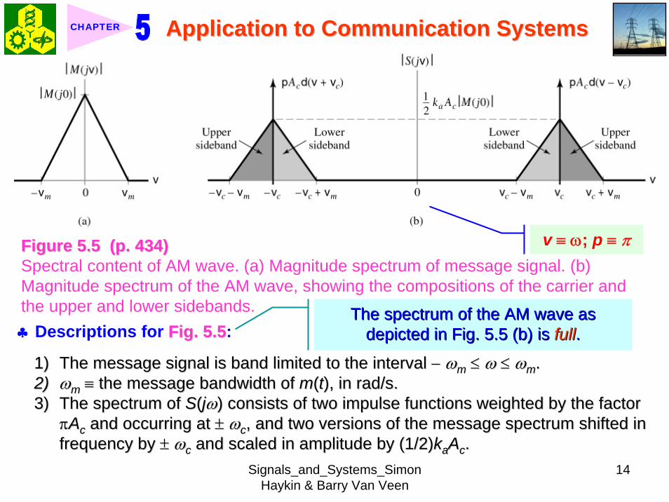
Signals_and_Systems_Simon Haykin amp Barry Van Veen
14
Application to Communication SystemsApplication to Communication SystemsCHAPTER
Figure 55 (p 434)Figure 55 (p 434)Spectral content of AM wave (a) Magnitude spectrum of message signal (b) Magnitude spectrum of the AM wave showing the compositions of the carrier and the upper and lower sidebands
v equiv ω p equiv π
clubs Descriptions for Fig 55Fig 55
1)1) The message signal is band limited to the interval The message signal is band limited to the interval minusminus ωωmm lele ωω lele ωωmm2)2) ωωmm equivequiv the message bandwidth of the message bandwidth of mm((tt) in rads) in rads3)3) The spectrum of The spectrum of SS((jjωω) consists of two impulse functions weighted by the factor ) consists of two impulse functions weighted by the factor
ππAAcc and occurring at and occurring at plusmnplusmn ωωcc and two versions of the message spectrum shifted in and two versions of the message spectrum shifted in frequency by frequency by plusmnplusmn ωωcc and scaled in amplitude by (12)and scaled in amplitude by (12)kkaaAAcc
The spectrum of the AM wave as The spectrum of the AM wave as depicted in Fig 55 (b) is depicted in Fig 55 (b) is fullfull
Signals_and_Systems_Simon Haykin amp Barry Van Veen
15
Application to Communication SystemsApplication to Communication SystemsCHAPTER
4) 4) Upper sideband Upper sideband equivequiv the spectrum lying above the spectrum lying above ωωcc or below or below minusminus ωωcc5) Lower sideband 5) Lower sideband equivequiv the spectrum lying below the spectrum lying below ωωcc or above or above minusminus ωωcc
The condition ωc gt ωm is a necessary condition for the sidebands not to overlap
6) 6) Highest frequency component of the AM wave Highest frequency component of the AM wave equivequiv ωωcc + + ωωmm7) Lowest frequency component of the AM wave 7) Lowest frequency component of the AM wave equivequiv ωωcc minusminus ωωmm8) The difference between these two frequencies defines the tran8) The difference between these two frequencies defines the transmission smission
bandwidth bandwidth ωωTT for an AM wave for an AM wave
2T mω ω= (513)
Example 51 Full Amplitude Modulation for Sinusoidal Modulating SignalConsider a modulating wave m(t) that consists of a single tone or frequency component that is
0 0( ) cos( )m t A tω=
where A0 is the amplitude of the modulating wave and ω0 is its radian frequency (See Fig 56(a)Fig 56(a)) The sinusoidal carrier wave c(t) has amplitude Ac and radian frequency ωc (See Fig 56(b)Fig 56(b)) Evaluate the time-domain and frequency-domain characteristics of the AM wave
Signals_and_Systems_Simon Haykin amp Barry Van Veen
16
Application to Communication SystemsApplication to Communication SystemsCHAPTER
Figure 56 (p Figure 56 (p 435)435)Time-domain (on the left) and frequency-domain (on the right) characteristics of AM produced by a sinusoidal modulating wave (a) Modulating wave (b) Carrier wave (c) AM wave
v equiv ω p equiv π
Signals_and_Systems_Simon Haykin amp Barry Van Veen
17
Application to Communication SystemsApplication to Communication SystemsCHAPTER
ltltSolgtSolgt1 The AM wave is described by
[ ]0( ) 1 cos( ) cos( )c cs t A t tμ ω ω= + (514) where 0ak Aμ =
clubsclubs The dimensionless constant The dimensionless constant μμ for a sinusoidal modulating wave is called the for a sinusoidal modulating wave is called the modulation factormodulation factor and equals the percentage modulation when it is expressedand equals the percentage modulation when it is expressednumerically as a percentage numerically as a percentage
clubsclubs To avoid envelope distortion due to To avoid envelope distortion due to overmodulationovermodulation the modulation factor the modulation factor μμ mustmustbe kept below unitybe kept below unity
clubsclubs Figure 56(c)Figure 56(c) is a sketch of is a sketch of ss((tt) for ) for μμ less than unityless than unity2 Let Amax and Amin denote the maximum and minimum values respectively of
the envelope of the modulated wave Then form Eq(514) we get
max
min
(1 )(1 )
c
c
A AA A
μμ
+=
minusmax min
max min
A AA A
μ minus=
+
3 Expressing the product of the two cosines in Eq (514) as the sum of two sinusoidal waves one having frequency ωc + ω0 and the other havingfrequency ωc-ω0 we get
Signals_and_Systems_Simon Haykin amp Barry Van Veen
18
Application to Communication SystemsApplication to Communication SystemsCHAPTER
102
102
( ) cos( ) cos[( ) ]
cos[( ) ]
c c c c
c c
s t A t A t
A t
ω μ ω ω
μ ω ω
= + +
+ minus
4 Fourier transform of s(t)
10 02
10 02
( ) [ ( ) ( )]
[ ( ) ( )]
[ ( ) ( )]
c c c
c c c
c c c
S j A
A
A
ω π δ ω ω δ ω ω
πμ δ ω ω ω δ ω ω ω
πμ δ ω ω ω δ ω ω ω
= minus + +
+ minus minus + + +
+ minus + + + minus
Thus in ideal terms the spectrum of a full AM wave for the spThus in ideal terms the spectrum of a full AM wave for the special case of ecial case of sinusoidal modulation consists of impulse functions at sinusoidal modulation consists of impulse functions at plusmnplusmn ωωcc ωωcc plusmnplusmn ωω00 and and--ωωc c plusmnplusmn ωω 00 as depicted inas depicted in Fig 56(c)Fig 56(c)
Example 52 Average Power of Sinusoidally Modulated SignalContinuing with Example 51 investigate the effect of varying the modulation factor μ on the power content of the AM wave ltltSolgtSolgt1 In practice the AM wave s(t) is a voltage or current signal
Signals_and_Systems_Simon Haykin amp Barry Van Veen
19
Application to Communication SystemsApplication to Communication SystemsCHAPTER
2 In either case the average power delivered to a 1-ohm load resistor by s(t) is composed of three components whose values are derived from Eq (115) asfollows
1 22
1 2 281 2 28
Carrier power
Upper side- frequency power
Lower side- frequency power
c
c
c
A
A
A
μ
μ
=
=
=
3 The ratio of the total sideband power to the total power in the modulated wave is therefore equal th μ 2(2 + μ 2) which depends only on the modulationfactor μ If μ = 1 (ie if 100 modulation is used) the total power in the twoside frequencies of the resulting AM wave is only one-third of the total powerin the modulated wave
4 Figure 57Figure 57 shows the percentage of total power in both side frequencies and in the carrier plotted against the percentage modulation
Signals_and_Systems_Simon Haykin amp Barry Van Veen
20
Application to Communication SystemsApplication to Communication SystemsCHAPTER
Figure 57 (p 437)Figure 57 (p 437)Variations of carrier power and side-frequency power with percentage modulation of AM wave for the case of sinusoidal modulation
546 546 Spectral OverlapSpectral Overlap1 When ωc lt ωm the modulated signal
s(t) undergoes frequency distortiondue to spectral overlap
Fig 58Fig 58clubs Assume that S(jω) is real valued2 The spectral overlap is produced by two movements
1)1) Movement of the lower sideband into the negative frequency rangeMovement of the lower sideband into the negative frequency range2)2) Movement of the image of the lower sideband into the positive frMovement of the image of the lower sideband into the positive frequency rangeequency range
3 For avoiding the spectral overlap problem the necessary condition is
c mω ωge
Signals_and_Systems_Simon Haykin amp Barry Van Veen
21
Application to Communication SystemsApplication to Communication SystemsCHAPTER
Figure 58 (p 438)Figure 58 (p 438)Spectral overlap phenomenon in amplitude modulation The phenomenon arises when the carrier frequency ωc is less than the highest frequency component ωm of the modulating signal
v equiv ω p equiv π
547 547 Demodulation of AM WaveDemodulation of AM Wave1 The envelope detector provides a simple yet effective device for the
demodulation of a narrowband AM signal for which the percentage modulation is less than 100
clubsclubs Narrowband means that the carrier is large compared with the mesNarrowband means that the carrier is large compared with the message bandwidthsage bandwidth2 Circuit diagram of an envelope detector Fig 59Fig 59
1) 1) The diode is ideal presenting zero impedance to current flow inThe diode is ideal presenting zero impedance to current flow in the forwardthe forward--biased region and infinite impedance in the reversebiased region and infinite impedance in the reverse--biased region biased region
Signals_and_Systems_Simon Haykin amp Barry Van Veen
22
Application to Communication SystemsApplication to Communication SystemsCHAPTER
Figure 59 (p 438)Figure 59 (p 438)Envelope detector illustrated by (a) circuit diagram (b) AM wave input and (c) envelope detector output assuming ideal conditions
Signals_and_Systems_Simon Haykin amp Barry Van Veen
23
Application to Communication SystemsApplication to Communication SystemsCHAPTER
2) 2) The AM signal applied to the envelope is supplied by a voltage sThe AM signal applied to the envelope is supplied by a voltage source of ource of internal resistance internal resistance RRss
3) The load resistance 3) The load resistance RRll is large compared with the source resistance is large compared with the source resistance RRss During Duringthe charging process the time constant is effectively equathe charging process the time constant is effectively equal to l to RRssCC This time This time constant must be short compared with the carrier period 2constant must be short compared with the carrier period 2ππωωcc that is that is
2s
c
R πω
ltlt (515)
3 The discharging time constant is equal to RlCRRllCC must be large such that the capacitor discharges slowly but notmust be large such that the capacitor discharges slowly but not so so large that the capacitor voltage will not discharge at the maximlarge that the capacitor voltage will not discharge at the maximum rate um rate of change of the modulating wave ieof change of the modulating wave ie2 2
lc m
R Cπ πω ω
ltlt ltlt (516) ωm equiv message
bandwidth
clubs Output ripple can be removed by low-pass filter
Signals_and_Systems_Simon Haykin amp Barry Van Veen
24
Application to Communication SystemsApplication to Communication SystemsCHAPTER
55 55 Double SidebandDouble Sideband--Suppressed ModulationSuppressed Modulation1 In full AM carrier wave c(t) is completely independent of the message signal
m(t)
Transmission of carrier wave A waste of power
2 To overcome this shortcoming we may suppress the carrier component from the modulated wave resulting in double sideband-suppressed carrier(DSB-SC) modulation
3 DSB-SC modulated signal( ) ( ) ( ) cos( ) ( )c cs t c t m t A t m tω= = (517)
clubs This modulated signal undergoes a phase reversal whenever the messagesignal m(t) crosses zero as illustrated in Fig 510Fig 510(a)(a) Message signal Message signal (b)(b) DSBDSB--SC modulated wave resulting from multiplication of the message SC modulated wave resulting from multiplication of the message
signal by the sinusoidal carrier wave signal by the sinusoidal carrier wave
Signals_and_Systems_Simon Haykin amp Barry Van Veen
25
Application to Communication SystemsApplication to Communication SystemsCHAPTER
Figure 510 (p 440)Figure 510 (p 440)Double-sideband-suppressed carrier modulation (a) Message signal (b) DSB-SC modulated wave resulting from multiplication of the message signal by the sinusoidal carrier wave
551 551 FrequencyFrequency--Domain DescriptionDomain Description1 Fourier transform of modulated signal s(t)
1( ) [ ( ( )) ( ( ))]2 c c cS j A M j M jω ω ω ω ω= minus + + (518)
where M(jω) equiv Fourier transform of m(t) minus ωm le ω le ωmFig 511 (a) and (b)Fig 511 (a) and (b)
Signals_and_Systems_Simon Haykin amp Barry Van Veen
26
Application to Communication SystemsApplication to Communication SystemsCHAPTER
Figure 511 (p 441)Figure 511 (p 441)Spectral content of DSB-SC modulated wave (a) Magnitude spectrum of message signal (b) Magnitude spectrum of DSB-SC modulated wave consisting of upper and lower sidebands only
v equiv ω p equiv π
clubs The modulation process simply translates the spectrum of the message signal by plusmn ωc
clubs Transmission bandwidth = 2 ωm2 A device for achieving DSB-SC is called a product modulator or simply
multiplierFig 512 (a)Fig 512 (a) shows the block diagram of a product modulator
Signals_and_Systems_Simon Haykin amp Barry Van Veen
27
Application to Communication SystemsApplication to Communication SystemsCHAPTER
Figure 512 (p 441)Figure 512 (p 441)(a) Product modulator for generating the DSB-SC modulated wave (b) Coherent detector for demodulation of the DSB-SC modulated wave
v equiv ω p equiv π
552 552 Coherent DetectionCoherent Detection1 The message signal m(t) may be recovered from DSB-SC
Fig 512 (b)Fig 512 (b)ss((tt) ) timestimes locally generated sinusoidal wave = locally generated sinusoidal wave = vv((tt))vv((tt) filtered by a Low) filtered by a Low--pass filterpass filter
Local oscillator
2 The local oscillator should be exactly coherent or synchronized in both frequency and phase with the carrier wave c(t)
Signals_and_Systems_Simon Haykin amp Barry Van Veen
28
Application to Communication SystemsApplication to Communication SystemsCHAPTER
Coherent detection or synchronization demodulation3 Derivation for coherent detection
1) Local oscillator cos(ωct + φ )2) Product modulator output
( ) cos( ) ( )cos( ) cos( ) ( )
1 1cos( ) ( ) cos(2 ) ( )2 2
c
c c c
c c c
v t t s tA t t m t
A m t A t m t
ω φω ω φ
φ ω φ
= += +
= + +(519)
1 cos( ) ( )2 cA m tφ
1 cos(2 ) ( )2 c cA t m tω φ+
A scaled version of the original message signal m(t)
DSBDSB--SC modulated signal with carrier SC modulated signal with carrier frequency 2 frequency 2 ωωcc
3) Magnitude spectrum Fig 5134) To clear separate two component of v(t) the original carrier frequency ωc
must satisfy the condition
Signals_and_Systems_Simon Haykin amp Barry Van Veen
29
Application to Communication SystemsApplication to Communication SystemsCHAPTER
Figure 513 (p 442)Figure 513 (p 442)Magnitude spectrum of the product modulator output v(t) in the coherent detector of Fig 512(b)
v equiv ω p equiv π
2 c m mω ω ωminus gt c mω ωgt (520) ωωmm equivequiv message bandwidthmessage bandwidth
4 Specification of low-pass filter1) 1) The cutoff frequency must be The cutoff frequency must be ωωm m 2) The transition band must be 2) The transition band must be ωωm m ≦≦ ωω ≦≦ ωωc c ωωm m
Thus the overall output in Thus the overall output in Fig 512(b)Fig 512(b) is given byis given by1( ) cos( ) ( )2o cv t A m tφ= (521)
cosφ equiv attenuation factor
Signals_and_Systems_Simon Haykin amp Barry Van Veen
30
Application to Communication SystemsApplication to Communication SystemsCHAPTER
5 (1) Demodulated signal vo(t) is proportional to m(t) when the error phase φis a constant
(2) Demodulated signal is maximum when φ = 0 and has a minimum zero when φ = plusmn π2
Example 53 Sinusoidal DSB-SC ModulationConsider again the sinusoidal modulating signal
0 0( ) cos( )m t A tω=
( ) cos( )c cc t A tω=with amplitude A0 and frequency ω0 see Fig 514(a) The carrier wave is
with amplitude Ac and frequency ωc see Fig 514(b) Investigate the time-domain and frequency-domain characteristics of the corresponding DSB-SC modulated waveltltSolgtSolgt
clubs φ = plusmn π2 represents the quadrature null effect of the coherent detector
1 The modulated DSB-SC signal is defined by
0 0
0 0 0 0
( ) cos( ) cos( )1 1cos[( ) ] cos[( ) ]2 2
c c
c c c c
s t A A t t
A A t A A t
ω ω
ω ω ω ω
=
= + + minus
Signals_and_Systems_Simon Haykin amp Barry Van Veen
31
Application to Communication SystemsApplication to Communication SystemsCHAPTER
2 The Fourier transform of s(t) is given by
0 0 0
0 0
1( ) cos[ ( ) ( )]2
( ) ( )
c c c
c c
S j A Aω π δ ω ω ω δ ω ω ω
δ ω ω ω δ ω ω ω
= minus minus + + +
+ minus + + + minus
which consists of four weighted impulse functions at the frequencies ωc+ ω0-ωc- ω0 ωc- ω0 and- ωc+ ω0 as illustrated in the right-hand side of Fig Fig 514(c)514(c)
3 This Fourier transform differs from that depicted in the right-hand side of Fig Fig 56(c)56(c) for the corresponding example of full AM in one important respect The impulse functions at plusmn ωc due to the carrier are removed
4 Application of the sinusoidally modulated DSB-SC signal to the product modulator of Fig 512(b) yields the output (assuming φ = 0)
0 0 0
0 0 0 0 0
1( ) cos( ) cos[( ) ] cos[( ) ]21 cos[(2 ) ] cos( ) cos[(2 ) ] cos( )4
c c c c
c c c
v t A A t t t
A A t t t t
ω ω ω ω ω
ω ω ω ω ω ω
= + + minus
= + + + minus +
Signals_and_Systems_Simon Haykin amp Barry Van Veen
32
Application to Communication SystemsApplication to Communication SystemsCHAPTER
Figure 514 (p Figure 514 (p 443)443)Time-domain (on the left) and frequency-domain (on the right) characteristics of DSB-SC modulation produced by a sinusoidal modulating wave (a) Modulating wave (b) Carrier wave (c) DSB-SC modulated wave Note that ω= 2πƒ
v equiv ω p equiv π
Signals_and_Systems_Simon Haykin amp Barry Van Veen
33
Application to Communication SystemsApplication to Communication SystemsCHAPTER
5 The first two sinusoidal terms of v(t) are produced by the upper side frequency and the last two sinusoidal terms are produced by the lower side frequency
6 With ωcgt ω0 the first and third sinusoidal terms of frequencies 2ωc+ ω0 and 2ωc-ω0 respectively are removed by the low-pass filter of Fig 512(b)Fig 512(b) which leaves the second and fourth sinusoidal terms of frequency ω0 as the only output of the filter The coherent detector output thus reproduces the original modulating wave
7 Note however that this output appears as two equal terms one derived from the upper side frequency and the other from the lower side frequency We therefore conclude that for the transmission of the sinusoidal signal A0 cos(ω0t) only one side frequency is necessary (The issue will be discussed further in Section 57Section 57)
553 553 CostasCostas ReceiverReceiver1 Costas receiver Fig 515Fig 5152 This receiver consists of two coherent detector supplied with the same input
ie the incoming DSB-Sc wave
cos(2 ) ( )c cA f t m tπ but with individual local oscillator signals that are in phase duadrature with respect to each other
In-phase coherent detector (I-Channel) and quadrature-phase coherent detector (Q-Channel)
Signals_and_Systems_Simon Haykin amp Barry Van Veen
34
Application to Communication SystemsApplication to Communication SystemsCHAPTER
Figure 515 (p 445)Figure 515 (p 445)Costas receiver
v equiv ω p equiv π
Signals_and_Systems_Simon Haykin amp Barry Van Veen
35
Application to Communication SystemsApplication to Communication SystemsCHAPTER
56 56 QuadratureQuadrature--Carrier MultiplexingCarrier Multiplexing
Figure 516 (p 446)Figure 516 (p 446)Quadrature-carrier multiplexing system exploiting the quadrature null effect (a) Transmitter (b) Receiver assuming perfect synchronization with the transmitter
v equiv ω p equiv π
1 1 A A quadraturequadrature--carrier multiplexing or carrier multiplexing or quadraturequadrature--amplitude modulation (QAM) amplitude modulation (QAM) system enables two DSBsystem enables two DSB--SC modulated waves to occupy the same transmission SC modulated waves to occupy the same transmission bandwidth and yet it allows for their separation at the receivebandwidth and yet it allows for their separation at the receiver outputr output
BandwidthBandwidth--conservation schemeconservation scheme
Signals_and_Systems_Simon Haykin amp Barry Van Veen
36
Application to Communication SystemsApplication to Communication SystemsCHAPTER
2 Fig 5-16(a) Block diagram of the quadrature-carrier multiplexing systemFig 5-16(a) transmitter Fig 5-16(b) receiver
3 Multiplexed signal s(t)
(522) 1 2( ) ( ) cos( ) ( )sin( )c c c cs t A m t t A m t tω ω= +
where m1(t) and m2(t) denotes the two different message signals applied to the product modulations
clubsTransmission bandwidth = 2 ωm centered at ωc where ωm is the commonmessage bandwidth of m1(t) and m2(t)
4 The output of the top detector at receiver is 1
12 ( )cA m t
The output of the bottom detector at receiver is1
22 ( )cA m t
57 57 Other Variants of Amplitude Modulation Other Variants of Amplitude Modulation clubs Basic concept Full AM and DSB-SC rArr Wasteful of bandwidthclubs Given the amplitude and phase spectra of either lower or upper sideband
we can uniquely determine the other
Signals_and_Systems_Simon Haykin amp Barry Van Veen
37
Application to Communication SystemsApplication to Communication SystemsCHAPTER
clubs Single-sideband (SSB) modulation only one sideband is transmitted571 571 FrequencyFrequency--Domain Description of SSB ModulationDomain Description of SSB Modulation1 Consider a message signal m(t) with a spectrum M(jω) limited to the band
ωa le ω le ωb Fig 5-17 (a)2 DSB-SC modulated signal
( ) cos( )c cm t A tωtimes Fig 5-17 (b)
3 (1) Upper sideband the frequencies above ωc and below minus ωc(2) Upper sideband the frequencies below ωc and above minus ωc
Fig 5-17 (c)4 When only the lower sideband is transmitted the spectrum of the
corresponding SSB modulated wave is as shown in Fig 5-17 (d) 5 Advantages of SSB
(1) Reduced bandwidth requirement(2) Elimination of the high-power carrier waveDisadvantage od SSB(1) Cost and complexity of implementing both the transmitter and receiver
Signals_and_Systems_Simon Haykin amp Barry Van Veen
38
Application to Communication SystemsApplication to Communication SystemsCHAPTER
Figure 517 Figure 517 (p 447)(p 447)Frequency-domain characteristics of SSB modulation (a) Magnitude spectrum of message signal with energy gap from ndash ωa to ωa
(c) Magnitude spectrum of SSB modulated wave containing upper sideband only
(d) Magnitude spectrum of SSB modulated wave containing lower sideband only
(b) Magnitude spectrum of DSB-SC signal
v equiv ω p equiv π
Signals_and_Systems_Simon Haykin amp Barry Van Veen
39
Application to Communication SystemsApplication to Communication SystemsCHAPTER
6 Frequency-discrimination scheme for producing SSB modulation Fig 518clubs Bandpass filter is designed to pass the sideband selected for transmission
and suppress the remaining sidebandclubs Requirement in SSB signal the message signal applied to the product
modulator must have a energy gap in its spectrum Refer to Fig 517 (a)
Figure 518 (p 448)Figure 518 (p 448)System consisting of product modulator and bandpass filter for generating SSB modulated wave
v equiv ω p equiv π
572 572 TimeTime--Domain Description of SSB ModulationDomain Description of SSB Modulation1 Mathematical tool Hilbert transform
The Hilbert transform of a signal x(t) is defined by1 ( ) 1ˆ( ) ( )xx t d x t
t tτ τ
π τ πinfin
minusinfin= = lowast
minusint
Signals_and_Systems_Simon Haykin amp Barry Van Veen
40
Application to Communication SystemsApplication to Communication SystemsCHAPTER
The Fourier transform of 1(πt) is minus j times the signum function denoted
1 for 0sgn( ) 0 for 0
1 for 0
ωω ω
ω
+ gt⎧⎪= =⎨⎪minus lt⎩
2 Passing x(t) through a Hilbert transformer is equivalent to the combination of the following two operations in frequency domain1) Keeping X(jω)unchanged for all ω 2) Shifting areX(jω) (ie the phase spectrum of x(t)) by +90deg for negative
frequencies and minus 90deg for positive frequencies clubs Hilbert transformer = Wideband minus 90deg phase shifter 573 573 Vestigial Sideband ModulationVestigial Sideband Modulation1 When the message signal contains significant components at extremely
low frequencies the upper and lower sidebands meet at the carrier frequency
Using SSB is inappropriateUsing SSB is inappropriateEx TV signals or
wideband dataUsing VSB (Vestigial sideband) modulation is appropriateUsing VSB (Vestigial sideband) modulation is appropriate
Signals_and_Systems_Simon Haykin amp Barry Van Veen
41
Application to Communication SystemsApplication to Communication SystemsCHAPTER
2 VSB is a compromise between SSB and DSB-SC forms of modulationIn VSB modulation one sideband is passes almost completely whereas just a trace or vestige of the other sideband is retained
3 Fig 519 illustrates a VSB modulated wave s(t) in relation to the message signal m(t)
v equiv ω p equiv π
Figure 519 (p 449)Figure 519 (p 449)Spectral content of VSB modulated wave (a) Magnitude spectrum of message signal (c) Magnitude spectrum of VSB modulated wave containing a vestige of the lower sideband
clubs The lower sideband is modified into the vestigial sideband4 Transmission bandwidth of VSB modulated wave T m vω ω ω= + (523)
where ωm is the message bandwidth and ωu is the width of the vestigial sideband
Signals_and_Systems_Simon Haykin amp Barry Van Veen
42
Application to Communication SystemsApplication to Communication SystemsCHAPTER
5 Generation of VSB modulated wave Fig 520
Figure 520 (p 450)Figure 520 (p 450)System consisting of product modulator and sideband shaping filter for generating VSB modulated wave
v equiv ω p equiv π
Passing a DSBPassing a DSB--SC modulated wave through a sidebandSC modulated wave through a sideband--shaping filtershaping filter6 The sideband-shaping filter is designed so that the original message
spectrum M(jω) is reproduced on the demodulation as a result of the superposition of two spectra
1) The positive-frequency part of S(jω) (ie the Fourier transform of the transmitted signal s(t)) shifted downward in frequency by ωc
2) The negative-frequency part of S(jω) shifted upward in frequency by ωc
Fig 521 A reflection of the vestige of the lower sideband makes up for the missing parts of the upper sideband
Signals_and_Systems_Simon Haykin amp Barry Van Veen
43
Application to Communication SystemsApplication to Communication SystemsCHAPTER
Figure 521 (p 450)Figure 521 (p 450)Superposition of the two spectra shown in parts (a) and (b) of the figure results in the original message spectrum (shown dashed) upon demodulation
58 58 PulsePulse--Amplitude Modulation Amplitude Modulation clubs Basic concept
Basic role in the operation of AM Frequency-shiftingBasic role in the operation of PAM Sampling
581 581 Sampling RevisitedSampling Revisited1 Sampling theorem
In view point of PAMIn view point of PAM
Signals_and_Systems_Simon Haykin amp Barry Van Veen
44
Application to Communication SystemsApplication to Communication SystemsCHAPTER
1) A band-limited signal of finite energy that has no radian frequency components higher than ωm is uniquely determined by the values of the signal at instants of time separated by π ωm seconds
2) A band-limited signal of finite energy that has no radian frequency components higher than ωm may be completely recovered from a knowledge of its samples taken at the rate of ωm π per seconds
clubs Part 1) rArr Be exploited in the transmitter of a PAM clubs Part 2) rArr Be exploited in the Receiver of a PAM2 To combat the effects of aliasing in practice we use two corrective measures1) Prior to sampling a low-pass antialiasing filter is used to attenuate those high-
frequency components of the signal which lie outside the band of interest2) The filtered signal is sampled at a rate slightly higher than the Nyquist rate3 Generation of a PAM signal Fig 522Fig 522Example 54 Telephonic CommunicationThe highest frequency component of a speech signal needed for telephonic communication is about 31 kHz Suggest a suitable value for the sampling rate ltltSolgtSolgt
Signals_and_Systems_Simon Haykin amp Barry Van Veen
45
Application to Communication SystemsApplication to Communication SystemsCHAPTER
Figure 522 (p 451)Figure 522 (p 451)System consisting of antialiasing filter and sample-and-hold circuit for converting a message signal into a flattopped PAM signal
1 The highest frequency component of 31 kHz corresponds to 362 10 radsmω π= times
Correspondingly the Nyquist rate is
62 kHzmωπ
=
2 A suitable value for the sampling rate-one slightly higher than the Nyquistrate-may be 8 kHz a rate that is the international standard for telephone speech signals
Signals_and_Systems_Simon Haykin amp Barry Van Veen
46
Application to Communication SystemsApplication to Communication SystemsCHAPTER
582 582 Mathematical Description of PAMMathematical Description of PAM1 The carrier wave used in PAM consists of a sequence of short pulses of
fixed duration in terms of which PAM is formally defined as followsPAM is a form of pulse modulation in which the amplitude of the PAM is a form of pulse modulation in which the amplitude of the pulsed carrier is pulsed carrier is varied in accordance with instantaneous sample values of the mesvaried in accordance with instantaneous sample values of the message signalsage signal the duration of the pulsed carrier is maintained constant throughout
Fig 523Fig 523
Figure 523 (p452) Figure 523 (p452) Waveform of flattopped PAM signal with pulse duration T0 and sampling period Ts
Signals_and_Systems_Simon Haykin amp Barry Van Veen
47
Application to Communication SystemsApplication to Communication SystemsCHAPTER
2 Mathematical representation of the PAM
( ) [ ] ( )sn
s t m n b t nTinfin
=minusinfin
= minussum (524) s(t) equiv PAM signal m(t) equiv
message signal
Ts equiv sampling period m[n] equiv the values of m(t) at t = nTs h(t) equiv rectangular pulse of the unit amplitude and duration T0
3 Rectangular pulse
01 0( )
0 otherwiset T
h tlt lt⎧
= ⎨⎩
(525) Fig 524 (a)Fig 524 (a)
clubs Eq (524) is a sample-and-hold operationAnalogous to zeroAnalogous to zero--orderorder--holdhold--
based reconstruction in Sec 46based reconstruction in Sec 46
差異差異hh((tt) ) 的的TTss與與TT00
4 Impulse-sampled version of message signal m(t)
( ) [ ] ( )sn
m t m n t nTδ δinfin
=minusinfin
= minussum (526)
5 PAM signal( ) [ ] ( )
( ) ( )
sn
s t m n b t nT
m t b tδ
infin
=minusinfin
= minus
=
sum(527)
Convolution of impulse-sampled version mδ(t) and h(t)
Time domain Time domain operationoperation
Signals_and_Systems_Simon Haykin amp Barry Van Veen
48
Application to Communication SystemsApplication to Communication SystemsCHAPTER
Figure 524 (p 453)(a) Rectangular pulse h(t) of unit amplitude and duration T0 (b) Magnitude spectrum |H(jω)| and phase spectrum argH(jω) of pulse h(t)
v equiv ω p equiv π
Signals_and_Systems_Simon Haykin amp Barry Van Veen
49
Application to Communication SystemsApplication to Communication SystemsCHAPTER
6 FT of PAM signal( ) ( ) ( )S j M j H jδω ω ω= (528)
where( ) ( )FTS j s tω larr⎯rarr ( ) ( )FTM j m tδ δω larr⎯rarr ( ) ( )FTH j h tω larr⎯rarr
7 Impulse sampling of the message signal m(t) introduces periodicity into the spectrum as given by
1( ) ( ( ))sks
M j M j kTδ ω ω ω
infin
=minusinfin
= minussum (529) 1Ts equiv sampling rate ωs = 2πTs rads
1( ) ( ( )) ( )sks
S j M j k H jT
ω ω ω ωinfin
=minusinfin
= minussum (530)
( ) ( )FTM j m tω larr⎯rarrwhere
clubs Suppose that m(t) is strictly band limited and that the sampling rate 1Ts is greater than the Nyquist rate Then passing s(t) through a reconstruction filter chosen as an ideal low-pass filter with cutoff frequency ωm and gain Ts we find that the spectrum of the resulting filter output is equal to M(jω)H(jω)
Signals_and_Systems_Simon Haykin amp Barry Van Veen
50
Application to Communication SystemsApplication to Communication SystemsCHAPTER
8 From Eq (525) we find that0 2
0 0( ) sin ( (2 )) j TH j T c T e ωω ω π minus= (531) Fig 524(b) magnitude and phase of H(jω)
clubs Using PAM to represent a continuous-time message signal we introduce amplitude distortion as well as a delay of T02
clubs The frequency distortion caused by the use of flat-topped sampled in the generation of a PAM wave illustrated in Fig 523Fig 523 is referred to as the aperture effect
583 583 Demodulation of PAM SignalDemodulation of PAM Signal1 Reconstruction scheme Fig 525Fig 525
Figure 525 (p 454)Figure 525 (p 454)System consisting of low-pass interpolation filter and equalizer for reconstructing a message signal from its flattopped sampled version
clubs The system consists of low-pass interpolation filter and equalizer connected in cascade
Signals_and_Systems_Simon Haykin amp Barry Van Veen
51
Application to Communication SystemsApplication to Communication SystemsCHAPTER
2 The cutoff frequency of low-pass filter = the highest frequency ωm of message signal
3 The equalizer is used to correct the aperture effect due to flat-topped sampling in the sample-and-hold circuit
4 The equalizer has the effect of decreasing the in-band loss of the interpolation filter as frequency increases in such a manner as to compensate for the aperture effect
5 Amplitude response of equalizer
0
0 0 0 0
1 1 1| ( ) | | sinc( 2) | 2 | sin( 2) |
TH j T T T T
ωω ω ω
= =
Frequency response Eq (531)
Example 55 Equalization for PAM TransmissionThe duty cycle in a PAM signal namely T0 Ts is 10 Evaluate the peak amplification required for equalizationltltSolgtSolgt1 At ωm = π Ts which corresponds to the highest frequency component of the
message signal for a sampling rate equal to the Nyquist rate we find from Eq (531) that the magnitude response of the equalizer at ωm normalized to that at zero frequency is
Signals_and_Systems_Simon Haykin amp Barry Van Veen
52
Application to Communication SystemsApplication to Communication SystemsCHAPTER
Figure 526 (p 455)Figure 526 (p 455)Normalized equalization (to compensate for aperture effect) plotted against the duty cycle T0Ts
Signals_and_Systems_Simon Haykin amp Barry Van Veen
53
Application to Communication SystemsApplication to Communication SystemsCHAPTER
0
0 0
( 2)( )1sin (05 ) sin[( 2)( )]
s
s s
T Tc T T T T
ππ
=
where the ratio T0 Ts is equal to the duty cycle of the sampling pulses 2 In Fig 526Fig 526 this result is plotted as a function of the duty cycle T0 Ts Ideally it
should be equal to unity for all values of T0 Ts 3 For a duty cycle of 10 it is equal to 10041 It follows that for duty cycles of less
than 10 the magnitude equalization required is less than 10041 in which case the aperture effect is usually considered to be negligible
59 59 Multiplexing Multiplexing clubs Three basic types of multiplexing1 Frequency-division multiplexing in which the signals are separated by
allocating them to different frequency bands This is illustrated in Fig 527(a) for the case of six different message signals Frequency-division multiplexing favors the use of CW modulation where each message signal is able to use the channel on a continuous-time basis
2 Time-division multiplexing wherein the signals are separated by allocating them to different time slots within a sampling interval
Signals_and_Systems_Simon Haykin amp Barry Van Veen
54
Application to Communication SystemsApplication to Communication SystemsCHAPTER
This second type of multiplexing is illustrated in Fig 527(b) for the case of six different message signals Code-division multiplexing which relies on the assignment of different codes to the individual users of the channel
3 Code-division multiplexing which relies on the assignment of different codes to the individual users of the channel
591 591 FrequencyFrequency--Domain Multiplexing (FDM)Domain Multiplexing (FDM)1 Block diagram Fig 528Fig 5282 Incoming message signals low-pass variety3 Low-pass filter to remove high-frequency components such that the signal
in each channel does not disturb each other4 MOD (modulator) shift the frequency ranges of the signals so as to occupy
mutually exclusive frequency intervalsSSB is often used in this stageEx Voice input is usually assigned a bandwidth of 4 kHz
5 Band-pass filters are used to restrict the band of each modulated wave to its prescribed range
6 Band-pass filters in receiver separate the message signals7 DEM (demodulator) to recover signalsclubs FDM in Fig 528 operates in only one direction
Signals_and_Systems_Simon Haykin amp Barry Van Veen
55
Application to Communication SystemsApplication to Communication SystemsCHAPTER
Figure 527 (p 456)Figure 527 (p 456)Two basic forms of multiplexing (a) Frequency-division multiplexing (with guardbands) (b) Time-division multiplexing no provision is made here for synchronizing pulses
Signals_and_Systems_Simon Haykin amp Barry Van Veen
56
Application to Communication SystemsApplication to Communication SystemsCHAPTER
Figure 528 (p 457)Figure 528 (p 457)Block diagram of FDM system showing the important constituents of the transmitter and receiver
Signals_and_Systems_Simon Haykin amp Barry Van Veen
57
Application to Communication SystemsApplication to Communication SystemsCHAPTER
Example 56 SSB-FDM System
ltltSolgtSolgt
An FDM system is used to multiplex 24 independent voice signals SSB modulation is used for the transmission Given that each voice signal is allotted a bandwidth 4kHz calculate the overall transmission bandwidth of the channel
With each voice signal allotted a bandwidth of 4 kHz the use of SSB modulation requires a bandwidth of 4 kHz for its transmission Accordingly the overall transmission bandwidth provided by the channel is 24 X 4 = 96 kHz 592 592 TimeTime--Domain Multiplexing (TDM)Domain Multiplexing (TDM)clubs Basic to the operation of a TDM system is the sampling theoremclubs The transmission of the message samples engages the transmission channel for
only a fraction of the sampling interval on a periodic basis equal to the width T0 of a PAM modulating pulse
1 Block diagram Fig 529Fig 5292 Commutator is usually implemented by means of electronic switching
circuitry3 The function of commutator is two folds
Signals_and_Systems_Simon Haykin amp Barry Van Veen
58
Application to Communication SystemsApplication to Communication SystemsCHAPTER
Figure 529 (p 458)Figure 529 (p 458)Block diagram of TDM system showing the important constituents of the transmitter and receiver
(1) To take a narrow sample of each of the M input message signals at a rate 1Tsthat is slightly higher than ωcπ where ωc is the cutoff frequency of the input low-pass filter
(2) To sequentially interleave these M samples inside a sampling interval Ts4 Pulse modulator transform the multiplexed signal into a form suitable for
transmission over the common channel
Signals_and_Systems_Simon Haykin amp Barry Van Veen
59
Application to Communication SystemsApplication to Communication SystemsCHAPTER
clubs The use of time-division multiplexing introduces a bandwidth expansion factor M because the scheme must squeeze M samples derived from M independent message sources into a time slot equal to one sampling interval
5 Pulse demodulator performs the inverse operation of the pulse modulator6 Decommutator distributes the narrow samples produced by pulse demodulator to the appropriate low-pass reconstruction filter7 Synchronization between the timing operations of the transmitter and
receiver in a TDM system is essential for satisfactory performance of the system
Inserting an extra pulse into each sampling interval on a regular basisBandwidth expansion factor is increased to M + 1
clubs The TDM system is hghly sensitive to the dispersion in the common transmission channel
Example 57 Comparison of TDM with FDMATDM system is used to multiplex four independent voice signals using PAM Each voice signal is sampled at the rate of 8 kHz The system incorporates a synchronizing pulse train for its proper operation
Signals_and_Systems_Simon Haykin amp Barry Van Veen
60
Application to Communication SystemsApplication to Communication SystemsCHAPTER
(a) Determine the timing relationships between the synchronizing pulse train and the impulse trains used to sample the four voice signals
(b) Calculate the transmission bandwidth of the channel for the TDM system and compare the result with a corresponding FDM system using SSBmodulation
ltltSolgtSolgt(a) The sampling period is
31 125 s
8 10sT s μ= =times
In this example the number of voice signals is M = 4 Hence dividing the sampling period of 125 μs among these voice signals and the synchronizing pulse train we obtain the time slot allocated to each one of them
0 1125 25 s
5
sTTM
μ
=+
= =
Signals_and_Systems_Simon Haykin amp Barry Van Veen
61
Application to Communication SystemsApplication to Communication SystemsCHAPTER
Figure 530Figure 530 shows the timing relationships between the synchronizing pulse train and the four impulse trains used to sample the different voice signals in a single frame Each frame includes time slots of common duration T0 = 25 μs which are allocated to the pulse-modulated signals and synchronizing pulse
Figure 530 (p 459)Figure 530 (p 459)Composition of one frame of a multiplexed PAM signal incorporating four voice-signals and a synchronizing pulse
Signals_and_Systems_Simon Haykin amp Barry Van Veen
62
Application to Communication SystemsApplication to Communication SystemsCHAPTER
(b) As a consequence of the time-bandwidth product (see Section 317) there is an inverse relationship between the duration of a pulse and the bandwidth (ie cutoff frequency) of the channel needed for itstransmission Accordingly the overall transmission bandwidth of the channel is
0
21 1 MHz 40 kHz
25
TTf
T
ωπ
=
= = =
In contrast the use of an FDM system based on SSB modulation requires a channel bandwidth equal to M times that of a single voice signal-that is 4 X 4 = 16 kHz Thus the use of PAM-TDM requires a channel bandwidth that is 40 16 = 25 times that of SSB-FDMIn practice pulse-code modulation is commonly used as the method of modulation for TDM this results in a further increase in channel bandwidth depending on the length of the code word used in the digital representation of each pulse in the PAM signal
Signals_and_Systems_Simon Haykin amp Barry Van Veen
63
Application to Communication SystemsApplication to Communication SystemsCHAPTER
510 510 Pulse and Group Delays Pulse and Group Delays 1 Whenever a signal is transmitted through a dispersive (ie frequency
selective) system some delay is introduced into the output signal in relation to the input signal
2 The delay is determined by the phase response of the system3 Phase response of a dispersive communication channel
( ) arg ( )H jφ ω ω= (532)
A signal is transmitted through the channel at a frequency ωc The signal received at the channel lags the transmitted signal by φ(ωc) The time delay is called phase delay formally defined as
( )cp
c
φ ωτω
= minus (533)
The phase delay is not necessarily the true signal delayclubs Case study for DSB-SC1 Transmitted signal
0( ) cos( ) cos( )cs t A t tω ω= (534)
ωc equiv carrier frequency ω0 equiv sinusoidal modulation frequency
A = AcA0
Signals_and_Systems_Simon Haykin amp Barry Van Veen
64
Application to Communication SystemsApplication to Communication SystemsCHAPTER
1 21 1( ) cos( ) cos( )2 2
s t A t A tω ω= +
1 0cω ω ω= + (535) where
2 0cω ω ω= minus (536)
Upper frequency
Lower frequency
2 Let the s(t) be transmitted through the channel with phase response φ (ω) Accordingly the signal received at the channel output is
1 1 2 21 1( ) cos( ( )) cos( ( ))2 2
y t A t A tω φ ω ω φ ω= + + +
1 2 1 20
( ) ( ) ( )1 ( )( ) cos cos2 2cy t A t tφ ω φ ω φ ω φ ωω ω+⎛ ⎞ ⎛ ⎞= + +⎜ ⎟ ⎜ ⎟
⎝ ⎠ ⎝ ⎠(537)
3 Two observations from Eq (537)1) The carrier component at frequency ωc in y(t) lags its counterpart in s(t) by
frac12 (φ (ω1) + φ (ω2)) which represents a time delay equal to
1 2 1 2
c 1 2
( )+ ( ) ( )+ ( )2 +
φ ω φ ω φ ω φ ωω ω ω
minus = minus (538)
Signals_and_Systems_Simon Haykin amp Barry Van Veen
65
Application to Communication SystemsApplication to Communication SystemsCHAPTER
2) The message component at frequency ω0 in y(t) lags its counterpart in s(t) by frac12 (φ (ω1) minus φ (ω2)) which represents a time delay equal to
1 2 1 2
0 1 2
( ) ( ) ( ) ( )2
φ ω φ ω φ ω φ ωω ω ωminus minus
minus = minusminus
(539)
4 Suppose that ω0 lt ωc rArr the side frequencies are close together with ω c between them Such a modulated signal is said to be a narrowband signal The phase response φ (ω) in the vicinity of ω = ωc is approximated by two-term Taylor series expansion
( )( ) ( ) ( )c
c cd
d ω ω
φ ωφ ω φ ω ω ωω =
= + times minus (540)
Phase delay = ( ) c cφ ω ωminus
5 The time delay introduced by the message signal (ie he ldquoenveloperdquo of the modulated signal) is given by
( )
c
gd
d ω ω
φ ωτω =
= minus (541) The time delay τg is called the
envelope delay or group delay
Signals_and_Systems_Simon Haykin amp Barry Van Veen
66
Application to Communication SystemsApplication to Communication SystemsCHAPTER
6 When a modulated signal is transmitted through a communication channel there are two different delays to be considered1) The carrier or phase delay τp defined by Eq (533)2) The envelope or group delay τg defined by Eq (541)
clubs The group delay is the true signal delay
Example 58 Phase and Group Delays for Ban-pass Channel
ltltSolgtSolgt
The phase response of a band-pass communication channel is defined by 2 2
1( ) tan c
c
ω ωφ ωωω
minus ⎛ ⎞minus= minus ⎜ ⎟
⎝ ⎠The signal s(t) defined in Eq (534) is transmitted through this channel with
475 radscω = 0 025 radsω =andCalculate (a) the phase delay and (b) the group delay
(a) At ω = ωc φ (ωc) = 0 According to Eq (533) the phase delay τ p is zero (b) Differentiating φ (ω) with respect to ω we get
Signals_and_Systems_Simon Haykin amp Barry Van Veen
67
Application to Communication SystemsApplication to Communication SystemsCHAPTER
2 2
2 2 2 2 2
( )( )( )
c c
c c
dd
ω ω ωφ ωω ω ω ω ω
+= minus
+ minus
Using thing result in Eq (541) we find that the group delay is 2 2 04211
475gc
sτω
= = =
1 One waveform shown as a solid curve was obtained by multiplying the transmitted signal s(t) by the carrier wave cos(ωct)
2 The second waveform shown as a dotted curve was obtained by multiplying the received signal y(t) by the carrier wave cos(ωct)
To display the results obtained in parts (a) and (b) in graphical form Fig 531Fig 531shows a superposition of two waveforms obtained as follows
The figure clearly shows that the carrier (phase) delay τ p is zero and the envelope of the received signal y(t) is lagging behind that of the transmitted signal by τs seconds For the presentation of waveforms in this figure we purposely did not use a filter to suppress the high frequency components resulting from the multiplications described under points 1 and 2 because of the desire to retain a contribution due to the carrier for display
Signals_and_Systems_Simon Haykin amp Barry Van Veen
68
Application to Communication SystemsApplication to Communication SystemsCHAPTER
Figure 531 Figure 531 (p 463)(p 463)Highlighting the zero carrier delay (solid curve) and group delay τg (dotted curve) which are determined in accordance with Example 58
Signals_and_Systems_Simon Haykin amp Barry Van Veen
69
Application to Communication SystemsApplication to Communication SystemsCHAPTER
clubs Not also that the separation between the upper side frequency ω1 = ωc + ω0 = 500 rads and the lower side frequency ω2 = ωc minus ω0 = 450 rads is about 10 of the carrier frequency ωc = 475 rads which justifies referring to the modulated signal in this example as a narrowband signal
5101 5101 Some Practical ConsiderationsSome Practical Considerationsclubs What is the practical importance of group delay 1 Eq (541) for determining group delay applies strictly to narrowband
modulated signal2 The message bandwidth may be comparable to the carrier frequency In
this situation the group delay is formulated as a frequency-dependent parameter ie ( )d( )g d
φ ωτ ωω
= minus (542)
3 When a wideband modulated signals transmitted through a dispersive channel the frequency components of the message signal are delayed by different amounts at the channel output
Delay distortionFig 532Fig 532 Group delay response of voice-grade telephone channel
Signals_and_Systems_Simon Haykin amp Barry Van Veen
70
Application to Communication SystemsApplication to Communication SystemsCHAPTER
Figure 532 (p 464)Group delay response of voice-grade telephone channel (Adapted from J C Bellamy Digital Telephony Wiley 1982)
511 511 Exploring Concepts with MATLABExploring Concepts with MATLAB5111 5111 Full AMFull AMclubs Sinusoidal modulation
clubs To reconstruct a faithful version of the original message signal in the receiver we have to use a delay equalizer
0( ) [1 cos( )]cos( )c cs t A t tμ ω ω= +1 AM experiment
1cA =
08 radscω π= 0 01 radsω π=Carrier amplitude
Carrier frequency Modulation amplitude
Signals_and_Systems_Simon Haykin amp Barry Van Veen
71
Application to Communication SystemsApplication to Communication SystemsCHAPTER
2 We wish to display and analyze 10 full cycles of the AM wave corresponding to a total duration of 200 s Choosing a sampling rate 1Ts = 10 Hz we have a total of N = 2000 time samples The frequency band of interest is minus 10 π ≦ ω ≦ 10 π Since the separation between the carrier and either side frequency is equal to the modulation frequency ω0 = 01 π rads we would like to have a frequency resolution ωr = 001π rads To achieve this resolution we require the following number of frequency samples (see Eq (442))
20 2000001
s
r
M ω πω π
ge = =
3 We therefore choose M = 2000 To approximate the Fourier transform of the AM wave s(t) we may use a 2000-point DTFS The only variable in the AM experiment is the modulation factor μ with respect to which we wish to investigate three different situationsμ = 05 corresponding to under-modulationμ = 10 for which the AM system is on the verge of over-modulationμ = 20 corresponding to over-modulation
Signals_and_Systems_Simon Haykin amp Barry Van Veen
72
Application to Communication SystemsApplication to Communication SystemsCHAPTER
4 MATLAB commandsAc = 1 carrier amplitudewc = 08pi carrier frequencyw0 = 01pi modulation frequencymu = 05 modulation factort = 0011999s = Ac(1 + mucos(w0t))cos(wct)plot(ts)Smag = abs(fftshift(fft(s2000)))2000 Smag denotes the magnitude specturm of the AM wavew = 10[-1000999]2pi2000plot(wSmag)axis ([-30 30 0 08])
5 5 μμ = 05 = 05 case case Fig 533Fig 533μμ = 10 case = 10 case Fig 534Fig 534μμ = 20 case = 20 case Fig 535Fig 535
Discussion see pp 466-469 textbook
Signals_and_Systems_Simon Haykin amp Barry Van Veen
73
Application to Communication SystemsApplication to Communication SystemsCHAPTER
-30 -20 -10 0 10 20 300
02
04
06
0 50 100 150 200-2
-1
0
1
2
2 22 24 26 28 3
02
04
06
(a) Time (s)
Time domain
Frequency domain
(b) Frequency (rads)
Frequency domain
Frequency (rads)
Figure 533 (p 466)Amplitude modulation with 50 modulation (a) AM wave (b) magnitude spectrum of the AM wave and (c) expanded spectrum around the carrier frequency
μμ = 05 = 05 casecase
Signals_and_Systems_Simon Haykin amp Barry Van Veen
74
Application to Communication SystemsApplication to Communication SystemsCHAPTER
Figure 534 (p 467)Figure 534 (p 467)Amplitude modulation with 100 modulation (a) AM wave (b) magnitude spectrum of the AM wave and (c) expanded spectrum around the carrier frequency
Signals_and_Systems_Simon Haykin amp Barry Van Veen
75
Application to Communication SystemsApplication to Communication SystemsCHAPTER
Figure 535 (p 468)Amplitude modulation with 200 modulation (a) AM wave (b) magnitude spectrum of the AM wave and (c) expanded spectrum around the carrier frequency
Signals_and_Systems_Simon Haykin amp Barry Van Veen
76
Application to Communication SystemsApplication to Communication SystemsCHAPTER
5112 5112 DSBDSB--SC ModulationSC Modulation1 Sinusoidal modulation
0 0( ) cos( ) cos( )c cs t A A t tω ω=
2 MATLAB commands
Ac = 1 carrier amplitudewc = 08pi carrier frequency in radsA0 = 1 amplitude of modulating signalw0 = 01pi frequency of modulating signalt = 011999s = AcA0cos(wct)cos(w0t)plot(ts)Smag = abs(fftshift(fft(s2000)))2000w = 10[-1000999]2pi2000plot(wSmag)
3 3 DSBDSB--SC modulated waveSC modulated wave Fig 536Fig 536 Discussion see pp 466-469 textbook
4 Output of the product modulator in Fig 512 (b) with φ = 0
Signals_and_Systems_Simon Haykin amp Barry Van Veen
77
Application to Communication SystemsApplication to Communication SystemsCHAPTER
Figure 536 (p 469)DSB-SC modulation (a) DSB-SC modulated wave (b) magnitude spectrum of the modulated wave and (c) expanded spectrum around the carrier frequency
Signals_and_Systems_Simon Haykin amp Barry Van Veen
78
Application to Communication SystemsApplication to Communication SystemsCHAPTER
( ) ( ) cos( )cv t s t tω=
5 MATLAB commandsgtgt v = scos(wct)
6 Fig 537 (a) waveforms of v(t) Fig 537 (b) magnitude spectrum which readily shows that v(t) consists of the following components1) A sinusoidal component with frequency 01π rads representing the
modulating wave2) A new DSB-SC modulated wave with double carrier frequency of 16π rads
in actuality the side frequencies of this modulated wave are located at 15πand 17π rads
1) The frequency of the modulating wave lies inside the passband of the filter2) The upper and lower side frequencies of the new DSB-SC modulated wave
lie inside the stopband of the filter
Accordingly we may recover the sinusoidal modulating signal by passing v(t) through low-pass filter with the following requirements
Signals_and_Systems_Simon Haykin amp Barry Van Veen
79
Application to Communication SystemsApplication to Communication SystemsCHAPTER
Figure 537 (p 470)Coherent detection of DSB-SC modulated wave (a) and (b) Waveform and magnitude spectrum of signal produced at the output of produce modulator (c) and (d) waveform and magnitude spectrum of low-pass filter output
Signals_and_Systems_Simon Haykin amp Barry Van Veen
80
Application to Communication SystemsApplication to Communication SystemsCHAPTER
The issue of how to design a filter with these requirements will be considered in detail in Chapter 8 For the present it suffices to say that the preceding requirements can be met by using the following MATLAB commands
gtgt [ba] = butter(30025)gtgt output = filter(bav)
The first command produces s special type of filter called a Butterworth filter For the experiment considered here the filter order is 3 and its normalized cutoff frequency of 0025 is calculated as follows
Actual cutoff frequency of filter 025 radsHalf the sampling rate 10 rads
0025
ππ
=
=
The second command computes the filterrsquos output in response to the product modulator output v(t) (We will revisit the design of this filter in Chapter 8) Figure 537(c) displays the waveform of the low-pass filter output this waveform represents a sinusoidal signal of frequency 005 Hz an observation that is confirmed by using the ffr command to approximate the spectrum of the filter output The result of the computation is shown in Fig 537(d)Fig 537(d)
Signals_and_Systems_Simon Haykin amp Barry Van Veen
81
Application to Communication SystemsApplication to Communication SystemsCHAPTER
7 In Fig 538 we explore another aspect of DSB-SC modulation namely the effect of varying the modulation frequency Figure 538(a) shows five cycles of a DSB-SC modulated wave that has the same carrier frequency as that in Fig 536(a) but the modulation frequency has been reduced to 0025 Hz( ie a radian frequency of 005π) Figure 538(b) shows the magnitude spectrum of this second DSB-SC modulated wave and its zoomed-in version is shown in Fig 538(c) Comparing this latter figure with Fig 536(c) we see clearly that decreasing the modulation frequency has the effect of moving the upper and lower side frequencies closer together which is consistent with modulation theory
5113 5113 Phase and Group DelayPhase and Group Delay1 In Example 58 we studied the phase and group delays for a band-pass
channel with phase response 2 2
1( ) tan c
c
ω ωφ ωωω
minus ⎛ ⎞minus= minus ⎜ ⎟
⎝ ⎠2 At ω = ωc the phase delay is τ p = 0 and the group delay is τ s = 04211s One
of the wave forms displayed in Fig 531Fig 531 is
1( ) ( ) cos( )cx t s t tω=
Signals_and_Systems_Simon Haykin amp Barry Van Veen
82
Application to Communication SystemsApplication to Communication SystemsCHAPTER
Figure 538 (p 472)Effect of varying the modulation frequency compared with that in Fig 537 (a) and (b) Waveform and magnitude spectrum of DSB-SC modulated wave with a modulation frequency one-half that used in Fig 536 (c) expanded spectrum around the carrier frequency
Signals_and_Systems_Simon Haykin amp Barry Van Veen
83
Application to Communication SystemsApplication to Communication SystemsCHAPTER
where (see page 461)
1 2( ) [cos( ) cos( )]2As t t tω ω= +
and ω1 = ωc + ω0 and ω2 = ωc - ω0 The waveform shown in the figure as a solid curve is a plot of x1(t) The other waveform also displayed in Fig 531Fig 531 is
2
1 1 2 2
( ) ( ) cos( )
[cos( ( )) cos( ( ))]cos( )2
c
c
x t y t tA t t t
ω
ω φ ω ω φ ω ω
=
= + + +
where the angle φ (ω1) and φ (ω2) are the values of the phase response φ (ω) at ω = ω1 and ω = ω2 respectively The waveform shown as a dotted curve in the figure is a plot of x2(t)
3 The generation of x1(t) and x2(t) in MATLAB is achieved with the following commands with A2 set equal to unity
Signals_and_Systems_Simon Haykin amp Barry Van Veen
84
Application to Communication SystemsApplication to Communication SystemsCHAPTER
wc = 475w0 = 025w1 = wc + w0w2 = wc - w0t = -10 0001 10o1 = -atan((w1^2 - wc^2)(w1wc))o2 = -atan((w2^2 - wc^2)(w2wc))s = cos(w1t) + cos(w2t)y = cos(w1t + o1) + cos(w2t + o2)x1 = scos(478t)x2 = ycos(475t)plot(tx1b)hold on plot(tx2k)hold offxlabel(Time)ylabel(Amplitude)
Note that we have set (A2) = 1 for convenience of presentation The function atan in the first two commands returns the arctangent Note also that the computation of both x1 and x2 involve element-by-element multiplications ndash hence the use of period followed by an asterisk
Signals_and_Systems_Simon Haykin amp Barry Van Veen
85
Application to Communication SystemsApplication to Communication SystemsCHAPTER
Signals_and_Systems_Simon Haykin amp Barry Van Veen
86
Application to Communication SystemsApplication to Communication SystemsCHAPTER
Signals_and_Systems_Simon Haykin amp Barry Van Veen
87
Application to Communication SystemsApplication to Communication SystemsCHAPTER
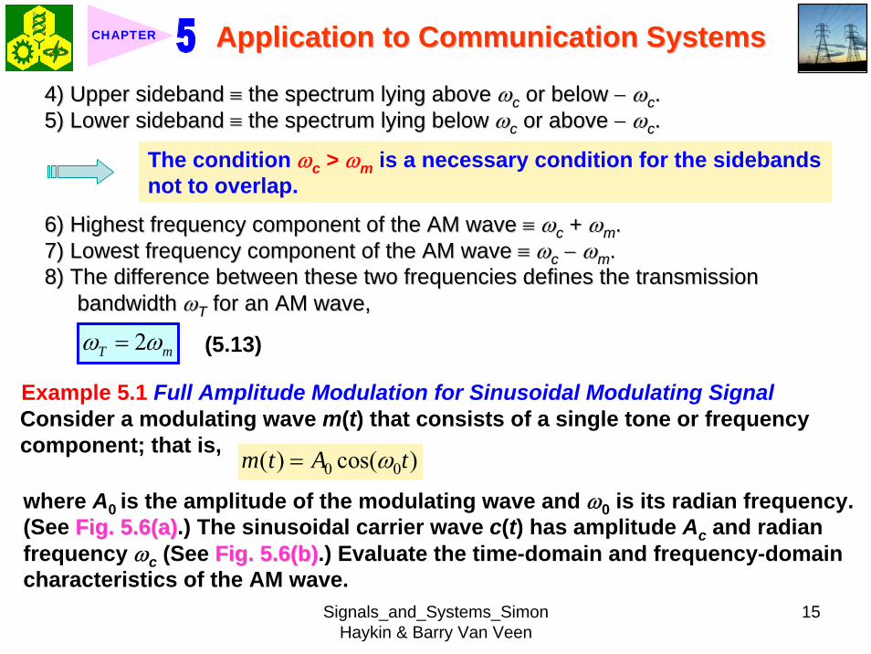
Signals_and_Systems_Simon Haykin amp Barry Van Veen
16
Application to Communication SystemsApplication to Communication SystemsCHAPTER
Figure 56 (p Figure 56 (p 435)435)Time-domain (on the left) and frequency-domain (on the right) characteristics of AM produced by a sinusoidal modulating wave (a) Modulating wave (b) Carrier wave (c) AM wave
v equiv ω p equiv π
Signals_and_Systems_Simon Haykin amp Barry Van Veen
17
Application to Communication SystemsApplication to Communication SystemsCHAPTER
ltltSolgtSolgt1 The AM wave is described by
[ ]0( ) 1 cos( ) cos( )c cs t A t tμ ω ω= + (514) where 0ak Aμ =
clubsclubs The dimensionless constant The dimensionless constant μμ for a sinusoidal modulating wave is called the for a sinusoidal modulating wave is called the modulation factormodulation factor and equals the percentage modulation when it is expressedand equals the percentage modulation when it is expressednumerically as a percentage numerically as a percentage
clubsclubs To avoid envelope distortion due to To avoid envelope distortion due to overmodulationovermodulation the modulation factor the modulation factor μμ mustmustbe kept below unitybe kept below unity
clubsclubs Figure 56(c)Figure 56(c) is a sketch of is a sketch of ss((tt) for ) for μμ less than unityless than unity2 Let Amax and Amin denote the maximum and minimum values respectively of
the envelope of the modulated wave Then form Eq(514) we get
max
min
(1 )(1 )
c
c
A AA A
μμ
+=
minusmax min
max min
A AA A
μ minus=
+
3 Expressing the product of the two cosines in Eq (514) as the sum of two sinusoidal waves one having frequency ωc + ω0 and the other havingfrequency ωc-ω0 we get
Signals_and_Systems_Simon Haykin amp Barry Van Veen
18
Application to Communication SystemsApplication to Communication SystemsCHAPTER
102
102
( ) cos( ) cos[( ) ]
cos[( ) ]
c c c c
c c
s t A t A t
A t
ω μ ω ω
μ ω ω
= + +
+ minus
4 Fourier transform of s(t)
10 02
10 02
( ) [ ( ) ( )]
[ ( ) ( )]
[ ( ) ( )]
c c c
c c c
c c c
S j A
A
A
ω π δ ω ω δ ω ω
πμ δ ω ω ω δ ω ω ω
πμ δ ω ω ω δ ω ω ω
= minus + +
+ minus minus + + +
+ minus + + + minus
Thus in ideal terms the spectrum of a full AM wave for the spThus in ideal terms the spectrum of a full AM wave for the special case of ecial case of sinusoidal modulation consists of impulse functions at sinusoidal modulation consists of impulse functions at plusmnplusmn ωωcc ωωcc plusmnplusmn ωω00 and and--ωωc c plusmnplusmn ωω 00 as depicted inas depicted in Fig 56(c)Fig 56(c)
Example 52 Average Power of Sinusoidally Modulated SignalContinuing with Example 51 investigate the effect of varying the modulation factor μ on the power content of the AM wave ltltSolgtSolgt1 In practice the AM wave s(t) is a voltage or current signal
Signals_and_Systems_Simon Haykin amp Barry Van Veen
19
Application to Communication SystemsApplication to Communication SystemsCHAPTER
2 In either case the average power delivered to a 1-ohm load resistor by s(t) is composed of three components whose values are derived from Eq (115) asfollows
1 22
1 2 281 2 28
Carrier power
Upper side- frequency power
Lower side- frequency power
c
c
c
A
A
A
μ
μ
=
=
=
3 The ratio of the total sideband power to the total power in the modulated wave is therefore equal th μ 2(2 + μ 2) which depends only on the modulationfactor μ If μ = 1 (ie if 100 modulation is used) the total power in the twoside frequencies of the resulting AM wave is only one-third of the total powerin the modulated wave
4 Figure 57Figure 57 shows the percentage of total power in both side frequencies and in the carrier plotted against the percentage modulation
Signals_and_Systems_Simon Haykin amp Barry Van Veen
20
Application to Communication SystemsApplication to Communication SystemsCHAPTER
Figure 57 (p 437)Figure 57 (p 437)Variations of carrier power and side-frequency power with percentage modulation of AM wave for the case of sinusoidal modulation
546 546 Spectral OverlapSpectral Overlap1 When ωc lt ωm the modulated signal
s(t) undergoes frequency distortiondue to spectral overlap
Fig 58Fig 58clubs Assume that S(jω) is real valued2 The spectral overlap is produced by two movements
1)1) Movement of the lower sideband into the negative frequency rangeMovement of the lower sideband into the negative frequency range2)2) Movement of the image of the lower sideband into the positive frMovement of the image of the lower sideband into the positive frequency rangeequency range
3 For avoiding the spectral overlap problem the necessary condition is
c mω ωge
Signals_and_Systems_Simon Haykin amp Barry Van Veen
21
Application to Communication SystemsApplication to Communication SystemsCHAPTER
Figure 58 (p 438)Figure 58 (p 438)Spectral overlap phenomenon in amplitude modulation The phenomenon arises when the carrier frequency ωc is less than the highest frequency component ωm of the modulating signal
v equiv ω p equiv π
547 547 Demodulation of AM WaveDemodulation of AM Wave1 The envelope detector provides a simple yet effective device for the
demodulation of a narrowband AM signal for which the percentage modulation is less than 100
clubsclubs Narrowband means that the carrier is large compared with the mesNarrowband means that the carrier is large compared with the message bandwidthsage bandwidth2 Circuit diagram of an envelope detector Fig 59Fig 59
1) 1) The diode is ideal presenting zero impedance to current flow inThe diode is ideal presenting zero impedance to current flow in the forwardthe forward--biased region and infinite impedance in the reversebiased region and infinite impedance in the reverse--biased region biased region
Signals_and_Systems_Simon Haykin amp Barry Van Veen
22
Application to Communication SystemsApplication to Communication SystemsCHAPTER
Figure 59 (p 438)Figure 59 (p 438)Envelope detector illustrated by (a) circuit diagram (b) AM wave input and (c) envelope detector output assuming ideal conditions
Signals_and_Systems_Simon Haykin amp Barry Van Veen
23
Application to Communication SystemsApplication to Communication SystemsCHAPTER
2) 2) The AM signal applied to the envelope is supplied by a voltage sThe AM signal applied to the envelope is supplied by a voltage source of ource of internal resistance internal resistance RRss
3) The load resistance 3) The load resistance RRll is large compared with the source resistance is large compared with the source resistance RRss During Duringthe charging process the time constant is effectively equathe charging process the time constant is effectively equal to l to RRssCC This time This time constant must be short compared with the carrier period 2constant must be short compared with the carrier period 2ππωωcc that is that is
2s
c
R πω
ltlt (515)
3 The discharging time constant is equal to RlCRRllCC must be large such that the capacitor discharges slowly but notmust be large such that the capacitor discharges slowly but not so so large that the capacitor voltage will not discharge at the maximlarge that the capacitor voltage will not discharge at the maximum rate um rate of change of the modulating wave ieof change of the modulating wave ie2 2
lc m
R Cπ πω ω
ltlt ltlt (516) ωm equiv message
bandwidth
clubs Output ripple can be removed by low-pass filter
Signals_and_Systems_Simon Haykin amp Barry Van Veen
24
Application to Communication SystemsApplication to Communication SystemsCHAPTER
55 55 Double SidebandDouble Sideband--Suppressed ModulationSuppressed Modulation1 In full AM carrier wave c(t) is completely independent of the message signal
m(t)
Transmission of carrier wave A waste of power
2 To overcome this shortcoming we may suppress the carrier component from the modulated wave resulting in double sideband-suppressed carrier(DSB-SC) modulation
3 DSB-SC modulated signal( ) ( ) ( ) cos( ) ( )c cs t c t m t A t m tω= = (517)
clubs This modulated signal undergoes a phase reversal whenever the messagesignal m(t) crosses zero as illustrated in Fig 510Fig 510(a)(a) Message signal Message signal (b)(b) DSBDSB--SC modulated wave resulting from multiplication of the message SC modulated wave resulting from multiplication of the message
signal by the sinusoidal carrier wave signal by the sinusoidal carrier wave
Signals_and_Systems_Simon Haykin amp Barry Van Veen
25
Application to Communication SystemsApplication to Communication SystemsCHAPTER
Figure 510 (p 440)Figure 510 (p 440)Double-sideband-suppressed carrier modulation (a) Message signal (b) DSB-SC modulated wave resulting from multiplication of the message signal by the sinusoidal carrier wave
551 551 FrequencyFrequency--Domain DescriptionDomain Description1 Fourier transform of modulated signal s(t)
1( ) [ ( ( )) ( ( ))]2 c c cS j A M j M jω ω ω ω ω= minus + + (518)
where M(jω) equiv Fourier transform of m(t) minus ωm le ω le ωmFig 511 (a) and (b)Fig 511 (a) and (b)
Signals_and_Systems_Simon Haykin amp Barry Van Veen
26
Application to Communication SystemsApplication to Communication SystemsCHAPTER
Figure 511 (p 441)Figure 511 (p 441)Spectral content of DSB-SC modulated wave (a) Magnitude spectrum of message signal (b) Magnitude spectrum of DSB-SC modulated wave consisting of upper and lower sidebands only
v equiv ω p equiv π
clubs The modulation process simply translates the spectrum of the message signal by plusmn ωc
clubs Transmission bandwidth = 2 ωm2 A device for achieving DSB-SC is called a product modulator or simply
multiplierFig 512 (a)Fig 512 (a) shows the block diagram of a product modulator
Signals_and_Systems_Simon Haykin amp Barry Van Veen
27
Application to Communication SystemsApplication to Communication SystemsCHAPTER
Figure 512 (p 441)Figure 512 (p 441)(a) Product modulator for generating the DSB-SC modulated wave (b) Coherent detector for demodulation of the DSB-SC modulated wave
v equiv ω p equiv π
552 552 Coherent DetectionCoherent Detection1 The message signal m(t) may be recovered from DSB-SC
Fig 512 (b)Fig 512 (b)ss((tt) ) timestimes locally generated sinusoidal wave = locally generated sinusoidal wave = vv((tt))vv((tt) filtered by a Low) filtered by a Low--pass filterpass filter
Local oscillator
2 The local oscillator should be exactly coherent or synchronized in both frequency and phase with the carrier wave c(t)
Signals_and_Systems_Simon Haykin amp Barry Van Veen
28
Application to Communication SystemsApplication to Communication SystemsCHAPTER
Coherent detection or synchronization demodulation3 Derivation for coherent detection
1) Local oscillator cos(ωct + φ )2) Product modulator output
( ) cos( ) ( )cos( ) cos( ) ( )
1 1cos( ) ( ) cos(2 ) ( )2 2
c
c c c
c c c
v t t s tA t t m t
A m t A t m t
ω φω ω φ
φ ω φ
= += +
= + +(519)
1 cos( ) ( )2 cA m tφ
1 cos(2 ) ( )2 c cA t m tω φ+
A scaled version of the original message signal m(t)
DSBDSB--SC modulated signal with carrier SC modulated signal with carrier frequency 2 frequency 2 ωωcc
3) Magnitude spectrum Fig 5134) To clear separate two component of v(t) the original carrier frequency ωc
must satisfy the condition
Signals_and_Systems_Simon Haykin amp Barry Van Veen
29
Application to Communication SystemsApplication to Communication SystemsCHAPTER
Figure 513 (p 442)Figure 513 (p 442)Magnitude spectrum of the product modulator output v(t) in the coherent detector of Fig 512(b)
v equiv ω p equiv π
2 c m mω ω ωminus gt c mω ωgt (520) ωωmm equivequiv message bandwidthmessage bandwidth
4 Specification of low-pass filter1) 1) The cutoff frequency must be The cutoff frequency must be ωωm m 2) The transition band must be 2) The transition band must be ωωm m ≦≦ ωω ≦≦ ωωc c ωωm m
Thus the overall output in Thus the overall output in Fig 512(b)Fig 512(b) is given byis given by1( ) cos( ) ( )2o cv t A m tφ= (521)
cosφ equiv attenuation factor
Signals_and_Systems_Simon Haykin amp Barry Van Veen
30
Application to Communication SystemsApplication to Communication SystemsCHAPTER
5 (1) Demodulated signal vo(t) is proportional to m(t) when the error phase φis a constant
(2) Demodulated signal is maximum when φ = 0 and has a minimum zero when φ = plusmn π2
Example 53 Sinusoidal DSB-SC ModulationConsider again the sinusoidal modulating signal
0 0( ) cos( )m t A tω=
( ) cos( )c cc t A tω=with amplitude A0 and frequency ω0 see Fig 514(a) The carrier wave is
with amplitude Ac and frequency ωc see Fig 514(b) Investigate the time-domain and frequency-domain characteristics of the corresponding DSB-SC modulated waveltltSolgtSolgt
clubs φ = plusmn π2 represents the quadrature null effect of the coherent detector
1 The modulated DSB-SC signal is defined by
0 0
0 0 0 0
( ) cos( ) cos( )1 1cos[( ) ] cos[( ) ]2 2
c c
c c c c
s t A A t t
A A t A A t
ω ω
ω ω ω ω
=
= + + minus
Signals_and_Systems_Simon Haykin amp Barry Van Veen
31
Application to Communication SystemsApplication to Communication SystemsCHAPTER
2 The Fourier transform of s(t) is given by
0 0 0
0 0
1( ) cos[ ( ) ( )]2
( ) ( )
c c c
c c
S j A Aω π δ ω ω ω δ ω ω ω
δ ω ω ω δ ω ω ω
= minus minus + + +
+ minus + + + minus
which consists of four weighted impulse functions at the frequencies ωc+ ω0-ωc- ω0 ωc- ω0 and- ωc+ ω0 as illustrated in the right-hand side of Fig Fig 514(c)514(c)
3 This Fourier transform differs from that depicted in the right-hand side of Fig Fig 56(c)56(c) for the corresponding example of full AM in one important respect The impulse functions at plusmn ωc due to the carrier are removed
4 Application of the sinusoidally modulated DSB-SC signal to the product modulator of Fig 512(b) yields the output (assuming φ = 0)
0 0 0
0 0 0 0 0
1( ) cos( ) cos[( ) ] cos[( ) ]21 cos[(2 ) ] cos( ) cos[(2 ) ] cos( )4
c c c c
c c c
v t A A t t t
A A t t t t
ω ω ω ω ω
ω ω ω ω ω ω
= + + minus
= + + + minus +
Signals_and_Systems_Simon Haykin amp Barry Van Veen
32
Application to Communication SystemsApplication to Communication SystemsCHAPTER
Figure 514 (p Figure 514 (p 443)443)Time-domain (on the left) and frequency-domain (on the right) characteristics of DSB-SC modulation produced by a sinusoidal modulating wave (a) Modulating wave (b) Carrier wave (c) DSB-SC modulated wave Note that ω= 2πƒ
v equiv ω p equiv π
Signals_and_Systems_Simon Haykin amp Barry Van Veen
33
Application to Communication SystemsApplication to Communication SystemsCHAPTER
5 The first two sinusoidal terms of v(t) are produced by the upper side frequency and the last two sinusoidal terms are produced by the lower side frequency
6 With ωcgt ω0 the first and third sinusoidal terms of frequencies 2ωc+ ω0 and 2ωc-ω0 respectively are removed by the low-pass filter of Fig 512(b)Fig 512(b) which leaves the second and fourth sinusoidal terms of frequency ω0 as the only output of the filter The coherent detector output thus reproduces the original modulating wave
7 Note however that this output appears as two equal terms one derived from the upper side frequency and the other from the lower side frequency We therefore conclude that for the transmission of the sinusoidal signal A0 cos(ω0t) only one side frequency is necessary (The issue will be discussed further in Section 57Section 57)
553 553 CostasCostas ReceiverReceiver1 Costas receiver Fig 515Fig 5152 This receiver consists of two coherent detector supplied with the same input
ie the incoming DSB-Sc wave
cos(2 ) ( )c cA f t m tπ but with individual local oscillator signals that are in phase duadrature with respect to each other
In-phase coherent detector (I-Channel) and quadrature-phase coherent detector (Q-Channel)
Signals_and_Systems_Simon Haykin amp Barry Van Veen
34
Application to Communication SystemsApplication to Communication SystemsCHAPTER
Figure 515 (p 445)Figure 515 (p 445)Costas receiver
v equiv ω p equiv π
Signals_and_Systems_Simon Haykin amp Barry Van Veen
35
Application to Communication SystemsApplication to Communication SystemsCHAPTER
56 56 QuadratureQuadrature--Carrier MultiplexingCarrier Multiplexing
Figure 516 (p 446)Figure 516 (p 446)Quadrature-carrier multiplexing system exploiting the quadrature null effect (a) Transmitter (b) Receiver assuming perfect synchronization with the transmitter
v equiv ω p equiv π
1 1 A A quadraturequadrature--carrier multiplexing or carrier multiplexing or quadraturequadrature--amplitude modulation (QAM) amplitude modulation (QAM) system enables two DSBsystem enables two DSB--SC modulated waves to occupy the same transmission SC modulated waves to occupy the same transmission bandwidth and yet it allows for their separation at the receivebandwidth and yet it allows for their separation at the receiver outputr output
BandwidthBandwidth--conservation schemeconservation scheme
Signals_and_Systems_Simon Haykin amp Barry Van Veen
36
Application to Communication SystemsApplication to Communication SystemsCHAPTER
2 Fig 5-16(a) Block diagram of the quadrature-carrier multiplexing systemFig 5-16(a) transmitter Fig 5-16(b) receiver
3 Multiplexed signal s(t)
(522) 1 2( ) ( ) cos( ) ( )sin( )c c c cs t A m t t A m t tω ω= +
where m1(t) and m2(t) denotes the two different message signals applied to the product modulations
clubsTransmission bandwidth = 2 ωm centered at ωc where ωm is the commonmessage bandwidth of m1(t) and m2(t)
4 The output of the top detector at receiver is 1
12 ( )cA m t
The output of the bottom detector at receiver is1
22 ( )cA m t
57 57 Other Variants of Amplitude Modulation Other Variants of Amplitude Modulation clubs Basic concept Full AM and DSB-SC rArr Wasteful of bandwidthclubs Given the amplitude and phase spectra of either lower or upper sideband
we can uniquely determine the other
Signals_and_Systems_Simon Haykin amp Barry Van Veen
37
Application to Communication SystemsApplication to Communication SystemsCHAPTER
clubs Single-sideband (SSB) modulation only one sideband is transmitted571 571 FrequencyFrequency--Domain Description of SSB ModulationDomain Description of SSB Modulation1 Consider a message signal m(t) with a spectrum M(jω) limited to the band
ωa le ω le ωb Fig 5-17 (a)2 DSB-SC modulated signal
( ) cos( )c cm t A tωtimes Fig 5-17 (b)
3 (1) Upper sideband the frequencies above ωc and below minus ωc(2) Upper sideband the frequencies below ωc and above minus ωc
Fig 5-17 (c)4 When only the lower sideband is transmitted the spectrum of the
corresponding SSB modulated wave is as shown in Fig 5-17 (d) 5 Advantages of SSB
(1) Reduced bandwidth requirement(2) Elimination of the high-power carrier waveDisadvantage od SSB(1) Cost and complexity of implementing both the transmitter and receiver
Signals_and_Systems_Simon Haykin amp Barry Van Veen
38
Application to Communication SystemsApplication to Communication SystemsCHAPTER
Figure 517 Figure 517 (p 447)(p 447)Frequency-domain characteristics of SSB modulation (a) Magnitude spectrum of message signal with energy gap from ndash ωa to ωa
(c) Magnitude spectrum of SSB modulated wave containing upper sideband only
(d) Magnitude spectrum of SSB modulated wave containing lower sideband only
(b) Magnitude spectrum of DSB-SC signal
v equiv ω p equiv π
Signals_and_Systems_Simon Haykin amp Barry Van Veen
39
Application to Communication SystemsApplication to Communication SystemsCHAPTER
6 Frequency-discrimination scheme for producing SSB modulation Fig 518clubs Bandpass filter is designed to pass the sideband selected for transmission
and suppress the remaining sidebandclubs Requirement in SSB signal the message signal applied to the product
modulator must have a energy gap in its spectrum Refer to Fig 517 (a)
Figure 518 (p 448)Figure 518 (p 448)System consisting of product modulator and bandpass filter for generating SSB modulated wave
v equiv ω p equiv π
572 572 TimeTime--Domain Description of SSB ModulationDomain Description of SSB Modulation1 Mathematical tool Hilbert transform
The Hilbert transform of a signal x(t) is defined by1 ( ) 1ˆ( ) ( )xx t d x t
t tτ τ
π τ πinfin
minusinfin= = lowast
minusint
Signals_and_Systems_Simon Haykin amp Barry Van Veen
40
Application to Communication SystemsApplication to Communication SystemsCHAPTER
The Fourier transform of 1(πt) is minus j times the signum function denoted
1 for 0sgn( ) 0 for 0
1 for 0
ωω ω
ω
+ gt⎧⎪= =⎨⎪minus lt⎩
2 Passing x(t) through a Hilbert transformer is equivalent to the combination of the following two operations in frequency domain1) Keeping X(jω)unchanged for all ω 2) Shifting areX(jω) (ie the phase spectrum of x(t)) by +90deg for negative
frequencies and minus 90deg for positive frequencies clubs Hilbert transformer = Wideband minus 90deg phase shifter 573 573 Vestigial Sideband ModulationVestigial Sideband Modulation1 When the message signal contains significant components at extremely
low frequencies the upper and lower sidebands meet at the carrier frequency
Using SSB is inappropriateUsing SSB is inappropriateEx TV signals or
wideband dataUsing VSB (Vestigial sideband) modulation is appropriateUsing VSB (Vestigial sideband) modulation is appropriate
Signals_and_Systems_Simon Haykin amp Barry Van Veen
41
Application to Communication SystemsApplication to Communication SystemsCHAPTER
2 VSB is a compromise between SSB and DSB-SC forms of modulationIn VSB modulation one sideband is passes almost completely whereas just a trace or vestige of the other sideband is retained
3 Fig 519 illustrates a VSB modulated wave s(t) in relation to the message signal m(t)
v equiv ω p equiv π
Figure 519 (p 449)Figure 519 (p 449)Spectral content of VSB modulated wave (a) Magnitude spectrum of message signal (c) Magnitude spectrum of VSB modulated wave containing a vestige of the lower sideband
clubs The lower sideband is modified into the vestigial sideband4 Transmission bandwidth of VSB modulated wave T m vω ω ω= + (523)
where ωm is the message bandwidth and ωu is the width of the vestigial sideband
Signals_and_Systems_Simon Haykin amp Barry Van Veen
42
Application to Communication SystemsApplication to Communication SystemsCHAPTER
5 Generation of VSB modulated wave Fig 520
Figure 520 (p 450)Figure 520 (p 450)System consisting of product modulator and sideband shaping filter for generating VSB modulated wave
v equiv ω p equiv π
Passing a DSBPassing a DSB--SC modulated wave through a sidebandSC modulated wave through a sideband--shaping filtershaping filter6 The sideband-shaping filter is designed so that the original message
spectrum M(jω) is reproduced on the demodulation as a result of the superposition of two spectra
1) The positive-frequency part of S(jω) (ie the Fourier transform of the transmitted signal s(t)) shifted downward in frequency by ωc
2) The negative-frequency part of S(jω) shifted upward in frequency by ωc
Fig 521 A reflection of the vestige of the lower sideband makes up for the missing parts of the upper sideband
Signals_and_Systems_Simon Haykin amp Barry Van Veen
43
Application to Communication SystemsApplication to Communication SystemsCHAPTER
Figure 521 (p 450)Figure 521 (p 450)Superposition of the two spectra shown in parts (a) and (b) of the figure results in the original message spectrum (shown dashed) upon demodulation
58 58 PulsePulse--Amplitude Modulation Amplitude Modulation clubs Basic concept
Basic role in the operation of AM Frequency-shiftingBasic role in the operation of PAM Sampling
581 581 Sampling RevisitedSampling Revisited1 Sampling theorem
In view point of PAMIn view point of PAM
Signals_and_Systems_Simon Haykin amp Barry Van Veen
44
Application to Communication SystemsApplication to Communication SystemsCHAPTER
1) A band-limited signal of finite energy that has no radian frequency components higher than ωm is uniquely determined by the values of the signal at instants of time separated by π ωm seconds
2) A band-limited signal of finite energy that has no radian frequency components higher than ωm may be completely recovered from a knowledge of its samples taken at the rate of ωm π per seconds
clubs Part 1) rArr Be exploited in the transmitter of a PAM clubs Part 2) rArr Be exploited in the Receiver of a PAM2 To combat the effects of aliasing in practice we use two corrective measures1) Prior to sampling a low-pass antialiasing filter is used to attenuate those high-
frequency components of the signal which lie outside the band of interest2) The filtered signal is sampled at a rate slightly higher than the Nyquist rate3 Generation of a PAM signal Fig 522Fig 522Example 54 Telephonic CommunicationThe highest frequency component of a speech signal needed for telephonic communication is about 31 kHz Suggest a suitable value for the sampling rate ltltSolgtSolgt
Signals_and_Systems_Simon Haykin amp Barry Van Veen
45
Application to Communication SystemsApplication to Communication SystemsCHAPTER
Figure 522 (p 451)Figure 522 (p 451)System consisting of antialiasing filter and sample-and-hold circuit for converting a message signal into a flattopped PAM signal
1 The highest frequency component of 31 kHz corresponds to 362 10 radsmω π= times
Correspondingly the Nyquist rate is
62 kHzmωπ
=
2 A suitable value for the sampling rate-one slightly higher than the Nyquistrate-may be 8 kHz a rate that is the international standard for telephone speech signals
Signals_and_Systems_Simon Haykin amp Barry Van Veen
46
Application to Communication SystemsApplication to Communication SystemsCHAPTER
582 582 Mathematical Description of PAMMathematical Description of PAM1 The carrier wave used in PAM consists of a sequence of short pulses of
fixed duration in terms of which PAM is formally defined as followsPAM is a form of pulse modulation in which the amplitude of the PAM is a form of pulse modulation in which the amplitude of the pulsed carrier is pulsed carrier is varied in accordance with instantaneous sample values of the mesvaried in accordance with instantaneous sample values of the message signalsage signal the duration of the pulsed carrier is maintained constant throughout
Fig 523Fig 523
Figure 523 (p452) Figure 523 (p452) Waveform of flattopped PAM signal with pulse duration T0 and sampling period Ts
Signals_and_Systems_Simon Haykin amp Barry Van Veen
47
Application to Communication SystemsApplication to Communication SystemsCHAPTER
2 Mathematical representation of the PAM
( ) [ ] ( )sn
s t m n b t nTinfin
=minusinfin
= minussum (524) s(t) equiv PAM signal m(t) equiv
message signal
Ts equiv sampling period m[n] equiv the values of m(t) at t = nTs h(t) equiv rectangular pulse of the unit amplitude and duration T0
3 Rectangular pulse
01 0( )
0 otherwiset T
h tlt lt⎧
= ⎨⎩
(525) Fig 524 (a)Fig 524 (a)
clubs Eq (524) is a sample-and-hold operationAnalogous to zeroAnalogous to zero--orderorder--holdhold--
based reconstruction in Sec 46based reconstruction in Sec 46
差異差異hh((tt) ) 的的TTss與與TT00
4 Impulse-sampled version of message signal m(t)
( ) [ ] ( )sn
m t m n t nTδ δinfin
=minusinfin
= minussum (526)
5 PAM signal( ) [ ] ( )
( ) ( )
sn
s t m n b t nT
m t b tδ
infin
=minusinfin
= minus
=
sum(527)
Convolution of impulse-sampled version mδ(t) and h(t)
Time domain Time domain operationoperation
Signals_and_Systems_Simon Haykin amp Barry Van Veen
48
Application to Communication SystemsApplication to Communication SystemsCHAPTER
Figure 524 (p 453)(a) Rectangular pulse h(t) of unit amplitude and duration T0 (b) Magnitude spectrum |H(jω)| and phase spectrum argH(jω) of pulse h(t)
v equiv ω p equiv π
Signals_and_Systems_Simon Haykin amp Barry Van Veen
49
Application to Communication SystemsApplication to Communication SystemsCHAPTER
6 FT of PAM signal( ) ( ) ( )S j M j H jδω ω ω= (528)
where( ) ( )FTS j s tω larr⎯rarr ( ) ( )FTM j m tδ δω larr⎯rarr ( ) ( )FTH j h tω larr⎯rarr
7 Impulse sampling of the message signal m(t) introduces periodicity into the spectrum as given by
1( ) ( ( ))sks
M j M j kTδ ω ω ω
infin
=minusinfin
= minussum (529) 1Ts equiv sampling rate ωs = 2πTs rads
1( ) ( ( )) ( )sks
S j M j k H jT
ω ω ω ωinfin
=minusinfin
= minussum (530)
( ) ( )FTM j m tω larr⎯rarrwhere
clubs Suppose that m(t) is strictly band limited and that the sampling rate 1Ts is greater than the Nyquist rate Then passing s(t) through a reconstruction filter chosen as an ideal low-pass filter with cutoff frequency ωm and gain Ts we find that the spectrum of the resulting filter output is equal to M(jω)H(jω)
Signals_and_Systems_Simon Haykin amp Barry Van Veen
50
Application to Communication SystemsApplication to Communication SystemsCHAPTER
8 From Eq (525) we find that0 2
0 0( ) sin ( (2 )) j TH j T c T e ωω ω π minus= (531) Fig 524(b) magnitude and phase of H(jω)
clubs Using PAM to represent a continuous-time message signal we introduce amplitude distortion as well as a delay of T02
clubs The frequency distortion caused by the use of flat-topped sampled in the generation of a PAM wave illustrated in Fig 523Fig 523 is referred to as the aperture effect
583 583 Demodulation of PAM SignalDemodulation of PAM Signal1 Reconstruction scheme Fig 525Fig 525
Figure 525 (p 454)Figure 525 (p 454)System consisting of low-pass interpolation filter and equalizer for reconstructing a message signal from its flattopped sampled version
clubs The system consists of low-pass interpolation filter and equalizer connected in cascade
Signals_and_Systems_Simon Haykin amp Barry Van Veen
51
Application to Communication SystemsApplication to Communication SystemsCHAPTER
2 The cutoff frequency of low-pass filter = the highest frequency ωm of message signal
3 The equalizer is used to correct the aperture effect due to flat-topped sampling in the sample-and-hold circuit
4 The equalizer has the effect of decreasing the in-band loss of the interpolation filter as frequency increases in such a manner as to compensate for the aperture effect
5 Amplitude response of equalizer
0
0 0 0 0
1 1 1| ( ) | | sinc( 2) | 2 | sin( 2) |
TH j T T T T
ωω ω ω
= =
Frequency response Eq (531)
Example 55 Equalization for PAM TransmissionThe duty cycle in a PAM signal namely T0 Ts is 10 Evaluate the peak amplification required for equalizationltltSolgtSolgt1 At ωm = π Ts which corresponds to the highest frequency component of the
message signal for a sampling rate equal to the Nyquist rate we find from Eq (531) that the magnitude response of the equalizer at ωm normalized to that at zero frequency is
Signals_and_Systems_Simon Haykin amp Barry Van Veen
52
Application to Communication SystemsApplication to Communication SystemsCHAPTER
Figure 526 (p 455)Figure 526 (p 455)Normalized equalization (to compensate for aperture effect) plotted against the duty cycle T0Ts
Signals_and_Systems_Simon Haykin amp Barry Van Veen
53
Application to Communication SystemsApplication to Communication SystemsCHAPTER
0
0 0
( 2)( )1sin (05 ) sin[( 2)( )]
s
s s
T Tc T T T T
ππ
=
where the ratio T0 Ts is equal to the duty cycle of the sampling pulses 2 In Fig 526Fig 526 this result is plotted as a function of the duty cycle T0 Ts Ideally it
should be equal to unity for all values of T0 Ts 3 For a duty cycle of 10 it is equal to 10041 It follows that for duty cycles of less
than 10 the magnitude equalization required is less than 10041 in which case the aperture effect is usually considered to be negligible
59 59 Multiplexing Multiplexing clubs Three basic types of multiplexing1 Frequency-division multiplexing in which the signals are separated by
allocating them to different frequency bands This is illustrated in Fig 527(a) for the case of six different message signals Frequency-division multiplexing favors the use of CW modulation where each message signal is able to use the channel on a continuous-time basis
2 Time-division multiplexing wherein the signals are separated by allocating them to different time slots within a sampling interval
Signals_and_Systems_Simon Haykin amp Barry Van Veen
54
Application to Communication SystemsApplication to Communication SystemsCHAPTER
This second type of multiplexing is illustrated in Fig 527(b) for the case of six different message signals Code-division multiplexing which relies on the assignment of different codes to the individual users of the channel
3 Code-division multiplexing which relies on the assignment of different codes to the individual users of the channel
591 591 FrequencyFrequency--Domain Multiplexing (FDM)Domain Multiplexing (FDM)1 Block diagram Fig 528Fig 5282 Incoming message signals low-pass variety3 Low-pass filter to remove high-frequency components such that the signal
in each channel does not disturb each other4 MOD (modulator) shift the frequency ranges of the signals so as to occupy
mutually exclusive frequency intervalsSSB is often used in this stageEx Voice input is usually assigned a bandwidth of 4 kHz
5 Band-pass filters are used to restrict the band of each modulated wave to its prescribed range
6 Band-pass filters in receiver separate the message signals7 DEM (demodulator) to recover signalsclubs FDM in Fig 528 operates in only one direction
Signals_and_Systems_Simon Haykin amp Barry Van Veen
55
Application to Communication SystemsApplication to Communication SystemsCHAPTER
Figure 527 (p 456)Figure 527 (p 456)Two basic forms of multiplexing (a) Frequency-division multiplexing (with guardbands) (b) Time-division multiplexing no provision is made here for synchronizing pulses
Signals_and_Systems_Simon Haykin amp Barry Van Veen
56
Application to Communication SystemsApplication to Communication SystemsCHAPTER
Figure 528 (p 457)Figure 528 (p 457)Block diagram of FDM system showing the important constituents of the transmitter and receiver
Signals_and_Systems_Simon Haykin amp Barry Van Veen
57
Application to Communication SystemsApplication to Communication SystemsCHAPTER
Example 56 SSB-FDM System
ltltSolgtSolgt
An FDM system is used to multiplex 24 independent voice signals SSB modulation is used for the transmission Given that each voice signal is allotted a bandwidth 4kHz calculate the overall transmission bandwidth of the channel
With each voice signal allotted a bandwidth of 4 kHz the use of SSB modulation requires a bandwidth of 4 kHz for its transmission Accordingly the overall transmission bandwidth provided by the channel is 24 X 4 = 96 kHz 592 592 TimeTime--Domain Multiplexing (TDM)Domain Multiplexing (TDM)clubs Basic to the operation of a TDM system is the sampling theoremclubs The transmission of the message samples engages the transmission channel for
only a fraction of the sampling interval on a periodic basis equal to the width T0 of a PAM modulating pulse
1 Block diagram Fig 529Fig 5292 Commutator is usually implemented by means of electronic switching
circuitry3 The function of commutator is two folds
Signals_and_Systems_Simon Haykin amp Barry Van Veen
58
Application to Communication SystemsApplication to Communication SystemsCHAPTER
Figure 529 (p 458)Figure 529 (p 458)Block diagram of TDM system showing the important constituents of the transmitter and receiver
(1) To take a narrow sample of each of the M input message signals at a rate 1Tsthat is slightly higher than ωcπ where ωc is the cutoff frequency of the input low-pass filter
(2) To sequentially interleave these M samples inside a sampling interval Ts4 Pulse modulator transform the multiplexed signal into a form suitable for
transmission over the common channel
Signals_and_Systems_Simon Haykin amp Barry Van Veen
59
Application to Communication SystemsApplication to Communication SystemsCHAPTER
clubs The use of time-division multiplexing introduces a bandwidth expansion factor M because the scheme must squeeze M samples derived from M independent message sources into a time slot equal to one sampling interval
5 Pulse demodulator performs the inverse operation of the pulse modulator6 Decommutator distributes the narrow samples produced by pulse demodulator to the appropriate low-pass reconstruction filter7 Synchronization between the timing operations of the transmitter and
receiver in a TDM system is essential for satisfactory performance of the system
Inserting an extra pulse into each sampling interval on a regular basisBandwidth expansion factor is increased to M + 1
clubs The TDM system is hghly sensitive to the dispersion in the common transmission channel
Example 57 Comparison of TDM with FDMATDM system is used to multiplex four independent voice signals using PAM Each voice signal is sampled at the rate of 8 kHz The system incorporates a synchronizing pulse train for its proper operation
Signals_and_Systems_Simon Haykin amp Barry Van Veen
60
Application to Communication SystemsApplication to Communication SystemsCHAPTER
(a) Determine the timing relationships between the synchronizing pulse train and the impulse trains used to sample the four voice signals
(b) Calculate the transmission bandwidth of the channel for the TDM system and compare the result with a corresponding FDM system using SSBmodulation
ltltSolgtSolgt(a) The sampling period is
31 125 s
8 10sT s μ= =times
In this example the number of voice signals is M = 4 Hence dividing the sampling period of 125 μs among these voice signals and the synchronizing pulse train we obtain the time slot allocated to each one of them
0 1125 25 s
5
sTTM
μ
=+
= =
Signals_and_Systems_Simon Haykin amp Barry Van Veen
61
Application to Communication SystemsApplication to Communication SystemsCHAPTER
Figure 530Figure 530 shows the timing relationships between the synchronizing pulse train and the four impulse trains used to sample the different voice signals in a single frame Each frame includes time slots of common duration T0 = 25 μs which are allocated to the pulse-modulated signals and synchronizing pulse
Figure 530 (p 459)Figure 530 (p 459)Composition of one frame of a multiplexed PAM signal incorporating four voice-signals and a synchronizing pulse
Signals_and_Systems_Simon Haykin amp Barry Van Veen
62
Application to Communication SystemsApplication to Communication SystemsCHAPTER
(b) As a consequence of the time-bandwidth product (see Section 317) there is an inverse relationship between the duration of a pulse and the bandwidth (ie cutoff frequency) of the channel needed for itstransmission Accordingly the overall transmission bandwidth of the channel is
0
21 1 MHz 40 kHz
25
TTf
T
ωπ
=
= = =
In contrast the use of an FDM system based on SSB modulation requires a channel bandwidth equal to M times that of a single voice signal-that is 4 X 4 = 16 kHz Thus the use of PAM-TDM requires a channel bandwidth that is 40 16 = 25 times that of SSB-FDMIn practice pulse-code modulation is commonly used as the method of modulation for TDM this results in a further increase in channel bandwidth depending on the length of the code word used in the digital representation of each pulse in the PAM signal
Signals_and_Systems_Simon Haykin amp Barry Van Veen
63
Application to Communication SystemsApplication to Communication SystemsCHAPTER
510 510 Pulse and Group Delays Pulse and Group Delays 1 Whenever a signal is transmitted through a dispersive (ie frequency
selective) system some delay is introduced into the output signal in relation to the input signal
2 The delay is determined by the phase response of the system3 Phase response of a dispersive communication channel
( ) arg ( )H jφ ω ω= (532)
A signal is transmitted through the channel at a frequency ωc The signal received at the channel lags the transmitted signal by φ(ωc) The time delay is called phase delay formally defined as
( )cp
c
φ ωτω
= minus (533)
The phase delay is not necessarily the true signal delayclubs Case study for DSB-SC1 Transmitted signal
0( ) cos( ) cos( )cs t A t tω ω= (534)
ωc equiv carrier frequency ω0 equiv sinusoidal modulation frequency
A = AcA0
Signals_and_Systems_Simon Haykin amp Barry Van Veen
64
Application to Communication SystemsApplication to Communication SystemsCHAPTER
1 21 1( ) cos( ) cos( )2 2
s t A t A tω ω= +
1 0cω ω ω= + (535) where
2 0cω ω ω= minus (536)
Upper frequency
Lower frequency
2 Let the s(t) be transmitted through the channel with phase response φ (ω) Accordingly the signal received at the channel output is
1 1 2 21 1( ) cos( ( )) cos( ( ))2 2
y t A t A tω φ ω ω φ ω= + + +
1 2 1 20
( ) ( ) ( )1 ( )( ) cos cos2 2cy t A t tφ ω φ ω φ ω φ ωω ω+⎛ ⎞ ⎛ ⎞= + +⎜ ⎟ ⎜ ⎟
⎝ ⎠ ⎝ ⎠(537)
3 Two observations from Eq (537)1) The carrier component at frequency ωc in y(t) lags its counterpart in s(t) by
frac12 (φ (ω1) + φ (ω2)) which represents a time delay equal to
1 2 1 2
c 1 2
( )+ ( ) ( )+ ( )2 +
φ ω φ ω φ ω φ ωω ω ω
minus = minus (538)
Signals_and_Systems_Simon Haykin amp Barry Van Veen
65
Application to Communication SystemsApplication to Communication SystemsCHAPTER
2) The message component at frequency ω0 in y(t) lags its counterpart in s(t) by frac12 (φ (ω1) minus φ (ω2)) which represents a time delay equal to
1 2 1 2
0 1 2
( ) ( ) ( ) ( )2
φ ω φ ω φ ω φ ωω ω ωminus minus
minus = minusminus
(539)
4 Suppose that ω0 lt ωc rArr the side frequencies are close together with ω c between them Such a modulated signal is said to be a narrowband signal The phase response φ (ω) in the vicinity of ω = ωc is approximated by two-term Taylor series expansion
( )( ) ( ) ( )c
c cd
d ω ω
φ ωφ ω φ ω ω ωω =
= + times minus (540)
Phase delay = ( ) c cφ ω ωminus
5 The time delay introduced by the message signal (ie he ldquoenveloperdquo of the modulated signal) is given by
( )
c
gd
d ω ω
φ ωτω =
= minus (541) The time delay τg is called the
envelope delay or group delay
Signals_and_Systems_Simon Haykin amp Barry Van Veen
66
Application to Communication SystemsApplication to Communication SystemsCHAPTER
6 When a modulated signal is transmitted through a communication channel there are two different delays to be considered1) The carrier or phase delay τp defined by Eq (533)2) The envelope or group delay τg defined by Eq (541)
clubs The group delay is the true signal delay
Example 58 Phase and Group Delays for Ban-pass Channel
ltltSolgtSolgt
The phase response of a band-pass communication channel is defined by 2 2
1( ) tan c
c
ω ωφ ωωω
minus ⎛ ⎞minus= minus ⎜ ⎟
⎝ ⎠The signal s(t) defined in Eq (534) is transmitted through this channel with
475 radscω = 0 025 radsω =andCalculate (a) the phase delay and (b) the group delay
(a) At ω = ωc φ (ωc) = 0 According to Eq (533) the phase delay τ p is zero (b) Differentiating φ (ω) with respect to ω we get
Signals_and_Systems_Simon Haykin amp Barry Van Veen
67
Application to Communication SystemsApplication to Communication SystemsCHAPTER
2 2
2 2 2 2 2
( )( )( )
c c
c c
dd
ω ω ωφ ωω ω ω ω ω
+= minus
+ minus
Using thing result in Eq (541) we find that the group delay is 2 2 04211
475gc
sτω
= = =
1 One waveform shown as a solid curve was obtained by multiplying the transmitted signal s(t) by the carrier wave cos(ωct)
2 The second waveform shown as a dotted curve was obtained by multiplying the received signal y(t) by the carrier wave cos(ωct)
To display the results obtained in parts (a) and (b) in graphical form Fig 531Fig 531shows a superposition of two waveforms obtained as follows
The figure clearly shows that the carrier (phase) delay τ p is zero and the envelope of the received signal y(t) is lagging behind that of the transmitted signal by τs seconds For the presentation of waveforms in this figure we purposely did not use a filter to suppress the high frequency components resulting from the multiplications described under points 1 and 2 because of the desire to retain a contribution due to the carrier for display
Signals_and_Systems_Simon Haykin amp Barry Van Veen
68
Application to Communication SystemsApplication to Communication SystemsCHAPTER
Figure 531 Figure 531 (p 463)(p 463)Highlighting the zero carrier delay (solid curve) and group delay τg (dotted curve) which are determined in accordance with Example 58
Signals_and_Systems_Simon Haykin amp Barry Van Veen
69
Application to Communication SystemsApplication to Communication SystemsCHAPTER
clubs Not also that the separation between the upper side frequency ω1 = ωc + ω0 = 500 rads and the lower side frequency ω2 = ωc minus ω0 = 450 rads is about 10 of the carrier frequency ωc = 475 rads which justifies referring to the modulated signal in this example as a narrowband signal
5101 5101 Some Practical ConsiderationsSome Practical Considerationsclubs What is the practical importance of group delay 1 Eq (541) for determining group delay applies strictly to narrowband
modulated signal2 The message bandwidth may be comparable to the carrier frequency In
this situation the group delay is formulated as a frequency-dependent parameter ie ( )d( )g d
φ ωτ ωω
= minus (542)
3 When a wideband modulated signals transmitted through a dispersive channel the frequency components of the message signal are delayed by different amounts at the channel output
Delay distortionFig 532Fig 532 Group delay response of voice-grade telephone channel
Signals_and_Systems_Simon Haykin amp Barry Van Veen
70
Application to Communication SystemsApplication to Communication SystemsCHAPTER
Figure 532 (p 464)Group delay response of voice-grade telephone channel (Adapted from J C Bellamy Digital Telephony Wiley 1982)
511 511 Exploring Concepts with MATLABExploring Concepts with MATLAB5111 5111 Full AMFull AMclubs Sinusoidal modulation
clubs To reconstruct a faithful version of the original message signal in the receiver we have to use a delay equalizer
0( ) [1 cos( )]cos( )c cs t A t tμ ω ω= +1 AM experiment
1cA =
08 radscω π= 0 01 radsω π=Carrier amplitude
Carrier frequency Modulation amplitude
Signals_and_Systems_Simon Haykin amp Barry Van Veen
71
Application to Communication SystemsApplication to Communication SystemsCHAPTER
2 We wish to display and analyze 10 full cycles of the AM wave corresponding to a total duration of 200 s Choosing a sampling rate 1Ts = 10 Hz we have a total of N = 2000 time samples The frequency band of interest is minus 10 π ≦ ω ≦ 10 π Since the separation between the carrier and either side frequency is equal to the modulation frequency ω0 = 01 π rads we would like to have a frequency resolution ωr = 001π rads To achieve this resolution we require the following number of frequency samples (see Eq (442))
20 2000001
s
r
M ω πω π
ge = =
3 We therefore choose M = 2000 To approximate the Fourier transform of the AM wave s(t) we may use a 2000-point DTFS The only variable in the AM experiment is the modulation factor μ with respect to which we wish to investigate three different situationsμ = 05 corresponding to under-modulationμ = 10 for which the AM system is on the verge of over-modulationμ = 20 corresponding to over-modulation
Signals_and_Systems_Simon Haykin amp Barry Van Veen
72
Application to Communication SystemsApplication to Communication SystemsCHAPTER
4 MATLAB commandsAc = 1 carrier amplitudewc = 08pi carrier frequencyw0 = 01pi modulation frequencymu = 05 modulation factort = 0011999s = Ac(1 + mucos(w0t))cos(wct)plot(ts)Smag = abs(fftshift(fft(s2000)))2000 Smag denotes the magnitude specturm of the AM wavew = 10[-1000999]2pi2000plot(wSmag)axis ([-30 30 0 08])
5 5 μμ = 05 = 05 case case Fig 533Fig 533μμ = 10 case = 10 case Fig 534Fig 534μμ = 20 case = 20 case Fig 535Fig 535
Discussion see pp 466-469 textbook
Signals_and_Systems_Simon Haykin amp Barry Van Veen
73
Application to Communication SystemsApplication to Communication SystemsCHAPTER
-30 -20 -10 0 10 20 300
02
04
06
0 50 100 150 200-2
-1
0
1
2
2 22 24 26 28 3
02
04
06
(a) Time (s)
Time domain
Frequency domain
(b) Frequency (rads)
Frequency domain
Frequency (rads)
Figure 533 (p 466)Amplitude modulation with 50 modulation (a) AM wave (b) magnitude spectrum of the AM wave and (c) expanded spectrum around the carrier frequency
μμ = 05 = 05 casecase
Signals_and_Systems_Simon Haykin amp Barry Van Veen
74
Application to Communication SystemsApplication to Communication SystemsCHAPTER
Figure 534 (p 467)Figure 534 (p 467)Amplitude modulation with 100 modulation (a) AM wave (b) magnitude spectrum of the AM wave and (c) expanded spectrum around the carrier frequency
Signals_and_Systems_Simon Haykin amp Barry Van Veen
75
Application to Communication SystemsApplication to Communication SystemsCHAPTER
Figure 535 (p 468)Amplitude modulation with 200 modulation (a) AM wave (b) magnitude spectrum of the AM wave and (c) expanded spectrum around the carrier frequency
Signals_and_Systems_Simon Haykin amp Barry Van Veen
76
Application to Communication SystemsApplication to Communication SystemsCHAPTER
5112 5112 DSBDSB--SC ModulationSC Modulation1 Sinusoidal modulation
0 0( ) cos( ) cos( )c cs t A A t tω ω=
2 MATLAB commands
Ac = 1 carrier amplitudewc = 08pi carrier frequency in radsA0 = 1 amplitude of modulating signalw0 = 01pi frequency of modulating signalt = 011999s = AcA0cos(wct)cos(w0t)plot(ts)Smag = abs(fftshift(fft(s2000)))2000w = 10[-1000999]2pi2000plot(wSmag)
3 3 DSBDSB--SC modulated waveSC modulated wave Fig 536Fig 536 Discussion see pp 466-469 textbook
4 Output of the product modulator in Fig 512 (b) with φ = 0
Signals_and_Systems_Simon Haykin amp Barry Van Veen
77
Application to Communication SystemsApplication to Communication SystemsCHAPTER
Figure 536 (p 469)DSB-SC modulation (a) DSB-SC modulated wave (b) magnitude spectrum of the modulated wave and (c) expanded spectrum around the carrier frequency
Signals_and_Systems_Simon Haykin amp Barry Van Veen
78
Application to Communication SystemsApplication to Communication SystemsCHAPTER
( ) ( ) cos( )cv t s t tω=
5 MATLAB commandsgtgt v = scos(wct)
6 Fig 537 (a) waveforms of v(t) Fig 537 (b) magnitude spectrum which readily shows that v(t) consists of the following components1) A sinusoidal component with frequency 01π rads representing the
modulating wave2) A new DSB-SC modulated wave with double carrier frequency of 16π rads
in actuality the side frequencies of this modulated wave are located at 15πand 17π rads
1) The frequency of the modulating wave lies inside the passband of the filter2) The upper and lower side frequencies of the new DSB-SC modulated wave
lie inside the stopband of the filter
Accordingly we may recover the sinusoidal modulating signal by passing v(t) through low-pass filter with the following requirements
Signals_and_Systems_Simon Haykin amp Barry Van Veen
79
Application to Communication SystemsApplication to Communication SystemsCHAPTER
Figure 537 (p 470)Coherent detection of DSB-SC modulated wave (a) and (b) Waveform and magnitude spectrum of signal produced at the output of produce modulator (c) and (d) waveform and magnitude spectrum of low-pass filter output
Signals_and_Systems_Simon Haykin amp Barry Van Veen
80
Application to Communication SystemsApplication to Communication SystemsCHAPTER
The issue of how to design a filter with these requirements will be considered in detail in Chapter 8 For the present it suffices to say that the preceding requirements can be met by using the following MATLAB commands
gtgt [ba] = butter(30025)gtgt output = filter(bav)
The first command produces s special type of filter called a Butterworth filter For the experiment considered here the filter order is 3 and its normalized cutoff frequency of 0025 is calculated as follows
Actual cutoff frequency of filter 025 radsHalf the sampling rate 10 rads
0025
ππ
=
=
The second command computes the filterrsquos output in response to the product modulator output v(t) (We will revisit the design of this filter in Chapter 8) Figure 537(c) displays the waveform of the low-pass filter output this waveform represents a sinusoidal signal of frequency 005 Hz an observation that is confirmed by using the ffr command to approximate the spectrum of the filter output The result of the computation is shown in Fig 537(d)Fig 537(d)
Signals_and_Systems_Simon Haykin amp Barry Van Veen
81
Application to Communication SystemsApplication to Communication SystemsCHAPTER
7 In Fig 538 we explore another aspect of DSB-SC modulation namely the effect of varying the modulation frequency Figure 538(a) shows five cycles of a DSB-SC modulated wave that has the same carrier frequency as that in Fig 536(a) but the modulation frequency has been reduced to 0025 Hz( ie a radian frequency of 005π) Figure 538(b) shows the magnitude spectrum of this second DSB-SC modulated wave and its zoomed-in version is shown in Fig 538(c) Comparing this latter figure with Fig 536(c) we see clearly that decreasing the modulation frequency has the effect of moving the upper and lower side frequencies closer together which is consistent with modulation theory
5113 5113 Phase and Group DelayPhase and Group Delay1 In Example 58 we studied the phase and group delays for a band-pass
channel with phase response 2 2
1( ) tan c
c
ω ωφ ωωω
minus ⎛ ⎞minus= minus ⎜ ⎟
⎝ ⎠2 At ω = ωc the phase delay is τ p = 0 and the group delay is τ s = 04211s One
of the wave forms displayed in Fig 531Fig 531 is
1( ) ( ) cos( )cx t s t tω=
Signals_and_Systems_Simon Haykin amp Barry Van Veen
82
Application to Communication SystemsApplication to Communication SystemsCHAPTER
Figure 538 (p 472)Effect of varying the modulation frequency compared with that in Fig 537 (a) and (b) Waveform and magnitude spectrum of DSB-SC modulated wave with a modulation frequency one-half that used in Fig 536 (c) expanded spectrum around the carrier frequency
Signals_and_Systems_Simon Haykin amp Barry Van Veen
83
Application to Communication SystemsApplication to Communication SystemsCHAPTER
where (see page 461)
1 2( ) [cos( ) cos( )]2As t t tω ω= +
and ω1 = ωc + ω0 and ω2 = ωc - ω0 The waveform shown in the figure as a solid curve is a plot of x1(t) The other waveform also displayed in Fig 531Fig 531 is
2
1 1 2 2
( ) ( ) cos( )
[cos( ( )) cos( ( ))]cos( )2
c
c
x t y t tA t t t
ω
ω φ ω ω φ ω ω
=
= + + +
where the angle φ (ω1) and φ (ω2) are the values of the phase response φ (ω) at ω = ω1 and ω = ω2 respectively The waveform shown as a dotted curve in the figure is a plot of x2(t)
3 The generation of x1(t) and x2(t) in MATLAB is achieved with the following commands with A2 set equal to unity
Signals_and_Systems_Simon Haykin amp Barry Van Veen
84
Application to Communication SystemsApplication to Communication SystemsCHAPTER
wc = 475w0 = 025w1 = wc + w0w2 = wc - w0t = -10 0001 10o1 = -atan((w1^2 - wc^2)(w1wc))o2 = -atan((w2^2 - wc^2)(w2wc))s = cos(w1t) + cos(w2t)y = cos(w1t + o1) + cos(w2t + o2)x1 = scos(478t)x2 = ycos(475t)plot(tx1b)hold on plot(tx2k)hold offxlabel(Time)ylabel(Amplitude)
Note that we have set (A2) = 1 for convenience of presentation The function atan in the first two commands returns the arctangent Note also that the computation of both x1 and x2 involve element-by-element multiplications ndash hence the use of period followed by an asterisk
Signals_and_Systems_Simon Haykin amp Barry Van Veen
85
Application to Communication SystemsApplication to Communication SystemsCHAPTER
Signals_and_Systems_Simon Haykin amp Barry Van Veen
86
Application to Communication SystemsApplication to Communication SystemsCHAPTER
Signals_and_Systems_Simon Haykin amp Barry Van Veen
87
Application to Communication SystemsApplication to Communication SystemsCHAPTER
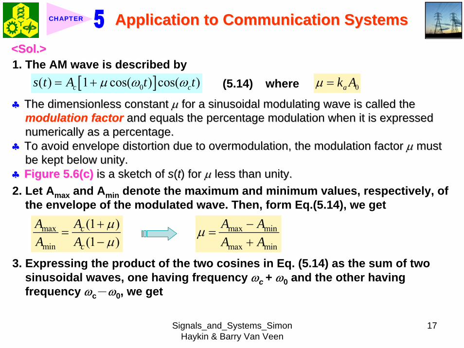
Signals_and_Systems_Simon Haykin amp Barry Van Veen
19
Application to Communication SystemsApplication to Communication SystemsCHAPTER
2 In either case the average power delivered to a 1-ohm load resistor by s(t) is composed of three components whose values are derived from Eq (115) asfollows
1 22
1 2 281 2 28
Carrier power
Upper side- frequency power
Lower side- frequency power
c
c
c
A
A
A
μ
μ
=
=
=
3 The ratio of the total sideband power to the total power in the modulated wave is therefore equal th μ 2(2 + μ 2) which depends only on the modulationfactor μ If μ = 1 (ie if 100 modulation is used) the total power in the twoside frequencies of the resulting AM wave is only one-third of the total powerin the modulated wave
4 Figure 57Figure 57 shows the percentage of total power in both side frequencies and in the carrier plotted against the percentage modulation
Signals_and_Systems_Simon Haykin amp Barry Van Veen
20
Application to Communication SystemsApplication to Communication SystemsCHAPTER
Figure 57 (p 437)Figure 57 (p 437)Variations of carrier power and side-frequency power with percentage modulation of AM wave for the case of sinusoidal modulation
546 546 Spectral OverlapSpectral Overlap1 When ωc lt ωm the modulated signal
s(t) undergoes frequency distortiondue to spectral overlap
Fig 58Fig 58clubs Assume that S(jω) is real valued2 The spectral overlap is produced by two movements
1)1) Movement of the lower sideband into the negative frequency rangeMovement of the lower sideband into the negative frequency range2)2) Movement of the image of the lower sideband into the positive frMovement of the image of the lower sideband into the positive frequency rangeequency range
3 For avoiding the spectral overlap problem the necessary condition is
c mω ωge
Signals_and_Systems_Simon Haykin amp Barry Van Veen
21
Application to Communication SystemsApplication to Communication SystemsCHAPTER
Figure 58 (p 438)Figure 58 (p 438)Spectral overlap phenomenon in amplitude modulation The phenomenon arises when the carrier frequency ωc is less than the highest frequency component ωm of the modulating signal
v equiv ω p equiv π
547 547 Demodulation of AM WaveDemodulation of AM Wave1 The envelope detector provides a simple yet effective device for the
demodulation of a narrowband AM signal for which the percentage modulation is less than 100
clubsclubs Narrowband means that the carrier is large compared with the mesNarrowband means that the carrier is large compared with the message bandwidthsage bandwidth2 Circuit diagram of an envelope detector Fig 59Fig 59
1) 1) The diode is ideal presenting zero impedance to current flow inThe diode is ideal presenting zero impedance to current flow in the forwardthe forward--biased region and infinite impedance in the reversebiased region and infinite impedance in the reverse--biased region biased region
Signals_and_Systems_Simon Haykin amp Barry Van Veen
22
Application to Communication SystemsApplication to Communication SystemsCHAPTER
Figure 59 (p 438)Figure 59 (p 438)Envelope detector illustrated by (a) circuit diagram (b) AM wave input and (c) envelope detector output assuming ideal conditions
Signals_and_Systems_Simon Haykin amp Barry Van Veen
23
Application to Communication SystemsApplication to Communication SystemsCHAPTER
2) 2) The AM signal applied to the envelope is supplied by a voltage sThe AM signal applied to the envelope is supplied by a voltage source of ource of internal resistance internal resistance RRss
3) The load resistance 3) The load resistance RRll is large compared with the source resistance is large compared with the source resistance RRss During Duringthe charging process the time constant is effectively equathe charging process the time constant is effectively equal to l to RRssCC This time This time constant must be short compared with the carrier period 2constant must be short compared with the carrier period 2ππωωcc that is that is
2s
c
R πω
ltlt (515)
3 The discharging time constant is equal to RlCRRllCC must be large such that the capacitor discharges slowly but notmust be large such that the capacitor discharges slowly but not so so large that the capacitor voltage will not discharge at the maximlarge that the capacitor voltage will not discharge at the maximum rate um rate of change of the modulating wave ieof change of the modulating wave ie2 2
lc m
R Cπ πω ω
ltlt ltlt (516) ωm equiv message
bandwidth
clubs Output ripple can be removed by low-pass filter
Signals_and_Systems_Simon Haykin amp Barry Van Veen
24
Application to Communication SystemsApplication to Communication SystemsCHAPTER
55 55 Double SidebandDouble Sideband--Suppressed ModulationSuppressed Modulation1 In full AM carrier wave c(t) is completely independent of the message signal
m(t)
Transmission of carrier wave A waste of power
2 To overcome this shortcoming we may suppress the carrier component from the modulated wave resulting in double sideband-suppressed carrier(DSB-SC) modulation
3 DSB-SC modulated signal( ) ( ) ( ) cos( ) ( )c cs t c t m t A t m tω= = (517)
clubs This modulated signal undergoes a phase reversal whenever the messagesignal m(t) crosses zero as illustrated in Fig 510Fig 510(a)(a) Message signal Message signal (b)(b) DSBDSB--SC modulated wave resulting from multiplication of the message SC modulated wave resulting from multiplication of the message
signal by the sinusoidal carrier wave signal by the sinusoidal carrier wave
Signals_and_Systems_Simon Haykin amp Barry Van Veen
25
Application to Communication SystemsApplication to Communication SystemsCHAPTER
Figure 510 (p 440)Figure 510 (p 440)Double-sideband-suppressed carrier modulation (a) Message signal (b) DSB-SC modulated wave resulting from multiplication of the message signal by the sinusoidal carrier wave
551 551 FrequencyFrequency--Domain DescriptionDomain Description1 Fourier transform of modulated signal s(t)
1( ) [ ( ( )) ( ( ))]2 c c cS j A M j M jω ω ω ω ω= minus + + (518)
where M(jω) equiv Fourier transform of m(t) minus ωm le ω le ωmFig 511 (a) and (b)Fig 511 (a) and (b)
Signals_and_Systems_Simon Haykin amp Barry Van Veen
26
Application to Communication SystemsApplication to Communication SystemsCHAPTER
Figure 511 (p 441)Figure 511 (p 441)Spectral content of DSB-SC modulated wave (a) Magnitude spectrum of message signal (b) Magnitude spectrum of DSB-SC modulated wave consisting of upper and lower sidebands only
v equiv ω p equiv π
clubs The modulation process simply translates the spectrum of the message signal by plusmn ωc
clubs Transmission bandwidth = 2 ωm2 A device for achieving DSB-SC is called a product modulator or simply
multiplierFig 512 (a)Fig 512 (a) shows the block diagram of a product modulator
Signals_and_Systems_Simon Haykin amp Barry Van Veen
27
Application to Communication SystemsApplication to Communication SystemsCHAPTER
Figure 512 (p 441)Figure 512 (p 441)(a) Product modulator for generating the DSB-SC modulated wave (b) Coherent detector for demodulation of the DSB-SC modulated wave
v equiv ω p equiv π
552 552 Coherent DetectionCoherent Detection1 The message signal m(t) may be recovered from DSB-SC
Fig 512 (b)Fig 512 (b)ss((tt) ) timestimes locally generated sinusoidal wave = locally generated sinusoidal wave = vv((tt))vv((tt) filtered by a Low) filtered by a Low--pass filterpass filter
Local oscillator
2 The local oscillator should be exactly coherent or synchronized in both frequency and phase with the carrier wave c(t)
Signals_and_Systems_Simon Haykin amp Barry Van Veen
28
Application to Communication SystemsApplication to Communication SystemsCHAPTER
Coherent detection or synchronization demodulation3 Derivation for coherent detection
1) Local oscillator cos(ωct + φ )2) Product modulator output
( ) cos( ) ( )cos( ) cos( ) ( )
1 1cos( ) ( ) cos(2 ) ( )2 2
c
c c c
c c c
v t t s tA t t m t
A m t A t m t
ω φω ω φ
φ ω φ
= += +
= + +(519)
1 cos( ) ( )2 cA m tφ
1 cos(2 ) ( )2 c cA t m tω φ+
A scaled version of the original message signal m(t)
DSBDSB--SC modulated signal with carrier SC modulated signal with carrier frequency 2 frequency 2 ωωcc
3) Magnitude spectrum Fig 5134) To clear separate two component of v(t) the original carrier frequency ωc
must satisfy the condition
Signals_and_Systems_Simon Haykin amp Barry Van Veen
29
Application to Communication SystemsApplication to Communication SystemsCHAPTER
Figure 513 (p 442)Figure 513 (p 442)Magnitude spectrum of the product modulator output v(t) in the coherent detector of Fig 512(b)
v equiv ω p equiv π
2 c m mω ω ωminus gt c mω ωgt (520) ωωmm equivequiv message bandwidthmessage bandwidth
4 Specification of low-pass filter1) 1) The cutoff frequency must be The cutoff frequency must be ωωm m 2) The transition band must be 2) The transition band must be ωωm m ≦≦ ωω ≦≦ ωωc c ωωm m
Thus the overall output in Thus the overall output in Fig 512(b)Fig 512(b) is given byis given by1( ) cos( ) ( )2o cv t A m tφ= (521)
cosφ equiv attenuation factor
Signals_and_Systems_Simon Haykin amp Barry Van Veen
30
Application to Communication SystemsApplication to Communication SystemsCHAPTER
5 (1) Demodulated signal vo(t) is proportional to m(t) when the error phase φis a constant
(2) Demodulated signal is maximum when φ = 0 and has a minimum zero when φ = plusmn π2
Example 53 Sinusoidal DSB-SC ModulationConsider again the sinusoidal modulating signal
0 0( ) cos( )m t A tω=
( ) cos( )c cc t A tω=with amplitude A0 and frequency ω0 see Fig 514(a) The carrier wave is
with amplitude Ac and frequency ωc see Fig 514(b) Investigate the time-domain and frequency-domain characteristics of the corresponding DSB-SC modulated waveltltSolgtSolgt
clubs φ = plusmn π2 represents the quadrature null effect of the coherent detector
1 The modulated DSB-SC signal is defined by
0 0
0 0 0 0
( ) cos( ) cos( )1 1cos[( ) ] cos[( ) ]2 2
c c
c c c c
s t A A t t
A A t A A t
ω ω
ω ω ω ω
=
= + + minus
Signals_and_Systems_Simon Haykin amp Barry Van Veen
31
Application to Communication SystemsApplication to Communication SystemsCHAPTER
2 The Fourier transform of s(t) is given by
0 0 0
0 0
1( ) cos[ ( ) ( )]2
( ) ( )
c c c
c c
S j A Aω π δ ω ω ω δ ω ω ω
δ ω ω ω δ ω ω ω
= minus minus + + +
+ minus + + + minus
which consists of four weighted impulse functions at the frequencies ωc+ ω0-ωc- ω0 ωc- ω0 and- ωc+ ω0 as illustrated in the right-hand side of Fig Fig 514(c)514(c)
3 This Fourier transform differs from that depicted in the right-hand side of Fig Fig 56(c)56(c) for the corresponding example of full AM in one important respect The impulse functions at plusmn ωc due to the carrier are removed
4 Application of the sinusoidally modulated DSB-SC signal to the product modulator of Fig 512(b) yields the output (assuming φ = 0)
0 0 0
0 0 0 0 0
1( ) cos( ) cos[( ) ] cos[( ) ]21 cos[(2 ) ] cos( ) cos[(2 ) ] cos( )4
c c c c
c c c
v t A A t t t
A A t t t t
ω ω ω ω ω
ω ω ω ω ω ω
= + + minus
= + + + minus +
Signals_and_Systems_Simon Haykin amp Barry Van Veen
32
Application to Communication SystemsApplication to Communication SystemsCHAPTER
Figure 514 (p Figure 514 (p 443)443)Time-domain (on the left) and frequency-domain (on the right) characteristics of DSB-SC modulation produced by a sinusoidal modulating wave (a) Modulating wave (b) Carrier wave (c) DSB-SC modulated wave Note that ω= 2πƒ
v equiv ω p equiv π
Signals_and_Systems_Simon Haykin amp Barry Van Veen
33
Application to Communication SystemsApplication to Communication SystemsCHAPTER
5 The first two sinusoidal terms of v(t) are produced by the upper side frequency and the last two sinusoidal terms are produced by the lower side frequency
6 With ωcgt ω0 the first and third sinusoidal terms of frequencies 2ωc+ ω0 and 2ωc-ω0 respectively are removed by the low-pass filter of Fig 512(b)Fig 512(b) which leaves the second and fourth sinusoidal terms of frequency ω0 as the only output of the filter The coherent detector output thus reproduces the original modulating wave
7 Note however that this output appears as two equal terms one derived from the upper side frequency and the other from the lower side frequency We therefore conclude that for the transmission of the sinusoidal signal A0 cos(ω0t) only one side frequency is necessary (The issue will be discussed further in Section 57Section 57)
553 553 CostasCostas ReceiverReceiver1 Costas receiver Fig 515Fig 5152 This receiver consists of two coherent detector supplied with the same input
ie the incoming DSB-Sc wave
cos(2 ) ( )c cA f t m tπ but with individual local oscillator signals that are in phase duadrature with respect to each other
In-phase coherent detector (I-Channel) and quadrature-phase coherent detector (Q-Channel)
Signals_and_Systems_Simon Haykin amp Barry Van Veen
34
Application to Communication SystemsApplication to Communication SystemsCHAPTER
Figure 515 (p 445)Figure 515 (p 445)Costas receiver
v equiv ω p equiv π
Signals_and_Systems_Simon Haykin amp Barry Van Veen
35
Application to Communication SystemsApplication to Communication SystemsCHAPTER
56 56 QuadratureQuadrature--Carrier MultiplexingCarrier Multiplexing
Figure 516 (p 446)Figure 516 (p 446)Quadrature-carrier multiplexing system exploiting the quadrature null effect (a) Transmitter (b) Receiver assuming perfect synchronization with the transmitter
v equiv ω p equiv π
1 1 A A quadraturequadrature--carrier multiplexing or carrier multiplexing or quadraturequadrature--amplitude modulation (QAM) amplitude modulation (QAM) system enables two DSBsystem enables two DSB--SC modulated waves to occupy the same transmission SC modulated waves to occupy the same transmission bandwidth and yet it allows for their separation at the receivebandwidth and yet it allows for their separation at the receiver outputr output
BandwidthBandwidth--conservation schemeconservation scheme
Signals_and_Systems_Simon Haykin amp Barry Van Veen
36
Application to Communication SystemsApplication to Communication SystemsCHAPTER
2 Fig 5-16(a) Block diagram of the quadrature-carrier multiplexing systemFig 5-16(a) transmitter Fig 5-16(b) receiver
3 Multiplexed signal s(t)
(522) 1 2( ) ( ) cos( ) ( )sin( )c c c cs t A m t t A m t tω ω= +
where m1(t) and m2(t) denotes the two different message signals applied to the product modulations
clubsTransmission bandwidth = 2 ωm centered at ωc where ωm is the commonmessage bandwidth of m1(t) and m2(t)
4 The output of the top detector at receiver is 1
12 ( )cA m t
The output of the bottom detector at receiver is1
22 ( )cA m t
57 57 Other Variants of Amplitude Modulation Other Variants of Amplitude Modulation clubs Basic concept Full AM and DSB-SC rArr Wasteful of bandwidthclubs Given the amplitude and phase spectra of either lower or upper sideband
we can uniquely determine the other
Signals_and_Systems_Simon Haykin amp Barry Van Veen
37
Application to Communication SystemsApplication to Communication SystemsCHAPTER
clubs Single-sideband (SSB) modulation only one sideband is transmitted571 571 FrequencyFrequency--Domain Description of SSB ModulationDomain Description of SSB Modulation1 Consider a message signal m(t) with a spectrum M(jω) limited to the band
ωa le ω le ωb Fig 5-17 (a)2 DSB-SC modulated signal
( ) cos( )c cm t A tωtimes Fig 5-17 (b)
3 (1) Upper sideband the frequencies above ωc and below minus ωc(2) Upper sideband the frequencies below ωc and above minus ωc
Fig 5-17 (c)4 When only the lower sideband is transmitted the spectrum of the
corresponding SSB modulated wave is as shown in Fig 5-17 (d) 5 Advantages of SSB
(1) Reduced bandwidth requirement(2) Elimination of the high-power carrier waveDisadvantage od SSB(1) Cost and complexity of implementing both the transmitter and receiver
Signals_and_Systems_Simon Haykin amp Barry Van Veen
38
Application to Communication SystemsApplication to Communication SystemsCHAPTER
Figure 517 Figure 517 (p 447)(p 447)Frequency-domain characteristics of SSB modulation (a) Magnitude spectrum of message signal with energy gap from ndash ωa to ωa
(c) Magnitude spectrum of SSB modulated wave containing upper sideband only
(d) Magnitude spectrum of SSB modulated wave containing lower sideband only
(b) Magnitude spectrum of DSB-SC signal
v equiv ω p equiv π
Signals_and_Systems_Simon Haykin amp Barry Van Veen
39
Application to Communication SystemsApplication to Communication SystemsCHAPTER
6 Frequency-discrimination scheme for producing SSB modulation Fig 518clubs Bandpass filter is designed to pass the sideband selected for transmission
and suppress the remaining sidebandclubs Requirement in SSB signal the message signal applied to the product
modulator must have a energy gap in its spectrum Refer to Fig 517 (a)
Figure 518 (p 448)Figure 518 (p 448)System consisting of product modulator and bandpass filter for generating SSB modulated wave
v equiv ω p equiv π
572 572 TimeTime--Domain Description of SSB ModulationDomain Description of SSB Modulation1 Mathematical tool Hilbert transform
The Hilbert transform of a signal x(t) is defined by1 ( ) 1ˆ( ) ( )xx t d x t
t tτ τ
π τ πinfin
minusinfin= = lowast
minusint
Signals_and_Systems_Simon Haykin amp Barry Van Veen
40
Application to Communication SystemsApplication to Communication SystemsCHAPTER
The Fourier transform of 1(πt) is minus j times the signum function denoted
1 for 0sgn( ) 0 for 0
1 for 0
ωω ω
ω
+ gt⎧⎪= =⎨⎪minus lt⎩
2 Passing x(t) through a Hilbert transformer is equivalent to the combination of the following two operations in frequency domain1) Keeping X(jω)unchanged for all ω 2) Shifting areX(jω) (ie the phase spectrum of x(t)) by +90deg for negative
frequencies and minus 90deg for positive frequencies clubs Hilbert transformer = Wideband minus 90deg phase shifter 573 573 Vestigial Sideband ModulationVestigial Sideband Modulation1 When the message signal contains significant components at extremely
low frequencies the upper and lower sidebands meet at the carrier frequency
Using SSB is inappropriateUsing SSB is inappropriateEx TV signals or
wideband dataUsing VSB (Vestigial sideband) modulation is appropriateUsing VSB (Vestigial sideband) modulation is appropriate
Signals_and_Systems_Simon Haykin amp Barry Van Veen
41
Application to Communication SystemsApplication to Communication SystemsCHAPTER
2 VSB is a compromise between SSB and DSB-SC forms of modulationIn VSB modulation one sideband is passes almost completely whereas just a trace or vestige of the other sideband is retained
3 Fig 519 illustrates a VSB modulated wave s(t) in relation to the message signal m(t)
v equiv ω p equiv π
Figure 519 (p 449)Figure 519 (p 449)Spectral content of VSB modulated wave (a) Magnitude spectrum of message signal (c) Magnitude spectrum of VSB modulated wave containing a vestige of the lower sideband
clubs The lower sideband is modified into the vestigial sideband4 Transmission bandwidth of VSB modulated wave T m vω ω ω= + (523)
where ωm is the message bandwidth and ωu is the width of the vestigial sideband
Signals_and_Systems_Simon Haykin amp Barry Van Veen
42
Application to Communication SystemsApplication to Communication SystemsCHAPTER
5 Generation of VSB modulated wave Fig 520
Figure 520 (p 450)Figure 520 (p 450)System consisting of product modulator and sideband shaping filter for generating VSB modulated wave
v equiv ω p equiv π
Passing a DSBPassing a DSB--SC modulated wave through a sidebandSC modulated wave through a sideband--shaping filtershaping filter6 The sideband-shaping filter is designed so that the original message
spectrum M(jω) is reproduced on the demodulation as a result of the superposition of two spectra
1) The positive-frequency part of S(jω) (ie the Fourier transform of the transmitted signal s(t)) shifted downward in frequency by ωc
2) The negative-frequency part of S(jω) shifted upward in frequency by ωc
Fig 521 A reflection of the vestige of the lower sideband makes up for the missing parts of the upper sideband
Signals_and_Systems_Simon Haykin amp Barry Van Veen
43
Application to Communication SystemsApplication to Communication SystemsCHAPTER
Figure 521 (p 450)Figure 521 (p 450)Superposition of the two spectra shown in parts (a) and (b) of the figure results in the original message spectrum (shown dashed) upon demodulation
58 58 PulsePulse--Amplitude Modulation Amplitude Modulation clubs Basic concept
Basic role in the operation of AM Frequency-shiftingBasic role in the operation of PAM Sampling
581 581 Sampling RevisitedSampling Revisited1 Sampling theorem
In view point of PAMIn view point of PAM
Signals_and_Systems_Simon Haykin amp Barry Van Veen
44
Application to Communication SystemsApplication to Communication SystemsCHAPTER
1) A band-limited signal of finite energy that has no radian frequency components higher than ωm is uniquely determined by the values of the signal at instants of time separated by π ωm seconds
2) A band-limited signal of finite energy that has no radian frequency components higher than ωm may be completely recovered from a knowledge of its samples taken at the rate of ωm π per seconds
clubs Part 1) rArr Be exploited in the transmitter of a PAM clubs Part 2) rArr Be exploited in the Receiver of a PAM2 To combat the effects of aliasing in practice we use two corrective measures1) Prior to sampling a low-pass antialiasing filter is used to attenuate those high-
frequency components of the signal which lie outside the band of interest2) The filtered signal is sampled at a rate slightly higher than the Nyquist rate3 Generation of a PAM signal Fig 522Fig 522Example 54 Telephonic CommunicationThe highest frequency component of a speech signal needed for telephonic communication is about 31 kHz Suggest a suitable value for the sampling rate ltltSolgtSolgt
Signals_and_Systems_Simon Haykin amp Barry Van Veen
45
Application to Communication SystemsApplication to Communication SystemsCHAPTER
Figure 522 (p 451)Figure 522 (p 451)System consisting of antialiasing filter and sample-and-hold circuit for converting a message signal into a flattopped PAM signal
1 The highest frequency component of 31 kHz corresponds to 362 10 radsmω π= times
Correspondingly the Nyquist rate is
62 kHzmωπ
=
2 A suitable value for the sampling rate-one slightly higher than the Nyquistrate-may be 8 kHz a rate that is the international standard for telephone speech signals
Signals_and_Systems_Simon Haykin amp Barry Van Veen
46
Application to Communication SystemsApplication to Communication SystemsCHAPTER
582 582 Mathematical Description of PAMMathematical Description of PAM1 The carrier wave used in PAM consists of a sequence of short pulses of
fixed duration in terms of which PAM is formally defined as followsPAM is a form of pulse modulation in which the amplitude of the PAM is a form of pulse modulation in which the amplitude of the pulsed carrier is pulsed carrier is varied in accordance with instantaneous sample values of the mesvaried in accordance with instantaneous sample values of the message signalsage signal the duration of the pulsed carrier is maintained constant throughout
Fig 523Fig 523
Figure 523 (p452) Figure 523 (p452) Waveform of flattopped PAM signal with pulse duration T0 and sampling period Ts
Signals_and_Systems_Simon Haykin amp Barry Van Veen
47
Application to Communication SystemsApplication to Communication SystemsCHAPTER
2 Mathematical representation of the PAM
( ) [ ] ( )sn
s t m n b t nTinfin
=minusinfin
= minussum (524) s(t) equiv PAM signal m(t) equiv
message signal
Ts equiv sampling period m[n] equiv the values of m(t) at t = nTs h(t) equiv rectangular pulse of the unit amplitude and duration T0
3 Rectangular pulse
01 0( )
0 otherwiset T
h tlt lt⎧
= ⎨⎩
(525) Fig 524 (a)Fig 524 (a)
clubs Eq (524) is a sample-and-hold operationAnalogous to zeroAnalogous to zero--orderorder--holdhold--
based reconstruction in Sec 46based reconstruction in Sec 46
差異差異hh((tt) ) 的的TTss與與TT00
4 Impulse-sampled version of message signal m(t)
( ) [ ] ( )sn
m t m n t nTδ δinfin
=minusinfin
= minussum (526)
5 PAM signal( ) [ ] ( )
( ) ( )
sn
s t m n b t nT
m t b tδ
infin
=minusinfin
= minus
=
sum(527)
Convolution of impulse-sampled version mδ(t) and h(t)
Time domain Time domain operationoperation
Signals_and_Systems_Simon Haykin amp Barry Van Veen
48
Application to Communication SystemsApplication to Communication SystemsCHAPTER
Figure 524 (p 453)(a) Rectangular pulse h(t) of unit amplitude and duration T0 (b) Magnitude spectrum |H(jω)| and phase spectrum argH(jω) of pulse h(t)
v equiv ω p equiv π
Signals_and_Systems_Simon Haykin amp Barry Van Veen
49
Application to Communication SystemsApplication to Communication SystemsCHAPTER
6 FT of PAM signal( ) ( ) ( )S j M j H jδω ω ω= (528)
where( ) ( )FTS j s tω larr⎯rarr ( ) ( )FTM j m tδ δω larr⎯rarr ( ) ( )FTH j h tω larr⎯rarr
7 Impulse sampling of the message signal m(t) introduces periodicity into the spectrum as given by
1( ) ( ( ))sks
M j M j kTδ ω ω ω
infin
=minusinfin
= minussum (529) 1Ts equiv sampling rate ωs = 2πTs rads
1( ) ( ( )) ( )sks
S j M j k H jT
ω ω ω ωinfin
=minusinfin
= minussum (530)
( ) ( )FTM j m tω larr⎯rarrwhere
clubs Suppose that m(t) is strictly band limited and that the sampling rate 1Ts is greater than the Nyquist rate Then passing s(t) through a reconstruction filter chosen as an ideal low-pass filter with cutoff frequency ωm and gain Ts we find that the spectrum of the resulting filter output is equal to M(jω)H(jω)
Signals_and_Systems_Simon Haykin amp Barry Van Veen
50
Application to Communication SystemsApplication to Communication SystemsCHAPTER
8 From Eq (525) we find that0 2
0 0( ) sin ( (2 )) j TH j T c T e ωω ω π minus= (531) Fig 524(b) magnitude and phase of H(jω)
clubs Using PAM to represent a continuous-time message signal we introduce amplitude distortion as well as a delay of T02
clubs The frequency distortion caused by the use of flat-topped sampled in the generation of a PAM wave illustrated in Fig 523Fig 523 is referred to as the aperture effect
583 583 Demodulation of PAM SignalDemodulation of PAM Signal1 Reconstruction scheme Fig 525Fig 525
Figure 525 (p 454)Figure 525 (p 454)System consisting of low-pass interpolation filter and equalizer for reconstructing a message signal from its flattopped sampled version
clubs The system consists of low-pass interpolation filter and equalizer connected in cascade
Signals_and_Systems_Simon Haykin amp Barry Van Veen
51
Application to Communication SystemsApplication to Communication SystemsCHAPTER
2 The cutoff frequency of low-pass filter = the highest frequency ωm of message signal
3 The equalizer is used to correct the aperture effect due to flat-topped sampling in the sample-and-hold circuit
4 The equalizer has the effect of decreasing the in-band loss of the interpolation filter as frequency increases in such a manner as to compensate for the aperture effect
5 Amplitude response of equalizer
0
0 0 0 0
1 1 1| ( ) | | sinc( 2) | 2 | sin( 2) |
TH j T T T T
ωω ω ω
= =
Frequency response Eq (531)
Example 55 Equalization for PAM TransmissionThe duty cycle in a PAM signal namely T0 Ts is 10 Evaluate the peak amplification required for equalizationltltSolgtSolgt1 At ωm = π Ts which corresponds to the highest frequency component of the
message signal for a sampling rate equal to the Nyquist rate we find from Eq (531) that the magnitude response of the equalizer at ωm normalized to that at zero frequency is
Signals_and_Systems_Simon Haykin amp Barry Van Veen
52
Application to Communication SystemsApplication to Communication SystemsCHAPTER
Figure 526 (p 455)Figure 526 (p 455)Normalized equalization (to compensate for aperture effect) plotted against the duty cycle T0Ts
Signals_and_Systems_Simon Haykin amp Barry Van Veen
53
Application to Communication SystemsApplication to Communication SystemsCHAPTER
0
0 0
( 2)( )1sin (05 ) sin[( 2)( )]
s
s s
T Tc T T T T
ππ
=
where the ratio T0 Ts is equal to the duty cycle of the sampling pulses 2 In Fig 526Fig 526 this result is plotted as a function of the duty cycle T0 Ts Ideally it
should be equal to unity for all values of T0 Ts 3 For a duty cycle of 10 it is equal to 10041 It follows that for duty cycles of less
than 10 the magnitude equalization required is less than 10041 in which case the aperture effect is usually considered to be negligible
59 59 Multiplexing Multiplexing clubs Three basic types of multiplexing1 Frequency-division multiplexing in which the signals are separated by
allocating them to different frequency bands This is illustrated in Fig 527(a) for the case of six different message signals Frequency-division multiplexing favors the use of CW modulation where each message signal is able to use the channel on a continuous-time basis
2 Time-division multiplexing wherein the signals are separated by allocating them to different time slots within a sampling interval
Signals_and_Systems_Simon Haykin amp Barry Van Veen
54
Application to Communication SystemsApplication to Communication SystemsCHAPTER
This second type of multiplexing is illustrated in Fig 527(b) for the case of six different message signals Code-division multiplexing which relies on the assignment of different codes to the individual users of the channel
3 Code-division multiplexing which relies on the assignment of different codes to the individual users of the channel
591 591 FrequencyFrequency--Domain Multiplexing (FDM)Domain Multiplexing (FDM)1 Block diagram Fig 528Fig 5282 Incoming message signals low-pass variety3 Low-pass filter to remove high-frequency components such that the signal
in each channel does not disturb each other4 MOD (modulator) shift the frequency ranges of the signals so as to occupy
mutually exclusive frequency intervalsSSB is often used in this stageEx Voice input is usually assigned a bandwidth of 4 kHz
5 Band-pass filters are used to restrict the band of each modulated wave to its prescribed range
6 Band-pass filters in receiver separate the message signals7 DEM (demodulator) to recover signalsclubs FDM in Fig 528 operates in only one direction
Signals_and_Systems_Simon Haykin amp Barry Van Veen
55
Application to Communication SystemsApplication to Communication SystemsCHAPTER
Figure 527 (p 456)Figure 527 (p 456)Two basic forms of multiplexing (a) Frequency-division multiplexing (with guardbands) (b) Time-division multiplexing no provision is made here for synchronizing pulses
Signals_and_Systems_Simon Haykin amp Barry Van Veen
56
Application to Communication SystemsApplication to Communication SystemsCHAPTER
Figure 528 (p 457)Figure 528 (p 457)Block diagram of FDM system showing the important constituents of the transmitter and receiver
Signals_and_Systems_Simon Haykin amp Barry Van Veen
57
Application to Communication SystemsApplication to Communication SystemsCHAPTER
Example 56 SSB-FDM System
ltltSolgtSolgt
An FDM system is used to multiplex 24 independent voice signals SSB modulation is used for the transmission Given that each voice signal is allotted a bandwidth 4kHz calculate the overall transmission bandwidth of the channel
With each voice signal allotted a bandwidth of 4 kHz the use of SSB modulation requires a bandwidth of 4 kHz for its transmission Accordingly the overall transmission bandwidth provided by the channel is 24 X 4 = 96 kHz 592 592 TimeTime--Domain Multiplexing (TDM)Domain Multiplexing (TDM)clubs Basic to the operation of a TDM system is the sampling theoremclubs The transmission of the message samples engages the transmission channel for
only a fraction of the sampling interval on a periodic basis equal to the width T0 of a PAM modulating pulse
1 Block diagram Fig 529Fig 5292 Commutator is usually implemented by means of electronic switching
circuitry3 The function of commutator is two folds
Signals_and_Systems_Simon Haykin amp Barry Van Veen
58
Application to Communication SystemsApplication to Communication SystemsCHAPTER
Figure 529 (p 458)Figure 529 (p 458)Block diagram of TDM system showing the important constituents of the transmitter and receiver
(1) To take a narrow sample of each of the M input message signals at a rate 1Tsthat is slightly higher than ωcπ where ωc is the cutoff frequency of the input low-pass filter
(2) To sequentially interleave these M samples inside a sampling interval Ts4 Pulse modulator transform the multiplexed signal into a form suitable for
transmission over the common channel
Signals_and_Systems_Simon Haykin amp Barry Van Veen
59
Application to Communication SystemsApplication to Communication SystemsCHAPTER
clubs The use of time-division multiplexing introduces a bandwidth expansion factor M because the scheme must squeeze M samples derived from M independent message sources into a time slot equal to one sampling interval
5 Pulse demodulator performs the inverse operation of the pulse modulator6 Decommutator distributes the narrow samples produced by pulse demodulator to the appropriate low-pass reconstruction filter7 Synchronization between the timing operations of the transmitter and
receiver in a TDM system is essential for satisfactory performance of the system
Inserting an extra pulse into each sampling interval on a regular basisBandwidth expansion factor is increased to M + 1
clubs The TDM system is hghly sensitive to the dispersion in the common transmission channel
Example 57 Comparison of TDM with FDMATDM system is used to multiplex four independent voice signals using PAM Each voice signal is sampled at the rate of 8 kHz The system incorporates a synchronizing pulse train for its proper operation
Signals_and_Systems_Simon Haykin amp Barry Van Veen
60
Application to Communication SystemsApplication to Communication SystemsCHAPTER
(a) Determine the timing relationships between the synchronizing pulse train and the impulse trains used to sample the four voice signals
(b) Calculate the transmission bandwidth of the channel for the TDM system and compare the result with a corresponding FDM system using SSBmodulation
ltltSolgtSolgt(a) The sampling period is
31 125 s
8 10sT s μ= =times
In this example the number of voice signals is M = 4 Hence dividing the sampling period of 125 μs among these voice signals and the synchronizing pulse train we obtain the time slot allocated to each one of them
0 1125 25 s
5
sTTM
μ
=+
= =
Signals_and_Systems_Simon Haykin amp Barry Van Veen
61
Application to Communication SystemsApplication to Communication SystemsCHAPTER
Figure 530Figure 530 shows the timing relationships between the synchronizing pulse train and the four impulse trains used to sample the different voice signals in a single frame Each frame includes time slots of common duration T0 = 25 μs which are allocated to the pulse-modulated signals and synchronizing pulse
Figure 530 (p 459)Figure 530 (p 459)Composition of one frame of a multiplexed PAM signal incorporating four voice-signals and a synchronizing pulse
Signals_and_Systems_Simon Haykin amp Barry Van Veen
62
Application to Communication SystemsApplication to Communication SystemsCHAPTER
(b) As a consequence of the time-bandwidth product (see Section 317) there is an inverse relationship between the duration of a pulse and the bandwidth (ie cutoff frequency) of the channel needed for itstransmission Accordingly the overall transmission bandwidth of the channel is
0
21 1 MHz 40 kHz
25
TTf
T
ωπ
=
= = =
In contrast the use of an FDM system based on SSB modulation requires a channel bandwidth equal to M times that of a single voice signal-that is 4 X 4 = 16 kHz Thus the use of PAM-TDM requires a channel bandwidth that is 40 16 = 25 times that of SSB-FDMIn practice pulse-code modulation is commonly used as the method of modulation for TDM this results in a further increase in channel bandwidth depending on the length of the code word used in the digital representation of each pulse in the PAM signal
Signals_and_Systems_Simon Haykin amp Barry Van Veen
63
Application to Communication SystemsApplication to Communication SystemsCHAPTER
510 510 Pulse and Group Delays Pulse and Group Delays 1 Whenever a signal is transmitted through a dispersive (ie frequency
selective) system some delay is introduced into the output signal in relation to the input signal
2 The delay is determined by the phase response of the system3 Phase response of a dispersive communication channel
( ) arg ( )H jφ ω ω= (532)
A signal is transmitted through the channel at a frequency ωc The signal received at the channel lags the transmitted signal by φ(ωc) The time delay is called phase delay formally defined as
( )cp
c
φ ωτω
= minus (533)
The phase delay is not necessarily the true signal delayclubs Case study for DSB-SC1 Transmitted signal
0( ) cos( ) cos( )cs t A t tω ω= (534)
ωc equiv carrier frequency ω0 equiv sinusoidal modulation frequency
A = AcA0
Signals_and_Systems_Simon Haykin amp Barry Van Veen
64
Application to Communication SystemsApplication to Communication SystemsCHAPTER
1 21 1( ) cos( ) cos( )2 2
s t A t A tω ω= +
1 0cω ω ω= + (535) where
2 0cω ω ω= minus (536)
Upper frequency
Lower frequency
2 Let the s(t) be transmitted through the channel with phase response φ (ω) Accordingly the signal received at the channel output is
1 1 2 21 1( ) cos( ( )) cos( ( ))2 2
y t A t A tω φ ω ω φ ω= + + +
1 2 1 20
( ) ( ) ( )1 ( )( ) cos cos2 2cy t A t tφ ω φ ω φ ω φ ωω ω+⎛ ⎞ ⎛ ⎞= + +⎜ ⎟ ⎜ ⎟
⎝ ⎠ ⎝ ⎠(537)
3 Two observations from Eq (537)1) The carrier component at frequency ωc in y(t) lags its counterpart in s(t) by
frac12 (φ (ω1) + φ (ω2)) which represents a time delay equal to
1 2 1 2
c 1 2
( )+ ( ) ( )+ ( )2 +
φ ω φ ω φ ω φ ωω ω ω
minus = minus (538)
Signals_and_Systems_Simon Haykin amp Barry Van Veen
65
Application to Communication SystemsApplication to Communication SystemsCHAPTER
2) The message component at frequency ω0 in y(t) lags its counterpart in s(t) by frac12 (φ (ω1) minus φ (ω2)) which represents a time delay equal to
1 2 1 2
0 1 2
( ) ( ) ( ) ( )2
φ ω φ ω φ ω φ ωω ω ωminus minus
minus = minusminus
(539)
4 Suppose that ω0 lt ωc rArr the side frequencies are close together with ω c between them Such a modulated signal is said to be a narrowband signal The phase response φ (ω) in the vicinity of ω = ωc is approximated by two-term Taylor series expansion
( )( ) ( ) ( )c
c cd
d ω ω
φ ωφ ω φ ω ω ωω =
= + times minus (540)
Phase delay = ( ) c cφ ω ωminus
5 The time delay introduced by the message signal (ie he ldquoenveloperdquo of the modulated signal) is given by
( )
c
gd
d ω ω
φ ωτω =
= minus (541) The time delay τg is called the
envelope delay or group delay
Signals_and_Systems_Simon Haykin amp Barry Van Veen
66
Application to Communication SystemsApplication to Communication SystemsCHAPTER
6 When a modulated signal is transmitted through a communication channel there are two different delays to be considered1) The carrier or phase delay τp defined by Eq (533)2) The envelope or group delay τg defined by Eq (541)
clubs The group delay is the true signal delay
Example 58 Phase and Group Delays for Ban-pass Channel
ltltSolgtSolgt
The phase response of a band-pass communication channel is defined by 2 2
1( ) tan c
c
ω ωφ ωωω
minus ⎛ ⎞minus= minus ⎜ ⎟
⎝ ⎠The signal s(t) defined in Eq (534) is transmitted through this channel with
475 radscω = 0 025 radsω =andCalculate (a) the phase delay and (b) the group delay
(a) At ω = ωc φ (ωc) = 0 According to Eq (533) the phase delay τ p is zero (b) Differentiating φ (ω) with respect to ω we get
Signals_and_Systems_Simon Haykin amp Barry Van Veen
67
Application to Communication SystemsApplication to Communication SystemsCHAPTER
2 2
2 2 2 2 2
( )( )( )
c c
c c
dd
ω ω ωφ ωω ω ω ω ω
+= minus
+ minus
Using thing result in Eq (541) we find that the group delay is 2 2 04211
475gc
sτω
= = =
1 One waveform shown as a solid curve was obtained by multiplying the transmitted signal s(t) by the carrier wave cos(ωct)
2 The second waveform shown as a dotted curve was obtained by multiplying the received signal y(t) by the carrier wave cos(ωct)
To display the results obtained in parts (a) and (b) in graphical form Fig 531Fig 531shows a superposition of two waveforms obtained as follows
The figure clearly shows that the carrier (phase) delay τ p is zero and the envelope of the received signal y(t) is lagging behind that of the transmitted signal by τs seconds For the presentation of waveforms in this figure we purposely did not use a filter to suppress the high frequency components resulting from the multiplications described under points 1 and 2 because of the desire to retain a contribution due to the carrier for display
Signals_and_Systems_Simon Haykin amp Barry Van Veen
68
Application to Communication SystemsApplication to Communication SystemsCHAPTER
Figure 531 Figure 531 (p 463)(p 463)Highlighting the zero carrier delay (solid curve) and group delay τg (dotted curve) which are determined in accordance with Example 58
Signals_and_Systems_Simon Haykin amp Barry Van Veen
69
Application to Communication SystemsApplication to Communication SystemsCHAPTER
clubs Not also that the separation between the upper side frequency ω1 = ωc + ω0 = 500 rads and the lower side frequency ω2 = ωc minus ω0 = 450 rads is about 10 of the carrier frequency ωc = 475 rads which justifies referring to the modulated signal in this example as a narrowband signal
5101 5101 Some Practical ConsiderationsSome Practical Considerationsclubs What is the practical importance of group delay 1 Eq (541) for determining group delay applies strictly to narrowband
modulated signal2 The message bandwidth may be comparable to the carrier frequency In
this situation the group delay is formulated as a frequency-dependent parameter ie ( )d( )g d
φ ωτ ωω
= minus (542)
3 When a wideband modulated signals transmitted through a dispersive channel the frequency components of the message signal are delayed by different amounts at the channel output
Delay distortionFig 532Fig 532 Group delay response of voice-grade telephone channel
Signals_and_Systems_Simon Haykin amp Barry Van Veen
70
Application to Communication SystemsApplication to Communication SystemsCHAPTER
Figure 532 (p 464)Group delay response of voice-grade telephone channel (Adapted from J C Bellamy Digital Telephony Wiley 1982)
511 511 Exploring Concepts with MATLABExploring Concepts with MATLAB5111 5111 Full AMFull AMclubs Sinusoidal modulation
clubs To reconstruct a faithful version of the original message signal in the receiver we have to use a delay equalizer
0( ) [1 cos( )]cos( )c cs t A t tμ ω ω= +1 AM experiment
1cA =
08 radscω π= 0 01 radsω π=Carrier amplitude
Carrier frequency Modulation amplitude
Signals_and_Systems_Simon Haykin amp Barry Van Veen
71
Application to Communication SystemsApplication to Communication SystemsCHAPTER
2 We wish to display and analyze 10 full cycles of the AM wave corresponding to a total duration of 200 s Choosing a sampling rate 1Ts = 10 Hz we have a total of N = 2000 time samples The frequency band of interest is minus 10 π ≦ ω ≦ 10 π Since the separation between the carrier and either side frequency is equal to the modulation frequency ω0 = 01 π rads we would like to have a frequency resolution ωr = 001π rads To achieve this resolution we require the following number of frequency samples (see Eq (442))
20 2000001
s
r
M ω πω π
ge = =
3 We therefore choose M = 2000 To approximate the Fourier transform of the AM wave s(t) we may use a 2000-point DTFS The only variable in the AM experiment is the modulation factor μ with respect to which we wish to investigate three different situationsμ = 05 corresponding to under-modulationμ = 10 for which the AM system is on the verge of over-modulationμ = 20 corresponding to over-modulation
Signals_and_Systems_Simon Haykin amp Barry Van Veen
72
Application to Communication SystemsApplication to Communication SystemsCHAPTER
4 MATLAB commandsAc = 1 carrier amplitudewc = 08pi carrier frequencyw0 = 01pi modulation frequencymu = 05 modulation factort = 0011999s = Ac(1 + mucos(w0t))cos(wct)plot(ts)Smag = abs(fftshift(fft(s2000)))2000 Smag denotes the magnitude specturm of the AM wavew = 10[-1000999]2pi2000plot(wSmag)axis ([-30 30 0 08])
5 5 μμ = 05 = 05 case case Fig 533Fig 533μμ = 10 case = 10 case Fig 534Fig 534μμ = 20 case = 20 case Fig 535Fig 535
Discussion see pp 466-469 textbook
Signals_and_Systems_Simon Haykin amp Barry Van Veen
73
Application to Communication SystemsApplication to Communication SystemsCHAPTER
-30 -20 -10 0 10 20 300
02
04
06
0 50 100 150 200-2
-1
0
1
2
2 22 24 26 28 3
02
04
06
(a) Time (s)
Time domain
Frequency domain
(b) Frequency (rads)
Frequency domain
Frequency (rads)
Figure 533 (p 466)Amplitude modulation with 50 modulation (a) AM wave (b) magnitude spectrum of the AM wave and (c) expanded spectrum around the carrier frequency
μμ = 05 = 05 casecase
Signals_and_Systems_Simon Haykin amp Barry Van Veen
74
Application to Communication SystemsApplication to Communication SystemsCHAPTER
Figure 534 (p 467)Figure 534 (p 467)Amplitude modulation with 100 modulation (a) AM wave (b) magnitude spectrum of the AM wave and (c) expanded spectrum around the carrier frequency
Signals_and_Systems_Simon Haykin amp Barry Van Veen
75
Application to Communication SystemsApplication to Communication SystemsCHAPTER
Figure 535 (p 468)Amplitude modulation with 200 modulation (a) AM wave (b) magnitude spectrum of the AM wave and (c) expanded spectrum around the carrier frequency
Signals_and_Systems_Simon Haykin amp Barry Van Veen
76
Application to Communication SystemsApplication to Communication SystemsCHAPTER
5112 5112 DSBDSB--SC ModulationSC Modulation1 Sinusoidal modulation
0 0( ) cos( ) cos( )c cs t A A t tω ω=
2 MATLAB commands
Ac = 1 carrier amplitudewc = 08pi carrier frequency in radsA0 = 1 amplitude of modulating signalw0 = 01pi frequency of modulating signalt = 011999s = AcA0cos(wct)cos(w0t)plot(ts)Smag = abs(fftshift(fft(s2000)))2000w = 10[-1000999]2pi2000plot(wSmag)
3 3 DSBDSB--SC modulated waveSC modulated wave Fig 536Fig 536 Discussion see pp 466-469 textbook
4 Output of the product modulator in Fig 512 (b) with φ = 0
Signals_and_Systems_Simon Haykin amp Barry Van Veen
77
Application to Communication SystemsApplication to Communication SystemsCHAPTER
Figure 536 (p 469)DSB-SC modulation (a) DSB-SC modulated wave (b) magnitude spectrum of the modulated wave and (c) expanded spectrum around the carrier frequency
Signals_and_Systems_Simon Haykin amp Barry Van Veen
78
Application to Communication SystemsApplication to Communication SystemsCHAPTER
( ) ( ) cos( )cv t s t tω=
5 MATLAB commandsgtgt v = scos(wct)
6 Fig 537 (a) waveforms of v(t) Fig 537 (b) magnitude spectrum which readily shows that v(t) consists of the following components1) A sinusoidal component with frequency 01π rads representing the
modulating wave2) A new DSB-SC modulated wave with double carrier frequency of 16π rads
in actuality the side frequencies of this modulated wave are located at 15πand 17π rads
1) The frequency of the modulating wave lies inside the passband of the filter2) The upper and lower side frequencies of the new DSB-SC modulated wave
lie inside the stopband of the filter
Accordingly we may recover the sinusoidal modulating signal by passing v(t) through low-pass filter with the following requirements
Signals_and_Systems_Simon Haykin amp Barry Van Veen
79
Application to Communication SystemsApplication to Communication SystemsCHAPTER
Figure 537 (p 470)Coherent detection of DSB-SC modulated wave (a) and (b) Waveform and magnitude spectrum of signal produced at the output of produce modulator (c) and (d) waveform and magnitude spectrum of low-pass filter output
Signals_and_Systems_Simon Haykin amp Barry Van Veen
80
Application to Communication SystemsApplication to Communication SystemsCHAPTER
The issue of how to design a filter with these requirements will be considered in detail in Chapter 8 For the present it suffices to say that the preceding requirements can be met by using the following MATLAB commands
gtgt [ba] = butter(30025)gtgt output = filter(bav)
The first command produces s special type of filter called a Butterworth filter For the experiment considered here the filter order is 3 and its normalized cutoff frequency of 0025 is calculated as follows
Actual cutoff frequency of filter 025 radsHalf the sampling rate 10 rads
0025
ππ
=
=
The second command computes the filterrsquos output in response to the product modulator output v(t) (We will revisit the design of this filter in Chapter 8) Figure 537(c) displays the waveform of the low-pass filter output this waveform represents a sinusoidal signal of frequency 005 Hz an observation that is confirmed by using the ffr command to approximate the spectrum of the filter output The result of the computation is shown in Fig 537(d)Fig 537(d)
Signals_and_Systems_Simon Haykin amp Barry Van Veen
81
Application to Communication SystemsApplication to Communication SystemsCHAPTER
7 In Fig 538 we explore another aspect of DSB-SC modulation namely the effect of varying the modulation frequency Figure 538(a) shows five cycles of a DSB-SC modulated wave that has the same carrier frequency as that in Fig 536(a) but the modulation frequency has been reduced to 0025 Hz( ie a radian frequency of 005π) Figure 538(b) shows the magnitude spectrum of this second DSB-SC modulated wave and its zoomed-in version is shown in Fig 538(c) Comparing this latter figure with Fig 536(c) we see clearly that decreasing the modulation frequency has the effect of moving the upper and lower side frequencies closer together which is consistent with modulation theory
5113 5113 Phase and Group DelayPhase and Group Delay1 In Example 58 we studied the phase and group delays for a band-pass
channel with phase response 2 2
1( ) tan c
c
ω ωφ ωωω
minus ⎛ ⎞minus= minus ⎜ ⎟
⎝ ⎠2 At ω = ωc the phase delay is τ p = 0 and the group delay is τ s = 04211s One
of the wave forms displayed in Fig 531Fig 531 is
1( ) ( ) cos( )cx t s t tω=
Signals_and_Systems_Simon Haykin amp Barry Van Veen
82
Application to Communication SystemsApplication to Communication SystemsCHAPTER
Figure 538 (p 472)Effect of varying the modulation frequency compared with that in Fig 537 (a) and (b) Waveform and magnitude spectrum of DSB-SC modulated wave with a modulation frequency one-half that used in Fig 536 (c) expanded spectrum around the carrier frequency
Signals_and_Systems_Simon Haykin amp Barry Van Veen
83
Application to Communication SystemsApplication to Communication SystemsCHAPTER
where (see page 461)
1 2( ) [cos( ) cos( )]2As t t tω ω= +
and ω1 = ωc + ω0 and ω2 = ωc - ω0 The waveform shown in the figure as a solid curve is a plot of x1(t) The other waveform also displayed in Fig 531Fig 531 is
2
1 1 2 2
( ) ( ) cos( )
[cos( ( )) cos( ( ))]cos( )2
c
c
x t y t tA t t t
ω
ω φ ω ω φ ω ω
=
= + + +
where the angle φ (ω1) and φ (ω2) are the values of the phase response φ (ω) at ω = ω1 and ω = ω2 respectively The waveform shown as a dotted curve in the figure is a plot of x2(t)
3 The generation of x1(t) and x2(t) in MATLAB is achieved with the following commands with A2 set equal to unity
Signals_and_Systems_Simon Haykin amp Barry Van Veen
84
Application to Communication SystemsApplication to Communication SystemsCHAPTER
wc = 475w0 = 025w1 = wc + w0w2 = wc - w0t = -10 0001 10o1 = -atan((w1^2 - wc^2)(w1wc))o2 = -atan((w2^2 - wc^2)(w2wc))s = cos(w1t) + cos(w2t)y = cos(w1t + o1) + cos(w2t + o2)x1 = scos(478t)x2 = ycos(475t)plot(tx1b)hold on plot(tx2k)hold offxlabel(Time)ylabel(Amplitude)
Note that we have set (A2) = 1 for convenience of presentation The function atan in the first two commands returns the arctangent Note also that the computation of both x1 and x2 involve element-by-element multiplications ndash hence the use of period followed by an asterisk
Signals_and_Systems_Simon Haykin amp Barry Van Veen
85
Application to Communication SystemsApplication to Communication SystemsCHAPTER
Signals_and_Systems_Simon Haykin amp Barry Van Veen
86
Application to Communication SystemsApplication to Communication SystemsCHAPTER
Signals_and_Systems_Simon Haykin amp Barry Van Veen
87
Application to Communication SystemsApplication to Communication SystemsCHAPTER
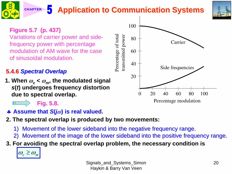
Signals_and_Systems_Simon Haykin amp Barry Van Veen
20
Application to Communication SystemsApplication to Communication SystemsCHAPTER
Figure 57 (p 437)Figure 57 (p 437)Variations of carrier power and side-frequency power with percentage modulation of AM wave for the case of sinusoidal modulation
546 546 Spectral OverlapSpectral Overlap1 When ωc lt ωm the modulated signal
s(t) undergoes frequency distortiondue to spectral overlap
Fig 58Fig 58clubs Assume that S(jω) is real valued2 The spectral overlap is produced by two movements
1)1) Movement of the lower sideband into the negative frequency rangeMovement of the lower sideband into the negative frequency range2)2) Movement of the image of the lower sideband into the positive frMovement of the image of the lower sideband into the positive frequency rangeequency range
3 For avoiding the spectral overlap problem the necessary condition is
c mω ωge
Signals_and_Systems_Simon Haykin amp Barry Van Veen
21
Application to Communication SystemsApplication to Communication SystemsCHAPTER
Figure 58 (p 438)Figure 58 (p 438)Spectral overlap phenomenon in amplitude modulation The phenomenon arises when the carrier frequency ωc is less than the highest frequency component ωm of the modulating signal
v equiv ω p equiv π
547 547 Demodulation of AM WaveDemodulation of AM Wave1 The envelope detector provides a simple yet effective device for the
demodulation of a narrowband AM signal for which the percentage modulation is less than 100
clubsclubs Narrowband means that the carrier is large compared with the mesNarrowband means that the carrier is large compared with the message bandwidthsage bandwidth2 Circuit diagram of an envelope detector Fig 59Fig 59
1) 1) The diode is ideal presenting zero impedance to current flow inThe diode is ideal presenting zero impedance to current flow in the forwardthe forward--biased region and infinite impedance in the reversebiased region and infinite impedance in the reverse--biased region biased region
Signals_and_Systems_Simon Haykin amp Barry Van Veen
22
Application to Communication SystemsApplication to Communication SystemsCHAPTER
Figure 59 (p 438)Figure 59 (p 438)Envelope detector illustrated by (a) circuit diagram (b) AM wave input and (c) envelope detector output assuming ideal conditions
Signals_and_Systems_Simon Haykin amp Barry Van Veen
23
Application to Communication SystemsApplication to Communication SystemsCHAPTER
2) 2) The AM signal applied to the envelope is supplied by a voltage sThe AM signal applied to the envelope is supplied by a voltage source of ource of internal resistance internal resistance RRss
3) The load resistance 3) The load resistance RRll is large compared with the source resistance is large compared with the source resistance RRss During Duringthe charging process the time constant is effectively equathe charging process the time constant is effectively equal to l to RRssCC This time This time constant must be short compared with the carrier period 2constant must be short compared with the carrier period 2ππωωcc that is that is
2s
c
R πω
ltlt (515)
3 The discharging time constant is equal to RlCRRllCC must be large such that the capacitor discharges slowly but notmust be large such that the capacitor discharges slowly but not so so large that the capacitor voltage will not discharge at the maximlarge that the capacitor voltage will not discharge at the maximum rate um rate of change of the modulating wave ieof change of the modulating wave ie2 2
lc m
R Cπ πω ω
ltlt ltlt (516) ωm equiv message
bandwidth
clubs Output ripple can be removed by low-pass filter
Signals_and_Systems_Simon Haykin amp Barry Van Veen
24
Application to Communication SystemsApplication to Communication SystemsCHAPTER
55 55 Double SidebandDouble Sideband--Suppressed ModulationSuppressed Modulation1 In full AM carrier wave c(t) is completely independent of the message signal
m(t)
Transmission of carrier wave A waste of power
2 To overcome this shortcoming we may suppress the carrier component from the modulated wave resulting in double sideband-suppressed carrier(DSB-SC) modulation
3 DSB-SC modulated signal( ) ( ) ( ) cos( ) ( )c cs t c t m t A t m tω= = (517)
clubs This modulated signal undergoes a phase reversal whenever the messagesignal m(t) crosses zero as illustrated in Fig 510Fig 510(a)(a) Message signal Message signal (b)(b) DSBDSB--SC modulated wave resulting from multiplication of the message SC modulated wave resulting from multiplication of the message
signal by the sinusoidal carrier wave signal by the sinusoidal carrier wave
Signals_and_Systems_Simon Haykin amp Barry Van Veen
25
Application to Communication SystemsApplication to Communication SystemsCHAPTER
Figure 510 (p 440)Figure 510 (p 440)Double-sideband-suppressed carrier modulation (a) Message signal (b) DSB-SC modulated wave resulting from multiplication of the message signal by the sinusoidal carrier wave
551 551 FrequencyFrequency--Domain DescriptionDomain Description1 Fourier transform of modulated signal s(t)
1( ) [ ( ( )) ( ( ))]2 c c cS j A M j M jω ω ω ω ω= minus + + (518)
where M(jω) equiv Fourier transform of m(t) minus ωm le ω le ωmFig 511 (a) and (b)Fig 511 (a) and (b)
Signals_and_Systems_Simon Haykin amp Barry Van Veen
26
Application to Communication SystemsApplication to Communication SystemsCHAPTER
Figure 511 (p 441)Figure 511 (p 441)Spectral content of DSB-SC modulated wave (a) Magnitude spectrum of message signal (b) Magnitude spectrum of DSB-SC modulated wave consisting of upper and lower sidebands only
v equiv ω p equiv π
clubs The modulation process simply translates the spectrum of the message signal by plusmn ωc
clubs Transmission bandwidth = 2 ωm2 A device for achieving DSB-SC is called a product modulator or simply
multiplierFig 512 (a)Fig 512 (a) shows the block diagram of a product modulator
Signals_and_Systems_Simon Haykin amp Barry Van Veen
27
Application to Communication SystemsApplication to Communication SystemsCHAPTER
Figure 512 (p 441)Figure 512 (p 441)(a) Product modulator for generating the DSB-SC modulated wave (b) Coherent detector for demodulation of the DSB-SC modulated wave
v equiv ω p equiv π
552 552 Coherent DetectionCoherent Detection1 The message signal m(t) may be recovered from DSB-SC
Fig 512 (b)Fig 512 (b)ss((tt) ) timestimes locally generated sinusoidal wave = locally generated sinusoidal wave = vv((tt))vv((tt) filtered by a Low) filtered by a Low--pass filterpass filter
Local oscillator
2 The local oscillator should be exactly coherent or synchronized in both frequency and phase with the carrier wave c(t)
Signals_and_Systems_Simon Haykin amp Barry Van Veen
28
Application to Communication SystemsApplication to Communication SystemsCHAPTER
Coherent detection or synchronization demodulation3 Derivation for coherent detection
1) Local oscillator cos(ωct + φ )2) Product modulator output
( ) cos( ) ( )cos( ) cos( ) ( )
1 1cos( ) ( ) cos(2 ) ( )2 2
c
c c c
c c c
v t t s tA t t m t
A m t A t m t
ω φω ω φ
φ ω φ
= += +
= + +(519)
1 cos( ) ( )2 cA m tφ
1 cos(2 ) ( )2 c cA t m tω φ+
A scaled version of the original message signal m(t)
DSBDSB--SC modulated signal with carrier SC modulated signal with carrier frequency 2 frequency 2 ωωcc
3) Magnitude spectrum Fig 5134) To clear separate two component of v(t) the original carrier frequency ωc
must satisfy the condition
Signals_and_Systems_Simon Haykin amp Barry Van Veen
29
Application to Communication SystemsApplication to Communication SystemsCHAPTER
Figure 513 (p 442)Figure 513 (p 442)Magnitude spectrum of the product modulator output v(t) in the coherent detector of Fig 512(b)
v equiv ω p equiv π
2 c m mω ω ωminus gt c mω ωgt (520) ωωmm equivequiv message bandwidthmessage bandwidth
4 Specification of low-pass filter1) 1) The cutoff frequency must be The cutoff frequency must be ωωm m 2) The transition band must be 2) The transition band must be ωωm m ≦≦ ωω ≦≦ ωωc c ωωm m
Thus the overall output in Thus the overall output in Fig 512(b)Fig 512(b) is given byis given by1( ) cos( ) ( )2o cv t A m tφ= (521)
cosφ equiv attenuation factor
Signals_and_Systems_Simon Haykin amp Barry Van Veen
30
Application to Communication SystemsApplication to Communication SystemsCHAPTER
5 (1) Demodulated signal vo(t) is proportional to m(t) when the error phase φis a constant
(2) Demodulated signal is maximum when φ = 0 and has a minimum zero when φ = plusmn π2
Example 53 Sinusoidal DSB-SC ModulationConsider again the sinusoidal modulating signal
0 0( ) cos( )m t A tω=
( ) cos( )c cc t A tω=with amplitude A0 and frequency ω0 see Fig 514(a) The carrier wave is
with amplitude Ac and frequency ωc see Fig 514(b) Investigate the time-domain and frequency-domain characteristics of the corresponding DSB-SC modulated waveltltSolgtSolgt
clubs φ = plusmn π2 represents the quadrature null effect of the coherent detector
1 The modulated DSB-SC signal is defined by
0 0
0 0 0 0
( ) cos( ) cos( )1 1cos[( ) ] cos[( ) ]2 2
c c
c c c c
s t A A t t
A A t A A t
ω ω
ω ω ω ω
=
= + + minus
Signals_and_Systems_Simon Haykin amp Barry Van Veen
31
Application to Communication SystemsApplication to Communication SystemsCHAPTER
2 The Fourier transform of s(t) is given by
0 0 0
0 0
1( ) cos[ ( ) ( )]2
( ) ( )
c c c
c c
S j A Aω π δ ω ω ω δ ω ω ω
δ ω ω ω δ ω ω ω
= minus minus + + +
+ minus + + + minus
which consists of four weighted impulse functions at the frequencies ωc+ ω0-ωc- ω0 ωc- ω0 and- ωc+ ω0 as illustrated in the right-hand side of Fig Fig 514(c)514(c)
3 This Fourier transform differs from that depicted in the right-hand side of Fig Fig 56(c)56(c) for the corresponding example of full AM in one important respect The impulse functions at plusmn ωc due to the carrier are removed
4 Application of the sinusoidally modulated DSB-SC signal to the product modulator of Fig 512(b) yields the output (assuming φ = 0)
0 0 0
0 0 0 0 0
1( ) cos( ) cos[( ) ] cos[( ) ]21 cos[(2 ) ] cos( ) cos[(2 ) ] cos( )4
c c c c
c c c
v t A A t t t
A A t t t t
ω ω ω ω ω
ω ω ω ω ω ω
= + + minus
= + + + minus +
Signals_and_Systems_Simon Haykin amp Barry Van Veen
32
Application to Communication SystemsApplication to Communication SystemsCHAPTER
Figure 514 (p Figure 514 (p 443)443)Time-domain (on the left) and frequency-domain (on the right) characteristics of DSB-SC modulation produced by a sinusoidal modulating wave (a) Modulating wave (b) Carrier wave (c) DSB-SC modulated wave Note that ω= 2πƒ
v equiv ω p equiv π
Signals_and_Systems_Simon Haykin amp Barry Van Veen
33
Application to Communication SystemsApplication to Communication SystemsCHAPTER
5 The first two sinusoidal terms of v(t) are produced by the upper side frequency and the last two sinusoidal terms are produced by the lower side frequency
6 With ωcgt ω0 the first and third sinusoidal terms of frequencies 2ωc+ ω0 and 2ωc-ω0 respectively are removed by the low-pass filter of Fig 512(b)Fig 512(b) which leaves the second and fourth sinusoidal terms of frequency ω0 as the only output of the filter The coherent detector output thus reproduces the original modulating wave
7 Note however that this output appears as two equal terms one derived from the upper side frequency and the other from the lower side frequency We therefore conclude that for the transmission of the sinusoidal signal A0 cos(ω0t) only one side frequency is necessary (The issue will be discussed further in Section 57Section 57)
553 553 CostasCostas ReceiverReceiver1 Costas receiver Fig 515Fig 5152 This receiver consists of two coherent detector supplied with the same input
ie the incoming DSB-Sc wave
cos(2 ) ( )c cA f t m tπ but with individual local oscillator signals that are in phase duadrature with respect to each other
In-phase coherent detector (I-Channel) and quadrature-phase coherent detector (Q-Channel)
Signals_and_Systems_Simon Haykin amp Barry Van Veen
34
Application to Communication SystemsApplication to Communication SystemsCHAPTER
Figure 515 (p 445)Figure 515 (p 445)Costas receiver
v equiv ω p equiv π
Signals_and_Systems_Simon Haykin amp Barry Van Veen
35
Application to Communication SystemsApplication to Communication SystemsCHAPTER
56 56 QuadratureQuadrature--Carrier MultiplexingCarrier Multiplexing
Figure 516 (p 446)Figure 516 (p 446)Quadrature-carrier multiplexing system exploiting the quadrature null effect (a) Transmitter (b) Receiver assuming perfect synchronization with the transmitter
v equiv ω p equiv π
1 1 A A quadraturequadrature--carrier multiplexing or carrier multiplexing or quadraturequadrature--amplitude modulation (QAM) amplitude modulation (QAM) system enables two DSBsystem enables two DSB--SC modulated waves to occupy the same transmission SC modulated waves to occupy the same transmission bandwidth and yet it allows for their separation at the receivebandwidth and yet it allows for their separation at the receiver outputr output
BandwidthBandwidth--conservation schemeconservation scheme
Signals_and_Systems_Simon Haykin amp Barry Van Veen
36
Application to Communication SystemsApplication to Communication SystemsCHAPTER
2 Fig 5-16(a) Block diagram of the quadrature-carrier multiplexing systemFig 5-16(a) transmitter Fig 5-16(b) receiver
3 Multiplexed signal s(t)
(522) 1 2( ) ( ) cos( ) ( )sin( )c c c cs t A m t t A m t tω ω= +
where m1(t) and m2(t) denotes the two different message signals applied to the product modulations
clubsTransmission bandwidth = 2 ωm centered at ωc where ωm is the commonmessage bandwidth of m1(t) and m2(t)
4 The output of the top detector at receiver is 1
12 ( )cA m t
The output of the bottom detector at receiver is1
22 ( )cA m t
57 57 Other Variants of Amplitude Modulation Other Variants of Amplitude Modulation clubs Basic concept Full AM and DSB-SC rArr Wasteful of bandwidthclubs Given the amplitude and phase spectra of either lower or upper sideband
we can uniquely determine the other
Signals_and_Systems_Simon Haykin amp Barry Van Veen
37
Application to Communication SystemsApplication to Communication SystemsCHAPTER
clubs Single-sideband (SSB) modulation only one sideband is transmitted571 571 FrequencyFrequency--Domain Description of SSB ModulationDomain Description of SSB Modulation1 Consider a message signal m(t) with a spectrum M(jω) limited to the band
ωa le ω le ωb Fig 5-17 (a)2 DSB-SC modulated signal
( ) cos( )c cm t A tωtimes Fig 5-17 (b)
3 (1) Upper sideband the frequencies above ωc and below minus ωc(2) Upper sideband the frequencies below ωc and above minus ωc
Fig 5-17 (c)4 When only the lower sideband is transmitted the spectrum of the
corresponding SSB modulated wave is as shown in Fig 5-17 (d) 5 Advantages of SSB
(1) Reduced bandwidth requirement(2) Elimination of the high-power carrier waveDisadvantage od SSB(1) Cost and complexity of implementing both the transmitter and receiver
Signals_and_Systems_Simon Haykin amp Barry Van Veen
38
Application to Communication SystemsApplication to Communication SystemsCHAPTER
Figure 517 Figure 517 (p 447)(p 447)Frequency-domain characteristics of SSB modulation (a) Magnitude spectrum of message signal with energy gap from ndash ωa to ωa
(c) Magnitude spectrum of SSB modulated wave containing upper sideband only
(d) Magnitude spectrum of SSB modulated wave containing lower sideband only
(b) Magnitude spectrum of DSB-SC signal
v equiv ω p equiv π
Signals_and_Systems_Simon Haykin amp Barry Van Veen
39
Application to Communication SystemsApplication to Communication SystemsCHAPTER
6 Frequency-discrimination scheme for producing SSB modulation Fig 518clubs Bandpass filter is designed to pass the sideband selected for transmission
and suppress the remaining sidebandclubs Requirement in SSB signal the message signal applied to the product
modulator must have a energy gap in its spectrum Refer to Fig 517 (a)
Figure 518 (p 448)Figure 518 (p 448)System consisting of product modulator and bandpass filter for generating SSB modulated wave
v equiv ω p equiv π
572 572 TimeTime--Domain Description of SSB ModulationDomain Description of SSB Modulation1 Mathematical tool Hilbert transform
The Hilbert transform of a signal x(t) is defined by1 ( ) 1ˆ( ) ( )xx t d x t
t tτ τ
π τ πinfin
minusinfin= = lowast
minusint
Signals_and_Systems_Simon Haykin amp Barry Van Veen
40
Application to Communication SystemsApplication to Communication SystemsCHAPTER
The Fourier transform of 1(πt) is minus j times the signum function denoted
1 for 0sgn( ) 0 for 0
1 for 0
ωω ω
ω
+ gt⎧⎪= =⎨⎪minus lt⎩
2 Passing x(t) through a Hilbert transformer is equivalent to the combination of the following two operations in frequency domain1) Keeping X(jω)unchanged for all ω 2) Shifting areX(jω) (ie the phase spectrum of x(t)) by +90deg for negative
frequencies and minus 90deg for positive frequencies clubs Hilbert transformer = Wideband minus 90deg phase shifter 573 573 Vestigial Sideband ModulationVestigial Sideband Modulation1 When the message signal contains significant components at extremely
low frequencies the upper and lower sidebands meet at the carrier frequency
Using SSB is inappropriateUsing SSB is inappropriateEx TV signals or
wideband dataUsing VSB (Vestigial sideband) modulation is appropriateUsing VSB (Vestigial sideband) modulation is appropriate
Signals_and_Systems_Simon Haykin amp Barry Van Veen
41
Application to Communication SystemsApplication to Communication SystemsCHAPTER
2 VSB is a compromise between SSB and DSB-SC forms of modulationIn VSB modulation one sideband is passes almost completely whereas just a trace or vestige of the other sideband is retained
3 Fig 519 illustrates a VSB modulated wave s(t) in relation to the message signal m(t)
v equiv ω p equiv π
Figure 519 (p 449)Figure 519 (p 449)Spectral content of VSB modulated wave (a) Magnitude spectrum of message signal (c) Magnitude spectrum of VSB modulated wave containing a vestige of the lower sideband
clubs The lower sideband is modified into the vestigial sideband4 Transmission bandwidth of VSB modulated wave T m vω ω ω= + (523)
where ωm is the message bandwidth and ωu is the width of the vestigial sideband
Signals_and_Systems_Simon Haykin amp Barry Van Veen
42
Application to Communication SystemsApplication to Communication SystemsCHAPTER
5 Generation of VSB modulated wave Fig 520
Figure 520 (p 450)Figure 520 (p 450)System consisting of product modulator and sideband shaping filter for generating VSB modulated wave
v equiv ω p equiv π
Passing a DSBPassing a DSB--SC modulated wave through a sidebandSC modulated wave through a sideband--shaping filtershaping filter6 The sideband-shaping filter is designed so that the original message
spectrum M(jω) is reproduced on the demodulation as a result of the superposition of two spectra
1) The positive-frequency part of S(jω) (ie the Fourier transform of the transmitted signal s(t)) shifted downward in frequency by ωc
2) The negative-frequency part of S(jω) shifted upward in frequency by ωc
Fig 521 A reflection of the vestige of the lower sideband makes up for the missing parts of the upper sideband
Signals_and_Systems_Simon Haykin amp Barry Van Veen
43
Application to Communication SystemsApplication to Communication SystemsCHAPTER
Figure 521 (p 450)Figure 521 (p 450)Superposition of the two spectra shown in parts (a) and (b) of the figure results in the original message spectrum (shown dashed) upon demodulation
58 58 PulsePulse--Amplitude Modulation Amplitude Modulation clubs Basic concept
Basic role in the operation of AM Frequency-shiftingBasic role in the operation of PAM Sampling
581 581 Sampling RevisitedSampling Revisited1 Sampling theorem
In view point of PAMIn view point of PAM
Signals_and_Systems_Simon Haykin amp Barry Van Veen
44
Application to Communication SystemsApplication to Communication SystemsCHAPTER
1) A band-limited signal of finite energy that has no radian frequency components higher than ωm is uniquely determined by the values of the signal at instants of time separated by π ωm seconds
2) A band-limited signal of finite energy that has no radian frequency components higher than ωm may be completely recovered from a knowledge of its samples taken at the rate of ωm π per seconds
clubs Part 1) rArr Be exploited in the transmitter of a PAM clubs Part 2) rArr Be exploited in the Receiver of a PAM2 To combat the effects of aliasing in practice we use two corrective measures1) Prior to sampling a low-pass antialiasing filter is used to attenuate those high-
frequency components of the signal which lie outside the band of interest2) The filtered signal is sampled at a rate slightly higher than the Nyquist rate3 Generation of a PAM signal Fig 522Fig 522Example 54 Telephonic CommunicationThe highest frequency component of a speech signal needed for telephonic communication is about 31 kHz Suggest a suitable value for the sampling rate ltltSolgtSolgt
Signals_and_Systems_Simon Haykin amp Barry Van Veen
45
Application to Communication SystemsApplication to Communication SystemsCHAPTER
Figure 522 (p 451)Figure 522 (p 451)System consisting of antialiasing filter and sample-and-hold circuit for converting a message signal into a flattopped PAM signal
1 The highest frequency component of 31 kHz corresponds to 362 10 radsmω π= times
Correspondingly the Nyquist rate is
62 kHzmωπ
=
2 A suitable value for the sampling rate-one slightly higher than the Nyquistrate-may be 8 kHz a rate that is the international standard for telephone speech signals
Signals_and_Systems_Simon Haykin amp Barry Van Veen
46
Application to Communication SystemsApplication to Communication SystemsCHAPTER
582 582 Mathematical Description of PAMMathematical Description of PAM1 The carrier wave used in PAM consists of a sequence of short pulses of
fixed duration in terms of which PAM is formally defined as followsPAM is a form of pulse modulation in which the amplitude of the PAM is a form of pulse modulation in which the amplitude of the pulsed carrier is pulsed carrier is varied in accordance with instantaneous sample values of the mesvaried in accordance with instantaneous sample values of the message signalsage signal the duration of the pulsed carrier is maintained constant throughout
Fig 523Fig 523
Figure 523 (p452) Figure 523 (p452) Waveform of flattopped PAM signal with pulse duration T0 and sampling period Ts
Signals_and_Systems_Simon Haykin amp Barry Van Veen
47
Application to Communication SystemsApplication to Communication SystemsCHAPTER
2 Mathematical representation of the PAM
( ) [ ] ( )sn
s t m n b t nTinfin
=minusinfin
= minussum (524) s(t) equiv PAM signal m(t) equiv
message signal
Ts equiv sampling period m[n] equiv the values of m(t) at t = nTs h(t) equiv rectangular pulse of the unit amplitude and duration T0
3 Rectangular pulse
01 0( )
0 otherwiset T
h tlt lt⎧
= ⎨⎩
(525) Fig 524 (a)Fig 524 (a)
clubs Eq (524) is a sample-and-hold operationAnalogous to zeroAnalogous to zero--orderorder--holdhold--
based reconstruction in Sec 46based reconstruction in Sec 46
差異差異hh((tt) ) 的的TTss與與TT00
4 Impulse-sampled version of message signal m(t)
( ) [ ] ( )sn
m t m n t nTδ δinfin
=minusinfin
= minussum (526)
5 PAM signal( ) [ ] ( )
( ) ( )
sn
s t m n b t nT
m t b tδ
infin
=minusinfin
= minus
=
sum(527)
Convolution of impulse-sampled version mδ(t) and h(t)
Time domain Time domain operationoperation
Signals_and_Systems_Simon Haykin amp Barry Van Veen
48
Application to Communication SystemsApplication to Communication SystemsCHAPTER
Figure 524 (p 453)(a) Rectangular pulse h(t) of unit amplitude and duration T0 (b) Magnitude spectrum |H(jω)| and phase spectrum argH(jω) of pulse h(t)
v equiv ω p equiv π
Signals_and_Systems_Simon Haykin amp Barry Van Veen
49
Application to Communication SystemsApplication to Communication SystemsCHAPTER
6 FT of PAM signal( ) ( ) ( )S j M j H jδω ω ω= (528)
where( ) ( )FTS j s tω larr⎯rarr ( ) ( )FTM j m tδ δω larr⎯rarr ( ) ( )FTH j h tω larr⎯rarr
7 Impulse sampling of the message signal m(t) introduces periodicity into the spectrum as given by
1( ) ( ( ))sks
M j M j kTδ ω ω ω
infin
=minusinfin
= minussum (529) 1Ts equiv sampling rate ωs = 2πTs rads
1( ) ( ( )) ( )sks
S j M j k H jT
ω ω ω ωinfin
=minusinfin
= minussum (530)
( ) ( )FTM j m tω larr⎯rarrwhere
clubs Suppose that m(t) is strictly band limited and that the sampling rate 1Ts is greater than the Nyquist rate Then passing s(t) through a reconstruction filter chosen as an ideal low-pass filter with cutoff frequency ωm and gain Ts we find that the spectrum of the resulting filter output is equal to M(jω)H(jω)
Signals_and_Systems_Simon Haykin amp Barry Van Veen
50
Application to Communication SystemsApplication to Communication SystemsCHAPTER
8 From Eq (525) we find that0 2
0 0( ) sin ( (2 )) j TH j T c T e ωω ω π minus= (531) Fig 524(b) magnitude and phase of H(jω)
clubs Using PAM to represent a continuous-time message signal we introduce amplitude distortion as well as a delay of T02
clubs The frequency distortion caused by the use of flat-topped sampled in the generation of a PAM wave illustrated in Fig 523Fig 523 is referred to as the aperture effect
583 583 Demodulation of PAM SignalDemodulation of PAM Signal1 Reconstruction scheme Fig 525Fig 525
Figure 525 (p 454)Figure 525 (p 454)System consisting of low-pass interpolation filter and equalizer for reconstructing a message signal from its flattopped sampled version
clubs The system consists of low-pass interpolation filter and equalizer connected in cascade
Signals_and_Systems_Simon Haykin amp Barry Van Veen
51
Application to Communication SystemsApplication to Communication SystemsCHAPTER
2 The cutoff frequency of low-pass filter = the highest frequency ωm of message signal
3 The equalizer is used to correct the aperture effect due to flat-topped sampling in the sample-and-hold circuit
4 The equalizer has the effect of decreasing the in-band loss of the interpolation filter as frequency increases in such a manner as to compensate for the aperture effect
5 Amplitude response of equalizer
0
0 0 0 0
1 1 1| ( ) | | sinc( 2) | 2 | sin( 2) |
TH j T T T T
ωω ω ω
= =
Frequency response Eq (531)
Example 55 Equalization for PAM TransmissionThe duty cycle in a PAM signal namely T0 Ts is 10 Evaluate the peak amplification required for equalizationltltSolgtSolgt1 At ωm = π Ts which corresponds to the highest frequency component of the
message signal for a sampling rate equal to the Nyquist rate we find from Eq (531) that the magnitude response of the equalizer at ωm normalized to that at zero frequency is
Signals_and_Systems_Simon Haykin amp Barry Van Veen
52
Application to Communication SystemsApplication to Communication SystemsCHAPTER
Figure 526 (p 455)Figure 526 (p 455)Normalized equalization (to compensate for aperture effect) plotted against the duty cycle T0Ts
Signals_and_Systems_Simon Haykin amp Barry Van Veen
53
Application to Communication SystemsApplication to Communication SystemsCHAPTER
0
0 0
( 2)( )1sin (05 ) sin[( 2)( )]
s
s s
T Tc T T T T
ππ
=
where the ratio T0 Ts is equal to the duty cycle of the sampling pulses 2 In Fig 526Fig 526 this result is plotted as a function of the duty cycle T0 Ts Ideally it
should be equal to unity for all values of T0 Ts 3 For a duty cycle of 10 it is equal to 10041 It follows that for duty cycles of less
than 10 the magnitude equalization required is less than 10041 in which case the aperture effect is usually considered to be negligible
59 59 Multiplexing Multiplexing clubs Three basic types of multiplexing1 Frequency-division multiplexing in which the signals are separated by
allocating them to different frequency bands This is illustrated in Fig 527(a) for the case of six different message signals Frequency-division multiplexing favors the use of CW modulation where each message signal is able to use the channel on a continuous-time basis
2 Time-division multiplexing wherein the signals are separated by allocating them to different time slots within a sampling interval
Signals_and_Systems_Simon Haykin amp Barry Van Veen
54
Application to Communication SystemsApplication to Communication SystemsCHAPTER
This second type of multiplexing is illustrated in Fig 527(b) for the case of six different message signals Code-division multiplexing which relies on the assignment of different codes to the individual users of the channel
3 Code-division multiplexing which relies on the assignment of different codes to the individual users of the channel
591 591 FrequencyFrequency--Domain Multiplexing (FDM)Domain Multiplexing (FDM)1 Block diagram Fig 528Fig 5282 Incoming message signals low-pass variety3 Low-pass filter to remove high-frequency components such that the signal
in each channel does not disturb each other4 MOD (modulator) shift the frequency ranges of the signals so as to occupy
mutually exclusive frequency intervalsSSB is often used in this stageEx Voice input is usually assigned a bandwidth of 4 kHz
5 Band-pass filters are used to restrict the band of each modulated wave to its prescribed range
6 Band-pass filters in receiver separate the message signals7 DEM (demodulator) to recover signalsclubs FDM in Fig 528 operates in only one direction
Signals_and_Systems_Simon Haykin amp Barry Van Veen
55
Application to Communication SystemsApplication to Communication SystemsCHAPTER
Figure 527 (p 456)Figure 527 (p 456)Two basic forms of multiplexing (a) Frequency-division multiplexing (with guardbands) (b) Time-division multiplexing no provision is made here for synchronizing pulses
Signals_and_Systems_Simon Haykin amp Barry Van Veen
56
Application to Communication SystemsApplication to Communication SystemsCHAPTER
Figure 528 (p 457)Figure 528 (p 457)Block diagram of FDM system showing the important constituents of the transmitter and receiver
Signals_and_Systems_Simon Haykin amp Barry Van Veen
57
Application to Communication SystemsApplication to Communication SystemsCHAPTER
Example 56 SSB-FDM System
ltltSolgtSolgt
An FDM system is used to multiplex 24 independent voice signals SSB modulation is used for the transmission Given that each voice signal is allotted a bandwidth 4kHz calculate the overall transmission bandwidth of the channel
With each voice signal allotted a bandwidth of 4 kHz the use of SSB modulation requires a bandwidth of 4 kHz for its transmission Accordingly the overall transmission bandwidth provided by the channel is 24 X 4 = 96 kHz 592 592 TimeTime--Domain Multiplexing (TDM)Domain Multiplexing (TDM)clubs Basic to the operation of a TDM system is the sampling theoremclubs The transmission of the message samples engages the transmission channel for
only a fraction of the sampling interval on a periodic basis equal to the width T0 of a PAM modulating pulse
1 Block diagram Fig 529Fig 5292 Commutator is usually implemented by means of electronic switching
circuitry3 The function of commutator is two folds
Signals_and_Systems_Simon Haykin amp Barry Van Veen
58
Application to Communication SystemsApplication to Communication SystemsCHAPTER
Figure 529 (p 458)Figure 529 (p 458)Block diagram of TDM system showing the important constituents of the transmitter and receiver
(1) To take a narrow sample of each of the M input message signals at a rate 1Tsthat is slightly higher than ωcπ where ωc is the cutoff frequency of the input low-pass filter
(2) To sequentially interleave these M samples inside a sampling interval Ts4 Pulse modulator transform the multiplexed signal into a form suitable for
transmission over the common channel
Signals_and_Systems_Simon Haykin amp Barry Van Veen
59
Application to Communication SystemsApplication to Communication SystemsCHAPTER
clubs The use of time-division multiplexing introduces a bandwidth expansion factor M because the scheme must squeeze M samples derived from M independent message sources into a time slot equal to one sampling interval
5 Pulse demodulator performs the inverse operation of the pulse modulator6 Decommutator distributes the narrow samples produced by pulse demodulator to the appropriate low-pass reconstruction filter7 Synchronization between the timing operations of the transmitter and
receiver in a TDM system is essential for satisfactory performance of the system
Inserting an extra pulse into each sampling interval on a regular basisBandwidth expansion factor is increased to M + 1
clubs The TDM system is hghly sensitive to the dispersion in the common transmission channel
Example 57 Comparison of TDM with FDMATDM system is used to multiplex four independent voice signals using PAM Each voice signal is sampled at the rate of 8 kHz The system incorporates a synchronizing pulse train for its proper operation
Signals_and_Systems_Simon Haykin amp Barry Van Veen
60
Application to Communication SystemsApplication to Communication SystemsCHAPTER
(a) Determine the timing relationships between the synchronizing pulse train and the impulse trains used to sample the four voice signals
(b) Calculate the transmission bandwidth of the channel for the TDM system and compare the result with a corresponding FDM system using SSBmodulation
ltltSolgtSolgt(a) The sampling period is
31 125 s
8 10sT s μ= =times
In this example the number of voice signals is M = 4 Hence dividing the sampling period of 125 μs among these voice signals and the synchronizing pulse train we obtain the time slot allocated to each one of them
0 1125 25 s
5
sTTM
μ
=+
= =
Signals_and_Systems_Simon Haykin amp Barry Van Veen
61
Application to Communication SystemsApplication to Communication SystemsCHAPTER
Figure 530Figure 530 shows the timing relationships between the synchronizing pulse train and the four impulse trains used to sample the different voice signals in a single frame Each frame includes time slots of common duration T0 = 25 μs which are allocated to the pulse-modulated signals and synchronizing pulse
Figure 530 (p 459)Figure 530 (p 459)Composition of one frame of a multiplexed PAM signal incorporating four voice-signals and a synchronizing pulse
Signals_and_Systems_Simon Haykin amp Barry Van Veen
62
Application to Communication SystemsApplication to Communication SystemsCHAPTER
(b) As a consequence of the time-bandwidth product (see Section 317) there is an inverse relationship between the duration of a pulse and the bandwidth (ie cutoff frequency) of the channel needed for itstransmission Accordingly the overall transmission bandwidth of the channel is
0
21 1 MHz 40 kHz
25
TTf
T
ωπ
=
= = =
In contrast the use of an FDM system based on SSB modulation requires a channel bandwidth equal to M times that of a single voice signal-that is 4 X 4 = 16 kHz Thus the use of PAM-TDM requires a channel bandwidth that is 40 16 = 25 times that of SSB-FDMIn practice pulse-code modulation is commonly used as the method of modulation for TDM this results in a further increase in channel bandwidth depending on the length of the code word used in the digital representation of each pulse in the PAM signal
Signals_and_Systems_Simon Haykin amp Barry Van Veen
63
Application to Communication SystemsApplication to Communication SystemsCHAPTER
510 510 Pulse and Group Delays Pulse and Group Delays 1 Whenever a signal is transmitted through a dispersive (ie frequency
selective) system some delay is introduced into the output signal in relation to the input signal
2 The delay is determined by the phase response of the system3 Phase response of a dispersive communication channel
( ) arg ( )H jφ ω ω= (532)
A signal is transmitted through the channel at a frequency ωc The signal received at the channel lags the transmitted signal by φ(ωc) The time delay is called phase delay formally defined as
( )cp
c
φ ωτω
= minus (533)
The phase delay is not necessarily the true signal delayclubs Case study for DSB-SC1 Transmitted signal
0( ) cos( ) cos( )cs t A t tω ω= (534)
ωc equiv carrier frequency ω0 equiv sinusoidal modulation frequency
A = AcA0
Signals_and_Systems_Simon Haykin amp Barry Van Veen
64
Application to Communication SystemsApplication to Communication SystemsCHAPTER
1 21 1( ) cos( ) cos( )2 2
s t A t A tω ω= +
1 0cω ω ω= + (535) where
2 0cω ω ω= minus (536)
Upper frequency
Lower frequency
2 Let the s(t) be transmitted through the channel with phase response φ (ω) Accordingly the signal received at the channel output is
1 1 2 21 1( ) cos( ( )) cos( ( ))2 2
y t A t A tω φ ω ω φ ω= + + +
1 2 1 20
( ) ( ) ( )1 ( )( ) cos cos2 2cy t A t tφ ω φ ω φ ω φ ωω ω+⎛ ⎞ ⎛ ⎞= + +⎜ ⎟ ⎜ ⎟
⎝ ⎠ ⎝ ⎠(537)
3 Two observations from Eq (537)1) The carrier component at frequency ωc in y(t) lags its counterpart in s(t) by
frac12 (φ (ω1) + φ (ω2)) which represents a time delay equal to
1 2 1 2
c 1 2
( )+ ( ) ( )+ ( )2 +
φ ω φ ω φ ω φ ωω ω ω
minus = minus (538)
Signals_and_Systems_Simon Haykin amp Barry Van Veen
65
Application to Communication SystemsApplication to Communication SystemsCHAPTER
2) The message component at frequency ω0 in y(t) lags its counterpart in s(t) by frac12 (φ (ω1) minus φ (ω2)) which represents a time delay equal to
1 2 1 2
0 1 2
( ) ( ) ( ) ( )2
φ ω φ ω φ ω φ ωω ω ωminus minus
minus = minusminus
(539)
4 Suppose that ω0 lt ωc rArr the side frequencies are close together with ω c between them Such a modulated signal is said to be a narrowband signal The phase response φ (ω) in the vicinity of ω = ωc is approximated by two-term Taylor series expansion
( )( ) ( ) ( )c
c cd
d ω ω
φ ωφ ω φ ω ω ωω =
= + times minus (540)
Phase delay = ( ) c cφ ω ωminus
5 The time delay introduced by the message signal (ie he ldquoenveloperdquo of the modulated signal) is given by
( )
c
gd
d ω ω
φ ωτω =
= minus (541) The time delay τg is called the
envelope delay or group delay
Signals_and_Systems_Simon Haykin amp Barry Van Veen
66
Application to Communication SystemsApplication to Communication SystemsCHAPTER
6 When a modulated signal is transmitted through a communication channel there are two different delays to be considered1) The carrier or phase delay τp defined by Eq (533)2) The envelope or group delay τg defined by Eq (541)
clubs The group delay is the true signal delay
Example 58 Phase and Group Delays for Ban-pass Channel
ltltSolgtSolgt
The phase response of a band-pass communication channel is defined by 2 2
1( ) tan c
c
ω ωφ ωωω
minus ⎛ ⎞minus= minus ⎜ ⎟
⎝ ⎠The signal s(t) defined in Eq (534) is transmitted through this channel with
475 radscω = 0 025 radsω =andCalculate (a) the phase delay and (b) the group delay
(a) At ω = ωc φ (ωc) = 0 According to Eq (533) the phase delay τ p is zero (b) Differentiating φ (ω) with respect to ω we get
Signals_and_Systems_Simon Haykin amp Barry Van Veen
67
Application to Communication SystemsApplication to Communication SystemsCHAPTER
2 2
2 2 2 2 2
( )( )( )
c c
c c
dd
ω ω ωφ ωω ω ω ω ω
+= minus
+ minus
Using thing result in Eq (541) we find that the group delay is 2 2 04211
475gc
sτω
= = =
1 One waveform shown as a solid curve was obtained by multiplying the transmitted signal s(t) by the carrier wave cos(ωct)
2 The second waveform shown as a dotted curve was obtained by multiplying the received signal y(t) by the carrier wave cos(ωct)
To display the results obtained in parts (a) and (b) in graphical form Fig 531Fig 531shows a superposition of two waveforms obtained as follows
The figure clearly shows that the carrier (phase) delay τ p is zero and the envelope of the received signal y(t) is lagging behind that of the transmitted signal by τs seconds For the presentation of waveforms in this figure we purposely did not use a filter to suppress the high frequency components resulting from the multiplications described under points 1 and 2 because of the desire to retain a contribution due to the carrier for display
Signals_and_Systems_Simon Haykin amp Barry Van Veen
68
Application to Communication SystemsApplication to Communication SystemsCHAPTER
Figure 531 Figure 531 (p 463)(p 463)Highlighting the zero carrier delay (solid curve) and group delay τg (dotted curve) which are determined in accordance with Example 58
Signals_and_Systems_Simon Haykin amp Barry Van Veen
69
Application to Communication SystemsApplication to Communication SystemsCHAPTER
clubs Not also that the separation between the upper side frequency ω1 = ωc + ω0 = 500 rads and the lower side frequency ω2 = ωc minus ω0 = 450 rads is about 10 of the carrier frequency ωc = 475 rads which justifies referring to the modulated signal in this example as a narrowband signal
5101 5101 Some Practical ConsiderationsSome Practical Considerationsclubs What is the practical importance of group delay 1 Eq (541) for determining group delay applies strictly to narrowband
modulated signal2 The message bandwidth may be comparable to the carrier frequency In
this situation the group delay is formulated as a frequency-dependent parameter ie ( )d( )g d
φ ωτ ωω
= minus (542)
3 When a wideband modulated signals transmitted through a dispersive channel the frequency components of the message signal are delayed by different amounts at the channel output
Delay distortionFig 532Fig 532 Group delay response of voice-grade telephone channel
Signals_and_Systems_Simon Haykin amp Barry Van Veen
70
Application to Communication SystemsApplication to Communication SystemsCHAPTER
Figure 532 (p 464)Group delay response of voice-grade telephone channel (Adapted from J C Bellamy Digital Telephony Wiley 1982)
511 511 Exploring Concepts with MATLABExploring Concepts with MATLAB5111 5111 Full AMFull AMclubs Sinusoidal modulation
clubs To reconstruct a faithful version of the original message signal in the receiver we have to use a delay equalizer
0( ) [1 cos( )]cos( )c cs t A t tμ ω ω= +1 AM experiment
1cA =
08 radscω π= 0 01 radsω π=Carrier amplitude
Carrier frequency Modulation amplitude
Signals_and_Systems_Simon Haykin amp Barry Van Veen
71
Application to Communication SystemsApplication to Communication SystemsCHAPTER
2 We wish to display and analyze 10 full cycles of the AM wave corresponding to a total duration of 200 s Choosing a sampling rate 1Ts = 10 Hz we have a total of N = 2000 time samples The frequency band of interest is minus 10 π ≦ ω ≦ 10 π Since the separation between the carrier and either side frequency is equal to the modulation frequency ω0 = 01 π rads we would like to have a frequency resolution ωr = 001π rads To achieve this resolution we require the following number of frequency samples (see Eq (442))
20 2000001
s
r
M ω πω π
ge = =
3 We therefore choose M = 2000 To approximate the Fourier transform of the AM wave s(t) we may use a 2000-point DTFS The only variable in the AM experiment is the modulation factor μ with respect to which we wish to investigate three different situationsμ = 05 corresponding to under-modulationμ = 10 for which the AM system is on the verge of over-modulationμ = 20 corresponding to over-modulation
Signals_and_Systems_Simon Haykin amp Barry Van Veen
72
Application to Communication SystemsApplication to Communication SystemsCHAPTER
4 MATLAB commandsAc = 1 carrier amplitudewc = 08pi carrier frequencyw0 = 01pi modulation frequencymu = 05 modulation factort = 0011999s = Ac(1 + mucos(w0t))cos(wct)plot(ts)Smag = abs(fftshift(fft(s2000)))2000 Smag denotes the magnitude specturm of the AM wavew = 10[-1000999]2pi2000plot(wSmag)axis ([-30 30 0 08])
5 5 μμ = 05 = 05 case case Fig 533Fig 533μμ = 10 case = 10 case Fig 534Fig 534μμ = 20 case = 20 case Fig 535Fig 535
Discussion see pp 466-469 textbook
Signals_and_Systems_Simon Haykin amp Barry Van Veen
73
Application to Communication SystemsApplication to Communication SystemsCHAPTER
-30 -20 -10 0 10 20 300
02
04
06
0 50 100 150 200-2
-1
0
1
2
2 22 24 26 28 3
02
04
06
(a) Time (s)
Time domain
Frequency domain
(b) Frequency (rads)
Frequency domain
Frequency (rads)
Figure 533 (p 466)Amplitude modulation with 50 modulation (a) AM wave (b) magnitude spectrum of the AM wave and (c) expanded spectrum around the carrier frequency
μμ = 05 = 05 casecase
Signals_and_Systems_Simon Haykin amp Barry Van Veen
74
Application to Communication SystemsApplication to Communication SystemsCHAPTER
Figure 534 (p 467)Figure 534 (p 467)Amplitude modulation with 100 modulation (a) AM wave (b) magnitude spectrum of the AM wave and (c) expanded spectrum around the carrier frequency
Signals_and_Systems_Simon Haykin amp Barry Van Veen
75
Application to Communication SystemsApplication to Communication SystemsCHAPTER
Figure 535 (p 468)Amplitude modulation with 200 modulation (a) AM wave (b) magnitude spectrum of the AM wave and (c) expanded spectrum around the carrier frequency
Signals_and_Systems_Simon Haykin amp Barry Van Veen
76
Application to Communication SystemsApplication to Communication SystemsCHAPTER
5112 5112 DSBDSB--SC ModulationSC Modulation1 Sinusoidal modulation
0 0( ) cos( ) cos( )c cs t A A t tω ω=
2 MATLAB commands
Ac = 1 carrier amplitudewc = 08pi carrier frequency in radsA0 = 1 amplitude of modulating signalw0 = 01pi frequency of modulating signalt = 011999s = AcA0cos(wct)cos(w0t)plot(ts)Smag = abs(fftshift(fft(s2000)))2000w = 10[-1000999]2pi2000plot(wSmag)
3 3 DSBDSB--SC modulated waveSC modulated wave Fig 536Fig 536 Discussion see pp 466-469 textbook
4 Output of the product modulator in Fig 512 (b) with φ = 0
Signals_and_Systems_Simon Haykin amp Barry Van Veen
77
Application to Communication SystemsApplication to Communication SystemsCHAPTER
Figure 536 (p 469)DSB-SC modulation (a) DSB-SC modulated wave (b) magnitude spectrum of the modulated wave and (c) expanded spectrum around the carrier frequency
Signals_and_Systems_Simon Haykin amp Barry Van Veen
78
Application to Communication SystemsApplication to Communication SystemsCHAPTER
( ) ( ) cos( )cv t s t tω=
5 MATLAB commandsgtgt v = scos(wct)
6 Fig 537 (a) waveforms of v(t) Fig 537 (b) magnitude spectrum which readily shows that v(t) consists of the following components1) A sinusoidal component with frequency 01π rads representing the
modulating wave2) A new DSB-SC modulated wave with double carrier frequency of 16π rads
in actuality the side frequencies of this modulated wave are located at 15πand 17π rads
1) The frequency of the modulating wave lies inside the passband of the filter2) The upper and lower side frequencies of the new DSB-SC modulated wave
lie inside the stopband of the filter
Accordingly we may recover the sinusoidal modulating signal by passing v(t) through low-pass filter with the following requirements
Signals_and_Systems_Simon Haykin amp Barry Van Veen
79
Application to Communication SystemsApplication to Communication SystemsCHAPTER
Figure 537 (p 470)Coherent detection of DSB-SC modulated wave (a) and (b) Waveform and magnitude spectrum of signal produced at the output of produce modulator (c) and (d) waveform and magnitude spectrum of low-pass filter output
Signals_and_Systems_Simon Haykin amp Barry Van Veen
80
Application to Communication SystemsApplication to Communication SystemsCHAPTER
The issue of how to design a filter with these requirements will be considered in detail in Chapter 8 For the present it suffices to say that the preceding requirements can be met by using the following MATLAB commands
gtgt [ba] = butter(30025)gtgt output = filter(bav)
The first command produces s special type of filter called a Butterworth filter For the experiment considered here the filter order is 3 and its normalized cutoff frequency of 0025 is calculated as follows
Actual cutoff frequency of filter 025 radsHalf the sampling rate 10 rads
0025
ππ
=
=
The second command computes the filterrsquos output in response to the product modulator output v(t) (We will revisit the design of this filter in Chapter 8) Figure 537(c) displays the waveform of the low-pass filter output this waveform represents a sinusoidal signal of frequency 005 Hz an observation that is confirmed by using the ffr command to approximate the spectrum of the filter output The result of the computation is shown in Fig 537(d)Fig 537(d)
Signals_and_Systems_Simon Haykin amp Barry Van Veen
81
Application to Communication SystemsApplication to Communication SystemsCHAPTER
7 In Fig 538 we explore another aspect of DSB-SC modulation namely the effect of varying the modulation frequency Figure 538(a) shows five cycles of a DSB-SC modulated wave that has the same carrier frequency as that in Fig 536(a) but the modulation frequency has been reduced to 0025 Hz( ie a radian frequency of 005π) Figure 538(b) shows the magnitude spectrum of this second DSB-SC modulated wave and its zoomed-in version is shown in Fig 538(c) Comparing this latter figure with Fig 536(c) we see clearly that decreasing the modulation frequency has the effect of moving the upper and lower side frequencies closer together which is consistent with modulation theory
5113 5113 Phase and Group DelayPhase and Group Delay1 In Example 58 we studied the phase and group delays for a band-pass
channel with phase response 2 2
1( ) tan c
c
ω ωφ ωωω
minus ⎛ ⎞minus= minus ⎜ ⎟
⎝ ⎠2 At ω = ωc the phase delay is τ p = 0 and the group delay is τ s = 04211s One
of the wave forms displayed in Fig 531Fig 531 is
1( ) ( ) cos( )cx t s t tω=
Signals_and_Systems_Simon Haykin amp Barry Van Veen
82
Application to Communication SystemsApplication to Communication SystemsCHAPTER
Figure 538 (p 472)Effect of varying the modulation frequency compared with that in Fig 537 (a) and (b) Waveform and magnitude spectrum of DSB-SC modulated wave with a modulation frequency one-half that used in Fig 536 (c) expanded spectrum around the carrier frequency
Signals_and_Systems_Simon Haykin amp Barry Van Veen
83
Application to Communication SystemsApplication to Communication SystemsCHAPTER
where (see page 461)
1 2( ) [cos( ) cos( )]2As t t tω ω= +
and ω1 = ωc + ω0 and ω2 = ωc - ω0 The waveform shown in the figure as a solid curve is a plot of x1(t) The other waveform also displayed in Fig 531Fig 531 is
2
1 1 2 2
( ) ( ) cos( )
[cos( ( )) cos( ( ))]cos( )2
c
c
x t y t tA t t t
ω
ω φ ω ω φ ω ω
=
= + + +
where the angle φ (ω1) and φ (ω2) are the values of the phase response φ (ω) at ω = ω1 and ω = ω2 respectively The waveform shown as a dotted curve in the figure is a plot of x2(t)
3 The generation of x1(t) and x2(t) in MATLAB is achieved with the following commands with A2 set equal to unity
Signals_and_Systems_Simon Haykin amp Barry Van Veen
84
Application to Communication SystemsApplication to Communication SystemsCHAPTER
wc = 475w0 = 025w1 = wc + w0w2 = wc - w0t = -10 0001 10o1 = -atan((w1^2 - wc^2)(w1wc))o2 = -atan((w2^2 - wc^2)(w2wc))s = cos(w1t) + cos(w2t)y = cos(w1t + o1) + cos(w2t + o2)x1 = scos(478t)x2 = ycos(475t)plot(tx1b)hold on plot(tx2k)hold offxlabel(Time)ylabel(Amplitude)
Note that we have set (A2) = 1 for convenience of presentation The function atan in the first two commands returns the arctangent Note also that the computation of both x1 and x2 involve element-by-element multiplications ndash hence the use of period followed by an asterisk
Signals_and_Systems_Simon Haykin amp Barry Van Veen
85
Application to Communication SystemsApplication to Communication SystemsCHAPTER
Signals_and_Systems_Simon Haykin amp Barry Van Veen
86
Application to Communication SystemsApplication to Communication SystemsCHAPTER
Signals_and_Systems_Simon Haykin amp Barry Van Veen
87
Application to Communication SystemsApplication to Communication SystemsCHAPTER
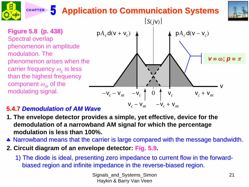
Signals_and_Systems_Simon Haykin amp Barry Van Veen
22
Application to Communication SystemsApplication to Communication SystemsCHAPTER
Figure 59 (p 438)Figure 59 (p 438)Envelope detector illustrated by (a) circuit diagram (b) AM wave input and (c) envelope detector output assuming ideal conditions
Signals_and_Systems_Simon Haykin amp Barry Van Veen
23
Application to Communication SystemsApplication to Communication SystemsCHAPTER
2) 2) The AM signal applied to the envelope is supplied by a voltage sThe AM signal applied to the envelope is supplied by a voltage source of ource of internal resistance internal resistance RRss
3) The load resistance 3) The load resistance RRll is large compared with the source resistance is large compared with the source resistance RRss During Duringthe charging process the time constant is effectively equathe charging process the time constant is effectively equal to l to RRssCC This time This time constant must be short compared with the carrier period 2constant must be short compared with the carrier period 2ππωωcc that is that is
2s
c
R πω
ltlt (515)
3 The discharging time constant is equal to RlCRRllCC must be large such that the capacitor discharges slowly but notmust be large such that the capacitor discharges slowly but not so so large that the capacitor voltage will not discharge at the maximlarge that the capacitor voltage will not discharge at the maximum rate um rate of change of the modulating wave ieof change of the modulating wave ie2 2
lc m
R Cπ πω ω
ltlt ltlt (516) ωm equiv message
bandwidth
clubs Output ripple can be removed by low-pass filter
Signals_and_Systems_Simon Haykin amp Barry Van Veen
24
Application to Communication SystemsApplication to Communication SystemsCHAPTER
55 55 Double SidebandDouble Sideband--Suppressed ModulationSuppressed Modulation1 In full AM carrier wave c(t) is completely independent of the message signal
m(t)
Transmission of carrier wave A waste of power
2 To overcome this shortcoming we may suppress the carrier component from the modulated wave resulting in double sideband-suppressed carrier(DSB-SC) modulation
3 DSB-SC modulated signal( ) ( ) ( ) cos( ) ( )c cs t c t m t A t m tω= = (517)
clubs This modulated signal undergoes a phase reversal whenever the messagesignal m(t) crosses zero as illustrated in Fig 510Fig 510(a)(a) Message signal Message signal (b)(b) DSBDSB--SC modulated wave resulting from multiplication of the message SC modulated wave resulting from multiplication of the message
signal by the sinusoidal carrier wave signal by the sinusoidal carrier wave
Signals_and_Systems_Simon Haykin amp Barry Van Veen
25
Application to Communication SystemsApplication to Communication SystemsCHAPTER
Figure 510 (p 440)Figure 510 (p 440)Double-sideband-suppressed carrier modulation (a) Message signal (b) DSB-SC modulated wave resulting from multiplication of the message signal by the sinusoidal carrier wave
551 551 FrequencyFrequency--Domain DescriptionDomain Description1 Fourier transform of modulated signal s(t)
1( ) [ ( ( )) ( ( ))]2 c c cS j A M j M jω ω ω ω ω= minus + + (518)
where M(jω) equiv Fourier transform of m(t) minus ωm le ω le ωmFig 511 (a) and (b)Fig 511 (a) and (b)
Signals_and_Systems_Simon Haykin amp Barry Van Veen
26
Application to Communication SystemsApplication to Communication SystemsCHAPTER
Figure 511 (p 441)Figure 511 (p 441)Spectral content of DSB-SC modulated wave (a) Magnitude spectrum of message signal (b) Magnitude spectrum of DSB-SC modulated wave consisting of upper and lower sidebands only
v equiv ω p equiv π
clubs The modulation process simply translates the spectrum of the message signal by plusmn ωc
clubs Transmission bandwidth = 2 ωm2 A device for achieving DSB-SC is called a product modulator or simply
multiplierFig 512 (a)Fig 512 (a) shows the block diagram of a product modulator
Signals_and_Systems_Simon Haykin amp Barry Van Veen
27
Application to Communication SystemsApplication to Communication SystemsCHAPTER
Figure 512 (p 441)Figure 512 (p 441)(a) Product modulator for generating the DSB-SC modulated wave (b) Coherent detector for demodulation of the DSB-SC modulated wave
v equiv ω p equiv π
552 552 Coherent DetectionCoherent Detection1 The message signal m(t) may be recovered from DSB-SC
Fig 512 (b)Fig 512 (b)ss((tt) ) timestimes locally generated sinusoidal wave = locally generated sinusoidal wave = vv((tt))vv((tt) filtered by a Low) filtered by a Low--pass filterpass filter
Local oscillator
2 The local oscillator should be exactly coherent or synchronized in both frequency and phase with the carrier wave c(t)
Signals_and_Systems_Simon Haykin amp Barry Van Veen
28
Application to Communication SystemsApplication to Communication SystemsCHAPTER
Coherent detection or synchronization demodulation3 Derivation for coherent detection
1) Local oscillator cos(ωct + φ )2) Product modulator output
( ) cos( ) ( )cos( ) cos( ) ( )
1 1cos( ) ( ) cos(2 ) ( )2 2
c
c c c
c c c
v t t s tA t t m t
A m t A t m t
ω φω ω φ
φ ω φ
= += +
= + +(519)
1 cos( ) ( )2 cA m tφ
1 cos(2 ) ( )2 c cA t m tω φ+
A scaled version of the original message signal m(t)
DSBDSB--SC modulated signal with carrier SC modulated signal with carrier frequency 2 frequency 2 ωωcc
3) Magnitude spectrum Fig 5134) To clear separate two component of v(t) the original carrier frequency ωc
must satisfy the condition
Signals_and_Systems_Simon Haykin amp Barry Van Veen
29
Application to Communication SystemsApplication to Communication SystemsCHAPTER
Figure 513 (p 442)Figure 513 (p 442)Magnitude spectrum of the product modulator output v(t) in the coherent detector of Fig 512(b)
v equiv ω p equiv π
2 c m mω ω ωminus gt c mω ωgt (520) ωωmm equivequiv message bandwidthmessage bandwidth
4 Specification of low-pass filter1) 1) The cutoff frequency must be The cutoff frequency must be ωωm m 2) The transition band must be 2) The transition band must be ωωm m ≦≦ ωω ≦≦ ωωc c ωωm m
Thus the overall output in Thus the overall output in Fig 512(b)Fig 512(b) is given byis given by1( ) cos( ) ( )2o cv t A m tφ= (521)
cosφ equiv attenuation factor
Signals_and_Systems_Simon Haykin amp Barry Van Veen
30
Application to Communication SystemsApplication to Communication SystemsCHAPTER
5 (1) Demodulated signal vo(t) is proportional to m(t) when the error phase φis a constant
(2) Demodulated signal is maximum when φ = 0 and has a minimum zero when φ = plusmn π2
Example 53 Sinusoidal DSB-SC ModulationConsider again the sinusoidal modulating signal
0 0( ) cos( )m t A tω=
( ) cos( )c cc t A tω=with amplitude A0 and frequency ω0 see Fig 514(a) The carrier wave is
with amplitude Ac and frequency ωc see Fig 514(b) Investigate the time-domain and frequency-domain characteristics of the corresponding DSB-SC modulated waveltltSolgtSolgt
clubs φ = plusmn π2 represents the quadrature null effect of the coherent detector
1 The modulated DSB-SC signal is defined by
0 0
0 0 0 0
( ) cos( ) cos( )1 1cos[( ) ] cos[( ) ]2 2
c c
c c c c
s t A A t t
A A t A A t
ω ω
ω ω ω ω
=
= + + minus
Signals_and_Systems_Simon Haykin amp Barry Van Veen
31
Application to Communication SystemsApplication to Communication SystemsCHAPTER
2 The Fourier transform of s(t) is given by
0 0 0
0 0
1( ) cos[ ( ) ( )]2
( ) ( )
c c c
c c
S j A Aω π δ ω ω ω δ ω ω ω
δ ω ω ω δ ω ω ω
= minus minus + + +
+ minus + + + minus
which consists of four weighted impulse functions at the frequencies ωc+ ω0-ωc- ω0 ωc- ω0 and- ωc+ ω0 as illustrated in the right-hand side of Fig Fig 514(c)514(c)
3 This Fourier transform differs from that depicted in the right-hand side of Fig Fig 56(c)56(c) for the corresponding example of full AM in one important respect The impulse functions at plusmn ωc due to the carrier are removed
4 Application of the sinusoidally modulated DSB-SC signal to the product modulator of Fig 512(b) yields the output (assuming φ = 0)
0 0 0
0 0 0 0 0
1( ) cos( ) cos[( ) ] cos[( ) ]21 cos[(2 ) ] cos( ) cos[(2 ) ] cos( )4
c c c c
c c c
v t A A t t t
A A t t t t
ω ω ω ω ω
ω ω ω ω ω ω
= + + minus
= + + + minus +
Signals_and_Systems_Simon Haykin amp Barry Van Veen
32
Application to Communication SystemsApplication to Communication SystemsCHAPTER
Figure 514 (p Figure 514 (p 443)443)Time-domain (on the left) and frequency-domain (on the right) characteristics of DSB-SC modulation produced by a sinusoidal modulating wave (a) Modulating wave (b) Carrier wave (c) DSB-SC modulated wave Note that ω= 2πƒ
v equiv ω p equiv π
Signals_and_Systems_Simon Haykin amp Barry Van Veen
33
Application to Communication SystemsApplication to Communication SystemsCHAPTER
5 The first two sinusoidal terms of v(t) are produced by the upper side frequency and the last two sinusoidal terms are produced by the lower side frequency
6 With ωcgt ω0 the first and third sinusoidal terms of frequencies 2ωc+ ω0 and 2ωc-ω0 respectively are removed by the low-pass filter of Fig 512(b)Fig 512(b) which leaves the second and fourth sinusoidal terms of frequency ω0 as the only output of the filter The coherent detector output thus reproduces the original modulating wave
7 Note however that this output appears as two equal terms one derived from the upper side frequency and the other from the lower side frequency We therefore conclude that for the transmission of the sinusoidal signal A0 cos(ω0t) only one side frequency is necessary (The issue will be discussed further in Section 57Section 57)
553 553 CostasCostas ReceiverReceiver1 Costas receiver Fig 515Fig 5152 This receiver consists of two coherent detector supplied with the same input
ie the incoming DSB-Sc wave
cos(2 ) ( )c cA f t m tπ but with individual local oscillator signals that are in phase duadrature with respect to each other
In-phase coherent detector (I-Channel) and quadrature-phase coherent detector (Q-Channel)
Signals_and_Systems_Simon Haykin amp Barry Van Veen
34
Application to Communication SystemsApplication to Communication SystemsCHAPTER
Figure 515 (p 445)Figure 515 (p 445)Costas receiver
v equiv ω p equiv π
Signals_and_Systems_Simon Haykin amp Barry Van Veen
35
Application to Communication SystemsApplication to Communication SystemsCHAPTER
56 56 QuadratureQuadrature--Carrier MultiplexingCarrier Multiplexing
Figure 516 (p 446)Figure 516 (p 446)Quadrature-carrier multiplexing system exploiting the quadrature null effect (a) Transmitter (b) Receiver assuming perfect synchronization with the transmitter
v equiv ω p equiv π
1 1 A A quadraturequadrature--carrier multiplexing or carrier multiplexing or quadraturequadrature--amplitude modulation (QAM) amplitude modulation (QAM) system enables two DSBsystem enables two DSB--SC modulated waves to occupy the same transmission SC modulated waves to occupy the same transmission bandwidth and yet it allows for their separation at the receivebandwidth and yet it allows for their separation at the receiver outputr output
BandwidthBandwidth--conservation schemeconservation scheme
Signals_and_Systems_Simon Haykin amp Barry Van Veen
36
Application to Communication SystemsApplication to Communication SystemsCHAPTER
2 Fig 5-16(a) Block diagram of the quadrature-carrier multiplexing systemFig 5-16(a) transmitter Fig 5-16(b) receiver
3 Multiplexed signal s(t)
(522) 1 2( ) ( ) cos( ) ( )sin( )c c c cs t A m t t A m t tω ω= +
where m1(t) and m2(t) denotes the two different message signals applied to the product modulations
clubsTransmission bandwidth = 2 ωm centered at ωc where ωm is the commonmessage bandwidth of m1(t) and m2(t)
4 The output of the top detector at receiver is 1
12 ( )cA m t
The output of the bottom detector at receiver is1
22 ( )cA m t
57 57 Other Variants of Amplitude Modulation Other Variants of Amplitude Modulation clubs Basic concept Full AM and DSB-SC rArr Wasteful of bandwidthclubs Given the amplitude and phase spectra of either lower or upper sideband
we can uniquely determine the other
Signals_and_Systems_Simon Haykin amp Barry Van Veen
37
Application to Communication SystemsApplication to Communication SystemsCHAPTER
clubs Single-sideband (SSB) modulation only one sideband is transmitted571 571 FrequencyFrequency--Domain Description of SSB ModulationDomain Description of SSB Modulation1 Consider a message signal m(t) with a spectrum M(jω) limited to the band
ωa le ω le ωb Fig 5-17 (a)2 DSB-SC modulated signal
( ) cos( )c cm t A tωtimes Fig 5-17 (b)
3 (1) Upper sideband the frequencies above ωc and below minus ωc(2) Upper sideband the frequencies below ωc and above minus ωc
Fig 5-17 (c)4 When only the lower sideband is transmitted the spectrum of the
corresponding SSB modulated wave is as shown in Fig 5-17 (d) 5 Advantages of SSB
(1) Reduced bandwidth requirement(2) Elimination of the high-power carrier waveDisadvantage od SSB(1) Cost and complexity of implementing both the transmitter and receiver
Signals_and_Systems_Simon Haykin amp Barry Van Veen
38
Application to Communication SystemsApplication to Communication SystemsCHAPTER
Figure 517 Figure 517 (p 447)(p 447)Frequency-domain characteristics of SSB modulation (a) Magnitude spectrum of message signal with energy gap from ndash ωa to ωa
(c) Magnitude spectrum of SSB modulated wave containing upper sideband only
(d) Magnitude spectrum of SSB modulated wave containing lower sideband only
(b) Magnitude spectrum of DSB-SC signal
v equiv ω p equiv π
Signals_and_Systems_Simon Haykin amp Barry Van Veen
39
Application to Communication SystemsApplication to Communication SystemsCHAPTER
6 Frequency-discrimination scheme for producing SSB modulation Fig 518clubs Bandpass filter is designed to pass the sideband selected for transmission
and suppress the remaining sidebandclubs Requirement in SSB signal the message signal applied to the product
modulator must have a energy gap in its spectrum Refer to Fig 517 (a)
Figure 518 (p 448)Figure 518 (p 448)System consisting of product modulator and bandpass filter for generating SSB modulated wave
v equiv ω p equiv π
572 572 TimeTime--Domain Description of SSB ModulationDomain Description of SSB Modulation1 Mathematical tool Hilbert transform
The Hilbert transform of a signal x(t) is defined by1 ( ) 1ˆ( ) ( )xx t d x t
t tτ τ
π τ πinfin
minusinfin= = lowast
minusint
Signals_and_Systems_Simon Haykin amp Barry Van Veen
40
Application to Communication SystemsApplication to Communication SystemsCHAPTER
The Fourier transform of 1(πt) is minus j times the signum function denoted
1 for 0sgn( ) 0 for 0
1 for 0
ωω ω
ω
+ gt⎧⎪= =⎨⎪minus lt⎩
2 Passing x(t) through a Hilbert transformer is equivalent to the combination of the following two operations in frequency domain1) Keeping X(jω)unchanged for all ω 2) Shifting areX(jω) (ie the phase spectrum of x(t)) by +90deg for negative
frequencies and minus 90deg for positive frequencies clubs Hilbert transformer = Wideband minus 90deg phase shifter 573 573 Vestigial Sideband ModulationVestigial Sideband Modulation1 When the message signal contains significant components at extremely
low frequencies the upper and lower sidebands meet at the carrier frequency
Using SSB is inappropriateUsing SSB is inappropriateEx TV signals or
wideband dataUsing VSB (Vestigial sideband) modulation is appropriateUsing VSB (Vestigial sideband) modulation is appropriate
Signals_and_Systems_Simon Haykin amp Barry Van Veen
41
Application to Communication SystemsApplication to Communication SystemsCHAPTER
2 VSB is a compromise between SSB and DSB-SC forms of modulationIn VSB modulation one sideband is passes almost completely whereas just a trace or vestige of the other sideband is retained
3 Fig 519 illustrates a VSB modulated wave s(t) in relation to the message signal m(t)
v equiv ω p equiv π
Figure 519 (p 449)Figure 519 (p 449)Spectral content of VSB modulated wave (a) Magnitude spectrum of message signal (c) Magnitude spectrum of VSB modulated wave containing a vestige of the lower sideband
clubs The lower sideband is modified into the vestigial sideband4 Transmission bandwidth of VSB modulated wave T m vω ω ω= + (523)
where ωm is the message bandwidth and ωu is the width of the vestigial sideband
Signals_and_Systems_Simon Haykin amp Barry Van Veen
42
Application to Communication SystemsApplication to Communication SystemsCHAPTER
5 Generation of VSB modulated wave Fig 520
Figure 520 (p 450)Figure 520 (p 450)System consisting of product modulator and sideband shaping filter for generating VSB modulated wave
v equiv ω p equiv π
Passing a DSBPassing a DSB--SC modulated wave through a sidebandSC modulated wave through a sideband--shaping filtershaping filter6 The sideband-shaping filter is designed so that the original message
spectrum M(jω) is reproduced on the demodulation as a result of the superposition of two spectra
1) The positive-frequency part of S(jω) (ie the Fourier transform of the transmitted signal s(t)) shifted downward in frequency by ωc
2) The negative-frequency part of S(jω) shifted upward in frequency by ωc
Fig 521 A reflection of the vestige of the lower sideband makes up for the missing parts of the upper sideband
Signals_and_Systems_Simon Haykin amp Barry Van Veen
43
Application to Communication SystemsApplication to Communication SystemsCHAPTER
Figure 521 (p 450)Figure 521 (p 450)Superposition of the two spectra shown in parts (a) and (b) of the figure results in the original message spectrum (shown dashed) upon demodulation
58 58 PulsePulse--Amplitude Modulation Amplitude Modulation clubs Basic concept
Basic role in the operation of AM Frequency-shiftingBasic role in the operation of PAM Sampling
581 581 Sampling RevisitedSampling Revisited1 Sampling theorem
In view point of PAMIn view point of PAM
Signals_and_Systems_Simon Haykin amp Barry Van Veen
44
Application to Communication SystemsApplication to Communication SystemsCHAPTER
1) A band-limited signal of finite energy that has no radian frequency components higher than ωm is uniquely determined by the values of the signal at instants of time separated by π ωm seconds
2) A band-limited signal of finite energy that has no radian frequency components higher than ωm may be completely recovered from a knowledge of its samples taken at the rate of ωm π per seconds
clubs Part 1) rArr Be exploited in the transmitter of a PAM clubs Part 2) rArr Be exploited in the Receiver of a PAM2 To combat the effects of aliasing in practice we use two corrective measures1) Prior to sampling a low-pass antialiasing filter is used to attenuate those high-
frequency components of the signal which lie outside the band of interest2) The filtered signal is sampled at a rate slightly higher than the Nyquist rate3 Generation of a PAM signal Fig 522Fig 522Example 54 Telephonic CommunicationThe highest frequency component of a speech signal needed for telephonic communication is about 31 kHz Suggest a suitable value for the sampling rate ltltSolgtSolgt
Signals_and_Systems_Simon Haykin amp Barry Van Veen
45
Application to Communication SystemsApplication to Communication SystemsCHAPTER
Figure 522 (p 451)Figure 522 (p 451)System consisting of antialiasing filter and sample-and-hold circuit for converting a message signal into a flattopped PAM signal
1 The highest frequency component of 31 kHz corresponds to 362 10 radsmω π= times
Correspondingly the Nyquist rate is
62 kHzmωπ
=
2 A suitable value for the sampling rate-one slightly higher than the Nyquistrate-may be 8 kHz a rate that is the international standard for telephone speech signals
Signals_and_Systems_Simon Haykin amp Barry Van Veen
46
Application to Communication SystemsApplication to Communication SystemsCHAPTER
582 582 Mathematical Description of PAMMathematical Description of PAM1 The carrier wave used in PAM consists of a sequence of short pulses of
fixed duration in terms of which PAM is formally defined as followsPAM is a form of pulse modulation in which the amplitude of the PAM is a form of pulse modulation in which the amplitude of the pulsed carrier is pulsed carrier is varied in accordance with instantaneous sample values of the mesvaried in accordance with instantaneous sample values of the message signalsage signal the duration of the pulsed carrier is maintained constant throughout
Fig 523Fig 523
Figure 523 (p452) Figure 523 (p452) Waveform of flattopped PAM signal with pulse duration T0 and sampling period Ts
Signals_and_Systems_Simon Haykin amp Barry Van Veen
47
Application to Communication SystemsApplication to Communication SystemsCHAPTER
2 Mathematical representation of the PAM
( ) [ ] ( )sn
s t m n b t nTinfin
=minusinfin
= minussum (524) s(t) equiv PAM signal m(t) equiv
message signal
Ts equiv sampling period m[n] equiv the values of m(t) at t = nTs h(t) equiv rectangular pulse of the unit amplitude and duration T0
3 Rectangular pulse
01 0( )
0 otherwiset T
h tlt lt⎧
= ⎨⎩
(525) Fig 524 (a)Fig 524 (a)
clubs Eq (524) is a sample-and-hold operationAnalogous to zeroAnalogous to zero--orderorder--holdhold--
based reconstruction in Sec 46based reconstruction in Sec 46
差異差異hh((tt) ) 的的TTss與與TT00
4 Impulse-sampled version of message signal m(t)
( ) [ ] ( )sn
m t m n t nTδ δinfin
=minusinfin
= minussum (526)
5 PAM signal( ) [ ] ( )
( ) ( )
sn
s t m n b t nT
m t b tδ
infin
=minusinfin
= minus
=
sum(527)
Convolution of impulse-sampled version mδ(t) and h(t)
Time domain Time domain operationoperation
Signals_and_Systems_Simon Haykin amp Barry Van Veen
48
Application to Communication SystemsApplication to Communication SystemsCHAPTER
Figure 524 (p 453)(a) Rectangular pulse h(t) of unit amplitude and duration T0 (b) Magnitude spectrum |H(jω)| and phase spectrum argH(jω) of pulse h(t)
v equiv ω p equiv π
Signals_and_Systems_Simon Haykin amp Barry Van Veen
49
Application to Communication SystemsApplication to Communication SystemsCHAPTER
6 FT of PAM signal( ) ( ) ( )S j M j H jδω ω ω= (528)
where( ) ( )FTS j s tω larr⎯rarr ( ) ( )FTM j m tδ δω larr⎯rarr ( ) ( )FTH j h tω larr⎯rarr
7 Impulse sampling of the message signal m(t) introduces periodicity into the spectrum as given by
1( ) ( ( ))sks
M j M j kTδ ω ω ω
infin
=minusinfin
= minussum (529) 1Ts equiv sampling rate ωs = 2πTs rads
1( ) ( ( )) ( )sks
S j M j k H jT
ω ω ω ωinfin
=minusinfin
= minussum (530)
( ) ( )FTM j m tω larr⎯rarrwhere
clubs Suppose that m(t) is strictly band limited and that the sampling rate 1Ts is greater than the Nyquist rate Then passing s(t) through a reconstruction filter chosen as an ideal low-pass filter with cutoff frequency ωm and gain Ts we find that the spectrum of the resulting filter output is equal to M(jω)H(jω)
Signals_and_Systems_Simon Haykin amp Barry Van Veen
50
Application to Communication SystemsApplication to Communication SystemsCHAPTER
8 From Eq (525) we find that0 2
0 0( ) sin ( (2 )) j TH j T c T e ωω ω π minus= (531) Fig 524(b) magnitude and phase of H(jω)
clubs Using PAM to represent a continuous-time message signal we introduce amplitude distortion as well as a delay of T02
clubs The frequency distortion caused by the use of flat-topped sampled in the generation of a PAM wave illustrated in Fig 523Fig 523 is referred to as the aperture effect
583 583 Demodulation of PAM SignalDemodulation of PAM Signal1 Reconstruction scheme Fig 525Fig 525
Figure 525 (p 454)Figure 525 (p 454)System consisting of low-pass interpolation filter and equalizer for reconstructing a message signal from its flattopped sampled version
clubs The system consists of low-pass interpolation filter and equalizer connected in cascade
Signals_and_Systems_Simon Haykin amp Barry Van Veen
51
Application to Communication SystemsApplication to Communication SystemsCHAPTER
2 The cutoff frequency of low-pass filter = the highest frequency ωm of message signal
3 The equalizer is used to correct the aperture effect due to flat-topped sampling in the sample-and-hold circuit
4 The equalizer has the effect of decreasing the in-band loss of the interpolation filter as frequency increases in such a manner as to compensate for the aperture effect
5 Amplitude response of equalizer
0
0 0 0 0
1 1 1| ( ) | | sinc( 2) | 2 | sin( 2) |
TH j T T T T
ωω ω ω
= =
Frequency response Eq (531)
Example 55 Equalization for PAM TransmissionThe duty cycle in a PAM signal namely T0 Ts is 10 Evaluate the peak amplification required for equalizationltltSolgtSolgt1 At ωm = π Ts which corresponds to the highest frequency component of the
message signal for a sampling rate equal to the Nyquist rate we find from Eq (531) that the magnitude response of the equalizer at ωm normalized to that at zero frequency is
Signals_and_Systems_Simon Haykin amp Barry Van Veen
52
Application to Communication SystemsApplication to Communication SystemsCHAPTER
Figure 526 (p 455)Figure 526 (p 455)Normalized equalization (to compensate for aperture effect) plotted against the duty cycle T0Ts
Signals_and_Systems_Simon Haykin amp Barry Van Veen
53
Application to Communication SystemsApplication to Communication SystemsCHAPTER
0
0 0
( 2)( )1sin (05 ) sin[( 2)( )]
s
s s
T Tc T T T T
ππ
=
where the ratio T0 Ts is equal to the duty cycle of the sampling pulses 2 In Fig 526Fig 526 this result is plotted as a function of the duty cycle T0 Ts Ideally it
should be equal to unity for all values of T0 Ts 3 For a duty cycle of 10 it is equal to 10041 It follows that for duty cycles of less
than 10 the magnitude equalization required is less than 10041 in which case the aperture effect is usually considered to be negligible
59 59 Multiplexing Multiplexing clubs Three basic types of multiplexing1 Frequency-division multiplexing in which the signals are separated by
allocating them to different frequency bands This is illustrated in Fig 527(a) for the case of six different message signals Frequency-division multiplexing favors the use of CW modulation where each message signal is able to use the channel on a continuous-time basis
2 Time-division multiplexing wherein the signals are separated by allocating them to different time slots within a sampling interval
Signals_and_Systems_Simon Haykin amp Barry Van Veen
54
Application to Communication SystemsApplication to Communication SystemsCHAPTER
This second type of multiplexing is illustrated in Fig 527(b) for the case of six different message signals Code-division multiplexing which relies on the assignment of different codes to the individual users of the channel
3 Code-division multiplexing which relies on the assignment of different codes to the individual users of the channel
591 591 FrequencyFrequency--Domain Multiplexing (FDM)Domain Multiplexing (FDM)1 Block diagram Fig 528Fig 5282 Incoming message signals low-pass variety3 Low-pass filter to remove high-frequency components such that the signal
in each channel does not disturb each other4 MOD (modulator) shift the frequency ranges of the signals so as to occupy
mutually exclusive frequency intervalsSSB is often used in this stageEx Voice input is usually assigned a bandwidth of 4 kHz
5 Band-pass filters are used to restrict the band of each modulated wave to its prescribed range
6 Band-pass filters in receiver separate the message signals7 DEM (demodulator) to recover signalsclubs FDM in Fig 528 operates in only one direction
Signals_and_Systems_Simon Haykin amp Barry Van Veen
55
Application to Communication SystemsApplication to Communication SystemsCHAPTER
Figure 527 (p 456)Figure 527 (p 456)Two basic forms of multiplexing (a) Frequency-division multiplexing (with guardbands) (b) Time-division multiplexing no provision is made here for synchronizing pulses
Signals_and_Systems_Simon Haykin amp Barry Van Veen
56
Application to Communication SystemsApplication to Communication SystemsCHAPTER
Figure 528 (p 457)Figure 528 (p 457)Block diagram of FDM system showing the important constituents of the transmitter and receiver
Signals_and_Systems_Simon Haykin amp Barry Van Veen
57
Application to Communication SystemsApplication to Communication SystemsCHAPTER
Example 56 SSB-FDM System
ltltSolgtSolgt
An FDM system is used to multiplex 24 independent voice signals SSB modulation is used for the transmission Given that each voice signal is allotted a bandwidth 4kHz calculate the overall transmission bandwidth of the channel
With each voice signal allotted a bandwidth of 4 kHz the use of SSB modulation requires a bandwidth of 4 kHz for its transmission Accordingly the overall transmission bandwidth provided by the channel is 24 X 4 = 96 kHz 592 592 TimeTime--Domain Multiplexing (TDM)Domain Multiplexing (TDM)clubs Basic to the operation of a TDM system is the sampling theoremclubs The transmission of the message samples engages the transmission channel for
only a fraction of the sampling interval on a periodic basis equal to the width T0 of a PAM modulating pulse
1 Block diagram Fig 529Fig 5292 Commutator is usually implemented by means of electronic switching
circuitry3 The function of commutator is two folds
Signals_and_Systems_Simon Haykin amp Barry Van Veen
58
Application to Communication SystemsApplication to Communication SystemsCHAPTER
Figure 529 (p 458)Figure 529 (p 458)Block diagram of TDM system showing the important constituents of the transmitter and receiver
(1) To take a narrow sample of each of the M input message signals at a rate 1Tsthat is slightly higher than ωcπ where ωc is the cutoff frequency of the input low-pass filter
(2) To sequentially interleave these M samples inside a sampling interval Ts4 Pulse modulator transform the multiplexed signal into a form suitable for
transmission over the common channel
Signals_and_Systems_Simon Haykin amp Barry Van Veen
59
Application to Communication SystemsApplication to Communication SystemsCHAPTER
clubs The use of time-division multiplexing introduces a bandwidth expansion factor M because the scheme must squeeze M samples derived from M independent message sources into a time slot equal to one sampling interval
5 Pulse demodulator performs the inverse operation of the pulse modulator6 Decommutator distributes the narrow samples produced by pulse demodulator to the appropriate low-pass reconstruction filter7 Synchronization between the timing operations of the transmitter and
receiver in a TDM system is essential for satisfactory performance of the system
Inserting an extra pulse into each sampling interval on a regular basisBandwidth expansion factor is increased to M + 1
clubs The TDM system is hghly sensitive to the dispersion in the common transmission channel
Example 57 Comparison of TDM with FDMATDM system is used to multiplex four independent voice signals using PAM Each voice signal is sampled at the rate of 8 kHz The system incorporates a synchronizing pulse train for its proper operation
Signals_and_Systems_Simon Haykin amp Barry Van Veen
60
Application to Communication SystemsApplication to Communication SystemsCHAPTER
(a) Determine the timing relationships between the synchronizing pulse train and the impulse trains used to sample the four voice signals
(b) Calculate the transmission bandwidth of the channel for the TDM system and compare the result with a corresponding FDM system using SSBmodulation
ltltSolgtSolgt(a) The sampling period is
31 125 s
8 10sT s μ= =times
In this example the number of voice signals is M = 4 Hence dividing the sampling period of 125 μs among these voice signals and the synchronizing pulse train we obtain the time slot allocated to each one of them
0 1125 25 s
5
sTTM
μ
=+
= =
Signals_and_Systems_Simon Haykin amp Barry Van Veen
61
Application to Communication SystemsApplication to Communication SystemsCHAPTER
Figure 530Figure 530 shows the timing relationships between the synchronizing pulse train and the four impulse trains used to sample the different voice signals in a single frame Each frame includes time slots of common duration T0 = 25 μs which are allocated to the pulse-modulated signals and synchronizing pulse
Figure 530 (p 459)Figure 530 (p 459)Composition of one frame of a multiplexed PAM signal incorporating four voice-signals and a synchronizing pulse
Signals_and_Systems_Simon Haykin amp Barry Van Veen
62
Application to Communication SystemsApplication to Communication SystemsCHAPTER
(b) As a consequence of the time-bandwidth product (see Section 317) there is an inverse relationship between the duration of a pulse and the bandwidth (ie cutoff frequency) of the channel needed for itstransmission Accordingly the overall transmission bandwidth of the channel is
0
21 1 MHz 40 kHz
25
TTf
T
ωπ
=
= = =
In contrast the use of an FDM system based on SSB modulation requires a channel bandwidth equal to M times that of a single voice signal-that is 4 X 4 = 16 kHz Thus the use of PAM-TDM requires a channel bandwidth that is 40 16 = 25 times that of SSB-FDMIn practice pulse-code modulation is commonly used as the method of modulation for TDM this results in a further increase in channel bandwidth depending on the length of the code word used in the digital representation of each pulse in the PAM signal
Signals_and_Systems_Simon Haykin amp Barry Van Veen
63
Application to Communication SystemsApplication to Communication SystemsCHAPTER
510 510 Pulse and Group Delays Pulse and Group Delays 1 Whenever a signal is transmitted through a dispersive (ie frequency
selective) system some delay is introduced into the output signal in relation to the input signal
2 The delay is determined by the phase response of the system3 Phase response of a dispersive communication channel
( ) arg ( )H jφ ω ω= (532)
A signal is transmitted through the channel at a frequency ωc The signal received at the channel lags the transmitted signal by φ(ωc) The time delay is called phase delay formally defined as
( )cp
c
φ ωτω
= minus (533)
The phase delay is not necessarily the true signal delayclubs Case study for DSB-SC1 Transmitted signal
0( ) cos( ) cos( )cs t A t tω ω= (534)
ωc equiv carrier frequency ω0 equiv sinusoidal modulation frequency
A = AcA0
Signals_and_Systems_Simon Haykin amp Barry Van Veen
64
Application to Communication SystemsApplication to Communication SystemsCHAPTER
1 21 1( ) cos( ) cos( )2 2
s t A t A tω ω= +
1 0cω ω ω= + (535) where
2 0cω ω ω= minus (536)
Upper frequency
Lower frequency
2 Let the s(t) be transmitted through the channel with phase response φ (ω) Accordingly the signal received at the channel output is
1 1 2 21 1( ) cos( ( )) cos( ( ))2 2
y t A t A tω φ ω ω φ ω= + + +
1 2 1 20
( ) ( ) ( )1 ( )( ) cos cos2 2cy t A t tφ ω φ ω φ ω φ ωω ω+⎛ ⎞ ⎛ ⎞= + +⎜ ⎟ ⎜ ⎟
⎝ ⎠ ⎝ ⎠(537)
3 Two observations from Eq (537)1) The carrier component at frequency ωc in y(t) lags its counterpart in s(t) by
frac12 (φ (ω1) + φ (ω2)) which represents a time delay equal to
1 2 1 2
c 1 2
( )+ ( ) ( )+ ( )2 +
φ ω φ ω φ ω φ ωω ω ω
minus = minus (538)
Signals_and_Systems_Simon Haykin amp Barry Van Veen
65
Application to Communication SystemsApplication to Communication SystemsCHAPTER
2) The message component at frequency ω0 in y(t) lags its counterpart in s(t) by frac12 (φ (ω1) minus φ (ω2)) which represents a time delay equal to
1 2 1 2
0 1 2
( ) ( ) ( ) ( )2
φ ω φ ω φ ω φ ωω ω ωminus minus
minus = minusminus
(539)
4 Suppose that ω0 lt ωc rArr the side frequencies are close together with ω c between them Such a modulated signal is said to be a narrowband signal The phase response φ (ω) in the vicinity of ω = ωc is approximated by two-term Taylor series expansion
( )( ) ( ) ( )c
c cd
d ω ω
φ ωφ ω φ ω ω ωω =
= + times minus (540)
Phase delay = ( ) c cφ ω ωminus
5 The time delay introduced by the message signal (ie he ldquoenveloperdquo of the modulated signal) is given by
( )
c
gd
d ω ω
φ ωτω =
= minus (541) The time delay τg is called the
envelope delay or group delay
Signals_and_Systems_Simon Haykin amp Barry Van Veen
66
Application to Communication SystemsApplication to Communication SystemsCHAPTER
6 When a modulated signal is transmitted through a communication channel there are two different delays to be considered1) The carrier or phase delay τp defined by Eq (533)2) The envelope or group delay τg defined by Eq (541)
clubs The group delay is the true signal delay
Example 58 Phase and Group Delays for Ban-pass Channel
ltltSolgtSolgt
The phase response of a band-pass communication channel is defined by 2 2
1( ) tan c
c
ω ωφ ωωω
minus ⎛ ⎞minus= minus ⎜ ⎟
⎝ ⎠The signal s(t) defined in Eq (534) is transmitted through this channel with
475 radscω = 0 025 radsω =andCalculate (a) the phase delay and (b) the group delay
(a) At ω = ωc φ (ωc) = 0 According to Eq (533) the phase delay τ p is zero (b) Differentiating φ (ω) with respect to ω we get
Signals_and_Systems_Simon Haykin amp Barry Van Veen
67
Application to Communication SystemsApplication to Communication SystemsCHAPTER
2 2
2 2 2 2 2
( )( )( )
c c
c c
dd
ω ω ωφ ωω ω ω ω ω
+= minus
+ minus
Using thing result in Eq (541) we find that the group delay is 2 2 04211
475gc
sτω
= = =
1 One waveform shown as a solid curve was obtained by multiplying the transmitted signal s(t) by the carrier wave cos(ωct)
2 The second waveform shown as a dotted curve was obtained by multiplying the received signal y(t) by the carrier wave cos(ωct)
To display the results obtained in parts (a) and (b) in graphical form Fig 531Fig 531shows a superposition of two waveforms obtained as follows
The figure clearly shows that the carrier (phase) delay τ p is zero and the envelope of the received signal y(t) is lagging behind that of the transmitted signal by τs seconds For the presentation of waveforms in this figure we purposely did not use a filter to suppress the high frequency components resulting from the multiplications described under points 1 and 2 because of the desire to retain a contribution due to the carrier for display
Signals_and_Systems_Simon Haykin amp Barry Van Veen
68
Application to Communication SystemsApplication to Communication SystemsCHAPTER
Figure 531 Figure 531 (p 463)(p 463)Highlighting the zero carrier delay (solid curve) and group delay τg (dotted curve) which are determined in accordance with Example 58
Signals_and_Systems_Simon Haykin amp Barry Van Veen
69
Application to Communication SystemsApplication to Communication SystemsCHAPTER
clubs Not also that the separation between the upper side frequency ω1 = ωc + ω0 = 500 rads and the lower side frequency ω2 = ωc minus ω0 = 450 rads is about 10 of the carrier frequency ωc = 475 rads which justifies referring to the modulated signal in this example as a narrowband signal
5101 5101 Some Practical ConsiderationsSome Practical Considerationsclubs What is the practical importance of group delay 1 Eq (541) for determining group delay applies strictly to narrowband
modulated signal2 The message bandwidth may be comparable to the carrier frequency In
this situation the group delay is formulated as a frequency-dependent parameter ie ( )d( )g d
φ ωτ ωω
= minus (542)
3 When a wideband modulated signals transmitted through a dispersive channel the frequency components of the message signal are delayed by different amounts at the channel output
Delay distortionFig 532Fig 532 Group delay response of voice-grade telephone channel
Signals_and_Systems_Simon Haykin amp Barry Van Veen
70
Application to Communication SystemsApplication to Communication SystemsCHAPTER
Figure 532 (p 464)Group delay response of voice-grade telephone channel (Adapted from J C Bellamy Digital Telephony Wiley 1982)
511 511 Exploring Concepts with MATLABExploring Concepts with MATLAB5111 5111 Full AMFull AMclubs Sinusoidal modulation
clubs To reconstruct a faithful version of the original message signal in the receiver we have to use a delay equalizer
0( ) [1 cos( )]cos( )c cs t A t tμ ω ω= +1 AM experiment
1cA =
08 radscω π= 0 01 radsω π=Carrier amplitude
Carrier frequency Modulation amplitude
Signals_and_Systems_Simon Haykin amp Barry Van Veen
71
Application to Communication SystemsApplication to Communication SystemsCHAPTER
2 We wish to display and analyze 10 full cycles of the AM wave corresponding to a total duration of 200 s Choosing a sampling rate 1Ts = 10 Hz we have a total of N = 2000 time samples The frequency band of interest is minus 10 π ≦ ω ≦ 10 π Since the separation between the carrier and either side frequency is equal to the modulation frequency ω0 = 01 π rads we would like to have a frequency resolution ωr = 001π rads To achieve this resolution we require the following number of frequency samples (see Eq (442))
20 2000001
s
r
M ω πω π
ge = =
3 We therefore choose M = 2000 To approximate the Fourier transform of the AM wave s(t) we may use a 2000-point DTFS The only variable in the AM experiment is the modulation factor μ with respect to which we wish to investigate three different situationsμ = 05 corresponding to under-modulationμ = 10 for which the AM system is on the verge of over-modulationμ = 20 corresponding to over-modulation
Signals_and_Systems_Simon Haykin amp Barry Van Veen
72
Application to Communication SystemsApplication to Communication SystemsCHAPTER
4 MATLAB commandsAc = 1 carrier amplitudewc = 08pi carrier frequencyw0 = 01pi modulation frequencymu = 05 modulation factort = 0011999s = Ac(1 + mucos(w0t))cos(wct)plot(ts)Smag = abs(fftshift(fft(s2000)))2000 Smag denotes the magnitude specturm of the AM wavew = 10[-1000999]2pi2000plot(wSmag)axis ([-30 30 0 08])
5 5 μμ = 05 = 05 case case Fig 533Fig 533μμ = 10 case = 10 case Fig 534Fig 534μμ = 20 case = 20 case Fig 535Fig 535
Discussion see pp 466-469 textbook
Signals_and_Systems_Simon Haykin amp Barry Van Veen
73
Application to Communication SystemsApplication to Communication SystemsCHAPTER
-30 -20 -10 0 10 20 300
02
04
06
0 50 100 150 200-2
-1
0
1
2
2 22 24 26 28 3
02
04
06
(a) Time (s)
Time domain
Frequency domain
(b) Frequency (rads)
Frequency domain
Frequency (rads)
Figure 533 (p 466)Amplitude modulation with 50 modulation (a) AM wave (b) magnitude spectrum of the AM wave and (c) expanded spectrum around the carrier frequency
μμ = 05 = 05 casecase
Signals_and_Systems_Simon Haykin amp Barry Van Veen
74
Application to Communication SystemsApplication to Communication SystemsCHAPTER
Figure 534 (p 467)Figure 534 (p 467)Amplitude modulation with 100 modulation (a) AM wave (b) magnitude spectrum of the AM wave and (c) expanded spectrum around the carrier frequency
Signals_and_Systems_Simon Haykin amp Barry Van Veen
75
Application to Communication SystemsApplication to Communication SystemsCHAPTER
Figure 535 (p 468)Amplitude modulation with 200 modulation (a) AM wave (b) magnitude spectrum of the AM wave and (c) expanded spectrum around the carrier frequency
Signals_and_Systems_Simon Haykin amp Barry Van Veen
76
Application to Communication SystemsApplication to Communication SystemsCHAPTER
5112 5112 DSBDSB--SC ModulationSC Modulation1 Sinusoidal modulation
0 0( ) cos( ) cos( )c cs t A A t tω ω=
2 MATLAB commands
Ac = 1 carrier amplitudewc = 08pi carrier frequency in radsA0 = 1 amplitude of modulating signalw0 = 01pi frequency of modulating signalt = 011999s = AcA0cos(wct)cos(w0t)plot(ts)Smag = abs(fftshift(fft(s2000)))2000w = 10[-1000999]2pi2000plot(wSmag)
3 3 DSBDSB--SC modulated waveSC modulated wave Fig 536Fig 536 Discussion see pp 466-469 textbook
4 Output of the product modulator in Fig 512 (b) with φ = 0
Signals_and_Systems_Simon Haykin amp Barry Van Veen
77
Application to Communication SystemsApplication to Communication SystemsCHAPTER
Figure 536 (p 469)DSB-SC modulation (a) DSB-SC modulated wave (b) magnitude spectrum of the modulated wave and (c) expanded spectrum around the carrier frequency
Signals_and_Systems_Simon Haykin amp Barry Van Veen
78
Application to Communication SystemsApplication to Communication SystemsCHAPTER
( ) ( ) cos( )cv t s t tω=
5 MATLAB commandsgtgt v = scos(wct)
6 Fig 537 (a) waveforms of v(t) Fig 537 (b) magnitude spectrum which readily shows that v(t) consists of the following components1) A sinusoidal component with frequency 01π rads representing the
modulating wave2) A new DSB-SC modulated wave with double carrier frequency of 16π rads
in actuality the side frequencies of this modulated wave are located at 15πand 17π rads
1) The frequency of the modulating wave lies inside the passband of the filter2) The upper and lower side frequencies of the new DSB-SC modulated wave
lie inside the stopband of the filter
Accordingly we may recover the sinusoidal modulating signal by passing v(t) through low-pass filter with the following requirements
Signals_and_Systems_Simon Haykin amp Barry Van Veen
79
Application to Communication SystemsApplication to Communication SystemsCHAPTER
Figure 537 (p 470)Coherent detection of DSB-SC modulated wave (a) and (b) Waveform and magnitude spectrum of signal produced at the output of produce modulator (c) and (d) waveform and magnitude spectrum of low-pass filter output
Signals_and_Systems_Simon Haykin amp Barry Van Veen
80
Application to Communication SystemsApplication to Communication SystemsCHAPTER
The issue of how to design a filter with these requirements will be considered in detail in Chapter 8 For the present it suffices to say that the preceding requirements can be met by using the following MATLAB commands
gtgt [ba] = butter(30025)gtgt output = filter(bav)
The first command produces s special type of filter called a Butterworth filter For the experiment considered here the filter order is 3 and its normalized cutoff frequency of 0025 is calculated as follows
Actual cutoff frequency of filter 025 radsHalf the sampling rate 10 rads
0025
ππ
=
=
The second command computes the filterrsquos output in response to the product modulator output v(t) (We will revisit the design of this filter in Chapter 8) Figure 537(c) displays the waveform of the low-pass filter output this waveform represents a sinusoidal signal of frequency 005 Hz an observation that is confirmed by using the ffr command to approximate the spectrum of the filter output The result of the computation is shown in Fig 537(d)Fig 537(d)
Signals_and_Systems_Simon Haykin amp Barry Van Veen
81
Application to Communication SystemsApplication to Communication SystemsCHAPTER
7 In Fig 538 we explore another aspect of DSB-SC modulation namely the effect of varying the modulation frequency Figure 538(a) shows five cycles of a DSB-SC modulated wave that has the same carrier frequency as that in Fig 536(a) but the modulation frequency has been reduced to 0025 Hz( ie a radian frequency of 005π) Figure 538(b) shows the magnitude spectrum of this second DSB-SC modulated wave and its zoomed-in version is shown in Fig 538(c) Comparing this latter figure with Fig 536(c) we see clearly that decreasing the modulation frequency has the effect of moving the upper and lower side frequencies closer together which is consistent with modulation theory
5113 5113 Phase and Group DelayPhase and Group Delay1 In Example 58 we studied the phase and group delays for a band-pass
channel with phase response 2 2
1( ) tan c
c
ω ωφ ωωω
minus ⎛ ⎞minus= minus ⎜ ⎟
⎝ ⎠2 At ω = ωc the phase delay is τ p = 0 and the group delay is τ s = 04211s One
of the wave forms displayed in Fig 531Fig 531 is
1( ) ( ) cos( )cx t s t tω=
Signals_and_Systems_Simon Haykin amp Barry Van Veen
82
Application to Communication SystemsApplication to Communication SystemsCHAPTER
Figure 538 (p 472)Effect of varying the modulation frequency compared with that in Fig 537 (a) and (b) Waveform and magnitude spectrum of DSB-SC modulated wave with a modulation frequency one-half that used in Fig 536 (c) expanded spectrum around the carrier frequency
Signals_and_Systems_Simon Haykin amp Barry Van Veen
83
Application to Communication SystemsApplication to Communication SystemsCHAPTER
where (see page 461)
1 2( ) [cos( ) cos( )]2As t t tω ω= +
and ω1 = ωc + ω0 and ω2 = ωc - ω0 The waveform shown in the figure as a solid curve is a plot of x1(t) The other waveform also displayed in Fig 531Fig 531 is
2
1 1 2 2
( ) ( ) cos( )
[cos( ( )) cos( ( ))]cos( )2
c
c
x t y t tA t t t
ω
ω φ ω ω φ ω ω
=
= + + +
where the angle φ (ω1) and φ (ω2) are the values of the phase response φ (ω) at ω = ω1 and ω = ω2 respectively The waveform shown as a dotted curve in the figure is a plot of x2(t)
3 The generation of x1(t) and x2(t) in MATLAB is achieved with the following commands with A2 set equal to unity
Signals_and_Systems_Simon Haykin amp Barry Van Veen
84
Application to Communication SystemsApplication to Communication SystemsCHAPTER
wc = 475w0 = 025w1 = wc + w0w2 = wc - w0t = -10 0001 10o1 = -atan((w1^2 - wc^2)(w1wc))o2 = -atan((w2^2 - wc^2)(w2wc))s = cos(w1t) + cos(w2t)y = cos(w1t + o1) + cos(w2t + o2)x1 = scos(478t)x2 = ycos(475t)plot(tx1b)hold on plot(tx2k)hold offxlabel(Time)ylabel(Amplitude)
Note that we have set (A2) = 1 for convenience of presentation The function atan in the first two commands returns the arctangent Note also that the computation of both x1 and x2 involve element-by-element multiplications ndash hence the use of period followed by an asterisk
Signals_and_Systems_Simon Haykin amp Barry Van Veen
85
Application to Communication SystemsApplication to Communication SystemsCHAPTER
Signals_and_Systems_Simon Haykin amp Barry Van Veen
86
Application to Communication SystemsApplication to Communication SystemsCHAPTER
Signals_and_Systems_Simon Haykin amp Barry Van Veen
87
Application to Communication SystemsApplication to Communication SystemsCHAPTER
Signals_and_Systems_Simon Haykin amp Barry Van Veen
24
Application to Communication SystemsApplication to Communication SystemsCHAPTER
55 55 Double SidebandDouble Sideband--Suppressed ModulationSuppressed Modulation1 In full AM carrier wave c(t) is completely independent of the message signal
m(t)
Transmission of carrier wave A waste of power
2 To overcome this shortcoming we may suppress the carrier component from the modulated wave resulting in double sideband-suppressed carrier(DSB-SC) modulation
3 DSB-SC modulated signal( ) ( ) ( ) cos( ) ( )c cs t c t m t A t m tω= = (517)
clubs This modulated signal undergoes a phase reversal whenever the messagesignal m(t) crosses zero as illustrated in Fig 510Fig 510(a)(a) Message signal Message signal (b)(b) DSBDSB--SC modulated wave resulting from multiplication of the message SC modulated wave resulting from multiplication of the message
signal by the sinusoidal carrier wave signal by the sinusoidal carrier wave
Signals_and_Systems_Simon Haykin amp Barry Van Veen
25
Application to Communication SystemsApplication to Communication SystemsCHAPTER
Figure 510 (p 440)Figure 510 (p 440)Double-sideband-suppressed carrier modulation (a) Message signal (b) DSB-SC modulated wave resulting from multiplication of the message signal by the sinusoidal carrier wave
551 551 FrequencyFrequency--Domain DescriptionDomain Description1 Fourier transform of modulated signal s(t)
1( ) [ ( ( )) ( ( ))]2 c c cS j A M j M jω ω ω ω ω= minus + + (518)
where M(jω) equiv Fourier transform of m(t) minus ωm le ω le ωmFig 511 (a) and (b)Fig 511 (a) and (b)
Signals_and_Systems_Simon Haykin amp Barry Van Veen
26
Application to Communication SystemsApplication to Communication SystemsCHAPTER
Figure 511 (p 441)Figure 511 (p 441)Spectral content of DSB-SC modulated wave (a) Magnitude spectrum of message signal (b) Magnitude spectrum of DSB-SC modulated wave consisting of upper and lower sidebands only
v equiv ω p equiv π
clubs The modulation process simply translates the spectrum of the message signal by plusmn ωc
clubs Transmission bandwidth = 2 ωm2 A device for achieving DSB-SC is called a product modulator or simply
multiplierFig 512 (a)Fig 512 (a) shows the block diagram of a product modulator
Signals_and_Systems_Simon Haykin amp Barry Van Veen
27
Application to Communication SystemsApplication to Communication SystemsCHAPTER
Figure 512 (p 441)Figure 512 (p 441)(a) Product modulator for generating the DSB-SC modulated wave (b) Coherent detector for demodulation of the DSB-SC modulated wave
v equiv ω p equiv π
552 552 Coherent DetectionCoherent Detection1 The message signal m(t) may be recovered from DSB-SC
Fig 512 (b)Fig 512 (b)ss((tt) ) timestimes locally generated sinusoidal wave = locally generated sinusoidal wave = vv((tt))vv((tt) filtered by a Low) filtered by a Low--pass filterpass filter
Local oscillator
2 The local oscillator should be exactly coherent or synchronized in both frequency and phase with the carrier wave c(t)
Signals_and_Systems_Simon Haykin amp Barry Van Veen
28
Application to Communication SystemsApplication to Communication SystemsCHAPTER
Coherent detection or synchronization demodulation3 Derivation for coherent detection
1) Local oscillator cos(ωct + φ )2) Product modulator output
( ) cos( ) ( )cos( ) cos( ) ( )
1 1cos( ) ( ) cos(2 ) ( )2 2
c
c c c
c c c
v t t s tA t t m t
A m t A t m t
ω φω ω φ
φ ω φ
= += +
= + +(519)
1 cos( ) ( )2 cA m tφ
1 cos(2 ) ( )2 c cA t m tω φ+
A scaled version of the original message signal m(t)
DSBDSB--SC modulated signal with carrier SC modulated signal with carrier frequency 2 frequency 2 ωωcc
3) Magnitude spectrum Fig 5134) To clear separate two component of v(t) the original carrier frequency ωc
must satisfy the condition
Signals_and_Systems_Simon Haykin amp Barry Van Veen
29
Application to Communication SystemsApplication to Communication SystemsCHAPTER
Figure 513 (p 442)Figure 513 (p 442)Magnitude spectrum of the product modulator output v(t) in the coherent detector of Fig 512(b)
v equiv ω p equiv π
2 c m mω ω ωminus gt c mω ωgt (520) ωωmm equivequiv message bandwidthmessage bandwidth
4 Specification of low-pass filter1) 1) The cutoff frequency must be The cutoff frequency must be ωωm m 2) The transition band must be 2) The transition band must be ωωm m ≦≦ ωω ≦≦ ωωc c ωωm m
Thus the overall output in Thus the overall output in Fig 512(b)Fig 512(b) is given byis given by1( ) cos( ) ( )2o cv t A m tφ= (521)
cosφ equiv attenuation factor
Signals_and_Systems_Simon Haykin amp Barry Van Veen
30
Application to Communication SystemsApplication to Communication SystemsCHAPTER
5 (1) Demodulated signal vo(t) is proportional to m(t) when the error phase φis a constant
(2) Demodulated signal is maximum when φ = 0 and has a minimum zero when φ = plusmn π2
Example 53 Sinusoidal DSB-SC ModulationConsider again the sinusoidal modulating signal
0 0( ) cos( )m t A tω=
( ) cos( )c cc t A tω=with amplitude A0 and frequency ω0 see Fig 514(a) The carrier wave is
with amplitude Ac and frequency ωc see Fig 514(b) Investigate the time-domain and frequency-domain characteristics of the corresponding DSB-SC modulated waveltltSolgtSolgt
clubs φ = plusmn π2 represents the quadrature null effect of the coherent detector
1 The modulated DSB-SC signal is defined by
0 0
0 0 0 0
( ) cos( ) cos( )1 1cos[( ) ] cos[( ) ]2 2
c c
c c c c
s t A A t t
A A t A A t
ω ω
ω ω ω ω
=
= + + minus
Signals_and_Systems_Simon Haykin amp Barry Van Veen
31
Application to Communication SystemsApplication to Communication SystemsCHAPTER
2 The Fourier transform of s(t) is given by
0 0 0
0 0
1( ) cos[ ( ) ( )]2
( ) ( )
c c c
c c
S j A Aω π δ ω ω ω δ ω ω ω
δ ω ω ω δ ω ω ω
= minus minus + + +
+ minus + + + minus
which consists of four weighted impulse functions at the frequencies ωc+ ω0-ωc- ω0 ωc- ω0 and- ωc+ ω0 as illustrated in the right-hand side of Fig Fig 514(c)514(c)
3 This Fourier transform differs from that depicted in the right-hand side of Fig Fig 56(c)56(c) for the corresponding example of full AM in one important respect The impulse functions at plusmn ωc due to the carrier are removed
4 Application of the sinusoidally modulated DSB-SC signal to the product modulator of Fig 512(b) yields the output (assuming φ = 0)
0 0 0
0 0 0 0 0
1( ) cos( ) cos[( ) ] cos[( ) ]21 cos[(2 ) ] cos( ) cos[(2 ) ] cos( )4
c c c c
c c c
v t A A t t t
A A t t t t
ω ω ω ω ω
ω ω ω ω ω ω
= + + minus
= + + + minus +
Signals_and_Systems_Simon Haykin amp Barry Van Veen
32
Application to Communication SystemsApplication to Communication SystemsCHAPTER
Figure 514 (p Figure 514 (p 443)443)Time-domain (on the left) and frequency-domain (on the right) characteristics of DSB-SC modulation produced by a sinusoidal modulating wave (a) Modulating wave (b) Carrier wave (c) DSB-SC modulated wave Note that ω= 2πƒ
v equiv ω p equiv π
Signals_and_Systems_Simon Haykin amp Barry Van Veen
33
Application to Communication SystemsApplication to Communication SystemsCHAPTER
5 The first two sinusoidal terms of v(t) are produced by the upper side frequency and the last two sinusoidal terms are produced by the lower side frequency
6 With ωcgt ω0 the first and third sinusoidal terms of frequencies 2ωc+ ω0 and 2ωc-ω0 respectively are removed by the low-pass filter of Fig 512(b)Fig 512(b) which leaves the second and fourth sinusoidal terms of frequency ω0 as the only output of the filter The coherent detector output thus reproduces the original modulating wave
7 Note however that this output appears as two equal terms one derived from the upper side frequency and the other from the lower side frequency We therefore conclude that for the transmission of the sinusoidal signal A0 cos(ω0t) only one side frequency is necessary (The issue will be discussed further in Section 57Section 57)
553 553 CostasCostas ReceiverReceiver1 Costas receiver Fig 515Fig 5152 This receiver consists of two coherent detector supplied with the same input
ie the incoming DSB-Sc wave
cos(2 ) ( )c cA f t m tπ but with individual local oscillator signals that are in phase duadrature with respect to each other
In-phase coherent detector (I-Channel) and quadrature-phase coherent detector (Q-Channel)
Signals_and_Systems_Simon Haykin amp Barry Van Veen
34
Application to Communication SystemsApplication to Communication SystemsCHAPTER
Figure 515 (p 445)Figure 515 (p 445)Costas receiver
v equiv ω p equiv π
Signals_and_Systems_Simon Haykin amp Barry Van Veen
35
Application to Communication SystemsApplication to Communication SystemsCHAPTER
56 56 QuadratureQuadrature--Carrier MultiplexingCarrier Multiplexing
Figure 516 (p 446)Figure 516 (p 446)Quadrature-carrier multiplexing system exploiting the quadrature null effect (a) Transmitter (b) Receiver assuming perfect synchronization with the transmitter
v equiv ω p equiv π
1 1 A A quadraturequadrature--carrier multiplexing or carrier multiplexing or quadraturequadrature--amplitude modulation (QAM) amplitude modulation (QAM) system enables two DSBsystem enables two DSB--SC modulated waves to occupy the same transmission SC modulated waves to occupy the same transmission bandwidth and yet it allows for their separation at the receivebandwidth and yet it allows for their separation at the receiver outputr output
BandwidthBandwidth--conservation schemeconservation scheme
Signals_and_Systems_Simon Haykin amp Barry Van Veen
36
Application to Communication SystemsApplication to Communication SystemsCHAPTER
2 Fig 5-16(a) Block diagram of the quadrature-carrier multiplexing systemFig 5-16(a) transmitter Fig 5-16(b) receiver
3 Multiplexed signal s(t)
(522) 1 2( ) ( ) cos( ) ( )sin( )c c c cs t A m t t A m t tω ω= +
where m1(t) and m2(t) denotes the two different message signals applied to the product modulations
clubsTransmission bandwidth = 2 ωm centered at ωc where ωm is the commonmessage bandwidth of m1(t) and m2(t)
4 The output of the top detector at receiver is 1
12 ( )cA m t
The output of the bottom detector at receiver is1
22 ( )cA m t
57 57 Other Variants of Amplitude Modulation Other Variants of Amplitude Modulation clubs Basic concept Full AM and DSB-SC rArr Wasteful of bandwidthclubs Given the amplitude and phase spectra of either lower or upper sideband
we can uniquely determine the other
Signals_and_Systems_Simon Haykin amp Barry Van Veen
37
Application to Communication SystemsApplication to Communication SystemsCHAPTER
clubs Single-sideband (SSB) modulation only one sideband is transmitted571 571 FrequencyFrequency--Domain Description of SSB ModulationDomain Description of SSB Modulation1 Consider a message signal m(t) with a spectrum M(jω) limited to the band
ωa le ω le ωb Fig 5-17 (a)2 DSB-SC modulated signal
( ) cos( )c cm t A tωtimes Fig 5-17 (b)
3 (1) Upper sideband the frequencies above ωc and below minus ωc(2) Upper sideband the frequencies below ωc and above minus ωc
Fig 5-17 (c)4 When only the lower sideband is transmitted the spectrum of the
corresponding SSB modulated wave is as shown in Fig 5-17 (d) 5 Advantages of SSB
(1) Reduced bandwidth requirement(2) Elimination of the high-power carrier waveDisadvantage od SSB(1) Cost and complexity of implementing both the transmitter and receiver
Signals_and_Systems_Simon Haykin amp Barry Van Veen
38
Application to Communication SystemsApplication to Communication SystemsCHAPTER
Figure 517 Figure 517 (p 447)(p 447)Frequency-domain characteristics of SSB modulation (a) Magnitude spectrum of message signal with energy gap from ndash ωa to ωa
(c) Magnitude spectrum of SSB modulated wave containing upper sideband only
(d) Magnitude spectrum of SSB modulated wave containing lower sideband only
(b) Magnitude spectrum of DSB-SC signal
v equiv ω p equiv π
Signals_and_Systems_Simon Haykin amp Barry Van Veen
39
Application to Communication SystemsApplication to Communication SystemsCHAPTER
6 Frequency-discrimination scheme for producing SSB modulation Fig 518clubs Bandpass filter is designed to pass the sideband selected for transmission
and suppress the remaining sidebandclubs Requirement in SSB signal the message signal applied to the product
modulator must have a energy gap in its spectrum Refer to Fig 517 (a)
Figure 518 (p 448)Figure 518 (p 448)System consisting of product modulator and bandpass filter for generating SSB modulated wave
v equiv ω p equiv π
572 572 TimeTime--Domain Description of SSB ModulationDomain Description of SSB Modulation1 Mathematical tool Hilbert transform
The Hilbert transform of a signal x(t) is defined by1 ( ) 1ˆ( ) ( )xx t d x t
t tτ τ
π τ πinfin
minusinfin= = lowast
minusint
Signals_and_Systems_Simon Haykin amp Barry Van Veen
40
Application to Communication SystemsApplication to Communication SystemsCHAPTER
The Fourier transform of 1(πt) is minus j times the signum function denoted
1 for 0sgn( ) 0 for 0
1 for 0
ωω ω
ω
+ gt⎧⎪= =⎨⎪minus lt⎩
2 Passing x(t) through a Hilbert transformer is equivalent to the combination of the following two operations in frequency domain1) Keeping X(jω)unchanged for all ω 2) Shifting areX(jω) (ie the phase spectrum of x(t)) by +90deg for negative
frequencies and minus 90deg for positive frequencies clubs Hilbert transformer = Wideband minus 90deg phase shifter 573 573 Vestigial Sideband ModulationVestigial Sideband Modulation1 When the message signal contains significant components at extremely
low frequencies the upper and lower sidebands meet at the carrier frequency
Using SSB is inappropriateUsing SSB is inappropriateEx TV signals or
wideband dataUsing VSB (Vestigial sideband) modulation is appropriateUsing VSB (Vestigial sideband) modulation is appropriate
Signals_and_Systems_Simon Haykin amp Barry Van Veen
41
Application to Communication SystemsApplication to Communication SystemsCHAPTER
2 VSB is a compromise between SSB and DSB-SC forms of modulationIn VSB modulation one sideband is passes almost completely whereas just a trace or vestige of the other sideband is retained
3 Fig 519 illustrates a VSB modulated wave s(t) in relation to the message signal m(t)
v equiv ω p equiv π
Figure 519 (p 449)Figure 519 (p 449)Spectral content of VSB modulated wave (a) Magnitude spectrum of message signal (c) Magnitude spectrum of VSB modulated wave containing a vestige of the lower sideband
clubs The lower sideband is modified into the vestigial sideband4 Transmission bandwidth of VSB modulated wave T m vω ω ω= + (523)
where ωm is the message bandwidth and ωu is the width of the vestigial sideband
Signals_and_Systems_Simon Haykin amp Barry Van Veen
42
Application to Communication SystemsApplication to Communication SystemsCHAPTER
5 Generation of VSB modulated wave Fig 520
Figure 520 (p 450)Figure 520 (p 450)System consisting of product modulator and sideband shaping filter for generating VSB modulated wave
v equiv ω p equiv π
Passing a DSBPassing a DSB--SC modulated wave through a sidebandSC modulated wave through a sideband--shaping filtershaping filter6 The sideband-shaping filter is designed so that the original message
spectrum M(jω) is reproduced on the demodulation as a result of the superposition of two spectra
1) The positive-frequency part of S(jω) (ie the Fourier transform of the transmitted signal s(t)) shifted downward in frequency by ωc
2) The negative-frequency part of S(jω) shifted upward in frequency by ωc
Fig 521 A reflection of the vestige of the lower sideband makes up for the missing parts of the upper sideband
Signals_and_Systems_Simon Haykin amp Barry Van Veen
43
Application to Communication SystemsApplication to Communication SystemsCHAPTER
Figure 521 (p 450)Figure 521 (p 450)Superposition of the two spectra shown in parts (a) and (b) of the figure results in the original message spectrum (shown dashed) upon demodulation
58 58 PulsePulse--Amplitude Modulation Amplitude Modulation clubs Basic concept
Basic role in the operation of AM Frequency-shiftingBasic role in the operation of PAM Sampling
581 581 Sampling RevisitedSampling Revisited1 Sampling theorem
In view point of PAMIn view point of PAM
Signals_and_Systems_Simon Haykin amp Barry Van Veen
44
Application to Communication SystemsApplication to Communication SystemsCHAPTER
1) A band-limited signal of finite energy that has no radian frequency components higher than ωm is uniquely determined by the values of the signal at instants of time separated by π ωm seconds
2) A band-limited signal of finite energy that has no radian frequency components higher than ωm may be completely recovered from a knowledge of its samples taken at the rate of ωm π per seconds
clubs Part 1) rArr Be exploited in the transmitter of a PAM clubs Part 2) rArr Be exploited in the Receiver of a PAM2 To combat the effects of aliasing in practice we use two corrective measures1) Prior to sampling a low-pass antialiasing filter is used to attenuate those high-
frequency components of the signal which lie outside the band of interest2) The filtered signal is sampled at a rate slightly higher than the Nyquist rate3 Generation of a PAM signal Fig 522Fig 522Example 54 Telephonic CommunicationThe highest frequency component of a speech signal needed for telephonic communication is about 31 kHz Suggest a suitable value for the sampling rate ltltSolgtSolgt
Signals_and_Systems_Simon Haykin amp Barry Van Veen
45
Application to Communication SystemsApplication to Communication SystemsCHAPTER
Figure 522 (p 451)Figure 522 (p 451)System consisting of antialiasing filter and sample-and-hold circuit for converting a message signal into a flattopped PAM signal
1 The highest frequency component of 31 kHz corresponds to 362 10 radsmω π= times
Correspondingly the Nyquist rate is
62 kHzmωπ
=
2 A suitable value for the sampling rate-one slightly higher than the Nyquistrate-may be 8 kHz a rate that is the international standard for telephone speech signals
Signals_and_Systems_Simon Haykin amp Barry Van Veen
46
Application to Communication SystemsApplication to Communication SystemsCHAPTER
582 582 Mathematical Description of PAMMathematical Description of PAM1 The carrier wave used in PAM consists of a sequence of short pulses of
fixed duration in terms of which PAM is formally defined as followsPAM is a form of pulse modulation in which the amplitude of the PAM is a form of pulse modulation in which the amplitude of the pulsed carrier is pulsed carrier is varied in accordance with instantaneous sample values of the mesvaried in accordance with instantaneous sample values of the message signalsage signal the duration of the pulsed carrier is maintained constant throughout
Fig 523Fig 523
Figure 523 (p452) Figure 523 (p452) Waveform of flattopped PAM signal with pulse duration T0 and sampling period Ts
Signals_and_Systems_Simon Haykin amp Barry Van Veen
47
Application to Communication SystemsApplication to Communication SystemsCHAPTER
2 Mathematical representation of the PAM
( ) [ ] ( )sn
s t m n b t nTinfin
=minusinfin
= minussum (524) s(t) equiv PAM signal m(t) equiv
message signal
Ts equiv sampling period m[n] equiv the values of m(t) at t = nTs h(t) equiv rectangular pulse of the unit amplitude and duration T0
3 Rectangular pulse
01 0( )
0 otherwiset T
h tlt lt⎧
= ⎨⎩
(525) Fig 524 (a)Fig 524 (a)
clubs Eq (524) is a sample-and-hold operationAnalogous to zeroAnalogous to zero--orderorder--holdhold--
based reconstruction in Sec 46based reconstruction in Sec 46
差異差異hh((tt) ) 的的TTss與與TT00
4 Impulse-sampled version of message signal m(t)
( ) [ ] ( )sn
m t m n t nTδ δinfin
=minusinfin
= minussum (526)
5 PAM signal( ) [ ] ( )
( ) ( )
sn
s t m n b t nT
m t b tδ
infin
=minusinfin
= minus
=
sum(527)
Convolution of impulse-sampled version mδ(t) and h(t)
Time domain Time domain operationoperation
Signals_and_Systems_Simon Haykin amp Barry Van Veen
48
Application to Communication SystemsApplication to Communication SystemsCHAPTER
Figure 524 (p 453)(a) Rectangular pulse h(t) of unit amplitude and duration T0 (b) Magnitude spectrum |H(jω)| and phase spectrum argH(jω) of pulse h(t)
v equiv ω p equiv π
Signals_and_Systems_Simon Haykin amp Barry Van Veen
49
Application to Communication SystemsApplication to Communication SystemsCHAPTER
6 FT of PAM signal( ) ( ) ( )S j M j H jδω ω ω= (528)
where( ) ( )FTS j s tω larr⎯rarr ( ) ( )FTM j m tδ δω larr⎯rarr ( ) ( )FTH j h tω larr⎯rarr
7 Impulse sampling of the message signal m(t) introduces periodicity into the spectrum as given by
1( ) ( ( ))sks
M j M j kTδ ω ω ω
infin
=minusinfin
= minussum (529) 1Ts equiv sampling rate ωs = 2πTs rads
1( ) ( ( )) ( )sks
S j M j k H jT
ω ω ω ωinfin
=minusinfin
= minussum (530)
( ) ( )FTM j m tω larr⎯rarrwhere
clubs Suppose that m(t) is strictly band limited and that the sampling rate 1Ts is greater than the Nyquist rate Then passing s(t) through a reconstruction filter chosen as an ideal low-pass filter with cutoff frequency ωm and gain Ts we find that the spectrum of the resulting filter output is equal to M(jω)H(jω)
Signals_and_Systems_Simon Haykin amp Barry Van Veen
50
Application to Communication SystemsApplication to Communication SystemsCHAPTER
8 From Eq (525) we find that0 2
0 0( ) sin ( (2 )) j TH j T c T e ωω ω π minus= (531) Fig 524(b) magnitude and phase of H(jω)
clubs Using PAM to represent a continuous-time message signal we introduce amplitude distortion as well as a delay of T02
clubs The frequency distortion caused by the use of flat-topped sampled in the generation of a PAM wave illustrated in Fig 523Fig 523 is referred to as the aperture effect
583 583 Demodulation of PAM SignalDemodulation of PAM Signal1 Reconstruction scheme Fig 525Fig 525
Figure 525 (p 454)Figure 525 (p 454)System consisting of low-pass interpolation filter and equalizer for reconstructing a message signal from its flattopped sampled version
clubs The system consists of low-pass interpolation filter and equalizer connected in cascade
Signals_and_Systems_Simon Haykin amp Barry Van Veen
51
Application to Communication SystemsApplication to Communication SystemsCHAPTER
2 The cutoff frequency of low-pass filter = the highest frequency ωm of message signal
3 The equalizer is used to correct the aperture effect due to flat-topped sampling in the sample-and-hold circuit
4 The equalizer has the effect of decreasing the in-band loss of the interpolation filter as frequency increases in such a manner as to compensate for the aperture effect
5 Amplitude response of equalizer
0
0 0 0 0
1 1 1| ( ) | | sinc( 2) | 2 | sin( 2) |
TH j T T T T
ωω ω ω
= =
Frequency response Eq (531)
Example 55 Equalization for PAM TransmissionThe duty cycle in a PAM signal namely T0 Ts is 10 Evaluate the peak amplification required for equalizationltltSolgtSolgt1 At ωm = π Ts which corresponds to the highest frequency component of the
message signal for a sampling rate equal to the Nyquist rate we find from Eq (531) that the magnitude response of the equalizer at ωm normalized to that at zero frequency is
Signals_and_Systems_Simon Haykin amp Barry Van Veen
52
Application to Communication SystemsApplication to Communication SystemsCHAPTER
Figure 526 (p 455)Figure 526 (p 455)Normalized equalization (to compensate for aperture effect) plotted against the duty cycle T0Ts
Signals_and_Systems_Simon Haykin amp Barry Van Veen
53
Application to Communication SystemsApplication to Communication SystemsCHAPTER
0
0 0
( 2)( )1sin (05 ) sin[( 2)( )]
s
s s
T Tc T T T T
ππ
=
where the ratio T0 Ts is equal to the duty cycle of the sampling pulses 2 In Fig 526Fig 526 this result is plotted as a function of the duty cycle T0 Ts Ideally it
should be equal to unity for all values of T0 Ts 3 For a duty cycle of 10 it is equal to 10041 It follows that for duty cycles of less
than 10 the magnitude equalization required is less than 10041 in which case the aperture effect is usually considered to be negligible
59 59 Multiplexing Multiplexing clubs Three basic types of multiplexing1 Frequency-division multiplexing in which the signals are separated by
allocating them to different frequency bands This is illustrated in Fig 527(a) for the case of six different message signals Frequency-division multiplexing favors the use of CW modulation where each message signal is able to use the channel on a continuous-time basis
2 Time-division multiplexing wherein the signals are separated by allocating them to different time slots within a sampling interval
Signals_and_Systems_Simon Haykin amp Barry Van Veen
54
Application to Communication SystemsApplication to Communication SystemsCHAPTER
This second type of multiplexing is illustrated in Fig 527(b) for the case of six different message signals Code-division multiplexing which relies on the assignment of different codes to the individual users of the channel
3 Code-division multiplexing which relies on the assignment of different codes to the individual users of the channel
591 591 FrequencyFrequency--Domain Multiplexing (FDM)Domain Multiplexing (FDM)1 Block diagram Fig 528Fig 5282 Incoming message signals low-pass variety3 Low-pass filter to remove high-frequency components such that the signal
in each channel does not disturb each other4 MOD (modulator) shift the frequency ranges of the signals so as to occupy
mutually exclusive frequency intervalsSSB is often used in this stageEx Voice input is usually assigned a bandwidth of 4 kHz
5 Band-pass filters are used to restrict the band of each modulated wave to its prescribed range
6 Band-pass filters in receiver separate the message signals7 DEM (demodulator) to recover signalsclubs FDM in Fig 528 operates in only one direction
Signals_and_Systems_Simon Haykin amp Barry Van Veen
55
Application to Communication SystemsApplication to Communication SystemsCHAPTER
Figure 527 (p 456)Figure 527 (p 456)Two basic forms of multiplexing (a) Frequency-division multiplexing (with guardbands) (b) Time-division multiplexing no provision is made here for synchronizing pulses
Signals_and_Systems_Simon Haykin amp Barry Van Veen
56
Application to Communication SystemsApplication to Communication SystemsCHAPTER
Figure 528 (p 457)Figure 528 (p 457)Block diagram of FDM system showing the important constituents of the transmitter and receiver
Signals_and_Systems_Simon Haykin amp Barry Van Veen
57
Application to Communication SystemsApplication to Communication SystemsCHAPTER
Example 56 SSB-FDM System
ltltSolgtSolgt
An FDM system is used to multiplex 24 independent voice signals SSB modulation is used for the transmission Given that each voice signal is allotted a bandwidth 4kHz calculate the overall transmission bandwidth of the channel
With each voice signal allotted a bandwidth of 4 kHz the use of SSB modulation requires a bandwidth of 4 kHz for its transmission Accordingly the overall transmission bandwidth provided by the channel is 24 X 4 = 96 kHz 592 592 TimeTime--Domain Multiplexing (TDM)Domain Multiplexing (TDM)clubs Basic to the operation of a TDM system is the sampling theoremclubs The transmission of the message samples engages the transmission channel for
only a fraction of the sampling interval on a periodic basis equal to the width T0 of a PAM modulating pulse
1 Block diagram Fig 529Fig 5292 Commutator is usually implemented by means of electronic switching
circuitry3 The function of commutator is two folds
Signals_and_Systems_Simon Haykin amp Barry Van Veen
58
Application to Communication SystemsApplication to Communication SystemsCHAPTER
Figure 529 (p 458)Figure 529 (p 458)Block diagram of TDM system showing the important constituents of the transmitter and receiver
(1) To take a narrow sample of each of the M input message signals at a rate 1Tsthat is slightly higher than ωcπ where ωc is the cutoff frequency of the input low-pass filter
(2) To sequentially interleave these M samples inside a sampling interval Ts4 Pulse modulator transform the multiplexed signal into a form suitable for
transmission over the common channel
Signals_and_Systems_Simon Haykin amp Barry Van Veen
59
Application to Communication SystemsApplication to Communication SystemsCHAPTER
clubs The use of time-division multiplexing introduces a bandwidth expansion factor M because the scheme must squeeze M samples derived from M independent message sources into a time slot equal to one sampling interval
5 Pulse demodulator performs the inverse operation of the pulse modulator6 Decommutator distributes the narrow samples produced by pulse demodulator to the appropriate low-pass reconstruction filter7 Synchronization between the timing operations of the transmitter and
receiver in a TDM system is essential for satisfactory performance of the system
Inserting an extra pulse into each sampling interval on a regular basisBandwidth expansion factor is increased to M + 1
clubs The TDM system is hghly sensitive to the dispersion in the common transmission channel
Example 57 Comparison of TDM with FDMATDM system is used to multiplex four independent voice signals using PAM Each voice signal is sampled at the rate of 8 kHz The system incorporates a synchronizing pulse train for its proper operation
Signals_and_Systems_Simon Haykin amp Barry Van Veen
60
Application to Communication SystemsApplication to Communication SystemsCHAPTER
(a) Determine the timing relationships between the synchronizing pulse train and the impulse trains used to sample the four voice signals
(b) Calculate the transmission bandwidth of the channel for the TDM system and compare the result with a corresponding FDM system using SSBmodulation
ltltSolgtSolgt(a) The sampling period is
31 125 s
8 10sT s μ= =times
In this example the number of voice signals is M = 4 Hence dividing the sampling period of 125 μs among these voice signals and the synchronizing pulse train we obtain the time slot allocated to each one of them
0 1125 25 s
5
sTTM
μ
=+
= =
Signals_and_Systems_Simon Haykin amp Barry Van Veen
61
Application to Communication SystemsApplication to Communication SystemsCHAPTER
Figure 530Figure 530 shows the timing relationships between the synchronizing pulse train and the four impulse trains used to sample the different voice signals in a single frame Each frame includes time slots of common duration T0 = 25 μs which are allocated to the pulse-modulated signals and synchronizing pulse
Figure 530 (p 459)Figure 530 (p 459)Composition of one frame of a multiplexed PAM signal incorporating four voice-signals and a synchronizing pulse
Signals_and_Systems_Simon Haykin amp Barry Van Veen
62
Application to Communication SystemsApplication to Communication SystemsCHAPTER
(b) As a consequence of the time-bandwidth product (see Section 317) there is an inverse relationship between the duration of a pulse and the bandwidth (ie cutoff frequency) of the channel needed for itstransmission Accordingly the overall transmission bandwidth of the channel is
0
21 1 MHz 40 kHz
25
TTf
T
ωπ
=
= = =
In contrast the use of an FDM system based on SSB modulation requires a channel bandwidth equal to M times that of a single voice signal-that is 4 X 4 = 16 kHz Thus the use of PAM-TDM requires a channel bandwidth that is 40 16 = 25 times that of SSB-FDMIn practice pulse-code modulation is commonly used as the method of modulation for TDM this results in a further increase in channel bandwidth depending on the length of the code word used in the digital representation of each pulse in the PAM signal
Signals_and_Systems_Simon Haykin amp Barry Van Veen
63
Application to Communication SystemsApplication to Communication SystemsCHAPTER
510 510 Pulse and Group Delays Pulse and Group Delays 1 Whenever a signal is transmitted through a dispersive (ie frequency
selective) system some delay is introduced into the output signal in relation to the input signal
2 The delay is determined by the phase response of the system3 Phase response of a dispersive communication channel
( ) arg ( )H jφ ω ω= (532)
A signal is transmitted through the channel at a frequency ωc The signal received at the channel lags the transmitted signal by φ(ωc) The time delay is called phase delay formally defined as
( )cp
c
φ ωτω
= minus (533)
The phase delay is not necessarily the true signal delayclubs Case study for DSB-SC1 Transmitted signal
0( ) cos( ) cos( )cs t A t tω ω= (534)
ωc equiv carrier frequency ω0 equiv sinusoidal modulation frequency
A = AcA0
Signals_and_Systems_Simon Haykin amp Barry Van Veen
64
Application to Communication SystemsApplication to Communication SystemsCHAPTER
1 21 1( ) cos( ) cos( )2 2
s t A t A tω ω= +
1 0cω ω ω= + (535) where
2 0cω ω ω= minus (536)
Upper frequency
Lower frequency
2 Let the s(t) be transmitted through the channel with phase response φ (ω) Accordingly the signal received at the channel output is
1 1 2 21 1( ) cos( ( )) cos( ( ))2 2
y t A t A tω φ ω ω φ ω= + + +
1 2 1 20
( ) ( ) ( )1 ( )( ) cos cos2 2cy t A t tφ ω φ ω φ ω φ ωω ω+⎛ ⎞ ⎛ ⎞= + +⎜ ⎟ ⎜ ⎟
⎝ ⎠ ⎝ ⎠(537)
3 Two observations from Eq (537)1) The carrier component at frequency ωc in y(t) lags its counterpart in s(t) by
frac12 (φ (ω1) + φ (ω2)) which represents a time delay equal to
1 2 1 2
c 1 2
( )+ ( ) ( )+ ( )2 +
φ ω φ ω φ ω φ ωω ω ω
minus = minus (538)
Signals_and_Systems_Simon Haykin amp Barry Van Veen
65
Application to Communication SystemsApplication to Communication SystemsCHAPTER
2) The message component at frequency ω0 in y(t) lags its counterpart in s(t) by frac12 (φ (ω1) minus φ (ω2)) which represents a time delay equal to
1 2 1 2
0 1 2
( ) ( ) ( ) ( )2
φ ω φ ω φ ω φ ωω ω ωminus minus
minus = minusminus
(539)
4 Suppose that ω0 lt ωc rArr the side frequencies are close together with ω c between them Such a modulated signal is said to be a narrowband signal The phase response φ (ω) in the vicinity of ω = ωc is approximated by two-term Taylor series expansion
( )( ) ( ) ( )c
c cd
d ω ω
φ ωφ ω φ ω ω ωω =
= + times minus (540)
Phase delay = ( ) c cφ ω ωminus
5 The time delay introduced by the message signal (ie he ldquoenveloperdquo of the modulated signal) is given by
( )
c
gd
d ω ω
φ ωτω =
= minus (541) The time delay τg is called the
envelope delay or group delay
Signals_and_Systems_Simon Haykin amp Barry Van Veen
66
Application to Communication SystemsApplication to Communication SystemsCHAPTER
6 When a modulated signal is transmitted through a communication channel there are two different delays to be considered1) The carrier or phase delay τp defined by Eq (533)2) The envelope or group delay τg defined by Eq (541)
clubs The group delay is the true signal delay
Example 58 Phase and Group Delays for Ban-pass Channel
ltltSolgtSolgt
The phase response of a band-pass communication channel is defined by 2 2
1( ) tan c
c
ω ωφ ωωω
minus ⎛ ⎞minus= minus ⎜ ⎟
⎝ ⎠The signal s(t) defined in Eq (534) is transmitted through this channel with
475 radscω = 0 025 radsω =andCalculate (a) the phase delay and (b) the group delay
(a) At ω = ωc φ (ωc) = 0 According to Eq (533) the phase delay τ p is zero (b) Differentiating φ (ω) with respect to ω we get
Signals_and_Systems_Simon Haykin amp Barry Van Veen
67
Application to Communication SystemsApplication to Communication SystemsCHAPTER
2 2
2 2 2 2 2
( )( )( )
c c
c c
dd
ω ω ωφ ωω ω ω ω ω
+= minus
+ minus
Using thing result in Eq (541) we find that the group delay is 2 2 04211
475gc
sτω
= = =
1 One waveform shown as a solid curve was obtained by multiplying the transmitted signal s(t) by the carrier wave cos(ωct)
2 The second waveform shown as a dotted curve was obtained by multiplying the received signal y(t) by the carrier wave cos(ωct)
To display the results obtained in parts (a) and (b) in graphical form Fig 531Fig 531shows a superposition of two waveforms obtained as follows
The figure clearly shows that the carrier (phase) delay τ p is zero and the envelope of the received signal y(t) is lagging behind that of the transmitted signal by τs seconds For the presentation of waveforms in this figure we purposely did not use a filter to suppress the high frequency components resulting from the multiplications described under points 1 and 2 because of the desire to retain a contribution due to the carrier for display
Signals_and_Systems_Simon Haykin amp Barry Van Veen
68
Application to Communication SystemsApplication to Communication SystemsCHAPTER
Figure 531 Figure 531 (p 463)(p 463)Highlighting the zero carrier delay (solid curve) and group delay τg (dotted curve) which are determined in accordance with Example 58
Signals_and_Systems_Simon Haykin amp Barry Van Veen
69
Application to Communication SystemsApplication to Communication SystemsCHAPTER
clubs Not also that the separation between the upper side frequency ω1 = ωc + ω0 = 500 rads and the lower side frequency ω2 = ωc minus ω0 = 450 rads is about 10 of the carrier frequency ωc = 475 rads which justifies referring to the modulated signal in this example as a narrowband signal
5101 5101 Some Practical ConsiderationsSome Practical Considerationsclubs What is the practical importance of group delay 1 Eq (541) for determining group delay applies strictly to narrowband
modulated signal2 The message bandwidth may be comparable to the carrier frequency In
this situation the group delay is formulated as a frequency-dependent parameter ie ( )d( )g d
φ ωτ ωω
= minus (542)
3 When a wideband modulated signals transmitted through a dispersive channel the frequency components of the message signal are delayed by different amounts at the channel output
Delay distortionFig 532Fig 532 Group delay response of voice-grade telephone channel
Signals_and_Systems_Simon Haykin amp Barry Van Veen
70
Application to Communication SystemsApplication to Communication SystemsCHAPTER
Figure 532 (p 464)Group delay response of voice-grade telephone channel (Adapted from J C Bellamy Digital Telephony Wiley 1982)
511 511 Exploring Concepts with MATLABExploring Concepts with MATLAB5111 5111 Full AMFull AMclubs Sinusoidal modulation
clubs To reconstruct a faithful version of the original message signal in the receiver we have to use a delay equalizer
0( ) [1 cos( )]cos( )c cs t A t tμ ω ω= +1 AM experiment
1cA =
08 radscω π= 0 01 radsω π=Carrier amplitude
Carrier frequency Modulation amplitude
Signals_and_Systems_Simon Haykin amp Barry Van Veen
71
Application to Communication SystemsApplication to Communication SystemsCHAPTER
2 We wish to display and analyze 10 full cycles of the AM wave corresponding to a total duration of 200 s Choosing a sampling rate 1Ts = 10 Hz we have a total of N = 2000 time samples The frequency band of interest is minus 10 π ≦ ω ≦ 10 π Since the separation between the carrier and either side frequency is equal to the modulation frequency ω0 = 01 π rads we would like to have a frequency resolution ωr = 001π rads To achieve this resolution we require the following number of frequency samples (see Eq (442))
20 2000001
s
r
M ω πω π
ge = =
3 We therefore choose M = 2000 To approximate the Fourier transform of the AM wave s(t) we may use a 2000-point DTFS The only variable in the AM experiment is the modulation factor μ with respect to which we wish to investigate three different situationsμ = 05 corresponding to under-modulationμ = 10 for which the AM system is on the verge of over-modulationμ = 20 corresponding to over-modulation
Signals_and_Systems_Simon Haykin amp Barry Van Veen
72
Application to Communication SystemsApplication to Communication SystemsCHAPTER
4 MATLAB commandsAc = 1 carrier amplitudewc = 08pi carrier frequencyw0 = 01pi modulation frequencymu = 05 modulation factort = 0011999s = Ac(1 + mucos(w0t))cos(wct)plot(ts)Smag = abs(fftshift(fft(s2000)))2000 Smag denotes the magnitude specturm of the AM wavew = 10[-1000999]2pi2000plot(wSmag)axis ([-30 30 0 08])
5 5 μμ = 05 = 05 case case Fig 533Fig 533μμ = 10 case = 10 case Fig 534Fig 534μμ = 20 case = 20 case Fig 535Fig 535
Discussion see pp 466-469 textbook
Signals_and_Systems_Simon Haykin amp Barry Van Veen
73
Application to Communication SystemsApplication to Communication SystemsCHAPTER
-30 -20 -10 0 10 20 300
02
04
06
0 50 100 150 200-2
-1
0
1
2
2 22 24 26 28 3
02
04
06
(a) Time (s)
Time domain
Frequency domain
(b) Frequency (rads)
Frequency domain
Frequency (rads)
Figure 533 (p 466)Amplitude modulation with 50 modulation (a) AM wave (b) magnitude spectrum of the AM wave and (c) expanded spectrum around the carrier frequency
μμ = 05 = 05 casecase
Signals_and_Systems_Simon Haykin amp Barry Van Veen
74
Application to Communication SystemsApplication to Communication SystemsCHAPTER
Figure 534 (p 467)Figure 534 (p 467)Amplitude modulation with 100 modulation (a) AM wave (b) magnitude spectrum of the AM wave and (c) expanded spectrum around the carrier frequency
Signals_and_Systems_Simon Haykin amp Barry Van Veen
75
Application to Communication SystemsApplication to Communication SystemsCHAPTER
Figure 535 (p 468)Amplitude modulation with 200 modulation (a) AM wave (b) magnitude spectrum of the AM wave and (c) expanded spectrum around the carrier frequency
Signals_and_Systems_Simon Haykin amp Barry Van Veen
76
Application to Communication SystemsApplication to Communication SystemsCHAPTER
5112 5112 DSBDSB--SC ModulationSC Modulation1 Sinusoidal modulation
0 0( ) cos( ) cos( )c cs t A A t tω ω=
2 MATLAB commands
Ac = 1 carrier amplitudewc = 08pi carrier frequency in radsA0 = 1 amplitude of modulating signalw0 = 01pi frequency of modulating signalt = 011999s = AcA0cos(wct)cos(w0t)plot(ts)Smag = abs(fftshift(fft(s2000)))2000w = 10[-1000999]2pi2000plot(wSmag)
3 3 DSBDSB--SC modulated waveSC modulated wave Fig 536Fig 536 Discussion see pp 466-469 textbook
4 Output of the product modulator in Fig 512 (b) with φ = 0
Signals_and_Systems_Simon Haykin amp Barry Van Veen
77
Application to Communication SystemsApplication to Communication SystemsCHAPTER
Figure 536 (p 469)DSB-SC modulation (a) DSB-SC modulated wave (b) magnitude spectrum of the modulated wave and (c) expanded spectrum around the carrier frequency
Signals_and_Systems_Simon Haykin amp Barry Van Veen
78
Application to Communication SystemsApplication to Communication SystemsCHAPTER
( ) ( ) cos( )cv t s t tω=
5 MATLAB commandsgtgt v = scos(wct)
6 Fig 537 (a) waveforms of v(t) Fig 537 (b) magnitude spectrum which readily shows that v(t) consists of the following components1) A sinusoidal component with frequency 01π rads representing the
modulating wave2) A new DSB-SC modulated wave with double carrier frequency of 16π rads
in actuality the side frequencies of this modulated wave are located at 15πand 17π rads
1) The frequency of the modulating wave lies inside the passband of the filter2) The upper and lower side frequencies of the new DSB-SC modulated wave
lie inside the stopband of the filter
Accordingly we may recover the sinusoidal modulating signal by passing v(t) through low-pass filter with the following requirements
Signals_and_Systems_Simon Haykin amp Barry Van Veen
79
Application to Communication SystemsApplication to Communication SystemsCHAPTER
Figure 537 (p 470)Coherent detection of DSB-SC modulated wave (a) and (b) Waveform and magnitude spectrum of signal produced at the output of produce modulator (c) and (d) waveform and magnitude spectrum of low-pass filter output
Signals_and_Systems_Simon Haykin amp Barry Van Veen
80
Application to Communication SystemsApplication to Communication SystemsCHAPTER
The issue of how to design a filter with these requirements will be considered in detail in Chapter 8 For the present it suffices to say that the preceding requirements can be met by using the following MATLAB commands
gtgt [ba] = butter(30025)gtgt output = filter(bav)
The first command produces s special type of filter called a Butterworth filter For the experiment considered here the filter order is 3 and its normalized cutoff frequency of 0025 is calculated as follows
Actual cutoff frequency of filter 025 radsHalf the sampling rate 10 rads
0025
ππ
=
=
The second command computes the filterrsquos output in response to the product modulator output v(t) (We will revisit the design of this filter in Chapter 8) Figure 537(c) displays the waveform of the low-pass filter output this waveform represents a sinusoidal signal of frequency 005 Hz an observation that is confirmed by using the ffr command to approximate the spectrum of the filter output The result of the computation is shown in Fig 537(d)Fig 537(d)
Signals_and_Systems_Simon Haykin amp Barry Van Veen
81
Application to Communication SystemsApplication to Communication SystemsCHAPTER
7 In Fig 538 we explore another aspect of DSB-SC modulation namely the effect of varying the modulation frequency Figure 538(a) shows five cycles of a DSB-SC modulated wave that has the same carrier frequency as that in Fig 536(a) but the modulation frequency has been reduced to 0025 Hz( ie a radian frequency of 005π) Figure 538(b) shows the magnitude spectrum of this second DSB-SC modulated wave and its zoomed-in version is shown in Fig 538(c) Comparing this latter figure with Fig 536(c) we see clearly that decreasing the modulation frequency has the effect of moving the upper and lower side frequencies closer together which is consistent with modulation theory
5113 5113 Phase and Group DelayPhase and Group Delay1 In Example 58 we studied the phase and group delays for a band-pass
channel with phase response 2 2
1( ) tan c
c
ω ωφ ωωω
minus ⎛ ⎞minus= minus ⎜ ⎟
⎝ ⎠2 At ω = ωc the phase delay is τ p = 0 and the group delay is τ s = 04211s One
of the wave forms displayed in Fig 531Fig 531 is
1( ) ( ) cos( )cx t s t tω=
Signals_and_Systems_Simon Haykin amp Barry Van Veen
82
Application to Communication SystemsApplication to Communication SystemsCHAPTER
Figure 538 (p 472)Effect of varying the modulation frequency compared with that in Fig 537 (a) and (b) Waveform and magnitude spectrum of DSB-SC modulated wave with a modulation frequency one-half that used in Fig 536 (c) expanded spectrum around the carrier frequency
Signals_and_Systems_Simon Haykin amp Barry Van Veen
83
Application to Communication SystemsApplication to Communication SystemsCHAPTER
where (see page 461)
1 2( ) [cos( ) cos( )]2As t t tω ω= +
and ω1 = ωc + ω0 and ω2 = ωc - ω0 The waveform shown in the figure as a solid curve is a plot of x1(t) The other waveform also displayed in Fig 531Fig 531 is
2
1 1 2 2
( ) ( ) cos( )
[cos( ( )) cos( ( ))]cos( )2
c
c
x t y t tA t t t
ω
ω φ ω ω φ ω ω
=
= + + +
where the angle φ (ω1) and φ (ω2) are the values of the phase response φ (ω) at ω = ω1 and ω = ω2 respectively The waveform shown as a dotted curve in the figure is a plot of x2(t)
3 The generation of x1(t) and x2(t) in MATLAB is achieved with the following commands with A2 set equal to unity
Signals_and_Systems_Simon Haykin amp Barry Van Veen
84
Application to Communication SystemsApplication to Communication SystemsCHAPTER
wc = 475w0 = 025w1 = wc + w0w2 = wc - w0t = -10 0001 10o1 = -atan((w1^2 - wc^2)(w1wc))o2 = -atan((w2^2 - wc^2)(w2wc))s = cos(w1t) + cos(w2t)y = cos(w1t + o1) + cos(w2t + o2)x1 = scos(478t)x2 = ycos(475t)plot(tx1b)hold on plot(tx2k)hold offxlabel(Time)ylabel(Amplitude)
Note that we have set (A2) = 1 for convenience of presentation The function atan in the first two commands returns the arctangent Note also that the computation of both x1 and x2 involve element-by-element multiplications ndash hence the use of period followed by an asterisk
Signals_and_Systems_Simon Haykin amp Barry Van Veen
85
Application to Communication SystemsApplication to Communication SystemsCHAPTER
Signals_and_Systems_Simon Haykin amp Barry Van Veen
86
Application to Communication SystemsApplication to Communication SystemsCHAPTER
Signals_and_Systems_Simon Haykin amp Barry Van Veen
87
Application to Communication SystemsApplication to Communication SystemsCHAPTER

Signals_and_Systems_Simon Haykin amp Barry Van Veen
25
Application to Communication SystemsApplication to Communication SystemsCHAPTER
Figure 510 (p 440)Figure 510 (p 440)Double-sideband-suppressed carrier modulation (a) Message signal (b) DSB-SC modulated wave resulting from multiplication of the message signal by the sinusoidal carrier wave
551 551 FrequencyFrequency--Domain DescriptionDomain Description1 Fourier transform of modulated signal s(t)
1( ) [ ( ( )) ( ( ))]2 c c cS j A M j M jω ω ω ω ω= minus + + (518)
where M(jω) equiv Fourier transform of m(t) minus ωm le ω le ωmFig 511 (a) and (b)Fig 511 (a) and (b)
Signals_and_Systems_Simon Haykin amp Barry Van Veen
26
Application to Communication SystemsApplication to Communication SystemsCHAPTER
Figure 511 (p 441)Figure 511 (p 441)Spectral content of DSB-SC modulated wave (a) Magnitude spectrum of message signal (b) Magnitude spectrum of DSB-SC modulated wave consisting of upper and lower sidebands only
v equiv ω p equiv π
clubs The modulation process simply translates the spectrum of the message signal by plusmn ωc
clubs Transmission bandwidth = 2 ωm2 A device for achieving DSB-SC is called a product modulator or simply
multiplierFig 512 (a)Fig 512 (a) shows the block diagram of a product modulator
Signals_and_Systems_Simon Haykin amp Barry Van Veen
27
Application to Communication SystemsApplication to Communication SystemsCHAPTER
Figure 512 (p 441)Figure 512 (p 441)(a) Product modulator for generating the DSB-SC modulated wave (b) Coherent detector for demodulation of the DSB-SC modulated wave
v equiv ω p equiv π
552 552 Coherent DetectionCoherent Detection1 The message signal m(t) may be recovered from DSB-SC
Fig 512 (b)Fig 512 (b)ss((tt) ) timestimes locally generated sinusoidal wave = locally generated sinusoidal wave = vv((tt))vv((tt) filtered by a Low) filtered by a Low--pass filterpass filter
Local oscillator
2 The local oscillator should be exactly coherent or synchronized in both frequency and phase with the carrier wave c(t)
Signals_and_Systems_Simon Haykin amp Barry Van Veen
28
Application to Communication SystemsApplication to Communication SystemsCHAPTER
Coherent detection or synchronization demodulation3 Derivation for coherent detection
1) Local oscillator cos(ωct + φ )2) Product modulator output
( ) cos( ) ( )cos( ) cos( ) ( )
1 1cos( ) ( ) cos(2 ) ( )2 2
c
c c c
c c c
v t t s tA t t m t
A m t A t m t
ω φω ω φ
φ ω φ
= += +
= + +(519)
1 cos( ) ( )2 cA m tφ
1 cos(2 ) ( )2 c cA t m tω φ+
A scaled version of the original message signal m(t)
DSBDSB--SC modulated signal with carrier SC modulated signal with carrier frequency 2 frequency 2 ωωcc
3) Magnitude spectrum Fig 5134) To clear separate two component of v(t) the original carrier frequency ωc
must satisfy the condition
Signals_and_Systems_Simon Haykin amp Barry Van Veen
29
Application to Communication SystemsApplication to Communication SystemsCHAPTER
Figure 513 (p 442)Figure 513 (p 442)Magnitude spectrum of the product modulator output v(t) in the coherent detector of Fig 512(b)
v equiv ω p equiv π
2 c m mω ω ωminus gt c mω ωgt (520) ωωmm equivequiv message bandwidthmessage bandwidth
4 Specification of low-pass filter1) 1) The cutoff frequency must be The cutoff frequency must be ωωm m 2) The transition band must be 2) The transition band must be ωωm m ≦≦ ωω ≦≦ ωωc c ωωm m
Thus the overall output in Thus the overall output in Fig 512(b)Fig 512(b) is given byis given by1( ) cos( ) ( )2o cv t A m tφ= (521)
cosφ equiv attenuation factor
Signals_and_Systems_Simon Haykin amp Barry Van Veen
30
Application to Communication SystemsApplication to Communication SystemsCHAPTER
5 (1) Demodulated signal vo(t) is proportional to m(t) when the error phase φis a constant
(2) Demodulated signal is maximum when φ = 0 and has a minimum zero when φ = plusmn π2
Example 53 Sinusoidal DSB-SC ModulationConsider again the sinusoidal modulating signal
0 0( ) cos( )m t A tω=
( ) cos( )c cc t A tω=with amplitude A0 and frequency ω0 see Fig 514(a) The carrier wave is
with amplitude Ac and frequency ωc see Fig 514(b) Investigate the time-domain and frequency-domain characteristics of the corresponding DSB-SC modulated waveltltSolgtSolgt
clubs φ = plusmn π2 represents the quadrature null effect of the coherent detector
1 The modulated DSB-SC signal is defined by
0 0
0 0 0 0
( ) cos( ) cos( )1 1cos[( ) ] cos[( ) ]2 2
c c
c c c c
s t A A t t
A A t A A t
ω ω
ω ω ω ω
=
= + + minus
Signals_and_Systems_Simon Haykin amp Barry Van Veen
31
Application to Communication SystemsApplication to Communication SystemsCHAPTER
2 The Fourier transform of s(t) is given by
0 0 0
0 0
1( ) cos[ ( ) ( )]2
( ) ( )
c c c
c c
S j A Aω π δ ω ω ω δ ω ω ω
δ ω ω ω δ ω ω ω
= minus minus + + +
+ minus + + + minus
which consists of four weighted impulse functions at the frequencies ωc+ ω0-ωc- ω0 ωc- ω0 and- ωc+ ω0 as illustrated in the right-hand side of Fig Fig 514(c)514(c)
3 This Fourier transform differs from that depicted in the right-hand side of Fig Fig 56(c)56(c) for the corresponding example of full AM in one important respect The impulse functions at plusmn ωc due to the carrier are removed
4 Application of the sinusoidally modulated DSB-SC signal to the product modulator of Fig 512(b) yields the output (assuming φ = 0)
0 0 0
0 0 0 0 0
1( ) cos( ) cos[( ) ] cos[( ) ]21 cos[(2 ) ] cos( ) cos[(2 ) ] cos( )4
c c c c
c c c
v t A A t t t
A A t t t t
ω ω ω ω ω
ω ω ω ω ω ω
= + + minus
= + + + minus +
Signals_and_Systems_Simon Haykin amp Barry Van Veen
32
Application to Communication SystemsApplication to Communication SystemsCHAPTER
Figure 514 (p Figure 514 (p 443)443)Time-domain (on the left) and frequency-domain (on the right) characteristics of DSB-SC modulation produced by a sinusoidal modulating wave (a) Modulating wave (b) Carrier wave (c) DSB-SC modulated wave Note that ω= 2πƒ
v equiv ω p equiv π
Signals_and_Systems_Simon Haykin amp Barry Van Veen
33
Application to Communication SystemsApplication to Communication SystemsCHAPTER
5 The first two sinusoidal terms of v(t) are produced by the upper side frequency and the last two sinusoidal terms are produced by the lower side frequency
6 With ωcgt ω0 the first and third sinusoidal terms of frequencies 2ωc+ ω0 and 2ωc-ω0 respectively are removed by the low-pass filter of Fig 512(b)Fig 512(b) which leaves the second and fourth sinusoidal terms of frequency ω0 as the only output of the filter The coherent detector output thus reproduces the original modulating wave
7 Note however that this output appears as two equal terms one derived from the upper side frequency and the other from the lower side frequency We therefore conclude that for the transmission of the sinusoidal signal A0 cos(ω0t) only one side frequency is necessary (The issue will be discussed further in Section 57Section 57)
553 553 CostasCostas ReceiverReceiver1 Costas receiver Fig 515Fig 5152 This receiver consists of two coherent detector supplied with the same input
ie the incoming DSB-Sc wave
cos(2 ) ( )c cA f t m tπ but with individual local oscillator signals that are in phase duadrature with respect to each other
In-phase coherent detector (I-Channel) and quadrature-phase coherent detector (Q-Channel)
Signals_and_Systems_Simon Haykin amp Barry Van Veen
34
Application to Communication SystemsApplication to Communication SystemsCHAPTER
Figure 515 (p 445)Figure 515 (p 445)Costas receiver
v equiv ω p equiv π
Signals_and_Systems_Simon Haykin amp Barry Van Veen
35
Application to Communication SystemsApplication to Communication SystemsCHAPTER
56 56 QuadratureQuadrature--Carrier MultiplexingCarrier Multiplexing
Figure 516 (p 446)Figure 516 (p 446)Quadrature-carrier multiplexing system exploiting the quadrature null effect (a) Transmitter (b) Receiver assuming perfect synchronization with the transmitter
v equiv ω p equiv π
1 1 A A quadraturequadrature--carrier multiplexing or carrier multiplexing or quadraturequadrature--amplitude modulation (QAM) amplitude modulation (QAM) system enables two DSBsystem enables two DSB--SC modulated waves to occupy the same transmission SC modulated waves to occupy the same transmission bandwidth and yet it allows for their separation at the receivebandwidth and yet it allows for their separation at the receiver outputr output
BandwidthBandwidth--conservation schemeconservation scheme
Signals_and_Systems_Simon Haykin amp Barry Van Veen
36
Application to Communication SystemsApplication to Communication SystemsCHAPTER
2 Fig 5-16(a) Block diagram of the quadrature-carrier multiplexing systemFig 5-16(a) transmitter Fig 5-16(b) receiver
3 Multiplexed signal s(t)
(522) 1 2( ) ( ) cos( ) ( )sin( )c c c cs t A m t t A m t tω ω= +
where m1(t) and m2(t) denotes the two different message signals applied to the product modulations
clubsTransmission bandwidth = 2 ωm centered at ωc where ωm is the commonmessage bandwidth of m1(t) and m2(t)
4 The output of the top detector at receiver is 1
12 ( )cA m t
The output of the bottom detector at receiver is1
22 ( )cA m t
57 57 Other Variants of Amplitude Modulation Other Variants of Amplitude Modulation clubs Basic concept Full AM and DSB-SC rArr Wasteful of bandwidthclubs Given the amplitude and phase spectra of either lower or upper sideband
we can uniquely determine the other
Signals_and_Systems_Simon Haykin amp Barry Van Veen
37
Application to Communication SystemsApplication to Communication SystemsCHAPTER
clubs Single-sideband (SSB) modulation only one sideband is transmitted571 571 FrequencyFrequency--Domain Description of SSB ModulationDomain Description of SSB Modulation1 Consider a message signal m(t) with a spectrum M(jω) limited to the band
ωa le ω le ωb Fig 5-17 (a)2 DSB-SC modulated signal
( ) cos( )c cm t A tωtimes Fig 5-17 (b)
3 (1) Upper sideband the frequencies above ωc and below minus ωc(2) Upper sideband the frequencies below ωc and above minus ωc
Fig 5-17 (c)4 When only the lower sideband is transmitted the spectrum of the
corresponding SSB modulated wave is as shown in Fig 5-17 (d) 5 Advantages of SSB
(1) Reduced bandwidth requirement(2) Elimination of the high-power carrier waveDisadvantage od SSB(1) Cost and complexity of implementing both the transmitter and receiver
Signals_and_Systems_Simon Haykin amp Barry Van Veen
38
Application to Communication SystemsApplication to Communication SystemsCHAPTER
Figure 517 Figure 517 (p 447)(p 447)Frequency-domain characteristics of SSB modulation (a) Magnitude spectrum of message signal with energy gap from ndash ωa to ωa
(c) Magnitude spectrum of SSB modulated wave containing upper sideband only
(d) Magnitude spectrum of SSB modulated wave containing lower sideband only
(b) Magnitude spectrum of DSB-SC signal
v equiv ω p equiv π
Signals_and_Systems_Simon Haykin amp Barry Van Veen
39
Application to Communication SystemsApplication to Communication SystemsCHAPTER
6 Frequency-discrimination scheme for producing SSB modulation Fig 518clubs Bandpass filter is designed to pass the sideband selected for transmission
and suppress the remaining sidebandclubs Requirement in SSB signal the message signal applied to the product
modulator must have a energy gap in its spectrum Refer to Fig 517 (a)
Figure 518 (p 448)Figure 518 (p 448)System consisting of product modulator and bandpass filter for generating SSB modulated wave
v equiv ω p equiv π
572 572 TimeTime--Domain Description of SSB ModulationDomain Description of SSB Modulation1 Mathematical tool Hilbert transform
The Hilbert transform of a signal x(t) is defined by1 ( ) 1ˆ( ) ( )xx t d x t
t tτ τ
π τ πinfin
minusinfin= = lowast
minusint
Signals_and_Systems_Simon Haykin amp Barry Van Veen
40
Application to Communication SystemsApplication to Communication SystemsCHAPTER
The Fourier transform of 1(πt) is minus j times the signum function denoted
1 for 0sgn( ) 0 for 0
1 for 0
ωω ω
ω
+ gt⎧⎪= =⎨⎪minus lt⎩
2 Passing x(t) through a Hilbert transformer is equivalent to the combination of the following two operations in frequency domain1) Keeping X(jω)unchanged for all ω 2) Shifting areX(jω) (ie the phase spectrum of x(t)) by +90deg for negative
frequencies and minus 90deg for positive frequencies clubs Hilbert transformer = Wideband minus 90deg phase shifter 573 573 Vestigial Sideband ModulationVestigial Sideband Modulation1 When the message signal contains significant components at extremely
low frequencies the upper and lower sidebands meet at the carrier frequency
Using SSB is inappropriateUsing SSB is inappropriateEx TV signals or
wideband dataUsing VSB (Vestigial sideband) modulation is appropriateUsing VSB (Vestigial sideband) modulation is appropriate
Signals_and_Systems_Simon Haykin amp Barry Van Veen
41
Application to Communication SystemsApplication to Communication SystemsCHAPTER
2 VSB is a compromise between SSB and DSB-SC forms of modulationIn VSB modulation one sideband is passes almost completely whereas just a trace or vestige of the other sideband is retained
3 Fig 519 illustrates a VSB modulated wave s(t) in relation to the message signal m(t)
v equiv ω p equiv π
Figure 519 (p 449)Figure 519 (p 449)Spectral content of VSB modulated wave (a) Magnitude spectrum of message signal (c) Magnitude spectrum of VSB modulated wave containing a vestige of the lower sideband
clubs The lower sideband is modified into the vestigial sideband4 Transmission bandwidth of VSB modulated wave T m vω ω ω= + (523)
where ωm is the message bandwidth and ωu is the width of the vestigial sideband
Signals_and_Systems_Simon Haykin amp Barry Van Veen
42
Application to Communication SystemsApplication to Communication SystemsCHAPTER
5 Generation of VSB modulated wave Fig 520
Figure 520 (p 450)Figure 520 (p 450)System consisting of product modulator and sideband shaping filter for generating VSB modulated wave
v equiv ω p equiv π
Passing a DSBPassing a DSB--SC modulated wave through a sidebandSC modulated wave through a sideband--shaping filtershaping filter6 The sideband-shaping filter is designed so that the original message
spectrum M(jω) is reproduced on the demodulation as a result of the superposition of two spectra
1) The positive-frequency part of S(jω) (ie the Fourier transform of the transmitted signal s(t)) shifted downward in frequency by ωc
2) The negative-frequency part of S(jω) shifted upward in frequency by ωc
Fig 521 A reflection of the vestige of the lower sideband makes up for the missing parts of the upper sideband
Signals_and_Systems_Simon Haykin amp Barry Van Veen
43
Application to Communication SystemsApplication to Communication SystemsCHAPTER
Figure 521 (p 450)Figure 521 (p 450)Superposition of the two spectra shown in parts (a) and (b) of the figure results in the original message spectrum (shown dashed) upon demodulation
58 58 PulsePulse--Amplitude Modulation Amplitude Modulation clubs Basic concept
Basic role in the operation of AM Frequency-shiftingBasic role in the operation of PAM Sampling
581 581 Sampling RevisitedSampling Revisited1 Sampling theorem
In view point of PAMIn view point of PAM
Signals_and_Systems_Simon Haykin amp Barry Van Veen
44
Application to Communication SystemsApplication to Communication SystemsCHAPTER
1) A band-limited signal of finite energy that has no radian frequency components higher than ωm is uniquely determined by the values of the signal at instants of time separated by π ωm seconds
2) A band-limited signal of finite energy that has no radian frequency components higher than ωm may be completely recovered from a knowledge of its samples taken at the rate of ωm π per seconds
clubs Part 1) rArr Be exploited in the transmitter of a PAM clubs Part 2) rArr Be exploited in the Receiver of a PAM2 To combat the effects of aliasing in practice we use two corrective measures1) Prior to sampling a low-pass antialiasing filter is used to attenuate those high-
frequency components of the signal which lie outside the band of interest2) The filtered signal is sampled at a rate slightly higher than the Nyquist rate3 Generation of a PAM signal Fig 522Fig 522Example 54 Telephonic CommunicationThe highest frequency component of a speech signal needed for telephonic communication is about 31 kHz Suggest a suitable value for the sampling rate ltltSolgtSolgt
Signals_and_Systems_Simon Haykin amp Barry Van Veen
45
Application to Communication SystemsApplication to Communication SystemsCHAPTER
Figure 522 (p 451)Figure 522 (p 451)System consisting of antialiasing filter and sample-and-hold circuit for converting a message signal into a flattopped PAM signal
1 The highest frequency component of 31 kHz corresponds to 362 10 radsmω π= times
Correspondingly the Nyquist rate is
62 kHzmωπ
=
2 A suitable value for the sampling rate-one slightly higher than the Nyquistrate-may be 8 kHz a rate that is the international standard for telephone speech signals
Signals_and_Systems_Simon Haykin amp Barry Van Veen
46
Application to Communication SystemsApplication to Communication SystemsCHAPTER
582 582 Mathematical Description of PAMMathematical Description of PAM1 The carrier wave used in PAM consists of a sequence of short pulses of
fixed duration in terms of which PAM is formally defined as followsPAM is a form of pulse modulation in which the amplitude of the PAM is a form of pulse modulation in which the amplitude of the pulsed carrier is pulsed carrier is varied in accordance with instantaneous sample values of the mesvaried in accordance with instantaneous sample values of the message signalsage signal the duration of the pulsed carrier is maintained constant throughout
Fig 523Fig 523
Figure 523 (p452) Figure 523 (p452) Waveform of flattopped PAM signal with pulse duration T0 and sampling period Ts
Signals_and_Systems_Simon Haykin amp Barry Van Veen
47
Application to Communication SystemsApplication to Communication SystemsCHAPTER
2 Mathematical representation of the PAM
( ) [ ] ( )sn
s t m n b t nTinfin
=minusinfin
= minussum (524) s(t) equiv PAM signal m(t) equiv
message signal
Ts equiv sampling period m[n] equiv the values of m(t) at t = nTs h(t) equiv rectangular pulse of the unit amplitude and duration T0
3 Rectangular pulse
01 0( )
0 otherwiset T
h tlt lt⎧
= ⎨⎩
(525) Fig 524 (a)Fig 524 (a)
clubs Eq (524) is a sample-and-hold operationAnalogous to zeroAnalogous to zero--orderorder--holdhold--
based reconstruction in Sec 46based reconstruction in Sec 46
差異差異hh((tt) ) 的的TTss與與TT00
4 Impulse-sampled version of message signal m(t)
( ) [ ] ( )sn
m t m n t nTδ δinfin
=minusinfin
= minussum (526)
5 PAM signal( ) [ ] ( )
( ) ( )
sn
s t m n b t nT
m t b tδ
infin
=minusinfin
= minus
=
sum(527)
Convolution of impulse-sampled version mδ(t) and h(t)
Time domain Time domain operationoperation
Signals_and_Systems_Simon Haykin amp Barry Van Veen
48
Application to Communication SystemsApplication to Communication SystemsCHAPTER
Figure 524 (p 453)(a) Rectangular pulse h(t) of unit amplitude and duration T0 (b) Magnitude spectrum |H(jω)| and phase spectrum argH(jω) of pulse h(t)
v equiv ω p equiv π
Signals_and_Systems_Simon Haykin amp Barry Van Veen
49
Application to Communication SystemsApplication to Communication SystemsCHAPTER
6 FT of PAM signal( ) ( ) ( )S j M j H jδω ω ω= (528)
where( ) ( )FTS j s tω larr⎯rarr ( ) ( )FTM j m tδ δω larr⎯rarr ( ) ( )FTH j h tω larr⎯rarr
7 Impulse sampling of the message signal m(t) introduces periodicity into the spectrum as given by
1( ) ( ( ))sks
M j M j kTδ ω ω ω
infin
=minusinfin
= minussum (529) 1Ts equiv sampling rate ωs = 2πTs rads
1( ) ( ( )) ( )sks
S j M j k H jT
ω ω ω ωinfin
=minusinfin
= minussum (530)
( ) ( )FTM j m tω larr⎯rarrwhere
clubs Suppose that m(t) is strictly band limited and that the sampling rate 1Ts is greater than the Nyquist rate Then passing s(t) through a reconstruction filter chosen as an ideal low-pass filter with cutoff frequency ωm and gain Ts we find that the spectrum of the resulting filter output is equal to M(jω)H(jω)
Signals_and_Systems_Simon Haykin amp Barry Van Veen
50
Application to Communication SystemsApplication to Communication SystemsCHAPTER
8 From Eq (525) we find that0 2
0 0( ) sin ( (2 )) j TH j T c T e ωω ω π minus= (531) Fig 524(b) magnitude and phase of H(jω)
clubs Using PAM to represent a continuous-time message signal we introduce amplitude distortion as well as a delay of T02
clubs The frequency distortion caused by the use of flat-topped sampled in the generation of a PAM wave illustrated in Fig 523Fig 523 is referred to as the aperture effect
583 583 Demodulation of PAM SignalDemodulation of PAM Signal1 Reconstruction scheme Fig 525Fig 525
Figure 525 (p 454)Figure 525 (p 454)System consisting of low-pass interpolation filter and equalizer for reconstructing a message signal from its flattopped sampled version
clubs The system consists of low-pass interpolation filter and equalizer connected in cascade
Signals_and_Systems_Simon Haykin amp Barry Van Veen
51
Application to Communication SystemsApplication to Communication SystemsCHAPTER
2 The cutoff frequency of low-pass filter = the highest frequency ωm of message signal
3 The equalizer is used to correct the aperture effect due to flat-topped sampling in the sample-and-hold circuit
4 The equalizer has the effect of decreasing the in-band loss of the interpolation filter as frequency increases in such a manner as to compensate for the aperture effect
5 Amplitude response of equalizer
0
0 0 0 0
1 1 1| ( ) | | sinc( 2) | 2 | sin( 2) |
TH j T T T T
ωω ω ω
= =
Frequency response Eq (531)
Example 55 Equalization for PAM TransmissionThe duty cycle in a PAM signal namely T0 Ts is 10 Evaluate the peak amplification required for equalizationltltSolgtSolgt1 At ωm = π Ts which corresponds to the highest frequency component of the
message signal for a sampling rate equal to the Nyquist rate we find from Eq (531) that the magnitude response of the equalizer at ωm normalized to that at zero frequency is
Signals_and_Systems_Simon Haykin amp Barry Van Veen
52
Application to Communication SystemsApplication to Communication SystemsCHAPTER
Figure 526 (p 455)Figure 526 (p 455)Normalized equalization (to compensate for aperture effect) plotted against the duty cycle T0Ts
Signals_and_Systems_Simon Haykin amp Barry Van Veen
53
Application to Communication SystemsApplication to Communication SystemsCHAPTER
0
0 0
( 2)( )1sin (05 ) sin[( 2)( )]
s
s s
T Tc T T T T
ππ
=
where the ratio T0 Ts is equal to the duty cycle of the sampling pulses 2 In Fig 526Fig 526 this result is plotted as a function of the duty cycle T0 Ts Ideally it
should be equal to unity for all values of T0 Ts 3 For a duty cycle of 10 it is equal to 10041 It follows that for duty cycles of less
than 10 the magnitude equalization required is less than 10041 in which case the aperture effect is usually considered to be negligible
59 59 Multiplexing Multiplexing clubs Three basic types of multiplexing1 Frequency-division multiplexing in which the signals are separated by
allocating them to different frequency bands This is illustrated in Fig 527(a) for the case of six different message signals Frequency-division multiplexing favors the use of CW modulation where each message signal is able to use the channel on a continuous-time basis
2 Time-division multiplexing wherein the signals are separated by allocating them to different time slots within a sampling interval
Signals_and_Systems_Simon Haykin amp Barry Van Veen
54
Application to Communication SystemsApplication to Communication SystemsCHAPTER
This second type of multiplexing is illustrated in Fig 527(b) for the case of six different message signals Code-division multiplexing which relies on the assignment of different codes to the individual users of the channel
3 Code-division multiplexing which relies on the assignment of different codes to the individual users of the channel
591 591 FrequencyFrequency--Domain Multiplexing (FDM)Domain Multiplexing (FDM)1 Block diagram Fig 528Fig 5282 Incoming message signals low-pass variety3 Low-pass filter to remove high-frequency components such that the signal
in each channel does not disturb each other4 MOD (modulator) shift the frequency ranges of the signals so as to occupy
mutually exclusive frequency intervalsSSB is often used in this stageEx Voice input is usually assigned a bandwidth of 4 kHz
5 Band-pass filters are used to restrict the band of each modulated wave to its prescribed range
6 Band-pass filters in receiver separate the message signals7 DEM (demodulator) to recover signalsclubs FDM in Fig 528 operates in only one direction
Signals_and_Systems_Simon Haykin amp Barry Van Veen
55
Application to Communication SystemsApplication to Communication SystemsCHAPTER
Figure 527 (p 456)Figure 527 (p 456)Two basic forms of multiplexing (a) Frequency-division multiplexing (with guardbands) (b) Time-division multiplexing no provision is made here for synchronizing pulses
Signals_and_Systems_Simon Haykin amp Barry Van Veen
56
Application to Communication SystemsApplication to Communication SystemsCHAPTER
Figure 528 (p 457)Figure 528 (p 457)Block diagram of FDM system showing the important constituents of the transmitter and receiver
Signals_and_Systems_Simon Haykin amp Barry Van Veen
57
Application to Communication SystemsApplication to Communication SystemsCHAPTER
Example 56 SSB-FDM System
ltltSolgtSolgt
An FDM system is used to multiplex 24 independent voice signals SSB modulation is used for the transmission Given that each voice signal is allotted a bandwidth 4kHz calculate the overall transmission bandwidth of the channel
With each voice signal allotted a bandwidth of 4 kHz the use of SSB modulation requires a bandwidth of 4 kHz for its transmission Accordingly the overall transmission bandwidth provided by the channel is 24 X 4 = 96 kHz 592 592 TimeTime--Domain Multiplexing (TDM)Domain Multiplexing (TDM)clubs Basic to the operation of a TDM system is the sampling theoremclubs The transmission of the message samples engages the transmission channel for
only a fraction of the sampling interval on a periodic basis equal to the width T0 of a PAM modulating pulse
1 Block diagram Fig 529Fig 5292 Commutator is usually implemented by means of electronic switching
circuitry3 The function of commutator is two folds
Signals_and_Systems_Simon Haykin amp Barry Van Veen
58
Application to Communication SystemsApplication to Communication SystemsCHAPTER
Figure 529 (p 458)Figure 529 (p 458)Block diagram of TDM system showing the important constituents of the transmitter and receiver
(1) To take a narrow sample of each of the M input message signals at a rate 1Tsthat is slightly higher than ωcπ where ωc is the cutoff frequency of the input low-pass filter
(2) To sequentially interleave these M samples inside a sampling interval Ts4 Pulse modulator transform the multiplexed signal into a form suitable for
transmission over the common channel
Signals_and_Systems_Simon Haykin amp Barry Van Veen
59
Application to Communication SystemsApplication to Communication SystemsCHAPTER
clubs The use of time-division multiplexing introduces a bandwidth expansion factor M because the scheme must squeeze M samples derived from M independent message sources into a time slot equal to one sampling interval
5 Pulse demodulator performs the inverse operation of the pulse modulator6 Decommutator distributes the narrow samples produced by pulse demodulator to the appropriate low-pass reconstruction filter7 Synchronization between the timing operations of the transmitter and
receiver in a TDM system is essential for satisfactory performance of the system
Inserting an extra pulse into each sampling interval on a regular basisBandwidth expansion factor is increased to M + 1
clubs The TDM system is hghly sensitive to the dispersion in the common transmission channel
Example 57 Comparison of TDM with FDMATDM system is used to multiplex four independent voice signals using PAM Each voice signal is sampled at the rate of 8 kHz The system incorporates a synchronizing pulse train for its proper operation
Signals_and_Systems_Simon Haykin amp Barry Van Veen
60
Application to Communication SystemsApplication to Communication SystemsCHAPTER
(a) Determine the timing relationships between the synchronizing pulse train and the impulse trains used to sample the four voice signals
(b) Calculate the transmission bandwidth of the channel for the TDM system and compare the result with a corresponding FDM system using SSBmodulation
ltltSolgtSolgt(a) The sampling period is
31 125 s
8 10sT s μ= =times
In this example the number of voice signals is M = 4 Hence dividing the sampling period of 125 μs among these voice signals and the synchronizing pulse train we obtain the time slot allocated to each one of them
0 1125 25 s
5
sTTM
μ
=+
= =
Signals_and_Systems_Simon Haykin amp Barry Van Veen
61
Application to Communication SystemsApplication to Communication SystemsCHAPTER
Figure 530Figure 530 shows the timing relationships between the synchronizing pulse train and the four impulse trains used to sample the different voice signals in a single frame Each frame includes time slots of common duration T0 = 25 μs which are allocated to the pulse-modulated signals and synchronizing pulse
Figure 530 (p 459)Figure 530 (p 459)Composition of one frame of a multiplexed PAM signal incorporating four voice-signals and a synchronizing pulse
Signals_and_Systems_Simon Haykin amp Barry Van Veen
62
Application to Communication SystemsApplication to Communication SystemsCHAPTER
(b) As a consequence of the time-bandwidth product (see Section 317) there is an inverse relationship between the duration of a pulse and the bandwidth (ie cutoff frequency) of the channel needed for itstransmission Accordingly the overall transmission bandwidth of the channel is
0
21 1 MHz 40 kHz
25
TTf
T
ωπ
=
= = =
In contrast the use of an FDM system based on SSB modulation requires a channel bandwidth equal to M times that of a single voice signal-that is 4 X 4 = 16 kHz Thus the use of PAM-TDM requires a channel bandwidth that is 40 16 = 25 times that of SSB-FDMIn practice pulse-code modulation is commonly used as the method of modulation for TDM this results in a further increase in channel bandwidth depending on the length of the code word used in the digital representation of each pulse in the PAM signal
Signals_and_Systems_Simon Haykin amp Barry Van Veen
63
Application to Communication SystemsApplication to Communication SystemsCHAPTER
510 510 Pulse and Group Delays Pulse and Group Delays 1 Whenever a signal is transmitted through a dispersive (ie frequency
selective) system some delay is introduced into the output signal in relation to the input signal
2 The delay is determined by the phase response of the system3 Phase response of a dispersive communication channel
( ) arg ( )H jφ ω ω= (532)
A signal is transmitted through the channel at a frequency ωc The signal received at the channel lags the transmitted signal by φ(ωc) The time delay is called phase delay formally defined as
( )cp
c
φ ωτω
= minus (533)
The phase delay is not necessarily the true signal delayclubs Case study for DSB-SC1 Transmitted signal
0( ) cos( ) cos( )cs t A t tω ω= (534)
ωc equiv carrier frequency ω0 equiv sinusoidal modulation frequency
A = AcA0
Signals_and_Systems_Simon Haykin amp Barry Van Veen
64
Application to Communication SystemsApplication to Communication SystemsCHAPTER
1 21 1( ) cos( ) cos( )2 2
s t A t A tω ω= +
1 0cω ω ω= + (535) where
2 0cω ω ω= minus (536)
Upper frequency
Lower frequency
2 Let the s(t) be transmitted through the channel with phase response φ (ω) Accordingly the signal received at the channel output is
1 1 2 21 1( ) cos( ( )) cos( ( ))2 2
y t A t A tω φ ω ω φ ω= + + +
1 2 1 20
( ) ( ) ( )1 ( )( ) cos cos2 2cy t A t tφ ω φ ω φ ω φ ωω ω+⎛ ⎞ ⎛ ⎞= + +⎜ ⎟ ⎜ ⎟
⎝ ⎠ ⎝ ⎠(537)
3 Two observations from Eq (537)1) The carrier component at frequency ωc in y(t) lags its counterpart in s(t) by
frac12 (φ (ω1) + φ (ω2)) which represents a time delay equal to
1 2 1 2
c 1 2
( )+ ( ) ( )+ ( )2 +
φ ω φ ω φ ω φ ωω ω ω
minus = minus (538)
Signals_and_Systems_Simon Haykin amp Barry Van Veen
65
Application to Communication SystemsApplication to Communication SystemsCHAPTER
2) The message component at frequency ω0 in y(t) lags its counterpart in s(t) by frac12 (φ (ω1) minus φ (ω2)) which represents a time delay equal to
1 2 1 2
0 1 2
( ) ( ) ( ) ( )2
φ ω φ ω φ ω φ ωω ω ωminus minus
minus = minusminus
(539)
4 Suppose that ω0 lt ωc rArr the side frequencies are close together with ω c between them Such a modulated signal is said to be a narrowband signal The phase response φ (ω) in the vicinity of ω = ωc is approximated by two-term Taylor series expansion
( )( ) ( ) ( )c
c cd
d ω ω
φ ωφ ω φ ω ω ωω =
= + times minus (540)
Phase delay = ( ) c cφ ω ωminus
5 The time delay introduced by the message signal (ie he ldquoenveloperdquo of the modulated signal) is given by
( )
c
gd
d ω ω
φ ωτω =
= minus (541) The time delay τg is called the
envelope delay or group delay
Signals_and_Systems_Simon Haykin amp Barry Van Veen
66
Application to Communication SystemsApplication to Communication SystemsCHAPTER
6 When a modulated signal is transmitted through a communication channel there are two different delays to be considered1) The carrier or phase delay τp defined by Eq (533)2) The envelope or group delay τg defined by Eq (541)
clubs The group delay is the true signal delay
Example 58 Phase and Group Delays for Ban-pass Channel
ltltSolgtSolgt
The phase response of a band-pass communication channel is defined by 2 2
1( ) tan c
c
ω ωφ ωωω
minus ⎛ ⎞minus= minus ⎜ ⎟
⎝ ⎠The signal s(t) defined in Eq (534) is transmitted through this channel with
475 radscω = 0 025 radsω =andCalculate (a) the phase delay and (b) the group delay
(a) At ω = ωc φ (ωc) = 0 According to Eq (533) the phase delay τ p is zero (b) Differentiating φ (ω) with respect to ω we get
Signals_and_Systems_Simon Haykin amp Barry Van Veen
67
Application to Communication SystemsApplication to Communication SystemsCHAPTER
2 2
2 2 2 2 2
( )( )( )
c c
c c
dd
ω ω ωφ ωω ω ω ω ω
+= minus
+ minus
Using thing result in Eq (541) we find that the group delay is 2 2 04211
475gc
sτω
= = =
1 One waveform shown as a solid curve was obtained by multiplying the transmitted signal s(t) by the carrier wave cos(ωct)
2 The second waveform shown as a dotted curve was obtained by multiplying the received signal y(t) by the carrier wave cos(ωct)
To display the results obtained in parts (a) and (b) in graphical form Fig 531Fig 531shows a superposition of two waveforms obtained as follows
The figure clearly shows that the carrier (phase) delay τ p is zero and the envelope of the received signal y(t) is lagging behind that of the transmitted signal by τs seconds For the presentation of waveforms in this figure we purposely did not use a filter to suppress the high frequency components resulting from the multiplications described under points 1 and 2 because of the desire to retain a contribution due to the carrier for display
Signals_and_Systems_Simon Haykin amp Barry Van Veen
68
Application to Communication SystemsApplication to Communication SystemsCHAPTER
Figure 531 Figure 531 (p 463)(p 463)Highlighting the zero carrier delay (solid curve) and group delay τg (dotted curve) which are determined in accordance with Example 58
Signals_and_Systems_Simon Haykin amp Barry Van Veen
69
Application to Communication SystemsApplication to Communication SystemsCHAPTER
clubs Not also that the separation between the upper side frequency ω1 = ωc + ω0 = 500 rads and the lower side frequency ω2 = ωc minus ω0 = 450 rads is about 10 of the carrier frequency ωc = 475 rads which justifies referring to the modulated signal in this example as a narrowband signal
5101 5101 Some Practical ConsiderationsSome Practical Considerationsclubs What is the practical importance of group delay 1 Eq (541) for determining group delay applies strictly to narrowband
modulated signal2 The message bandwidth may be comparable to the carrier frequency In
this situation the group delay is formulated as a frequency-dependent parameter ie ( )d( )g d
φ ωτ ωω
= minus (542)
3 When a wideband modulated signals transmitted through a dispersive channel the frequency components of the message signal are delayed by different amounts at the channel output
Delay distortionFig 532Fig 532 Group delay response of voice-grade telephone channel
Signals_and_Systems_Simon Haykin amp Barry Van Veen
70
Application to Communication SystemsApplication to Communication SystemsCHAPTER
Figure 532 (p 464)Group delay response of voice-grade telephone channel (Adapted from J C Bellamy Digital Telephony Wiley 1982)
511 511 Exploring Concepts with MATLABExploring Concepts with MATLAB5111 5111 Full AMFull AMclubs Sinusoidal modulation
clubs To reconstruct a faithful version of the original message signal in the receiver we have to use a delay equalizer
0( ) [1 cos( )]cos( )c cs t A t tμ ω ω= +1 AM experiment
1cA =
08 radscω π= 0 01 radsω π=Carrier amplitude
Carrier frequency Modulation amplitude
Signals_and_Systems_Simon Haykin amp Barry Van Veen
71
Application to Communication SystemsApplication to Communication SystemsCHAPTER
2 We wish to display and analyze 10 full cycles of the AM wave corresponding to a total duration of 200 s Choosing a sampling rate 1Ts = 10 Hz we have a total of N = 2000 time samples The frequency band of interest is minus 10 π ≦ ω ≦ 10 π Since the separation between the carrier and either side frequency is equal to the modulation frequency ω0 = 01 π rads we would like to have a frequency resolution ωr = 001π rads To achieve this resolution we require the following number of frequency samples (see Eq (442))
20 2000001
s
r
M ω πω π
ge = =
3 We therefore choose M = 2000 To approximate the Fourier transform of the AM wave s(t) we may use a 2000-point DTFS The only variable in the AM experiment is the modulation factor μ with respect to which we wish to investigate three different situationsμ = 05 corresponding to under-modulationμ = 10 for which the AM system is on the verge of over-modulationμ = 20 corresponding to over-modulation
Signals_and_Systems_Simon Haykin amp Barry Van Veen
72
Application to Communication SystemsApplication to Communication SystemsCHAPTER
4 MATLAB commandsAc = 1 carrier amplitudewc = 08pi carrier frequencyw0 = 01pi modulation frequencymu = 05 modulation factort = 0011999s = Ac(1 + mucos(w0t))cos(wct)plot(ts)Smag = abs(fftshift(fft(s2000)))2000 Smag denotes the magnitude specturm of the AM wavew = 10[-1000999]2pi2000plot(wSmag)axis ([-30 30 0 08])
5 5 μμ = 05 = 05 case case Fig 533Fig 533μμ = 10 case = 10 case Fig 534Fig 534μμ = 20 case = 20 case Fig 535Fig 535
Discussion see pp 466-469 textbook
Signals_and_Systems_Simon Haykin amp Barry Van Veen
73
Application to Communication SystemsApplication to Communication SystemsCHAPTER
-30 -20 -10 0 10 20 300
02
04
06
0 50 100 150 200-2
-1
0
1
2
2 22 24 26 28 3
02
04
06
(a) Time (s)
Time domain
Frequency domain
(b) Frequency (rads)
Frequency domain
Frequency (rads)
Figure 533 (p 466)Amplitude modulation with 50 modulation (a) AM wave (b) magnitude spectrum of the AM wave and (c) expanded spectrum around the carrier frequency
μμ = 05 = 05 casecase
Signals_and_Systems_Simon Haykin amp Barry Van Veen
74
Application to Communication SystemsApplication to Communication SystemsCHAPTER
Figure 534 (p 467)Figure 534 (p 467)Amplitude modulation with 100 modulation (a) AM wave (b) magnitude spectrum of the AM wave and (c) expanded spectrum around the carrier frequency
Signals_and_Systems_Simon Haykin amp Barry Van Veen
75
Application to Communication SystemsApplication to Communication SystemsCHAPTER
Figure 535 (p 468)Amplitude modulation with 200 modulation (a) AM wave (b) magnitude spectrum of the AM wave and (c) expanded spectrum around the carrier frequency
Signals_and_Systems_Simon Haykin amp Barry Van Veen
76
Application to Communication SystemsApplication to Communication SystemsCHAPTER
5112 5112 DSBDSB--SC ModulationSC Modulation1 Sinusoidal modulation
0 0( ) cos( ) cos( )c cs t A A t tω ω=
2 MATLAB commands
Ac = 1 carrier amplitudewc = 08pi carrier frequency in radsA0 = 1 amplitude of modulating signalw0 = 01pi frequency of modulating signalt = 011999s = AcA0cos(wct)cos(w0t)plot(ts)Smag = abs(fftshift(fft(s2000)))2000w = 10[-1000999]2pi2000plot(wSmag)
3 3 DSBDSB--SC modulated waveSC modulated wave Fig 536Fig 536 Discussion see pp 466-469 textbook
4 Output of the product modulator in Fig 512 (b) with φ = 0
Signals_and_Systems_Simon Haykin amp Barry Van Veen
77
Application to Communication SystemsApplication to Communication SystemsCHAPTER
Figure 536 (p 469)DSB-SC modulation (a) DSB-SC modulated wave (b) magnitude spectrum of the modulated wave and (c) expanded spectrum around the carrier frequency
Signals_and_Systems_Simon Haykin amp Barry Van Veen
78
Application to Communication SystemsApplication to Communication SystemsCHAPTER
( ) ( ) cos( )cv t s t tω=
5 MATLAB commandsgtgt v = scos(wct)
6 Fig 537 (a) waveforms of v(t) Fig 537 (b) magnitude spectrum which readily shows that v(t) consists of the following components1) A sinusoidal component with frequency 01π rads representing the
modulating wave2) A new DSB-SC modulated wave with double carrier frequency of 16π rads
in actuality the side frequencies of this modulated wave are located at 15πand 17π rads
1) The frequency of the modulating wave lies inside the passband of the filter2) The upper and lower side frequencies of the new DSB-SC modulated wave
lie inside the stopband of the filter
Accordingly we may recover the sinusoidal modulating signal by passing v(t) through low-pass filter with the following requirements
Signals_and_Systems_Simon Haykin amp Barry Van Veen
79
Application to Communication SystemsApplication to Communication SystemsCHAPTER
Figure 537 (p 470)Coherent detection of DSB-SC modulated wave (a) and (b) Waveform and magnitude spectrum of signal produced at the output of produce modulator (c) and (d) waveform and magnitude spectrum of low-pass filter output
Signals_and_Systems_Simon Haykin amp Barry Van Veen
80
Application to Communication SystemsApplication to Communication SystemsCHAPTER
The issue of how to design a filter with these requirements will be considered in detail in Chapter 8 For the present it suffices to say that the preceding requirements can be met by using the following MATLAB commands
gtgt [ba] = butter(30025)gtgt output = filter(bav)
The first command produces s special type of filter called a Butterworth filter For the experiment considered here the filter order is 3 and its normalized cutoff frequency of 0025 is calculated as follows
Actual cutoff frequency of filter 025 radsHalf the sampling rate 10 rads
0025
ππ
=
=
The second command computes the filterrsquos output in response to the product modulator output v(t) (We will revisit the design of this filter in Chapter 8) Figure 537(c) displays the waveform of the low-pass filter output this waveform represents a sinusoidal signal of frequency 005 Hz an observation that is confirmed by using the ffr command to approximate the spectrum of the filter output The result of the computation is shown in Fig 537(d)Fig 537(d)
Signals_and_Systems_Simon Haykin amp Barry Van Veen
81
Application to Communication SystemsApplication to Communication SystemsCHAPTER
7 In Fig 538 we explore another aspect of DSB-SC modulation namely the effect of varying the modulation frequency Figure 538(a) shows five cycles of a DSB-SC modulated wave that has the same carrier frequency as that in Fig 536(a) but the modulation frequency has been reduced to 0025 Hz( ie a radian frequency of 005π) Figure 538(b) shows the magnitude spectrum of this second DSB-SC modulated wave and its zoomed-in version is shown in Fig 538(c) Comparing this latter figure with Fig 536(c) we see clearly that decreasing the modulation frequency has the effect of moving the upper and lower side frequencies closer together which is consistent with modulation theory
5113 5113 Phase and Group DelayPhase and Group Delay1 In Example 58 we studied the phase and group delays for a band-pass
channel with phase response 2 2
1( ) tan c
c
ω ωφ ωωω
minus ⎛ ⎞minus= minus ⎜ ⎟
⎝ ⎠2 At ω = ωc the phase delay is τ p = 0 and the group delay is τ s = 04211s One
of the wave forms displayed in Fig 531Fig 531 is
1( ) ( ) cos( )cx t s t tω=
Signals_and_Systems_Simon Haykin amp Barry Van Veen
82
Application to Communication SystemsApplication to Communication SystemsCHAPTER
Figure 538 (p 472)Effect of varying the modulation frequency compared with that in Fig 537 (a) and (b) Waveform and magnitude spectrum of DSB-SC modulated wave with a modulation frequency one-half that used in Fig 536 (c) expanded spectrum around the carrier frequency
Signals_and_Systems_Simon Haykin amp Barry Van Veen
83
Application to Communication SystemsApplication to Communication SystemsCHAPTER
where (see page 461)
1 2( ) [cos( ) cos( )]2As t t tω ω= +
and ω1 = ωc + ω0 and ω2 = ωc - ω0 The waveform shown in the figure as a solid curve is a plot of x1(t) The other waveform also displayed in Fig 531Fig 531 is
2
1 1 2 2
( ) ( ) cos( )
[cos( ( )) cos( ( ))]cos( )2
c
c
x t y t tA t t t
ω
ω φ ω ω φ ω ω
=
= + + +
where the angle φ (ω1) and φ (ω2) are the values of the phase response φ (ω) at ω = ω1 and ω = ω2 respectively The waveform shown as a dotted curve in the figure is a plot of x2(t)
3 The generation of x1(t) and x2(t) in MATLAB is achieved with the following commands with A2 set equal to unity
Signals_and_Systems_Simon Haykin amp Barry Van Veen
84
Application to Communication SystemsApplication to Communication SystemsCHAPTER
wc = 475w0 = 025w1 = wc + w0w2 = wc - w0t = -10 0001 10o1 = -atan((w1^2 - wc^2)(w1wc))o2 = -atan((w2^2 - wc^2)(w2wc))s = cos(w1t) + cos(w2t)y = cos(w1t + o1) + cos(w2t + o2)x1 = scos(478t)x2 = ycos(475t)plot(tx1b)hold on plot(tx2k)hold offxlabel(Time)ylabel(Amplitude)
Note that we have set (A2) = 1 for convenience of presentation The function atan in the first two commands returns the arctangent Note also that the computation of both x1 and x2 involve element-by-element multiplications ndash hence the use of period followed by an asterisk
Signals_and_Systems_Simon Haykin amp Barry Van Veen
85
Application to Communication SystemsApplication to Communication SystemsCHAPTER
Signals_and_Systems_Simon Haykin amp Barry Van Veen
86
Application to Communication SystemsApplication to Communication SystemsCHAPTER
Signals_and_Systems_Simon Haykin amp Barry Van Veen
87
Application to Communication SystemsApplication to Communication SystemsCHAPTER
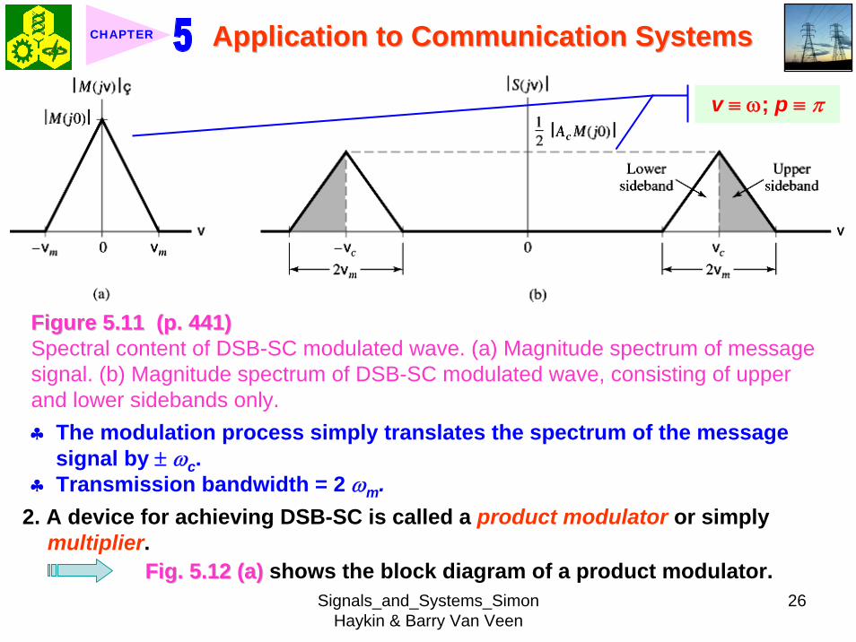
Signals_and_Systems_Simon Haykin amp Barry Van Veen
26
Application to Communication SystemsApplication to Communication SystemsCHAPTER
Figure 511 (p 441)Figure 511 (p 441)Spectral content of DSB-SC modulated wave (a) Magnitude spectrum of message signal (b) Magnitude spectrum of DSB-SC modulated wave consisting of upper and lower sidebands only
v equiv ω p equiv π
clubs The modulation process simply translates the spectrum of the message signal by plusmn ωc
clubs Transmission bandwidth = 2 ωm2 A device for achieving DSB-SC is called a product modulator or simply
multiplierFig 512 (a)Fig 512 (a) shows the block diagram of a product modulator
Signals_and_Systems_Simon Haykin amp Barry Van Veen
27
Application to Communication SystemsApplication to Communication SystemsCHAPTER
Figure 512 (p 441)Figure 512 (p 441)(a) Product modulator for generating the DSB-SC modulated wave (b) Coherent detector for demodulation of the DSB-SC modulated wave
v equiv ω p equiv π
552 552 Coherent DetectionCoherent Detection1 The message signal m(t) may be recovered from DSB-SC
Fig 512 (b)Fig 512 (b)ss((tt) ) timestimes locally generated sinusoidal wave = locally generated sinusoidal wave = vv((tt))vv((tt) filtered by a Low) filtered by a Low--pass filterpass filter
Local oscillator
2 The local oscillator should be exactly coherent or synchronized in both frequency and phase with the carrier wave c(t)
Signals_and_Systems_Simon Haykin amp Barry Van Veen
28
Application to Communication SystemsApplication to Communication SystemsCHAPTER
Coherent detection or synchronization demodulation3 Derivation for coherent detection
1) Local oscillator cos(ωct + φ )2) Product modulator output
( ) cos( ) ( )cos( ) cos( ) ( )
1 1cos( ) ( ) cos(2 ) ( )2 2
c
c c c
c c c
v t t s tA t t m t
A m t A t m t
ω φω ω φ
φ ω φ
= += +
= + +(519)
1 cos( ) ( )2 cA m tφ
1 cos(2 ) ( )2 c cA t m tω φ+
A scaled version of the original message signal m(t)
DSBDSB--SC modulated signal with carrier SC modulated signal with carrier frequency 2 frequency 2 ωωcc
3) Magnitude spectrum Fig 5134) To clear separate two component of v(t) the original carrier frequency ωc
must satisfy the condition
Signals_and_Systems_Simon Haykin amp Barry Van Veen
29
Application to Communication SystemsApplication to Communication SystemsCHAPTER
Figure 513 (p 442)Figure 513 (p 442)Magnitude spectrum of the product modulator output v(t) in the coherent detector of Fig 512(b)
v equiv ω p equiv π
2 c m mω ω ωminus gt c mω ωgt (520) ωωmm equivequiv message bandwidthmessage bandwidth
4 Specification of low-pass filter1) 1) The cutoff frequency must be The cutoff frequency must be ωωm m 2) The transition band must be 2) The transition band must be ωωm m ≦≦ ωω ≦≦ ωωc c ωωm m
Thus the overall output in Thus the overall output in Fig 512(b)Fig 512(b) is given byis given by1( ) cos( ) ( )2o cv t A m tφ= (521)
cosφ equiv attenuation factor
Signals_and_Systems_Simon Haykin amp Barry Van Veen
30
Application to Communication SystemsApplication to Communication SystemsCHAPTER
5 (1) Demodulated signal vo(t) is proportional to m(t) when the error phase φis a constant
(2) Demodulated signal is maximum when φ = 0 and has a minimum zero when φ = plusmn π2
Example 53 Sinusoidal DSB-SC ModulationConsider again the sinusoidal modulating signal
0 0( ) cos( )m t A tω=
( ) cos( )c cc t A tω=with amplitude A0 and frequency ω0 see Fig 514(a) The carrier wave is
with amplitude Ac and frequency ωc see Fig 514(b) Investigate the time-domain and frequency-domain characteristics of the corresponding DSB-SC modulated waveltltSolgtSolgt
clubs φ = plusmn π2 represents the quadrature null effect of the coherent detector
1 The modulated DSB-SC signal is defined by
0 0
0 0 0 0
( ) cos( ) cos( )1 1cos[( ) ] cos[( ) ]2 2
c c
c c c c
s t A A t t
A A t A A t
ω ω
ω ω ω ω
=
= + + minus
Signals_and_Systems_Simon Haykin amp Barry Van Veen
31
Application to Communication SystemsApplication to Communication SystemsCHAPTER
2 The Fourier transform of s(t) is given by
0 0 0
0 0
1( ) cos[ ( ) ( )]2
( ) ( )
c c c
c c
S j A Aω π δ ω ω ω δ ω ω ω
δ ω ω ω δ ω ω ω
= minus minus + + +
+ minus + + + minus
which consists of four weighted impulse functions at the frequencies ωc+ ω0-ωc- ω0 ωc- ω0 and- ωc+ ω0 as illustrated in the right-hand side of Fig Fig 514(c)514(c)
3 This Fourier transform differs from that depicted in the right-hand side of Fig Fig 56(c)56(c) for the corresponding example of full AM in one important respect The impulse functions at plusmn ωc due to the carrier are removed
4 Application of the sinusoidally modulated DSB-SC signal to the product modulator of Fig 512(b) yields the output (assuming φ = 0)
0 0 0
0 0 0 0 0
1( ) cos( ) cos[( ) ] cos[( ) ]21 cos[(2 ) ] cos( ) cos[(2 ) ] cos( )4
c c c c
c c c
v t A A t t t
A A t t t t
ω ω ω ω ω
ω ω ω ω ω ω
= + + minus
= + + + minus +
Signals_and_Systems_Simon Haykin amp Barry Van Veen
32
Application to Communication SystemsApplication to Communication SystemsCHAPTER
Figure 514 (p Figure 514 (p 443)443)Time-domain (on the left) and frequency-domain (on the right) characteristics of DSB-SC modulation produced by a sinusoidal modulating wave (a) Modulating wave (b) Carrier wave (c) DSB-SC modulated wave Note that ω= 2πƒ
v equiv ω p equiv π
Signals_and_Systems_Simon Haykin amp Barry Van Veen
33
Application to Communication SystemsApplication to Communication SystemsCHAPTER
5 The first two sinusoidal terms of v(t) are produced by the upper side frequency and the last two sinusoidal terms are produced by the lower side frequency
6 With ωcgt ω0 the first and third sinusoidal terms of frequencies 2ωc+ ω0 and 2ωc-ω0 respectively are removed by the low-pass filter of Fig 512(b)Fig 512(b) which leaves the second and fourth sinusoidal terms of frequency ω0 as the only output of the filter The coherent detector output thus reproduces the original modulating wave
7 Note however that this output appears as two equal terms one derived from the upper side frequency and the other from the lower side frequency We therefore conclude that for the transmission of the sinusoidal signal A0 cos(ω0t) only one side frequency is necessary (The issue will be discussed further in Section 57Section 57)
553 553 CostasCostas ReceiverReceiver1 Costas receiver Fig 515Fig 5152 This receiver consists of two coherent detector supplied with the same input
ie the incoming DSB-Sc wave
cos(2 ) ( )c cA f t m tπ but with individual local oscillator signals that are in phase duadrature with respect to each other
In-phase coherent detector (I-Channel) and quadrature-phase coherent detector (Q-Channel)
Signals_and_Systems_Simon Haykin amp Barry Van Veen
34
Application to Communication SystemsApplication to Communication SystemsCHAPTER
Figure 515 (p 445)Figure 515 (p 445)Costas receiver
v equiv ω p equiv π
Signals_and_Systems_Simon Haykin amp Barry Van Veen
35
Application to Communication SystemsApplication to Communication SystemsCHAPTER
56 56 QuadratureQuadrature--Carrier MultiplexingCarrier Multiplexing
Figure 516 (p 446)Figure 516 (p 446)Quadrature-carrier multiplexing system exploiting the quadrature null effect (a) Transmitter (b) Receiver assuming perfect synchronization with the transmitter
v equiv ω p equiv π
1 1 A A quadraturequadrature--carrier multiplexing or carrier multiplexing or quadraturequadrature--amplitude modulation (QAM) amplitude modulation (QAM) system enables two DSBsystem enables two DSB--SC modulated waves to occupy the same transmission SC modulated waves to occupy the same transmission bandwidth and yet it allows for their separation at the receivebandwidth and yet it allows for their separation at the receiver outputr output
BandwidthBandwidth--conservation schemeconservation scheme
Signals_and_Systems_Simon Haykin amp Barry Van Veen
36
Application to Communication SystemsApplication to Communication SystemsCHAPTER
2 Fig 5-16(a) Block diagram of the quadrature-carrier multiplexing systemFig 5-16(a) transmitter Fig 5-16(b) receiver
3 Multiplexed signal s(t)
(522) 1 2( ) ( ) cos( ) ( )sin( )c c c cs t A m t t A m t tω ω= +
where m1(t) and m2(t) denotes the two different message signals applied to the product modulations
clubsTransmission bandwidth = 2 ωm centered at ωc where ωm is the commonmessage bandwidth of m1(t) and m2(t)
4 The output of the top detector at receiver is 1
12 ( )cA m t
The output of the bottom detector at receiver is1
22 ( )cA m t
57 57 Other Variants of Amplitude Modulation Other Variants of Amplitude Modulation clubs Basic concept Full AM and DSB-SC rArr Wasteful of bandwidthclubs Given the amplitude and phase spectra of either lower or upper sideband
we can uniquely determine the other
Signals_and_Systems_Simon Haykin amp Barry Van Veen
37
Application to Communication SystemsApplication to Communication SystemsCHAPTER
clubs Single-sideband (SSB) modulation only one sideband is transmitted571 571 FrequencyFrequency--Domain Description of SSB ModulationDomain Description of SSB Modulation1 Consider a message signal m(t) with a spectrum M(jω) limited to the band
ωa le ω le ωb Fig 5-17 (a)2 DSB-SC modulated signal
( ) cos( )c cm t A tωtimes Fig 5-17 (b)
3 (1) Upper sideband the frequencies above ωc and below minus ωc(2) Upper sideband the frequencies below ωc and above minus ωc
Fig 5-17 (c)4 When only the lower sideband is transmitted the spectrum of the
corresponding SSB modulated wave is as shown in Fig 5-17 (d) 5 Advantages of SSB
(1) Reduced bandwidth requirement(2) Elimination of the high-power carrier waveDisadvantage od SSB(1) Cost and complexity of implementing both the transmitter and receiver
Signals_and_Systems_Simon Haykin amp Barry Van Veen
38
Application to Communication SystemsApplication to Communication SystemsCHAPTER
Figure 517 Figure 517 (p 447)(p 447)Frequency-domain characteristics of SSB modulation (a) Magnitude spectrum of message signal with energy gap from ndash ωa to ωa
(c) Magnitude spectrum of SSB modulated wave containing upper sideband only
(d) Magnitude spectrum of SSB modulated wave containing lower sideband only
(b) Magnitude spectrum of DSB-SC signal
v equiv ω p equiv π
Signals_and_Systems_Simon Haykin amp Barry Van Veen
39
Application to Communication SystemsApplication to Communication SystemsCHAPTER
6 Frequency-discrimination scheme for producing SSB modulation Fig 518clubs Bandpass filter is designed to pass the sideband selected for transmission
and suppress the remaining sidebandclubs Requirement in SSB signal the message signal applied to the product
modulator must have a energy gap in its spectrum Refer to Fig 517 (a)
Figure 518 (p 448)Figure 518 (p 448)System consisting of product modulator and bandpass filter for generating SSB modulated wave
v equiv ω p equiv π
572 572 TimeTime--Domain Description of SSB ModulationDomain Description of SSB Modulation1 Mathematical tool Hilbert transform
The Hilbert transform of a signal x(t) is defined by1 ( ) 1ˆ( ) ( )xx t d x t
t tτ τ
π τ πinfin
minusinfin= = lowast
minusint
Signals_and_Systems_Simon Haykin amp Barry Van Veen
40
Application to Communication SystemsApplication to Communication SystemsCHAPTER
The Fourier transform of 1(πt) is minus j times the signum function denoted
1 for 0sgn( ) 0 for 0
1 for 0
ωω ω
ω
+ gt⎧⎪= =⎨⎪minus lt⎩
2 Passing x(t) through a Hilbert transformer is equivalent to the combination of the following two operations in frequency domain1) Keeping X(jω)unchanged for all ω 2) Shifting areX(jω) (ie the phase spectrum of x(t)) by +90deg for negative
frequencies and minus 90deg for positive frequencies clubs Hilbert transformer = Wideband minus 90deg phase shifter 573 573 Vestigial Sideband ModulationVestigial Sideband Modulation1 When the message signal contains significant components at extremely
low frequencies the upper and lower sidebands meet at the carrier frequency
Using SSB is inappropriateUsing SSB is inappropriateEx TV signals or
wideband dataUsing VSB (Vestigial sideband) modulation is appropriateUsing VSB (Vestigial sideband) modulation is appropriate
Signals_and_Systems_Simon Haykin amp Barry Van Veen
41
Application to Communication SystemsApplication to Communication SystemsCHAPTER
2 VSB is a compromise between SSB and DSB-SC forms of modulationIn VSB modulation one sideband is passes almost completely whereas just a trace or vestige of the other sideband is retained
3 Fig 519 illustrates a VSB modulated wave s(t) in relation to the message signal m(t)
v equiv ω p equiv π
Figure 519 (p 449)Figure 519 (p 449)Spectral content of VSB modulated wave (a) Magnitude spectrum of message signal (c) Magnitude spectrum of VSB modulated wave containing a vestige of the lower sideband
clubs The lower sideband is modified into the vestigial sideband4 Transmission bandwidth of VSB modulated wave T m vω ω ω= + (523)
where ωm is the message bandwidth and ωu is the width of the vestigial sideband
Signals_and_Systems_Simon Haykin amp Barry Van Veen
42
Application to Communication SystemsApplication to Communication SystemsCHAPTER
5 Generation of VSB modulated wave Fig 520
Figure 520 (p 450)Figure 520 (p 450)System consisting of product modulator and sideband shaping filter for generating VSB modulated wave
v equiv ω p equiv π
Passing a DSBPassing a DSB--SC modulated wave through a sidebandSC modulated wave through a sideband--shaping filtershaping filter6 The sideband-shaping filter is designed so that the original message
spectrum M(jω) is reproduced on the demodulation as a result of the superposition of two spectra
1) The positive-frequency part of S(jω) (ie the Fourier transform of the transmitted signal s(t)) shifted downward in frequency by ωc
2) The negative-frequency part of S(jω) shifted upward in frequency by ωc
Fig 521 A reflection of the vestige of the lower sideband makes up for the missing parts of the upper sideband
Signals_and_Systems_Simon Haykin amp Barry Van Veen
43
Application to Communication SystemsApplication to Communication SystemsCHAPTER
Figure 521 (p 450)Figure 521 (p 450)Superposition of the two spectra shown in parts (a) and (b) of the figure results in the original message spectrum (shown dashed) upon demodulation
58 58 PulsePulse--Amplitude Modulation Amplitude Modulation clubs Basic concept
Basic role in the operation of AM Frequency-shiftingBasic role in the operation of PAM Sampling
581 581 Sampling RevisitedSampling Revisited1 Sampling theorem
In view point of PAMIn view point of PAM
Signals_and_Systems_Simon Haykin amp Barry Van Veen
44
Application to Communication SystemsApplication to Communication SystemsCHAPTER
1) A band-limited signal of finite energy that has no radian frequency components higher than ωm is uniquely determined by the values of the signal at instants of time separated by π ωm seconds
2) A band-limited signal of finite energy that has no radian frequency components higher than ωm may be completely recovered from a knowledge of its samples taken at the rate of ωm π per seconds
clubs Part 1) rArr Be exploited in the transmitter of a PAM clubs Part 2) rArr Be exploited in the Receiver of a PAM2 To combat the effects of aliasing in practice we use two corrective measures1) Prior to sampling a low-pass antialiasing filter is used to attenuate those high-
frequency components of the signal which lie outside the band of interest2) The filtered signal is sampled at a rate slightly higher than the Nyquist rate3 Generation of a PAM signal Fig 522Fig 522Example 54 Telephonic CommunicationThe highest frequency component of a speech signal needed for telephonic communication is about 31 kHz Suggest a suitable value for the sampling rate ltltSolgtSolgt
Signals_and_Systems_Simon Haykin amp Barry Van Veen
45
Application to Communication SystemsApplication to Communication SystemsCHAPTER
Figure 522 (p 451)Figure 522 (p 451)System consisting of antialiasing filter and sample-and-hold circuit for converting a message signal into a flattopped PAM signal
1 The highest frequency component of 31 kHz corresponds to 362 10 radsmω π= times
Correspondingly the Nyquist rate is
62 kHzmωπ
=
2 A suitable value for the sampling rate-one slightly higher than the Nyquistrate-may be 8 kHz a rate that is the international standard for telephone speech signals
Signals_and_Systems_Simon Haykin amp Barry Van Veen
46
Application to Communication SystemsApplication to Communication SystemsCHAPTER
582 582 Mathematical Description of PAMMathematical Description of PAM1 The carrier wave used in PAM consists of a sequence of short pulses of
fixed duration in terms of which PAM is formally defined as followsPAM is a form of pulse modulation in which the amplitude of the PAM is a form of pulse modulation in which the amplitude of the pulsed carrier is pulsed carrier is varied in accordance with instantaneous sample values of the mesvaried in accordance with instantaneous sample values of the message signalsage signal the duration of the pulsed carrier is maintained constant throughout
Fig 523Fig 523
Figure 523 (p452) Figure 523 (p452) Waveform of flattopped PAM signal with pulse duration T0 and sampling period Ts
Signals_and_Systems_Simon Haykin amp Barry Van Veen
47
Application to Communication SystemsApplication to Communication SystemsCHAPTER
2 Mathematical representation of the PAM
( ) [ ] ( )sn
s t m n b t nTinfin
=minusinfin
= minussum (524) s(t) equiv PAM signal m(t) equiv
message signal
Ts equiv sampling period m[n] equiv the values of m(t) at t = nTs h(t) equiv rectangular pulse of the unit amplitude and duration T0
3 Rectangular pulse
01 0( )
0 otherwiset T
h tlt lt⎧
= ⎨⎩
(525) Fig 524 (a)Fig 524 (a)
clubs Eq (524) is a sample-and-hold operationAnalogous to zeroAnalogous to zero--orderorder--holdhold--
based reconstruction in Sec 46based reconstruction in Sec 46
差異差異hh((tt) ) 的的TTss與與TT00
4 Impulse-sampled version of message signal m(t)
( ) [ ] ( )sn
m t m n t nTδ δinfin
=minusinfin
= minussum (526)
5 PAM signal( ) [ ] ( )
( ) ( )
sn
s t m n b t nT
m t b tδ
infin
=minusinfin
= minus
=
sum(527)
Convolution of impulse-sampled version mδ(t) and h(t)
Time domain Time domain operationoperation
Signals_and_Systems_Simon Haykin amp Barry Van Veen
48
Application to Communication SystemsApplication to Communication SystemsCHAPTER
Figure 524 (p 453)(a) Rectangular pulse h(t) of unit amplitude and duration T0 (b) Magnitude spectrum |H(jω)| and phase spectrum argH(jω) of pulse h(t)
v equiv ω p equiv π
Signals_and_Systems_Simon Haykin amp Barry Van Veen
49
Application to Communication SystemsApplication to Communication SystemsCHAPTER
6 FT of PAM signal( ) ( ) ( )S j M j H jδω ω ω= (528)
where( ) ( )FTS j s tω larr⎯rarr ( ) ( )FTM j m tδ δω larr⎯rarr ( ) ( )FTH j h tω larr⎯rarr
7 Impulse sampling of the message signal m(t) introduces periodicity into the spectrum as given by
1( ) ( ( ))sks
M j M j kTδ ω ω ω
infin
=minusinfin
= minussum (529) 1Ts equiv sampling rate ωs = 2πTs rads
1( ) ( ( )) ( )sks
S j M j k H jT
ω ω ω ωinfin
=minusinfin
= minussum (530)
( ) ( )FTM j m tω larr⎯rarrwhere
clubs Suppose that m(t) is strictly band limited and that the sampling rate 1Ts is greater than the Nyquist rate Then passing s(t) through a reconstruction filter chosen as an ideal low-pass filter with cutoff frequency ωm and gain Ts we find that the spectrum of the resulting filter output is equal to M(jω)H(jω)
Signals_and_Systems_Simon Haykin amp Barry Van Veen
50
Application to Communication SystemsApplication to Communication SystemsCHAPTER
8 From Eq (525) we find that0 2
0 0( ) sin ( (2 )) j TH j T c T e ωω ω π minus= (531) Fig 524(b) magnitude and phase of H(jω)
clubs Using PAM to represent a continuous-time message signal we introduce amplitude distortion as well as a delay of T02
clubs The frequency distortion caused by the use of flat-topped sampled in the generation of a PAM wave illustrated in Fig 523Fig 523 is referred to as the aperture effect
583 583 Demodulation of PAM SignalDemodulation of PAM Signal1 Reconstruction scheme Fig 525Fig 525
Figure 525 (p 454)Figure 525 (p 454)System consisting of low-pass interpolation filter and equalizer for reconstructing a message signal from its flattopped sampled version
clubs The system consists of low-pass interpolation filter and equalizer connected in cascade
Signals_and_Systems_Simon Haykin amp Barry Van Veen
51
Application to Communication SystemsApplication to Communication SystemsCHAPTER
2 The cutoff frequency of low-pass filter = the highest frequency ωm of message signal
3 The equalizer is used to correct the aperture effect due to flat-topped sampling in the sample-and-hold circuit
4 The equalizer has the effect of decreasing the in-band loss of the interpolation filter as frequency increases in such a manner as to compensate for the aperture effect
5 Amplitude response of equalizer
0
0 0 0 0
1 1 1| ( ) | | sinc( 2) | 2 | sin( 2) |
TH j T T T T
ωω ω ω
= =
Frequency response Eq (531)
Example 55 Equalization for PAM TransmissionThe duty cycle in a PAM signal namely T0 Ts is 10 Evaluate the peak amplification required for equalizationltltSolgtSolgt1 At ωm = π Ts which corresponds to the highest frequency component of the
message signal for a sampling rate equal to the Nyquist rate we find from Eq (531) that the magnitude response of the equalizer at ωm normalized to that at zero frequency is
Signals_and_Systems_Simon Haykin amp Barry Van Veen
52
Application to Communication SystemsApplication to Communication SystemsCHAPTER
Figure 526 (p 455)Figure 526 (p 455)Normalized equalization (to compensate for aperture effect) plotted against the duty cycle T0Ts
Signals_and_Systems_Simon Haykin amp Barry Van Veen
53
Application to Communication SystemsApplication to Communication SystemsCHAPTER
0
0 0
( 2)( )1sin (05 ) sin[( 2)( )]
s
s s
T Tc T T T T
ππ
=
where the ratio T0 Ts is equal to the duty cycle of the sampling pulses 2 In Fig 526Fig 526 this result is plotted as a function of the duty cycle T0 Ts Ideally it
should be equal to unity for all values of T0 Ts 3 For a duty cycle of 10 it is equal to 10041 It follows that for duty cycles of less
than 10 the magnitude equalization required is less than 10041 in which case the aperture effect is usually considered to be negligible
59 59 Multiplexing Multiplexing clubs Three basic types of multiplexing1 Frequency-division multiplexing in which the signals are separated by
allocating them to different frequency bands This is illustrated in Fig 527(a) for the case of six different message signals Frequency-division multiplexing favors the use of CW modulation where each message signal is able to use the channel on a continuous-time basis
2 Time-division multiplexing wherein the signals are separated by allocating them to different time slots within a sampling interval
Signals_and_Systems_Simon Haykin amp Barry Van Veen
54
Application to Communication SystemsApplication to Communication SystemsCHAPTER
This second type of multiplexing is illustrated in Fig 527(b) for the case of six different message signals Code-division multiplexing which relies on the assignment of different codes to the individual users of the channel
3 Code-division multiplexing which relies on the assignment of different codes to the individual users of the channel
591 591 FrequencyFrequency--Domain Multiplexing (FDM)Domain Multiplexing (FDM)1 Block diagram Fig 528Fig 5282 Incoming message signals low-pass variety3 Low-pass filter to remove high-frequency components such that the signal
in each channel does not disturb each other4 MOD (modulator) shift the frequency ranges of the signals so as to occupy
mutually exclusive frequency intervalsSSB is often used in this stageEx Voice input is usually assigned a bandwidth of 4 kHz
5 Band-pass filters are used to restrict the band of each modulated wave to its prescribed range
6 Band-pass filters in receiver separate the message signals7 DEM (demodulator) to recover signalsclubs FDM in Fig 528 operates in only one direction
Signals_and_Systems_Simon Haykin amp Barry Van Veen
55
Application to Communication SystemsApplication to Communication SystemsCHAPTER
Figure 527 (p 456)Figure 527 (p 456)Two basic forms of multiplexing (a) Frequency-division multiplexing (with guardbands) (b) Time-division multiplexing no provision is made here for synchronizing pulses
Signals_and_Systems_Simon Haykin amp Barry Van Veen
56
Application to Communication SystemsApplication to Communication SystemsCHAPTER
Figure 528 (p 457)Figure 528 (p 457)Block diagram of FDM system showing the important constituents of the transmitter and receiver
Signals_and_Systems_Simon Haykin amp Barry Van Veen
57
Application to Communication SystemsApplication to Communication SystemsCHAPTER
Example 56 SSB-FDM System
ltltSolgtSolgt
An FDM system is used to multiplex 24 independent voice signals SSB modulation is used for the transmission Given that each voice signal is allotted a bandwidth 4kHz calculate the overall transmission bandwidth of the channel
With each voice signal allotted a bandwidth of 4 kHz the use of SSB modulation requires a bandwidth of 4 kHz for its transmission Accordingly the overall transmission bandwidth provided by the channel is 24 X 4 = 96 kHz 592 592 TimeTime--Domain Multiplexing (TDM)Domain Multiplexing (TDM)clubs Basic to the operation of a TDM system is the sampling theoremclubs The transmission of the message samples engages the transmission channel for
only a fraction of the sampling interval on a periodic basis equal to the width T0 of a PAM modulating pulse
1 Block diagram Fig 529Fig 5292 Commutator is usually implemented by means of electronic switching
circuitry3 The function of commutator is two folds
Signals_and_Systems_Simon Haykin amp Barry Van Veen
58
Application to Communication SystemsApplication to Communication SystemsCHAPTER
Figure 529 (p 458)Figure 529 (p 458)Block diagram of TDM system showing the important constituents of the transmitter and receiver
(1) To take a narrow sample of each of the M input message signals at a rate 1Tsthat is slightly higher than ωcπ where ωc is the cutoff frequency of the input low-pass filter
(2) To sequentially interleave these M samples inside a sampling interval Ts4 Pulse modulator transform the multiplexed signal into a form suitable for
transmission over the common channel
Signals_and_Systems_Simon Haykin amp Barry Van Veen
59
Application to Communication SystemsApplication to Communication SystemsCHAPTER
clubs The use of time-division multiplexing introduces a bandwidth expansion factor M because the scheme must squeeze M samples derived from M independent message sources into a time slot equal to one sampling interval
5 Pulse demodulator performs the inverse operation of the pulse modulator6 Decommutator distributes the narrow samples produced by pulse demodulator to the appropriate low-pass reconstruction filter7 Synchronization between the timing operations of the transmitter and
receiver in a TDM system is essential for satisfactory performance of the system
Inserting an extra pulse into each sampling interval on a regular basisBandwidth expansion factor is increased to M + 1
clubs The TDM system is hghly sensitive to the dispersion in the common transmission channel
Example 57 Comparison of TDM with FDMATDM system is used to multiplex four independent voice signals using PAM Each voice signal is sampled at the rate of 8 kHz The system incorporates a synchronizing pulse train for its proper operation
Signals_and_Systems_Simon Haykin amp Barry Van Veen
60
Application to Communication SystemsApplication to Communication SystemsCHAPTER
(a) Determine the timing relationships between the synchronizing pulse train and the impulse trains used to sample the four voice signals
(b) Calculate the transmission bandwidth of the channel for the TDM system and compare the result with a corresponding FDM system using SSBmodulation
ltltSolgtSolgt(a) The sampling period is
31 125 s
8 10sT s μ= =times
In this example the number of voice signals is M = 4 Hence dividing the sampling period of 125 μs among these voice signals and the synchronizing pulse train we obtain the time slot allocated to each one of them
0 1125 25 s
5
sTTM
μ
=+
= =
Signals_and_Systems_Simon Haykin amp Barry Van Veen
61
Application to Communication SystemsApplication to Communication SystemsCHAPTER
Figure 530Figure 530 shows the timing relationships between the synchronizing pulse train and the four impulse trains used to sample the different voice signals in a single frame Each frame includes time slots of common duration T0 = 25 μs which are allocated to the pulse-modulated signals and synchronizing pulse
Figure 530 (p 459)Figure 530 (p 459)Composition of one frame of a multiplexed PAM signal incorporating four voice-signals and a synchronizing pulse
Signals_and_Systems_Simon Haykin amp Barry Van Veen
62
Application to Communication SystemsApplication to Communication SystemsCHAPTER
(b) As a consequence of the time-bandwidth product (see Section 317) there is an inverse relationship between the duration of a pulse and the bandwidth (ie cutoff frequency) of the channel needed for itstransmission Accordingly the overall transmission bandwidth of the channel is
0
21 1 MHz 40 kHz
25
TTf
T
ωπ
=
= = =
In contrast the use of an FDM system based on SSB modulation requires a channel bandwidth equal to M times that of a single voice signal-that is 4 X 4 = 16 kHz Thus the use of PAM-TDM requires a channel bandwidth that is 40 16 = 25 times that of SSB-FDMIn practice pulse-code modulation is commonly used as the method of modulation for TDM this results in a further increase in channel bandwidth depending on the length of the code word used in the digital representation of each pulse in the PAM signal
Signals_and_Systems_Simon Haykin amp Barry Van Veen
63
Application to Communication SystemsApplication to Communication SystemsCHAPTER
510 510 Pulse and Group Delays Pulse and Group Delays 1 Whenever a signal is transmitted through a dispersive (ie frequency
selective) system some delay is introduced into the output signal in relation to the input signal
2 The delay is determined by the phase response of the system3 Phase response of a dispersive communication channel
( ) arg ( )H jφ ω ω= (532)
A signal is transmitted through the channel at a frequency ωc The signal received at the channel lags the transmitted signal by φ(ωc) The time delay is called phase delay formally defined as
( )cp
c
φ ωτω
= minus (533)
The phase delay is not necessarily the true signal delayclubs Case study for DSB-SC1 Transmitted signal
0( ) cos( ) cos( )cs t A t tω ω= (534)
ωc equiv carrier frequency ω0 equiv sinusoidal modulation frequency
A = AcA0
Signals_and_Systems_Simon Haykin amp Barry Van Veen
64
Application to Communication SystemsApplication to Communication SystemsCHAPTER
1 21 1( ) cos( ) cos( )2 2
s t A t A tω ω= +
1 0cω ω ω= + (535) where
2 0cω ω ω= minus (536)
Upper frequency
Lower frequency
2 Let the s(t) be transmitted through the channel with phase response φ (ω) Accordingly the signal received at the channel output is
1 1 2 21 1( ) cos( ( )) cos( ( ))2 2
y t A t A tω φ ω ω φ ω= + + +
1 2 1 20
( ) ( ) ( )1 ( )( ) cos cos2 2cy t A t tφ ω φ ω φ ω φ ωω ω+⎛ ⎞ ⎛ ⎞= + +⎜ ⎟ ⎜ ⎟
⎝ ⎠ ⎝ ⎠(537)
3 Two observations from Eq (537)1) The carrier component at frequency ωc in y(t) lags its counterpart in s(t) by
frac12 (φ (ω1) + φ (ω2)) which represents a time delay equal to
1 2 1 2
c 1 2
( )+ ( ) ( )+ ( )2 +
φ ω φ ω φ ω φ ωω ω ω
minus = minus (538)
Signals_and_Systems_Simon Haykin amp Barry Van Veen
65
Application to Communication SystemsApplication to Communication SystemsCHAPTER
2) The message component at frequency ω0 in y(t) lags its counterpart in s(t) by frac12 (φ (ω1) minus φ (ω2)) which represents a time delay equal to
1 2 1 2
0 1 2
( ) ( ) ( ) ( )2
φ ω φ ω φ ω φ ωω ω ωminus minus
minus = minusminus
(539)
4 Suppose that ω0 lt ωc rArr the side frequencies are close together with ω c between them Such a modulated signal is said to be a narrowband signal The phase response φ (ω) in the vicinity of ω = ωc is approximated by two-term Taylor series expansion
( )( ) ( ) ( )c
c cd
d ω ω
φ ωφ ω φ ω ω ωω =
= + times minus (540)
Phase delay = ( ) c cφ ω ωminus
5 The time delay introduced by the message signal (ie he ldquoenveloperdquo of the modulated signal) is given by
( )
c
gd
d ω ω
φ ωτω =
= minus (541) The time delay τg is called the
envelope delay or group delay
Signals_and_Systems_Simon Haykin amp Barry Van Veen
66
Application to Communication SystemsApplication to Communication SystemsCHAPTER
6 When a modulated signal is transmitted through a communication channel there are two different delays to be considered1) The carrier or phase delay τp defined by Eq (533)2) The envelope or group delay τg defined by Eq (541)
clubs The group delay is the true signal delay
Example 58 Phase and Group Delays for Ban-pass Channel
ltltSolgtSolgt
The phase response of a band-pass communication channel is defined by 2 2
1( ) tan c
c
ω ωφ ωωω
minus ⎛ ⎞minus= minus ⎜ ⎟
⎝ ⎠The signal s(t) defined in Eq (534) is transmitted through this channel with
475 radscω = 0 025 radsω =andCalculate (a) the phase delay and (b) the group delay
(a) At ω = ωc φ (ωc) = 0 According to Eq (533) the phase delay τ p is zero (b) Differentiating φ (ω) with respect to ω we get
Signals_and_Systems_Simon Haykin amp Barry Van Veen
67
Application to Communication SystemsApplication to Communication SystemsCHAPTER
2 2
2 2 2 2 2
( )( )( )
c c
c c
dd
ω ω ωφ ωω ω ω ω ω
+= minus
+ minus
Using thing result in Eq (541) we find that the group delay is 2 2 04211
475gc
sτω
= = =
1 One waveform shown as a solid curve was obtained by multiplying the transmitted signal s(t) by the carrier wave cos(ωct)
2 The second waveform shown as a dotted curve was obtained by multiplying the received signal y(t) by the carrier wave cos(ωct)
To display the results obtained in parts (a) and (b) in graphical form Fig 531Fig 531shows a superposition of two waveforms obtained as follows
The figure clearly shows that the carrier (phase) delay τ p is zero and the envelope of the received signal y(t) is lagging behind that of the transmitted signal by τs seconds For the presentation of waveforms in this figure we purposely did not use a filter to suppress the high frequency components resulting from the multiplications described under points 1 and 2 because of the desire to retain a contribution due to the carrier for display
Signals_and_Systems_Simon Haykin amp Barry Van Veen
68
Application to Communication SystemsApplication to Communication SystemsCHAPTER
Figure 531 Figure 531 (p 463)(p 463)Highlighting the zero carrier delay (solid curve) and group delay τg (dotted curve) which are determined in accordance with Example 58
Signals_and_Systems_Simon Haykin amp Barry Van Veen
69
Application to Communication SystemsApplication to Communication SystemsCHAPTER
clubs Not also that the separation between the upper side frequency ω1 = ωc + ω0 = 500 rads and the lower side frequency ω2 = ωc minus ω0 = 450 rads is about 10 of the carrier frequency ωc = 475 rads which justifies referring to the modulated signal in this example as a narrowband signal
5101 5101 Some Practical ConsiderationsSome Practical Considerationsclubs What is the practical importance of group delay 1 Eq (541) for determining group delay applies strictly to narrowband
modulated signal2 The message bandwidth may be comparable to the carrier frequency In
this situation the group delay is formulated as a frequency-dependent parameter ie ( )d( )g d
φ ωτ ωω
= minus (542)
3 When a wideband modulated signals transmitted through a dispersive channel the frequency components of the message signal are delayed by different amounts at the channel output
Delay distortionFig 532Fig 532 Group delay response of voice-grade telephone channel
Signals_and_Systems_Simon Haykin amp Barry Van Veen
70
Application to Communication SystemsApplication to Communication SystemsCHAPTER
Figure 532 (p 464)Group delay response of voice-grade telephone channel (Adapted from J C Bellamy Digital Telephony Wiley 1982)
511 511 Exploring Concepts with MATLABExploring Concepts with MATLAB5111 5111 Full AMFull AMclubs Sinusoidal modulation
clubs To reconstruct a faithful version of the original message signal in the receiver we have to use a delay equalizer
0( ) [1 cos( )]cos( )c cs t A t tμ ω ω= +1 AM experiment
1cA =
08 radscω π= 0 01 radsω π=Carrier amplitude
Carrier frequency Modulation amplitude
Signals_and_Systems_Simon Haykin amp Barry Van Veen
71
Application to Communication SystemsApplication to Communication SystemsCHAPTER
2 We wish to display and analyze 10 full cycles of the AM wave corresponding to a total duration of 200 s Choosing a sampling rate 1Ts = 10 Hz we have a total of N = 2000 time samples The frequency band of interest is minus 10 π ≦ ω ≦ 10 π Since the separation between the carrier and either side frequency is equal to the modulation frequency ω0 = 01 π rads we would like to have a frequency resolution ωr = 001π rads To achieve this resolution we require the following number of frequency samples (see Eq (442))
20 2000001
s
r
M ω πω π
ge = =
3 We therefore choose M = 2000 To approximate the Fourier transform of the AM wave s(t) we may use a 2000-point DTFS The only variable in the AM experiment is the modulation factor μ with respect to which we wish to investigate three different situationsμ = 05 corresponding to under-modulationμ = 10 for which the AM system is on the verge of over-modulationμ = 20 corresponding to over-modulation
Signals_and_Systems_Simon Haykin amp Barry Van Veen
72
Application to Communication SystemsApplication to Communication SystemsCHAPTER
4 MATLAB commandsAc = 1 carrier amplitudewc = 08pi carrier frequencyw0 = 01pi modulation frequencymu = 05 modulation factort = 0011999s = Ac(1 + mucos(w0t))cos(wct)plot(ts)Smag = abs(fftshift(fft(s2000)))2000 Smag denotes the magnitude specturm of the AM wavew = 10[-1000999]2pi2000plot(wSmag)axis ([-30 30 0 08])
5 5 μμ = 05 = 05 case case Fig 533Fig 533μμ = 10 case = 10 case Fig 534Fig 534μμ = 20 case = 20 case Fig 535Fig 535
Discussion see pp 466-469 textbook
Signals_and_Systems_Simon Haykin amp Barry Van Veen
73
Application to Communication SystemsApplication to Communication SystemsCHAPTER
-30 -20 -10 0 10 20 300
02
04
06
0 50 100 150 200-2
-1
0
1
2
2 22 24 26 28 3
02
04
06
(a) Time (s)
Time domain
Frequency domain
(b) Frequency (rads)
Frequency domain
Frequency (rads)
Figure 533 (p 466)Amplitude modulation with 50 modulation (a) AM wave (b) magnitude spectrum of the AM wave and (c) expanded spectrum around the carrier frequency
μμ = 05 = 05 casecase
Signals_and_Systems_Simon Haykin amp Barry Van Veen
74
Application to Communication SystemsApplication to Communication SystemsCHAPTER
Figure 534 (p 467)Figure 534 (p 467)Amplitude modulation with 100 modulation (a) AM wave (b) magnitude spectrum of the AM wave and (c) expanded spectrum around the carrier frequency
Signals_and_Systems_Simon Haykin amp Barry Van Veen
75
Application to Communication SystemsApplication to Communication SystemsCHAPTER
Figure 535 (p 468)Amplitude modulation with 200 modulation (a) AM wave (b) magnitude spectrum of the AM wave and (c) expanded spectrum around the carrier frequency
Signals_and_Systems_Simon Haykin amp Barry Van Veen
76
Application to Communication SystemsApplication to Communication SystemsCHAPTER
5112 5112 DSBDSB--SC ModulationSC Modulation1 Sinusoidal modulation
0 0( ) cos( ) cos( )c cs t A A t tω ω=
2 MATLAB commands
Ac = 1 carrier amplitudewc = 08pi carrier frequency in radsA0 = 1 amplitude of modulating signalw0 = 01pi frequency of modulating signalt = 011999s = AcA0cos(wct)cos(w0t)plot(ts)Smag = abs(fftshift(fft(s2000)))2000w = 10[-1000999]2pi2000plot(wSmag)
3 3 DSBDSB--SC modulated waveSC modulated wave Fig 536Fig 536 Discussion see pp 466-469 textbook
4 Output of the product modulator in Fig 512 (b) with φ = 0
Signals_and_Systems_Simon Haykin amp Barry Van Veen
77
Application to Communication SystemsApplication to Communication SystemsCHAPTER
Figure 536 (p 469)DSB-SC modulation (a) DSB-SC modulated wave (b) magnitude spectrum of the modulated wave and (c) expanded spectrum around the carrier frequency
Signals_and_Systems_Simon Haykin amp Barry Van Veen
78
Application to Communication SystemsApplication to Communication SystemsCHAPTER
( ) ( ) cos( )cv t s t tω=
5 MATLAB commandsgtgt v = scos(wct)
6 Fig 537 (a) waveforms of v(t) Fig 537 (b) magnitude spectrum which readily shows that v(t) consists of the following components1) A sinusoidal component with frequency 01π rads representing the
modulating wave2) A new DSB-SC modulated wave with double carrier frequency of 16π rads
in actuality the side frequencies of this modulated wave are located at 15πand 17π rads
1) The frequency of the modulating wave lies inside the passband of the filter2) The upper and lower side frequencies of the new DSB-SC modulated wave
lie inside the stopband of the filter
Accordingly we may recover the sinusoidal modulating signal by passing v(t) through low-pass filter with the following requirements
Signals_and_Systems_Simon Haykin amp Barry Van Veen
79
Application to Communication SystemsApplication to Communication SystemsCHAPTER
Figure 537 (p 470)Coherent detection of DSB-SC modulated wave (a) and (b) Waveform and magnitude spectrum of signal produced at the output of produce modulator (c) and (d) waveform and magnitude spectrum of low-pass filter output
Signals_and_Systems_Simon Haykin amp Barry Van Veen
80
Application to Communication SystemsApplication to Communication SystemsCHAPTER
The issue of how to design a filter with these requirements will be considered in detail in Chapter 8 For the present it suffices to say that the preceding requirements can be met by using the following MATLAB commands
gtgt [ba] = butter(30025)gtgt output = filter(bav)
The first command produces s special type of filter called a Butterworth filter For the experiment considered here the filter order is 3 and its normalized cutoff frequency of 0025 is calculated as follows
Actual cutoff frequency of filter 025 radsHalf the sampling rate 10 rads
0025
ππ
=
=
The second command computes the filterrsquos output in response to the product modulator output v(t) (We will revisit the design of this filter in Chapter 8) Figure 537(c) displays the waveform of the low-pass filter output this waveform represents a sinusoidal signal of frequency 005 Hz an observation that is confirmed by using the ffr command to approximate the spectrum of the filter output The result of the computation is shown in Fig 537(d)Fig 537(d)
Signals_and_Systems_Simon Haykin amp Barry Van Veen
81
Application to Communication SystemsApplication to Communication SystemsCHAPTER
7 In Fig 538 we explore another aspect of DSB-SC modulation namely the effect of varying the modulation frequency Figure 538(a) shows five cycles of a DSB-SC modulated wave that has the same carrier frequency as that in Fig 536(a) but the modulation frequency has been reduced to 0025 Hz( ie a radian frequency of 005π) Figure 538(b) shows the magnitude spectrum of this second DSB-SC modulated wave and its zoomed-in version is shown in Fig 538(c) Comparing this latter figure with Fig 536(c) we see clearly that decreasing the modulation frequency has the effect of moving the upper and lower side frequencies closer together which is consistent with modulation theory
5113 5113 Phase and Group DelayPhase and Group Delay1 In Example 58 we studied the phase and group delays for a band-pass
channel with phase response 2 2
1( ) tan c
c
ω ωφ ωωω
minus ⎛ ⎞minus= minus ⎜ ⎟
⎝ ⎠2 At ω = ωc the phase delay is τ p = 0 and the group delay is τ s = 04211s One
of the wave forms displayed in Fig 531Fig 531 is
1( ) ( ) cos( )cx t s t tω=
Signals_and_Systems_Simon Haykin amp Barry Van Veen
82
Application to Communication SystemsApplication to Communication SystemsCHAPTER
Figure 538 (p 472)Effect of varying the modulation frequency compared with that in Fig 537 (a) and (b) Waveform and magnitude spectrum of DSB-SC modulated wave with a modulation frequency one-half that used in Fig 536 (c) expanded spectrum around the carrier frequency
Signals_and_Systems_Simon Haykin amp Barry Van Veen
83
Application to Communication SystemsApplication to Communication SystemsCHAPTER
where (see page 461)
1 2( ) [cos( ) cos( )]2As t t tω ω= +
and ω1 = ωc + ω0 and ω2 = ωc - ω0 The waveform shown in the figure as a solid curve is a plot of x1(t) The other waveform also displayed in Fig 531Fig 531 is
2
1 1 2 2
( ) ( ) cos( )
[cos( ( )) cos( ( ))]cos( )2
c
c
x t y t tA t t t
ω
ω φ ω ω φ ω ω
=
= + + +
where the angle φ (ω1) and φ (ω2) are the values of the phase response φ (ω) at ω = ω1 and ω = ω2 respectively The waveform shown as a dotted curve in the figure is a plot of x2(t)
3 The generation of x1(t) and x2(t) in MATLAB is achieved with the following commands with A2 set equal to unity
Signals_and_Systems_Simon Haykin amp Barry Van Veen
84
Application to Communication SystemsApplication to Communication SystemsCHAPTER
wc = 475w0 = 025w1 = wc + w0w2 = wc - w0t = -10 0001 10o1 = -atan((w1^2 - wc^2)(w1wc))o2 = -atan((w2^2 - wc^2)(w2wc))s = cos(w1t) + cos(w2t)y = cos(w1t + o1) + cos(w2t + o2)x1 = scos(478t)x2 = ycos(475t)plot(tx1b)hold on plot(tx2k)hold offxlabel(Time)ylabel(Amplitude)
Note that we have set (A2) = 1 for convenience of presentation The function atan in the first two commands returns the arctangent Note also that the computation of both x1 and x2 involve element-by-element multiplications ndash hence the use of period followed by an asterisk
Signals_and_Systems_Simon Haykin amp Barry Van Veen
85
Application to Communication SystemsApplication to Communication SystemsCHAPTER
Signals_and_Systems_Simon Haykin amp Barry Van Veen
86
Application to Communication SystemsApplication to Communication SystemsCHAPTER
Signals_and_Systems_Simon Haykin amp Barry Van Veen
87
Application to Communication SystemsApplication to Communication SystemsCHAPTER
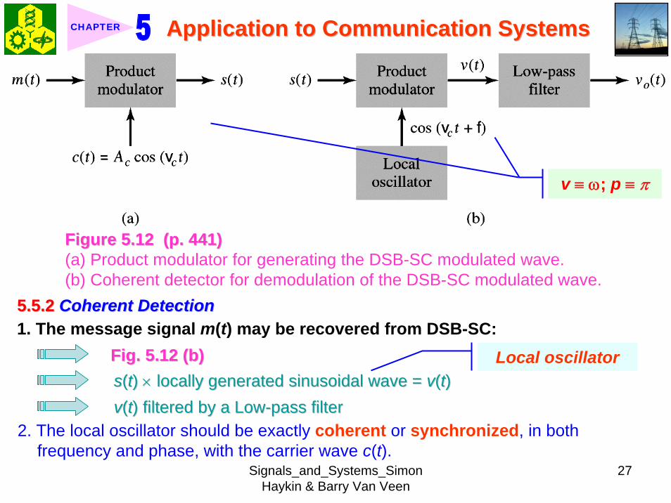
Signals_and_Systems_Simon Haykin amp Barry Van Veen
27
Application to Communication SystemsApplication to Communication SystemsCHAPTER
Figure 512 (p 441)Figure 512 (p 441)(a) Product modulator for generating the DSB-SC modulated wave (b) Coherent detector for demodulation of the DSB-SC modulated wave
v equiv ω p equiv π
552 552 Coherent DetectionCoherent Detection1 The message signal m(t) may be recovered from DSB-SC
Fig 512 (b)Fig 512 (b)ss((tt) ) timestimes locally generated sinusoidal wave = locally generated sinusoidal wave = vv((tt))vv((tt) filtered by a Low) filtered by a Low--pass filterpass filter
Local oscillator
2 The local oscillator should be exactly coherent or synchronized in both frequency and phase with the carrier wave c(t)
Signals_and_Systems_Simon Haykin amp Barry Van Veen
28
Application to Communication SystemsApplication to Communication SystemsCHAPTER
Coherent detection or synchronization demodulation3 Derivation for coherent detection
1) Local oscillator cos(ωct + φ )2) Product modulator output
( ) cos( ) ( )cos( ) cos( ) ( )
1 1cos( ) ( ) cos(2 ) ( )2 2
c
c c c
c c c
v t t s tA t t m t
A m t A t m t
ω φω ω φ
φ ω φ
= += +
= + +(519)
1 cos( ) ( )2 cA m tφ
1 cos(2 ) ( )2 c cA t m tω φ+
A scaled version of the original message signal m(t)
DSBDSB--SC modulated signal with carrier SC modulated signal with carrier frequency 2 frequency 2 ωωcc
3) Magnitude spectrum Fig 5134) To clear separate two component of v(t) the original carrier frequency ωc
must satisfy the condition
Signals_and_Systems_Simon Haykin amp Barry Van Veen
29
Application to Communication SystemsApplication to Communication SystemsCHAPTER
Figure 513 (p 442)Figure 513 (p 442)Magnitude spectrum of the product modulator output v(t) in the coherent detector of Fig 512(b)
v equiv ω p equiv π
2 c m mω ω ωminus gt c mω ωgt (520) ωωmm equivequiv message bandwidthmessage bandwidth
4 Specification of low-pass filter1) 1) The cutoff frequency must be The cutoff frequency must be ωωm m 2) The transition band must be 2) The transition band must be ωωm m ≦≦ ωω ≦≦ ωωc c ωωm m
Thus the overall output in Thus the overall output in Fig 512(b)Fig 512(b) is given byis given by1( ) cos( ) ( )2o cv t A m tφ= (521)
cosφ equiv attenuation factor
Signals_and_Systems_Simon Haykin amp Barry Van Veen
30
Application to Communication SystemsApplication to Communication SystemsCHAPTER
5 (1) Demodulated signal vo(t) is proportional to m(t) when the error phase φis a constant
(2) Demodulated signal is maximum when φ = 0 and has a minimum zero when φ = plusmn π2
Example 53 Sinusoidal DSB-SC ModulationConsider again the sinusoidal modulating signal
0 0( ) cos( )m t A tω=
( ) cos( )c cc t A tω=with amplitude A0 and frequency ω0 see Fig 514(a) The carrier wave is
with amplitude Ac and frequency ωc see Fig 514(b) Investigate the time-domain and frequency-domain characteristics of the corresponding DSB-SC modulated waveltltSolgtSolgt
clubs φ = plusmn π2 represents the quadrature null effect of the coherent detector
1 The modulated DSB-SC signal is defined by
0 0
0 0 0 0
( ) cos( ) cos( )1 1cos[( ) ] cos[( ) ]2 2
c c
c c c c
s t A A t t
A A t A A t
ω ω
ω ω ω ω
=
= + + minus
Signals_and_Systems_Simon Haykin amp Barry Van Veen
31
Application to Communication SystemsApplication to Communication SystemsCHAPTER
2 The Fourier transform of s(t) is given by
0 0 0
0 0
1( ) cos[ ( ) ( )]2
( ) ( )
c c c
c c
S j A Aω π δ ω ω ω δ ω ω ω
δ ω ω ω δ ω ω ω
= minus minus + + +
+ minus + + + minus
which consists of four weighted impulse functions at the frequencies ωc+ ω0-ωc- ω0 ωc- ω0 and- ωc+ ω0 as illustrated in the right-hand side of Fig Fig 514(c)514(c)
3 This Fourier transform differs from that depicted in the right-hand side of Fig Fig 56(c)56(c) for the corresponding example of full AM in one important respect The impulse functions at plusmn ωc due to the carrier are removed
4 Application of the sinusoidally modulated DSB-SC signal to the product modulator of Fig 512(b) yields the output (assuming φ = 0)
0 0 0
0 0 0 0 0
1( ) cos( ) cos[( ) ] cos[( ) ]21 cos[(2 ) ] cos( ) cos[(2 ) ] cos( )4
c c c c
c c c
v t A A t t t
A A t t t t
ω ω ω ω ω
ω ω ω ω ω ω
= + + minus
= + + + minus +
Signals_and_Systems_Simon Haykin amp Barry Van Veen
32
Application to Communication SystemsApplication to Communication SystemsCHAPTER
Figure 514 (p Figure 514 (p 443)443)Time-domain (on the left) and frequency-domain (on the right) characteristics of DSB-SC modulation produced by a sinusoidal modulating wave (a) Modulating wave (b) Carrier wave (c) DSB-SC modulated wave Note that ω= 2πƒ
v equiv ω p equiv π
Signals_and_Systems_Simon Haykin amp Barry Van Veen
33
Application to Communication SystemsApplication to Communication SystemsCHAPTER
5 The first two sinusoidal terms of v(t) are produced by the upper side frequency and the last two sinusoidal terms are produced by the lower side frequency
6 With ωcgt ω0 the first and third sinusoidal terms of frequencies 2ωc+ ω0 and 2ωc-ω0 respectively are removed by the low-pass filter of Fig 512(b)Fig 512(b) which leaves the second and fourth sinusoidal terms of frequency ω0 as the only output of the filter The coherent detector output thus reproduces the original modulating wave
7 Note however that this output appears as two equal terms one derived from the upper side frequency and the other from the lower side frequency We therefore conclude that for the transmission of the sinusoidal signal A0 cos(ω0t) only one side frequency is necessary (The issue will be discussed further in Section 57Section 57)
553 553 CostasCostas ReceiverReceiver1 Costas receiver Fig 515Fig 5152 This receiver consists of two coherent detector supplied with the same input
ie the incoming DSB-Sc wave
cos(2 ) ( )c cA f t m tπ but with individual local oscillator signals that are in phase duadrature with respect to each other
In-phase coherent detector (I-Channel) and quadrature-phase coherent detector (Q-Channel)
Signals_and_Systems_Simon Haykin amp Barry Van Veen
34
Application to Communication SystemsApplication to Communication SystemsCHAPTER
Figure 515 (p 445)Figure 515 (p 445)Costas receiver
v equiv ω p equiv π
Signals_and_Systems_Simon Haykin amp Barry Van Veen
35
Application to Communication SystemsApplication to Communication SystemsCHAPTER
56 56 QuadratureQuadrature--Carrier MultiplexingCarrier Multiplexing
Figure 516 (p 446)Figure 516 (p 446)Quadrature-carrier multiplexing system exploiting the quadrature null effect (a) Transmitter (b) Receiver assuming perfect synchronization with the transmitter
v equiv ω p equiv π
1 1 A A quadraturequadrature--carrier multiplexing or carrier multiplexing or quadraturequadrature--amplitude modulation (QAM) amplitude modulation (QAM) system enables two DSBsystem enables two DSB--SC modulated waves to occupy the same transmission SC modulated waves to occupy the same transmission bandwidth and yet it allows for their separation at the receivebandwidth and yet it allows for their separation at the receiver outputr output
BandwidthBandwidth--conservation schemeconservation scheme
Signals_and_Systems_Simon Haykin amp Barry Van Veen
36
Application to Communication SystemsApplication to Communication SystemsCHAPTER
2 Fig 5-16(a) Block diagram of the quadrature-carrier multiplexing systemFig 5-16(a) transmitter Fig 5-16(b) receiver
3 Multiplexed signal s(t)
(522) 1 2( ) ( ) cos( ) ( )sin( )c c c cs t A m t t A m t tω ω= +
where m1(t) and m2(t) denotes the two different message signals applied to the product modulations
clubsTransmission bandwidth = 2 ωm centered at ωc where ωm is the commonmessage bandwidth of m1(t) and m2(t)
4 The output of the top detector at receiver is 1
12 ( )cA m t
The output of the bottom detector at receiver is1
22 ( )cA m t
57 57 Other Variants of Amplitude Modulation Other Variants of Amplitude Modulation clubs Basic concept Full AM and DSB-SC rArr Wasteful of bandwidthclubs Given the amplitude and phase spectra of either lower or upper sideband
we can uniquely determine the other
Signals_and_Systems_Simon Haykin amp Barry Van Veen
37
Application to Communication SystemsApplication to Communication SystemsCHAPTER
clubs Single-sideband (SSB) modulation only one sideband is transmitted571 571 FrequencyFrequency--Domain Description of SSB ModulationDomain Description of SSB Modulation1 Consider a message signal m(t) with a spectrum M(jω) limited to the band
ωa le ω le ωb Fig 5-17 (a)2 DSB-SC modulated signal
( ) cos( )c cm t A tωtimes Fig 5-17 (b)
3 (1) Upper sideband the frequencies above ωc and below minus ωc(2) Upper sideband the frequencies below ωc and above minus ωc
Fig 5-17 (c)4 When only the lower sideband is transmitted the spectrum of the
corresponding SSB modulated wave is as shown in Fig 5-17 (d) 5 Advantages of SSB
(1) Reduced bandwidth requirement(2) Elimination of the high-power carrier waveDisadvantage od SSB(1) Cost and complexity of implementing both the transmitter and receiver
Signals_and_Systems_Simon Haykin amp Barry Van Veen
38
Application to Communication SystemsApplication to Communication SystemsCHAPTER
Figure 517 Figure 517 (p 447)(p 447)Frequency-domain characteristics of SSB modulation (a) Magnitude spectrum of message signal with energy gap from ndash ωa to ωa
(c) Magnitude spectrum of SSB modulated wave containing upper sideband only
(d) Magnitude spectrum of SSB modulated wave containing lower sideband only
(b) Magnitude spectrum of DSB-SC signal
v equiv ω p equiv π
Signals_and_Systems_Simon Haykin amp Barry Van Veen
39
Application to Communication SystemsApplication to Communication SystemsCHAPTER
6 Frequency-discrimination scheme for producing SSB modulation Fig 518clubs Bandpass filter is designed to pass the sideband selected for transmission
and suppress the remaining sidebandclubs Requirement in SSB signal the message signal applied to the product
modulator must have a energy gap in its spectrum Refer to Fig 517 (a)
Figure 518 (p 448)Figure 518 (p 448)System consisting of product modulator and bandpass filter for generating SSB modulated wave
v equiv ω p equiv π
572 572 TimeTime--Domain Description of SSB ModulationDomain Description of SSB Modulation1 Mathematical tool Hilbert transform
The Hilbert transform of a signal x(t) is defined by1 ( ) 1ˆ( ) ( )xx t d x t
t tτ τ
π τ πinfin
minusinfin= = lowast
minusint
Signals_and_Systems_Simon Haykin amp Barry Van Veen
40
Application to Communication SystemsApplication to Communication SystemsCHAPTER
The Fourier transform of 1(πt) is minus j times the signum function denoted
1 for 0sgn( ) 0 for 0
1 for 0
ωω ω
ω
+ gt⎧⎪= =⎨⎪minus lt⎩
2 Passing x(t) through a Hilbert transformer is equivalent to the combination of the following two operations in frequency domain1) Keeping X(jω)unchanged for all ω 2) Shifting areX(jω) (ie the phase spectrum of x(t)) by +90deg for negative
frequencies and minus 90deg for positive frequencies clubs Hilbert transformer = Wideband minus 90deg phase shifter 573 573 Vestigial Sideband ModulationVestigial Sideband Modulation1 When the message signal contains significant components at extremely
low frequencies the upper and lower sidebands meet at the carrier frequency
Using SSB is inappropriateUsing SSB is inappropriateEx TV signals or
wideband dataUsing VSB (Vestigial sideband) modulation is appropriateUsing VSB (Vestigial sideband) modulation is appropriate
Signals_and_Systems_Simon Haykin amp Barry Van Veen
41
Application to Communication SystemsApplication to Communication SystemsCHAPTER
2 VSB is a compromise between SSB and DSB-SC forms of modulationIn VSB modulation one sideband is passes almost completely whereas just a trace or vestige of the other sideband is retained
3 Fig 519 illustrates a VSB modulated wave s(t) in relation to the message signal m(t)
v equiv ω p equiv π
Figure 519 (p 449)Figure 519 (p 449)Spectral content of VSB modulated wave (a) Magnitude spectrum of message signal (c) Magnitude spectrum of VSB modulated wave containing a vestige of the lower sideband
clubs The lower sideband is modified into the vestigial sideband4 Transmission bandwidth of VSB modulated wave T m vω ω ω= + (523)
where ωm is the message bandwidth and ωu is the width of the vestigial sideband
Signals_and_Systems_Simon Haykin amp Barry Van Veen
42
Application to Communication SystemsApplication to Communication SystemsCHAPTER
5 Generation of VSB modulated wave Fig 520
Figure 520 (p 450)Figure 520 (p 450)System consisting of product modulator and sideband shaping filter for generating VSB modulated wave
v equiv ω p equiv π
Passing a DSBPassing a DSB--SC modulated wave through a sidebandSC modulated wave through a sideband--shaping filtershaping filter6 The sideband-shaping filter is designed so that the original message
spectrum M(jω) is reproduced on the demodulation as a result of the superposition of two spectra
1) The positive-frequency part of S(jω) (ie the Fourier transform of the transmitted signal s(t)) shifted downward in frequency by ωc
2) The negative-frequency part of S(jω) shifted upward in frequency by ωc
Fig 521 A reflection of the vestige of the lower sideband makes up for the missing parts of the upper sideband
Signals_and_Systems_Simon Haykin amp Barry Van Veen
43
Application to Communication SystemsApplication to Communication SystemsCHAPTER
Figure 521 (p 450)Figure 521 (p 450)Superposition of the two spectra shown in parts (a) and (b) of the figure results in the original message spectrum (shown dashed) upon demodulation
58 58 PulsePulse--Amplitude Modulation Amplitude Modulation clubs Basic concept
Basic role in the operation of AM Frequency-shiftingBasic role in the operation of PAM Sampling
581 581 Sampling RevisitedSampling Revisited1 Sampling theorem
In view point of PAMIn view point of PAM
Signals_and_Systems_Simon Haykin amp Barry Van Veen
44
Application to Communication SystemsApplication to Communication SystemsCHAPTER
1) A band-limited signal of finite energy that has no radian frequency components higher than ωm is uniquely determined by the values of the signal at instants of time separated by π ωm seconds
2) A band-limited signal of finite energy that has no radian frequency components higher than ωm may be completely recovered from a knowledge of its samples taken at the rate of ωm π per seconds
clubs Part 1) rArr Be exploited in the transmitter of a PAM clubs Part 2) rArr Be exploited in the Receiver of a PAM2 To combat the effects of aliasing in practice we use two corrective measures1) Prior to sampling a low-pass antialiasing filter is used to attenuate those high-
frequency components of the signal which lie outside the band of interest2) The filtered signal is sampled at a rate slightly higher than the Nyquist rate3 Generation of a PAM signal Fig 522Fig 522Example 54 Telephonic CommunicationThe highest frequency component of a speech signal needed for telephonic communication is about 31 kHz Suggest a suitable value for the sampling rate ltltSolgtSolgt
Signals_and_Systems_Simon Haykin amp Barry Van Veen
45
Application to Communication SystemsApplication to Communication SystemsCHAPTER
Figure 522 (p 451)Figure 522 (p 451)System consisting of antialiasing filter and sample-and-hold circuit for converting a message signal into a flattopped PAM signal
1 The highest frequency component of 31 kHz corresponds to 362 10 radsmω π= times
Correspondingly the Nyquist rate is
62 kHzmωπ
=
2 A suitable value for the sampling rate-one slightly higher than the Nyquistrate-may be 8 kHz a rate that is the international standard for telephone speech signals
Signals_and_Systems_Simon Haykin amp Barry Van Veen
46
Application to Communication SystemsApplication to Communication SystemsCHAPTER
582 582 Mathematical Description of PAMMathematical Description of PAM1 The carrier wave used in PAM consists of a sequence of short pulses of
fixed duration in terms of which PAM is formally defined as followsPAM is a form of pulse modulation in which the amplitude of the PAM is a form of pulse modulation in which the amplitude of the pulsed carrier is pulsed carrier is varied in accordance with instantaneous sample values of the mesvaried in accordance with instantaneous sample values of the message signalsage signal the duration of the pulsed carrier is maintained constant throughout
Fig 523Fig 523
Figure 523 (p452) Figure 523 (p452) Waveform of flattopped PAM signal with pulse duration T0 and sampling period Ts
Signals_and_Systems_Simon Haykin amp Barry Van Veen
47
Application to Communication SystemsApplication to Communication SystemsCHAPTER
2 Mathematical representation of the PAM
( ) [ ] ( )sn
s t m n b t nTinfin
=minusinfin
= minussum (524) s(t) equiv PAM signal m(t) equiv
message signal
Ts equiv sampling period m[n] equiv the values of m(t) at t = nTs h(t) equiv rectangular pulse of the unit amplitude and duration T0
3 Rectangular pulse
01 0( )
0 otherwiset T
h tlt lt⎧
= ⎨⎩
(525) Fig 524 (a)Fig 524 (a)
clubs Eq (524) is a sample-and-hold operationAnalogous to zeroAnalogous to zero--orderorder--holdhold--
based reconstruction in Sec 46based reconstruction in Sec 46
差異差異hh((tt) ) 的的TTss與與TT00
4 Impulse-sampled version of message signal m(t)
( ) [ ] ( )sn
m t m n t nTδ δinfin
=minusinfin
= minussum (526)
5 PAM signal( ) [ ] ( )
( ) ( )
sn
s t m n b t nT
m t b tδ
infin
=minusinfin
= minus
=
sum(527)
Convolution of impulse-sampled version mδ(t) and h(t)
Time domain Time domain operationoperation
Signals_and_Systems_Simon Haykin amp Barry Van Veen
48
Application to Communication SystemsApplication to Communication SystemsCHAPTER
Figure 524 (p 453)(a) Rectangular pulse h(t) of unit amplitude and duration T0 (b) Magnitude spectrum |H(jω)| and phase spectrum argH(jω) of pulse h(t)
v equiv ω p equiv π
Signals_and_Systems_Simon Haykin amp Barry Van Veen
49
Application to Communication SystemsApplication to Communication SystemsCHAPTER
6 FT of PAM signal( ) ( ) ( )S j M j H jδω ω ω= (528)
where( ) ( )FTS j s tω larr⎯rarr ( ) ( )FTM j m tδ δω larr⎯rarr ( ) ( )FTH j h tω larr⎯rarr
7 Impulse sampling of the message signal m(t) introduces periodicity into the spectrum as given by
1( ) ( ( ))sks
M j M j kTδ ω ω ω
infin
=minusinfin
= minussum (529) 1Ts equiv sampling rate ωs = 2πTs rads
1( ) ( ( )) ( )sks
S j M j k H jT
ω ω ω ωinfin
=minusinfin
= minussum (530)
( ) ( )FTM j m tω larr⎯rarrwhere
clubs Suppose that m(t) is strictly band limited and that the sampling rate 1Ts is greater than the Nyquist rate Then passing s(t) through a reconstruction filter chosen as an ideal low-pass filter with cutoff frequency ωm and gain Ts we find that the spectrum of the resulting filter output is equal to M(jω)H(jω)
Signals_and_Systems_Simon Haykin amp Barry Van Veen
50
Application to Communication SystemsApplication to Communication SystemsCHAPTER
8 From Eq (525) we find that0 2
0 0( ) sin ( (2 )) j TH j T c T e ωω ω π minus= (531) Fig 524(b) magnitude and phase of H(jω)
clubs Using PAM to represent a continuous-time message signal we introduce amplitude distortion as well as a delay of T02
clubs The frequency distortion caused by the use of flat-topped sampled in the generation of a PAM wave illustrated in Fig 523Fig 523 is referred to as the aperture effect
583 583 Demodulation of PAM SignalDemodulation of PAM Signal1 Reconstruction scheme Fig 525Fig 525
Figure 525 (p 454)Figure 525 (p 454)System consisting of low-pass interpolation filter and equalizer for reconstructing a message signal from its flattopped sampled version
clubs The system consists of low-pass interpolation filter and equalizer connected in cascade
Signals_and_Systems_Simon Haykin amp Barry Van Veen
51
Application to Communication SystemsApplication to Communication SystemsCHAPTER
2 The cutoff frequency of low-pass filter = the highest frequency ωm of message signal
3 The equalizer is used to correct the aperture effect due to flat-topped sampling in the sample-and-hold circuit
4 The equalizer has the effect of decreasing the in-band loss of the interpolation filter as frequency increases in such a manner as to compensate for the aperture effect
5 Amplitude response of equalizer
0
0 0 0 0
1 1 1| ( ) | | sinc( 2) | 2 | sin( 2) |
TH j T T T T
ωω ω ω
= =
Frequency response Eq (531)
Example 55 Equalization for PAM TransmissionThe duty cycle in a PAM signal namely T0 Ts is 10 Evaluate the peak amplification required for equalizationltltSolgtSolgt1 At ωm = π Ts which corresponds to the highest frequency component of the
message signal for a sampling rate equal to the Nyquist rate we find from Eq (531) that the magnitude response of the equalizer at ωm normalized to that at zero frequency is
Signals_and_Systems_Simon Haykin amp Barry Van Veen
52
Application to Communication SystemsApplication to Communication SystemsCHAPTER
Figure 526 (p 455)Figure 526 (p 455)Normalized equalization (to compensate for aperture effect) plotted against the duty cycle T0Ts
Signals_and_Systems_Simon Haykin amp Barry Van Veen
53
Application to Communication SystemsApplication to Communication SystemsCHAPTER
0
0 0
( 2)( )1sin (05 ) sin[( 2)( )]
s
s s
T Tc T T T T
ππ
=
where the ratio T0 Ts is equal to the duty cycle of the sampling pulses 2 In Fig 526Fig 526 this result is plotted as a function of the duty cycle T0 Ts Ideally it
should be equal to unity for all values of T0 Ts 3 For a duty cycle of 10 it is equal to 10041 It follows that for duty cycles of less
than 10 the magnitude equalization required is less than 10041 in which case the aperture effect is usually considered to be negligible
59 59 Multiplexing Multiplexing clubs Three basic types of multiplexing1 Frequency-division multiplexing in which the signals are separated by
allocating them to different frequency bands This is illustrated in Fig 527(a) for the case of six different message signals Frequency-division multiplexing favors the use of CW modulation where each message signal is able to use the channel on a continuous-time basis
2 Time-division multiplexing wherein the signals are separated by allocating them to different time slots within a sampling interval
Signals_and_Systems_Simon Haykin amp Barry Van Veen
54
Application to Communication SystemsApplication to Communication SystemsCHAPTER
This second type of multiplexing is illustrated in Fig 527(b) for the case of six different message signals Code-division multiplexing which relies on the assignment of different codes to the individual users of the channel
3 Code-division multiplexing which relies on the assignment of different codes to the individual users of the channel
591 591 FrequencyFrequency--Domain Multiplexing (FDM)Domain Multiplexing (FDM)1 Block diagram Fig 528Fig 5282 Incoming message signals low-pass variety3 Low-pass filter to remove high-frequency components such that the signal
in each channel does not disturb each other4 MOD (modulator) shift the frequency ranges of the signals so as to occupy
mutually exclusive frequency intervalsSSB is often used in this stageEx Voice input is usually assigned a bandwidth of 4 kHz
5 Band-pass filters are used to restrict the band of each modulated wave to its prescribed range
6 Band-pass filters in receiver separate the message signals7 DEM (demodulator) to recover signalsclubs FDM in Fig 528 operates in only one direction
Signals_and_Systems_Simon Haykin amp Barry Van Veen
55
Application to Communication SystemsApplication to Communication SystemsCHAPTER
Figure 527 (p 456)Figure 527 (p 456)Two basic forms of multiplexing (a) Frequency-division multiplexing (with guardbands) (b) Time-division multiplexing no provision is made here for synchronizing pulses
Signals_and_Systems_Simon Haykin amp Barry Van Veen
56
Application to Communication SystemsApplication to Communication SystemsCHAPTER
Figure 528 (p 457)Figure 528 (p 457)Block diagram of FDM system showing the important constituents of the transmitter and receiver
Signals_and_Systems_Simon Haykin amp Barry Van Veen
57
Application to Communication SystemsApplication to Communication SystemsCHAPTER
Example 56 SSB-FDM System
ltltSolgtSolgt
An FDM system is used to multiplex 24 independent voice signals SSB modulation is used for the transmission Given that each voice signal is allotted a bandwidth 4kHz calculate the overall transmission bandwidth of the channel
With each voice signal allotted a bandwidth of 4 kHz the use of SSB modulation requires a bandwidth of 4 kHz for its transmission Accordingly the overall transmission bandwidth provided by the channel is 24 X 4 = 96 kHz 592 592 TimeTime--Domain Multiplexing (TDM)Domain Multiplexing (TDM)clubs Basic to the operation of a TDM system is the sampling theoremclubs The transmission of the message samples engages the transmission channel for
only a fraction of the sampling interval on a periodic basis equal to the width T0 of a PAM modulating pulse
1 Block diagram Fig 529Fig 5292 Commutator is usually implemented by means of electronic switching
circuitry3 The function of commutator is two folds
Signals_and_Systems_Simon Haykin amp Barry Van Veen
58
Application to Communication SystemsApplication to Communication SystemsCHAPTER
Figure 529 (p 458)Figure 529 (p 458)Block diagram of TDM system showing the important constituents of the transmitter and receiver
(1) To take a narrow sample of each of the M input message signals at a rate 1Tsthat is slightly higher than ωcπ where ωc is the cutoff frequency of the input low-pass filter
(2) To sequentially interleave these M samples inside a sampling interval Ts4 Pulse modulator transform the multiplexed signal into a form suitable for
transmission over the common channel
Signals_and_Systems_Simon Haykin amp Barry Van Veen
59
Application to Communication SystemsApplication to Communication SystemsCHAPTER
clubs The use of time-division multiplexing introduces a bandwidth expansion factor M because the scheme must squeeze M samples derived from M independent message sources into a time slot equal to one sampling interval
5 Pulse demodulator performs the inverse operation of the pulse modulator6 Decommutator distributes the narrow samples produced by pulse demodulator to the appropriate low-pass reconstruction filter7 Synchronization between the timing operations of the transmitter and
receiver in a TDM system is essential for satisfactory performance of the system
Inserting an extra pulse into each sampling interval on a regular basisBandwidth expansion factor is increased to M + 1
clubs The TDM system is hghly sensitive to the dispersion in the common transmission channel
Example 57 Comparison of TDM with FDMATDM system is used to multiplex four independent voice signals using PAM Each voice signal is sampled at the rate of 8 kHz The system incorporates a synchronizing pulse train for its proper operation
Signals_and_Systems_Simon Haykin amp Barry Van Veen
60
Application to Communication SystemsApplication to Communication SystemsCHAPTER
(a) Determine the timing relationships between the synchronizing pulse train and the impulse trains used to sample the four voice signals
(b) Calculate the transmission bandwidth of the channel for the TDM system and compare the result with a corresponding FDM system using SSBmodulation
ltltSolgtSolgt(a) The sampling period is
31 125 s
8 10sT s μ= =times
In this example the number of voice signals is M = 4 Hence dividing the sampling period of 125 μs among these voice signals and the synchronizing pulse train we obtain the time slot allocated to each one of them
0 1125 25 s
5
sTTM
μ
=+
= =
Signals_and_Systems_Simon Haykin amp Barry Van Veen
61
Application to Communication SystemsApplication to Communication SystemsCHAPTER
Figure 530Figure 530 shows the timing relationships between the synchronizing pulse train and the four impulse trains used to sample the different voice signals in a single frame Each frame includes time slots of common duration T0 = 25 μs which are allocated to the pulse-modulated signals and synchronizing pulse
Figure 530 (p 459)Figure 530 (p 459)Composition of one frame of a multiplexed PAM signal incorporating four voice-signals and a synchronizing pulse
Signals_and_Systems_Simon Haykin amp Barry Van Veen
62
Application to Communication SystemsApplication to Communication SystemsCHAPTER
(b) As a consequence of the time-bandwidth product (see Section 317) there is an inverse relationship between the duration of a pulse and the bandwidth (ie cutoff frequency) of the channel needed for itstransmission Accordingly the overall transmission bandwidth of the channel is
0
21 1 MHz 40 kHz
25
TTf
T
ωπ
=
= = =
In contrast the use of an FDM system based on SSB modulation requires a channel bandwidth equal to M times that of a single voice signal-that is 4 X 4 = 16 kHz Thus the use of PAM-TDM requires a channel bandwidth that is 40 16 = 25 times that of SSB-FDMIn practice pulse-code modulation is commonly used as the method of modulation for TDM this results in a further increase in channel bandwidth depending on the length of the code word used in the digital representation of each pulse in the PAM signal
Signals_and_Systems_Simon Haykin amp Barry Van Veen
63
Application to Communication SystemsApplication to Communication SystemsCHAPTER
510 510 Pulse and Group Delays Pulse and Group Delays 1 Whenever a signal is transmitted through a dispersive (ie frequency
selective) system some delay is introduced into the output signal in relation to the input signal
2 The delay is determined by the phase response of the system3 Phase response of a dispersive communication channel
( ) arg ( )H jφ ω ω= (532)
A signal is transmitted through the channel at a frequency ωc The signal received at the channel lags the transmitted signal by φ(ωc) The time delay is called phase delay formally defined as
( )cp
c
φ ωτω
= minus (533)
The phase delay is not necessarily the true signal delayclubs Case study for DSB-SC1 Transmitted signal
0( ) cos( ) cos( )cs t A t tω ω= (534)
ωc equiv carrier frequency ω0 equiv sinusoidal modulation frequency
A = AcA0
Signals_and_Systems_Simon Haykin amp Barry Van Veen
64
Application to Communication SystemsApplication to Communication SystemsCHAPTER
1 21 1( ) cos( ) cos( )2 2
s t A t A tω ω= +
1 0cω ω ω= + (535) where
2 0cω ω ω= minus (536)
Upper frequency
Lower frequency
2 Let the s(t) be transmitted through the channel with phase response φ (ω) Accordingly the signal received at the channel output is
1 1 2 21 1( ) cos( ( )) cos( ( ))2 2
y t A t A tω φ ω ω φ ω= + + +
1 2 1 20
( ) ( ) ( )1 ( )( ) cos cos2 2cy t A t tφ ω φ ω φ ω φ ωω ω+⎛ ⎞ ⎛ ⎞= + +⎜ ⎟ ⎜ ⎟
⎝ ⎠ ⎝ ⎠(537)
3 Two observations from Eq (537)1) The carrier component at frequency ωc in y(t) lags its counterpart in s(t) by
frac12 (φ (ω1) + φ (ω2)) which represents a time delay equal to
1 2 1 2
c 1 2
( )+ ( ) ( )+ ( )2 +
φ ω φ ω φ ω φ ωω ω ω
minus = minus (538)
Signals_and_Systems_Simon Haykin amp Barry Van Veen
65
Application to Communication SystemsApplication to Communication SystemsCHAPTER
2) The message component at frequency ω0 in y(t) lags its counterpart in s(t) by frac12 (φ (ω1) minus φ (ω2)) which represents a time delay equal to
1 2 1 2
0 1 2
( ) ( ) ( ) ( )2
φ ω φ ω φ ω φ ωω ω ωminus minus
minus = minusminus
(539)
4 Suppose that ω0 lt ωc rArr the side frequencies are close together with ω c between them Such a modulated signal is said to be a narrowband signal The phase response φ (ω) in the vicinity of ω = ωc is approximated by two-term Taylor series expansion
( )( ) ( ) ( )c
c cd
d ω ω
φ ωφ ω φ ω ω ωω =
= + times minus (540)
Phase delay = ( ) c cφ ω ωminus
5 The time delay introduced by the message signal (ie he ldquoenveloperdquo of the modulated signal) is given by
( )
c
gd
d ω ω
φ ωτω =
= minus (541) The time delay τg is called the
envelope delay or group delay
Signals_and_Systems_Simon Haykin amp Barry Van Veen
66
Application to Communication SystemsApplication to Communication SystemsCHAPTER
6 When a modulated signal is transmitted through a communication channel there are two different delays to be considered1) The carrier or phase delay τp defined by Eq (533)2) The envelope or group delay τg defined by Eq (541)
clubs The group delay is the true signal delay
Example 58 Phase and Group Delays for Ban-pass Channel
ltltSolgtSolgt
The phase response of a band-pass communication channel is defined by 2 2
1( ) tan c
c
ω ωφ ωωω
minus ⎛ ⎞minus= minus ⎜ ⎟
⎝ ⎠The signal s(t) defined in Eq (534) is transmitted through this channel with
475 radscω = 0 025 radsω =andCalculate (a) the phase delay and (b) the group delay
(a) At ω = ωc φ (ωc) = 0 According to Eq (533) the phase delay τ p is zero (b) Differentiating φ (ω) with respect to ω we get
Signals_and_Systems_Simon Haykin amp Barry Van Veen
67
Application to Communication SystemsApplication to Communication SystemsCHAPTER
2 2
2 2 2 2 2
( )( )( )
c c
c c
dd
ω ω ωφ ωω ω ω ω ω
+= minus
+ minus
Using thing result in Eq (541) we find that the group delay is 2 2 04211
475gc
sτω
= = =
1 One waveform shown as a solid curve was obtained by multiplying the transmitted signal s(t) by the carrier wave cos(ωct)
2 The second waveform shown as a dotted curve was obtained by multiplying the received signal y(t) by the carrier wave cos(ωct)
To display the results obtained in parts (a) and (b) in graphical form Fig 531Fig 531shows a superposition of two waveforms obtained as follows
The figure clearly shows that the carrier (phase) delay τ p is zero and the envelope of the received signal y(t) is lagging behind that of the transmitted signal by τs seconds For the presentation of waveforms in this figure we purposely did not use a filter to suppress the high frequency components resulting from the multiplications described under points 1 and 2 because of the desire to retain a contribution due to the carrier for display
Signals_and_Systems_Simon Haykin amp Barry Van Veen
68
Application to Communication SystemsApplication to Communication SystemsCHAPTER
Figure 531 Figure 531 (p 463)(p 463)Highlighting the zero carrier delay (solid curve) and group delay τg (dotted curve) which are determined in accordance with Example 58
Signals_and_Systems_Simon Haykin amp Barry Van Veen
69
Application to Communication SystemsApplication to Communication SystemsCHAPTER
clubs Not also that the separation between the upper side frequency ω1 = ωc + ω0 = 500 rads and the lower side frequency ω2 = ωc minus ω0 = 450 rads is about 10 of the carrier frequency ωc = 475 rads which justifies referring to the modulated signal in this example as a narrowband signal
5101 5101 Some Practical ConsiderationsSome Practical Considerationsclubs What is the practical importance of group delay 1 Eq (541) for determining group delay applies strictly to narrowband
modulated signal2 The message bandwidth may be comparable to the carrier frequency In
this situation the group delay is formulated as a frequency-dependent parameter ie ( )d( )g d
φ ωτ ωω
= minus (542)
3 When a wideband modulated signals transmitted through a dispersive channel the frequency components of the message signal are delayed by different amounts at the channel output
Delay distortionFig 532Fig 532 Group delay response of voice-grade telephone channel
Signals_and_Systems_Simon Haykin amp Barry Van Veen
70
Application to Communication SystemsApplication to Communication SystemsCHAPTER
Figure 532 (p 464)Group delay response of voice-grade telephone channel (Adapted from J C Bellamy Digital Telephony Wiley 1982)
511 511 Exploring Concepts with MATLABExploring Concepts with MATLAB5111 5111 Full AMFull AMclubs Sinusoidal modulation
clubs To reconstruct a faithful version of the original message signal in the receiver we have to use a delay equalizer
0( ) [1 cos( )]cos( )c cs t A t tμ ω ω= +1 AM experiment
1cA =
08 radscω π= 0 01 radsω π=Carrier amplitude
Carrier frequency Modulation amplitude
Signals_and_Systems_Simon Haykin amp Barry Van Veen
71
Application to Communication SystemsApplication to Communication SystemsCHAPTER
2 We wish to display and analyze 10 full cycles of the AM wave corresponding to a total duration of 200 s Choosing a sampling rate 1Ts = 10 Hz we have a total of N = 2000 time samples The frequency band of interest is minus 10 π ≦ ω ≦ 10 π Since the separation between the carrier and either side frequency is equal to the modulation frequency ω0 = 01 π rads we would like to have a frequency resolution ωr = 001π rads To achieve this resolution we require the following number of frequency samples (see Eq (442))
20 2000001
s
r
M ω πω π
ge = =
3 We therefore choose M = 2000 To approximate the Fourier transform of the AM wave s(t) we may use a 2000-point DTFS The only variable in the AM experiment is the modulation factor μ with respect to which we wish to investigate three different situationsμ = 05 corresponding to under-modulationμ = 10 for which the AM system is on the verge of over-modulationμ = 20 corresponding to over-modulation
Signals_and_Systems_Simon Haykin amp Barry Van Veen
72
Application to Communication SystemsApplication to Communication SystemsCHAPTER
4 MATLAB commandsAc = 1 carrier amplitudewc = 08pi carrier frequencyw0 = 01pi modulation frequencymu = 05 modulation factort = 0011999s = Ac(1 + mucos(w0t))cos(wct)plot(ts)Smag = abs(fftshift(fft(s2000)))2000 Smag denotes the magnitude specturm of the AM wavew = 10[-1000999]2pi2000plot(wSmag)axis ([-30 30 0 08])
5 5 μμ = 05 = 05 case case Fig 533Fig 533μμ = 10 case = 10 case Fig 534Fig 534μμ = 20 case = 20 case Fig 535Fig 535
Discussion see pp 466-469 textbook
Signals_and_Systems_Simon Haykin amp Barry Van Veen
73
Application to Communication SystemsApplication to Communication SystemsCHAPTER
-30 -20 -10 0 10 20 300
02
04
06
0 50 100 150 200-2
-1
0
1
2
2 22 24 26 28 3
02
04
06
(a) Time (s)
Time domain
Frequency domain
(b) Frequency (rads)
Frequency domain
Frequency (rads)
Figure 533 (p 466)Amplitude modulation with 50 modulation (a) AM wave (b) magnitude spectrum of the AM wave and (c) expanded spectrum around the carrier frequency
μμ = 05 = 05 casecase
Signals_and_Systems_Simon Haykin amp Barry Van Veen
74
Application to Communication SystemsApplication to Communication SystemsCHAPTER
Figure 534 (p 467)Figure 534 (p 467)Amplitude modulation with 100 modulation (a) AM wave (b) magnitude spectrum of the AM wave and (c) expanded spectrum around the carrier frequency
Signals_and_Systems_Simon Haykin amp Barry Van Veen
75
Application to Communication SystemsApplication to Communication SystemsCHAPTER
Figure 535 (p 468)Amplitude modulation with 200 modulation (a) AM wave (b) magnitude spectrum of the AM wave and (c) expanded spectrum around the carrier frequency
Signals_and_Systems_Simon Haykin amp Barry Van Veen
76
Application to Communication SystemsApplication to Communication SystemsCHAPTER
5112 5112 DSBDSB--SC ModulationSC Modulation1 Sinusoidal modulation
0 0( ) cos( ) cos( )c cs t A A t tω ω=
2 MATLAB commands
Ac = 1 carrier amplitudewc = 08pi carrier frequency in radsA0 = 1 amplitude of modulating signalw0 = 01pi frequency of modulating signalt = 011999s = AcA0cos(wct)cos(w0t)plot(ts)Smag = abs(fftshift(fft(s2000)))2000w = 10[-1000999]2pi2000plot(wSmag)
3 3 DSBDSB--SC modulated waveSC modulated wave Fig 536Fig 536 Discussion see pp 466-469 textbook
4 Output of the product modulator in Fig 512 (b) with φ = 0
Signals_and_Systems_Simon Haykin amp Barry Van Veen
77
Application to Communication SystemsApplication to Communication SystemsCHAPTER
Figure 536 (p 469)DSB-SC modulation (a) DSB-SC modulated wave (b) magnitude spectrum of the modulated wave and (c) expanded spectrum around the carrier frequency
Signals_and_Systems_Simon Haykin amp Barry Van Veen
78
Application to Communication SystemsApplication to Communication SystemsCHAPTER
( ) ( ) cos( )cv t s t tω=
5 MATLAB commandsgtgt v = scos(wct)
6 Fig 537 (a) waveforms of v(t) Fig 537 (b) magnitude spectrum which readily shows that v(t) consists of the following components1) A sinusoidal component with frequency 01π rads representing the
modulating wave2) A new DSB-SC modulated wave with double carrier frequency of 16π rads
in actuality the side frequencies of this modulated wave are located at 15πand 17π rads
1) The frequency of the modulating wave lies inside the passband of the filter2) The upper and lower side frequencies of the new DSB-SC modulated wave
lie inside the stopband of the filter
Accordingly we may recover the sinusoidal modulating signal by passing v(t) through low-pass filter with the following requirements
Signals_and_Systems_Simon Haykin amp Barry Van Veen
79
Application to Communication SystemsApplication to Communication SystemsCHAPTER
Figure 537 (p 470)Coherent detection of DSB-SC modulated wave (a) and (b) Waveform and magnitude spectrum of signal produced at the output of produce modulator (c) and (d) waveform and magnitude spectrum of low-pass filter output
Signals_and_Systems_Simon Haykin amp Barry Van Veen
80
Application to Communication SystemsApplication to Communication SystemsCHAPTER
The issue of how to design a filter with these requirements will be considered in detail in Chapter 8 For the present it suffices to say that the preceding requirements can be met by using the following MATLAB commands
gtgt [ba] = butter(30025)gtgt output = filter(bav)
The first command produces s special type of filter called a Butterworth filter For the experiment considered here the filter order is 3 and its normalized cutoff frequency of 0025 is calculated as follows
Actual cutoff frequency of filter 025 radsHalf the sampling rate 10 rads
0025
ππ
=
=
The second command computes the filterrsquos output in response to the product modulator output v(t) (We will revisit the design of this filter in Chapter 8) Figure 537(c) displays the waveform of the low-pass filter output this waveform represents a sinusoidal signal of frequency 005 Hz an observation that is confirmed by using the ffr command to approximate the spectrum of the filter output The result of the computation is shown in Fig 537(d)Fig 537(d)
Signals_and_Systems_Simon Haykin amp Barry Van Veen
81
Application to Communication SystemsApplication to Communication SystemsCHAPTER
7 In Fig 538 we explore another aspect of DSB-SC modulation namely the effect of varying the modulation frequency Figure 538(a) shows five cycles of a DSB-SC modulated wave that has the same carrier frequency as that in Fig 536(a) but the modulation frequency has been reduced to 0025 Hz( ie a radian frequency of 005π) Figure 538(b) shows the magnitude spectrum of this second DSB-SC modulated wave and its zoomed-in version is shown in Fig 538(c) Comparing this latter figure with Fig 536(c) we see clearly that decreasing the modulation frequency has the effect of moving the upper and lower side frequencies closer together which is consistent with modulation theory
5113 5113 Phase and Group DelayPhase and Group Delay1 In Example 58 we studied the phase and group delays for a band-pass
channel with phase response 2 2
1( ) tan c
c
ω ωφ ωωω
minus ⎛ ⎞minus= minus ⎜ ⎟
⎝ ⎠2 At ω = ωc the phase delay is τ p = 0 and the group delay is τ s = 04211s One
of the wave forms displayed in Fig 531Fig 531 is
1( ) ( ) cos( )cx t s t tω=
Signals_and_Systems_Simon Haykin amp Barry Van Veen
82
Application to Communication SystemsApplication to Communication SystemsCHAPTER
Figure 538 (p 472)Effect of varying the modulation frequency compared with that in Fig 537 (a) and (b) Waveform and magnitude spectrum of DSB-SC modulated wave with a modulation frequency one-half that used in Fig 536 (c) expanded spectrum around the carrier frequency
Signals_and_Systems_Simon Haykin amp Barry Van Veen
83
Application to Communication SystemsApplication to Communication SystemsCHAPTER
where (see page 461)
1 2( ) [cos( ) cos( )]2As t t tω ω= +
and ω1 = ωc + ω0 and ω2 = ωc - ω0 The waveform shown in the figure as a solid curve is a plot of x1(t) The other waveform also displayed in Fig 531Fig 531 is
2
1 1 2 2
( ) ( ) cos( )
[cos( ( )) cos( ( ))]cos( )2
c
c
x t y t tA t t t
ω
ω φ ω ω φ ω ω
=
= + + +
where the angle φ (ω1) and φ (ω2) are the values of the phase response φ (ω) at ω = ω1 and ω = ω2 respectively The waveform shown as a dotted curve in the figure is a plot of x2(t)
3 The generation of x1(t) and x2(t) in MATLAB is achieved with the following commands with A2 set equal to unity
Signals_and_Systems_Simon Haykin amp Barry Van Veen
84
Application to Communication SystemsApplication to Communication SystemsCHAPTER
wc = 475w0 = 025w1 = wc + w0w2 = wc - w0t = -10 0001 10o1 = -atan((w1^2 - wc^2)(w1wc))o2 = -atan((w2^2 - wc^2)(w2wc))s = cos(w1t) + cos(w2t)y = cos(w1t + o1) + cos(w2t + o2)x1 = scos(478t)x2 = ycos(475t)plot(tx1b)hold on plot(tx2k)hold offxlabel(Time)ylabel(Amplitude)
Note that we have set (A2) = 1 for convenience of presentation The function atan in the first two commands returns the arctangent Note also that the computation of both x1 and x2 involve element-by-element multiplications ndash hence the use of period followed by an asterisk
Signals_and_Systems_Simon Haykin amp Barry Van Veen
85
Application to Communication SystemsApplication to Communication SystemsCHAPTER
Signals_and_Systems_Simon Haykin amp Barry Van Veen
86
Application to Communication SystemsApplication to Communication SystemsCHAPTER
Signals_and_Systems_Simon Haykin amp Barry Van Veen
87
Application to Communication SystemsApplication to Communication SystemsCHAPTER
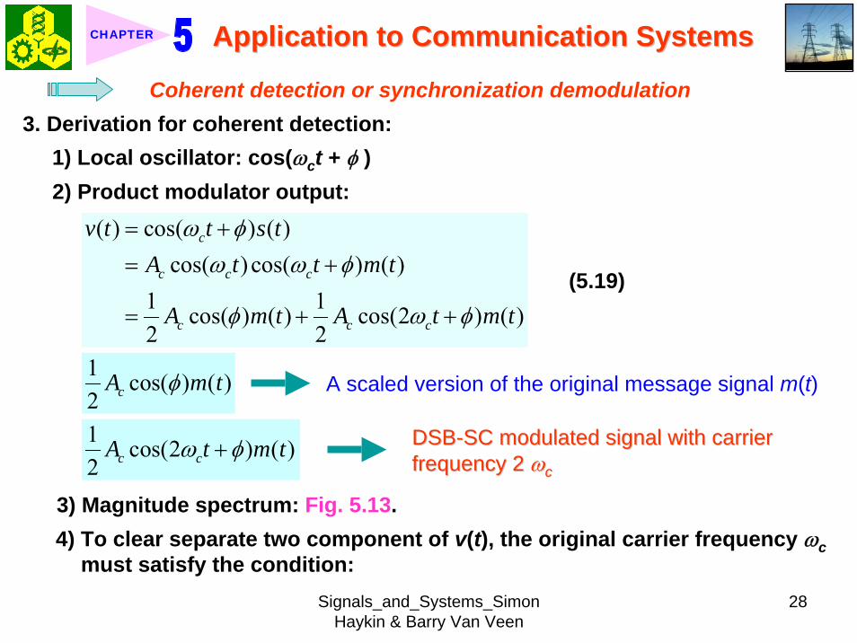
Signals_and_Systems_Simon Haykin amp Barry Van Veen
28
Application to Communication SystemsApplication to Communication SystemsCHAPTER
Coherent detection or synchronization demodulation3 Derivation for coherent detection
1) Local oscillator cos(ωct + φ )2) Product modulator output
( ) cos( ) ( )cos( ) cos( ) ( )
1 1cos( ) ( ) cos(2 ) ( )2 2
c
c c c
c c c
v t t s tA t t m t
A m t A t m t
ω φω ω φ
φ ω φ
= += +
= + +(519)
1 cos( ) ( )2 cA m tφ
1 cos(2 ) ( )2 c cA t m tω φ+
A scaled version of the original message signal m(t)
DSBDSB--SC modulated signal with carrier SC modulated signal with carrier frequency 2 frequency 2 ωωcc
3) Magnitude spectrum Fig 5134) To clear separate two component of v(t) the original carrier frequency ωc
must satisfy the condition
Signals_and_Systems_Simon Haykin amp Barry Van Veen
29
Application to Communication SystemsApplication to Communication SystemsCHAPTER
Figure 513 (p 442)Figure 513 (p 442)Magnitude spectrum of the product modulator output v(t) in the coherent detector of Fig 512(b)
v equiv ω p equiv π
2 c m mω ω ωminus gt c mω ωgt (520) ωωmm equivequiv message bandwidthmessage bandwidth
4 Specification of low-pass filter1) 1) The cutoff frequency must be The cutoff frequency must be ωωm m 2) The transition band must be 2) The transition band must be ωωm m ≦≦ ωω ≦≦ ωωc c ωωm m
Thus the overall output in Thus the overall output in Fig 512(b)Fig 512(b) is given byis given by1( ) cos( ) ( )2o cv t A m tφ= (521)
cosφ equiv attenuation factor
Signals_and_Systems_Simon Haykin amp Barry Van Veen
30
Application to Communication SystemsApplication to Communication SystemsCHAPTER
5 (1) Demodulated signal vo(t) is proportional to m(t) when the error phase φis a constant
(2) Demodulated signal is maximum when φ = 0 and has a minimum zero when φ = plusmn π2
Example 53 Sinusoidal DSB-SC ModulationConsider again the sinusoidal modulating signal
0 0( ) cos( )m t A tω=
( ) cos( )c cc t A tω=with amplitude A0 and frequency ω0 see Fig 514(a) The carrier wave is
with amplitude Ac and frequency ωc see Fig 514(b) Investigate the time-domain and frequency-domain characteristics of the corresponding DSB-SC modulated waveltltSolgtSolgt
clubs φ = plusmn π2 represents the quadrature null effect of the coherent detector
1 The modulated DSB-SC signal is defined by
0 0
0 0 0 0
( ) cos( ) cos( )1 1cos[( ) ] cos[( ) ]2 2
c c
c c c c
s t A A t t
A A t A A t
ω ω
ω ω ω ω
=
= + + minus
Signals_and_Systems_Simon Haykin amp Barry Van Veen
31
Application to Communication SystemsApplication to Communication SystemsCHAPTER
2 The Fourier transform of s(t) is given by
0 0 0
0 0
1( ) cos[ ( ) ( )]2
( ) ( )
c c c
c c
S j A Aω π δ ω ω ω δ ω ω ω
δ ω ω ω δ ω ω ω
= minus minus + + +
+ minus + + + minus
which consists of four weighted impulse functions at the frequencies ωc+ ω0-ωc- ω0 ωc- ω0 and- ωc+ ω0 as illustrated in the right-hand side of Fig Fig 514(c)514(c)
3 This Fourier transform differs from that depicted in the right-hand side of Fig Fig 56(c)56(c) for the corresponding example of full AM in one important respect The impulse functions at plusmn ωc due to the carrier are removed
4 Application of the sinusoidally modulated DSB-SC signal to the product modulator of Fig 512(b) yields the output (assuming φ = 0)
0 0 0
0 0 0 0 0
1( ) cos( ) cos[( ) ] cos[( ) ]21 cos[(2 ) ] cos( ) cos[(2 ) ] cos( )4
c c c c
c c c
v t A A t t t
A A t t t t
ω ω ω ω ω
ω ω ω ω ω ω
= + + minus
= + + + minus +
Signals_and_Systems_Simon Haykin amp Barry Van Veen
32
Application to Communication SystemsApplication to Communication SystemsCHAPTER
Figure 514 (p Figure 514 (p 443)443)Time-domain (on the left) and frequency-domain (on the right) characteristics of DSB-SC modulation produced by a sinusoidal modulating wave (a) Modulating wave (b) Carrier wave (c) DSB-SC modulated wave Note that ω= 2πƒ
v equiv ω p equiv π
Signals_and_Systems_Simon Haykin amp Barry Van Veen
33
Application to Communication SystemsApplication to Communication SystemsCHAPTER
5 The first two sinusoidal terms of v(t) are produced by the upper side frequency and the last two sinusoidal terms are produced by the lower side frequency
6 With ωcgt ω0 the first and third sinusoidal terms of frequencies 2ωc+ ω0 and 2ωc-ω0 respectively are removed by the low-pass filter of Fig 512(b)Fig 512(b) which leaves the second and fourth sinusoidal terms of frequency ω0 as the only output of the filter The coherent detector output thus reproduces the original modulating wave
7 Note however that this output appears as two equal terms one derived from the upper side frequency and the other from the lower side frequency We therefore conclude that for the transmission of the sinusoidal signal A0 cos(ω0t) only one side frequency is necessary (The issue will be discussed further in Section 57Section 57)
553 553 CostasCostas ReceiverReceiver1 Costas receiver Fig 515Fig 5152 This receiver consists of two coherent detector supplied with the same input
ie the incoming DSB-Sc wave
cos(2 ) ( )c cA f t m tπ but with individual local oscillator signals that are in phase duadrature with respect to each other
In-phase coherent detector (I-Channel) and quadrature-phase coherent detector (Q-Channel)
Signals_and_Systems_Simon Haykin amp Barry Van Veen
34
Application to Communication SystemsApplication to Communication SystemsCHAPTER
Figure 515 (p 445)Figure 515 (p 445)Costas receiver
v equiv ω p equiv π
Signals_and_Systems_Simon Haykin amp Barry Van Veen
35
Application to Communication SystemsApplication to Communication SystemsCHAPTER
56 56 QuadratureQuadrature--Carrier MultiplexingCarrier Multiplexing
Figure 516 (p 446)Figure 516 (p 446)Quadrature-carrier multiplexing system exploiting the quadrature null effect (a) Transmitter (b) Receiver assuming perfect synchronization with the transmitter
v equiv ω p equiv π
1 1 A A quadraturequadrature--carrier multiplexing or carrier multiplexing or quadraturequadrature--amplitude modulation (QAM) amplitude modulation (QAM) system enables two DSBsystem enables two DSB--SC modulated waves to occupy the same transmission SC modulated waves to occupy the same transmission bandwidth and yet it allows for their separation at the receivebandwidth and yet it allows for their separation at the receiver outputr output
BandwidthBandwidth--conservation schemeconservation scheme
Signals_and_Systems_Simon Haykin amp Barry Van Veen
36
Application to Communication SystemsApplication to Communication SystemsCHAPTER
2 Fig 5-16(a) Block diagram of the quadrature-carrier multiplexing systemFig 5-16(a) transmitter Fig 5-16(b) receiver
3 Multiplexed signal s(t)
(522) 1 2( ) ( ) cos( ) ( )sin( )c c c cs t A m t t A m t tω ω= +
where m1(t) and m2(t) denotes the two different message signals applied to the product modulations
clubsTransmission bandwidth = 2 ωm centered at ωc where ωm is the commonmessage bandwidth of m1(t) and m2(t)
4 The output of the top detector at receiver is 1
12 ( )cA m t
The output of the bottom detector at receiver is1
22 ( )cA m t
57 57 Other Variants of Amplitude Modulation Other Variants of Amplitude Modulation clubs Basic concept Full AM and DSB-SC rArr Wasteful of bandwidthclubs Given the amplitude and phase spectra of either lower or upper sideband
we can uniquely determine the other
Signals_and_Systems_Simon Haykin amp Barry Van Veen
37
Application to Communication SystemsApplication to Communication SystemsCHAPTER
clubs Single-sideband (SSB) modulation only one sideband is transmitted571 571 FrequencyFrequency--Domain Description of SSB ModulationDomain Description of SSB Modulation1 Consider a message signal m(t) with a spectrum M(jω) limited to the band
ωa le ω le ωb Fig 5-17 (a)2 DSB-SC modulated signal
( ) cos( )c cm t A tωtimes Fig 5-17 (b)
3 (1) Upper sideband the frequencies above ωc and below minus ωc(2) Upper sideband the frequencies below ωc and above minus ωc
Fig 5-17 (c)4 When only the lower sideband is transmitted the spectrum of the
corresponding SSB modulated wave is as shown in Fig 5-17 (d) 5 Advantages of SSB
(1) Reduced bandwidth requirement(2) Elimination of the high-power carrier waveDisadvantage od SSB(1) Cost and complexity of implementing both the transmitter and receiver
Signals_and_Systems_Simon Haykin amp Barry Van Veen
38
Application to Communication SystemsApplication to Communication SystemsCHAPTER
Figure 517 Figure 517 (p 447)(p 447)Frequency-domain characteristics of SSB modulation (a) Magnitude spectrum of message signal with energy gap from ndash ωa to ωa
(c) Magnitude spectrum of SSB modulated wave containing upper sideband only
(d) Magnitude spectrum of SSB modulated wave containing lower sideband only
(b) Magnitude spectrum of DSB-SC signal
v equiv ω p equiv π
Signals_and_Systems_Simon Haykin amp Barry Van Veen
39
Application to Communication SystemsApplication to Communication SystemsCHAPTER
6 Frequency-discrimination scheme for producing SSB modulation Fig 518clubs Bandpass filter is designed to pass the sideband selected for transmission
and suppress the remaining sidebandclubs Requirement in SSB signal the message signal applied to the product
modulator must have a energy gap in its spectrum Refer to Fig 517 (a)
Figure 518 (p 448)Figure 518 (p 448)System consisting of product modulator and bandpass filter for generating SSB modulated wave
v equiv ω p equiv π
572 572 TimeTime--Domain Description of SSB ModulationDomain Description of SSB Modulation1 Mathematical tool Hilbert transform
The Hilbert transform of a signal x(t) is defined by1 ( ) 1ˆ( ) ( )xx t d x t
t tτ τ
π τ πinfin
minusinfin= = lowast
minusint
Signals_and_Systems_Simon Haykin amp Barry Van Veen
40
Application to Communication SystemsApplication to Communication SystemsCHAPTER
The Fourier transform of 1(πt) is minus j times the signum function denoted
1 for 0sgn( ) 0 for 0
1 for 0
ωω ω
ω
+ gt⎧⎪= =⎨⎪minus lt⎩
2 Passing x(t) through a Hilbert transformer is equivalent to the combination of the following two operations in frequency domain1) Keeping X(jω)unchanged for all ω 2) Shifting areX(jω) (ie the phase spectrum of x(t)) by +90deg for negative
frequencies and minus 90deg for positive frequencies clubs Hilbert transformer = Wideband minus 90deg phase shifter 573 573 Vestigial Sideband ModulationVestigial Sideband Modulation1 When the message signal contains significant components at extremely
low frequencies the upper and lower sidebands meet at the carrier frequency
Using SSB is inappropriateUsing SSB is inappropriateEx TV signals or
wideband dataUsing VSB (Vestigial sideband) modulation is appropriateUsing VSB (Vestigial sideband) modulation is appropriate
Signals_and_Systems_Simon Haykin amp Barry Van Veen
41
Application to Communication SystemsApplication to Communication SystemsCHAPTER
2 VSB is a compromise between SSB and DSB-SC forms of modulationIn VSB modulation one sideband is passes almost completely whereas just a trace or vestige of the other sideband is retained
3 Fig 519 illustrates a VSB modulated wave s(t) in relation to the message signal m(t)
v equiv ω p equiv π
Figure 519 (p 449)Figure 519 (p 449)Spectral content of VSB modulated wave (a) Magnitude spectrum of message signal (c) Magnitude spectrum of VSB modulated wave containing a vestige of the lower sideband
clubs The lower sideband is modified into the vestigial sideband4 Transmission bandwidth of VSB modulated wave T m vω ω ω= + (523)
where ωm is the message bandwidth and ωu is the width of the vestigial sideband
Signals_and_Systems_Simon Haykin amp Barry Van Veen
42
Application to Communication SystemsApplication to Communication SystemsCHAPTER
5 Generation of VSB modulated wave Fig 520
Figure 520 (p 450)Figure 520 (p 450)System consisting of product modulator and sideband shaping filter for generating VSB modulated wave
v equiv ω p equiv π
Passing a DSBPassing a DSB--SC modulated wave through a sidebandSC modulated wave through a sideband--shaping filtershaping filter6 The sideband-shaping filter is designed so that the original message
spectrum M(jω) is reproduced on the demodulation as a result of the superposition of two spectra
1) The positive-frequency part of S(jω) (ie the Fourier transform of the transmitted signal s(t)) shifted downward in frequency by ωc
2) The negative-frequency part of S(jω) shifted upward in frequency by ωc
Fig 521 A reflection of the vestige of the lower sideband makes up for the missing parts of the upper sideband
Signals_and_Systems_Simon Haykin amp Barry Van Veen
43
Application to Communication SystemsApplication to Communication SystemsCHAPTER
Figure 521 (p 450)Figure 521 (p 450)Superposition of the two spectra shown in parts (a) and (b) of the figure results in the original message spectrum (shown dashed) upon demodulation
58 58 PulsePulse--Amplitude Modulation Amplitude Modulation clubs Basic concept
Basic role in the operation of AM Frequency-shiftingBasic role in the operation of PAM Sampling
581 581 Sampling RevisitedSampling Revisited1 Sampling theorem
In view point of PAMIn view point of PAM
Signals_and_Systems_Simon Haykin amp Barry Van Veen
44
Application to Communication SystemsApplication to Communication SystemsCHAPTER
1) A band-limited signal of finite energy that has no radian frequency components higher than ωm is uniquely determined by the values of the signal at instants of time separated by π ωm seconds
2) A band-limited signal of finite energy that has no radian frequency components higher than ωm may be completely recovered from a knowledge of its samples taken at the rate of ωm π per seconds
clubs Part 1) rArr Be exploited in the transmitter of a PAM clubs Part 2) rArr Be exploited in the Receiver of a PAM2 To combat the effects of aliasing in practice we use two corrective measures1) Prior to sampling a low-pass antialiasing filter is used to attenuate those high-
frequency components of the signal which lie outside the band of interest2) The filtered signal is sampled at a rate slightly higher than the Nyquist rate3 Generation of a PAM signal Fig 522Fig 522Example 54 Telephonic CommunicationThe highest frequency component of a speech signal needed for telephonic communication is about 31 kHz Suggest a suitable value for the sampling rate ltltSolgtSolgt
Signals_and_Systems_Simon Haykin amp Barry Van Veen
45
Application to Communication SystemsApplication to Communication SystemsCHAPTER
Figure 522 (p 451)Figure 522 (p 451)System consisting of antialiasing filter and sample-and-hold circuit for converting a message signal into a flattopped PAM signal
1 The highest frequency component of 31 kHz corresponds to 362 10 radsmω π= times
Correspondingly the Nyquist rate is
62 kHzmωπ
=
2 A suitable value for the sampling rate-one slightly higher than the Nyquistrate-may be 8 kHz a rate that is the international standard for telephone speech signals
Signals_and_Systems_Simon Haykin amp Barry Van Veen
46
Application to Communication SystemsApplication to Communication SystemsCHAPTER
582 582 Mathematical Description of PAMMathematical Description of PAM1 The carrier wave used in PAM consists of a sequence of short pulses of
fixed duration in terms of which PAM is formally defined as followsPAM is a form of pulse modulation in which the amplitude of the PAM is a form of pulse modulation in which the amplitude of the pulsed carrier is pulsed carrier is varied in accordance with instantaneous sample values of the mesvaried in accordance with instantaneous sample values of the message signalsage signal the duration of the pulsed carrier is maintained constant throughout
Fig 523Fig 523
Figure 523 (p452) Figure 523 (p452) Waveform of flattopped PAM signal with pulse duration T0 and sampling period Ts
Signals_and_Systems_Simon Haykin amp Barry Van Veen
47
Application to Communication SystemsApplication to Communication SystemsCHAPTER
2 Mathematical representation of the PAM
( ) [ ] ( )sn
s t m n b t nTinfin
=minusinfin
= minussum (524) s(t) equiv PAM signal m(t) equiv
message signal
Ts equiv sampling period m[n] equiv the values of m(t) at t = nTs h(t) equiv rectangular pulse of the unit amplitude and duration T0
3 Rectangular pulse
01 0( )
0 otherwiset T
h tlt lt⎧
= ⎨⎩
(525) Fig 524 (a)Fig 524 (a)
clubs Eq (524) is a sample-and-hold operationAnalogous to zeroAnalogous to zero--orderorder--holdhold--
based reconstruction in Sec 46based reconstruction in Sec 46
差異差異hh((tt) ) 的的TTss與與TT00
4 Impulse-sampled version of message signal m(t)
( ) [ ] ( )sn
m t m n t nTδ δinfin
=minusinfin
= minussum (526)
5 PAM signal( ) [ ] ( )
( ) ( )
sn
s t m n b t nT
m t b tδ
infin
=minusinfin
= minus
=
sum(527)
Convolution of impulse-sampled version mδ(t) and h(t)
Time domain Time domain operationoperation
Signals_and_Systems_Simon Haykin amp Barry Van Veen
48
Application to Communication SystemsApplication to Communication SystemsCHAPTER
Figure 524 (p 453)(a) Rectangular pulse h(t) of unit amplitude and duration T0 (b) Magnitude spectrum |H(jω)| and phase spectrum argH(jω) of pulse h(t)
v equiv ω p equiv π
Signals_and_Systems_Simon Haykin amp Barry Van Veen
49
Application to Communication SystemsApplication to Communication SystemsCHAPTER
6 FT of PAM signal( ) ( ) ( )S j M j H jδω ω ω= (528)
where( ) ( )FTS j s tω larr⎯rarr ( ) ( )FTM j m tδ δω larr⎯rarr ( ) ( )FTH j h tω larr⎯rarr
7 Impulse sampling of the message signal m(t) introduces periodicity into the spectrum as given by
1( ) ( ( ))sks
M j M j kTδ ω ω ω
infin
=minusinfin
= minussum (529) 1Ts equiv sampling rate ωs = 2πTs rads
1( ) ( ( )) ( )sks
S j M j k H jT
ω ω ω ωinfin
=minusinfin
= minussum (530)
( ) ( )FTM j m tω larr⎯rarrwhere
clubs Suppose that m(t) is strictly band limited and that the sampling rate 1Ts is greater than the Nyquist rate Then passing s(t) through a reconstruction filter chosen as an ideal low-pass filter with cutoff frequency ωm and gain Ts we find that the spectrum of the resulting filter output is equal to M(jω)H(jω)
Signals_and_Systems_Simon Haykin amp Barry Van Veen
50
Application to Communication SystemsApplication to Communication SystemsCHAPTER
8 From Eq (525) we find that0 2
0 0( ) sin ( (2 )) j TH j T c T e ωω ω π minus= (531) Fig 524(b) magnitude and phase of H(jω)
clubs Using PAM to represent a continuous-time message signal we introduce amplitude distortion as well as a delay of T02
clubs The frequency distortion caused by the use of flat-topped sampled in the generation of a PAM wave illustrated in Fig 523Fig 523 is referred to as the aperture effect
583 583 Demodulation of PAM SignalDemodulation of PAM Signal1 Reconstruction scheme Fig 525Fig 525
Figure 525 (p 454)Figure 525 (p 454)System consisting of low-pass interpolation filter and equalizer for reconstructing a message signal from its flattopped sampled version
clubs The system consists of low-pass interpolation filter and equalizer connected in cascade
Signals_and_Systems_Simon Haykin amp Barry Van Veen
51
Application to Communication SystemsApplication to Communication SystemsCHAPTER
2 The cutoff frequency of low-pass filter = the highest frequency ωm of message signal
3 The equalizer is used to correct the aperture effect due to flat-topped sampling in the sample-and-hold circuit
4 The equalizer has the effect of decreasing the in-band loss of the interpolation filter as frequency increases in such a manner as to compensate for the aperture effect
5 Amplitude response of equalizer
0
0 0 0 0
1 1 1| ( ) | | sinc( 2) | 2 | sin( 2) |
TH j T T T T
ωω ω ω
= =
Frequency response Eq (531)
Example 55 Equalization for PAM TransmissionThe duty cycle in a PAM signal namely T0 Ts is 10 Evaluate the peak amplification required for equalizationltltSolgtSolgt1 At ωm = π Ts which corresponds to the highest frequency component of the
message signal for a sampling rate equal to the Nyquist rate we find from Eq (531) that the magnitude response of the equalizer at ωm normalized to that at zero frequency is
Signals_and_Systems_Simon Haykin amp Barry Van Veen
52
Application to Communication SystemsApplication to Communication SystemsCHAPTER
Figure 526 (p 455)Figure 526 (p 455)Normalized equalization (to compensate for aperture effect) plotted against the duty cycle T0Ts
Signals_and_Systems_Simon Haykin amp Barry Van Veen
53
Application to Communication SystemsApplication to Communication SystemsCHAPTER
0
0 0
( 2)( )1sin (05 ) sin[( 2)( )]
s
s s
T Tc T T T T
ππ
=
where the ratio T0 Ts is equal to the duty cycle of the sampling pulses 2 In Fig 526Fig 526 this result is plotted as a function of the duty cycle T0 Ts Ideally it
should be equal to unity for all values of T0 Ts 3 For a duty cycle of 10 it is equal to 10041 It follows that for duty cycles of less
than 10 the magnitude equalization required is less than 10041 in which case the aperture effect is usually considered to be negligible
59 59 Multiplexing Multiplexing clubs Three basic types of multiplexing1 Frequency-division multiplexing in which the signals are separated by
allocating them to different frequency bands This is illustrated in Fig 527(a) for the case of six different message signals Frequency-division multiplexing favors the use of CW modulation where each message signal is able to use the channel on a continuous-time basis
2 Time-division multiplexing wherein the signals are separated by allocating them to different time slots within a sampling interval
Signals_and_Systems_Simon Haykin amp Barry Van Veen
54
Application to Communication SystemsApplication to Communication SystemsCHAPTER
This second type of multiplexing is illustrated in Fig 527(b) for the case of six different message signals Code-division multiplexing which relies on the assignment of different codes to the individual users of the channel
3 Code-division multiplexing which relies on the assignment of different codes to the individual users of the channel
591 591 FrequencyFrequency--Domain Multiplexing (FDM)Domain Multiplexing (FDM)1 Block diagram Fig 528Fig 5282 Incoming message signals low-pass variety3 Low-pass filter to remove high-frequency components such that the signal
in each channel does not disturb each other4 MOD (modulator) shift the frequency ranges of the signals so as to occupy
mutually exclusive frequency intervalsSSB is often used in this stageEx Voice input is usually assigned a bandwidth of 4 kHz
5 Band-pass filters are used to restrict the band of each modulated wave to its prescribed range
6 Band-pass filters in receiver separate the message signals7 DEM (demodulator) to recover signalsclubs FDM in Fig 528 operates in only one direction
Signals_and_Systems_Simon Haykin amp Barry Van Veen
55
Application to Communication SystemsApplication to Communication SystemsCHAPTER
Figure 527 (p 456)Figure 527 (p 456)Two basic forms of multiplexing (a) Frequency-division multiplexing (with guardbands) (b) Time-division multiplexing no provision is made here for synchronizing pulses
Signals_and_Systems_Simon Haykin amp Barry Van Veen
56
Application to Communication SystemsApplication to Communication SystemsCHAPTER
Figure 528 (p 457)Figure 528 (p 457)Block diagram of FDM system showing the important constituents of the transmitter and receiver
Signals_and_Systems_Simon Haykin amp Barry Van Veen
57
Application to Communication SystemsApplication to Communication SystemsCHAPTER
Example 56 SSB-FDM System
ltltSolgtSolgt
An FDM system is used to multiplex 24 independent voice signals SSB modulation is used for the transmission Given that each voice signal is allotted a bandwidth 4kHz calculate the overall transmission bandwidth of the channel
With each voice signal allotted a bandwidth of 4 kHz the use of SSB modulation requires a bandwidth of 4 kHz for its transmission Accordingly the overall transmission bandwidth provided by the channel is 24 X 4 = 96 kHz 592 592 TimeTime--Domain Multiplexing (TDM)Domain Multiplexing (TDM)clubs Basic to the operation of a TDM system is the sampling theoremclubs The transmission of the message samples engages the transmission channel for
only a fraction of the sampling interval on a periodic basis equal to the width T0 of a PAM modulating pulse
1 Block diagram Fig 529Fig 5292 Commutator is usually implemented by means of electronic switching
circuitry3 The function of commutator is two folds
Signals_and_Systems_Simon Haykin amp Barry Van Veen
58
Application to Communication SystemsApplication to Communication SystemsCHAPTER
Figure 529 (p 458)Figure 529 (p 458)Block diagram of TDM system showing the important constituents of the transmitter and receiver
(1) To take a narrow sample of each of the M input message signals at a rate 1Tsthat is slightly higher than ωcπ where ωc is the cutoff frequency of the input low-pass filter
(2) To sequentially interleave these M samples inside a sampling interval Ts4 Pulse modulator transform the multiplexed signal into a form suitable for
transmission over the common channel
Signals_and_Systems_Simon Haykin amp Barry Van Veen
59
Application to Communication SystemsApplication to Communication SystemsCHAPTER
clubs The use of time-division multiplexing introduces a bandwidth expansion factor M because the scheme must squeeze M samples derived from M independent message sources into a time slot equal to one sampling interval
5 Pulse demodulator performs the inverse operation of the pulse modulator6 Decommutator distributes the narrow samples produced by pulse demodulator to the appropriate low-pass reconstruction filter7 Synchronization between the timing operations of the transmitter and
receiver in a TDM system is essential for satisfactory performance of the system
Inserting an extra pulse into each sampling interval on a regular basisBandwidth expansion factor is increased to M + 1
clubs The TDM system is hghly sensitive to the dispersion in the common transmission channel
Example 57 Comparison of TDM with FDMATDM system is used to multiplex four independent voice signals using PAM Each voice signal is sampled at the rate of 8 kHz The system incorporates a synchronizing pulse train for its proper operation
Signals_and_Systems_Simon Haykin amp Barry Van Veen
60
Application to Communication SystemsApplication to Communication SystemsCHAPTER
(a) Determine the timing relationships between the synchronizing pulse train and the impulse trains used to sample the four voice signals
(b) Calculate the transmission bandwidth of the channel for the TDM system and compare the result with a corresponding FDM system using SSBmodulation
ltltSolgtSolgt(a) The sampling period is
31 125 s
8 10sT s μ= =times
In this example the number of voice signals is M = 4 Hence dividing the sampling period of 125 μs among these voice signals and the synchronizing pulse train we obtain the time slot allocated to each one of them
0 1125 25 s
5
sTTM
μ
=+
= =
Signals_and_Systems_Simon Haykin amp Barry Van Veen
61
Application to Communication SystemsApplication to Communication SystemsCHAPTER
Figure 530Figure 530 shows the timing relationships between the synchronizing pulse train and the four impulse trains used to sample the different voice signals in a single frame Each frame includes time slots of common duration T0 = 25 μs which are allocated to the pulse-modulated signals and synchronizing pulse
Figure 530 (p 459)Figure 530 (p 459)Composition of one frame of a multiplexed PAM signal incorporating four voice-signals and a synchronizing pulse
Signals_and_Systems_Simon Haykin amp Barry Van Veen
62
Application to Communication SystemsApplication to Communication SystemsCHAPTER
(b) As a consequence of the time-bandwidth product (see Section 317) there is an inverse relationship between the duration of a pulse and the bandwidth (ie cutoff frequency) of the channel needed for itstransmission Accordingly the overall transmission bandwidth of the channel is
0
21 1 MHz 40 kHz
25
TTf
T
ωπ
=
= = =
In contrast the use of an FDM system based on SSB modulation requires a channel bandwidth equal to M times that of a single voice signal-that is 4 X 4 = 16 kHz Thus the use of PAM-TDM requires a channel bandwidth that is 40 16 = 25 times that of SSB-FDMIn practice pulse-code modulation is commonly used as the method of modulation for TDM this results in a further increase in channel bandwidth depending on the length of the code word used in the digital representation of each pulse in the PAM signal
Signals_and_Systems_Simon Haykin amp Barry Van Veen
63
Application to Communication SystemsApplication to Communication SystemsCHAPTER
510 510 Pulse and Group Delays Pulse and Group Delays 1 Whenever a signal is transmitted through a dispersive (ie frequency
selective) system some delay is introduced into the output signal in relation to the input signal
2 The delay is determined by the phase response of the system3 Phase response of a dispersive communication channel
( ) arg ( )H jφ ω ω= (532)
A signal is transmitted through the channel at a frequency ωc The signal received at the channel lags the transmitted signal by φ(ωc) The time delay is called phase delay formally defined as
( )cp
c
φ ωτω
= minus (533)
The phase delay is not necessarily the true signal delayclubs Case study for DSB-SC1 Transmitted signal
0( ) cos( ) cos( )cs t A t tω ω= (534)
ωc equiv carrier frequency ω0 equiv sinusoidal modulation frequency
A = AcA0
Signals_and_Systems_Simon Haykin amp Barry Van Veen
64
Application to Communication SystemsApplication to Communication SystemsCHAPTER
1 21 1( ) cos( ) cos( )2 2
s t A t A tω ω= +
1 0cω ω ω= + (535) where
2 0cω ω ω= minus (536)
Upper frequency
Lower frequency
2 Let the s(t) be transmitted through the channel with phase response φ (ω) Accordingly the signal received at the channel output is
1 1 2 21 1( ) cos( ( )) cos( ( ))2 2
y t A t A tω φ ω ω φ ω= + + +
1 2 1 20
( ) ( ) ( )1 ( )( ) cos cos2 2cy t A t tφ ω φ ω φ ω φ ωω ω+⎛ ⎞ ⎛ ⎞= + +⎜ ⎟ ⎜ ⎟
⎝ ⎠ ⎝ ⎠(537)
3 Two observations from Eq (537)1) The carrier component at frequency ωc in y(t) lags its counterpart in s(t) by
frac12 (φ (ω1) + φ (ω2)) which represents a time delay equal to
1 2 1 2
c 1 2
( )+ ( ) ( )+ ( )2 +
φ ω φ ω φ ω φ ωω ω ω
minus = minus (538)
Signals_and_Systems_Simon Haykin amp Barry Van Veen
65
Application to Communication SystemsApplication to Communication SystemsCHAPTER
2) The message component at frequency ω0 in y(t) lags its counterpart in s(t) by frac12 (φ (ω1) minus φ (ω2)) which represents a time delay equal to
1 2 1 2
0 1 2
( ) ( ) ( ) ( )2
φ ω φ ω φ ω φ ωω ω ωminus minus
minus = minusminus
(539)
4 Suppose that ω0 lt ωc rArr the side frequencies are close together with ω c between them Such a modulated signal is said to be a narrowband signal The phase response φ (ω) in the vicinity of ω = ωc is approximated by two-term Taylor series expansion
( )( ) ( ) ( )c
c cd
d ω ω
φ ωφ ω φ ω ω ωω =
= + times minus (540)
Phase delay = ( ) c cφ ω ωminus
5 The time delay introduced by the message signal (ie he ldquoenveloperdquo of the modulated signal) is given by
( )
c
gd
d ω ω
φ ωτω =
= minus (541) The time delay τg is called the
envelope delay or group delay
Signals_and_Systems_Simon Haykin amp Barry Van Veen
66
Application to Communication SystemsApplication to Communication SystemsCHAPTER
6 When a modulated signal is transmitted through a communication channel there are two different delays to be considered1) The carrier or phase delay τp defined by Eq (533)2) The envelope or group delay τg defined by Eq (541)
clubs The group delay is the true signal delay
Example 58 Phase and Group Delays for Ban-pass Channel
ltltSolgtSolgt
The phase response of a band-pass communication channel is defined by 2 2
1( ) tan c
c
ω ωφ ωωω
minus ⎛ ⎞minus= minus ⎜ ⎟
⎝ ⎠The signal s(t) defined in Eq (534) is transmitted through this channel with
475 radscω = 0 025 radsω =andCalculate (a) the phase delay and (b) the group delay
(a) At ω = ωc φ (ωc) = 0 According to Eq (533) the phase delay τ p is zero (b) Differentiating φ (ω) with respect to ω we get
Signals_and_Systems_Simon Haykin amp Barry Van Veen
67
Application to Communication SystemsApplication to Communication SystemsCHAPTER
2 2
2 2 2 2 2
( )( )( )
c c
c c
dd
ω ω ωφ ωω ω ω ω ω
+= minus
+ minus
Using thing result in Eq (541) we find that the group delay is 2 2 04211
475gc
sτω
= = =
1 One waveform shown as a solid curve was obtained by multiplying the transmitted signal s(t) by the carrier wave cos(ωct)
2 The second waveform shown as a dotted curve was obtained by multiplying the received signal y(t) by the carrier wave cos(ωct)
To display the results obtained in parts (a) and (b) in graphical form Fig 531Fig 531shows a superposition of two waveforms obtained as follows
The figure clearly shows that the carrier (phase) delay τ p is zero and the envelope of the received signal y(t) is lagging behind that of the transmitted signal by τs seconds For the presentation of waveforms in this figure we purposely did not use a filter to suppress the high frequency components resulting from the multiplications described under points 1 and 2 because of the desire to retain a contribution due to the carrier for display
Signals_and_Systems_Simon Haykin amp Barry Van Veen
68
Application to Communication SystemsApplication to Communication SystemsCHAPTER
Figure 531 Figure 531 (p 463)(p 463)Highlighting the zero carrier delay (solid curve) and group delay τg (dotted curve) which are determined in accordance with Example 58
Signals_and_Systems_Simon Haykin amp Barry Van Veen
69
Application to Communication SystemsApplication to Communication SystemsCHAPTER
clubs Not also that the separation between the upper side frequency ω1 = ωc + ω0 = 500 rads and the lower side frequency ω2 = ωc minus ω0 = 450 rads is about 10 of the carrier frequency ωc = 475 rads which justifies referring to the modulated signal in this example as a narrowband signal
5101 5101 Some Practical ConsiderationsSome Practical Considerationsclubs What is the practical importance of group delay 1 Eq (541) for determining group delay applies strictly to narrowband
modulated signal2 The message bandwidth may be comparable to the carrier frequency In
this situation the group delay is formulated as a frequency-dependent parameter ie ( )d( )g d
φ ωτ ωω
= minus (542)
3 When a wideband modulated signals transmitted through a dispersive channel the frequency components of the message signal are delayed by different amounts at the channel output
Delay distortionFig 532Fig 532 Group delay response of voice-grade telephone channel
Signals_and_Systems_Simon Haykin amp Barry Van Veen
70
Application to Communication SystemsApplication to Communication SystemsCHAPTER
Figure 532 (p 464)Group delay response of voice-grade telephone channel (Adapted from J C Bellamy Digital Telephony Wiley 1982)
511 511 Exploring Concepts with MATLABExploring Concepts with MATLAB5111 5111 Full AMFull AMclubs Sinusoidal modulation
clubs To reconstruct a faithful version of the original message signal in the receiver we have to use a delay equalizer
0( ) [1 cos( )]cos( )c cs t A t tμ ω ω= +1 AM experiment
1cA =
08 radscω π= 0 01 radsω π=Carrier amplitude
Carrier frequency Modulation amplitude
Signals_and_Systems_Simon Haykin amp Barry Van Veen
71
Application to Communication SystemsApplication to Communication SystemsCHAPTER
2 We wish to display and analyze 10 full cycles of the AM wave corresponding to a total duration of 200 s Choosing a sampling rate 1Ts = 10 Hz we have a total of N = 2000 time samples The frequency band of interest is minus 10 π ≦ ω ≦ 10 π Since the separation between the carrier and either side frequency is equal to the modulation frequency ω0 = 01 π rads we would like to have a frequency resolution ωr = 001π rads To achieve this resolution we require the following number of frequency samples (see Eq (442))
20 2000001
s
r
M ω πω π
ge = =
3 We therefore choose M = 2000 To approximate the Fourier transform of the AM wave s(t) we may use a 2000-point DTFS The only variable in the AM experiment is the modulation factor μ with respect to which we wish to investigate three different situationsμ = 05 corresponding to under-modulationμ = 10 for which the AM system is on the verge of over-modulationμ = 20 corresponding to over-modulation
Signals_and_Systems_Simon Haykin amp Barry Van Veen
72
Application to Communication SystemsApplication to Communication SystemsCHAPTER
4 MATLAB commandsAc = 1 carrier amplitudewc = 08pi carrier frequencyw0 = 01pi modulation frequencymu = 05 modulation factort = 0011999s = Ac(1 + mucos(w0t))cos(wct)plot(ts)Smag = abs(fftshift(fft(s2000)))2000 Smag denotes the magnitude specturm of the AM wavew = 10[-1000999]2pi2000plot(wSmag)axis ([-30 30 0 08])
5 5 μμ = 05 = 05 case case Fig 533Fig 533μμ = 10 case = 10 case Fig 534Fig 534μμ = 20 case = 20 case Fig 535Fig 535
Discussion see pp 466-469 textbook
Signals_and_Systems_Simon Haykin amp Barry Van Veen
73
Application to Communication SystemsApplication to Communication SystemsCHAPTER
-30 -20 -10 0 10 20 300
02
04
06
0 50 100 150 200-2
-1
0
1
2
2 22 24 26 28 3
02
04
06
(a) Time (s)
Time domain
Frequency domain
(b) Frequency (rads)
Frequency domain
Frequency (rads)
Figure 533 (p 466)Amplitude modulation with 50 modulation (a) AM wave (b) magnitude spectrum of the AM wave and (c) expanded spectrum around the carrier frequency
μμ = 05 = 05 casecase
Signals_and_Systems_Simon Haykin amp Barry Van Veen
74
Application to Communication SystemsApplication to Communication SystemsCHAPTER
Figure 534 (p 467)Figure 534 (p 467)Amplitude modulation with 100 modulation (a) AM wave (b) magnitude spectrum of the AM wave and (c) expanded spectrum around the carrier frequency
Signals_and_Systems_Simon Haykin amp Barry Van Veen
75
Application to Communication SystemsApplication to Communication SystemsCHAPTER
Figure 535 (p 468)Amplitude modulation with 200 modulation (a) AM wave (b) magnitude spectrum of the AM wave and (c) expanded spectrum around the carrier frequency
Signals_and_Systems_Simon Haykin amp Barry Van Veen
76
Application to Communication SystemsApplication to Communication SystemsCHAPTER
5112 5112 DSBDSB--SC ModulationSC Modulation1 Sinusoidal modulation
0 0( ) cos( ) cos( )c cs t A A t tω ω=
2 MATLAB commands
Ac = 1 carrier amplitudewc = 08pi carrier frequency in radsA0 = 1 amplitude of modulating signalw0 = 01pi frequency of modulating signalt = 011999s = AcA0cos(wct)cos(w0t)plot(ts)Smag = abs(fftshift(fft(s2000)))2000w = 10[-1000999]2pi2000plot(wSmag)
3 3 DSBDSB--SC modulated waveSC modulated wave Fig 536Fig 536 Discussion see pp 466-469 textbook
4 Output of the product modulator in Fig 512 (b) with φ = 0
Signals_and_Systems_Simon Haykin amp Barry Van Veen
77
Application to Communication SystemsApplication to Communication SystemsCHAPTER
Figure 536 (p 469)DSB-SC modulation (a) DSB-SC modulated wave (b) magnitude spectrum of the modulated wave and (c) expanded spectrum around the carrier frequency
Signals_and_Systems_Simon Haykin amp Barry Van Veen
78
Application to Communication SystemsApplication to Communication SystemsCHAPTER
( ) ( ) cos( )cv t s t tω=
5 MATLAB commandsgtgt v = scos(wct)
6 Fig 537 (a) waveforms of v(t) Fig 537 (b) magnitude spectrum which readily shows that v(t) consists of the following components1) A sinusoidal component with frequency 01π rads representing the
modulating wave2) A new DSB-SC modulated wave with double carrier frequency of 16π rads
in actuality the side frequencies of this modulated wave are located at 15πand 17π rads
1) The frequency of the modulating wave lies inside the passband of the filter2) The upper and lower side frequencies of the new DSB-SC modulated wave
lie inside the stopband of the filter
Accordingly we may recover the sinusoidal modulating signal by passing v(t) through low-pass filter with the following requirements
Signals_and_Systems_Simon Haykin amp Barry Van Veen
79
Application to Communication SystemsApplication to Communication SystemsCHAPTER
Figure 537 (p 470)Coherent detection of DSB-SC modulated wave (a) and (b) Waveform and magnitude spectrum of signal produced at the output of produce modulator (c) and (d) waveform and magnitude spectrum of low-pass filter output
Signals_and_Systems_Simon Haykin amp Barry Van Veen
80
Application to Communication SystemsApplication to Communication SystemsCHAPTER
The issue of how to design a filter with these requirements will be considered in detail in Chapter 8 For the present it suffices to say that the preceding requirements can be met by using the following MATLAB commands
gtgt [ba] = butter(30025)gtgt output = filter(bav)
The first command produces s special type of filter called a Butterworth filter For the experiment considered here the filter order is 3 and its normalized cutoff frequency of 0025 is calculated as follows
Actual cutoff frequency of filter 025 radsHalf the sampling rate 10 rads
0025
ππ
=
=
The second command computes the filterrsquos output in response to the product modulator output v(t) (We will revisit the design of this filter in Chapter 8) Figure 537(c) displays the waveform of the low-pass filter output this waveform represents a sinusoidal signal of frequency 005 Hz an observation that is confirmed by using the ffr command to approximate the spectrum of the filter output The result of the computation is shown in Fig 537(d)Fig 537(d)
Signals_and_Systems_Simon Haykin amp Barry Van Veen
81
Application to Communication SystemsApplication to Communication SystemsCHAPTER
7 In Fig 538 we explore another aspect of DSB-SC modulation namely the effect of varying the modulation frequency Figure 538(a) shows five cycles of a DSB-SC modulated wave that has the same carrier frequency as that in Fig 536(a) but the modulation frequency has been reduced to 0025 Hz( ie a radian frequency of 005π) Figure 538(b) shows the magnitude spectrum of this second DSB-SC modulated wave and its zoomed-in version is shown in Fig 538(c) Comparing this latter figure with Fig 536(c) we see clearly that decreasing the modulation frequency has the effect of moving the upper and lower side frequencies closer together which is consistent with modulation theory
5113 5113 Phase and Group DelayPhase and Group Delay1 In Example 58 we studied the phase and group delays for a band-pass
channel with phase response 2 2
1( ) tan c
c
ω ωφ ωωω
minus ⎛ ⎞minus= minus ⎜ ⎟
⎝ ⎠2 At ω = ωc the phase delay is τ p = 0 and the group delay is τ s = 04211s One
of the wave forms displayed in Fig 531Fig 531 is
1( ) ( ) cos( )cx t s t tω=
Signals_and_Systems_Simon Haykin amp Barry Van Veen
82
Application to Communication SystemsApplication to Communication SystemsCHAPTER
Figure 538 (p 472)Effect of varying the modulation frequency compared with that in Fig 537 (a) and (b) Waveform and magnitude spectrum of DSB-SC modulated wave with a modulation frequency one-half that used in Fig 536 (c) expanded spectrum around the carrier frequency
Signals_and_Systems_Simon Haykin amp Barry Van Veen
83
Application to Communication SystemsApplication to Communication SystemsCHAPTER
where (see page 461)
1 2( ) [cos( ) cos( )]2As t t tω ω= +
and ω1 = ωc + ω0 and ω2 = ωc - ω0 The waveform shown in the figure as a solid curve is a plot of x1(t) The other waveform also displayed in Fig 531Fig 531 is
2
1 1 2 2
( ) ( ) cos( )
[cos( ( )) cos( ( ))]cos( )2
c
c
x t y t tA t t t
ω
ω φ ω ω φ ω ω
=
= + + +
where the angle φ (ω1) and φ (ω2) are the values of the phase response φ (ω) at ω = ω1 and ω = ω2 respectively The waveform shown as a dotted curve in the figure is a plot of x2(t)
3 The generation of x1(t) and x2(t) in MATLAB is achieved with the following commands with A2 set equal to unity
Signals_and_Systems_Simon Haykin amp Barry Van Veen
84
Application to Communication SystemsApplication to Communication SystemsCHAPTER
wc = 475w0 = 025w1 = wc + w0w2 = wc - w0t = -10 0001 10o1 = -atan((w1^2 - wc^2)(w1wc))o2 = -atan((w2^2 - wc^2)(w2wc))s = cos(w1t) + cos(w2t)y = cos(w1t + o1) + cos(w2t + o2)x1 = scos(478t)x2 = ycos(475t)plot(tx1b)hold on plot(tx2k)hold offxlabel(Time)ylabel(Amplitude)
Note that we have set (A2) = 1 for convenience of presentation The function atan in the first two commands returns the arctangent Note also that the computation of both x1 and x2 involve element-by-element multiplications ndash hence the use of period followed by an asterisk
Signals_and_Systems_Simon Haykin amp Barry Van Veen
85
Application to Communication SystemsApplication to Communication SystemsCHAPTER
Signals_and_Systems_Simon Haykin amp Barry Van Veen
86
Application to Communication SystemsApplication to Communication SystemsCHAPTER
Signals_and_Systems_Simon Haykin amp Barry Van Veen
87
Application to Communication SystemsApplication to Communication SystemsCHAPTER
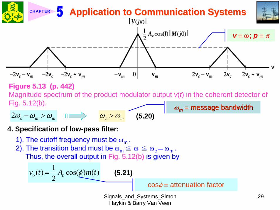
Signals_and_Systems_Simon Haykin amp Barry Van Veen
29
Application to Communication SystemsApplication to Communication SystemsCHAPTER
Figure 513 (p 442)Figure 513 (p 442)Magnitude spectrum of the product modulator output v(t) in the coherent detector of Fig 512(b)
v equiv ω p equiv π
2 c m mω ω ωminus gt c mω ωgt (520) ωωmm equivequiv message bandwidthmessage bandwidth
4 Specification of low-pass filter1) 1) The cutoff frequency must be The cutoff frequency must be ωωm m 2) The transition band must be 2) The transition band must be ωωm m ≦≦ ωω ≦≦ ωωc c ωωm m
Thus the overall output in Thus the overall output in Fig 512(b)Fig 512(b) is given byis given by1( ) cos( ) ( )2o cv t A m tφ= (521)
cosφ equiv attenuation factor
Signals_and_Systems_Simon Haykin amp Barry Van Veen
30
Application to Communication SystemsApplication to Communication SystemsCHAPTER
5 (1) Demodulated signal vo(t) is proportional to m(t) when the error phase φis a constant
(2) Demodulated signal is maximum when φ = 0 and has a minimum zero when φ = plusmn π2
Example 53 Sinusoidal DSB-SC ModulationConsider again the sinusoidal modulating signal
0 0( ) cos( )m t A tω=
( ) cos( )c cc t A tω=with amplitude A0 and frequency ω0 see Fig 514(a) The carrier wave is
with amplitude Ac and frequency ωc see Fig 514(b) Investigate the time-domain and frequency-domain characteristics of the corresponding DSB-SC modulated waveltltSolgtSolgt
clubs φ = plusmn π2 represents the quadrature null effect of the coherent detector
1 The modulated DSB-SC signal is defined by
0 0
0 0 0 0
( ) cos( ) cos( )1 1cos[( ) ] cos[( ) ]2 2
c c
c c c c
s t A A t t
A A t A A t
ω ω
ω ω ω ω
=
= + + minus
Signals_and_Systems_Simon Haykin amp Barry Van Veen
31
Application to Communication SystemsApplication to Communication SystemsCHAPTER
2 The Fourier transform of s(t) is given by
0 0 0
0 0
1( ) cos[ ( ) ( )]2
( ) ( )
c c c
c c
S j A Aω π δ ω ω ω δ ω ω ω
δ ω ω ω δ ω ω ω
= minus minus + + +
+ minus + + + minus
which consists of four weighted impulse functions at the frequencies ωc+ ω0-ωc- ω0 ωc- ω0 and- ωc+ ω0 as illustrated in the right-hand side of Fig Fig 514(c)514(c)
3 This Fourier transform differs from that depicted in the right-hand side of Fig Fig 56(c)56(c) for the corresponding example of full AM in one important respect The impulse functions at plusmn ωc due to the carrier are removed
4 Application of the sinusoidally modulated DSB-SC signal to the product modulator of Fig 512(b) yields the output (assuming φ = 0)
0 0 0
0 0 0 0 0
1( ) cos( ) cos[( ) ] cos[( ) ]21 cos[(2 ) ] cos( ) cos[(2 ) ] cos( )4
c c c c
c c c
v t A A t t t
A A t t t t
ω ω ω ω ω
ω ω ω ω ω ω
= + + minus
= + + + minus +
Signals_and_Systems_Simon Haykin amp Barry Van Veen
32
Application to Communication SystemsApplication to Communication SystemsCHAPTER
Figure 514 (p Figure 514 (p 443)443)Time-domain (on the left) and frequency-domain (on the right) characteristics of DSB-SC modulation produced by a sinusoidal modulating wave (a) Modulating wave (b) Carrier wave (c) DSB-SC modulated wave Note that ω= 2πƒ
v equiv ω p equiv π
Signals_and_Systems_Simon Haykin amp Barry Van Veen
33
Application to Communication SystemsApplication to Communication SystemsCHAPTER
5 The first two sinusoidal terms of v(t) are produced by the upper side frequency and the last two sinusoidal terms are produced by the lower side frequency
6 With ωcgt ω0 the first and third sinusoidal terms of frequencies 2ωc+ ω0 and 2ωc-ω0 respectively are removed by the low-pass filter of Fig 512(b)Fig 512(b) which leaves the second and fourth sinusoidal terms of frequency ω0 as the only output of the filter The coherent detector output thus reproduces the original modulating wave
7 Note however that this output appears as two equal terms one derived from the upper side frequency and the other from the lower side frequency We therefore conclude that for the transmission of the sinusoidal signal A0 cos(ω0t) only one side frequency is necessary (The issue will be discussed further in Section 57Section 57)
553 553 CostasCostas ReceiverReceiver1 Costas receiver Fig 515Fig 5152 This receiver consists of two coherent detector supplied with the same input
ie the incoming DSB-Sc wave
cos(2 ) ( )c cA f t m tπ but with individual local oscillator signals that are in phase duadrature with respect to each other
In-phase coherent detector (I-Channel) and quadrature-phase coherent detector (Q-Channel)
Signals_and_Systems_Simon Haykin amp Barry Van Veen
34
Application to Communication SystemsApplication to Communication SystemsCHAPTER
Figure 515 (p 445)Figure 515 (p 445)Costas receiver
v equiv ω p equiv π
Signals_and_Systems_Simon Haykin amp Barry Van Veen
35
Application to Communication SystemsApplication to Communication SystemsCHAPTER
56 56 QuadratureQuadrature--Carrier MultiplexingCarrier Multiplexing
Figure 516 (p 446)Figure 516 (p 446)Quadrature-carrier multiplexing system exploiting the quadrature null effect (a) Transmitter (b) Receiver assuming perfect synchronization with the transmitter
v equiv ω p equiv π
1 1 A A quadraturequadrature--carrier multiplexing or carrier multiplexing or quadraturequadrature--amplitude modulation (QAM) amplitude modulation (QAM) system enables two DSBsystem enables two DSB--SC modulated waves to occupy the same transmission SC modulated waves to occupy the same transmission bandwidth and yet it allows for their separation at the receivebandwidth and yet it allows for their separation at the receiver outputr output
BandwidthBandwidth--conservation schemeconservation scheme
Signals_and_Systems_Simon Haykin amp Barry Van Veen
36
Application to Communication SystemsApplication to Communication SystemsCHAPTER
2 Fig 5-16(a) Block diagram of the quadrature-carrier multiplexing systemFig 5-16(a) transmitter Fig 5-16(b) receiver
3 Multiplexed signal s(t)
(522) 1 2( ) ( ) cos( ) ( )sin( )c c c cs t A m t t A m t tω ω= +
where m1(t) and m2(t) denotes the two different message signals applied to the product modulations
clubsTransmission bandwidth = 2 ωm centered at ωc where ωm is the commonmessage bandwidth of m1(t) and m2(t)
4 The output of the top detector at receiver is 1
12 ( )cA m t
The output of the bottom detector at receiver is1
22 ( )cA m t
57 57 Other Variants of Amplitude Modulation Other Variants of Amplitude Modulation clubs Basic concept Full AM and DSB-SC rArr Wasteful of bandwidthclubs Given the amplitude and phase spectra of either lower or upper sideband
we can uniquely determine the other
Signals_and_Systems_Simon Haykin amp Barry Van Veen
37
Application to Communication SystemsApplication to Communication SystemsCHAPTER
clubs Single-sideband (SSB) modulation only one sideband is transmitted571 571 FrequencyFrequency--Domain Description of SSB ModulationDomain Description of SSB Modulation1 Consider a message signal m(t) with a spectrum M(jω) limited to the band
ωa le ω le ωb Fig 5-17 (a)2 DSB-SC modulated signal
( ) cos( )c cm t A tωtimes Fig 5-17 (b)
3 (1) Upper sideband the frequencies above ωc and below minus ωc(2) Upper sideband the frequencies below ωc and above minus ωc
Fig 5-17 (c)4 When only the lower sideband is transmitted the spectrum of the
corresponding SSB modulated wave is as shown in Fig 5-17 (d) 5 Advantages of SSB
(1) Reduced bandwidth requirement(2) Elimination of the high-power carrier waveDisadvantage od SSB(1) Cost and complexity of implementing both the transmitter and receiver
Signals_and_Systems_Simon Haykin amp Barry Van Veen
38
Application to Communication SystemsApplication to Communication SystemsCHAPTER
Figure 517 Figure 517 (p 447)(p 447)Frequency-domain characteristics of SSB modulation (a) Magnitude spectrum of message signal with energy gap from ndash ωa to ωa
(c) Magnitude spectrum of SSB modulated wave containing upper sideband only
(d) Magnitude spectrum of SSB modulated wave containing lower sideband only
(b) Magnitude spectrum of DSB-SC signal
v equiv ω p equiv π
Signals_and_Systems_Simon Haykin amp Barry Van Veen
39
Application to Communication SystemsApplication to Communication SystemsCHAPTER
6 Frequency-discrimination scheme for producing SSB modulation Fig 518clubs Bandpass filter is designed to pass the sideband selected for transmission
and suppress the remaining sidebandclubs Requirement in SSB signal the message signal applied to the product
modulator must have a energy gap in its spectrum Refer to Fig 517 (a)
Figure 518 (p 448)Figure 518 (p 448)System consisting of product modulator and bandpass filter for generating SSB modulated wave
v equiv ω p equiv π
572 572 TimeTime--Domain Description of SSB ModulationDomain Description of SSB Modulation1 Mathematical tool Hilbert transform
The Hilbert transform of a signal x(t) is defined by1 ( ) 1ˆ( ) ( )xx t d x t
t tτ τ
π τ πinfin
minusinfin= = lowast
minusint
Signals_and_Systems_Simon Haykin amp Barry Van Veen
40
Application to Communication SystemsApplication to Communication SystemsCHAPTER
The Fourier transform of 1(πt) is minus j times the signum function denoted
1 for 0sgn( ) 0 for 0
1 for 0
ωω ω
ω
+ gt⎧⎪= =⎨⎪minus lt⎩
2 Passing x(t) through a Hilbert transformer is equivalent to the combination of the following two operations in frequency domain1) Keeping X(jω)unchanged for all ω 2) Shifting areX(jω) (ie the phase spectrum of x(t)) by +90deg for negative
frequencies and minus 90deg for positive frequencies clubs Hilbert transformer = Wideband minus 90deg phase shifter 573 573 Vestigial Sideband ModulationVestigial Sideband Modulation1 When the message signal contains significant components at extremely
low frequencies the upper and lower sidebands meet at the carrier frequency
Using SSB is inappropriateUsing SSB is inappropriateEx TV signals or
wideband dataUsing VSB (Vestigial sideband) modulation is appropriateUsing VSB (Vestigial sideband) modulation is appropriate
Signals_and_Systems_Simon Haykin amp Barry Van Veen
41
Application to Communication SystemsApplication to Communication SystemsCHAPTER
2 VSB is a compromise between SSB and DSB-SC forms of modulationIn VSB modulation one sideband is passes almost completely whereas just a trace or vestige of the other sideband is retained
3 Fig 519 illustrates a VSB modulated wave s(t) in relation to the message signal m(t)
v equiv ω p equiv π
Figure 519 (p 449)Figure 519 (p 449)Spectral content of VSB modulated wave (a) Magnitude spectrum of message signal (c) Magnitude spectrum of VSB modulated wave containing a vestige of the lower sideband
clubs The lower sideband is modified into the vestigial sideband4 Transmission bandwidth of VSB modulated wave T m vω ω ω= + (523)
where ωm is the message bandwidth and ωu is the width of the vestigial sideband
Signals_and_Systems_Simon Haykin amp Barry Van Veen
42
Application to Communication SystemsApplication to Communication SystemsCHAPTER
5 Generation of VSB modulated wave Fig 520
Figure 520 (p 450)Figure 520 (p 450)System consisting of product modulator and sideband shaping filter for generating VSB modulated wave
v equiv ω p equiv π
Passing a DSBPassing a DSB--SC modulated wave through a sidebandSC modulated wave through a sideband--shaping filtershaping filter6 The sideband-shaping filter is designed so that the original message
spectrum M(jω) is reproduced on the demodulation as a result of the superposition of two spectra
1) The positive-frequency part of S(jω) (ie the Fourier transform of the transmitted signal s(t)) shifted downward in frequency by ωc
2) The negative-frequency part of S(jω) shifted upward in frequency by ωc
Fig 521 A reflection of the vestige of the lower sideband makes up for the missing parts of the upper sideband
Signals_and_Systems_Simon Haykin amp Barry Van Veen
43
Application to Communication SystemsApplication to Communication SystemsCHAPTER
Figure 521 (p 450)Figure 521 (p 450)Superposition of the two spectra shown in parts (a) and (b) of the figure results in the original message spectrum (shown dashed) upon demodulation
58 58 PulsePulse--Amplitude Modulation Amplitude Modulation clubs Basic concept
Basic role in the operation of AM Frequency-shiftingBasic role in the operation of PAM Sampling
581 581 Sampling RevisitedSampling Revisited1 Sampling theorem
In view point of PAMIn view point of PAM
Signals_and_Systems_Simon Haykin amp Barry Van Veen
44
Application to Communication SystemsApplication to Communication SystemsCHAPTER
1) A band-limited signal of finite energy that has no radian frequency components higher than ωm is uniquely determined by the values of the signal at instants of time separated by π ωm seconds
2) A band-limited signal of finite energy that has no radian frequency components higher than ωm may be completely recovered from a knowledge of its samples taken at the rate of ωm π per seconds
clubs Part 1) rArr Be exploited in the transmitter of a PAM clubs Part 2) rArr Be exploited in the Receiver of a PAM2 To combat the effects of aliasing in practice we use two corrective measures1) Prior to sampling a low-pass antialiasing filter is used to attenuate those high-
frequency components of the signal which lie outside the band of interest2) The filtered signal is sampled at a rate slightly higher than the Nyquist rate3 Generation of a PAM signal Fig 522Fig 522Example 54 Telephonic CommunicationThe highest frequency component of a speech signal needed for telephonic communication is about 31 kHz Suggest a suitable value for the sampling rate ltltSolgtSolgt
Signals_and_Systems_Simon Haykin amp Barry Van Veen
45
Application to Communication SystemsApplication to Communication SystemsCHAPTER
Figure 522 (p 451)Figure 522 (p 451)System consisting of antialiasing filter and sample-and-hold circuit for converting a message signal into a flattopped PAM signal
1 The highest frequency component of 31 kHz corresponds to 362 10 radsmω π= times
Correspondingly the Nyquist rate is
62 kHzmωπ
=
2 A suitable value for the sampling rate-one slightly higher than the Nyquistrate-may be 8 kHz a rate that is the international standard for telephone speech signals
Signals_and_Systems_Simon Haykin amp Barry Van Veen
46
Application to Communication SystemsApplication to Communication SystemsCHAPTER
582 582 Mathematical Description of PAMMathematical Description of PAM1 The carrier wave used in PAM consists of a sequence of short pulses of
fixed duration in terms of which PAM is formally defined as followsPAM is a form of pulse modulation in which the amplitude of the PAM is a form of pulse modulation in which the amplitude of the pulsed carrier is pulsed carrier is varied in accordance with instantaneous sample values of the mesvaried in accordance with instantaneous sample values of the message signalsage signal the duration of the pulsed carrier is maintained constant throughout
Fig 523Fig 523
Figure 523 (p452) Figure 523 (p452) Waveform of flattopped PAM signal with pulse duration T0 and sampling period Ts
Signals_and_Systems_Simon Haykin amp Barry Van Veen
47
Application to Communication SystemsApplication to Communication SystemsCHAPTER
2 Mathematical representation of the PAM
( ) [ ] ( )sn
s t m n b t nTinfin
=minusinfin
= minussum (524) s(t) equiv PAM signal m(t) equiv
message signal
Ts equiv sampling period m[n] equiv the values of m(t) at t = nTs h(t) equiv rectangular pulse of the unit amplitude and duration T0
3 Rectangular pulse
01 0( )
0 otherwiset T
h tlt lt⎧
= ⎨⎩
(525) Fig 524 (a)Fig 524 (a)
clubs Eq (524) is a sample-and-hold operationAnalogous to zeroAnalogous to zero--orderorder--holdhold--
based reconstruction in Sec 46based reconstruction in Sec 46
差異差異hh((tt) ) 的的TTss與與TT00
4 Impulse-sampled version of message signal m(t)
( ) [ ] ( )sn
m t m n t nTδ δinfin
=minusinfin
= minussum (526)
5 PAM signal( ) [ ] ( )
( ) ( )
sn
s t m n b t nT
m t b tδ
infin
=minusinfin
= minus
=
sum(527)
Convolution of impulse-sampled version mδ(t) and h(t)
Time domain Time domain operationoperation
Signals_and_Systems_Simon Haykin amp Barry Van Veen
48
Application to Communication SystemsApplication to Communication SystemsCHAPTER
Figure 524 (p 453)(a) Rectangular pulse h(t) of unit amplitude and duration T0 (b) Magnitude spectrum |H(jω)| and phase spectrum argH(jω) of pulse h(t)
v equiv ω p equiv π
Signals_and_Systems_Simon Haykin amp Barry Van Veen
49
Application to Communication SystemsApplication to Communication SystemsCHAPTER
6 FT of PAM signal( ) ( ) ( )S j M j H jδω ω ω= (528)
where( ) ( )FTS j s tω larr⎯rarr ( ) ( )FTM j m tδ δω larr⎯rarr ( ) ( )FTH j h tω larr⎯rarr
7 Impulse sampling of the message signal m(t) introduces periodicity into the spectrum as given by
1( ) ( ( ))sks
M j M j kTδ ω ω ω
infin
=minusinfin
= minussum (529) 1Ts equiv sampling rate ωs = 2πTs rads
1( ) ( ( )) ( )sks
S j M j k H jT
ω ω ω ωinfin
=minusinfin
= minussum (530)
( ) ( )FTM j m tω larr⎯rarrwhere
clubs Suppose that m(t) is strictly band limited and that the sampling rate 1Ts is greater than the Nyquist rate Then passing s(t) through a reconstruction filter chosen as an ideal low-pass filter with cutoff frequency ωm and gain Ts we find that the spectrum of the resulting filter output is equal to M(jω)H(jω)
Signals_and_Systems_Simon Haykin amp Barry Van Veen
50
Application to Communication SystemsApplication to Communication SystemsCHAPTER
8 From Eq (525) we find that0 2
0 0( ) sin ( (2 )) j TH j T c T e ωω ω π minus= (531) Fig 524(b) magnitude and phase of H(jω)
clubs Using PAM to represent a continuous-time message signal we introduce amplitude distortion as well as a delay of T02
clubs The frequency distortion caused by the use of flat-topped sampled in the generation of a PAM wave illustrated in Fig 523Fig 523 is referred to as the aperture effect
583 583 Demodulation of PAM SignalDemodulation of PAM Signal1 Reconstruction scheme Fig 525Fig 525
Figure 525 (p 454)Figure 525 (p 454)System consisting of low-pass interpolation filter and equalizer for reconstructing a message signal from its flattopped sampled version
clubs The system consists of low-pass interpolation filter and equalizer connected in cascade
Signals_and_Systems_Simon Haykin amp Barry Van Veen
51
Application to Communication SystemsApplication to Communication SystemsCHAPTER
2 The cutoff frequency of low-pass filter = the highest frequency ωm of message signal
3 The equalizer is used to correct the aperture effect due to flat-topped sampling in the sample-and-hold circuit
4 The equalizer has the effect of decreasing the in-band loss of the interpolation filter as frequency increases in such a manner as to compensate for the aperture effect
5 Amplitude response of equalizer
0
0 0 0 0
1 1 1| ( ) | | sinc( 2) | 2 | sin( 2) |
TH j T T T T
ωω ω ω
= =
Frequency response Eq (531)
Example 55 Equalization for PAM TransmissionThe duty cycle in a PAM signal namely T0 Ts is 10 Evaluate the peak amplification required for equalizationltltSolgtSolgt1 At ωm = π Ts which corresponds to the highest frequency component of the
message signal for a sampling rate equal to the Nyquist rate we find from Eq (531) that the magnitude response of the equalizer at ωm normalized to that at zero frequency is
Signals_and_Systems_Simon Haykin amp Barry Van Veen
52
Application to Communication SystemsApplication to Communication SystemsCHAPTER
Figure 526 (p 455)Figure 526 (p 455)Normalized equalization (to compensate for aperture effect) plotted against the duty cycle T0Ts
Signals_and_Systems_Simon Haykin amp Barry Van Veen
53
Application to Communication SystemsApplication to Communication SystemsCHAPTER
0
0 0
( 2)( )1sin (05 ) sin[( 2)( )]
s
s s
T Tc T T T T
ππ
=
where the ratio T0 Ts is equal to the duty cycle of the sampling pulses 2 In Fig 526Fig 526 this result is plotted as a function of the duty cycle T0 Ts Ideally it
should be equal to unity for all values of T0 Ts 3 For a duty cycle of 10 it is equal to 10041 It follows that for duty cycles of less
than 10 the magnitude equalization required is less than 10041 in which case the aperture effect is usually considered to be negligible
59 59 Multiplexing Multiplexing clubs Three basic types of multiplexing1 Frequency-division multiplexing in which the signals are separated by
allocating them to different frequency bands This is illustrated in Fig 527(a) for the case of six different message signals Frequency-division multiplexing favors the use of CW modulation where each message signal is able to use the channel on a continuous-time basis
2 Time-division multiplexing wherein the signals are separated by allocating them to different time slots within a sampling interval
Signals_and_Systems_Simon Haykin amp Barry Van Veen
54
Application to Communication SystemsApplication to Communication SystemsCHAPTER
This second type of multiplexing is illustrated in Fig 527(b) for the case of six different message signals Code-division multiplexing which relies on the assignment of different codes to the individual users of the channel
3 Code-division multiplexing which relies on the assignment of different codes to the individual users of the channel
591 591 FrequencyFrequency--Domain Multiplexing (FDM)Domain Multiplexing (FDM)1 Block diagram Fig 528Fig 5282 Incoming message signals low-pass variety3 Low-pass filter to remove high-frequency components such that the signal
in each channel does not disturb each other4 MOD (modulator) shift the frequency ranges of the signals so as to occupy
mutually exclusive frequency intervalsSSB is often used in this stageEx Voice input is usually assigned a bandwidth of 4 kHz
5 Band-pass filters are used to restrict the band of each modulated wave to its prescribed range
6 Band-pass filters in receiver separate the message signals7 DEM (demodulator) to recover signalsclubs FDM in Fig 528 operates in only one direction
Signals_and_Systems_Simon Haykin amp Barry Van Veen
55
Application to Communication SystemsApplication to Communication SystemsCHAPTER
Figure 527 (p 456)Figure 527 (p 456)Two basic forms of multiplexing (a) Frequency-division multiplexing (with guardbands) (b) Time-division multiplexing no provision is made here for synchronizing pulses
Signals_and_Systems_Simon Haykin amp Barry Van Veen
56
Application to Communication SystemsApplication to Communication SystemsCHAPTER
Figure 528 (p 457)Figure 528 (p 457)Block diagram of FDM system showing the important constituents of the transmitter and receiver
Signals_and_Systems_Simon Haykin amp Barry Van Veen
57
Application to Communication SystemsApplication to Communication SystemsCHAPTER
Example 56 SSB-FDM System
ltltSolgtSolgt
An FDM system is used to multiplex 24 independent voice signals SSB modulation is used for the transmission Given that each voice signal is allotted a bandwidth 4kHz calculate the overall transmission bandwidth of the channel
With each voice signal allotted a bandwidth of 4 kHz the use of SSB modulation requires a bandwidth of 4 kHz for its transmission Accordingly the overall transmission bandwidth provided by the channel is 24 X 4 = 96 kHz 592 592 TimeTime--Domain Multiplexing (TDM)Domain Multiplexing (TDM)clubs Basic to the operation of a TDM system is the sampling theoremclubs The transmission of the message samples engages the transmission channel for
only a fraction of the sampling interval on a periodic basis equal to the width T0 of a PAM modulating pulse
1 Block diagram Fig 529Fig 5292 Commutator is usually implemented by means of electronic switching
circuitry3 The function of commutator is two folds
Signals_and_Systems_Simon Haykin amp Barry Van Veen
58
Application to Communication SystemsApplication to Communication SystemsCHAPTER
Figure 529 (p 458)Figure 529 (p 458)Block diagram of TDM system showing the important constituents of the transmitter and receiver
(1) To take a narrow sample of each of the M input message signals at a rate 1Tsthat is slightly higher than ωcπ where ωc is the cutoff frequency of the input low-pass filter
(2) To sequentially interleave these M samples inside a sampling interval Ts4 Pulse modulator transform the multiplexed signal into a form suitable for
transmission over the common channel
Signals_and_Systems_Simon Haykin amp Barry Van Veen
59
Application to Communication SystemsApplication to Communication SystemsCHAPTER
clubs The use of time-division multiplexing introduces a bandwidth expansion factor M because the scheme must squeeze M samples derived from M independent message sources into a time slot equal to one sampling interval
5 Pulse demodulator performs the inverse operation of the pulse modulator6 Decommutator distributes the narrow samples produced by pulse demodulator to the appropriate low-pass reconstruction filter7 Synchronization between the timing operations of the transmitter and
receiver in a TDM system is essential for satisfactory performance of the system
Inserting an extra pulse into each sampling interval on a regular basisBandwidth expansion factor is increased to M + 1
clubs The TDM system is hghly sensitive to the dispersion in the common transmission channel
Example 57 Comparison of TDM with FDMATDM system is used to multiplex four independent voice signals using PAM Each voice signal is sampled at the rate of 8 kHz The system incorporates a synchronizing pulse train for its proper operation
Signals_and_Systems_Simon Haykin amp Barry Van Veen
60
Application to Communication SystemsApplication to Communication SystemsCHAPTER
(a) Determine the timing relationships between the synchronizing pulse train and the impulse trains used to sample the four voice signals
(b) Calculate the transmission bandwidth of the channel for the TDM system and compare the result with a corresponding FDM system using SSBmodulation
ltltSolgtSolgt(a) The sampling period is
31 125 s
8 10sT s μ= =times
In this example the number of voice signals is M = 4 Hence dividing the sampling period of 125 μs among these voice signals and the synchronizing pulse train we obtain the time slot allocated to each one of them
0 1125 25 s
5
sTTM
μ
=+
= =
Signals_and_Systems_Simon Haykin amp Barry Van Veen
61
Application to Communication SystemsApplication to Communication SystemsCHAPTER
Figure 530Figure 530 shows the timing relationships between the synchronizing pulse train and the four impulse trains used to sample the different voice signals in a single frame Each frame includes time slots of common duration T0 = 25 μs which are allocated to the pulse-modulated signals and synchronizing pulse
Figure 530 (p 459)Figure 530 (p 459)Composition of one frame of a multiplexed PAM signal incorporating four voice-signals and a synchronizing pulse
Signals_and_Systems_Simon Haykin amp Barry Van Veen
62
Application to Communication SystemsApplication to Communication SystemsCHAPTER
(b) As a consequence of the time-bandwidth product (see Section 317) there is an inverse relationship between the duration of a pulse and the bandwidth (ie cutoff frequency) of the channel needed for itstransmission Accordingly the overall transmission bandwidth of the channel is
0
21 1 MHz 40 kHz
25
TTf
T
ωπ
=
= = =
In contrast the use of an FDM system based on SSB modulation requires a channel bandwidth equal to M times that of a single voice signal-that is 4 X 4 = 16 kHz Thus the use of PAM-TDM requires a channel bandwidth that is 40 16 = 25 times that of SSB-FDMIn practice pulse-code modulation is commonly used as the method of modulation for TDM this results in a further increase in channel bandwidth depending on the length of the code word used in the digital representation of each pulse in the PAM signal
Signals_and_Systems_Simon Haykin amp Barry Van Veen
63
Application to Communication SystemsApplication to Communication SystemsCHAPTER
510 510 Pulse and Group Delays Pulse and Group Delays 1 Whenever a signal is transmitted through a dispersive (ie frequency
selective) system some delay is introduced into the output signal in relation to the input signal
2 The delay is determined by the phase response of the system3 Phase response of a dispersive communication channel
( ) arg ( )H jφ ω ω= (532)
A signal is transmitted through the channel at a frequency ωc The signal received at the channel lags the transmitted signal by φ(ωc) The time delay is called phase delay formally defined as
( )cp
c
φ ωτω
= minus (533)
The phase delay is not necessarily the true signal delayclubs Case study for DSB-SC1 Transmitted signal
0( ) cos( ) cos( )cs t A t tω ω= (534)
ωc equiv carrier frequency ω0 equiv sinusoidal modulation frequency
A = AcA0
Signals_and_Systems_Simon Haykin amp Barry Van Veen
64
Application to Communication SystemsApplication to Communication SystemsCHAPTER
1 21 1( ) cos( ) cos( )2 2
s t A t A tω ω= +
1 0cω ω ω= + (535) where
2 0cω ω ω= minus (536)
Upper frequency
Lower frequency
2 Let the s(t) be transmitted through the channel with phase response φ (ω) Accordingly the signal received at the channel output is
1 1 2 21 1( ) cos( ( )) cos( ( ))2 2
y t A t A tω φ ω ω φ ω= + + +
1 2 1 20
( ) ( ) ( )1 ( )( ) cos cos2 2cy t A t tφ ω φ ω φ ω φ ωω ω+⎛ ⎞ ⎛ ⎞= + +⎜ ⎟ ⎜ ⎟
⎝ ⎠ ⎝ ⎠(537)
3 Two observations from Eq (537)1) The carrier component at frequency ωc in y(t) lags its counterpart in s(t) by
frac12 (φ (ω1) + φ (ω2)) which represents a time delay equal to
1 2 1 2
c 1 2
( )+ ( ) ( )+ ( )2 +
φ ω φ ω φ ω φ ωω ω ω
minus = minus (538)
Signals_and_Systems_Simon Haykin amp Barry Van Veen
65
Application to Communication SystemsApplication to Communication SystemsCHAPTER
2) The message component at frequency ω0 in y(t) lags its counterpart in s(t) by frac12 (φ (ω1) minus φ (ω2)) which represents a time delay equal to
1 2 1 2
0 1 2
( ) ( ) ( ) ( )2
φ ω φ ω φ ω φ ωω ω ωminus minus
minus = minusminus
(539)
4 Suppose that ω0 lt ωc rArr the side frequencies are close together with ω c between them Such a modulated signal is said to be a narrowband signal The phase response φ (ω) in the vicinity of ω = ωc is approximated by two-term Taylor series expansion
( )( ) ( ) ( )c
c cd
d ω ω
φ ωφ ω φ ω ω ωω =
= + times minus (540)
Phase delay = ( ) c cφ ω ωminus
5 The time delay introduced by the message signal (ie he ldquoenveloperdquo of the modulated signal) is given by
( )
c
gd
d ω ω
φ ωτω =
= minus (541) The time delay τg is called the
envelope delay or group delay
Signals_and_Systems_Simon Haykin amp Barry Van Veen
66
Application to Communication SystemsApplication to Communication SystemsCHAPTER
6 When a modulated signal is transmitted through a communication channel there are two different delays to be considered1) The carrier or phase delay τp defined by Eq (533)2) The envelope or group delay τg defined by Eq (541)
clubs The group delay is the true signal delay
Example 58 Phase and Group Delays for Ban-pass Channel
ltltSolgtSolgt
The phase response of a band-pass communication channel is defined by 2 2
1( ) tan c
c
ω ωφ ωωω
minus ⎛ ⎞minus= minus ⎜ ⎟
⎝ ⎠The signal s(t) defined in Eq (534) is transmitted through this channel with
475 radscω = 0 025 radsω =andCalculate (a) the phase delay and (b) the group delay
(a) At ω = ωc φ (ωc) = 0 According to Eq (533) the phase delay τ p is zero (b) Differentiating φ (ω) with respect to ω we get
Signals_and_Systems_Simon Haykin amp Barry Van Veen
67
Application to Communication SystemsApplication to Communication SystemsCHAPTER
2 2
2 2 2 2 2
( )( )( )
c c
c c
dd
ω ω ωφ ωω ω ω ω ω
+= minus
+ minus
Using thing result in Eq (541) we find that the group delay is 2 2 04211
475gc
sτω
= = =
1 One waveform shown as a solid curve was obtained by multiplying the transmitted signal s(t) by the carrier wave cos(ωct)
2 The second waveform shown as a dotted curve was obtained by multiplying the received signal y(t) by the carrier wave cos(ωct)
To display the results obtained in parts (a) and (b) in graphical form Fig 531Fig 531shows a superposition of two waveforms obtained as follows
The figure clearly shows that the carrier (phase) delay τ p is zero and the envelope of the received signal y(t) is lagging behind that of the transmitted signal by τs seconds For the presentation of waveforms in this figure we purposely did not use a filter to suppress the high frequency components resulting from the multiplications described under points 1 and 2 because of the desire to retain a contribution due to the carrier for display
Signals_and_Systems_Simon Haykin amp Barry Van Veen
68
Application to Communication SystemsApplication to Communication SystemsCHAPTER
Figure 531 Figure 531 (p 463)(p 463)Highlighting the zero carrier delay (solid curve) and group delay τg (dotted curve) which are determined in accordance with Example 58
Signals_and_Systems_Simon Haykin amp Barry Van Veen
69
Application to Communication SystemsApplication to Communication SystemsCHAPTER
clubs Not also that the separation between the upper side frequency ω1 = ωc + ω0 = 500 rads and the lower side frequency ω2 = ωc minus ω0 = 450 rads is about 10 of the carrier frequency ωc = 475 rads which justifies referring to the modulated signal in this example as a narrowband signal
5101 5101 Some Practical ConsiderationsSome Practical Considerationsclubs What is the practical importance of group delay 1 Eq (541) for determining group delay applies strictly to narrowband
modulated signal2 The message bandwidth may be comparable to the carrier frequency In
this situation the group delay is formulated as a frequency-dependent parameter ie ( )d( )g d
φ ωτ ωω
= minus (542)
3 When a wideband modulated signals transmitted through a dispersive channel the frequency components of the message signal are delayed by different amounts at the channel output
Delay distortionFig 532Fig 532 Group delay response of voice-grade telephone channel
Signals_and_Systems_Simon Haykin amp Barry Van Veen
70
Application to Communication SystemsApplication to Communication SystemsCHAPTER
Figure 532 (p 464)Group delay response of voice-grade telephone channel (Adapted from J C Bellamy Digital Telephony Wiley 1982)
511 511 Exploring Concepts with MATLABExploring Concepts with MATLAB5111 5111 Full AMFull AMclubs Sinusoidal modulation
clubs To reconstruct a faithful version of the original message signal in the receiver we have to use a delay equalizer
0( ) [1 cos( )]cos( )c cs t A t tμ ω ω= +1 AM experiment
1cA =
08 radscω π= 0 01 radsω π=Carrier amplitude
Carrier frequency Modulation amplitude
Signals_and_Systems_Simon Haykin amp Barry Van Veen
71
Application to Communication SystemsApplication to Communication SystemsCHAPTER
2 We wish to display and analyze 10 full cycles of the AM wave corresponding to a total duration of 200 s Choosing a sampling rate 1Ts = 10 Hz we have a total of N = 2000 time samples The frequency band of interest is minus 10 π ≦ ω ≦ 10 π Since the separation between the carrier and either side frequency is equal to the modulation frequency ω0 = 01 π rads we would like to have a frequency resolution ωr = 001π rads To achieve this resolution we require the following number of frequency samples (see Eq (442))
20 2000001
s
r
M ω πω π
ge = =
3 We therefore choose M = 2000 To approximate the Fourier transform of the AM wave s(t) we may use a 2000-point DTFS The only variable in the AM experiment is the modulation factor μ with respect to which we wish to investigate three different situationsμ = 05 corresponding to under-modulationμ = 10 for which the AM system is on the verge of over-modulationμ = 20 corresponding to over-modulation
Signals_and_Systems_Simon Haykin amp Barry Van Veen
72
Application to Communication SystemsApplication to Communication SystemsCHAPTER
4 MATLAB commandsAc = 1 carrier amplitudewc = 08pi carrier frequencyw0 = 01pi modulation frequencymu = 05 modulation factort = 0011999s = Ac(1 + mucos(w0t))cos(wct)plot(ts)Smag = abs(fftshift(fft(s2000)))2000 Smag denotes the magnitude specturm of the AM wavew = 10[-1000999]2pi2000plot(wSmag)axis ([-30 30 0 08])
5 5 μμ = 05 = 05 case case Fig 533Fig 533μμ = 10 case = 10 case Fig 534Fig 534μμ = 20 case = 20 case Fig 535Fig 535
Discussion see pp 466-469 textbook
Signals_and_Systems_Simon Haykin amp Barry Van Veen
73
Application to Communication SystemsApplication to Communication SystemsCHAPTER
-30 -20 -10 0 10 20 300
02
04
06
0 50 100 150 200-2
-1
0
1
2
2 22 24 26 28 3
02
04
06
(a) Time (s)
Time domain
Frequency domain
(b) Frequency (rads)
Frequency domain
Frequency (rads)
Figure 533 (p 466)Amplitude modulation with 50 modulation (a) AM wave (b) magnitude spectrum of the AM wave and (c) expanded spectrum around the carrier frequency
μμ = 05 = 05 casecase
Signals_and_Systems_Simon Haykin amp Barry Van Veen
74
Application to Communication SystemsApplication to Communication SystemsCHAPTER
Figure 534 (p 467)Figure 534 (p 467)Amplitude modulation with 100 modulation (a) AM wave (b) magnitude spectrum of the AM wave and (c) expanded spectrum around the carrier frequency
Signals_and_Systems_Simon Haykin amp Barry Van Veen
75
Application to Communication SystemsApplication to Communication SystemsCHAPTER
Figure 535 (p 468)Amplitude modulation with 200 modulation (a) AM wave (b) magnitude spectrum of the AM wave and (c) expanded spectrum around the carrier frequency
Signals_and_Systems_Simon Haykin amp Barry Van Veen
76
Application to Communication SystemsApplication to Communication SystemsCHAPTER
5112 5112 DSBDSB--SC ModulationSC Modulation1 Sinusoidal modulation
0 0( ) cos( ) cos( )c cs t A A t tω ω=
2 MATLAB commands
Ac = 1 carrier amplitudewc = 08pi carrier frequency in radsA0 = 1 amplitude of modulating signalw0 = 01pi frequency of modulating signalt = 011999s = AcA0cos(wct)cos(w0t)plot(ts)Smag = abs(fftshift(fft(s2000)))2000w = 10[-1000999]2pi2000plot(wSmag)
3 3 DSBDSB--SC modulated waveSC modulated wave Fig 536Fig 536 Discussion see pp 466-469 textbook
4 Output of the product modulator in Fig 512 (b) with φ = 0
Signals_and_Systems_Simon Haykin amp Barry Van Veen
77
Application to Communication SystemsApplication to Communication SystemsCHAPTER
Figure 536 (p 469)DSB-SC modulation (a) DSB-SC modulated wave (b) magnitude spectrum of the modulated wave and (c) expanded spectrum around the carrier frequency
Signals_and_Systems_Simon Haykin amp Barry Van Veen
78
Application to Communication SystemsApplication to Communication SystemsCHAPTER
( ) ( ) cos( )cv t s t tω=
5 MATLAB commandsgtgt v = scos(wct)
6 Fig 537 (a) waveforms of v(t) Fig 537 (b) magnitude spectrum which readily shows that v(t) consists of the following components1) A sinusoidal component with frequency 01π rads representing the
modulating wave2) A new DSB-SC modulated wave with double carrier frequency of 16π rads
in actuality the side frequencies of this modulated wave are located at 15πand 17π rads
1) The frequency of the modulating wave lies inside the passband of the filter2) The upper and lower side frequencies of the new DSB-SC modulated wave
lie inside the stopband of the filter
Accordingly we may recover the sinusoidal modulating signal by passing v(t) through low-pass filter with the following requirements
Signals_and_Systems_Simon Haykin amp Barry Van Veen
79
Application to Communication SystemsApplication to Communication SystemsCHAPTER
Figure 537 (p 470)Coherent detection of DSB-SC modulated wave (a) and (b) Waveform and magnitude spectrum of signal produced at the output of produce modulator (c) and (d) waveform and magnitude spectrum of low-pass filter output
Signals_and_Systems_Simon Haykin amp Barry Van Veen
80
Application to Communication SystemsApplication to Communication SystemsCHAPTER
The issue of how to design a filter with these requirements will be considered in detail in Chapter 8 For the present it suffices to say that the preceding requirements can be met by using the following MATLAB commands
gtgt [ba] = butter(30025)gtgt output = filter(bav)
The first command produces s special type of filter called a Butterworth filter For the experiment considered here the filter order is 3 and its normalized cutoff frequency of 0025 is calculated as follows
Actual cutoff frequency of filter 025 radsHalf the sampling rate 10 rads
0025
ππ
=
=
The second command computes the filterrsquos output in response to the product modulator output v(t) (We will revisit the design of this filter in Chapter 8) Figure 537(c) displays the waveform of the low-pass filter output this waveform represents a sinusoidal signal of frequency 005 Hz an observation that is confirmed by using the ffr command to approximate the spectrum of the filter output The result of the computation is shown in Fig 537(d)Fig 537(d)
Signals_and_Systems_Simon Haykin amp Barry Van Veen
81
Application to Communication SystemsApplication to Communication SystemsCHAPTER
7 In Fig 538 we explore another aspect of DSB-SC modulation namely the effect of varying the modulation frequency Figure 538(a) shows five cycles of a DSB-SC modulated wave that has the same carrier frequency as that in Fig 536(a) but the modulation frequency has been reduced to 0025 Hz( ie a radian frequency of 005π) Figure 538(b) shows the magnitude spectrum of this second DSB-SC modulated wave and its zoomed-in version is shown in Fig 538(c) Comparing this latter figure with Fig 536(c) we see clearly that decreasing the modulation frequency has the effect of moving the upper and lower side frequencies closer together which is consistent with modulation theory
5113 5113 Phase and Group DelayPhase and Group Delay1 In Example 58 we studied the phase and group delays for a band-pass
channel with phase response 2 2
1( ) tan c
c
ω ωφ ωωω
minus ⎛ ⎞minus= minus ⎜ ⎟
⎝ ⎠2 At ω = ωc the phase delay is τ p = 0 and the group delay is τ s = 04211s One
of the wave forms displayed in Fig 531Fig 531 is
1( ) ( ) cos( )cx t s t tω=
Signals_and_Systems_Simon Haykin amp Barry Van Veen
82
Application to Communication SystemsApplication to Communication SystemsCHAPTER
Figure 538 (p 472)Effect of varying the modulation frequency compared with that in Fig 537 (a) and (b) Waveform and magnitude spectrum of DSB-SC modulated wave with a modulation frequency one-half that used in Fig 536 (c) expanded spectrum around the carrier frequency
Signals_and_Systems_Simon Haykin amp Barry Van Veen
83
Application to Communication SystemsApplication to Communication SystemsCHAPTER
where (see page 461)
1 2( ) [cos( ) cos( )]2As t t tω ω= +
and ω1 = ωc + ω0 and ω2 = ωc - ω0 The waveform shown in the figure as a solid curve is a plot of x1(t) The other waveform also displayed in Fig 531Fig 531 is
2
1 1 2 2
( ) ( ) cos( )
[cos( ( )) cos( ( ))]cos( )2
c
c
x t y t tA t t t
ω
ω φ ω ω φ ω ω
=
= + + +
where the angle φ (ω1) and φ (ω2) are the values of the phase response φ (ω) at ω = ω1 and ω = ω2 respectively The waveform shown as a dotted curve in the figure is a plot of x2(t)
3 The generation of x1(t) and x2(t) in MATLAB is achieved with the following commands with A2 set equal to unity
Signals_and_Systems_Simon Haykin amp Barry Van Veen
84
Application to Communication SystemsApplication to Communication SystemsCHAPTER
wc = 475w0 = 025w1 = wc + w0w2 = wc - w0t = -10 0001 10o1 = -atan((w1^2 - wc^2)(w1wc))o2 = -atan((w2^2 - wc^2)(w2wc))s = cos(w1t) + cos(w2t)y = cos(w1t + o1) + cos(w2t + o2)x1 = scos(478t)x2 = ycos(475t)plot(tx1b)hold on plot(tx2k)hold offxlabel(Time)ylabel(Amplitude)
Note that we have set (A2) = 1 for convenience of presentation The function atan in the first two commands returns the arctangent Note also that the computation of both x1 and x2 involve element-by-element multiplications ndash hence the use of period followed by an asterisk
Signals_and_Systems_Simon Haykin amp Barry Van Veen
85
Application to Communication SystemsApplication to Communication SystemsCHAPTER
Signals_and_Systems_Simon Haykin amp Barry Van Veen
86
Application to Communication SystemsApplication to Communication SystemsCHAPTER
Signals_and_Systems_Simon Haykin amp Barry Van Veen
87
Application to Communication SystemsApplication to Communication SystemsCHAPTER
Signals_and_Systems_Simon Haykin amp Barry Van Veen
32
Application to Communication SystemsApplication to Communication SystemsCHAPTER
Figure 514 (p Figure 514 (p 443)443)Time-domain (on the left) and frequency-domain (on the right) characteristics of DSB-SC modulation produced by a sinusoidal modulating wave (a) Modulating wave (b) Carrier wave (c) DSB-SC modulated wave Note that ω= 2πƒ
v equiv ω p equiv π
Signals_and_Systems_Simon Haykin amp Barry Van Veen
33
Application to Communication SystemsApplication to Communication SystemsCHAPTER
5 The first two sinusoidal terms of v(t) are produced by the upper side frequency and the last two sinusoidal terms are produced by the lower side frequency
6 With ωcgt ω0 the first and third sinusoidal terms of frequencies 2ωc+ ω0 and 2ωc-ω0 respectively are removed by the low-pass filter of Fig 512(b)Fig 512(b) which leaves the second and fourth sinusoidal terms of frequency ω0 as the only output of the filter The coherent detector output thus reproduces the original modulating wave
7 Note however that this output appears as two equal terms one derived from the upper side frequency and the other from the lower side frequency We therefore conclude that for the transmission of the sinusoidal signal A0 cos(ω0t) only one side frequency is necessary (The issue will be discussed further in Section 57Section 57)
553 553 CostasCostas ReceiverReceiver1 Costas receiver Fig 515Fig 5152 This receiver consists of two coherent detector supplied with the same input
ie the incoming DSB-Sc wave
cos(2 ) ( )c cA f t m tπ but with individual local oscillator signals that are in phase duadrature with respect to each other
In-phase coherent detector (I-Channel) and quadrature-phase coherent detector (Q-Channel)
Signals_and_Systems_Simon Haykin amp Barry Van Veen
34
Application to Communication SystemsApplication to Communication SystemsCHAPTER
Figure 515 (p 445)Figure 515 (p 445)Costas receiver
v equiv ω p equiv π
Signals_and_Systems_Simon Haykin amp Barry Van Veen
35
Application to Communication SystemsApplication to Communication SystemsCHAPTER
56 56 QuadratureQuadrature--Carrier MultiplexingCarrier Multiplexing
Figure 516 (p 446)Figure 516 (p 446)Quadrature-carrier multiplexing system exploiting the quadrature null effect (a) Transmitter (b) Receiver assuming perfect synchronization with the transmitter
v equiv ω p equiv π
1 1 A A quadraturequadrature--carrier multiplexing or carrier multiplexing or quadraturequadrature--amplitude modulation (QAM) amplitude modulation (QAM) system enables two DSBsystem enables two DSB--SC modulated waves to occupy the same transmission SC modulated waves to occupy the same transmission bandwidth and yet it allows for their separation at the receivebandwidth and yet it allows for their separation at the receiver outputr output
BandwidthBandwidth--conservation schemeconservation scheme
Signals_and_Systems_Simon Haykin amp Barry Van Veen
36
Application to Communication SystemsApplication to Communication SystemsCHAPTER
2 Fig 5-16(a) Block diagram of the quadrature-carrier multiplexing systemFig 5-16(a) transmitter Fig 5-16(b) receiver
3 Multiplexed signal s(t)
(522) 1 2( ) ( ) cos( ) ( )sin( )c c c cs t A m t t A m t tω ω= +
where m1(t) and m2(t) denotes the two different message signals applied to the product modulations
clubsTransmission bandwidth = 2 ωm centered at ωc where ωm is the commonmessage bandwidth of m1(t) and m2(t)
4 The output of the top detector at receiver is 1
12 ( )cA m t
The output of the bottom detector at receiver is1
22 ( )cA m t
57 57 Other Variants of Amplitude Modulation Other Variants of Amplitude Modulation clubs Basic concept Full AM and DSB-SC rArr Wasteful of bandwidthclubs Given the amplitude and phase spectra of either lower or upper sideband
we can uniquely determine the other
Signals_and_Systems_Simon Haykin amp Barry Van Veen
37
Application to Communication SystemsApplication to Communication SystemsCHAPTER
clubs Single-sideband (SSB) modulation only one sideband is transmitted571 571 FrequencyFrequency--Domain Description of SSB ModulationDomain Description of SSB Modulation1 Consider a message signal m(t) with a spectrum M(jω) limited to the band
ωa le ω le ωb Fig 5-17 (a)2 DSB-SC modulated signal
( ) cos( )c cm t A tωtimes Fig 5-17 (b)
3 (1) Upper sideband the frequencies above ωc and below minus ωc(2) Upper sideband the frequencies below ωc and above minus ωc
Fig 5-17 (c)4 When only the lower sideband is transmitted the spectrum of the
corresponding SSB modulated wave is as shown in Fig 5-17 (d) 5 Advantages of SSB
(1) Reduced bandwidth requirement(2) Elimination of the high-power carrier waveDisadvantage od SSB(1) Cost and complexity of implementing both the transmitter and receiver
Signals_and_Systems_Simon Haykin amp Barry Van Veen
38
Application to Communication SystemsApplication to Communication SystemsCHAPTER
Figure 517 Figure 517 (p 447)(p 447)Frequency-domain characteristics of SSB modulation (a) Magnitude spectrum of message signal with energy gap from ndash ωa to ωa
(c) Magnitude spectrum of SSB modulated wave containing upper sideband only
(d) Magnitude spectrum of SSB modulated wave containing lower sideband only
(b) Magnitude spectrum of DSB-SC signal
v equiv ω p equiv π
Signals_and_Systems_Simon Haykin amp Barry Van Veen
39
Application to Communication SystemsApplication to Communication SystemsCHAPTER
6 Frequency-discrimination scheme for producing SSB modulation Fig 518clubs Bandpass filter is designed to pass the sideband selected for transmission
and suppress the remaining sidebandclubs Requirement in SSB signal the message signal applied to the product
modulator must have a energy gap in its spectrum Refer to Fig 517 (a)
Figure 518 (p 448)Figure 518 (p 448)System consisting of product modulator and bandpass filter for generating SSB modulated wave
v equiv ω p equiv π
572 572 TimeTime--Domain Description of SSB ModulationDomain Description of SSB Modulation1 Mathematical tool Hilbert transform
The Hilbert transform of a signal x(t) is defined by1 ( ) 1ˆ( ) ( )xx t d x t
t tτ τ
π τ πinfin
minusinfin= = lowast
minusint
Signals_and_Systems_Simon Haykin amp Barry Van Veen
40
Application to Communication SystemsApplication to Communication SystemsCHAPTER
The Fourier transform of 1(πt) is minus j times the signum function denoted
1 for 0sgn( ) 0 for 0
1 for 0
ωω ω
ω
+ gt⎧⎪= =⎨⎪minus lt⎩
2 Passing x(t) through a Hilbert transformer is equivalent to the combination of the following two operations in frequency domain1) Keeping X(jω)unchanged for all ω 2) Shifting areX(jω) (ie the phase spectrum of x(t)) by +90deg for negative
frequencies and minus 90deg for positive frequencies clubs Hilbert transformer = Wideband minus 90deg phase shifter 573 573 Vestigial Sideband ModulationVestigial Sideband Modulation1 When the message signal contains significant components at extremely
low frequencies the upper and lower sidebands meet at the carrier frequency
Using SSB is inappropriateUsing SSB is inappropriateEx TV signals or
wideband dataUsing VSB (Vestigial sideband) modulation is appropriateUsing VSB (Vestigial sideband) modulation is appropriate
Signals_and_Systems_Simon Haykin amp Barry Van Veen
41
Application to Communication SystemsApplication to Communication SystemsCHAPTER
2 VSB is a compromise between SSB and DSB-SC forms of modulationIn VSB modulation one sideband is passes almost completely whereas just a trace or vestige of the other sideband is retained
3 Fig 519 illustrates a VSB modulated wave s(t) in relation to the message signal m(t)
v equiv ω p equiv π
Figure 519 (p 449)Figure 519 (p 449)Spectral content of VSB modulated wave (a) Magnitude spectrum of message signal (c) Magnitude spectrum of VSB modulated wave containing a vestige of the lower sideband
clubs The lower sideband is modified into the vestigial sideband4 Transmission bandwidth of VSB modulated wave T m vω ω ω= + (523)
where ωm is the message bandwidth and ωu is the width of the vestigial sideband
Signals_and_Systems_Simon Haykin amp Barry Van Veen
42
Application to Communication SystemsApplication to Communication SystemsCHAPTER
5 Generation of VSB modulated wave Fig 520
Figure 520 (p 450)Figure 520 (p 450)System consisting of product modulator and sideband shaping filter for generating VSB modulated wave
v equiv ω p equiv π
Passing a DSBPassing a DSB--SC modulated wave through a sidebandSC modulated wave through a sideband--shaping filtershaping filter6 The sideband-shaping filter is designed so that the original message
spectrum M(jω) is reproduced on the demodulation as a result of the superposition of two spectra
1) The positive-frequency part of S(jω) (ie the Fourier transform of the transmitted signal s(t)) shifted downward in frequency by ωc
2) The negative-frequency part of S(jω) shifted upward in frequency by ωc
Fig 521 A reflection of the vestige of the lower sideband makes up for the missing parts of the upper sideband
Signals_and_Systems_Simon Haykin amp Barry Van Veen
43
Application to Communication SystemsApplication to Communication SystemsCHAPTER
Figure 521 (p 450)Figure 521 (p 450)Superposition of the two spectra shown in parts (a) and (b) of the figure results in the original message spectrum (shown dashed) upon demodulation
58 58 PulsePulse--Amplitude Modulation Amplitude Modulation clubs Basic concept
Basic role in the operation of AM Frequency-shiftingBasic role in the operation of PAM Sampling
581 581 Sampling RevisitedSampling Revisited1 Sampling theorem
In view point of PAMIn view point of PAM
Signals_and_Systems_Simon Haykin amp Barry Van Veen
44
Application to Communication SystemsApplication to Communication SystemsCHAPTER
1) A band-limited signal of finite energy that has no radian frequency components higher than ωm is uniquely determined by the values of the signal at instants of time separated by π ωm seconds
2) A band-limited signal of finite energy that has no radian frequency components higher than ωm may be completely recovered from a knowledge of its samples taken at the rate of ωm π per seconds
clubs Part 1) rArr Be exploited in the transmitter of a PAM clubs Part 2) rArr Be exploited in the Receiver of a PAM2 To combat the effects of aliasing in practice we use two corrective measures1) Prior to sampling a low-pass antialiasing filter is used to attenuate those high-
frequency components of the signal which lie outside the band of interest2) The filtered signal is sampled at a rate slightly higher than the Nyquist rate3 Generation of a PAM signal Fig 522Fig 522Example 54 Telephonic CommunicationThe highest frequency component of a speech signal needed for telephonic communication is about 31 kHz Suggest a suitable value for the sampling rate ltltSolgtSolgt
Signals_and_Systems_Simon Haykin amp Barry Van Veen
45
Application to Communication SystemsApplication to Communication SystemsCHAPTER
Figure 522 (p 451)Figure 522 (p 451)System consisting of antialiasing filter and sample-and-hold circuit for converting a message signal into a flattopped PAM signal
1 The highest frequency component of 31 kHz corresponds to 362 10 radsmω π= times
Correspondingly the Nyquist rate is
62 kHzmωπ
=
2 A suitable value for the sampling rate-one slightly higher than the Nyquistrate-may be 8 kHz a rate that is the international standard for telephone speech signals
Signals_and_Systems_Simon Haykin amp Barry Van Veen
46
Application to Communication SystemsApplication to Communication SystemsCHAPTER
582 582 Mathematical Description of PAMMathematical Description of PAM1 The carrier wave used in PAM consists of a sequence of short pulses of
fixed duration in terms of which PAM is formally defined as followsPAM is a form of pulse modulation in which the amplitude of the PAM is a form of pulse modulation in which the amplitude of the pulsed carrier is pulsed carrier is varied in accordance with instantaneous sample values of the mesvaried in accordance with instantaneous sample values of the message signalsage signal the duration of the pulsed carrier is maintained constant throughout
Fig 523Fig 523
Figure 523 (p452) Figure 523 (p452) Waveform of flattopped PAM signal with pulse duration T0 and sampling period Ts
Signals_and_Systems_Simon Haykin amp Barry Van Veen
47
Application to Communication SystemsApplication to Communication SystemsCHAPTER
2 Mathematical representation of the PAM
( ) [ ] ( )sn
s t m n b t nTinfin
=minusinfin
= minussum (524) s(t) equiv PAM signal m(t) equiv
message signal
Ts equiv sampling period m[n] equiv the values of m(t) at t = nTs h(t) equiv rectangular pulse of the unit amplitude and duration T0
3 Rectangular pulse
01 0( )
0 otherwiset T
h tlt lt⎧
= ⎨⎩
(525) Fig 524 (a)Fig 524 (a)
clubs Eq (524) is a sample-and-hold operationAnalogous to zeroAnalogous to zero--orderorder--holdhold--
based reconstruction in Sec 46based reconstruction in Sec 46
差異差異hh((tt) ) 的的TTss與與TT00
4 Impulse-sampled version of message signal m(t)
( ) [ ] ( )sn
m t m n t nTδ δinfin
=minusinfin
= minussum (526)
5 PAM signal( ) [ ] ( )
( ) ( )
sn
s t m n b t nT
m t b tδ
infin
=minusinfin
= minus
=
sum(527)
Convolution of impulse-sampled version mδ(t) and h(t)
Time domain Time domain operationoperation
Signals_and_Systems_Simon Haykin amp Barry Van Veen
48
Application to Communication SystemsApplication to Communication SystemsCHAPTER
Figure 524 (p 453)(a) Rectangular pulse h(t) of unit amplitude and duration T0 (b) Magnitude spectrum |H(jω)| and phase spectrum argH(jω) of pulse h(t)
v equiv ω p equiv π
Signals_and_Systems_Simon Haykin amp Barry Van Veen
49
Application to Communication SystemsApplication to Communication SystemsCHAPTER
6 FT of PAM signal( ) ( ) ( )S j M j H jδω ω ω= (528)
where( ) ( )FTS j s tω larr⎯rarr ( ) ( )FTM j m tδ δω larr⎯rarr ( ) ( )FTH j h tω larr⎯rarr
7 Impulse sampling of the message signal m(t) introduces periodicity into the spectrum as given by
1( ) ( ( ))sks
M j M j kTδ ω ω ω
infin
=minusinfin
= minussum (529) 1Ts equiv sampling rate ωs = 2πTs rads
1( ) ( ( )) ( )sks
S j M j k H jT
ω ω ω ωinfin
=minusinfin
= minussum (530)
( ) ( )FTM j m tω larr⎯rarrwhere
clubs Suppose that m(t) is strictly band limited and that the sampling rate 1Ts is greater than the Nyquist rate Then passing s(t) through a reconstruction filter chosen as an ideal low-pass filter with cutoff frequency ωm and gain Ts we find that the spectrum of the resulting filter output is equal to M(jω)H(jω)
Signals_and_Systems_Simon Haykin amp Barry Van Veen
50
Application to Communication SystemsApplication to Communication SystemsCHAPTER
8 From Eq (525) we find that0 2
0 0( ) sin ( (2 )) j TH j T c T e ωω ω π minus= (531) Fig 524(b) magnitude and phase of H(jω)
clubs Using PAM to represent a continuous-time message signal we introduce amplitude distortion as well as a delay of T02
clubs The frequency distortion caused by the use of flat-topped sampled in the generation of a PAM wave illustrated in Fig 523Fig 523 is referred to as the aperture effect
583 583 Demodulation of PAM SignalDemodulation of PAM Signal1 Reconstruction scheme Fig 525Fig 525
Figure 525 (p 454)Figure 525 (p 454)System consisting of low-pass interpolation filter and equalizer for reconstructing a message signal from its flattopped sampled version
clubs The system consists of low-pass interpolation filter and equalizer connected in cascade
Signals_and_Systems_Simon Haykin amp Barry Van Veen
51
Application to Communication SystemsApplication to Communication SystemsCHAPTER
2 The cutoff frequency of low-pass filter = the highest frequency ωm of message signal
3 The equalizer is used to correct the aperture effect due to flat-topped sampling in the sample-and-hold circuit
4 The equalizer has the effect of decreasing the in-band loss of the interpolation filter as frequency increases in such a manner as to compensate for the aperture effect
5 Amplitude response of equalizer
0
0 0 0 0
1 1 1| ( ) | | sinc( 2) | 2 | sin( 2) |
TH j T T T T
ωω ω ω
= =
Frequency response Eq (531)
Example 55 Equalization for PAM TransmissionThe duty cycle in a PAM signal namely T0 Ts is 10 Evaluate the peak amplification required for equalizationltltSolgtSolgt1 At ωm = π Ts which corresponds to the highest frequency component of the
message signal for a sampling rate equal to the Nyquist rate we find from Eq (531) that the magnitude response of the equalizer at ωm normalized to that at zero frequency is
Signals_and_Systems_Simon Haykin amp Barry Van Veen
52
Application to Communication SystemsApplication to Communication SystemsCHAPTER
Figure 526 (p 455)Figure 526 (p 455)Normalized equalization (to compensate for aperture effect) plotted against the duty cycle T0Ts
Signals_and_Systems_Simon Haykin amp Barry Van Veen
53
Application to Communication SystemsApplication to Communication SystemsCHAPTER
0
0 0
( 2)( )1sin (05 ) sin[( 2)( )]
s
s s
T Tc T T T T
ππ
=
where the ratio T0 Ts is equal to the duty cycle of the sampling pulses 2 In Fig 526Fig 526 this result is plotted as a function of the duty cycle T0 Ts Ideally it
should be equal to unity for all values of T0 Ts 3 For a duty cycle of 10 it is equal to 10041 It follows that for duty cycles of less
than 10 the magnitude equalization required is less than 10041 in which case the aperture effect is usually considered to be negligible
59 59 Multiplexing Multiplexing clubs Three basic types of multiplexing1 Frequency-division multiplexing in which the signals are separated by
allocating them to different frequency bands This is illustrated in Fig 527(a) for the case of six different message signals Frequency-division multiplexing favors the use of CW modulation where each message signal is able to use the channel on a continuous-time basis
2 Time-division multiplexing wherein the signals are separated by allocating them to different time slots within a sampling interval
Signals_and_Systems_Simon Haykin amp Barry Van Veen
54
Application to Communication SystemsApplication to Communication SystemsCHAPTER
This second type of multiplexing is illustrated in Fig 527(b) for the case of six different message signals Code-division multiplexing which relies on the assignment of different codes to the individual users of the channel
3 Code-division multiplexing which relies on the assignment of different codes to the individual users of the channel
591 591 FrequencyFrequency--Domain Multiplexing (FDM)Domain Multiplexing (FDM)1 Block diagram Fig 528Fig 5282 Incoming message signals low-pass variety3 Low-pass filter to remove high-frequency components such that the signal
in each channel does not disturb each other4 MOD (modulator) shift the frequency ranges of the signals so as to occupy
mutually exclusive frequency intervalsSSB is often used in this stageEx Voice input is usually assigned a bandwidth of 4 kHz
5 Band-pass filters are used to restrict the band of each modulated wave to its prescribed range
6 Band-pass filters in receiver separate the message signals7 DEM (demodulator) to recover signalsclubs FDM in Fig 528 operates in only one direction
Signals_and_Systems_Simon Haykin amp Barry Van Veen
55
Application to Communication SystemsApplication to Communication SystemsCHAPTER
Figure 527 (p 456)Figure 527 (p 456)Two basic forms of multiplexing (a) Frequency-division multiplexing (with guardbands) (b) Time-division multiplexing no provision is made here for synchronizing pulses
Signals_and_Systems_Simon Haykin amp Barry Van Veen
56
Application to Communication SystemsApplication to Communication SystemsCHAPTER
Figure 528 (p 457)Figure 528 (p 457)Block diagram of FDM system showing the important constituents of the transmitter and receiver
Signals_and_Systems_Simon Haykin amp Barry Van Veen
57
Application to Communication SystemsApplication to Communication SystemsCHAPTER
Example 56 SSB-FDM System
ltltSolgtSolgt
An FDM system is used to multiplex 24 independent voice signals SSB modulation is used for the transmission Given that each voice signal is allotted a bandwidth 4kHz calculate the overall transmission bandwidth of the channel
With each voice signal allotted a bandwidth of 4 kHz the use of SSB modulation requires a bandwidth of 4 kHz for its transmission Accordingly the overall transmission bandwidth provided by the channel is 24 X 4 = 96 kHz 592 592 TimeTime--Domain Multiplexing (TDM)Domain Multiplexing (TDM)clubs Basic to the operation of a TDM system is the sampling theoremclubs The transmission of the message samples engages the transmission channel for
only a fraction of the sampling interval on a periodic basis equal to the width T0 of a PAM modulating pulse
1 Block diagram Fig 529Fig 5292 Commutator is usually implemented by means of electronic switching
circuitry3 The function of commutator is two folds
Signals_and_Systems_Simon Haykin amp Barry Van Veen
58
Application to Communication SystemsApplication to Communication SystemsCHAPTER
Figure 529 (p 458)Figure 529 (p 458)Block diagram of TDM system showing the important constituents of the transmitter and receiver
(1) To take a narrow sample of each of the M input message signals at a rate 1Tsthat is slightly higher than ωcπ where ωc is the cutoff frequency of the input low-pass filter
(2) To sequentially interleave these M samples inside a sampling interval Ts4 Pulse modulator transform the multiplexed signal into a form suitable for
transmission over the common channel
Signals_and_Systems_Simon Haykin amp Barry Van Veen
59
Application to Communication SystemsApplication to Communication SystemsCHAPTER
clubs The use of time-division multiplexing introduces a bandwidth expansion factor M because the scheme must squeeze M samples derived from M independent message sources into a time slot equal to one sampling interval
5 Pulse demodulator performs the inverse operation of the pulse modulator6 Decommutator distributes the narrow samples produced by pulse demodulator to the appropriate low-pass reconstruction filter7 Synchronization between the timing operations of the transmitter and
receiver in a TDM system is essential for satisfactory performance of the system
Inserting an extra pulse into each sampling interval on a regular basisBandwidth expansion factor is increased to M + 1
clubs The TDM system is hghly sensitive to the dispersion in the common transmission channel
Example 57 Comparison of TDM with FDMATDM system is used to multiplex four independent voice signals using PAM Each voice signal is sampled at the rate of 8 kHz The system incorporates a synchronizing pulse train for its proper operation
Signals_and_Systems_Simon Haykin amp Barry Van Veen
60
Application to Communication SystemsApplication to Communication SystemsCHAPTER
(a) Determine the timing relationships between the synchronizing pulse train and the impulse trains used to sample the four voice signals
(b) Calculate the transmission bandwidth of the channel for the TDM system and compare the result with a corresponding FDM system using SSBmodulation
ltltSolgtSolgt(a) The sampling period is
31 125 s
8 10sT s μ= =times
In this example the number of voice signals is M = 4 Hence dividing the sampling period of 125 μs among these voice signals and the synchronizing pulse train we obtain the time slot allocated to each one of them
0 1125 25 s
5
sTTM
μ
=+
= =
Signals_and_Systems_Simon Haykin amp Barry Van Veen
61
Application to Communication SystemsApplication to Communication SystemsCHAPTER
Figure 530Figure 530 shows the timing relationships between the synchronizing pulse train and the four impulse trains used to sample the different voice signals in a single frame Each frame includes time slots of common duration T0 = 25 μs which are allocated to the pulse-modulated signals and synchronizing pulse
Figure 530 (p 459)Figure 530 (p 459)Composition of one frame of a multiplexed PAM signal incorporating four voice-signals and a synchronizing pulse
Signals_and_Systems_Simon Haykin amp Barry Van Veen
62
Application to Communication SystemsApplication to Communication SystemsCHAPTER
(b) As a consequence of the time-bandwidth product (see Section 317) there is an inverse relationship between the duration of a pulse and the bandwidth (ie cutoff frequency) of the channel needed for itstransmission Accordingly the overall transmission bandwidth of the channel is
0
21 1 MHz 40 kHz
25
TTf
T
ωπ
=
= = =
In contrast the use of an FDM system based on SSB modulation requires a channel bandwidth equal to M times that of a single voice signal-that is 4 X 4 = 16 kHz Thus the use of PAM-TDM requires a channel bandwidth that is 40 16 = 25 times that of SSB-FDMIn practice pulse-code modulation is commonly used as the method of modulation for TDM this results in a further increase in channel bandwidth depending on the length of the code word used in the digital representation of each pulse in the PAM signal
Signals_and_Systems_Simon Haykin amp Barry Van Veen
63
Application to Communication SystemsApplication to Communication SystemsCHAPTER
510 510 Pulse and Group Delays Pulse and Group Delays 1 Whenever a signal is transmitted through a dispersive (ie frequency
selective) system some delay is introduced into the output signal in relation to the input signal
2 The delay is determined by the phase response of the system3 Phase response of a dispersive communication channel
( ) arg ( )H jφ ω ω= (532)
A signal is transmitted through the channel at a frequency ωc The signal received at the channel lags the transmitted signal by φ(ωc) The time delay is called phase delay formally defined as
( )cp
c
φ ωτω
= minus (533)
The phase delay is not necessarily the true signal delayclubs Case study for DSB-SC1 Transmitted signal
0( ) cos( ) cos( )cs t A t tω ω= (534)
ωc equiv carrier frequency ω0 equiv sinusoidal modulation frequency
A = AcA0
Signals_and_Systems_Simon Haykin amp Barry Van Veen
64
Application to Communication SystemsApplication to Communication SystemsCHAPTER
1 21 1( ) cos( ) cos( )2 2
s t A t A tω ω= +
1 0cω ω ω= + (535) where
2 0cω ω ω= minus (536)
Upper frequency
Lower frequency
2 Let the s(t) be transmitted through the channel with phase response φ (ω) Accordingly the signal received at the channel output is
1 1 2 21 1( ) cos( ( )) cos( ( ))2 2
y t A t A tω φ ω ω φ ω= + + +
1 2 1 20
( ) ( ) ( )1 ( )( ) cos cos2 2cy t A t tφ ω φ ω φ ω φ ωω ω+⎛ ⎞ ⎛ ⎞= + +⎜ ⎟ ⎜ ⎟
⎝ ⎠ ⎝ ⎠(537)
3 Two observations from Eq (537)1) The carrier component at frequency ωc in y(t) lags its counterpart in s(t) by
frac12 (φ (ω1) + φ (ω2)) which represents a time delay equal to
1 2 1 2
c 1 2
( )+ ( ) ( )+ ( )2 +
φ ω φ ω φ ω φ ωω ω ω
minus = minus (538)
Signals_and_Systems_Simon Haykin amp Barry Van Veen
65
Application to Communication SystemsApplication to Communication SystemsCHAPTER
2) The message component at frequency ω0 in y(t) lags its counterpart in s(t) by frac12 (φ (ω1) minus φ (ω2)) which represents a time delay equal to
1 2 1 2
0 1 2
( ) ( ) ( ) ( )2
φ ω φ ω φ ω φ ωω ω ωminus minus
minus = minusminus
(539)
4 Suppose that ω0 lt ωc rArr the side frequencies are close together with ω c between them Such a modulated signal is said to be a narrowband signal The phase response φ (ω) in the vicinity of ω = ωc is approximated by two-term Taylor series expansion
( )( ) ( ) ( )c
c cd
d ω ω
φ ωφ ω φ ω ω ωω =
= + times minus (540)
Phase delay = ( ) c cφ ω ωminus
5 The time delay introduced by the message signal (ie he ldquoenveloperdquo of the modulated signal) is given by
( )
c
gd
d ω ω
φ ωτω =
= minus (541) The time delay τg is called the
envelope delay or group delay
Signals_and_Systems_Simon Haykin amp Barry Van Veen
66
Application to Communication SystemsApplication to Communication SystemsCHAPTER
6 When a modulated signal is transmitted through a communication channel there are two different delays to be considered1) The carrier or phase delay τp defined by Eq (533)2) The envelope or group delay τg defined by Eq (541)
clubs The group delay is the true signal delay
Example 58 Phase and Group Delays for Ban-pass Channel
ltltSolgtSolgt
The phase response of a band-pass communication channel is defined by 2 2
1( ) tan c
c
ω ωφ ωωω
minus ⎛ ⎞minus= minus ⎜ ⎟
⎝ ⎠The signal s(t) defined in Eq (534) is transmitted through this channel with
475 radscω = 0 025 radsω =andCalculate (a) the phase delay and (b) the group delay
(a) At ω = ωc φ (ωc) = 0 According to Eq (533) the phase delay τ p is zero (b) Differentiating φ (ω) with respect to ω we get
Signals_and_Systems_Simon Haykin amp Barry Van Veen
67
Application to Communication SystemsApplication to Communication SystemsCHAPTER
2 2
2 2 2 2 2
( )( )( )
c c
c c
dd
ω ω ωφ ωω ω ω ω ω
+= minus
+ minus
Using thing result in Eq (541) we find that the group delay is 2 2 04211
475gc
sτω
= = =
1 One waveform shown as a solid curve was obtained by multiplying the transmitted signal s(t) by the carrier wave cos(ωct)
2 The second waveform shown as a dotted curve was obtained by multiplying the received signal y(t) by the carrier wave cos(ωct)
To display the results obtained in parts (a) and (b) in graphical form Fig 531Fig 531shows a superposition of two waveforms obtained as follows
The figure clearly shows that the carrier (phase) delay τ p is zero and the envelope of the received signal y(t) is lagging behind that of the transmitted signal by τs seconds For the presentation of waveforms in this figure we purposely did not use a filter to suppress the high frequency components resulting from the multiplications described under points 1 and 2 because of the desire to retain a contribution due to the carrier for display
Signals_and_Systems_Simon Haykin amp Barry Van Veen
68
Application to Communication SystemsApplication to Communication SystemsCHAPTER
Figure 531 Figure 531 (p 463)(p 463)Highlighting the zero carrier delay (solid curve) and group delay τg (dotted curve) which are determined in accordance with Example 58
Signals_and_Systems_Simon Haykin amp Barry Van Veen
69
Application to Communication SystemsApplication to Communication SystemsCHAPTER
clubs Not also that the separation between the upper side frequency ω1 = ωc + ω0 = 500 rads and the lower side frequency ω2 = ωc minus ω0 = 450 rads is about 10 of the carrier frequency ωc = 475 rads which justifies referring to the modulated signal in this example as a narrowband signal
5101 5101 Some Practical ConsiderationsSome Practical Considerationsclubs What is the practical importance of group delay 1 Eq (541) for determining group delay applies strictly to narrowband
modulated signal2 The message bandwidth may be comparable to the carrier frequency In
this situation the group delay is formulated as a frequency-dependent parameter ie ( )d( )g d
φ ωτ ωω
= minus (542)
3 When a wideband modulated signals transmitted through a dispersive channel the frequency components of the message signal are delayed by different amounts at the channel output
Delay distortionFig 532Fig 532 Group delay response of voice-grade telephone channel
Signals_and_Systems_Simon Haykin amp Barry Van Veen
70
Application to Communication SystemsApplication to Communication SystemsCHAPTER
Figure 532 (p 464)Group delay response of voice-grade telephone channel (Adapted from J C Bellamy Digital Telephony Wiley 1982)
511 511 Exploring Concepts with MATLABExploring Concepts with MATLAB5111 5111 Full AMFull AMclubs Sinusoidal modulation
clubs To reconstruct a faithful version of the original message signal in the receiver we have to use a delay equalizer
0( ) [1 cos( )]cos( )c cs t A t tμ ω ω= +1 AM experiment
1cA =
08 radscω π= 0 01 radsω π=Carrier amplitude
Carrier frequency Modulation amplitude
Signals_and_Systems_Simon Haykin amp Barry Van Veen
71
Application to Communication SystemsApplication to Communication SystemsCHAPTER
2 We wish to display and analyze 10 full cycles of the AM wave corresponding to a total duration of 200 s Choosing a sampling rate 1Ts = 10 Hz we have a total of N = 2000 time samples The frequency band of interest is minus 10 π ≦ ω ≦ 10 π Since the separation between the carrier and either side frequency is equal to the modulation frequency ω0 = 01 π rads we would like to have a frequency resolution ωr = 001π rads To achieve this resolution we require the following number of frequency samples (see Eq (442))
20 2000001
s
r
M ω πω π
ge = =
3 We therefore choose M = 2000 To approximate the Fourier transform of the AM wave s(t) we may use a 2000-point DTFS The only variable in the AM experiment is the modulation factor μ with respect to which we wish to investigate three different situationsμ = 05 corresponding to under-modulationμ = 10 for which the AM system is on the verge of over-modulationμ = 20 corresponding to over-modulation
Signals_and_Systems_Simon Haykin amp Barry Van Veen
72
Application to Communication SystemsApplication to Communication SystemsCHAPTER
4 MATLAB commandsAc = 1 carrier amplitudewc = 08pi carrier frequencyw0 = 01pi modulation frequencymu = 05 modulation factort = 0011999s = Ac(1 + mucos(w0t))cos(wct)plot(ts)Smag = abs(fftshift(fft(s2000)))2000 Smag denotes the magnitude specturm of the AM wavew = 10[-1000999]2pi2000plot(wSmag)axis ([-30 30 0 08])
5 5 μμ = 05 = 05 case case Fig 533Fig 533μμ = 10 case = 10 case Fig 534Fig 534μμ = 20 case = 20 case Fig 535Fig 535
Discussion see pp 466-469 textbook
Signals_and_Systems_Simon Haykin amp Barry Van Veen
73
Application to Communication SystemsApplication to Communication SystemsCHAPTER
-30 -20 -10 0 10 20 300
02
04
06
0 50 100 150 200-2
-1
0
1
2
2 22 24 26 28 3
02
04
06
(a) Time (s)
Time domain
Frequency domain
(b) Frequency (rads)
Frequency domain
Frequency (rads)
Figure 533 (p 466)Amplitude modulation with 50 modulation (a) AM wave (b) magnitude spectrum of the AM wave and (c) expanded spectrum around the carrier frequency
μμ = 05 = 05 casecase
Signals_and_Systems_Simon Haykin amp Barry Van Veen
74
Application to Communication SystemsApplication to Communication SystemsCHAPTER
Figure 534 (p 467)Figure 534 (p 467)Amplitude modulation with 100 modulation (a) AM wave (b) magnitude spectrum of the AM wave and (c) expanded spectrum around the carrier frequency
Signals_and_Systems_Simon Haykin amp Barry Van Veen
75
Application to Communication SystemsApplication to Communication SystemsCHAPTER
Figure 535 (p 468)Amplitude modulation with 200 modulation (a) AM wave (b) magnitude spectrum of the AM wave and (c) expanded spectrum around the carrier frequency
Signals_and_Systems_Simon Haykin amp Barry Van Veen
76
Application to Communication SystemsApplication to Communication SystemsCHAPTER
5112 5112 DSBDSB--SC ModulationSC Modulation1 Sinusoidal modulation
0 0( ) cos( ) cos( )c cs t A A t tω ω=
2 MATLAB commands
Ac = 1 carrier amplitudewc = 08pi carrier frequency in radsA0 = 1 amplitude of modulating signalw0 = 01pi frequency of modulating signalt = 011999s = AcA0cos(wct)cos(w0t)plot(ts)Smag = abs(fftshift(fft(s2000)))2000w = 10[-1000999]2pi2000plot(wSmag)
3 3 DSBDSB--SC modulated waveSC modulated wave Fig 536Fig 536 Discussion see pp 466-469 textbook
4 Output of the product modulator in Fig 512 (b) with φ = 0
Signals_and_Systems_Simon Haykin amp Barry Van Veen
77
Application to Communication SystemsApplication to Communication SystemsCHAPTER
Figure 536 (p 469)DSB-SC modulation (a) DSB-SC modulated wave (b) magnitude spectrum of the modulated wave and (c) expanded spectrum around the carrier frequency
Signals_and_Systems_Simon Haykin amp Barry Van Veen
78
Application to Communication SystemsApplication to Communication SystemsCHAPTER
( ) ( ) cos( )cv t s t tω=
5 MATLAB commandsgtgt v = scos(wct)
6 Fig 537 (a) waveforms of v(t) Fig 537 (b) magnitude spectrum which readily shows that v(t) consists of the following components1) A sinusoidal component with frequency 01π rads representing the
modulating wave2) A new DSB-SC modulated wave with double carrier frequency of 16π rads
in actuality the side frequencies of this modulated wave are located at 15πand 17π rads
1) The frequency of the modulating wave lies inside the passband of the filter2) The upper and lower side frequencies of the new DSB-SC modulated wave
lie inside the stopband of the filter
Accordingly we may recover the sinusoidal modulating signal by passing v(t) through low-pass filter with the following requirements
Signals_and_Systems_Simon Haykin amp Barry Van Veen
79
Application to Communication SystemsApplication to Communication SystemsCHAPTER
Figure 537 (p 470)Coherent detection of DSB-SC modulated wave (a) and (b) Waveform and magnitude spectrum of signal produced at the output of produce modulator (c) and (d) waveform and magnitude spectrum of low-pass filter output
Signals_and_Systems_Simon Haykin amp Barry Van Veen
80
Application to Communication SystemsApplication to Communication SystemsCHAPTER
The issue of how to design a filter with these requirements will be considered in detail in Chapter 8 For the present it suffices to say that the preceding requirements can be met by using the following MATLAB commands
gtgt [ba] = butter(30025)gtgt output = filter(bav)
The first command produces s special type of filter called a Butterworth filter For the experiment considered here the filter order is 3 and its normalized cutoff frequency of 0025 is calculated as follows
Actual cutoff frequency of filter 025 radsHalf the sampling rate 10 rads
0025
ππ
=
=
The second command computes the filterrsquos output in response to the product modulator output v(t) (We will revisit the design of this filter in Chapter 8) Figure 537(c) displays the waveform of the low-pass filter output this waveform represents a sinusoidal signal of frequency 005 Hz an observation that is confirmed by using the ffr command to approximate the spectrum of the filter output The result of the computation is shown in Fig 537(d)Fig 537(d)
Signals_and_Systems_Simon Haykin amp Barry Van Veen
81
Application to Communication SystemsApplication to Communication SystemsCHAPTER
7 In Fig 538 we explore another aspect of DSB-SC modulation namely the effect of varying the modulation frequency Figure 538(a) shows five cycles of a DSB-SC modulated wave that has the same carrier frequency as that in Fig 536(a) but the modulation frequency has been reduced to 0025 Hz( ie a radian frequency of 005π) Figure 538(b) shows the magnitude spectrum of this second DSB-SC modulated wave and its zoomed-in version is shown in Fig 538(c) Comparing this latter figure with Fig 536(c) we see clearly that decreasing the modulation frequency has the effect of moving the upper and lower side frequencies closer together which is consistent with modulation theory
5113 5113 Phase and Group DelayPhase and Group Delay1 In Example 58 we studied the phase and group delays for a band-pass
channel with phase response 2 2
1( ) tan c
c
ω ωφ ωωω
minus ⎛ ⎞minus= minus ⎜ ⎟
⎝ ⎠2 At ω = ωc the phase delay is τ p = 0 and the group delay is τ s = 04211s One
of the wave forms displayed in Fig 531Fig 531 is
1( ) ( ) cos( )cx t s t tω=
Signals_and_Systems_Simon Haykin amp Barry Van Veen
82
Application to Communication SystemsApplication to Communication SystemsCHAPTER
Figure 538 (p 472)Effect of varying the modulation frequency compared with that in Fig 537 (a) and (b) Waveform and magnitude spectrum of DSB-SC modulated wave with a modulation frequency one-half that used in Fig 536 (c) expanded spectrum around the carrier frequency
Signals_and_Systems_Simon Haykin amp Barry Van Veen
83
Application to Communication SystemsApplication to Communication SystemsCHAPTER
where (see page 461)
1 2( ) [cos( ) cos( )]2As t t tω ω= +
and ω1 = ωc + ω0 and ω2 = ωc - ω0 The waveform shown in the figure as a solid curve is a plot of x1(t) The other waveform also displayed in Fig 531Fig 531 is
2
1 1 2 2
( ) ( ) cos( )
[cos( ( )) cos( ( ))]cos( )2
c
c
x t y t tA t t t
ω
ω φ ω ω φ ω ω
=
= + + +
where the angle φ (ω1) and φ (ω2) are the values of the phase response φ (ω) at ω = ω1 and ω = ω2 respectively The waveform shown as a dotted curve in the figure is a plot of x2(t)
3 The generation of x1(t) and x2(t) in MATLAB is achieved with the following commands with A2 set equal to unity
Signals_and_Systems_Simon Haykin amp Barry Van Veen
84
Application to Communication SystemsApplication to Communication SystemsCHAPTER
wc = 475w0 = 025w1 = wc + w0w2 = wc - w0t = -10 0001 10o1 = -atan((w1^2 - wc^2)(w1wc))o2 = -atan((w2^2 - wc^2)(w2wc))s = cos(w1t) + cos(w2t)y = cos(w1t + o1) + cos(w2t + o2)x1 = scos(478t)x2 = ycos(475t)plot(tx1b)hold on plot(tx2k)hold offxlabel(Time)ylabel(Amplitude)
Note that we have set (A2) = 1 for convenience of presentation The function atan in the first two commands returns the arctangent Note also that the computation of both x1 and x2 involve element-by-element multiplications ndash hence the use of period followed by an asterisk
Signals_and_Systems_Simon Haykin amp Barry Van Veen
85
Application to Communication SystemsApplication to Communication SystemsCHAPTER
Signals_and_Systems_Simon Haykin amp Barry Van Veen
86
Application to Communication SystemsApplication to Communication SystemsCHAPTER
Signals_and_Systems_Simon Haykin amp Barry Van Veen
87
Application to Communication SystemsApplication to Communication SystemsCHAPTER

Signals_and_Systems_Simon Haykin amp Barry Van Veen
33
Application to Communication SystemsApplication to Communication SystemsCHAPTER
5 The first two sinusoidal terms of v(t) are produced by the upper side frequency and the last two sinusoidal terms are produced by the lower side frequency
6 With ωcgt ω0 the first and third sinusoidal terms of frequencies 2ωc+ ω0 and 2ωc-ω0 respectively are removed by the low-pass filter of Fig 512(b)Fig 512(b) which leaves the second and fourth sinusoidal terms of frequency ω0 as the only output of the filter The coherent detector output thus reproduces the original modulating wave
7 Note however that this output appears as two equal terms one derived from the upper side frequency and the other from the lower side frequency We therefore conclude that for the transmission of the sinusoidal signal A0 cos(ω0t) only one side frequency is necessary (The issue will be discussed further in Section 57Section 57)
553 553 CostasCostas ReceiverReceiver1 Costas receiver Fig 515Fig 5152 This receiver consists of two coherent detector supplied with the same input
ie the incoming DSB-Sc wave
cos(2 ) ( )c cA f t m tπ but with individual local oscillator signals that are in phase duadrature with respect to each other
In-phase coherent detector (I-Channel) and quadrature-phase coherent detector (Q-Channel)
Signals_and_Systems_Simon Haykin amp Barry Van Veen
34
Application to Communication SystemsApplication to Communication SystemsCHAPTER
Figure 515 (p 445)Figure 515 (p 445)Costas receiver
v equiv ω p equiv π
Signals_and_Systems_Simon Haykin amp Barry Van Veen
35
Application to Communication SystemsApplication to Communication SystemsCHAPTER
56 56 QuadratureQuadrature--Carrier MultiplexingCarrier Multiplexing
Figure 516 (p 446)Figure 516 (p 446)Quadrature-carrier multiplexing system exploiting the quadrature null effect (a) Transmitter (b) Receiver assuming perfect synchronization with the transmitter
v equiv ω p equiv π
1 1 A A quadraturequadrature--carrier multiplexing or carrier multiplexing or quadraturequadrature--amplitude modulation (QAM) amplitude modulation (QAM) system enables two DSBsystem enables two DSB--SC modulated waves to occupy the same transmission SC modulated waves to occupy the same transmission bandwidth and yet it allows for their separation at the receivebandwidth and yet it allows for their separation at the receiver outputr output
BandwidthBandwidth--conservation schemeconservation scheme
Signals_and_Systems_Simon Haykin amp Barry Van Veen
36
Application to Communication SystemsApplication to Communication SystemsCHAPTER
2 Fig 5-16(a) Block diagram of the quadrature-carrier multiplexing systemFig 5-16(a) transmitter Fig 5-16(b) receiver
3 Multiplexed signal s(t)
(522) 1 2( ) ( ) cos( ) ( )sin( )c c c cs t A m t t A m t tω ω= +
where m1(t) and m2(t) denotes the two different message signals applied to the product modulations
clubsTransmission bandwidth = 2 ωm centered at ωc where ωm is the commonmessage bandwidth of m1(t) and m2(t)
4 The output of the top detector at receiver is 1
12 ( )cA m t
The output of the bottom detector at receiver is1
22 ( )cA m t
57 57 Other Variants of Amplitude Modulation Other Variants of Amplitude Modulation clubs Basic concept Full AM and DSB-SC rArr Wasteful of bandwidthclubs Given the amplitude and phase spectra of either lower or upper sideband
we can uniquely determine the other
Signals_and_Systems_Simon Haykin amp Barry Van Veen
37
Application to Communication SystemsApplication to Communication SystemsCHAPTER
clubs Single-sideband (SSB) modulation only one sideband is transmitted571 571 FrequencyFrequency--Domain Description of SSB ModulationDomain Description of SSB Modulation1 Consider a message signal m(t) with a spectrum M(jω) limited to the band
ωa le ω le ωb Fig 5-17 (a)2 DSB-SC modulated signal
( ) cos( )c cm t A tωtimes Fig 5-17 (b)
3 (1) Upper sideband the frequencies above ωc and below minus ωc(2) Upper sideband the frequencies below ωc and above minus ωc
Fig 5-17 (c)4 When only the lower sideband is transmitted the spectrum of the
corresponding SSB modulated wave is as shown in Fig 5-17 (d) 5 Advantages of SSB
(1) Reduced bandwidth requirement(2) Elimination of the high-power carrier waveDisadvantage od SSB(1) Cost and complexity of implementing both the transmitter and receiver
Signals_and_Systems_Simon Haykin amp Barry Van Veen
38
Application to Communication SystemsApplication to Communication SystemsCHAPTER
Figure 517 Figure 517 (p 447)(p 447)Frequency-domain characteristics of SSB modulation (a) Magnitude spectrum of message signal with energy gap from ndash ωa to ωa
(c) Magnitude spectrum of SSB modulated wave containing upper sideband only
(d) Magnitude spectrum of SSB modulated wave containing lower sideband only
(b) Magnitude spectrum of DSB-SC signal
v equiv ω p equiv π
Signals_and_Systems_Simon Haykin amp Barry Van Veen
39
Application to Communication SystemsApplication to Communication SystemsCHAPTER
6 Frequency-discrimination scheme for producing SSB modulation Fig 518clubs Bandpass filter is designed to pass the sideband selected for transmission
and suppress the remaining sidebandclubs Requirement in SSB signal the message signal applied to the product
modulator must have a energy gap in its spectrum Refer to Fig 517 (a)
Figure 518 (p 448)Figure 518 (p 448)System consisting of product modulator and bandpass filter for generating SSB modulated wave
v equiv ω p equiv π
572 572 TimeTime--Domain Description of SSB ModulationDomain Description of SSB Modulation1 Mathematical tool Hilbert transform
The Hilbert transform of a signal x(t) is defined by1 ( ) 1ˆ( ) ( )xx t d x t
t tτ τ
π τ πinfin
minusinfin= = lowast
minusint
Signals_and_Systems_Simon Haykin amp Barry Van Veen
40
Application to Communication SystemsApplication to Communication SystemsCHAPTER
The Fourier transform of 1(πt) is minus j times the signum function denoted
1 for 0sgn( ) 0 for 0
1 for 0
ωω ω
ω
+ gt⎧⎪= =⎨⎪minus lt⎩
2 Passing x(t) through a Hilbert transformer is equivalent to the combination of the following two operations in frequency domain1) Keeping X(jω)unchanged for all ω 2) Shifting areX(jω) (ie the phase spectrum of x(t)) by +90deg for negative
frequencies and minus 90deg for positive frequencies clubs Hilbert transformer = Wideband minus 90deg phase shifter 573 573 Vestigial Sideband ModulationVestigial Sideband Modulation1 When the message signal contains significant components at extremely
low frequencies the upper and lower sidebands meet at the carrier frequency
Using SSB is inappropriateUsing SSB is inappropriateEx TV signals or
wideband dataUsing VSB (Vestigial sideband) modulation is appropriateUsing VSB (Vestigial sideband) modulation is appropriate
Signals_and_Systems_Simon Haykin amp Barry Van Veen
41
Application to Communication SystemsApplication to Communication SystemsCHAPTER
2 VSB is a compromise between SSB and DSB-SC forms of modulationIn VSB modulation one sideband is passes almost completely whereas just a trace or vestige of the other sideband is retained
3 Fig 519 illustrates a VSB modulated wave s(t) in relation to the message signal m(t)
v equiv ω p equiv π
Figure 519 (p 449)Figure 519 (p 449)Spectral content of VSB modulated wave (a) Magnitude spectrum of message signal (c) Magnitude spectrum of VSB modulated wave containing a vestige of the lower sideband
clubs The lower sideband is modified into the vestigial sideband4 Transmission bandwidth of VSB modulated wave T m vω ω ω= + (523)
where ωm is the message bandwidth and ωu is the width of the vestigial sideband
Signals_and_Systems_Simon Haykin amp Barry Van Veen
42
Application to Communication SystemsApplication to Communication SystemsCHAPTER
5 Generation of VSB modulated wave Fig 520
Figure 520 (p 450)Figure 520 (p 450)System consisting of product modulator and sideband shaping filter for generating VSB modulated wave
v equiv ω p equiv π
Passing a DSBPassing a DSB--SC modulated wave through a sidebandSC modulated wave through a sideband--shaping filtershaping filter6 The sideband-shaping filter is designed so that the original message
spectrum M(jω) is reproduced on the demodulation as a result of the superposition of two spectra
1) The positive-frequency part of S(jω) (ie the Fourier transform of the transmitted signal s(t)) shifted downward in frequency by ωc
2) The negative-frequency part of S(jω) shifted upward in frequency by ωc
Fig 521 A reflection of the vestige of the lower sideband makes up for the missing parts of the upper sideband
Signals_and_Systems_Simon Haykin amp Barry Van Veen
43
Application to Communication SystemsApplication to Communication SystemsCHAPTER
Figure 521 (p 450)Figure 521 (p 450)Superposition of the two spectra shown in parts (a) and (b) of the figure results in the original message spectrum (shown dashed) upon demodulation
58 58 PulsePulse--Amplitude Modulation Amplitude Modulation clubs Basic concept
Basic role in the operation of AM Frequency-shiftingBasic role in the operation of PAM Sampling
581 581 Sampling RevisitedSampling Revisited1 Sampling theorem
In view point of PAMIn view point of PAM
Signals_and_Systems_Simon Haykin amp Barry Van Veen
44
Application to Communication SystemsApplication to Communication SystemsCHAPTER
1) A band-limited signal of finite energy that has no radian frequency components higher than ωm is uniquely determined by the values of the signal at instants of time separated by π ωm seconds
2) A band-limited signal of finite energy that has no radian frequency components higher than ωm may be completely recovered from a knowledge of its samples taken at the rate of ωm π per seconds
clubs Part 1) rArr Be exploited in the transmitter of a PAM clubs Part 2) rArr Be exploited in the Receiver of a PAM2 To combat the effects of aliasing in practice we use two corrective measures1) Prior to sampling a low-pass antialiasing filter is used to attenuate those high-
frequency components of the signal which lie outside the band of interest2) The filtered signal is sampled at a rate slightly higher than the Nyquist rate3 Generation of a PAM signal Fig 522Fig 522Example 54 Telephonic CommunicationThe highest frequency component of a speech signal needed for telephonic communication is about 31 kHz Suggest a suitable value for the sampling rate ltltSolgtSolgt
Signals_and_Systems_Simon Haykin amp Barry Van Veen
45
Application to Communication SystemsApplication to Communication SystemsCHAPTER
Figure 522 (p 451)Figure 522 (p 451)System consisting of antialiasing filter and sample-and-hold circuit for converting a message signal into a flattopped PAM signal
1 The highest frequency component of 31 kHz corresponds to 362 10 radsmω π= times
Correspondingly the Nyquist rate is
62 kHzmωπ
=
2 A suitable value for the sampling rate-one slightly higher than the Nyquistrate-may be 8 kHz a rate that is the international standard for telephone speech signals
Signals_and_Systems_Simon Haykin amp Barry Van Veen
46
Application to Communication SystemsApplication to Communication SystemsCHAPTER
582 582 Mathematical Description of PAMMathematical Description of PAM1 The carrier wave used in PAM consists of a sequence of short pulses of
fixed duration in terms of which PAM is formally defined as followsPAM is a form of pulse modulation in which the amplitude of the PAM is a form of pulse modulation in which the amplitude of the pulsed carrier is pulsed carrier is varied in accordance with instantaneous sample values of the mesvaried in accordance with instantaneous sample values of the message signalsage signal the duration of the pulsed carrier is maintained constant throughout
Fig 523Fig 523
Figure 523 (p452) Figure 523 (p452) Waveform of flattopped PAM signal with pulse duration T0 and sampling period Ts
Signals_and_Systems_Simon Haykin amp Barry Van Veen
47
Application to Communication SystemsApplication to Communication SystemsCHAPTER
2 Mathematical representation of the PAM
( ) [ ] ( )sn
s t m n b t nTinfin
=minusinfin
= minussum (524) s(t) equiv PAM signal m(t) equiv
message signal
Ts equiv sampling period m[n] equiv the values of m(t) at t = nTs h(t) equiv rectangular pulse of the unit amplitude and duration T0
3 Rectangular pulse
01 0( )
0 otherwiset T
h tlt lt⎧
= ⎨⎩
(525) Fig 524 (a)Fig 524 (a)
clubs Eq (524) is a sample-and-hold operationAnalogous to zeroAnalogous to zero--orderorder--holdhold--
based reconstruction in Sec 46based reconstruction in Sec 46
差異差異hh((tt) ) 的的TTss與與TT00
4 Impulse-sampled version of message signal m(t)
( ) [ ] ( )sn
m t m n t nTδ δinfin
=minusinfin
= minussum (526)
5 PAM signal( ) [ ] ( )
( ) ( )
sn
s t m n b t nT
m t b tδ
infin
=minusinfin
= minus
=
sum(527)
Convolution of impulse-sampled version mδ(t) and h(t)
Time domain Time domain operationoperation
Signals_and_Systems_Simon Haykin amp Barry Van Veen
48
Application to Communication SystemsApplication to Communication SystemsCHAPTER
Figure 524 (p 453)(a) Rectangular pulse h(t) of unit amplitude and duration T0 (b) Magnitude spectrum |H(jω)| and phase spectrum argH(jω) of pulse h(t)
v equiv ω p equiv π
Signals_and_Systems_Simon Haykin amp Barry Van Veen
49
Application to Communication SystemsApplication to Communication SystemsCHAPTER
6 FT of PAM signal( ) ( ) ( )S j M j H jδω ω ω= (528)
where( ) ( )FTS j s tω larr⎯rarr ( ) ( )FTM j m tδ δω larr⎯rarr ( ) ( )FTH j h tω larr⎯rarr
7 Impulse sampling of the message signal m(t) introduces periodicity into the spectrum as given by
1( ) ( ( ))sks
M j M j kTδ ω ω ω
infin
=minusinfin
= minussum (529) 1Ts equiv sampling rate ωs = 2πTs rads
1( ) ( ( )) ( )sks
S j M j k H jT
ω ω ω ωinfin
=minusinfin
= minussum (530)
( ) ( )FTM j m tω larr⎯rarrwhere
clubs Suppose that m(t) is strictly band limited and that the sampling rate 1Ts is greater than the Nyquist rate Then passing s(t) through a reconstruction filter chosen as an ideal low-pass filter with cutoff frequency ωm and gain Ts we find that the spectrum of the resulting filter output is equal to M(jω)H(jω)
Signals_and_Systems_Simon Haykin amp Barry Van Veen
50
Application to Communication SystemsApplication to Communication SystemsCHAPTER
8 From Eq (525) we find that0 2
0 0( ) sin ( (2 )) j TH j T c T e ωω ω π minus= (531) Fig 524(b) magnitude and phase of H(jω)
clubs Using PAM to represent a continuous-time message signal we introduce amplitude distortion as well as a delay of T02
clubs The frequency distortion caused by the use of flat-topped sampled in the generation of a PAM wave illustrated in Fig 523Fig 523 is referred to as the aperture effect
583 583 Demodulation of PAM SignalDemodulation of PAM Signal1 Reconstruction scheme Fig 525Fig 525
Figure 525 (p 454)Figure 525 (p 454)System consisting of low-pass interpolation filter and equalizer for reconstructing a message signal from its flattopped sampled version
clubs The system consists of low-pass interpolation filter and equalizer connected in cascade
Signals_and_Systems_Simon Haykin amp Barry Van Veen
51
Application to Communication SystemsApplication to Communication SystemsCHAPTER
2 The cutoff frequency of low-pass filter = the highest frequency ωm of message signal
3 The equalizer is used to correct the aperture effect due to flat-topped sampling in the sample-and-hold circuit
4 The equalizer has the effect of decreasing the in-band loss of the interpolation filter as frequency increases in such a manner as to compensate for the aperture effect
5 Amplitude response of equalizer
0
0 0 0 0
1 1 1| ( ) | | sinc( 2) | 2 | sin( 2) |
TH j T T T T
ωω ω ω
= =
Frequency response Eq (531)
Example 55 Equalization for PAM TransmissionThe duty cycle in a PAM signal namely T0 Ts is 10 Evaluate the peak amplification required for equalizationltltSolgtSolgt1 At ωm = π Ts which corresponds to the highest frequency component of the
message signal for a sampling rate equal to the Nyquist rate we find from Eq (531) that the magnitude response of the equalizer at ωm normalized to that at zero frequency is
Signals_and_Systems_Simon Haykin amp Barry Van Veen
52
Application to Communication SystemsApplication to Communication SystemsCHAPTER
Figure 526 (p 455)Figure 526 (p 455)Normalized equalization (to compensate for aperture effect) plotted against the duty cycle T0Ts
Signals_and_Systems_Simon Haykin amp Barry Van Veen
53
Application to Communication SystemsApplication to Communication SystemsCHAPTER
0
0 0
( 2)( )1sin (05 ) sin[( 2)( )]
s
s s
T Tc T T T T
ππ
=
where the ratio T0 Ts is equal to the duty cycle of the sampling pulses 2 In Fig 526Fig 526 this result is plotted as a function of the duty cycle T0 Ts Ideally it
should be equal to unity for all values of T0 Ts 3 For a duty cycle of 10 it is equal to 10041 It follows that for duty cycles of less
than 10 the magnitude equalization required is less than 10041 in which case the aperture effect is usually considered to be negligible
59 59 Multiplexing Multiplexing clubs Three basic types of multiplexing1 Frequency-division multiplexing in which the signals are separated by
allocating them to different frequency bands This is illustrated in Fig 527(a) for the case of six different message signals Frequency-division multiplexing favors the use of CW modulation where each message signal is able to use the channel on a continuous-time basis
2 Time-division multiplexing wherein the signals are separated by allocating them to different time slots within a sampling interval
Signals_and_Systems_Simon Haykin amp Barry Van Veen
54
Application to Communication SystemsApplication to Communication SystemsCHAPTER
This second type of multiplexing is illustrated in Fig 527(b) for the case of six different message signals Code-division multiplexing which relies on the assignment of different codes to the individual users of the channel
3 Code-division multiplexing which relies on the assignment of different codes to the individual users of the channel
591 591 FrequencyFrequency--Domain Multiplexing (FDM)Domain Multiplexing (FDM)1 Block diagram Fig 528Fig 5282 Incoming message signals low-pass variety3 Low-pass filter to remove high-frequency components such that the signal
in each channel does not disturb each other4 MOD (modulator) shift the frequency ranges of the signals so as to occupy
mutually exclusive frequency intervalsSSB is often used in this stageEx Voice input is usually assigned a bandwidth of 4 kHz
5 Band-pass filters are used to restrict the band of each modulated wave to its prescribed range
6 Band-pass filters in receiver separate the message signals7 DEM (demodulator) to recover signalsclubs FDM in Fig 528 operates in only one direction
Signals_and_Systems_Simon Haykin amp Barry Van Veen
55
Application to Communication SystemsApplication to Communication SystemsCHAPTER
Figure 527 (p 456)Figure 527 (p 456)Two basic forms of multiplexing (a) Frequency-division multiplexing (with guardbands) (b) Time-division multiplexing no provision is made here for synchronizing pulses
Signals_and_Systems_Simon Haykin amp Barry Van Veen
56
Application to Communication SystemsApplication to Communication SystemsCHAPTER
Figure 528 (p 457)Figure 528 (p 457)Block diagram of FDM system showing the important constituents of the transmitter and receiver
Signals_and_Systems_Simon Haykin amp Barry Van Veen
57
Application to Communication SystemsApplication to Communication SystemsCHAPTER
Example 56 SSB-FDM System
ltltSolgtSolgt
An FDM system is used to multiplex 24 independent voice signals SSB modulation is used for the transmission Given that each voice signal is allotted a bandwidth 4kHz calculate the overall transmission bandwidth of the channel
With each voice signal allotted a bandwidth of 4 kHz the use of SSB modulation requires a bandwidth of 4 kHz for its transmission Accordingly the overall transmission bandwidth provided by the channel is 24 X 4 = 96 kHz 592 592 TimeTime--Domain Multiplexing (TDM)Domain Multiplexing (TDM)clubs Basic to the operation of a TDM system is the sampling theoremclubs The transmission of the message samples engages the transmission channel for
only a fraction of the sampling interval on a periodic basis equal to the width T0 of a PAM modulating pulse
1 Block diagram Fig 529Fig 5292 Commutator is usually implemented by means of electronic switching
circuitry3 The function of commutator is two folds
Signals_and_Systems_Simon Haykin amp Barry Van Veen
58
Application to Communication SystemsApplication to Communication SystemsCHAPTER
Figure 529 (p 458)Figure 529 (p 458)Block diagram of TDM system showing the important constituents of the transmitter and receiver
(1) To take a narrow sample of each of the M input message signals at a rate 1Tsthat is slightly higher than ωcπ where ωc is the cutoff frequency of the input low-pass filter
(2) To sequentially interleave these M samples inside a sampling interval Ts4 Pulse modulator transform the multiplexed signal into a form suitable for
transmission over the common channel
Signals_and_Systems_Simon Haykin amp Barry Van Veen
59
Application to Communication SystemsApplication to Communication SystemsCHAPTER
clubs The use of time-division multiplexing introduces a bandwidth expansion factor M because the scheme must squeeze M samples derived from M independent message sources into a time slot equal to one sampling interval
5 Pulse demodulator performs the inverse operation of the pulse modulator6 Decommutator distributes the narrow samples produced by pulse demodulator to the appropriate low-pass reconstruction filter7 Synchronization between the timing operations of the transmitter and
receiver in a TDM system is essential for satisfactory performance of the system
Inserting an extra pulse into each sampling interval on a regular basisBandwidth expansion factor is increased to M + 1
clubs The TDM system is hghly sensitive to the dispersion in the common transmission channel
Example 57 Comparison of TDM with FDMATDM system is used to multiplex four independent voice signals using PAM Each voice signal is sampled at the rate of 8 kHz The system incorporates a synchronizing pulse train for its proper operation
Signals_and_Systems_Simon Haykin amp Barry Van Veen
60
Application to Communication SystemsApplication to Communication SystemsCHAPTER
(a) Determine the timing relationships between the synchronizing pulse train and the impulse trains used to sample the four voice signals
(b) Calculate the transmission bandwidth of the channel for the TDM system and compare the result with a corresponding FDM system using SSBmodulation
ltltSolgtSolgt(a) The sampling period is
31 125 s
8 10sT s μ= =times
In this example the number of voice signals is M = 4 Hence dividing the sampling period of 125 μs among these voice signals and the synchronizing pulse train we obtain the time slot allocated to each one of them
0 1125 25 s
5
sTTM
μ
=+
= =
Signals_and_Systems_Simon Haykin amp Barry Van Veen
61
Application to Communication SystemsApplication to Communication SystemsCHAPTER
Figure 530Figure 530 shows the timing relationships between the synchronizing pulse train and the four impulse trains used to sample the different voice signals in a single frame Each frame includes time slots of common duration T0 = 25 μs which are allocated to the pulse-modulated signals and synchronizing pulse
Figure 530 (p 459)Figure 530 (p 459)Composition of one frame of a multiplexed PAM signal incorporating four voice-signals and a synchronizing pulse
Signals_and_Systems_Simon Haykin amp Barry Van Veen
62
Application to Communication SystemsApplication to Communication SystemsCHAPTER
(b) As a consequence of the time-bandwidth product (see Section 317) there is an inverse relationship between the duration of a pulse and the bandwidth (ie cutoff frequency) of the channel needed for itstransmission Accordingly the overall transmission bandwidth of the channel is
0
21 1 MHz 40 kHz
25
TTf
T
ωπ
=
= = =
In contrast the use of an FDM system based on SSB modulation requires a channel bandwidth equal to M times that of a single voice signal-that is 4 X 4 = 16 kHz Thus the use of PAM-TDM requires a channel bandwidth that is 40 16 = 25 times that of SSB-FDMIn practice pulse-code modulation is commonly used as the method of modulation for TDM this results in a further increase in channel bandwidth depending on the length of the code word used in the digital representation of each pulse in the PAM signal
Signals_and_Systems_Simon Haykin amp Barry Van Veen
63
Application to Communication SystemsApplication to Communication SystemsCHAPTER
510 510 Pulse and Group Delays Pulse and Group Delays 1 Whenever a signal is transmitted through a dispersive (ie frequency
selective) system some delay is introduced into the output signal in relation to the input signal
2 The delay is determined by the phase response of the system3 Phase response of a dispersive communication channel
( ) arg ( )H jφ ω ω= (532)
A signal is transmitted through the channel at a frequency ωc The signal received at the channel lags the transmitted signal by φ(ωc) The time delay is called phase delay formally defined as
( )cp
c
φ ωτω
= minus (533)
The phase delay is not necessarily the true signal delayclubs Case study for DSB-SC1 Transmitted signal
0( ) cos( ) cos( )cs t A t tω ω= (534)
ωc equiv carrier frequency ω0 equiv sinusoidal modulation frequency
A = AcA0
Signals_and_Systems_Simon Haykin amp Barry Van Veen
64
Application to Communication SystemsApplication to Communication SystemsCHAPTER
1 21 1( ) cos( ) cos( )2 2
s t A t A tω ω= +
1 0cω ω ω= + (535) where
2 0cω ω ω= minus (536)
Upper frequency
Lower frequency
2 Let the s(t) be transmitted through the channel with phase response φ (ω) Accordingly the signal received at the channel output is
1 1 2 21 1( ) cos( ( )) cos( ( ))2 2
y t A t A tω φ ω ω φ ω= + + +
1 2 1 20
( ) ( ) ( )1 ( )( ) cos cos2 2cy t A t tφ ω φ ω φ ω φ ωω ω+⎛ ⎞ ⎛ ⎞= + +⎜ ⎟ ⎜ ⎟
⎝ ⎠ ⎝ ⎠(537)
3 Two observations from Eq (537)1) The carrier component at frequency ωc in y(t) lags its counterpart in s(t) by
frac12 (φ (ω1) + φ (ω2)) which represents a time delay equal to
1 2 1 2
c 1 2
( )+ ( ) ( )+ ( )2 +
φ ω φ ω φ ω φ ωω ω ω
minus = minus (538)
Signals_and_Systems_Simon Haykin amp Barry Van Veen
65
Application to Communication SystemsApplication to Communication SystemsCHAPTER
2) The message component at frequency ω0 in y(t) lags its counterpart in s(t) by frac12 (φ (ω1) minus φ (ω2)) which represents a time delay equal to
1 2 1 2
0 1 2
( ) ( ) ( ) ( )2
φ ω φ ω φ ω φ ωω ω ωminus minus
minus = minusminus
(539)
4 Suppose that ω0 lt ωc rArr the side frequencies are close together with ω c between them Such a modulated signal is said to be a narrowband signal The phase response φ (ω) in the vicinity of ω = ωc is approximated by two-term Taylor series expansion
( )( ) ( ) ( )c
c cd
d ω ω
φ ωφ ω φ ω ω ωω =
= + times minus (540)
Phase delay = ( ) c cφ ω ωminus
5 The time delay introduced by the message signal (ie he ldquoenveloperdquo of the modulated signal) is given by
( )
c
gd
d ω ω
φ ωτω =
= minus (541) The time delay τg is called the
envelope delay or group delay
Signals_and_Systems_Simon Haykin amp Barry Van Veen
66
Application to Communication SystemsApplication to Communication SystemsCHAPTER
6 When a modulated signal is transmitted through a communication channel there are two different delays to be considered1) The carrier or phase delay τp defined by Eq (533)2) The envelope or group delay τg defined by Eq (541)
clubs The group delay is the true signal delay
Example 58 Phase and Group Delays for Ban-pass Channel
ltltSolgtSolgt
The phase response of a band-pass communication channel is defined by 2 2
1( ) tan c
c
ω ωφ ωωω
minus ⎛ ⎞minus= minus ⎜ ⎟
⎝ ⎠The signal s(t) defined in Eq (534) is transmitted through this channel with
475 radscω = 0 025 radsω =andCalculate (a) the phase delay and (b) the group delay
(a) At ω = ωc φ (ωc) = 0 According to Eq (533) the phase delay τ p is zero (b) Differentiating φ (ω) with respect to ω we get
Signals_and_Systems_Simon Haykin amp Barry Van Veen
67
Application to Communication SystemsApplication to Communication SystemsCHAPTER
2 2
2 2 2 2 2
( )( )( )
c c
c c
dd
ω ω ωφ ωω ω ω ω ω
+= minus
+ minus
Using thing result in Eq (541) we find that the group delay is 2 2 04211
475gc
sτω
= = =
1 One waveform shown as a solid curve was obtained by multiplying the transmitted signal s(t) by the carrier wave cos(ωct)
2 The second waveform shown as a dotted curve was obtained by multiplying the received signal y(t) by the carrier wave cos(ωct)
To display the results obtained in parts (a) and (b) in graphical form Fig 531Fig 531shows a superposition of two waveforms obtained as follows
The figure clearly shows that the carrier (phase) delay τ p is zero and the envelope of the received signal y(t) is lagging behind that of the transmitted signal by τs seconds For the presentation of waveforms in this figure we purposely did not use a filter to suppress the high frequency components resulting from the multiplications described under points 1 and 2 because of the desire to retain a contribution due to the carrier for display
Signals_and_Systems_Simon Haykin amp Barry Van Veen
68
Application to Communication SystemsApplication to Communication SystemsCHAPTER
Figure 531 Figure 531 (p 463)(p 463)Highlighting the zero carrier delay (solid curve) and group delay τg (dotted curve) which are determined in accordance with Example 58
Signals_and_Systems_Simon Haykin amp Barry Van Veen
69
Application to Communication SystemsApplication to Communication SystemsCHAPTER
clubs Not also that the separation between the upper side frequency ω1 = ωc + ω0 = 500 rads and the lower side frequency ω2 = ωc minus ω0 = 450 rads is about 10 of the carrier frequency ωc = 475 rads which justifies referring to the modulated signal in this example as a narrowband signal
5101 5101 Some Practical ConsiderationsSome Practical Considerationsclubs What is the practical importance of group delay 1 Eq (541) for determining group delay applies strictly to narrowband
modulated signal2 The message bandwidth may be comparable to the carrier frequency In
this situation the group delay is formulated as a frequency-dependent parameter ie ( )d( )g d
φ ωτ ωω
= minus (542)
3 When a wideband modulated signals transmitted through a dispersive channel the frequency components of the message signal are delayed by different amounts at the channel output
Delay distortionFig 532Fig 532 Group delay response of voice-grade telephone channel
Signals_and_Systems_Simon Haykin amp Barry Van Veen
70
Application to Communication SystemsApplication to Communication SystemsCHAPTER
Figure 532 (p 464)Group delay response of voice-grade telephone channel (Adapted from J C Bellamy Digital Telephony Wiley 1982)
511 511 Exploring Concepts with MATLABExploring Concepts with MATLAB5111 5111 Full AMFull AMclubs Sinusoidal modulation
clubs To reconstruct a faithful version of the original message signal in the receiver we have to use a delay equalizer
0( ) [1 cos( )]cos( )c cs t A t tμ ω ω= +1 AM experiment
1cA =
08 radscω π= 0 01 radsω π=Carrier amplitude
Carrier frequency Modulation amplitude
Signals_and_Systems_Simon Haykin amp Barry Van Veen
71
Application to Communication SystemsApplication to Communication SystemsCHAPTER
2 We wish to display and analyze 10 full cycles of the AM wave corresponding to a total duration of 200 s Choosing a sampling rate 1Ts = 10 Hz we have a total of N = 2000 time samples The frequency band of interest is minus 10 π ≦ ω ≦ 10 π Since the separation between the carrier and either side frequency is equal to the modulation frequency ω0 = 01 π rads we would like to have a frequency resolution ωr = 001π rads To achieve this resolution we require the following number of frequency samples (see Eq (442))
20 2000001
s
r
M ω πω π
ge = =
3 We therefore choose M = 2000 To approximate the Fourier transform of the AM wave s(t) we may use a 2000-point DTFS The only variable in the AM experiment is the modulation factor μ with respect to which we wish to investigate three different situationsμ = 05 corresponding to under-modulationμ = 10 for which the AM system is on the verge of over-modulationμ = 20 corresponding to over-modulation
Signals_and_Systems_Simon Haykin amp Barry Van Veen
72
Application to Communication SystemsApplication to Communication SystemsCHAPTER
4 MATLAB commandsAc = 1 carrier amplitudewc = 08pi carrier frequencyw0 = 01pi modulation frequencymu = 05 modulation factort = 0011999s = Ac(1 + mucos(w0t))cos(wct)plot(ts)Smag = abs(fftshift(fft(s2000)))2000 Smag denotes the magnitude specturm of the AM wavew = 10[-1000999]2pi2000plot(wSmag)axis ([-30 30 0 08])
5 5 μμ = 05 = 05 case case Fig 533Fig 533μμ = 10 case = 10 case Fig 534Fig 534μμ = 20 case = 20 case Fig 535Fig 535
Discussion see pp 466-469 textbook
Signals_and_Systems_Simon Haykin amp Barry Van Veen
73
Application to Communication SystemsApplication to Communication SystemsCHAPTER
-30 -20 -10 0 10 20 300
02
04
06
0 50 100 150 200-2
-1
0
1
2
2 22 24 26 28 3
02
04
06
(a) Time (s)
Time domain
Frequency domain
(b) Frequency (rads)
Frequency domain
Frequency (rads)
Figure 533 (p 466)Amplitude modulation with 50 modulation (a) AM wave (b) magnitude spectrum of the AM wave and (c) expanded spectrum around the carrier frequency
μμ = 05 = 05 casecase
Signals_and_Systems_Simon Haykin amp Barry Van Veen
74
Application to Communication SystemsApplication to Communication SystemsCHAPTER
Figure 534 (p 467)Figure 534 (p 467)Amplitude modulation with 100 modulation (a) AM wave (b) magnitude spectrum of the AM wave and (c) expanded spectrum around the carrier frequency
Signals_and_Systems_Simon Haykin amp Barry Van Veen
75
Application to Communication SystemsApplication to Communication SystemsCHAPTER
Figure 535 (p 468)Amplitude modulation with 200 modulation (a) AM wave (b) magnitude spectrum of the AM wave and (c) expanded spectrum around the carrier frequency
Signals_and_Systems_Simon Haykin amp Barry Van Veen
76
Application to Communication SystemsApplication to Communication SystemsCHAPTER
5112 5112 DSBDSB--SC ModulationSC Modulation1 Sinusoidal modulation
0 0( ) cos( ) cos( )c cs t A A t tω ω=
2 MATLAB commands
Ac = 1 carrier amplitudewc = 08pi carrier frequency in radsA0 = 1 amplitude of modulating signalw0 = 01pi frequency of modulating signalt = 011999s = AcA0cos(wct)cos(w0t)plot(ts)Smag = abs(fftshift(fft(s2000)))2000w = 10[-1000999]2pi2000plot(wSmag)
3 3 DSBDSB--SC modulated waveSC modulated wave Fig 536Fig 536 Discussion see pp 466-469 textbook
4 Output of the product modulator in Fig 512 (b) with φ = 0
Signals_and_Systems_Simon Haykin amp Barry Van Veen
77
Application to Communication SystemsApplication to Communication SystemsCHAPTER
Figure 536 (p 469)DSB-SC modulation (a) DSB-SC modulated wave (b) magnitude spectrum of the modulated wave and (c) expanded spectrum around the carrier frequency
Signals_and_Systems_Simon Haykin amp Barry Van Veen
78
Application to Communication SystemsApplication to Communication SystemsCHAPTER
( ) ( ) cos( )cv t s t tω=
5 MATLAB commandsgtgt v = scos(wct)
6 Fig 537 (a) waveforms of v(t) Fig 537 (b) magnitude spectrum which readily shows that v(t) consists of the following components1) A sinusoidal component with frequency 01π rads representing the
modulating wave2) A new DSB-SC modulated wave with double carrier frequency of 16π rads
in actuality the side frequencies of this modulated wave are located at 15πand 17π rads
1) The frequency of the modulating wave lies inside the passband of the filter2) The upper and lower side frequencies of the new DSB-SC modulated wave
lie inside the stopband of the filter
Accordingly we may recover the sinusoidal modulating signal by passing v(t) through low-pass filter with the following requirements
Signals_and_Systems_Simon Haykin amp Barry Van Veen
79
Application to Communication SystemsApplication to Communication SystemsCHAPTER
Figure 537 (p 470)Coherent detection of DSB-SC modulated wave (a) and (b) Waveform and magnitude spectrum of signal produced at the output of produce modulator (c) and (d) waveform and magnitude spectrum of low-pass filter output
Signals_and_Systems_Simon Haykin amp Barry Van Veen
80
Application to Communication SystemsApplication to Communication SystemsCHAPTER
The issue of how to design a filter with these requirements will be considered in detail in Chapter 8 For the present it suffices to say that the preceding requirements can be met by using the following MATLAB commands
gtgt [ba] = butter(30025)gtgt output = filter(bav)
The first command produces s special type of filter called a Butterworth filter For the experiment considered here the filter order is 3 and its normalized cutoff frequency of 0025 is calculated as follows
Actual cutoff frequency of filter 025 radsHalf the sampling rate 10 rads
0025
ππ
=
=
The second command computes the filterrsquos output in response to the product modulator output v(t) (We will revisit the design of this filter in Chapter 8) Figure 537(c) displays the waveform of the low-pass filter output this waveform represents a sinusoidal signal of frequency 005 Hz an observation that is confirmed by using the ffr command to approximate the spectrum of the filter output The result of the computation is shown in Fig 537(d)Fig 537(d)
Signals_and_Systems_Simon Haykin amp Barry Van Veen
81
Application to Communication SystemsApplication to Communication SystemsCHAPTER
7 In Fig 538 we explore another aspect of DSB-SC modulation namely the effect of varying the modulation frequency Figure 538(a) shows five cycles of a DSB-SC modulated wave that has the same carrier frequency as that in Fig 536(a) but the modulation frequency has been reduced to 0025 Hz( ie a radian frequency of 005π) Figure 538(b) shows the magnitude spectrum of this second DSB-SC modulated wave and its zoomed-in version is shown in Fig 538(c) Comparing this latter figure with Fig 536(c) we see clearly that decreasing the modulation frequency has the effect of moving the upper and lower side frequencies closer together which is consistent with modulation theory
5113 5113 Phase and Group DelayPhase and Group Delay1 In Example 58 we studied the phase and group delays for a band-pass
channel with phase response 2 2
1( ) tan c
c
ω ωφ ωωω
minus ⎛ ⎞minus= minus ⎜ ⎟
⎝ ⎠2 At ω = ωc the phase delay is τ p = 0 and the group delay is τ s = 04211s One
of the wave forms displayed in Fig 531Fig 531 is
1( ) ( ) cos( )cx t s t tω=
Signals_and_Systems_Simon Haykin amp Barry Van Veen
82
Application to Communication SystemsApplication to Communication SystemsCHAPTER
Figure 538 (p 472)Effect of varying the modulation frequency compared with that in Fig 537 (a) and (b) Waveform and magnitude spectrum of DSB-SC modulated wave with a modulation frequency one-half that used in Fig 536 (c) expanded spectrum around the carrier frequency
Signals_and_Systems_Simon Haykin amp Barry Van Veen
83
Application to Communication SystemsApplication to Communication SystemsCHAPTER
where (see page 461)
1 2( ) [cos( ) cos( )]2As t t tω ω= +
and ω1 = ωc + ω0 and ω2 = ωc - ω0 The waveform shown in the figure as a solid curve is a plot of x1(t) The other waveform also displayed in Fig 531Fig 531 is
2
1 1 2 2
( ) ( ) cos( )
[cos( ( )) cos( ( ))]cos( )2
c
c
x t y t tA t t t
ω
ω φ ω ω φ ω ω
=
= + + +
where the angle φ (ω1) and φ (ω2) are the values of the phase response φ (ω) at ω = ω1 and ω = ω2 respectively The waveform shown as a dotted curve in the figure is a plot of x2(t)
3 The generation of x1(t) and x2(t) in MATLAB is achieved with the following commands with A2 set equal to unity
Signals_and_Systems_Simon Haykin amp Barry Van Veen
84
Application to Communication SystemsApplication to Communication SystemsCHAPTER
wc = 475w0 = 025w1 = wc + w0w2 = wc - w0t = -10 0001 10o1 = -atan((w1^2 - wc^2)(w1wc))o2 = -atan((w2^2 - wc^2)(w2wc))s = cos(w1t) + cos(w2t)y = cos(w1t + o1) + cos(w2t + o2)x1 = scos(478t)x2 = ycos(475t)plot(tx1b)hold on plot(tx2k)hold offxlabel(Time)ylabel(Amplitude)
Note that we have set (A2) = 1 for convenience of presentation The function atan in the first two commands returns the arctangent Note also that the computation of both x1 and x2 involve element-by-element multiplications ndash hence the use of period followed by an asterisk
Signals_and_Systems_Simon Haykin amp Barry Van Veen
85
Application to Communication SystemsApplication to Communication SystemsCHAPTER
Signals_and_Systems_Simon Haykin amp Barry Van Veen
86
Application to Communication SystemsApplication to Communication SystemsCHAPTER
Signals_and_Systems_Simon Haykin amp Barry Van Veen
87
Application to Communication SystemsApplication to Communication SystemsCHAPTER
Signals_and_Systems_Simon Haykin amp Barry Van Veen
34
Application to Communication SystemsApplication to Communication SystemsCHAPTER
Figure 515 (p 445)Figure 515 (p 445)Costas receiver
v equiv ω p equiv π
Signals_and_Systems_Simon Haykin amp Barry Van Veen
35
Application to Communication SystemsApplication to Communication SystemsCHAPTER
56 56 QuadratureQuadrature--Carrier MultiplexingCarrier Multiplexing
Figure 516 (p 446)Figure 516 (p 446)Quadrature-carrier multiplexing system exploiting the quadrature null effect (a) Transmitter (b) Receiver assuming perfect synchronization with the transmitter
v equiv ω p equiv π
1 1 A A quadraturequadrature--carrier multiplexing or carrier multiplexing or quadraturequadrature--amplitude modulation (QAM) amplitude modulation (QAM) system enables two DSBsystem enables two DSB--SC modulated waves to occupy the same transmission SC modulated waves to occupy the same transmission bandwidth and yet it allows for their separation at the receivebandwidth and yet it allows for their separation at the receiver outputr output
BandwidthBandwidth--conservation schemeconservation scheme
Signals_and_Systems_Simon Haykin amp Barry Van Veen
36
Application to Communication SystemsApplication to Communication SystemsCHAPTER
2 Fig 5-16(a) Block diagram of the quadrature-carrier multiplexing systemFig 5-16(a) transmitter Fig 5-16(b) receiver
3 Multiplexed signal s(t)
(522) 1 2( ) ( ) cos( ) ( )sin( )c c c cs t A m t t A m t tω ω= +
where m1(t) and m2(t) denotes the two different message signals applied to the product modulations
clubsTransmission bandwidth = 2 ωm centered at ωc where ωm is the commonmessage bandwidth of m1(t) and m2(t)
4 The output of the top detector at receiver is 1
12 ( )cA m t
The output of the bottom detector at receiver is1
22 ( )cA m t
57 57 Other Variants of Amplitude Modulation Other Variants of Amplitude Modulation clubs Basic concept Full AM and DSB-SC rArr Wasteful of bandwidthclubs Given the amplitude and phase spectra of either lower or upper sideband
we can uniquely determine the other
Signals_and_Systems_Simon Haykin amp Barry Van Veen
37
Application to Communication SystemsApplication to Communication SystemsCHAPTER
clubs Single-sideband (SSB) modulation only one sideband is transmitted571 571 FrequencyFrequency--Domain Description of SSB ModulationDomain Description of SSB Modulation1 Consider a message signal m(t) with a spectrum M(jω) limited to the band
ωa le ω le ωb Fig 5-17 (a)2 DSB-SC modulated signal
( ) cos( )c cm t A tωtimes Fig 5-17 (b)
3 (1) Upper sideband the frequencies above ωc and below minus ωc(2) Upper sideband the frequencies below ωc and above minus ωc
Fig 5-17 (c)4 When only the lower sideband is transmitted the spectrum of the
corresponding SSB modulated wave is as shown in Fig 5-17 (d) 5 Advantages of SSB
(1) Reduced bandwidth requirement(2) Elimination of the high-power carrier waveDisadvantage od SSB(1) Cost and complexity of implementing both the transmitter and receiver
Signals_and_Systems_Simon Haykin amp Barry Van Veen
38
Application to Communication SystemsApplication to Communication SystemsCHAPTER
Figure 517 Figure 517 (p 447)(p 447)Frequency-domain characteristics of SSB modulation (a) Magnitude spectrum of message signal with energy gap from ndash ωa to ωa
(c) Magnitude spectrum of SSB modulated wave containing upper sideband only
(d) Magnitude spectrum of SSB modulated wave containing lower sideband only
(b) Magnitude spectrum of DSB-SC signal
v equiv ω p equiv π
Signals_and_Systems_Simon Haykin amp Barry Van Veen
39
Application to Communication SystemsApplication to Communication SystemsCHAPTER
6 Frequency-discrimination scheme for producing SSB modulation Fig 518clubs Bandpass filter is designed to pass the sideband selected for transmission
and suppress the remaining sidebandclubs Requirement in SSB signal the message signal applied to the product
modulator must have a energy gap in its spectrum Refer to Fig 517 (a)
Figure 518 (p 448)Figure 518 (p 448)System consisting of product modulator and bandpass filter for generating SSB modulated wave
v equiv ω p equiv π
572 572 TimeTime--Domain Description of SSB ModulationDomain Description of SSB Modulation1 Mathematical tool Hilbert transform
The Hilbert transform of a signal x(t) is defined by1 ( ) 1ˆ( ) ( )xx t d x t
t tτ τ
π τ πinfin
minusinfin= = lowast
minusint
Signals_and_Systems_Simon Haykin amp Barry Van Veen
40
Application to Communication SystemsApplication to Communication SystemsCHAPTER
The Fourier transform of 1(πt) is minus j times the signum function denoted
1 for 0sgn( ) 0 for 0
1 for 0
ωω ω
ω
+ gt⎧⎪= =⎨⎪minus lt⎩
2 Passing x(t) through a Hilbert transformer is equivalent to the combination of the following two operations in frequency domain1) Keeping X(jω)unchanged for all ω 2) Shifting areX(jω) (ie the phase spectrum of x(t)) by +90deg for negative
frequencies and minus 90deg for positive frequencies clubs Hilbert transformer = Wideband minus 90deg phase shifter 573 573 Vestigial Sideband ModulationVestigial Sideband Modulation1 When the message signal contains significant components at extremely
low frequencies the upper and lower sidebands meet at the carrier frequency
Using SSB is inappropriateUsing SSB is inappropriateEx TV signals or
wideband dataUsing VSB (Vestigial sideband) modulation is appropriateUsing VSB (Vestigial sideband) modulation is appropriate
Signals_and_Systems_Simon Haykin amp Barry Van Veen
41
Application to Communication SystemsApplication to Communication SystemsCHAPTER
2 VSB is a compromise between SSB and DSB-SC forms of modulationIn VSB modulation one sideband is passes almost completely whereas just a trace or vestige of the other sideband is retained
3 Fig 519 illustrates a VSB modulated wave s(t) in relation to the message signal m(t)
v equiv ω p equiv π
Figure 519 (p 449)Figure 519 (p 449)Spectral content of VSB modulated wave (a) Magnitude spectrum of message signal (c) Magnitude spectrum of VSB modulated wave containing a vestige of the lower sideband
clubs The lower sideband is modified into the vestigial sideband4 Transmission bandwidth of VSB modulated wave T m vω ω ω= + (523)
where ωm is the message bandwidth and ωu is the width of the vestigial sideband
Signals_and_Systems_Simon Haykin amp Barry Van Veen
42
Application to Communication SystemsApplication to Communication SystemsCHAPTER
5 Generation of VSB modulated wave Fig 520
Figure 520 (p 450)Figure 520 (p 450)System consisting of product modulator and sideband shaping filter for generating VSB modulated wave
v equiv ω p equiv π
Passing a DSBPassing a DSB--SC modulated wave through a sidebandSC modulated wave through a sideband--shaping filtershaping filter6 The sideband-shaping filter is designed so that the original message
spectrum M(jω) is reproduced on the demodulation as a result of the superposition of two spectra
1) The positive-frequency part of S(jω) (ie the Fourier transform of the transmitted signal s(t)) shifted downward in frequency by ωc
2) The negative-frequency part of S(jω) shifted upward in frequency by ωc
Fig 521 A reflection of the vestige of the lower sideband makes up for the missing parts of the upper sideband
Signals_and_Systems_Simon Haykin amp Barry Van Veen
43
Application to Communication SystemsApplication to Communication SystemsCHAPTER
Figure 521 (p 450)Figure 521 (p 450)Superposition of the two spectra shown in parts (a) and (b) of the figure results in the original message spectrum (shown dashed) upon demodulation
58 58 PulsePulse--Amplitude Modulation Amplitude Modulation clubs Basic concept
Basic role in the operation of AM Frequency-shiftingBasic role in the operation of PAM Sampling
581 581 Sampling RevisitedSampling Revisited1 Sampling theorem
In view point of PAMIn view point of PAM
Signals_and_Systems_Simon Haykin amp Barry Van Veen
44
Application to Communication SystemsApplication to Communication SystemsCHAPTER
1) A band-limited signal of finite energy that has no radian frequency components higher than ωm is uniquely determined by the values of the signal at instants of time separated by π ωm seconds
2) A band-limited signal of finite energy that has no radian frequency components higher than ωm may be completely recovered from a knowledge of its samples taken at the rate of ωm π per seconds
clubs Part 1) rArr Be exploited in the transmitter of a PAM clubs Part 2) rArr Be exploited in the Receiver of a PAM2 To combat the effects of aliasing in practice we use two corrective measures1) Prior to sampling a low-pass antialiasing filter is used to attenuate those high-
frequency components of the signal which lie outside the band of interest2) The filtered signal is sampled at a rate slightly higher than the Nyquist rate3 Generation of a PAM signal Fig 522Fig 522Example 54 Telephonic CommunicationThe highest frequency component of a speech signal needed for telephonic communication is about 31 kHz Suggest a suitable value for the sampling rate ltltSolgtSolgt
Signals_and_Systems_Simon Haykin amp Barry Van Veen
45
Application to Communication SystemsApplication to Communication SystemsCHAPTER
Figure 522 (p 451)Figure 522 (p 451)System consisting of antialiasing filter and sample-and-hold circuit for converting a message signal into a flattopped PAM signal
1 The highest frequency component of 31 kHz corresponds to 362 10 radsmω π= times
Correspondingly the Nyquist rate is
62 kHzmωπ
=
2 A suitable value for the sampling rate-one slightly higher than the Nyquistrate-may be 8 kHz a rate that is the international standard for telephone speech signals
Signals_and_Systems_Simon Haykin amp Barry Van Veen
46
Application to Communication SystemsApplication to Communication SystemsCHAPTER
582 582 Mathematical Description of PAMMathematical Description of PAM1 The carrier wave used in PAM consists of a sequence of short pulses of
fixed duration in terms of which PAM is formally defined as followsPAM is a form of pulse modulation in which the amplitude of the PAM is a form of pulse modulation in which the amplitude of the pulsed carrier is pulsed carrier is varied in accordance with instantaneous sample values of the mesvaried in accordance with instantaneous sample values of the message signalsage signal the duration of the pulsed carrier is maintained constant throughout
Fig 523Fig 523
Figure 523 (p452) Figure 523 (p452) Waveform of flattopped PAM signal with pulse duration T0 and sampling period Ts
Signals_and_Systems_Simon Haykin amp Barry Van Veen
47
Application to Communication SystemsApplication to Communication SystemsCHAPTER
2 Mathematical representation of the PAM
( ) [ ] ( )sn
s t m n b t nTinfin
=minusinfin
= minussum (524) s(t) equiv PAM signal m(t) equiv
message signal
Ts equiv sampling period m[n] equiv the values of m(t) at t = nTs h(t) equiv rectangular pulse of the unit amplitude and duration T0
3 Rectangular pulse
01 0( )
0 otherwiset T
h tlt lt⎧
= ⎨⎩
(525) Fig 524 (a)Fig 524 (a)
clubs Eq (524) is a sample-and-hold operationAnalogous to zeroAnalogous to zero--orderorder--holdhold--
based reconstruction in Sec 46based reconstruction in Sec 46
差異差異hh((tt) ) 的的TTss與與TT00
4 Impulse-sampled version of message signal m(t)
( ) [ ] ( )sn
m t m n t nTδ δinfin
=minusinfin
= minussum (526)
5 PAM signal( ) [ ] ( )
( ) ( )
sn
s t m n b t nT
m t b tδ
infin
=minusinfin
= minus
=
sum(527)
Convolution of impulse-sampled version mδ(t) and h(t)
Time domain Time domain operationoperation
Signals_and_Systems_Simon Haykin amp Barry Van Veen
48
Application to Communication SystemsApplication to Communication SystemsCHAPTER
Figure 524 (p 453)(a) Rectangular pulse h(t) of unit amplitude and duration T0 (b) Magnitude spectrum |H(jω)| and phase spectrum argH(jω) of pulse h(t)
v equiv ω p equiv π
Signals_and_Systems_Simon Haykin amp Barry Van Veen
49
Application to Communication SystemsApplication to Communication SystemsCHAPTER
6 FT of PAM signal( ) ( ) ( )S j M j H jδω ω ω= (528)
where( ) ( )FTS j s tω larr⎯rarr ( ) ( )FTM j m tδ δω larr⎯rarr ( ) ( )FTH j h tω larr⎯rarr
7 Impulse sampling of the message signal m(t) introduces periodicity into the spectrum as given by
1( ) ( ( ))sks
M j M j kTδ ω ω ω
infin
=minusinfin
= minussum (529) 1Ts equiv sampling rate ωs = 2πTs rads
1( ) ( ( )) ( )sks
S j M j k H jT
ω ω ω ωinfin
=minusinfin
= minussum (530)
( ) ( )FTM j m tω larr⎯rarrwhere
clubs Suppose that m(t) is strictly band limited and that the sampling rate 1Ts is greater than the Nyquist rate Then passing s(t) through a reconstruction filter chosen as an ideal low-pass filter with cutoff frequency ωm and gain Ts we find that the spectrum of the resulting filter output is equal to M(jω)H(jω)
Signals_and_Systems_Simon Haykin amp Barry Van Veen
50
Application to Communication SystemsApplication to Communication SystemsCHAPTER
8 From Eq (525) we find that0 2
0 0( ) sin ( (2 )) j TH j T c T e ωω ω π minus= (531) Fig 524(b) magnitude and phase of H(jω)
clubs Using PAM to represent a continuous-time message signal we introduce amplitude distortion as well as a delay of T02
clubs The frequency distortion caused by the use of flat-topped sampled in the generation of a PAM wave illustrated in Fig 523Fig 523 is referred to as the aperture effect
583 583 Demodulation of PAM SignalDemodulation of PAM Signal1 Reconstruction scheme Fig 525Fig 525
Figure 525 (p 454)Figure 525 (p 454)System consisting of low-pass interpolation filter and equalizer for reconstructing a message signal from its flattopped sampled version
clubs The system consists of low-pass interpolation filter and equalizer connected in cascade
Signals_and_Systems_Simon Haykin amp Barry Van Veen
51
Application to Communication SystemsApplication to Communication SystemsCHAPTER
2 The cutoff frequency of low-pass filter = the highest frequency ωm of message signal
3 The equalizer is used to correct the aperture effect due to flat-topped sampling in the sample-and-hold circuit
4 The equalizer has the effect of decreasing the in-band loss of the interpolation filter as frequency increases in such a manner as to compensate for the aperture effect
5 Amplitude response of equalizer
0
0 0 0 0
1 1 1| ( ) | | sinc( 2) | 2 | sin( 2) |
TH j T T T T
ωω ω ω
= =
Frequency response Eq (531)
Example 55 Equalization for PAM TransmissionThe duty cycle in a PAM signal namely T0 Ts is 10 Evaluate the peak amplification required for equalizationltltSolgtSolgt1 At ωm = π Ts which corresponds to the highest frequency component of the
message signal for a sampling rate equal to the Nyquist rate we find from Eq (531) that the magnitude response of the equalizer at ωm normalized to that at zero frequency is
Signals_and_Systems_Simon Haykin amp Barry Van Veen
52
Application to Communication SystemsApplication to Communication SystemsCHAPTER
Figure 526 (p 455)Figure 526 (p 455)Normalized equalization (to compensate for aperture effect) plotted against the duty cycle T0Ts
Signals_and_Systems_Simon Haykin amp Barry Van Veen
53
Application to Communication SystemsApplication to Communication SystemsCHAPTER
0
0 0
( 2)( )1sin (05 ) sin[( 2)( )]
s
s s
T Tc T T T T
ππ
=
where the ratio T0 Ts is equal to the duty cycle of the sampling pulses 2 In Fig 526Fig 526 this result is plotted as a function of the duty cycle T0 Ts Ideally it
should be equal to unity for all values of T0 Ts 3 For a duty cycle of 10 it is equal to 10041 It follows that for duty cycles of less
than 10 the magnitude equalization required is less than 10041 in which case the aperture effect is usually considered to be negligible
59 59 Multiplexing Multiplexing clubs Three basic types of multiplexing1 Frequency-division multiplexing in which the signals are separated by
allocating them to different frequency bands This is illustrated in Fig 527(a) for the case of six different message signals Frequency-division multiplexing favors the use of CW modulation where each message signal is able to use the channel on a continuous-time basis
2 Time-division multiplexing wherein the signals are separated by allocating them to different time slots within a sampling interval
Signals_and_Systems_Simon Haykin amp Barry Van Veen
54
Application to Communication SystemsApplication to Communication SystemsCHAPTER
This second type of multiplexing is illustrated in Fig 527(b) for the case of six different message signals Code-division multiplexing which relies on the assignment of different codes to the individual users of the channel
3 Code-division multiplexing which relies on the assignment of different codes to the individual users of the channel
591 591 FrequencyFrequency--Domain Multiplexing (FDM)Domain Multiplexing (FDM)1 Block diagram Fig 528Fig 5282 Incoming message signals low-pass variety3 Low-pass filter to remove high-frequency components such that the signal
in each channel does not disturb each other4 MOD (modulator) shift the frequency ranges of the signals so as to occupy
mutually exclusive frequency intervalsSSB is often used in this stageEx Voice input is usually assigned a bandwidth of 4 kHz
5 Band-pass filters are used to restrict the band of each modulated wave to its prescribed range
6 Band-pass filters in receiver separate the message signals7 DEM (demodulator) to recover signalsclubs FDM in Fig 528 operates in only one direction
Signals_and_Systems_Simon Haykin amp Barry Van Veen
55
Application to Communication SystemsApplication to Communication SystemsCHAPTER
Figure 527 (p 456)Figure 527 (p 456)Two basic forms of multiplexing (a) Frequency-division multiplexing (with guardbands) (b) Time-division multiplexing no provision is made here for synchronizing pulses
Signals_and_Systems_Simon Haykin amp Barry Van Veen
56
Application to Communication SystemsApplication to Communication SystemsCHAPTER
Figure 528 (p 457)Figure 528 (p 457)Block diagram of FDM system showing the important constituents of the transmitter and receiver
Signals_and_Systems_Simon Haykin amp Barry Van Veen
57
Application to Communication SystemsApplication to Communication SystemsCHAPTER
Example 56 SSB-FDM System
ltltSolgtSolgt
An FDM system is used to multiplex 24 independent voice signals SSB modulation is used for the transmission Given that each voice signal is allotted a bandwidth 4kHz calculate the overall transmission bandwidth of the channel
With each voice signal allotted a bandwidth of 4 kHz the use of SSB modulation requires a bandwidth of 4 kHz for its transmission Accordingly the overall transmission bandwidth provided by the channel is 24 X 4 = 96 kHz 592 592 TimeTime--Domain Multiplexing (TDM)Domain Multiplexing (TDM)clubs Basic to the operation of a TDM system is the sampling theoremclubs The transmission of the message samples engages the transmission channel for
only a fraction of the sampling interval on a periodic basis equal to the width T0 of a PAM modulating pulse
1 Block diagram Fig 529Fig 5292 Commutator is usually implemented by means of electronic switching
circuitry3 The function of commutator is two folds
Signals_and_Systems_Simon Haykin amp Barry Van Veen
58
Application to Communication SystemsApplication to Communication SystemsCHAPTER
Figure 529 (p 458)Figure 529 (p 458)Block diagram of TDM system showing the important constituents of the transmitter and receiver
(1) To take a narrow sample of each of the M input message signals at a rate 1Tsthat is slightly higher than ωcπ where ωc is the cutoff frequency of the input low-pass filter
(2) To sequentially interleave these M samples inside a sampling interval Ts4 Pulse modulator transform the multiplexed signal into a form suitable for
transmission over the common channel
Signals_and_Systems_Simon Haykin amp Barry Van Veen
59
Application to Communication SystemsApplication to Communication SystemsCHAPTER
clubs The use of time-division multiplexing introduces a bandwidth expansion factor M because the scheme must squeeze M samples derived from M independent message sources into a time slot equal to one sampling interval
5 Pulse demodulator performs the inverse operation of the pulse modulator6 Decommutator distributes the narrow samples produced by pulse demodulator to the appropriate low-pass reconstruction filter7 Synchronization between the timing operations of the transmitter and
receiver in a TDM system is essential for satisfactory performance of the system
Inserting an extra pulse into each sampling interval on a regular basisBandwidth expansion factor is increased to M + 1
clubs The TDM system is hghly sensitive to the dispersion in the common transmission channel
Example 57 Comparison of TDM with FDMATDM system is used to multiplex four independent voice signals using PAM Each voice signal is sampled at the rate of 8 kHz The system incorporates a synchronizing pulse train for its proper operation
Signals_and_Systems_Simon Haykin amp Barry Van Veen
60
Application to Communication SystemsApplication to Communication SystemsCHAPTER
(a) Determine the timing relationships between the synchronizing pulse train and the impulse trains used to sample the four voice signals
(b) Calculate the transmission bandwidth of the channel for the TDM system and compare the result with a corresponding FDM system using SSBmodulation
ltltSolgtSolgt(a) The sampling period is
31 125 s
8 10sT s μ= =times
In this example the number of voice signals is M = 4 Hence dividing the sampling period of 125 μs among these voice signals and the synchronizing pulse train we obtain the time slot allocated to each one of them
0 1125 25 s
5
sTTM
μ
=+
= =
Signals_and_Systems_Simon Haykin amp Barry Van Veen
61
Application to Communication SystemsApplication to Communication SystemsCHAPTER
Figure 530Figure 530 shows the timing relationships between the synchronizing pulse train and the four impulse trains used to sample the different voice signals in a single frame Each frame includes time slots of common duration T0 = 25 μs which are allocated to the pulse-modulated signals and synchronizing pulse
Figure 530 (p 459)Figure 530 (p 459)Composition of one frame of a multiplexed PAM signal incorporating four voice-signals and a synchronizing pulse
Signals_and_Systems_Simon Haykin amp Barry Van Veen
62
Application to Communication SystemsApplication to Communication SystemsCHAPTER
(b) As a consequence of the time-bandwidth product (see Section 317) there is an inverse relationship between the duration of a pulse and the bandwidth (ie cutoff frequency) of the channel needed for itstransmission Accordingly the overall transmission bandwidth of the channel is
0
21 1 MHz 40 kHz
25
TTf
T
ωπ
=
= = =
In contrast the use of an FDM system based on SSB modulation requires a channel bandwidth equal to M times that of a single voice signal-that is 4 X 4 = 16 kHz Thus the use of PAM-TDM requires a channel bandwidth that is 40 16 = 25 times that of SSB-FDMIn practice pulse-code modulation is commonly used as the method of modulation for TDM this results in a further increase in channel bandwidth depending on the length of the code word used in the digital representation of each pulse in the PAM signal
Signals_and_Systems_Simon Haykin amp Barry Van Veen
63
Application to Communication SystemsApplication to Communication SystemsCHAPTER
510 510 Pulse and Group Delays Pulse and Group Delays 1 Whenever a signal is transmitted through a dispersive (ie frequency
selective) system some delay is introduced into the output signal in relation to the input signal
2 The delay is determined by the phase response of the system3 Phase response of a dispersive communication channel
( ) arg ( )H jφ ω ω= (532)
A signal is transmitted through the channel at a frequency ωc The signal received at the channel lags the transmitted signal by φ(ωc) The time delay is called phase delay formally defined as
( )cp
c
φ ωτω
= minus (533)
The phase delay is not necessarily the true signal delayclubs Case study for DSB-SC1 Transmitted signal
0( ) cos( ) cos( )cs t A t tω ω= (534)
ωc equiv carrier frequency ω0 equiv sinusoidal modulation frequency
A = AcA0
Signals_and_Systems_Simon Haykin amp Barry Van Veen
64
Application to Communication SystemsApplication to Communication SystemsCHAPTER
1 21 1( ) cos( ) cos( )2 2
s t A t A tω ω= +
1 0cω ω ω= + (535) where
2 0cω ω ω= minus (536)
Upper frequency
Lower frequency
2 Let the s(t) be transmitted through the channel with phase response φ (ω) Accordingly the signal received at the channel output is
1 1 2 21 1( ) cos( ( )) cos( ( ))2 2
y t A t A tω φ ω ω φ ω= + + +
1 2 1 20
( ) ( ) ( )1 ( )( ) cos cos2 2cy t A t tφ ω φ ω φ ω φ ωω ω+⎛ ⎞ ⎛ ⎞= + +⎜ ⎟ ⎜ ⎟
⎝ ⎠ ⎝ ⎠(537)
3 Two observations from Eq (537)1) The carrier component at frequency ωc in y(t) lags its counterpart in s(t) by
frac12 (φ (ω1) + φ (ω2)) which represents a time delay equal to
1 2 1 2
c 1 2
( )+ ( ) ( )+ ( )2 +
φ ω φ ω φ ω φ ωω ω ω
minus = minus (538)
Signals_and_Systems_Simon Haykin amp Barry Van Veen
65
Application to Communication SystemsApplication to Communication SystemsCHAPTER
2) The message component at frequency ω0 in y(t) lags its counterpart in s(t) by frac12 (φ (ω1) minus φ (ω2)) which represents a time delay equal to
1 2 1 2
0 1 2
( ) ( ) ( ) ( )2
φ ω φ ω φ ω φ ωω ω ωminus minus
minus = minusminus
(539)
4 Suppose that ω0 lt ωc rArr the side frequencies are close together with ω c between them Such a modulated signal is said to be a narrowband signal The phase response φ (ω) in the vicinity of ω = ωc is approximated by two-term Taylor series expansion
( )( ) ( ) ( )c
c cd
d ω ω
φ ωφ ω φ ω ω ωω =
= + times minus (540)
Phase delay = ( ) c cφ ω ωminus
5 The time delay introduced by the message signal (ie he ldquoenveloperdquo of the modulated signal) is given by
( )
c
gd
d ω ω
φ ωτω =
= minus (541) The time delay τg is called the
envelope delay or group delay
Signals_and_Systems_Simon Haykin amp Barry Van Veen
66
Application to Communication SystemsApplication to Communication SystemsCHAPTER
6 When a modulated signal is transmitted through a communication channel there are two different delays to be considered1) The carrier or phase delay τp defined by Eq (533)2) The envelope or group delay τg defined by Eq (541)
clubs The group delay is the true signal delay
Example 58 Phase and Group Delays for Ban-pass Channel
ltltSolgtSolgt
The phase response of a band-pass communication channel is defined by 2 2
1( ) tan c
c
ω ωφ ωωω
minus ⎛ ⎞minus= minus ⎜ ⎟
⎝ ⎠The signal s(t) defined in Eq (534) is transmitted through this channel with
475 radscω = 0 025 radsω =andCalculate (a) the phase delay and (b) the group delay
(a) At ω = ωc φ (ωc) = 0 According to Eq (533) the phase delay τ p is zero (b) Differentiating φ (ω) with respect to ω we get
Signals_and_Systems_Simon Haykin amp Barry Van Veen
67
Application to Communication SystemsApplication to Communication SystemsCHAPTER
2 2
2 2 2 2 2
( )( )( )
c c
c c
dd
ω ω ωφ ωω ω ω ω ω
+= minus
+ minus
Using thing result in Eq (541) we find that the group delay is 2 2 04211
475gc
sτω
= = =
1 One waveform shown as a solid curve was obtained by multiplying the transmitted signal s(t) by the carrier wave cos(ωct)
2 The second waveform shown as a dotted curve was obtained by multiplying the received signal y(t) by the carrier wave cos(ωct)
To display the results obtained in parts (a) and (b) in graphical form Fig 531Fig 531shows a superposition of two waveforms obtained as follows
The figure clearly shows that the carrier (phase) delay τ p is zero and the envelope of the received signal y(t) is lagging behind that of the transmitted signal by τs seconds For the presentation of waveforms in this figure we purposely did not use a filter to suppress the high frequency components resulting from the multiplications described under points 1 and 2 because of the desire to retain a contribution due to the carrier for display
Signals_and_Systems_Simon Haykin amp Barry Van Veen
68
Application to Communication SystemsApplication to Communication SystemsCHAPTER
Figure 531 Figure 531 (p 463)(p 463)Highlighting the zero carrier delay (solid curve) and group delay τg (dotted curve) which are determined in accordance with Example 58
Signals_and_Systems_Simon Haykin amp Barry Van Veen
69
Application to Communication SystemsApplication to Communication SystemsCHAPTER
clubs Not also that the separation between the upper side frequency ω1 = ωc + ω0 = 500 rads and the lower side frequency ω2 = ωc minus ω0 = 450 rads is about 10 of the carrier frequency ωc = 475 rads which justifies referring to the modulated signal in this example as a narrowband signal
5101 5101 Some Practical ConsiderationsSome Practical Considerationsclubs What is the practical importance of group delay 1 Eq (541) for determining group delay applies strictly to narrowband
modulated signal2 The message bandwidth may be comparable to the carrier frequency In
this situation the group delay is formulated as a frequency-dependent parameter ie ( )d( )g d
φ ωτ ωω
= minus (542)
3 When a wideband modulated signals transmitted through a dispersive channel the frequency components of the message signal are delayed by different amounts at the channel output
Delay distortionFig 532Fig 532 Group delay response of voice-grade telephone channel
Signals_and_Systems_Simon Haykin amp Barry Van Veen
70
Application to Communication SystemsApplication to Communication SystemsCHAPTER
Figure 532 (p 464)Group delay response of voice-grade telephone channel (Adapted from J C Bellamy Digital Telephony Wiley 1982)
511 511 Exploring Concepts with MATLABExploring Concepts with MATLAB5111 5111 Full AMFull AMclubs Sinusoidal modulation
clubs To reconstruct a faithful version of the original message signal in the receiver we have to use a delay equalizer
0( ) [1 cos( )]cos( )c cs t A t tμ ω ω= +1 AM experiment
1cA =
08 radscω π= 0 01 radsω π=Carrier amplitude
Carrier frequency Modulation amplitude
Signals_and_Systems_Simon Haykin amp Barry Van Veen
71
Application to Communication SystemsApplication to Communication SystemsCHAPTER
2 We wish to display and analyze 10 full cycles of the AM wave corresponding to a total duration of 200 s Choosing a sampling rate 1Ts = 10 Hz we have a total of N = 2000 time samples The frequency band of interest is minus 10 π ≦ ω ≦ 10 π Since the separation between the carrier and either side frequency is equal to the modulation frequency ω0 = 01 π rads we would like to have a frequency resolution ωr = 001π rads To achieve this resolution we require the following number of frequency samples (see Eq (442))
20 2000001
s
r
M ω πω π
ge = =
3 We therefore choose M = 2000 To approximate the Fourier transform of the AM wave s(t) we may use a 2000-point DTFS The only variable in the AM experiment is the modulation factor μ with respect to which we wish to investigate three different situationsμ = 05 corresponding to under-modulationμ = 10 for which the AM system is on the verge of over-modulationμ = 20 corresponding to over-modulation
Signals_and_Systems_Simon Haykin amp Barry Van Veen
72
Application to Communication SystemsApplication to Communication SystemsCHAPTER
4 MATLAB commandsAc = 1 carrier amplitudewc = 08pi carrier frequencyw0 = 01pi modulation frequencymu = 05 modulation factort = 0011999s = Ac(1 + mucos(w0t))cos(wct)plot(ts)Smag = abs(fftshift(fft(s2000)))2000 Smag denotes the magnitude specturm of the AM wavew = 10[-1000999]2pi2000plot(wSmag)axis ([-30 30 0 08])
5 5 μμ = 05 = 05 case case Fig 533Fig 533μμ = 10 case = 10 case Fig 534Fig 534μμ = 20 case = 20 case Fig 535Fig 535
Discussion see pp 466-469 textbook
Signals_and_Systems_Simon Haykin amp Barry Van Veen
73
Application to Communication SystemsApplication to Communication SystemsCHAPTER
-30 -20 -10 0 10 20 300
02
04
06
0 50 100 150 200-2
-1
0
1
2
2 22 24 26 28 3
02
04
06
(a) Time (s)
Time domain
Frequency domain
(b) Frequency (rads)
Frequency domain
Frequency (rads)
Figure 533 (p 466)Amplitude modulation with 50 modulation (a) AM wave (b) magnitude spectrum of the AM wave and (c) expanded spectrum around the carrier frequency
μμ = 05 = 05 casecase
Signals_and_Systems_Simon Haykin amp Barry Van Veen
74
Application to Communication SystemsApplication to Communication SystemsCHAPTER
Figure 534 (p 467)Figure 534 (p 467)Amplitude modulation with 100 modulation (a) AM wave (b) magnitude spectrum of the AM wave and (c) expanded spectrum around the carrier frequency
Signals_and_Systems_Simon Haykin amp Barry Van Veen
75
Application to Communication SystemsApplication to Communication SystemsCHAPTER
Figure 535 (p 468)Amplitude modulation with 200 modulation (a) AM wave (b) magnitude spectrum of the AM wave and (c) expanded spectrum around the carrier frequency
Signals_and_Systems_Simon Haykin amp Barry Van Veen
76
Application to Communication SystemsApplication to Communication SystemsCHAPTER
5112 5112 DSBDSB--SC ModulationSC Modulation1 Sinusoidal modulation
0 0( ) cos( ) cos( )c cs t A A t tω ω=
2 MATLAB commands
Ac = 1 carrier amplitudewc = 08pi carrier frequency in radsA0 = 1 amplitude of modulating signalw0 = 01pi frequency of modulating signalt = 011999s = AcA0cos(wct)cos(w0t)plot(ts)Smag = abs(fftshift(fft(s2000)))2000w = 10[-1000999]2pi2000plot(wSmag)
3 3 DSBDSB--SC modulated waveSC modulated wave Fig 536Fig 536 Discussion see pp 466-469 textbook
4 Output of the product modulator in Fig 512 (b) with φ = 0
Signals_and_Systems_Simon Haykin amp Barry Van Veen
77
Application to Communication SystemsApplication to Communication SystemsCHAPTER
Figure 536 (p 469)DSB-SC modulation (a) DSB-SC modulated wave (b) magnitude spectrum of the modulated wave and (c) expanded spectrum around the carrier frequency
Signals_and_Systems_Simon Haykin amp Barry Van Veen
78
Application to Communication SystemsApplication to Communication SystemsCHAPTER
( ) ( ) cos( )cv t s t tω=
5 MATLAB commandsgtgt v = scos(wct)
6 Fig 537 (a) waveforms of v(t) Fig 537 (b) magnitude spectrum which readily shows that v(t) consists of the following components1) A sinusoidal component with frequency 01π rads representing the
modulating wave2) A new DSB-SC modulated wave with double carrier frequency of 16π rads
in actuality the side frequencies of this modulated wave are located at 15πand 17π rads
1) The frequency of the modulating wave lies inside the passband of the filter2) The upper and lower side frequencies of the new DSB-SC modulated wave
lie inside the stopband of the filter
Accordingly we may recover the sinusoidal modulating signal by passing v(t) through low-pass filter with the following requirements
Signals_and_Systems_Simon Haykin amp Barry Van Veen
79
Application to Communication SystemsApplication to Communication SystemsCHAPTER
Figure 537 (p 470)Coherent detection of DSB-SC modulated wave (a) and (b) Waveform and magnitude spectrum of signal produced at the output of produce modulator (c) and (d) waveform and magnitude spectrum of low-pass filter output
Signals_and_Systems_Simon Haykin amp Barry Van Veen
80
Application to Communication SystemsApplication to Communication SystemsCHAPTER
The issue of how to design a filter with these requirements will be considered in detail in Chapter 8 For the present it suffices to say that the preceding requirements can be met by using the following MATLAB commands
gtgt [ba] = butter(30025)gtgt output = filter(bav)
The first command produces s special type of filter called a Butterworth filter For the experiment considered here the filter order is 3 and its normalized cutoff frequency of 0025 is calculated as follows
Actual cutoff frequency of filter 025 radsHalf the sampling rate 10 rads
0025
ππ
=
=
The second command computes the filterrsquos output in response to the product modulator output v(t) (We will revisit the design of this filter in Chapter 8) Figure 537(c) displays the waveform of the low-pass filter output this waveform represents a sinusoidal signal of frequency 005 Hz an observation that is confirmed by using the ffr command to approximate the spectrum of the filter output The result of the computation is shown in Fig 537(d)Fig 537(d)
Signals_and_Systems_Simon Haykin amp Barry Van Veen
81
Application to Communication SystemsApplication to Communication SystemsCHAPTER
7 In Fig 538 we explore another aspect of DSB-SC modulation namely the effect of varying the modulation frequency Figure 538(a) shows five cycles of a DSB-SC modulated wave that has the same carrier frequency as that in Fig 536(a) but the modulation frequency has been reduced to 0025 Hz( ie a radian frequency of 005π) Figure 538(b) shows the magnitude spectrum of this second DSB-SC modulated wave and its zoomed-in version is shown in Fig 538(c) Comparing this latter figure with Fig 536(c) we see clearly that decreasing the modulation frequency has the effect of moving the upper and lower side frequencies closer together which is consistent with modulation theory
5113 5113 Phase and Group DelayPhase and Group Delay1 In Example 58 we studied the phase and group delays for a band-pass
channel with phase response 2 2
1( ) tan c
c
ω ωφ ωωω
minus ⎛ ⎞minus= minus ⎜ ⎟
⎝ ⎠2 At ω = ωc the phase delay is τ p = 0 and the group delay is τ s = 04211s One
of the wave forms displayed in Fig 531Fig 531 is
1( ) ( ) cos( )cx t s t tω=
Signals_and_Systems_Simon Haykin amp Barry Van Veen
82
Application to Communication SystemsApplication to Communication SystemsCHAPTER
Figure 538 (p 472)Effect of varying the modulation frequency compared with that in Fig 537 (a) and (b) Waveform and magnitude spectrum of DSB-SC modulated wave with a modulation frequency one-half that used in Fig 536 (c) expanded spectrum around the carrier frequency
Signals_and_Systems_Simon Haykin amp Barry Van Veen
83
Application to Communication SystemsApplication to Communication SystemsCHAPTER
where (see page 461)
1 2( ) [cos( ) cos( )]2As t t tω ω= +
and ω1 = ωc + ω0 and ω2 = ωc - ω0 The waveform shown in the figure as a solid curve is a plot of x1(t) The other waveform also displayed in Fig 531Fig 531 is
2
1 1 2 2
( ) ( ) cos( )
[cos( ( )) cos( ( ))]cos( )2
c
c
x t y t tA t t t
ω
ω φ ω ω φ ω ω
=
= + + +
where the angle φ (ω1) and φ (ω2) are the values of the phase response φ (ω) at ω = ω1 and ω = ω2 respectively The waveform shown as a dotted curve in the figure is a plot of x2(t)
3 The generation of x1(t) and x2(t) in MATLAB is achieved with the following commands with A2 set equal to unity
Signals_and_Systems_Simon Haykin amp Barry Van Veen
84
Application to Communication SystemsApplication to Communication SystemsCHAPTER
wc = 475w0 = 025w1 = wc + w0w2 = wc - w0t = -10 0001 10o1 = -atan((w1^2 - wc^2)(w1wc))o2 = -atan((w2^2 - wc^2)(w2wc))s = cos(w1t) + cos(w2t)y = cos(w1t + o1) + cos(w2t + o2)x1 = scos(478t)x2 = ycos(475t)plot(tx1b)hold on plot(tx2k)hold offxlabel(Time)ylabel(Amplitude)
Note that we have set (A2) = 1 for convenience of presentation The function atan in the first two commands returns the arctangent Note also that the computation of both x1 and x2 involve element-by-element multiplications ndash hence the use of period followed by an asterisk
Signals_and_Systems_Simon Haykin amp Barry Van Veen
85
Application to Communication SystemsApplication to Communication SystemsCHAPTER
Signals_and_Systems_Simon Haykin amp Barry Van Veen
86
Application to Communication SystemsApplication to Communication SystemsCHAPTER
Signals_and_Systems_Simon Haykin amp Barry Van Veen
87
Application to Communication SystemsApplication to Communication SystemsCHAPTER

Signals_and_Systems_Simon Haykin amp Barry Van Veen
35
Application to Communication SystemsApplication to Communication SystemsCHAPTER
56 56 QuadratureQuadrature--Carrier MultiplexingCarrier Multiplexing
Figure 516 (p 446)Figure 516 (p 446)Quadrature-carrier multiplexing system exploiting the quadrature null effect (a) Transmitter (b) Receiver assuming perfect synchronization with the transmitter
v equiv ω p equiv π
1 1 A A quadraturequadrature--carrier multiplexing or carrier multiplexing or quadraturequadrature--amplitude modulation (QAM) amplitude modulation (QAM) system enables two DSBsystem enables two DSB--SC modulated waves to occupy the same transmission SC modulated waves to occupy the same transmission bandwidth and yet it allows for their separation at the receivebandwidth and yet it allows for their separation at the receiver outputr output
BandwidthBandwidth--conservation schemeconservation scheme
Signals_and_Systems_Simon Haykin amp Barry Van Veen
36
Application to Communication SystemsApplication to Communication SystemsCHAPTER
2 Fig 5-16(a) Block diagram of the quadrature-carrier multiplexing systemFig 5-16(a) transmitter Fig 5-16(b) receiver
3 Multiplexed signal s(t)
(522) 1 2( ) ( ) cos( ) ( )sin( )c c c cs t A m t t A m t tω ω= +
where m1(t) and m2(t) denotes the two different message signals applied to the product modulations
clubsTransmission bandwidth = 2 ωm centered at ωc where ωm is the commonmessage bandwidth of m1(t) and m2(t)
4 The output of the top detector at receiver is 1
12 ( )cA m t
The output of the bottom detector at receiver is1
22 ( )cA m t
57 57 Other Variants of Amplitude Modulation Other Variants of Amplitude Modulation clubs Basic concept Full AM and DSB-SC rArr Wasteful of bandwidthclubs Given the amplitude and phase spectra of either lower or upper sideband
we can uniquely determine the other
Signals_and_Systems_Simon Haykin amp Barry Van Veen
37
Application to Communication SystemsApplication to Communication SystemsCHAPTER
clubs Single-sideband (SSB) modulation only one sideband is transmitted571 571 FrequencyFrequency--Domain Description of SSB ModulationDomain Description of SSB Modulation1 Consider a message signal m(t) with a spectrum M(jω) limited to the band
ωa le ω le ωb Fig 5-17 (a)2 DSB-SC modulated signal
( ) cos( )c cm t A tωtimes Fig 5-17 (b)
3 (1) Upper sideband the frequencies above ωc and below minus ωc(2) Upper sideband the frequencies below ωc and above minus ωc
Fig 5-17 (c)4 When only the lower sideband is transmitted the spectrum of the
corresponding SSB modulated wave is as shown in Fig 5-17 (d) 5 Advantages of SSB
(1) Reduced bandwidth requirement(2) Elimination of the high-power carrier waveDisadvantage od SSB(1) Cost and complexity of implementing both the transmitter and receiver
Signals_and_Systems_Simon Haykin amp Barry Van Veen
38
Application to Communication SystemsApplication to Communication SystemsCHAPTER
Figure 517 Figure 517 (p 447)(p 447)Frequency-domain characteristics of SSB modulation (a) Magnitude spectrum of message signal with energy gap from ndash ωa to ωa
(c) Magnitude spectrum of SSB modulated wave containing upper sideband only
(d) Magnitude spectrum of SSB modulated wave containing lower sideband only
(b) Magnitude spectrum of DSB-SC signal
v equiv ω p equiv π
Signals_and_Systems_Simon Haykin amp Barry Van Veen
39
Application to Communication SystemsApplication to Communication SystemsCHAPTER
6 Frequency-discrimination scheme for producing SSB modulation Fig 518clubs Bandpass filter is designed to pass the sideband selected for transmission
and suppress the remaining sidebandclubs Requirement in SSB signal the message signal applied to the product
modulator must have a energy gap in its spectrum Refer to Fig 517 (a)
Figure 518 (p 448)Figure 518 (p 448)System consisting of product modulator and bandpass filter for generating SSB modulated wave
v equiv ω p equiv π
572 572 TimeTime--Domain Description of SSB ModulationDomain Description of SSB Modulation1 Mathematical tool Hilbert transform
The Hilbert transform of a signal x(t) is defined by1 ( ) 1ˆ( ) ( )xx t d x t
t tτ τ
π τ πinfin
minusinfin= = lowast
minusint
Signals_and_Systems_Simon Haykin amp Barry Van Veen
40
Application to Communication SystemsApplication to Communication SystemsCHAPTER
The Fourier transform of 1(πt) is minus j times the signum function denoted
1 for 0sgn( ) 0 for 0
1 for 0
ωω ω
ω
+ gt⎧⎪= =⎨⎪minus lt⎩
2 Passing x(t) through a Hilbert transformer is equivalent to the combination of the following two operations in frequency domain1) Keeping X(jω)unchanged for all ω 2) Shifting areX(jω) (ie the phase spectrum of x(t)) by +90deg for negative
frequencies and minus 90deg for positive frequencies clubs Hilbert transformer = Wideband minus 90deg phase shifter 573 573 Vestigial Sideband ModulationVestigial Sideband Modulation1 When the message signal contains significant components at extremely
low frequencies the upper and lower sidebands meet at the carrier frequency
Using SSB is inappropriateUsing SSB is inappropriateEx TV signals or
wideband dataUsing VSB (Vestigial sideband) modulation is appropriateUsing VSB (Vestigial sideband) modulation is appropriate
Signals_and_Systems_Simon Haykin amp Barry Van Veen
41
Application to Communication SystemsApplication to Communication SystemsCHAPTER
2 VSB is a compromise between SSB and DSB-SC forms of modulationIn VSB modulation one sideband is passes almost completely whereas just a trace or vestige of the other sideband is retained
3 Fig 519 illustrates a VSB modulated wave s(t) in relation to the message signal m(t)
v equiv ω p equiv π
Figure 519 (p 449)Figure 519 (p 449)Spectral content of VSB modulated wave (a) Magnitude spectrum of message signal (c) Magnitude spectrum of VSB modulated wave containing a vestige of the lower sideband
clubs The lower sideband is modified into the vestigial sideband4 Transmission bandwidth of VSB modulated wave T m vω ω ω= + (523)
where ωm is the message bandwidth and ωu is the width of the vestigial sideband
Signals_and_Systems_Simon Haykin amp Barry Van Veen
42
Application to Communication SystemsApplication to Communication SystemsCHAPTER
5 Generation of VSB modulated wave Fig 520
Figure 520 (p 450)Figure 520 (p 450)System consisting of product modulator and sideband shaping filter for generating VSB modulated wave
v equiv ω p equiv π
Passing a DSBPassing a DSB--SC modulated wave through a sidebandSC modulated wave through a sideband--shaping filtershaping filter6 The sideband-shaping filter is designed so that the original message
spectrum M(jω) is reproduced on the demodulation as a result of the superposition of two spectra
1) The positive-frequency part of S(jω) (ie the Fourier transform of the transmitted signal s(t)) shifted downward in frequency by ωc
2) The negative-frequency part of S(jω) shifted upward in frequency by ωc
Fig 521 A reflection of the vestige of the lower sideband makes up for the missing parts of the upper sideband
Signals_and_Systems_Simon Haykin amp Barry Van Veen
43
Application to Communication SystemsApplication to Communication SystemsCHAPTER
Figure 521 (p 450)Figure 521 (p 450)Superposition of the two spectra shown in parts (a) and (b) of the figure results in the original message spectrum (shown dashed) upon demodulation
58 58 PulsePulse--Amplitude Modulation Amplitude Modulation clubs Basic concept
Basic role in the operation of AM Frequency-shiftingBasic role in the operation of PAM Sampling
581 581 Sampling RevisitedSampling Revisited1 Sampling theorem
In view point of PAMIn view point of PAM
Signals_and_Systems_Simon Haykin amp Barry Van Veen
44
Application to Communication SystemsApplication to Communication SystemsCHAPTER
1) A band-limited signal of finite energy that has no radian frequency components higher than ωm is uniquely determined by the values of the signal at instants of time separated by π ωm seconds
2) A band-limited signal of finite energy that has no radian frequency components higher than ωm may be completely recovered from a knowledge of its samples taken at the rate of ωm π per seconds
clubs Part 1) rArr Be exploited in the transmitter of a PAM clubs Part 2) rArr Be exploited in the Receiver of a PAM2 To combat the effects of aliasing in practice we use two corrective measures1) Prior to sampling a low-pass antialiasing filter is used to attenuate those high-
frequency components of the signal which lie outside the band of interest2) The filtered signal is sampled at a rate slightly higher than the Nyquist rate3 Generation of a PAM signal Fig 522Fig 522Example 54 Telephonic CommunicationThe highest frequency component of a speech signal needed for telephonic communication is about 31 kHz Suggest a suitable value for the sampling rate ltltSolgtSolgt
Signals_and_Systems_Simon Haykin amp Barry Van Veen
45
Application to Communication SystemsApplication to Communication SystemsCHAPTER
Figure 522 (p 451)Figure 522 (p 451)System consisting of antialiasing filter and sample-and-hold circuit for converting a message signal into a flattopped PAM signal
1 The highest frequency component of 31 kHz corresponds to 362 10 radsmω π= times
Correspondingly the Nyquist rate is
62 kHzmωπ
=
2 A suitable value for the sampling rate-one slightly higher than the Nyquistrate-may be 8 kHz a rate that is the international standard for telephone speech signals
Signals_and_Systems_Simon Haykin amp Barry Van Veen
46
Application to Communication SystemsApplication to Communication SystemsCHAPTER
582 582 Mathematical Description of PAMMathematical Description of PAM1 The carrier wave used in PAM consists of a sequence of short pulses of
fixed duration in terms of which PAM is formally defined as followsPAM is a form of pulse modulation in which the amplitude of the PAM is a form of pulse modulation in which the amplitude of the pulsed carrier is pulsed carrier is varied in accordance with instantaneous sample values of the mesvaried in accordance with instantaneous sample values of the message signalsage signal the duration of the pulsed carrier is maintained constant throughout
Fig 523Fig 523
Figure 523 (p452) Figure 523 (p452) Waveform of flattopped PAM signal with pulse duration T0 and sampling period Ts
Signals_and_Systems_Simon Haykin amp Barry Van Veen
47
Application to Communication SystemsApplication to Communication SystemsCHAPTER
2 Mathematical representation of the PAM
( ) [ ] ( )sn
s t m n b t nTinfin
=minusinfin
= minussum (524) s(t) equiv PAM signal m(t) equiv
message signal
Ts equiv sampling period m[n] equiv the values of m(t) at t = nTs h(t) equiv rectangular pulse of the unit amplitude and duration T0
3 Rectangular pulse
01 0( )
0 otherwiset T
h tlt lt⎧
= ⎨⎩
(525) Fig 524 (a)Fig 524 (a)
clubs Eq (524) is a sample-and-hold operationAnalogous to zeroAnalogous to zero--orderorder--holdhold--
based reconstruction in Sec 46based reconstruction in Sec 46
差異差異hh((tt) ) 的的TTss與與TT00
4 Impulse-sampled version of message signal m(t)
( ) [ ] ( )sn
m t m n t nTδ δinfin
=minusinfin
= minussum (526)
5 PAM signal( ) [ ] ( )
( ) ( )
sn
s t m n b t nT
m t b tδ
infin
=minusinfin
= minus
=
sum(527)
Convolution of impulse-sampled version mδ(t) and h(t)
Time domain Time domain operationoperation
Signals_and_Systems_Simon Haykin amp Barry Van Veen
48
Application to Communication SystemsApplication to Communication SystemsCHAPTER
Figure 524 (p 453)(a) Rectangular pulse h(t) of unit amplitude and duration T0 (b) Magnitude spectrum |H(jω)| and phase spectrum argH(jω) of pulse h(t)
v equiv ω p equiv π
Signals_and_Systems_Simon Haykin amp Barry Van Veen
49
Application to Communication SystemsApplication to Communication SystemsCHAPTER
6 FT of PAM signal( ) ( ) ( )S j M j H jδω ω ω= (528)
where( ) ( )FTS j s tω larr⎯rarr ( ) ( )FTM j m tδ δω larr⎯rarr ( ) ( )FTH j h tω larr⎯rarr
7 Impulse sampling of the message signal m(t) introduces periodicity into the spectrum as given by
1( ) ( ( ))sks
M j M j kTδ ω ω ω
infin
=minusinfin
= minussum (529) 1Ts equiv sampling rate ωs = 2πTs rads
1( ) ( ( )) ( )sks
S j M j k H jT
ω ω ω ωinfin
=minusinfin
= minussum (530)
( ) ( )FTM j m tω larr⎯rarrwhere
clubs Suppose that m(t) is strictly band limited and that the sampling rate 1Ts is greater than the Nyquist rate Then passing s(t) through a reconstruction filter chosen as an ideal low-pass filter with cutoff frequency ωm and gain Ts we find that the spectrum of the resulting filter output is equal to M(jω)H(jω)
Signals_and_Systems_Simon Haykin amp Barry Van Veen
50
Application to Communication SystemsApplication to Communication SystemsCHAPTER
8 From Eq (525) we find that0 2
0 0( ) sin ( (2 )) j TH j T c T e ωω ω π minus= (531) Fig 524(b) magnitude and phase of H(jω)
clubs Using PAM to represent a continuous-time message signal we introduce amplitude distortion as well as a delay of T02
clubs The frequency distortion caused by the use of flat-topped sampled in the generation of a PAM wave illustrated in Fig 523Fig 523 is referred to as the aperture effect
583 583 Demodulation of PAM SignalDemodulation of PAM Signal1 Reconstruction scheme Fig 525Fig 525
Figure 525 (p 454)Figure 525 (p 454)System consisting of low-pass interpolation filter and equalizer for reconstructing a message signal from its flattopped sampled version
clubs The system consists of low-pass interpolation filter and equalizer connected in cascade
Signals_and_Systems_Simon Haykin amp Barry Van Veen
51
Application to Communication SystemsApplication to Communication SystemsCHAPTER
2 The cutoff frequency of low-pass filter = the highest frequency ωm of message signal
3 The equalizer is used to correct the aperture effect due to flat-topped sampling in the sample-and-hold circuit
4 The equalizer has the effect of decreasing the in-band loss of the interpolation filter as frequency increases in such a manner as to compensate for the aperture effect
5 Amplitude response of equalizer
0
0 0 0 0
1 1 1| ( ) | | sinc( 2) | 2 | sin( 2) |
TH j T T T T
ωω ω ω
= =
Frequency response Eq (531)
Example 55 Equalization for PAM TransmissionThe duty cycle in a PAM signal namely T0 Ts is 10 Evaluate the peak amplification required for equalizationltltSolgtSolgt1 At ωm = π Ts which corresponds to the highest frequency component of the
message signal for a sampling rate equal to the Nyquist rate we find from Eq (531) that the magnitude response of the equalizer at ωm normalized to that at zero frequency is
Signals_and_Systems_Simon Haykin amp Barry Van Veen
52
Application to Communication SystemsApplication to Communication SystemsCHAPTER
Figure 526 (p 455)Figure 526 (p 455)Normalized equalization (to compensate for aperture effect) plotted against the duty cycle T0Ts
Signals_and_Systems_Simon Haykin amp Barry Van Veen
53
Application to Communication SystemsApplication to Communication SystemsCHAPTER
0
0 0
( 2)( )1sin (05 ) sin[( 2)( )]
s
s s
T Tc T T T T
ππ
=
where the ratio T0 Ts is equal to the duty cycle of the sampling pulses 2 In Fig 526Fig 526 this result is plotted as a function of the duty cycle T0 Ts Ideally it
should be equal to unity for all values of T0 Ts 3 For a duty cycle of 10 it is equal to 10041 It follows that for duty cycles of less
than 10 the magnitude equalization required is less than 10041 in which case the aperture effect is usually considered to be negligible
59 59 Multiplexing Multiplexing clubs Three basic types of multiplexing1 Frequency-division multiplexing in which the signals are separated by
allocating them to different frequency bands This is illustrated in Fig 527(a) for the case of six different message signals Frequency-division multiplexing favors the use of CW modulation where each message signal is able to use the channel on a continuous-time basis
2 Time-division multiplexing wherein the signals are separated by allocating them to different time slots within a sampling interval
Signals_and_Systems_Simon Haykin amp Barry Van Veen
54
Application to Communication SystemsApplication to Communication SystemsCHAPTER
This second type of multiplexing is illustrated in Fig 527(b) for the case of six different message signals Code-division multiplexing which relies on the assignment of different codes to the individual users of the channel
3 Code-division multiplexing which relies on the assignment of different codes to the individual users of the channel
591 591 FrequencyFrequency--Domain Multiplexing (FDM)Domain Multiplexing (FDM)1 Block diagram Fig 528Fig 5282 Incoming message signals low-pass variety3 Low-pass filter to remove high-frequency components such that the signal
in each channel does not disturb each other4 MOD (modulator) shift the frequency ranges of the signals so as to occupy
mutually exclusive frequency intervalsSSB is often used in this stageEx Voice input is usually assigned a bandwidth of 4 kHz
5 Band-pass filters are used to restrict the band of each modulated wave to its prescribed range
6 Band-pass filters in receiver separate the message signals7 DEM (demodulator) to recover signalsclubs FDM in Fig 528 operates in only one direction
Signals_and_Systems_Simon Haykin amp Barry Van Veen
55
Application to Communication SystemsApplication to Communication SystemsCHAPTER
Figure 527 (p 456)Figure 527 (p 456)Two basic forms of multiplexing (a) Frequency-division multiplexing (with guardbands) (b) Time-division multiplexing no provision is made here for synchronizing pulses
Signals_and_Systems_Simon Haykin amp Barry Van Veen
56
Application to Communication SystemsApplication to Communication SystemsCHAPTER
Figure 528 (p 457)Figure 528 (p 457)Block diagram of FDM system showing the important constituents of the transmitter and receiver
Signals_and_Systems_Simon Haykin amp Barry Van Veen
57
Application to Communication SystemsApplication to Communication SystemsCHAPTER
Example 56 SSB-FDM System
ltltSolgtSolgt
An FDM system is used to multiplex 24 independent voice signals SSB modulation is used for the transmission Given that each voice signal is allotted a bandwidth 4kHz calculate the overall transmission bandwidth of the channel
With each voice signal allotted a bandwidth of 4 kHz the use of SSB modulation requires a bandwidth of 4 kHz for its transmission Accordingly the overall transmission bandwidth provided by the channel is 24 X 4 = 96 kHz 592 592 TimeTime--Domain Multiplexing (TDM)Domain Multiplexing (TDM)clubs Basic to the operation of a TDM system is the sampling theoremclubs The transmission of the message samples engages the transmission channel for
only a fraction of the sampling interval on a periodic basis equal to the width T0 of a PAM modulating pulse
1 Block diagram Fig 529Fig 5292 Commutator is usually implemented by means of electronic switching
circuitry3 The function of commutator is two folds
Signals_and_Systems_Simon Haykin amp Barry Van Veen
58
Application to Communication SystemsApplication to Communication SystemsCHAPTER
Figure 529 (p 458)Figure 529 (p 458)Block diagram of TDM system showing the important constituents of the transmitter and receiver
(1) To take a narrow sample of each of the M input message signals at a rate 1Tsthat is slightly higher than ωcπ where ωc is the cutoff frequency of the input low-pass filter
(2) To sequentially interleave these M samples inside a sampling interval Ts4 Pulse modulator transform the multiplexed signal into a form suitable for
transmission over the common channel
Signals_and_Systems_Simon Haykin amp Barry Van Veen
59
Application to Communication SystemsApplication to Communication SystemsCHAPTER
clubs The use of time-division multiplexing introduces a bandwidth expansion factor M because the scheme must squeeze M samples derived from M independent message sources into a time slot equal to one sampling interval
5 Pulse demodulator performs the inverse operation of the pulse modulator6 Decommutator distributes the narrow samples produced by pulse demodulator to the appropriate low-pass reconstruction filter7 Synchronization between the timing operations of the transmitter and
receiver in a TDM system is essential for satisfactory performance of the system
Inserting an extra pulse into each sampling interval on a regular basisBandwidth expansion factor is increased to M + 1
clubs The TDM system is hghly sensitive to the dispersion in the common transmission channel
Example 57 Comparison of TDM with FDMATDM system is used to multiplex four independent voice signals using PAM Each voice signal is sampled at the rate of 8 kHz The system incorporates a synchronizing pulse train for its proper operation
Signals_and_Systems_Simon Haykin amp Barry Van Veen
60
Application to Communication SystemsApplication to Communication SystemsCHAPTER
(a) Determine the timing relationships between the synchronizing pulse train and the impulse trains used to sample the four voice signals
(b) Calculate the transmission bandwidth of the channel for the TDM system and compare the result with a corresponding FDM system using SSBmodulation
ltltSolgtSolgt(a) The sampling period is
31 125 s
8 10sT s μ= =times
In this example the number of voice signals is M = 4 Hence dividing the sampling period of 125 μs among these voice signals and the synchronizing pulse train we obtain the time slot allocated to each one of them
0 1125 25 s
5
sTTM
μ
=+
= =
Signals_and_Systems_Simon Haykin amp Barry Van Veen
61
Application to Communication SystemsApplication to Communication SystemsCHAPTER
Figure 530Figure 530 shows the timing relationships between the synchronizing pulse train and the four impulse trains used to sample the different voice signals in a single frame Each frame includes time slots of common duration T0 = 25 μs which are allocated to the pulse-modulated signals and synchronizing pulse
Figure 530 (p 459)Figure 530 (p 459)Composition of one frame of a multiplexed PAM signal incorporating four voice-signals and a synchronizing pulse
Signals_and_Systems_Simon Haykin amp Barry Van Veen
62
Application to Communication SystemsApplication to Communication SystemsCHAPTER
(b) As a consequence of the time-bandwidth product (see Section 317) there is an inverse relationship between the duration of a pulse and the bandwidth (ie cutoff frequency) of the channel needed for itstransmission Accordingly the overall transmission bandwidth of the channel is
0
21 1 MHz 40 kHz
25
TTf
T
ωπ
=
= = =
In contrast the use of an FDM system based on SSB modulation requires a channel bandwidth equal to M times that of a single voice signal-that is 4 X 4 = 16 kHz Thus the use of PAM-TDM requires a channel bandwidth that is 40 16 = 25 times that of SSB-FDMIn practice pulse-code modulation is commonly used as the method of modulation for TDM this results in a further increase in channel bandwidth depending on the length of the code word used in the digital representation of each pulse in the PAM signal
Signals_and_Systems_Simon Haykin amp Barry Van Veen
63
Application to Communication SystemsApplication to Communication SystemsCHAPTER
510 510 Pulse and Group Delays Pulse and Group Delays 1 Whenever a signal is transmitted through a dispersive (ie frequency
selective) system some delay is introduced into the output signal in relation to the input signal
2 The delay is determined by the phase response of the system3 Phase response of a dispersive communication channel
( ) arg ( )H jφ ω ω= (532)
A signal is transmitted through the channel at a frequency ωc The signal received at the channel lags the transmitted signal by φ(ωc) The time delay is called phase delay formally defined as
( )cp
c
φ ωτω
= minus (533)
The phase delay is not necessarily the true signal delayclubs Case study for DSB-SC1 Transmitted signal
0( ) cos( ) cos( )cs t A t tω ω= (534)
ωc equiv carrier frequency ω0 equiv sinusoidal modulation frequency
A = AcA0
Signals_and_Systems_Simon Haykin amp Barry Van Veen
64
Application to Communication SystemsApplication to Communication SystemsCHAPTER
1 21 1( ) cos( ) cos( )2 2
s t A t A tω ω= +
1 0cω ω ω= + (535) where
2 0cω ω ω= minus (536)
Upper frequency
Lower frequency
2 Let the s(t) be transmitted through the channel with phase response φ (ω) Accordingly the signal received at the channel output is
1 1 2 21 1( ) cos( ( )) cos( ( ))2 2
y t A t A tω φ ω ω φ ω= + + +
1 2 1 20
( ) ( ) ( )1 ( )( ) cos cos2 2cy t A t tφ ω φ ω φ ω φ ωω ω+⎛ ⎞ ⎛ ⎞= + +⎜ ⎟ ⎜ ⎟
⎝ ⎠ ⎝ ⎠(537)
3 Two observations from Eq (537)1) The carrier component at frequency ωc in y(t) lags its counterpart in s(t) by
frac12 (φ (ω1) + φ (ω2)) which represents a time delay equal to
1 2 1 2
c 1 2
( )+ ( ) ( )+ ( )2 +
φ ω φ ω φ ω φ ωω ω ω
minus = minus (538)
Signals_and_Systems_Simon Haykin amp Barry Van Veen
65
Application to Communication SystemsApplication to Communication SystemsCHAPTER
2) The message component at frequency ω0 in y(t) lags its counterpart in s(t) by frac12 (φ (ω1) minus φ (ω2)) which represents a time delay equal to
1 2 1 2
0 1 2
( ) ( ) ( ) ( )2
φ ω φ ω φ ω φ ωω ω ωminus minus
minus = minusminus
(539)
4 Suppose that ω0 lt ωc rArr the side frequencies are close together with ω c between them Such a modulated signal is said to be a narrowband signal The phase response φ (ω) in the vicinity of ω = ωc is approximated by two-term Taylor series expansion
( )( ) ( ) ( )c
c cd
d ω ω
φ ωφ ω φ ω ω ωω =
= + times minus (540)
Phase delay = ( ) c cφ ω ωminus
5 The time delay introduced by the message signal (ie he ldquoenveloperdquo of the modulated signal) is given by
( )
c
gd
d ω ω
φ ωτω =
= minus (541) The time delay τg is called the
envelope delay or group delay
Signals_and_Systems_Simon Haykin amp Barry Van Veen
66
Application to Communication SystemsApplication to Communication SystemsCHAPTER
6 When a modulated signal is transmitted through a communication channel there are two different delays to be considered1) The carrier or phase delay τp defined by Eq (533)2) The envelope or group delay τg defined by Eq (541)
clubs The group delay is the true signal delay
Example 58 Phase and Group Delays for Ban-pass Channel
ltltSolgtSolgt
The phase response of a band-pass communication channel is defined by 2 2
1( ) tan c
c
ω ωφ ωωω
minus ⎛ ⎞minus= minus ⎜ ⎟
⎝ ⎠The signal s(t) defined in Eq (534) is transmitted through this channel with
475 radscω = 0 025 radsω =andCalculate (a) the phase delay and (b) the group delay
(a) At ω = ωc φ (ωc) = 0 According to Eq (533) the phase delay τ p is zero (b) Differentiating φ (ω) with respect to ω we get
Signals_and_Systems_Simon Haykin amp Barry Van Veen
67
Application to Communication SystemsApplication to Communication SystemsCHAPTER
2 2
2 2 2 2 2
( )( )( )
c c
c c
dd
ω ω ωφ ωω ω ω ω ω
+= minus
+ minus
Using thing result in Eq (541) we find that the group delay is 2 2 04211
475gc
sτω
= = =
1 One waveform shown as a solid curve was obtained by multiplying the transmitted signal s(t) by the carrier wave cos(ωct)
2 The second waveform shown as a dotted curve was obtained by multiplying the received signal y(t) by the carrier wave cos(ωct)
To display the results obtained in parts (a) and (b) in graphical form Fig 531Fig 531shows a superposition of two waveforms obtained as follows
The figure clearly shows that the carrier (phase) delay τ p is zero and the envelope of the received signal y(t) is lagging behind that of the transmitted signal by τs seconds For the presentation of waveforms in this figure we purposely did not use a filter to suppress the high frequency components resulting from the multiplications described under points 1 and 2 because of the desire to retain a contribution due to the carrier for display
Signals_and_Systems_Simon Haykin amp Barry Van Veen
68
Application to Communication SystemsApplication to Communication SystemsCHAPTER
Figure 531 Figure 531 (p 463)(p 463)Highlighting the zero carrier delay (solid curve) and group delay τg (dotted curve) which are determined in accordance with Example 58
Signals_and_Systems_Simon Haykin amp Barry Van Veen
69
Application to Communication SystemsApplication to Communication SystemsCHAPTER
clubs Not also that the separation between the upper side frequency ω1 = ωc + ω0 = 500 rads and the lower side frequency ω2 = ωc minus ω0 = 450 rads is about 10 of the carrier frequency ωc = 475 rads which justifies referring to the modulated signal in this example as a narrowband signal
5101 5101 Some Practical ConsiderationsSome Practical Considerationsclubs What is the practical importance of group delay 1 Eq (541) for determining group delay applies strictly to narrowband
modulated signal2 The message bandwidth may be comparable to the carrier frequency In
this situation the group delay is formulated as a frequency-dependent parameter ie ( )d( )g d
φ ωτ ωω
= minus (542)
3 When a wideband modulated signals transmitted through a dispersive channel the frequency components of the message signal are delayed by different amounts at the channel output
Delay distortionFig 532Fig 532 Group delay response of voice-grade telephone channel
Signals_and_Systems_Simon Haykin amp Barry Van Veen
70
Application to Communication SystemsApplication to Communication SystemsCHAPTER
Figure 532 (p 464)Group delay response of voice-grade telephone channel (Adapted from J C Bellamy Digital Telephony Wiley 1982)
511 511 Exploring Concepts with MATLABExploring Concepts with MATLAB5111 5111 Full AMFull AMclubs Sinusoidal modulation
clubs To reconstruct a faithful version of the original message signal in the receiver we have to use a delay equalizer
0( ) [1 cos( )]cos( )c cs t A t tμ ω ω= +1 AM experiment
1cA =
08 radscω π= 0 01 radsω π=Carrier amplitude
Carrier frequency Modulation amplitude
Signals_and_Systems_Simon Haykin amp Barry Van Veen
71
Application to Communication SystemsApplication to Communication SystemsCHAPTER
2 We wish to display and analyze 10 full cycles of the AM wave corresponding to a total duration of 200 s Choosing a sampling rate 1Ts = 10 Hz we have a total of N = 2000 time samples The frequency band of interest is minus 10 π ≦ ω ≦ 10 π Since the separation between the carrier and either side frequency is equal to the modulation frequency ω0 = 01 π rads we would like to have a frequency resolution ωr = 001π rads To achieve this resolution we require the following number of frequency samples (see Eq (442))
20 2000001
s
r
M ω πω π
ge = =
3 We therefore choose M = 2000 To approximate the Fourier transform of the AM wave s(t) we may use a 2000-point DTFS The only variable in the AM experiment is the modulation factor μ with respect to which we wish to investigate three different situationsμ = 05 corresponding to under-modulationμ = 10 for which the AM system is on the verge of over-modulationμ = 20 corresponding to over-modulation
Signals_and_Systems_Simon Haykin amp Barry Van Veen
72
Application to Communication SystemsApplication to Communication SystemsCHAPTER
4 MATLAB commandsAc = 1 carrier amplitudewc = 08pi carrier frequencyw0 = 01pi modulation frequencymu = 05 modulation factort = 0011999s = Ac(1 + mucos(w0t))cos(wct)plot(ts)Smag = abs(fftshift(fft(s2000)))2000 Smag denotes the magnitude specturm of the AM wavew = 10[-1000999]2pi2000plot(wSmag)axis ([-30 30 0 08])
5 5 μμ = 05 = 05 case case Fig 533Fig 533μμ = 10 case = 10 case Fig 534Fig 534μμ = 20 case = 20 case Fig 535Fig 535
Discussion see pp 466-469 textbook
Signals_and_Systems_Simon Haykin amp Barry Van Veen
73
Application to Communication SystemsApplication to Communication SystemsCHAPTER
-30 -20 -10 0 10 20 300
02
04
06
0 50 100 150 200-2
-1
0
1
2
2 22 24 26 28 3
02
04
06
(a) Time (s)
Time domain
Frequency domain
(b) Frequency (rads)
Frequency domain
Frequency (rads)
Figure 533 (p 466)Amplitude modulation with 50 modulation (a) AM wave (b) magnitude spectrum of the AM wave and (c) expanded spectrum around the carrier frequency
μμ = 05 = 05 casecase
Signals_and_Systems_Simon Haykin amp Barry Van Veen
74
Application to Communication SystemsApplication to Communication SystemsCHAPTER
Figure 534 (p 467)Figure 534 (p 467)Amplitude modulation with 100 modulation (a) AM wave (b) magnitude spectrum of the AM wave and (c) expanded spectrum around the carrier frequency
Signals_and_Systems_Simon Haykin amp Barry Van Veen
75
Application to Communication SystemsApplication to Communication SystemsCHAPTER
Figure 535 (p 468)Amplitude modulation with 200 modulation (a) AM wave (b) magnitude spectrum of the AM wave and (c) expanded spectrum around the carrier frequency
Signals_and_Systems_Simon Haykin amp Barry Van Veen
76
Application to Communication SystemsApplication to Communication SystemsCHAPTER
5112 5112 DSBDSB--SC ModulationSC Modulation1 Sinusoidal modulation
0 0( ) cos( ) cos( )c cs t A A t tω ω=
2 MATLAB commands
Ac = 1 carrier amplitudewc = 08pi carrier frequency in radsA0 = 1 amplitude of modulating signalw0 = 01pi frequency of modulating signalt = 011999s = AcA0cos(wct)cos(w0t)plot(ts)Smag = abs(fftshift(fft(s2000)))2000w = 10[-1000999]2pi2000plot(wSmag)
3 3 DSBDSB--SC modulated waveSC modulated wave Fig 536Fig 536 Discussion see pp 466-469 textbook
4 Output of the product modulator in Fig 512 (b) with φ = 0
Signals_and_Systems_Simon Haykin amp Barry Van Veen
77
Application to Communication SystemsApplication to Communication SystemsCHAPTER
Figure 536 (p 469)DSB-SC modulation (a) DSB-SC modulated wave (b) magnitude spectrum of the modulated wave and (c) expanded spectrum around the carrier frequency
Signals_and_Systems_Simon Haykin amp Barry Van Veen
78
Application to Communication SystemsApplication to Communication SystemsCHAPTER
( ) ( ) cos( )cv t s t tω=
5 MATLAB commandsgtgt v = scos(wct)
6 Fig 537 (a) waveforms of v(t) Fig 537 (b) magnitude spectrum which readily shows that v(t) consists of the following components1) A sinusoidal component with frequency 01π rads representing the
modulating wave2) A new DSB-SC modulated wave with double carrier frequency of 16π rads
in actuality the side frequencies of this modulated wave are located at 15πand 17π rads
1) The frequency of the modulating wave lies inside the passband of the filter2) The upper and lower side frequencies of the new DSB-SC modulated wave
lie inside the stopband of the filter
Accordingly we may recover the sinusoidal modulating signal by passing v(t) through low-pass filter with the following requirements
Signals_and_Systems_Simon Haykin amp Barry Van Veen
79
Application to Communication SystemsApplication to Communication SystemsCHAPTER
Figure 537 (p 470)Coherent detection of DSB-SC modulated wave (a) and (b) Waveform and magnitude spectrum of signal produced at the output of produce modulator (c) and (d) waveform and magnitude spectrum of low-pass filter output
Signals_and_Systems_Simon Haykin amp Barry Van Veen
80
Application to Communication SystemsApplication to Communication SystemsCHAPTER
The issue of how to design a filter with these requirements will be considered in detail in Chapter 8 For the present it suffices to say that the preceding requirements can be met by using the following MATLAB commands
gtgt [ba] = butter(30025)gtgt output = filter(bav)
The first command produces s special type of filter called a Butterworth filter For the experiment considered here the filter order is 3 and its normalized cutoff frequency of 0025 is calculated as follows
Actual cutoff frequency of filter 025 radsHalf the sampling rate 10 rads
0025
ππ
=
=
The second command computes the filterrsquos output in response to the product modulator output v(t) (We will revisit the design of this filter in Chapter 8) Figure 537(c) displays the waveform of the low-pass filter output this waveform represents a sinusoidal signal of frequency 005 Hz an observation that is confirmed by using the ffr command to approximate the spectrum of the filter output The result of the computation is shown in Fig 537(d)Fig 537(d)
Signals_and_Systems_Simon Haykin amp Barry Van Veen
81
Application to Communication SystemsApplication to Communication SystemsCHAPTER
7 In Fig 538 we explore another aspect of DSB-SC modulation namely the effect of varying the modulation frequency Figure 538(a) shows five cycles of a DSB-SC modulated wave that has the same carrier frequency as that in Fig 536(a) but the modulation frequency has been reduced to 0025 Hz( ie a radian frequency of 005π) Figure 538(b) shows the magnitude spectrum of this second DSB-SC modulated wave and its zoomed-in version is shown in Fig 538(c) Comparing this latter figure with Fig 536(c) we see clearly that decreasing the modulation frequency has the effect of moving the upper and lower side frequencies closer together which is consistent with modulation theory
5113 5113 Phase and Group DelayPhase and Group Delay1 In Example 58 we studied the phase and group delays for a band-pass
channel with phase response 2 2
1( ) tan c
c
ω ωφ ωωω
minus ⎛ ⎞minus= minus ⎜ ⎟
⎝ ⎠2 At ω = ωc the phase delay is τ p = 0 and the group delay is τ s = 04211s One
of the wave forms displayed in Fig 531Fig 531 is
1( ) ( ) cos( )cx t s t tω=
Signals_and_Systems_Simon Haykin amp Barry Van Veen
82
Application to Communication SystemsApplication to Communication SystemsCHAPTER
Figure 538 (p 472)Effect of varying the modulation frequency compared with that in Fig 537 (a) and (b) Waveform and magnitude spectrum of DSB-SC modulated wave with a modulation frequency one-half that used in Fig 536 (c) expanded spectrum around the carrier frequency
Signals_and_Systems_Simon Haykin amp Barry Van Veen
83
Application to Communication SystemsApplication to Communication SystemsCHAPTER
where (see page 461)
1 2( ) [cos( ) cos( )]2As t t tω ω= +
and ω1 = ωc + ω0 and ω2 = ωc - ω0 The waveform shown in the figure as a solid curve is a plot of x1(t) The other waveform also displayed in Fig 531Fig 531 is
2
1 1 2 2
( ) ( ) cos( )
[cos( ( )) cos( ( ))]cos( )2
c
c
x t y t tA t t t
ω
ω φ ω ω φ ω ω
=
= + + +
where the angle φ (ω1) and φ (ω2) are the values of the phase response φ (ω) at ω = ω1 and ω = ω2 respectively The waveform shown as a dotted curve in the figure is a plot of x2(t)
3 The generation of x1(t) and x2(t) in MATLAB is achieved with the following commands with A2 set equal to unity
Signals_and_Systems_Simon Haykin amp Barry Van Veen
84
Application to Communication SystemsApplication to Communication SystemsCHAPTER
wc = 475w0 = 025w1 = wc + w0w2 = wc - w0t = -10 0001 10o1 = -atan((w1^2 - wc^2)(w1wc))o2 = -atan((w2^2 - wc^2)(w2wc))s = cos(w1t) + cos(w2t)y = cos(w1t + o1) + cos(w2t + o2)x1 = scos(478t)x2 = ycos(475t)plot(tx1b)hold on plot(tx2k)hold offxlabel(Time)ylabel(Amplitude)
Note that we have set (A2) = 1 for convenience of presentation The function atan in the first two commands returns the arctangent Note also that the computation of both x1 and x2 involve element-by-element multiplications ndash hence the use of period followed by an asterisk
Signals_and_Systems_Simon Haykin amp Barry Van Veen
85
Application to Communication SystemsApplication to Communication SystemsCHAPTER
Signals_and_Systems_Simon Haykin amp Barry Van Veen
86
Application to Communication SystemsApplication to Communication SystemsCHAPTER
Signals_and_Systems_Simon Haykin amp Barry Van Veen
87
Application to Communication SystemsApplication to Communication SystemsCHAPTER
Signals_and_Systems_Simon Haykin amp Barry Van Veen
37
Application to Communication SystemsApplication to Communication SystemsCHAPTER
clubs Single-sideband (SSB) modulation only one sideband is transmitted571 571 FrequencyFrequency--Domain Description of SSB ModulationDomain Description of SSB Modulation1 Consider a message signal m(t) with a spectrum M(jω) limited to the band
ωa le ω le ωb Fig 5-17 (a)2 DSB-SC modulated signal
( ) cos( )c cm t A tωtimes Fig 5-17 (b)
3 (1) Upper sideband the frequencies above ωc and below minus ωc(2) Upper sideband the frequencies below ωc and above minus ωc
Fig 5-17 (c)4 When only the lower sideband is transmitted the spectrum of the
corresponding SSB modulated wave is as shown in Fig 5-17 (d) 5 Advantages of SSB
(1) Reduced bandwidth requirement(2) Elimination of the high-power carrier waveDisadvantage od SSB(1) Cost and complexity of implementing both the transmitter and receiver
Signals_and_Systems_Simon Haykin amp Barry Van Veen
38
Application to Communication SystemsApplication to Communication SystemsCHAPTER
Figure 517 Figure 517 (p 447)(p 447)Frequency-domain characteristics of SSB modulation (a) Magnitude spectrum of message signal with energy gap from ndash ωa to ωa
(c) Magnitude spectrum of SSB modulated wave containing upper sideband only
(d) Magnitude spectrum of SSB modulated wave containing lower sideband only
(b) Magnitude spectrum of DSB-SC signal
v equiv ω p equiv π
Signals_and_Systems_Simon Haykin amp Barry Van Veen
39
Application to Communication SystemsApplication to Communication SystemsCHAPTER
6 Frequency-discrimination scheme for producing SSB modulation Fig 518clubs Bandpass filter is designed to pass the sideband selected for transmission
and suppress the remaining sidebandclubs Requirement in SSB signal the message signal applied to the product
modulator must have a energy gap in its spectrum Refer to Fig 517 (a)
Figure 518 (p 448)Figure 518 (p 448)System consisting of product modulator and bandpass filter for generating SSB modulated wave
v equiv ω p equiv π
572 572 TimeTime--Domain Description of SSB ModulationDomain Description of SSB Modulation1 Mathematical tool Hilbert transform
The Hilbert transform of a signal x(t) is defined by1 ( ) 1ˆ( ) ( )xx t d x t
t tτ τ
π τ πinfin
minusinfin= = lowast
minusint
Signals_and_Systems_Simon Haykin amp Barry Van Veen
40
Application to Communication SystemsApplication to Communication SystemsCHAPTER
The Fourier transform of 1(πt) is minus j times the signum function denoted
1 for 0sgn( ) 0 for 0
1 for 0
ωω ω
ω
+ gt⎧⎪= =⎨⎪minus lt⎩
2 Passing x(t) through a Hilbert transformer is equivalent to the combination of the following two operations in frequency domain1) Keeping X(jω)unchanged for all ω 2) Shifting areX(jω) (ie the phase spectrum of x(t)) by +90deg for negative
frequencies and minus 90deg for positive frequencies clubs Hilbert transformer = Wideband minus 90deg phase shifter 573 573 Vestigial Sideband ModulationVestigial Sideband Modulation1 When the message signal contains significant components at extremely
low frequencies the upper and lower sidebands meet at the carrier frequency
Using SSB is inappropriateUsing SSB is inappropriateEx TV signals or
wideband dataUsing VSB (Vestigial sideband) modulation is appropriateUsing VSB (Vestigial sideband) modulation is appropriate
Signals_and_Systems_Simon Haykin amp Barry Van Veen
41
Application to Communication SystemsApplication to Communication SystemsCHAPTER
2 VSB is a compromise between SSB and DSB-SC forms of modulationIn VSB modulation one sideband is passes almost completely whereas just a trace or vestige of the other sideband is retained
3 Fig 519 illustrates a VSB modulated wave s(t) in relation to the message signal m(t)
v equiv ω p equiv π
Figure 519 (p 449)Figure 519 (p 449)Spectral content of VSB modulated wave (a) Magnitude spectrum of message signal (c) Magnitude spectrum of VSB modulated wave containing a vestige of the lower sideband
clubs The lower sideband is modified into the vestigial sideband4 Transmission bandwidth of VSB modulated wave T m vω ω ω= + (523)
where ωm is the message bandwidth and ωu is the width of the vestigial sideband
Signals_and_Systems_Simon Haykin amp Barry Van Veen
42
Application to Communication SystemsApplication to Communication SystemsCHAPTER
5 Generation of VSB modulated wave Fig 520
Figure 520 (p 450)Figure 520 (p 450)System consisting of product modulator and sideband shaping filter for generating VSB modulated wave
v equiv ω p equiv π
Passing a DSBPassing a DSB--SC modulated wave through a sidebandSC modulated wave through a sideband--shaping filtershaping filter6 The sideband-shaping filter is designed so that the original message
spectrum M(jω) is reproduced on the demodulation as a result of the superposition of two spectra
1) The positive-frequency part of S(jω) (ie the Fourier transform of the transmitted signal s(t)) shifted downward in frequency by ωc
2) The negative-frequency part of S(jω) shifted upward in frequency by ωc
Fig 521 A reflection of the vestige of the lower sideband makes up for the missing parts of the upper sideband
Signals_and_Systems_Simon Haykin amp Barry Van Veen
43
Application to Communication SystemsApplication to Communication SystemsCHAPTER
Figure 521 (p 450)Figure 521 (p 450)Superposition of the two spectra shown in parts (a) and (b) of the figure results in the original message spectrum (shown dashed) upon demodulation
58 58 PulsePulse--Amplitude Modulation Amplitude Modulation clubs Basic concept
Basic role in the operation of AM Frequency-shiftingBasic role in the operation of PAM Sampling
581 581 Sampling RevisitedSampling Revisited1 Sampling theorem
In view point of PAMIn view point of PAM
Signals_and_Systems_Simon Haykin amp Barry Van Veen
44
Application to Communication SystemsApplication to Communication SystemsCHAPTER
1) A band-limited signal of finite energy that has no radian frequency components higher than ωm is uniquely determined by the values of the signal at instants of time separated by π ωm seconds
2) A band-limited signal of finite energy that has no radian frequency components higher than ωm may be completely recovered from a knowledge of its samples taken at the rate of ωm π per seconds
clubs Part 1) rArr Be exploited in the transmitter of a PAM clubs Part 2) rArr Be exploited in the Receiver of a PAM2 To combat the effects of aliasing in practice we use two corrective measures1) Prior to sampling a low-pass antialiasing filter is used to attenuate those high-
frequency components of the signal which lie outside the band of interest2) The filtered signal is sampled at a rate slightly higher than the Nyquist rate3 Generation of a PAM signal Fig 522Fig 522Example 54 Telephonic CommunicationThe highest frequency component of a speech signal needed for telephonic communication is about 31 kHz Suggest a suitable value for the sampling rate ltltSolgtSolgt
Signals_and_Systems_Simon Haykin amp Barry Van Veen
45
Application to Communication SystemsApplication to Communication SystemsCHAPTER
Figure 522 (p 451)Figure 522 (p 451)System consisting of antialiasing filter and sample-and-hold circuit for converting a message signal into a flattopped PAM signal
1 The highest frequency component of 31 kHz corresponds to 362 10 radsmω π= times
Correspondingly the Nyquist rate is
62 kHzmωπ
=
2 A suitable value for the sampling rate-one slightly higher than the Nyquistrate-may be 8 kHz a rate that is the international standard for telephone speech signals
Signals_and_Systems_Simon Haykin amp Barry Van Veen
46
Application to Communication SystemsApplication to Communication SystemsCHAPTER
582 582 Mathematical Description of PAMMathematical Description of PAM1 The carrier wave used in PAM consists of a sequence of short pulses of
fixed duration in terms of which PAM is formally defined as followsPAM is a form of pulse modulation in which the amplitude of the PAM is a form of pulse modulation in which the amplitude of the pulsed carrier is pulsed carrier is varied in accordance with instantaneous sample values of the mesvaried in accordance with instantaneous sample values of the message signalsage signal the duration of the pulsed carrier is maintained constant throughout
Fig 523Fig 523
Figure 523 (p452) Figure 523 (p452) Waveform of flattopped PAM signal with pulse duration T0 and sampling period Ts
Signals_and_Systems_Simon Haykin amp Barry Van Veen
47
Application to Communication SystemsApplication to Communication SystemsCHAPTER
2 Mathematical representation of the PAM
( ) [ ] ( )sn
s t m n b t nTinfin
=minusinfin
= minussum (524) s(t) equiv PAM signal m(t) equiv
message signal
Ts equiv sampling period m[n] equiv the values of m(t) at t = nTs h(t) equiv rectangular pulse of the unit amplitude and duration T0
3 Rectangular pulse
01 0( )
0 otherwiset T
h tlt lt⎧
= ⎨⎩
(525) Fig 524 (a)Fig 524 (a)
clubs Eq (524) is a sample-and-hold operationAnalogous to zeroAnalogous to zero--orderorder--holdhold--
based reconstruction in Sec 46based reconstruction in Sec 46
差異差異hh((tt) ) 的的TTss與與TT00
4 Impulse-sampled version of message signal m(t)
( ) [ ] ( )sn
m t m n t nTδ δinfin
=minusinfin
= minussum (526)
5 PAM signal( ) [ ] ( )
( ) ( )
sn
s t m n b t nT
m t b tδ
infin
=minusinfin
= minus
=
sum(527)
Convolution of impulse-sampled version mδ(t) and h(t)
Time domain Time domain operationoperation
Signals_and_Systems_Simon Haykin amp Barry Van Veen
48
Application to Communication SystemsApplication to Communication SystemsCHAPTER
Figure 524 (p 453)(a) Rectangular pulse h(t) of unit amplitude and duration T0 (b) Magnitude spectrum |H(jω)| and phase spectrum argH(jω) of pulse h(t)
v equiv ω p equiv π
Signals_and_Systems_Simon Haykin amp Barry Van Veen
49
Application to Communication SystemsApplication to Communication SystemsCHAPTER
6 FT of PAM signal( ) ( ) ( )S j M j H jδω ω ω= (528)
where( ) ( )FTS j s tω larr⎯rarr ( ) ( )FTM j m tδ δω larr⎯rarr ( ) ( )FTH j h tω larr⎯rarr
7 Impulse sampling of the message signal m(t) introduces periodicity into the spectrum as given by
1( ) ( ( ))sks
M j M j kTδ ω ω ω
infin
=minusinfin
= minussum (529) 1Ts equiv sampling rate ωs = 2πTs rads
1( ) ( ( )) ( )sks
S j M j k H jT
ω ω ω ωinfin
=minusinfin
= minussum (530)
( ) ( )FTM j m tω larr⎯rarrwhere
clubs Suppose that m(t) is strictly band limited and that the sampling rate 1Ts is greater than the Nyquist rate Then passing s(t) through a reconstruction filter chosen as an ideal low-pass filter with cutoff frequency ωm and gain Ts we find that the spectrum of the resulting filter output is equal to M(jω)H(jω)
Signals_and_Systems_Simon Haykin amp Barry Van Veen
50
Application to Communication SystemsApplication to Communication SystemsCHAPTER
8 From Eq (525) we find that0 2
0 0( ) sin ( (2 )) j TH j T c T e ωω ω π minus= (531) Fig 524(b) magnitude and phase of H(jω)
clubs Using PAM to represent a continuous-time message signal we introduce amplitude distortion as well as a delay of T02
clubs The frequency distortion caused by the use of flat-topped sampled in the generation of a PAM wave illustrated in Fig 523Fig 523 is referred to as the aperture effect
583 583 Demodulation of PAM SignalDemodulation of PAM Signal1 Reconstruction scheme Fig 525Fig 525
Figure 525 (p 454)Figure 525 (p 454)System consisting of low-pass interpolation filter and equalizer for reconstructing a message signal from its flattopped sampled version
clubs The system consists of low-pass interpolation filter and equalizer connected in cascade
Signals_and_Systems_Simon Haykin amp Barry Van Veen
51
Application to Communication SystemsApplication to Communication SystemsCHAPTER
2 The cutoff frequency of low-pass filter = the highest frequency ωm of message signal
3 The equalizer is used to correct the aperture effect due to flat-topped sampling in the sample-and-hold circuit
4 The equalizer has the effect of decreasing the in-band loss of the interpolation filter as frequency increases in such a manner as to compensate for the aperture effect
5 Amplitude response of equalizer
0
0 0 0 0
1 1 1| ( ) | | sinc( 2) | 2 | sin( 2) |
TH j T T T T
ωω ω ω
= =
Frequency response Eq (531)
Example 55 Equalization for PAM TransmissionThe duty cycle in a PAM signal namely T0 Ts is 10 Evaluate the peak amplification required for equalizationltltSolgtSolgt1 At ωm = π Ts which corresponds to the highest frequency component of the
message signal for a sampling rate equal to the Nyquist rate we find from Eq (531) that the magnitude response of the equalizer at ωm normalized to that at zero frequency is
Signals_and_Systems_Simon Haykin amp Barry Van Veen
52
Application to Communication SystemsApplication to Communication SystemsCHAPTER
Figure 526 (p 455)Figure 526 (p 455)Normalized equalization (to compensate for aperture effect) plotted against the duty cycle T0Ts
Signals_and_Systems_Simon Haykin amp Barry Van Veen
53
Application to Communication SystemsApplication to Communication SystemsCHAPTER
0
0 0
( 2)( )1sin (05 ) sin[( 2)( )]
s
s s
T Tc T T T T
ππ
=
where the ratio T0 Ts is equal to the duty cycle of the sampling pulses 2 In Fig 526Fig 526 this result is plotted as a function of the duty cycle T0 Ts Ideally it
should be equal to unity for all values of T0 Ts 3 For a duty cycle of 10 it is equal to 10041 It follows that for duty cycles of less
than 10 the magnitude equalization required is less than 10041 in which case the aperture effect is usually considered to be negligible
59 59 Multiplexing Multiplexing clubs Three basic types of multiplexing1 Frequency-division multiplexing in which the signals are separated by
allocating them to different frequency bands This is illustrated in Fig 527(a) for the case of six different message signals Frequency-division multiplexing favors the use of CW modulation where each message signal is able to use the channel on a continuous-time basis
2 Time-division multiplexing wherein the signals are separated by allocating them to different time slots within a sampling interval
Signals_and_Systems_Simon Haykin amp Barry Van Veen
54
Application to Communication SystemsApplication to Communication SystemsCHAPTER
This second type of multiplexing is illustrated in Fig 527(b) for the case of six different message signals Code-division multiplexing which relies on the assignment of different codes to the individual users of the channel
3 Code-division multiplexing which relies on the assignment of different codes to the individual users of the channel
591 591 FrequencyFrequency--Domain Multiplexing (FDM)Domain Multiplexing (FDM)1 Block diagram Fig 528Fig 5282 Incoming message signals low-pass variety3 Low-pass filter to remove high-frequency components such that the signal
in each channel does not disturb each other4 MOD (modulator) shift the frequency ranges of the signals so as to occupy
mutually exclusive frequency intervalsSSB is often used in this stageEx Voice input is usually assigned a bandwidth of 4 kHz
5 Band-pass filters are used to restrict the band of each modulated wave to its prescribed range
6 Band-pass filters in receiver separate the message signals7 DEM (demodulator) to recover signalsclubs FDM in Fig 528 operates in only one direction
Signals_and_Systems_Simon Haykin amp Barry Van Veen
55
Application to Communication SystemsApplication to Communication SystemsCHAPTER
Figure 527 (p 456)Figure 527 (p 456)Two basic forms of multiplexing (a) Frequency-division multiplexing (with guardbands) (b) Time-division multiplexing no provision is made here for synchronizing pulses
Signals_and_Systems_Simon Haykin amp Barry Van Veen
56
Application to Communication SystemsApplication to Communication SystemsCHAPTER
Figure 528 (p 457)Figure 528 (p 457)Block diagram of FDM system showing the important constituents of the transmitter and receiver
Signals_and_Systems_Simon Haykin amp Barry Van Veen
57
Application to Communication SystemsApplication to Communication SystemsCHAPTER
Example 56 SSB-FDM System
ltltSolgtSolgt
An FDM system is used to multiplex 24 independent voice signals SSB modulation is used for the transmission Given that each voice signal is allotted a bandwidth 4kHz calculate the overall transmission bandwidth of the channel
With each voice signal allotted a bandwidth of 4 kHz the use of SSB modulation requires a bandwidth of 4 kHz for its transmission Accordingly the overall transmission bandwidth provided by the channel is 24 X 4 = 96 kHz 592 592 TimeTime--Domain Multiplexing (TDM)Domain Multiplexing (TDM)clubs Basic to the operation of a TDM system is the sampling theoremclubs The transmission of the message samples engages the transmission channel for
only a fraction of the sampling interval on a periodic basis equal to the width T0 of a PAM modulating pulse
1 Block diagram Fig 529Fig 5292 Commutator is usually implemented by means of electronic switching
circuitry3 The function of commutator is two folds
Signals_and_Systems_Simon Haykin amp Barry Van Veen
58
Application to Communication SystemsApplication to Communication SystemsCHAPTER
Figure 529 (p 458)Figure 529 (p 458)Block diagram of TDM system showing the important constituents of the transmitter and receiver
(1) To take a narrow sample of each of the M input message signals at a rate 1Tsthat is slightly higher than ωcπ where ωc is the cutoff frequency of the input low-pass filter
(2) To sequentially interleave these M samples inside a sampling interval Ts4 Pulse modulator transform the multiplexed signal into a form suitable for
transmission over the common channel
Signals_and_Systems_Simon Haykin amp Barry Van Veen
59
Application to Communication SystemsApplication to Communication SystemsCHAPTER
clubs The use of time-division multiplexing introduces a bandwidth expansion factor M because the scheme must squeeze M samples derived from M independent message sources into a time slot equal to one sampling interval
5 Pulse demodulator performs the inverse operation of the pulse modulator6 Decommutator distributes the narrow samples produced by pulse demodulator to the appropriate low-pass reconstruction filter7 Synchronization between the timing operations of the transmitter and
receiver in a TDM system is essential for satisfactory performance of the system
Inserting an extra pulse into each sampling interval on a regular basisBandwidth expansion factor is increased to M + 1
clubs The TDM system is hghly sensitive to the dispersion in the common transmission channel
Example 57 Comparison of TDM with FDMATDM system is used to multiplex four independent voice signals using PAM Each voice signal is sampled at the rate of 8 kHz The system incorporates a synchronizing pulse train for its proper operation
Signals_and_Systems_Simon Haykin amp Barry Van Veen
60
Application to Communication SystemsApplication to Communication SystemsCHAPTER
(a) Determine the timing relationships between the synchronizing pulse train and the impulse trains used to sample the four voice signals
(b) Calculate the transmission bandwidth of the channel for the TDM system and compare the result with a corresponding FDM system using SSBmodulation
ltltSolgtSolgt(a) The sampling period is
31 125 s
8 10sT s μ= =times
In this example the number of voice signals is M = 4 Hence dividing the sampling period of 125 μs among these voice signals and the synchronizing pulse train we obtain the time slot allocated to each one of them
0 1125 25 s
5
sTTM
μ
=+
= =
Signals_and_Systems_Simon Haykin amp Barry Van Veen
61
Application to Communication SystemsApplication to Communication SystemsCHAPTER
Figure 530Figure 530 shows the timing relationships between the synchronizing pulse train and the four impulse trains used to sample the different voice signals in a single frame Each frame includes time slots of common duration T0 = 25 μs which are allocated to the pulse-modulated signals and synchronizing pulse
Figure 530 (p 459)Figure 530 (p 459)Composition of one frame of a multiplexed PAM signal incorporating four voice-signals and a synchronizing pulse
Signals_and_Systems_Simon Haykin amp Barry Van Veen
62
Application to Communication SystemsApplication to Communication SystemsCHAPTER
(b) As a consequence of the time-bandwidth product (see Section 317) there is an inverse relationship between the duration of a pulse and the bandwidth (ie cutoff frequency) of the channel needed for itstransmission Accordingly the overall transmission bandwidth of the channel is
0
21 1 MHz 40 kHz
25
TTf
T
ωπ
=
= = =
In contrast the use of an FDM system based on SSB modulation requires a channel bandwidth equal to M times that of a single voice signal-that is 4 X 4 = 16 kHz Thus the use of PAM-TDM requires a channel bandwidth that is 40 16 = 25 times that of SSB-FDMIn practice pulse-code modulation is commonly used as the method of modulation for TDM this results in a further increase in channel bandwidth depending on the length of the code word used in the digital representation of each pulse in the PAM signal
Signals_and_Systems_Simon Haykin amp Barry Van Veen
63
Application to Communication SystemsApplication to Communication SystemsCHAPTER
510 510 Pulse and Group Delays Pulse and Group Delays 1 Whenever a signal is transmitted through a dispersive (ie frequency
selective) system some delay is introduced into the output signal in relation to the input signal
2 The delay is determined by the phase response of the system3 Phase response of a dispersive communication channel
( ) arg ( )H jφ ω ω= (532)
A signal is transmitted through the channel at a frequency ωc The signal received at the channel lags the transmitted signal by φ(ωc) The time delay is called phase delay formally defined as
( )cp
c
φ ωτω
= minus (533)
The phase delay is not necessarily the true signal delayclubs Case study for DSB-SC1 Transmitted signal
0( ) cos( ) cos( )cs t A t tω ω= (534)
ωc equiv carrier frequency ω0 equiv sinusoidal modulation frequency
A = AcA0
Signals_and_Systems_Simon Haykin amp Barry Van Veen
64
Application to Communication SystemsApplication to Communication SystemsCHAPTER
1 21 1( ) cos( ) cos( )2 2
s t A t A tω ω= +
1 0cω ω ω= + (535) where
2 0cω ω ω= minus (536)
Upper frequency
Lower frequency
2 Let the s(t) be transmitted through the channel with phase response φ (ω) Accordingly the signal received at the channel output is
1 1 2 21 1( ) cos( ( )) cos( ( ))2 2
y t A t A tω φ ω ω φ ω= + + +
1 2 1 20
( ) ( ) ( )1 ( )( ) cos cos2 2cy t A t tφ ω φ ω φ ω φ ωω ω+⎛ ⎞ ⎛ ⎞= + +⎜ ⎟ ⎜ ⎟
⎝ ⎠ ⎝ ⎠(537)
3 Two observations from Eq (537)1) The carrier component at frequency ωc in y(t) lags its counterpart in s(t) by
frac12 (φ (ω1) + φ (ω2)) which represents a time delay equal to
1 2 1 2
c 1 2
( )+ ( ) ( )+ ( )2 +
φ ω φ ω φ ω φ ωω ω ω
minus = minus (538)
Signals_and_Systems_Simon Haykin amp Barry Van Veen
65
Application to Communication SystemsApplication to Communication SystemsCHAPTER
2) The message component at frequency ω0 in y(t) lags its counterpart in s(t) by frac12 (φ (ω1) minus φ (ω2)) which represents a time delay equal to
1 2 1 2
0 1 2
( ) ( ) ( ) ( )2
φ ω φ ω φ ω φ ωω ω ωminus minus
minus = minusminus
(539)
4 Suppose that ω0 lt ωc rArr the side frequencies are close together with ω c between them Such a modulated signal is said to be a narrowband signal The phase response φ (ω) in the vicinity of ω = ωc is approximated by two-term Taylor series expansion
( )( ) ( ) ( )c
c cd
d ω ω
φ ωφ ω φ ω ω ωω =
= + times minus (540)
Phase delay = ( ) c cφ ω ωminus
5 The time delay introduced by the message signal (ie he ldquoenveloperdquo of the modulated signal) is given by
( )
c
gd
d ω ω
φ ωτω =
= minus (541) The time delay τg is called the
envelope delay or group delay
Signals_and_Systems_Simon Haykin amp Barry Van Veen
66
Application to Communication SystemsApplication to Communication SystemsCHAPTER
6 When a modulated signal is transmitted through a communication channel there are two different delays to be considered1) The carrier or phase delay τp defined by Eq (533)2) The envelope or group delay τg defined by Eq (541)
clubs The group delay is the true signal delay
Example 58 Phase and Group Delays for Ban-pass Channel
ltltSolgtSolgt
The phase response of a band-pass communication channel is defined by 2 2
1( ) tan c
c
ω ωφ ωωω
minus ⎛ ⎞minus= minus ⎜ ⎟
⎝ ⎠The signal s(t) defined in Eq (534) is transmitted through this channel with
475 radscω = 0 025 radsω =andCalculate (a) the phase delay and (b) the group delay
(a) At ω = ωc φ (ωc) = 0 According to Eq (533) the phase delay τ p is zero (b) Differentiating φ (ω) with respect to ω we get
Signals_and_Systems_Simon Haykin amp Barry Van Veen
67
Application to Communication SystemsApplication to Communication SystemsCHAPTER
2 2
2 2 2 2 2
( )( )( )
c c
c c
dd
ω ω ωφ ωω ω ω ω ω
+= minus
+ minus
Using thing result in Eq (541) we find that the group delay is 2 2 04211
475gc
sτω
= = =
1 One waveform shown as a solid curve was obtained by multiplying the transmitted signal s(t) by the carrier wave cos(ωct)
2 The second waveform shown as a dotted curve was obtained by multiplying the received signal y(t) by the carrier wave cos(ωct)
To display the results obtained in parts (a) and (b) in graphical form Fig 531Fig 531shows a superposition of two waveforms obtained as follows
The figure clearly shows that the carrier (phase) delay τ p is zero and the envelope of the received signal y(t) is lagging behind that of the transmitted signal by τs seconds For the presentation of waveforms in this figure we purposely did not use a filter to suppress the high frequency components resulting from the multiplications described under points 1 and 2 because of the desire to retain a contribution due to the carrier for display
Signals_and_Systems_Simon Haykin amp Barry Van Veen
68
Application to Communication SystemsApplication to Communication SystemsCHAPTER
Figure 531 Figure 531 (p 463)(p 463)Highlighting the zero carrier delay (solid curve) and group delay τg (dotted curve) which are determined in accordance with Example 58
Signals_and_Systems_Simon Haykin amp Barry Van Veen
69
Application to Communication SystemsApplication to Communication SystemsCHAPTER
clubs Not also that the separation between the upper side frequency ω1 = ωc + ω0 = 500 rads and the lower side frequency ω2 = ωc minus ω0 = 450 rads is about 10 of the carrier frequency ωc = 475 rads which justifies referring to the modulated signal in this example as a narrowband signal
5101 5101 Some Practical ConsiderationsSome Practical Considerationsclubs What is the practical importance of group delay 1 Eq (541) for determining group delay applies strictly to narrowband
modulated signal2 The message bandwidth may be comparable to the carrier frequency In
this situation the group delay is formulated as a frequency-dependent parameter ie ( )d( )g d
φ ωτ ωω
= minus (542)
3 When a wideband modulated signals transmitted through a dispersive channel the frequency components of the message signal are delayed by different amounts at the channel output
Delay distortionFig 532Fig 532 Group delay response of voice-grade telephone channel
Signals_and_Systems_Simon Haykin amp Barry Van Veen
70
Application to Communication SystemsApplication to Communication SystemsCHAPTER
Figure 532 (p 464)Group delay response of voice-grade telephone channel (Adapted from J C Bellamy Digital Telephony Wiley 1982)
511 511 Exploring Concepts with MATLABExploring Concepts with MATLAB5111 5111 Full AMFull AMclubs Sinusoidal modulation
clubs To reconstruct a faithful version of the original message signal in the receiver we have to use a delay equalizer
0( ) [1 cos( )]cos( )c cs t A t tμ ω ω= +1 AM experiment
1cA =
08 radscω π= 0 01 radsω π=Carrier amplitude
Carrier frequency Modulation amplitude
Signals_and_Systems_Simon Haykin amp Barry Van Veen
71
Application to Communication SystemsApplication to Communication SystemsCHAPTER
2 We wish to display and analyze 10 full cycles of the AM wave corresponding to a total duration of 200 s Choosing a sampling rate 1Ts = 10 Hz we have a total of N = 2000 time samples The frequency band of interest is minus 10 π ≦ ω ≦ 10 π Since the separation between the carrier and either side frequency is equal to the modulation frequency ω0 = 01 π rads we would like to have a frequency resolution ωr = 001π rads To achieve this resolution we require the following number of frequency samples (see Eq (442))
20 2000001
s
r
M ω πω π
ge = =
3 We therefore choose M = 2000 To approximate the Fourier transform of the AM wave s(t) we may use a 2000-point DTFS The only variable in the AM experiment is the modulation factor μ with respect to which we wish to investigate three different situationsμ = 05 corresponding to under-modulationμ = 10 for which the AM system is on the verge of over-modulationμ = 20 corresponding to over-modulation
Signals_and_Systems_Simon Haykin amp Barry Van Veen
72
Application to Communication SystemsApplication to Communication SystemsCHAPTER
4 MATLAB commandsAc = 1 carrier amplitudewc = 08pi carrier frequencyw0 = 01pi modulation frequencymu = 05 modulation factort = 0011999s = Ac(1 + mucos(w0t))cos(wct)plot(ts)Smag = abs(fftshift(fft(s2000)))2000 Smag denotes the magnitude specturm of the AM wavew = 10[-1000999]2pi2000plot(wSmag)axis ([-30 30 0 08])
5 5 μμ = 05 = 05 case case Fig 533Fig 533μμ = 10 case = 10 case Fig 534Fig 534μμ = 20 case = 20 case Fig 535Fig 535
Discussion see pp 466-469 textbook
Signals_and_Systems_Simon Haykin amp Barry Van Veen
73
Application to Communication SystemsApplication to Communication SystemsCHAPTER
-30 -20 -10 0 10 20 300
02
04
06
0 50 100 150 200-2
-1
0
1
2
2 22 24 26 28 3
02
04
06
(a) Time (s)
Time domain
Frequency domain
(b) Frequency (rads)
Frequency domain
Frequency (rads)
Figure 533 (p 466)Amplitude modulation with 50 modulation (a) AM wave (b) magnitude spectrum of the AM wave and (c) expanded spectrum around the carrier frequency
μμ = 05 = 05 casecase
Signals_and_Systems_Simon Haykin amp Barry Van Veen
74
Application to Communication SystemsApplication to Communication SystemsCHAPTER
Figure 534 (p 467)Figure 534 (p 467)Amplitude modulation with 100 modulation (a) AM wave (b) magnitude spectrum of the AM wave and (c) expanded spectrum around the carrier frequency
Signals_and_Systems_Simon Haykin amp Barry Van Veen
75
Application to Communication SystemsApplication to Communication SystemsCHAPTER
Figure 535 (p 468)Amplitude modulation with 200 modulation (a) AM wave (b) magnitude spectrum of the AM wave and (c) expanded spectrum around the carrier frequency
Signals_and_Systems_Simon Haykin amp Barry Van Veen
76
Application to Communication SystemsApplication to Communication SystemsCHAPTER
5112 5112 DSBDSB--SC ModulationSC Modulation1 Sinusoidal modulation
0 0( ) cos( ) cos( )c cs t A A t tω ω=
2 MATLAB commands
Ac = 1 carrier amplitudewc = 08pi carrier frequency in radsA0 = 1 amplitude of modulating signalw0 = 01pi frequency of modulating signalt = 011999s = AcA0cos(wct)cos(w0t)plot(ts)Smag = abs(fftshift(fft(s2000)))2000w = 10[-1000999]2pi2000plot(wSmag)
3 3 DSBDSB--SC modulated waveSC modulated wave Fig 536Fig 536 Discussion see pp 466-469 textbook
4 Output of the product modulator in Fig 512 (b) with φ = 0
Signals_and_Systems_Simon Haykin amp Barry Van Veen
77
Application to Communication SystemsApplication to Communication SystemsCHAPTER
Figure 536 (p 469)DSB-SC modulation (a) DSB-SC modulated wave (b) magnitude spectrum of the modulated wave and (c) expanded spectrum around the carrier frequency
Signals_and_Systems_Simon Haykin amp Barry Van Veen
78
Application to Communication SystemsApplication to Communication SystemsCHAPTER
( ) ( ) cos( )cv t s t tω=
5 MATLAB commandsgtgt v = scos(wct)
6 Fig 537 (a) waveforms of v(t) Fig 537 (b) magnitude spectrum which readily shows that v(t) consists of the following components1) A sinusoidal component with frequency 01π rads representing the
modulating wave2) A new DSB-SC modulated wave with double carrier frequency of 16π rads
in actuality the side frequencies of this modulated wave are located at 15πand 17π rads
1) The frequency of the modulating wave lies inside the passband of the filter2) The upper and lower side frequencies of the new DSB-SC modulated wave
lie inside the stopband of the filter
Accordingly we may recover the sinusoidal modulating signal by passing v(t) through low-pass filter with the following requirements
Signals_and_Systems_Simon Haykin amp Barry Van Veen
79
Application to Communication SystemsApplication to Communication SystemsCHAPTER
Figure 537 (p 470)Coherent detection of DSB-SC modulated wave (a) and (b) Waveform and magnitude spectrum of signal produced at the output of produce modulator (c) and (d) waveform and magnitude spectrum of low-pass filter output
Signals_and_Systems_Simon Haykin amp Barry Van Veen
80
Application to Communication SystemsApplication to Communication SystemsCHAPTER
The issue of how to design a filter with these requirements will be considered in detail in Chapter 8 For the present it suffices to say that the preceding requirements can be met by using the following MATLAB commands
gtgt [ba] = butter(30025)gtgt output = filter(bav)
The first command produces s special type of filter called a Butterworth filter For the experiment considered here the filter order is 3 and its normalized cutoff frequency of 0025 is calculated as follows
Actual cutoff frequency of filter 025 radsHalf the sampling rate 10 rads
0025
ππ
=
=
The second command computes the filterrsquos output in response to the product modulator output v(t) (We will revisit the design of this filter in Chapter 8) Figure 537(c) displays the waveform of the low-pass filter output this waveform represents a sinusoidal signal of frequency 005 Hz an observation that is confirmed by using the ffr command to approximate the spectrum of the filter output The result of the computation is shown in Fig 537(d)Fig 537(d)
Signals_and_Systems_Simon Haykin amp Barry Van Veen
81
Application to Communication SystemsApplication to Communication SystemsCHAPTER
7 In Fig 538 we explore another aspect of DSB-SC modulation namely the effect of varying the modulation frequency Figure 538(a) shows five cycles of a DSB-SC modulated wave that has the same carrier frequency as that in Fig 536(a) but the modulation frequency has been reduced to 0025 Hz( ie a radian frequency of 005π) Figure 538(b) shows the magnitude spectrum of this second DSB-SC modulated wave and its zoomed-in version is shown in Fig 538(c) Comparing this latter figure with Fig 536(c) we see clearly that decreasing the modulation frequency has the effect of moving the upper and lower side frequencies closer together which is consistent with modulation theory
5113 5113 Phase and Group DelayPhase and Group Delay1 In Example 58 we studied the phase and group delays for a band-pass
channel with phase response 2 2
1( ) tan c
c
ω ωφ ωωω
minus ⎛ ⎞minus= minus ⎜ ⎟
⎝ ⎠2 At ω = ωc the phase delay is τ p = 0 and the group delay is τ s = 04211s One
of the wave forms displayed in Fig 531Fig 531 is
1( ) ( ) cos( )cx t s t tω=
Signals_and_Systems_Simon Haykin amp Barry Van Veen
82
Application to Communication SystemsApplication to Communication SystemsCHAPTER
Figure 538 (p 472)Effect of varying the modulation frequency compared with that in Fig 537 (a) and (b) Waveform and magnitude spectrum of DSB-SC modulated wave with a modulation frequency one-half that used in Fig 536 (c) expanded spectrum around the carrier frequency
Signals_and_Systems_Simon Haykin amp Barry Van Veen
83
Application to Communication SystemsApplication to Communication SystemsCHAPTER
where (see page 461)
1 2( ) [cos( ) cos( )]2As t t tω ω= +
and ω1 = ωc + ω0 and ω2 = ωc - ω0 The waveform shown in the figure as a solid curve is a plot of x1(t) The other waveform also displayed in Fig 531Fig 531 is
2
1 1 2 2
( ) ( ) cos( )
[cos( ( )) cos( ( ))]cos( )2
c
c
x t y t tA t t t
ω
ω φ ω ω φ ω ω
=
= + + +
where the angle φ (ω1) and φ (ω2) are the values of the phase response φ (ω) at ω = ω1 and ω = ω2 respectively The waveform shown as a dotted curve in the figure is a plot of x2(t)
3 The generation of x1(t) and x2(t) in MATLAB is achieved with the following commands with A2 set equal to unity
Signals_and_Systems_Simon Haykin amp Barry Van Veen
84
Application to Communication SystemsApplication to Communication SystemsCHAPTER
wc = 475w0 = 025w1 = wc + w0w2 = wc - w0t = -10 0001 10o1 = -atan((w1^2 - wc^2)(w1wc))o2 = -atan((w2^2 - wc^2)(w2wc))s = cos(w1t) + cos(w2t)y = cos(w1t + o1) + cos(w2t + o2)x1 = scos(478t)x2 = ycos(475t)plot(tx1b)hold on plot(tx2k)hold offxlabel(Time)ylabel(Amplitude)
Note that we have set (A2) = 1 for convenience of presentation The function atan in the first two commands returns the arctangent Note also that the computation of both x1 and x2 involve element-by-element multiplications ndash hence the use of period followed by an asterisk
Signals_and_Systems_Simon Haykin amp Barry Van Veen
85
Application to Communication SystemsApplication to Communication SystemsCHAPTER
Signals_and_Systems_Simon Haykin amp Barry Van Veen
86
Application to Communication SystemsApplication to Communication SystemsCHAPTER
Signals_and_Systems_Simon Haykin amp Barry Van Veen
87
Application to Communication SystemsApplication to Communication SystemsCHAPTER

Signals_and_Systems_Simon Haykin amp Barry Van Veen
38
Application to Communication SystemsApplication to Communication SystemsCHAPTER
Figure 517 Figure 517 (p 447)(p 447)Frequency-domain characteristics of SSB modulation (a) Magnitude spectrum of message signal with energy gap from ndash ωa to ωa
(c) Magnitude spectrum of SSB modulated wave containing upper sideband only
(d) Magnitude spectrum of SSB modulated wave containing lower sideband only
(b) Magnitude spectrum of DSB-SC signal
v equiv ω p equiv π
Signals_and_Systems_Simon Haykin amp Barry Van Veen
39
Application to Communication SystemsApplication to Communication SystemsCHAPTER
6 Frequency-discrimination scheme for producing SSB modulation Fig 518clubs Bandpass filter is designed to pass the sideband selected for transmission
and suppress the remaining sidebandclubs Requirement in SSB signal the message signal applied to the product
modulator must have a energy gap in its spectrum Refer to Fig 517 (a)
Figure 518 (p 448)Figure 518 (p 448)System consisting of product modulator and bandpass filter for generating SSB modulated wave
v equiv ω p equiv π
572 572 TimeTime--Domain Description of SSB ModulationDomain Description of SSB Modulation1 Mathematical tool Hilbert transform
The Hilbert transform of a signal x(t) is defined by1 ( ) 1ˆ( ) ( )xx t d x t
t tτ τ
π τ πinfin
minusinfin= = lowast
minusint
Signals_and_Systems_Simon Haykin amp Barry Van Veen
40
Application to Communication SystemsApplication to Communication SystemsCHAPTER
The Fourier transform of 1(πt) is minus j times the signum function denoted
1 for 0sgn( ) 0 for 0
1 for 0
ωω ω
ω
+ gt⎧⎪= =⎨⎪minus lt⎩
2 Passing x(t) through a Hilbert transformer is equivalent to the combination of the following two operations in frequency domain1) Keeping X(jω)unchanged for all ω 2) Shifting areX(jω) (ie the phase spectrum of x(t)) by +90deg for negative
frequencies and minus 90deg for positive frequencies clubs Hilbert transformer = Wideband minus 90deg phase shifter 573 573 Vestigial Sideband ModulationVestigial Sideband Modulation1 When the message signal contains significant components at extremely
low frequencies the upper and lower sidebands meet at the carrier frequency
Using SSB is inappropriateUsing SSB is inappropriateEx TV signals or
wideband dataUsing VSB (Vestigial sideband) modulation is appropriateUsing VSB (Vestigial sideband) modulation is appropriate
Signals_and_Systems_Simon Haykin amp Barry Van Veen
41
Application to Communication SystemsApplication to Communication SystemsCHAPTER
2 VSB is a compromise between SSB and DSB-SC forms of modulationIn VSB modulation one sideband is passes almost completely whereas just a trace or vestige of the other sideband is retained
3 Fig 519 illustrates a VSB modulated wave s(t) in relation to the message signal m(t)
v equiv ω p equiv π
Figure 519 (p 449)Figure 519 (p 449)Spectral content of VSB modulated wave (a) Magnitude spectrum of message signal (c) Magnitude spectrum of VSB modulated wave containing a vestige of the lower sideband
clubs The lower sideband is modified into the vestigial sideband4 Transmission bandwidth of VSB modulated wave T m vω ω ω= + (523)
where ωm is the message bandwidth and ωu is the width of the vestigial sideband
Signals_and_Systems_Simon Haykin amp Barry Van Veen
42
Application to Communication SystemsApplication to Communication SystemsCHAPTER
5 Generation of VSB modulated wave Fig 520
Figure 520 (p 450)Figure 520 (p 450)System consisting of product modulator and sideband shaping filter for generating VSB modulated wave
v equiv ω p equiv π
Passing a DSBPassing a DSB--SC modulated wave through a sidebandSC modulated wave through a sideband--shaping filtershaping filter6 The sideband-shaping filter is designed so that the original message
spectrum M(jω) is reproduced on the demodulation as a result of the superposition of two spectra
1) The positive-frequency part of S(jω) (ie the Fourier transform of the transmitted signal s(t)) shifted downward in frequency by ωc
2) The negative-frequency part of S(jω) shifted upward in frequency by ωc
Fig 521 A reflection of the vestige of the lower sideband makes up for the missing parts of the upper sideband
Signals_and_Systems_Simon Haykin amp Barry Van Veen
43
Application to Communication SystemsApplication to Communication SystemsCHAPTER
Figure 521 (p 450)Figure 521 (p 450)Superposition of the two spectra shown in parts (a) and (b) of the figure results in the original message spectrum (shown dashed) upon demodulation
58 58 PulsePulse--Amplitude Modulation Amplitude Modulation clubs Basic concept
Basic role in the operation of AM Frequency-shiftingBasic role in the operation of PAM Sampling
581 581 Sampling RevisitedSampling Revisited1 Sampling theorem
In view point of PAMIn view point of PAM
Signals_and_Systems_Simon Haykin amp Barry Van Veen
44
Application to Communication SystemsApplication to Communication SystemsCHAPTER
1) A band-limited signal of finite energy that has no radian frequency components higher than ωm is uniquely determined by the values of the signal at instants of time separated by π ωm seconds
2) A band-limited signal of finite energy that has no radian frequency components higher than ωm may be completely recovered from a knowledge of its samples taken at the rate of ωm π per seconds
clubs Part 1) rArr Be exploited in the transmitter of a PAM clubs Part 2) rArr Be exploited in the Receiver of a PAM2 To combat the effects of aliasing in practice we use two corrective measures1) Prior to sampling a low-pass antialiasing filter is used to attenuate those high-
frequency components of the signal which lie outside the band of interest2) The filtered signal is sampled at a rate slightly higher than the Nyquist rate3 Generation of a PAM signal Fig 522Fig 522Example 54 Telephonic CommunicationThe highest frequency component of a speech signal needed for telephonic communication is about 31 kHz Suggest a suitable value for the sampling rate ltltSolgtSolgt
Signals_and_Systems_Simon Haykin amp Barry Van Veen
45
Application to Communication SystemsApplication to Communication SystemsCHAPTER
Figure 522 (p 451)Figure 522 (p 451)System consisting of antialiasing filter and sample-and-hold circuit for converting a message signal into a flattopped PAM signal
1 The highest frequency component of 31 kHz corresponds to 362 10 radsmω π= times
Correspondingly the Nyquist rate is
62 kHzmωπ
=
2 A suitable value for the sampling rate-one slightly higher than the Nyquistrate-may be 8 kHz a rate that is the international standard for telephone speech signals
Signals_and_Systems_Simon Haykin amp Barry Van Veen
46
Application to Communication SystemsApplication to Communication SystemsCHAPTER
582 582 Mathematical Description of PAMMathematical Description of PAM1 The carrier wave used in PAM consists of a sequence of short pulses of
fixed duration in terms of which PAM is formally defined as followsPAM is a form of pulse modulation in which the amplitude of the PAM is a form of pulse modulation in which the amplitude of the pulsed carrier is pulsed carrier is varied in accordance with instantaneous sample values of the mesvaried in accordance with instantaneous sample values of the message signalsage signal the duration of the pulsed carrier is maintained constant throughout
Fig 523Fig 523
Figure 523 (p452) Figure 523 (p452) Waveform of flattopped PAM signal with pulse duration T0 and sampling period Ts
Signals_and_Systems_Simon Haykin amp Barry Van Veen
47
Application to Communication SystemsApplication to Communication SystemsCHAPTER
2 Mathematical representation of the PAM
( ) [ ] ( )sn
s t m n b t nTinfin
=minusinfin
= minussum (524) s(t) equiv PAM signal m(t) equiv
message signal
Ts equiv sampling period m[n] equiv the values of m(t) at t = nTs h(t) equiv rectangular pulse of the unit amplitude and duration T0
3 Rectangular pulse
01 0( )
0 otherwiset T
h tlt lt⎧
= ⎨⎩
(525) Fig 524 (a)Fig 524 (a)
clubs Eq (524) is a sample-and-hold operationAnalogous to zeroAnalogous to zero--orderorder--holdhold--
based reconstruction in Sec 46based reconstruction in Sec 46
差異差異hh((tt) ) 的的TTss與與TT00
4 Impulse-sampled version of message signal m(t)
( ) [ ] ( )sn
m t m n t nTδ δinfin
=minusinfin
= minussum (526)
5 PAM signal( ) [ ] ( )
( ) ( )
sn
s t m n b t nT
m t b tδ
infin
=minusinfin
= minus
=
sum(527)
Convolution of impulse-sampled version mδ(t) and h(t)
Time domain Time domain operationoperation
Signals_and_Systems_Simon Haykin amp Barry Van Veen
48
Application to Communication SystemsApplication to Communication SystemsCHAPTER
Figure 524 (p 453)(a) Rectangular pulse h(t) of unit amplitude and duration T0 (b) Magnitude spectrum |H(jω)| and phase spectrum argH(jω) of pulse h(t)
v equiv ω p equiv π
Signals_and_Systems_Simon Haykin amp Barry Van Veen
49
Application to Communication SystemsApplication to Communication SystemsCHAPTER
6 FT of PAM signal( ) ( ) ( )S j M j H jδω ω ω= (528)
where( ) ( )FTS j s tω larr⎯rarr ( ) ( )FTM j m tδ δω larr⎯rarr ( ) ( )FTH j h tω larr⎯rarr
7 Impulse sampling of the message signal m(t) introduces periodicity into the spectrum as given by
1( ) ( ( ))sks
M j M j kTδ ω ω ω
infin
=minusinfin
= minussum (529) 1Ts equiv sampling rate ωs = 2πTs rads
1( ) ( ( )) ( )sks
S j M j k H jT
ω ω ω ωinfin
=minusinfin
= minussum (530)
( ) ( )FTM j m tω larr⎯rarrwhere
clubs Suppose that m(t) is strictly band limited and that the sampling rate 1Ts is greater than the Nyquist rate Then passing s(t) through a reconstruction filter chosen as an ideal low-pass filter with cutoff frequency ωm and gain Ts we find that the spectrum of the resulting filter output is equal to M(jω)H(jω)
Signals_and_Systems_Simon Haykin amp Barry Van Veen
50
Application to Communication SystemsApplication to Communication SystemsCHAPTER
8 From Eq (525) we find that0 2
0 0( ) sin ( (2 )) j TH j T c T e ωω ω π minus= (531) Fig 524(b) magnitude and phase of H(jω)
clubs Using PAM to represent a continuous-time message signal we introduce amplitude distortion as well as a delay of T02
clubs The frequency distortion caused by the use of flat-topped sampled in the generation of a PAM wave illustrated in Fig 523Fig 523 is referred to as the aperture effect
583 583 Demodulation of PAM SignalDemodulation of PAM Signal1 Reconstruction scheme Fig 525Fig 525
Figure 525 (p 454)Figure 525 (p 454)System consisting of low-pass interpolation filter and equalizer for reconstructing a message signal from its flattopped sampled version
clubs The system consists of low-pass interpolation filter and equalizer connected in cascade
Signals_and_Systems_Simon Haykin amp Barry Van Veen
51
Application to Communication SystemsApplication to Communication SystemsCHAPTER
2 The cutoff frequency of low-pass filter = the highest frequency ωm of message signal
3 The equalizer is used to correct the aperture effect due to flat-topped sampling in the sample-and-hold circuit
4 The equalizer has the effect of decreasing the in-band loss of the interpolation filter as frequency increases in such a manner as to compensate for the aperture effect
5 Amplitude response of equalizer
0
0 0 0 0
1 1 1| ( ) | | sinc( 2) | 2 | sin( 2) |
TH j T T T T
ωω ω ω
= =
Frequency response Eq (531)
Example 55 Equalization for PAM TransmissionThe duty cycle in a PAM signal namely T0 Ts is 10 Evaluate the peak amplification required for equalizationltltSolgtSolgt1 At ωm = π Ts which corresponds to the highest frequency component of the
message signal for a sampling rate equal to the Nyquist rate we find from Eq (531) that the magnitude response of the equalizer at ωm normalized to that at zero frequency is
Signals_and_Systems_Simon Haykin amp Barry Van Veen
52
Application to Communication SystemsApplication to Communication SystemsCHAPTER
Figure 526 (p 455)Figure 526 (p 455)Normalized equalization (to compensate for aperture effect) plotted against the duty cycle T0Ts
Signals_and_Systems_Simon Haykin amp Barry Van Veen
53
Application to Communication SystemsApplication to Communication SystemsCHAPTER
0
0 0
( 2)( )1sin (05 ) sin[( 2)( )]
s
s s
T Tc T T T T
ππ
=
where the ratio T0 Ts is equal to the duty cycle of the sampling pulses 2 In Fig 526Fig 526 this result is plotted as a function of the duty cycle T0 Ts Ideally it
should be equal to unity for all values of T0 Ts 3 For a duty cycle of 10 it is equal to 10041 It follows that for duty cycles of less
than 10 the magnitude equalization required is less than 10041 in which case the aperture effect is usually considered to be negligible
59 59 Multiplexing Multiplexing clubs Three basic types of multiplexing1 Frequency-division multiplexing in which the signals are separated by
allocating them to different frequency bands This is illustrated in Fig 527(a) for the case of six different message signals Frequency-division multiplexing favors the use of CW modulation where each message signal is able to use the channel on a continuous-time basis
2 Time-division multiplexing wherein the signals are separated by allocating them to different time slots within a sampling interval
Signals_and_Systems_Simon Haykin amp Barry Van Veen
54
Application to Communication SystemsApplication to Communication SystemsCHAPTER
This second type of multiplexing is illustrated in Fig 527(b) for the case of six different message signals Code-division multiplexing which relies on the assignment of different codes to the individual users of the channel
3 Code-division multiplexing which relies on the assignment of different codes to the individual users of the channel
591 591 FrequencyFrequency--Domain Multiplexing (FDM)Domain Multiplexing (FDM)1 Block diagram Fig 528Fig 5282 Incoming message signals low-pass variety3 Low-pass filter to remove high-frequency components such that the signal
in each channel does not disturb each other4 MOD (modulator) shift the frequency ranges of the signals so as to occupy
mutually exclusive frequency intervalsSSB is often used in this stageEx Voice input is usually assigned a bandwidth of 4 kHz
5 Band-pass filters are used to restrict the band of each modulated wave to its prescribed range
6 Band-pass filters in receiver separate the message signals7 DEM (demodulator) to recover signalsclubs FDM in Fig 528 operates in only one direction
Signals_and_Systems_Simon Haykin amp Barry Van Veen
55
Application to Communication SystemsApplication to Communication SystemsCHAPTER
Figure 527 (p 456)Figure 527 (p 456)Two basic forms of multiplexing (a) Frequency-division multiplexing (with guardbands) (b) Time-division multiplexing no provision is made here for synchronizing pulses
Signals_and_Systems_Simon Haykin amp Barry Van Veen
56
Application to Communication SystemsApplication to Communication SystemsCHAPTER
Figure 528 (p 457)Figure 528 (p 457)Block diagram of FDM system showing the important constituents of the transmitter and receiver
Signals_and_Systems_Simon Haykin amp Barry Van Veen
57
Application to Communication SystemsApplication to Communication SystemsCHAPTER
Example 56 SSB-FDM System
ltltSolgtSolgt
An FDM system is used to multiplex 24 independent voice signals SSB modulation is used for the transmission Given that each voice signal is allotted a bandwidth 4kHz calculate the overall transmission bandwidth of the channel
With each voice signal allotted a bandwidth of 4 kHz the use of SSB modulation requires a bandwidth of 4 kHz for its transmission Accordingly the overall transmission bandwidth provided by the channel is 24 X 4 = 96 kHz 592 592 TimeTime--Domain Multiplexing (TDM)Domain Multiplexing (TDM)clubs Basic to the operation of a TDM system is the sampling theoremclubs The transmission of the message samples engages the transmission channel for
only a fraction of the sampling interval on a periodic basis equal to the width T0 of a PAM modulating pulse
1 Block diagram Fig 529Fig 5292 Commutator is usually implemented by means of electronic switching
circuitry3 The function of commutator is two folds
Signals_and_Systems_Simon Haykin amp Barry Van Veen
58
Application to Communication SystemsApplication to Communication SystemsCHAPTER
Figure 529 (p 458)Figure 529 (p 458)Block diagram of TDM system showing the important constituents of the transmitter and receiver
(1) To take a narrow sample of each of the M input message signals at a rate 1Tsthat is slightly higher than ωcπ where ωc is the cutoff frequency of the input low-pass filter
(2) To sequentially interleave these M samples inside a sampling interval Ts4 Pulse modulator transform the multiplexed signal into a form suitable for
transmission over the common channel
Signals_and_Systems_Simon Haykin amp Barry Van Veen
59
Application to Communication SystemsApplication to Communication SystemsCHAPTER
clubs The use of time-division multiplexing introduces a bandwidth expansion factor M because the scheme must squeeze M samples derived from M independent message sources into a time slot equal to one sampling interval
5 Pulse demodulator performs the inverse operation of the pulse modulator6 Decommutator distributes the narrow samples produced by pulse demodulator to the appropriate low-pass reconstruction filter7 Synchronization between the timing operations of the transmitter and
receiver in a TDM system is essential for satisfactory performance of the system
Inserting an extra pulse into each sampling interval on a regular basisBandwidth expansion factor is increased to M + 1
clubs The TDM system is hghly sensitive to the dispersion in the common transmission channel
Example 57 Comparison of TDM with FDMATDM system is used to multiplex four independent voice signals using PAM Each voice signal is sampled at the rate of 8 kHz The system incorporates a synchronizing pulse train for its proper operation
Signals_and_Systems_Simon Haykin amp Barry Van Veen
60
Application to Communication SystemsApplication to Communication SystemsCHAPTER
(a) Determine the timing relationships between the synchronizing pulse train and the impulse trains used to sample the four voice signals
(b) Calculate the transmission bandwidth of the channel for the TDM system and compare the result with a corresponding FDM system using SSBmodulation
ltltSolgtSolgt(a) The sampling period is
31 125 s
8 10sT s μ= =times
In this example the number of voice signals is M = 4 Hence dividing the sampling period of 125 μs among these voice signals and the synchronizing pulse train we obtain the time slot allocated to each one of them
0 1125 25 s
5
sTTM
μ
=+
= =
Signals_and_Systems_Simon Haykin amp Barry Van Veen
61
Application to Communication SystemsApplication to Communication SystemsCHAPTER
Figure 530Figure 530 shows the timing relationships between the synchronizing pulse train and the four impulse trains used to sample the different voice signals in a single frame Each frame includes time slots of common duration T0 = 25 μs which are allocated to the pulse-modulated signals and synchronizing pulse
Figure 530 (p 459)Figure 530 (p 459)Composition of one frame of a multiplexed PAM signal incorporating four voice-signals and a synchronizing pulse
Signals_and_Systems_Simon Haykin amp Barry Van Veen
62
Application to Communication SystemsApplication to Communication SystemsCHAPTER
(b) As a consequence of the time-bandwidth product (see Section 317) there is an inverse relationship between the duration of a pulse and the bandwidth (ie cutoff frequency) of the channel needed for itstransmission Accordingly the overall transmission bandwidth of the channel is
0
21 1 MHz 40 kHz
25
TTf
T
ωπ
=
= = =
In contrast the use of an FDM system based on SSB modulation requires a channel bandwidth equal to M times that of a single voice signal-that is 4 X 4 = 16 kHz Thus the use of PAM-TDM requires a channel bandwidth that is 40 16 = 25 times that of SSB-FDMIn practice pulse-code modulation is commonly used as the method of modulation for TDM this results in a further increase in channel bandwidth depending on the length of the code word used in the digital representation of each pulse in the PAM signal
Signals_and_Systems_Simon Haykin amp Barry Van Veen
63
Application to Communication SystemsApplication to Communication SystemsCHAPTER
510 510 Pulse and Group Delays Pulse and Group Delays 1 Whenever a signal is transmitted through a dispersive (ie frequency
selective) system some delay is introduced into the output signal in relation to the input signal
2 The delay is determined by the phase response of the system3 Phase response of a dispersive communication channel
( ) arg ( )H jφ ω ω= (532)
A signal is transmitted through the channel at a frequency ωc The signal received at the channel lags the transmitted signal by φ(ωc) The time delay is called phase delay formally defined as
( )cp
c
φ ωτω
= minus (533)
The phase delay is not necessarily the true signal delayclubs Case study for DSB-SC1 Transmitted signal
0( ) cos( ) cos( )cs t A t tω ω= (534)
ωc equiv carrier frequency ω0 equiv sinusoidal modulation frequency
A = AcA0
Signals_and_Systems_Simon Haykin amp Barry Van Veen
64
Application to Communication SystemsApplication to Communication SystemsCHAPTER
1 21 1( ) cos( ) cos( )2 2
s t A t A tω ω= +
1 0cω ω ω= + (535) where
2 0cω ω ω= minus (536)
Upper frequency
Lower frequency
2 Let the s(t) be transmitted through the channel with phase response φ (ω) Accordingly the signal received at the channel output is
1 1 2 21 1( ) cos( ( )) cos( ( ))2 2
y t A t A tω φ ω ω φ ω= + + +
1 2 1 20
( ) ( ) ( )1 ( )( ) cos cos2 2cy t A t tφ ω φ ω φ ω φ ωω ω+⎛ ⎞ ⎛ ⎞= + +⎜ ⎟ ⎜ ⎟
⎝ ⎠ ⎝ ⎠(537)
3 Two observations from Eq (537)1) The carrier component at frequency ωc in y(t) lags its counterpart in s(t) by
frac12 (φ (ω1) + φ (ω2)) which represents a time delay equal to
1 2 1 2
c 1 2
( )+ ( ) ( )+ ( )2 +
φ ω φ ω φ ω φ ωω ω ω
minus = minus (538)
Signals_and_Systems_Simon Haykin amp Barry Van Veen
65
Application to Communication SystemsApplication to Communication SystemsCHAPTER
2) The message component at frequency ω0 in y(t) lags its counterpart in s(t) by frac12 (φ (ω1) minus φ (ω2)) which represents a time delay equal to
1 2 1 2
0 1 2
( ) ( ) ( ) ( )2
φ ω φ ω φ ω φ ωω ω ωminus minus
minus = minusminus
(539)
4 Suppose that ω0 lt ωc rArr the side frequencies are close together with ω c between them Such a modulated signal is said to be a narrowband signal The phase response φ (ω) in the vicinity of ω = ωc is approximated by two-term Taylor series expansion
( )( ) ( ) ( )c
c cd
d ω ω
φ ωφ ω φ ω ω ωω =
= + times minus (540)
Phase delay = ( ) c cφ ω ωminus
5 The time delay introduced by the message signal (ie he ldquoenveloperdquo of the modulated signal) is given by
( )
c
gd
d ω ω
φ ωτω =
= minus (541) The time delay τg is called the
envelope delay or group delay
Signals_and_Systems_Simon Haykin amp Barry Van Veen
66
Application to Communication SystemsApplication to Communication SystemsCHAPTER
6 When a modulated signal is transmitted through a communication channel there are two different delays to be considered1) The carrier or phase delay τp defined by Eq (533)2) The envelope or group delay τg defined by Eq (541)
clubs The group delay is the true signal delay
Example 58 Phase and Group Delays for Ban-pass Channel
ltltSolgtSolgt
The phase response of a band-pass communication channel is defined by 2 2
1( ) tan c
c
ω ωφ ωωω
minus ⎛ ⎞minus= minus ⎜ ⎟
⎝ ⎠The signal s(t) defined in Eq (534) is transmitted through this channel with
475 radscω = 0 025 radsω =andCalculate (a) the phase delay and (b) the group delay
(a) At ω = ωc φ (ωc) = 0 According to Eq (533) the phase delay τ p is zero (b) Differentiating φ (ω) with respect to ω we get
Signals_and_Systems_Simon Haykin amp Barry Van Veen
67
Application to Communication SystemsApplication to Communication SystemsCHAPTER
2 2
2 2 2 2 2
( )( )( )
c c
c c
dd
ω ω ωφ ωω ω ω ω ω
+= minus
+ minus
Using thing result in Eq (541) we find that the group delay is 2 2 04211
475gc
sτω
= = =
1 One waveform shown as a solid curve was obtained by multiplying the transmitted signal s(t) by the carrier wave cos(ωct)
2 The second waveform shown as a dotted curve was obtained by multiplying the received signal y(t) by the carrier wave cos(ωct)
To display the results obtained in parts (a) and (b) in graphical form Fig 531Fig 531shows a superposition of two waveforms obtained as follows
The figure clearly shows that the carrier (phase) delay τ p is zero and the envelope of the received signal y(t) is lagging behind that of the transmitted signal by τs seconds For the presentation of waveforms in this figure we purposely did not use a filter to suppress the high frequency components resulting from the multiplications described under points 1 and 2 because of the desire to retain a contribution due to the carrier for display
Signals_and_Systems_Simon Haykin amp Barry Van Veen
68
Application to Communication SystemsApplication to Communication SystemsCHAPTER
Figure 531 Figure 531 (p 463)(p 463)Highlighting the zero carrier delay (solid curve) and group delay τg (dotted curve) which are determined in accordance with Example 58
Signals_and_Systems_Simon Haykin amp Barry Van Veen
69
Application to Communication SystemsApplication to Communication SystemsCHAPTER
clubs Not also that the separation between the upper side frequency ω1 = ωc + ω0 = 500 rads and the lower side frequency ω2 = ωc minus ω0 = 450 rads is about 10 of the carrier frequency ωc = 475 rads which justifies referring to the modulated signal in this example as a narrowband signal
5101 5101 Some Practical ConsiderationsSome Practical Considerationsclubs What is the practical importance of group delay 1 Eq (541) for determining group delay applies strictly to narrowband
modulated signal2 The message bandwidth may be comparable to the carrier frequency In
this situation the group delay is formulated as a frequency-dependent parameter ie ( )d( )g d
φ ωτ ωω
= minus (542)
3 When a wideband modulated signals transmitted through a dispersive channel the frequency components of the message signal are delayed by different amounts at the channel output
Delay distortionFig 532Fig 532 Group delay response of voice-grade telephone channel
Signals_and_Systems_Simon Haykin amp Barry Van Veen
70
Application to Communication SystemsApplication to Communication SystemsCHAPTER
Figure 532 (p 464)Group delay response of voice-grade telephone channel (Adapted from J C Bellamy Digital Telephony Wiley 1982)
511 511 Exploring Concepts with MATLABExploring Concepts with MATLAB5111 5111 Full AMFull AMclubs Sinusoidal modulation
clubs To reconstruct a faithful version of the original message signal in the receiver we have to use a delay equalizer
0( ) [1 cos( )]cos( )c cs t A t tμ ω ω= +1 AM experiment
1cA =
08 radscω π= 0 01 radsω π=Carrier amplitude
Carrier frequency Modulation amplitude
Signals_and_Systems_Simon Haykin amp Barry Van Veen
71
Application to Communication SystemsApplication to Communication SystemsCHAPTER
2 We wish to display and analyze 10 full cycles of the AM wave corresponding to a total duration of 200 s Choosing a sampling rate 1Ts = 10 Hz we have a total of N = 2000 time samples The frequency band of interest is minus 10 π ≦ ω ≦ 10 π Since the separation between the carrier and either side frequency is equal to the modulation frequency ω0 = 01 π rads we would like to have a frequency resolution ωr = 001π rads To achieve this resolution we require the following number of frequency samples (see Eq (442))
20 2000001
s
r
M ω πω π
ge = =
3 We therefore choose M = 2000 To approximate the Fourier transform of the AM wave s(t) we may use a 2000-point DTFS The only variable in the AM experiment is the modulation factor μ with respect to which we wish to investigate three different situationsμ = 05 corresponding to under-modulationμ = 10 for which the AM system is on the verge of over-modulationμ = 20 corresponding to over-modulation
Signals_and_Systems_Simon Haykin amp Barry Van Veen
72
Application to Communication SystemsApplication to Communication SystemsCHAPTER
4 MATLAB commandsAc = 1 carrier amplitudewc = 08pi carrier frequencyw0 = 01pi modulation frequencymu = 05 modulation factort = 0011999s = Ac(1 + mucos(w0t))cos(wct)plot(ts)Smag = abs(fftshift(fft(s2000)))2000 Smag denotes the magnitude specturm of the AM wavew = 10[-1000999]2pi2000plot(wSmag)axis ([-30 30 0 08])
5 5 μμ = 05 = 05 case case Fig 533Fig 533μμ = 10 case = 10 case Fig 534Fig 534μμ = 20 case = 20 case Fig 535Fig 535
Discussion see pp 466-469 textbook
Signals_and_Systems_Simon Haykin amp Barry Van Veen
73
Application to Communication SystemsApplication to Communication SystemsCHAPTER
-30 -20 -10 0 10 20 300
02
04
06
0 50 100 150 200-2
-1
0
1
2
2 22 24 26 28 3
02
04
06
(a) Time (s)
Time domain
Frequency domain
(b) Frequency (rads)
Frequency domain
Frequency (rads)
Figure 533 (p 466)Amplitude modulation with 50 modulation (a) AM wave (b) magnitude spectrum of the AM wave and (c) expanded spectrum around the carrier frequency
μμ = 05 = 05 casecase
Signals_and_Systems_Simon Haykin amp Barry Van Veen
74
Application to Communication SystemsApplication to Communication SystemsCHAPTER
Figure 534 (p 467)Figure 534 (p 467)Amplitude modulation with 100 modulation (a) AM wave (b) magnitude spectrum of the AM wave and (c) expanded spectrum around the carrier frequency
Signals_and_Systems_Simon Haykin amp Barry Van Veen
75
Application to Communication SystemsApplication to Communication SystemsCHAPTER
Figure 535 (p 468)Amplitude modulation with 200 modulation (a) AM wave (b) magnitude spectrum of the AM wave and (c) expanded spectrum around the carrier frequency
Signals_and_Systems_Simon Haykin amp Barry Van Veen
76
Application to Communication SystemsApplication to Communication SystemsCHAPTER
5112 5112 DSBDSB--SC ModulationSC Modulation1 Sinusoidal modulation
0 0( ) cos( ) cos( )c cs t A A t tω ω=
2 MATLAB commands
Ac = 1 carrier amplitudewc = 08pi carrier frequency in radsA0 = 1 amplitude of modulating signalw0 = 01pi frequency of modulating signalt = 011999s = AcA0cos(wct)cos(w0t)plot(ts)Smag = abs(fftshift(fft(s2000)))2000w = 10[-1000999]2pi2000plot(wSmag)
3 3 DSBDSB--SC modulated waveSC modulated wave Fig 536Fig 536 Discussion see pp 466-469 textbook
4 Output of the product modulator in Fig 512 (b) with φ = 0
Signals_and_Systems_Simon Haykin amp Barry Van Veen
77
Application to Communication SystemsApplication to Communication SystemsCHAPTER
Figure 536 (p 469)DSB-SC modulation (a) DSB-SC modulated wave (b) magnitude spectrum of the modulated wave and (c) expanded spectrum around the carrier frequency
Signals_and_Systems_Simon Haykin amp Barry Van Veen
78
Application to Communication SystemsApplication to Communication SystemsCHAPTER
( ) ( ) cos( )cv t s t tω=
5 MATLAB commandsgtgt v = scos(wct)
6 Fig 537 (a) waveforms of v(t) Fig 537 (b) magnitude spectrum which readily shows that v(t) consists of the following components1) A sinusoidal component with frequency 01π rads representing the
modulating wave2) A new DSB-SC modulated wave with double carrier frequency of 16π rads
in actuality the side frequencies of this modulated wave are located at 15πand 17π rads
1) The frequency of the modulating wave lies inside the passband of the filter2) The upper and lower side frequencies of the new DSB-SC modulated wave
lie inside the stopband of the filter
Accordingly we may recover the sinusoidal modulating signal by passing v(t) through low-pass filter with the following requirements
Signals_and_Systems_Simon Haykin amp Barry Van Veen
79
Application to Communication SystemsApplication to Communication SystemsCHAPTER
Figure 537 (p 470)Coherent detection of DSB-SC modulated wave (a) and (b) Waveform and magnitude spectrum of signal produced at the output of produce modulator (c) and (d) waveform and magnitude spectrum of low-pass filter output
Signals_and_Systems_Simon Haykin amp Barry Van Veen
80
Application to Communication SystemsApplication to Communication SystemsCHAPTER
The issue of how to design a filter with these requirements will be considered in detail in Chapter 8 For the present it suffices to say that the preceding requirements can be met by using the following MATLAB commands
gtgt [ba] = butter(30025)gtgt output = filter(bav)
The first command produces s special type of filter called a Butterworth filter For the experiment considered here the filter order is 3 and its normalized cutoff frequency of 0025 is calculated as follows
Actual cutoff frequency of filter 025 radsHalf the sampling rate 10 rads
0025
ππ
=
=
The second command computes the filterrsquos output in response to the product modulator output v(t) (We will revisit the design of this filter in Chapter 8) Figure 537(c) displays the waveform of the low-pass filter output this waveform represents a sinusoidal signal of frequency 005 Hz an observation that is confirmed by using the ffr command to approximate the spectrum of the filter output The result of the computation is shown in Fig 537(d)Fig 537(d)
Signals_and_Systems_Simon Haykin amp Barry Van Veen
81
Application to Communication SystemsApplication to Communication SystemsCHAPTER
7 In Fig 538 we explore another aspect of DSB-SC modulation namely the effect of varying the modulation frequency Figure 538(a) shows five cycles of a DSB-SC modulated wave that has the same carrier frequency as that in Fig 536(a) but the modulation frequency has been reduced to 0025 Hz( ie a radian frequency of 005π) Figure 538(b) shows the magnitude spectrum of this second DSB-SC modulated wave and its zoomed-in version is shown in Fig 538(c) Comparing this latter figure with Fig 536(c) we see clearly that decreasing the modulation frequency has the effect of moving the upper and lower side frequencies closer together which is consistent with modulation theory
5113 5113 Phase and Group DelayPhase and Group Delay1 In Example 58 we studied the phase and group delays for a band-pass
channel with phase response 2 2
1( ) tan c
c
ω ωφ ωωω
minus ⎛ ⎞minus= minus ⎜ ⎟
⎝ ⎠2 At ω = ωc the phase delay is τ p = 0 and the group delay is τ s = 04211s One
of the wave forms displayed in Fig 531Fig 531 is
1( ) ( ) cos( )cx t s t tω=
Signals_and_Systems_Simon Haykin amp Barry Van Veen
82
Application to Communication SystemsApplication to Communication SystemsCHAPTER
Figure 538 (p 472)Effect of varying the modulation frequency compared with that in Fig 537 (a) and (b) Waveform and magnitude spectrum of DSB-SC modulated wave with a modulation frequency one-half that used in Fig 536 (c) expanded spectrum around the carrier frequency
Signals_and_Systems_Simon Haykin amp Barry Van Veen
83
Application to Communication SystemsApplication to Communication SystemsCHAPTER
where (see page 461)
1 2( ) [cos( ) cos( )]2As t t tω ω= +
and ω1 = ωc + ω0 and ω2 = ωc - ω0 The waveform shown in the figure as a solid curve is a plot of x1(t) The other waveform also displayed in Fig 531Fig 531 is
2
1 1 2 2
( ) ( ) cos( )
[cos( ( )) cos( ( ))]cos( )2
c
c
x t y t tA t t t
ω
ω φ ω ω φ ω ω
=
= + + +
where the angle φ (ω1) and φ (ω2) are the values of the phase response φ (ω) at ω = ω1 and ω = ω2 respectively The waveform shown as a dotted curve in the figure is a plot of x2(t)
3 The generation of x1(t) and x2(t) in MATLAB is achieved with the following commands with A2 set equal to unity
Signals_and_Systems_Simon Haykin amp Barry Van Veen
84
Application to Communication SystemsApplication to Communication SystemsCHAPTER
wc = 475w0 = 025w1 = wc + w0w2 = wc - w0t = -10 0001 10o1 = -atan((w1^2 - wc^2)(w1wc))o2 = -atan((w2^2 - wc^2)(w2wc))s = cos(w1t) + cos(w2t)y = cos(w1t + o1) + cos(w2t + o2)x1 = scos(478t)x2 = ycos(475t)plot(tx1b)hold on plot(tx2k)hold offxlabel(Time)ylabel(Amplitude)
Note that we have set (A2) = 1 for convenience of presentation The function atan in the first two commands returns the arctangent Note also that the computation of both x1 and x2 involve element-by-element multiplications ndash hence the use of period followed by an asterisk
Signals_and_Systems_Simon Haykin amp Barry Van Veen
85
Application to Communication SystemsApplication to Communication SystemsCHAPTER
Signals_and_Systems_Simon Haykin amp Barry Van Veen
86
Application to Communication SystemsApplication to Communication SystemsCHAPTER
Signals_and_Systems_Simon Haykin amp Barry Van Veen
87
Application to Communication SystemsApplication to Communication SystemsCHAPTER
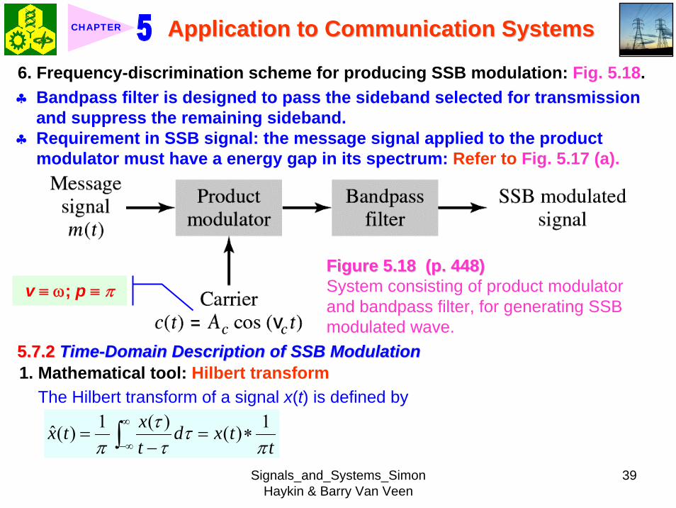
Signals_and_Systems_Simon Haykin amp Barry Van Veen
39
Application to Communication SystemsApplication to Communication SystemsCHAPTER
6 Frequency-discrimination scheme for producing SSB modulation Fig 518clubs Bandpass filter is designed to pass the sideband selected for transmission
and suppress the remaining sidebandclubs Requirement in SSB signal the message signal applied to the product
modulator must have a energy gap in its spectrum Refer to Fig 517 (a)
Figure 518 (p 448)Figure 518 (p 448)System consisting of product modulator and bandpass filter for generating SSB modulated wave
v equiv ω p equiv π
572 572 TimeTime--Domain Description of SSB ModulationDomain Description of SSB Modulation1 Mathematical tool Hilbert transform
The Hilbert transform of a signal x(t) is defined by1 ( ) 1ˆ( ) ( )xx t d x t
t tτ τ
π τ πinfin
minusinfin= = lowast
minusint
Signals_and_Systems_Simon Haykin amp Barry Van Veen
40
Application to Communication SystemsApplication to Communication SystemsCHAPTER
The Fourier transform of 1(πt) is minus j times the signum function denoted
1 for 0sgn( ) 0 for 0
1 for 0
ωω ω
ω
+ gt⎧⎪= =⎨⎪minus lt⎩
2 Passing x(t) through a Hilbert transformer is equivalent to the combination of the following two operations in frequency domain1) Keeping X(jω)unchanged for all ω 2) Shifting areX(jω) (ie the phase spectrum of x(t)) by +90deg for negative
frequencies and minus 90deg for positive frequencies clubs Hilbert transformer = Wideband minus 90deg phase shifter 573 573 Vestigial Sideband ModulationVestigial Sideband Modulation1 When the message signal contains significant components at extremely
low frequencies the upper and lower sidebands meet at the carrier frequency
Using SSB is inappropriateUsing SSB is inappropriateEx TV signals or
wideband dataUsing VSB (Vestigial sideband) modulation is appropriateUsing VSB (Vestigial sideband) modulation is appropriate
Signals_and_Systems_Simon Haykin amp Barry Van Veen
41
Application to Communication SystemsApplication to Communication SystemsCHAPTER
2 VSB is a compromise between SSB and DSB-SC forms of modulationIn VSB modulation one sideband is passes almost completely whereas just a trace or vestige of the other sideband is retained
3 Fig 519 illustrates a VSB modulated wave s(t) in relation to the message signal m(t)
v equiv ω p equiv π
Figure 519 (p 449)Figure 519 (p 449)Spectral content of VSB modulated wave (a) Magnitude spectrum of message signal (c) Magnitude spectrum of VSB modulated wave containing a vestige of the lower sideband
clubs The lower sideband is modified into the vestigial sideband4 Transmission bandwidth of VSB modulated wave T m vω ω ω= + (523)
where ωm is the message bandwidth and ωu is the width of the vestigial sideband
Signals_and_Systems_Simon Haykin amp Barry Van Veen
42
Application to Communication SystemsApplication to Communication SystemsCHAPTER
5 Generation of VSB modulated wave Fig 520
Figure 520 (p 450)Figure 520 (p 450)System consisting of product modulator and sideband shaping filter for generating VSB modulated wave
v equiv ω p equiv π
Passing a DSBPassing a DSB--SC modulated wave through a sidebandSC modulated wave through a sideband--shaping filtershaping filter6 The sideband-shaping filter is designed so that the original message
spectrum M(jω) is reproduced on the demodulation as a result of the superposition of two spectra
1) The positive-frequency part of S(jω) (ie the Fourier transform of the transmitted signal s(t)) shifted downward in frequency by ωc
2) The negative-frequency part of S(jω) shifted upward in frequency by ωc
Fig 521 A reflection of the vestige of the lower sideband makes up for the missing parts of the upper sideband
Signals_and_Systems_Simon Haykin amp Barry Van Veen
43
Application to Communication SystemsApplication to Communication SystemsCHAPTER
Figure 521 (p 450)Figure 521 (p 450)Superposition of the two spectra shown in parts (a) and (b) of the figure results in the original message spectrum (shown dashed) upon demodulation
58 58 PulsePulse--Amplitude Modulation Amplitude Modulation clubs Basic concept
Basic role in the operation of AM Frequency-shiftingBasic role in the operation of PAM Sampling
581 581 Sampling RevisitedSampling Revisited1 Sampling theorem
In view point of PAMIn view point of PAM
Signals_and_Systems_Simon Haykin amp Barry Van Veen
44
Application to Communication SystemsApplication to Communication SystemsCHAPTER
1) A band-limited signal of finite energy that has no radian frequency components higher than ωm is uniquely determined by the values of the signal at instants of time separated by π ωm seconds
2) A band-limited signal of finite energy that has no radian frequency components higher than ωm may be completely recovered from a knowledge of its samples taken at the rate of ωm π per seconds
clubs Part 1) rArr Be exploited in the transmitter of a PAM clubs Part 2) rArr Be exploited in the Receiver of a PAM2 To combat the effects of aliasing in practice we use two corrective measures1) Prior to sampling a low-pass antialiasing filter is used to attenuate those high-
frequency components of the signal which lie outside the band of interest2) The filtered signal is sampled at a rate slightly higher than the Nyquist rate3 Generation of a PAM signal Fig 522Fig 522Example 54 Telephonic CommunicationThe highest frequency component of a speech signal needed for telephonic communication is about 31 kHz Suggest a suitable value for the sampling rate ltltSolgtSolgt
Signals_and_Systems_Simon Haykin amp Barry Van Veen
45
Application to Communication SystemsApplication to Communication SystemsCHAPTER
Figure 522 (p 451)Figure 522 (p 451)System consisting of antialiasing filter and sample-and-hold circuit for converting a message signal into a flattopped PAM signal
1 The highest frequency component of 31 kHz corresponds to 362 10 radsmω π= times
Correspondingly the Nyquist rate is
62 kHzmωπ
=
2 A suitable value for the sampling rate-one slightly higher than the Nyquistrate-may be 8 kHz a rate that is the international standard for telephone speech signals
Signals_and_Systems_Simon Haykin amp Barry Van Veen
46
Application to Communication SystemsApplication to Communication SystemsCHAPTER
582 582 Mathematical Description of PAMMathematical Description of PAM1 The carrier wave used in PAM consists of a sequence of short pulses of
fixed duration in terms of which PAM is formally defined as followsPAM is a form of pulse modulation in which the amplitude of the PAM is a form of pulse modulation in which the amplitude of the pulsed carrier is pulsed carrier is varied in accordance with instantaneous sample values of the mesvaried in accordance with instantaneous sample values of the message signalsage signal the duration of the pulsed carrier is maintained constant throughout
Fig 523Fig 523
Figure 523 (p452) Figure 523 (p452) Waveform of flattopped PAM signal with pulse duration T0 and sampling period Ts
Signals_and_Systems_Simon Haykin amp Barry Van Veen
47
Application to Communication SystemsApplication to Communication SystemsCHAPTER
2 Mathematical representation of the PAM
( ) [ ] ( )sn
s t m n b t nTinfin
=minusinfin
= minussum (524) s(t) equiv PAM signal m(t) equiv
message signal
Ts equiv sampling period m[n] equiv the values of m(t) at t = nTs h(t) equiv rectangular pulse of the unit amplitude and duration T0
3 Rectangular pulse
01 0( )
0 otherwiset T
h tlt lt⎧
= ⎨⎩
(525) Fig 524 (a)Fig 524 (a)
clubs Eq (524) is a sample-and-hold operationAnalogous to zeroAnalogous to zero--orderorder--holdhold--
based reconstruction in Sec 46based reconstruction in Sec 46
差異差異hh((tt) ) 的的TTss與與TT00
4 Impulse-sampled version of message signal m(t)
( ) [ ] ( )sn
m t m n t nTδ δinfin
=minusinfin
= minussum (526)
5 PAM signal( ) [ ] ( )
( ) ( )
sn
s t m n b t nT
m t b tδ
infin
=minusinfin
= minus
=
sum(527)
Convolution of impulse-sampled version mδ(t) and h(t)
Time domain Time domain operationoperation
Signals_and_Systems_Simon Haykin amp Barry Van Veen
48
Application to Communication SystemsApplication to Communication SystemsCHAPTER
Figure 524 (p 453)(a) Rectangular pulse h(t) of unit amplitude and duration T0 (b) Magnitude spectrum |H(jω)| and phase spectrum argH(jω) of pulse h(t)
v equiv ω p equiv π
Signals_and_Systems_Simon Haykin amp Barry Van Veen
49
Application to Communication SystemsApplication to Communication SystemsCHAPTER
6 FT of PAM signal( ) ( ) ( )S j M j H jδω ω ω= (528)
where( ) ( )FTS j s tω larr⎯rarr ( ) ( )FTM j m tδ δω larr⎯rarr ( ) ( )FTH j h tω larr⎯rarr
7 Impulse sampling of the message signal m(t) introduces periodicity into the spectrum as given by
1( ) ( ( ))sks
M j M j kTδ ω ω ω
infin
=minusinfin
= minussum (529) 1Ts equiv sampling rate ωs = 2πTs rads
1( ) ( ( )) ( )sks
S j M j k H jT
ω ω ω ωinfin
=minusinfin
= minussum (530)
( ) ( )FTM j m tω larr⎯rarrwhere
clubs Suppose that m(t) is strictly band limited and that the sampling rate 1Ts is greater than the Nyquist rate Then passing s(t) through a reconstruction filter chosen as an ideal low-pass filter with cutoff frequency ωm and gain Ts we find that the spectrum of the resulting filter output is equal to M(jω)H(jω)
Signals_and_Systems_Simon Haykin amp Barry Van Veen
50
Application to Communication SystemsApplication to Communication SystemsCHAPTER
8 From Eq (525) we find that0 2
0 0( ) sin ( (2 )) j TH j T c T e ωω ω π minus= (531) Fig 524(b) magnitude and phase of H(jω)
clubs Using PAM to represent a continuous-time message signal we introduce amplitude distortion as well as a delay of T02
clubs The frequency distortion caused by the use of flat-topped sampled in the generation of a PAM wave illustrated in Fig 523Fig 523 is referred to as the aperture effect
583 583 Demodulation of PAM SignalDemodulation of PAM Signal1 Reconstruction scheme Fig 525Fig 525
Figure 525 (p 454)Figure 525 (p 454)System consisting of low-pass interpolation filter and equalizer for reconstructing a message signal from its flattopped sampled version
clubs The system consists of low-pass interpolation filter and equalizer connected in cascade
Signals_and_Systems_Simon Haykin amp Barry Van Veen
51
Application to Communication SystemsApplication to Communication SystemsCHAPTER
2 The cutoff frequency of low-pass filter = the highest frequency ωm of message signal
3 The equalizer is used to correct the aperture effect due to flat-topped sampling in the sample-and-hold circuit
4 The equalizer has the effect of decreasing the in-band loss of the interpolation filter as frequency increases in such a manner as to compensate for the aperture effect
5 Amplitude response of equalizer
0
0 0 0 0
1 1 1| ( ) | | sinc( 2) | 2 | sin( 2) |
TH j T T T T
ωω ω ω
= =
Frequency response Eq (531)
Example 55 Equalization for PAM TransmissionThe duty cycle in a PAM signal namely T0 Ts is 10 Evaluate the peak amplification required for equalizationltltSolgtSolgt1 At ωm = π Ts which corresponds to the highest frequency component of the
message signal for a sampling rate equal to the Nyquist rate we find from Eq (531) that the magnitude response of the equalizer at ωm normalized to that at zero frequency is
Signals_and_Systems_Simon Haykin amp Barry Van Veen
52
Application to Communication SystemsApplication to Communication SystemsCHAPTER
Figure 526 (p 455)Figure 526 (p 455)Normalized equalization (to compensate for aperture effect) plotted against the duty cycle T0Ts
Signals_and_Systems_Simon Haykin amp Barry Van Veen
53
Application to Communication SystemsApplication to Communication SystemsCHAPTER
0
0 0
( 2)( )1sin (05 ) sin[( 2)( )]
s
s s
T Tc T T T T
ππ
=
where the ratio T0 Ts is equal to the duty cycle of the sampling pulses 2 In Fig 526Fig 526 this result is plotted as a function of the duty cycle T0 Ts Ideally it
should be equal to unity for all values of T0 Ts 3 For a duty cycle of 10 it is equal to 10041 It follows that for duty cycles of less
than 10 the magnitude equalization required is less than 10041 in which case the aperture effect is usually considered to be negligible
59 59 Multiplexing Multiplexing clubs Three basic types of multiplexing1 Frequency-division multiplexing in which the signals are separated by
allocating them to different frequency bands This is illustrated in Fig 527(a) for the case of six different message signals Frequency-division multiplexing favors the use of CW modulation where each message signal is able to use the channel on a continuous-time basis
2 Time-division multiplexing wherein the signals are separated by allocating them to different time slots within a sampling interval
Signals_and_Systems_Simon Haykin amp Barry Van Veen
54
Application to Communication SystemsApplication to Communication SystemsCHAPTER
This second type of multiplexing is illustrated in Fig 527(b) for the case of six different message signals Code-division multiplexing which relies on the assignment of different codes to the individual users of the channel
3 Code-division multiplexing which relies on the assignment of different codes to the individual users of the channel
591 591 FrequencyFrequency--Domain Multiplexing (FDM)Domain Multiplexing (FDM)1 Block diagram Fig 528Fig 5282 Incoming message signals low-pass variety3 Low-pass filter to remove high-frequency components such that the signal
in each channel does not disturb each other4 MOD (modulator) shift the frequency ranges of the signals so as to occupy
mutually exclusive frequency intervalsSSB is often used in this stageEx Voice input is usually assigned a bandwidth of 4 kHz
5 Band-pass filters are used to restrict the band of each modulated wave to its prescribed range
6 Band-pass filters in receiver separate the message signals7 DEM (demodulator) to recover signalsclubs FDM in Fig 528 operates in only one direction
Signals_and_Systems_Simon Haykin amp Barry Van Veen
55
Application to Communication SystemsApplication to Communication SystemsCHAPTER
Figure 527 (p 456)Figure 527 (p 456)Two basic forms of multiplexing (a) Frequency-division multiplexing (with guardbands) (b) Time-division multiplexing no provision is made here for synchronizing pulses
Signals_and_Systems_Simon Haykin amp Barry Van Veen
56
Application to Communication SystemsApplication to Communication SystemsCHAPTER
Figure 528 (p 457)Figure 528 (p 457)Block diagram of FDM system showing the important constituents of the transmitter and receiver
Signals_and_Systems_Simon Haykin amp Barry Van Veen
57
Application to Communication SystemsApplication to Communication SystemsCHAPTER
Example 56 SSB-FDM System
ltltSolgtSolgt
An FDM system is used to multiplex 24 independent voice signals SSB modulation is used for the transmission Given that each voice signal is allotted a bandwidth 4kHz calculate the overall transmission bandwidth of the channel
With each voice signal allotted a bandwidth of 4 kHz the use of SSB modulation requires a bandwidth of 4 kHz for its transmission Accordingly the overall transmission bandwidth provided by the channel is 24 X 4 = 96 kHz 592 592 TimeTime--Domain Multiplexing (TDM)Domain Multiplexing (TDM)clubs Basic to the operation of a TDM system is the sampling theoremclubs The transmission of the message samples engages the transmission channel for
only a fraction of the sampling interval on a periodic basis equal to the width T0 of a PAM modulating pulse
1 Block diagram Fig 529Fig 5292 Commutator is usually implemented by means of electronic switching
circuitry3 The function of commutator is two folds
Signals_and_Systems_Simon Haykin amp Barry Van Veen
58
Application to Communication SystemsApplication to Communication SystemsCHAPTER
Figure 529 (p 458)Figure 529 (p 458)Block diagram of TDM system showing the important constituents of the transmitter and receiver
(1) To take a narrow sample of each of the M input message signals at a rate 1Tsthat is slightly higher than ωcπ where ωc is the cutoff frequency of the input low-pass filter
(2) To sequentially interleave these M samples inside a sampling interval Ts4 Pulse modulator transform the multiplexed signal into a form suitable for
transmission over the common channel
Signals_and_Systems_Simon Haykin amp Barry Van Veen
59
Application to Communication SystemsApplication to Communication SystemsCHAPTER
clubs The use of time-division multiplexing introduces a bandwidth expansion factor M because the scheme must squeeze M samples derived from M independent message sources into a time slot equal to one sampling interval
5 Pulse demodulator performs the inverse operation of the pulse modulator6 Decommutator distributes the narrow samples produced by pulse demodulator to the appropriate low-pass reconstruction filter7 Synchronization between the timing operations of the transmitter and
receiver in a TDM system is essential for satisfactory performance of the system
Inserting an extra pulse into each sampling interval on a regular basisBandwidth expansion factor is increased to M + 1
clubs The TDM system is hghly sensitive to the dispersion in the common transmission channel
Example 57 Comparison of TDM with FDMATDM system is used to multiplex four independent voice signals using PAM Each voice signal is sampled at the rate of 8 kHz The system incorporates a synchronizing pulse train for its proper operation
Signals_and_Systems_Simon Haykin amp Barry Van Veen
60
Application to Communication SystemsApplication to Communication SystemsCHAPTER
(a) Determine the timing relationships between the synchronizing pulse train and the impulse trains used to sample the four voice signals
(b) Calculate the transmission bandwidth of the channel for the TDM system and compare the result with a corresponding FDM system using SSBmodulation
ltltSolgtSolgt(a) The sampling period is
31 125 s
8 10sT s μ= =times
In this example the number of voice signals is M = 4 Hence dividing the sampling period of 125 μs among these voice signals and the synchronizing pulse train we obtain the time slot allocated to each one of them
0 1125 25 s
5
sTTM
μ
=+
= =
Signals_and_Systems_Simon Haykin amp Barry Van Veen
61
Application to Communication SystemsApplication to Communication SystemsCHAPTER
Figure 530Figure 530 shows the timing relationships between the synchronizing pulse train and the four impulse trains used to sample the different voice signals in a single frame Each frame includes time slots of common duration T0 = 25 μs which are allocated to the pulse-modulated signals and synchronizing pulse
Figure 530 (p 459)Figure 530 (p 459)Composition of one frame of a multiplexed PAM signal incorporating four voice-signals and a synchronizing pulse
Signals_and_Systems_Simon Haykin amp Barry Van Veen
62
Application to Communication SystemsApplication to Communication SystemsCHAPTER
(b) As a consequence of the time-bandwidth product (see Section 317) there is an inverse relationship between the duration of a pulse and the bandwidth (ie cutoff frequency) of the channel needed for itstransmission Accordingly the overall transmission bandwidth of the channel is
0
21 1 MHz 40 kHz
25
TTf
T
ωπ
=
= = =
In contrast the use of an FDM system based on SSB modulation requires a channel bandwidth equal to M times that of a single voice signal-that is 4 X 4 = 16 kHz Thus the use of PAM-TDM requires a channel bandwidth that is 40 16 = 25 times that of SSB-FDMIn practice pulse-code modulation is commonly used as the method of modulation for TDM this results in a further increase in channel bandwidth depending on the length of the code word used in the digital representation of each pulse in the PAM signal
Signals_and_Systems_Simon Haykin amp Barry Van Veen
63
Application to Communication SystemsApplication to Communication SystemsCHAPTER
510 510 Pulse and Group Delays Pulse and Group Delays 1 Whenever a signal is transmitted through a dispersive (ie frequency
selective) system some delay is introduced into the output signal in relation to the input signal
2 The delay is determined by the phase response of the system3 Phase response of a dispersive communication channel
( ) arg ( )H jφ ω ω= (532)
A signal is transmitted through the channel at a frequency ωc The signal received at the channel lags the transmitted signal by φ(ωc) The time delay is called phase delay formally defined as
( )cp
c
φ ωτω
= minus (533)
The phase delay is not necessarily the true signal delayclubs Case study for DSB-SC1 Transmitted signal
0( ) cos( ) cos( )cs t A t tω ω= (534)
ωc equiv carrier frequency ω0 equiv sinusoidal modulation frequency
A = AcA0
Signals_and_Systems_Simon Haykin amp Barry Van Veen
64
Application to Communication SystemsApplication to Communication SystemsCHAPTER
1 21 1( ) cos( ) cos( )2 2
s t A t A tω ω= +
1 0cω ω ω= + (535) where
2 0cω ω ω= minus (536)
Upper frequency
Lower frequency
2 Let the s(t) be transmitted through the channel with phase response φ (ω) Accordingly the signal received at the channel output is
1 1 2 21 1( ) cos( ( )) cos( ( ))2 2
y t A t A tω φ ω ω φ ω= + + +
1 2 1 20
( ) ( ) ( )1 ( )( ) cos cos2 2cy t A t tφ ω φ ω φ ω φ ωω ω+⎛ ⎞ ⎛ ⎞= + +⎜ ⎟ ⎜ ⎟
⎝ ⎠ ⎝ ⎠(537)
3 Two observations from Eq (537)1) The carrier component at frequency ωc in y(t) lags its counterpart in s(t) by
frac12 (φ (ω1) + φ (ω2)) which represents a time delay equal to
1 2 1 2
c 1 2
( )+ ( ) ( )+ ( )2 +
φ ω φ ω φ ω φ ωω ω ω
minus = minus (538)
Signals_and_Systems_Simon Haykin amp Barry Van Veen
65
Application to Communication SystemsApplication to Communication SystemsCHAPTER
2) The message component at frequency ω0 in y(t) lags its counterpart in s(t) by frac12 (φ (ω1) minus φ (ω2)) which represents a time delay equal to
1 2 1 2
0 1 2
( ) ( ) ( ) ( )2
φ ω φ ω φ ω φ ωω ω ωminus minus
minus = minusminus
(539)
4 Suppose that ω0 lt ωc rArr the side frequencies are close together with ω c between them Such a modulated signal is said to be a narrowband signal The phase response φ (ω) in the vicinity of ω = ωc is approximated by two-term Taylor series expansion
( )( ) ( ) ( )c
c cd
d ω ω
φ ωφ ω φ ω ω ωω =
= + times minus (540)
Phase delay = ( ) c cφ ω ωminus
5 The time delay introduced by the message signal (ie he ldquoenveloperdquo of the modulated signal) is given by
( )
c
gd
d ω ω
φ ωτω =
= minus (541) The time delay τg is called the
envelope delay or group delay
Signals_and_Systems_Simon Haykin amp Barry Van Veen
66
Application to Communication SystemsApplication to Communication SystemsCHAPTER
6 When a modulated signal is transmitted through a communication channel there are two different delays to be considered1) The carrier or phase delay τp defined by Eq (533)2) The envelope or group delay τg defined by Eq (541)
clubs The group delay is the true signal delay
Example 58 Phase and Group Delays for Ban-pass Channel
ltltSolgtSolgt
The phase response of a band-pass communication channel is defined by 2 2
1( ) tan c
c
ω ωφ ωωω
minus ⎛ ⎞minus= minus ⎜ ⎟
⎝ ⎠The signal s(t) defined in Eq (534) is transmitted through this channel with
475 radscω = 0 025 radsω =andCalculate (a) the phase delay and (b) the group delay
(a) At ω = ωc φ (ωc) = 0 According to Eq (533) the phase delay τ p is zero (b) Differentiating φ (ω) with respect to ω we get
Signals_and_Systems_Simon Haykin amp Barry Van Veen
67
Application to Communication SystemsApplication to Communication SystemsCHAPTER
2 2
2 2 2 2 2
( )( )( )
c c
c c
dd
ω ω ωφ ωω ω ω ω ω
+= minus
+ minus
Using thing result in Eq (541) we find that the group delay is 2 2 04211
475gc
sτω
= = =
1 One waveform shown as a solid curve was obtained by multiplying the transmitted signal s(t) by the carrier wave cos(ωct)
2 The second waveform shown as a dotted curve was obtained by multiplying the received signal y(t) by the carrier wave cos(ωct)
To display the results obtained in parts (a) and (b) in graphical form Fig 531Fig 531shows a superposition of two waveforms obtained as follows
The figure clearly shows that the carrier (phase) delay τ p is zero and the envelope of the received signal y(t) is lagging behind that of the transmitted signal by τs seconds For the presentation of waveforms in this figure we purposely did not use a filter to suppress the high frequency components resulting from the multiplications described under points 1 and 2 because of the desire to retain a contribution due to the carrier for display
Signals_and_Systems_Simon Haykin amp Barry Van Veen
68
Application to Communication SystemsApplication to Communication SystemsCHAPTER
Figure 531 Figure 531 (p 463)(p 463)Highlighting the zero carrier delay (solid curve) and group delay τg (dotted curve) which are determined in accordance with Example 58
Signals_and_Systems_Simon Haykin amp Barry Van Veen
69
Application to Communication SystemsApplication to Communication SystemsCHAPTER
clubs Not also that the separation between the upper side frequency ω1 = ωc + ω0 = 500 rads and the lower side frequency ω2 = ωc minus ω0 = 450 rads is about 10 of the carrier frequency ωc = 475 rads which justifies referring to the modulated signal in this example as a narrowband signal
5101 5101 Some Practical ConsiderationsSome Practical Considerationsclubs What is the practical importance of group delay 1 Eq (541) for determining group delay applies strictly to narrowband
modulated signal2 The message bandwidth may be comparable to the carrier frequency In
this situation the group delay is formulated as a frequency-dependent parameter ie ( )d( )g d
φ ωτ ωω
= minus (542)
3 When a wideband modulated signals transmitted through a dispersive channel the frequency components of the message signal are delayed by different amounts at the channel output
Delay distortionFig 532Fig 532 Group delay response of voice-grade telephone channel
Signals_and_Systems_Simon Haykin amp Barry Van Veen
70
Application to Communication SystemsApplication to Communication SystemsCHAPTER
Figure 532 (p 464)Group delay response of voice-grade telephone channel (Adapted from J C Bellamy Digital Telephony Wiley 1982)
511 511 Exploring Concepts with MATLABExploring Concepts with MATLAB5111 5111 Full AMFull AMclubs Sinusoidal modulation
clubs To reconstruct a faithful version of the original message signal in the receiver we have to use a delay equalizer
0( ) [1 cos( )]cos( )c cs t A t tμ ω ω= +1 AM experiment
1cA =
08 radscω π= 0 01 radsω π=Carrier amplitude
Carrier frequency Modulation amplitude
Signals_and_Systems_Simon Haykin amp Barry Van Veen
71
Application to Communication SystemsApplication to Communication SystemsCHAPTER
2 We wish to display and analyze 10 full cycles of the AM wave corresponding to a total duration of 200 s Choosing a sampling rate 1Ts = 10 Hz we have a total of N = 2000 time samples The frequency band of interest is minus 10 π ≦ ω ≦ 10 π Since the separation between the carrier and either side frequency is equal to the modulation frequency ω0 = 01 π rads we would like to have a frequency resolution ωr = 001π rads To achieve this resolution we require the following number of frequency samples (see Eq (442))
20 2000001
s
r
M ω πω π
ge = =
3 We therefore choose M = 2000 To approximate the Fourier transform of the AM wave s(t) we may use a 2000-point DTFS The only variable in the AM experiment is the modulation factor μ with respect to which we wish to investigate three different situationsμ = 05 corresponding to under-modulationμ = 10 for which the AM system is on the verge of over-modulationμ = 20 corresponding to over-modulation
Signals_and_Systems_Simon Haykin amp Barry Van Veen
72
Application to Communication SystemsApplication to Communication SystemsCHAPTER
4 MATLAB commandsAc = 1 carrier amplitudewc = 08pi carrier frequencyw0 = 01pi modulation frequencymu = 05 modulation factort = 0011999s = Ac(1 + mucos(w0t))cos(wct)plot(ts)Smag = abs(fftshift(fft(s2000)))2000 Smag denotes the magnitude specturm of the AM wavew = 10[-1000999]2pi2000plot(wSmag)axis ([-30 30 0 08])
5 5 μμ = 05 = 05 case case Fig 533Fig 533μμ = 10 case = 10 case Fig 534Fig 534μμ = 20 case = 20 case Fig 535Fig 535
Discussion see pp 466-469 textbook
Signals_and_Systems_Simon Haykin amp Barry Van Veen
73
Application to Communication SystemsApplication to Communication SystemsCHAPTER
-30 -20 -10 0 10 20 300
02
04
06
0 50 100 150 200-2
-1
0
1
2
2 22 24 26 28 3
02
04
06
(a) Time (s)
Time domain
Frequency domain
(b) Frequency (rads)
Frequency domain
Frequency (rads)
Figure 533 (p 466)Amplitude modulation with 50 modulation (a) AM wave (b) magnitude spectrum of the AM wave and (c) expanded spectrum around the carrier frequency
μμ = 05 = 05 casecase
Signals_and_Systems_Simon Haykin amp Barry Van Veen
74
Application to Communication SystemsApplication to Communication SystemsCHAPTER
Figure 534 (p 467)Figure 534 (p 467)Amplitude modulation with 100 modulation (a) AM wave (b) magnitude spectrum of the AM wave and (c) expanded spectrum around the carrier frequency
Signals_and_Systems_Simon Haykin amp Barry Van Veen
75
Application to Communication SystemsApplication to Communication SystemsCHAPTER
Figure 535 (p 468)Amplitude modulation with 200 modulation (a) AM wave (b) magnitude spectrum of the AM wave and (c) expanded spectrum around the carrier frequency
Signals_and_Systems_Simon Haykin amp Barry Van Veen
76
Application to Communication SystemsApplication to Communication SystemsCHAPTER
5112 5112 DSBDSB--SC ModulationSC Modulation1 Sinusoidal modulation
0 0( ) cos( ) cos( )c cs t A A t tω ω=
2 MATLAB commands
Ac = 1 carrier amplitudewc = 08pi carrier frequency in radsA0 = 1 amplitude of modulating signalw0 = 01pi frequency of modulating signalt = 011999s = AcA0cos(wct)cos(w0t)plot(ts)Smag = abs(fftshift(fft(s2000)))2000w = 10[-1000999]2pi2000plot(wSmag)
3 3 DSBDSB--SC modulated waveSC modulated wave Fig 536Fig 536 Discussion see pp 466-469 textbook
4 Output of the product modulator in Fig 512 (b) with φ = 0
Signals_and_Systems_Simon Haykin amp Barry Van Veen
77
Application to Communication SystemsApplication to Communication SystemsCHAPTER
Figure 536 (p 469)DSB-SC modulation (a) DSB-SC modulated wave (b) magnitude spectrum of the modulated wave and (c) expanded spectrum around the carrier frequency
Signals_and_Systems_Simon Haykin amp Barry Van Veen
78
Application to Communication SystemsApplication to Communication SystemsCHAPTER
( ) ( ) cos( )cv t s t tω=
5 MATLAB commandsgtgt v = scos(wct)
6 Fig 537 (a) waveforms of v(t) Fig 537 (b) magnitude spectrum which readily shows that v(t) consists of the following components1) A sinusoidal component with frequency 01π rads representing the
modulating wave2) A new DSB-SC modulated wave with double carrier frequency of 16π rads
in actuality the side frequencies of this modulated wave are located at 15πand 17π rads
1) The frequency of the modulating wave lies inside the passband of the filter2) The upper and lower side frequencies of the new DSB-SC modulated wave
lie inside the stopband of the filter
Accordingly we may recover the sinusoidal modulating signal by passing v(t) through low-pass filter with the following requirements
Signals_and_Systems_Simon Haykin amp Barry Van Veen
79
Application to Communication SystemsApplication to Communication SystemsCHAPTER
Figure 537 (p 470)Coherent detection of DSB-SC modulated wave (a) and (b) Waveform and magnitude spectrum of signal produced at the output of produce modulator (c) and (d) waveform and magnitude spectrum of low-pass filter output
Signals_and_Systems_Simon Haykin amp Barry Van Veen
80
Application to Communication SystemsApplication to Communication SystemsCHAPTER
The issue of how to design a filter with these requirements will be considered in detail in Chapter 8 For the present it suffices to say that the preceding requirements can be met by using the following MATLAB commands
gtgt [ba] = butter(30025)gtgt output = filter(bav)
The first command produces s special type of filter called a Butterworth filter For the experiment considered here the filter order is 3 and its normalized cutoff frequency of 0025 is calculated as follows
Actual cutoff frequency of filter 025 radsHalf the sampling rate 10 rads
0025
ππ
=
=
The second command computes the filterrsquos output in response to the product modulator output v(t) (We will revisit the design of this filter in Chapter 8) Figure 537(c) displays the waveform of the low-pass filter output this waveform represents a sinusoidal signal of frequency 005 Hz an observation that is confirmed by using the ffr command to approximate the spectrum of the filter output The result of the computation is shown in Fig 537(d)Fig 537(d)
Signals_and_Systems_Simon Haykin amp Barry Van Veen
81
Application to Communication SystemsApplication to Communication SystemsCHAPTER
7 In Fig 538 we explore another aspect of DSB-SC modulation namely the effect of varying the modulation frequency Figure 538(a) shows five cycles of a DSB-SC modulated wave that has the same carrier frequency as that in Fig 536(a) but the modulation frequency has been reduced to 0025 Hz( ie a radian frequency of 005π) Figure 538(b) shows the magnitude spectrum of this second DSB-SC modulated wave and its zoomed-in version is shown in Fig 538(c) Comparing this latter figure with Fig 536(c) we see clearly that decreasing the modulation frequency has the effect of moving the upper and lower side frequencies closer together which is consistent with modulation theory
5113 5113 Phase and Group DelayPhase and Group Delay1 In Example 58 we studied the phase and group delays for a band-pass
channel with phase response 2 2
1( ) tan c
c
ω ωφ ωωω
minus ⎛ ⎞minus= minus ⎜ ⎟
⎝ ⎠2 At ω = ωc the phase delay is τ p = 0 and the group delay is τ s = 04211s One
of the wave forms displayed in Fig 531Fig 531 is
1( ) ( ) cos( )cx t s t tω=
Signals_and_Systems_Simon Haykin amp Barry Van Veen
82
Application to Communication SystemsApplication to Communication SystemsCHAPTER
Figure 538 (p 472)Effect of varying the modulation frequency compared with that in Fig 537 (a) and (b) Waveform and magnitude spectrum of DSB-SC modulated wave with a modulation frequency one-half that used in Fig 536 (c) expanded spectrum around the carrier frequency
Signals_and_Systems_Simon Haykin amp Barry Van Veen
83
Application to Communication SystemsApplication to Communication SystemsCHAPTER
where (see page 461)
1 2( ) [cos( ) cos( )]2As t t tω ω= +
and ω1 = ωc + ω0 and ω2 = ωc - ω0 The waveform shown in the figure as a solid curve is a plot of x1(t) The other waveform also displayed in Fig 531Fig 531 is
2
1 1 2 2
( ) ( ) cos( )
[cos( ( )) cos( ( ))]cos( )2
c
c
x t y t tA t t t
ω
ω φ ω ω φ ω ω
=
= + + +
where the angle φ (ω1) and φ (ω2) are the values of the phase response φ (ω) at ω = ω1 and ω = ω2 respectively The waveform shown as a dotted curve in the figure is a plot of x2(t)
3 The generation of x1(t) and x2(t) in MATLAB is achieved with the following commands with A2 set equal to unity
Signals_and_Systems_Simon Haykin amp Barry Van Veen
84
Application to Communication SystemsApplication to Communication SystemsCHAPTER
wc = 475w0 = 025w1 = wc + w0w2 = wc - w0t = -10 0001 10o1 = -atan((w1^2 - wc^2)(w1wc))o2 = -atan((w2^2 - wc^2)(w2wc))s = cos(w1t) + cos(w2t)y = cos(w1t + o1) + cos(w2t + o2)x1 = scos(478t)x2 = ycos(475t)plot(tx1b)hold on plot(tx2k)hold offxlabel(Time)ylabel(Amplitude)
Note that we have set (A2) = 1 for convenience of presentation The function atan in the first two commands returns the arctangent Note also that the computation of both x1 and x2 involve element-by-element multiplications ndash hence the use of period followed by an asterisk
Signals_and_Systems_Simon Haykin amp Barry Van Veen
85
Application to Communication SystemsApplication to Communication SystemsCHAPTER
Signals_and_Systems_Simon Haykin amp Barry Van Veen
86
Application to Communication SystemsApplication to Communication SystemsCHAPTER
Signals_and_Systems_Simon Haykin amp Barry Van Veen
87
Application to Communication SystemsApplication to Communication SystemsCHAPTER
Signals_and_Systems_Simon Haykin amp Barry Van Veen
40
Application to Communication SystemsApplication to Communication SystemsCHAPTER
The Fourier transform of 1(πt) is minus j times the signum function denoted
1 for 0sgn( ) 0 for 0
1 for 0
ωω ω
ω
+ gt⎧⎪= =⎨⎪minus lt⎩
2 Passing x(t) through a Hilbert transformer is equivalent to the combination of the following two operations in frequency domain1) Keeping X(jω)unchanged for all ω 2) Shifting areX(jω) (ie the phase spectrum of x(t)) by +90deg for negative
frequencies and minus 90deg for positive frequencies clubs Hilbert transformer = Wideband minus 90deg phase shifter 573 573 Vestigial Sideband ModulationVestigial Sideband Modulation1 When the message signal contains significant components at extremely
low frequencies the upper and lower sidebands meet at the carrier frequency
Using SSB is inappropriateUsing SSB is inappropriateEx TV signals or
wideband dataUsing VSB (Vestigial sideband) modulation is appropriateUsing VSB (Vestigial sideband) modulation is appropriate
Signals_and_Systems_Simon Haykin amp Barry Van Veen
41
Application to Communication SystemsApplication to Communication SystemsCHAPTER
2 VSB is a compromise between SSB and DSB-SC forms of modulationIn VSB modulation one sideband is passes almost completely whereas just a trace or vestige of the other sideband is retained
3 Fig 519 illustrates a VSB modulated wave s(t) in relation to the message signal m(t)
v equiv ω p equiv π
Figure 519 (p 449)Figure 519 (p 449)Spectral content of VSB modulated wave (a) Magnitude spectrum of message signal (c) Magnitude spectrum of VSB modulated wave containing a vestige of the lower sideband
clubs The lower sideband is modified into the vestigial sideband4 Transmission bandwidth of VSB modulated wave T m vω ω ω= + (523)
where ωm is the message bandwidth and ωu is the width of the vestigial sideband
Signals_and_Systems_Simon Haykin amp Barry Van Veen
42
Application to Communication SystemsApplication to Communication SystemsCHAPTER
5 Generation of VSB modulated wave Fig 520
Figure 520 (p 450)Figure 520 (p 450)System consisting of product modulator and sideband shaping filter for generating VSB modulated wave
v equiv ω p equiv π
Passing a DSBPassing a DSB--SC modulated wave through a sidebandSC modulated wave through a sideband--shaping filtershaping filter6 The sideband-shaping filter is designed so that the original message
spectrum M(jω) is reproduced on the demodulation as a result of the superposition of two spectra
1) The positive-frequency part of S(jω) (ie the Fourier transform of the transmitted signal s(t)) shifted downward in frequency by ωc
2) The negative-frequency part of S(jω) shifted upward in frequency by ωc
Fig 521 A reflection of the vestige of the lower sideband makes up for the missing parts of the upper sideband
Signals_and_Systems_Simon Haykin amp Barry Van Veen
43
Application to Communication SystemsApplication to Communication SystemsCHAPTER
Figure 521 (p 450)Figure 521 (p 450)Superposition of the two spectra shown in parts (a) and (b) of the figure results in the original message spectrum (shown dashed) upon demodulation
58 58 PulsePulse--Amplitude Modulation Amplitude Modulation clubs Basic concept
Basic role in the operation of AM Frequency-shiftingBasic role in the operation of PAM Sampling
581 581 Sampling RevisitedSampling Revisited1 Sampling theorem
In view point of PAMIn view point of PAM
Signals_and_Systems_Simon Haykin amp Barry Van Veen
44
Application to Communication SystemsApplication to Communication SystemsCHAPTER
1) A band-limited signal of finite energy that has no radian frequency components higher than ωm is uniquely determined by the values of the signal at instants of time separated by π ωm seconds
2) A band-limited signal of finite energy that has no radian frequency components higher than ωm may be completely recovered from a knowledge of its samples taken at the rate of ωm π per seconds
clubs Part 1) rArr Be exploited in the transmitter of a PAM clubs Part 2) rArr Be exploited in the Receiver of a PAM2 To combat the effects of aliasing in practice we use two corrective measures1) Prior to sampling a low-pass antialiasing filter is used to attenuate those high-
frequency components of the signal which lie outside the band of interest2) The filtered signal is sampled at a rate slightly higher than the Nyquist rate3 Generation of a PAM signal Fig 522Fig 522Example 54 Telephonic CommunicationThe highest frequency component of a speech signal needed for telephonic communication is about 31 kHz Suggest a suitable value for the sampling rate ltltSolgtSolgt
Signals_and_Systems_Simon Haykin amp Barry Van Veen
45
Application to Communication SystemsApplication to Communication SystemsCHAPTER
Figure 522 (p 451)Figure 522 (p 451)System consisting of antialiasing filter and sample-and-hold circuit for converting a message signal into a flattopped PAM signal
1 The highest frequency component of 31 kHz corresponds to 362 10 radsmω π= times
Correspondingly the Nyquist rate is
62 kHzmωπ
=
2 A suitable value for the sampling rate-one slightly higher than the Nyquistrate-may be 8 kHz a rate that is the international standard for telephone speech signals
Signals_and_Systems_Simon Haykin amp Barry Van Veen
46
Application to Communication SystemsApplication to Communication SystemsCHAPTER
582 582 Mathematical Description of PAMMathematical Description of PAM1 The carrier wave used in PAM consists of a sequence of short pulses of
fixed duration in terms of which PAM is formally defined as followsPAM is a form of pulse modulation in which the amplitude of the PAM is a form of pulse modulation in which the amplitude of the pulsed carrier is pulsed carrier is varied in accordance with instantaneous sample values of the mesvaried in accordance with instantaneous sample values of the message signalsage signal the duration of the pulsed carrier is maintained constant throughout
Fig 523Fig 523
Figure 523 (p452) Figure 523 (p452) Waveform of flattopped PAM signal with pulse duration T0 and sampling period Ts
Signals_and_Systems_Simon Haykin amp Barry Van Veen
47
Application to Communication SystemsApplication to Communication SystemsCHAPTER
2 Mathematical representation of the PAM
( ) [ ] ( )sn
s t m n b t nTinfin
=minusinfin
= minussum (524) s(t) equiv PAM signal m(t) equiv
message signal
Ts equiv sampling period m[n] equiv the values of m(t) at t = nTs h(t) equiv rectangular pulse of the unit amplitude and duration T0
3 Rectangular pulse
01 0( )
0 otherwiset T
h tlt lt⎧
= ⎨⎩
(525) Fig 524 (a)Fig 524 (a)
clubs Eq (524) is a sample-and-hold operationAnalogous to zeroAnalogous to zero--orderorder--holdhold--
based reconstruction in Sec 46based reconstruction in Sec 46
差異差異hh((tt) ) 的的TTss與與TT00
4 Impulse-sampled version of message signal m(t)
( ) [ ] ( )sn
m t m n t nTδ δinfin
=minusinfin
= minussum (526)
5 PAM signal( ) [ ] ( )
( ) ( )
sn
s t m n b t nT
m t b tδ
infin
=minusinfin
= minus
=
sum(527)
Convolution of impulse-sampled version mδ(t) and h(t)
Time domain Time domain operationoperation
Signals_and_Systems_Simon Haykin amp Barry Van Veen
48
Application to Communication SystemsApplication to Communication SystemsCHAPTER
Figure 524 (p 453)(a) Rectangular pulse h(t) of unit amplitude and duration T0 (b) Magnitude spectrum |H(jω)| and phase spectrum argH(jω) of pulse h(t)
v equiv ω p equiv π
Signals_and_Systems_Simon Haykin amp Barry Van Veen
49
Application to Communication SystemsApplication to Communication SystemsCHAPTER
6 FT of PAM signal( ) ( ) ( )S j M j H jδω ω ω= (528)
where( ) ( )FTS j s tω larr⎯rarr ( ) ( )FTM j m tδ δω larr⎯rarr ( ) ( )FTH j h tω larr⎯rarr
7 Impulse sampling of the message signal m(t) introduces periodicity into the spectrum as given by
1( ) ( ( ))sks
M j M j kTδ ω ω ω
infin
=minusinfin
= minussum (529) 1Ts equiv sampling rate ωs = 2πTs rads
1( ) ( ( )) ( )sks
S j M j k H jT
ω ω ω ωinfin
=minusinfin
= minussum (530)
( ) ( )FTM j m tω larr⎯rarrwhere
clubs Suppose that m(t) is strictly band limited and that the sampling rate 1Ts is greater than the Nyquist rate Then passing s(t) through a reconstruction filter chosen as an ideal low-pass filter with cutoff frequency ωm and gain Ts we find that the spectrum of the resulting filter output is equal to M(jω)H(jω)
Signals_and_Systems_Simon Haykin amp Barry Van Veen
50
Application to Communication SystemsApplication to Communication SystemsCHAPTER
8 From Eq (525) we find that0 2
0 0( ) sin ( (2 )) j TH j T c T e ωω ω π minus= (531) Fig 524(b) magnitude and phase of H(jω)
clubs Using PAM to represent a continuous-time message signal we introduce amplitude distortion as well as a delay of T02
clubs The frequency distortion caused by the use of flat-topped sampled in the generation of a PAM wave illustrated in Fig 523Fig 523 is referred to as the aperture effect
583 583 Demodulation of PAM SignalDemodulation of PAM Signal1 Reconstruction scheme Fig 525Fig 525
Figure 525 (p 454)Figure 525 (p 454)System consisting of low-pass interpolation filter and equalizer for reconstructing a message signal from its flattopped sampled version
clubs The system consists of low-pass interpolation filter and equalizer connected in cascade
Signals_and_Systems_Simon Haykin amp Barry Van Veen
51
Application to Communication SystemsApplication to Communication SystemsCHAPTER
2 The cutoff frequency of low-pass filter = the highest frequency ωm of message signal
3 The equalizer is used to correct the aperture effect due to flat-topped sampling in the sample-and-hold circuit
4 The equalizer has the effect of decreasing the in-band loss of the interpolation filter as frequency increases in such a manner as to compensate for the aperture effect
5 Amplitude response of equalizer
0
0 0 0 0
1 1 1| ( ) | | sinc( 2) | 2 | sin( 2) |
TH j T T T T
ωω ω ω
= =
Frequency response Eq (531)
Example 55 Equalization for PAM TransmissionThe duty cycle in a PAM signal namely T0 Ts is 10 Evaluate the peak amplification required for equalizationltltSolgtSolgt1 At ωm = π Ts which corresponds to the highest frequency component of the
message signal for a sampling rate equal to the Nyquist rate we find from Eq (531) that the magnitude response of the equalizer at ωm normalized to that at zero frequency is
Signals_and_Systems_Simon Haykin amp Barry Van Veen
52
Application to Communication SystemsApplication to Communication SystemsCHAPTER
Figure 526 (p 455)Figure 526 (p 455)Normalized equalization (to compensate for aperture effect) plotted against the duty cycle T0Ts
Signals_and_Systems_Simon Haykin amp Barry Van Veen
53
Application to Communication SystemsApplication to Communication SystemsCHAPTER
0
0 0
( 2)( )1sin (05 ) sin[( 2)( )]
s
s s
T Tc T T T T
ππ
=
where the ratio T0 Ts is equal to the duty cycle of the sampling pulses 2 In Fig 526Fig 526 this result is plotted as a function of the duty cycle T0 Ts Ideally it
should be equal to unity for all values of T0 Ts 3 For a duty cycle of 10 it is equal to 10041 It follows that for duty cycles of less
than 10 the magnitude equalization required is less than 10041 in which case the aperture effect is usually considered to be negligible
59 59 Multiplexing Multiplexing clubs Three basic types of multiplexing1 Frequency-division multiplexing in which the signals are separated by
allocating them to different frequency bands This is illustrated in Fig 527(a) for the case of six different message signals Frequency-division multiplexing favors the use of CW modulation where each message signal is able to use the channel on a continuous-time basis
2 Time-division multiplexing wherein the signals are separated by allocating them to different time slots within a sampling interval
Signals_and_Systems_Simon Haykin amp Barry Van Veen
54
Application to Communication SystemsApplication to Communication SystemsCHAPTER
This second type of multiplexing is illustrated in Fig 527(b) for the case of six different message signals Code-division multiplexing which relies on the assignment of different codes to the individual users of the channel
3 Code-division multiplexing which relies on the assignment of different codes to the individual users of the channel
591 591 FrequencyFrequency--Domain Multiplexing (FDM)Domain Multiplexing (FDM)1 Block diagram Fig 528Fig 5282 Incoming message signals low-pass variety3 Low-pass filter to remove high-frequency components such that the signal
in each channel does not disturb each other4 MOD (modulator) shift the frequency ranges of the signals so as to occupy
mutually exclusive frequency intervalsSSB is often used in this stageEx Voice input is usually assigned a bandwidth of 4 kHz
5 Band-pass filters are used to restrict the band of each modulated wave to its prescribed range
6 Band-pass filters in receiver separate the message signals7 DEM (demodulator) to recover signalsclubs FDM in Fig 528 operates in only one direction
Signals_and_Systems_Simon Haykin amp Barry Van Veen
55
Application to Communication SystemsApplication to Communication SystemsCHAPTER
Figure 527 (p 456)Figure 527 (p 456)Two basic forms of multiplexing (a) Frequency-division multiplexing (with guardbands) (b) Time-division multiplexing no provision is made here for synchronizing pulses
Signals_and_Systems_Simon Haykin amp Barry Van Veen
56
Application to Communication SystemsApplication to Communication SystemsCHAPTER
Figure 528 (p 457)Figure 528 (p 457)Block diagram of FDM system showing the important constituents of the transmitter and receiver
Signals_and_Systems_Simon Haykin amp Barry Van Veen
57
Application to Communication SystemsApplication to Communication SystemsCHAPTER
Example 56 SSB-FDM System
ltltSolgtSolgt
An FDM system is used to multiplex 24 independent voice signals SSB modulation is used for the transmission Given that each voice signal is allotted a bandwidth 4kHz calculate the overall transmission bandwidth of the channel
With each voice signal allotted a bandwidth of 4 kHz the use of SSB modulation requires a bandwidth of 4 kHz for its transmission Accordingly the overall transmission bandwidth provided by the channel is 24 X 4 = 96 kHz 592 592 TimeTime--Domain Multiplexing (TDM)Domain Multiplexing (TDM)clubs Basic to the operation of a TDM system is the sampling theoremclubs The transmission of the message samples engages the transmission channel for
only a fraction of the sampling interval on a periodic basis equal to the width T0 of a PAM modulating pulse
1 Block diagram Fig 529Fig 5292 Commutator is usually implemented by means of electronic switching
circuitry3 The function of commutator is two folds
Signals_and_Systems_Simon Haykin amp Barry Van Veen
58
Application to Communication SystemsApplication to Communication SystemsCHAPTER
Figure 529 (p 458)Figure 529 (p 458)Block diagram of TDM system showing the important constituents of the transmitter and receiver
(1) To take a narrow sample of each of the M input message signals at a rate 1Tsthat is slightly higher than ωcπ where ωc is the cutoff frequency of the input low-pass filter
(2) To sequentially interleave these M samples inside a sampling interval Ts4 Pulse modulator transform the multiplexed signal into a form suitable for
transmission over the common channel
Signals_and_Systems_Simon Haykin amp Barry Van Veen
59
Application to Communication SystemsApplication to Communication SystemsCHAPTER
clubs The use of time-division multiplexing introduces a bandwidth expansion factor M because the scheme must squeeze M samples derived from M independent message sources into a time slot equal to one sampling interval
5 Pulse demodulator performs the inverse operation of the pulse modulator6 Decommutator distributes the narrow samples produced by pulse demodulator to the appropriate low-pass reconstruction filter7 Synchronization between the timing operations of the transmitter and
receiver in a TDM system is essential for satisfactory performance of the system
Inserting an extra pulse into each sampling interval on a regular basisBandwidth expansion factor is increased to M + 1
clubs The TDM system is hghly sensitive to the dispersion in the common transmission channel
Example 57 Comparison of TDM with FDMATDM system is used to multiplex four independent voice signals using PAM Each voice signal is sampled at the rate of 8 kHz The system incorporates a synchronizing pulse train for its proper operation
Signals_and_Systems_Simon Haykin amp Barry Van Veen
60
Application to Communication SystemsApplication to Communication SystemsCHAPTER
(a) Determine the timing relationships between the synchronizing pulse train and the impulse trains used to sample the four voice signals
(b) Calculate the transmission bandwidth of the channel for the TDM system and compare the result with a corresponding FDM system using SSBmodulation
ltltSolgtSolgt(a) The sampling period is
31 125 s
8 10sT s μ= =times
In this example the number of voice signals is M = 4 Hence dividing the sampling period of 125 μs among these voice signals and the synchronizing pulse train we obtain the time slot allocated to each one of them
0 1125 25 s
5
sTTM
μ
=+
= =
Signals_and_Systems_Simon Haykin amp Barry Van Veen
61
Application to Communication SystemsApplication to Communication SystemsCHAPTER
Figure 530Figure 530 shows the timing relationships between the synchronizing pulse train and the four impulse trains used to sample the different voice signals in a single frame Each frame includes time slots of common duration T0 = 25 μs which are allocated to the pulse-modulated signals and synchronizing pulse
Figure 530 (p 459)Figure 530 (p 459)Composition of one frame of a multiplexed PAM signal incorporating four voice-signals and a synchronizing pulse
Signals_and_Systems_Simon Haykin amp Barry Van Veen
62
Application to Communication SystemsApplication to Communication SystemsCHAPTER
(b) As a consequence of the time-bandwidth product (see Section 317) there is an inverse relationship between the duration of a pulse and the bandwidth (ie cutoff frequency) of the channel needed for itstransmission Accordingly the overall transmission bandwidth of the channel is
0
21 1 MHz 40 kHz
25
TTf
T
ωπ
=
= = =
In contrast the use of an FDM system based on SSB modulation requires a channel bandwidth equal to M times that of a single voice signal-that is 4 X 4 = 16 kHz Thus the use of PAM-TDM requires a channel bandwidth that is 40 16 = 25 times that of SSB-FDMIn practice pulse-code modulation is commonly used as the method of modulation for TDM this results in a further increase in channel bandwidth depending on the length of the code word used in the digital representation of each pulse in the PAM signal
Signals_and_Systems_Simon Haykin amp Barry Van Veen
63
Application to Communication SystemsApplication to Communication SystemsCHAPTER
510 510 Pulse and Group Delays Pulse and Group Delays 1 Whenever a signal is transmitted through a dispersive (ie frequency
selective) system some delay is introduced into the output signal in relation to the input signal
2 The delay is determined by the phase response of the system3 Phase response of a dispersive communication channel
( ) arg ( )H jφ ω ω= (532)
A signal is transmitted through the channel at a frequency ωc The signal received at the channel lags the transmitted signal by φ(ωc) The time delay is called phase delay formally defined as
( )cp
c
φ ωτω
= minus (533)
The phase delay is not necessarily the true signal delayclubs Case study for DSB-SC1 Transmitted signal
0( ) cos( ) cos( )cs t A t tω ω= (534)
ωc equiv carrier frequency ω0 equiv sinusoidal modulation frequency
A = AcA0
Signals_and_Systems_Simon Haykin amp Barry Van Veen
64
Application to Communication SystemsApplication to Communication SystemsCHAPTER
1 21 1( ) cos( ) cos( )2 2
s t A t A tω ω= +
1 0cω ω ω= + (535) where
2 0cω ω ω= minus (536)
Upper frequency
Lower frequency
2 Let the s(t) be transmitted through the channel with phase response φ (ω) Accordingly the signal received at the channel output is
1 1 2 21 1( ) cos( ( )) cos( ( ))2 2
y t A t A tω φ ω ω φ ω= + + +
1 2 1 20
( ) ( ) ( )1 ( )( ) cos cos2 2cy t A t tφ ω φ ω φ ω φ ωω ω+⎛ ⎞ ⎛ ⎞= + +⎜ ⎟ ⎜ ⎟
⎝ ⎠ ⎝ ⎠(537)
3 Two observations from Eq (537)1) The carrier component at frequency ωc in y(t) lags its counterpart in s(t) by
frac12 (φ (ω1) + φ (ω2)) which represents a time delay equal to
1 2 1 2
c 1 2
( )+ ( ) ( )+ ( )2 +
φ ω φ ω φ ω φ ωω ω ω
minus = minus (538)
Signals_and_Systems_Simon Haykin amp Barry Van Veen
65
Application to Communication SystemsApplication to Communication SystemsCHAPTER
2) The message component at frequency ω0 in y(t) lags its counterpart in s(t) by frac12 (φ (ω1) minus φ (ω2)) which represents a time delay equal to
1 2 1 2
0 1 2
( ) ( ) ( ) ( )2
φ ω φ ω φ ω φ ωω ω ωminus minus
minus = minusminus
(539)
4 Suppose that ω0 lt ωc rArr the side frequencies are close together with ω c between them Such a modulated signal is said to be a narrowband signal The phase response φ (ω) in the vicinity of ω = ωc is approximated by two-term Taylor series expansion
( )( ) ( ) ( )c
c cd
d ω ω
φ ωφ ω φ ω ω ωω =
= + times minus (540)
Phase delay = ( ) c cφ ω ωminus
5 The time delay introduced by the message signal (ie he ldquoenveloperdquo of the modulated signal) is given by
( )
c
gd
d ω ω
φ ωτω =
= minus (541) The time delay τg is called the
envelope delay or group delay
Signals_and_Systems_Simon Haykin amp Barry Van Veen
66
Application to Communication SystemsApplication to Communication SystemsCHAPTER
6 When a modulated signal is transmitted through a communication channel there are two different delays to be considered1) The carrier or phase delay τp defined by Eq (533)2) The envelope or group delay τg defined by Eq (541)
clubs The group delay is the true signal delay
Example 58 Phase and Group Delays for Ban-pass Channel
ltltSolgtSolgt
The phase response of a band-pass communication channel is defined by 2 2
1( ) tan c
c
ω ωφ ωωω
minus ⎛ ⎞minus= minus ⎜ ⎟
⎝ ⎠The signal s(t) defined in Eq (534) is transmitted through this channel with
475 radscω = 0 025 radsω =andCalculate (a) the phase delay and (b) the group delay
(a) At ω = ωc φ (ωc) = 0 According to Eq (533) the phase delay τ p is zero (b) Differentiating φ (ω) with respect to ω we get
Signals_and_Systems_Simon Haykin amp Barry Van Veen
67
Application to Communication SystemsApplication to Communication SystemsCHAPTER
2 2
2 2 2 2 2
( )( )( )
c c
c c
dd
ω ω ωφ ωω ω ω ω ω
+= minus
+ minus
Using thing result in Eq (541) we find that the group delay is 2 2 04211
475gc
sτω
= = =
1 One waveform shown as a solid curve was obtained by multiplying the transmitted signal s(t) by the carrier wave cos(ωct)
2 The second waveform shown as a dotted curve was obtained by multiplying the received signal y(t) by the carrier wave cos(ωct)
To display the results obtained in parts (a) and (b) in graphical form Fig 531Fig 531shows a superposition of two waveforms obtained as follows
The figure clearly shows that the carrier (phase) delay τ p is zero and the envelope of the received signal y(t) is lagging behind that of the transmitted signal by τs seconds For the presentation of waveforms in this figure we purposely did not use a filter to suppress the high frequency components resulting from the multiplications described under points 1 and 2 because of the desire to retain a contribution due to the carrier for display
Signals_and_Systems_Simon Haykin amp Barry Van Veen
68
Application to Communication SystemsApplication to Communication SystemsCHAPTER
Figure 531 Figure 531 (p 463)(p 463)Highlighting the zero carrier delay (solid curve) and group delay τg (dotted curve) which are determined in accordance with Example 58
Signals_and_Systems_Simon Haykin amp Barry Van Veen
69
Application to Communication SystemsApplication to Communication SystemsCHAPTER
clubs Not also that the separation between the upper side frequency ω1 = ωc + ω0 = 500 rads and the lower side frequency ω2 = ωc minus ω0 = 450 rads is about 10 of the carrier frequency ωc = 475 rads which justifies referring to the modulated signal in this example as a narrowband signal
5101 5101 Some Practical ConsiderationsSome Practical Considerationsclubs What is the practical importance of group delay 1 Eq (541) for determining group delay applies strictly to narrowband
modulated signal2 The message bandwidth may be comparable to the carrier frequency In
this situation the group delay is formulated as a frequency-dependent parameter ie ( )d( )g d
φ ωτ ωω
= minus (542)
3 When a wideband modulated signals transmitted through a dispersive channel the frequency components of the message signal are delayed by different amounts at the channel output
Delay distortionFig 532Fig 532 Group delay response of voice-grade telephone channel
Signals_and_Systems_Simon Haykin amp Barry Van Veen
70
Application to Communication SystemsApplication to Communication SystemsCHAPTER
Figure 532 (p 464)Group delay response of voice-grade telephone channel (Adapted from J C Bellamy Digital Telephony Wiley 1982)
511 511 Exploring Concepts with MATLABExploring Concepts with MATLAB5111 5111 Full AMFull AMclubs Sinusoidal modulation
clubs To reconstruct a faithful version of the original message signal in the receiver we have to use a delay equalizer
0( ) [1 cos( )]cos( )c cs t A t tμ ω ω= +1 AM experiment
1cA =
08 radscω π= 0 01 radsω π=Carrier amplitude
Carrier frequency Modulation amplitude
Signals_and_Systems_Simon Haykin amp Barry Van Veen
71
Application to Communication SystemsApplication to Communication SystemsCHAPTER
2 We wish to display and analyze 10 full cycles of the AM wave corresponding to a total duration of 200 s Choosing a sampling rate 1Ts = 10 Hz we have a total of N = 2000 time samples The frequency band of interest is minus 10 π ≦ ω ≦ 10 π Since the separation between the carrier and either side frequency is equal to the modulation frequency ω0 = 01 π rads we would like to have a frequency resolution ωr = 001π rads To achieve this resolution we require the following number of frequency samples (see Eq (442))
20 2000001
s
r
M ω πω π
ge = =
3 We therefore choose M = 2000 To approximate the Fourier transform of the AM wave s(t) we may use a 2000-point DTFS The only variable in the AM experiment is the modulation factor μ with respect to which we wish to investigate three different situationsμ = 05 corresponding to under-modulationμ = 10 for which the AM system is on the verge of over-modulationμ = 20 corresponding to over-modulation
Signals_and_Systems_Simon Haykin amp Barry Van Veen
72
Application to Communication SystemsApplication to Communication SystemsCHAPTER
4 MATLAB commandsAc = 1 carrier amplitudewc = 08pi carrier frequencyw0 = 01pi modulation frequencymu = 05 modulation factort = 0011999s = Ac(1 + mucos(w0t))cos(wct)plot(ts)Smag = abs(fftshift(fft(s2000)))2000 Smag denotes the magnitude specturm of the AM wavew = 10[-1000999]2pi2000plot(wSmag)axis ([-30 30 0 08])
5 5 μμ = 05 = 05 case case Fig 533Fig 533μμ = 10 case = 10 case Fig 534Fig 534μμ = 20 case = 20 case Fig 535Fig 535
Discussion see pp 466-469 textbook
Signals_and_Systems_Simon Haykin amp Barry Van Veen
73
Application to Communication SystemsApplication to Communication SystemsCHAPTER
-30 -20 -10 0 10 20 300
02
04
06
0 50 100 150 200-2
-1
0
1
2
2 22 24 26 28 3
02
04
06
(a) Time (s)
Time domain
Frequency domain
(b) Frequency (rads)
Frequency domain
Frequency (rads)
Figure 533 (p 466)Amplitude modulation with 50 modulation (a) AM wave (b) magnitude spectrum of the AM wave and (c) expanded spectrum around the carrier frequency
μμ = 05 = 05 casecase
Signals_and_Systems_Simon Haykin amp Barry Van Veen
74
Application to Communication SystemsApplication to Communication SystemsCHAPTER
Figure 534 (p 467)Figure 534 (p 467)Amplitude modulation with 100 modulation (a) AM wave (b) magnitude spectrum of the AM wave and (c) expanded spectrum around the carrier frequency
Signals_and_Systems_Simon Haykin amp Barry Van Veen
75
Application to Communication SystemsApplication to Communication SystemsCHAPTER
Figure 535 (p 468)Amplitude modulation with 200 modulation (a) AM wave (b) magnitude spectrum of the AM wave and (c) expanded spectrum around the carrier frequency
Signals_and_Systems_Simon Haykin amp Barry Van Veen
76
Application to Communication SystemsApplication to Communication SystemsCHAPTER
5112 5112 DSBDSB--SC ModulationSC Modulation1 Sinusoidal modulation
0 0( ) cos( ) cos( )c cs t A A t tω ω=
2 MATLAB commands
Ac = 1 carrier amplitudewc = 08pi carrier frequency in radsA0 = 1 amplitude of modulating signalw0 = 01pi frequency of modulating signalt = 011999s = AcA0cos(wct)cos(w0t)plot(ts)Smag = abs(fftshift(fft(s2000)))2000w = 10[-1000999]2pi2000plot(wSmag)
3 3 DSBDSB--SC modulated waveSC modulated wave Fig 536Fig 536 Discussion see pp 466-469 textbook
4 Output of the product modulator in Fig 512 (b) with φ = 0
Signals_and_Systems_Simon Haykin amp Barry Van Veen
77
Application to Communication SystemsApplication to Communication SystemsCHAPTER
Figure 536 (p 469)DSB-SC modulation (a) DSB-SC modulated wave (b) magnitude spectrum of the modulated wave and (c) expanded spectrum around the carrier frequency
Signals_and_Systems_Simon Haykin amp Barry Van Veen
78
Application to Communication SystemsApplication to Communication SystemsCHAPTER
( ) ( ) cos( )cv t s t tω=
5 MATLAB commandsgtgt v = scos(wct)
6 Fig 537 (a) waveforms of v(t) Fig 537 (b) magnitude spectrum which readily shows that v(t) consists of the following components1) A sinusoidal component with frequency 01π rads representing the
modulating wave2) A new DSB-SC modulated wave with double carrier frequency of 16π rads
in actuality the side frequencies of this modulated wave are located at 15πand 17π rads
1) The frequency of the modulating wave lies inside the passband of the filter2) The upper and lower side frequencies of the new DSB-SC modulated wave
lie inside the stopband of the filter
Accordingly we may recover the sinusoidal modulating signal by passing v(t) through low-pass filter with the following requirements
Signals_and_Systems_Simon Haykin amp Barry Van Veen
79
Application to Communication SystemsApplication to Communication SystemsCHAPTER
Figure 537 (p 470)Coherent detection of DSB-SC modulated wave (a) and (b) Waveform and magnitude spectrum of signal produced at the output of produce modulator (c) and (d) waveform and magnitude spectrum of low-pass filter output
Signals_and_Systems_Simon Haykin amp Barry Van Veen
80
Application to Communication SystemsApplication to Communication SystemsCHAPTER
The issue of how to design a filter with these requirements will be considered in detail in Chapter 8 For the present it suffices to say that the preceding requirements can be met by using the following MATLAB commands
gtgt [ba] = butter(30025)gtgt output = filter(bav)
The first command produces s special type of filter called a Butterworth filter For the experiment considered here the filter order is 3 and its normalized cutoff frequency of 0025 is calculated as follows
Actual cutoff frequency of filter 025 radsHalf the sampling rate 10 rads
0025
ππ
=
=
The second command computes the filterrsquos output in response to the product modulator output v(t) (We will revisit the design of this filter in Chapter 8) Figure 537(c) displays the waveform of the low-pass filter output this waveform represents a sinusoidal signal of frequency 005 Hz an observation that is confirmed by using the ffr command to approximate the spectrum of the filter output The result of the computation is shown in Fig 537(d)Fig 537(d)
Signals_and_Systems_Simon Haykin amp Barry Van Veen
81
Application to Communication SystemsApplication to Communication SystemsCHAPTER
7 In Fig 538 we explore another aspect of DSB-SC modulation namely the effect of varying the modulation frequency Figure 538(a) shows five cycles of a DSB-SC modulated wave that has the same carrier frequency as that in Fig 536(a) but the modulation frequency has been reduced to 0025 Hz( ie a radian frequency of 005π) Figure 538(b) shows the magnitude spectrum of this second DSB-SC modulated wave and its zoomed-in version is shown in Fig 538(c) Comparing this latter figure with Fig 536(c) we see clearly that decreasing the modulation frequency has the effect of moving the upper and lower side frequencies closer together which is consistent with modulation theory
5113 5113 Phase and Group DelayPhase and Group Delay1 In Example 58 we studied the phase and group delays for a band-pass
channel with phase response 2 2
1( ) tan c
c
ω ωφ ωωω
minus ⎛ ⎞minus= minus ⎜ ⎟
⎝ ⎠2 At ω = ωc the phase delay is τ p = 0 and the group delay is τ s = 04211s One
of the wave forms displayed in Fig 531Fig 531 is
1( ) ( ) cos( )cx t s t tω=
Signals_and_Systems_Simon Haykin amp Barry Van Veen
82
Application to Communication SystemsApplication to Communication SystemsCHAPTER
Figure 538 (p 472)Effect of varying the modulation frequency compared with that in Fig 537 (a) and (b) Waveform and magnitude spectrum of DSB-SC modulated wave with a modulation frequency one-half that used in Fig 536 (c) expanded spectrum around the carrier frequency
Signals_and_Systems_Simon Haykin amp Barry Van Veen
83
Application to Communication SystemsApplication to Communication SystemsCHAPTER
where (see page 461)
1 2( ) [cos( ) cos( )]2As t t tω ω= +
and ω1 = ωc + ω0 and ω2 = ωc - ω0 The waveform shown in the figure as a solid curve is a plot of x1(t) The other waveform also displayed in Fig 531Fig 531 is
2
1 1 2 2
( ) ( ) cos( )
[cos( ( )) cos( ( ))]cos( )2
c
c
x t y t tA t t t
ω
ω φ ω ω φ ω ω
=
= + + +
where the angle φ (ω1) and φ (ω2) are the values of the phase response φ (ω) at ω = ω1 and ω = ω2 respectively The waveform shown as a dotted curve in the figure is a plot of x2(t)
3 The generation of x1(t) and x2(t) in MATLAB is achieved with the following commands with A2 set equal to unity
Signals_and_Systems_Simon Haykin amp Barry Van Veen
84
Application to Communication SystemsApplication to Communication SystemsCHAPTER
wc = 475w0 = 025w1 = wc + w0w2 = wc - w0t = -10 0001 10o1 = -atan((w1^2 - wc^2)(w1wc))o2 = -atan((w2^2 - wc^2)(w2wc))s = cos(w1t) + cos(w2t)y = cos(w1t + o1) + cos(w2t + o2)x1 = scos(478t)x2 = ycos(475t)plot(tx1b)hold on plot(tx2k)hold offxlabel(Time)ylabel(Amplitude)
Note that we have set (A2) = 1 for convenience of presentation The function atan in the first two commands returns the arctangent Note also that the computation of both x1 and x2 involve element-by-element multiplications ndash hence the use of period followed by an asterisk
Signals_and_Systems_Simon Haykin amp Barry Van Veen
85
Application to Communication SystemsApplication to Communication SystemsCHAPTER
Signals_and_Systems_Simon Haykin amp Barry Van Veen
86
Application to Communication SystemsApplication to Communication SystemsCHAPTER
Signals_and_Systems_Simon Haykin amp Barry Van Veen
87
Application to Communication SystemsApplication to Communication SystemsCHAPTER
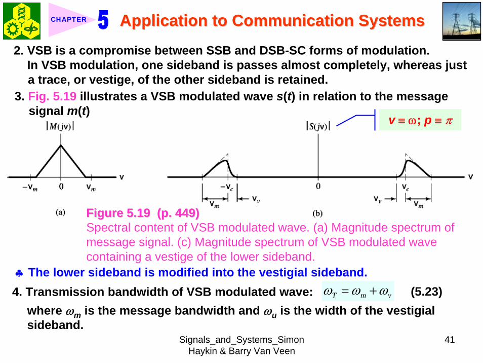
Signals_and_Systems_Simon Haykin amp Barry Van Veen
41
Application to Communication SystemsApplication to Communication SystemsCHAPTER
2 VSB is a compromise between SSB and DSB-SC forms of modulationIn VSB modulation one sideband is passes almost completely whereas just a trace or vestige of the other sideband is retained
3 Fig 519 illustrates a VSB modulated wave s(t) in relation to the message signal m(t)
v equiv ω p equiv π
Figure 519 (p 449)Figure 519 (p 449)Spectral content of VSB modulated wave (a) Magnitude spectrum of message signal (c) Magnitude spectrum of VSB modulated wave containing a vestige of the lower sideband
clubs The lower sideband is modified into the vestigial sideband4 Transmission bandwidth of VSB modulated wave T m vω ω ω= + (523)
where ωm is the message bandwidth and ωu is the width of the vestigial sideband
Signals_and_Systems_Simon Haykin amp Barry Van Veen
42
Application to Communication SystemsApplication to Communication SystemsCHAPTER
5 Generation of VSB modulated wave Fig 520
Figure 520 (p 450)Figure 520 (p 450)System consisting of product modulator and sideband shaping filter for generating VSB modulated wave
v equiv ω p equiv π
Passing a DSBPassing a DSB--SC modulated wave through a sidebandSC modulated wave through a sideband--shaping filtershaping filter6 The sideband-shaping filter is designed so that the original message
spectrum M(jω) is reproduced on the demodulation as a result of the superposition of two spectra
1) The positive-frequency part of S(jω) (ie the Fourier transform of the transmitted signal s(t)) shifted downward in frequency by ωc
2) The negative-frequency part of S(jω) shifted upward in frequency by ωc
Fig 521 A reflection of the vestige of the lower sideband makes up for the missing parts of the upper sideband
Signals_and_Systems_Simon Haykin amp Barry Van Veen
43
Application to Communication SystemsApplication to Communication SystemsCHAPTER
Figure 521 (p 450)Figure 521 (p 450)Superposition of the two spectra shown in parts (a) and (b) of the figure results in the original message spectrum (shown dashed) upon demodulation
58 58 PulsePulse--Amplitude Modulation Amplitude Modulation clubs Basic concept
Basic role in the operation of AM Frequency-shiftingBasic role in the operation of PAM Sampling
581 581 Sampling RevisitedSampling Revisited1 Sampling theorem
In view point of PAMIn view point of PAM
Signals_and_Systems_Simon Haykin amp Barry Van Veen
44
Application to Communication SystemsApplication to Communication SystemsCHAPTER
1) A band-limited signal of finite energy that has no radian frequency components higher than ωm is uniquely determined by the values of the signal at instants of time separated by π ωm seconds
2) A band-limited signal of finite energy that has no radian frequency components higher than ωm may be completely recovered from a knowledge of its samples taken at the rate of ωm π per seconds
clubs Part 1) rArr Be exploited in the transmitter of a PAM clubs Part 2) rArr Be exploited in the Receiver of a PAM2 To combat the effects of aliasing in practice we use two corrective measures1) Prior to sampling a low-pass antialiasing filter is used to attenuate those high-
frequency components of the signal which lie outside the band of interest2) The filtered signal is sampled at a rate slightly higher than the Nyquist rate3 Generation of a PAM signal Fig 522Fig 522Example 54 Telephonic CommunicationThe highest frequency component of a speech signal needed for telephonic communication is about 31 kHz Suggest a suitable value for the sampling rate ltltSolgtSolgt
Signals_and_Systems_Simon Haykin amp Barry Van Veen
45
Application to Communication SystemsApplication to Communication SystemsCHAPTER
Figure 522 (p 451)Figure 522 (p 451)System consisting of antialiasing filter and sample-and-hold circuit for converting a message signal into a flattopped PAM signal
1 The highest frequency component of 31 kHz corresponds to 362 10 radsmω π= times
Correspondingly the Nyquist rate is
62 kHzmωπ
=
2 A suitable value for the sampling rate-one slightly higher than the Nyquistrate-may be 8 kHz a rate that is the international standard for telephone speech signals
Signals_and_Systems_Simon Haykin amp Barry Van Veen
46
Application to Communication SystemsApplication to Communication SystemsCHAPTER
582 582 Mathematical Description of PAMMathematical Description of PAM1 The carrier wave used in PAM consists of a sequence of short pulses of
fixed duration in terms of which PAM is formally defined as followsPAM is a form of pulse modulation in which the amplitude of the PAM is a form of pulse modulation in which the amplitude of the pulsed carrier is pulsed carrier is varied in accordance with instantaneous sample values of the mesvaried in accordance with instantaneous sample values of the message signalsage signal the duration of the pulsed carrier is maintained constant throughout
Fig 523Fig 523
Figure 523 (p452) Figure 523 (p452) Waveform of flattopped PAM signal with pulse duration T0 and sampling period Ts
Signals_and_Systems_Simon Haykin amp Barry Van Veen
47
Application to Communication SystemsApplication to Communication SystemsCHAPTER
2 Mathematical representation of the PAM
( ) [ ] ( )sn
s t m n b t nTinfin
=minusinfin
= minussum (524) s(t) equiv PAM signal m(t) equiv
message signal
Ts equiv sampling period m[n] equiv the values of m(t) at t = nTs h(t) equiv rectangular pulse of the unit amplitude and duration T0
3 Rectangular pulse
01 0( )
0 otherwiset T
h tlt lt⎧
= ⎨⎩
(525) Fig 524 (a)Fig 524 (a)
clubs Eq (524) is a sample-and-hold operationAnalogous to zeroAnalogous to zero--orderorder--holdhold--
based reconstruction in Sec 46based reconstruction in Sec 46
差異差異hh((tt) ) 的的TTss與與TT00
4 Impulse-sampled version of message signal m(t)
( ) [ ] ( )sn
m t m n t nTδ δinfin
=minusinfin
= minussum (526)
5 PAM signal( ) [ ] ( )
( ) ( )
sn
s t m n b t nT
m t b tδ
infin
=minusinfin
= minus
=
sum(527)
Convolution of impulse-sampled version mδ(t) and h(t)
Time domain Time domain operationoperation
Signals_and_Systems_Simon Haykin amp Barry Van Veen
48
Application to Communication SystemsApplication to Communication SystemsCHAPTER
Figure 524 (p 453)(a) Rectangular pulse h(t) of unit amplitude and duration T0 (b) Magnitude spectrum |H(jω)| and phase spectrum argH(jω) of pulse h(t)
v equiv ω p equiv π
Signals_and_Systems_Simon Haykin amp Barry Van Veen
49
Application to Communication SystemsApplication to Communication SystemsCHAPTER
6 FT of PAM signal( ) ( ) ( )S j M j H jδω ω ω= (528)
where( ) ( )FTS j s tω larr⎯rarr ( ) ( )FTM j m tδ δω larr⎯rarr ( ) ( )FTH j h tω larr⎯rarr
7 Impulse sampling of the message signal m(t) introduces periodicity into the spectrum as given by
1( ) ( ( ))sks
M j M j kTδ ω ω ω
infin
=minusinfin
= minussum (529) 1Ts equiv sampling rate ωs = 2πTs rads
1( ) ( ( )) ( )sks
S j M j k H jT
ω ω ω ωinfin
=minusinfin
= minussum (530)
( ) ( )FTM j m tω larr⎯rarrwhere
clubs Suppose that m(t) is strictly band limited and that the sampling rate 1Ts is greater than the Nyquist rate Then passing s(t) through a reconstruction filter chosen as an ideal low-pass filter with cutoff frequency ωm and gain Ts we find that the spectrum of the resulting filter output is equal to M(jω)H(jω)
Signals_and_Systems_Simon Haykin amp Barry Van Veen
50
Application to Communication SystemsApplication to Communication SystemsCHAPTER
8 From Eq (525) we find that0 2
0 0( ) sin ( (2 )) j TH j T c T e ωω ω π minus= (531) Fig 524(b) magnitude and phase of H(jω)
clubs Using PAM to represent a continuous-time message signal we introduce amplitude distortion as well as a delay of T02
clubs The frequency distortion caused by the use of flat-topped sampled in the generation of a PAM wave illustrated in Fig 523Fig 523 is referred to as the aperture effect
583 583 Demodulation of PAM SignalDemodulation of PAM Signal1 Reconstruction scheme Fig 525Fig 525
Figure 525 (p 454)Figure 525 (p 454)System consisting of low-pass interpolation filter and equalizer for reconstructing a message signal from its flattopped sampled version
clubs The system consists of low-pass interpolation filter and equalizer connected in cascade
Signals_and_Systems_Simon Haykin amp Barry Van Veen
51
Application to Communication SystemsApplication to Communication SystemsCHAPTER
2 The cutoff frequency of low-pass filter = the highest frequency ωm of message signal
3 The equalizer is used to correct the aperture effect due to flat-topped sampling in the sample-and-hold circuit
4 The equalizer has the effect of decreasing the in-band loss of the interpolation filter as frequency increases in such a manner as to compensate for the aperture effect
5 Amplitude response of equalizer
0
0 0 0 0
1 1 1| ( ) | | sinc( 2) | 2 | sin( 2) |
TH j T T T T
ωω ω ω
= =
Frequency response Eq (531)
Example 55 Equalization for PAM TransmissionThe duty cycle in a PAM signal namely T0 Ts is 10 Evaluate the peak amplification required for equalizationltltSolgtSolgt1 At ωm = π Ts which corresponds to the highest frequency component of the
message signal for a sampling rate equal to the Nyquist rate we find from Eq (531) that the magnitude response of the equalizer at ωm normalized to that at zero frequency is
Signals_and_Systems_Simon Haykin amp Barry Van Veen
52
Application to Communication SystemsApplication to Communication SystemsCHAPTER
Figure 526 (p 455)Figure 526 (p 455)Normalized equalization (to compensate for aperture effect) plotted against the duty cycle T0Ts
Signals_and_Systems_Simon Haykin amp Barry Van Veen
53
Application to Communication SystemsApplication to Communication SystemsCHAPTER
0
0 0
( 2)( )1sin (05 ) sin[( 2)( )]
s
s s
T Tc T T T T
ππ
=
where the ratio T0 Ts is equal to the duty cycle of the sampling pulses 2 In Fig 526Fig 526 this result is plotted as a function of the duty cycle T0 Ts Ideally it
should be equal to unity for all values of T0 Ts 3 For a duty cycle of 10 it is equal to 10041 It follows that for duty cycles of less
than 10 the magnitude equalization required is less than 10041 in which case the aperture effect is usually considered to be negligible
59 59 Multiplexing Multiplexing clubs Three basic types of multiplexing1 Frequency-division multiplexing in which the signals are separated by
allocating them to different frequency bands This is illustrated in Fig 527(a) for the case of six different message signals Frequency-division multiplexing favors the use of CW modulation where each message signal is able to use the channel on a continuous-time basis
2 Time-division multiplexing wherein the signals are separated by allocating them to different time slots within a sampling interval
Signals_and_Systems_Simon Haykin amp Barry Van Veen
54
Application to Communication SystemsApplication to Communication SystemsCHAPTER
This second type of multiplexing is illustrated in Fig 527(b) for the case of six different message signals Code-division multiplexing which relies on the assignment of different codes to the individual users of the channel
3 Code-division multiplexing which relies on the assignment of different codes to the individual users of the channel
591 591 FrequencyFrequency--Domain Multiplexing (FDM)Domain Multiplexing (FDM)1 Block diagram Fig 528Fig 5282 Incoming message signals low-pass variety3 Low-pass filter to remove high-frequency components such that the signal
in each channel does not disturb each other4 MOD (modulator) shift the frequency ranges of the signals so as to occupy
mutually exclusive frequency intervalsSSB is often used in this stageEx Voice input is usually assigned a bandwidth of 4 kHz
5 Band-pass filters are used to restrict the band of each modulated wave to its prescribed range
6 Band-pass filters in receiver separate the message signals7 DEM (demodulator) to recover signalsclubs FDM in Fig 528 operates in only one direction
Signals_and_Systems_Simon Haykin amp Barry Van Veen
55
Application to Communication SystemsApplication to Communication SystemsCHAPTER
Figure 527 (p 456)Figure 527 (p 456)Two basic forms of multiplexing (a) Frequency-division multiplexing (with guardbands) (b) Time-division multiplexing no provision is made here for synchronizing pulses
Signals_and_Systems_Simon Haykin amp Barry Van Veen
56
Application to Communication SystemsApplication to Communication SystemsCHAPTER
Figure 528 (p 457)Figure 528 (p 457)Block diagram of FDM system showing the important constituents of the transmitter and receiver
Signals_and_Systems_Simon Haykin amp Barry Van Veen
57
Application to Communication SystemsApplication to Communication SystemsCHAPTER
Example 56 SSB-FDM System
ltltSolgtSolgt
An FDM system is used to multiplex 24 independent voice signals SSB modulation is used for the transmission Given that each voice signal is allotted a bandwidth 4kHz calculate the overall transmission bandwidth of the channel
With each voice signal allotted a bandwidth of 4 kHz the use of SSB modulation requires a bandwidth of 4 kHz for its transmission Accordingly the overall transmission bandwidth provided by the channel is 24 X 4 = 96 kHz 592 592 TimeTime--Domain Multiplexing (TDM)Domain Multiplexing (TDM)clubs Basic to the operation of a TDM system is the sampling theoremclubs The transmission of the message samples engages the transmission channel for
only a fraction of the sampling interval on a periodic basis equal to the width T0 of a PAM modulating pulse
1 Block diagram Fig 529Fig 5292 Commutator is usually implemented by means of electronic switching
circuitry3 The function of commutator is two folds
Signals_and_Systems_Simon Haykin amp Barry Van Veen
58
Application to Communication SystemsApplication to Communication SystemsCHAPTER
Figure 529 (p 458)Figure 529 (p 458)Block diagram of TDM system showing the important constituents of the transmitter and receiver
(1) To take a narrow sample of each of the M input message signals at a rate 1Tsthat is slightly higher than ωcπ where ωc is the cutoff frequency of the input low-pass filter
(2) To sequentially interleave these M samples inside a sampling interval Ts4 Pulse modulator transform the multiplexed signal into a form suitable for
transmission over the common channel
Signals_and_Systems_Simon Haykin amp Barry Van Veen
59
Application to Communication SystemsApplication to Communication SystemsCHAPTER
clubs The use of time-division multiplexing introduces a bandwidth expansion factor M because the scheme must squeeze M samples derived from M independent message sources into a time slot equal to one sampling interval
5 Pulse demodulator performs the inverse operation of the pulse modulator6 Decommutator distributes the narrow samples produced by pulse demodulator to the appropriate low-pass reconstruction filter7 Synchronization between the timing operations of the transmitter and
receiver in a TDM system is essential for satisfactory performance of the system
Inserting an extra pulse into each sampling interval on a regular basisBandwidth expansion factor is increased to M + 1
clubs The TDM system is hghly sensitive to the dispersion in the common transmission channel
Example 57 Comparison of TDM with FDMATDM system is used to multiplex four independent voice signals using PAM Each voice signal is sampled at the rate of 8 kHz The system incorporates a synchronizing pulse train for its proper operation
Signals_and_Systems_Simon Haykin amp Barry Van Veen
60
Application to Communication SystemsApplication to Communication SystemsCHAPTER
(a) Determine the timing relationships between the synchronizing pulse train and the impulse trains used to sample the four voice signals
(b) Calculate the transmission bandwidth of the channel for the TDM system and compare the result with a corresponding FDM system using SSBmodulation
ltltSolgtSolgt(a) The sampling period is
31 125 s
8 10sT s μ= =times
In this example the number of voice signals is M = 4 Hence dividing the sampling period of 125 μs among these voice signals and the synchronizing pulse train we obtain the time slot allocated to each one of them
0 1125 25 s
5
sTTM
μ
=+
= =
Signals_and_Systems_Simon Haykin amp Barry Van Veen
61
Application to Communication SystemsApplication to Communication SystemsCHAPTER
Figure 530Figure 530 shows the timing relationships between the synchronizing pulse train and the four impulse trains used to sample the different voice signals in a single frame Each frame includes time slots of common duration T0 = 25 μs which are allocated to the pulse-modulated signals and synchronizing pulse
Figure 530 (p 459)Figure 530 (p 459)Composition of one frame of a multiplexed PAM signal incorporating four voice-signals and a synchronizing pulse
Signals_and_Systems_Simon Haykin amp Barry Van Veen
62
Application to Communication SystemsApplication to Communication SystemsCHAPTER
(b) As a consequence of the time-bandwidth product (see Section 317) there is an inverse relationship between the duration of a pulse and the bandwidth (ie cutoff frequency) of the channel needed for itstransmission Accordingly the overall transmission bandwidth of the channel is
0
21 1 MHz 40 kHz
25
TTf
T
ωπ
=
= = =
In contrast the use of an FDM system based on SSB modulation requires a channel bandwidth equal to M times that of a single voice signal-that is 4 X 4 = 16 kHz Thus the use of PAM-TDM requires a channel bandwidth that is 40 16 = 25 times that of SSB-FDMIn practice pulse-code modulation is commonly used as the method of modulation for TDM this results in a further increase in channel bandwidth depending on the length of the code word used in the digital representation of each pulse in the PAM signal
Signals_and_Systems_Simon Haykin amp Barry Van Veen
63
Application to Communication SystemsApplication to Communication SystemsCHAPTER
510 510 Pulse and Group Delays Pulse and Group Delays 1 Whenever a signal is transmitted through a dispersive (ie frequency
selective) system some delay is introduced into the output signal in relation to the input signal
2 The delay is determined by the phase response of the system3 Phase response of a dispersive communication channel
( ) arg ( )H jφ ω ω= (532)
A signal is transmitted through the channel at a frequency ωc The signal received at the channel lags the transmitted signal by φ(ωc) The time delay is called phase delay formally defined as
( )cp
c
φ ωτω
= minus (533)
The phase delay is not necessarily the true signal delayclubs Case study for DSB-SC1 Transmitted signal
0( ) cos( ) cos( )cs t A t tω ω= (534)
ωc equiv carrier frequency ω0 equiv sinusoidal modulation frequency
A = AcA0
Signals_and_Systems_Simon Haykin amp Barry Van Veen
64
Application to Communication SystemsApplication to Communication SystemsCHAPTER
1 21 1( ) cos( ) cos( )2 2
s t A t A tω ω= +
1 0cω ω ω= + (535) where
2 0cω ω ω= minus (536)
Upper frequency
Lower frequency
2 Let the s(t) be transmitted through the channel with phase response φ (ω) Accordingly the signal received at the channel output is
1 1 2 21 1( ) cos( ( )) cos( ( ))2 2
y t A t A tω φ ω ω φ ω= + + +
1 2 1 20
( ) ( ) ( )1 ( )( ) cos cos2 2cy t A t tφ ω φ ω φ ω φ ωω ω+⎛ ⎞ ⎛ ⎞= + +⎜ ⎟ ⎜ ⎟
⎝ ⎠ ⎝ ⎠(537)
3 Two observations from Eq (537)1) The carrier component at frequency ωc in y(t) lags its counterpart in s(t) by
frac12 (φ (ω1) + φ (ω2)) which represents a time delay equal to
1 2 1 2
c 1 2
( )+ ( ) ( )+ ( )2 +
φ ω φ ω φ ω φ ωω ω ω
minus = minus (538)
Signals_and_Systems_Simon Haykin amp Barry Van Veen
65
Application to Communication SystemsApplication to Communication SystemsCHAPTER
2) The message component at frequency ω0 in y(t) lags its counterpart in s(t) by frac12 (φ (ω1) minus φ (ω2)) which represents a time delay equal to
1 2 1 2
0 1 2
( ) ( ) ( ) ( )2
φ ω φ ω φ ω φ ωω ω ωminus minus
minus = minusminus
(539)
4 Suppose that ω0 lt ωc rArr the side frequencies are close together with ω c between them Such a modulated signal is said to be a narrowband signal The phase response φ (ω) in the vicinity of ω = ωc is approximated by two-term Taylor series expansion
( )( ) ( ) ( )c
c cd
d ω ω
φ ωφ ω φ ω ω ωω =
= + times minus (540)
Phase delay = ( ) c cφ ω ωminus
5 The time delay introduced by the message signal (ie he ldquoenveloperdquo of the modulated signal) is given by
( )
c
gd
d ω ω
φ ωτω =
= minus (541) The time delay τg is called the
envelope delay or group delay
Signals_and_Systems_Simon Haykin amp Barry Van Veen
66
Application to Communication SystemsApplication to Communication SystemsCHAPTER
6 When a modulated signal is transmitted through a communication channel there are two different delays to be considered1) The carrier or phase delay τp defined by Eq (533)2) The envelope or group delay τg defined by Eq (541)
clubs The group delay is the true signal delay
Example 58 Phase and Group Delays for Ban-pass Channel
ltltSolgtSolgt
The phase response of a band-pass communication channel is defined by 2 2
1( ) tan c
c
ω ωφ ωωω
minus ⎛ ⎞minus= minus ⎜ ⎟
⎝ ⎠The signal s(t) defined in Eq (534) is transmitted through this channel with
475 radscω = 0 025 radsω =andCalculate (a) the phase delay and (b) the group delay
(a) At ω = ωc φ (ωc) = 0 According to Eq (533) the phase delay τ p is zero (b) Differentiating φ (ω) with respect to ω we get
Signals_and_Systems_Simon Haykin amp Barry Van Veen
67
Application to Communication SystemsApplication to Communication SystemsCHAPTER
2 2
2 2 2 2 2
( )( )( )
c c
c c
dd
ω ω ωφ ωω ω ω ω ω
+= minus
+ minus
Using thing result in Eq (541) we find that the group delay is 2 2 04211
475gc
sτω
= = =
1 One waveform shown as a solid curve was obtained by multiplying the transmitted signal s(t) by the carrier wave cos(ωct)
2 The second waveform shown as a dotted curve was obtained by multiplying the received signal y(t) by the carrier wave cos(ωct)
To display the results obtained in parts (a) and (b) in graphical form Fig 531Fig 531shows a superposition of two waveforms obtained as follows
The figure clearly shows that the carrier (phase) delay τ p is zero and the envelope of the received signal y(t) is lagging behind that of the transmitted signal by τs seconds For the presentation of waveforms in this figure we purposely did not use a filter to suppress the high frequency components resulting from the multiplications described under points 1 and 2 because of the desire to retain a contribution due to the carrier for display
Signals_and_Systems_Simon Haykin amp Barry Van Veen
68
Application to Communication SystemsApplication to Communication SystemsCHAPTER
Figure 531 Figure 531 (p 463)(p 463)Highlighting the zero carrier delay (solid curve) and group delay τg (dotted curve) which are determined in accordance with Example 58
Signals_and_Systems_Simon Haykin amp Barry Van Veen
69
Application to Communication SystemsApplication to Communication SystemsCHAPTER
clubs Not also that the separation between the upper side frequency ω1 = ωc + ω0 = 500 rads and the lower side frequency ω2 = ωc minus ω0 = 450 rads is about 10 of the carrier frequency ωc = 475 rads which justifies referring to the modulated signal in this example as a narrowband signal
5101 5101 Some Practical ConsiderationsSome Practical Considerationsclubs What is the practical importance of group delay 1 Eq (541) for determining group delay applies strictly to narrowband
modulated signal2 The message bandwidth may be comparable to the carrier frequency In
this situation the group delay is formulated as a frequency-dependent parameter ie ( )d( )g d
φ ωτ ωω
= minus (542)
3 When a wideband modulated signals transmitted through a dispersive channel the frequency components of the message signal are delayed by different amounts at the channel output
Delay distortionFig 532Fig 532 Group delay response of voice-grade telephone channel
Signals_and_Systems_Simon Haykin amp Barry Van Veen
70
Application to Communication SystemsApplication to Communication SystemsCHAPTER
Figure 532 (p 464)Group delay response of voice-grade telephone channel (Adapted from J C Bellamy Digital Telephony Wiley 1982)
511 511 Exploring Concepts with MATLABExploring Concepts with MATLAB5111 5111 Full AMFull AMclubs Sinusoidal modulation
clubs To reconstruct a faithful version of the original message signal in the receiver we have to use a delay equalizer
0( ) [1 cos( )]cos( )c cs t A t tμ ω ω= +1 AM experiment
1cA =
08 radscω π= 0 01 radsω π=Carrier amplitude
Carrier frequency Modulation amplitude
Signals_and_Systems_Simon Haykin amp Barry Van Veen
71
Application to Communication SystemsApplication to Communication SystemsCHAPTER
2 We wish to display and analyze 10 full cycles of the AM wave corresponding to a total duration of 200 s Choosing a sampling rate 1Ts = 10 Hz we have a total of N = 2000 time samples The frequency band of interest is minus 10 π ≦ ω ≦ 10 π Since the separation between the carrier and either side frequency is equal to the modulation frequency ω0 = 01 π rads we would like to have a frequency resolution ωr = 001π rads To achieve this resolution we require the following number of frequency samples (see Eq (442))
20 2000001
s
r
M ω πω π
ge = =
3 We therefore choose M = 2000 To approximate the Fourier transform of the AM wave s(t) we may use a 2000-point DTFS The only variable in the AM experiment is the modulation factor μ with respect to which we wish to investigate three different situationsμ = 05 corresponding to under-modulationμ = 10 for which the AM system is on the verge of over-modulationμ = 20 corresponding to over-modulation
Signals_and_Systems_Simon Haykin amp Barry Van Veen
72
Application to Communication SystemsApplication to Communication SystemsCHAPTER
4 MATLAB commandsAc = 1 carrier amplitudewc = 08pi carrier frequencyw0 = 01pi modulation frequencymu = 05 modulation factort = 0011999s = Ac(1 + mucos(w0t))cos(wct)plot(ts)Smag = abs(fftshift(fft(s2000)))2000 Smag denotes the magnitude specturm of the AM wavew = 10[-1000999]2pi2000plot(wSmag)axis ([-30 30 0 08])
5 5 μμ = 05 = 05 case case Fig 533Fig 533μμ = 10 case = 10 case Fig 534Fig 534μμ = 20 case = 20 case Fig 535Fig 535
Discussion see pp 466-469 textbook
Signals_and_Systems_Simon Haykin amp Barry Van Veen
73
Application to Communication SystemsApplication to Communication SystemsCHAPTER
-30 -20 -10 0 10 20 300
02
04
06
0 50 100 150 200-2
-1
0
1
2
2 22 24 26 28 3
02
04
06
(a) Time (s)
Time domain
Frequency domain
(b) Frequency (rads)
Frequency domain
Frequency (rads)
Figure 533 (p 466)Amplitude modulation with 50 modulation (a) AM wave (b) magnitude spectrum of the AM wave and (c) expanded spectrum around the carrier frequency
μμ = 05 = 05 casecase
Signals_and_Systems_Simon Haykin amp Barry Van Veen
74
Application to Communication SystemsApplication to Communication SystemsCHAPTER
Figure 534 (p 467)Figure 534 (p 467)Amplitude modulation with 100 modulation (a) AM wave (b) magnitude spectrum of the AM wave and (c) expanded spectrum around the carrier frequency
Signals_and_Systems_Simon Haykin amp Barry Van Veen
75
Application to Communication SystemsApplication to Communication SystemsCHAPTER
Figure 535 (p 468)Amplitude modulation with 200 modulation (a) AM wave (b) magnitude spectrum of the AM wave and (c) expanded spectrum around the carrier frequency
Signals_and_Systems_Simon Haykin amp Barry Van Veen
76
Application to Communication SystemsApplication to Communication SystemsCHAPTER
5112 5112 DSBDSB--SC ModulationSC Modulation1 Sinusoidal modulation
0 0( ) cos( ) cos( )c cs t A A t tω ω=
2 MATLAB commands
Ac = 1 carrier amplitudewc = 08pi carrier frequency in radsA0 = 1 amplitude of modulating signalw0 = 01pi frequency of modulating signalt = 011999s = AcA0cos(wct)cos(w0t)plot(ts)Smag = abs(fftshift(fft(s2000)))2000w = 10[-1000999]2pi2000plot(wSmag)
3 3 DSBDSB--SC modulated waveSC modulated wave Fig 536Fig 536 Discussion see pp 466-469 textbook
4 Output of the product modulator in Fig 512 (b) with φ = 0
Signals_and_Systems_Simon Haykin amp Barry Van Veen
77
Application to Communication SystemsApplication to Communication SystemsCHAPTER
Figure 536 (p 469)DSB-SC modulation (a) DSB-SC modulated wave (b) magnitude spectrum of the modulated wave and (c) expanded spectrum around the carrier frequency
Signals_and_Systems_Simon Haykin amp Barry Van Veen
78
Application to Communication SystemsApplication to Communication SystemsCHAPTER
( ) ( ) cos( )cv t s t tω=
5 MATLAB commandsgtgt v = scos(wct)
6 Fig 537 (a) waveforms of v(t) Fig 537 (b) magnitude spectrum which readily shows that v(t) consists of the following components1) A sinusoidal component with frequency 01π rads representing the
modulating wave2) A new DSB-SC modulated wave with double carrier frequency of 16π rads
in actuality the side frequencies of this modulated wave are located at 15πand 17π rads
1) The frequency of the modulating wave lies inside the passband of the filter2) The upper and lower side frequencies of the new DSB-SC modulated wave
lie inside the stopband of the filter
Accordingly we may recover the sinusoidal modulating signal by passing v(t) through low-pass filter with the following requirements
Signals_and_Systems_Simon Haykin amp Barry Van Veen
79
Application to Communication SystemsApplication to Communication SystemsCHAPTER
Figure 537 (p 470)Coherent detection of DSB-SC modulated wave (a) and (b) Waveform and magnitude spectrum of signal produced at the output of produce modulator (c) and (d) waveform and magnitude spectrum of low-pass filter output
Signals_and_Systems_Simon Haykin amp Barry Van Veen
80
Application to Communication SystemsApplication to Communication SystemsCHAPTER
The issue of how to design a filter with these requirements will be considered in detail in Chapter 8 For the present it suffices to say that the preceding requirements can be met by using the following MATLAB commands
gtgt [ba] = butter(30025)gtgt output = filter(bav)
The first command produces s special type of filter called a Butterworth filter For the experiment considered here the filter order is 3 and its normalized cutoff frequency of 0025 is calculated as follows
Actual cutoff frequency of filter 025 radsHalf the sampling rate 10 rads
0025
ππ
=
=
The second command computes the filterrsquos output in response to the product modulator output v(t) (We will revisit the design of this filter in Chapter 8) Figure 537(c) displays the waveform of the low-pass filter output this waveform represents a sinusoidal signal of frequency 005 Hz an observation that is confirmed by using the ffr command to approximate the spectrum of the filter output The result of the computation is shown in Fig 537(d)Fig 537(d)
Signals_and_Systems_Simon Haykin amp Barry Van Veen
81
Application to Communication SystemsApplication to Communication SystemsCHAPTER
7 In Fig 538 we explore another aspect of DSB-SC modulation namely the effect of varying the modulation frequency Figure 538(a) shows five cycles of a DSB-SC modulated wave that has the same carrier frequency as that in Fig 536(a) but the modulation frequency has been reduced to 0025 Hz( ie a radian frequency of 005π) Figure 538(b) shows the magnitude spectrum of this second DSB-SC modulated wave and its zoomed-in version is shown in Fig 538(c) Comparing this latter figure with Fig 536(c) we see clearly that decreasing the modulation frequency has the effect of moving the upper and lower side frequencies closer together which is consistent with modulation theory
5113 5113 Phase and Group DelayPhase and Group Delay1 In Example 58 we studied the phase and group delays for a band-pass
channel with phase response 2 2
1( ) tan c
c
ω ωφ ωωω
minus ⎛ ⎞minus= minus ⎜ ⎟
⎝ ⎠2 At ω = ωc the phase delay is τ p = 0 and the group delay is τ s = 04211s One
of the wave forms displayed in Fig 531Fig 531 is
1( ) ( ) cos( )cx t s t tω=
Signals_and_Systems_Simon Haykin amp Barry Van Veen
82
Application to Communication SystemsApplication to Communication SystemsCHAPTER
Figure 538 (p 472)Effect of varying the modulation frequency compared with that in Fig 537 (a) and (b) Waveform and magnitude spectrum of DSB-SC modulated wave with a modulation frequency one-half that used in Fig 536 (c) expanded spectrum around the carrier frequency
Signals_and_Systems_Simon Haykin amp Barry Van Veen
83
Application to Communication SystemsApplication to Communication SystemsCHAPTER
where (see page 461)
1 2( ) [cos( ) cos( )]2As t t tω ω= +
and ω1 = ωc + ω0 and ω2 = ωc - ω0 The waveform shown in the figure as a solid curve is a plot of x1(t) The other waveform also displayed in Fig 531Fig 531 is
2
1 1 2 2
( ) ( ) cos( )
[cos( ( )) cos( ( ))]cos( )2
c
c
x t y t tA t t t
ω
ω φ ω ω φ ω ω
=
= + + +
where the angle φ (ω1) and φ (ω2) are the values of the phase response φ (ω) at ω = ω1 and ω = ω2 respectively The waveform shown as a dotted curve in the figure is a plot of x2(t)
3 The generation of x1(t) and x2(t) in MATLAB is achieved with the following commands with A2 set equal to unity
Signals_and_Systems_Simon Haykin amp Barry Van Veen
84
Application to Communication SystemsApplication to Communication SystemsCHAPTER
wc = 475w0 = 025w1 = wc + w0w2 = wc - w0t = -10 0001 10o1 = -atan((w1^2 - wc^2)(w1wc))o2 = -atan((w2^2 - wc^2)(w2wc))s = cos(w1t) + cos(w2t)y = cos(w1t + o1) + cos(w2t + o2)x1 = scos(478t)x2 = ycos(475t)plot(tx1b)hold on plot(tx2k)hold offxlabel(Time)ylabel(Amplitude)
Note that we have set (A2) = 1 for convenience of presentation The function atan in the first two commands returns the arctangent Note also that the computation of both x1 and x2 involve element-by-element multiplications ndash hence the use of period followed by an asterisk
Signals_and_Systems_Simon Haykin amp Barry Van Veen
85
Application to Communication SystemsApplication to Communication SystemsCHAPTER
Signals_and_Systems_Simon Haykin amp Barry Van Veen
86
Application to Communication SystemsApplication to Communication SystemsCHAPTER
Signals_and_Systems_Simon Haykin amp Barry Van Veen
87
Application to Communication SystemsApplication to Communication SystemsCHAPTER
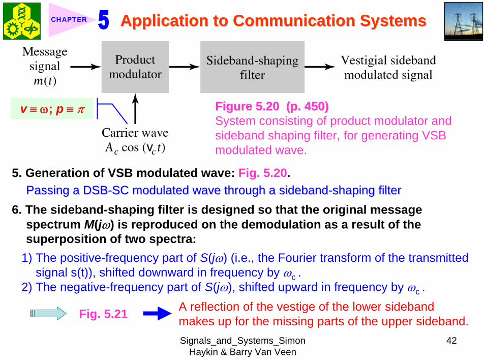
Signals_and_Systems_Simon Haykin amp Barry Van Veen
42
Application to Communication SystemsApplication to Communication SystemsCHAPTER
5 Generation of VSB modulated wave Fig 520
Figure 520 (p 450)Figure 520 (p 450)System consisting of product modulator and sideband shaping filter for generating VSB modulated wave
v equiv ω p equiv π
Passing a DSBPassing a DSB--SC modulated wave through a sidebandSC modulated wave through a sideband--shaping filtershaping filter6 The sideband-shaping filter is designed so that the original message
spectrum M(jω) is reproduced on the demodulation as a result of the superposition of two spectra
1) The positive-frequency part of S(jω) (ie the Fourier transform of the transmitted signal s(t)) shifted downward in frequency by ωc
2) The negative-frequency part of S(jω) shifted upward in frequency by ωc
Fig 521 A reflection of the vestige of the lower sideband makes up for the missing parts of the upper sideband
Signals_and_Systems_Simon Haykin amp Barry Van Veen
43
Application to Communication SystemsApplication to Communication SystemsCHAPTER
Figure 521 (p 450)Figure 521 (p 450)Superposition of the two spectra shown in parts (a) and (b) of the figure results in the original message spectrum (shown dashed) upon demodulation
58 58 PulsePulse--Amplitude Modulation Amplitude Modulation clubs Basic concept
Basic role in the operation of AM Frequency-shiftingBasic role in the operation of PAM Sampling
581 581 Sampling RevisitedSampling Revisited1 Sampling theorem
In view point of PAMIn view point of PAM
Signals_and_Systems_Simon Haykin amp Barry Van Veen
44
Application to Communication SystemsApplication to Communication SystemsCHAPTER
1) A band-limited signal of finite energy that has no radian frequency components higher than ωm is uniquely determined by the values of the signal at instants of time separated by π ωm seconds
2) A band-limited signal of finite energy that has no radian frequency components higher than ωm may be completely recovered from a knowledge of its samples taken at the rate of ωm π per seconds
clubs Part 1) rArr Be exploited in the transmitter of a PAM clubs Part 2) rArr Be exploited in the Receiver of a PAM2 To combat the effects of aliasing in practice we use two corrective measures1) Prior to sampling a low-pass antialiasing filter is used to attenuate those high-
frequency components of the signal which lie outside the band of interest2) The filtered signal is sampled at a rate slightly higher than the Nyquist rate3 Generation of a PAM signal Fig 522Fig 522Example 54 Telephonic CommunicationThe highest frequency component of a speech signal needed for telephonic communication is about 31 kHz Suggest a suitable value for the sampling rate ltltSolgtSolgt
Signals_and_Systems_Simon Haykin amp Barry Van Veen
45
Application to Communication SystemsApplication to Communication SystemsCHAPTER
Figure 522 (p 451)Figure 522 (p 451)System consisting of antialiasing filter and sample-and-hold circuit for converting a message signal into a flattopped PAM signal
1 The highest frequency component of 31 kHz corresponds to 362 10 radsmω π= times
Correspondingly the Nyquist rate is
62 kHzmωπ
=
2 A suitable value for the sampling rate-one slightly higher than the Nyquistrate-may be 8 kHz a rate that is the international standard for telephone speech signals
Signals_and_Systems_Simon Haykin amp Barry Van Veen
46
Application to Communication SystemsApplication to Communication SystemsCHAPTER
582 582 Mathematical Description of PAMMathematical Description of PAM1 The carrier wave used in PAM consists of a sequence of short pulses of
fixed duration in terms of which PAM is formally defined as followsPAM is a form of pulse modulation in which the amplitude of the PAM is a form of pulse modulation in which the amplitude of the pulsed carrier is pulsed carrier is varied in accordance with instantaneous sample values of the mesvaried in accordance with instantaneous sample values of the message signalsage signal the duration of the pulsed carrier is maintained constant throughout
Fig 523Fig 523
Figure 523 (p452) Figure 523 (p452) Waveform of flattopped PAM signal with pulse duration T0 and sampling period Ts
Signals_and_Systems_Simon Haykin amp Barry Van Veen
47
Application to Communication SystemsApplication to Communication SystemsCHAPTER
2 Mathematical representation of the PAM
( ) [ ] ( )sn
s t m n b t nTinfin
=minusinfin
= minussum (524) s(t) equiv PAM signal m(t) equiv
message signal
Ts equiv sampling period m[n] equiv the values of m(t) at t = nTs h(t) equiv rectangular pulse of the unit amplitude and duration T0
3 Rectangular pulse
01 0( )
0 otherwiset T
h tlt lt⎧
= ⎨⎩
(525) Fig 524 (a)Fig 524 (a)
clubs Eq (524) is a sample-and-hold operationAnalogous to zeroAnalogous to zero--orderorder--holdhold--
based reconstruction in Sec 46based reconstruction in Sec 46
差異差異hh((tt) ) 的的TTss與與TT00
4 Impulse-sampled version of message signal m(t)
( ) [ ] ( )sn
m t m n t nTδ δinfin
=minusinfin
= minussum (526)
5 PAM signal( ) [ ] ( )
( ) ( )
sn
s t m n b t nT
m t b tδ
infin
=minusinfin
= minus
=
sum(527)
Convolution of impulse-sampled version mδ(t) and h(t)
Time domain Time domain operationoperation
Signals_and_Systems_Simon Haykin amp Barry Van Veen
48
Application to Communication SystemsApplication to Communication SystemsCHAPTER
Figure 524 (p 453)(a) Rectangular pulse h(t) of unit amplitude and duration T0 (b) Magnitude spectrum |H(jω)| and phase spectrum argH(jω) of pulse h(t)
v equiv ω p equiv π
Signals_and_Systems_Simon Haykin amp Barry Van Veen
49
Application to Communication SystemsApplication to Communication SystemsCHAPTER
6 FT of PAM signal( ) ( ) ( )S j M j H jδω ω ω= (528)
where( ) ( )FTS j s tω larr⎯rarr ( ) ( )FTM j m tδ δω larr⎯rarr ( ) ( )FTH j h tω larr⎯rarr
7 Impulse sampling of the message signal m(t) introduces periodicity into the spectrum as given by
1( ) ( ( ))sks
M j M j kTδ ω ω ω
infin
=minusinfin
= minussum (529) 1Ts equiv sampling rate ωs = 2πTs rads
1( ) ( ( )) ( )sks
S j M j k H jT
ω ω ω ωinfin
=minusinfin
= minussum (530)
( ) ( )FTM j m tω larr⎯rarrwhere
clubs Suppose that m(t) is strictly band limited and that the sampling rate 1Ts is greater than the Nyquist rate Then passing s(t) through a reconstruction filter chosen as an ideal low-pass filter with cutoff frequency ωm and gain Ts we find that the spectrum of the resulting filter output is equal to M(jω)H(jω)
Signals_and_Systems_Simon Haykin amp Barry Van Veen
50
Application to Communication SystemsApplication to Communication SystemsCHAPTER
8 From Eq (525) we find that0 2
0 0( ) sin ( (2 )) j TH j T c T e ωω ω π minus= (531) Fig 524(b) magnitude and phase of H(jω)
clubs Using PAM to represent a continuous-time message signal we introduce amplitude distortion as well as a delay of T02
clubs The frequency distortion caused by the use of flat-topped sampled in the generation of a PAM wave illustrated in Fig 523Fig 523 is referred to as the aperture effect
583 583 Demodulation of PAM SignalDemodulation of PAM Signal1 Reconstruction scheme Fig 525Fig 525
Figure 525 (p 454)Figure 525 (p 454)System consisting of low-pass interpolation filter and equalizer for reconstructing a message signal from its flattopped sampled version
clubs The system consists of low-pass interpolation filter and equalizer connected in cascade
Signals_and_Systems_Simon Haykin amp Barry Van Veen
51
Application to Communication SystemsApplication to Communication SystemsCHAPTER
2 The cutoff frequency of low-pass filter = the highest frequency ωm of message signal
3 The equalizer is used to correct the aperture effect due to flat-topped sampling in the sample-and-hold circuit
4 The equalizer has the effect of decreasing the in-band loss of the interpolation filter as frequency increases in such a manner as to compensate for the aperture effect
5 Amplitude response of equalizer
0
0 0 0 0
1 1 1| ( ) | | sinc( 2) | 2 | sin( 2) |
TH j T T T T
ωω ω ω
= =
Frequency response Eq (531)
Example 55 Equalization for PAM TransmissionThe duty cycle in a PAM signal namely T0 Ts is 10 Evaluate the peak amplification required for equalizationltltSolgtSolgt1 At ωm = π Ts which corresponds to the highest frequency component of the
message signal for a sampling rate equal to the Nyquist rate we find from Eq (531) that the magnitude response of the equalizer at ωm normalized to that at zero frequency is
Signals_and_Systems_Simon Haykin amp Barry Van Veen
52
Application to Communication SystemsApplication to Communication SystemsCHAPTER
Figure 526 (p 455)Figure 526 (p 455)Normalized equalization (to compensate for aperture effect) plotted against the duty cycle T0Ts
Signals_and_Systems_Simon Haykin amp Barry Van Veen
53
Application to Communication SystemsApplication to Communication SystemsCHAPTER
0
0 0
( 2)( )1sin (05 ) sin[( 2)( )]
s
s s
T Tc T T T T
ππ
=
where the ratio T0 Ts is equal to the duty cycle of the sampling pulses 2 In Fig 526Fig 526 this result is plotted as a function of the duty cycle T0 Ts Ideally it
should be equal to unity for all values of T0 Ts 3 For a duty cycle of 10 it is equal to 10041 It follows that for duty cycles of less
than 10 the magnitude equalization required is less than 10041 in which case the aperture effect is usually considered to be negligible
59 59 Multiplexing Multiplexing clubs Three basic types of multiplexing1 Frequency-division multiplexing in which the signals are separated by
allocating them to different frequency bands This is illustrated in Fig 527(a) for the case of six different message signals Frequency-division multiplexing favors the use of CW modulation where each message signal is able to use the channel on a continuous-time basis
2 Time-division multiplexing wherein the signals are separated by allocating them to different time slots within a sampling interval
Signals_and_Systems_Simon Haykin amp Barry Van Veen
54
Application to Communication SystemsApplication to Communication SystemsCHAPTER
This second type of multiplexing is illustrated in Fig 527(b) for the case of six different message signals Code-division multiplexing which relies on the assignment of different codes to the individual users of the channel
3 Code-division multiplexing which relies on the assignment of different codes to the individual users of the channel
591 591 FrequencyFrequency--Domain Multiplexing (FDM)Domain Multiplexing (FDM)1 Block diagram Fig 528Fig 5282 Incoming message signals low-pass variety3 Low-pass filter to remove high-frequency components such that the signal
in each channel does not disturb each other4 MOD (modulator) shift the frequency ranges of the signals so as to occupy
mutually exclusive frequency intervalsSSB is often used in this stageEx Voice input is usually assigned a bandwidth of 4 kHz
5 Band-pass filters are used to restrict the band of each modulated wave to its prescribed range
6 Band-pass filters in receiver separate the message signals7 DEM (demodulator) to recover signalsclubs FDM in Fig 528 operates in only one direction
Signals_and_Systems_Simon Haykin amp Barry Van Veen
55
Application to Communication SystemsApplication to Communication SystemsCHAPTER
Figure 527 (p 456)Figure 527 (p 456)Two basic forms of multiplexing (a) Frequency-division multiplexing (with guardbands) (b) Time-division multiplexing no provision is made here for synchronizing pulses
Signals_and_Systems_Simon Haykin amp Barry Van Veen
56
Application to Communication SystemsApplication to Communication SystemsCHAPTER
Figure 528 (p 457)Figure 528 (p 457)Block diagram of FDM system showing the important constituents of the transmitter and receiver
Signals_and_Systems_Simon Haykin amp Barry Van Veen
57
Application to Communication SystemsApplication to Communication SystemsCHAPTER
Example 56 SSB-FDM System
ltltSolgtSolgt
An FDM system is used to multiplex 24 independent voice signals SSB modulation is used for the transmission Given that each voice signal is allotted a bandwidth 4kHz calculate the overall transmission bandwidth of the channel
With each voice signal allotted a bandwidth of 4 kHz the use of SSB modulation requires a bandwidth of 4 kHz for its transmission Accordingly the overall transmission bandwidth provided by the channel is 24 X 4 = 96 kHz 592 592 TimeTime--Domain Multiplexing (TDM)Domain Multiplexing (TDM)clubs Basic to the operation of a TDM system is the sampling theoremclubs The transmission of the message samples engages the transmission channel for
only a fraction of the sampling interval on a periodic basis equal to the width T0 of a PAM modulating pulse
1 Block diagram Fig 529Fig 5292 Commutator is usually implemented by means of electronic switching
circuitry3 The function of commutator is two folds
Signals_and_Systems_Simon Haykin amp Barry Van Veen
58
Application to Communication SystemsApplication to Communication SystemsCHAPTER
Figure 529 (p 458)Figure 529 (p 458)Block diagram of TDM system showing the important constituents of the transmitter and receiver
(1) To take a narrow sample of each of the M input message signals at a rate 1Tsthat is slightly higher than ωcπ where ωc is the cutoff frequency of the input low-pass filter
(2) To sequentially interleave these M samples inside a sampling interval Ts4 Pulse modulator transform the multiplexed signal into a form suitable for
transmission over the common channel
Signals_and_Systems_Simon Haykin amp Barry Van Veen
59
Application to Communication SystemsApplication to Communication SystemsCHAPTER
clubs The use of time-division multiplexing introduces a bandwidth expansion factor M because the scheme must squeeze M samples derived from M independent message sources into a time slot equal to one sampling interval
5 Pulse demodulator performs the inverse operation of the pulse modulator6 Decommutator distributes the narrow samples produced by pulse demodulator to the appropriate low-pass reconstruction filter7 Synchronization between the timing operations of the transmitter and
receiver in a TDM system is essential for satisfactory performance of the system
Inserting an extra pulse into each sampling interval on a regular basisBandwidth expansion factor is increased to M + 1
clubs The TDM system is hghly sensitive to the dispersion in the common transmission channel
Example 57 Comparison of TDM with FDMATDM system is used to multiplex four independent voice signals using PAM Each voice signal is sampled at the rate of 8 kHz The system incorporates a synchronizing pulse train for its proper operation
Signals_and_Systems_Simon Haykin amp Barry Van Veen
60
Application to Communication SystemsApplication to Communication SystemsCHAPTER
(a) Determine the timing relationships between the synchronizing pulse train and the impulse trains used to sample the four voice signals
(b) Calculate the transmission bandwidth of the channel for the TDM system and compare the result with a corresponding FDM system using SSBmodulation
ltltSolgtSolgt(a) The sampling period is
31 125 s
8 10sT s μ= =times
In this example the number of voice signals is M = 4 Hence dividing the sampling period of 125 μs among these voice signals and the synchronizing pulse train we obtain the time slot allocated to each one of them
0 1125 25 s
5
sTTM
μ
=+
= =
Signals_and_Systems_Simon Haykin amp Barry Van Veen
61
Application to Communication SystemsApplication to Communication SystemsCHAPTER
Figure 530Figure 530 shows the timing relationships between the synchronizing pulse train and the four impulse trains used to sample the different voice signals in a single frame Each frame includes time slots of common duration T0 = 25 μs which are allocated to the pulse-modulated signals and synchronizing pulse
Figure 530 (p 459)Figure 530 (p 459)Composition of one frame of a multiplexed PAM signal incorporating four voice-signals and a synchronizing pulse
Signals_and_Systems_Simon Haykin amp Barry Van Veen
62
Application to Communication SystemsApplication to Communication SystemsCHAPTER
(b) As a consequence of the time-bandwidth product (see Section 317) there is an inverse relationship between the duration of a pulse and the bandwidth (ie cutoff frequency) of the channel needed for itstransmission Accordingly the overall transmission bandwidth of the channel is
0
21 1 MHz 40 kHz
25
TTf
T
ωπ
=
= = =
In contrast the use of an FDM system based on SSB modulation requires a channel bandwidth equal to M times that of a single voice signal-that is 4 X 4 = 16 kHz Thus the use of PAM-TDM requires a channel bandwidth that is 40 16 = 25 times that of SSB-FDMIn practice pulse-code modulation is commonly used as the method of modulation for TDM this results in a further increase in channel bandwidth depending on the length of the code word used in the digital representation of each pulse in the PAM signal
Signals_and_Systems_Simon Haykin amp Barry Van Veen
63
Application to Communication SystemsApplication to Communication SystemsCHAPTER
510 510 Pulse and Group Delays Pulse and Group Delays 1 Whenever a signal is transmitted through a dispersive (ie frequency
selective) system some delay is introduced into the output signal in relation to the input signal
2 The delay is determined by the phase response of the system3 Phase response of a dispersive communication channel
( ) arg ( )H jφ ω ω= (532)
A signal is transmitted through the channel at a frequency ωc The signal received at the channel lags the transmitted signal by φ(ωc) The time delay is called phase delay formally defined as
( )cp
c
φ ωτω
= minus (533)
The phase delay is not necessarily the true signal delayclubs Case study for DSB-SC1 Transmitted signal
0( ) cos( ) cos( )cs t A t tω ω= (534)
ωc equiv carrier frequency ω0 equiv sinusoidal modulation frequency
A = AcA0
Signals_and_Systems_Simon Haykin amp Barry Van Veen
64
Application to Communication SystemsApplication to Communication SystemsCHAPTER
1 21 1( ) cos( ) cos( )2 2
s t A t A tω ω= +
1 0cω ω ω= + (535) where
2 0cω ω ω= minus (536)
Upper frequency
Lower frequency
2 Let the s(t) be transmitted through the channel with phase response φ (ω) Accordingly the signal received at the channel output is
1 1 2 21 1( ) cos( ( )) cos( ( ))2 2
y t A t A tω φ ω ω φ ω= + + +
1 2 1 20
( ) ( ) ( )1 ( )( ) cos cos2 2cy t A t tφ ω φ ω φ ω φ ωω ω+⎛ ⎞ ⎛ ⎞= + +⎜ ⎟ ⎜ ⎟
⎝ ⎠ ⎝ ⎠(537)
3 Two observations from Eq (537)1) The carrier component at frequency ωc in y(t) lags its counterpart in s(t) by
frac12 (φ (ω1) + φ (ω2)) which represents a time delay equal to
1 2 1 2
c 1 2
( )+ ( ) ( )+ ( )2 +
φ ω φ ω φ ω φ ωω ω ω
minus = minus (538)
Signals_and_Systems_Simon Haykin amp Barry Van Veen
65
Application to Communication SystemsApplication to Communication SystemsCHAPTER
2) The message component at frequency ω0 in y(t) lags its counterpart in s(t) by frac12 (φ (ω1) minus φ (ω2)) which represents a time delay equal to
1 2 1 2
0 1 2
( ) ( ) ( ) ( )2
φ ω φ ω φ ω φ ωω ω ωminus minus
minus = minusminus
(539)
4 Suppose that ω0 lt ωc rArr the side frequencies are close together with ω c between them Such a modulated signal is said to be a narrowband signal The phase response φ (ω) in the vicinity of ω = ωc is approximated by two-term Taylor series expansion
( )( ) ( ) ( )c
c cd
d ω ω
φ ωφ ω φ ω ω ωω =
= + times minus (540)
Phase delay = ( ) c cφ ω ωminus
5 The time delay introduced by the message signal (ie he ldquoenveloperdquo of the modulated signal) is given by
( )
c
gd
d ω ω
φ ωτω =
= minus (541) The time delay τg is called the
envelope delay or group delay
Signals_and_Systems_Simon Haykin amp Barry Van Veen
66
Application to Communication SystemsApplication to Communication SystemsCHAPTER
6 When a modulated signal is transmitted through a communication channel there are two different delays to be considered1) The carrier or phase delay τp defined by Eq (533)2) The envelope or group delay τg defined by Eq (541)
clubs The group delay is the true signal delay
Example 58 Phase and Group Delays for Ban-pass Channel
ltltSolgtSolgt
The phase response of a band-pass communication channel is defined by 2 2
1( ) tan c
c
ω ωφ ωωω
minus ⎛ ⎞minus= minus ⎜ ⎟
⎝ ⎠The signal s(t) defined in Eq (534) is transmitted through this channel with
475 radscω = 0 025 radsω =andCalculate (a) the phase delay and (b) the group delay
(a) At ω = ωc φ (ωc) = 0 According to Eq (533) the phase delay τ p is zero (b) Differentiating φ (ω) with respect to ω we get
Signals_and_Systems_Simon Haykin amp Barry Van Veen
67
Application to Communication SystemsApplication to Communication SystemsCHAPTER
2 2
2 2 2 2 2
( )( )( )
c c
c c
dd
ω ω ωφ ωω ω ω ω ω
+= minus
+ minus
Using thing result in Eq (541) we find that the group delay is 2 2 04211
475gc
sτω
= = =
1 One waveform shown as a solid curve was obtained by multiplying the transmitted signal s(t) by the carrier wave cos(ωct)
2 The second waveform shown as a dotted curve was obtained by multiplying the received signal y(t) by the carrier wave cos(ωct)
To display the results obtained in parts (a) and (b) in graphical form Fig 531Fig 531shows a superposition of two waveforms obtained as follows
The figure clearly shows that the carrier (phase) delay τ p is zero and the envelope of the received signal y(t) is lagging behind that of the transmitted signal by τs seconds For the presentation of waveforms in this figure we purposely did not use a filter to suppress the high frequency components resulting from the multiplications described under points 1 and 2 because of the desire to retain a contribution due to the carrier for display
Signals_and_Systems_Simon Haykin amp Barry Van Veen
68
Application to Communication SystemsApplication to Communication SystemsCHAPTER
Figure 531 Figure 531 (p 463)(p 463)Highlighting the zero carrier delay (solid curve) and group delay τg (dotted curve) which are determined in accordance with Example 58
Signals_and_Systems_Simon Haykin amp Barry Van Veen
69
Application to Communication SystemsApplication to Communication SystemsCHAPTER
clubs Not also that the separation between the upper side frequency ω1 = ωc + ω0 = 500 rads and the lower side frequency ω2 = ωc minus ω0 = 450 rads is about 10 of the carrier frequency ωc = 475 rads which justifies referring to the modulated signal in this example as a narrowband signal
5101 5101 Some Practical ConsiderationsSome Practical Considerationsclubs What is the practical importance of group delay 1 Eq (541) for determining group delay applies strictly to narrowband
modulated signal2 The message bandwidth may be comparable to the carrier frequency In
this situation the group delay is formulated as a frequency-dependent parameter ie ( )d( )g d
φ ωτ ωω
= minus (542)
3 When a wideband modulated signals transmitted through a dispersive channel the frequency components of the message signal are delayed by different amounts at the channel output
Delay distortionFig 532Fig 532 Group delay response of voice-grade telephone channel
Signals_and_Systems_Simon Haykin amp Barry Van Veen
70
Application to Communication SystemsApplication to Communication SystemsCHAPTER
Figure 532 (p 464)Group delay response of voice-grade telephone channel (Adapted from J C Bellamy Digital Telephony Wiley 1982)
511 511 Exploring Concepts with MATLABExploring Concepts with MATLAB5111 5111 Full AMFull AMclubs Sinusoidal modulation
clubs To reconstruct a faithful version of the original message signal in the receiver we have to use a delay equalizer
0( ) [1 cos( )]cos( )c cs t A t tμ ω ω= +1 AM experiment
1cA =
08 radscω π= 0 01 radsω π=Carrier amplitude
Carrier frequency Modulation amplitude
Signals_and_Systems_Simon Haykin amp Barry Van Veen
71
Application to Communication SystemsApplication to Communication SystemsCHAPTER
2 We wish to display and analyze 10 full cycles of the AM wave corresponding to a total duration of 200 s Choosing a sampling rate 1Ts = 10 Hz we have a total of N = 2000 time samples The frequency band of interest is minus 10 π ≦ ω ≦ 10 π Since the separation between the carrier and either side frequency is equal to the modulation frequency ω0 = 01 π rads we would like to have a frequency resolution ωr = 001π rads To achieve this resolution we require the following number of frequency samples (see Eq (442))
20 2000001
s
r
M ω πω π
ge = =
3 We therefore choose M = 2000 To approximate the Fourier transform of the AM wave s(t) we may use a 2000-point DTFS The only variable in the AM experiment is the modulation factor μ with respect to which we wish to investigate three different situationsμ = 05 corresponding to under-modulationμ = 10 for which the AM system is on the verge of over-modulationμ = 20 corresponding to over-modulation
Signals_and_Systems_Simon Haykin amp Barry Van Veen
72
Application to Communication SystemsApplication to Communication SystemsCHAPTER
4 MATLAB commandsAc = 1 carrier amplitudewc = 08pi carrier frequencyw0 = 01pi modulation frequencymu = 05 modulation factort = 0011999s = Ac(1 + mucos(w0t))cos(wct)plot(ts)Smag = abs(fftshift(fft(s2000)))2000 Smag denotes the magnitude specturm of the AM wavew = 10[-1000999]2pi2000plot(wSmag)axis ([-30 30 0 08])
5 5 μμ = 05 = 05 case case Fig 533Fig 533μμ = 10 case = 10 case Fig 534Fig 534μμ = 20 case = 20 case Fig 535Fig 535
Discussion see pp 466-469 textbook
Signals_and_Systems_Simon Haykin amp Barry Van Veen
73
Application to Communication SystemsApplication to Communication SystemsCHAPTER
-30 -20 -10 0 10 20 300
02
04
06
0 50 100 150 200-2
-1
0
1
2
2 22 24 26 28 3
02
04
06
(a) Time (s)
Time domain
Frequency domain
(b) Frequency (rads)
Frequency domain
Frequency (rads)
Figure 533 (p 466)Amplitude modulation with 50 modulation (a) AM wave (b) magnitude spectrum of the AM wave and (c) expanded spectrum around the carrier frequency
μμ = 05 = 05 casecase
Signals_and_Systems_Simon Haykin amp Barry Van Veen
74
Application to Communication SystemsApplication to Communication SystemsCHAPTER
Figure 534 (p 467)Figure 534 (p 467)Amplitude modulation with 100 modulation (a) AM wave (b) magnitude spectrum of the AM wave and (c) expanded spectrum around the carrier frequency
Signals_and_Systems_Simon Haykin amp Barry Van Veen
75
Application to Communication SystemsApplication to Communication SystemsCHAPTER
Figure 535 (p 468)Amplitude modulation with 200 modulation (a) AM wave (b) magnitude spectrum of the AM wave and (c) expanded spectrum around the carrier frequency
Signals_and_Systems_Simon Haykin amp Barry Van Veen
76
Application to Communication SystemsApplication to Communication SystemsCHAPTER
5112 5112 DSBDSB--SC ModulationSC Modulation1 Sinusoidal modulation
0 0( ) cos( ) cos( )c cs t A A t tω ω=
2 MATLAB commands
Ac = 1 carrier amplitudewc = 08pi carrier frequency in radsA0 = 1 amplitude of modulating signalw0 = 01pi frequency of modulating signalt = 011999s = AcA0cos(wct)cos(w0t)plot(ts)Smag = abs(fftshift(fft(s2000)))2000w = 10[-1000999]2pi2000plot(wSmag)
3 3 DSBDSB--SC modulated waveSC modulated wave Fig 536Fig 536 Discussion see pp 466-469 textbook
4 Output of the product modulator in Fig 512 (b) with φ = 0
Signals_and_Systems_Simon Haykin amp Barry Van Veen
77
Application to Communication SystemsApplication to Communication SystemsCHAPTER
Figure 536 (p 469)DSB-SC modulation (a) DSB-SC modulated wave (b) magnitude spectrum of the modulated wave and (c) expanded spectrum around the carrier frequency
Signals_and_Systems_Simon Haykin amp Barry Van Veen
78
Application to Communication SystemsApplication to Communication SystemsCHAPTER
( ) ( ) cos( )cv t s t tω=
5 MATLAB commandsgtgt v = scos(wct)
6 Fig 537 (a) waveforms of v(t) Fig 537 (b) magnitude spectrum which readily shows that v(t) consists of the following components1) A sinusoidal component with frequency 01π rads representing the
modulating wave2) A new DSB-SC modulated wave with double carrier frequency of 16π rads
in actuality the side frequencies of this modulated wave are located at 15πand 17π rads
1) The frequency of the modulating wave lies inside the passband of the filter2) The upper and lower side frequencies of the new DSB-SC modulated wave
lie inside the stopband of the filter
Accordingly we may recover the sinusoidal modulating signal by passing v(t) through low-pass filter with the following requirements
Signals_and_Systems_Simon Haykin amp Barry Van Veen
79
Application to Communication SystemsApplication to Communication SystemsCHAPTER
Figure 537 (p 470)Coherent detection of DSB-SC modulated wave (a) and (b) Waveform and magnitude spectrum of signal produced at the output of produce modulator (c) and (d) waveform and magnitude spectrum of low-pass filter output
Signals_and_Systems_Simon Haykin amp Barry Van Veen
80
Application to Communication SystemsApplication to Communication SystemsCHAPTER
The issue of how to design a filter with these requirements will be considered in detail in Chapter 8 For the present it suffices to say that the preceding requirements can be met by using the following MATLAB commands
gtgt [ba] = butter(30025)gtgt output = filter(bav)
The first command produces s special type of filter called a Butterworth filter For the experiment considered here the filter order is 3 and its normalized cutoff frequency of 0025 is calculated as follows
Actual cutoff frequency of filter 025 radsHalf the sampling rate 10 rads
0025
ππ
=
=
The second command computes the filterrsquos output in response to the product modulator output v(t) (We will revisit the design of this filter in Chapter 8) Figure 537(c) displays the waveform of the low-pass filter output this waveform represents a sinusoidal signal of frequency 005 Hz an observation that is confirmed by using the ffr command to approximate the spectrum of the filter output The result of the computation is shown in Fig 537(d)Fig 537(d)
Signals_and_Systems_Simon Haykin amp Barry Van Veen
81
Application to Communication SystemsApplication to Communication SystemsCHAPTER
7 In Fig 538 we explore another aspect of DSB-SC modulation namely the effect of varying the modulation frequency Figure 538(a) shows five cycles of a DSB-SC modulated wave that has the same carrier frequency as that in Fig 536(a) but the modulation frequency has been reduced to 0025 Hz( ie a radian frequency of 005π) Figure 538(b) shows the magnitude spectrum of this second DSB-SC modulated wave and its zoomed-in version is shown in Fig 538(c) Comparing this latter figure with Fig 536(c) we see clearly that decreasing the modulation frequency has the effect of moving the upper and lower side frequencies closer together which is consistent with modulation theory
5113 5113 Phase and Group DelayPhase and Group Delay1 In Example 58 we studied the phase and group delays for a band-pass
channel with phase response 2 2
1( ) tan c
c
ω ωφ ωωω
minus ⎛ ⎞minus= minus ⎜ ⎟
⎝ ⎠2 At ω = ωc the phase delay is τ p = 0 and the group delay is τ s = 04211s One
of the wave forms displayed in Fig 531Fig 531 is
1( ) ( ) cos( )cx t s t tω=
Signals_and_Systems_Simon Haykin amp Barry Van Veen
82
Application to Communication SystemsApplication to Communication SystemsCHAPTER
Figure 538 (p 472)Effect of varying the modulation frequency compared with that in Fig 537 (a) and (b) Waveform and magnitude spectrum of DSB-SC modulated wave with a modulation frequency one-half that used in Fig 536 (c) expanded spectrum around the carrier frequency
Signals_and_Systems_Simon Haykin amp Barry Van Veen
83
Application to Communication SystemsApplication to Communication SystemsCHAPTER
where (see page 461)
1 2( ) [cos( ) cos( )]2As t t tω ω= +
and ω1 = ωc + ω0 and ω2 = ωc - ω0 The waveform shown in the figure as a solid curve is a plot of x1(t) The other waveform also displayed in Fig 531Fig 531 is
2
1 1 2 2
( ) ( ) cos( )
[cos( ( )) cos( ( ))]cos( )2
c
c
x t y t tA t t t
ω
ω φ ω ω φ ω ω
=
= + + +
where the angle φ (ω1) and φ (ω2) are the values of the phase response φ (ω) at ω = ω1 and ω = ω2 respectively The waveform shown as a dotted curve in the figure is a plot of x2(t)
3 The generation of x1(t) and x2(t) in MATLAB is achieved with the following commands with A2 set equal to unity
Signals_and_Systems_Simon Haykin amp Barry Van Veen
84
Application to Communication SystemsApplication to Communication SystemsCHAPTER
wc = 475w0 = 025w1 = wc + w0w2 = wc - w0t = -10 0001 10o1 = -atan((w1^2 - wc^2)(w1wc))o2 = -atan((w2^2 - wc^2)(w2wc))s = cos(w1t) + cos(w2t)y = cos(w1t + o1) + cos(w2t + o2)x1 = scos(478t)x2 = ycos(475t)plot(tx1b)hold on plot(tx2k)hold offxlabel(Time)ylabel(Amplitude)
Note that we have set (A2) = 1 for convenience of presentation The function atan in the first two commands returns the arctangent Note also that the computation of both x1 and x2 involve element-by-element multiplications ndash hence the use of period followed by an asterisk
Signals_and_Systems_Simon Haykin amp Barry Van Veen
85
Application to Communication SystemsApplication to Communication SystemsCHAPTER
Signals_and_Systems_Simon Haykin amp Barry Van Veen
86
Application to Communication SystemsApplication to Communication SystemsCHAPTER
Signals_and_Systems_Simon Haykin amp Barry Van Veen
87
Application to Communication SystemsApplication to Communication SystemsCHAPTER
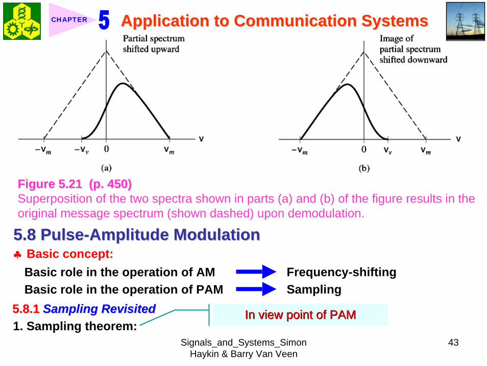
Signals_and_Systems_Simon Haykin amp Barry Van Veen
43
Application to Communication SystemsApplication to Communication SystemsCHAPTER
Figure 521 (p 450)Figure 521 (p 450)Superposition of the two spectra shown in parts (a) and (b) of the figure results in the original message spectrum (shown dashed) upon demodulation
58 58 PulsePulse--Amplitude Modulation Amplitude Modulation clubs Basic concept
Basic role in the operation of AM Frequency-shiftingBasic role in the operation of PAM Sampling
581 581 Sampling RevisitedSampling Revisited1 Sampling theorem
In view point of PAMIn view point of PAM
Signals_and_Systems_Simon Haykin amp Barry Van Veen
44
Application to Communication SystemsApplication to Communication SystemsCHAPTER
1) A band-limited signal of finite energy that has no radian frequency components higher than ωm is uniquely determined by the values of the signal at instants of time separated by π ωm seconds
2) A band-limited signal of finite energy that has no radian frequency components higher than ωm may be completely recovered from a knowledge of its samples taken at the rate of ωm π per seconds
clubs Part 1) rArr Be exploited in the transmitter of a PAM clubs Part 2) rArr Be exploited in the Receiver of a PAM2 To combat the effects of aliasing in practice we use two corrective measures1) Prior to sampling a low-pass antialiasing filter is used to attenuate those high-
frequency components of the signal which lie outside the band of interest2) The filtered signal is sampled at a rate slightly higher than the Nyquist rate3 Generation of a PAM signal Fig 522Fig 522Example 54 Telephonic CommunicationThe highest frequency component of a speech signal needed for telephonic communication is about 31 kHz Suggest a suitable value for the sampling rate ltltSolgtSolgt
Signals_and_Systems_Simon Haykin amp Barry Van Veen
45
Application to Communication SystemsApplication to Communication SystemsCHAPTER
Figure 522 (p 451)Figure 522 (p 451)System consisting of antialiasing filter and sample-and-hold circuit for converting a message signal into a flattopped PAM signal
1 The highest frequency component of 31 kHz corresponds to 362 10 radsmω π= times
Correspondingly the Nyquist rate is
62 kHzmωπ
=
2 A suitable value for the sampling rate-one slightly higher than the Nyquistrate-may be 8 kHz a rate that is the international standard for telephone speech signals
Signals_and_Systems_Simon Haykin amp Barry Van Veen
46
Application to Communication SystemsApplication to Communication SystemsCHAPTER
582 582 Mathematical Description of PAMMathematical Description of PAM1 The carrier wave used in PAM consists of a sequence of short pulses of
fixed duration in terms of which PAM is formally defined as followsPAM is a form of pulse modulation in which the amplitude of the PAM is a form of pulse modulation in which the amplitude of the pulsed carrier is pulsed carrier is varied in accordance with instantaneous sample values of the mesvaried in accordance with instantaneous sample values of the message signalsage signal the duration of the pulsed carrier is maintained constant throughout
Fig 523Fig 523
Figure 523 (p452) Figure 523 (p452) Waveform of flattopped PAM signal with pulse duration T0 and sampling period Ts
Signals_and_Systems_Simon Haykin amp Barry Van Veen
47
Application to Communication SystemsApplication to Communication SystemsCHAPTER
2 Mathematical representation of the PAM
( ) [ ] ( )sn
s t m n b t nTinfin
=minusinfin
= minussum (524) s(t) equiv PAM signal m(t) equiv
message signal
Ts equiv sampling period m[n] equiv the values of m(t) at t = nTs h(t) equiv rectangular pulse of the unit amplitude and duration T0
3 Rectangular pulse
01 0( )
0 otherwiset T
h tlt lt⎧
= ⎨⎩
(525) Fig 524 (a)Fig 524 (a)
clubs Eq (524) is a sample-and-hold operationAnalogous to zeroAnalogous to zero--orderorder--holdhold--
based reconstruction in Sec 46based reconstruction in Sec 46
差異差異hh((tt) ) 的的TTss與與TT00
4 Impulse-sampled version of message signal m(t)
( ) [ ] ( )sn
m t m n t nTδ δinfin
=minusinfin
= minussum (526)
5 PAM signal( ) [ ] ( )
( ) ( )
sn
s t m n b t nT
m t b tδ
infin
=minusinfin
= minus
=
sum(527)
Convolution of impulse-sampled version mδ(t) and h(t)
Time domain Time domain operationoperation
Signals_and_Systems_Simon Haykin amp Barry Van Veen
48
Application to Communication SystemsApplication to Communication SystemsCHAPTER
Figure 524 (p 453)(a) Rectangular pulse h(t) of unit amplitude and duration T0 (b) Magnitude spectrum |H(jω)| and phase spectrum argH(jω) of pulse h(t)
v equiv ω p equiv π
Signals_and_Systems_Simon Haykin amp Barry Van Veen
49
Application to Communication SystemsApplication to Communication SystemsCHAPTER
6 FT of PAM signal( ) ( ) ( )S j M j H jδω ω ω= (528)
where( ) ( )FTS j s tω larr⎯rarr ( ) ( )FTM j m tδ δω larr⎯rarr ( ) ( )FTH j h tω larr⎯rarr
7 Impulse sampling of the message signal m(t) introduces periodicity into the spectrum as given by
1( ) ( ( ))sks
M j M j kTδ ω ω ω
infin
=minusinfin
= minussum (529) 1Ts equiv sampling rate ωs = 2πTs rads
1( ) ( ( )) ( )sks
S j M j k H jT
ω ω ω ωinfin
=minusinfin
= minussum (530)
( ) ( )FTM j m tω larr⎯rarrwhere
clubs Suppose that m(t) is strictly band limited and that the sampling rate 1Ts is greater than the Nyquist rate Then passing s(t) through a reconstruction filter chosen as an ideal low-pass filter with cutoff frequency ωm and gain Ts we find that the spectrum of the resulting filter output is equal to M(jω)H(jω)
Signals_and_Systems_Simon Haykin amp Barry Van Veen
50
Application to Communication SystemsApplication to Communication SystemsCHAPTER
8 From Eq (525) we find that0 2
0 0( ) sin ( (2 )) j TH j T c T e ωω ω π minus= (531) Fig 524(b) magnitude and phase of H(jω)
clubs Using PAM to represent a continuous-time message signal we introduce amplitude distortion as well as a delay of T02
clubs The frequency distortion caused by the use of flat-topped sampled in the generation of a PAM wave illustrated in Fig 523Fig 523 is referred to as the aperture effect
583 583 Demodulation of PAM SignalDemodulation of PAM Signal1 Reconstruction scheme Fig 525Fig 525
Figure 525 (p 454)Figure 525 (p 454)System consisting of low-pass interpolation filter and equalizer for reconstructing a message signal from its flattopped sampled version
clubs The system consists of low-pass interpolation filter and equalizer connected in cascade
Signals_and_Systems_Simon Haykin amp Barry Van Veen
51
Application to Communication SystemsApplication to Communication SystemsCHAPTER
2 The cutoff frequency of low-pass filter = the highest frequency ωm of message signal
3 The equalizer is used to correct the aperture effect due to flat-topped sampling in the sample-and-hold circuit
4 The equalizer has the effect of decreasing the in-band loss of the interpolation filter as frequency increases in such a manner as to compensate for the aperture effect
5 Amplitude response of equalizer
0
0 0 0 0
1 1 1| ( ) | | sinc( 2) | 2 | sin( 2) |
TH j T T T T
ωω ω ω
= =
Frequency response Eq (531)
Example 55 Equalization for PAM TransmissionThe duty cycle in a PAM signal namely T0 Ts is 10 Evaluate the peak amplification required for equalizationltltSolgtSolgt1 At ωm = π Ts which corresponds to the highest frequency component of the
message signal for a sampling rate equal to the Nyquist rate we find from Eq (531) that the magnitude response of the equalizer at ωm normalized to that at zero frequency is
Signals_and_Systems_Simon Haykin amp Barry Van Veen
52
Application to Communication SystemsApplication to Communication SystemsCHAPTER
Figure 526 (p 455)Figure 526 (p 455)Normalized equalization (to compensate for aperture effect) plotted against the duty cycle T0Ts
Signals_and_Systems_Simon Haykin amp Barry Van Veen
53
Application to Communication SystemsApplication to Communication SystemsCHAPTER
0
0 0
( 2)( )1sin (05 ) sin[( 2)( )]
s
s s
T Tc T T T T
ππ
=
where the ratio T0 Ts is equal to the duty cycle of the sampling pulses 2 In Fig 526Fig 526 this result is plotted as a function of the duty cycle T0 Ts Ideally it
should be equal to unity for all values of T0 Ts 3 For a duty cycle of 10 it is equal to 10041 It follows that for duty cycles of less
than 10 the magnitude equalization required is less than 10041 in which case the aperture effect is usually considered to be negligible
59 59 Multiplexing Multiplexing clubs Three basic types of multiplexing1 Frequency-division multiplexing in which the signals are separated by
allocating them to different frequency bands This is illustrated in Fig 527(a) for the case of six different message signals Frequency-division multiplexing favors the use of CW modulation where each message signal is able to use the channel on a continuous-time basis
2 Time-division multiplexing wherein the signals are separated by allocating them to different time slots within a sampling interval
Signals_and_Systems_Simon Haykin amp Barry Van Veen
54
Application to Communication SystemsApplication to Communication SystemsCHAPTER
This second type of multiplexing is illustrated in Fig 527(b) for the case of six different message signals Code-division multiplexing which relies on the assignment of different codes to the individual users of the channel
3 Code-division multiplexing which relies on the assignment of different codes to the individual users of the channel
591 591 FrequencyFrequency--Domain Multiplexing (FDM)Domain Multiplexing (FDM)1 Block diagram Fig 528Fig 5282 Incoming message signals low-pass variety3 Low-pass filter to remove high-frequency components such that the signal
in each channel does not disturb each other4 MOD (modulator) shift the frequency ranges of the signals so as to occupy
mutually exclusive frequency intervalsSSB is often used in this stageEx Voice input is usually assigned a bandwidth of 4 kHz
5 Band-pass filters are used to restrict the band of each modulated wave to its prescribed range
6 Band-pass filters in receiver separate the message signals7 DEM (demodulator) to recover signalsclubs FDM in Fig 528 operates in only one direction
Signals_and_Systems_Simon Haykin amp Barry Van Veen
55
Application to Communication SystemsApplication to Communication SystemsCHAPTER
Figure 527 (p 456)Figure 527 (p 456)Two basic forms of multiplexing (a) Frequency-division multiplexing (with guardbands) (b) Time-division multiplexing no provision is made here for synchronizing pulses
Signals_and_Systems_Simon Haykin amp Barry Van Veen
56
Application to Communication SystemsApplication to Communication SystemsCHAPTER
Figure 528 (p 457)Figure 528 (p 457)Block diagram of FDM system showing the important constituents of the transmitter and receiver
Signals_and_Systems_Simon Haykin amp Barry Van Veen
57
Application to Communication SystemsApplication to Communication SystemsCHAPTER
Example 56 SSB-FDM System
ltltSolgtSolgt
An FDM system is used to multiplex 24 independent voice signals SSB modulation is used for the transmission Given that each voice signal is allotted a bandwidth 4kHz calculate the overall transmission bandwidth of the channel
With each voice signal allotted a bandwidth of 4 kHz the use of SSB modulation requires a bandwidth of 4 kHz for its transmission Accordingly the overall transmission bandwidth provided by the channel is 24 X 4 = 96 kHz 592 592 TimeTime--Domain Multiplexing (TDM)Domain Multiplexing (TDM)clubs Basic to the operation of a TDM system is the sampling theoremclubs The transmission of the message samples engages the transmission channel for
only a fraction of the sampling interval on a periodic basis equal to the width T0 of a PAM modulating pulse
1 Block diagram Fig 529Fig 5292 Commutator is usually implemented by means of electronic switching
circuitry3 The function of commutator is two folds
Signals_and_Systems_Simon Haykin amp Barry Van Veen
58
Application to Communication SystemsApplication to Communication SystemsCHAPTER
Figure 529 (p 458)Figure 529 (p 458)Block diagram of TDM system showing the important constituents of the transmitter and receiver
(1) To take a narrow sample of each of the M input message signals at a rate 1Tsthat is slightly higher than ωcπ where ωc is the cutoff frequency of the input low-pass filter
(2) To sequentially interleave these M samples inside a sampling interval Ts4 Pulse modulator transform the multiplexed signal into a form suitable for
transmission over the common channel
Signals_and_Systems_Simon Haykin amp Barry Van Veen
59
Application to Communication SystemsApplication to Communication SystemsCHAPTER
clubs The use of time-division multiplexing introduces a bandwidth expansion factor M because the scheme must squeeze M samples derived from M independent message sources into a time slot equal to one sampling interval
5 Pulse demodulator performs the inverse operation of the pulse modulator6 Decommutator distributes the narrow samples produced by pulse demodulator to the appropriate low-pass reconstruction filter7 Synchronization between the timing operations of the transmitter and
receiver in a TDM system is essential for satisfactory performance of the system
Inserting an extra pulse into each sampling interval on a regular basisBandwidth expansion factor is increased to M + 1
clubs The TDM system is hghly sensitive to the dispersion in the common transmission channel
Example 57 Comparison of TDM with FDMATDM system is used to multiplex four independent voice signals using PAM Each voice signal is sampled at the rate of 8 kHz The system incorporates a synchronizing pulse train for its proper operation
Signals_and_Systems_Simon Haykin amp Barry Van Veen
60
Application to Communication SystemsApplication to Communication SystemsCHAPTER
(a) Determine the timing relationships between the synchronizing pulse train and the impulse trains used to sample the four voice signals
(b) Calculate the transmission bandwidth of the channel for the TDM system and compare the result with a corresponding FDM system using SSBmodulation
ltltSolgtSolgt(a) The sampling period is
31 125 s
8 10sT s μ= =times
In this example the number of voice signals is M = 4 Hence dividing the sampling period of 125 μs among these voice signals and the synchronizing pulse train we obtain the time slot allocated to each one of them
0 1125 25 s
5
sTTM
μ
=+
= =
Signals_and_Systems_Simon Haykin amp Barry Van Veen
61
Application to Communication SystemsApplication to Communication SystemsCHAPTER
Figure 530Figure 530 shows the timing relationships between the synchronizing pulse train and the four impulse trains used to sample the different voice signals in a single frame Each frame includes time slots of common duration T0 = 25 μs which are allocated to the pulse-modulated signals and synchronizing pulse
Figure 530 (p 459)Figure 530 (p 459)Composition of one frame of a multiplexed PAM signal incorporating four voice-signals and a synchronizing pulse
Signals_and_Systems_Simon Haykin amp Barry Van Veen
62
Application to Communication SystemsApplication to Communication SystemsCHAPTER
(b) As a consequence of the time-bandwidth product (see Section 317) there is an inverse relationship between the duration of a pulse and the bandwidth (ie cutoff frequency) of the channel needed for itstransmission Accordingly the overall transmission bandwidth of the channel is
0
21 1 MHz 40 kHz
25
TTf
T
ωπ
=
= = =
In contrast the use of an FDM system based on SSB modulation requires a channel bandwidth equal to M times that of a single voice signal-that is 4 X 4 = 16 kHz Thus the use of PAM-TDM requires a channel bandwidth that is 40 16 = 25 times that of SSB-FDMIn practice pulse-code modulation is commonly used as the method of modulation for TDM this results in a further increase in channel bandwidth depending on the length of the code word used in the digital representation of each pulse in the PAM signal
Signals_and_Systems_Simon Haykin amp Barry Van Veen
63
Application to Communication SystemsApplication to Communication SystemsCHAPTER
510 510 Pulse and Group Delays Pulse and Group Delays 1 Whenever a signal is transmitted through a dispersive (ie frequency
selective) system some delay is introduced into the output signal in relation to the input signal
2 The delay is determined by the phase response of the system3 Phase response of a dispersive communication channel
( ) arg ( )H jφ ω ω= (532)
A signal is transmitted through the channel at a frequency ωc The signal received at the channel lags the transmitted signal by φ(ωc) The time delay is called phase delay formally defined as
( )cp
c
φ ωτω
= minus (533)
The phase delay is not necessarily the true signal delayclubs Case study for DSB-SC1 Transmitted signal
0( ) cos( ) cos( )cs t A t tω ω= (534)
ωc equiv carrier frequency ω0 equiv sinusoidal modulation frequency
A = AcA0
Signals_and_Systems_Simon Haykin amp Barry Van Veen
64
Application to Communication SystemsApplication to Communication SystemsCHAPTER
1 21 1( ) cos( ) cos( )2 2
s t A t A tω ω= +
1 0cω ω ω= + (535) where
2 0cω ω ω= minus (536)
Upper frequency
Lower frequency
2 Let the s(t) be transmitted through the channel with phase response φ (ω) Accordingly the signal received at the channel output is
1 1 2 21 1( ) cos( ( )) cos( ( ))2 2
y t A t A tω φ ω ω φ ω= + + +
1 2 1 20
( ) ( ) ( )1 ( )( ) cos cos2 2cy t A t tφ ω φ ω φ ω φ ωω ω+⎛ ⎞ ⎛ ⎞= + +⎜ ⎟ ⎜ ⎟
⎝ ⎠ ⎝ ⎠(537)
3 Two observations from Eq (537)1) The carrier component at frequency ωc in y(t) lags its counterpart in s(t) by
frac12 (φ (ω1) + φ (ω2)) which represents a time delay equal to
1 2 1 2
c 1 2
( )+ ( ) ( )+ ( )2 +
φ ω φ ω φ ω φ ωω ω ω
minus = minus (538)
Signals_and_Systems_Simon Haykin amp Barry Van Veen
65
Application to Communication SystemsApplication to Communication SystemsCHAPTER
2) The message component at frequency ω0 in y(t) lags its counterpart in s(t) by frac12 (φ (ω1) minus φ (ω2)) which represents a time delay equal to
1 2 1 2
0 1 2
( ) ( ) ( ) ( )2
φ ω φ ω φ ω φ ωω ω ωminus minus
minus = minusminus
(539)
4 Suppose that ω0 lt ωc rArr the side frequencies are close together with ω c between them Such a modulated signal is said to be a narrowband signal The phase response φ (ω) in the vicinity of ω = ωc is approximated by two-term Taylor series expansion
( )( ) ( ) ( )c
c cd
d ω ω
φ ωφ ω φ ω ω ωω =
= + times minus (540)
Phase delay = ( ) c cφ ω ωminus
5 The time delay introduced by the message signal (ie he ldquoenveloperdquo of the modulated signal) is given by
( )
c
gd
d ω ω
φ ωτω =
= minus (541) The time delay τg is called the
envelope delay or group delay
Signals_and_Systems_Simon Haykin amp Barry Van Veen
66
Application to Communication SystemsApplication to Communication SystemsCHAPTER
6 When a modulated signal is transmitted through a communication channel there are two different delays to be considered1) The carrier or phase delay τp defined by Eq (533)2) The envelope or group delay τg defined by Eq (541)
clubs The group delay is the true signal delay
Example 58 Phase and Group Delays for Ban-pass Channel
ltltSolgtSolgt
The phase response of a band-pass communication channel is defined by 2 2
1( ) tan c
c
ω ωφ ωωω
minus ⎛ ⎞minus= minus ⎜ ⎟
⎝ ⎠The signal s(t) defined in Eq (534) is transmitted through this channel with
475 radscω = 0 025 radsω =andCalculate (a) the phase delay and (b) the group delay
(a) At ω = ωc φ (ωc) = 0 According to Eq (533) the phase delay τ p is zero (b) Differentiating φ (ω) with respect to ω we get
Signals_and_Systems_Simon Haykin amp Barry Van Veen
67
Application to Communication SystemsApplication to Communication SystemsCHAPTER
2 2
2 2 2 2 2
( )( )( )
c c
c c
dd
ω ω ωφ ωω ω ω ω ω
+= minus
+ minus
Using thing result in Eq (541) we find that the group delay is 2 2 04211
475gc
sτω
= = =
1 One waveform shown as a solid curve was obtained by multiplying the transmitted signal s(t) by the carrier wave cos(ωct)
2 The second waveform shown as a dotted curve was obtained by multiplying the received signal y(t) by the carrier wave cos(ωct)
To display the results obtained in parts (a) and (b) in graphical form Fig 531Fig 531shows a superposition of two waveforms obtained as follows
The figure clearly shows that the carrier (phase) delay τ p is zero and the envelope of the received signal y(t) is lagging behind that of the transmitted signal by τs seconds For the presentation of waveforms in this figure we purposely did not use a filter to suppress the high frequency components resulting from the multiplications described under points 1 and 2 because of the desire to retain a contribution due to the carrier for display
Signals_and_Systems_Simon Haykin amp Barry Van Veen
68
Application to Communication SystemsApplication to Communication SystemsCHAPTER
Figure 531 Figure 531 (p 463)(p 463)Highlighting the zero carrier delay (solid curve) and group delay τg (dotted curve) which are determined in accordance with Example 58
Signals_and_Systems_Simon Haykin amp Barry Van Veen
69
Application to Communication SystemsApplication to Communication SystemsCHAPTER
clubs Not also that the separation between the upper side frequency ω1 = ωc + ω0 = 500 rads and the lower side frequency ω2 = ωc minus ω0 = 450 rads is about 10 of the carrier frequency ωc = 475 rads which justifies referring to the modulated signal in this example as a narrowband signal
5101 5101 Some Practical ConsiderationsSome Practical Considerationsclubs What is the practical importance of group delay 1 Eq (541) for determining group delay applies strictly to narrowband
modulated signal2 The message bandwidth may be comparable to the carrier frequency In
this situation the group delay is formulated as a frequency-dependent parameter ie ( )d( )g d
φ ωτ ωω
= minus (542)
3 When a wideband modulated signals transmitted through a dispersive channel the frequency components of the message signal are delayed by different amounts at the channel output
Delay distortionFig 532Fig 532 Group delay response of voice-grade telephone channel
Signals_and_Systems_Simon Haykin amp Barry Van Veen
70
Application to Communication SystemsApplication to Communication SystemsCHAPTER
Figure 532 (p 464)Group delay response of voice-grade telephone channel (Adapted from J C Bellamy Digital Telephony Wiley 1982)
511 511 Exploring Concepts with MATLABExploring Concepts with MATLAB5111 5111 Full AMFull AMclubs Sinusoidal modulation
clubs To reconstruct a faithful version of the original message signal in the receiver we have to use a delay equalizer
0( ) [1 cos( )]cos( )c cs t A t tμ ω ω= +1 AM experiment
1cA =
08 radscω π= 0 01 radsω π=Carrier amplitude
Carrier frequency Modulation amplitude
Signals_and_Systems_Simon Haykin amp Barry Van Veen
71
Application to Communication SystemsApplication to Communication SystemsCHAPTER
2 We wish to display and analyze 10 full cycles of the AM wave corresponding to a total duration of 200 s Choosing a sampling rate 1Ts = 10 Hz we have a total of N = 2000 time samples The frequency band of interest is minus 10 π ≦ ω ≦ 10 π Since the separation between the carrier and either side frequency is equal to the modulation frequency ω0 = 01 π rads we would like to have a frequency resolution ωr = 001π rads To achieve this resolution we require the following number of frequency samples (see Eq (442))
20 2000001
s
r
M ω πω π
ge = =
3 We therefore choose M = 2000 To approximate the Fourier transform of the AM wave s(t) we may use a 2000-point DTFS The only variable in the AM experiment is the modulation factor μ with respect to which we wish to investigate three different situationsμ = 05 corresponding to under-modulationμ = 10 for which the AM system is on the verge of over-modulationμ = 20 corresponding to over-modulation
Signals_and_Systems_Simon Haykin amp Barry Van Veen
72
Application to Communication SystemsApplication to Communication SystemsCHAPTER
4 MATLAB commandsAc = 1 carrier amplitudewc = 08pi carrier frequencyw0 = 01pi modulation frequencymu = 05 modulation factort = 0011999s = Ac(1 + mucos(w0t))cos(wct)plot(ts)Smag = abs(fftshift(fft(s2000)))2000 Smag denotes the magnitude specturm of the AM wavew = 10[-1000999]2pi2000plot(wSmag)axis ([-30 30 0 08])
5 5 μμ = 05 = 05 case case Fig 533Fig 533μμ = 10 case = 10 case Fig 534Fig 534μμ = 20 case = 20 case Fig 535Fig 535
Discussion see pp 466-469 textbook
Signals_and_Systems_Simon Haykin amp Barry Van Veen
73
Application to Communication SystemsApplication to Communication SystemsCHAPTER
-30 -20 -10 0 10 20 300
02
04
06
0 50 100 150 200-2
-1
0
1
2
2 22 24 26 28 3
02
04
06
(a) Time (s)
Time domain
Frequency domain
(b) Frequency (rads)
Frequency domain
Frequency (rads)
Figure 533 (p 466)Amplitude modulation with 50 modulation (a) AM wave (b) magnitude spectrum of the AM wave and (c) expanded spectrum around the carrier frequency
μμ = 05 = 05 casecase
Signals_and_Systems_Simon Haykin amp Barry Van Veen
74
Application to Communication SystemsApplication to Communication SystemsCHAPTER
Figure 534 (p 467)Figure 534 (p 467)Amplitude modulation with 100 modulation (a) AM wave (b) magnitude spectrum of the AM wave and (c) expanded spectrum around the carrier frequency
Signals_and_Systems_Simon Haykin amp Barry Van Veen
75
Application to Communication SystemsApplication to Communication SystemsCHAPTER
Figure 535 (p 468)Amplitude modulation with 200 modulation (a) AM wave (b) magnitude spectrum of the AM wave and (c) expanded spectrum around the carrier frequency
Signals_and_Systems_Simon Haykin amp Barry Van Veen
76
Application to Communication SystemsApplication to Communication SystemsCHAPTER
5112 5112 DSBDSB--SC ModulationSC Modulation1 Sinusoidal modulation
0 0( ) cos( ) cos( )c cs t A A t tω ω=
2 MATLAB commands
Ac = 1 carrier amplitudewc = 08pi carrier frequency in radsA0 = 1 amplitude of modulating signalw0 = 01pi frequency of modulating signalt = 011999s = AcA0cos(wct)cos(w0t)plot(ts)Smag = abs(fftshift(fft(s2000)))2000w = 10[-1000999]2pi2000plot(wSmag)
3 3 DSBDSB--SC modulated waveSC modulated wave Fig 536Fig 536 Discussion see pp 466-469 textbook
4 Output of the product modulator in Fig 512 (b) with φ = 0
Signals_and_Systems_Simon Haykin amp Barry Van Veen
77
Application to Communication SystemsApplication to Communication SystemsCHAPTER
Figure 536 (p 469)DSB-SC modulation (a) DSB-SC modulated wave (b) magnitude spectrum of the modulated wave and (c) expanded spectrum around the carrier frequency
Signals_and_Systems_Simon Haykin amp Barry Van Veen
78
Application to Communication SystemsApplication to Communication SystemsCHAPTER
( ) ( ) cos( )cv t s t tω=
5 MATLAB commandsgtgt v = scos(wct)
6 Fig 537 (a) waveforms of v(t) Fig 537 (b) magnitude spectrum which readily shows that v(t) consists of the following components1) A sinusoidal component with frequency 01π rads representing the
modulating wave2) A new DSB-SC modulated wave with double carrier frequency of 16π rads
in actuality the side frequencies of this modulated wave are located at 15πand 17π rads
1) The frequency of the modulating wave lies inside the passband of the filter2) The upper and lower side frequencies of the new DSB-SC modulated wave
lie inside the stopband of the filter
Accordingly we may recover the sinusoidal modulating signal by passing v(t) through low-pass filter with the following requirements
Signals_and_Systems_Simon Haykin amp Barry Van Veen
79
Application to Communication SystemsApplication to Communication SystemsCHAPTER
Figure 537 (p 470)Coherent detection of DSB-SC modulated wave (a) and (b) Waveform and magnitude spectrum of signal produced at the output of produce modulator (c) and (d) waveform and magnitude spectrum of low-pass filter output
Signals_and_Systems_Simon Haykin amp Barry Van Veen
80
Application to Communication SystemsApplication to Communication SystemsCHAPTER
The issue of how to design a filter with these requirements will be considered in detail in Chapter 8 For the present it suffices to say that the preceding requirements can be met by using the following MATLAB commands
gtgt [ba] = butter(30025)gtgt output = filter(bav)
The first command produces s special type of filter called a Butterworth filter For the experiment considered here the filter order is 3 and its normalized cutoff frequency of 0025 is calculated as follows
Actual cutoff frequency of filter 025 radsHalf the sampling rate 10 rads
0025
ππ
=
=
The second command computes the filterrsquos output in response to the product modulator output v(t) (We will revisit the design of this filter in Chapter 8) Figure 537(c) displays the waveform of the low-pass filter output this waveform represents a sinusoidal signal of frequency 005 Hz an observation that is confirmed by using the ffr command to approximate the spectrum of the filter output The result of the computation is shown in Fig 537(d)Fig 537(d)
Signals_and_Systems_Simon Haykin amp Barry Van Veen
81
Application to Communication SystemsApplication to Communication SystemsCHAPTER
7 In Fig 538 we explore another aspect of DSB-SC modulation namely the effect of varying the modulation frequency Figure 538(a) shows five cycles of a DSB-SC modulated wave that has the same carrier frequency as that in Fig 536(a) but the modulation frequency has been reduced to 0025 Hz( ie a radian frequency of 005π) Figure 538(b) shows the magnitude spectrum of this second DSB-SC modulated wave and its zoomed-in version is shown in Fig 538(c) Comparing this latter figure with Fig 536(c) we see clearly that decreasing the modulation frequency has the effect of moving the upper and lower side frequencies closer together which is consistent with modulation theory
5113 5113 Phase and Group DelayPhase and Group Delay1 In Example 58 we studied the phase and group delays for a band-pass
channel with phase response 2 2
1( ) tan c
c
ω ωφ ωωω
minus ⎛ ⎞minus= minus ⎜ ⎟
⎝ ⎠2 At ω = ωc the phase delay is τ p = 0 and the group delay is τ s = 04211s One
of the wave forms displayed in Fig 531Fig 531 is
1( ) ( ) cos( )cx t s t tω=
Signals_and_Systems_Simon Haykin amp Barry Van Veen
82
Application to Communication SystemsApplication to Communication SystemsCHAPTER
Figure 538 (p 472)Effect of varying the modulation frequency compared with that in Fig 537 (a) and (b) Waveform and magnitude spectrum of DSB-SC modulated wave with a modulation frequency one-half that used in Fig 536 (c) expanded spectrum around the carrier frequency
Signals_and_Systems_Simon Haykin amp Barry Van Veen
83
Application to Communication SystemsApplication to Communication SystemsCHAPTER
where (see page 461)
1 2( ) [cos( ) cos( )]2As t t tω ω= +
and ω1 = ωc + ω0 and ω2 = ωc - ω0 The waveform shown in the figure as a solid curve is a plot of x1(t) The other waveform also displayed in Fig 531Fig 531 is
2
1 1 2 2
( ) ( ) cos( )
[cos( ( )) cos( ( ))]cos( )2
c
c
x t y t tA t t t
ω
ω φ ω ω φ ω ω
=
= + + +
where the angle φ (ω1) and φ (ω2) are the values of the phase response φ (ω) at ω = ω1 and ω = ω2 respectively The waveform shown as a dotted curve in the figure is a plot of x2(t)
3 The generation of x1(t) and x2(t) in MATLAB is achieved with the following commands with A2 set equal to unity
Signals_and_Systems_Simon Haykin amp Barry Van Veen
84
Application to Communication SystemsApplication to Communication SystemsCHAPTER
wc = 475w0 = 025w1 = wc + w0w2 = wc - w0t = -10 0001 10o1 = -atan((w1^2 - wc^2)(w1wc))o2 = -atan((w2^2 - wc^2)(w2wc))s = cos(w1t) + cos(w2t)y = cos(w1t + o1) + cos(w2t + o2)x1 = scos(478t)x2 = ycos(475t)plot(tx1b)hold on plot(tx2k)hold offxlabel(Time)ylabel(Amplitude)
Note that we have set (A2) = 1 for convenience of presentation The function atan in the first two commands returns the arctangent Note also that the computation of both x1 and x2 involve element-by-element multiplications ndash hence the use of period followed by an asterisk
Signals_and_Systems_Simon Haykin amp Barry Van Veen
85
Application to Communication SystemsApplication to Communication SystemsCHAPTER
Signals_and_Systems_Simon Haykin amp Barry Van Veen
86
Application to Communication SystemsApplication to Communication SystemsCHAPTER
Signals_and_Systems_Simon Haykin amp Barry Van Veen
87
Application to Communication SystemsApplication to Communication SystemsCHAPTER
Signals_and_Systems_Simon Haykin amp Barry Van Veen
44
Application to Communication SystemsApplication to Communication SystemsCHAPTER
1) A band-limited signal of finite energy that has no radian frequency components higher than ωm is uniquely determined by the values of the signal at instants of time separated by π ωm seconds
2) A band-limited signal of finite energy that has no radian frequency components higher than ωm may be completely recovered from a knowledge of its samples taken at the rate of ωm π per seconds
clubs Part 1) rArr Be exploited in the transmitter of a PAM clubs Part 2) rArr Be exploited in the Receiver of a PAM2 To combat the effects of aliasing in practice we use two corrective measures1) Prior to sampling a low-pass antialiasing filter is used to attenuate those high-
frequency components of the signal which lie outside the band of interest2) The filtered signal is sampled at a rate slightly higher than the Nyquist rate3 Generation of a PAM signal Fig 522Fig 522Example 54 Telephonic CommunicationThe highest frequency component of a speech signal needed for telephonic communication is about 31 kHz Suggest a suitable value for the sampling rate ltltSolgtSolgt
Signals_and_Systems_Simon Haykin amp Barry Van Veen
45
Application to Communication SystemsApplication to Communication SystemsCHAPTER
Figure 522 (p 451)Figure 522 (p 451)System consisting of antialiasing filter and sample-and-hold circuit for converting a message signal into a flattopped PAM signal
1 The highest frequency component of 31 kHz corresponds to 362 10 radsmω π= times
Correspondingly the Nyquist rate is
62 kHzmωπ
=
2 A suitable value for the sampling rate-one slightly higher than the Nyquistrate-may be 8 kHz a rate that is the international standard for telephone speech signals
Signals_and_Systems_Simon Haykin amp Barry Van Veen
46
Application to Communication SystemsApplication to Communication SystemsCHAPTER
582 582 Mathematical Description of PAMMathematical Description of PAM1 The carrier wave used in PAM consists of a sequence of short pulses of
fixed duration in terms of which PAM is formally defined as followsPAM is a form of pulse modulation in which the amplitude of the PAM is a form of pulse modulation in which the amplitude of the pulsed carrier is pulsed carrier is varied in accordance with instantaneous sample values of the mesvaried in accordance with instantaneous sample values of the message signalsage signal the duration of the pulsed carrier is maintained constant throughout
Fig 523Fig 523
Figure 523 (p452) Figure 523 (p452) Waveform of flattopped PAM signal with pulse duration T0 and sampling period Ts
Signals_and_Systems_Simon Haykin amp Barry Van Veen
47
Application to Communication SystemsApplication to Communication SystemsCHAPTER
2 Mathematical representation of the PAM
( ) [ ] ( )sn
s t m n b t nTinfin
=minusinfin
= minussum (524) s(t) equiv PAM signal m(t) equiv
message signal
Ts equiv sampling period m[n] equiv the values of m(t) at t = nTs h(t) equiv rectangular pulse of the unit amplitude and duration T0
3 Rectangular pulse
01 0( )
0 otherwiset T
h tlt lt⎧
= ⎨⎩
(525) Fig 524 (a)Fig 524 (a)
clubs Eq (524) is a sample-and-hold operationAnalogous to zeroAnalogous to zero--orderorder--holdhold--
based reconstruction in Sec 46based reconstruction in Sec 46
差異差異hh((tt) ) 的的TTss與與TT00
4 Impulse-sampled version of message signal m(t)
( ) [ ] ( )sn
m t m n t nTδ δinfin
=minusinfin
= minussum (526)
5 PAM signal( ) [ ] ( )
( ) ( )
sn
s t m n b t nT
m t b tδ
infin
=minusinfin
= minus
=
sum(527)
Convolution of impulse-sampled version mδ(t) and h(t)
Time domain Time domain operationoperation
Signals_and_Systems_Simon Haykin amp Barry Van Veen
48
Application to Communication SystemsApplication to Communication SystemsCHAPTER
Figure 524 (p 453)(a) Rectangular pulse h(t) of unit amplitude and duration T0 (b) Magnitude spectrum |H(jω)| and phase spectrum argH(jω) of pulse h(t)
v equiv ω p equiv π
Signals_and_Systems_Simon Haykin amp Barry Van Veen
49
Application to Communication SystemsApplication to Communication SystemsCHAPTER
6 FT of PAM signal( ) ( ) ( )S j M j H jδω ω ω= (528)
where( ) ( )FTS j s tω larr⎯rarr ( ) ( )FTM j m tδ δω larr⎯rarr ( ) ( )FTH j h tω larr⎯rarr
7 Impulse sampling of the message signal m(t) introduces periodicity into the spectrum as given by
1( ) ( ( ))sks
M j M j kTδ ω ω ω
infin
=minusinfin
= minussum (529) 1Ts equiv sampling rate ωs = 2πTs rads
1( ) ( ( )) ( )sks
S j M j k H jT
ω ω ω ωinfin
=minusinfin
= minussum (530)
( ) ( )FTM j m tω larr⎯rarrwhere
clubs Suppose that m(t) is strictly band limited and that the sampling rate 1Ts is greater than the Nyquist rate Then passing s(t) through a reconstruction filter chosen as an ideal low-pass filter with cutoff frequency ωm and gain Ts we find that the spectrum of the resulting filter output is equal to M(jω)H(jω)
Signals_and_Systems_Simon Haykin amp Barry Van Veen
50
Application to Communication SystemsApplication to Communication SystemsCHAPTER
8 From Eq (525) we find that0 2
0 0( ) sin ( (2 )) j TH j T c T e ωω ω π minus= (531) Fig 524(b) magnitude and phase of H(jω)
clubs Using PAM to represent a continuous-time message signal we introduce amplitude distortion as well as a delay of T02
clubs The frequency distortion caused by the use of flat-topped sampled in the generation of a PAM wave illustrated in Fig 523Fig 523 is referred to as the aperture effect
583 583 Demodulation of PAM SignalDemodulation of PAM Signal1 Reconstruction scheme Fig 525Fig 525
Figure 525 (p 454)Figure 525 (p 454)System consisting of low-pass interpolation filter and equalizer for reconstructing a message signal from its flattopped sampled version
clubs The system consists of low-pass interpolation filter and equalizer connected in cascade
Signals_and_Systems_Simon Haykin amp Barry Van Veen
51
Application to Communication SystemsApplication to Communication SystemsCHAPTER
2 The cutoff frequency of low-pass filter = the highest frequency ωm of message signal
3 The equalizer is used to correct the aperture effect due to flat-topped sampling in the sample-and-hold circuit
4 The equalizer has the effect of decreasing the in-band loss of the interpolation filter as frequency increases in such a manner as to compensate for the aperture effect
5 Amplitude response of equalizer
0
0 0 0 0
1 1 1| ( ) | | sinc( 2) | 2 | sin( 2) |
TH j T T T T
ωω ω ω
= =
Frequency response Eq (531)
Example 55 Equalization for PAM TransmissionThe duty cycle in a PAM signal namely T0 Ts is 10 Evaluate the peak amplification required for equalizationltltSolgtSolgt1 At ωm = π Ts which corresponds to the highest frequency component of the
message signal for a sampling rate equal to the Nyquist rate we find from Eq (531) that the magnitude response of the equalizer at ωm normalized to that at zero frequency is
Signals_and_Systems_Simon Haykin amp Barry Van Veen
52
Application to Communication SystemsApplication to Communication SystemsCHAPTER
Figure 526 (p 455)Figure 526 (p 455)Normalized equalization (to compensate for aperture effect) plotted against the duty cycle T0Ts
Signals_and_Systems_Simon Haykin amp Barry Van Veen
53
Application to Communication SystemsApplication to Communication SystemsCHAPTER
0
0 0
( 2)( )1sin (05 ) sin[( 2)( )]
s
s s
T Tc T T T T
ππ
=
where the ratio T0 Ts is equal to the duty cycle of the sampling pulses 2 In Fig 526Fig 526 this result is plotted as a function of the duty cycle T0 Ts Ideally it
should be equal to unity for all values of T0 Ts 3 For a duty cycle of 10 it is equal to 10041 It follows that for duty cycles of less
than 10 the magnitude equalization required is less than 10041 in which case the aperture effect is usually considered to be negligible
59 59 Multiplexing Multiplexing clubs Three basic types of multiplexing1 Frequency-division multiplexing in which the signals are separated by
allocating them to different frequency bands This is illustrated in Fig 527(a) for the case of six different message signals Frequency-division multiplexing favors the use of CW modulation where each message signal is able to use the channel on a continuous-time basis
2 Time-division multiplexing wherein the signals are separated by allocating them to different time slots within a sampling interval
Signals_and_Systems_Simon Haykin amp Barry Van Veen
54
Application to Communication SystemsApplication to Communication SystemsCHAPTER
This second type of multiplexing is illustrated in Fig 527(b) for the case of six different message signals Code-division multiplexing which relies on the assignment of different codes to the individual users of the channel
3 Code-division multiplexing which relies on the assignment of different codes to the individual users of the channel
591 591 FrequencyFrequency--Domain Multiplexing (FDM)Domain Multiplexing (FDM)1 Block diagram Fig 528Fig 5282 Incoming message signals low-pass variety3 Low-pass filter to remove high-frequency components such that the signal
in each channel does not disturb each other4 MOD (modulator) shift the frequency ranges of the signals so as to occupy
mutually exclusive frequency intervalsSSB is often used in this stageEx Voice input is usually assigned a bandwidth of 4 kHz
5 Band-pass filters are used to restrict the band of each modulated wave to its prescribed range
6 Band-pass filters in receiver separate the message signals7 DEM (demodulator) to recover signalsclubs FDM in Fig 528 operates in only one direction
Signals_and_Systems_Simon Haykin amp Barry Van Veen
55
Application to Communication SystemsApplication to Communication SystemsCHAPTER
Figure 527 (p 456)Figure 527 (p 456)Two basic forms of multiplexing (a) Frequency-division multiplexing (with guardbands) (b) Time-division multiplexing no provision is made here for synchronizing pulses
Signals_and_Systems_Simon Haykin amp Barry Van Veen
56
Application to Communication SystemsApplication to Communication SystemsCHAPTER
Figure 528 (p 457)Figure 528 (p 457)Block diagram of FDM system showing the important constituents of the transmitter and receiver
Signals_and_Systems_Simon Haykin amp Barry Van Veen
57
Application to Communication SystemsApplication to Communication SystemsCHAPTER
Example 56 SSB-FDM System
ltltSolgtSolgt
An FDM system is used to multiplex 24 independent voice signals SSB modulation is used for the transmission Given that each voice signal is allotted a bandwidth 4kHz calculate the overall transmission bandwidth of the channel
With each voice signal allotted a bandwidth of 4 kHz the use of SSB modulation requires a bandwidth of 4 kHz for its transmission Accordingly the overall transmission bandwidth provided by the channel is 24 X 4 = 96 kHz 592 592 TimeTime--Domain Multiplexing (TDM)Domain Multiplexing (TDM)clubs Basic to the operation of a TDM system is the sampling theoremclubs The transmission of the message samples engages the transmission channel for
only a fraction of the sampling interval on a periodic basis equal to the width T0 of a PAM modulating pulse
1 Block diagram Fig 529Fig 5292 Commutator is usually implemented by means of electronic switching
circuitry3 The function of commutator is two folds
Signals_and_Systems_Simon Haykin amp Barry Van Veen
58
Application to Communication SystemsApplication to Communication SystemsCHAPTER
Figure 529 (p 458)Figure 529 (p 458)Block diagram of TDM system showing the important constituents of the transmitter and receiver
(1) To take a narrow sample of each of the M input message signals at a rate 1Tsthat is slightly higher than ωcπ where ωc is the cutoff frequency of the input low-pass filter
(2) To sequentially interleave these M samples inside a sampling interval Ts4 Pulse modulator transform the multiplexed signal into a form suitable for
transmission over the common channel
Signals_and_Systems_Simon Haykin amp Barry Van Veen
59
Application to Communication SystemsApplication to Communication SystemsCHAPTER
clubs The use of time-division multiplexing introduces a bandwidth expansion factor M because the scheme must squeeze M samples derived from M independent message sources into a time slot equal to one sampling interval
5 Pulse demodulator performs the inverse operation of the pulse modulator6 Decommutator distributes the narrow samples produced by pulse demodulator to the appropriate low-pass reconstruction filter7 Synchronization between the timing operations of the transmitter and
receiver in a TDM system is essential for satisfactory performance of the system
Inserting an extra pulse into each sampling interval on a regular basisBandwidth expansion factor is increased to M + 1
clubs The TDM system is hghly sensitive to the dispersion in the common transmission channel
Example 57 Comparison of TDM with FDMATDM system is used to multiplex four independent voice signals using PAM Each voice signal is sampled at the rate of 8 kHz The system incorporates a synchronizing pulse train for its proper operation
Signals_and_Systems_Simon Haykin amp Barry Van Veen
60
Application to Communication SystemsApplication to Communication SystemsCHAPTER
(a) Determine the timing relationships between the synchronizing pulse train and the impulse trains used to sample the four voice signals
(b) Calculate the transmission bandwidth of the channel for the TDM system and compare the result with a corresponding FDM system using SSBmodulation
ltltSolgtSolgt(a) The sampling period is
31 125 s
8 10sT s μ= =times
In this example the number of voice signals is M = 4 Hence dividing the sampling period of 125 μs among these voice signals and the synchronizing pulse train we obtain the time slot allocated to each one of them
0 1125 25 s
5
sTTM
μ
=+
= =
Signals_and_Systems_Simon Haykin amp Barry Van Veen
61
Application to Communication SystemsApplication to Communication SystemsCHAPTER
Figure 530Figure 530 shows the timing relationships between the synchronizing pulse train and the four impulse trains used to sample the different voice signals in a single frame Each frame includes time slots of common duration T0 = 25 μs which are allocated to the pulse-modulated signals and synchronizing pulse
Figure 530 (p 459)Figure 530 (p 459)Composition of one frame of a multiplexed PAM signal incorporating four voice-signals and a synchronizing pulse
Signals_and_Systems_Simon Haykin amp Barry Van Veen
62
Application to Communication SystemsApplication to Communication SystemsCHAPTER
(b) As a consequence of the time-bandwidth product (see Section 317) there is an inverse relationship between the duration of a pulse and the bandwidth (ie cutoff frequency) of the channel needed for itstransmission Accordingly the overall transmission bandwidth of the channel is
0
21 1 MHz 40 kHz
25
TTf
T
ωπ
=
= = =
In contrast the use of an FDM system based on SSB modulation requires a channel bandwidth equal to M times that of a single voice signal-that is 4 X 4 = 16 kHz Thus the use of PAM-TDM requires a channel bandwidth that is 40 16 = 25 times that of SSB-FDMIn practice pulse-code modulation is commonly used as the method of modulation for TDM this results in a further increase in channel bandwidth depending on the length of the code word used in the digital representation of each pulse in the PAM signal
Signals_and_Systems_Simon Haykin amp Barry Van Veen
63
Application to Communication SystemsApplication to Communication SystemsCHAPTER
510 510 Pulse and Group Delays Pulse and Group Delays 1 Whenever a signal is transmitted through a dispersive (ie frequency
selective) system some delay is introduced into the output signal in relation to the input signal
2 The delay is determined by the phase response of the system3 Phase response of a dispersive communication channel
( ) arg ( )H jφ ω ω= (532)
A signal is transmitted through the channel at a frequency ωc The signal received at the channel lags the transmitted signal by φ(ωc) The time delay is called phase delay formally defined as
( )cp
c
φ ωτω
= minus (533)
The phase delay is not necessarily the true signal delayclubs Case study for DSB-SC1 Transmitted signal
0( ) cos( ) cos( )cs t A t tω ω= (534)
ωc equiv carrier frequency ω0 equiv sinusoidal modulation frequency
A = AcA0
Signals_and_Systems_Simon Haykin amp Barry Van Veen
64
Application to Communication SystemsApplication to Communication SystemsCHAPTER
1 21 1( ) cos( ) cos( )2 2
s t A t A tω ω= +
1 0cω ω ω= + (535) where
2 0cω ω ω= minus (536)
Upper frequency
Lower frequency
2 Let the s(t) be transmitted through the channel with phase response φ (ω) Accordingly the signal received at the channel output is
1 1 2 21 1( ) cos( ( )) cos( ( ))2 2
y t A t A tω φ ω ω φ ω= + + +
1 2 1 20
( ) ( ) ( )1 ( )( ) cos cos2 2cy t A t tφ ω φ ω φ ω φ ωω ω+⎛ ⎞ ⎛ ⎞= + +⎜ ⎟ ⎜ ⎟
⎝ ⎠ ⎝ ⎠(537)
3 Two observations from Eq (537)1) The carrier component at frequency ωc in y(t) lags its counterpart in s(t) by
frac12 (φ (ω1) + φ (ω2)) which represents a time delay equal to
1 2 1 2
c 1 2
( )+ ( ) ( )+ ( )2 +
φ ω φ ω φ ω φ ωω ω ω
minus = minus (538)
Signals_and_Systems_Simon Haykin amp Barry Van Veen
65
Application to Communication SystemsApplication to Communication SystemsCHAPTER
2) The message component at frequency ω0 in y(t) lags its counterpart in s(t) by frac12 (φ (ω1) minus φ (ω2)) which represents a time delay equal to
1 2 1 2
0 1 2
( ) ( ) ( ) ( )2
φ ω φ ω φ ω φ ωω ω ωminus minus
minus = minusminus
(539)
4 Suppose that ω0 lt ωc rArr the side frequencies are close together with ω c between them Such a modulated signal is said to be a narrowband signal The phase response φ (ω) in the vicinity of ω = ωc is approximated by two-term Taylor series expansion
( )( ) ( ) ( )c
c cd
d ω ω
φ ωφ ω φ ω ω ωω =
= + times minus (540)
Phase delay = ( ) c cφ ω ωminus
5 The time delay introduced by the message signal (ie he ldquoenveloperdquo of the modulated signal) is given by
( )
c
gd
d ω ω
φ ωτω =
= minus (541) The time delay τg is called the
envelope delay or group delay
Signals_and_Systems_Simon Haykin amp Barry Van Veen
66
Application to Communication SystemsApplication to Communication SystemsCHAPTER
6 When a modulated signal is transmitted through a communication channel there are two different delays to be considered1) The carrier or phase delay τp defined by Eq (533)2) The envelope or group delay τg defined by Eq (541)
clubs The group delay is the true signal delay
Example 58 Phase and Group Delays for Ban-pass Channel
ltltSolgtSolgt
The phase response of a band-pass communication channel is defined by 2 2
1( ) tan c
c
ω ωφ ωωω
minus ⎛ ⎞minus= minus ⎜ ⎟
⎝ ⎠The signal s(t) defined in Eq (534) is transmitted through this channel with
475 radscω = 0 025 radsω =andCalculate (a) the phase delay and (b) the group delay
(a) At ω = ωc φ (ωc) = 0 According to Eq (533) the phase delay τ p is zero (b) Differentiating φ (ω) with respect to ω we get
Signals_and_Systems_Simon Haykin amp Barry Van Veen
67
Application to Communication SystemsApplication to Communication SystemsCHAPTER
2 2
2 2 2 2 2
( )( )( )
c c
c c
dd
ω ω ωφ ωω ω ω ω ω
+= minus
+ minus
Using thing result in Eq (541) we find that the group delay is 2 2 04211
475gc
sτω
= = =
1 One waveform shown as a solid curve was obtained by multiplying the transmitted signal s(t) by the carrier wave cos(ωct)
2 The second waveform shown as a dotted curve was obtained by multiplying the received signal y(t) by the carrier wave cos(ωct)
To display the results obtained in parts (a) and (b) in graphical form Fig 531Fig 531shows a superposition of two waveforms obtained as follows
The figure clearly shows that the carrier (phase) delay τ p is zero and the envelope of the received signal y(t) is lagging behind that of the transmitted signal by τs seconds For the presentation of waveforms in this figure we purposely did not use a filter to suppress the high frequency components resulting from the multiplications described under points 1 and 2 because of the desire to retain a contribution due to the carrier for display
Signals_and_Systems_Simon Haykin amp Barry Van Veen
68
Application to Communication SystemsApplication to Communication SystemsCHAPTER
Figure 531 Figure 531 (p 463)(p 463)Highlighting the zero carrier delay (solid curve) and group delay τg (dotted curve) which are determined in accordance with Example 58
Signals_and_Systems_Simon Haykin amp Barry Van Veen
69
Application to Communication SystemsApplication to Communication SystemsCHAPTER
clubs Not also that the separation between the upper side frequency ω1 = ωc + ω0 = 500 rads and the lower side frequency ω2 = ωc minus ω0 = 450 rads is about 10 of the carrier frequency ωc = 475 rads which justifies referring to the modulated signal in this example as a narrowband signal
5101 5101 Some Practical ConsiderationsSome Practical Considerationsclubs What is the practical importance of group delay 1 Eq (541) for determining group delay applies strictly to narrowband
modulated signal2 The message bandwidth may be comparable to the carrier frequency In
this situation the group delay is formulated as a frequency-dependent parameter ie ( )d( )g d
φ ωτ ωω
= minus (542)
3 When a wideband modulated signals transmitted through a dispersive channel the frequency components of the message signal are delayed by different amounts at the channel output
Delay distortionFig 532Fig 532 Group delay response of voice-grade telephone channel
Signals_and_Systems_Simon Haykin amp Barry Van Veen
70
Application to Communication SystemsApplication to Communication SystemsCHAPTER
Figure 532 (p 464)Group delay response of voice-grade telephone channel (Adapted from J C Bellamy Digital Telephony Wiley 1982)
511 511 Exploring Concepts with MATLABExploring Concepts with MATLAB5111 5111 Full AMFull AMclubs Sinusoidal modulation
clubs To reconstruct a faithful version of the original message signal in the receiver we have to use a delay equalizer
0( ) [1 cos( )]cos( )c cs t A t tμ ω ω= +1 AM experiment
1cA =
08 radscω π= 0 01 radsω π=Carrier amplitude
Carrier frequency Modulation amplitude
Signals_and_Systems_Simon Haykin amp Barry Van Veen
71
Application to Communication SystemsApplication to Communication SystemsCHAPTER
2 We wish to display and analyze 10 full cycles of the AM wave corresponding to a total duration of 200 s Choosing a sampling rate 1Ts = 10 Hz we have a total of N = 2000 time samples The frequency band of interest is minus 10 π ≦ ω ≦ 10 π Since the separation between the carrier and either side frequency is equal to the modulation frequency ω0 = 01 π rads we would like to have a frequency resolution ωr = 001π rads To achieve this resolution we require the following number of frequency samples (see Eq (442))
20 2000001
s
r
M ω πω π
ge = =
3 We therefore choose M = 2000 To approximate the Fourier transform of the AM wave s(t) we may use a 2000-point DTFS The only variable in the AM experiment is the modulation factor μ with respect to which we wish to investigate three different situationsμ = 05 corresponding to under-modulationμ = 10 for which the AM system is on the verge of over-modulationμ = 20 corresponding to over-modulation
Signals_and_Systems_Simon Haykin amp Barry Van Veen
72
Application to Communication SystemsApplication to Communication SystemsCHAPTER
4 MATLAB commandsAc = 1 carrier amplitudewc = 08pi carrier frequencyw0 = 01pi modulation frequencymu = 05 modulation factort = 0011999s = Ac(1 + mucos(w0t))cos(wct)plot(ts)Smag = abs(fftshift(fft(s2000)))2000 Smag denotes the magnitude specturm of the AM wavew = 10[-1000999]2pi2000plot(wSmag)axis ([-30 30 0 08])
5 5 μμ = 05 = 05 case case Fig 533Fig 533μμ = 10 case = 10 case Fig 534Fig 534μμ = 20 case = 20 case Fig 535Fig 535
Discussion see pp 466-469 textbook
Signals_and_Systems_Simon Haykin amp Barry Van Veen
73
Application to Communication SystemsApplication to Communication SystemsCHAPTER
-30 -20 -10 0 10 20 300
02
04
06
0 50 100 150 200-2
-1
0
1
2
2 22 24 26 28 3
02
04
06
(a) Time (s)
Time domain
Frequency domain
(b) Frequency (rads)
Frequency domain
Frequency (rads)
Figure 533 (p 466)Amplitude modulation with 50 modulation (a) AM wave (b) magnitude spectrum of the AM wave and (c) expanded spectrum around the carrier frequency
μμ = 05 = 05 casecase
Signals_and_Systems_Simon Haykin amp Barry Van Veen
74
Application to Communication SystemsApplication to Communication SystemsCHAPTER
Figure 534 (p 467)Figure 534 (p 467)Amplitude modulation with 100 modulation (a) AM wave (b) magnitude spectrum of the AM wave and (c) expanded spectrum around the carrier frequency
Signals_and_Systems_Simon Haykin amp Barry Van Veen
75
Application to Communication SystemsApplication to Communication SystemsCHAPTER
Figure 535 (p 468)Amplitude modulation with 200 modulation (a) AM wave (b) magnitude spectrum of the AM wave and (c) expanded spectrum around the carrier frequency
Signals_and_Systems_Simon Haykin amp Barry Van Veen
76
Application to Communication SystemsApplication to Communication SystemsCHAPTER
5112 5112 DSBDSB--SC ModulationSC Modulation1 Sinusoidal modulation
0 0( ) cos( ) cos( )c cs t A A t tω ω=
2 MATLAB commands
Ac = 1 carrier amplitudewc = 08pi carrier frequency in radsA0 = 1 amplitude of modulating signalw0 = 01pi frequency of modulating signalt = 011999s = AcA0cos(wct)cos(w0t)plot(ts)Smag = abs(fftshift(fft(s2000)))2000w = 10[-1000999]2pi2000plot(wSmag)
3 3 DSBDSB--SC modulated waveSC modulated wave Fig 536Fig 536 Discussion see pp 466-469 textbook
4 Output of the product modulator in Fig 512 (b) with φ = 0
Signals_and_Systems_Simon Haykin amp Barry Van Veen
77
Application to Communication SystemsApplication to Communication SystemsCHAPTER
Figure 536 (p 469)DSB-SC modulation (a) DSB-SC modulated wave (b) magnitude spectrum of the modulated wave and (c) expanded spectrum around the carrier frequency
Signals_and_Systems_Simon Haykin amp Barry Van Veen
78
Application to Communication SystemsApplication to Communication SystemsCHAPTER
( ) ( ) cos( )cv t s t tω=
5 MATLAB commandsgtgt v = scos(wct)
6 Fig 537 (a) waveforms of v(t) Fig 537 (b) magnitude spectrum which readily shows that v(t) consists of the following components1) A sinusoidal component with frequency 01π rads representing the
modulating wave2) A new DSB-SC modulated wave with double carrier frequency of 16π rads
in actuality the side frequencies of this modulated wave are located at 15πand 17π rads
1) The frequency of the modulating wave lies inside the passband of the filter2) The upper and lower side frequencies of the new DSB-SC modulated wave
lie inside the stopband of the filter
Accordingly we may recover the sinusoidal modulating signal by passing v(t) through low-pass filter with the following requirements
Signals_and_Systems_Simon Haykin amp Barry Van Veen
79
Application to Communication SystemsApplication to Communication SystemsCHAPTER
Figure 537 (p 470)Coherent detection of DSB-SC modulated wave (a) and (b) Waveform and magnitude spectrum of signal produced at the output of produce modulator (c) and (d) waveform and magnitude spectrum of low-pass filter output
Signals_and_Systems_Simon Haykin amp Barry Van Veen
80
Application to Communication SystemsApplication to Communication SystemsCHAPTER
The issue of how to design a filter with these requirements will be considered in detail in Chapter 8 For the present it suffices to say that the preceding requirements can be met by using the following MATLAB commands
gtgt [ba] = butter(30025)gtgt output = filter(bav)
The first command produces s special type of filter called a Butterworth filter For the experiment considered here the filter order is 3 and its normalized cutoff frequency of 0025 is calculated as follows
Actual cutoff frequency of filter 025 radsHalf the sampling rate 10 rads
0025
ππ
=
=
The second command computes the filterrsquos output in response to the product modulator output v(t) (We will revisit the design of this filter in Chapter 8) Figure 537(c) displays the waveform of the low-pass filter output this waveform represents a sinusoidal signal of frequency 005 Hz an observation that is confirmed by using the ffr command to approximate the spectrum of the filter output The result of the computation is shown in Fig 537(d)Fig 537(d)
Signals_and_Systems_Simon Haykin amp Barry Van Veen
81
Application to Communication SystemsApplication to Communication SystemsCHAPTER
7 In Fig 538 we explore another aspect of DSB-SC modulation namely the effect of varying the modulation frequency Figure 538(a) shows five cycles of a DSB-SC modulated wave that has the same carrier frequency as that in Fig 536(a) but the modulation frequency has been reduced to 0025 Hz( ie a radian frequency of 005π) Figure 538(b) shows the magnitude spectrum of this second DSB-SC modulated wave and its zoomed-in version is shown in Fig 538(c) Comparing this latter figure with Fig 536(c) we see clearly that decreasing the modulation frequency has the effect of moving the upper and lower side frequencies closer together which is consistent with modulation theory
5113 5113 Phase and Group DelayPhase and Group Delay1 In Example 58 we studied the phase and group delays for a band-pass
channel with phase response 2 2
1( ) tan c
c
ω ωφ ωωω
minus ⎛ ⎞minus= minus ⎜ ⎟
⎝ ⎠2 At ω = ωc the phase delay is τ p = 0 and the group delay is τ s = 04211s One
of the wave forms displayed in Fig 531Fig 531 is
1( ) ( ) cos( )cx t s t tω=
Signals_and_Systems_Simon Haykin amp Barry Van Veen
82
Application to Communication SystemsApplication to Communication SystemsCHAPTER
Figure 538 (p 472)Effect of varying the modulation frequency compared with that in Fig 537 (a) and (b) Waveform and magnitude spectrum of DSB-SC modulated wave with a modulation frequency one-half that used in Fig 536 (c) expanded spectrum around the carrier frequency
Signals_and_Systems_Simon Haykin amp Barry Van Veen
83
Application to Communication SystemsApplication to Communication SystemsCHAPTER
where (see page 461)
1 2( ) [cos( ) cos( )]2As t t tω ω= +
and ω1 = ωc + ω0 and ω2 = ωc - ω0 The waveform shown in the figure as a solid curve is a plot of x1(t) The other waveform also displayed in Fig 531Fig 531 is
2
1 1 2 2
( ) ( ) cos( )
[cos( ( )) cos( ( ))]cos( )2
c
c
x t y t tA t t t
ω
ω φ ω ω φ ω ω
=
= + + +
where the angle φ (ω1) and φ (ω2) are the values of the phase response φ (ω) at ω = ω1 and ω = ω2 respectively The waveform shown as a dotted curve in the figure is a plot of x2(t)
3 The generation of x1(t) and x2(t) in MATLAB is achieved with the following commands with A2 set equal to unity
Signals_and_Systems_Simon Haykin amp Barry Van Veen
84
Application to Communication SystemsApplication to Communication SystemsCHAPTER
wc = 475w0 = 025w1 = wc + w0w2 = wc - w0t = -10 0001 10o1 = -atan((w1^2 - wc^2)(w1wc))o2 = -atan((w2^2 - wc^2)(w2wc))s = cos(w1t) + cos(w2t)y = cos(w1t + o1) + cos(w2t + o2)x1 = scos(478t)x2 = ycos(475t)plot(tx1b)hold on plot(tx2k)hold offxlabel(Time)ylabel(Amplitude)
Note that we have set (A2) = 1 for convenience of presentation The function atan in the first two commands returns the arctangent Note also that the computation of both x1 and x2 involve element-by-element multiplications ndash hence the use of period followed by an asterisk
Signals_and_Systems_Simon Haykin amp Barry Van Veen
85
Application to Communication SystemsApplication to Communication SystemsCHAPTER
Signals_and_Systems_Simon Haykin amp Barry Van Veen
86
Application to Communication SystemsApplication to Communication SystemsCHAPTER
Signals_and_Systems_Simon Haykin amp Barry Van Veen
87
Application to Communication SystemsApplication to Communication SystemsCHAPTER

Signals_and_Systems_Simon Haykin amp Barry Van Veen
46
Application to Communication SystemsApplication to Communication SystemsCHAPTER
582 582 Mathematical Description of PAMMathematical Description of PAM1 The carrier wave used in PAM consists of a sequence of short pulses of
fixed duration in terms of which PAM is formally defined as followsPAM is a form of pulse modulation in which the amplitude of the PAM is a form of pulse modulation in which the amplitude of the pulsed carrier is pulsed carrier is varied in accordance with instantaneous sample values of the mesvaried in accordance with instantaneous sample values of the message signalsage signal the duration of the pulsed carrier is maintained constant throughout
Fig 523Fig 523
Figure 523 (p452) Figure 523 (p452) Waveform of flattopped PAM signal with pulse duration T0 and sampling period Ts
Signals_and_Systems_Simon Haykin amp Barry Van Veen
47
Application to Communication SystemsApplication to Communication SystemsCHAPTER
2 Mathematical representation of the PAM
( ) [ ] ( )sn
s t m n b t nTinfin
=minusinfin
= minussum (524) s(t) equiv PAM signal m(t) equiv
message signal
Ts equiv sampling period m[n] equiv the values of m(t) at t = nTs h(t) equiv rectangular pulse of the unit amplitude and duration T0
3 Rectangular pulse
01 0( )
0 otherwiset T
h tlt lt⎧
= ⎨⎩
(525) Fig 524 (a)Fig 524 (a)
clubs Eq (524) is a sample-and-hold operationAnalogous to zeroAnalogous to zero--orderorder--holdhold--
based reconstruction in Sec 46based reconstruction in Sec 46
差異差異hh((tt) ) 的的TTss與與TT00
4 Impulse-sampled version of message signal m(t)
( ) [ ] ( )sn
m t m n t nTδ δinfin
=minusinfin
= minussum (526)
5 PAM signal( ) [ ] ( )
( ) ( )
sn
s t m n b t nT
m t b tδ
infin
=minusinfin
= minus
=
sum(527)
Convolution of impulse-sampled version mδ(t) and h(t)
Time domain Time domain operationoperation
Signals_and_Systems_Simon Haykin amp Barry Van Veen
48
Application to Communication SystemsApplication to Communication SystemsCHAPTER
Figure 524 (p 453)(a) Rectangular pulse h(t) of unit amplitude and duration T0 (b) Magnitude spectrum |H(jω)| and phase spectrum argH(jω) of pulse h(t)
v equiv ω p equiv π
Signals_and_Systems_Simon Haykin amp Barry Van Veen
49
Application to Communication SystemsApplication to Communication SystemsCHAPTER
6 FT of PAM signal( ) ( ) ( )S j M j H jδω ω ω= (528)
where( ) ( )FTS j s tω larr⎯rarr ( ) ( )FTM j m tδ δω larr⎯rarr ( ) ( )FTH j h tω larr⎯rarr
7 Impulse sampling of the message signal m(t) introduces periodicity into the spectrum as given by
1( ) ( ( ))sks
M j M j kTδ ω ω ω
infin
=minusinfin
= minussum (529) 1Ts equiv sampling rate ωs = 2πTs rads
1( ) ( ( )) ( )sks
S j M j k H jT
ω ω ω ωinfin
=minusinfin
= minussum (530)
( ) ( )FTM j m tω larr⎯rarrwhere
clubs Suppose that m(t) is strictly band limited and that the sampling rate 1Ts is greater than the Nyquist rate Then passing s(t) through a reconstruction filter chosen as an ideal low-pass filter with cutoff frequency ωm and gain Ts we find that the spectrum of the resulting filter output is equal to M(jω)H(jω)
Signals_and_Systems_Simon Haykin amp Barry Van Veen
50
Application to Communication SystemsApplication to Communication SystemsCHAPTER
8 From Eq (525) we find that0 2
0 0( ) sin ( (2 )) j TH j T c T e ωω ω π minus= (531) Fig 524(b) magnitude and phase of H(jω)
clubs Using PAM to represent a continuous-time message signal we introduce amplitude distortion as well as a delay of T02
clubs The frequency distortion caused by the use of flat-topped sampled in the generation of a PAM wave illustrated in Fig 523Fig 523 is referred to as the aperture effect
583 583 Demodulation of PAM SignalDemodulation of PAM Signal1 Reconstruction scheme Fig 525Fig 525
Figure 525 (p 454)Figure 525 (p 454)System consisting of low-pass interpolation filter and equalizer for reconstructing a message signal from its flattopped sampled version
clubs The system consists of low-pass interpolation filter and equalizer connected in cascade
Signals_and_Systems_Simon Haykin amp Barry Van Veen
51
Application to Communication SystemsApplication to Communication SystemsCHAPTER
2 The cutoff frequency of low-pass filter = the highest frequency ωm of message signal
3 The equalizer is used to correct the aperture effect due to flat-topped sampling in the sample-and-hold circuit
4 The equalizer has the effect of decreasing the in-band loss of the interpolation filter as frequency increases in such a manner as to compensate for the aperture effect
5 Amplitude response of equalizer
0
0 0 0 0
1 1 1| ( ) | | sinc( 2) | 2 | sin( 2) |
TH j T T T T
ωω ω ω
= =
Frequency response Eq (531)
Example 55 Equalization for PAM TransmissionThe duty cycle in a PAM signal namely T0 Ts is 10 Evaluate the peak amplification required for equalizationltltSolgtSolgt1 At ωm = π Ts which corresponds to the highest frequency component of the
message signal for a sampling rate equal to the Nyquist rate we find from Eq (531) that the magnitude response of the equalizer at ωm normalized to that at zero frequency is
Signals_and_Systems_Simon Haykin amp Barry Van Veen
52
Application to Communication SystemsApplication to Communication SystemsCHAPTER
Figure 526 (p 455)Figure 526 (p 455)Normalized equalization (to compensate for aperture effect) plotted against the duty cycle T0Ts
Signals_and_Systems_Simon Haykin amp Barry Van Veen
53
Application to Communication SystemsApplication to Communication SystemsCHAPTER
0
0 0
( 2)( )1sin (05 ) sin[( 2)( )]
s
s s
T Tc T T T T
ππ
=
where the ratio T0 Ts is equal to the duty cycle of the sampling pulses 2 In Fig 526Fig 526 this result is plotted as a function of the duty cycle T0 Ts Ideally it
should be equal to unity for all values of T0 Ts 3 For a duty cycle of 10 it is equal to 10041 It follows that for duty cycles of less
than 10 the magnitude equalization required is less than 10041 in which case the aperture effect is usually considered to be negligible
59 59 Multiplexing Multiplexing clubs Three basic types of multiplexing1 Frequency-division multiplexing in which the signals are separated by
allocating them to different frequency bands This is illustrated in Fig 527(a) for the case of six different message signals Frequency-division multiplexing favors the use of CW modulation where each message signal is able to use the channel on a continuous-time basis
2 Time-division multiplexing wherein the signals are separated by allocating them to different time slots within a sampling interval
Signals_and_Systems_Simon Haykin amp Barry Van Veen
54
Application to Communication SystemsApplication to Communication SystemsCHAPTER
This second type of multiplexing is illustrated in Fig 527(b) for the case of six different message signals Code-division multiplexing which relies on the assignment of different codes to the individual users of the channel
3 Code-division multiplexing which relies on the assignment of different codes to the individual users of the channel
591 591 FrequencyFrequency--Domain Multiplexing (FDM)Domain Multiplexing (FDM)1 Block diagram Fig 528Fig 5282 Incoming message signals low-pass variety3 Low-pass filter to remove high-frequency components such that the signal
in each channel does not disturb each other4 MOD (modulator) shift the frequency ranges of the signals so as to occupy
mutually exclusive frequency intervalsSSB is often used in this stageEx Voice input is usually assigned a bandwidth of 4 kHz
5 Band-pass filters are used to restrict the band of each modulated wave to its prescribed range
6 Band-pass filters in receiver separate the message signals7 DEM (demodulator) to recover signalsclubs FDM in Fig 528 operates in only one direction
Signals_and_Systems_Simon Haykin amp Barry Van Veen
55
Application to Communication SystemsApplication to Communication SystemsCHAPTER
Figure 527 (p 456)Figure 527 (p 456)Two basic forms of multiplexing (a) Frequency-division multiplexing (with guardbands) (b) Time-division multiplexing no provision is made here for synchronizing pulses
Signals_and_Systems_Simon Haykin amp Barry Van Veen
56
Application to Communication SystemsApplication to Communication SystemsCHAPTER
Figure 528 (p 457)Figure 528 (p 457)Block diagram of FDM system showing the important constituents of the transmitter and receiver
Signals_and_Systems_Simon Haykin amp Barry Van Veen
57
Application to Communication SystemsApplication to Communication SystemsCHAPTER
Example 56 SSB-FDM System
ltltSolgtSolgt
An FDM system is used to multiplex 24 independent voice signals SSB modulation is used for the transmission Given that each voice signal is allotted a bandwidth 4kHz calculate the overall transmission bandwidth of the channel
With each voice signal allotted a bandwidth of 4 kHz the use of SSB modulation requires a bandwidth of 4 kHz for its transmission Accordingly the overall transmission bandwidth provided by the channel is 24 X 4 = 96 kHz 592 592 TimeTime--Domain Multiplexing (TDM)Domain Multiplexing (TDM)clubs Basic to the operation of a TDM system is the sampling theoremclubs The transmission of the message samples engages the transmission channel for
only a fraction of the sampling interval on a periodic basis equal to the width T0 of a PAM modulating pulse
1 Block diagram Fig 529Fig 5292 Commutator is usually implemented by means of electronic switching
circuitry3 The function of commutator is two folds
Signals_and_Systems_Simon Haykin amp Barry Van Veen
58
Application to Communication SystemsApplication to Communication SystemsCHAPTER
Figure 529 (p 458)Figure 529 (p 458)Block diagram of TDM system showing the important constituents of the transmitter and receiver
(1) To take a narrow sample of each of the M input message signals at a rate 1Tsthat is slightly higher than ωcπ where ωc is the cutoff frequency of the input low-pass filter
(2) To sequentially interleave these M samples inside a sampling interval Ts4 Pulse modulator transform the multiplexed signal into a form suitable for
transmission over the common channel
Signals_and_Systems_Simon Haykin amp Barry Van Veen
59
Application to Communication SystemsApplication to Communication SystemsCHAPTER
clubs The use of time-division multiplexing introduces a bandwidth expansion factor M because the scheme must squeeze M samples derived from M independent message sources into a time slot equal to one sampling interval
5 Pulse demodulator performs the inverse operation of the pulse modulator6 Decommutator distributes the narrow samples produced by pulse demodulator to the appropriate low-pass reconstruction filter7 Synchronization between the timing operations of the transmitter and
receiver in a TDM system is essential for satisfactory performance of the system
Inserting an extra pulse into each sampling interval on a regular basisBandwidth expansion factor is increased to M + 1
clubs The TDM system is hghly sensitive to the dispersion in the common transmission channel
Example 57 Comparison of TDM with FDMATDM system is used to multiplex four independent voice signals using PAM Each voice signal is sampled at the rate of 8 kHz The system incorporates a synchronizing pulse train for its proper operation
Signals_and_Systems_Simon Haykin amp Barry Van Veen
60
Application to Communication SystemsApplication to Communication SystemsCHAPTER
(a) Determine the timing relationships between the synchronizing pulse train and the impulse trains used to sample the four voice signals
(b) Calculate the transmission bandwidth of the channel for the TDM system and compare the result with a corresponding FDM system using SSBmodulation
ltltSolgtSolgt(a) The sampling period is
31 125 s
8 10sT s μ= =times
In this example the number of voice signals is M = 4 Hence dividing the sampling period of 125 μs among these voice signals and the synchronizing pulse train we obtain the time slot allocated to each one of them
0 1125 25 s
5
sTTM
μ
=+
= =
Signals_and_Systems_Simon Haykin amp Barry Van Veen
61
Application to Communication SystemsApplication to Communication SystemsCHAPTER
Figure 530Figure 530 shows the timing relationships between the synchronizing pulse train and the four impulse trains used to sample the different voice signals in a single frame Each frame includes time slots of common duration T0 = 25 μs which are allocated to the pulse-modulated signals and synchronizing pulse
Figure 530 (p 459)Figure 530 (p 459)Composition of one frame of a multiplexed PAM signal incorporating four voice-signals and a synchronizing pulse
Signals_and_Systems_Simon Haykin amp Barry Van Veen
62
Application to Communication SystemsApplication to Communication SystemsCHAPTER
(b) As a consequence of the time-bandwidth product (see Section 317) there is an inverse relationship between the duration of a pulse and the bandwidth (ie cutoff frequency) of the channel needed for itstransmission Accordingly the overall transmission bandwidth of the channel is
0
21 1 MHz 40 kHz
25
TTf
T
ωπ
=
= = =
In contrast the use of an FDM system based on SSB modulation requires a channel bandwidth equal to M times that of a single voice signal-that is 4 X 4 = 16 kHz Thus the use of PAM-TDM requires a channel bandwidth that is 40 16 = 25 times that of SSB-FDMIn practice pulse-code modulation is commonly used as the method of modulation for TDM this results in a further increase in channel bandwidth depending on the length of the code word used in the digital representation of each pulse in the PAM signal
Signals_and_Systems_Simon Haykin amp Barry Van Veen
63
Application to Communication SystemsApplication to Communication SystemsCHAPTER
510 510 Pulse and Group Delays Pulse and Group Delays 1 Whenever a signal is transmitted through a dispersive (ie frequency
selective) system some delay is introduced into the output signal in relation to the input signal
2 The delay is determined by the phase response of the system3 Phase response of a dispersive communication channel
( ) arg ( )H jφ ω ω= (532)
A signal is transmitted through the channel at a frequency ωc The signal received at the channel lags the transmitted signal by φ(ωc) The time delay is called phase delay formally defined as
( )cp
c
φ ωτω
= minus (533)
The phase delay is not necessarily the true signal delayclubs Case study for DSB-SC1 Transmitted signal
0( ) cos( ) cos( )cs t A t tω ω= (534)
ωc equiv carrier frequency ω0 equiv sinusoidal modulation frequency
A = AcA0
Signals_and_Systems_Simon Haykin amp Barry Van Veen
64
Application to Communication SystemsApplication to Communication SystemsCHAPTER
1 21 1( ) cos( ) cos( )2 2
s t A t A tω ω= +
1 0cω ω ω= + (535) where
2 0cω ω ω= minus (536)
Upper frequency
Lower frequency
2 Let the s(t) be transmitted through the channel with phase response φ (ω) Accordingly the signal received at the channel output is
1 1 2 21 1( ) cos( ( )) cos( ( ))2 2
y t A t A tω φ ω ω φ ω= + + +
1 2 1 20
( ) ( ) ( )1 ( )( ) cos cos2 2cy t A t tφ ω φ ω φ ω φ ωω ω+⎛ ⎞ ⎛ ⎞= + +⎜ ⎟ ⎜ ⎟
⎝ ⎠ ⎝ ⎠(537)
3 Two observations from Eq (537)1) The carrier component at frequency ωc in y(t) lags its counterpart in s(t) by
frac12 (φ (ω1) + φ (ω2)) which represents a time delay equal to
1 2 1 2
c 1 2
( )+ ( ) ( )+ ( )2 +
φ ω φ ω φ ω φ ωω ω ω
minus = minus (538)
Signals_and_Systems_Simon Haykin amp Barry Van Veen
65
Application to Communication SystemsApplication to Communication SystemsCHAPTER
2) The message component at frequency ω0 in y(t) lags its counterpart in s(t) by frac12 (φ (ω1) minus φ (ω2)) which represents a time delay equal to
1 2 1 2
0 1 2
( ) ( ) ( ) ( )2
φ ω φ ω φ ω φ ωω ω ωminus minus
minus = minusminus
(539)
4 Suppose that ω0 lt ωc rArr the side frequencies are close together with ω c between them Such a modulated signal is said to be a narrowband signal The phase response φ (ω) in the vicinity of ω = ωc is approximated by two-term Taylor series expansion
( )( ) ( ) ( )c
c cd
d ω ω
φ ωφ ω φ ω ω ωω =
= + times minus (540)
Phase delay = ( ) c cφ ω ωminus
5 The time delay introduced by the message signal (ie he ldquoenveloperdquo of the modulated signal) is given by
( )
c
gd
d ω ω
φ ωτω =
= minus (541) The time delay τg is called the
envelope delay or group delay
Signals_and_Systems_Simon Haykin amp Barry Van Veen
66
Application to Communication SystemsApplication to Communication SystemsCHAPTER
6 When a modulated signal is transmitted through a communication channel there are two different delays to be considered1) The carrier or phase delay τp defined by Eq (533)2) The envelope or group delay τg defined by Eq (541)
clubs The group delay is the true signal delay
Example 58 Phase and Group Delays for Ban-pass Channel
ltltSolgtSolgt
The phase response of a band-pass communication channel is defined by 2 2
1( ) tan c
c
ω ωφ ωωω
minus ⎛ ⎞minus= minus ⎜ ⎟
⎝ ⎠The signal s(t) defined in Eq (534) is transmitted through this channel with
475 radscω = 0 025 radsω =andCalculate (a) the phase delay and (b) the group delay
(a) At ω = ωc φ (ωc) = 0 According to Eq (533) the phase delay τ p is zero (b) Differentiating φ (ω) with respect to ω we get
Signals_and_Systems_Simon Haykin amp Barry Van Veen
67
Application to Communication SystemsApplication to Communication SystemsCHAPTER
2 2
2 2 2 2 2
( )( )( )
c c
c c
dd
ω ω ωφ ωω ω ω ω ω
+= minus
+ minus
Using thing result in Eq (541) we find that the group delay is 2 2 04211
475gc
sτω
= = =
1 One waveform shown as a solid curve was obtained by multiplying the transmitted signal s(t) by the carrier wave cos(ωct)
2 The second waveform shown as a dotted curve was obtained by multiplying the received signal y(t) by the carrier wave cos(ωct)
To display the results obtained in parts (a) and (b) in graphical form Fig 531Fig 531shows a superposition of two waveforms obtained as follows
The figure clearly shows that the carrier (phase) delay τ p is zero and the envelope of the received signal y(t) is lagging behind that of the transmitted signal by τs seconds For the presentation of waveforms in this figure we purposely did not use a filter to suppress the high frequency components resulting from the multiplications described under points 1 and 2 because of the desire to retain a contribution due to the carrier for display
Signals_and_Systems_Simon Haykin amp Barry Van Veen
68
Application to Communication SystemsApplication to Communication SystemsCHAPTER
Figure 531 Figure 531 (p 463)(p 463)Highlighting the zero carrier delay (solid curve) and group delay τg (dotted curve) which are determined in accordance with Example 58
Signals_and_Systems_Simon Haykin amp Barry Van Veen
69
Application to Communication SystemsApplication to Communication SystemsCHAPTER
clubs Not also that the separation between the upper side frequency ω1 = ωc + ω0 = 500 rads and the lower side frequency ω2 = ωc minus ω0 = 450 rads is about 10 of the carrier frequency ωc = 475 rads which justifies referring to the modulated signal in this example as a narrowband signal
5101 5101 Some Practical ConsiderationsSome Practical Considerationsclubs What is the practical importance of group delay 1 Eq (541) for determining group delay applies strictly to narrowband
modulated signal2 The message bandwidth may be comparable to the carrier frequency In
this situation the group delay is formulated as a frequency-dependent parameter ie ( )d( )g d
φ ωτ ωω
= minus (542)
3 When a wideband modulated signals transmitted through a dispersive channel the frequency components of the message signal are delayed by different amounts at the channel output
Delay distortionFig 532Fig 532 Group delay response of voice-grade telephone channel
Signals_and_Systems_Simon Haykin amp Barry Van Veen
70
Application to Communication SystemsApplication to Communication SystemsCHAPTER
Figure 532 (p 464)Group delay response of voice-grade telephone channel (Adapted from J C Bellamy Digital Telephony Wiley 1982)
511 511 Exploring Concepts with MATLABExploring Concepts with MATLAB5111 5111 Full AMFull AMclubs Sinusoidal modulation
clubs To reconstruct a faithful version of the original message signal in the receiver we have to use a delay equalizer
0( ) [1 cos( )]cos( )c cs t A t tμ ω ω= +1 AM experiment
1cA =
08 radscω π= 0 01 radsω π=Carrier amplitude
Carrier frequency Modulation amplitude
Signals_and_Systems_Simon Haykin amp Barry Van Veen
71
Application to Communication SystemsApplication to Communication SystemsCHAPTER
2 We wish to display and analyze 10 full cycles of the AM wave corresponding to a total duration of 200 s Choosing a sampling rate 1Ts = 10 Hz we have a total of N = 2000 time samples The frequency band of interest is minus 10 π ≦ ω ≦ 10 π Since the separation between the carrier and either side frequency is equal to the modulation frequency ω0 = 01 π rads we would like to have a frequency resolution ωr = 001π rads To achieve this resolution we require the following number of frequency samples (see Eq (442))
20 2000001
s
r
M ω πω π
ge = =
3 We therefore choose M = 2000 To approximate the Fourier transform of the AM wave s(t) we may use a 2000-point DTFS The only variable in the AM experiment is the modulation factor μ with respect to which we wish to investigate three different situationsμ = 05 corresponding to under-modulationμ = 10 for which the AM system is on the verge of over-modulationμ = 20 corresponding to over-modulation
Signals_and_Systems_Simon Haykin amp Barry Van Veen
72
Application to Communication SystemsApplication to Communication SystemsCHAPTER
4 MATLAB commandsAc = 1 carrier amplitudewc = 08pi carrier frequencyw0 = 01pi modulation frequencymu = 05 modulation factort = 0011999s = Ac(1 + mucos(w0t))cos(wct)plot(ts)Smag = abs(fftshift(fft(s2000)))2000 Smag denotes the magnitude specturm of the AM wavew = 10[-1000999]2pi2000plot(wSmag)axis ([-30 30 0 08])
5 5 μμ = 05 = 05 case case Fig 533Fig 533μμ = 10 case = 10 case Fig 534Fig 534μμ = 20 case = 20 case Fig 535Fig 535
Discussion see pp 466-469 textbook
Signals_and_Systems_Simon Haykin amp Barry Van Veen
73
Application to Communication SystemsApplication to Communication SystemsCHAPTER
-30 -20 -10 0 10 20 300
02
04
06
0 50 100 150 200-2
-1
0
1
2
2 22 24 26 28 3
02
04
06
(a) Time (s)
Time domain
Frequency domain
(b) Frequency (rads)
Frequency domain
Frequency (rads)
Figure 533 (p 466)Amplitude modulation with 50 modulation (a) AM wave (b) magnitude spectrum of the AM wave and (c) expanded spectrum around the carrier frequency
μμ = 05 = 05 casecase
Signals_and_Systems_Simon Haykin amp Barry Van Veen
74
Application to Communication SystemsApplication to Communication SystemsCHAPTER
Figure 534 (p 467)Figure 534 (p 467)Amplitude modulation with 100 modulation (a) AM wave (b) magnitude spectrum of the AM wave and (c) expanded spectrum around the carrier frequency
Signals_and_Systems_Simon Haykin amp Barry Van Veen
75
Application to Communication SystemsApplication to Communication SystemsCHAPTER
Figure 535 (p 468)Amplitude modulation with 200 modulation (a) AM wave (b) magnitude spectrum of the AM wave and (c) expanded spectrum around the carrier frequency
Signals_and_Systems_Simon Haykin amp Barry Van Veen
76
Application to Communication SystemsApplication to Communication SystemsCHAPTER
5112 5112 DSBDSB--SC ModulationSC Modulation1 Sinusoidal modulation
0 0( ) cos( ) cos( )c cs t A A t tω ω=
2 MATLAB commands
Ac = 1 carrier amplitudewc = 08pi carrier frequency in radsA0 = 1 amplitude of modulating signalw0 = 01pi frequency of modulating signalt = 011999s = AcA0cos(wct)cos(w0t)plot(ts)Smag = abs(fftshift(fft(s2000)))2000w = 10[-1000999]2pi2000plot(wSmag)
3 3 DSBDSB--SC modulated waveSC modulated wave Fig 536Fig 536 Discussion see pp 466-469 textbook
4 Output of the product modulator in Fig 512 (b) with φ = 0
Signals_and_Systems_Simon Haykin amp Barry Van Veen
77
Application to Communication SystemsApplication to Communication SystemsCHAPTER
Figure 536 (p 469)DSB-SC modulation (a) DSB-SC modulated wave (b) magnitude spectrum of the modulated wave and (c) expanded spectrum around the carrier frequency
Signals_and_Systems_Simon Haykin amp Barry Van Veen
78
Application to Communication SystemsApplication to Communication SystemsCHAPTER
( ) ( ) cos( )cv t s t tω=
5 MATLAB commandsgtgt v = scos(wct)
6 Fig 537 (a) waveforms of v(t) Fig 537 (b) magnitude spectrum which readily shows that v(t) consists of the following components1) A sinusoidal component with frequency 01π rads representing the
modulating wave2) A new DSB-SC modulated wave with double carrier frequency of 16π rads
in actuality the side frequencies of this modulated wave are located at 15πand 17π rads
1) The frequency of the modulating wave lies inside the passband of the filter2) The upper and lower side frequencies of the new DSB-SC modulated wave
lie inside the stopband of the filter
Accordingly we may recover the sinusoidal modulating signal by passing v(t) through low-pass filter with the following requirements
Signals_and_Systems_Simon Haykin amp Barry Van Veen
79
Application to Communication SystemsApplication to Communication SystemsCHAPTER
Figure 537 (p 470)Coherent detection of DSB-SC modulated wave (a) and (b) Waveform and magnitude spectrum of signal produced at the output of produce modulator (c) and (d) waveform and magnitude spectrum of low-pass filter output
Signals_and_Systems_Simon Haykin amp Barry Van Veen
80
Application to Communication SystemsApplication to Communication SystemsCHAPTER
The issue of how to design a filter with these requirements will be considered in detail in Chapter 8 For the present it suffices to say that the preceding requirements can be met by using the following MATLAB commands
gtgt [ba] = butter(30025)gtgt output = filter(bav)
The first command produces s special type of filter called a Butterworth filter For the experiment considered here the filter order is 3 and its normalized cutoff frequency of 0025 is calculated as follows
Actual cutoff frequency of filter 025 radsHalf the sampling rate 10 rads
0025
ππ
=
=
The second command computes the filterrsquos output in response to the product modulator output v(t) (We will revisit the design of this filter in Chapter 8) Figure 537(c) displays the waveform of the low-pass filter output this waveform represents a sinusoidal signal of frequency 005 Hz an observation that is confirmed by using the ffr command to approximate the spectrum of the filter output The result of the computation is shown in Fig 537(d)Fig 537(d)
Signals_and_Systems_Simon Haykin amp Barry Van Veen
81
Application to Communication SystemsApplication to Communication SystemsCHAPTER
7 In Fig 538 we explore another aspect of DSB-SC modulation namely the effect of varying the modulation frequency Figure 538(a) shows five cycles of a DSB-SC modulated wave that has the same carrier frequency as that in Fig 536(a) but the modulation frequency has been reduced to 0025 Hz( ie a radian frequency of 005π) Figure 538(b) shows the magnitude spectrum of this second DSB-SC modulated wave and its zoomed-in version is shown in Fig 538(c) Comparing this latter figure with Fig 536(c) we see clearly that decreasing the modulation frequency has the effect of moving the upper and lower side frequencies closer together which is consistent with modulation theory
5113 5113 Phase and Group DelayPhase and Group Delay1 In Example 58 we studied the phase and group delays for a band-pass
channel with phase response 2 2
1( ) tan c
c
ω ωφ ωωω
minus ⎛ ⎞minus= minus ⎜ ⎟
⎝ ⎠2 At ω = ωc the phase delay is τ p = 0 and the group delay is τ s = 04211s One
of the wave forms displayed in Fig 531Fig 531 is
1( ) ( ) cos( )cx t s t tω=
Signals_and_Systems_Simon Haykin amp Barry Van Veen
82
Application to Communication SystemsApplication to Communication SystemsCHAPTER
Figure 538 (p 472)Effect of varying the modulation frequency compared with that in Fig 537 (a) and (b) Waveform and magnitude spectrum of DSB-SC modulated wave with a modulation frequency one-half that used in Fig 536 (c) expanded spectrum around the carrier frequency
Signals_and_Systems_Simon Haykin amp Barry Van Veen
83
Application to Communication SystemsApplication to Communication SystemsCHAPTER
where (see page 461)
1 2( ) [cos( ) cos( )]2As t t tω ω= +
and ω1 = ωc + ω0 and ω2 = ωc - ω0 The waveform shown in the figure as a solid curve is a plot of x1(t) The other waveform also displayed in Fig 531Fig 531 is
2
1 1 2 2
( ) ( ) cos( )
[cos( ( )) cos( ( ))]cos( )2
c
c
x t y t tA t t t
ω
ω φ ω ω φ ω ω
=
= + + +
where the angle φ (ω1) and φ (ω2) are the values of the phase response φ (ω) at ω = ω1 and ω = ω2 respectively The waveform shown as a dotted curve in the figure is a plot of x2(t)
3 The generation of x1(t) and x2(t) in MATLAB is achieved with the following commands with A2 set equal to unity
Signals_and_Systems_Simon Haykin amp Barry Van Veen
84
Application to Communication SystemsApplication to Communication SystemsCHAPTER
wc = 475w0 = 025w1 = wc + w0w2 = wc - w0t = -10 0001 10o1 = -atan((w1^2 - wc^2)(w1wc))o2 = -atan((w2^2 - wc^2)(w2wc))s = cos(w1t) + cos(w2t)y = cos(w1t + o1) + cos(w2t + o2)x1 = scos(478t)x2 = ycos(475t)plot(tx1b)hold on plot(tx2k)hold offxlabel(Time)ylabel(Amplitude)
Note that we have set (A2) = 1 for convenience of presentation The function atan in the first two commands returns the arctangent Note also that the computation of both x1 and x2 involve element-by-element multiplications ndash hence the use of period followed by an asterisk
Signals_and_Systems_Simon Haykin amp Barry Van Veen
85
Application to Communication SystemsApplication to Communication SystemsCHAPTER
Signals_and_Systems_Simon Haykin amp Barry Van Veen
86
Application to Communication SystemsApplication to Communication SystemsCHAPTER
Signals_and_Systems_Simon Haykin amp Barry Van Veen
87
Application to Communication SystemsApplication to Communication SystemsCHAPTER
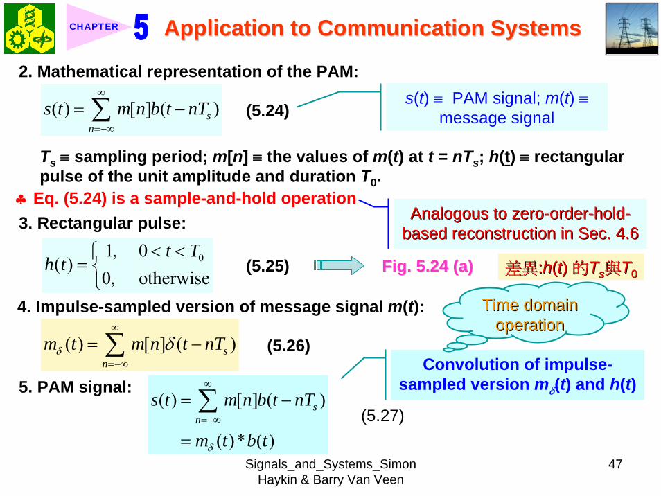
Signals_and_Systems_Simon Haykin amp Barry Van Veen
47
Application to Communication SystemsApplication to Communication SystemsCHAPTER
2 Mathematical representation of the PAM
( ) [ ] ( )sn
s t m n b t nTinfin
=minusinfin
= minussum (524) s(t) equiv PAM signal m(t) equiv
message signal
Ts equiv sampling period m[n] equiv the values of m(t) at t = nTs h(t) equiv rectangular pulse of the unit amplitude and duration T0
3 Rectangular pulse
01 0( )
0 otherwiset T
h tlt lt⎧
= ⎨⎩
(525) Fig 524 (a)Fig 524 (a)
clubs Eq (524) is a sample-and-hold operationAnalogous to zeroAnalogous to zero--orderorder--holdhold--
based reconstruction in Sec 46based reconstruction in Sec 46
差異差異hh((tt) ) 的的TTss與與TT00
4 Impulse-sampled version of message signal m(t)
( ) [ ] ( )sn
m t m n t nTδ δinfin
=minusinfin
= minussum (526)
5 PAM signal( ) [ ] ( )
( ) ( )
sn
s t m n b t nT
m t b tδ
infin
=minusinfin
= minus
=
sum(527)
Convolution of impulse-sampled version mδ(t) and h(t)
Time domain Time domain operationoperation
Signals_and_Systems_Simon Haykin amp Barry Van Veen
48
Application to Communication SystemsApplication to Communication SystemsCHAPTER
Figure 524 (p 453)(a) Rectangular pulse h(t) of unit amplitude and duration T0 (b) Magnitude spectrum |H(jω)| and phase spectrum argH(jω) of pulse h(t)
v equiv ω p equiv π
Signals_and_Systems_Simon Haykin amp Barry Van Veen
49
Application to Communication SystemsApplication to Communication SystemsCHAPTER
6 FT of PAM signal( ) ( ) ( )S j M j H jδω ω ω= (528)
where( ) ( )FTS j s tω larr⎯rarr ( ) ( )FTM j m tδ δω larr⎯rarr ( ) ( )FTH j h tω larr⎯rarr
7 Impulse sampling of the message signal m(t) introduces periodicity into the spectrum as given by
1( ) ( ( ))sks
M j M j kTδ ω ω ω
infin
=minusinfin
= minussum (529) 1Ts equiv sampling rate ωs = 2πTs rads
1( ) ( ( )) ( )sks
S j M j k H jT
ω ω ω ωinfin
=minusinfin
= minussum (530)
( ) ( )FTM j m tω larr⎯rarrwhere
clubs Suppose that m(t) is strictly band limited and that the sampling rate 1Ts is greater than the Nyquist rate Then passing s(t) through a reconstruction filter chosen as an ideal low-pass filter with cutoff frequency ωm and gain Ts we find that the spectrum of the resulting filter output is equal to M(jω)H(jω)
Signals_and_Systems_Simon Haykin amp Barry Van Veen
50
Application to Communication SystemsApplication to Communication SystemsCHAPTER
8 From Eq (525) we find that0 2
0 0( ) sin ( (2 )) j TH j T c T e ωω ω π minus= (531) Fig 524(b) magnitude and phase of H(jω)
clubs Using PAM to represent a continuous-time message signal we introduce amplitude distortion as well as a delay of T02
clubs The frequency distortion caused by the use of flat-topped sampled in the generation of a PAM wave illustrated in Fig 523Fig 523 is referred to as the aperture effect
583 583 Demodulation of PAM SignalDemodulation of PAM Signal1 Reconstruction scheme Fig 525Fig 525
Figure 525 (p 454)Figure 525 (p 454)System consisting of low-pass interpolation filter and equalizer for reconstructing a message signal from its flattopped sampled version
clubs The system consists of low-pass interpolation filter and equalizer connected in cascade
Signals_and_Systems_Simon Haykin amp Barry Van Veen
51
Application to Communication SystemsApplication to Communication SystemsCHAPTER
2 The cutoff frequency of low-pass filter = the highest frequency ωm of message signal
3 The equalizer is used to correct the aperture effect due to flat-topped sampling in the sample-and-hold circuit
4 The equalizer has the effect of decreasing the in-band loss of the interpolation filter as frequency increases in such a manner as to compensate for the aperture effect
5 Amplitude response of equalizer
0
0 0 0 0
1 1 1| ( ) | | sinc( 2) | 2 | sin( 2) |
TH j T T T T
ωω ω ω
= =
Frequency response Eq (531)
Example 55 Equalization for PAM TransmissionThe duty cycle in a PAM signal namely T0 Ts is 10 Evaluate the peak amplification required for equalizationltltSolgtSolgt1 At ωm = π Ts which corresponds to the highest frequency component of the
message signal for a sampling rate equal to the Nyquist rate we find from Eq (531) that the magnitude response of the equalizer at ωm normalized to that at zero frequency is
Signals_and_Systems_Simon Haykin amp Barry Van Veen
52
Application to Communication SystemsApplication to Communication SystemsCHAPTER
Figure 526 (p 455)Figure 526 (p 455)Normalized equalization (to compensate for aperture effect) plotted against the duty cycle T0Ts
Signals_and_Systems_Simon Haykin amp Barry Van Veen
53
Application to Communication SystemsApplication to Communication SystemsCHAPTER
0
0 0
( 2)( )1sin (05 ) sin[( 2)( )]
s
s s
T Tc T T T T
ππ
=
where the ratio T0 Ts is equal to the duty cycle of the sampling pulses 2 In Fig 526Fig 526 this result is plotted as a function of the duty cycle T0 Ts Ideally it
should be equal to unity for all values of T0 Ts 3 For a duty cycle of 10 it is equal to 10041 It follows that for duty cycles of less
than 10 the magnitude equalization required is less than 10041 in which case the aperture effect is usually considered to be negligible
59 59 Multiplexing Multiplexing clubs Three basic types of multiplexing1 Frequency-division multiplexing in which the signals are separated by
allocating them to different frequency bands This is illustrated in Fig 527(a) for the case of six different message signals Frequency-division multiplexing favors the use of CW modulation where each message signal is able to use the channel on a continuous-time basis
2 Time-division multiplexing wherein the signals are separated by allocating them to different time slots within a sampling interval
Signals_and_Systems_Simon Haykin amp Barry Van Veen
54
Application to Communication SystemsApplication to Communication SystemsCHAPTER
This second type of multiplexing is illustrated in Fig 527(b) for the case of six different message signals Code-division multiplexing which relies on the assignment of different codes to the individual users of the channel
3 Code-division multiplexing which relies on the assignment of different codes to the individual users of the channel
591 591 FrequencyFrequency--Domain Multiplexing (FDM)Domain Multiplexing (FDM)1 Block diagram Fig 528Fig 5282 Incoming message signals low-pass variety3 Low-pass filter to remove high-frequency components such that the signal
in each channel does not disturb each other4 MOD (modulator) shift the frequency ranges of the signals so as to occupy
mutually exclusive frequency intervalsSSB is often used in this stageEx Voice input is usually assigned a bandwidth of 4 kHz
5 Band-pass filters are used to restrict the band of each modulated wave to its prescribed range
6 Band-pass filters in receiver separate the message signals7 DEM (demodulator) to recover signalsclubs FDM in Fig 528 operates in only one direction
Signals_and_Systems_Simon Haykin amp Barry Van Veen
55
Application to Communication SystemsApplication to Communication SystemsCHAPTER
Figure 527 (p 456)Figure 527 (p 456)Two basic forms of multiplexing (a) Frequency-division multiplexing (with guardbands) (b) Time-division multiplexing no provision is made here for synchronizing pulses
Signals_and_Systems_Simon Haykin amp Barry Van Veen
56
Application to Communication SystemsApplication to Communication SystemsCHAPTER
Figure 528 (p 457)Figure 528 (p 457)Block diagram of FDM system showing the important constituents of the transmitter and receiver
Signals_and_Systems_Simon Haykin amp Barry Van Veen
57
Application to Communication SystemsApplication to Communication SystemsCHAPTER
Example 56 SSB-FDM System
ltltSolgtSolgt
An FDM system is used to multiplex 24 independent voice signals SSB modulation is used for the transmission Given that each voice signal is allotted a bandwidth 4kHz calculate the overall transmission bandwidth of the channel
With each voice signal allotted a bandwidth of 4 kHz the use of SSB modulation requires a bandwidth of 4 kHz for its transmission Accordingly the overall transmission bandwidth provided by the channel is 24 X 4 = 96 kHz 592 592 TimeTime--Domain Multiplexing (TDM)Domain Multiplexing (TDM)clubs Basic to the operation of a TDM system is the sampling theoremclubs The transmission of the message samples engages the transmission channel for
only a fraction of the sampling interval on a periodic basis equal to the width T0 of a PAM modulating pulse
1 Block diagram Fig 529Fig 5292 Commutator is usually implemented by means of electronic switching
circuitry3 The function of commutator is two folds
Signals_and_Systems_Simon Haykin amp Barry Van Veen
58
Application to Communication SystemsApplication to Communication SystemsCHAPTER
Figure 529 (p 458)Figure 529 (p 458)Block diagram of TDM system showing the important constituents of the transmitter and receiver
(1) To take a narrow sample of each of the M input message signals at a rate 1Tsthat is slightly higher than ωcπ where ωc is the cutoff frequency of the input low-pass filter
(2) To sequentially interleave these M samples inside a sampling interval Ts4 Pulse modulator transform the multiplexed signal into a form suitable for
transmission over the common channel
Signals_and_Systems_Simon Haykin amp Barry Van Veen
59
Application to Communication SystemsApplication to Communication SystemsCHAPTER
clubs The use of time-division multiplexing introduces a bandwidth expansion factor M because the scheme must squeeze M samples derived from M independent message sources into a time slot equal to one sampling interval
5 Pulse demodulator performs the inverse operation of the pulse modulator6 Decommutator distributes the narrow samples produced by pulse demodulator to the appropriate low-pass reconstruction filter7 Synchronization between the timing operations of the transmitter and
receiver in a TDM system is essential for satisfactory performance of the system
Inserting an extra pulse into each sampling interval on a regular basisBandwidth expansion factor is increased to M + 1
clubs The TDM system is hghly sensitive to the dispersion in the common transmission channel
Example 57 Comparison of TDM with FDMATDM system is used to multiplex four independent voice signals using PAM Each voice signal is sampled at the rate of 8 kHz The system incorporates a synchronizing pulse train for its proper operation
Signals_and_Systems_Simon Haykin amp Barry Van Veen
60
Application to Communication SystemsApplication to Communication SystemsCHAPTER
(a) Determine the timing relationships between the synchronizing pulse train and the impulse trains used to sample the four voice signals
(b) Calculate the transmission bandwidth of the channel for the TDM system and compare the result with a corresponding FDM system using SSBmodulation
ltltSolgtSolgt(a) The sampling period is
31 125 s
8 10sT s μ= =times
In this example the number of voice signals is M = 4 Hence dividing the sampling period of 125 μs among these voice signals and the synchronizing pulse train we obtain the time slot allocated to each one of them
0 1125 25 s
5
sTTM
μ
=+
= =
Signals_and_Systems_Simon Haykin amp Barry Van Veen
61
Application to Communication SystemsApplication to Communication SystemsCHAPTER
Figure 530Figure 530 shows the timing relationships between the synchronizing pulse train and the four impulse trains used to sample the different voice signals in a single frame Each frame includes time slots of common duration T0 = 25 μs which are allocated to the pulse-modulated signals and synchronizing pulse
Figure 530 (p 459)Figure 530 (p 459)Composition of one frame of a multiplexed PAM signal incorporating four voice-signals and a synchronizing pulse
Signals_and_Systems_Simon Haykin amp Barry Van Veen
62
Application to Communication SystemsApplication to Communication SystemsCHAPTER
(b) As a consequence of the time-bandwidth product (see Section 317) there is an inverse relationship between the duration of a pulse and the bandwidth (ie cutoff frequency) of the channel needed for itstransmission Accordingly the overall transmission bandwidth of the channel is
0
21 1 MHz 40 kHz
25
TTf
T
ωπ
=
= = =
In contrast the use of an FDM system based on SSB modulation requires a channel bandwidth equal to M times that of a single voice signal-that is 4 X 4 = 16 kHz Thus the use of PAM-TDM requires a channel bandwidth that is 40 16 = 25 times that of SSB-FDMIn practice pulse-code modulation is commonly used as the method of modulation for TDM this results in a further increase in channel bandwidth depending on the length of the code word used in the digital representation of each pulse in the PAM signal
Signals_and_Systems_Simon Haykin amp Barry Van Veen
63
Application to Communication SystemsApplication to Communication SystemsCHAPTER
510 510 Pulse and Group Delays Pulse and Group Delays 1 Whenever a signal is transmitted through a dispersive (ie frequency
selective) system some delay is introduced into the output signal in relation to the input signal
2 The delay is determined by the phase response of the system3 Phase response of a dispersive communication channel
( ) arg ( )H jφ ω ω= (532)
A signal is transmitted through the channel at a frequency ωc The signal received at the channel lags the transmitted signal by φ(ωc) The time delay is called phase delay formally defined as
( )cp
c
φ ωτω
= minus (533)
The phase delay is not necessarily the true signal delayclubs Case study for DSB-SC1 Transmitted signal
0( ) cos( ) cos( )cs t A t tω ω= (534)
ωc equiv carrier frequency ω0 equiv sinusoidal modulation frequency
A = AcA0
Signals_and_Systems_Simon Haykin amp Barry Van Veen
64
Application to Communication SystemsApplication to Communication SystemsCHAPTER
1 21 1( ) cos( ) cos( )2 2
s t A t A tω ω= +
1 0cω ω ω= + (535) where
2 0cω ω ω= minus (536)
Upper frequency
Lower frequency
2 Let the s(t) be transmitted through the channel with phase response φ (ω) Accordingly the signal received at the channel output is
1 1 2 21 1( ) cos( ( )) cos( ( ))2 2
y t A t A tω φ ω ω φ ω= + + +
1 2 1 20
( ) ( ) ( )1 ( )( ) cos cos2 2cy t A t tφ ω φ ω φ ω φ ωω ω+⎛ ⎞ ⎛ ⎞= + +⎜ ⎟ ⎜ ⎟
⎝ ⎠ ⎝ ⎠(537)
3 Two observations from Eq (537)1) The carrier component at frequency ωc in y(t) lags its counterpart in s(t) by
frac12 (φ (ω1) + φ (ω2)) which represents a time delay equal to
1 2 1 2
c 1 2
( )+ ( ) ( )+ ( )2 +
φ ω φ ω φ ω φ ωω ω ω
minus = minus (538)
Signals_and_Systems_Simon Haykin amp Barry Van Veen
65
Application to Communication SystemsApplication to Communication SystemsCHAPTER
2) The message component at frequency ω0 in y(t) lags its counterpart in s(t) by frac12 (φ (ω1) minus φ (ω2)) which represents a time delay equal to
1 2 1 2
0 1 2
( ) ( ) ( ) ( )2
φ ω φ ω φ ω φ ωω ω ωminus minus
minus = minusminus
(539)
4 Suppose that ω0 lt ωc rArr the side frequencies are close together with ω c between them Such a modulated signal is said to be a narrowband signal The phase response φ (ω) in the vicinity of ω = ωc is approximated by two-term Taylor series expansion
( )( ) ( ) ( )c
c cd
d ω ω
φ ωφ ω φ ω ω ωω =
= + times minus (540)
Phase delay = ( ) c cφ ω ωminus
5 The time delay introduced by the message signal (ie he ldquoenveloperdquo of the modulated signal) is given by
( )
c
gd
d ω ω
φ ωτω =
= minus (541) The time delay τg is called the
envelope delay or group delay
Signals_and_Systems_Simon Haykin amp Barry Van Veen
66
Application to Communication SystemsApplication to Communication SystemsCHAPTER
6 When a modulated signal is transmitted through a communication channel there are two different delays to be considered1) The carrier or phase delay τp defined by Eq (533)2) The envelope or group delay τg defined by Eq (541)
clubs The group delay is the true signal delay
Example 58 Phase and Group Delays for Ban-pass Channel
ltltSolgtSolgt
The phase response of a band-pass communication channel is defined by 2 2
1( ) tan c
c
ω ωφ ωωω
minus ⎛ ⎞minus= minus ⎜ ⎟
⎝ ⎠The signal s(t) defined in Eq (534) is transmitted through this channel with
475 radscω = 0 025 radsω =andCalculate (a) the phase delay and (b) the group delay
(a) At ω = ωc φ (ωc) = 0 According to Eq (533) the phase delay τ p is zero (b) Differentiating φ (ω) with respect to ω we get
Signals_and_Systems_Simon Haykin amp Barry Van Veen
67
Application to Communication SystemsApplication to Communication SystemsCHAPTER
2 2
2 2 2 2 2
( )( )( )
c c
c c
dd
ω ω ωφ ωω ω ω ω ω
+= minus
+ minus
Using thing result in Eq (541) we find that the group delay is 2 2 04211
475gc
sτω
= = =
1 One waveform shown as a solid curve was obtained by multiplying the transmitted signal s(t) by the carrier wave cos(ωct)
2 The second waveform shown as a dotted curve was obtained by multiplying the received signal y(t) by the carrier wave cos(ωct)
To display the results obtained in parts (a) and (b) in graphical form Fig 531Fig 531shows a superposition of two waveforms obtained as follows
The figure clearly shows that the carrier (phase) delay τ p is zero and the envelope of the received signal y(t) is lagging behind that of the transmitted signal by τs seconds For the presentation of waveforms in this figure we purposely did not use a filter to suppress the high frequency components resulting from the multiplications described under points 1 and 2 because of the desire to retain a contribution due to the carrier for display
Signals_and_Systems_Simon Haykin amp Barry Van Veen
68
Application to Communication SystemsApplication to Communication SystemsCHAPTER
Figure 531 Figure 531 (p 463)(p 463)Highlighting the zero carrier delay (solid curve) and group delay τg (dotted curve) which are determined in accordance with Example 58
Signals_and_Systems_Simon Haykin amp Barry Van Veen
69
Application to Communication SystemsApplication to Communication SystemsCHAPTER
clubs Not also that the separation between the upper side frequency ω1 = ωc + ω0 = 500 rads and the lower side frequency ω2 = ωc minus ω0 = 450 rads is about 10 of the carrier frequency ωc = 475 rads which justifies referring to the modulated signal in this example as a narrowband signal
5101 5101 Some Practical ConsiderationsSome Practical Considerationsclubs What is the practical importance of group delay 1 Eq (541) for determining group delay applies strictly to narrowband
modulated signal2 The message bandwidth may be comparable to the carrier frequency In
this situation the group delay is formulated as a frequency-dependent parameter ie ( )d( )g d
φ ωτ ωω
= minus (542)
3 When a wideband modulated signals transmitted through a dispersive channel the frequency components of the message signal are delayed by different amounts at the channel output
Delay distortionFig 532Fig 532 Group delay response of voice-grade telephone channel
Signals_and_Systems_Simon Haykin amp Barry Van Veen
70
Application to Communication SystemsApplication to Communication SystemsCHAPTER
Figure 532 (p 464)Group delay response of voice-grade telephone channel (Adapted from J C Bellamy Digital Telephony Wiley 1982)
511 511 Exploring Concepts with MATLABExploring Concepts with MATLAB5111 5111 Full AMFull AMclubs Sinusoidal modulation
clubs To reconstruct a faithful version of the original message signal in the receiver we have to use a delay equalizer
0( ) [1 cos( )]cos( )c cs t A t tμ ω ω= +1 AM experiment
1cA =
08 radscω π= 0 01 radsω π=Carrier amplitude
Carrier frequency Modulation amplitude
Signals_and_Systems_Simon Haykin amp Barry Van Veen
71
Application to Communication SystemsApplication to Communication SystemsCHAPTER
2 We wish to display and analyze 10 full cycles of the AM wave corresponding to a total duration of 200 s Choosing a sampling rate 1Ts = 10 Hz we have a total of N = 2000 time samples The frequency band of interest is minus 10 π ≦ ω ≦ 10 π Since the separation between the carrier and either side frequency is equal to the modulation frequency ω0 = 01 π rads we would like to have a frequency resolution ωr = 001π rads To achieve this resolution we require the following number of frequency samples (see Eq (442))
20 2000001
s
r
M ω πω π
ge = =
3 We therefore choose M = 2000 To approximate the Fourier transform of the AM wave s(t) we may use a 2000-point DTFS The only variable in the AM experiment is the modulation factor μ with respect to which we wish to investigate three different situationsμ = 05 corresponding to under-modulationμ = 10 for which the AM system is on the verge of over-modulationμ = 20 corresponding to over-modulation
Signals_and_Systems_Simon Haykin amp Barry Van Veen
72
Application to Communication SystemsApplication to Communication SystemsCHAPTER
4 MATLAB commandsAc = 1 carrier amplitudewc = 08pi carrier frequencyw0 = 01pi modulation frequencymu = 05 modulation factort = 0011999s = Ac(1 + mucos(w0t))cos(wct)plot(ts)Smag = abs(fftshift(fft(s2000)))2000 Smag denotes the magnitude specturm of the AM wavew = 10[-1000999]2pi2000plot(wSmag)axis ([-30 30 0 08])
5 5 μμ = 05 = 05 case case Fig 533Fig 533μμ = 10 case = 10 case Fig 534Fig 534μμ = 20 case = 20 case Fig 535Fig 535
Discussion see pp 466-469 textbook
Signals_and_Systems_Simon Haykin amp Barry Van Veen
73
Application to Communication SystemsApplication to Communication SystemsCHAPTER
-30 -20 -10 0 10 20 300
02
04
06
0 50 100 150 200-2
-1
0
1
2
2 22 24 26 28 3
02
04
06
(a) Time (s)
Time domain
Frequency domain
(b) Frequency (rads)
Frequency domain
Frequency (rads)
Figure 533 (p 466)Amplitude modulation with 50 modulation (a) AM wave (b) magnitude spectrum of the AM wave and (c) expanded spectrum around the carrier frequency
μμ = 05 = 05 casecase
Signals_and_Systems_Simon Haykin amp Barry Van Veen
74
Application to Communication SystemsApplication to Communication SystemsCHAPTER
Figure 534 (p 467)Figure 534 (p 467)Amplitude modulation with 100 modulation (a) AM wave (b) magnitude spectrum of the AM wave and (c) expanded spectrum around the carrier frequency
Signals_and_Systems_Simon Haykin amp Barry Van Veen
75
Application to Communication SystemsApplication to Communication SystemsCHAPTER
Figure 535 (p 468)Amplitude modulation with 200 modulation (a) AM wave (b) magnitude spectrum of the AM wave and (c) expanded spectrum around the carrier frequency
Signals_and_Systems_Simon Haykin amp Barry Van Veen
76
Application to Communication SystemsApplication to Communication SystemsCHAPTER
5112 5112 DSBDSB--SC ModulationSC Modulation1 Sinusoidal modulation
0 0( ) cos( ) cos( )c cs t A A t tω ω=
2 MATLAB commands
Ac = 1 carrier amplitudewc = 08pi carrier frequency in radsA0 = 1 amplitude of modulating signalw0 = 01pi frequency of modulating signalt = 011999s = AcA0cos(wct)cos(w0t)plot(ts)Smag = abs(fftshift(fft(s2000)))2000w = 10[-1000999]2pi2000plot(wSmag)
3 3 DSBDSB--SC modulated waveSC modulated wave Fig 536Fig 536 Discussion see pp 466-469 textbook
4 Output of the product modulator in Fig 512 (b) with φ = 0
Signals_and_Systems_Simon Haykin amp Barry Van Veen
77
Application to Communication SystemsApplication to Communication SystemsCHAPTER
Figure 536 (p 469)DSB-SC modulation (a) DSB-SC modulated wave (b) magnitude spectrum of the modulated wave and (c) expanded spectrum around the carrier frequency
Signals_and_Systems_Simon Haykin amp Barry Van Veen
78
Application to Communication SystemsApplication to Communication SystemsCHAPTER
( ) ( ) cos( )cv t s t tω=
5 MATLAB commandsgtgt v = scos(wct)
6 Fig 537 (a) waveforms of v(t) Fig 537 (b) magnitude spectrum which readily shows that v(t) consists of the following components1) A sinusoidal component with frequency 01π rads representing the
modulating wave2) A new DSB-SC modulated wave with double carrier frequency of 16π rads
in actuality the side frequencies of this modulated wave are located at 15πand 17π rads
1) The frequency of the modulating wave lies inside the passband of the filter2) The upper and lower side frequencies of the new DSB-SC modulated wave
lie inside the stopband of the filter
Accordingly we may recover the sinusoidal modulating signal by passing v(t) through low-pass filter with the following requirements
Signals_and_Systems_Simon Haykin amp Barry Van Veen
79
Application to Communication SystemsApplication to Communication SystemsCHAPTER
Figure 537 (p 470)Coherent detection of DSB-SC modulated wave (a) and (b) Waveform and magnitude spectrum of signal produced at the output of produce modulator (c) and (d) waveform and magnitude spectrum of low-pass filter output
Signals_and_Systems_Simon Haykin amp Barry Van Veen
80
Application to Communication SystemsApplication to Communication SystemsCHAPTER
The issue of how to design a filter with these requirements will be considered in detail in Chapter 8 For the present it suffices to say that the preceding requirements can be met by using the following MATLAB commands
gtgt [ba] = butter(30025)gtgt output = filter(bav)
The first command produces s special type of filter called a Butterworth filter For the experiment considered here the filter order is 3 and its normalized cutoff frequency of 0025 is calculated as follows
Actual cutoff frequency of filter 025 radsHalf the sampling rate 10 rads
0025
ππ
=
=
The second command computes the filterrsquos output in response to the product modulator output v(t) (We will revisit the design of this filter in Chapter 8) Figure 537(c) displays the waveform of the low-pass filter output this waveform represents a sinusoidal signal of frequency 005 Hz an observation that is confirmed by using the ffr command to approximate the spectrum of the filter output The result of the computation is shown in Fig 537(d)Fig 537(d)
Signals_and_Systems_Simon Haykin amp Barry Van Veen
81
Application to Communication SystemsApplication to Communication SystemsCHAPTER
7 In Fig 538 we explore another aspect of DSB-SC modulation namely the effect of varying the modulation frequency Figure 538(a) shows five cycles of a DSB-SC modulated wave that has the same carrier frequency as that in Fig 536(a) but the modulation frequency has been reduced to 0025 Hz( ie a radian frequency of 005π) Figure 538(b) shows the magnitude spectrum of this second DSB-SC modulated wave and its zoomed-in version is shown in Fig 538(c) Comparing this latter figure with Fig 536(c) we see clearly that decreasing the modulation frequency has the effect of moving the upper and lower side frequencies closer together which is consistent with modulation theory
5113 5113 Phase and Group DelayPhase and Group Delay1 In Example 58 we studied the phase and group delays for a band-pass
channel with phase response 2 2
1( ) tan c
c
ω ωφ ωωω
minus ⎛ ⎞minus= minus ⎜ ⎟
⎝ ⎠2 At ω = ωc the phase delay is τ p = 0 and the group delay is τ s = 04211s One
of the wave forms displayed in Fig 531Fig 531 is
1( ) ( ) cos( )cx t s t tω=
Signals_and_Systems_Simon Haykin amp Barry Van Veen
82
Application to Communication SystemsApplication to Communication SystemsCHAPTER
Figure 538 (p 472)Effect of varying the modulation frequency compared with that in Fig 537 (a) and (b) Waveform and magnitude spectrum of DSB-SC modulated wave with a modulation frequency one-half that used in Fig 536 (c) expanded spectrum around the carrier frequency
Signals_and_Systems_Simon Haykin amp Barry Van Veen
83
Application to Communication SystemsApplication to Communication SystemsCHAPTER
where (see page 461)
1 2( ) [cos( ) cos( )]2As t t tω ω= +
and ω1 = ωc + ω0 and ω2 = ωc - ω0 The waveform shown in the figure as a solid curve is a plot of x1(t) The other waveform also displayed in Fig 531Fig 531 is
2
1 1 2 2
( ) ( ) cos( )
[cos( ( )) cos( ( ))]cos( )2
c
c
x t y t tA t t t
ω
ω φ ω ω φ ω ω
=
= + + +
where the angle φ (ω1) and φ (ω2) are the values of the phase response φ (ω) at ω = ω1 and ω = ω2 respectively The waveform shown as a dotted curve in the figure is a plot of x2(t)
3 The generation of x1(t) and x2(t) in MATLAB is achieved with the following commands with A2 set equal to unity
Signals_and_Systems_Simon Haykin amp Barry Van Veen
84
Application to Communication SystemsApplication to Communication SystemsCHAPTER
wc = 475w0 = 025w1 = wc + w0w2 = wc - w0t = -10 0001 10o1 = -atan((w1^2 - wc^2)(w1wc))o2 = -atan((w2^2 - wc^2)(w2wc))s = cos(w1t) + cos(w2t)y = cos(w1t + o1) + cos(w2t + o2)x1 = scos(478t)x2 = ycos(475t)plot(tx1b)hold on plot(tx2k)hold offxlabel(Time)ylabel(Amplitude)
Note that we have set (A2) = 1 for convenience of presentation The function atan in the first two commands returns the arctangent Note also that the computation of both x1 and x2 involve element-by-element multiplications ndash hence the use of period followed by an asterisk
Signals_and_Systems_Simon Haykin amp Barry Van Veen
85
Application to Communication SystemsApplication to Communication SystemsCHAPTER
Signals_and_Systems_Simon Haykin amp Barry Van Veen
86
Application to Communication SystemsApplication to Communication SystemsCHAPTER
Signals_and_Systems_Simon Haykin amp Barry Van Veen
87
Application to Communication SystemsApplication to Communication SystemsCHAPTER
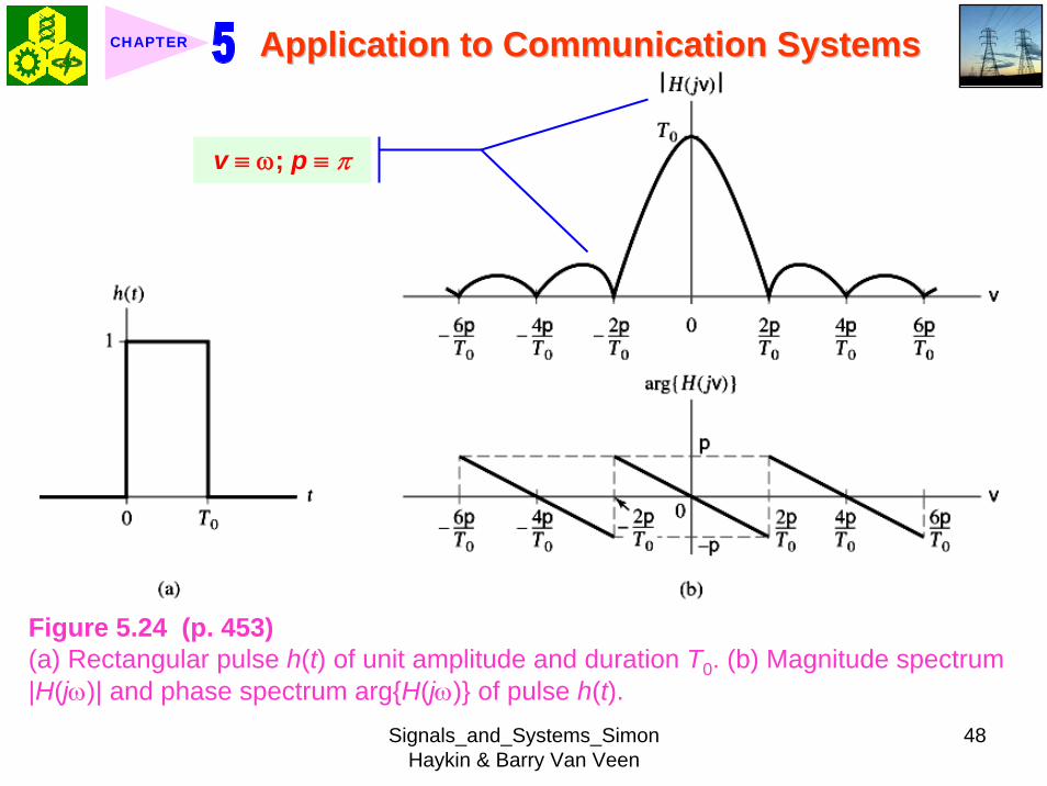
Signals_and_Systems_Simon Haykin amp Barry Van Veen
48
Application to Communication SystemsApplication to Communication SystemsCHAPTER
Figure 524 (p 453)(a) Rectangular pulse h(t) of unit amplitude and duration T0 (b) Magnitude spectrum |H(jω)| and phase spectrum argH(jω) of pulse h(t)
v equiv ω p equiv π
Signals_and_Systems_Simon Haykin amp Barry Van Veen
49
Application to Communication SystemsApplication to Communication SystemsCHAPTER
6 FT of PAM signal( ) ( ) ( )S j M j H jδω ω ω= (528)
where( ) ( )FTS j s tω larr⎯rarr ( ) ( )FTM j m tδ δω larr⎯rarr ( ) ( )FTH j h tω larr⎯rarr
7 Impulse sampling of the message signal m(t) introduces periodicity into the spectrum as given by
1( ) ( ( ))sks
M j M j kTδ ω ω ω
infin
=minusinfin
= minussum (529) 1Ts equiv sampling rate ωs = 2πTs rads
1( ) ( ( )) ( )sks
S j M j k H jT
ω ω ω ωinfin
=minusinfin
= minussum (530)
( ) ( )FTM j m tω larr⎯rarrwhere
clubs Suppose that m(t) is strictly band limited and that the sampling rate 1Ts is greater than the Nyquist rate Then passing s(t) through a reconstruction filter chosen as an ideal low-pass filter with cutoff frequency ωm and gain Ts we find that the spectrum of the resulting filter output is equal to M(jω)H(jω)
Signals_and_Systems_Simon Haykin amp Barry Van Veen
50
Application to Communication SystemsApplication to Communication SystemsCHAPTER
8 From Eq (525) we find that0 2
0 0( ) sin ( (2 )) j TH j T c T e ωω ω π minus= (531) Fig 524(b) magnitude and phase of H(jω)
clubs Using PAM to represent a continuous-time message signal we introduce amplitude distortion as well as a delay of T02
clubs The frequency distortion caused by the use of flat-topped sampled in the generation of a PAM wave illustrated in Fig 523Fig 523 is referred to as the aperture effect
583 583 Demodulation of PAM SignalDemodulation of PAM Signal1 Reconstruction scheme Fig 525Fig 525
Figure 525 (p 454)Figure 525 (p 454)System consisting of low-pass interpolation filter and equalizer for reconstructing a message signal from its flattopped sampled version
clubs The system consists of low-pass interpolation filter and equalizer connected in cascade
Signals_and_Systems_Simon Haykin amp Barry Van Veen
51
Application to Communication SystemsApplication to Communication SystemsCHAPTER
2 The cutoff frequency of low-pass filter = the highest frequency ωm of message signal
3 The equalizer is used to correct the aperture effect due to flat-topped sampling in the sample-and-hold circuit
4 The equalizer has the effect of decreasing the in-band loss of the interpolation filter as frequency increases in such a manner as to compensate for the aperture effect
5 Amplitude response of equalizer
0
0 0 0 0
1 1 1| ( ) | | sinc( 2) | 2 | sin( 2) |
TH j T T T T
ωω ω ω
= =
Frequency response Eq (531)
Example 55 Equalization for PAM TransmissionThe duty cycle in a PAM signal namely T0 Ts is 10 Evaluate the peak amplification required for equalizationltltSolgtSolgt1 At ωm = π Ts which corresponds to the highest frequency component of the
message signal for a sampling rate equal to the Nyquist rate we find from Eq (531) that the magnitude response of the equalizer at ωm normalized to that at zero frequency is
Signals_and_Systems_Simon Haykin amp Barry Van Veen
52
Application to Communication SystemsApplication to Communication SystemsCHAPTER
Figure 526 (p 455)Figure 526 (p 455)Normalized equalization (to compensate for aperture effect) plotted against the duty cycle T0Ts
Signals_and_Systems_Simon Haykin amp Barry Van Veen
53
Application to Communication SystemsApplication to Communication SystemsCHAPTER
0
0 0
( 2)( )1sin (05 ) sin[( 2)( )]
s
s s
T Tc T T T T
ππ
=
where the ratio T0 Ts is equal to the duty cycle of the sampling pulses 2 In Fig 526Fig 526 this result is plotted as a function of the duty cycle T0 Ts Ideally it
should be equal to unity for all values of T0 Ts 3 For a duty cycle of 10 it is equal to 10041 It follows that for duty cycles of less
than 10 the magnitude equalization required is less than 10041 in which case the aperture effect is usually considered to be negligible
59 59 Multiplexing Multiplexing clubs Three basic types of multiplexing1 Frequency-division multiplexing in which the signals are separated by
allocating them to different frequency bands This is illustrated in Fig 527(a) for the case of six different message signals Frequency-division multiplexing favors the use of CW modulation where each message signal is able to use the channel on a continuous-time basis
2 Time-division multiplexing wherein the signals are separated by allocating them to different time slots within a sampling interval
Signals_and_Systems_Simon Haykin amp Barry Van Veen
54
Application to Communication SystemsApplication to Communication SystemsCHAPTER
This second type of multiplexing is illustrated in Fig 527(b) for the case of six different message signals Code-division multiplexing which relies on the assignment of different codes to the individual users of the channel
3 Code-division multiplexing which relies on the assignment of different codes to the individual users of the channel
591 591 FrequencyFrequency--Domain Multiplexing (FDM)Domain Multiplexing (FDM)1 Block diagram Fig 528Fig 5282 Incoming message signals low-pass variety3 Low-pass filter to remove high-frequency components such that the signal
in each channel does not disturb each other4 MOD (modulator) shift the frequency ranges of the signals so as to occupy
mutually exclusive frequency intervalsSSB is often used in this stageEx Voice input is usually assigned a bandwidth of 4 kHz
5 Band-pass filters are used to restrict the band of each modulated wave to its prescribed range
6 Band-pass filters in receiver separate the message signals7 DEM (demodulator) to recover signalsclubs FDM in Fig 528 operates in only one direction
Signals_and_Systems_Simon Haykin amp Barry Van Veen
55
Application to Communication SystemsApplication to Communication SystemsCHAPTER
Figure 527 (p 456)Figure 527 (p 456)Two basic forms of multiplexing (a) Frequency-division multiplexing (with guardbands) (b) Time-division multiplexing no provision is made here for synchronizing pulses
Signals_and_Systems_Simon Haykin amp Barry Van Veen
56
Application to Communication SystemsApplication to Communication SystemsCHAPTER
Figure 528 (p 457)Figure 528 (p 457)Block diagram of FDM system showing the important constituents of the transmitter and receiver
Signals_and_Systems_Simon Haykin amp Barry Van Veen
57
Application to Communication SystemsApplication to Communication SystemsCHAPTER
Example 56 SSB-FDM System
ltltSolgtSolgt
An FDM system is used to multiplex 24 independent voice signals SSB modulation is used for the transmission Given that each voice signal is allotted a bandwidth 4kHz calculate the overall transmission bandwidth of the channel
With each voice signal allotted a bandwidth of 4 kHz the use of SSB modulation requires a bandwidth of 4 kHz for its transmission Accordingly the overall transmission bandwidth provided by the channel is 24 X 4 = 96 kHz 592 592 TimeTime--Domain Multiplexing (TDM)Domain Multiplexing (TDM)clubs Basic to the operation of a TDM system is the sampling theoremclubs The transmission of the message samples engages the transmission channel for
only a fraction of the sampling interval on a periodic basis equal to the width T0 of a PAM modulating pulse
1 Block diagram Fig 529Fig 5292 Commutator is usually implemented by means of electronic switching
circuitry3 The function of commutator is two folds
Signals_and_Systems_Simon Haykin amp Barry Van Veen
58
Application to Communication SystemsApplication to Communication SystemsCHAPTER
Figure 529 (p 458)Figure 529 (p 458)Block diagram of TDM system showing the important constituents of the transmitter and receiver
(1) To take a narrow sample of each of the M input message signals at a rate 1Tsthat is slightly higher than ωcπ where ωc is the cutoff frequency of the input low-pass filter
(2) To sequentially interleave these M samples inside a sampling interval Ts4 Pulse modulator transform the multiplexed signal into a form suitable for
transmission over the common channel
Signals_and_Systems_Simon Haykin amp Barry Van Veen
59
Application to Communication SystemsApplication to Communication SystemsCHAPTER
clubs The use of time-division multiplexing introduces a bandwidth expansion factor M because the scheme must squeeze M samples derived from M independent message sources into a time slot equal to one sampling interval
5 Pulse demodulator performs the inverse operation of the pulse modulator6 Decommutator distributes the narrow samples produced by pulse demodulator to the appropriate low-pass reconstruction filter7 Synchronization between the timing operations of the transmitter and
receiver in a TDM system is essential for satisfactory performance of the system
Inserting an extra pulse into each sampling interval on a regular basisBandwidth expansion factor is increased to M + 1
clubs The TDM system is hghly sensitive to the dispersion in the common transmission channel
Example 57 Comparison of TDM with FDMATDM system is used to multiplex four independent voice signals using PAM Each voice signal is sampled at the rate of 8 kHz The system incorporates a synchronizing pulse train for its proper operation
Signals_and_Systems_Simon Haykin amp Barry Van Veen
60
Application to Communication SystemsApplication to Communication SystemsCHAPTER
(a) Determine the timing relationships between the synchronizing pulse train and the impulse trains used to sample the four voice signals
(b) Calculate the transmission bandwidth of the channel for the TDM system and compare the result with a corresponding FDM system using SSBmodulation
ltltSolgtSolgt(a) The sampling period is
31 125 s
8 10sT s μ= =times
In this example the number of voice signals is M = 4 Hence dividing the sampling period of 125 μs among these voice signals and the synchronizing pulse train we obtain the time slot allocated to each one of them
0 1125 25 s
5
sTTM
μ
=+
= =
Signals_and_Systems_Simon Haykin amp Barry Van Veen
61
Application to Communication SystemsApplication to Communication SystemsCHAPTER
Figure 530Figure 530 shows the timing relationships between the synchronizing pulse train and the four impulse trains used to sample the different voice signals in a single frame Each frame includes time slots of common duration T0 = 25 μs which are allocated to the pulse-modulated signals and synchronizing pulse
Figure 530 (p 459)Figure 530 (p 459)Composition of one frame of a multiplexed PAM signal incorporating four voice-signals and a synchronizing pulse
Signals_and_Systems_Simon Haykin amp Barry Van Veen
62
Application to Communication SystemsApplication to Communication SystemsCHAPTER
(b) As a consequence of the time-bandwidth product (see Section 317) there is an inverse relationship between the duration of a pulse and the bandwidth (ie cutoff frequency) of the channel needed for itstransmission Accordingly the overall transmission bandwidth of the channel is
0
21 1 MHz 40 kHz
25
TTf
T
ωπ
=
= = =
In contrast the use of an FDM system based on SSB modulation requires a channel bandwidth equal to M times that of a single voice signal-that is 4 X 4 = 16 kHz Thus the use of PAM-TDM requires a channel bandwidth that is 40 16 = 25 times that of SSB-FDMIn practice pulse-code modulation is commonly used as the method of modulation for TDM this results in a further increase in channel bandwidth depending on the length of the code word used in the digital representation of each pulse in the PAM signal
Signals_and_Systems_Simon Haykin amp Barry Van Veen
63
Application to Communication SystemsApplication to Communication SystemsCHAPTER
510 510 Pulse and Group Delays Pulse and Group Delays 1 Whenever a signal is transmitted through a dispersive (ie frequency
selective) system some delay is introduced into the output signal in relation to the input signal
2 The delay is determined by the phase response of the system3 Phase response of a dispersive communication channel
( ) arg ( )H jφ ω ω= (532)
A signal is transmitted through the channel at a frequency ωc The signal received at the channel lags the transmitted signal by φ(ωc) The time delay is called phase delay formally defined as
( )cp
c
φ ωτω
= minus (533)
The phase delay is not necessarily the true signal delayclubs Case study for DSB-SC1 Transmitted signal
0( ) cos( ) cos( )cs t A t tω ω= (534)
ωc equiv carrier frequency ω0 equiv sinusoidal modulation frequency
A = AcA0
Signals_and_Systems_Simon Haykin amp Barry Van Veen
64
Application to Communication SystemsApplication to Communication SystemsCHAPTER
1 21 1( ) cos( ) cos( )2 2
s t A t A tω ω= +
1 0cω ω ω= + (535) where
2 0cω ω ω= minus (536)
Upper frequency
Lower frequency
2 Let the s(t) be transmitted through the channel with phase response φ (ω) Accordingly the signal received at the channel output is
1 1 2 21 1( ) cos( ( )) cos( ( ))2 2
y t A t A tω φ ω ω φ ω= + + +
1 2 1 20
( ) ( ) ( )1 ( )( ) cos cos2 2cy t A t tφ ω φ ω φ ω φ ωω ω+⎛ ⎞ ⎛ ⎞= + +⎜ ⎟ ⎜ ⎟
⎝ ⎠ ⎝ ⎠(537)
3 Two observations from Eq (537)1) The carrier component at frequency ωc in y(t) lags its counterpart in s(t) by
frac12 (φ (ω1) + φ (ω2)) which represents a time delay equal to
1 2 1 2
c 1 2
( )+ ( ) ( )+ ( )2 +
φ ω φ ω φ ω φ ωω ω ω
minus = minus (538)
Signals_and_Systems_Simon Haykin amp Barry Van Veen
65
Application to Communication SystemsApplication to Communication SystemsCHAPTER
2) The message component at frequency ω0 in y(t) lags its counterpart in s(t) by frac12 (φ (ω1) minus φ (ω2)) which represents a time delay equal to
1 2 1 2
0 1 2
( ) ( ) ( ) ( )2
φ ω φ ω φ ω φ ωω ω ωminus minus
minus = minusminus
(539)
4 Suppose that ω0 lt ωc rArr the side frequencies are close together with ω c between them Such a modulated signal is said to be a narrowband signal The phase response φ (ω) in the vicinity of ω = ωc is approximated by two-term Taylor series expansion
( )( ) ( ) ( )c
c cd
d ω ω
φ ωφ ω φ ω ω ωω =
= + times minus (540)
Phase delay = ( ) c cφ ω ωminus
5 The time delay introduced by the message signal (ie he ldquoenveloperdquo of the modulated signal) is given by
( )
c
gd
d ω ω
φ ωτω =
= minus (541) The time delay τg is called the
envelope delay or group delay
Signals_and_Systems_Simon Haykin amp Barry Van Veen
66
Application to Communication SystemsApplication to Communication SystemsCHAPTER
6 When a modulated signal is transmitted through a communication channel there are two different delays to be considered1) The carrier or phase delay τp defined by Eq (533)2) The envelope or group delay τg defined by Eq (541)
clubs The group delay is the true signal delay
Example 58 Phase and Group Delays for Ban-pass Channel
ltltSolgtSolgt
The phase response of a band-pass communication channel is defined by 2 2
1( ) tan c
c
ω ωφ ωωω
minus ⎛ ⎞minus= minus ⎜ ⎟
⎝ ⎠The signal s(t) defined in Eq (534) is transmitted through this channel with
475 radscω = 0 025 radsω =andCalculate (a) the phase delay and (b) the group delay
(a) At ω = ωc φ (ωc) = 0 According to Eq (533) the phase delay τ p is zero (b) Differentiating φ (ω) with respect to ω we get
Signals_and_Systems_Simon Haykin amp Barry Van Veen
67
Application to Communication SystemsApplication to Communication SystemsCHAPTER
2 2
2 2 2 2 2
( )( )( )
c c
c c
dd
ω ω ωφ ωω ω ω ω ω
+= minus
+ minus
Using thing result in Eq (541) we find that the group delay is 2 2 04211
475gc
sτω
= = =
1 One waveform shown as a solid curve was obtained by multiplying the transmitted signal s(t) by the carrier wave cos(ωct)
2 The second waveform shown as a dotted curve was obtained by multiplying the received signal y(t) by the carrier wave cos(ωct)
To display the results obtained in parts (a) and (b) in graphical form Fig 531Fig 531shows a superposition of two waveforms obtained as follows
The figure clearly shows that the carrier (phase) delay τ p is zero and the envelope of the received signal y(t) is lagging behind that of the transmitted signal by τs seconds For the presentation of waveforms in this figure we purposely did not use a filter to suppress the high frequency components resulting from the multiplications described under points 1 and 2 because of the desire to retain a contribution due to the carrier for display
Signals_and_Systems_Simon Haykin amp Barry Van Veen
68
Application to Communication SystemsApplication to Communication SystemsCHAPTER
Figure 531 Figure 531 (p 463)(p 463)Highlighting the zero carrier delay (solid curve) and group delay τg (dotted curve) which are determined in accordance with Example 58
Signals_and_Systems_Simon Haykin amp Barry Van Veen
69
Application to Communication SystemsApplication to Communication SystemsCHAPTER
clubs Not also that the separation between the upper side frequency ω1 = ωc + ω0 = 500 rads and the lower side frequency ω2 = ωc minus ω0 = 450 rads is about 10 of the carrier frequency ωc = 475 rads which justifies referring to the modulated signal in this example as a narrowband signal
5101 5101 Some Practical ConsiderationsSome Practical Considerationsclubs What is the practical importance of group delay 1 Eq (541) for determining group delay applies strictly to narrowband
modulated signal2 The message bandwidth may be comparable to the carrier frequency In
this situation the group delay is formulated as a frequency-dependent parameter ie ( )d( )g d
φ ωτ ωω
= minus (542)
3 When a wideband modulated signals transmitted through a dispersive channel the frequency components of the message signal are delayed by different amounts at the channel output
Delay distortionFig 532Fig 532 Group delay response of voice-grade telephone channel
Signals_and_Systems_Simon Haykin amp Barry Van Veen
70
Application to Communication SystemsApplication to Communication SystemsCHAPTER
Figure 532 (p 464)Group delay response of voice-grade telephone channel (Adapted from J C Bellamy Digital Telephony Wiley 1982)
511 511 Exploring Concepts with MATLABExploring Concepts with MATLAB5111 5111 Full AMFull AMclubs Sinusoidal modulation
clubs To reconstruct a faithful version of the original message signal in the receiver we have to use a delay equalizer
0( ) [1 cos( )]cos( )c cs t A t tμ ω ω= +1 AM experiment
1cA =
08 radscω π= 0 01 radsω π=Carrier amplitude
Carrier frequency Modulation amplitude
Signals_and_Systems_Simon Haykin amp Barry Van Veen
71
Application to Communication SystemsApplication to Communication SystemsCHAPTER
2 We wish to display and analyze 10 full cycles of the AM wave corresponding to a total duration of 200 s Choosing a sampling rate 1Ts = 10 Hz we have a total of N = 2000 time samples The frequency band of interest is minus 10 π ≦ ω ≦ 10 π Since the separation between the carrier and either side frequency is equal to the modulation frequency ω0 = 01 π rads we would like to have a frequency resolution ωr = 001π rads To achieve this resolution we require the following number of frequency samples (see Eq (442))
20 2000001
s
r
M ω πω π
ge = =
3 We therefore choose M = 2000 To approximate the Fourier transform of the AM wave s(t) we may use a 2000-point DTFS The only variable in the AM experiment is the modulation factor μ with respect to which we wish to investigate three different situationsμ = 05 corresponding to under-modulationμ = 10 for which the AM system is on the verge of over-modulationμ = 20 corresponding to over-modulation
Signals_and_Systems_Simon Haykin amp Barry Van Veen
72
Application to Communication SystemsApplication to Communication SystemsCHAPTER
4 MATLAB commandsAc = 1 carrier amplitudewc = 08pi carrier frequencyw0 = 01pi modulation frequencymu = 05 modulation factort = 0011999s = Ac(1 + mucos(w0t))cos(wct)plot(ts)Smag = abs(fftshift(fft(s2000)))2000 Smag denotes the magnitude specturm of the AM wavew = 10[-1000999]2pi2000plot(wSmag)axis ([-30 30 0 08])
5 5 μμ = 05 = 05 case case Fig 533Fig 533μμ = 10 case = 10 case Fig 534Fig 534μμ = 20 case = 20 case Fig 535Fig 535
Discussion see pp 466-469 textbook
Signals_and_Systems_Simon Haykin amp Barry Van Veen
73
Application to Communication SystemsApplication to Communication SystemsCHAPTER
-30 -20 -10 0 10 20 300
02
04
06
0 50 100 150 200-2
-1
0
1
2
2 22 24 26 28 3
02
04
06
(a) Time (s)
Time domain
Frequency domain
(b) Frequency (rads)
Frequency domain
Frequency (rads)
Figure 533 (p 466)Amplitude modulation with 50 modulation (a) AM wave (b) magnitude spectrum of the AM wave and (c) expanded spectrum around the carrier frequency
μμ = 05 = 05 casecase
Signals_and_Systems_Simon Haykin amp Barry Van Veen
74
Application to Communication SystemsApplication to Communication SystemsCHAPTER
Figure 534 (p 467)Figure 534 (p 467)Amplitude modulation with 100 modulation (a) AM wave (b) magnitude spectrum of the AM wave and (c) expanded spectrum around the carrier frequency
Signals_and_Systems_Simon Haykin amp Barry Van Veen
75
Application to Communication SystemsApplication to Communication SystemsCHAPTER
Figure 535 (p 468)Amplitude modulation with 200 modulation (a) AM wave (b) magnitude spectrum of the AM wave and (c) expanded spectrum around the carrier frequency
Signals_and_Systems_Simon Haykin amp Barry Van Veen
76
Application to Communication SystemsApplication to Communication SystemsCHAPTER
5112 5112 DSBDSB--SC ModulationSC Modulation1 Sinusoidal modulation
0 0( ) cos( ) cos( )c cs t A A t tω ω=
2 MATLAB commands
Ac = 1 carrier amplitudewc = 08pi carrier frequency in radsA0 = 1 amplitude of modulating signalw0 = 01pi frequency of modulating signalt = 011999s = AcA0cos(wct)cos(w0t)plot(ts)Smag = abs(fftshift(fft(s2000)))2000w = 10[-1000999]2pi2000plot(wSmag)
3 3 DSBDSB--SC modulated waveSC modulated wave Fig 536Fig 536 Discussion see pp 466-469 textbook
4 Output of the product modulator in Fig 512 (b) with φ = 0
Signals_and_Systems_Simon Haykin amp Barry Van Veen
77
Application to Communication SystemsApplication to Communication SystemsCHAPTER
Figure 536 (p 469)DSB-SC modulation (a) DSB-SC modulated wave (b) magnitude spectrum of the modulated wave and (c) expanded spectrum around the carrier frequency
Signals_and_Systems_Simon Haykin amp Barry Van Veen
78
Application to Communication SystemsApplication to Communication SystemsCHAPTER
( ) ( ) cos( )cv t s t tω=
5 MATLAB commandsgtgt v = scos(wct)
6 Fig 537 (a) waveforms of v(t) Fig 537 (b) magnitude spectrum which readily shows that v(t) consists of the following components1) A sinusoidal component with frequency 01π rads representing the
modulating wave2) A new DSB-SC modulated wave with double carrier frequency of 16π rads
in actuality the side frequencies of this modulated wave are located at 15πand 17π rads
1) The frequency of the modulating wave lies inside the passband of the filter2) The upper and lower side frequencies of the new DSB-SC modulated wave
lie inside the stopband of the filter
Accordingly we may recover the sinusoidal modulating signal by passing v(t) through low-pass filter with the following requirements
Signals_and_Systems_Simon Haykin amp Barry Van Veen
79
Application to Communication SystemsApplication to Communication SystemsCHAPTER
Figure 537 (p 470)Coherent detection of DSB-SC modulated wave (a) and (b) Waveform and magnitude spectrum of signal produced at the output of produce modulator (c) and (d) waveform and magnitude spectrum of low-pass filter output
Signals_and_Systems_Simon Haykin amp Barry Van Veen
80
Application to Communication SystemsApplication to Communication SystemsCHAPTER
The issue of how to design a filter with these requirements will be considered in detail in Chapter 8 For the present it suffices to say that the preceding requirements can be met by using the following MATLAB commands
gtgt [ba] = butter(30025)gtgt output = filter(bav)
The first command produces s special type of filter called a Butterworth filter For the experiment considered here the filter order is 3 and its normalized cutoff frequency of 0025 is calculated as follows
Actual cutoff frequency of filter 025 radsHalf the sampling rate 10 rads
0025
ππ
=
=
The second command computes the filterrsquos output in response to the product modulator output v(t) (We will revisit the design of this filter in Chapter 8) Figure 537(c) displays the waveform of the low-pass filter output this waveform represents a sinusoidal signal of frequency 005 Hz an observation that is confirmed by using the ffr command to approximate the spectrum of the filter output The result of the computation is shown in Fig 537(d)Fig 537(d)
Signals_and_Systems_Simon Haykin amp Barry Van Veen
81
Application to Communication SystemsApplication to Communication SystemsCHAPTER
7 In Fig 538 we explore another aspect of DSB-SC modulation namely the effect of varying the modulation frequency Figure 538(a) shows five cycles of a DSB-SC modulated wave that has the same carrier frequency as that in Fig 536(a) but the modulation frequency has been reduced to 0025 Hz( ie a radian frequency of 005π) Figure 538(b) shows the magnitude spectrum of this second DSB-SC modulated wave and its zoomed-in version is shown in Fig 538(c) Comparing this latter figure with Fig 536(c) we see clearly that decreasing the modulation frequency has the effect of moving the upper and lower side frequencies closer together which is consistent with modulation theory
5113 5113 Phase and Group DelayPhase and Group Delay1 In Example 58 we studied the phase and group delays for a band-pass
channel with phase response 2 2
1( ) tan c
c
ω ωφ ωωω
minus ⎛ ⎞minus= minus ⎜ ⎟
⎝ ⎠2 At ω = ωc the phase delay is τ p = 0 and the group delay is τ s = 04211s One
of the wave forms displayed in Fig 531Fig 531 is
1( ) ( ) cos( )cx t s t tω=
Signals_and_Systems_Simon Haykin amp Barry Van Veen
82
Application to Communication SystemsApplication to Communication SystemsCHAPTER
Figure 538 (p 472)Effect of varying the modulation frequency compared with that in Fig 537 (a) and (b) Waveform and magnitude spectrum of DSB-SC modulated wave with a modulation frequency one-half that used in Fig 536 (c) expanded spectrum around the carrier frequency
Signals_and_Systems_Simon Haykin amp Barry Van Veen
83
Application to Communication SystemsApplication to Communication SystemsCHAPTER
where (see page 461)
1 2( ) [cos( ) cos( )]2As t t tω ω= +
and ω1 = ωc + ω0 and ω2 = ωc - ω0 The waveform shown in the figure as a solid curve is a plot of x1(t) The other waveform also displayed in Fig 531Fig 531 is
2
1 1 2 2
( ) ( ) cos( )
[cos( ( )) cos( ( ))]cos( )2
c
c
x t y t tA t t t
ω
ω φ ω ω φ ω ω
=
= + + +
where the angle φ (ω1) and φ (ω2) are the values of the phase response φ (ω) at ω = ω1 and ω = ω2 respectively The waveform shown as a dotted curve in the figure is a plot of x2(t)
3 The generation of x1(t) and x2(t) in MATLAB is achieved with the following commands with A2 set equal to unity
Signals_and_Systems_Simon Haykin amp Barry Van Veen
84
Application to Communication SystemsApplication to Communication SystemsCHAPTER
wc = 475w0 = 025w1 = wc + w0w2 = wc - w0t = -10 0001 10o1 = -atan((w1^2 - wc^2)(w1wc))o2 = -atan((w2^2 - wc^2)(w2wc))s = cos(w1t) + cos(w2t)y = cos(w1t + o1) + cos(w2t + o2)x1 = scos(478t)x2 = ycos(475t)plot(tx1b)hold on plot(tx2k)hold offxlabel(Time)ylabel(Amplitude)
Note that we have set (A2) = 1 for convenience of presentation The function atan in the first two commands returns the arctangent Note also that the computation of both x1 and x2 involve element-by-element multiplications ndash hence the use of period followed by an asterisk
Signals_and_Systems_Simon Haykin amp Barry Van Veen
85
Application to Communication SystemsApplication to Communication SystemsCHAPTER
Signals_and_Systems_Simon Haykin amp Barry Van Veen
86
Application to Communication SystemsApplication to Communication SystemsCHAPTER
Signals_and_Systems_Simon Haykin amp Barry Van Veen
87
Application to Communication SystemsApplication to Communication SystemsCHAPTER
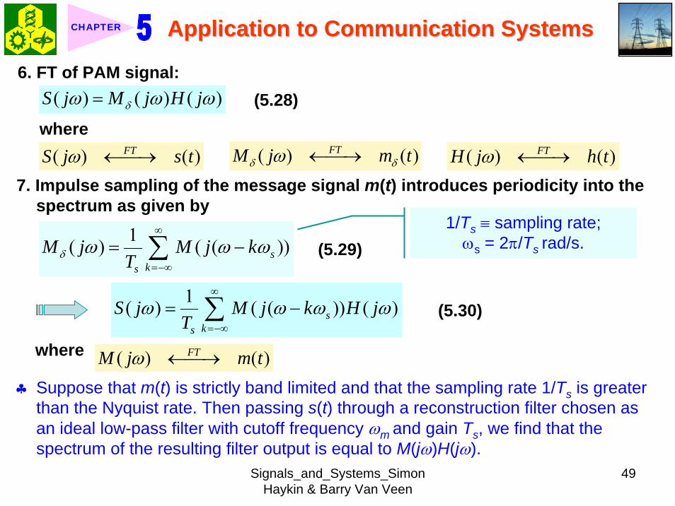
Signals_and_Systems_Simon Haykin amp Barry Van Veen
49
Application to Communication SystemsApplication to Communication SystemsCHAPTER
6 FT of PAM signal( ) ( ) ( )S j M j H jδω ω ω= (528)
where( ) ( )FTS j s tω larr⎯rarr ( ) ( )FTM j m tδ δω larr⎯rarr ( ) ( )FTH j h tω larr⎯rarr
7 Impulse sampling of the message signal m(t) introduces periodicity into the spectrum as given by
1( ) ( ( ))sks
M j M j kTδ ω ω ω
infin
=minusinfin
= minussum (529) 1Ts equiv sampling rate ωs = 2πTs rads
1( ) ( ( )) ( )sks
S j M j k H jT
ω ω ω ωinfin
=minusinfin
= minussum (530)
( ) ( )FTM j m tω larr⎯rarrwhere
clubs Suppose that m(t) is strictly band limited and that the sampling rate 1Ts is greater than the Nyquist rate Then passing s(t) through a reconstruction filter chosen as an ideal low-pass filter with cutoff frequency ωm and gain Ts we find that the spectrum of the resulting filter output is equal to M(jω)H(jω)
Signals_and_Systems_Simon Haykin amp Barry Van Veen
50
Application to Communication SystemsApplication to Communication SystemsCHAPTER
8 From Eq (525) we find that0 2
0 0( ) sin ( (2 )) j TH j T c T e ωω ω π minus= (531) Fig 524(b) magnitude and phase of H(jω)
clubs Using PAM to represent a continuous-time message signal we introduce amplitude distortion as well as a delay of T02
clubs The frequency distortion caused by the use of flat-topped sampled in the generation of a PAM wave illustrated in Fig 523Fig 523 is referred to as the aperture effect
583 583 Demodulation of PAM SignalDemodulation of PAM Signal1 Reconstruction scheme Fig 525Fig 525
Figure 525 (p 454)Figure 525 (p 454)System consisting of low-pass interpolation filter and equalizer for reconstructing a message signal from its flattopped sampled version
clubs The system consists of low-pass interpolation filter and equalizer connected in cascade
Signals_and_Systems_Simon Haykin amp Barry Van Veen
51
Application to Communication SystemsApplication to Communication SystemsCHAPTER
2 The cutoff frequency of low-pass filter = the highest frequency ωm of message signal
3 The equalizer is used to correct the aperture effect due to flat-topped sampling in the sample-and-hold circuit
4 The equalizer has the effect of decreasing the in-band loss of the interpolation filter as frequency increases in such a manner as to compensate for the aperture effect
5 Amplitude response of equalizer
0
0 0 0 0
1 1 1| ( ) | | sinc( 2) | 2 | sin( 2) |
TH j T T T T
ωω ω ω
= =
Frequency response Eq (531)
Example 55 Equalization for PAM TransmissionThe duty cycle in a PAM signal namely T0 Ts is 10 Evaluate the peak amplification required for equalizationltltSolgtSolgt1 At ωm = π Ts which corresponds to the highest frequency component of the
message signal for a sampling rate equal to the Nyquist rate we find from Eq (531) that the magnitude response of the equalizer at ωm normalized to that at zero frequency is
Signals_and_Systems_Simon Haykin amp Barry Van Veen
52
Application to Communication SystemsApplication to Communication SystemsCHAPTER
Figure 526 (p 455)Figure 526 (p 455)Normalized equalization (to compensate for aperture effect) plotted against the duty cycle T0Ts
Signals_and_Systems_Simon Haykin amp Barry Van Veen
53
Application to Communication SystemsApplication to Communication SystemsCHAPTER
0
0 0
( 2)( )1sin (05 ) sin[( 2)( )]
s
s s
T Tc T T T T
ππ
=
where the ratio T0 Ts is equal to the duty cycle of the sampling pulses 2 In Fig 526Fig 526 this result is plotted as a function of the duty cycle T0 Ts Ideally it
should be equal to unity for all values of T0 Ts 3 For a duty cycle of 10 it is equal to 10041 It follows that for duty cycles of less
than 10 the magnitude equalization required is less than 10041 in which case the aperture effect is usually considered to be negligible
59 59 Multiplexing Multiplexing clubs Three basic types of multiplexing1 Frequency-division multiplexing in which the signals are separated by
allocating them to different frequency bands This is illustrated in Fig 527(a) for the case of six different message signals Frequency-division multiplexing favors the use of CW modulation where each message signal is able to use the channel on a continuous-time basis
2 Time-division multiplexing wherein the signals are separated by allocating them to different time slots within a sampling interval
Signals_and_Systems_Simon Haykin amp Barry Van Veen
54
Application to Communication SystemsApplication to Communication SystemsCHAPTER
This second type of multiplexing is illustrated in Fig 527(b) for the case of six different message signals Code-division multiplexing which relies on the assignment of different codes to the individual users of the channel
3 Code-division multiplexing which relies on the assignment of different codes to the individual users of the channel
591 591 FrequencyFrequency--Domain Multiplexing (FDM)Domain Multiplexing (FDM)1 Block diagram Fig 528Fig 5282 Incoming message signals low-pass variety3 Low-pass filter to remove high-frequency components such that the signal
in each channel does not disturb each other4 MOD (modulator) shift the frequency ranges of the signals so as to occupy
mutually exclusive frequency intervalsSSB is often used in this stageEx Voice input is usually assigned a bandwidth of 4 kHz
5 Band-pass filters are used to restrict the band of each modulated wave to its prescribed range
6 Band-pass filters in receiver separate the message signals7 DEM (demodulator) to recover signalsclubs FDM in Fig 528 operates in only one direction
Signals_and_Systems_Simon Haykin amp Barry Van Veen
55
Application to Communication SystemsApplication to Communication SystemsCHAPTER
Figure 527 (p 456)Figure 527 (p 456)Two basic forms of multiplexing (a) Frequency-division multiplexing (with guardbands) (b) Time-division multiplexing no provision is made here for synchronizing pulses
Signals_and_Systems_Simon Haykin amp Barry Van Veen
56
Application to Communication SystemsApplication to Communication SystemsCHAPTER
Figure 528 (p 457)Figure 528 (p 457)Block diagram of FDM system showing the important constituents of the transmitter and receiver
Signals_and_Systems_Simon Haykin amp Barry Van Veen
57
Application to Communication SystemsApplication to Communication SystemsCHAPTER
Example 56 SSB-FDM System
ltltSolgtSolgt
An FDM system is used to multiplex 24 independent voice signals SSB modulation is used for the transmission Given that each voice signal is allotted a bandwidth 4kHz calculate the overall transmission bandwidth of the channel
With each voice signal allotted a bandwidth of 4 kHz the use of SSB modulation requires a bandwidth of 4 kHz for its transmission Accordingly the overall transmission bandwidth provided by the channel is 24 X 4 = 96 kHz 592 592 TimeTime--Domain Multiplexing (TDM)Domain Multiplexing (TDM)clubs Basic to the operation of a TDM system is the sampling theoremclubs The transmission of the message samples engages the transmission channel for
only a fraction of the sampling interval on a periodic basis equal to the width T0 of a PAM modulating pulse
1 Block diagram Fig 529Fig 5292 Commutator is usually implemented by means of electronic switching
circuitry3 The function of commutator is two folds
Signals_and_Systems_Simon Haykin amp Barry Van Veen
58
Application to Communication SystemsApplication to Communication SystemsCHAPTER
Figure 529 (p 458)Figure 529 (p 458)Block diagram of TDM system showing the important constituents of the transmitter and receiver
(1) To take a narrow sample of each of the M input message signals at a rate 1Tsthat is slightly higher than ωcπ where ωc is the cutoff frequency of the input low-pass filter
(2) To sequentially interleave these M samples inside a sampling interval Ts4 Pulse modulator transform the multiplexed signal into a form suitable for
transmission over the common channel
Signals_and_Systems_Simon Haykin amp Barry Van Veen
59
Application to Communication SystemsApplication to Communication SystemsCHAPTER
clubs The use of time-division multiplexing introduces a bandwidth expansion factor M because the scheme must squeeze M samples derived from M independent message sources into a time slot equal to one sampling interval
5 Pulse demodulator performs the inverse operation of the pulse modulator6 Decommutator distributes the narrow samples produced by pulse demodulator to the appropriate low-pass reconstruction filter7 Synchronization between the timing operations of the transmitter and
receiver in a TDM system is essential for satisfactory performance of the system
Inserting an extra pulse into each sampling interval on a regular basisBandwidth expansion factor is increased to M + 1
clubs The TDM system is hghly sensitive to the dispersion in the common transmission channel
Example 57 Comparison of TDM with FDMATDM system is used to multiplex four independent voice signals using PAM Each voice signal is sampled at the rate of 8 kHz The system incorporates a synchronizing pulse train for its proper operation
Signals_and_Systems_Simon Haykin amp Barry Van Veen
60
Application to Communication SystemsApplication to Communication SystemsCHAPTER
(a) Determine the timing relationships between the synchronizing pulse train and the impulse trains used to sample the four voice signals
(b) Calculate the transmission bandwidth of the channel for the TDM system and compare the result with a corresponding FDM system using SSBmodulation
ltltSolgtSolgt(a) The sampling period is
31 125 s
8 10sT s μ= =times
In this example the number of voice signals is M = 4 Hence dividing the sampling period of 125 μs among these voice signals and the synchronizing pulse train we obtain the time slot allocated to each one of them
0 1125 25 s
5
sTTM
μ
=+
= =
Signals_and_Systems_Simon Haykin amp Barry Van Veen
61
Application to Communication SystemsApplication to Communication SystemsCHAPTER
Figure 530Figure 530 shows the timing relationships between the synchronizing pulse train and the four impulse trains used to sample the different voice signals in a single frame Each frame includes time slots of common duration T0 = 25 μs which are allocated to the pulse-modulated signals and synchronizing pulse
Figure 530 (p 459)Figure 530 (p 459)Composition of one frame of a multiplexed PAM signal incorporating four voice-signals and a synchronizing pulse
Signals_and_Systems_Simon Haykin amp Barry Van Veen
62
Application to Communication SystemsApplication to Communication SystemsCHAPTER
(b) As a consequence of the time-bandwidth product (see Section 317) there is an inverse relationship between the duration of a pulse and the bandwidth (ie cutoff frequency) of the channel needed for itstransmission Accordingly the overall transmission bandwidth of the channel is
0
21 1 MHz 40 kHz
25
TTf
T
ωπ
=
= = =
In contrast the use of an FDM system based on SSB modulation requires a channel bandwidth equal to M times that of a single voice signal-that is 4 X 4 = 16 kHz Thus the use of PAM-TDM requires a channel bandwidth that is 40 16 = 25 times that of SSB-FDMIn practice pulse-code modulation is commonly used as the method of modulation for TDM this results in a further increase in channel bandwidth depending on the length of the code word used in the digital representation of each pulse in the PAM signal
Signals_and_Systems_Simon Haykin amp Barry Van Veen
63
Application to Communication SystemsApplication to Communication SystemsCHAPTER
510 510 Pulse and Group Delays Pulse and Group Delays 1 Whenever a signal is transmitted through a dispersive (ie frequency
selective) system some delay is introduced into the output signal in relation to the input signal
2 The delay is determined by the phase response of the system3 Phase response of a dispersive communication channel
( ) arg ( )H jφ ω ω= (532)
A signal is transmitted through the channel at a frequency ωc The signal received at the channel lags the transmitted signal by φ(ωc) The time delay is called phase delay formally defined as
( )cp
c
φ ωτω
= minus (533)
The phase delay is not necessarily the true signal delayclubs Case study for DSB-SC1 Transmitted signal
0( ) cos( ) cos( )cs t A t tω ω= (534)
ωc equiv carrier frequency ω0 equiv sinusoidal modulation frequency
A = AcA0
Signals_and_Systems_Simon Haykin amp Barry Van Veen
64
Application to Communication SystemsApplication to Communication SystemsCHAPTER
1 21 1( ) cos( ) cos( )2 2
s t A t A tω ω= +
1 0cω ω ω= + (535) where
2 0cω ω ω= minus (536)
Upper frequency
Lower frequency
2 Let the s(t) be transmitted through the channel with phase response φ (ω) Accordingly the signal received at the channel output is
1 1 2 21 1( ) cos( ( )) cos( ( ))2 2
y t A t A tω φ ω ω φ ω= + + +
1 2 1 20
( ) ( ) ( )1 ( )( ) cos cos2 2cy t A t tφ ω φ ω φ ω φ ωω ω+⎛ ⎞ ⎛ ⎞= + +⎜ ⎟ ⎜ ⎟
⎝ ⎠ ⎝ ⎠(537)
3 Two observations from Eq (537)1) The carrier component at frequency ωc in y(t) lags its counterpart in s(t) by
frac12 (φ (ω1) + φ (ω2)) which represents a time delay equal to
1 2 1 2
c 1 2
( )+ ( ) ( )+ ( )2 +
φ ω φ ω φ ω φ ωω ω ω
minus = minus (538)
Signals_and_Systems_Simon Haykin amp Barry Van Veen
65
Application to Communication SystemsApplication to Communication SystemsCHAPTER
2) The message component at frequency ω0 in y(t) lags its counterpart in s(t) by frac12 (φ (ω1) minus φ (ω2)) which represents a time delay equal to
1 2 1 2
0 1 2
( ) ( ) ( ) ( )2
φ ω φ ω φ ω φ ωω ω ωminus minus
minus = minusminus
(539)
4 Suppose that ω0 lt ωc rArr the side frequencies are close together with ω c between them Such a modulated signal is said to be a narrowband signal The phase response φ (ω) in the vicinity of ω = ωc is approximated by two-term Taylor series expansion
( )( ) ( ) ( )c
c cd
d ω ω
φ ωφ ω φ ω ω ωω =
= + times minus (540)
Phase delay = ( ) c cφ ω ωminus
5 The time delay introduced by the message signal (ie he ldquoenveloperdquo of the modulated signal) is given by
( )
c
gd
d ω ω
φ ωτω =
= minus (541) The time delay τg is called the
envelope delay or group delay
Signals_and_Systems_Simon Haykin amp Barry Van Veen
66
Application to Communication SystemsApplication to Communication SystemsCHAPTER
6 When a modulated signal is transmitted through a communication channel there are two different delays to be considered1) The carrier or phase delay τp defined by Eq (533)2) The envelope or group delay τg defined by Eq (541)
clubs The group delay is the true signal delay
Example 58 Phase and Group Delays for Ban-pass Channel
ltltSolgtSolgt
The phase response of a band-pass communication channel is defined by 2 2
1( ) tan c
c
ω ωφ ωωω
minus ⎛ ⎞minus= minus ⎜ ⎟
⎝ ⎠The signal s(t) defined in Eq (534) is transmitted through this channel with
475 radscω = 0 025 radsω =andCalculate (a) the phase delay and (b) the group delay
(a) At ω = ωc φ (ωc) = 0 According to Eq (533) the phase delay τ p is zero (b) Differentiating φ (ω) with respect to ω we get
Signals_and_Systems_Simon Haykin amp Barry Van Veen
67
Application to Communication SystemsApplication to Communication SystemsCHAPTER
2 2
2 2 2 2 2
( )( )( )
c c
c c
dd
ω ω ωφ ωω ω ω ω ω
+= minus
+ minus
Using thing result in Eq (541) we find that the group delay is 2 2 04211
475gc
sτω
= = =
1 One waveform shown as a solid curve was obtained by multiplying the transmitted signal s(t) by the carrier wave cos(ωct)
2 The second waveform shown as a dotted curve was obtained by multiplying the received signal y(t) by the carrier wave cos(ωct)
To display the results obtained in parts (a) and (b) in graphical form Fig 531Fig 531shows a superposition of two waveforms obtained as follows
The figure clearly shows that the carrier (phase) delay τ p is zero and the envelope of the received signal y(t) is lagging behind that of the transmitted signal by τs seconds For the presentation of waveforms in this figure we purposely did not use a filter to suppress the high frequency components resulting from the multiplications described under points 1 and 2 because of the desire to retain a contribution due to the carrier for display
Signals_and_Systems_Simon Haykin amp Barry Van Veen
68
Application to Communication SystemsApplication to Communication SystemsCHAPTER
Figure 531 Figure 531 (p 463)(p 463)Highlighting the zero carrier delay (solid curve) and group delay τg (dotted curve) which are determined in accordance with Example 58
Signals_and_Systems_Simon Haykin amp Barry Van Veen
69
Application to Communication SystemsApplication to Communication SystemsCHAPTER
clubs Not also that the separation between the upper side frequency ω1 = ωc + ω0 = 500 rads and the lower side frequency ω2 = ωc minus ω0 = 450 rads is about 10 of the carrier frequency ωc = 475 rads which justifies referring to the modulated signal in this example as a narrowband signal
5101 5101 Some Practical ConsiderationsSome Practical Considerationsclubs What is the practical importance of group delay 1 Eq (541) for determining group delay applies strictly to narrowband
modulated signal2 The message bandwidth may be comparable to the carrier frequency In
this situation the group delay is formulated as a frequency-dependent parameter ie ( )d( )g d
φ ωτ ωω
= minus (542)
3 When a wideband modulated signals transmitted through a dispersive channel the frequency components of the message signal are delayed by different amounts at the channel output
Delay distortionFig 532Fig 532 Group delay response of voice-grade telephone channel
Signals_and_Systems_Simon Haykin amp Barry Van Veen
70
Application to Communication SystemsApplication to Communication SystemsCHAPTER
Figure 532 (p 464)Group delay response of voice-grade telephone channel (Adapted from J C Bellamy Digital Telephony Wiley 1982)
511 511 Exploring Concepts with MATLABExploring Concepts with MATLAB5111 5111 Full AMFull AMclubs Sinusoidal modulation
clubs To reconstruct a faithful version of the original message signal in the receiver we have to use a delay equalizer
0( ) [1 cos( )]cos( )c cs t A t tμ ω ω= +1 AM experiment
1cA =
08 radscω π= 0 01 radsω π=Carrier amplitude
Carrier frequency Modulation amplitude
Signals_and_Systems_Simon Haykin amp Barry Van Veen
71
Application to Communication SystemsApplication to Communication SystemsCHAPTER
2 We wish to display and analyze 10 full cycles of the AM wave corresponding to a total duration of 200 s Choosing a sampling rate 1Ts = 10 Hz we have a total of N = 2000 time samples The frequency band of interest is minus 10 π ≦ ω ≦ 10 π Since the separation between the carrier and either side frequency is equal to the modulation frequency ω0 = 01 π rads we would like to have a frequency resolution ωr = 001π rads To achieve this resolution we require the following number of frequency samples (see Eq (442))
20 2000001
s
r
M ω πω π
ge = =
3 We therefore choose M = 2000 To approximate the Fourier transform of the AM wave s(t) we may use a 2000-point DTFS The only variable in the AM experiment is the modulation factor μ with respect to which we wish to investigate three different situationsμ = 05 corresponding to under-modulationμ = 10 for which the AM system is on the verge of over-modulationμ = 20 corresponding to over-modulation
Signals_and_Systems_Simon Haykin amp Barry Van Veen
72
Application to Communication SystemsApplication to Communication SystemsCHAPTER
4 MATLAB commandsAc = 1 carrier amplitudewc = 08pi carrier frequencyw0 = 01pi modulation frequencymu = 05 modulation factort = 0011999s = Ac(1 + mucos(w0t))cos(wct)plot(ts)Smag = abs(fftshift(fft(s2000)))2000 Smag denotes the magnitude specturm of the AM wavew = 10[-1000999]2pi2000plot(wSmag)axis ([-30 30 0 08])
5 5 μμ = 05 = 05 case case Fig 533Fig 533μμ = 10 case = 10 case Fig 534Fig 534μμ = 20 case = 20 case Fig 535Fig 535
Discussion see pp 466-469 textbook
Signals_and_Systems_Simon Haykin amp Barry Van Veen
73
Application to Communication SystemsApplication to Communication SystemsCHAPTER
-30 -20 -10 0 10 20 300
02
04
06
0 50 100 150 200-2
-1
0
1
2
2 22 24 26 28 3
02
04
06
(a) Time (s)
Time domain
Frequency domain
(b) Frequency (rads)
Frequency domain
Frequency (rads)
Figure 533 (p 466)Amplitude modulation with 50 modulation (a) AM wave (b) magnitude spectrum of the AM wave and (c) expanded spectrum around the carrier frequency
μμ = 05 = 05 casecase
Signals_and_Systems_Simon Haykin amp Barry Van Veen
74
Application to Communication SystemsApplication to Communication SystemsCHAPTER
Figure 534 (p 467)Figure 534 (p 467)Amplitude modulation with 100 modulation (a) AM wave (b) magnitude spectrum of the AM wave and (c) expanded spectrum around the carrier frequency
Signals_and_Systems_Simon Haykin amp Barry Van Veen
75
Application to Communication SystemsApplication to Communication SystemsCHAPTER
Figure 535 (p 468)Amplitude modulation with 200 modulation (a) AM wave (b) magnitude spectrum of the AM wave and (c) expanded spectrum around the carrier frequency
Signals_and_Systems_Simon Haykin amp Barry Van Veen
76
Application to Communication SystemsApplication to Communication SystemsCHAPTER
5112 5112 DSBDSB--SC ModulationSC Modulation1 Sinusoidal modulation
0 0( ) cos( ) cos( )c cs t A A t tω ω=
2 MATLAB commands
Ac = 1 carrier amplitudewc = 08pi carrier frequency in radsA0 = 1 amplitude of modulating signalw0 = 01pi frequency of modulating signalt = 011999s = AcA0cos(wct)cos(w0t)plot(ts)Smag = abs(fftshift(fft(s2000)))2000w = 10[-1000999]2pi2000plot(wSmag)
3 3 DSBDSB--SC modulated waveSC modulated wave Fig 536Fig 536 Discussion see pp 466-469 textbook
4 Output of the product modulator in Fig 512 (b) with φ = 0
Signals_and_Systems_Simon Haykin amp Barry Van Veen
77
Application to Communication SystemsApplication to Communication SystemsCHAPTER
Figure 536 (p 469)DSB-SC modulation (a) DSB-SC modulated wave (b) magnitude spectrum of the modulated wave and (c) expanded spectrum around the carrier frequency
Signals_and_Systems_Simon Haykin amp Barry Van Veen
78
Application to Communication SystemsApplication to Communication SystemsCHAPTER
( ) ( ) cos( )cv t s t tω=
5 MATLAB commandsgtgt v = scos(wct)
6 Fig 537 (a) waveforms of v(t) Fig 537 (b) magnitude spectrum which readily shows that v(t) consists of the following components1) A sinusoidal component with frequency 01π rads representing the
modulating wave2) A new DSB-SC modulated wave with double carrier frequency of 16π rads
in actuality the side frequencies of this modulated wave are located at 15πand 17π rads
1) The frequency of the modulating wave lies inside the passband of the filter2) The upper and lower side frequencies of the new DSB-SC modulated wave
lie inside the stopband of the filter
Accordingly we may recover the sinusoidal modulating signal by passing v(t) through low-pass filter with the following requirements
Signals_and_Systems_Simon Haykin amp Barry Van Veen
79
Application to Communication SystemsApplication to Communication SystemsCHAPTER
Figure 537 (p 470)Coherent detection of DSB-SC modulated wave (a) and (b) Waveform and magnitude spectrum of signal produced at the output of produce modulator (c) and (d) waveform and magnitude spectrum of low-pass filter output
Signals_and_Systems_Simon Haykin amp Barry Van Veen
80
Application to Communication SystemsApplication to Communication SystemsCHAPTER
The issue of how to design a filter with these requirements will be considered in detail in Chapter 8 For the present it suffices to say that the preceding requirements can be met by using the following MATLAB commands
gtgt [ba] = butter(30025)gtgt output = filter(bav)
The first command produces s special type of filter called a Butterworth filter For the experiment considered here the filter order is 3 and its normalized cutoff frequency of 0025 is calculated as follows
Actual cutoff frequency of filter 025 radsHalf the sampling rate 10 rads
0025
ππ
=
=
The second command computes the filterrsquos output in response to the product modulator output v(t) (We will revisit the design of this filter in Chapter 8) Figure 537(c) displays the waveform of the low-pass filter output this waveform represents a sinusoidal signal of frequency 005 Hz an observation that is confirmed by using the ffr command to approximate the spectrum of the filter output The result of the computation is shown in Fig 537(d)Fig 537(d)
Signals_and_Systems_Simon Haykin amp Barry Van Veen
81
Application to Communication SystemsApplication to Communication SystemsCHAPTER
7 In Fig 538 we explore another aspect of DSB-SC modulation namely the effect of varying the modulation frequency Figure 538(a) shows five cycles of a DSB-SC modulated wave that has the same carrier frequency as that in Fig 536(a) but the modulation frequency has been reduced to 0025 Hz( ie a radian frequency of 005π) Figure 538(b) shows the magnitude spectrum of this second DSB-SC modulated wave and its zoomed-in version is shown in Fig 538(c) Comparing this latter figure with Fig 536(c) we see clearly that decreasing the modulation frequency has the effect of moving the upper and lower side frequencies closer together which is consistent with modulation theory
5113 5113 Phase and Group DelayPhase and Group Delay1 In Example 58 we studied the phase and group delays for a band-pass
channel with phase response 2 2
1( ) tan c
c
ω ωφ ωωω
minus ⎛ ⎞minus= minus ⎜ ⎟
⎝ ⎠2 At ω = ωc the phase delay is τ p = 0 and the group delay is τ s = 04211s One
of the wave forms displayed in Fig 531Fig 531 is
1( ) ( ) cos( )cx t s t tω=
Signals_and_Systems_Simon Haykin amp Barry Van Veen
82
Application to Communication SystemsApplication to Communication SystemsCHAPTER
Figure 538 (p 472)Effect of varying the modulation frequency compared with that in Fig 537 (a) and (b) Waveform and magnitude spectrum of DSB-SC modulated wave with a modulation frequency one-half that used in Fig 536 (c) expanded spectrum around the carrier frequency
Signals_and_Systems_Simon Haykin amp Barry Van Veen
83
Application to Communication SystemsApplication to Communication SystemsCHAPTER
where (see page 461)
1 2( ) [cos( ) cos( )]2As t t tω ω= +
and ω1 = ωc + ω0 and ω2 = ωc - ω0 The waveform shown in the figure as a solid curve is a plot of x1(t) The other waveform also displayed in Fig 531Fig 531 is
2
1 1 2 2
( ) ( ) cos( )
[cos( ( )) cos( ( ))]cos( )2
c
c
x t y t tA t t t
ω
ω φ ω ω φ ω ω
=
= + + +
where the angle φ (ω1) and φ (ω2) are the values of the phase response φ (ω) at ω = ω1 and ω = ω2 respectively The waveform shown as a dotted curve in the figure is a plot of x2(t)
3 The generation of x1(t) and x2(t) in MATLAB is achieved with the following commands with A2 set equal to unity
Signals_and_Systems_Simon Haykin amp Barry Van Veen
84
Application to Communication SystemsApplication to Communication SystemsCHAPTER
wc = 475w0 = 025w1 = wc + w0w2 = wc - w0t = -10 0001 10o1 = -atan((w1^2 - wc^2)(w1wc))o2 = -atan((w2^2 - wc^2)(w2wc))s = cos(w1t) + cos(w2t)y = cos(w1t + o1) + cos(w2t + o2)x1 = scos(478t)x2 = ycos(475t)plot(tx1b)hold on plot(tx2k)hold offxlabel(Time)ylabel(Amplitude)
Note that we have set (A2) = 1 for convenience of presentation The function atan in the first two commands returns the arctangent Note also that the computation of both x1 and x2 involve element-by-element multiplications ndash hence the use of period followed by an asterisk
Signals_and_Systems_Simon Haykin amp Barry Van Veen
85
Application to Communication SystemsApplication to Communication SystemsCHAPTER
Signals_and_Systems_Simon Haykin amp Barry Van Veen
86
Application to Communication SystemsApplication to Communication SystemsCHAPTER
Signals_and_Systems_Simon Haykin amp Barry Van Veen
87
Application to Communication SystemsApplication to Communication SystemsCHAPTER
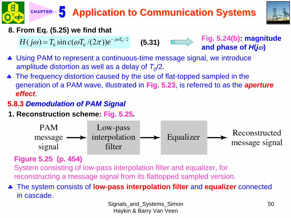
Signals_and_Systems_Simon Haykin amp Barry Van Veen
50
Application to Communication SystemsApplication to Communication SystemsCHAPTER
8 From Eq (525) we find that0 2
0 0( ) sin ( (2 )) j TH j T c T e ωω ω π minus= (531) Fig 524(b) magnitude and phase of H(jω)
clubs Using PAM to represent a continuous-time message signal we introduce amplitude distortion as well as a delay of T02
clubs The frequency distortion caused by the use of flat-topped sampled in the generation of a PAM wave illustrated in Fig 523Fig 523 is referred to as the aperture effect
583 583 Demodulation of PAM SignalDemodulation of PAM Signal1 Reconstruction scheme Fig 525Fig 525
Figure 525 (p 454)Figure 525 (p 454)System consisting of low-pass interpolation filter and equalizer for reconstructing a message signal from its flattopped sampled version
clubs The system consists of low-pass interpolation filter and equalizer connected in cascade
Signals_and_Systems_Simon Haykin amp Barry Van Veen
51
Application to Communication SystemsApplication to Communication SystemsCHAPTER
2 The cutoff frequency of low-pass filter = the highest frequency ωm of message signal
3 The equalizer is used to correct the aperture effect due to flat-topped sampling in the sample-and-hold circuit
4 The equalizer has the effect of decreasing the in-band loss of the interpolation filter as frequency increases in such a manner as to compensate for the aperture effect
5 Amplitude response of equalizer
0
0 0 0 0
1 1 1| ( ) | | sinc( 2) | 2 | sin( 2) |
TH j T T T T
ωω ω ω
= =
Frequency response Eq (531)
Example 55 Equalization for PAM TransmissionThe duty cycle in a PAM signal namely T0 Ts is 10 Evaluate the peak amplification required for equalizationltltSolgtSolgt1 At ωm = π Ts which corresponds to the highest frequency component of the
message signal for a sampling rate equal to the Nyquist rate we find from Eq (531) that the magnitude response of the equalizer at ωm normalized to that at zero frequency is
Signals_and_Systems_Simon Haykin amp Barry Van Veen
52
Application to Communication SystemsApplication to Communication SystemsCHAPTER
Figure 526 (p 455)Figure 526 (p 455)Normalized equalization (to compensate for aperture effect) plotted against the duty cycle T0Ts
Signals_and_Systems_Simon Haykin amp Barry Van Veen
53
Application to Communication SystemsApplication to Communication SystemsCHAPTER
0
0 0
( 2)( )1sin (05 ) sin[( 2)( )]
s
s s
T Tc T T T T
ππ
=
where the ratio T0 Ts is equal to the duty cycle of the sampling pulses 2 In Fig 526Fig 526 this result is plotted as a function of the duty cycle T0 Ts Ideally it
should be equal to unity for all values of T0 Ts 3 For a duty cycle of 10 it is equal to 10041 It follows that for duty cycles of less
than 10 the magnitude equalization required is less than 10041 in which case the aperture effect is usually considered to be negligible
59 59 Multiplexing Multiplexing clubs Three basic types of multiplexing1 Frequency-division multiplexing in which the signals are separated by
allocating them to different frequency bands This is illustrated in Fig 527(a) for the case of six different message signals Frequency-division multiplexing favors the use of CW modulation where each message signal is able to use the channel on a continuous-time basis
2 Time-division multiplexing wherein the signals are separated by allocating them to different time slots within a sampling interval
Signals_and_Systems_Simon Haykin amp Barry Van Veen
54
Application to Communication SystemsApplication to Communication SystemsCHAPTER
This second type of multiplexing is illustrated in Fig 527(b) for the case of six different message signals Code-division multiplexing which relies on the assignment of different codes to the individual users of the channel
3 Code-division multiplexing which relies on the assignment of different codes to the individual users of the channel
591 591 FrequencyFrequency--Domain Multiplexing (FDM)Domain Multiplexing (FDM)1 Block diagram Fig 528Fig 5282 Incoming message signals low-pass variety3 Low-pass filter to remove high-frequency components such that the signal
in each channel does not disturb each other4 MOD (modulator) shift the frequency ranges of the signals so as to occupy
mutually exclusive frequency intervalsSSB is often used in this stageEx Voice input is usually assigned a bandwidth of 4 kHz
5 Band-pass filters are used to restrict the band of each modulated wave to its prescribed range
6 Band-pass filters in receiver separate the message signals7 DEM (demodulator) to recover signalsclubs FDM in Fig 528 operates in only one direction
Signals_and_Systems_Simon Haykin amp Barry Van Veen
55
Application to Communication SystemsApplication to Communication SystemsCHAPTER
Figure 527 (p 456)Figure 527 (p 456)Two basic forms of multiplexing (a) Frequency-division multiplexing (with guardbands) (b) Time-division multiplexing no provision is made here for synchronizing pulses
Signals_and_Systems_Simon Haykin amp Barry Van Veen
56
Application to Communication SystemsApplication to Communication SystemsCHAPTER
Figure 528 (p 457)Figure 528 (p 457)Block diagram of FDM system showing the important constituents of the transmitter and receiver
Signals_and_Systems_Simon Haykin amp Barry Van Veen
57
Application to Communication SystemsApplication to Communication SystemsCHAPTER
Example 56 SSB-FDM System
ltltSolgtSolgt
An FDM system is used to multiplex 24 independent voice signals SSB modulation is used for the transmission Given that each voice signal is allotted a bandwidth 4kHz calculate the overall transmission bandwidth of the channel
With each voice signal allotted a bandwidth of 4 kHz the use of SSB modulation requires a bandwidth of 4 kHz for its transmission Accordingly the overall transmission bandwidth provided by the channel is 24 X 4 = 96 kHz 592 592 TimeTime--Domain Multiplexing (TDM)Domain Multiplexing (TDM)clubs Basic to the operation of a TDM system is the sampling theoremclubs The transmission of the message samples engages the transmission channel for
only a fraction of the sampling interval on a periodic basis equal to the width T0 of a PAM modulating pulse
1 Block diagram Fig 529Fig 5292 Commutator is usually implemented by means of electronic switching
circuitry3 The function of commutator is two folds
Signals_and_Systems_Simon Haykin amp Barry Van Veen
58
Application to Communication SystemsApplication to Communication SystemsCHAPTER
Figure 529 (p 458)Figure 529 (p 458)Block diagram of TDM system showing the important constituents of the transmitter and receiver
(1) To take a narrow sample of each of the M input message signals at a rate 1Tsthat is slightly higher than ωcπ where ωc is the cutoff frequency of the input low-pass filter
(2) To sequentially interleave these M samples inside a sampling interval Ts4 Pulse modulator transform the multiplexed signal into a form suitable for
transmission over the common channel
Signals_and_Systems_Simon Haykin amp Barry Van Veen
59
Application to Communication SystemsApplication to Communication SystemsCHAPTER
clubs The use of time-division multiplexing introduces a bandwidth expansion factor M because the scheme must squeeze M samples derived from M independent message sources into a time slot equal to one sampling interval
5 Pulse demodulator performs the inverse operation of the pulse modulator6 Decommutator distributes the narrow samples produced by pulse demodulator to the appropriate low-pass reconstruction filter7 Synchronization between the timing operations of the transmitter and
receiver in a TDM system is essential for satisfactory performance of the system
Inserting an extra pulse into each sampling interval on a regular basisBandwidth expansion factor is increased to M + 1
clubs The TDM system is hghly sensitive to the dispersion in the common transmission channel
Example 57 Comparison of TDM with FDMATDM system is used to multiplex four independent voice signals using PAM Each voice signal is sampled at the rate of 8 kHz The system incorporates a synchronizing pulse train for its proper operation
Signals_and_Systems_Simon Haykin amp Barry Van Veen
60
Application to Communication SystemsApplication to Communication SystemsCHAPTER
(a) Determine the timing relationships between the synchronizing pulse train and the impulse trains used to sample the four voice signals
(b) Calculate the transmission bandwidth of the channel for the TDM system and compare the result with a corresponding FDM system using SSBmodulation
ltltSolgtSolgt(a) The sampling period is
31 125 s
8 10sT s μ= =times
In this example the number of voice signals is M = 4 Hence dividing the sampling period of 125 μs among these voice signals and the synchronizing pulse train we obtain the time slot allocated to each one of them
0 1125 25 s
5
sTTM
μ
=+
= =
Signals_and_Systems_Simon Haykin amp Barry Van Veen
61
Application to Communication SystemsApplication to Communication SystemsCHAPTER
Figure 530Figure 530 shows the timing relationships between the synchronizing pulse train and the four impulse trains used to sample the different voice signals in a single frame Each frame includes time slots of common duration T0 = 25 μs which are allocated to the pulse-modulated signals and synchronizing pulse
Figure 530 (p 459)Figure 530 (p 459)Composition of one frame of a multiplexed PAM signal incorporating four voice-signals and a synchronizing pulse
Signals_and_Systems_Simon Haykin amp Barry Van Veen
62
Application to Communication SystemsApplication to Communication SystemsCHAPTER
(b) As a consequence of the time-bandwidth product (see Section 317) there is an inverse relationship between the duration of a pulse and the bandwidth (ie cutoff frequency) of the channel needed for itstransmission Accordingly the overall transmission bandwidth of the channel is
0
21 1 MHz 40 kHz
25
TTf
T
ωπ
=
= = =
In contrast the use of an FDM system based on SSB modulation requires a channel bandwidth equal to M times that of a single voice signal-that is 4 X 4 = 16 kHz Thus the use of PAM-TDM requires a channel bandwidth that is 40 16 = 25 times that of SSB-FDMIn practice pulse-code modulation is commonly used as the method of modulation for TDM this results in a further increase in channel bandwidth depending on the length of the code word used in the digital representation of each pulse in the PAM signal
Signals_and_Systems_Simon Haykin amp Barry Van Veen
63
Application to Communication SystemsApplication to Communication SystemsCHAPTER
510 510 Pulse and Group Delays Pulse and Group Delays 1 Whenever a signal is transmitted through a dispersive (ie frequency
selective) system some delay is introduced into the output signal in relation to the input signal
2 The delay is determined by the phase response of the system3 Phase response of a dispersive communication channel
( ) arg ( )H jφ ω ω= (532)
A signal is transmitted through the channel at a frequency ωc The signal received at the channel lags the transmitted signal by φ(ωc) The time delay is called phase delay formally defined as
( )cp
c
φ ωτω
= minus (533)
The phase delay is not necessarily the true signal delayclubs Case study for DSB-SC1 Transmitted signal
0( ) cos( ) cos( )cs t A t tω ω= (534)
ωc equiv carrier frequency ω0 equiv sinusoidal modulation frequency
A = AcA0
Signals_and_Systems_Simon Haykin amp Barry Van Veen
64
Application to Communication SystemsApplication to Communication SystemsCHAPTER
1 21 1( ) cos( ) cos( )2 2
s t A t A tω ω= +
1 0cω ω ω= + (535) where
2 0cω ω ω= minus (536)
Upper frequency
Lower frequency
2 Let the s(t) be transmitted through the channel with phase response φ (ω) Accordingly the signal received at the channel output is
1 1 2 21 1( ) cos( ( )) cos( ( ))2 2
y t A t A tω φ ω ω φ ω= + + +
1 2 1 20
( ) ( ) ( )1 ( )( ) cos cos2 2cy t A t tφ ω φ ω φ ω φ ωω ω+⎛ ⎞ ⎛ ⎞= + +⎜ ⎟ ⎜ ⎟
⎝ ⎠ ⎝ ⎠(537)
3 Two observations from Eq (537)1) The carrier component at frequency ωc in y(t) lags its counterpart in s(t) by
frac12 (φ (ω1) + φ (ω2)) which represents a time delay equal to
1 2 1 2
c 1 2
( )+ ( ) ( )+ ( )2 +
φ ω φ ω φ ω φ ωω ω ω
minus = minus (538)
Signals_and_Systems_Simon Haykin amp Barry Van Veen
65
Application to Communication SystemsApplication to Communication SystemsCHAPTER
2) The message component at frequency ω0 in y(t) lags its counterpart in s(t) by frac12 (φ (ω1) minus φ (ω2)) which represents a time delay equal to
1 2 1 2
0 1 2
( ) ( ) ( ) ( )2
φ ω φ ω φ ω φ ωω ω ωminus minus
minus = minusminus
(539)
4 Suppose that ω0 lt ωc rArr the side frequencies are close together with ω c between them Such a modulated signal is said to be a narrowband signal The phase response φ (ω) in the vicinity of ω = ωc is approximated by two-term Taylor series expansion
( )( ) ( ) ( )c
c cd
d ω ω
φ ωφ ω φ ω ω ωω =
= + times minus (540)
Phase delay = ( ) c cφ ω ωminus
5 The time delay introduced by the message signal (ie he ldquoenveloperdquo of the modulated signal) is given by
( )
c
gd
d ω ω
φ ωτω =
= minus (541) The time delay τg is called the
envelope delay or group delay
Signals_and_Systems_Simon Haykin amp Barry Van Veen
66
Application to Communication SystemsApplication to Communication SystemsCHAPTER
6 When a modulated signal is transmitted through a communication channel there are two different delays to be considered1) The carrier or phase delay τp defined by Eq (533)2) The envelope or group delay τg defined by Eq (541)
clubs The group delay is the true signal delay
Example 58 Phase and Group Delays for Ban-pass Channel
ltltSolgtSolgt
The phase response of a band-pass communication channel is defined by 2 2
1( ) tan c
c
ω ωφ ωωω
minus ⎛ ⎞minus= minus ⎜ ⎟
⎝ ⎠The signal s(t) defined in Eq (534) is transmitted through this channel with
475 radscω = 0 025 radsω =andCalculate (a) the phase delay and (b) the group delay
(a) At ω = ωc φ (ωc) = 0 According to Eq (533) the phase delay τ p is zero (b) Differentiating φ (ω) with respect to ω we get
Signals_and_Systems_Simon Haykin amp Barry Van Veen
67
Application to Communication SystemsApplication to Communication SystemsCHAPTER
2 2
2 2 2 2 2
( )( )( )
c c
c c
dd
ω ω ωφ ωω ω ω ω ω
+= minus
+ minus
Using thing result in Eq (541) we find that the group delay is 2 2 04211
475gc
sτω
= = =
1 One waveform shown as a solid curve was obtained by multiplying the transmitted signal s(t) by the carrier wave cos(ωct)
2 The second waveform shown as a dotted curve was obtained by multiplying the received signal y(t) by the carrier wave cos(ωct)
To display the results obtained in parts (a) and (b) in graphical form Fig 531Fig 531shows a superposition of two waveforms obtained as follows
The figure clearly shows that the carrier (phase) delay τ p is zero and the envelope of the received signal y(t) is lagging behind that of the transmitted signal by τs seconds For the presentation of waveforms in this figure we purposely did not use a filter to suppress the high frequency components resulting from the multiplications described under points 1 and 2 because of the desire to retain a contribution due to the carrier for display
Signals_and_Systems_Simon Haykin amp Barry Van Veen
68
Application to Communication SystemsApplication to Communication SystemsCHAPTER
Figure 531 Figure 531 (p 463)(p 463)Highlighting the zero carrier delay (solid curve) and group delay τg (dotted curve) which are determined in accordance with Example 58
Signals_and_Systems_Simon Haykin amp Barry Van Veen
69
Application to Communication SystemsApplication to Communication SystemsCHAPTER
clubs Not also that the separation between the upper side frequency ω1 = ωc + ω0 = 500 rads and the lower side frequency ω2 = ωc minus ω0 = 450 rads is about 10 of the carrier frequency ωc = 475 rads which justifies referring to the modulated signal in this example as a narrowband signal
5101 5101 Some Practical ConsiderationsSome Practical Considerationsclubs What is the practical importance of group delay 1 Eq (541) for determining group delay applies strictly to narrowband
modulated signal2 The message bandwidth may be comparable to the carrier frequency In
this situation the group delay is formulated as a frequency-dependent parameter ie ( )d( )g d
φ ωτ ωω
= minus (542)
3 When a wideband modulated signals transmitted through a dispersive channel the frequency components of the message signal are delayed by different amounts at the channel output
Delay distortionFig 532Fig 532 Group delay response of voice-grade telephone channel
Signals_and_Systems_Simon Haykin amp Barry Van Veen
70
Application to Communication SystemsApplication to Communication SystemsCHAPTER
Figure 532 (p 464)Group delay response of voice-grade telephone channel (Adapted from J C Bellamy Digital Telephony Wiley 1982)
511 511 Exploring Concepts with MATLABExploring Concepts with MATLAB5111 5111 Full AMFull AMclubs Sinusoidal modulation
clubs To reconstruct a faithful version of the original message signal in the receiver we have to use a delay equalizer
0( ) [1 cos( )]cos( )c cs t A t tμ ω ω= +1 AM experiment
1cA =
08 radscω π= 0 01 radsω π=Carrier amplitude
Carrier frequency Modulation amplitude
Signals_and_Systems_Simon Haykin amp Barry Van Veen
71
Application to Communication SystemsApplication to Communication SystemsCHAPTER
2 We wish to display and analyze 10 full cycles of the AM wave corresponding to a total duration of 200 s Choosing a sampling rate 1Ts = 10 Hz we have a total of N = 2000 time samples The frequency band of interest is minus 10 π ≦ ω ≦ 10 π Since the separation between the carrier and either side frequency is equal to the modulation frequency ω0 = 01 π rads we would like to have a frequency resolution ωr = 001π rads To achieve this resolution we require the following number of frequency samples (see Eq (442))
20 2000001
s
r
M ω πω π
ge = =
3 We therefore choose M = 2000 To approximate the Fourier transform of the AM wave s(t) we may use a 2000-point DTFS The only variable in the AM experiment is the modulation factor μ with respect to which we wish to investigate three different situationsμ = 05 corresponding to under-modulationμ = 10 for which the AM system is on the verge of over-modulationμ = 20 corresponding to over-modulation
Signals_and_Systems_Simon Haykin amp Barry Van Veen
72
Application to Communication SystemsApplication to Communication SystemsCHAPTER
4 MATLAB commandsAc = 1 carrier amplitudewc = 08pi carrier frequencyw0 = 01pi modulation frequencymu = 05 modulation factort = 0011999s = Ac(1 + mucos(w0t))cos(wct)plot(ts)Smag = abs(fftshift(fft(s2000)))2000 Smag denotes the magnitude specturm of the AM wavew = 10[-1000999]2pi2000plot(wSmag)axis ([-30 30 0 08])
5 5 μμ = 05 = 05 case case Fig 533Fig 533μμ = 10 case = 10 case Fig 534Fig 534μμ = 20 case = 20 case Fig 535Fig 535
Discussion see pp 466-469 textbook
Signals_and_Systems_Simon Haykin amp Barry Van Veen
73
Application to Communication SystemsApplication to Communication SystemsCHAPTER
-30 -20 -10 0 10 20 300
02
04
06
0 50 100 150 200-2
-1
0
1
2
2 22 24 26 28 3
02
04
06
(a) Time (s)
Time domain
Frequency domain
(b) Frequency (rads)
Frequency domain
Frequency (rads)
Figure 533 (p 466)Amplitude modulation with 50 modulation (a) AM wave (b) magnitude spectrum of the AM wave and (c) expanded spectrum around the carrier frequency
μμ = 05 = 05 casecase
Signals_and_Systems_Simon Haykin amp Barry Van Veen
74
Application to Communication SystemsApplication to Communication SystemsCHAPTER
Figure 534 (p 467)Figure 534 (p 467)Amplitude modulation with 100 modulation (a) AM wave (b) magnitude spectrum of the AM wave and (c) expanded spectrum around the carrier frequency
Signals_and_Systems_Simon Haykin amp Barry Van Veen
75
Application to Communication SystemsApplication to Communication SystemsCHAPTER
Figure 535 (p 468)Amplitude modulation with 200 modulation (a) AM wave (b) magnitude spectrum of the AM wave and (c) expanded spectrum around the carrier frequency
Signals_and_Systems_Simon Haykin amp Barry Van Veen
76
Application to Communication SystemsApplication to Communication SystemsCHAPTER
5112 5112 DSBDSB--SC ModulationSC Modulation1 Sinusoidal modulation
0 0( ) cos( ) cos( )c cs t A A t tω ω=
2 MATLAB commands
Ac = 1 carrier amplitudewc = 08pi carrier frequency in radsA0 = 1 amplitude of modulating signalw0 = 01pi frequency of modulating signalt = 011999s = AcA0cos(wct)cos(w0t)plot(ts)Smag = abs(fftshift(fft(s2000)))2000w = 10[-1000999]2pi2000plot(wSmag)
3 3 DSBDSB--SC modulated waveSC modulated wave Fig 536Fig 536 Discussion see pp 466-469 textbook
4 Output of the product modulator in Fig 512 (b) with φ = 0
Signals_and_Systems_Simon Haykin amp Barry Van Veen
77
Application to Communication SystemsApplication to Communication SystemsCHAPTER
Figure 536 (p 469)DSB-SC modulation (a) DSB-SC modulated wave (b) magnitude spectrum of the modulated wave and (c) expanded spectrum around the carrier frequency
Signals_and_Systems_Simon Haykin amp Barry Van Veen
78
Application to Communication SystemsApplication to Communication SystemsCHAPTER
( ) ( ) cos( )cv t s t tω=
5 MATLAB commandsgtgt v = scos(wct)
6 Fig 537 (a) waveforms of v(t) Fig 537 (b) magnitude spectrum which readily shows that v(t) consists of the following components1) A sinusoidal component with frequency 01π rads representing the
modulating wave2) A new DSB-SC modulated wave with double carrier frequency of 16π rads
in actuality the side frequencies of this modulated wave are located at 15πand 17π rads
1) The frequency of the modulating wave lies inside the passband of the filter2) The upper and lower side frequencies of the new DSB-SC modulated wave
lie inside the stopband of the filter
Accordingly we may recover the sinusoidal modulating signal by passing v(t) through low-pass filter with the following requirements
Signals_and_Systems_Simon Haykin amp Barry Van Veen
79
Application to Communication SystemsApplication to Communication SystemsCHAPTER
Figure 537 (p 470)Coherent detection of DSB-SC modulated wave (a) and (b) Waveform and magnitude spectrum of signal produced at the output of produce modulator (c) and (d) waveform and magnitude spectrum of low-pass filter output
Signals_and_Systems_Simon Haykin amp Barry Van Veen
80
Application to Communication SystemsApplication to Communication SystemsCHAPTER
The issue of how to design a filter with these requirements will be considered in detail in Chapter 8 For the present it suffices to say that the preceding requirements can be met by using the following MATLAB commands
gtgt [ba] = butter(30025)gtgt output = filter(bav)
The first command produces s special type of filter called a Butterworth filter For the experiment considered here the filter order is 3 and its normalized cutoff frequency of 0025 is calculated as follows
Actual cutoff frequency of filter 025 radsHalf the sampling rate 10 rads
0025
ππ
=
=
The second command computes the filterrsquos output in response to the product modulator output v(t) (We will revisit the design of this filter in Chapter 8) Figure 537(c) displays the waveform of the low-pass filter output this waveform represents a sinusoidal signal of frequency 005 Hz an observation that is confirmed by using the ffr command to approximate the spectrum of the filter output The result of the computation is shown in Fig 537(d)Fig 537(d)
Signals_and_Systems_Simon Haykin amp Barry Van Veen
81
Application to Communication SystemsApplication to Communication SystemsCHAPTER
7 In Fig 538 we explore another aspect of DSB-SC modulation namely the effect of varying the modulation frequency Figure 538(a) shows five cycles of a DSB-SC modulated wave that has the same carrier frequency as that in Fig 536(a) but the modulation frequency has been reduced to 0025 Hz( ie a radian frequency of 005π) Figure 538(b) shows the magnitude spectrum of this second DSB-SC modulated wave and its zoomed-in version is shown in Fig 538(c) Comparing this latter figure with Fig 536(c) we see clearly that decreasing the modulation frequency has the effect of moving the upper and lower side frequencies closer together which is consistent with modulation theory
5113 5113 Phase and Group DelayPhase and Group Delay1 In Example 58 we studied the phase and group delays for a band-pass
channel with phase response 2 2
1( ) tan c
c
ω ωφ ωωω
minus ⎛ ⎞minus= minus ⎜ ⎟
⎝ ⎠2 At ω = ωc the phase delay is τ p = 0 and the group delay is τ s = 04211s One
of the wave forms displayed in Fig 531Fig 531 is
1( ) ( ) cos( )cx t s t tω=
Signals_and_Systems_Simon Haykin amp Barry Van Veen
82
Application to Communication SystemsApplication to Communication SystemsCHAPTER
Figure 538 (p 472)Effect of varying the modulation frequency compared with that in Fig 537 (a) and (b) Waveform and magnitude spectrum of DSB-SC modulated wave with a modulation frequency one-half that used in Fig 536 (c) expanded spectrum around the carrier frequency
Signals_and_Systems_Simon Haykin amp Barry Van Veen
83
Application to Communication SystemsApplication to Communication SystemsCHAPTER
where (see page 461)
1 2( ) [cos( ) cos( )]2As t t tω ω= +
and ω1 = ωc + ω0 and ω2 = ωc - ω0 The waveform shown in the figure as a solid curve is a plot of x1(t) The other waveform also displayed in Fig 531Fig 531 is
2
1 1 2 2
( ) ( ) cos( )
[cos( ( )) cos( ( ))]cos( )2
c
c
x t y t tA t t t
ω
ω φ ω ω φ ω ω
=
= + + +
where the angle φ (ω1) and φ (ω2) are the values of the phase response φ (ω) at ω = ω1 and ω = ω2 respectively The waveform shown as a dotted curve in the figure is a plot of x2(t)
3 The generation of x1(t) and x2(t) in MATLAB is achieved with the following commands with A2 set equal to unity
Signals_and_Systems_Simon Haykin amp Barry Van Veen
84
Application to Communication SystemsApplication to Communication SystemsCHAPTER
wc = 475w0 = 025w1 = wc + w0w2 = wc - w0t = -10 0001 10o1 = -atan((w1^2 - wc^2)(w1wc))o2 = -atan((w2^2 - wc^2)(w2wc))s = cos(w1t) + cos(w2t)y = cos(w1t + o1) + cos(w2t + o2)x1 = scos(478t)x2 = ycos(475t)plot(tx1b)hold on plot(tx2k)hold offxlabel(Time)ylabel(Amplitude)
Note that we have set (A2) = 1 for convenience of presentation The function atan in the first two commands returns the arctangent Note also that the computation of both x1 and x2 involve element-by-element multiplications ndash hence the use of period followed by an asterisk
Signals_and_Systems_Simon Haykin amp Barry Van Veen
85
Application to Communication SystemsApplication to Communication SystemsCHAPTER
Signals_and_Systems_Simon Haykin amp Barry Van Veen
86
Application to Communication SystemsApplication to Communication SystemsCHAPTER
Signals_and_Systems_Simon Haykin amp Barry Van Veen
87
Application to Communication SystemsApplication to Communication SystemsCHAPTER
Signals_and_Systems_Simon Haykin amp Barry Van Veen
51
Application to Communication SystemsApplication to Communication SystemsCHAPTER
2 The cutoff frequency of low-pass filter = the highest frequency ωm of message signal
3 The equalizer is used to correct the aperture effect due to flat-topped sampling in the sample-and-hold circuit
4 The equalizer has the effect of decreasing the in-band loss of the interpolation filter as frequency increases in such a manner as to compensate for the aperture effect
5 Amplitude response of equalizer
0
0 0 0 0
1 1 1| ( ) | | sinc( 2) | 2 | sin( 2) |
TH j T T T T
ωω ω ω
= =
Frequency response Eq (531)
Example 55 Equalization for PAM TransmissionThe duty cycle in a PAM signal namely T0 Ts is 10 Evaluate the peak amplification required for equalizationltltSolgtSolgt1 At ωm = π Ts which corresponds to the highest frequency component of the
message signal for a sampling rate equal to the Nyquist rate we find from Eq (531) that the magnitude response of the equalizer at ωm normalized to that at zero frequency is
Signals_and_Systems_Simon Haykin amp Barry Van Veen
52
Application to Communication SystemsApplication to Communication SystemsCHAPTER
Figure 526 (p 455)Figure 526 (p 455)Normalized equalization (to compensate for aperture effect) plotted against the duty cycle T0Ts
Signals_and_Systems_Simon Haykin amp Barry Van Veen
53
Application to Communication SystemsApplication to Communication SystemsCHAPTER
0
0 0
( 2)( )1sin (05 ) sin[( 2)( )]
s
s s
T Tc T T T T
ππ
=
where the ratio T0 Ts is equal to the duty cycle of the sampling pulses 2 In Fig 526Fig 526 this result is plotted as a function of the duty cycle T0 Ts Ideally it
should be equal to unity for all values of T0 Ts 3 For a duty cycle of 10 it is equal to 10041 It follows that for duty cycles of less
than 10 the magnitude equalization required is less than 10041 in which case the aperture effect is usually considered to be negligible
59 59 Multiplexing Multiplexing clubs Three basic types of multiplexing1 Frequency-division multiplexing in which the signals are separated by
allocating them to different frequency bands This is illustrated in Fig 527(a) for the case of six different message signals Frequency-division multiplexing favors the use of CW modulation where each message signal is able to use the channel on a continuous-time basis
2 Time-division multiplexing wherein the signals are separated by allocating them to different time slots within a sampling interval
Signals_and_Systems_Simon Haykin amp Barry Van Veen
54
Application to Communication SystemsApplication to Communication SystemsCHAPTER
This second type of multiplexing is illustrated in Fig 527(b) for the case of six different message signals Code-division multiplexing which relies on the assignment of different codes to the individual users of the channel
3 Code-division multiplexing which relies on the assignment of different codes to the individual users of the channel
591 591 FrequencyFrequency--Domain Multiplexing (FDM)Domain Multiplexing (FDM)1 Block diagram Fig 528Fig 5282 Incoming message signals low-pass variety3 Low-pass filter to remove high-frequency components such that the signal
in each channel does not disturb each other4 MOD (modulator) shift the frequency ranges of the signals so as to occupy
mutually exclusive frequency intervalsSSB is often used in this stageEx Voice input is usually assigned a bandwidth of 4 kHz
5 Band-pass filters are used to restrict the band of each modulated wave to its prescribed range
6 Band-pass filters in receiver separate the message signals7 DEM (demodulator) to recover signalsclubs FDM in Fig 528 operates in only one direction
Signals_and_Systems_Simon Haykin amp Barry Van Veen
55
Application to Communication SystemsApplication to Communication SystemsCHAPTER
Figure 527 (p 456)Figure 527 (p 456)Two basic forms of multiplexing (a) Frequency-division multiplexing (with guardbands) (b) Time-division multiplexing no provision is made here for synchronizing pulses
Signals_and_Systems_Simon Haykin amp Barry Van Veen
56
Application to Communication SystemsApplication to Communication SystemsCHAPTER
Figure 528 (p 457)Figure 528 (p 457)Block diagram of FDM system showing the important constituents of the transmitter and receiver
Signals_and_Systems_Simon Haykin amp Barry Van Veen
57
Application to Communication SystemsApplication to Communication SystemsCHAPTER
Example 56 SSB-FDM System
ltltSolgtSolgt
An FDM system is used to multiplex 24 independent voice signals SSB modulation is used for the transmission Given that each voice signal is allotted a bandwidth 4kHz calculate the overall transmission bandwidth of the channel
With each voice signal allotted a bandwidth of 4 kHz the use of SSB modulation requires a bandwidth of 4 kHz for its transmission Accordingly the overall transmission bandwidth provided by the channel is 24 X 4 = 96 kHz 592 592 TimeTime--Domain Multiplexing (TDM)Domain Multiplexing (TDM)clubs Basic to the operation of a TDM system is the sampling theoremclubs The transmission of the message samples engages the transmission channel for
only a fraction of the sampling interval on a periodic basis equal to the width T0 of a PAM modulating pulse
1 Block diagram Fig 529Fig 5292 Commutator is usually implemented by means of electronic switching
circuitry3 The function of commutator is two folds
Signals_and_Systems_Simon Haykin amp Barry Van Veen
58
Application to Communication SystemsApplication to Communication SystemsCHAPTER
Figure 529 (p 458)Figure 529 (p 458)Block diagram of TDM system showing the important constituents of the transmitter and receiver
(1) To take a narrow sample of each of the M input message signals at a rate 1Tsthat is slightly higher than ωcπ where ωc is the cutoff frequency of the input low-pass filter
(2) To sequentially interleave these M samples inside a sampling interval Ts4 Pulse modulator transform the multiplexed signal into a form suitable for
transmission over the common channel
Signals_and_Systems_Simon Haykin amp Barry Van Veen
59
Application to Communication SystemsApplication to Communication SystemsCHAPTER
clubs The use of time-division multiplexing introduces a bandwidth expansion factor M because the scheme must squeeze M samples derived from M independent message sources into a time slot equal to one sampling interval
5 Pulse demodulator performs the inverse operation of the pulse modulator6 Decommutator distributes the narrow samples produced by pulse demodulator to the appropriate low-pass reconstruction filter7 Synchronization between the timing operations of the transmitter and
receiver in a TDM system is essential for satisfactory performance of the system
Inserting an extra pulse into each sampling interval on a regular basisBandwidth expansion factor is increased to M + 1
clubs The TDM system is hghly sensitive to the dispersion in the common transmission channel
Example 57 Comparison of TDM with FDMATDM system is used to multiplex four independent voice signals using PAM Each voice signal is sampled at the rate of 8 kHz The system incorporates a synchronizing pulse train for its proper operation
Signals_and_Systems_Simon Haykin amp Barry Van Veen
60
Application to Communication SystemsApplication to Communication SystemsCHAPTER
(a) Determine the timing relationships between the synchronizing pulse train and the impulse trains used to sample the four voice signals
(b) Calculate the transmission bandwidth of the channel for the TDM system and compare the result with a corresponding FDM system using SSBmodulation
ltltSolgtSolgt(a) The sampling period is
31 125 s
8 10sT s μ= =times
In this example the number of voice signals is M = 4 Hence dividing the sampling period of 125 μs among these voice signals and the synchronizing pulse train we obtain the time slot allocated to each one of them
0 1125 25 s
5
sTTM
μ
=+
= =
Signals_and_Systems_Simon Haykin amp Barry Van Veen
61
Application to Communication SystemsApplication to Communication SystemsCHAPTER
Figure 530Figure 530 shows the timing relationships between the synchronizing pulse train and the four impulse trains used to sample the different voice signals in a single frame Each frame includes time slots of common duration T0 = 25 μs which are allocated to the pulse-modulated signals and synchronizing pulse
Figure 530 (p 459)Figure 530 (p 459)Composition of one frame of a multiplexed PAM signal incorporating four voice-signals and a synchronizing pulse
Signals_and_Systems_Simon Haykin amp Barry Van Veen
62
Application to Communication SystemsApplication to Communication SystemsCHAPTER
(b) As a consequence of the time-bandwidth product (see Section 317) there is an inverse relationship between the duration of a pulse and the bandwidth (ie cutoff frequency) of the channel needed for itstransmission Accordingly the overall transmission bandwidth of the channel is
0
21 1 MHz 40 kHz
25
TTf
T
ωπ
=
= = =
In contrast the use of an FDM system based on SSB modulation requires a channel bandwidth equal to M times that of a single voice signal-that is 4 X 4 = 16 kHz Thus the use of PAM-TDM requires a channel bandwidth that is 40 16 = 25 times that of SSB-FDMIn practice pulse-code modulation is commonly used as the method of modulation for TDM this results in a further increase in channel bandwidth depending on the length of the code word used in the digital representation of each pulse in the PAM signal
Signals_and_Systems_Simon Haykin amp Barry Van Veen
63
Application to Communication SystemsApplication to Communication SystemsCHAPTER
510 510 Pulse and Group Delays Pulse and Group Delays 1 Whenever a signal is transmitted through a dispersive (ie frequency
selective) system some delay is introduced into the output signal in relation to the input signal
2 The delay is determined by the phase response of the system3 Phase response of a dispersive communication channel
( ) arg ( )H jφ ω ω= (532)
A signal is transmitted through the channel at a frequency ωc The signal received at the channel lags the transmitted signal by φ(ωc) The time delay is called phase delay formally defined as
( )cp
c
φ ωτω
= minus (533)
The phase delay is not necessarily the true signal delayclubs Case study for DSB-SC1 Transmitted signal
0( ) cos( ) cos( )cs t A t tω ω= (534)
ωc equiv carrier frequency ω0 equiv sinusoidal modulation frequency
A = AcA0
Signals_and_Systems_Simon Haykin amp Barry Van Veen
64
Application to Communication SystemsApplication to Communication SystemsCHAPTER
1 21 1( ) cos( ) cos( )2 2
s t A t A tω ω= +
1 0cω ω ω= + (535) where
2 0cω ω ω= minus (536)
Upper frequency
Lower frequency
2 Let the s(t) be transmitted through the channel with phase response φ (ω) Accordingly the signal received at the channel output is
1 1 2 21 1( ) cos( ( )) cos( ( ))2 2
y t A t A tω φ ω ω φ ω= + + +
1 2 1 20
( ) ( ) ( )1 ( )( ) cos cos2 2cy t A t tφ ω φ ω φ ω φ ωω ω+⎛ ⎞ ⎛ ⎞= + +⎜ ⎟ ⎜ ⎟
⎝ ⎠ ⎝ ⎠(537)
3 Two observations from Eq (537)1) The carrier component at frequency ωc in y(t) lags its counterpart in s(t) by
frac12 (φ (ω1) + φ (ω2)) which represents a time delay equal to
1 2 1 2
c 1 2
( )+ ( ) ( )+ ( )2 +
φ ω φ ω φ ω φ ωω ω ω
minus = minus (538)
Signals_and_Systems_Simon Haykin amp Barry Van Veen
65
Application to Communication SystemsApplication to Communication SystemsCHAPTER
2) The message component at frequency ω0 in y(t) lags its counterpart in s(t) by frac12 (φ (ω1) minus φ (ω2)) which represents a time delay equal to
1 2 1 2
0 1 2
( ) ( ) ( ) ( )2
φ ω φ ω φ ω φ ωω ω ωminus minus
minus = minusminus
(539)
4 Suppose that ω0 lt ωc rArr the side frequencies are close together with ω c between them Such a modulated signal is said to be a narrowband signal The phase response φ (ω) in the vicinity of ω = ωc is approximated by two-term Taylor series expansion
( )( ) ( ) ( )c
c cd
d ω ω
φ ωφ ω φ ω ω ωω =
= + times minus (540)
Phase delay = ( ) c cφ ω ωminus
5 The time delay introduced by the message signal (ie he ldquoenveloperdquo of the modulated signal) is given by
( )
c
gd
d ω ω
φ ωτω =
= minus (541) The time delay τg is called the
envelope delay or group delay
Signals_and_Systems_Simon Haykin amp Barry Van Veen
66
Application to Communication SystemsApplication to Communication SystemsCHAPTER
6 When a modulated signal is transmitted through a communication channel there are two different delays to be considered1) The carrier or phase delay τp defined by Eq (533)2) The envelope or group delay τg defined by Eq (541)
clubs The group delay is the true signal delay
Example 58 Phase and Group Delays for Ban-pass Channel
ltltSolgtSolgt
The phase response of a band-pass communication channel is defined by 2 2
1( ) tan c
c
ω ωφ ωωω
minus ⎛ ⎞minus= minus ⎜ ⎟
⎝ ⎠The signal s(t) defined in Eq (534) is transmitted through this channel with
475 radscω = 0 025 radsω =andCalculate (a) the phase delay and (b) the group delay
(a) At ω = ωc φ (ωc) = 0 According to Eq (533) the phase delay τ p is zero (b) Differentiating φ (ω) with respect to ω we get
Signals_and_Systems_Simon Haykin amp Barry Van Veen
67
Application to Communication SystemsApplication to Communication SystemsCHAPTER
2 2
2 2 2 2 2
( )( )( )
c c
c c
dd
ω ω ωφ ωω ω ω ω ω
+= minus
+ minus
Using thing result in Eq (541) we find that the group delay is 2 2 04211
475gc
sτω
= = =
1 One waveform shown as a solid curve was obtained by multiplying the transmitted signal s(t) by the carrier wave cos(ωct)
2 The second waveform shown as a dotted curve was obtained by multiplying the received signal y(t) by the carrier wave cos(ωct)
To display the results obtained in parts (a) and (b) in graphical form Fig 531Fig 531shows a superposition of two waveforms obtained as follows
The figure clearly shows that the carrier (phase) delay τ p is zero and the envelope of the received signal y(t) is lagging behind that of the transmitted signal by τs seconds For the presentation of waveforms in this figure we purposely did not use a filter to suppress the high frequency components resulting from the multiplications described under points 1 and 2 because of the desire to retain a contribution due to the carrier for display
Signals_and_Systems_Simon Haykin amp Barry Van Veen
68
Application to Communication SystemsApplication to Communication SystemsCHAPTER
Figure 531 Figure 531 (p 463)(p 463)Highlighting the zero carrier delay (solid curve) and group delay τg (dotted curve) which are determined in accordance with Example 58
Signals_and_Systems_Simon Haykin amp Barry Van Veen
69
Application to Communication SystemsApplication to Communication SystemsCHAPTER
clubs Not also that the separation between the upper side frequency ω1 = ωc + ω0 = 500 rads and the lower side frequency ω2 = ωc minus ω0 = 450 rads is about 10 of the carrier frequency ωc = 475 rads which justifies referring to the modulated signal in this example as a narrowband signal
5101 5101 Some Practical ConsiderationsSome Practical Considerationsclubs What is the practical importance of group delay 1 Eq (541) for determining group delay applies strictly to narrowband
modulated signal2 The message bandwidth may be comparable to the carrier frequency In
this situation the group delay is formulated as a frequency-dependent parameter ie ( )d( )g d
φ ωτ ωω
= minus (542)
3 When a wideband modulated signals transmitted through a dispersive channel the frequency components of the message signal are delayed by different amounts at the channel output
Delay distortionFig 532Fig 532 Group delay response of voice-grade telephone channel
Signals_and_Systems_Simon Haykin amp Barry Van Veen
70
Application to Communication SystemsApplication to Communication SystemsCHAPTER
Figure 532 (p 464)Group delay response of voice-grade telephone channel (Adapted from J C Bellamy Digital Telephony Wiley 1982)
511 511 Exploring Concepts with MATLABExploring Concepts with MATLAB5111 5111 Full AMFull AMclubs Sinusoidal modulation
clubs To reconstruct a faithful version of the original message signal in the receiver we have to use a delay equalizer
0( ) [1 cos( )]cos( )c cs t A t tμ ω ω= +1 AM experiment
1cA =
08 radscω π= 0 01 radsω π=Carrier amplitude
Carrier frequency Modulation amplitude
Signals_and_Systems_Simon Haykin amp Barry Van Veen
71
Application to Communication SystemsApplication to Communication SystemsCHAPTER
2 We wish to display and analyze 10 full cycles of the AM wave corresponding to a total duration of 200 s Choosing a sampling rate 1Ts = 10 Hz we have a total of N = 2000 time samples The frequency band of interest is minus 10 π ≦ ω ≦ 10 π Since the separation between the carrier and either side frequency is equal to the modulation frequency ω0 = 01 π rads we would like to have a frequency resolution ωr = 001π rads To achieve this resolution we require the following number of frequency samples (see Eq (442))
20 2000001
s
r
M ω πω π
ge = =
3 We therefore choose M = 2000 To approximate the Fourier transform of the AM wave s(t) we may use a 2000-point DTFS The only variable in the AM experiment is the modulation factor μ with respect to which we wish to investigate three different situationsμ = 05 corresponding to under-modulationμ = 10 for which the AM system is on the verge of over-modulationμ = 20 corresponding to over-modulation
Signals_and_Systems_Simon Haykin amp Barry Van Veen
72
Application to Communication SystemsApplication to Communication SystemsCHAPTER
4 MATLAB commandsAc = 1 carrier amplitudewc = 08pi carrier frequencyw0 = 01pi modulation frequencymu = 05 modulation factort = 0011999s = Ac(1 + mucos(w0t))cos(wct)plot(ts)Smag = abs(fftshift(fft(s2000)))2000 Smag denotes the magnitude specturm of the AM wavew = 10[-1000999]2pi2000plot(wSmag)axis ([-30 30 0 08])
5 5 μμ = 05 = 05 case case Fig 533Fig 533μμ = 10 case = 10 case Fig 534Fig 534μμ = 20 case = 20 case Fig 535Fig 535
Discussion see pp 466-469 textbook
Signals_and_Systems_Simon Haykin amp Barry Van Veen
73
Application to Communication SystemsApplication to Communication SystemsCHAPTER
-30 -20 -10 0 10 20 300
02
04
06
0 50 100 150 200-2
-1
0
1
2
2 22 24 26 28 3
02
04
06
(a) Time (s)
Time domain
Frequency domain
(b) Frequency (rads)
Frequency domain
Frequency (rads)
Figure 533 (p 466)Amplitude modulation with 50 modulation (a) AM wave (b) magnitude spectrum of the AM wave and (c) expanded spectrum around the carrier frequency
μμ = 05 = 05 casecase
Signals_and_Systems_Simon Haykin amp Barry Van Veen
74
Application to Communication SystemsApplication to Communication SystemsCHAPTER
Figure 534 (p 467)Figure 534 (p 467)Amplitude modulation with 100 modulation (a) AM wave (b) magnitude spectrum of the AM wave and (c) expanded spectrum around the carrier frequency
Signals_and_Systems_Simon Haykin amp Barry Van Veen
75
Application to Communication SystemsApplication to Communication SystemsCHAPTER
Figure 535 (p 468)Amplitude modulation with 200 modulation (a) AM wave (b) magnitude spectrum of the AM wave and (c) expanded spectrum around the carrier frequency
Signals_and_Systems_Simon Haykin amp Barry Van Veen
76
Application to Communication SystemsApplication to Communication SystemsCHAPTER
5112 5112 DSBDSB--SC ModulationSC Modulation1 Sinusoidal modulation
0 0( ) cos( ) cos( )c cs t A A t tω ω=
2 MATLAB commands
Ac = 1 carrier amplitudewc = 08pi carrier frequency in radsA0 = 1 amplitude of modulating signalw0 = 01pi frequency of modulating signalt = 011999s = AcA0cos(wct)cos(w0t)plot(ts)Smag = abs(fftshift(fft(s2000)))2000w = 10[-1000999]2pi2000plot(wSmag)
3 3 DSBDSB--SC modulated waveSC modulated wave Fig 536Fig 536 Discussion see pp 466-469 textbook
4 Output of the product modulator in Fig 512 (b) with φ = 0
Signals_and_Systems_Simon Haykin amp Barry Van Veen
77
Application to Communication SystemsApplication to Communication SystemsCHAPTER
Figure 536 (p 469)DSB-SC modulation (a) DSB-SC modulated wave (b) magnitude spectrum of the modulated wave and (c) expanded spectrum around the carrier frequency
Signals_and_Systems_Simon Haykin amp Barry Van Veen
78
Application to Communication SystemsApplication to Communication SystemsCHAPTER
( ) ( ) cos( )cv t s t tω=
5 MATLAB commandsgtgt v = scos(wct)
6 Fig 537 (a) waveforms of v(t) Fig 537 (b) magnitude spectrum which readily shows that v(t) consists of the following components1) A sinusoidal component with frequency 01π rads representing the
modulating wave2) A new DSB-SC modulated wave with double carrier frequency of 16π rads
in actuality the side frequencies of this modulated wave are located at 15πand 17π rads
1) The frequency of the modulating wave lies inside the passband of the filter2) The upper and lower side frequencies of the new DSB-SC modulated wave
lie inside the stopband of the filter
Accordingly we may recover the sinusoidal modulating signal by passing v(t) through low-pass filter with the following requirements
Signals_and_Systems_Simon Haykin amp Barry Van Veen
79
Application to Communication SystemsApplication to Communication SystemsCHAPTER
Figure 537 (p 470)Coherent detection of DSB-SC modulated wave (a) and (b) Waveform and magnitude spectrum of signal produced at the output of produce modulator (c) and (d) waveform and magnitude spectrum of low-pass filter output
Signals_and_Systems_Simon Haykin amp Barry Van Veen
80
Application to Communication SystemsApplication to Communication SystemsCHAPTER
The issue of how to design a filter with these requirements will be considered in detail in Chapter 8 For the present it suffices to say that the preceding requirements can be met by using the following MATLAB commands
gtgt [ba] = butter(30025)gtgt output = filter(bav)
The first command produces s special type of filter called a Butterworth filter For the experiment considered here the filter order is 3 and its normalized cutoff frequency of 0025 is calculated as follows
Actual cutoff frequency of filter 025 radsHalf the sampling rate 10 rads
0025
ππ
=
=
The second command computes the filterrsquos output in response to the product modulator output v(t) (We will revisit the design of this filter in Chapter 8) Figure 537(c) displays the waveform of the low-pass filter output this waveform represents a sinusoidal signal of frequency 005 Hz an observation that is confirmed by using the ffr command to approximate the spectrum of the filter output The result of the computation is shown in Fig 537(d)Fig 537(d)
Signals_and_Systems_Simon Haykin amp Barry Van Veen
81
Application to Communication SystemsApplication to Communication SystemsCHAPTER
7 In Fig 538 we explore another aspect of DSB-SC modulation namely the effect of varying the modulation frequency Figure 538(a) shows five cycles of a DSB-SC modulated wave that has the same carrier frequency as that in Fig 536(a) but the modulation frequency has been reduced to 0025 Hz( ie a radian frequency of 005π) Figure 538(b) shows the magnitude spectrum of this second DSB-SC modulated wave and its zoomed-in version is shown in Fig 538(c) Comparing this latter figure with Fig 536(c) we see clearly that decreasing the modulation frequency has the effect of moving the upper and lower side frequencies closer together which is consistent with modulation theory
5113 5113 Phase and Group DelayPhase and Group Delay1 In Example 58 we studied the phase and group delays for a band-pass
channel with phase response 2 2
1( ) tan c
c
ω ωφ ωωω
minus ⎛ ⎞minus= minus ⎜ ⎟
⎝ ⎠2 At ω = ωc the phase delay is τ p = 0 and the group delay is τ s = 04211s One
of the wave forms displayed in Fig 531Fig 531 is
1( ) ( ) cos( )cx t s t tω=
Signals_and_Systems_Simon Haykin amp Barry Van Veen
82
Application to Communication SystemsApplication to Communication SystemsCHAPTER
Figure 538 (p 472)Effect of varying the modulation frequency compared with that in Fig 537 (a) and (b) Waveform and magnitude spectrum of DSB-SC modulated wave with a modulation frequency one-half that used in Fig 536 (c) expanded spectrum around the carrier frequency
Signals_and_Systems_Simon Haykin amp Barry Van Veen
83
Application to Communication SystemsApplication to Communication SystemsCHAPTER
where (see page 461)
1 2( ) [cos( ) cos( )]2As t t tω ω= +
and ω1 = ωc + ω0 and ω2 = ωc - ω0 The waveform shown in the figure as a solid curve is a plot of x1(t) The other waveform also displayed in Fig 531Fig 531 is
2
1 1 2 2
( ) ( ) cos( )
[cos( ( )) cos( ( ))]cos( )2
c
c
x t y t tA t t t
ω
ω φ ω ω φ ω ω
=
= + + +
where the angle φ (ω1) and φ (ω2) are the values of the phase response φ (ω) at ω = ω1 and ω = ω2 respectively The waveform shown as a dotted curve in the figure is a plot of x2(t)
3 The generation of x1(t) and x2(t) in MATLAB is achieved with the following commands with A2 set equal to unity
Signals_and_Systems_Simon Haykin amp Barry Van Veen
84
Application to Communication SystemsApplication to Communication SystemsCHAPTER
wc = 475w0 = 025w1 = wc + w0w2 = wc - w0t = -10 0001 10o1 = -atan((w1^2 - wc^2)(w1wc))o2 = -atan((w2^2 - wc^2)(w2wc))s = cos(w1t) + cos(w2t)y = cos(w1t + o1) + cos(w2t + o2)x1 = scos(478t)x2 = ycos(475t)plot(tx1b)hold on plot(tx2k)hold offxlabel(Time)ylabel(Amplitude)
Note that we have set (A2) = 1 for convenience of presentation The function atan in the first two commands returns the arctangent Note also that the computation of both x1 and x2 involve element-by-element multiplications ndash hence the use of period followed by an asterisk
Signals_and_Systems_Simon Haykin amp Barry Van Veen
85
Application to Communication SystemsApplication to Communication SystemsCHAPTER
Signals_and_Systems_Simon Haykin amp Barry Van Veen
86
Application to Communication SystemsApplication to Communication SystemsCHAPTER
Signals_and_Systems_Simon Haykin amp Barry Van Veen
87
Application to Communication SystemsApplication to Communication SystemsCHAPTER

Signals_and_Systems_Simon Haykin amp Barry Van Veen
52
Application to Communication SystemsApplication to Communication SystemsCHAPTER
Figure 526 (p 455)Figure 526 (p 455)Normalized equalization (to compensate for aperture effect) plotted against the duty cycle T0Ts
Signals_and_Systems_Simon Haykin amp Barry Van Veen
53
Application to Communication SystemsApplication to Communication SystemsCHAPTER
0
0 0
( 2)( )1sin (05 ) sin[( 2)( )]
s
s s
T Tc T T T T
ππ
=
where the ratio T0 Ts is equal to the duty cycle of the sampling pulses 2 In Fig 526Fig 526 this result is plotted as a function of the duty cycle T0 Ts Ideally it
should be equal to unity for all values of T0 Ts 3 For a duty cycle of 10 it is equal to 10041 It follows that for duty cycles of less
than 10 the magnitude equalization required is less than 10041 in which case the aperture effect is usually considered to be negligible
59 59 Multiplexing Multiplexing clubs Three basic types of multiplexing1 Frequency-division multiplexing in which the signals are separated by
allocating them to different frequency bands This is illustrated in Fig 527(a) for the case of six different message signals Frequency-division multiplexing favors the use of CW modulation where each message signal is able to use the channel on a continuous-time basis
2 Time-division multiplexing wherein the signals are separated by allocating them to different time slots within a sampling interval
Signals_and_Systems_Simon Haykin amp Barry Van Veen
54
Application to Communication SystemsApplication to Communication SystemsCHAPTER
This second type of multiplexing is illustrated in Fig 527(b) for the case of six different message signals Code-division multiplexing which relies on the assignment of different codes to the individual users of the channel
3 Code-division multiplexing which relies on the assignment of different codes to the individual users of the channel
591 591 FrequencyFrequency--Domain Multiplexing (FDM)Domain Multiplexing (FDM)1 Block diagram Fig 528Fig 5282 Incoming message signals low-pass variety3 Low-pass filter to remove high-frequency components such that the signal
in each channel does not disturb each other4 MOD (modulator) shift the frequency ranges of the signals so as to occupy
mutually exclusive frequency intervalsSSB is often used in this stageEx Voice input is usually assigned a bandwidth of 4 kHz
5 Band-pass filters are used to restrict the band of each modulated wave to its prescribed range
6 Band-pass filters in receiver separate the message signals7 DEM (demodulator) to recover signalsclubs FDM in Fig 528 operates in only one direction
Signals_and_Systems_Simon Haykin amp Barry Van Veen
55
Application to Communication SystemsApplication to Communication SystemsCHAPTER
Figure 527 (p 456)Figure 527 (p 456)Two basic forms of multiplexing (a) Frequency-division multiplexing (with guardbands) (b) Time-division multiplexing no provision is made here for synchronizing pulses
Signals_and_Systems_Simon Haykin amp Barry Van Veen
56
Application to Communication SystemsApplication to Communication SystemsCHAPTER
Figure 528 (p 457)Figure 528 (p 457)Block diagram of FDM system showing the important constituents of the transmitter and receiver
Signals_and_Systems_Simon Haykin amp Barry Van Veen
57
Application to Communication SystemsApplication to Communication SystemsCHAPTER
Example 56 SSB-FDM System
ltltSolgtSolgt
An FDM system is used to multiplex 24 independent voice signals SSB modulation is used for the transmission Given that each voice signal is allotted a bandwidth 4kHz calculate the overall transmission bandwidth of the channel
With each voice signal allotted a bandwidth of 4 kHz the use of SSB modulation requires a bandwidth of 4 kHz for its transmission Accordingly the overall transmission bandwidth provided by the channel is 24 X 4 = 96 kHz 592 592 TimeTime--Domain Multiplexing (TDM)Domain Multiplexing (TDM)clubs Basic to the operation of a TDM system is the sampling theoremclubs The transmission of the message samples engages the transmission channel for
only a fraction of the sampling interval on a periodic basis equal to the width T0 of a PAM modulating pulse
1 Block diagram Fig 529Fig 5292 Commutator is usually implemented by means of electronic switching
circuitry3 The function of commutator is two folds
Signals_and_Systems_Simon Haykin amp Barry Van Veen
58
Application to Communication SystemsApplication to Communication SystemsCHAPTER
Figure 529 (p 458)Figure 529 (p 458)Block diagram of TDM system showing the important constituents of the transmitter and receiver
(1) To take a narrow sample of each of the M input message signals at a rate 1Tsthat is slightly higher than ωcπ where ωc is the cutoff frequency of the input low-pass filter
(2) To sequentially interleave these M samples inside a sampling interval Ts4 Pulse modulator transform the multiplexed signal into a form suitable for
transmission over the common channel
Signals_and_Systems_Simon Haykin amp Barry Van Veen
59
Application to Communication SystemsApplication to Communication SystemsCHAPTER
clubs The use of time-division multiplexing introduces a bandwidth expansion factor M because the scheme must squeeze M samples derived from M independent message sources into a time slot equal to one sampling interval
5 Pulse demodulator performs the inverse operation of the pulse modulator6 Decommutator distributes the narrow samples produced by pulse demodulator to the appropriate low-pass reconstruction filter7 Synchronization between the timing operations of the transmitter and
receiver in a TDM system is essential for satisfactory performance of the system
Inserting an extra pulse into each sampling interval on a regular basisBandwidth expansion factor is increased to M + 1
clubs The TDM system is hghly sensitive to the dispersion in the common transmission channel
Example 57 Comparison of TDM with FDMATDM system is used to multiplex four independent voice signals using PAM Each voice signal is sampled at the rate of 8 kHz The system incorporates a synchronizing pulse train for its proper operation
Signals_and_Systems_Simon Haykin amp Barry Van Veen
60
Application to Communication SystemsApplication to Communication SystemsCHAPTER
(a) Determine the timing relationships between the synchronizing pulse train and the impulse trains used to sample the four voice signals
(b) Calculate the transmission bandwidth of the channel for the TDM system and compare the result with a corresponding FDM system using SSBmodulation
ltltSolgtSolgt(a) The sampling period is
31 125 s
8 10sT s μ= =times
In this example the number of voice signals is M = 4 Hence dividing the sampling period of 125 μs among these voice signals and the synchronizing pulse train we obtain the time slot allocated to each one of them
0 1125 25 s
5
sTTM
μ
=+
= =
Signals_and_Systems_Simon Haykin amp Barry Van Veen
61
Application to Communication SystemsApplication to Communication SystemsCHAPTER
Figure 530Figure 530 shows the timing relationships between the synchronizing pulse train and the four impulse trains used to sample the different voice signals in a single frame Each frame includes time slots of common duration T0 = 25 μs which are allocated to the pulse-modulated signals and synchronizing pulse
Figure 530 (p 459)Figure 530 (p 459)Composition of one frame of a multiplexed PAM signal incorporating four voice-signals and a synchronizing pulse
Signals_and_Systems_Simon Haykin amp Barry Van Veen
62
Application to Communication SystemsApplication to Communication SystemsCHAPTER
(b) As a consequence of the time-bandwidth product (see Section 317) there is an inverse relationship between the duration of a pulse and the bandwidth (ie cutoff frequency) of the channel needed for itstransmission Accordingly the overall transmission bandwidth of the channel is
0
21 1 MHz 40 kHz
25
TTf
T
ωπ
=
= = =
In contrast the use of an FDM system based on SSB modulation requires a channel bandwidth equal to M times that of a single voice signal-that is 4 X 4 = 16 kHz Thus the use of PAM-TDM requires a channel bandwidth that is 40 16 = 25 times that of SSB-FDMIn practice pulse-code modulation is commonly used as the method of modulation for TDM this results in a further increase in channel bandwidth depending on the length of the code word used in the digital representation of each pulse in the PAM signal
Signals_and_Systems_Simon Haykin amp Barry Van Veen
63
Application to Communication SystemsApplication to Communication SystemsCHAPTER
510 510 Pulse and Group Delays Pulse and Group Delays 1 Whenever a signal is transmitted through a dispersive (ie frequency
selective) system some delay is introduced into the output signal in relation to the input signal
2 The delay is determined by the phase response of the system3 Phase response of a dispersive communication channel
( ) arg ( )H jφ ω ω= (532)
A signal is transmitted through the channel at a frequency ωc The signal received at the channel lags the transmitted signal by φ(ωc) The time delay is called phase delay formally defined as
( )cp
c
φ ωτω
= minus (533)
The phase delay is not necessarily the true signal delayclubs Case study for DSB-SC1 Transmitted signal
0( ) cos( ) cos( )cs t A t tω ω= (534)
ωc equiv carrier frequency ω0 equiv sinusoidal modulation frequency
A = AcA0
Signals_and_Systems_Simon Haykin amp Barry Van Veen
64
Application to Communication SystemsApplication to Communication SystemsCHAPTER
1 21 1( ) cos( ) cos( )2 2
s t A t A tω ω= +
1 0cω ω ω= + (535) where
2 0cω ω ω= minus (536)
Upper frequency
Lower frequency
2 Let the s(t) be transmitted through the channel with phase response φ (ω) Accordingly the signal received at the channel output is
1 1 2 21 1( ) cos( ( )) cos( ( ))2 2
y t A t A tω φ ω ω φ ω= + + +
1 2 1 20
( ) ( ) ( )1 ( )( ) cos cos2 2cy t A t tφ ω φ ω φ ω φ ωω ω+⎛ ⎞ ⎛ ⎞= + +⎜ ⎟ ⎜ ⎟
⎝ ⎠ ⎝ ⎠(537)
3 Two observations from Eq (537)1) The carrier component at frequency ωc in y(t) lags its counterpart in s(t) by
frac12 (φ (ω1) + φ (ω2)) which represents a time delay equal to
1 2 1 2
c 1 2
( )+ ( ) ( )+ ( )2 +
φ ω φ ω φ ω φ ωω ω ω
minus = minus (538)
Signals_and_Systems_Simon Haykin amp Barry Van Veen
65
Application to Communication SystemsApplication to Communication SystemsCHAPTER
2) The message component at frequency ω0 in y(t) lags its counterpart in s(t) by frac12 (φ (ω1) minus φ (ω2)) which represents a time delay equal to
1 2 1 2
0 1 2
( ) ( ) ( ) ( )2
φ ω φ ω φ ω φ ωω ω ωminus minus
minus = minusminus
(539)
4 Suppose that ω0 lt ωc rArr the side frequencies are close together with ω c between them Such a modulated signal is said to be a narrowband signal The phase response φ (ω) in the vicinity of ω = ωc is approximated by two-term Taylor series expansion
( )( ) ( ) ( )c
c cd
d ω ω
φ ωφ ω φ ω ω ωω =
= + times minus (540)
Phase delay = ( ) c cφ ω ωminus
5 The time delay introduced by the message signal (ie he ldquoenveloperdquo of the modulated signal) is given by
( )
c
gd
d ω ω
φ ωτω =
= minus (541) The time delay τg is called the
envelope delay or group delay
Signals_and_Systems_Simon Haykin amp Barry Van Veen
66
Application to Communication SystemsApplication to Communication SystemsCHAPTER
6 When a modulated signal is transmitted through a communication channel there are two different delays to be considered1) The carrier or phase delay τp defined by Eq (533)2) The envelope or group delay τg defined by Eq (541)
clubs The group delay is the true signal delay
Example 58 Phase and Group Delays for Ban-pass Channel
ltltSolgtSolgt
The phase response of a band-pass communication channel is defined by 2 2
1( ) tan c
c
ω ωφ ωωω
minus ⎛ ⎞minus= minus ⎜ ⎟
⎝ ⎠The signal s(t) defined in Eq (534) is transmitted through this channel with
475 radscω = 0 025 radsω =andCalculate (a) the phase delay and (b) the group delay
(a) At ω = ωc φ (ωc) = 0 According to Eq (533) the phase delay τ p is zero (b) Differentiating φ (ω) with respect to ω we get
Signals_and_Systems_Simon Haykin amp Barry Van Veen
67
Application to Communication SystemsApplication to Communication SystemsCHAPTER
2 2
2 2 2 2 2
( )( )( )
c c
c c
dd
ω ω ωφ ωω ω ω ω ω
+= minus
+ minus
Using thing result in Eq (541) we find that the group delay is 2 2 04211
475gc
sτω
= = =
1 One waveform shown as a solid curve was obtained by multiplying the transmitted signal s(t) by the carrier wave cos(ωct)
2 The second waveform shown as a dotted curve was obtained by multiplying the received signal y(t) by the carrier wave cos(ωct)
To display the results obtained in parts (a) and (b) in graphical form Fig 531Fig 531shows a superposition of two waveforms obtained as follows
The figure clearly shows that the carrier (phase) delay τ p is zero and the envelope of the received signal y(t) is lagging behind that of the transmitted signal by τs seconds For the presentation of waveforms in this figure we purposely did not use a filter to suppress the high frequency components resulting from the multiplications described under points 1 and 2 because of the desire to retain a contribution due to the carrier for display
Signals_and_Systems_Simon Haykin amp Barry Van Veen
68
Application to Communication SystemsApplication to Communication SystemsCHAPTER
Figure 531 Figure 531 (p 463)(p 463)Highlighting the zero carrier delay (solid curve) and group delay τg (dotted curve) which are determined in accordance with Example 58
Signals_and_Systems_Simon Haykin amp Barry Van Veen
69
Application to Communication SystemsApplication to Communication SystemsCHAPTER
clubs Not also that the separation between the upper side frequency ω1 = ωc + ω0 = 500 rads and the lower side frequency ω2 = ωc minus ω0 = 450 rads is about 10 of the carrier frequency ωc = 475 rads which justifies referring to the modulated signal in this example as a narrowband signal
5101 5101 Some Practical ConsiderationsSome Practical Considerationsclubs What is the practical importance of group delay 1 Eq (541) for determining group delay applies strictly to narrowband
modulated signal2 The message bandwidth may be comparable to the carrier frequency In
this situation the group delay is formulated as a frequency-dependent parameter ie ( )d( )g d
φ ωτ ωω
= minus (542)
3 When a wideband modulated signals transmitted through a dispersive channel the frequency components of the message signal are delayed by different amounts at the channel output
Delay distortionFig 532Fig 532 Group delay response of voice-grade telephone channel
Signals_and_Systems_Simon Haykin amp Barry Van Veen
70
Application to Communication SystemsApplication to Communication SystemsCHAPTER
Figure 532 (p 464)Group delay response of voice-grade telephone channel (Adapted from J C Bellamy Digital Telephony Wiley 1982)
511 511 Exploring Concepts with MATLABExploring Concepts with MATLAB5111 5111 Full AMFull AMclubs Sinusoidal modulation
clubs To reconstruct a faithful version of the original message signal in the receiver we have to use a delay equalizer
0( ) [1 cos( )]cos( )c cs t A t tμ ω ω= +1 AM experiment
1cA =
08 radscω π= 0 01 radsω π=Carrier amplitude
Carrier frequency Modulation amplitude
Signals_and_Systems_Simon Haykin amp Barry Van Veen
71
Application to Communication SystemsApplication to Communication SystemsCHAPTER
2 We wish to display and analyze 10 full cycles of the AM wave corresponding to a total duration of 200 s Choosing a sampling rate 1Ts = 10 Hz we have a total of N = 2000 time samples The frequency band of interest is minus 10 π ≦ ω ≦ 10 π Since the separation between the carrier and either side frequency is equal to the modulation frequency ω0 = 01 π rads we would like to have a frequency resolution ωr = 001π rads To achieve this resolution we require the following number of frequency samples (see Eq (442))
20 2000001
s
r
M ω πω π
ge = =
3 We therefore choose M = 2000 To approximate the Fourier transform of the AM wave s(t) we may use a 2000-point DTFS The only variable in the AM experiment is the modulation factor μ with respect to which we wish to investigate three different situationsμ = 05 corresponding to under-modulationμ = 10 for which the AM system is on the verge of over-modulationμ = 20 corresponding to over-modulation
Signals_and_Systems_Simon Haykin amp Barry Van Veen
72
Application to Communication SystemsApplication to Communication SystemsCHAPTER
4 MATLAB commandsAc = 1 carrier amplitudewc = 08pi carrier frequencyw0 = 01pi modulation frequencymu = 05 modulation factort = 0011999s = Ac(1 + mucos(w0t))cos(wct)plot(ts)Smag = abs(fftshift(fft(s2000)))2000 Smag denotes the magnitude specturm of the AM wavew = 10[-1000999]2pi2000plot(wSmag)axis ([-30 30 0 08])
5 5 μμ = 05 = 05 case case Fig 533Fig 533μμ = 10 case = 10 case Fig 534Fig 534μμ = 20 case = 20 case Fig 535Fig 535
Discussion see pp 466-469 textbook
Signals_and_Systems_Simon Haykin amp Barry Van Veen
73
Application to Communication SystemsApplication to Communication SystemsCHAPTER
-30 -20 -10 0 10 20 300
02
04
06
0 50 100 150 200-2
-1
0
1
2
2 22 24 26 28 3
02
04
06
(a) Time (s)
Time domain
Frequency domain
(b) Frequency (rads)
Frequency domain
Frequency (rads)
Figure 533 (p 466)Amplitude modulation with 50 modulation (a) AM wave (b) magnitude spectrum of the AM wave and (c) expanded spectrum around the carrier frequency
μμ = 05 = 05 casecase
Signals_and_Systems_Simon Haykin amp Barry Van Veen
74
Application to Communication SystemsApplication to Communication SystemsCHAPTER
Figure 534 (p 467)Figure 534 (p 467)Amplitude modulation with 100 modulation (a) AM wave (b) magnitude spectrum of the AM wave and (c) expanded spectrum around the carrier frequency
Signals_and_Systems_Simon Haykin amp Barry Van Veen
75
Application to Communication SystemsApplication to Communication SystemsCHAPTER
Figure 535 (p 468)Amplitude modulation with 200 modulation (a) AM wave (b) magnitude spectrum of the AM wave and (c) expanded spectrum around the carrier frequency
Signals_and_Systems_Simon Haykin amp Barry Van Veen
76
Application to Communication SystemsApplication to Communication SystemsCHAPTER
5112 5112 DSBDSB--SC ModulationSC Modulation1 Sinusoidal modulation
0 0( ) cos( ) cos( )c cs t A A t tω ω=
2 MATLAB commands
Ac = 1 carrier amplitudewc = 08pi carrier frequency in radsA0 = 1 amplitude of modulating signalw0 = 01pi frequency of modulating signalt = 011999s = AcA0cos(wct)cos(w0t)plot(ts)Smag = abs(fftshift(fft(s2000)))2000w = 10[-1000999]2pi2000plot(wSmag)
3 3 DSBDSB--SC modulated waveSC modulated wave Fig 536Fig 536 Discussion see pp 466-469 textbook
4 Output of the product modulator in Fig 512 (b) with φ = 0
Signals_and_Systems_Simon Haykin amp Barry Van Veen
77
Application to Communication SystemsApplication to Communication SystemsCHAPTER
Figure 536 (p 469)DSB-SC modulation (a) DSB-SC modulated wave (b) magnitude spectrum of the modulated wave and (c) expanded spectrum around the carrier frequency
Signals_and_Systems_Simon Haykin amp Barry Van Veen
78
Application to Communication SystemsApplication to Communication SystemsCHAPTER
( ) ( ) cos( )cv t s t tω=
5 MATLAB commandsgtgt v = scos(wct)
6 Fig 537 (a) waveforms of v(t) Fig 537 (b) magnitude spectrum which readily shows that v(t) consists of the following components1) A sinusoidal component with frequency 01π rads representing the
modulating wave2) A new DSB-SC modulated wave with double carrier frequency of 16π rads
in actuality the side frequencies of this modulated wave are located at 15πand 17π rads
1) The frequency of the modulating wave lies inside the passband of the filter2) The upper and lower side frequencies of the new DSB-SC modulated wave
lie inside the stopband of the filter
Accordingly we may recover the sinusoidal modulating signal by passing v(t) through low-pass filter with the following requirements
Signals_and_Systems_Simon Haykin amp Barry Van Veen
79
Application to Communication SystemsApplication to Communication SystemsCHAPTER
Figure 537 (p 470)Coherent detection of DSB-SC modulated wave (a) and (b) Waveform and magnitude spectrum of signal produced at the output of produce modulator (c) and (d) waveform and magnitude spectrum of low-pass filter output
Signals_and_Systems_Simon Haykin amp Barry Van Veen
80
Application to Communication SystemsApplication to Communication SystemsCHAPTER
The issue of how to design a filter with these requirements will be considered in detail in Chapter 8 For the present it suffices to say that the preceding requirements can be met by using the following MATLAB commands
gtgt [ba] = butter(30025)gtgt output = filter(bav)
The first command produces s special type of filter called a Butterworth filter For the experiment considered here the filter order is 3 and its normalized cutoff frequency of 0025 is calculated as follows
Actual cutoff frequency of filter 025 radsHalf the sampling rate 10 rads
0025
ππ
=
=
The second command computes the filterrsquos output in response to the product modulator output v(t) (We will revisit the design of this filter in Chapter 8) Figure 537(c) displays the waveform of the low-pass filter output this waveform represents a sinusoidal signal of frequency 005 Hz an observation that is confirmed by using the ffr command to approximate the spectrum of the filter output The result of the computation is shown in Fig 537(d)Fig 537(d)
Signals_and_Systems_Simon Haykin amp Barry Van Veen
81
Application to Communication SystemsApplication to Communication SystemsCHAPTER
7 In Fig 538 we explore another aspect of DSB-SC modulation namely the effect of varying the modulation frequency Figure 538(a) shows five cycles of a DSB-SC modulated wave that has the same carrier frequency as that in Fig 536(a) but the modulation frequency has been reduced to 0025 Hz( ie a radian frequency of 005π) Figure 538(b) shows the magnitude spectrum of this second DSB-SC modulated wave and its zoomed-in version is shown in Fig 538(c) Comparing this latter figure with Fig 536(c) we see clearly that decreasing the modulation frequency has the effect of moving the upper and lower side frequencies closer together which is consistent with modulation theory
5113 5113 Phase and Group DelayPhase and Group Delay1 In Example 58 we studied the phase and group delays for a band-pass
channel with phase response 2 2
1( ) tan c
c
ω ωφ ωωω
minus ⎛ ⎞minus= minus ⎜ ⎟
⎝ ⎠2 At ω = ωc the phase delay is τ p = 0 and the group delay is τ s = 04211s One
of the wave forms displayed in Fig 531Fig 531 is
1( ) ( ) cos( )cx t s t tω=
Signals_and_Systems_Simon Haykin amp Barry Van Veen
82
Application to Communication SystemsApplication to Communication SystemsCHAPTER
Figure 538 (p 472)Effect of varying the modulation frequency compared with that in Fig 537 (a) and (b) Waveform and magnitude spectrum of DSB-SC modulated wave with a modulation frequency one-half that used in Fig 536 (c) expanded spectrum around the carrier frequency
Signals_and_Systems_Simon Haykin amp Barry Van Veen
83
Application to Communication SystemsApplication to Communication SystemsCHAPTER
where (see page 461)
1 2( ) [cos( ) cos( )]2As t t tω ω= +
and ω1 = ωc + ω0 and ω2 = ωc - ω0 The waveform shown in the figure as a solid curve is a plot of x1(t) The other waveform also displayed in Fig 531Fig 531 is
2
1 1 2 2
( ) ( ) cos( )
[cos( ( )) cos( ( ))]cos( )2
c
c
x t y t tA t t t
ω
ω φ ω ω φ ω ω
=
= + + +
where the angle φ (ω1) and φ (ω2) are the values of the phase response φ (ω) at ω = ω1 and ω = ω2 respectively The waveform shown as a dotted curve in the figure is a plot of x2(t)
3 The generation of x1(t) and x2(t) in MATLAB is achieved with the following commands with A2 set equal to unity
Signals_and_Systems_Simon Haykin amp Barry Van Veen
84
Application to Communication SystemsApplication to Communication SystemsCHAPTER
wc = 475w0 = 025w1 = wc + w0w2 = wc - w0t = -10 0001 10o1 = -atan((w1^2 - wc^2)(w1wc))o2 = -atan((w2^2 - wc^2)(w2wc))s = cos(w1t) + cos(w2t)y = cos(w1t + o1) + cos(w2t + o2)x1 = scos(478t)x2 = ycos(475t)plot(tx1b)hold on plot(tx2k)hold offxlabel(Time)ylabel(Amplitude)
Note that we have set (A2) = 1 for convenience of presentation The function atan in the first two commands returns the arctangent Note also that the computation of both x1 and x2 involve element-by-element multiplications ndash hence the use of period followed by an asterisk
Signals_and_Systems_Simon Haykin amp Barry Van Veen
85
Application to Communication SystemsApplication to Communication SystemsCHAPTER
Signals_and_Systems_Simon Haykin amp Barry Van Veen
86
Application to Communication SystemsApplication to Communication SystemsCHAPTER
Signals_and_Systems_Simon Haykin amp Barry Van Veen
87
Application to Communication SystemsApplication to Communication SystemsCHAPTER
Signals_and_Systems_Simon Haykin amp Barry Van Veen
54
Application to Communication SystemsApplication to Communication SystemsCHAPTER
This second type of multiplexing is illustrated in Fig 527(b) for the case of six different message signals Code-division multiplexing which relies on the assignment of different codes to the individual users of the channel
3 Code-division multiplexing which relies on the assignment of different codes to the individual users of the channel
591 591 FrequencyFrequency--Domain Multiplexing (FDM)Domain Multiplexing (FDM)1 Block diagram Fig 528Fig 5282 Incoming message signals low-pass variety3 Low-pass filter to remove high-frequency components such that the signal
in each channel does not disturb each other4 MOD (modulator) shift the frequency ranges of the signals so as to occupy
mutually exclusive frequency intervalsSSB is often used in this stageEx Voice input is usually assigned a bandwidth of 4 kHz
5 Band-pass filters are used to restrict the band of each modulated wave to its prescribed range
6 Band-pass filters in receiver separate the message signals7 DEM (demodulator) to recover signalsclubs FDM in Fig 528 operates in only one direction
Signals_and_Systems_Simon Haykin amp Barry Van Veen
55
Application to Communication SystemsApplication to Communication SystemsCHAPTER
Figure 527 (p 456)Figure 527 (p 456)Two basic forms of multiplexing (a) Frequency-division multiplexing (with guardbands) (b) Time-division multiplexing no provision is made here for synchronizing pulses
Signals_and_Systems_Simon Haykin amp Barry Van Veen
56
Application to Communication SystemsApplication to Communication SystemsCHAPTER
Figure 528 (p 457)Figure 528 (p 457)Block diagram of FDM system showing the important constituents of the transmitter and receiver
Signals_and_Systems_Simon Haykin amp Barry Van Veen
57
Application to Communication SystemsApplication to Communication SystemsCHAPTER
Example 56 SSB-FDM System
ltltSolgtSolgt
An FDM system is used to multiplex 24 independent voice signals SSB modulation is used for the transmission Given that each voice signal is allotted a bandwidth 4kHz calculate the overall transmission bandwidth of the channel
With each voice signal allotted a bandwidth of 4 kHz the use of SSB modulation requires a bandwidth of 4 kHz for its transmission Accordingly the overall transmission bandwidth provided by the channel is 24 X 4 = 96 kHz 592 592 TimeTime--Domain Multiplexing (TDM)Domain Multiplexing (TDM)clubs Basic to the operation of a TDM system is the sampling theoremclubs The transmission of the message samples engages the transmission channel for
only a fraction of the sampling interval on a periodic basis equal to the width T0 of a PAM modulating pulse
1 Block diagram Fig 529Fig 5292 Commutator is usually implemented by means of electronic switching
circuitry3 The function of commutator is two folds
Signals_and_Systems_Simon Haykin amp Barry Van Veen
58
Application to Communication SystemsApplication to Communication SystemsCHAPTER
Figure 529 (p 458)Figure 529 (p 458)Block diagram of TDM system showing the important constituents of the transmitter and receiver
(1) To take a narrow sample of each of the M input message signals at a rate 1Tsthat is slightly higher than ωcπ where ωc is the cutoff frequency of the input low-pass filter
(2) To sequentially interleave these M samples inside a sampling interval Ts4 Pulse modulator transform the multiplexed signal into a form suitable for
transmission over the common channel
Signals_and_Systems_Simon Haykin amp Barry Van Veen
59
Application to Communication SystemsApplication to Communication SystemsCHAPTER
clubs The use of time-division multiplexing introduces a bandwidth expansion factor M because the scheme must squeeze M samples derived from M independent message sources into a time slot equal to one sampling interval
5 Pulse demodulator performs the inverse operation of the pulse modulator6 Decommutator distributes the narrow samples produced by pulse demodulator to the appropriate low-pass reconstruction filter7 Synchronization between the timing operations of the transmitter and
receiver in a TDM system is essential for satisfactory performance of the system
Inserting an extra pulse into each sampling interval on a regular basisBandwidth expansion factor is increased to M + 1
clubs The TDM system is hghly sensitive to the dispersion in the common transmission channel
Example 57 Comparison of TDM with FDMATDM system is used to multiplex four independent voice signals using PAM Each voice signal is sampled at the rate of 8 kHz The system incorporates a synchronizing pulse train for its proper operation
Signals_and_Systems_Simon Haykin amp Barry Van Veen
60
Application to Communication SystemsApplication to Communication SystemsCHAPTER
(a) Determine the timing relationships between the synchronizing pulse train and the impulse trains used to sample the four voice signals
(b) Calculate the transmission bandwidth of the channel for the TDM system and compare the result with a corresponding FDM system using SSBmodulation
ltltSolgtSolgt(a) The sampling period is
31 125 s
8 10sT s μ= =times
In this example the number of voice signals is M = 4 Hence dividing the sampling period of 125 μs among these voice signals and the synchronizing pulse train we obtain the time slot allocated to each one of them
0 1125 25 s
5
sTTM
μ
=+
= =
Signals_and_Systems_Simon Haykin amp Barry Van Veen
61
Application to Communication SystemsApplication to Communication SystemsCHAPTER
Figure 530Figure 530 shows the timing relationships between the synchronizing pulse train and the four impulse trains used to sample the different voice signals in a single frame Each frame includes time slots of common duration T0 = 25 μs which are allocated to the pulse-modulated signals and synchronizing pulse
Figure 530 (p 459)Figure 530 (p 459)Composition of one frame of a multiplexed PAM signal incorporating four voice-signals and a synchronizing pulse
Signals_and_Systems_Simon Haykin amp Barry Van Veen
62
Application to Communication SystemsApplication to Communication SystemsCHAPTER
(b) As a consequence of the time-bandwidth product (see Section 317) there is an inverse relationship between the duration of a pulse and the bandwidth (ie cutoff frequency) of the channel needed for itstransmission Accordingly the overall transmission bandwidth of the channel is
0
21 1 MHz 40 kHz
25
TTf
T
ωπ
=
= = =
In contrast the use of an FDM system based on SSB modulation requires a channel bandwidth equal to M times that of a single voice signal-that is 4 X 4 = 16 kHz Thus the use of PAM-TDM requires a channel bandwidth that is 40 16 = 25 times that of SSB-FDMIn practice pulse-code modulation is commonly used as the method of modulation for TDM this results in a further increase in channel bandwidth depending on the length of the code word used in the digital representation of each pulse in the PAM signal
Signals_and_Systems_Simon Haykin amp Barry Van Veen
63
Application to Communication SystemsApplication to Communication SystemsCHAPTER
510 510 Pulse and Group Delays Pulse and Group Delays 1 Whenever a signal is transmitted through a dispersive (ie frequency
selective) system some delay is introduced into the output signal in relation to the input signal
2 The delay is determined by the phase response of the system3 Phase response of a dispersive communication channel
( ) arg ( )H jφ ω ω= (532)
A signal is transmitted through the channel at a frequency ωc The signal received at the channel lags the transmitted signal by φ(ωc) The time delay is called phase delay formally defined as
( )cp
c
φ ωτω
= minus (533)
The phase delay is not necessarily the true signal delayclubs Case study for DSB-SC1 Transmitted signal
0( ) cos( ) cos( )cs t A t tω ω= (534)
ωc equiv carrier frequency ω0 equiv sinusoidal modulation frequency
A = AcA0
Signals_and_Systems_Simon Haykin amp Barry Van Veen
64
Application to Communication SystemsApplication to Communication SystemsCHAPTER
1 21 1( ) cos( ) cos( )2 2
s t A t A tω ω= +
1 0cω ω ω= + (535) where
2 0cω ω ω= minus (536)
Upper frequency
Lower frequency
2 Let the s(t) be transmitted through the channel with phase response φ (ω) Accordingly the signal received at the channel output is
1 1 2 21 1( ) cos( ( )) cos( ( ))2 2
y t A t A tω φ ω ω φ ω= + + +
1 2 1 20
( ) ( ) ( )1 ( )( ) cos cos2 2cy t A t tφ ω φ ω φ ω φ ωω ω+⎛ ⎞ ⎛ ⎞= + +⎜ ⎟ ⎜ ⎟
⎝ ⎠ ⎝ ⎠(537)
3 Two observations from Eq (537)1) The carrier component at frequency ωc in y(t) lags its counterpart in s(t) by
frac12 (φ (ω1) + φ (ω2)) which represents a time delay equal to
1 2 1 2
c 1 2
( )+ ( ) ( )+ ( )2 +
φ ω φ ω φ ω φ ωω ω ω
minus = minus (538)
Signals_and_Systems_Simon Haykin amp Barry Van Veen
65
Application to Communication SystemsApplication to Communication SystemsCHAPTER
2) The message component at frequency ω0 in y(t) lags its counterpart in s(t) by frac12 (φ (ω1) minus φ (ω2)) which represents a time delay equal to
1 2 1 2
0 1 2
( ) ( ) ( ) ( )2
φ ω φ ω φ ω φ ωω ω ωminus minus
minus = minusminus
(539)
4 Suppose that ω0 lt ωc rArr the side frequencies are close together with ω c between them Such a modulated signal is said to be a narrowband signal The phase response φ (ω) in the vicinity of ω = ωc is approximated by two-term Taylor series expansion
( )( ) ( ) ( )c
c cd
d ω ω
φ ωφ ω φ ω ω ωω =
= + times minus (540)
Phase delay = ( ) c cφ ω ωminus
5 The time delay introduced by the message signal (ie he ldquoenveloperdquo of the modulated signal) is given by
( )
c
gd
d ω ω
φ ωτω =
= minus (541) The time delay τg is called the
envelope delay or group delay
Signals_and_Systems_Simon Haykin amp Barry Van Veen
66
Application to Communication SystemsApplication to Communication SystemsCHAPTER
6 When a modulated signal is transmitted through a communication channel there are two different delays to be considered1) The carrier or phase delay τp defined by Eq (533)2) The envelope or group delay τg defined by Eq (541)
clubs The group delay is the true signal delay
Example 58 Phase and Group Delays for Ban-pass Channel
ltltSolgtSolgt
The phase response of a band-pass communication channel is defined by 2 2
1( ) tan c
c
ω ωφ ωωω
minus ⎛ ⎞minus= minus ⎜ ⎟
⎝ ⎠The signal s(t) defined in Eq (534) is transmitted through this channel with
475 radscω = 0 025 radsω =andCalculate (a) the phase delay and (b) the group delay
(a) At ω = ωc φ (ωc) = 0 According to Eq (533) the phase delay τ p is zero (b) Differentiating φ (ω) with respect to ω we get
Signals_and_Systems_Simon Haykin amp Barry Van Veen
67
Application to Communication SystemsApplication to Communication SystemsCHAPTER
2 2
2 2 2 2 2
( )( )( )
c c
c c
dd
ω ω ωφ ωω ω ω ω ω
+= minus
+ minus
Using thing result in Eq (541) we find that the group delay is 2 2 04211
475gc
sτω
= = =
1 One waveform shown as a solid curve was obtained by multiplying the transmitted signal s(t) by the carrier wave cos(ωct)
2 The second waveform shown as a dotted curve was obtained by multiplying the received signal y(t) by the carrier wave cos(ωct)
To display the results obtained in parts (a) and (b) in graphical form Fig 531Fig 531shows a superposition of two waveforms obtained as follows
The figure clearly shows that the carrier (phase) delay τ p is zero and the envelope of the received signal y(t) is lagging behind that of the transmitted signal by τs seconds For the presentation of waveforms in this figure we purposely did not use a filter to suppress the high frequency components resulting from the multiplications described under points 1 and 2 because of the desire to retain a contribution due to the carrier for display
Signals_and_Systems_Simon Haykin amp Barry Van Veen
68
Application to Communication SystemsApplication to Communication SystemsCHAPTER
Figure 531 Figure 531 (p 463)(p 463)Highlighting the zero carrier delay (solid curve) and group delay τg (dotted curve) which are determined in accordance with Example 58
Signals_and_Systems_Simon Haykin amp Barry Van Veen
69
Application to Communication SystemsApplication to Communication SystemsCHAPTER
clubs Not also that the separation between the upper side frequency ω1 = ωc + ω0 = 500 rads and the lower side frequency ω2 = ωc minus ω0 = 450 rads is about 10 of the carrier frequency ωc = 475 rads which justifies referring to the modulated signal in this example as a narrowband signal
5101 5101 Some Practical ConsiderationsSome Practical Considerationsclubs What is the practical importance of group delay 1 Eq (541) for determining group delay applies strictly to narrowband
modulated signal2 The message bandwidth may be comparable to the carrier frequency In
this situation the group delay is formulated as a frequency-dependent parameter ie ( )d( )g d
φ ωτ ωω
= minus (542)
3 When a wideband modulated signals transmitted through a dispersive channel the frequency components of the message signal are delayed by different amounts at the channel output
Delay distortionFig 532Fig 532 Group delay response of voice-grade telephone channel
Signals_and_Systems_Simon Haykin amp Barry Van Veen
70
Application to Communication SystemsApplication to Communication SystemsCHAPTER
Figure 532 (p 464)Group delay response of voice-grade telephone channel (Adapted from J C Bellamy Digital Telephony Wiley 1982)
511 511 Exploring Concepts with MATLABExploring Concepts with MATLAB5111 5111 Full AMFull AMclubs Sinusoidal modulation
clubs To reconstruct a faithful version of the original message signal in the receiver we have to use a delay equalizer
0( ) [1 cos( )]cos( )c cs t A t tμ ω ω= +1 AM experiment
1cA =
08 radscω π= 0 01 radsω π=Carrier amplitude
Carrier frequency Modulation amplitude
Signals_and_Systems_Simon Haykin amp Barry Van Veen
71
Application to Communication SystemsApplication to Communication SystemsCHAPTER
2 We wish to display and analyze 10 full cycles of the AM wave corresponding to a total duration of 200 s Choosing a sampling rate 1Ts = 10 Hz we have a total of N = 2000 time samples The frequency band of interest is minus 10 π ≦ ω ≦ 10 π Since the separation between the carrier and either side frequency is equal to the modulation frequency ω0 = 01 π rads we would like to have a frequency resolution ωr = 001π rads To achieve this resolution we require the following number of frequency samples (see Eq (442))
20 2000001
s
r
M ω πω π
ge = =
3 We therefore choose M = 2000 To approximate the Fourier transform of the AM wave s(t) we may use a 2000-point DTFS The only variable in the AM experiment is the modulation factor μ with respect to which we wish to investigate three different situationsμ = 05 corresponding to under-modulationμ = 10 for which the AM system is on the verge of over-modulationμ = 20 corresponding to over-modulation
Signals_and_Systems_Simon Haykin amp Barry Van Veen
72
Application to Communication SystemsApplication to Communication SystemsCHAPTER
4 MATLAB commandsAc = 1 carrier amplitudewc = 08pi carrier frequencyw0 = 01pi modulation frequencymu = 05 modulation factort = 0011999s = Ac(1 + mucos(w0t))cos(wct)plot(ts)Smag = abs(fftshift(fft(s2000)))2000 Smag denotes the magnitude specturm of the AM wavew = 10[-1000999]2pi2000plot(wSmag)axis ([-30 30 0 08])
5 5 μμ = 05 = 05 case case Fig 533Fig 533μμ = 10 case = 10 case Fig 534Fig 534μμ = 20 case = 20 case Fig 535Fig 535
Discussion see pp 466-469 textbook
Signals_and_Systems_Simon Haykin amp Barry Van Veen
73
Application to Communication SystemsApplication to Communication SystemsCHAPTER
-30 -20 -10 0 10 20 300
02
04
06
0 50 100 150 200-2
-1
0
1
2
2 22 24 26 28 3
02
04
06
(a) Time (s)
Time domain
Frequency domain
(b) Frequency (rads)
Frequency domain
Frequency (rads)
Figure 533 (p 466)Amplitude modulation with 50 modulation (a) AM wave (b) magnitude spectrum of the AM wave and (c) expanded spectrum around the carrier frequency
μμ = 05 = 05 casecase
Signals_and_Systems_Simon Haykin amp Barry Van Veen
74
Application to Communication SystemsApplication to Communication SystemsCHAPTER
Figure 534 (p 467)Figure 534 (p 467)Amplitude modulation with 100 modulation (a) AM wave (b) magnitude spectrum of the AM wave and (c) expanded spectrum around the carrier frequency
Signals_and_Systems_Simon Haykin amp Barry Van Veen
75
Application to Communication SystemsApplication to Communication SystemsCHAPTER
Figure 535 (p 468)Amplitude modulation with 200 modulation (a) AM wave (b) magnitude spectrum of the AM wave and (c) expanded spectrum around the carrier frequency
Signals_and_Systems_Simon Haykin amp Barry Van Veen
76
Application to Communication SystemsApplication to Communication SystemsCHAPTER
5112 5112 DSBDSB--SC ModulationSC Modulation1 Sinusoidal modulation
0 0( ) cos( ) cos( )c cs t A A t tω ω=
2 MATLAB commands
Ac = 1 carrier amplitudewc = 08pi carrier frequency in radsA0 = 1 amplitude of modulating signalw0 = 01pi frequency of modulating signalt = 011999s = AcA0cos(wct)cos(w0t)plot(ts)Smag = abs(fftshift(fft(s2000)))2000w = 10[-1000999]2pi2000plot(wSmag)
3 3 DSBDSB--SC modulated waveSC modulated wave Fig 536Fig 536 Discussion see pp 466-469 textbook
4 Output of the product modulator in Fig 512 (b) with φ = 0
Signals_and_Systems_Simon Haykin amp Barry Van Veen
77
Application to Communication SystemsApplication to Communication SystemsCHAPTER
Figure 536 (p 469)DSB-SC modulation (a) DSB-SC modulated wave (b) magnitude spectrum of the modulated wave and (c) expanded spectrum around the carrier frequency
Signals_and_Systems_Simon Haykin amp Barry Van Veen
78
Application to Communication SystemsApplication to Communication SystemsCHAPTER
( ) ( ) cos( )cv t s t tω=
5 MATLAB commandsgtgt v = scos(wct)
6 Fig 537 (a) waveforms of v(t) Fig 537 (b) magnitude spectrum which readily shows that v(t) consists of the following components1) A sinusoidal component with frequency 01π rads representing the
modulating wave2) A new DSB-SC modulated wave with double carrier frequency of 16π rads
in actuality the side frequencies of this modulated wave are located at 15πand 17π rads
1) The frequency of the modulating wave lies inside the passband of the filter2) The upper and lower side frequencies of the new DSB-SC modulated wave
lie inside the stopband of the filter
Accordingly we may recover the sinusoidal modulating signal by passing v(t) through low-pass filter with the following requirements
Signals_and_Systems_Simon Haykin amp Barry Van Veen
79
Application to Communication SystemsApplication to Communication SystemsCHAPTER
Figure 537 (p 470)Coherent detection of DSB-SC modulated wave (a) and (b) Waveform and magnitude spectrum of signal produced at the output of produce modulator (c) and (d) waveform and magnitude spectrum of low-pass filter output
Signals_and_Systems_Simon Haykin amp Barry Van Veen
80
Application to Communication SystemsApplication to Communication SystemsCHAPTER
The issue of how to design a filter with these requirements will be considered in detail in Chapter 8 For the present it suffices to say that the preceding requirements can be met by using the following MATLAB commands
gtgt [ba] = butter(30025)gtgt output = filter(bav)
The first command produces s special type of filter called a Butterworth filter For the experiment considered here the filter order is 3 and its normalized cutoff frequency of 0025 is calculated as follows
Actual cutoff frequency of filter 025 radsHalf the sampling rate 10 rads
0025
ππ
=
=
The second command computes the filterrsquos output in response to the product modulator output v(t) (We will revisit the design of this filter in Chapter 8) Figure 537(c) displays the waveform of the low-pass filter output this waveform represents a sinusoidal signal of frequency 005 Hz an observation that is confirmed by using the ffr command to approximate the spectrum of the filter output The result of the computation is shown in Fig 537(d)Fig 537(d)
Signals_and_Systems_Simon Haykin amp Barry Van Veen
81
Application to Communication SystemsApplication to Communication SystemsCHAPTER
7 In Fig 538 we explore another aspect of DSB-SC modulation namely the effect of varying the modulation frequency Figure 538(a) shows five cycles of a DSB-SC modulated wave that has the same carrier frequency as that in Fig 536(a) but the modulation frequency has been reduced to 0025 Hz( ie a radian frequency of 005π) Figure 538(b) shows the magnitude spectrum of this second DSB-SC modulated wave and its zoomed-in version is shown in Fig 538(c) Comparing this latter figure with Fig 536(c) we see clearly that decreasing the modulation frequency has the effect of moving the upper and lower side frequencies closer together which is consistent with modulation theory
5113 5113 Phase and Group DelayPhase and Group Delay1 In Example 58 we studied the phase and group delays for a band-pass
channel with phase response 2 2
1( ) tan c
c
ω ωφ ωωω
minus ⎛ ⎞minus= minus ⎜ ⎟
⎝ ⎠2 At ω = ωc the phase delay is τ p = 0 and the group delay is τ s = 04211s One
of the wave forms displayed in Fig 531Fig 531 is
1( ) ( ) cos( )cx t s t tω=
Signals_and_Systems_Simon Haykin amp Barry Van Veen
82
Application to Communication SystemsApplication to Communication SystemsCHAPTER
Figure 538 (p 472)Effect of varying the modulation frequency compared with that in Fig 537 (a) and (b) Waveform and magnitude spectrum of DSB-SC modulated wave with a modulation frequency one-half that used in Fig 536 (c) expanded spectrum around the carrier frequency
Signals_and_Systems_Simon Haykin amp Barry Van Veen
83
Application to Communication SystemsApplication to Communication SystemsCHAPTER
where (see page 461)
1 2( ) [cos( ) cos( )]2As t t tω ω= +
and ω1 = ωc + ω0 and ω2 = ωc - ω0 The waveform shown in the figure as a solid curve is a plot of x1(t) The other waveform also displayed in Fig 531Fig 531 is
2
1 1 2 2
( ) ( ) cos( )
[cos( ( )) cos( ( ))]cos( )2
c
c
x t y t tA t t t
ω
ω φ ω ω φ ω ω
=
= + + +
where the angle φ (ω1) and φ (ω2) are the values of the phase response φ (ω) at ω = ω1 and ω = ω2 respectively The waveform shown as a dotted curve in the figure is a plot of x2(t)
3 The generation of x1(t) and x2(t) in MATLAB is achieved with the following commands with A2 set equal to unity
Signals_and_Systems_Simon Haykin amp Barry Van Veen
84
Application to Communication SystemsApplication to Communication SystemsCHAPTER
wc = 475w0 = 025w1 = wc + w0w2 = wc - w0t = -10 0001 10o1 = -atan((w1^2 - wc^2)(w1wc))o2 = -atan((w2^2 - wc^2)(w2wc))s = cos(w1t) + cos(w2t)y = cos(w1t + o1) + cos(w2t + o2)x1 = scos(478t)x2 = ycos(475t)plot(tx1b)hold on plot(tx2k)hold offxlabel(Time)ylabel(Amplitude)
Note that we have set (A2) = 1 for convenience of presentation The function atan in the first two commands returns the arctangent Note also that the computation of both x1 and x2 involve element-by-element multiplications ndash hence the use of period followed by an asterisk
Signals_and_Systems_Simon Haykin amp Barry Van Veen
85
Application to Communication SystemsApplication to Communication SystemsCHAPTER
Signals_and_Systems_Simon Haykin amp Barry Van Veen
86
Application to Communication SystemsApplication to Communication SystemsCHAPTER
Signals_and_Systems_Simon Haykin amp Barry Van Veen
87
Application to Communication SystemsApplication to Communication SystemsCHAPTER

Signals_and_Systems_Simon Haykin amp Barry Van Veen
56
Application to Communication SystemsApplication to Communication SystemsCHAPTER
Figure 528 (p 457)Figure 528 (p 457)Block diagram of FDM system showing the important constituents of the transmitter and receiver
Signals_and_Systems_Simon Haykin amp Barry Van Veen
57
Application to Communication SystemsApplication to Communication SystemsCHAPTER
Example 56 SSB-FDM System
ltltSolgtSolgt
An FDM system is used to multiplex 24 independent voice signals SSB modulation is used for the transmission Given that each voice signal is allotted a bandwidth 4kHz calculate the overall transmission bandwidth of the channel
With each voice signal allotted a bandwidth of 4 kHz the use of SSB modulation requires a bandwidth of 4 kHz for its transmission Accordingly the overall transmission bandwidth provided by the channel is 24 X 4 = 96 kHz 592 592 TimeTime--Domain Multiplexing (TDM)Domain Multiplexing (TDM)clubs Basic to the operation of a TDM system is the sampling theoremclubs The transmission of the message samples engages the transmission channel for
only a fraction of the sampling interval on a periodic basis equal to the width T0 of a PAM modulating pulse
1 Block diagram Fig 529Fig 5292 Commutator is usually implemented by means of electronic switching
circuitry3 The function of commutator is two folds
Signals_and_Systems_Simon Haykin amp Barry Van Veen
58
Application to Communication SystemsApplication to Communication SystemsCHAPTER
Figure 529 (p 458)Figure 529 (p 458)Block diagram of TDM system showing the important constituents of the transmitter and receiver
(1) To take a narrow sample of each of the M input message signals at a rate 1Tsthat is slightly higher than ωcπ where ωc is the cutoff frequency of the input low-pass filter
(2) To sequentially interleave these M samples inside a sampling interval Ts4 Pulse modulator transform the multiplexed signal into a form suitable for
transmission over the common channel
Signals_and_Systems_Simon Haykin amp Barry Van Veen
59
Application to Communication SystemsApplication to Communication SystemsCHAPTER
clubs The use of time-division multiplexing introduces a bandwidth expansion factor M because the scheme must squeeze M samples derived from M independent message sources into a time slot equal to one sampling interval
5 Pulse demodulator performs the inverse operation of the pulse modulator6 Decommutator distributes the narrow samples produced by pulse demodulator to the appropriate low-pass reconstruction filter7 Synchronization between the timing operations of the transmitter and
receiver in a TDM system is essential for satisfactory performance of the system
Inserting an extra pulse into each sampling interval on a regular basisBandwidth expansion factor is increased to M + 1
clubs The TDM system is hghly sensitive to the dispersion in the common transmission channel
Example 57 Comparison of TDM with FDMATDM system is used to multiplex four independent voice signals using PAM Each voice signal is sampled at the rate of 8 kHz The system incorporates a synchronizing pulse train for its proper operation
Signals_and_Systems_Simon Haykin amp Barry Van Veen
60
Application to Communication SystemsApplication to Communication SystemsCHAPTER
(a) Determine the timing relationships between the synchronizing pulse train and the impulse trains used to sample the four voice signals
(b) Calculate the transmission bandwidth of the channel for the TDM system and compare the result with a corresponding FDM system using SSBmodulation
ltltSolgtSolgt(a) The sampling period is
31 125 s
8 10sT s μ= =times
In this example the number of voice signals is M = 4 Hence dividing the sampling period of 125 μs among these voice signals and the synchronizing pulse train we obtain the time slot allocated to each one of them
0 1125 25 s
5
sTTM
μ
=+
= =
Signals_and_Systems_Simon Haykin amp Barry Van Veen
61
Application to Communication SystemsApplication to Communication SystemsCHAPTER
Figure 530Figure 530 shows the timing relationships between the synchronizing pulse train and the four impulse trains used to sample the different voice signals in a single frame Each frame includes time slots of common duration T0 = 25 μs which are allocated to the pulse-modulated signals and synchronizing pulse
Figure 530 (p 459)Figure 530 (p 459)Composition of one frame of a multiplexed PAM signal incorporating four voice-signals and a synchronizing pulse
Signals_and_Systems_Simon Haykin amp Barry Van Veen
62
Application to Communication SystemsApplication to Communication SystemsCHAPTER
(b) As a consequence of the time-bandwidth product (see Section 317) there is an inverse relationship between the duration of a pulse and the bandwidth (ie cutoff frequency) of the channel needed for itstransmission Accordingly the overall transmission bandwidth of the channel is
0
21 1 MHz 40 kHz
25
TTf
T
ωπ
=
= = =
In contrast the use of an FDM system based on SSB modulation requires a channel bandwidth equal to M times that of a single voice signal-that is 4 X 4 = 16 kHz Thus the use of PAM-TDM requires a channel bandwidth that is 40 16 = 25 times that of SSB-FDMIn practice pulse-code modulation is commonly used as the method of modulation for TDM this results in a further increase in channel bandwidth depending on the length of the code word used in the digital representation of each pulse in the PAM signal
Signals_and_Systems_Simon Haykin amp Barry Van Veen
63
Application to Communication SystemsApplication to Communication SystemsCHAPTER
510 510 Pulse and Group Delays Pulse and Group Delays 1 Whenever a signal is transmitted through a dispersive (ie frequency
selective) system some delay is introduced into the output signal in relation to the input signal
2 The delay is determined by the phase response of the system3 Phase response of a dispersive communication channel
( ) arg ( )H jφ ω ω= (532)
A signal is transmitted through the channel at a frequency ωc The signal received at the channel lags the transmitted signal by φ(ωc) The time delay is called phase delay formally defined as
( )cp
c
φ ωτω
= minus (533)
The phase delay is not necessarily the true signal delayclubs Case study for DSB-SC1 Transmitted signal
0( ) cos( ) cos( )cs t A t tω ω= (534)
ωc equiv carrier frequency ω0 equiv sinusoidal modulation frequency
A = AcA0
Signals_and_Systems_Simon Haykin amp Barry Van Veen
64
Application to Communication SystemsApplication to Communication SystemsCHAPTER
1 21 1( ) cos( ) cos( )2 2
s t A t A tω ω= +
1 0cω ω ω= + (535) where
2 0cω ω ω= minus (536)
Upper frequency
Lower frequency
2 Let the s(t) be transmitted through the channel with phase response φ (ω) Accordingly the signal received at the channel output is
1 1 2 21 1( ) cos( ( )) cos( ( ))2 2
y t A t A tω φ ω ω φ ω= + + +
1 2 1 20
( ) ( ) ( )1 ( )( ) cos cos2 2cy t A t tφ ω φ ω φ ω φ ωω ω+⎛ ⎞ ⎛ ⎞= + +⎜ ⎟ ⎜ ⎟
⎝ ⎠ ⎝ ⎠(537)
3 Two observations from Eq (537)1) The carrier component at frequency ωc in y(t) lags its counterpart in s(t) by
frac12 (φ (ω1) + φ (ω2)) which represents a time delay equal to
1 2 1 2
c 1 2
( )+ ( ) ( )+ ( )2 +
φ ω φ ω φ ω φ ωω ω ω
minus = minus (538)
Signals_and_Systems_Simon Haykin amp Barry Van Veen
65
Application to Communication SystemsApplication to Communication SystemsCHAPTER
2) The message component at frequency ω0 in y(t) lags its counterpart in s(t) by frac12 (φ (ω1) minus φ (ω2)) which represents a time delay equal to
1 2 1 2
0 1 2
( ) ( ) ( ) ( )2
φ ω φ ω φ ω φ ωω ω ωminus minus
minus = minusminus
(539)
4 Suppose that ω0 lt ωc rArr the side frequencies are close together with ω c between them Such a modulated signal is said to be a narrowband signal The phase response φ (ω) in the vicinity of ω = ωc is approximated by two-term Taylor series expansion
( )( ) ( ) ( )c
c cd
d ω ω
φ ωφ ω φ ω ω ωω =
= + times minus (540)
Phase delay = ( ) c cφ ω ωminus
5 The time delay introduced by the message signal (ie he ldquoenveloperdquo of the modulated signal) is given by
( )
c
gd
d ω ω
φ ωτω =
= minus (541) The time delay τg is called the
envelope delay or group delay
Signals_and_Systems_Simon Haykin amp Barry Van Veen
66
Application to Communication SystemsApplication to Communication SystemsCHAPTER
6 When a modulated signal is transmitted through a communication channel there are two different delays to be considered1) The carrier or phase delay τp defined by Eq (533)2) The envelope or group delay τg defined by Eq (541)
clubs The group delay is the true signal delay
Example 58 Phase and Group Delays for Ban-pass Channel
ltltSolgtSolgt
The phase response of a band-pass communication channel is defined by 2 2
1( ) tan c
c
ω ωφ ωωω
minus ⎛ ⎞minus= minus ⎜ ⎟
⎝ ⎠The signal s(t) defined in Eq (534) is transmitted through this channel with
475 radscω = 0 025 radsω =andCalculate (a) the phase delay and (b) the group delay
(a) At ω = ωc φ (ωc) = 0 According to Eq (533) the phase delay τ p is zero (b) Differentiating φ (ω) with respect to ω we get
Signals_and_Systems_Simon Haykin amp Barry Van Veen
67
Application to Communication SystemsApplication to Communication SystemsCHAPTER
2 2
2 2 2 2 2
( )( )( )
c c
c c
dd
ω ω ωφ ωω ω ω ω ω
+= minus
+ minus
Using thing result in Eq (541) we find that the group delay is 2 2 04211
475gc
sτω
= = =
1 One waveform shown as a solid curve was obtained by multiplying the transmitted signal s(t) by the carrier wave cos(ωct)
2 The second waveform shown as a dotted curve was obtained by multiplying the received signal y(t) by the carrier wave cos(ωct)
To display the results obtained in parts (a) and (b) in graphical form Fig 531Fig 531shows a superposition of two waveforms obtained as follows
The figure clearly shows that the carrier (phase) delay τ p is zero and the envelope of the received signal y(t) is lagging behind that of the transmitted signal by τs seconds For the presentation of waveforms in this figure we purposely did not use a filter to suppress the high frequency components resulting from the multiplications described under points 1 and 2 because of the desire to retain a contribution due to the carrier for display
Signals_and_Systems_Simon Haykin amp Barry Van Veen
68
Application to Communication SystemsApplication to Communication SystemsCHAPTER
Figure 531 Figure 531 (p 463)(p 463)Highlighting the zero carrier delay (solid curve) and group delay τg (dotted curve) which are determined in accordance with Example 58
Signals_and_Systems_Simon Haykin amp Barry Van Veen
69
Application to Communication SystemsApplication to Communication SystemsCHAPTER
clubs Not also that the separation between the upper side frequency ω1 = ωc + ω0 = 500 rads and the lower side frequency ω2 = ωc minus ω0 = 450 rads is about 10 of the carrier frequency ωc = 475 rads which justifies referring to the modulated signal in this example as a narrowband signal
5101 5101 Some Practical ConsiderationsSome Practical Considerationsclubs What is the practical importance of group delay 1 Eq (541) for determining group delay applies strictly to narrowband
modulated signal2 The message bandwidth may be comparable to the carrier frequency In
this situation the group delay is formulated as a frequency-dependent parameter ie ( )d( )g d
φ ωτ ωω
= minus (542)
3 When a wideband modulated signals transmitted through a dispersive channel the frequency components of the message signal are delayed by different amounts at the channel output
Delay distortionFig 532Fig 532 Group delay response of voice-grade telephone channel
Signals_and_Systems_Simon Haykin amp Barry Van Veen
70
Application to Communication SystemsApplication to Communication SystemsCHAPTER
Figure 532 (p 464)Group delay response of voice-grade telephone channel (Adapted from J C Bellamy Digital Telephony Wiley 1982)
511 511 Exploring Concepts with MATLABExploring Concepts with MATLAB5111 5111 Full AMFull AMclubs Sinusoidal modulation
clubs To reconstruct a faithful version of the original message signal in the receiver we have to use a delay equalizer
0( ) [1 cos( )]cos( )c cs t A t tμ ω ω= +1 AM experiment
1cA =
08 radscω π= 0 01 radsω π=Carrier amplitude
Carrier frequency Modulation amplitude
Signals_and_Systems_Simon Haykin amp Barry Van Veen
71
Application to Communication SystemsApplication to Communication SystemsCHAPTER
2 We wish to display and analyze 10 full cycles of the AM wave corresponding to a total duration of 200 s Choosing a sampling rate 1Ts = 10 Hz we have a total of N = 2000 time samples The frequency band of interest is minus 10 π ≦ ω ≦ 10 π Since the separation between the carrier and either side frequency is equal to the modulation frequency ω0 = 01 π rads we would like to have a frequency resolution ωr = 001π rads To achieve this resolution we require the following number of frequency samples (see Eq (442))
20 2000001
s
r
M ω πω π
ge = =
3 We therefore choose M = 2000 To approximate the Fourier transform of the AM wave s(t) we may use a 2000-point DTFS The only variable in the AM experiment is the modulation factor μ with respect to which we wish to investigate three different situationsμ = 05 corresponding to under-modulationμ = 10 for which the AM system is on the verge of over-modulationμ = 20 corresponding to over-modulation
Signals_and_Systems_Simon Haykin amp Barry Van Veen
72
Application to Communication SystemsApplication to Communication SystemsCHAPTER
4 MATLAB commandsAc = 1 carrier amplitudewc = 08pi carrier frequencyw0 = 01pi modulation frequencymu = 05 modulation factort = 0011999s = Ac(1 + mucos(w0t))cos(wct)plot(ts)Smag = abs(fftshift(fft(s2000)))2000 Smag denotes the magnitude specturm of the AM wavew = 10[-1000999]2pi2000plot(wSmag)axis ([-30 30 0 08])
5 5 μμ = 05 = 05 case case Fig 533Fig 533μμ = 10 case = 10 case Fig 534Fig 534μμ = 20 case = 20 case Fig 535Fig 535
Discussion see pp 466-469 textbook
Signals_and_Systems_Simon Haykin amp Barry Van Veen
73
Application to Communication SystemsApplication to Communication SystemsCHAPTER
-30 -20 -10 0 10 20 300
02
04
06
0 50 100 150 200-2
-1
0
1
2
2 22 24 26 28 3
02
04
06
(a) Time (s)
Time domain
Frequency domain
(b) Frequency (rads)
Frequency domain
Frequency (rads)
Figure 533 (p 466)Amplitude modulation with 50 modulation (a) AM wave (b) magnitude spectrum of the AM wave and (c) expanded spectrum around the carrier frequency
μμ = 05 = 05 casecase
Signals_and_Systems_Simon Haykin amp Barry Van Veen
74
Application to Communication SystemsApplication to Communication SystemsCHAPTER
Figure 534 (p 467)Figure 534 (p 467)Amplitude modulation with 100 modulation (a) AM wave (b) magnitude spectrum of the AM wave and (c) expanded spectrum around the carrier frequency
Signals_and_Systems_Simon Haykin amp Barry Van Veen
75
Application to Communication SystemsApplication to Communication SystemsCHAPTER
Figure 535 (p 468)Amplitude modulation with 200 modulation (a) AM wave (b) magnitude spectrum of the AM wave and (c) expanded spectrum around the carrier frequency
Signals_and_Systems_Simon Haykin amp Barry Van Veen
76
Application to Communication SystemsApplication to Communication SystemsCHAPTER
5112 5112 DSBDSB--SC ModulationSC Modulation1 Sinusoidal modulation
0 0( ) cos( ) cos( )c cs t A A t tω ω=
2 MATLAB commands
Ac = 1 carrier amplitudewc = 08pi carrier frequency in radsA0 = 1 amplitude of modulating signalw0 = 01pi frequency of modulating signalt = 011999s = AcA0cos(wct)cos(w0t)plot(ts)Smag = abs(fftshift(fft(s2000)))2000w = 10[-1000999]2pi2000plot(wSmag)
3 3 DSBDSB--SC modulated waveSC modulated wave Fig 536Fig 536 Discussion see pp 466-469 textbook
4 Output of the product modulator in Fig 512 (b) with φ = 0
Signals_and_Systems_Simon Haykin amp Barry Van Veen
77
Application to Communication SystemsApplication to Communication SystemsCHAPTER
Figure 536 (p 469)DSB-SC modulation (a) DSB-SC modulated wave (b) magnitude spectrum of the modulated wave and (c) expanded spectrum around the carrier frequency
Signals_and_Systems_Simon Haykin amp Barry Van Veen
78
Application to Communication SystemsApplication to Communication SystemsCHAPTER
( ) ( ) cos( )cv t s t tω=
5 MATLAB commandsgtgt v = scos(wct)
6 Fig 537 (a) waveforms of v(t) Fig 537 (b) magnitude spectrum which readily shows that v(t) consists of the following components1) A sinusoidal component with frequency 01π rads representing the
modulating wave2) A new DSB-SC modulated wave with double carrier frequency of 16π rads
in actuality the side frequencies of this modulated wave are located at 15πand 17π rads
1) The frequency of the modulating wave lies inside the passband of the filter2) The upper and lower side frequencies of the new DSB-SC modulated wave
lie inside the stopband of the filter
Accordingly we may recover the sinusoidal modulating signal by passing v(t) through low-pass filter with the following requirements
Signals_and_Systems_Simon Haykin amp Barry Van Veen
79
Application to Communication SystemsApplication to Communication SystemsCHAPTER
Figure 537 (p 470)Coherent detection of DSB-SC modulated wave (a) and (b) Waveform and magnitude spectrum of signal produced at the output of produce modulator (c) and (d) waveform and magnitude spectrum of low-pass filter output
Signals_and_Systems_Simon Haykin amp Barry Van Veen
80
Application to Communication SystemsApplication to Communication SystemsCHAPTER
The issue of how to design a filter with these requirements will be considered in detail in Chapter 8 For the present it suffices to say that the preceding requirements can be met by using the following MATLAB commands
gtgt [ba] = butter(30025)gtgt output = filter(bav)
The first command produces s special type of filter called a Butterworth filter For the experiment considered here the filter order is 3 and its normalized cutoff frequency of 0025 is calculated as follows
Actual cutoff frequency of filter 025 radsHalf the sampling rate 10 rads
0025
ππ
=
=
The second command computes the filterrsquos output in response to the product modulator output v(t) (We will revisit the design of this filter in Chapter 8) Figure 537(c) displays the waveform of the low-pass filter output this waveform represents a sinusoidal signal of frequency 005 Hz an observation that is confirmed by using the ffr command to approximate the spectrum of the filter output The result of the computation is shown in Fig 537(d)Fig 537(d)
Signals_and_Systems_Simon Haykin amp Barry Van Veen
81
Application to Communication SystemsApplication to Communication SystemsCHAPTER
7 In Fig 538 we explore another aspect of DSB-SC modulation namely the effect of varying the modulation frequency Figure 538(a) shows five cycles of a DSB-SC modulated wave that has the same carrier frequency as that in Fig 536(a) but the modulation frequency has been reduced to 0025 Hz( ie a radian frequency of 005π) Figure 538(b) shows the magnitude spectrum of this second DSB-SC modulated wave and its zoomed-in version is shown in Fig 538(c) Comparing this latter figure with Fig 536(c) we see clearly that decreasing the modulation frequency has the effect of moving the upper and lower side frequencies closer together which is consistent with modulation theory
5113 5113 Phase and Group DelayPhase and Group Delay1 In Example 58 we studied the phase and group delays for a band-pass
channel with phase response 2 2
1( ) tan c
c
ω ωφ ωωω
minus ⎛ ⎞minus= minus ⎜ ⎟
⎝ ⎠2 At ω = ωc the phase delay is τ p = 0 and the group delay is τ s = 04211s One
of the wave forms displayed in Fig 531Fig 531 is
1( ) ( ) cos( )cx t s t tω=
Signals_and_Systems_Simon Haykin amp Barry Van Veen
82
Application to Communication SystemsApplication to Communication SystemsCHAPTER
Figure 538 (p 472)Effect of varying the modulation frequency compared with that in Fig 537 (a) and (b) Waveform and magnitude spectrum of DSB-SC modulated wave with a modulation frequency one-half that used in Fig 536 (c) expanded spectrum around the carrier frequency
Signals_and_Systems_Simon Haykin amp Barry Van Veen
83
Application to Communication SystemsApplication to Communication SystemsCHAPTER
where (see page 461)
1 2( ) [cos( ) cos( )]2As t t tω ω= +
and ω1 = ωc + ω0 and ω2 = ωc - ω0 The waveform shown in the figure as a solid curve is a plot of x1(t) The other waveform also displayed in Fig 531Fig 531 is
2
1 1 2 2
( ) ( ) cos( )
[cos( ( )) cos( ( ))]cos( )2
c
c
x t y t tA t t t
ω
ω φ ω ω φ ω ω
=
= + + +
where the angle φ (ω1) and φ (ω2) are the values of the phase response φ (ω) at ω = ω1 and ω = ω2 respectively The waveform shown as a dotted curve in the figure is a plot of x2(t)
3 The generation of x1(t) and x2(t) in MATLAB is achieved with the following commands with A2 set equal to unity
Signals_and_Systems_Simon Haykin amp Barry Van Veen
84
Application to Communication SystemsApplication to Communication SystemsCHAPTER
wc = 475w0 = 025w1 = wc + w0w2 = wc - w0t = -10 0001 10o1 = -atan((w1^2 - wc^2)(w1wc))o2 = -atan((w2^2 - wc^2)(w2wc))s = cos(w1t) + cos(w2t)y = cos(w1t + o1) + cos(w2t + o2)x1 = scos(478t)x2 = ycos(475t)plot(tx1b)hold on plot(tx2k)hold offxlabel(Time)ylabel(Amplitude)
Note that we have set (A2) = 1 for convenience of presentation The function atan in the first two commands returns the arctangent Note also that the computation of both x1 and x2 involve element-by-element multiplications ndash hence the use of period followed by an asterisk
Signals_and_Systems_Simon Haykin amp Barry Van Veen
85
Application to Communication SystemsApplication to Communication SystemsCHAPTER
Signals_and_Systems_Simon Haykin amp Barry Van Veen
86
Application to Communication SystemsApplication to Communication SystemsCHAPTER
Signals_and_Systems_Simon Haykin amp Barry Van Veen
87
Application to Communication SystemsApplication to Communication SystemsCHAPTER
Signals_and_Systems_Simon Haykin amp Barry Van Veen
57
Application to Communication SystemsApplication to Communication SystemsCHAPTER
Example 56 SSB-FDM System
ltltSolgtSolgt
An FDM system is used to multiplex 24 independent voice signals SSB modulation is used for the transmission Given that each voice signal is allotted a bandwidth 4kHz calculate the overall transmission bandwidth of the channel
With each voice signal allotted a bandwidth of 4 kHz the use of SSB modulation requires a bandwidth of 4 kHz for its transmission Accordingly the overall transmission bandwidth provided by the channel is 24 X 4 = 96 kHz 592 592 TimeTime--Domain Multiplexing (TDM)Domain Multiplexing (TDM)clubs Basic to the operation of a TDM system is the sampling theoremclubs The transmission of the message samples engages the transmission channel for
only a fraction of the sampling interval on a periodic basis equal to the width T0 of a PAM modulating pulse
1 Block diagram Fig 529Fig 5292 Commutator is usually implemented by means of electronic switching
circuitry3 The function of commutator is two folds
Signals_and_Systems_Simon Haykin amp Barry Van Veen
58
Application to Communication SystemsApplication to Communication SystemsCHAPTER
Figure 529 (p 458)Figure 529 (p 458)Block diagram of TDM system showing the important constituents of the transmitter and receiver
(1) To take a narrow sample of each of the M input message signals at a rate 1Tsthat is slightly higher than ωcπ where ωc is the cutoff frequency of the input low-pass filter
(2) To sequentially interleave these M samples inside a sampling interval Ts4 Pulse modulator transform the multiplexed signal into a form suitable for
transmission over the common channel
Signals_and_Systems_Simon Haykin amp Barry Van Veen
59
Application to Communication SystemsApplication to Communication SystemsCHAPTER
clubs The use of time-division multiplexing introduces a bandwidth expansion factor M because the scheme must squeeze M samples derived from M independent message sources into a time slot equal to one sampling interval
5 Pulse demodulator performs the inverse operation of the pulse modulator6 Decommutator distributes the narrow samples produced by pulse demodulator to the appropriate low-pass reconstruction filter7 Synchronization between the timing operations of the transmitter and
receiver in a TDM system is essential for satisfactory performance of the system
Inserting an extra pulse into each sampling interval on a regular basisBandwidth expansion factor is increased to M + 1
clubs The TDM system is hghly sensitive to the dispersion in the common transmission channel
Example 57 Comparison of TDM with FDMATDM system is used to multiplex four independent voice signals using PAM Each voice signal is sampled at the rate of 8 kHz The system incorporates a synchronizing pulse train for its proper operation
Signals_and_Systems_Simon Haykin amp Barry Van Veen
60
Application to Communication SystemsApplication to Communication SystemsCHAPTER
(a) Determine the timing relationships between the synchronizing pulse train and the impulse trains used to sample the four voice signals
(b) Calculate the transmission bandwidth of the channel for the TDM system and compare the result with a corresponding FDM system using SSBmodulation
ltltSolgtSolgt(a) The sampling period is
31 125 s
8 10sT s μ= =times
In this example the number of voice signals is M = 4 Hence dividing the sampling period of 125 μs among these voice signals and the synchronizing pulse train we obtain the time slot allocated to each one of them
0 1125 25 s
5
sTTM
μ
=+
= =
Signals_and_Systems_Simon Haykin amp Barry Van Veen
61
Application to Communication SystemsApplication to Communication SystemsCHAPTER
Figure 530Figure 530 shows the timing relationships between the synchronizing pulse train and the four impulse trains used to sample the different voice signals in a single frame Each frame includes time slots of common duration T0 = 25 μs which are allocated to the pulse-modulated signals and synchronizing pulse
Figure 530 (p 459)Figure 530 (p 459)Composition of one frame of a multiplexed PAM signal incorporating four voice-signals and a synchronizing pulse
Signals_and_Systems_Simon Haykin amp Barry Van Veen
62
Application to Communication SystemsApplication to Communication SystemsCHAPTER
(b) As a consequence of the time-bandwidth product (see Section 317) there is an inverse relationship between the duration of a pulse and the bandwidth (ie cutoff frequency) of the channel needed for itstransmission Accordingly the overall transmission bandwidth of the channel is
0
21 1 MHz 40 kHz
25
TTf
T
ωπ
=
= = =
In contrast the use of an FDM system based on SSB modulation requires a channel bandwidth equal to M times that of a single voice signal-that is 4 X 4 = 16 kHz Thus the use of PAM-TDM requires a channel bandwidth that is 40 16 = 25 times that of SSB-FDMIn practice pulse-code modulation is commonly used as the method of modulation for TDM this results in a further increase in channel bandwidth depending on the length of the code word used in the digital representation of each pulse in the PAM signal
Signals_and_Systems_Simon Haykin amp Barry Van Veen
63
Application to Communication SystemsApplication to Communication SystemsCHAPTER
510 510 Pulse and Group Delays Pulse and Group Delays 1 Whenever a signal is transmitted through a dispersive (ie frequency
selective) system some delay is introduced into the output signal in relation to the input signal
2 The delay is determined by the phase response of the system3 Phase response of a dispersive communication channel
( ) arg ( )H jφ ω ω= (532)
A signal is transmitted through the channel at a frequency ωc The signal received at the channel lags the transmitted signal by φ(ωc) The time delay is called phase delay formally defined as
( )cp
c
φ ωτω
= minus (533)
The phase delay is not necessarily the true signal delayclubs Case study for DSB-SC1 Transmitted signal
0( ) cos( ) cos( )cs t A t tω ω= (534)
ωc equiv carrier frequency ω0 equiv sinusoidal modulation frequency
A = AcA0
Signals_and_Systems_Simon Haykin amp Barry Van Veen
64
Application to Communication SystemsApplication to Communication SystemsCHAPTER
1 21 1( ) cos( ) cos( )2 2
s t A t A tω ω= +
1 0cω ω ω= + (535) where
2 0cω ω ω= minus (536)
Upper frequency
Lower frequency
2 Let the s(t) be transmitted through the channel with phase response φ (ω) Accordingly the signal received at the channel output is
1 1 2 21 1( ) cos( ( )) cos( ( ))2 2
y t A t A tω φ ω ω φ ω= + + +
1 2 1 20
( ) ( ) ( )1 ( )( ) cos cos2 2cy t A t tφ ω φ ω φ ω φ ωω ω+⎛ ⎞ ⎛ ⎞= + +⎜ ⎟ ⎜ ⎟
⎝ ⎠ ⎝ ⎠(537)
3 Two observations from Eq (537)1) The carrier component at frequency ωc in y(t) lags its counterpart in s(t) by
frac12 (φ (ω1) + φ (ω2)) which represents a time delay equal to
1 2 1 2
c 1 2
( )+ ( ) ( )+ ( )2 +
φ ω φ ω φ ω φ ωω ω ω
minus = minus (538)
Signals_and_Systems_Simon Haykin amp Barry Van Veen
65
Application to Communication SystemsApplication to Communication SystemsCHAPTER
2) The message component at frequency ω0 in y(t) lags its counterpart in s(t) by frac12 (φ (ω1) minus φ (ω2)) which represents a time delay equal to
1 2 1 2
0 1 2
( ) ( ) ( ) ( )2
φ ω φ ω φ ω φ ωω ω ωminus minus
minus = minusminus
(539)
4 Suppose that ω0 lt ωc rArr the side frequencies are close together with ω c between them Such a modulated signal is said to be a narrowband signal The phase response φ (ω) in the vicinity of ω = ωc is approximated by two-term Taylor series expansion
( )( ) ( ) ( )c
c cd
d ω ω
φ ωφ ω φ ω ω ωω =
= + times minus (540)
Phase delay = ( ) c cφ ω ωminus
5 The time delay introduced by the message signal (ie he ldquoenveloperdquo of the modulated signal) is given by
( )
c
gd
d ω ω
φ ωτω =
= minus (541) The time delay τg is called the
envelope delay or group delay
Signals_and_Systems_Simon Haykin amp Barry Van Veen
66
Application to Communication SystemsApplication to Communication SystemsCHAPTER
6 When a modulated signal is transmitted through a communication channel there are two different delays to be considered1) The carrier or phase delay τp defined by Eq (533)2) The envelope or group delay τg defined by Eq (541)
clubs The group delay is the true signal delay
Example 58 Phase and Group Delays for Ban-pass Channel
ltltSolgtSolgt
The phase response of a band-pass communication channel is defined by 2 2
1( ) tan c
c
ω ωφ ωωω
minus ⎛ ⎞minus= minus ⎜ ⎟
⎝ ⎠The signal s(t) defined in Eq (534) is transmitted through this channel with
475 radscω = 0 025 radsω =andCalculate (a) the phase delay and (b) the group delay
(a) At ω = ωc φ (ωc) = 0 According to Eq (533) the phase delay τ p is zero (b) Differentiating φ (ω) with respect to ω we get
Signals_and_Systems_Simon Haykin amp Barry Van Veen
67
Application to Communication SystemsApplication to Communication SystemsCHAPTER
2 2
2 2 2 2 2
( )( )( )
c c
c c
dd
ω ω ωφ ωω ω ω ω ω
+= minus
+ minus
Using thing result in Eq (541) we find that the group delay is 2 2 04211
475gc
sτω
= = =
1 One waveform shown as a solid curve was obtained by multiplying the transmitted signal s(t) by the carrier wave cos(ωct)
2 The second waveform shown as a dotted curve was obtained by multiplying the received signal y(t) by the carrier wave cos(ωct)
To display the results obtained in parts (a) and (b) in graphical form Fig 531Fig 531shows a superposition of two waveforms obtained as follows
The figure clearly shows that the carrier (phase) delay τ p is zero and the envelope of the received signal y(t) is lagging behind that of the transmitted signal by τs seconds For the presentation of waveforms in this figure we purposely did not use a filter to suppress the high frequency components resulting from the multiplications described under points 1 and 2 because of the desire to retain a contribution due to the carrier for display
Signals_and_Systems_Simon Haykin amp Barry Van Veen
68
Application to Communication SystemsApplication to Communication SystemsCHAPTER
Figure 531 Figure 531 (p 463)(p 463)Highlighting the zero carrier delay (solid curve) and group delay τg (dotted curve) which are determined in accordance with Example 58
Signals_and_Systems_Simon Haykin amp Barry Van Veen
69
Application to Communication SystemsApplication to Communication SystemsCHAPTER
clubs Not also that the separation between the upper side frequency ω1 = ωc + ω0 = 500 rads and the lower side frequency ω2 = ωc minus ω0 = 450 rads is about 10 of the carrier frequency ωc = 475 rads which justifies referring to the modulated signal in this example as a narrowband signal
5101 5101 Some Practical ConsiderationsSome Practical Considerationsclubs What is the practical importance of group delay 1 Eq (541) for determining group delay applies strictly to narrowband
modulated signal2 The message bandwidth may be comparable to the carrier frequency In
this situation the group delay is formulated as a frequency-dependent parameter ie ( )d( )g d
φ ωτ ωω
= minus (542)
3 When a wideband modulated signals transmitted through a dispersive channel the frequency components of the message signal are delayed by different amounts at the channel output
Delay distortionFig 532Fig 532 Group delay response of voice-grade telephone channel
Signals_and_Systems_Simon Haykin amp Barry Van Veen
70
Application to Communication SystemsApplication to Communication SystemsCHAPTER
Figure 532 (p 464)Group delay response of voice-grade telephone channel (Adapted from J C Bellamy Digital Telephony Wiley 1982)
511 511 Exploring Concepts with MATLABExploring Concepts with MATLAB5111 5111 Full AMFull AMclubs Sinusoidal modulation
clubs To reconstruct a faithful version of the original message signal in the receiver we have to use a delay equalizer
0( ) [1 cos( )]cos( )c cs t A t tμ ω ω= +1 AM experiment
1cA =
08 radscω π= 0 01 radsω π=Carrier amplitude
Carrier frequency Modulation amplitude
Signals_and_Systems_Simon Haykin amp Barry Van Veen
71
Application to Communication SystemsApplication to Communication SystemsCHAPTER
2 We wish to display and analyze 10 full cycles of the AM wave corresponding to a total duration of 200 s Choosing a sampling rate 1Ts = 10 Hz we have a total of N = 2000 time samples The frequency band of interest is minus 10 π ≦ ω ≦ 10 π Since the separation between the carrier and either side frequency is equal to the modulation frequency ω0 = 01 π rads we would like to have a frequency resolution ωr = 001π rads To achieve this resolution we require the following number of frequency samples (see Eq (442))
20 2000001
s
r
M ω πω π
ge = =
3 We therefore choose M = 2000 To approximate the Fourier transform of the AM wave s(t) we may use a 2000-point DTFS The only variable in the AM experiment is the modulation factor μ with respect to which we wish to investigate three different situationsμ = 05 corresponding to under-modulationμ = 10 for which the AM system is on the verge of over-modulationμ = 20 corresponding to over-modulation
Signals_and_Systems_Simon Haykin amp Barry Van Veen
72
Application to Communication SystemsApplication to Communication SystemsCHAPTER
4 MATLAB commandsAc = 1 carrier amplitudewc = 08pi carrier frequencyw0 = 01pi modulation frequencymu = 05 modulation factort = 0011999s = Ac(1 + mucos(w0t))cos(wct)plot(ts)Smag = abs(fftshift(fft(s2000)))2000 Smag denotes the magnitude specturm of the AM wavew = 10[-1000999]2pi2000plot(wSmag)axis ([-30 30 0 08])
5 5 μμ = 05 = 05 case case Fig 533Fig 533μμ = 10 case = 10 case Fig 534Fig 534μμ = 20 case = 20 case Fig 535Fig 535
Discussion see pp 466-469 textbook
Signals_and_Systems_Simon Haykin amp Barry Van Veen
73
Application to Communication SystemsApplication to Communication SystemsCHAPTER
-30 -20 -10 0 10 20 300
02
04
06
0 50 100 150 200-2
-1
0
1
2
2 22 24 26 28 3
02
04
06
(a) Time (s)
Time domain
Frequency domain
(b) Frequency (rads)
Frequency domain
Frequency (rads)
Figure 533 (p 466)Amplitude modulation with 50 modulation (a) AM wave (b) magnitude spectrum of the AM wave and (c) expanded spectrum around the carrier frequency
μμ = 05 = 05 casecase
Signals_and_Systems_Simon Haykin amp Barry Van Veen
74
Application to Communication SystemsApplication to Communication SystemsCHAPTER
Figure 534 (p 467)Figure 534 (p 467)Amplitude modulation with 100 modulation (a) AM wave (b) magnitude spectrum of the AM wave and (c) expanded spectrum around the carrier frequency
Signals_and_Systems_Simon Haykin amp Barry Van Veen
75
Application to Communication SystemsApplication to Communication SystemsCHAPTER
Figure 535 (p 468)Amplitude modulation with 200 modulation (a) AM wave (b) magnitude spectrum of the AM wave and (c) expanded spectrum around the carrier frequency
Signals_and_Systems_Simon Haykin amp Barry Van Veen
76
Application to Communication SystemsApplication to Communication SystemsCHAPTER
5112 5112 DSBDSB--SC ModulationSC Modulation1 Sinusoidal modulation
0 0( ) cos( ) cos( )c cs t A A t tω ω=
2 MATLAB commands
Ac = 1 carrier amplitudewc = 08pi carrier frequency in radsA0 = 1 amplitude of modulating signalw0 = 01pi frequency of modulating signalt = 011999s = AcA0cos(wct)cos(w0t)plot(ts)Smag = abs(fftshift(fft(s2000)))2000w = 10[-1000999]2pi2000plot(wSmag)
3 3 DSBDSB--SC modulated waveSC modulated wave Fig 536Fig 536 Discussion see pp 466-469 textbook
4 Output of the product modulator in Fig 512 (b) with φ = 0
Signals_and_Systems_Simon Haykin amp Barry Van Veen
77
Application to Communication SystemsApplication to Communication SystemsCHAPTER
Figure 536 (p 469)DSB-SC modulation (a) DSB-SC modulated wave (b) magnitude spectrum of the modulated wave and (c) expanded spectrum around the carrier frequency
Signals_and_Systems_Simon Haykin amp Barry Van Veen
78
Application to Communication SystemsApplication to Communication SystemsCHAPTER
( ) ( ) cos( )cv t s t tω=
5 MATLAB commandsgtgt v = scos(wct)
6 Fig 537 (a) waveforms of v(t) Fig 537 (b) magnitude spectrum which readily shows that v(t) consists of the following components1) A sinusoidal component with frequency 01π rads representing the
modulating wave2) A new DSB-SC modulated wave with double carrier frequency of 16π rads
in actuality the side frequencies of this modulated wave are located at 15πand 17π rads
1) The frequency of the modulating wave lies inside the passband of the filter2) The upper and lower side frequencies of the new DSB-SC modulated wave
lie inside the stopband of the filter
Accordingly we may recover the sinusoidal modulating signal by passing v(t) through low-pass filter with the following requirements
Signals_and_Systems_Simon Haykin amp Barry Van Veen
79
Application to Communication SystemsApplication to Communication SystemsCHAPTER
Figure 537 (p 470)Coherent detection of DSB-SC modulated wave (a) and (b) Waveform and magnitude spectrum of signal produced at the output of produce modulator (c) and (d) waveform and magnitude spectrum of low-pass filter output
Signals_and_Systems_Simon Haykin amp Barry Van Veen
80
Application to Communication SystemsApplication to Communication SystemsCHAPTER
The issue of how to design a filter with these requirements will be considered in detail in Chapter 8 For the present it suffices to say that the preceding requirements can be met by using the following MATLAB commands
gtgt [ba] = butter(30025)gtgt output = filter(bav)
The first command produces s special type of filter called a Butterworth filter For the experiment considered here the filter order is 3 and its normalized cutoff frequency of 0025 is calculated as follows
Actual cutoff frequency of filter 025 radsHalf the sampling rate 10 rads
0025
ππ
=
=
The second command computes the filterrsquos output in response to the product modulator output v(t) (We will revisit the design of this filter in Chapter 8) Figure 537(c) displays the waveform of the low-pass filter output this waveform represents a sinusoidal signal of frequency 005 Hz an observation that is confirmed by using the ffr command to approximate the spectrum of the filter output The result of the computation is shown in Fig 537(d)Fig 537(d)
Signals_and_Systems_Simon Haykin amp Barry Van Veen
81
Application to Communication SystemsApplication to Communication SystemsCHAPTER
7 In Fig 538 we explore another aspect of DSB-SC modulation namely the effect of varying the modulation frequency Figure 538(a) shows five cycles of a DSB-SC modulated wave that has the same carrier frequency as that in Fig 536(a) but the modulation frequency has been reduced to 0025 Hz( ie a radian frequency of 005π) Figure 538(b) shows the magnitude spectrum of this second DSB-SC modulated wave and its zoomed-in version is shown in Fig 538(c) Comparing this latter figure with Fig 536(c) we see clearly that decreasing the modulation frequency has the effect of moving the upper and lower side frequencies closer together which is consistent with modulation theory
5113 5113 Phase and Group DelayPhase and Group Delay1 In Example 58 we studied the phase and group delays for a band-pass
channel with phase response 2 2
1( ) tan c
c
ω ωφ ωωω
minus ⎛ ⎞minus= minus ⎜ ⎟
⎝ ⎠2 At ω = ωc the phase delay is τ p = 0 and the group delay is τ s = 04211s One
of the wave forms displayed in Fig 531Fig 531 is
1( ) ( ) cos( )cx t s t tω=
Signals_and_Systems_Simon Haykin amp Barry Van Veen
82
Application to Communication SystemsApplication to Communication SystemsCHAPTER
Figure 538 (p 472)Effect of varying the modulation frequency compared with that in Fig 537 (a) and (b) Waveform and magnitude spectrum of DSB-SC modulated wave with a modulation frequency one-half that used in Fig 536 (c) expanded spectrum around the carrier frequency
Signals_and_Systems_Simon Haykin amp Barry Van Veen
83
Application to Communication SystemsApplication to Communication SystemsCHAPTER
where (see page 461)
1 2( ) [cos( ) cos( )]2As t t tω ω= +
and ω1 = ωc + ω0 and ω2 = ωc - ω0 The waveform shown in the figure as a solid curve is a plot of x1(t) The other waveform also displayed in Fig 531Fig 531 is
2
1 1 2 2
( ) ( ) cos( )
[cos( ( )) cos( ( ))]cos( )2
c
c
x t y t tA t t t
ω
ω φ ω ω φ ω ω
=
= + + +
where the angle φ (ω1) and φ (ω2) are the values of the phase response φ (ω) at ω = ω1 and ω = ω2 respectively The waveform shown as a dotted curve in the figure is a plot of x2(t)
3 The generation of x1(t) and x2(t) in MATLAB is achieved with the following commands with A2 set equal to unity
Signals_and_Systems_Simon Haykin amp Barry Van Veen
84
Application to Communication SystemsApplication to Communication SystemsCHAPTER
wc = 475w0 = 025w1 = wc + w0w2 = wc - w0t = -10 0001 10o1 = -atan((w1^2 - wc^2)(w1wc))o2 = -atan((w2^2 - wc^2)(w2wc))s = cos(w1t) + cos(w2t)y = cos(w1t + o1) + cos(w2t + o2)x1 = scos(478t)x2 = ycos(475t)plot(tx1b)hold on plot(tx2k)hold offxlabel(Time)ylabel(Amplitude)
Note that we have set (A2) = 1 for convenience of presentation The function atan in the first two commands returns the arctangent Note also that the computation of both x1 and x2 involve element-by-element multiplications ndash hence the use of period followed by an asterisk
Signals_and_Systems_Simon Haykin amp Barry Van Veen
85
Application to Communication SystemsApplication to Communication SystemsCHAPTER
Signals_and_Systems_Simon Haykin amp Barry Van Veen
86
Application to Communication SystemsApplication to Communication SystemsCHAPTER
Signals_and_Systems_Simon Haykin amp Barry Van Veen
87
Application to Communication SystemsApplication to Communication SystemsCHAPTER
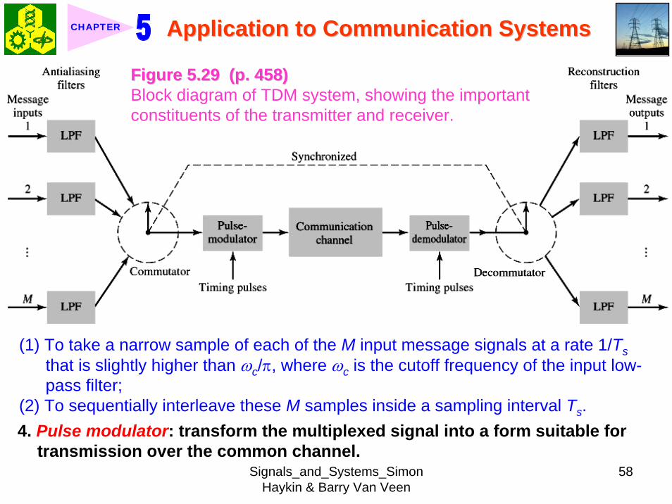
Signals_and_Systems_Simon Haykin amp Barry Van Veen
59
Application to Communication SystemsApplication to Communication SystemsCHAPTER
clubs The use of time-division multiplexing introduces a bandwidth expansion factor M because the scheme must squeeze M samples derived from M independent message sources into a time slot equal to one sampling interval
5 Pulse demodulator performs the inverse operation of the pulse modulator6 Decommutator distributes the narrow samples produced by pulse demodulator to the appropriate low-pass reconstruction filter7 Synchronization between the timing operations of the transmitter and
receiver in a TDM system is essential for satisfactory performance of the system
Inserting an extra pulse into each sampling interval on a regular basisBandwidth expansion factor is increased to M + 1
clubs The TDM system is hghly sensitive to the dispersion in the common transmission channel
Example 57 Comparison of TDM with FDMATDM system is used to multiplex four independent voice signals using PAM Each voice signal is sampled at the rate of 8 kHz The system incorporates a synchronizing pulse train for its proper operation
Signals_and_Systems_Simon Haykin amp Barry Van Veen
60
Application to Communication SystemsApplication to Communication SystemsCHAPTER
(a) Determine the timing relationships between the synchronizing pulse train and the impulse trains used to sample the four voice signals
(b) Calculate the transmission bandwidth of the channel for the TDM system and compare the result with a corresponding FDM system using SSBmodulation
ltltSolgtSolgt(a) The sampling period is
31 125 s
8 10sT s μ= =times
In this example the number of voice signals is M = 4 Hence dividing the sampling period of 125 μs among these voice signals and the synchronizing pulse train we obtain the time slot allocated to each one of them
0 1125 25 s
5
sTTM
μ
=+
= =
Signals_and_Systems_Simon Haykin amp Barry Van Veen
61
Application to Communication SystemsApplication to Communication SystemsCHAPTER
Figure 530Figure 530 shows the timing relationships between the synchronizing pulse train and the four impulse trains used to sample the different voice signals in a single frame Each frame includes time slots of common duration T0 = 25 μs which are allocated to the pulse-modulated signals and synchronizing pulse
Figure 530 (p 459)Figure 530 (p 459)Composition of one frame of a multiplexed PAM signal incorporating four voice-signals and a synchronizing pulse
Signals_and_Systems_Simon Haykin amp Barry Van Veen
62
Application to Communication SystemsApplication to Communication SystemsCHAPTER
(b) As a consequence of the time-bandwidth product (see Section 317) there is an inverse relationship between the duration of a pulse and the bandwidth (ie cutoff frequency) of the channel needed for itstransmission Accordingly the overall transmission bandwidth of the channel is
0
21 1 MHz 40 kHz
25
TTf
T
ωπ
=
= = =
In contrast the use of an FDM system based on SSB modulation requires a channel bandwidth equal to M times that of a single voice signal-that is 4 X 4 = 16 kHz Thus the use of PAM-TDM requires a channel bandwidth that is 40 16 = 25 times that of SSB-FDMIn practice pulse-code modulation is commonly used as the method of modulation for TDM this results in a further increase in channel bandwidth depending on the length of the code word used in the digital representation of each pulse in the PAM signal
Signals_and_Systems_Simon Haykin amp Barry Van Veen
63
Application to Communication SystemsApplication to Communication SystemsCHAPTER
510 510 Pulse and Group Delays Pulse and Group Delays 1 Whenever a signal is transmitted through a dispersive (ie frequency
selective) system some delay is introduced into the output signal in relation to the input signal
2 The delay is determined by the phase response of the system3 Phase response of a dispersive communication channel
( ) arg ( )H jφ ω ω= (532)
A signal is transmitted through the channel at a frequency ωc The signal received at the channel lags the transmitted signal by φ(ωc) The time delay is called phase delay formally defined as
( )cp
c
φ ωτω
= minus (533)
The phase delay is not necessarily the true signal delayclubs Case study for DSB-SC1 Transmitted signal
0( ) cos( ) cos( )cs t A t tω ω= (534)
ωc equiv carrier frequency ω0 equiv sinusoidal modulation frequency
A = AcA0
Signals_and_Systems_Simon Haykin amp Barry Van Veen
64
Application to Communication SystemsApplication to Communication SystemsCHAPTER
1 21 1( ) cos( ) cos( )2 2
s t A t A tω ω= +
1 0cω ω ω= + (535) where
2 0cω ω ω= minus (536)
Upper frequency
Lower frequency
2 Let the s(t) be transmitted through the channel with phase response φ (ω) Accordingly the signal received at the channel output is
1 1 2 21 1( ) cos( ( )) cos( ( ))2 2
y t A t A tω φ ω ω φ ω= + + +
1 2 1 20
( ) ( ) ( )1 ( )( ) cos cos2 2cy t A t tφ ω φ ω φ ω φ ωω ω+⎛ ⎞ ⎛ ⎞= + +⎜ ⎟ ⎜ ⎟
⎝ ⎠ ⎝ ⎠(537)
3 Two observations from Eq (537)1) The carrier component at frequency ωc in y(t) lags its counterpart in s(t) by
frac12 (φ (ω1) + φ (ω2)) which represents a time delay equal to
1 2 1 2
c 1 2
( )+ ( ) ( )+ ( )2 +
φ ω φ ω φ ω φ ωω ω ω
minus = minus (538)
Signals_and_Systems_Simon Haykin amp Barry Van Veen
65
Application to Communication SystemsApplication to Communication SystemsCHAPTER
2) The message component at frequency ω0 in y(t) lags its counterpart in s(t) by frac12 (φ (ω1) minus φ (ω2)) which represents a time delay equal to
1 2 1 2
0 1 2
( ) ( ) ( ) ( )2
φ ω φ ω φ ω φ ωω ω ωminus minus
minus = minusminus
(539)
4 Suppose that ω0 lt ωc rArr the side frequencies are close together with ω c between them Such a modulated signal is said to be a narrowband signal The phase response φ (ω) in the vicinity of ω = ωc is approximated by two-term Taylor series expansion
( )( ) ( ) ( )c
c cd
d ω ω
φ ωφ ω φ ω ω ωω =
= + times minus (540)
Phase delay = ( ) c cφ ω ωminus
5 The time delay introduced by the message signal (ie he ldquoenveloperdquo of the modulated signal) is given by
( )
c
gd
d ω ω
φ ωτω =
= minus (541) The time delay τg is called the
envelope delay or group delay
Signals_and_Systems_Simon Haykin amp Barry Van Veen
66
Application to Communication SystemsApplication to Communication SystemsCHAPTER
6 When a modulated signal is transmitted through a communication channel there are two different delays to be considered1) The carrier or phase delay τp defined by Eq (533)2) The envelope or group delay τg defined by Eq (541)
clubs The group delay is the true signal delay
Example 58 Phase and Group Delays for Ban-pass Channel
ltltSolgtSolgt
The phase response of a band-pass communication channel is defined by 2 2
1( ) tan c
c
ω ωφ ωωω
minus ⎛ ⎞minus= minus ⎜ ⎟
⎝ ⎠The signal s(t) defined in Eq (534) is transmitted through this channel with
475 radscω = 0 025 radsω =andCalculate (a) the phase delay and (b) the group delay
(a) At ω = ωc φ (ωc) = 0 According to Eq (533) the phase delay τ p is zero (b) Differentiating φ (ω) with respect to ω we get
Signals_and_Systems_Simon Haykin amp Barry Van Veen
67
Application to Communication SystemsApplication to Communication SystemsCHAPTER
2 2
2 2 2 2 2
( )( )( )
c c
c c
dd
ω ω ωφ ωω ω ω ω ω
+= minus
+ minus
Using thing result in Eq (541) we find that the group delay is 2 2 04211
475gc
sτω
= = =
1 One waveform shown as a solid curve was obtained by multiplying the transmitted signal s(t) by the carrier wave cos(ωct)
2 The second waveform shown as a dotted curve was obtained by multiplying the received signal y(t) by the carrier wave cos(ωct)
To display the results obtained in parts (a) and (b) in graphical form Fig 531Fig 531shows a superposition of two waveforms obtained as follows
The figure clearly shows that the carrier (phase) delay τ p is zero and the envelope of the received signal y(t) is lagging behind that of the transmitted signal by τs seconds For the presentation of waveforms in this figure we purposely did not use a filter to suppress the high frequency components resulting from the multiplications described under points 1 and 2 because of the desire to retain a contribution due to the carrier for display
Signals_and_Systems_Simon Haykin amp Barry Van Veen
68
Application to Communication SystemsApplication to Communication SystemsCHAPTER
Figure 531 Figure 531 (p 463)(p 463)Highlighting the zero carrier delay (solid curve) and group delay τg (dotted curve) which are determined in accordance with Example 58
Signals_and_Systems_Simon Haykin amp Barry Van Veen
69
Application to Communication SystemsApplication to Communication SystemsCHAPTER
clubs Not also that the separation between the upper side frequency ω1 = ωc + ω0 = 500 rads and the lower side frequency ω2 = ωc minus ω0 = 450 rads is about 10 of the carrier frequency ωc = 475 rads which justifies referring to the modulated signal in this example as a narrowband signal
5101 5101 Some Practical ConsiderationsSome Practical Considerationsclubs What is the practical importance of group delay 1 Eq (541) for determining group delay applies strictly to narrowband
modulated signal2 The message bandwidth may be comparable to the carrier frequency In
this situation the group delay is formulated as a frequency-dependent parameter ie ( )d( )g d
φ ωτ ωω
= minus (542)
3 When a wideband modulated signals transmitted through a dispersive channel the frequency components of the message signal are delayed by different amounts at the channel output
Delay distortionFig 532Fig 532 Group delay response of voice-grade telephone channel
Signals_and_Systems_Simon Haykin amp Barry Van Veen
70
Application to Communication SystemsApplication to Communication SystemsCHAPTER
Figure 532 (p 464)Group delay response of voice-grade telephone channel (Adapted from J C Bellamy Digital Telephony Wiley 1982)
511 511 Exploring Concepts with MATLABExploring Concepts with MATLAB5111 5111 Full AMFull AMclubs Sinusoidal modulation
clubs To reconstruct a faithful version of the original message signal in the receiver we have to use a delay equalizer
0( ) [1 cos( )]cos( )c cs t A t tμ ω ω= +1 AM experiment
1cA =
08 radscω π= 0 01 radsω π=Carrier amplitude
Carrier frequency Modulation amplitude
Signals_and_Systems_Simon Haykin amp Barry Van Veen
71
Application to Communication SystemsApplication to Communication SystemsCHAPTER
2 We wish to display and analyze 10 full cycles of the AM wave corresponding to a total duration of 200 s Choosing a sampling rate 1Ts = 10 Hz we have a total of N = 2000 time samples The frequency band of interest is minus 10 π ≦ ω ≦ 10 π Since the separation between the carrier and either side frequency is equal to the modulation frequency ω0 = 01 π rads we would like to have a frequency resolution ωr = 001π rads To achieve this resolution we require the following number of frequency samples (see Eq (442))
20 2000001
s
r
M ω πω π
ge = =
3 We therefore choose M = 2000 To approximate the Fourier transform of the AM wave s(t) we may use a 2000-point DTFS The only variable in the AM experiment is the modulation factor μ with respect to which we wish to investigate three different situationsμ = 05 corresponding to under-modulationμ = 10 for which the AM system is on the verge of over-modulationμ = 20 corresponding to over-modulation
Signals_and_Systems_Simon Haykin amp Barry Van Veen
72
Application to Communication SystemsApplication to Communication SystemsCHAPTER
4 MATLAB commandsAc = 1 carrier amplitudewc = 08pi carrier frequencyw0 = 01pi modulation frequencymu = 05 modulation factort = 0011999s = Ac(1 + mucos(w0t))cos(wct)plot(ts)Smag = abs(fftshift(fft(s2000)))2000 Smag denotes the magnitude specturm of the AM wavew = 10[-1000999]2pi2000plot(wSmag)axis ([-30 30 0 08])
5 5 μμ = 05 = 05 case case Fig 533Fig 533μμ = 10 case = 10 case Fig 534Fig 534μμ = 20 case = 20 case Fig 535Fig 535
Discussion see pp 466-469 textbook
Signals_and_Systems_Simon Haykin amp Barry Van Veen
73
Application to Communication SystemsApplication to Communication SystemsCHAPTER
-30 -20 -10 0 10 20 300
02
04
06
0 50 100 150 200-2
-1
0
1
2
2 22 24 26 28 3
02
04
06
(a) Time (s)
Time domain
Frequency domain
(b) Frequency (rads)
Frequency domain
Frequency (rads)
Figure 533 (p 466)Amplitude modulation with 50 modulation (a) AM wave (b) magnitude spectrum of the AM wave and (c) expanded spectrum around the carrier frequency
μμ = 05 = 05 casecase
Signals_and_Systems_Simon Haykin amp Barry Van Veen
74
Application to Communication SystemsApplication to Communication SystemsCHAPTER
Figure 534 (p 467)Figure 534 (p 467)Amplitude modulation with 100 modulation (a) AM wave (b) magnitude spectrum of the AM wave and (c) expanded spectrum around the carrier frequency
Signals_and_Systems_Simon Haykin amp Barry Van Veen
75
Application to Communication SystemsApplication to Communication SystemsCHAPTER
Figure 535 (p 468)Amplitude modulation with 200 modulation (a) AM wave (b) magnitude spectrum of the AM wave and (c) expanded spectrum around the carrier frequency
Signals_and_Systems_Simon Haykin amp Barry Van Veen
76
Application to Communication SystemsApplication to Communication SystemsCHAPTER
5112 5112 DSBDSB--SC ModulationSC Modulation1 Sinusoidal modulation
0 0( ) cos( ) cos( )c cs t A A t tω ω=
2 MATLAB commands
Ac = 1 carrier amplitudewc = 08pi carrier frequency in radsA0 = 1 amplitude of modulating signalw0 = 01pi frequency of modulating signalt = 011999s = AcA0cos(wct)cos(w0t)plot(ts)Smag = abs(fftshift(fft(s2000)))2000w = 10[-1000999]2pi2000plot(wSmag)
3 3 DSBDSB--SC modulated waveSC modulated wave Fig 536Fig 536 Discussion see pp 466-469 textbook
4 Output of the product modulator in Fig 512 (b) with φ = 0
Signals_and_Systems_Simon Haykin amp Barry Van Veen
77
Application to Communication SystemsApplication to Communication SystemsCHAPTER
Figure 536 (p 469)DSB-SC modulation (a) DSB-SC modulated wave (b) magnitude spectrum of the modulated wave and (c) expanded spectrum around the carrier frequency
Signals_and_Systems_Simon Haykin amp Barry Van Veen
78
Application to Communication SystemsApplication to Communication SystemsCHAPTER
( ) ( ) cos( )cv t s t tω=
5 MATLAB commandsgtgt v = scos(wct)
6 Fig 537 (a) waveforms of v(t) Fig 537 (b) magnitude spectrum which readily shows that v(t) consists of the following components1) A sinusoidal component with frequency 01π rads representing the
modulating wave2) A new DSB-SC modulated wave with double carrier frequency of 16π rads
in actuality the side frequencies of this modulated wave are located at 15πand 17π rads
1) The frequency of the modulating wave lies inside the passband of the filter2) The upper and lower side frequencies of the new DSB-SC modulated wave
lie inside the stopband of the filter
Accordingly we may recover the sinusoidal modulating signal by passing v(t) through low-pass filter with the following requirements
Signals_and_Systems_Simon Haykin amp Barry Van Veen
79
Application to Communication SystemsApplication to Communication SystemsCHAPTER
Figure 537 (p 470)Coherent detection of DSB-SC modulated wave (a) and (b) Waveform and magnitude spectrum of signal produced at the output of produce modulator (c) and (d) waveform and magnitude spectrum of low-pass filter output
Signals_and_Systems_Simon Haykin amp Barry Van Veen
80
Application to Communication SystemsApplication to Communication SystemsCHAPTER
The issue of how to design a filter with these requirements will be considered in detail in Chapter 8 For the present it suffices to say that the preceding requirements can be met by using the following MATLAB commands
gtgt [ba] = butter(30025)gtgt output = filter(bav)
The first command produces s special type of filter called a Butterworth filter For the experiment considered here the filter order is 3 and its normalized cutoff frequency of 0025 is calculated as follows
Actual cutoff frequency of filter 025 radsHalf the sampling rate 10 rads
0025
ππ
=
=
The second command computes the filterrsquos output in response to the product modulator output v(t) (We will revisit the design of this filter in Chapter 8) Figure 537(c) displays the waveform of the low-pass filter output this waveform represents a sinusoidal signal of frequency 005 Hz an observation that is confirmed by using the ffr command to approximate the spectrum of the filter output The result of the computation is shown in Fig 537(d)Fig 537(d)
Signals_and_Systems_Simon Haykin amp Barry Van Veen
81
Application to Communication SystemsApplication to Communication SystemsCHAPTER
7 In Fig 538 we explore another aspect of DSB-SC modulation namely the effect of varying the modulation frequency Figure 538(a) shows five cycles of a DSB-SC modulated wave that has the same carrier frequency as that in Fig 536(a) but the modulation frequency has been reduced to 0025 Hz( ie a radian frequency of 005π) Figure 538(b) shows the magnitude spectrum of this second DSB-SC modulated wave and its zoomed-in version is shown in Fig 538(c) Comparing this latter figure with Fig 536(c) we see clearly that decreasing the modulation frequency has the effect of moving the upper and lower side frequencies closer together which is consistent with modulation theory
5113 5113 Phase and Group DelayPhase and Group Delay1 In Example 58 we studied the phase and group delays for a band-pass
channel with phase response 2 2
1( ) tan c
c
ω ωφ ωωω
minus ⎛ ⎞minus= minus ⎜ ⎟
⎝ ⎠2 At ω = ωc the phase delay is τ p = 0 and the group delay is τ s = 04211s One
of the wave forms displayed in Fig 531Fig 531 is
1( ) ( ) cos( )cx t s t tω=
Signals_and_Systems_Simon Haykin amp Barry Van Veen
82
Application to Communication SystemsApplication to Communication SystemsCHAPTER
Figure 538 (p 472)Effect of varying the modulation frequency compared with that in Fig 537 (a) and (b) Waveform and magnitude spectrum of DSB-SC modulated wave with a modulation frequency one-half that used in Fig 536 (c) expanded spectrum around the carrier frequency
Signals_and_Systems_Simon Haykin amp Barry Van Veen
83
Application to Communication SystemsApplication to Communication SystemsCHAPTER
where (see page 461)
1 2( ) [cos( ) cos( )]2As t t tω ω= +
and ω1 = ωc + ω0 and ω2 = ωc - ω0 The waveform shown in the figure as a solid curve is a plot of x1(t) The other waveform also displayed in Fig 531Fig 531 is
2
1 1 2 2
( ) ( ) cos( )
[cos( ( )) cos( ( ))]cos( )2
c
c
x t y t tA t t t
ω
ω φ ω ω φ ω ω
=
= + + +
where the angle φ (ω1) and φ (ω2) are the values of the phase response φ (ω) at ω = ω1 and ω = ω2 respectively The waveform shown as a dotted curve in the figure is a plot of x2(t)
3 The generation of x1(t) and x2(t) in MATLAB is achieved with the following commands with A2 set equal to unity
Signals_and_Systems_Simon Haykin amp Barry Van Veen
84
Application to Communication SystemsApplication to Communication SystemsCHAPTER
wc = 475w0 = 025w1 = wc + w0w2 = wc - w0t = -10 0001 10o1 = -atan((w1^2 - wc^2)(w1wc))o2 = -atan((w2^2 - wc^2)(w2wc))s = cos(w1t) + cos(w2t)y = cos(w1t + o1) + cos(w2t + o2)x1 = scos(478t)x2 = ycos(475t)plot(tx1b)hold on plot(tx2k)hold offxlabel(Time)ylabel(Amplitude)
Note that we have set (A2) = 1 for convenience of presentation The function atan in the first two commands returns the arctangent Note also that the computation of both x1 and x2 involve element-by-element multiplications ndash hence the use of period followed by an asterisk
Signals_and_Systems_Simon Haykin amp Barry Van Veen
85
Application to Communication SystemsApplication to Communication SystemsCHAPTER
Signals_and_Systems_Simon Haykin amp Barry Van Veen
86
Application to Communication SystemsApplication to Communication SystemsCHAPTER
Signals_and_Systems_Simon Haykin amp Barry Van Veen
87
Application to Communication SystemsApplication to Communication SystemsCHAPTER
Signals_and_Systems_Simon Haykin amp Barry Van Veen
60
Application to Communication SystemsApplication to Communication SystemsCHAPTER
(a) Determine the timing relationships between the synchronizing pulse train and the impulse trains used to sample the four voice signals
(b) Calculate the transmission bandwidth of the channel for the TDM system and compare the result with a corresponding FDM system using SSBmodulation
ltltSolgtSolgt(a) The sampling period is
31 125 s
8 10sT s μ= =times
In this example the number of voice signals is M = 4 Hence dividing the sampling period of 125 μs among these voice signals and the synchronizing pulse train we obtain the time slot allocated to each one of them
0 1125 25 s
5
sTTM
μ
=+
= =
Signals_and_Systems_Simon Haykin amp Barry Van Veen
61
Application to Communication SystemsApplication to Communication SystemsCHAPTER
Figure 530Figure 530 shows the timing relationships between the synchronizing pulse train and the four impulse trains used to sample the different voice signals in a single frame Each frame includes time slots of common duration T0 = 25 μs which are allocated to the pulse-modulated signals and synchronizing pulse
Figure 530 (p 459)Figure 530 (p 459)Composition of one frame of a multiplexed PAM signal incorporating four voice-signals and a synchronizing pulse
Signals_and_Systems_Simon Haykin amp Barry Van Veen
62
Application to Communication SystemsApplication to Communication SystemsCHAPTER
(b) As a consequence of the time-bandwidth product (see Section 317) there is an inverse relationship between the duration of a pulse and the bandwidth (ie cutoff frequency) of the channel needed for itstransmission Accordingly the overall transmission bandwidth of the channel is
0
21 1 MHz 40 kHz
25
TTf
T
ωπ
=
= = =
In contrast the use of an FDM system based on SSB modulation requires a channel bandwidth equal to M times that of a single voice signal-that is 4 X 4 = 16 kHz Thus the use of PAM-TDM requires a channel bandwidth that is 40 16 = 25 times that of SSB-FDMIn practice pulse-code modulation is commonly used as the method of modulation for TDM this results in a further increase in channel bandwidth depending on the length of the code word used in the digital representation of each pulse in the PAM signal
Signals_and_Systems_Simon Haykin amp Barry Van Veen
63
Application to Communication SystemsApplication to Communication SystemsCHAPTER
510 510 Pulse and Group Delays Pulse and Group Delays 1 Whenever a signal is transmitted through a dispersive (ie frequency
selective) system some delay is introduced into the output signal in relation to the input signal
2 The delay is determined by the phase response of the system3 Phase response of a dispersive communication channel
( ) arg ( )H jφ ω ω= (532)
A signal is transmitted through the channel at a frequency ωc The signal received at the channel lags the transmitted signal by φ(ωc) The time delay is called phase delay formally defined as
( )cp
c
φ ωτω
= minus (533)
The phase delay is not necessarily the true signal delayclubs Case study for DSB-SC1 Transmitted signal
0( ) cos( ) cos( )cs t A t tω ω= (534)
ωc equiv carrier frequency ω0 equiv sinusoidal modulation frequency
A = AcA0
Signals_and_Systems_Simon Haykin amp Barry Van Veen
64
Application to Communication SystemsApplication to Communication SystemsCHAPTER
1 21 1( ) cos( ) cos( )2 2
s t A t A tω ω= +
1 0cω ω ω= + (535) where
2 0cω ω ω= minus (536)
Upper frequency
Lower frequency
2 Let the s(t) be transmitted through the channel with phase response φ (ω) Accordingly the signal received at the channel output is
1 1 2 21 1( ) cos( ( )) cos( ( ))2 2
y t A t A tω φ ω ω φ ω= + + +
1 2 1 20
( ) ( ) ( )1 ( )( ) cos cos2 2cy t A t tφ ω φ ω φ ω φ ωω ω+⎛ ⎞ ⎛ ⎞= + +⎜ ⎟ ⎜ ⎟
⎝ ⎠ ⎝ ⎠(537)
3 Two observations from Eq (537)1) The carrier component at frequency ωc in y(t) lags its counterpart in s(t) by
frac12 (φ (ω1) + φ (ω2)) which represents a time delay equal to
1 2 1 2
c 1 2
( )+ ( ) ( )+ ( )2 +
φ ω φ ω φ ω φ ωω ω ω
minus = minus (538)
Signals_and_Systems_Simon Haykin amp Barry Van Veen
65
Application to Communication SystemsApplication to Communication SystemsCHAPTER
2) The message component at frequency ω0 in y(t) lags its counterpart in s(t) by frac12 (φ (ω1) minus φ (ω2)) which represents a time delay equal to
1 2 1 2
0 1 2
( ) ( ) ( ) ( )2
φ ω φ ω φ ω φ ωω ω ωminus minus
minus = minusminus
(539)
4 Suppose that ω0 lt ωc rArr the side frequencies are close together with ω c between them Such a modulated signal is said to be a narrowband signal The phase response φ (ω) in the vicinity of ω = ωc is approximated by two-term Taylor series expansion
( )( ) ( ) ( )c
c cd
d ω ω
φ ωφ ω φ ω ω ωω =
= + times minus (540)
Phase delay = ( ) c cφ ω ωminus
5 The time delay introduced by the message signal (ie he ldquoenveloperdquo of the modulated signal) is given by
( )
c
gd
d ω ω
φ ωτω =
= minus (541) The time delay τg is called the
envelope delay or group delay
Signals_and_Systems_Simon Haykin amp Barry Van Veen
66
Application to Communication SystemsApplication to Communication SystemsCHAPTER
6 When a modulated signal is transmitted through a communication channel there are two different delays to be considered1) The carrier or phase delay τp defined by Eq (533)2) The envelope or group delay τg defined by Eq (541)
clubs The group delay is the true signal delay
Example 58 Phase and Group Delays for Ban-pass Channel
ltltSolgtSolgt
The phase response of a band-pass communication channel is defined by 2 2
1( ) tan c
c
ω ωφ ωωω
minus ⎛ ⎞minus= minus ⎜ ⎟
⎝ ⎠The signal s(t) defined in Eq (534) is transmitted through this channel with
475 radscω = 0 025 radsω =andCalculate (a) the phase delay and (b) the group delay
(a) At ω = ωc φ (ωc) = 0 According to Eq (533) the phase delay τ p is zero (b) Differentiating φ (ω) with respect to ω we get
Signals_and_Systems_Simon Haykin amp Barry Van Veen
67
Application to Communication SystemsApplication to Communication SystemsCHAPTER
2 2
2 2 2 2 2
( )( )( )
c c
c c
dd
ω ω ωφ ωω ω ω ω ω
+= minus
+ minus
Using thing result in Eq (541) we find that the group delay is 2 2 04211
475gc
sτω
= = =
1 One waveform shown as a solid curve was obtained by multiplying the transmitted signal s(t) by the carrier wave cos(ωct)
2 The second waveform shown as a dotted curve was obtained by multiplying the received signal y(t) by the carrier wave cos(ωct)
To display the results obtained in parts (a) and (b) in graphical form Fig 531Fig 531shows a superposition of two waveforms obtained as follows
The figure clearly shows that the carrier (phase) delay τ p is zero and the envelope of the received signal y(t) is lagging behind that of the transmitted signal by τs seconds For the presentation of waveforms in this figure we purposely did not use a filter to suppress the high frequency components resulting from the multiplications described under points 1 and 2 because of the desire to retain a contribution due to the carrier for display
Signals_and_Systems_Simon Haykin amp Barry Van Veen
68
Application to Communication SystemsApplication to Communication SystemsCHAPTER
Figure 531 Figure 531 (p 463)(p 463)Highlighting the zero carrier delay (solid curve) and group delay τg (dotted curve) which are determined in accordance with Example 58
Signals_and_Systems_Simon Haykin amp Barry Van Veen
69
Application to Communication SystemsApplication to Communication SystemsCHAPTER
clubs Not also that the separation between the upper side frequency ω1 = ωc + ω0 = 500 rads and the lower side frequency ω2 = ωc minus ω0 = 450 rads is about 10 of the carrier frequency ωc = 475 rads which justifies referring to the modulated signal in this example as a narrowband signal
5101 5101 Some Practical ConsiderationsSome Practical Considerationsclubs What is the practical importance of group delay 1 Eq (541) for determining group delay applies strictly to narrowband
modulated signal2 The message bandwidth may be comparable to the carrier frequency In
this situation the group delay is formulated as a frequency-dependent parameter ie ( )d( )g d
φ ωτ ωω
= minus (542)
3 When a wideband modulated signals transmitted through a dispersive channel the frequency components of the message signal are delayed by different amounts at the channel output
Delay distortionFig 532Fig 532 Group delay response of voice-grade telephone channel
Signals_and_Systems_Simon Haykin amp Barry Van Veen
70
Application to Communication SystemsApplication to Communication SystemsCHAPTER
Figure 532 (p 464)Group delay response of voice-grade telephone channel (Adapted from J C Bellamy Digital Telephony Wiley 1982)
511 511 Exploring Concepts with MATLABExploring Concepts with MATLAB5111 5111 Full AMFull AMclubs Sinusoidal modulation
clubs To reconstruct a faithful version of the original message signal in the receiver we have to use a delay equalizer
0( ) [1 cos( )]cos( )c cs t A t tμ ω ω= +1 AM experiment
1cA =
08 radscω π= 0 01 radsω π=Carrier amplitude
Carrier frequency Modulation amplitude
Signals_and_Systems_Simon Haykin amp Barry Van Veen
71
Application to Communication SystemsApplication to Communication SystemsCHAPTER
2 We wish to display and analyze 10 full cycles of the AM wave corresponding to a total duration of 200 s Choosing a sampling rate 1Ts = 10 Hz we have a total of N = 2000 time samples The frequency band of interest is minus 10 π ≦ ω ≦ 10 π Since the separation between the carrier and either side frequency is equal to the modulation frequency ω0 = 01 π rads we would like to have a frequency resolution ωr = 001π rads To achieve this resolution we require the following number of frequency samples (see Eq (442))
20 2000001
s
r
M ω πω π
ge = =
3 We therefore choose M = 2000 To approximate the Fourier transform of the AM wave s(t) we may use a 2000-point DTFS The only variable in the AM experiment is the modulation factor μ with respect to which we wish to investigate three different situationsμ = 05 corresponding to under-modulationμ = 10 for which the AM system is on the verge of over-modulationμ = 20 corresponding to over-modulation
Signals_and_Systems_Simon Haykin amp Barry Van Veen
72
Application to Communication SystemsApplication to Communication SystemsCHAPTER
4 MATLAB commandsAc = 1 carrier amplitudewc = 08pi carrier frequencyw0 = 01pi modulation frequencymu = 05 modulation factort = 0011999s = Ac(1 + mucos(w0t))cos(wct)plot(ts)Smag = abs(fftshift(fft(s2000)))2000 Smag denotes the magnitude specturm of the AM wavew = 10[-1000999]2pi2000plot(wSmag)axis ([-30 30 0 08])
5 5 μμ = 05 = 05 case case Fig 533Fig 533μμ = 10 case = 10 case Fig 534Fig 534μμ = 20 case = 20 case Fig 535Fig 535
Discussion see pp 466-469 textbook
Signals_and_Systems_Simon Haykin amp Barry Van Veen
73
Application to Communication SystemsApplication to Communication SystemsCHAPTER
-30 -20 -10 0 10 20 300
02
04
06
0 50 100 150 200-2
-1
0
1
2
2 22 24 26 28 3
02
04
06
(a) Time (s)
Time domain
Frequency domain
(b) Frequency (rads)
Frequency domain
Frequency (rads)
Figure 533 (p 466)Amplitude modulation with 50 modulation (a) AM wave (b) magnitude spectrum of the AM wave and (c) expanded spectrum around the carrier frequency
μμ = 05 = 05 casecase
Signals_and_Systems_Simon Haykin amp Barry Van Veen
74
Application to Communication SystemsApplication to Communication SystemsCHAPTER
Figure 534 (p 467)Figure 534 (p 467)Amplitude modulation with 100 modulation (a) AM wave (b) magnitude spectrum of the AM wave and (c) expanded spectrum around the carrier frequency
Signals_and_Systems_Simon Haykin amp Barry Van Veen
75
Application to Communication SystemsApplication to Communication SystemsCHAPTER
Figure 535 (p 468)Amplitude modulation with 200 modulation (a) AM wave (b) magnitude spectrum of the AM wave and (c) expanded spectrum around the carrier frequency
Signals_and_Systems_Simon Haykin amp Barry Van Veen
76
Application to Communication SystemsApplication to Communication SystemsCHAPTER
5112 5112 DSBDSB--SC ModulationSC Modulation1 Sinusoidal modulation
0 0( ) cos( ) cos( )c cs t A A t tω ω=
2 MATLAB commands
Ac = 1 carrier amplitudewc = 08pi carrier frequency in radsA0 = 1 amplitude of modulating signalw0 = 01pi frequency of modulating signalt = 011999s = AcA0cos(wct)cos(w0t)plot(ts)Smag = abs(fftshift(fft(s2000)))2000w = 10[-1000999]2pi2000plot(wSmag)
3 3 DSBDSB--SC modulated waveSC modulated wave Fig 536Fig 536 Discussion see pp 466-469 textbook
4 Output of the product modulator in Fig 512 (b) with φ = 0
Signals_and_Systems_Simon Haykin amp Barry Van Veen
77
Application to Communication SystemsApplication to Communication SystemsCHAPTER
Figure 536 (p 469)DSB-SC modulation (a) DSB-SC modulated wave (b) magnitude spectrum of the modulated wave and (c) expanded spectrum around the carrier frequency
Signals_and_Systems_Simon Haykin amp Barry Van Veen
78
Application to Communication SystemsApplication to Communication SystemsCHAPTER
( ) ( ) cos( )cv t s t tω=
5 MATLAB commandsgtgt v = scos(wct)
6 Fig 537 (a) waveforms of v(t) Fig 537 (b) magnitude spectrum which readily shows that v(t) consists of the following components1) A sinusoidal component with frequency 01π rads representing the
modulating wave2) A new DSB-SC modulated wave with double carrier frequency of 16π rads
in actuality the side frequencies of this modulated wave are located at 15πand 17π rads
1) The frequency of the modulating wave lies inside the passband of the filter2) The upper and lower side frequencies of the new DSB-SC modulated wave
lie inside the stopband of the filter
Accordingly we may recover the sinusoidal modulating signal by passing v(t) through low-pass filter with the following requirements
Signals_and_Systems_Simon Haykin amp Barry Van Veen
79
Application to Communication SystemsApplication to Communication SystemsCHAPTER
Figure 537 (p 470)Coherent detection of DSB-SC modulated wave (a) and (b) Waveform and magnitude spectrum of signal produced at the output of produce modulator (c) and (d) waveform and magnitude spectrum of low-pass filter output
Signals_and_Systems_Simon Haykin amp Barry Van Veen
80
Application to Communication SystemsApplication to Communication SystemsCHAPTER
The issue of how to design a filter with these requirements will be considered in detail in Chapter 8 For the present it suffices to say that the preceding requirements can be met by using the following MATLAB commands
gtgt [ba] = butter(30025)gtgt output = filter(bav)
The first command produces s special type of filter called a Butterworth filter For the experiment considered here the filter order is 3 and its normalized cutoff frequency of 0025 is calculated as follows
Actual cutoff frequency of filter 025 radsHalf the sampling rate 10 rads
0025
ππ
=
=
The second command computes the filterrsquos output in response to the product modulator output v(t) (We will revisit the design of this filter in Chapter 8) Figure 537(c) displays the waveform of the low-pass filter output this waveform represents a sinusoidal signal of frequency 005 Hz an observation that is confirmed by using the ffr command to approximate the spectrum of the filter output The result of the computation is shown in Fig 537(d)Fig 537(d)
Signals_and_Systems_Simon Haykin amp Barry Van Veen
81
Application to Communication SystemsApplication to Communication SystemsCHAPTER
7 In Fig 538 we explore another aspect of DSB-SC modulation namely the effect of varying the modulation frequency Figure 538(a) shows five cycles of a DSB-SC modulated wave that has the same carrier frequency as that in Fig 536(a) but the modulation frequency has been reduced to 0025 Hz( ie a radian frequency of 005π) Figure 538(b) shows the magnitude spectrum of this second DSB-SC modulated wave and its zoomed-in version is shown in Fig 538(c) Comparing this latter figure with Fig 536(c) we see clearly that decreasing the modulation frequency has the effect of moving the upper and lower side frequencies closer together which is consistent with modulation theory
5113 5113 Phase and Group DelayPhase and Group Delay1 In Example 58 we studied the phase and group delays for a band-pass
channel with phase response 2 2
1( ) tan c
c
ω ωφ ωωω
minus ⎛ ⎞minus= minus ⎜ ⎟
⎝ ⎠2 At ω = ωc the phase delay is τ p = 0 and the group delay is τ s = 04211s One
of the wave forms displayed in Fig 531Fig 531 is
1( ) ( ) cos( )cx t s t tω=
Signals_and_Systems_Simon Haykin amp Barry Van Veen
82
Application to Communication SystemsApplication to Communication SystemsCHAPTER
Figure 538 (p 472)Effect of varying the modulation frequency compared with that in Fig 537 (a) and (b) Waveform and magnitude spectrum of DSB-SC modulated wave with a modulation frequency one-half that used in Fig 536 (c) expanded spectrum around the carrier frequency
Signals_and_Systems_Simon Haykin amp Barry Van Veen
83
Application to Communication SystemsApplication to Communication SystemsCHAPTER
where (see page 461)
1 2( ) [cos( ) cos( )]2As t t tω ω= +
and ω1 = ωc + ω0 and ω2 = ωc - ω0 The waveform shown in the figure as a solid curve is a plot of x1(t) The other waveform also displayed in Fig 531Fig 531 is
2
1 1 2 2
( ) ( ) cos( )
[cos( ( )) cos( ( ))]cos( )2
c
c
x t y t tA t t t
ω
ω φ ω ω φ ω ω
=
= + + +
where the angle φ (ω1) and φ (ω2) are the values of the phase response φ (ω) at ω = ω1 and ω = ω2 respectively The waveform shown as a dotted curve in the figure is a plot of x2(t)
3 The generation of x1(t) and x2(t) in MATLAB is achieved with the following commands with A2 set equal to unity
Signals_and_Systems_Simon Haykin amp Barry Van Veen
84
Application to Communication SystemsApplication to Communication SystemsCHAPTER
wc = 475w0 = 025w1 = wc + w0w2 = wc - w0t = -10 0001 10o1 = -atan((w1^2 - wc^2)(w1wc))o2 = -atan((w2^2 - wc^2)(w2wc))s = cos(w1t) + cos(w2t)y = cos(w1t + o1) + cos(w2t + o2)x1 = scos(478t)x2 = ycos(475t)plot(tx1b)hold on plot(tx2k)hold offxlabel(Time)ylabel(Amplitude)
Note that we have set (A2) = 1 for convenience of presentation The function atan in the first two commands returns the arctangent Note also that the computation of both x1 and x2 involve element-by-element multiplications ndash hence the use of period followed by an asterisk
Signals_and_Systems_Simon Haykin amp Barry Van Veen
85
Application to Communication SystemsApplication to Communication SystemsCHAPTER
Signals_and_Systems_Simon Haykin amp Barry Van Veen
86
Application to Communication SystemsApplication to Communication SystemsCHAPTER
Signals_and_Systems_Simon Haykin amp Barry Van Veen
87
Application to Communication SystemsApplication to Communication SystemsCHAPTER
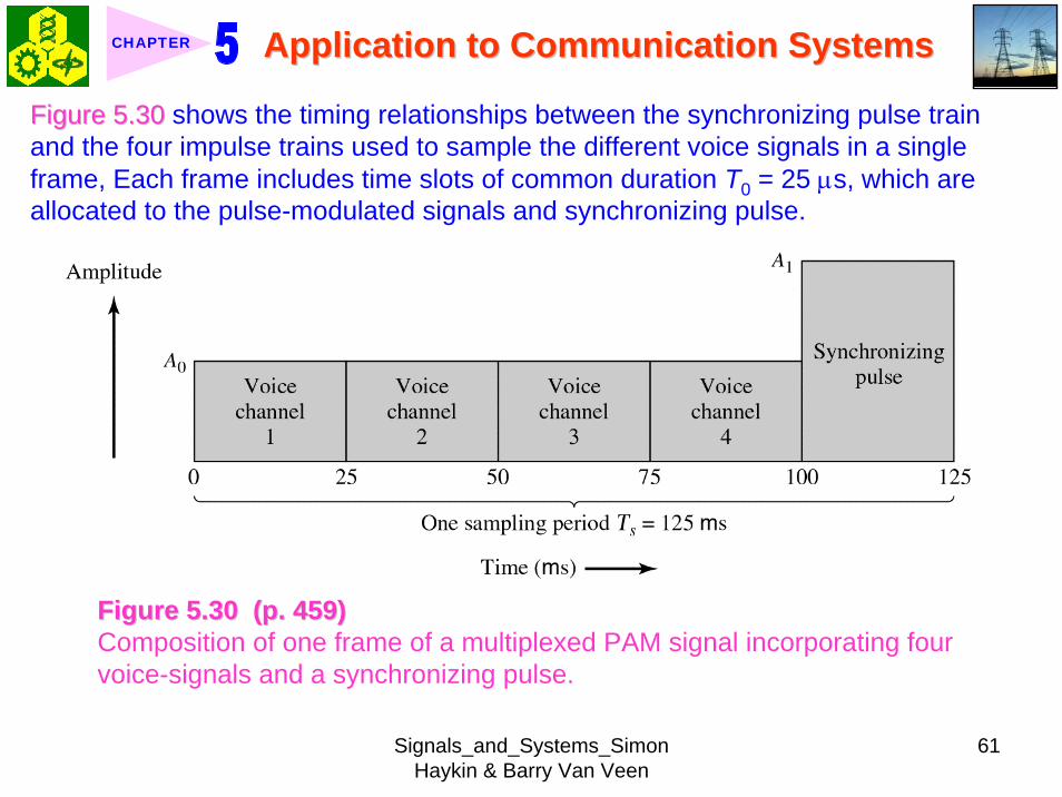
Signals_and_Systems_Simon Haykin amp Barry Van Veen
61
Application to Communication SystemsApplication to Communication SystemsCHAPTER
Figure 530Figure 530 shows the timing relationships between the synchronizing pulse train and the four impulse trains used to sample the different voice signals in a single frame Each frame includes time slots of common duration T0 = 25 μs which are allocated to the pulse-modulated signals and synchronizing pulse
Figure 530 (p 459)Figure 530 (p 459)Composition of one frame of a multiplexed PAM signal incorporating four voice-signals and a synchronizing pulse
Signals_and_Systems_Simon Haykin amp Barry Van Veen
62
Application to Communication SystemsApplication to Communication SystemsCHAPTER
(b) As a consequence of the time-bandwidth product (see Section 317) there is an inverse relationship between the duration of a pulse and the bandwidth (ie cutoff frequency) of the channel needed for itstransmission Accordingly the overall transmission bandwidth of the channel is
0
21 1 MHz 40 kHz
25
TTf
T
ωπ
=
= = =
In contrast the use of an FDM system based on SSB modulation requires a channel bandwidth equal to M times that of a single voice signal-that is 4 X 4 = 16 kHz Thus the use of PAM-TDM requires a channel bandwidth that is 40 16 = 25 times that of SSB-FDMIn practice pulse-code modulation is commonly used as the method of modulation for TDM this results in a further increase in channel bandwidth depending on the length of the code word used in the digital representation of each pulse in the PAM signal
Signals_and_Systems_Simon Haykin amp Barry Van Veen
63
Application to Communication SystemsApplication to Communication SystemsCHAPTER
510 510 Pulse and Group Delays Pulse and Group Delays 1 Whenever a signal is transmitted through a dispersive (ie frequency
selective) system some delay is introduced into the output signal in relation to the input signal
2 The delay is determined by the phase response of the system3 Phase response of a dispersive communication channel
( ) arg ( )H jφ ω ω= (532)
A signal is transmitted through the channel at a frequency ωc The signal received at the channel lags the transmitted signal by φ(ωc) The time delay is called phase delay formally defined as
( )cp
c
φ ωτω
= minus (533)
The phase delay is not necessarily the true signal delayclubs Case study for DSB-SC1 Transmitted signal
0( ) cos( ) cos( )cs t A t tω ω= (534)
ωc equiv carrier frequency ω0 equiv sinusoidal modulation frequency
A = AcA0
Signals_and_Systems_Simon Haykin amp Barry Van Veen
64
Application to Communication SystemsApplication to Communication SystemsCHAPTER
1 21 1( ) cos( ) cos( )2 2
s t A t A tω ω= +
1 0cω ω ω= + (535) where
2 0cω ω ω= minus (536)
Upper frequency
Lower frequency
2 Let the s(t) be transmitted through the channel with phase response φ (ω) Accordingly the signal received at the channel output is
1 1 2 21 1( ) cos( ( )) cos( ( ))2 2
y t A t A tω φ ω ω φ ω= + + +
1 2 1 20
( ) ( ) ( )1 ( )( ) cos cos2 2cy t A t tφ ω φ ω φ ω φ ωω ω+⎛ ⎞ ⎛ ⎞= + +⎜ ⎟ ⎜ ⎟
⎝ ⎠ ⎝ ⎠(537)
3 Two observations from Eq (537)1) The carrier component at frequency ωc in y(t) lags its counterpart in s(t) by
frac12 (φ (ω1) + φ (ω2)) which represents a time delay equal to
1 2 1 2
c 1 2
( )+ ( ) ( )+ ( )2 +
φ ω φ ω φ ω φ ωω ω ω
minus = minus (538)
Signals_and_Systems_Simon Haykin amp Barry Van Veen
65
Application to Communication SystemsApplication to Communication SystemsCHAPTER
2) The message component at frequency ω0 in y(t) lags its counterpart in s(t) by frac12 (φ (ω1) minus φ (ω2)) which represents a time delay equal to
1 2 1 2
0 1 2
( ) ( ) ( ) ( )2
φ ω φ ω φ ω φ ωω ω ωminus minus
minus = minusminus
(539)
4 Suppose that ω0 lt ωc rArr the side frequencies are close together with ω c between them Such a modulated signal is said to be a narrowband signal The phase response φ (ω) in the vicinity of ω = ωc is approximated by two-term Taylor series expansion
( )( ) ( ) ( )c
c cd
d ω ω
φ ωφ ω φ ω ω ωω =
= + times minus (540)
Phase delay = ( ) c cφ ω ωminus
5 The time delay introduced by the message signal (ie he ldquoenveloperdquo of the modulated signal) is given by
( )
c
gd
d ω ω
φ ωτω =
= minus (541) The time delay τg is called the
envelope delay or group delay
Signals_and_Systems_Simon Haykin amp Barry Van Veen
66
Application to Communication SystemsApplication to Communication SystemsCHAPTER
6 When a modulated signal is transmitted through a communication channel there are two different delays to be considered1) The carrier or phase delay τp defined by Eq (533)2) The envelope or group delay τg defined by Eq (541)
clubs The group delay is the true signal delay
Example 58 Phase and Group Delays for Ban-pass Channel
ltltSolgtSolgt
The phase response of a band-pass communication channel is defined by 2 2
1( ) tan c
c
ω ωφ ωωω
minus ⎛ ⎞minus= minus ⎜ ⎟
⎝ ⎠The signal s(t) defined in Eq (534) is transmitted through this channel with
475 radscω = 0 025 radsω =andCalculate (a) the phase delay and (b) the group delay
(a) At ω = ωc φ (ωc) = 0 According to Eq (533) the phase delay τ p is zero (b) Differentiating φ (ω) with respect to ω we get
Signals_and_Systems_Simon Haykin amp Barry Van Veen
67
Application to Communication SystemsApplication to Communication SystemsCHAPTER
2 2
2 2 2 2 2
( )( )( )
c c
c c
dd
ω ω ωφ ωω ω ω ω ω
+= minus
+ minus
Using thing result in Eq (541) we find that the group delay is 2 2 04211
475gc
sτω
= = =
1 One waveform shown as a solid curve was obtained by multiplying the transmitted signal s(t) by the carrier wave cos(ωct)
2 The second waveform shown as a dotted curve was obtained by multiplying the received signal y(t) by the carrier wave cos(ωct)
To display the results obtained in parts (a) and (b) in graphical form Fig 531Fig 531shows a superposition of two waveforms obtained as follows
The figure clearly shows that the carrier (phase) delay τ p is zero and the envelope of the received signal y(t) is lagging behind that of the transmitted signal by τs seconds For the presentation of waveforms in this figure we purposely did not use a filter to suppress the high frequency components resulting from the multiplications described under points 1 and 2 because of the desire to retain a contribution due to the carrier for display
Signals_and_Systems_Simon Haykin amp Barry Van Veen
68
Application to Communication SystemsApplication to Communication SystemsCHAPTER
Figure 531 Figure 531 (p 463)(p 463)Highlighting the zero carrier delay (solid curve) and group delay τg (dotted curve) which are determined in accordance with Example 58
Signals_and_Systems_Simon Haykin amp Barry Van Veen
69
Application to Communication SystemsApplication to Communication SystemsCHAPTER
clubs Not also that the separation between the upper side frequency ω1 = ωc + ω0 = 500 rads and the lower side frequency ω2 = ωc minus ω0 = 450 rads is about 10 of the carrier frequency ωc = 475 rads which justifies referring to the modulated signal in this example as a narrowband signal
5101 5101 Some Practical ConsiderationsSome Practical Considerationsclubs What is the practical importance of group delay 1 Eq (541) for determining group delay applies strictly to narrowband
modulated signal2 The message bandwidth may be comparable to the carrier frequency In
this situation the group delay is formulated as a frequency-dependent parameter ie ( )d( )g d
φ ωτ ωω
= minus (542)
3 When a wideband modulated signals transmitted through a dispersive channel the frequency components of the message signal are delayed by different amounts at the channel output
Delay distortionFig 532Fig 532 Group delay response of voice-grade telephone channel
Signals_and_Systems_Simon Haykin amp Barry Van Veen
70
Application to Communication SystemsApplication to Communication SystemsCHAPTER
Figure 532 (p 464)Group delay response of voice-grade telephone channel (Adapted from J C Bellamy Digital Telephony Wiley 1982)
511 511 Exploring Concepts with MATLABExploring Concepts with MATLAB5111 5111 Full AMFull AMclubs Sinusoidal modulation
clubs To reconstruct a faithful version of the original message signal in the receiver we have to use a delay equalizer
0( ) [1 cos( )]cos( )c cs t A t tμ ω ω= +1 AM experiment
1cA =
08 radscω π= 0 01 radsω π=Carrier amplitude
Carrier frequency Modulation amplitude
Signals_and_Systems_Simon Haykin amp Barry Van Veen
71
Application to Communication SystemsApplication to Communication SystemsCHAPTER
2 We wish to display and analyze 10 full cycles of the AM wave corresponding to a total duration of 200 s Choosing a sampling rate 1Ts = 10 Hz we have a total of N = 2000 time samples The frequency band of interest is minus 10 π ≦ ω ≦ 10 π Since the separation between the carrier and either side frequency is equal to the modulation frequency ω0 = 01 π rads we would like to have a frequency resolution ωr = 001π rads To achieve this resolution we require the following number of frequency samples (see Eq (442))
20 2000001
s
r
M ω πω π
ge = =
3 We therefore choose M = 2000 To approximate the Fourier transform of the AM wave s(t) we may use a 2000-point DTFS The only variable in the AM experiment is the modulation factor μ with respect to which we wish to investigate three different situationsμ = 05 corresponding to under-modulationμ = 10 for which the AM system is on the verge of over-modulationμ = 20 corresponding to over-modulation
Signals_and_Systems_Simon Haykin amp Barry Van Veen
72
Application to Communication SystemsApplication to Communication SystemsCHAPTER
4 MATLAB commandsAc = 1 carrier amplitudewc = 08pi carrier frequencyw0 = 01pi modulation frequencymu = 05 modulation factort = 0011999s = Ac(1 + mucos(w0t))cos(wct)plot(ts)Smag = abs(fftshift(fft(s2000)))2000 Smag denotes the magnitude specturm of the AM wavew = 10[-1000999]2pi2000plot(wSmag)axis ([-30 30 0 08])
5 5 μμ = 05 = 05 case case Fig 533Fig 533μμ = 10 case = 10 case Fig 534Fig 534μμ = 20 case = 20 case Fig 535Fig 535
Discussion see pp 466-469 textbook
Signals_and_Systems_Simon Haykin amp Barry Van Veen
73
Application to Communication SystemsApplication to Communication SystemsCHAPTER
-30 -20 -10 0 10 20 300
02
04
06
0 50 100 150 200-2
-1
0
1
2
2 22 24 26 28 3
02
04
06
(a) Time (s)
Time domain
Frequency domain
(b) Frequency (rads)
Frequency domain
Frequency (rads)
Figure 533 (p 466)Amplitude modulation with 50 modulation (a) AM wave (b) magnitude spectrum of the AM wave and (c) expanded spectrum around the carrier frequency
μμ = 05 = 05 casecase
Signals_and_Systems_Simon Haykin amp Barry Van Veen
74
Application to Communication SystemsApplication to Communication SystemsCHAPTER
Figure 534 (p 467)Figure 534 (p 467)Amplitude modulation with 100 modulation (a) AM wave (b) magnitude spectrum of the AM wave and (c) expanded spectrum around the carrier frequency
Signals_and_Systems_Simon Haykin amp Barry Van Veen
75
Application to Communication SystemsApplication to Communication SystemsCHAPTER
Figure 535 (p 468)Amplitude modulation with 200 modulation (a) AM wave (b) magnitude spectrum of the AM wave and (c) expanded spectrum around the carrier frequency
Signals_and_Systems_Simon Haykin amp Barry Van Veen
76
Application to Communication SystemsApplication to Communication SystemsCHAPTER
5112 5112 DSBDSB--SC ModulationSC Modulation1 Sinusoidal modulation
0 0( ) cos( ) cos( )c cs t A A t tω ω=
2 MATLAB commands
Ac = 1 carrier amplitudewc = 08pi carrier frequency in radsA0 = 1 amplitude of modulating signalw0 = 01pi frequency of modulating signalt = 011999s = AcA0cos(wct)cos(w0t)plot(ts)Smag = abs(fftshift(fft(s2000)))2000w = 10[-1000999]2pi2000plot(wSmag)
3 3 DSBDSB--SC modulated waveSC modulated wave Fig 536Fig 536 Discussion see pp 466-469 textbook
4 Output of the product modulator in Fig 512 (b) with φ = 0
Signals_and_Systems_Simon Haykin amp Barry Van Veen
77
Application to Communication SystemsApplication to Communication SystemsCHAPTER
Figure 536 (p 469)DSB-SC modulation (a) DSB-SC modulated wave (b) magnitude spectrum of the modulated wave and (c) expanded spectrum around the carrier frequency
Signals_and_Systems_Simon Haykin amp Barry Van Veen
78
Application to Communication SystemsApplication to Communication SystemsCHAPTER
( ) ( ) cos( )cv t s t tω=
5 MATLAB commandsgtgt v = scos(wct)
6 Fig 537 (a) waveforms of v(t) Fig 537 (b) magnitude spectrum which readily shows that v(t) consists of the following components1) A sinusoidal component with frequency 01π rads representing the
modulating wave2) A new DSB-SC modulated wave with double carrier frequency of 16π rads
in actuality the side frequencies of this modulated wave are located at 15πand 17π rads
1) The frequency of the modulating wave lies inside the passband of the filter2) The upper and lower side frequencies of the new DSB-SC modulated wave
lie inside the stopband of the filter
Accordingly we may recover the sinusoidal modulating signal by passing v(t) through low-pass filter with the following requirements
Signals_and_Systems_Simon Haykin amp Barry Van Veen
79
Application to Communication SystemsApplication to Communication SystemsCHAPTER
Figure 537 (p 470)Coherent detection of DSB-SC modulated wave (a) and (b) Waveform and magnitude spectrum of signal produced at the output of produce modulator (c) and (d) waveform and magnitude spectrum of low-pass filter output
Signals_and_Systems_Simon Haykin amp Barry Van Veen
80
Application to Communication SystemsApplication to Communication SystemsCHAPTER
The issue of how to design a filter with these requirements will be considered in detail in Chapter 8 For the present it suffices to say that the preceding requirements can be met by using the following MATLAB commands
gtgt [ba] = butter(30025)gtgt output = filter(bav)
The first command produces s special type of filter called a Butterworth filter For the experiment considered here the filter order is 3 and its normalized cutoff frequency of 0025 is calculated as follows
Actual cutoff frequency of filter 025 radsHalf the sampling rate 10 rads
0025
ππ
=
=
The second command computes the filterrsquos output in response to the product modulator output v(t) (We will revisit the design of this filter in Chapter 8) Figure 537(c) displays the waveform of the low-pass filter output this waveform represents a sinusoidal signal of frequency 005 Hz an observation that is confirmed by using the ffr command to approximate the spectrum of the filter output The result of the computation is shown in Fig 537(d)Fig 537(d)
Signals_and_Systems_Simon Haykin amp Barry Van Veen
81
Application to Communication SystemsApplication to Communication SystemsCHAPTER
7 In Fig 538 we explore another aspect of DSB-SC modulation namely the effect of varying the modulation frequency Figure 538(a) shows five cycles of a DSB-SC modulated wave that has the same carrier frequency as that in Fig 536(a) but the modulation frequency has been reduced to 0025 Hz( ie a radian frequency of 005π) Figure 538(b) shows the magnitude spectrum of this second DSB-SC modulated wave and its zoomed-in version is shown in Fig 538(c) Comparing this latter figure with Fig 536(c) we see clearly that decreasing the modulation frequency has the effect of moving the upper and lower side frequencies closer together which is consistent with modulation theory
5113 5113 Phase and Group DelayPhase and Group Delay1 In Example 58 we studied the phase and group delays for a band-pass
channel with phase response 2 2
1( ) tan c
c
ω ωφ ωωω
minus ⎛ ⎞minus= minus ⎜ ⎟
⎝ ⎠2 At ω = ωc the phase delay is τ p = 0 and the group delay is τ s = 04211s One
of the wave forms displayed in Fig 531Fig 531 is
1( ) ( ) cos( )cx t s t tω=
Signals_and_Systems_Simon Haykin amp Barry Van Veen
82
Application to Communication SystemsApplication to Communication SystemsCHAPTER
Figure 538 (p 472)Effect of varying the modulation frequency compared with that in Fig 537 (a) and (b) Waveform and magnitude spectrum of DSB-SC modulated wave with a modulation frequency one-half that used in Fig 536 (c) expanded spectrum around the carrier frequency
Signals_and_Systems_Simon Haykin amp Barry Van Veen
83
Application to Communication SystemsApplication to Communication SystemsCHAPTER
where (see page 461)
1 2( ) [cos( ) cos( )]2As t t tω ω= +
and ω1 = ωc + ω0 and ω2 = ωc - ω0 The waveform shown in the figure as a solid curve is a plot of x1(t) The other waveform also displayed in Fig 531Fig 531 is
2
1 1 2 2
( ) ( ) cos( )
[cos( ( )) cos( ( ))]cos( )2
c
c
x t y t tA t t t
ω
ω φ ω ω φ ω ω
=
= + + +
where the angle φ (ω1) and φ (ω2) are the values of the phase response φ (ω) at ω = ω1 and ω = ω2 respectively The waveform shown as a dotted curve in the figure is a plot of x2(t)
3 The generation of x1(t) and x2(t) in MATLAB is achieved with the following commands with A2 set equal to unity
Signals_and_Systems_Simon Haykin amp Barry Van Veen
84
Application to Communication SystemsApplication to Communication SystemsCHAPTER
wc = 475w0 = 025w1 = wc + w0w2 = wc - w0t = -10 0001 10o1 = -atan((w1^2 - wc^2)(w1wc))o2 = -atan((w2^2 - wc^2)(w2wc))s = cos(w1t) + cos(w2t)y = cos(w1t + o1) + cos(w2t + o2)x1 = scos(478t)x2 = ycos(475t)plot(tx1b)hold on plot(tx2k)hold offxlabel(Time)ylabel(Amplitude)
Note that we have set (A2) = 1 for convenience of presentation The function atan in the first two commands returns the arctangent Note also that the computation of both x1 and x2 involve element-by-element multiplications ndash hence the use of period followed by an asterisk
Signals_and_Systems_Simon Haykin amp Barry Van Veen
85
Application to Communication SystemsApplication to Communication SystemsCHAPTER
Signals_and_Systems_Simon Haykin amp Barry Van Veen
86
Application to Communication SystemsApplication to Communication SystemsCHAPTER
Signals_and_Systems_Simon Haykin amp Barry Van Veen
87
Application to Communication SystemsApplication to Communication SystemsCHAPTER
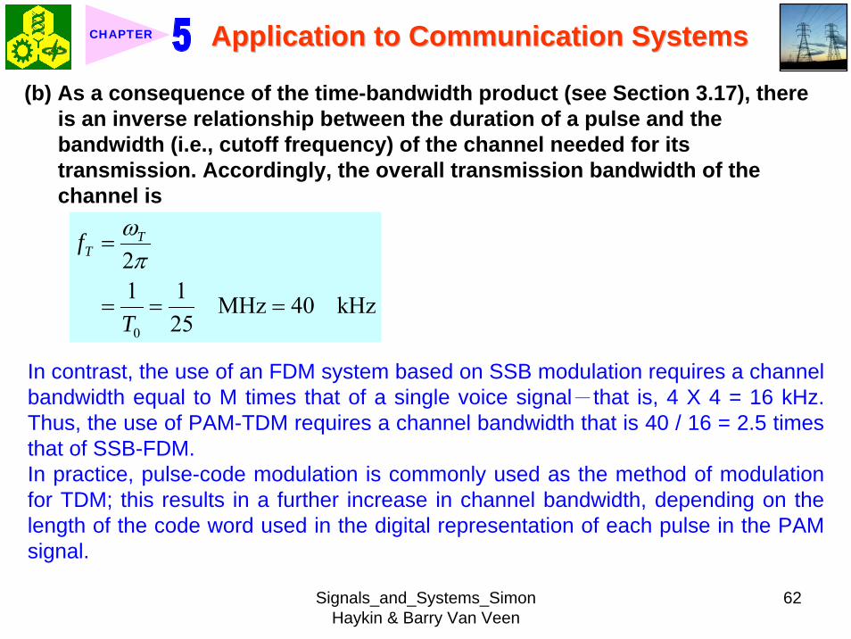
Signals_and_Systems_Simon Haykin amp Barry Van Veen
66
Application to Communication SystemsApplication to Communication SystemsCHAPTER
6 When a modulated signal is transmitted through a communication channel there are two different delays to be considered1) The carrier or phase delay τp defined by Eq (533)2) The envelope or group delay τg defined by Eq (541)
clubs The group delay is the true signal delay
Example 58 Phase and Group Delays for Ban-pass Channel
ltltSolgtSolgt
The phase response of a band-pass communication channel is defined by 2 2
1( ) tan c
c
ω ωφ ωωω
minus ⎛ ⎞minus= minus ⎜ ⎟
⎝ ⎠The signal s(t) defined in Eq (534) is transmitted through this channel with
475 radscω = 0 025 radsω =andCalculate (a) the phase delay and (b) the group delay
(a) At ω = ωc φ (ωc) = 0 According to Eq (533) the phase delay τ p is zero (b) Differentiating φ (ω) with respect to ω we get
Signals_and_Systems_Simon Haykin amp Barry Van Veen
67
Application to Communication SystemsApplication to Communication SystemsCHAPTER
2 2
2 2 2 2 2
( )( )( )
c c
c c
dd
ω ω ωφ ωω ω ω ω ω
+= minus
+ minus
Using thing result in Eq (541) we find that the group delay is 2 2 04211
475gc
sτω
= = =
1 One waveform shown as a solid curve was obtained by multiplying the transmitted signal s(t) by the carrier wave cos(ωct)
2 The second waveform shown as a dotted curve was obtained by multiplying the received signal y(t) by the carrier wave cos(ωct)
To display the results obtained in parts (a) and (b) in graphical form Fig 531Fig 531shows a superposition of two waveforms obtained as follows
The figure clearly shows that the carrier (phase) delay τ p is zero and the envelope of the received signal y(t) is lagging behind that of the transmitted signal by τs seconds For the presentation of waveforms in this figure we purposely did not use a filter to suppress the high frequency components resulting from the multiplications described under points 1 and 2 because of the desire to retain a contribution due to the carrier for display
Signals_and_Systems_Simon Haykin amp Barry Van Veen
68
Application to Communication SystemsApplication to Communication SystemsCHAPTER
Figure 531 Figure 531 (p 463)(p 463)Highlighting the zero carrier delay (solid curve) and group delay τg (dotted curve) which are determined in accordance with Example 58
Signals_and_Systems_Simon Haykin amp Barry Van Veen
69
Application to Communication SystemsApplication to Communication SystemsCHAPTER
clubs Not also that the separation between the upper side frequency ω1 = ωc + ω0 = 500 rads and the lower side frequency ω2 = ωc minus ω0 = 450 rads is about 10 of the carrier frequency ωc = 475 rads which justifies referring to the modulated signal in this example as a narrowband signal
5101 5101 Some Practical ConsiderationsSome Practical Considerationsclubs What is the practical importance of group delay 1 Eq (541) for determining group delay applies strictly to narrowband
modulated signal2 The message bandwidth may be comparable to the carrier frequency In
this situation the group delay is formulated as a frequency-dependent parameter ie ( )d( )g d
φ ωτ ωω
= minus (542)
3 When a wideband modulated signals transmitted through a dispersive channel the frequency components of the message signal are delayed by different amounts at the channel output
Delay distortionFig 532Fig 532 Group delay response of voice-grade telephone channel
Signals_and_Systems_Simon Haykin amp Barry Van Veen
70
Application to Communication SystemsApplication to Communication SystemsCHAPTER
Figure 532 (p 464)Group delay response of voice-grade telephone channel (Adapted from J C Bellamy Digital Telephony Wiley 1982)
511 511 Exploring Concepts with MATLABExploring Concepts with MATLAB5111 5111 Full AMFull AMclubs Sinusoidal modulation
clubs To reconstruct a faithful version of the original message signal in the receiver we have to use a delay equalizer
0( ) [1 cos( )]cos( )c cs t A t tμ ω ω= +1 AM experiment
1cA =
08 radscω π= 0 01 radsω π=Carrier amplitude
Carrier frequency Modulation amplitude
Signals_and_Systems_Simon Haykin amp Barry Van Veen
71
Application to Communication SystemsApplication to Communication SystemsCHAPTER
2 We wish to display and analyze 10 full cycles of the AM wave corresponding to a total duration of 200 s Choosing a sampling rate 1Ts = 10 Hz we have a total of N = 2000 time samples The frequency band of interest is minus 10 π ≦ ω ≦ 10 π Since the separation between the carrier and either side frequency is equal to the modulation frequency ω0 = 01 π rads we would like to have a frequency resolution ωr = 001π rads To achieve this resolution we require the following number of frequency samples (see Eq (442))
20 2000001
s
r
M ω πω π
ge = =
3 We therefore choose M = 2000 To approximate the Fourier transform of the AM wave s(t) we may use a 2000-point DTFS The only variable in the AM experiment is the modulation factor μ with respect to which we wish to investigate three different situationsμ = 05 corresponding to under-modulationμ = 10 for which the AM system is on the verge of over-modulationμ = 20 corresponding to over-modulation
Signals_and_Systems_Simon Haykin amp Barry Van Veen
72
Application to Communication SystemsApplication to Communication SystemsCHAPTER
4 MATLAB commandsAc = 1 carrier amplitudewc = 08pi carrier frequencyw0 = 01pi modulation frequencymu = 05 modulation factort = 0011999s = Ac(1 + mucos(w0t))cos(wct)plot(ts)Smag = abs(fftshift(fft(s2000)))2000 Smag denotes the magnitude specturm of the AM wavew = 10[-1000999]2pi2000plot(wSmag)axis ([-30 30 0 08])
5 5 μμ = 05 = 05 case case Fig 533Fig 533μμ = 10 case = 10 case Fig 534Fig 534μμ = 20 case = 20 case Fig 535Fig 535
Discussion see pp 466-469 textbook
Signals_and_Systems_Simon Haykin amp Barry Van Veen
73
Application to Communication SystemsApplication to Communication SystemsCHAPTER
-30 -20 -10 0 10 20 300
02
04
06
0 50 100 150 200-2
-1
0
1
2
2 22 24 26 28 3
02
04
06
(a) Time (s)
Time domain
Frequency domain
(b) Frequency (rads)
Frequency domain
Frequency (rads)
Figure 533 (p 466)Amplitude modulation with 50 modulation (a) AM wave (b) magnitude spectrum of the AM wave and (c) expanded spectrum around the carrier frequency
μμ = 05 = 05 casecase
Signals_and_Systems_Simon Haykin amp Barry Van Veen
74
Application to Communication SystemsApplication to Communication SystemsCHAPTER
Figure 534 (p 467)Figure 534 (p 467)Amplitude modulation with 100 modulation (a) AM wave (b) magnitude spectrum of the AM wave and (c) expanded spectrum around the carrier frequency
Signals_and_Systems_Simon Haykin amp Barry Van Veen
75
Application to Communication SystemsApplication to Communication SystemsCHAPTER
Figure 535 (p 468)Amplitude modulation with 200 modulation (a) AM wave (b) magnitude spectrum of the AM wave and (c) expanded spectrum around the carrier frequency
Signals_and_Systems_Simon Haykin amp Barry Van Veen
76
Application to Communication SystemsApplication to Communication SystemsCHAPTER
5112 5112 DSBDSB--SC ModulationSC Modulation1 Sinusoidal modulation
0 0( ) cos( ) cos( )c cs t A A t tω ω=
2 MATLAB commands
Ac = 1 carrier amplitudewc = 08pi carrier frequency in radsA0 = 1 amplitude of modulating signalw0 = 01pi frequency of modulating signalt = 011999s = AcA0cos(wct)cos(w0t)plot(ts)Smag = abs(fftshift(fft(s2000)))2000w = 10[-1000999]2pi2000plot(wSmag)
3 3 DSBDSB--SC modulated waveSC modulated wave Fig 536Fig 536 Discussion see pp 466-469 textbook
4 Output of the product modulator in Fig 512 (b) with φ = 0
Signals_and_Systems_Simon Haykin amp Barry Van Veen
77
Application to Communication SystemsApplication to Communication SystemsCHAPTER
Figure 536 (p 469)DSB-SC modulation (a) DSB-SC modulated wave (b) magnitude spectrum of the modulated wave and (c) expanded spectrum around the carrier frequency
Signals_and_Systems_Simon Haykin amp Barry Van Veen
78
Application to Communication SystemsApplication to Communication SystemsCHAPTER
( ) ( ) cos( )cv t s t tω=
5 MATLAB commandsgtgt v = scos(wct)
6 Fig 537 (a) waveforms of v(t) Fig 537 (b) magnitude spectrum which readily shows that v(t) consists of the following components1) A sinusoidal component with frequency 01π rads representing the
modulating wave2) A new DSB-SC modulated wave with double carrier frequency of 16π rads
in actuality the side frequencies of this modulated wave are located at 15πand 17π rads
1) The frequency of the modulating wave lies inside the passband of the filter2) The upper and lower side frequencies of the new DSB-SC modulated wave
lie inside the stopband of the filter
Accordingly we may recover the sinusoidal modulating signal by passing v(t) through low-pass filter with the following requirements
Signals_and_Systems_Simon Haykin amp Barry Van Veen
79
Application to Communication SystemsApplication to Communication SystemsCHAPTER
Figure 537 (p 470)Coherent detection of DSB-SC modulated wave (a) and (b) Waveform and magnitude spectrum of signal produced at the output of produce modulator (c) and (d) waveform and magnitude spectrum of low-pass filter output
Signals_and_Systems_Simon Haykin amp Barry Van Veen
80
Application to Communication SystemsApplication to Communication SystemsCHAPTER
The issue of how to design a filter with these requirements will be considered in detail in Chapter 8 For the present it suffices to say that the preceding requirements can be met by using the following MATLAB commands
gtgt [ba] = butter(30025)gtgt output = filter(bav)
The first command produces s special type of filter called a Butterworth filter For the experiment considered here the filter order is 3 and its normalized cutoff frequency of 0025 is calculated as follows
Actual cutoff frequency of filter 025 radsHalf the sampling rate 10 rads
0025
ππ
=
=
The second command computes the filterrsquos output in response to the product modulator output v(t) (We will revisit the design of this filter in Chapter 8) Figure 537(c) displays the waveform of the low-pass filter output this waveform represents a sinusoidal signal of frequency 005 Hz an observation that is confirmed by using the ffr command to approximate the spectrum of the filter output The result of the computation is shown in Fig 537(d)Fig 537(d)
Signals_and_Systems_Simon Haykin amp Barry Van Veen
81
Application to Communication SystemsApplication to Communication SystemsCHAPTER
7 In Fig 538 we explore another aspect of DSB-SC modulation namely the effect of varying the modulation frequency Figure 538(a) shows five cycles of a DSB-SC modulated wave that has the same carrier frequency as that in Fig 536(a) but the modulation frequency has been reduced to 0025 Hz( ie a radian frequency of 005π) Figure 538(b) shows the magnitude spectrum of this second DSB-SC modulated wave and its zoomed-in version is shown in Fig 538(c) Comparing this latter figure with Fig 536(c) we see clearly that decreasing the modulation frequency has the effect of moving the upper and lower side frequencies closer together which is consistent with modulation theory
5113 5113 Phase and Group DelayPhase and Group Delay1 In Example 58 we studied the phase and group delays for a band-pass
channel with phase response 2 2
1( ) tan c
c
ω ωφ ωωω
minus ⎛ ⎞minus= minus ⎜ ⎟
⎝ ⎠2 At ω = ωc the phase delay is τ p = 0 and the group delay is τ s = 04211s One
of the wave forms displayed in Fig 531Fig 531 is
1( ) ( ) cos( )cx t s t tω=
Signals_and_Systems_Simon Haykin amp Barry Van Veen
82
Application to Communication SystemsApplication to Communication SystemsCHAPTER
Figure 538 (p 472)Effect of varying the modulation frequency compared with that in Fig 537 (a) and (b) Waveform and magnitude spectrum of DSB-SC modulated wave with a modulation frequency one-half that used in Fig 536 (c) expanded spectrum around the carrier frequency
Signals_and_Systems_Simon Haykin amp Barry Van Veen
83
Application to Communication SystemsApplication to Communication SystemsCHAPTER
where (see page 461)
1 2( ) [cos( ) cos( )]2As t t tω ω= +
and ω1 = ωc + ω0 and ω2 = ωc - ω0 The waveform shown in the figure as a solid curve is a plot of x1(t) The other waveform also displayed in Fig 531Fig 531 is
2
1 1 2 2
( ) ( ) cos( )
[cos( ( )) cos( ( ))]cos( )2
c
c
x t y t tA t t t
ω
ω φ ω ω φ ω ω
=
= + + +
where the angle φ (ω1) and φ (ω2) are the values of the phase response φ (ω) at ω = ω1 and ω = ω2 respectively The waveform shown as a dotted curve in the figure is a plot of x2(t)
3 The generation of x1(t) and x2(t) in MATLAB is achieved with the following commands with A2 set equal to unity
Signals_and_Systems_Simon Haykin amp Barry Van Veen
84
Application to Communication SystemsApplication to Communication SystemsCHAPTER
wc = 475w0 = 025w1 = wc + w0w2 = wc - w0t = -10 0001 10o1 = -atan((w1^2 - wc^2)(w1wc))o2 = -atan((w2^2 - wc^2)(w2wc))s = cos(w1t) + cos(w2t)y = cos(w1t + o1) + cos(w2t + o2)x1 = scos(478t)x2 = ycos(475t)plot(tx1b)hold on plot(tx2k)hold offxlabel(Time)ylabel(Amplitude)
Note that we have set (A2) = 1 for convenience of presentation The function atan in the first two commands returns the arctangent Note also that the computation of both x1 and x2 involve element-by-element multiplications ndash hence the use of period followed by an asterisk
Signals_and_Systems_Simon Haykin amp Barry Van Veen
85
Application to Communication SystemsApplication to Communication SystemsCHAPTER
Signals_and_Systems_Simon Haykin amp Barry Van Veen
86
Application to Communication SystemsApplication to Communication SystemsCHAPTER
Signals_and_Systems_Simon Haykin amp Barry Van Veen
87
Application to Communication SystemsApplication to Communication SystemsCHAPTER
Signals_and_Systems_Simon Haykin amp Barry Van Veen
67
Application to Communication SystemsApplication to Communication SystemsCHAPTER
2 2
2 2 2 2 2
( )( )( )
c c
c c
dd
ω ω ωφ ωω ω ω ω ω
+= minus
+ minus
Using thing result in Eq (541) we find that the group delay is 2 2 04211
475gc
sτω
= = =
1 One waveform shown as a solid curve was obtained by multiplying the transmitted signal s(t) by the carrier wave cos(ωct)
2 The second waveform shown as a dotted curve was obtained by multiplying the received signal y(t) by the carrier wave cos(ωct)
To display the results obtained in parts (a) and (b) in graphical form Fig 531Fig 531shows a superposition of two waveforms obtained as follows
The figure clearly shows that the carrier (phase) delay τ p is zero and the envelope of the received signal y(t) is lagging behind that of the transmitted signal by τs seconds For the presentation of waveforms in this figure we purposely did not use a filter to suppress the high frequency components resulting from the multiplications described under points 1 and 2 because of the desire to retain a contribution due to the carrier for display
Signals_and_Systems_Simon Haykin amp Barry Van Veen
68
Application to Communication SystemsApplication to Communication SystemsCHAPTER
Figure 531 Figure 531 (p 463)(p 463)Highlighting the zero carrier delay (solid curve) and group delay τg (dotted curve) which are determined in accordance with Example 58
Signals_and_Systems_Simon Haykin amp Barry Van Veen
69
Application to Communication SystemsApplication to Communication SystemsCHAPTER
clubs Not also that the separation between the upper side frequency ω1 = ωc + ω0 = 500 rads and the lower side frequency ω2 = ωc minus ω0 = 450 rads is about 10 of the carrier frequency ωc = 475 rads which justifies referring to the modulated signal in this example as a narrowband signal
5101 5101 Some Practical ConsiderationsSome Practical Considerationsclubs What is the practical importance of group delay 1 Eq (541) for determining group delay applies strictly to narrowband
modulated signal2 The message bandwidth may be comparable to the carrier frequency In
this situation the group delay is formulated as a frequency-dependent parameter ie ( )d( )g d
φ ωτ ωω
= minus (542)
3 When a wideband modulated signals transmitted through a dispersive channel the frequency components of the message signal are delayed by different amounts at the channel output
Delay distortionFig 532Fig 532 Group delay response of voice-grade telephone channel
Signals_and_Systems_Simon Haykin amp Barry Van Veen
70
Application to Communication SystemsApplication to Communication SystemsCHAPTER
Figure 532 (p 464)Group delay response of voice-grade telephone channel (Adapted from J C Bellamy Digital Telephony Wiley 1982)
511 511 Exploring Concepts with MATLABExploring Concepts with MATLAB5111 5111 Full AMFull AMclubs Sinusoidal modulation
clubs To reconstruct a faithful version of the original message signal in the receiver we have to use a delay equalizer
0( ) [1 cos( )]cos( )c cs t A t tμ ω ω= +1 AM experiment
1cA =
08 radscω π= 0 01 radsω π=Carrier amplitude
Carrier frequency Modulation amplitude
Signals_and_Systems_Simon Haykin amp Barry Van Veen
71
Application to Communication SystemsApplication to Communication SystemsCHAPTER
2 We wish to display and analyze 10 full cycles of the AM wave corresponding to a total duration of 200 s Choosing a sampling rate 1Ts = 10 Hz we have a total of N = 2000 time samples The frequency band of interest is minus 10 π ≦ ω ≦ 10 π Since the separation between the carrier and either side frequency is equal to the modulation frequency ω0 = 01 π rads we would like to have a frequency resolution ωr = 001π rads To achieve this resolution we require the following number of frequency samples (see Eq (442))
20 2000001
s
r
M ω πω π
ge = =
3 We therefore choose M = 2000 To approximate the Fourier transform of the AM wave s(t) we may use a 2000-point DTFS The only variable in the AM experiment is the modulation factor μ with respect to which we wish to investigate three different situationsμ = 05 corresponding to under-modulationμ = 10 for which the AM system is on the verge of over-modulationμ = 20 corresponding to over-modulation
Signals_and_Systems_Simon Haykin amp Barry Van Veen
72
Application to Communication SystemsApplication to Communication SystemsCHAPTER
4 MATLAB commandsAc = 1 carrier amplitudewc = 08pi carrier frequencyw0 = 01pi modulation frequencymu = 05 modulation factort = 0011999s = Ac(1 + mucos(w0t))cos(wct)plot(ts)Smag = abs(fftshift(fft(s2000)))2000 Smag denotes the magnitude specturm of the AM wavew = 10[-1000999]2pi2000plot(wSmag)axis ([-30 30 0 08])
5 5 μμ = 05 = 05 case case Fig 533Fig 533μμ = 10 case = 10 case Fig 534Fig 534μμ = 20 case = 20 case Fig 535Fig 535
Discussion see pp 466-469 textbook
Signals_and_Systems_Simon Haykin amp Barry Van Veen
73
Application to Communication SystemsApplication to Communication SystemsCHAPTER
-30 -20 -10 0 10 20 300
02
04
06
0 50 100 150 200-2
-1
0
1
2
2 22 24 26 28 3
02
04
06
(a) Time (s)
Time domain
Frequency domain
(b) Frequency (rads)
Frequency domain
Frequency (rads)
Figure 533 (p 466)Amplitude modulation with 50 modulation (a) AM wave (b) magnitude spectrum of the AM wave and (c) expanded spectrum around the carrier frequency
μμ = 05 = 05 casecase
Signals_and_Systems_Simon Haykin amp Barry Van Veen
74
Application to Communication SystemsApplication to Communication SystemsCHAPTER
Figure 534 (p 467)Figure 534 (p 467)Amplitude modulation with 100 modulation (a) AM wave (b) magnitude spectrum of the AM wave and (c) expanded spectrum around the carrier frequency
Signals_and_Systems_Simon Haykin amp Barry Van Veen
75
Application to Communication SystemsApplication to Communication SystemsCHAPTER
Figure 535 (p 468)Amplitude modulation with 200 modulation (a) AM wave (b) magnitude spectrum of the AM wave and (c) expanded spectrum around the carrier frequency
Signals_and_Systems_Simon Haykin amp Barry Van Veen
76
Application to Communication SystemsApplication to Communication SystemsCHAPTER
5112 5112 DSBDSB--SC ModulationSC Modulation1 Sinusoidal modulation
0 0( ) cos( ) cos( )c cs t A A t tω ω=
2 MATLAB commands
Ac = 1 carrier amplitudewc = 08pi carrier frequency in radsA0 = 1 amplitude of modulating signalw0 = 01pi frequency of modulating signalt = 011999s = AcA0cos(wct)cos(w0t)plot(ts)Smag = abs(fftshift(fft(s2000)))2000w = 10[-1000999]2pi2000plot(wSmag)
3 3 DSBDSB--SC modulated waveSC modulated wave Fig 536Fig 536 Discussion see pp 466-469 textbook
4 Output of the product modulator in Fig 512 (b) with φ = 0
Signals_and_Systems_Simon Haykin amp Barry Van Veen
77
Application to Communication SystemsApplication to Communication SystemsCHAPTER
Figure 536 (p 469)DSB-SC modulation (a) DSB-SC modulated wave (b) magnitude spectrum of the modulated wave and (c) expanded spectrum around the carrier frequency
Signals_and_Systems_Simon Haykin amp Barry Van Veen
78
Application to Communication SystemsApplication to Communication SystemsCHAPTER
( ) ( ) cos( )cv t s t tω=
5 MATLAB commandsgtgt v = scos(wct)
6 Fig 537 (a) waveforms of v(t) Fig 537 (b) magnitude spectrum which readily shows that v(t) consists of the following components1) A sinusoidal component with frequency 01π rads representing the
modulating wave2) A new DSB-SC modulated wave with double carrier frequency of 16π rads
in actuality the side frequencies of this modulated wave are located at 15πand 17π rads
1) The frequency of the modulating wave lies inside the passband of the filter2) The upper and lower side frequencies of the new DSB-SC modulated wave
lie inside the stopband of the filter
Accordingly we may recover the sinusoidal modulating signal by passing v(t) through low-pass filter with the following requirements
Signals_and_Systems_Simon Haykin amp Barry Van Veen
79
Application to Communication SystemsApplication to Communication SystemsCHAPTER
Figure 537 (p 470)Coherent detection of DSB-SC modulated wave (a) and (b) Waveform and magnitude spectrum of signal produced at the output of produce modulator (c) and (d) waveform and magnitude spectrum of low-pass filter output
Signals_and_Systems_Simon Haykin amp Barry Van Veen
80
Application to Communication SystemsApplication to Communication SystemsCHAPTER
The issue of how to design a filter with these requirements will be considered in detail in Chapter 8 For the present it suffices to say that the preceding requirements can be met by using the following MATLAB commands
gtgt [ba] = butter(30025)gtgt output = filter(bav)
The first command produces s special type of filter called a Butterworth filter For the experiment considered here the filter order is 3 and its normalized cutoff frequency of 0025 is calculated as follows
Actual cutoff frequency of filter 025 radsHalf the sampling rate 10 rads
0025
ππ
=
=
The second command computes the filterrsquos output in response to the product modulator output v(t) (We will revisit the design of this filter in Chapter 8) Figure 537(c) displays the waveform of the low-pass filter output this waveform represents a sinusoidal signal of frequency 005 Hz an observation that is confirmed by using the ffr command to approximate the spectrum of the filter output The result of the computation is shown in Fig 537(d)Fig 537(d)
Signals_and_Systems_Simon Haykin amp Barry Van Veen
81
Application to Communication SystemsApplication to Communication SystemsCHAPTER
7 In Fig 538 we explore another aspect of DSB-SC modulation namely the effect of varying the modulation frequency Figure 538(a) shows five cycles of a DSB-SC modulated wave that has the same carrier frequency as that in Fig 536(a) but the modulation frequency has been reduced to 0025 Hz( ie a radian frequency of 005π) Figure 538(b) shows the magnitude spectrum of this second DSB-SC modulated wave and its zoomed-in version is shown in Fig 538(c) Comparing this latter figure with Fig 536(c) we see clearly that decreasing the modulation frequency has the effect of moving the upper and lower side frequencies closer together which is consistent with modulation theory
5113 5113 Phase and Group DelayPhase and Group Delay1 In Example 58 we studied the phase and group delays for a band-pass
channel with phase response 2 2
1( ) tan c
c
ω ωφ ωωω
minus ⎛ ⎞minus= minus ⎜ ⎟
⎝ ⎠2 At ω = ωc the phase delay is τ p = 0 and the group delay is τ s = 04211s One
of the wave forms displayed in Fig 531Fig 531 is
1( ) ( ) cos( )cx t s t tω=
Signals_and_Systems_Simon Haykin amp Barry Van Veen
82
Application to Communication SystemsApplication to Communication SystemsCHAPTER
Figure 538 (p 472)Effect of varying the modulation frequency compared with that in Fig 537 (a) and (b) Waveform and magnitude spectrum of DSB-SC modulated wave with a modulation frequency one-half that used in Fig 536 (c) expanded spectrum around the carrier frequency
Signals_and_Systems_Simon Haykin amp Barry Van Veen
83
Application to Communication SystemsApplication to Communication SystemsCHAPTER
where (see page 461)
1 2( ) [cos( ) cos( )]2As t t tω ω= +
and ω1 = ωc + ω0 and ω2 = ωc - ω0 The waveform shown in the figure as a solid curve is a plot of x1(t) The other waveform also displayed in Fig 531Fig 531 is
2
1 1 2 2
( ) ( ) cos( )
[cos( ( )) cos( ( ))]cos( )2
c
c
x t y t tA t t t
ω
ω φ ω ω φ ω ω
=
= + + +
where the angle φ (ω1) and φ (ω2) are the values of the phase response φ (ω) at ω = ω1 and ω = ω2 respectively The waveform shown as a dotted curve in the figure is a plot of x2(t)
3 The generation of x1(t) and x2(t) in MATLAB is achieved with the following commands with A2 set equal to unity
Signals_and_Systems_Simon Haykin amp Barry Van Veen
84
Application to Communication SystemsApplication to Communication SystemsCHAPTER
wc = 475w0 = 025w1 = wc + w0w2 = wc - w0t = -10 0001 10o1 = -atan((w1^2 - wc^2)(w1wc))o2 = -atan((w2^2 - wc^2)(w2wc))s = cos(w1t) + cos(w2t)y = cos(w1t + o1) + cos(w2t + o2)x1 = scos(478t)x2 = ycos(475t)plot(tx1b)hold on plot(tx2k)hold offxlabel(Time)ylabel(Amplitude)
Note that we have set (A2) = 1 for convenience of presentation The function atan in the first two commands returns the arctangent Note also that the computation of both x1 and x2 involve element-by-element multiplications ndash hence the use of period followed by an asterisk
Signals_and_Systems_Simon Haykin amp Barry Van Veen
85
Application to Communication SystemsApplication to Communication SystemsCHAPTER
Signals_and_Systems_Simon Haykin amp Barry Van Veen
86
Application to Communication SystemsApplication to Communication SystemsCHAPTER
Signals_and_Systems_Simon Haykin amp Barry Van Veen
87
Application to Communication SystemsApplication to Communication SystemsCHAPTER

Signals_and_Systems_Simon Haykin amp Barry Van Veen
68
Application to Communication SystemsApplication to Communication SystemsCHAPTER
Figure 531 Figure 531 (p 463)(p 463)Highlighting the zero carrier delay (solid curve) and group delay τg (dotted curve) which are determined in accordance with Example 58
Signals_and_Systems_Simon Haykin amp Barry Van Veen
69
Application to Communication SystemsApplication to Communication SystemsCHAPTER
clubs Not also that the separation between the upper side frequency ω1 = ωc + ω0 = 500 rads and the lower side frequency ω2 = ωc minus ω0 = 450 rads is about 10 of the carrier frequency ωc = 475 rads which justifies referring to the modulated signal in this example as a narrowband signal
5101 5101 Some Practical ConsiderationsSome Practical Considerationsclubs What is the practical importance of group delay 1 Eq (541) for determining group delay applies strictly to narrowband
modulated signal2 The message bandwidth may be comparable to the carrier frequency In
this situation the group delay is formulated as a frequency-dependent parameter ie ( )d( )g d
φ ωτ ωω
= minus (542)
3 When a wideband modulated signals transmitted through a dispersive channel the frequency components of the message signal are delayed by different amounts at the channel output
Delay distortionFig 532Fig 532 Group delay response of voice-grade telephone channel
Signals_and_Systems_Simon Haykin amp Barry Van Veen
70
Application to Communication SystemsApplication to Communication SystemsCHAPTER
Figure 532 (p 464)Group delay response of voice-grade telephone channel (Adapted from J C Bellamy Digital Telephony Wiley 1982)
511 511 Exploring Concepts with MATLABExploring Concepts with MATLAB5111 5111 Full AMFull AMclubs Sinusoidal modulation
clubs To reconstruct a faithful version of the original message signal in the receiver we have to use a delay equalizer
0( ) [1 cos( )]cos( )c cs t A t tμ ω ω= +1 AM experiment
1cA =
08 radscω π= 0 01 radsω π=Carrier amplitude
Carrier frequency Modulation amplitude
Signals_and_Systems_Simon Haykin amp Barry Van Veen
71
Application to Communication SystemsApplication to Communication SystemsCHAPTER
2 We wish to display and analyze 10 full cycles of the AM wave corresponding to a total duration of 200 s Choosing a sampling rate 1Ts = 10 Hz we have a total of N = 2000 time samples The frequency band of interest is minus 10 π ≦ ω ≦ 10 π Since the separation between the carrier and either side frequency is equal to the modulation frequency ω0 = 01 π rads we would like to have a frequency resolution ωr = 001π rads To achieve this resolution we require the following number of frequency samples (see Eq (442))
20 2000001
s
r
M ω πω π
ge = =
3 We therefore choose M = 2000 To approximate the Fourier transform of the AM wave s(t) we may use a 2000-point DTFS The only variable in the AM experiment is the modulation factor μ with respect to which we wish to investigate three different situationsμ = 05 corresponding to under-modulationμ = 10 for which the AM system is on the verge of over-modulationμ = 20 corresponding to over-modulation
Signals_and_Systems_Simon Haykin amp Barry Van Veen
72
Application to Communication SystemsApplication to Communication SystemsCHAPTER
4 MATLAB commandsAc = 1 carrier amplitudewc = 08pi carrier frequencyw0 = 01pi modulation frequencymu = 05 modulation factort = 0011999s = Ac(1 + mucos(w0t))cos(wct)plot(ts)Smag = abs(fftshift(fft(s2000)))2000 Smag denotes the magnitude specturm of the AM wavew = 10[-1000999]2pi2000plot(wSmag)axis ([-30 30 0 08])
5 5 μμ = 05 = 05 case case Fig 533Fig 533μμ = 10 case = 10 case Fig 534Fig 534μμ = 20 case = 20 case Fig 535Fig 535
Discussion see pp 466-469 textbook
Signals_and_Systems_Simon Haykin amp Barry Van Veen
73
Application to Communication SystemsApplication to Communication SystemsCHAPTER
-30 -20 -10 0 10 20 300
02
04
06
0 50 100 150 200-2
-1
0
1
2
2 22 24 26 28 3
02
04
06
(a) Time (s)
Time domain
Frequency domain
(b) Frequency (rads)
Frequency domain
Frequency (rads)
Figure 533 (p 466)Amplitude modulation with 50 modulation (a) AM wave (b) magnitude spectrum of the AM wave and (c) expanded spectrum around the carrier frequency
μμ = 05 = 05 casecase
Signals_and_Systems_Simon Haykin amp Barry Van Veen
74
Application to Communication SystemsApplication to Communication SystemsCHAPTER
Figure 534 (p 467)Figure 534 (p 467)Amplitude modulation with 100 modulation (a) AM wave (b) magnitude spectrum of the AM wave and (c) expanded spectrum around the carrier frequency
Signals_and_Systems_Simon Haykin amp Barry Van Veen
75
Application to Communication SystemsApplication to Communication SystemsCHAPTER
Figure 535 (p 468)Amplitude modulation with 200 modulation (a) AM wave (b) magnitude spectrum of the AM wave and (c) expanded spectrum around the carrier frequency
Signals_and_Systems_Simon Haykin amp Barry Van Veen
76
Application to Communication SystemsApplication to Communication SystemsCHAPTER
5112 5112 DSBDSB--SC ModulationSC Modulation1 Sinusoidal modulation
0 0( ) cos( ) cos( )c cs t A A t tω ω=
2 MATLAB commands
Ac = 1 carrier amplitudewc = 08pi carrier frequency in radsA0 = 1 amplitude of modulating signalw0 = 01pi frequency of modulating signalt = 011999s = AcA0cos(wct)cos(w0t)plot(ts)Smag = abs(fftshift(fft(s2000)))2000w = 10[-1000999]2pi2000plot(wSmag)
3 3 DSBDSB--SC modulated waveSC modulated wave Fig 536Fig 536 Discussion see pp 466-469 textbook
4 Output of the product modulator in Fig 512 (b) with φ = 0
Signals_and_Systems_Simon Haykin amp Barry Van Veen
77
Application to Communication SystemsApplication to Communication SystemsCHAPTER
Figure 536 (p 469)DSB-SC modulation (a) DSB-SC modulated wave (b) magnitude spectrum of the modulated wave and (c) expanded spectrum around the carrier frequency
Signals_and_Systems_Simon Haykin amp Barry Van Veen
78
Application to Communication SystemsApplication to Communication SystemsCHAPTER
( ) ( ) cos( )cv t s t tω=
5 MATLAB commandsgtgt v = scos(wct)
6 Fig 537 (a) waveforms of v(t) Fig 537 (b) magnitude spectrum which readily shows that v(t) consists of the following components1) A sinusoidal component with frequency 01π rads representing the
modulating wave2) A new DSB-SC modulated wave with double carrier frequency of 16π rads
in actuality the side frequencies of this modulated wave are located at 15πand 17π rads
1) The frequency of the modulating wave lies inside the passband of the filter2) The upper and lower side frequencies of the new DSB-SC modulated wave
lie inside the stopband of the filter
Accordingly we may recover the sinusoidal modulating signal by passing v(t) through low-pass filter with the following requirements
Signals_and_Systems_Simon Haykin amp Barry Van Veen
79
Application to Communication SystemsApplication to Communication SystemsCHAPTER
Figure 537 (p 470)Coherent detection of DSB-SC modulated wave (a) and (b) Waveform and magnitude spectrum of signal produced at the output of produce modulator (c) and (d) waveform and magnitude spectrum of low-pass filter output
Signals_and_Systems_Simon Haykin amp Barry Van Veen
80
Application to Communication SystemsApplication to Communication SystemsCHAPTER
The issue of how to design a filter with these requirements will be considered in detail in Chapter 8 For the present it suffices to say that the preceding requirements can be met by using the following MATLAB commands
gtgt [ba] = butter(30025)gtgt output = filter(bav)
The first command produces s special type of filter called a Butterworth filter For the experiment considered here the filter order is 3 and its normalized cutoff frequency of 0025 is calculated as follows
Actual cutoff frequency of filter 025 radsHalf the sampling rate 10 rads
0025
ππ
=
=
The second command computes the filterrsquos output in response to the product modulator output v(t) (We will revisit the design of this filter in Chapter 8) Figure 537(c) displays the waveform of the low-pass filter output this waveform represents a sinusoidal signal of frequency 005 Hz an observation that is confirmed by using the ffr command to approximate the spectrum of the filter output The result of the computation is shown in Fig 537(d)Fig 537(d)
Signals_and_Systems_Simon Haykin amp Barry Van Veen
81
Application to Communication SystemsApplication to Communication SystemsCHAPTER
7 In Fig 538 we explore another aspect of DSB-SC modulation namely the effect of varying the modulation frequency Figure 538(a) shows five cycles of a DSB-SC modulated wave that has the same carrier frequency as that in Fig 536(a) but the modulation frequency has been reduced to 0025 Hz( ie a radian frequency of 005π) Figure 538(b) shows the magnitude spectrum of this second DSB-SC modulated wave and its zoomed-in version is shown in Fig 538(c) Comparing this latter figure with Fig 536(c) we see clearly that decreasing the modulation frequency has the effect of moving the upper and lower side frequencies closer together which is consistent with modulation theory
5113 5113 Phase and Group DelayPhase and Group Delay1 In Example 58 we studied the phase and group delays for a band-pass
channel with phase response 2 2
1( ) tan c
c
ω ωφ ωωω
minus ⎛ ⎞minus= minus ⎜ ⎟
⎝ ⎠2 At ω = ωc the phase delay is τ p = 0 and the group delay is τ s = 04211s One
of the wave forms displayed in Fig 531Fig 531 is
1( ) ( ) cos( )cx t s t tω=
Signals_and_Systems_Simon Haykin amp Barry Van Veen
82
Application to Communication SystemsApplication to Communication SystemsCHAPTER
Figure 538 (p 472)Effect of varying the modulation frequency compared with that in Fig 537 (a) and (b) Waveform and magnitude spectrum of DSB-SC modulated wave with a modulation frequency one-half that used in Fig 536 (c) expanded spectrum around the carrier frequency
Signals_and_Systems_Simon Haykin amp Barry Van Veen
83
Application to Communication SystemsApplication to Communication SystemsCHAPTER
where (see page 461)
1 2( ) [cos( ) cos( )]2As t t tω ω= +
and ω1 = ωc + ω0 and ω2 = ωc - ω0 The waveform shown in the figure as a solid curve is a plot of x1(t) The other waveform also displayed in Fig 531Fig 531 is
2
1 1 2 2
( ) ( ) cos( )
[cos( ( )) cos( ( ))]cos( )2
c
c
x t y t tA t t t
ω
ω φ ω ω φ ω ω
=
= + + +
where the angle φ (ω1) and φ (ω2) are the values of the phase response φ (ω) at ω = ω1 and ω = ω2 respectively The waveform shown as a dotted curve in the figure is a plot of x2(t)
3 The generation of x1(t) and x2(t) in MATLAB is achieved with the following commands with A2 set equal to unity
Signals_and_Systems_Simon Haykin amp Barry Van Veen
84
Application to Communication SystemsApplication to Communication SystemsCHAPTER
wc = 475w0 = 025w1 = wc + w0w2 = wc - w0t = -10 0001 10o1 = -atan((w1^2 - wc^2)(w1wc))o2 = -atan((w2^2 - wc^2)(w2wc))s = cos(w1t) + cos(w2t)y = cos(w1t + o1) + cos(w2t + o2)x1 = scos(478t)x2 = ycos(475t)plot(tx1b)hold on plot(tx2k)hold offxlabel(Time)ylabel(Amplitude)
Note that we have set (A2) = 1 for convenience of presentation The function atan in the first two commands returns the arctangent Note also that the computation of both x1 and x2 involve element-by-element multiplications ndash hence the use of period followed by an asterisk
Signals_and_Systems_Simon Haykin amp Barry Van Veen
85
Application to Communication SystemsApplication to Communication SystemsCHAPTER
Signals_and_Systems_Simon Haykin amp Barry Van Veen
86
Application to Communication SystemsApplication to Communication SystemsCHAPTER
Signals_and_Systems_Simon Haykin amp Barry Van Veen
87
Application to Communication SystemsApplication to Communication SystemsCHAPTER
Signals_and_Systems_Simon Haykin amp Barry Van Veen
69
Application to Communication SystemsApplication to Communication SystemsCHAPTER
clubs Not also that the separation between the upper side frequency ω1 = ωc + ω0 = 500 rads and the lower side frequency ω2 = ωc minus ω0 = 450 rads is about 10 of the carrier frequency ωc = 475 rads which justifies referring to the modulated signal in this example as a narrowband signal
5101 5101 Some Practical ConsiderationsSome Practical Considerationsclubs What is the practical importance of group delay 1 Eq (541) for determining group delay applies strictly to narrowband
modulated signal2 The message bandwidth may be comparable to the carrier frequency In
this situation the group delay is formulated as a frequency-dependent parameter ie ( )d( )g d
φ ωτ ωω
= minus (542)
3 When a wideband modulated signals transmitted through a dispersive channel the frequency components of the message signal are delayed by different amounts at the channel output
Delay distortionFig 532Fig 532 Group delay response of voice-grade telephone channel
Signals_and_Systems_Simon Haykin amp Barry Van Veen
70
Application to Communication SystemsApplication to Communication SystemsCHAPTER
Figure 532 (p 464)Group delay response of voice-grade telephone channel (Adapted from J C Bellamy Digital Telephony Wiley 1982)
511 511 Exploring Concepts with MATLABExploring Concepts with MATLAB5111 5111 Full AMFull AMclubs Sinusoidal modulation
clubs To reconstruct a faithful version of the original message signal in the receiver we have to use a delay equalizer
0( ) [1 cos( )]cos( )c cs t A t tμ ω ω= +1 AM experiment
1cA =
08 radscω π= 0 01 radsω π=Carrier amplitude
Carrier frequency Modulation amplitude
Signals_and_Systems_Simon Haykin amp Barry Van Veen
71
Application to Communication SystemsApplication to Communication SystemsCHAPTER
2 We wish to display and analyze 10 full cycles of the AM wave corresponding to a total duration of 200 s Choosing a sampling rate 1Ts = 10 Hz we have a total of N = 2000 time samples The frequency band of interest is minus 10 π ≦ ω ≦ 10 π Since the separation between the carrier and either side frequency is equal to the modulation frequency ω0 = 01 π rads we would like to have a frequency resolution ωr = 001π rads To achieve this resolution we require the following number of frequency samples (see Eq (442))
20 2000001
s
r
M ω πω π
ge = =
3 We therefore choose M = 2000 To approximate the Fourier transform of the AM wave s(t) we may use a 2000-point DTFS The only variable in the AM experiment is the modulation factor μ with respect to which we wish to investigate three different situationsμ = 05 corresponding to under-modulationμ = 10 for which the AM system is on the verge of over-modulationμ = 20 corresponding to over-modulation
Signals_and_Systems_Simon Haykin amp Barry Van Veen
72
Application to Communication SystemsApplication to Communication SystemsCHAPTER
4 MATLAB commandsAc = 1 carrier amplitudewc = 08pi carrier frequencyw0 = 01pi modulation frequencymu = 05 modulation factort = 0011999s = Ac(1 + mucos(w0t))cos(wct)plot(ts)Smag = abs(fftshift(fft(s2000)))2000 Smag denotes the magnitude specturm of the AM wavew = 10[-1000999]2pi2000plot(wSmag)axis ([-30 30 0 08])
5 5 μμ = 05 = 05 case case Fig 533Fig 533μμ = 10 case = 10 case Fig 534Fig 534μμ = 20 case = 20 case Fig 535Fig 535
Discussion see pp 466-469 textbook
Signals_and_Systems_Simon Haykin amp Barry Van Veen
73
Application to Communication SystemsApplication to Communication SystemsCHAPTER
-30 -20 -10 0 10 20 300
02
04
06
0 50 100 150 200-2
-1
0
1
2
2 22 24 26 28 3
02
04
06
(a) Time (s)
Time domain
Frequency domain
(b) Frequency (rads)
Frequency domain
Frequency (rads)
Figure 533 (p 466)Amplitude modulation with 50 modulation (a) AM wave (b) magnitude spectrum of the AM wave and (c) expanded spectrum around the carrier frequency
μμ = 05 = 05 casecase
Signals_and_Systems_Simon Haykin amp Barry Van Veen
74
Application to Communication SystemsApplication to Communication SystemsCHAPTER
Figure 534 (p 467)Figure 534 (p 467)Amplitude modulation with 100 modulation (a) AM wave (b) magnitude spectrum of the AM wave and (c) expanded spectrum around the carrier frequency
Signals_and_Systems_Simon Haykin amp Barry Van Veen
75
Application to Communication SystemsApplication to Communication SystemsCHAPTER
Figure 535 (p 468)Amplitude modulation with 200 modulation (a) AM wave (b) magnitude spectrum of the AM wave and (c) expanded spectrum around the carrier frequency
Signals_and_Systems_Simon Haykin amp Barry Van Veen
76
Application to Communication SystemsApplication to Communication SystemsCHAPTER
5112 5112 DSBDSB--SC ModulationSC Modulation1 Sinusoidal modulation
0 0( ) cos( ) cos( )c cs t A A t tω ω=
2 MATLAB commands
Ac = 1 carrier amplitudewc = 08pi carrier frequency in radsA0 = 1 amplitude of modulating signalw0 = 01pi frequency of modulating signalt = 011999s = AcA0cos(wct)cos(w0t)plot(ts)Smag = abs(fftshift(fft(s2000)))2000w = 10[-1000999]2pi2000plot(wSmag)
3 3 DSBDSB--SC modulated waveSC modulated wave Fig 536Fig 536 Discussion see pp 466-469 textbook
4 Output of the product modulator in Fig 512 (b) with φ = 0
Signals_and_Systems_Simon Haykin amp Barry Van Veen
77
Application to Communication SystemsApplication to Communication SystemsCHAPTER
Figure 536 (p 469)DSB-SC modulation (a) DSB-SC modulated wave (b) magnitude spectrum of the modulated wave and (c) expanded spectrum around the carrier frequency
Signals_and_Systems_Simon Haykin amp Barry Van Veen
78
Application to Communication SystemsApplication to Communication SystemsCHAPTER
( ) ( ) cos( )cv t s t tω=
5 MATLAB commandsgtgt v = scos(wct)
6 Fig 537 (a) waveforms of v(t) Fig 537 (b) magnitude spectrum which readily shows that v(t) consists of the following components1) A sinusoidal component with frequency 01π rads representing the
modulating wave2) A new DSB-SC modulated wave with double carrier frequency of 16π rads
in actuality the side frequencies of this modulated wave are located at 15πand 17π rads
1) The frequency of the modulating wave lies inside the passband of the filter2) The upper and lower side frequencies of the new DSB-SC modulated wave
lie inside the stopband of the filter
Accordingly we may recover the sinusoidal modulating signal by passing v(t) through low-pass filter with the following requirements
Signals_and_Systems_Simon Haykin amp Barry Van Veen
79
Application to Communication SystemsApplication to Communication SystemsCHAPTER
Figure 537 (p 470)Coherent detection of DSB-SC modulated wave (a) and (b) Waveform and magnitude spectrum of signal produced at the output of produce modulator (c) and (d) waveform and magnitude spectrum of low-pass filter output
Signals_and_Systems_Simon Haykin amp Barry Van Veen
80
Application to Communication SystemsApplication to Communication SystemsCHAPTER
The issue of how to design a filter with these requirements will be considered in detail in Chapter 8 For the present it suffices to say that the preceding requirements can be met by using the following MATLAB commands
gtgt [ba] = butter(30025)gtgt output = filter(bav)
The first command produces s special type of filter called a Butterworth filter For the experiment considered here the filter order is 3 and its normalized cutoff frequency of 0025 is calculated as follows
Actual cutoff frequency of filter 025 radsHalf the sampling rate 10 rads
0025
ππ
=
=
The second command computes the filterrsquos output in response to the product modulator output v(t) (We will revisit the design of this filter in Chapter 8) Figure 537(c) displays the waveform of the low-pass filter output this waveform represents a sinusoidal signal of frequency 005 Hz an observation that is confirmed by using the ffr command to approximate the spectrum of the filter output The result of the computation is shown in Fig 537(d)Fig 537(d)
Signals_and_Systems_Simon Haykin amp Barry Van Veen
81
Application to Communication SystemsApplication to Communication SystemsCHAPTER
7 In Fig 538 we explore another aspect of DSB-SC modulation namely the effect of varying the modulation frequency Figure 538(a) shows five cycles of a DSB-SC modulated wave that has the same carrier frequency as that in Fig 536(a) but the modulation frequency has been reduced to 0025 Hz( ie a radian frequency of 005π) Figure 538(b) shows the magnitude spectrum of this second DSB-SC modulated wave and its zoomed-in version is shown in Fig 538(c) Comparing this latter figure with Fig 536(c) we see clearly that decreasing the modulation frequency has the effect of moving the upper and lower side frequencies closer together which is consistent with modulation theory
5113 5113 Phase and Group DelayPhase and Group Delay1 In Example 58 we studied the phase and group delays for a band-pass
channel with phase response 2 2
1( ) tan c
c
ω ωφ ωωω
minus ⎛ ⎞minus= minus ⎜ ⎟
⎝ ⎠2 At ω = ωc the phase delay is τ p = 0 and the group delay is τ s = 04211s One
of the wave forms displayed in Fig 531Fig 531 is
1( ) ( ) cos( )cx t s t tω=
Signals_and_Systems_Simon Haykin amp Barry Van Veen
82
Application to Communication SystemsApplication to Communication SystemsCHAPTER
Figure 538 (p 472)Effect of varying the modulation frequency compared with that in Fig 537 (a) and (b) Waveform and magnitude spectrum of DSB-SC modulated wave with a modulation frequency one-half that used in Fig 536 (c) expanded spectrum around the carrier frequency
Signals_and_Systems_Simon Haykin amp Barry Van Veen
83
Application to Communication SystemsApplication to Communication SystemsCHAPTER
where (see page 461)
1 2( ) [cos( ) cos( )]2As t t tω ω= +
and ω1 = ωc + ω0 and ω2 = ωc - ω0 The waveform shown in the figure as a solid curve is a plot of x1(t) The other waveform also displayed in Fig 531Fig 531 is
2
1 1 2 2
( ) ( ) cos( )
[cos( ( )) cos( ( ))]cos( )2
c
c
x t y t tA t t t
ω
ω φ ω ω φ ω ω
=
= + + +
where the angle φ (ω1) and φ (ω2) are the values of the phase response φ (ω) at ω = ω1 and ω = ω2 respectively The waveform shown as a dotted curve in the figure is a plot of x2(t)
3 The generation of x1(t) and x2(t) in MATLAB is achieved with the following commands with A2 set equal to unity
Signals_and_Systems_Simon Haykin amp Barry Van Veen
84
Application to Communication SystemsApplication to Communication SystemsCHAPTER
wc = 475w0 = 025w1 = wc + w0w2 = wc - w0t = -10 0001 10o1 = -atan((w1^2 - wc^2)(w1wc))o2 = -atan((w2^2 - wc^2)(w2wc))s = cos(w1t) + cos(w2t)y = cos(w1t + o1) + cos(w2t + o2)x1 = scos(478t)x2 = ycos(475t)plot(tx1b)hold on plot(tx2k)hold offxlabel(Time)ylabel(Amplitude)
Note that we have set (A2) = 1 for convenience of presentation The function atan in the first two commands returns the arctangent Note also that the computation of both x1 and x2 involve element-by-element multiplications ndash hence the use of period followed by an asterisk
Signals_and_Systems_Simon Haykin amp Barry Van Veen
85
Application to Communication SystemsApplication to Communication SystemsCHAPTER
Signals_and_Systems_Simon Haykin amp Barry Van Veen
86
Application to Communication SystemsApplication to Communication SystemsCHAPTER
Signals_and_Systems_Simon Haykin amp Barry Van Veen
87
Application to Communication SystemsApplication to Communication SystemsCHAPTER
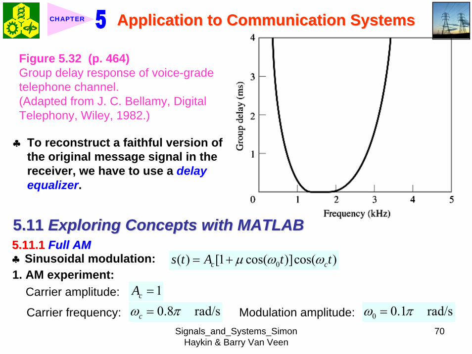
Signals_and_Systems_Simon Haykin amp Barry Van Veen
71
Application to Communication SystemsApplication to Communication SystemsCHAPTER
2 We wish to display and analyze 10 full cycles of the AM wave corresponding to a total duration of 200 s Choosing a sampling rate 1Ts = 10 Hz we have a total of N = 2000 time samples The frequency band of interest is minus 10 π ≦ ω ≦ 10 π Since the separation between the carrier and either side frequency is equal to the modulation frequency ω0 = 01 π rads we would like to have a frequency resolution ωr = 001π rads To achieve this resolution we require the following number of frequency samples (see Eq (442))
20 2000001
s
r
M ω πω π
ge = =
3 We therefore choose M = 2000 To approximate the Fourier transform of the AM wave s(t) we may use a 2000-point DTFS The only variable in the AM experiment is the modulation factor μ with respect to which we wish to investigate three different situationsμ = 05 corresponding to under-modulationμ = 10 for which the AM system is on the verge of over-modulationμ = 20 corresponding to over-modulation
Signals_and_Systems_Simon Haykin amp Barry Van Veen
72
Application to Communication SystemsApplication to Communication SystemsCHAPTER
4 MATLAB commandsAc = 1 carrier amplitudewc = 08pi carrier frequencyw0 = 01pi modulation frequencymu = 05 modulation factort = 0011999s = Ac(1 + mucos(w0t))cos(wct)plot(ts)Smag = abs(fftshift(fft(s2000)))2000 Smag denotes the magnitude specturm of the AM wavew = 10[-1000999]2pi2000plot(wSmag)axis ([-30 30 0 08])
5 5 μμ = 05 = 05 case case Fig 533Fig 533μμ = 10 case = 10 case Fig 534Fig 534μμ = 20 case = 20 case Fig 535Fig 535
Discussion see pp 466-469 textbook
Signals_and_Systems_Simon Haykin amp Barry Van Veen
73
Application to Communication SystemsApplication to Communication SystemsCHAPTER
-30 -20 -10 0 10 20 300
02
04
06
0 50 100 150 200-2
-1
0
1
2
2 22 24 26 28 3
02
04
06
(a) Time (s)
Time domain
Frequency domain
(b) Frequency (rads)
Frequency domain
Frequency (rads)
Figure 533 (p 466)Amplitude modulation with 50 modulation (a) AM wave (b) magnitude spectrum of the AM wave and (c) expanded spectrum around the carrier frequency
μμ = 05 = 05 casecase
Signals_and_Systems_Simon Haykin amp Barry Van Veen
74
Application to Communication SystemsApplication to Communication SystemsCHAPTER
Figure 534 (p 467)Figure 534 (p 467)Amplitude modulation with 100 modulation (a) AM wave (b) magnitude spectrum of the AM wave and (c) expanded spectrum around the carrier frequency
Signals_and_Systems_Simon Haykin amp Barry Van Veen
75
Application to Communication SystemsApplication to Communication SystemsCHAPTER
Figure 535 (p 468)Amplitude modulation with 200 modulation (a) AM wave (b) magnitude spectrum of the AM wave and (c) expanded spectrum around the carrier frequency
Signals_and_Systems_Simon Haykin amp Barry Van Veen
76
Application to Communication SystemsApplication to Communication SystemsCHAPTER
5112 5112 DSBDSB--SC ModulationSC Modulation1 Sinusoidal modulation
0 0( ) cos( ) cos( )c cs t A A t tω ω=
2 MATLAB commands
Ac = 1 carrier amplitudewc = 08pi carrier frequency in radsA0 = 1 amplitude of modulating signalw0 = 01pi frequency of modulating signalt = 011999s = AcA0cos(wct)cos(w0t)plot(ts)Smag = abs(fftshift(fft(s2000)))2000w = 10[-1000999]2pi2000plot(wSmag)
3 3 DSBDSB--SC modulated waveSC modulated wave Fig 536Fig 536 Discussion see pp 466-469 textbook
4 Output of the product modulator in Fig 512 (b) with φ = 0
Signals_and_Systems_Simon Haykin amp Barry Van Veen
77
Application to Communication SystemsApplication to Communication SystemsCHAPTER
Figure 536 (p 469)DSB-SC modulation (a) DSB-SC modulated wave (b) magnitude spectrum of the modulated wave and (c) expanded spectrum around the carrier frequency
Signals_and_Systems_Simon Haykin amp Barry Van Veen
78
Application to Communication SystemsApplication to Communication SystemsCHAPTER
( ) ( ) cos( )cv t s t tω=
5 MATLAB commandsgtgt v = scos(wct)
6 Fig 537 (a) waveforms of v(t) Fig 537 (b) magnitude spectrum which readily shows that v(t) consists of the following components1) A sinusoidal component with frequency 01π rads representing the
modulating wave2) A new DSB-SC modulated wave with double carrier frequency of 16π rads
in actuality the side frequencies of this modulated wave are located at 15πand 17π rads
1) The frequency of the modulating wave lies inside the passband of the filter2) The upper and lower side frequencies of the new DSB-SC modulated wave
lie inside the stopband of the filter
Accordingly we may recover the sinusoidal modulating signal by passing v(t) through low-pass filter with the following requirements
Signals_and_Systems_Simon Haykin amp Barry Van Veen
79
Application to Communication SystemsApplication to Communication SystemsCHAPTER
Figure 537 (p 470)Coherent detection of DSB-SC modulated wave (a) and (b) Waveform and magnitude spectrum of signal produced at the output of produce modulator (c) and (d) waveform and magnitude spectrum of low-pass filter output
Signals_and_Systems_Simon Haykin amp Barry Van Veen
80
Application to Communication SystemsApplication to Communication SystemsCHAPTER
The issue of how to design a filter with these requirements will be considered in detail in Chapter 8 For the present it suffices to say that the preceding requirements can be met by using the following MATLAB commands
gtgt [ba] = butter(30025)gtgt output = filter(bav)
The first command produces s special type of filter called a Butterworth filter For the experiment considered here the filter order is 3 and its normalized cutoff frequency of 0025 is calculated as follows
Actual cutoff frequency of filter 025 radsHalf the sampling rate 10 rads
0025
ππ
=
=
The second command computes the filterrsquos output in response to the product modulator output v(t) (We will revisit the design of this filter in Chapter 8) Figure 537(c) displays the waveform of the low-pass filter output this waveform represents a sinusoidal signal of frequency 005 Hz an observation that is confirmed by using the ffr command to approximate the spectrum of the filter output The result of the computation is shown in Fig 537(d)Fig 537(d)
Signals_and_Systems_Simon Haykin amp Barry Van Veen
81
Application to Communication SystemsApplication to Communication SystemsCHAPTER
7 In Fig 538 we explore another aspect of DSB-SC modulation namely the effect of varying the modulation frequency Figure 538(a) shows five cycles of a DSB-SC modulated wave that has the same carrier frequency as that in Fig 536(a) but the modulation frequency has been reduced to 0025 Hz( ie a radian frequency of 005π) Figure 538(b) shows the magnitude spectrum of this second DSB-SC modulated wave and its zoomed-in version is shown in Fig 538(c) Comparing this latter figure with Fig 536(c) we see clearly that decreasing the modulation frequency has the effect of moving the upper and lower side frequencies closer together which is consistent with modulation theory
5113 5113 Phase and Group DelayPhase and Group Delay1 In Example 58 we studied the phase and group delays for a band-pass
channel with phase response 2 2
1( ) tan c
c
ω ωφ ωωω
minus ⎛ ⎞minus= minus ⎜ ⎟
⎝ ⎠2 At ω = ωc the phase delay is τ p = 0 and the group delay is τ s = 04211s One
of the wave forms displayed in Fig 531Fig 531 is
1( ) ( ) cos( )cx t s t tω=
Signals_and_Systems_Simon Haykin amp Barry Van Veen
82
Application to Communication SystemsApplication to Communication SystemsCHAPTER
Figure 538 (p 472)Effect of varying the modulation frequency compared with that in Fig 537 (a) and (b) Waveform and magnitude spectrum of DSB-SC modulated wave with a modulation frequency one-half that used in Fig 536 (c) expanded spectrum around the carrier frequency
Signals_and_Systems_Simon Haykin amp Barry Van Veen
83
Application to Communication SystemsApplication to Communication SystemsCHAPTER
where (see page 461)
1 2( ) [cos( ) cos( )]2As t t tω ω= +
and ω1 = ωc + ω0 and ω2 = ωc - ω0 The waveform shown in the figure as a solid curve is a plot of x1(t) The other waveform also displayed in Fig 531Fig 531 is
2
1 1 2 2
( ) ( ) cos( )
[cos( ( )) cos( ( ))]cos( )2
c
c
x t y t tA t t t
ω
ω φ ω ω φ ω ω
=
= + + +
where the angle φ (ω1) and φ (ω2) are the values of the phase response φ (ω) at ω = ω1 and ω = ω2 respectively The waveform shown as a dotted curve in the figure is a plot of x2(t)
3 The generation of x1(t) and x2(t) in MATLAB is achieved with the following commands with A2 set equal to unity
Signals_and_Systems_Simon Haykin amp Barry Van Veen
84
Application to Communication SystemsApplication to Communication SystemsCHAPTER
wc = 475w0 = 025w1 = wc + w0w2 = wc - w0t = -10 0001 10o1 = -atan((w1^2 - wc^2)(w1wc))o2 = -atan((w2^2 - wc^2)(w2wc))s = cos(w1t) + cos(w2t)y = cos(w1t + o1) + cos(w2t + o2)x1 = scos(478t)x2 = ycos(475t)plot(tx1b)hold on plot(tx2k)hold offxlabel(Time)ylabel(Amplitude)
Note that we have set (A2) = 1 for convenience of presentation The function atan in the first two commands returns the arctangent Note also that the computation of both x1 and x2 involve element-by-element multiplications ndash hence the use of period followed by an asterisk
Signals_and_Systems_Simon Haykin amp Barry Van Veen
85
Application to Communication SystemsApplication to Communication SystemsCHAPTER
Signals_and_Systems_Simon Haykin amp Barry Van Veen
86
Application to Communication SystemsApplication to Communication SystemsCHAPTER
Signals_and_Systems_Simon Haykin amp Barry Van Veen
87
Application to Communication SystemsApplication to Communication SystemsCHAPTER
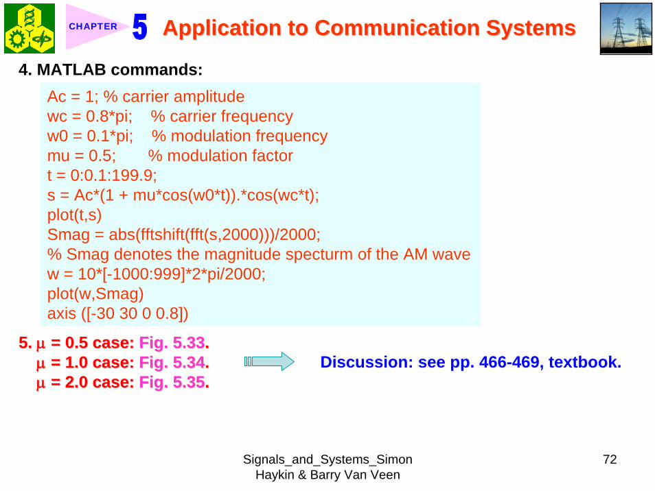
Signals_and_Systems_Simon Haykin amp Barry Van Veen
73
Application to Communication SystemsApplication to Communication SystemsCHAPTER
-30 -20 -10 0 10 20 300
02
04
06
0 50 100 150 200-2
-1
0
1
2
2 22 24 26 28 3
02
04
06
(a) Time (s)
Time domain
Frequency domain
(b) Frequency (rads)
Frequency domain
Frequency (rads)
Figure 533 (p 466)Amplitude modulation with 50 modulation (a) AM wave (b) magnitude spectrum of the AM wave and (c) expanded spectrum around the carrier frequency
μμ = 05 = 05 casecase
Signals_and_Systems_Simon Haykin amp Barry Van Veen
74
Application to Communication SystemsApplication to Communication SystemsCHAPTER
Figure 534 (p 467)Figure 534 (p 467)Amplitude modulation with 100 modulation (a) AM wave (b) magnitude spectrum of the AM wave and (c) expanded spectrum around the carrier frequency
Signals_and_Systems_Simon Haykin amp Barry Van Veen
75
Application to Communication SystemsApplication to Communication SystemsCHAPTER
Figure 535 (p 468)Amplitude modulation with 200 modulation (a) AM wave (b) magnitude spectrum of the AM wave and (c) expanded spectrum around the carrier frequency
Signals_and_Systems_Simon Haykin amp Barry Van Veen
76
Application to Communication SystemsApplication to Communication SystemsCHAPTER
5112 5112 DSBDSB--SC ModulationSC Modulation1 Sinusoidal modulation
0 0( ) cos( ) cos( )c cs t A A t tω ω=
2 MATLAB commands
Ac = 1 carrier amplitudewc = 08pi carrier frequency in radsA0 = 1 amplitude of modulating signalw0 = 01pi frequency of modulating signalt = 011999s = AcA0cos(wct)cos(w0t)plot(ts)Smag = abs(fftshift(fft(s2000)))2000w = 10[-1000999]2pi2000plot(wSmag)
3 3 DSBDSB--SC modulated waveSC modulated wave Fig 536Fig 536 Discussion see pp 466-469 textbook
4 Output of the product modulator in Fig 512 (b) with φ = 0
Signals_and_Systems_Simon Haykin amp Barry Van Veen
77
Application to Communication SystemsApplication to Communication SystemsCHAPTER
Figure 536 (p 469)DSB-SC modulation (a) DSB-SC modulated wave (b) magnitude spectrum of the modulated wave and (c) expanded spectrum around the carrier frequency
Signals_and_Systems_Simon Haykin amp Barry Van Veen
78
Application to Communication SystemsApplication to Communication SystemsCHAPTER
( ) ( ) cos( )cv t s t tω=
5 MATLAB commandsgtgt v = scos(wct)
6 Fig 537 (a) waveforms of v(t) Fig 537 (b) magnitude spectrum which readily shows that v(t) consists of the following components1) A sinusoidal component with frequency 01π rads representing the
modulating wave2) A new DSB-SC modulated wave with double carrier frequency of 16π rads
in actuality the side frequencies of this modulated wave are located at 15πand 17π rads
1) The frequency of the modulating wave lies inside the passband of the filter2) The upper and lower side frequencies of the new DSB-SC modulated wave
lie inside the stopband of the filter
Accordingly we may recover the sinusoidal modulating signal by passing v(t) through low-pass filter with the following requirements
Signals_and_Systems_Simon Haykin amp Barry Van Veen
79
Application to Communication SystemsApplication to Communication SystemsCHAPTER
Figure 537 (p 470)Coherent detection of DSB-SC modulated wave (a) and (b) Waveform and magnitude spectrum of signal produced at the output of produce modulator (c) and (d) waveform and magnitude spectrum of low-pass filter output
Signals_and_Systems_Simon Haykin amp Barry Van Veen
80
Application to Communication SystemsApplication to Communication SystemsCHAPTER
The issue of how to design a filter with these requirements will be considered in detail in Chapter 8 For the present it suffices to say that the preceding requirements can be met by using the following MATLAB commands
gtgt [ba] = butter(30025)gtgt output = filter(bav)
The first command produces s special type of filter called a Butterworth filter For the experiment considered here the filter order is 3 and its normalized cutoff frequency of 0025 is calculated as follows
Actual cutoff frequency of filter 025 radsHalf the sampling rate 10 rads
0025
ππ
=
=
The second command computes the filterrsquos output in response to the product modulator output v(t) (We will revisit the design of this filter in Chapter 8) Figure 537(c) displays the waveform of the low-pass filter output this waveform represents a sinusoidal signal of frequency 005 Hz an observation that is confirmed by using the ffr command to approximate the spectrum of the filter output The result of the computation is shown in Fig 537(d)Fig 537(d)
Signals_and_Systems_Simon Haykin amp Barry Van Veen
81
Application to Communication SystemsApplication to Communication SystemsCHAPTER
7 In Fig 538 we explore another aspect of DSB-SC modulation namely the effect of varying the modulation frequency Figure 538(a) shows five cycles of a DSB-SC modulated wave that has the same carrier frequency as that in Fig 536(a) but the modulation frequency has been reduced to 0025 Hz( ie a radian frequency of 005π) Figure 538(b) shows the magnitude spectrum of this second DSB-SC modulated wave and its zoomed-in version is shown in Fig 538(c) Comparing this latter figure with Fig 536(c) we see clearly that decreasing the modulation frequency has the effect of moving the upper and lower side frequencies closer together which is consistent with modulation theory
5113 5113 Phase and Group DelayPhase and Group Delay1 In Example 58 we studied the phase and group delays for a band-pass
channel with phase response 2 2
1( ) tan c
c
ω ωφ ωωω
minus ⎛ ⎞minus= minus ⎜ ⎟
⎝ ⎠2 At ω = ωc the phase delay is τ p = 0 and the group delay is τ s = 04211s One
of the wave forms displayed in Fig 531Fig 531 is
1( ) ( ) cos( )cx t s t tω=
Signals_and_Systems_Simon Haykin amp Barry Van Veen
82
Application to Communication SystemsApplication to Communication SystemsCHAPTER
Figure 538 (p 472)Effect of varying the modulation frequency compared with that in Fig 537 (a) and (b) Waveform and magnitude spectrum of DSB-SC modulated wave with a modulation frequency one-half that used in Fig 536 (c) expanded spectrum around the carrier frequency
Signals_and_Systems_Simon Haykin amp Barry Van Veen
83
Application to Communication SystemsApplication to Communication SystemsCHAPTER
where (see page 461)
1 2( ) [cos( ) cos( )]2As t t tω ω= +
and ω1 = ωc + ω0 and ω2 = ωc - ω0 The waveform shown in the figure as a solid curve is a plot of x1(t) The other waveform also displayed in Fig 531Fig 531 is
2
1 1 2 2
( ) ( ) cos( )
[cos( ( )) cos( ( ))]cos( )2
c
c
x t y t tA t t t
ω
ω φ ω ω φ ω ω
=
= + + +
where the angle φ (ω1) and φ (ω2) are the values of the phase response φ (ω) at ω = ω1 and ω = ω2 respectively The waveform shown as a dotted curve in the figure is a plot of x2(t)
3 The generation of x1(t) and x2(t) in MATLAB is achieved with the following commands with A2 set equal to unity
Signals_and_Systems_Simon Haykin amp Barry Van Veen
84
Application to Communication SystemsApplication to Communication SystemsCHAPTER
wc = 475w0 = 025w1 = wc + w0w2 = wc - w0t = -10 0001 10o1 = -atan((w1^2 - wc^2)(w1wc))o2 = -atan((w2^2 - wc^2)(w2wc))s = cos(w1t) + cos(w2t)y = cos(w1t + o1) + cos(w2t + o2)x1 = scos(478t)x2 = ycos(475t)plot(tx1b)hold on plot(tx2k)hold offxlabel(Time)ylabel(Amplitude)
Note that we have set (A2) = 1 for convenience of presentation The function atan in the first two commands returns the arctangent Note also that the computation of both x1 and x2 involve element-by-element multiplications ndash hence the use of period followed by an asterisk
Signals_and_Systems_Simon Haykin amp Barry Van Veen
85
Application to Communication SystemsApplication to Communication SystemsCHAPTER
Signals_and_Systems_Simon Haykin amp Barry Van Veen
86
Application to Communication SystemsApplication to Communication SystemsCHAPTER
Signals_and_Systems_Simon Haykin amp Barry Van Veen
87
Application to Communication SystemsApplication to Communication SystemsCHAPTER
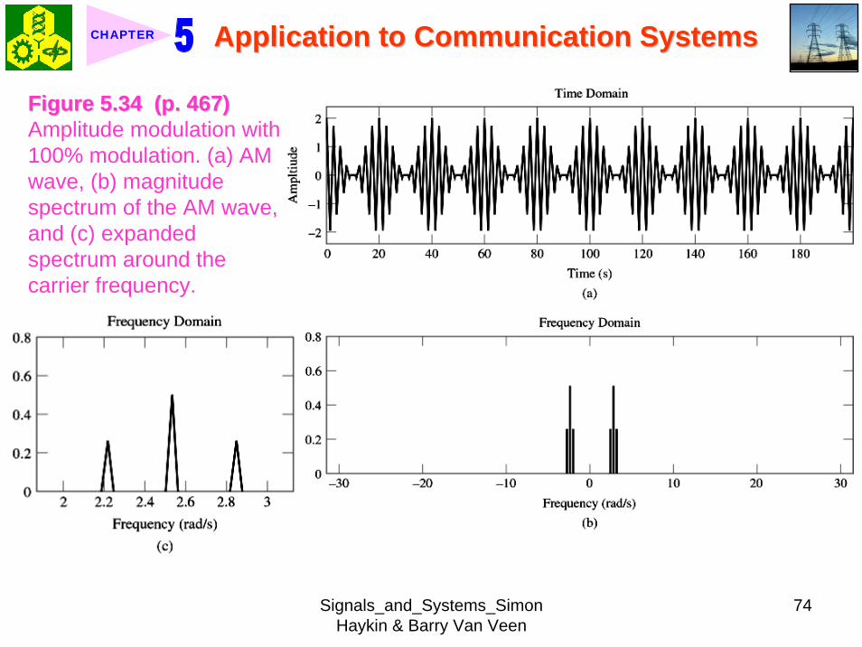
Signals_and_Systems_Simon Haykin amp Barry Van Veen
78
Application to Communication SystemsApplication to Communication SystemsCHAPTER
( ) ( ) cos( )cv t s t tω=
5 MATLAB commandsgtgt v = scos(wct)
6 Fig 537 (a) waveforms of v(t) Fig 537 (b) magnitude spectrum which readily shows that v(t) consists of the following components1) A sinusoidal component with frequency 01π rads representing the
modulating wave2) A new DSB-SC modulated wave with double carrier frequency of 16π rads
in actuality the side frequencies of this modulated wave are located at 15πand 17π rads
1) The frequency of the modulating wave lies inside the passband of the filter2) The upper and lower side frequencies of the new DSB-SC modulated wave
lie inside the stopband of the filter
Accordingly we may recover the sinusoidal modulating signal by passing v(t) through low-pass filter with the following requirements
Signals_and_Systems_Simon Haykin amp Barry Van Veen
79
Application to Communication SystemsApplication to Communication SystemsCHAPTER
Figure 537 (p 470)Coherent detection of DSB-SC modulated wave (a) and (b) Waveform and magnitude spectrum of signal produced at the output of produce modulator (c) and (d) waveform and magnitude spectrum of low-pass filter output
Signals_and_Systems_Simon Haykin amp Barry Van Veen
80
Application to Communication SystemsApplication to Communication SystemsCHAPTER
The issue of how to design a filter with these requirements will be considered in detail in Chapter 8 For the present it suffices to say that the preceding requirements can be met by using the following MATLAB commands
gtgt [ba] = butter(30025)gtgt output = filter(bav)
The first command produces s special type of filter called a Butterworth filter For the experiment considered here the filter order is 3 and its normalized cutoff frequency of 0025 is calculated as follows
Actual cutoff frequency of filter 025 radsHalf the sampling rate 10 rads
0025
ππ
=
=
The second command computes the filterrsquos output in response to the product modulator output v(t) (We will revisit the design of this filter in Chapter 8) Figure 537(c) displays the waveform of the low-pass filter output this waveform represents a sinusoidal signal of frequency 005 Hz an observation that is confirmed by using the ffr command to approximate the spectrum of the filter output The result of the computation is shown in Fig 537(d)Fig 537(d)
Signals_and_Systems_Simon Haykin amp Barry Van Veen
81
Application to Communication SystemsApplication to Communication SystemsCHAPTER
7 In Fig 538 we explore another aspect of DSB-SC modulation namely the effect of varying the modulation frequency Figure 538(a) shows five cycles of a DSB-SC modulated wave that has the same carrier frequency as that in Fig 536(a) but the modulation frequency has been reduced to 0025 Hz( ie a radian frequency of 005π) Figure 538(b) shows the magnitude spectrum of this second DSB-SC modulated wave and its zoomed-in version is shown in Fig 538(c) Comparing this latter figure with Fig 536(c) we see clearly that decreasing the modulation frequency has the effect of moving the upper and lower side frequencies closer together which is consistent with modulation theory
5113 5113 Phase and Group DelayPhase and Group Delay1 In Example 58 we studied the phase and group delays for a band-pass
channel with phase response 2 2
1( ) tan c
c
ω ωφ ωωω
minus ⎛ ⎞minus= minus ⎜ ⎟
⎝ ⎠2 At ω = ωc the phase delay is τ p = 0 and the group delay is τ s = 04211s One
of the wave forms displayed in Fig 531Fig 531 is
1( ) ( ) cos( )cx t s t tω=
Signals_and_Systems_Simon Haykin amp Barry Van Veen
82
Application to Communication SystemsApplication to Communication SystemsCHAPTER
Figure 538 (p 472)Effect of varying the modulation frequency compared with that in Fig 537 (a) and (b) Waveform and magnitude spectrum of DSB-SC modulated wave with a modulation frequency one-half that used in Fig 536 (c) expanded spectrum around the carrier frequency
Signals_and_Systems_Simon Haykin amp Barry Van Veen
83
Application to Communication SystemsApplication to Communication SystemsCHAPTER
where (see page 461)
1 2( ) [cos( ) cos( )]2As t t tω ω= +
and ω1 = ωc + ω0 and ω2 = ωc - ω0 The waveform shown in the figure as a solid curve is a plot of x1(t) The other waveform also displayed in Fig 531Fig 531 is
2
1 1 2 2
( ) ( ) cos( )
[cos( ( )) cos( ( ))]cos( )2
c
c
x t y t tA t t t
ω
ω φ ω ω φ ω ω
=
= + + +
where the angle φ (ω1) and φ (ω2) are the values of the phase response φ (ω) at ω = ω1 and ω = ω2 respectively The waveform shown as a dotted curve in the figure is a plot of x2(t)
3 The generation of x1(t) and x2(t) in MATLAB is achieved with the following commands with A2 set equal to unity
Signals_and_Systems_Simon Haykin amp Barry Van Veen
84
Application to Communication SystemsApplication to Communication SystemsCHAPTER
wc = 475w0 = 025w1 = wc + w0w2 = wc - w0t = -10 0001 10o1 = -atan((w1^2 - wc^2)(w1wc))o2 = -atan((w2^2 - wc^2)(w2wc))s = cos(w1t) + cos(w2t)y = cos(w1t + o1) + cos(w2t + o2)x1 = scos(478t)x2 = ycos(475t)plot(tx1b)hold on plot(tx2k)hold offxlabel(Time)ylabel(Amplitude)
Note that we have set (A2) = 1 for convenience of presentation The function atan in the first two commands returns the arctangent Note also that the computation of both x1 and x2 involve element-by-element multiplications ndash hence the use of period followed by an asterisk
Signals_and_Systems_Simon Haykin amp Barry Van Veen
85
Application to Communication SystemsApplication to Communication SystemsCHAPTER
Signals_and_Systems_Simon Haykin amp Barry Van Veen
86
Application to Communication SystemsApplication to Communication SystemsCHAPTER
Signals_and_Systems_Simon Haykin amp Barry Van Veen
87
Application to Communication SystemsApplication to Communication SystemsCHAPTER
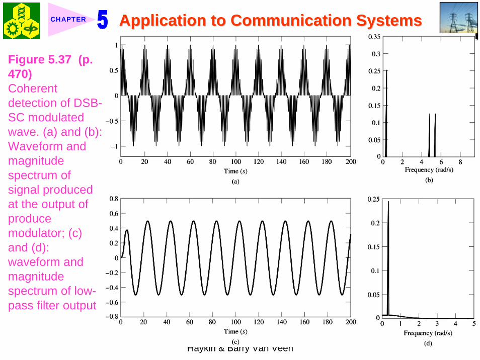
Signals_and_Systems_Simon Haykin amp Barry Van Veen
79
Application to Communication SystemsApplication to Communication SystemsCHAPTER
Figure 537 (p 470)Coherent detection of DSB-SC modulated wave (a) and (b) Waveform and magnitude spectrum of signal produced at the output of produce modulator (c) and (d) waveform and magnitude spectrum of low-pass filter output
Signals_and_Systems_Simon Haykin amp Barry Van Veen
80
Application to Communication SystemsApplication to Communication SystemsCHAPTER
The issue of how to design a filter with these requirements will be considered in detail in Chapter 8 For the present it suffices to say that the preceding requirements can be met by using the following MATLAB commands
gtgt [ba] = butter(30025)gtgt output = filter(bav)
The first command produces s special type of filter called a Butterworth filter For the experiment considered here the filter order is 3 and its normalized cutoff frequency of 0025 is calculated as follows
Actual cutoff frequency of filter 025 radsHalf the sampling rate 10 rads
0025
ππ
=
=
The second command computes the filterrsquos output in response to the product modulator output v(t) (We will revisit the design of this filter in Chapter 8) Figure 537(c) displays the waveform of the low-pass filter output this waveform represents a sinusoidal signal of frequency 005 Hz an observation that is confirmed by using the ffr command to approximate the spectrum of the filter output The result of the computation is shown in Fig 537(d)Fig 537(d)
Signals_and_Systems_Simon Haykin amp Barry Van Veen
81
Application to Communication SystemsApplication to Communication SystemsCHAPTER
7 In Fig 538 we explore another aspect of DSB-SC modulation namely the effect of varying the modulation frequency Figure 538(a) shows five cycles of a DSB-SC modulated wave that has the same carrier frequency as that in Fig 536(a) but the modulation frequency has been reduced to 0025 Hz( ie a radian frequency of 005π) Figure 538(b) shows the magnitude spectrum of this second DSB-SC modulated wave and its zoomed-in version is shown in Fig 538(c) Comparing this latter figure with Fig 536(c) we see clearly that decreasing the modulation frequency has the effect of moving the upper and lower side frequencies closer together which is consistent with modulation theory
5113 5113 Phase and Group DelayPhase and Group Delay1 In Example 58 we studied the phase and group delays for a band-pass
channel with phase response 2 2
1( ) tan c
c
ω ωφ ωωω
minus ⎛ ⎞minus= minus ⎜ ⎟
⎝ ⎠2 At ω = ωc the phase delay is τ p = 0 and the group delay is τ s = 04211s One
of the wave forms displayed in Fig 531Fig 531 is
1( ) ( ) cos( )cx t s t tω=
Signals_and_Systems_Simon Haykin amp Barry Van Veen
82
Application to Communication SystemsApplication to Communication SystemsCHAPTER
Figure 538 (p 472)Effect of varying the modulation frequency compared with that in Fig 537 (a) and (b) Waveform and magnitude spectrum of DSB-SC modulated wave with a modulation frequency one-half that used in Fig 536 (c) expanded spectrum around the carrier frequency
Signals_and_Systems_Simon Haykin amp Barry Van Veen
83
Application to Communication SystemsApplication to Communication SystemsCHAPTER
where (see page 461)
1 2( ) [cos( ) cos( )]2As t t tω ω= +
and ω1 = ωc + ω0 and ω2 = ωc - ω0 The waveform shown in the figure as a solid curve is a plot of x1(t) The other waveform also displayed in Fig 531Fig 531 is
2
1 1 2 2
( ) ( ) cos( )
[cos( ( )) cos( ( ))]cos( )2
c
c
x t y t tA t t t
ω
ω φ ω ω φ ω ω
=
= + + +
where the angle φ (ω1) and φ (ω2) are the values of the phase response φ (ω) at ω = ω1 and ω = ω2 respectively The waveform shown as a dotted curve in the figure is a plot of x2(t)
3 The generation of x1(t) and x2(t) in MATLAB is achieved with the following commands with A2 set equal to unity
Signals_and_Systems_Simon Haykin amp Barry Van Veen
84
Application to Communication SystemsApplication to Communication SystemsCHAPTER
wc = 475w0 = 025w1 = wc + w0w2 = wc - w0t = -10 0001 10o1 = -atan((w1^2 - wc^2)(w1wc))o2 = -atan((w2^2 - wc^2)(w2wc))s = cos(w1t) + cos(w2t)y = cos(w1t + o1) + cos(w2t + o2)x1 = scos(478t)x2 = ycos(475t)plot(tx1b)hold on plot(tx2k)hold offxlabel(Time)ylabel(Amplitude)
Note that we have set (A2) = 1 for convenience of presentation The function atan in the first two commands returns the arctangent Note also that the computation of both x1 and x2 involve element-by-element multiplications ndash hence the use of period followed by an asterisk
Signals_and_Systems_Simon Haykin amp Barry Van Veen
85
Application to Communication SystemsApplication to Communication SystemsCHAPTER
Signals_and_Systems_Simon Haykin amp Barry Van Veen
86
Application to Communication SystemsApplication to Communication SystemsCHAPTER
Signals_and_Systems_Simon Haykin amp Barry Van Veen
87
Application to Communication SystemsApplication to Communication SystemsCHAPTER
Signals_and_Systems_Simon Haykin amp Barry Van Veen
81
Application to Communication SystemsApplication to Communication SystemsCHAPTER
7 In Fig 538 we explore another aspect of DSB-SC modulation namely the effect of varying the modulation frequency Figure 538(a) shows five cycles of a DSB-SC modulated wave that has the same carrier frequency as that in Fig 536(a) but the modulation frequency has been reduced to 0025 Hz( ie a radian frequency of 005π) Figure 538(b) shows the magnitude spectrum of this second DSB-SC modulated wave and its zoomed-in version is shown in Fig 538(c) Comparing this latter figure with Fig 536(c) we see clearly that decreasing the modulation frequency has the effect of moving the upper and lower side frequencies closer together which is consistent with modulation theory
5113 5113 Phase and Group DelayPhase and Group Delay1 In Example 58 we studied the phase and group delays for a band-pass
channel with phase response 2 2
1( ) tan c
c
ω ωφ ωωω
minus ⎛ ⎞minus= minus ⎜ ⎟
⎝ ⎠2 At ω = ωc the phase delay is τ p = 0 and the group delay is τ s = 04211s One
of the wave forms displayed in Fig 531Fig 531 is
1( ) ( ) cos( )cx t s t tω=
Signals_and_Systems_Simon Haykin amp Barry Van Veen
82
Application to Communication SystemsApplication to Communication SystemsCHAPTER
Figure 538 (p 472)Effect of varying the modulation frequency compared with that in Fig 537 (a) and (b) Waveform and magnitude spectrum of DSB-SC modulated wave with a modulation frequency one-half that used in Fig 536 (c) expanded spectrum around the carrier frequency
Signals_and_Systems_Simon Haykin amp Barry Van Veen
83
Application to Communication SystemsApplication to Communication SystemsCHAPTER
where (see page 461)
1 2( ) [cos( ) cos( )]2As t t tω ω= +
and ω1 = ωc + ω0 and ω2 = ωc - ω0 The waveform shown in the figure as a solid curve is a plot of x1(t) The other waveform also displayed in Fig 531Fig 531 is
2
1 1 2 2
( ) ( ) cos( )
[cos( ( )) cos( ( ))]cos( )2
c
c
x t y t tA t t t
ω
ω φ ω ω φ ω ω
=
= + + +
where the angle φ (ω1) and φ (ω2) are the values of the phase response φ (ω) at ω = ω1 and ω = ω2 respectively The waveform shown as a dotted curve in the figure is a plot of x2(t)
3 The generation of x1(t) and x2(t) in MATLAB is achieved with the following commands with A2 set equal to unity
Signals_and_Systems_Simon Haykin amp Barry Van Veen
84
Application to Communication SystemsApplication to Communication SystemsCHAPTER
wc = 475w0 = 025w1 = wc + w0w2 = wc - w0t = -10 0001 10o1 = -atan((w1^2 - wc^2)(w1wc))o2 = -atan((w2^2 - wc^2)(w2wc))s = cos(w1t) + cos(w2t)y = cos(w1t + o1) + cos(w2t + o2)x1 = scos(478t)x2 = ycos(475t)plot(tx1b)hold on plot(tx2k)hold offxlabel(Time)ylabel(Amplitude)
Note that we have set (A2) = 1 for convenience of presentation The function atan in the first two commands returns the arctangent Note also that the computation of both x1 and x2 involve element-by-element multiplications ndash hence the use of period followed by an asterisk
Signals_and_Systems_Simon Haykin amp Barry Van Veen
85
Application to Communication SystemsApplication to Communication SystemsCHAPTER
Signals_and_Systems_Simon Haykin amp Barry Van Veen
86
Application to Communication SystemsApplication to Communication SystemsCHAPTER
Signals_and_Systems_Simon Haykin amp Barry Van Veen
87
Application to Communication SystemsApplication to Communication SystemsCHAPTER
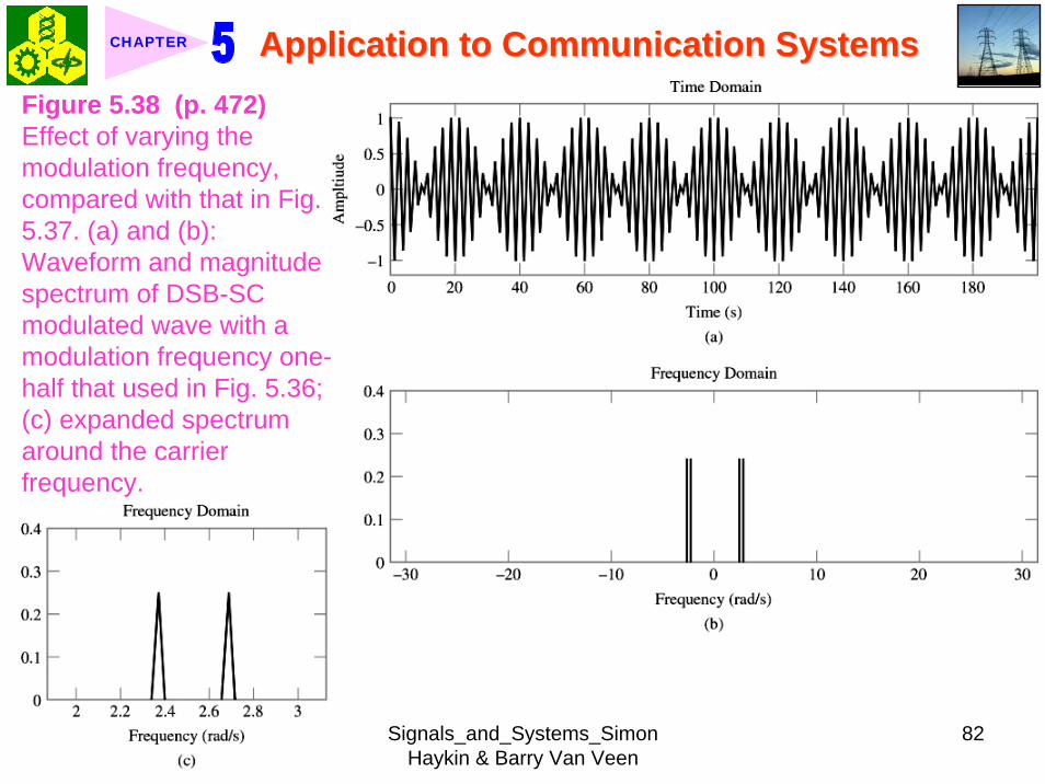
Signals_and_Systems_Simon Haykin amp Barry Van Veen
82
Application to Communication SystemsApplication to Communication SystemsCHAPTER
Figure 538 (p 472)Effect of varying the modulation frequency compared with that in Fig 537 (a) and (b) Waveform and magnitude spectrum of DSB-SC modulated wave with a modulation frequency one-half that used in Fig 536 (c) expanded spectrum around the carrier frequency
Signals_and_Systems_Simon Haykin amp Barry Van Veen
83
Application to Communication SystemsApplication to Communication SystemsCHAPTER
where (see page 461)
1 2( ) [cos( ) cos( )]2As t t tω ω= +
and ω1 = ωc + ω0 and ω2 = ωc - ω0 The waveform shown in the figure as a solid curve is a plot of x1(t) The other waveform also displayed in Fig 531Fig 531 is
2
1 1 2 2
( ) ( ) cos( )
[cos( ( )) cos( ( ))]cos( )2
c
c
x t y t tA t t t
ω
ω φ ω ω φ ω ω
=
= + + +
where the angle φ (ω1) and φ (ω2) are the values of the phase response φ (ω) at ω = ω1 and ω = ω2 respectively The waveform shown as a dotted curve in the figure is a plot of x2(t)
3 The generation of x1(t) and x2(t) in MATLAB is achieved with the following commands with A2 set equal to unity
Signals_and_Systems_Simon Haykin amp Barry Van Veen
84
Application to Communication SystemsApplication to Communication SystemsCHAPTER
wc = 475w0 = 025w1 = wc + w0w2 = wc - w0t = -10 0001 10o1 = -atan((w1^2 - wc^2)(w1wc))o2 = -atan((w2^2 - wc^2)(w2wc))s = cos(w1t) + cos(w2t)y = cos(w1t + o1) + cos(w2t + o2)x1 = scos(478t)x2 = ycos(475t)plot(tx1b)hold on plot(tx2k)hold offxlabel(Time)ylabel(Amplitude)
Note that we have set (A2) = 1 for convenience of presentation The function atan in the first two commands returns the arctangent Note also that the computation of both x1 and x2 involve element-by-element multiplications ndash hence the use of period followed by an asterisk
Signals_and_Systems_Simon Haykin amp Barry Van Veen
85
Application to Communication SystemsApplication to Communication SystemsCHAPTER
Signals_and_Systems_Simon Haykin amp Barry Van Veen
86
Application to Communication SystemsApplication to Communication SystemsCHAPTER
Signals_and_Systems_Simon Haykin amp Barry Van Veen
87
Application to Communication SystemsApplication to Communication SystemsCHAPTER
Signals_and_Systems_Simon Haykin amp Barry Van Veen
83
Application to Communication SystemsApplication to Communication SystemsCHAPTER
where (see page 461)
1 2( ) [cos( ) cos( )]2As t t tω ω= +
and ω1 = ωc + ω0 and ω2 = ωc - ω0 The waveform shown in the figure as a solid curve is a plot of x1(t) The other waveform also displayed in Fig 531Fig 531 is
2
1 1 2 2
( ) ( ) cos( )
[cos( ( )) cos( ( ))]cos( )2
c
c
x t y t tA t t t
ω
ω φ ω ω φ ω ω
=
= + + +
where the angle φ (ω1) and φ (ω2) are the values of the phase response φ (ω) at ω = ω1 and ω = ω2 respectively The waveform shown as a dotted curve in the figure is a plot of x2(t)
3 The generation of x1(t) and x2(t) in MATLAB is achieved with the following commands with A2 set equal to unity
Signals_and_Systems_Simon Haykin amp Barry Van Veen
84
Application to Communication SystemsApplication to Communication SystemsCHAPTER
wc = 475w0 = 025w1 = wc + w0w2 = wc - w0t = -10 0001 10o1 = -atan((w1^2 - wc^2)(w1wc))o2 = -atan((w2^2 - wc^2)(w2wc))s = cos(w1t) + cos(w2t)y = cos(w1t + o1) + cos(w2t + o2)x1 = scos(478t)x2 = ycos(475t)plot(tx1b)hold on plot(tx2k)hold offxlabel(Time)ylabel(Amplitude)
Note that we have set (A2) = 1 for convenience of presentation The function atan in the first two commands returns the arctangent Note also that the computation of both x1 and x2 involve element-by-element multiplications ndash hence the use of period followed by an asterisk
Signals_and_Systems_Simon Haykin amp Barry Van Veen
85
Application to Communication SystemsApplication to Communication SystemsCHAPTER
Signals_and_Systems_Simon Haykin amp Barry Van Veen
86
Application to Communication SystemsApplication to Communication SystemsCHAPTER
Signals_and_Systems_Simon Haykin amp Barry Van Veen
87
Application to Communication SystemsApplication to Communication SystemsCHAPTER

Signals_and_Systems_Simon Haykin amp Barry Van Veen
86
Application to Communication SystemsApplication to Communication SystemsCHAPTER
Signals_and_Systems_Simon Haykin amp Barry Van Veen
87
Application to Communication SystemsApplication to Communication SystemsCHAPTER
Signals_and_Systems_Simon Haykin amp Barry Van Veen
87
Application to Communication SystemsApplication to Communication SystemsCHAPTER

![Signals and Systems [Haykin]](https://static.fdocuments.net/doc/165x107/548c5b82b47959dc3a8b4674/signals-and-systems-haykin.jpg)