
5 Equal-order segregated finite-element method for fluid … · Sunden CH005.tex 10/9/2010 15: 0...
43
5 Equal-order segregated finite-element method for fluid flow and heat transfer simulation Jianhui Xie MFG-Engineering Design & Simulation, Autodesk, Inc., San Rafael, CA, USA Abstract This chapter introduces finite element–based equal-order mixed-GLS (Galerkin Least Squares) segregated formulation for fluid flow and heat transfer. This scheme follows the idea used in finite-volume method, which decouples the fluid pressure calculation and velocity calculation by taking the divergence of the vector momen- tum equation and applying some clear insights regarding incompressible flow. The inherent velocity correction step in “segregated scheme” makes it attractive for solution robustness and much faster compared to original fluid velocity–pressure coupling scheme because mixed-GLS finite-element formulation does not assure the mass conservation between the interface of the elements in comparison to finite- volume method. With these advantages, this formulation has prevailed in recent years in major finite element–based commercial codes used in the industry sim- ulation models that usually import geometry from CAD and have large scale of degree of freedoms to solve. Taking example of fluid–thermal coupling problem, this chapter also discusses the strategies used to solve multiphysics problem in non- linear iteration level and the block I/O technique that uses finite-element method for handling massive data. Finally, this chapter illustrates some typical industry conjugate heat transfer problems where both solid and fluid parts are involved. Keywords: Finite elements, Fluid flow, Heat transfer, Segregated formulation 5.1 Introduction The quest for robust and efficient strategies to solve large, sparse matrix sys- tems has been an active area of research and development for decades. Galerkin finite-element methods, with the advantages of handling irregular geometry and multiphysics coupling, have played an important role in computational fluid dynam- ics area, but its computational difficulties and perceived shortcomings have led to the development of alternative finite-element models. www.witpress.com, ISSN 1755-8336 (on-line) WIT Transactions on State of the Art in Science and Engineering, Vol 41, © 20 WIT Press 10 doi:10.2495/978-1-84564-144-3/05
Transcript of 5 Equal-order segregated finite-element method for fluid … · Sunden CH005.tex 10/9/2010 15: 0...

Sunden CH005.tex 10/9/2010 15: 0 Page 171
5 Equal-order segregated finite-elementmethod for fluid flow and heat transfersimulation
Jianhui XieMFG-Engineering Design & Simulation, Autodesk, Inc.,San Rafael, CA, USA
Abstract
This chapter introduces finite element–based equal-order mixed-GLS (GalerkinLeast Squares) segregated formulation for fluid flow and heat transfer. This schemefollows the idea used in finite-volume method, which decouples the fluid pressurecalculation and velocity calculation by taking the divergence of the vector momen-tum equation and applying some clear insights regarding incompressible flow. Theinherent velocity correction step in “segregated scheme” makes it attractive forsolution robustness and much faster compared to original fluid velocity–pressurecoupling scheme because mixed-GLS finite-element formulation does not assurethe mass conservation between the interface of the elements in comparison to finite-volume method. With these advantages, this formulation has prevailed in recentyears in major finite element–based commercial codes used in the industry sim-ulation models that usually import geometry from CAD and have large scale ofdegree of freedoms to solve. Taking example of fluid–thermal coupling problem,this chapter also discusses the strategies used to solve multiphysics problem in non-linear iteration level and the block I/O technique that uses finite-element methodfor handling massive data. Finally, this chapter illustrates some typical industryconjugate heat transfer problems where both solid and fluid parts are involved.
Keywords: Finite elements, Fluid flow, Heat transfer, Segregated formulation
5.1 Introduction
The quest for robust and efficient strategies to solve large, sparse matrix sys-tems has been an active area of research and development for decades. Galerkinfinite-element methods, with the advantages of handling irregular geometry andmultiphysics coupling, have played an important role in computational fluid dynam-ics area, but its computational difficulties and perceived shortcomings have led tothe development of alternative finite-element models.
www.witpress.com, ISSN 1755-8336 (on-line) WIT Transactions on State of the Art in Science and Engineering, Vol 41, © 20 WIT Press10
doi:10.2495/978-1-84564-144-3/05

Sunden CH005.tex 10/9/2010 15: 0 Page 172
172 Computational Fluid Dynamics and Heat Transfer
Theoretically, the efforts have been to avoid the two major problems encoun-tered. The first problem is the “wiggles” velocity field problem related to thenode-to-node oscillation of velocity components emanating from boundaries withlarge velocity gradient. This problem is mostly pronounced under the condition ofhigh Reynolds numbers and coarse computational mesh, and therefore the inabil-ity of the finite-element mesh to handle the steep gradient results in an imbalancebetween advective and diffusive contribution. With getting best fit to the prob-lem, the weighted residual formulation produces a field that oscillates about thetrue solution (wiggle pattern). The second problem is the “saddle-point” prob-lem originated by mixed Galerkin finite-element formulation. It is difficult tosolve especially in three-dimensional large-scale industry model because the LBB(Ladyzhenskaya–Babuska–Brezzi) stability condition associated with the Galerkinfinite-element limits element choice with respect to the velocity and pressureinterpolation.
In practical aspect, solution schemes/solvers and algorithms have been exploredfor better CFD processor efficiency and robustness, which are mostly addressed bycommercial codes.
In this chapter, the equal-order mixed-GLS (Galerkin Least Squares) stabi-lized formulation is presented first. It is termed as a residual method becausethe added least-squares terms are weighted residuals of the momentum equa-tion, and this form of the least-squares terms implies the consistency of themethod since the momentum residual is employed. And this method is a gen-eralization of SUPG (streamline-upwind/Petrov–Galerkin) and PSPG (pressurestabilizing/Petrov–Galerkin) methods, which were developed to target the wig-gle stabilization. Since this method plays a significant stabilization role for thecoarse mesh and hybrid mesh, the equal-order velocity and pressure interpolationis viable, and the LBB condition is not necessary any more, the convenient bilinearelement interpolation becomes practical approximation although it was unstable inthe Galerkin finite-element context.
The second emphasis in this chapter is on the practical view: The numer-ical strategies for the solution of large systems of equations arising from thefinite-element discretization of the above formulations are discussed. To solve thenonlinear fluid flow and heat transfer problem, particular emphasis is placed on seg-regated scheme (which uses SIMPLE algorithm from the finite-volume method) innonlinear level and iterative methods in linear level. The velocity–pressure cou-pling formulation not only results in a large dimensioned system but also generatesa stiffness matrix radically different from the narrowband type of matrix, which isinefficient to be solved. Segregated scheme was proposed with the idea of decou-pling the pressure calculation and velocity calculation by taking the divergenceof the vector momentum equation and applying some clear insights regardingincompressible flow. The inherent velocity correction step in “segregated scheme”makes it attractive for solution robustness and faster compared to velocity–pressurecoupling scheme because mixed-GLS finite-element formulation does not assurethe mass conservation between the interface of the elements in comparison tofinite-volume method.
www.witpress.com, ISSN 1755-8336 (on-line) WIT Transactions on State of the Art in Science and Engineering, Vol 41, © 20 WIT Press10

Sunden CH005.tex 10/9/2010 15: 0 Page 173
Equal-order segregated finite-element method 173
According to how the primitive variables of velocity–pressure are treated, finite-element methods for solving Navier–Stokes equations can be categorized into threegroups: (a) the velocity–pressure integrated method; (b) the penalty method; and(c) the segregated velocity–pressure method. The velocity–pressure integratedmethod in which the governing equations are treated simultaneously needs rela-tively small number of iterations to achieve convergence, but a large memory andcomputing time. The penalty method requires less memory and less computing timethan the first method, but it needs an additional postprocessor to obtain pressure fieldand satisfies the continuity equation only approximately. Recently, much attentionhas been paid to the segregated velocity–pressure method, where velocity and thecorresponding pressure field are computed alternatively in an iterative sequence.This method takes advantage of SIMPLE algorithm idea from finite-volume worldand uses it in the finite-element world. With the SIMPLE algorithm idea, it needsmuch less memory and execution time, and with the velocity correction step usingcontinuity equation, it even satisfies the continuity equation better than the firstmethod.
The second categorization of finite-element methods can be made accordingto the orders of interpolation functions for the velocity and pressure. They aremixed-order interpolation and equal-order interpolation. The mixed-order schemeattempts to eliminate the tendency to produce checkerboard pressure distributionsby satisfying LBB condition. In this method the velocity is interpolated linearlywhereas the pressure is assumed to be constant within the element. Equal-orderinterpolation was proposed by Rice and Schnipke [6]. They showed that equal-order scheme performed better for that purpose without exhibiting spurious pressuremodes.
A third categorization of the finite-element method for fluid dynamics isrelated to weight functions. Galerkin method has been widely used in discretiz-ing the momentum equation. Brook and Hughes demonstrated the accuracy ofthe streamline-upwind/Petrov–Galerkin method for the linear advection-diffusionequation; Rice and Schnipke [5] adopted a monotone streamline-upwind finite-element method, where they discretized the momentum equation by using con-vectional Galerkin method with the exception of the advection items, which weretreated by the monotone streamline-upwind approach.
Followed by the success of the finite-volume methods, several finite-elementsegregated solution schemes have been proposed. Rice and Schnipke [6] employedequal-order interpolation for all variables and solved pressure directly; however,their original formulation used a streamline unwinding scheme that may not bestraightforward enough to extend to three-dimensional flows. Early equal-ordermethods were in general of transient kind and the equations had to be integrated ontime to reach a steady state. Van Zijl [11] adapted the formulation by applying SUPGweighting functions to the convective terms; he later adapted the scheme furtherby implementing SIMPLEST algorithm. Shaw [7] demonstrated the way to useelement matrix construction for equal-order interpolation in segregated scheme.Haroutunian et al. [2] have shown that the implementation of iterative solverscan result in a substantial reduction in the storage requirements and execution
www.witpress.com, ISSN 1755-8336 (on-line) WIT Transactions on State of the Art in Science and Engineering, Vol 41, © 20 WIT Press10

Sunden CH005.tex 10/9/2010 15: 0 Page 174
174 Computational Fluid Dynamics and Heat Transfer
time. Du Toit [10] tried conjugate gradient solver; Wang [13,14] demonstrated a“consistent equal-order discretization method” by introducing element-based nodevelocity to satisfy mass conservation, while keeping conventional node velocityand temperature to satisfy momentum and energy equations. Wansophark [15]evaluated segregated schemes by combining monotone streamline-upwind methodand adaptive meshing technique. However, relaxation factors, which need user’sinterpretation, have remained an issue that affects the users.
The classical mixed velocity–pressure interpolation Galerkin finite-elementmethod, often referred to as “mixed v–p form,” was the workhorse of incom-pressible flow solvers in the 1970s to 1990s and has proved highly successful fortwo-dimensional and small three-dimensional problems, offering high order ofaccuracy and strong convergence rates [5]. The high mark of this approach is thediscretization of the continuity equation in a manner adherent to certain mathe-matical constraints, and the ability to simultaneously solve the equation with thediscretized momentum equations in either a Picard or a Newton–Raphson iterativescheme. The discretized continuity equation is the known cause of “indefiniteness”in the resulting Jacobian matrix, leading to unbounded large and negative eigenval-ues. Despite this poor matrix conditioning, most two-dimensional problems withsmall bandwidth are amenable to efficient solution with optimized variations ofclassical Gaussian elimination. For example, skyline method allows for memory-efficient solution and in fact is still used today. But even tremendous technologicaladvances in computer processor speed and random access memory capacity willnever make direct methods a viable alternative for large three-dimensional prob-lems. This is one reason why many researchers have abandoned the traditionalmixed-interpolation approach in favor of alternatives that allow the ready use of iter-ative solvers. These alternative formulations, including penalty methods, pressurestabilization methods, and pressure projection methods [2], bring “definiteness” tothe matrix system.
Transient analysis is a traditional way to overcome poor performance of iterativesolvers [9]; the idea is to take advantage of iterative solvers that thrive on a goodinitial guess – which transient analysis with small-enough time increment delivers ateach time step. Furthermore, the smaller the time step the more diagonally dominantthe matrix system, because the time derivatives occur on or near the diagonals. Itis noticed that the transient analysis is inefficient for a broad class of problemsthat want steady solution; hence, the result from integrating in time is not reallypractical as an end-all cure, instead transient term like inertial relaxation is moreeffective in steady analysis.
In general, finite-element method based simulation has following basic steps:
Preprocessor phase: The preprocessor phase prepares all the required data for thecore processor computation; it includes CAD input, mesh generation, and geom-etry decoder. After three-dimensional modeling from CAD packages, the modelgeometry and part/assembly relations are established in parameter control.
The CAD input module reads and transfers the CAD data into the mesh readygeometry data with the ordered hierarchy of assembly/part/surface relations.
www.witpress.com, ISSN 1755-8336 (on-line) WIT Transactions on State of the Art in Science and Engineering, Vol 41, © 20 WIT Press10

Sunden CH005.tex 10/9/2010 15: 0 Page 175
Equal-order segregated finite-element method 175
Mesh generation, which is responsible for generating valid finite-elementmeshes and possible special meshes (e.g., boundary mesh for fluid flow), and meshrefinement.
Decoder does the job of producing final working finite-element nodes, elementconnectivity, node merge among parts, mesh clean up, contact, and setting up part,surface, node-based loadings with priority rules.
Processor phase: Processor phase is the kernel part of the finite-element application;it targets on solving real physical problems which are in discretized partial differ-ential equation (PDE) forms and nonlinear formulations. The processor takes careof several levels of iterations, which includes time iteration for transient problems;nonlinear iteration in a single time step handles the coupling among multiphysicsvariables like velocity, pressure, temperature, turbulence, and multiphase; theiterative solver for linear equations requires iteration for the converged solution.
In the inner level, element matrices are built up via shape function of the specificelement type and system matrix is assembled from the element-level matrix andthen eventually global linear algebraic equations are solved to produce the primaryresult.
The element-based and node-based results are the output from the processor;typical variables are velocity, pressure, temperature, turbulence kinetic energy anddissipation rate, phase fraction, etc.
The processor phase is usually the biggest user of system memory and CPUtime for finite-element-based simulation.
Postprocessor phase: Postprocessor also refers to result environment, whichprovides interactive graphics environment to visually interpret the node- andelement-based simulation results from processor phase. Some typical operationincludes slice plane, streamline, isoline and isosurface, make animation, annotation,derived date calculation, inquire data, curve plot and report production.
5.2 Finite-Element Description
A finite-element simulation program should select particular elements to form thebase element library. Elements for fluid flow and heat transfer analyses are usuallycategorized by the combination of velocity and pressure approximations used inthe element.
In finite element–based fluid flow and thermal problems, which is basicallyadvection–diffusion analysis, following elements are used for two-dimensional andthree-dimensional models.
5.2.1 Two-dimensional elements
Quadrilateral elementThe four-node quadrilateral element can be used to model either two-dimensionalCartesian or axisymmetric geometries. Each node has four degrees of freedom for
www.witpress.com, ISSN 1755-8336 (on-line) WIT Transactions on State of the Art in Science and Engineering, Vol 41, © 20 WIT Press10

Sunden CH005.tex 10/9/2010 15: 0 Page 176
176 Computational Fluid Dynamics and Heat Transfer
r
s 4 3
1 2
s � �1
s � �1
r � �1r � �1
Figure 5.1. Two-dimensional quadrilateral element.
laminar flow: U, V, P, T and six degrees of freedom for turbulent flows: U, V, P,T, K, ω. Quadrilateral element should have nine nodes if midside nodes are used(Figure 5.1).
Take this element as an example for using shape function and Jacobian matrix,the velocity component ui and temperature T are approximated by using bilinearinterpolation function,
ϕ = ϑ =
⎡⎢⎢⎢⎢⎣14 (1 − r)(1 − s)14 (1 + r)(1 − s)14 (1 + r)(1 + s)14 (1 − r)(1 − s)
⎤⎥⎥⎥⎥⎦ (1)
Two pressure discretizations are possible in this kind of element: a bilinear con-tinuous approximation, ψ ∈ Q1, with the pressure degrees of freedom located at thefour corner nodes, or a piecewise constant discontinuous pressure approximation,ψ= 1 ∈ Q0, with the pressure degrees of freedom associated with element centroid.
The construction of the finite-element matrices requires the computation ofvarious derivatives and integrals of the bilinear interpolation function. Since thebasis functions are given in terms of the normalized coordinates r and s and thederivatives and integrals are in terms of the physical x, y coordinates, the followingrelations need to be defined:⎡⎢⎢⎣
∂ϕ
∂r∂ϕ
∂s
⎤⎥⎥⎦ =
⎡⎢⎢⎣∂x
∂r
∂y
∂r∂x
∂s
∂y
∂s
⎤⎥⎥⎦⎡⎢⎢⎣∂ϕ
∂x∂ϕ
∂y
⎤⎥⎥⎦ =
⎡⎢⎢⎣∂N T
∂rx∂N T
∂sy
∂N T
∂sx∂N T
∂sy
⎤⎥⎥⎦⎡⎢⎢⎣∂ϕ
∂x∂ϕ
∂y
⎤⎥⎥⎦ = J
⎡⎢⎢⎣∂ϕ
∂x∂ϕ
∂y
⎤⎥⎥⎦ (2)
where J is the Jacobian matrix; by inverting it, equation (2) provides the necessaryrelation for the derivatives of the basis function as below:⎡⎢⎢⎣
∂ϕ
∂x∂ϕ
∂y
⎤⎥⎥⎦ = J −1
⎡⎢⎢⎣∂ϕ
∂r∂ϕ
∂s
⎤⎥⎥⎦ (3)
www.witpress.com, ISSN 1755-8336 (on-line) WIT Transactions on State of the Art in Science and Engineering, Vol 41, © 20 WIT Press10

Sunden CH005.tex 10/9/2010 15: 0 Page 177
Equal-order segregated finite-element method 177
In the case of integral evaluation, to complete the transformation from physicalcoordinate to normalized coordinates, an elemental area for quadrilateral elementcould be evaluated as follows:
dx dy = |J |dr ds (4)
where |J | = Determine of J .Equations (3) and (4) allow any integral of functions of x and y to be expressed
as integrals of rational functions in the r and s coordinate system. This is extremelyimportant in evaluating element matrices, which is the basic step in finite-elementmethod.
The details for other elements are ignored in this chapter.
Triangular elementThe three-node triangular element can be used to model either two-dimensionalCartesian or axisymmetric geometries. Each node has four degrees of freedomfor laminar flow: U, V, P, T and six degrees of freedom for turbulent flows: U, V,P, T, K, ω.
Triangular element should have six nodes if midside nodes are used.
5.2.2 Three-dimensional elements
Brick (hexahedral) elementThe eight-node brick element is used to model three-dimensional geometries as thegeneral base. Each node has five degrees of freedom for laminar flow, i.e., V, W, P,T and six degrees of freedom for turbulent flows, i.e., V, W, P, T, K, ω.
Brick element has total 21 nodes if midside nodes are used; this is also used asthe base element for other degenerated elements with midside nodes.
Tetrahedral elementThe four-node tetrahedral element can be used to model three-dimensional geome-tries as a degenerated form from three-dimensional brick element; the mappingrelation is listed in Table 5.1. Each node has five degrees of freedom for laminarflow, i.e., U, V, W, P, T and seven degrees of freedom for turbulent flows, i.e., U, V,W, P, T, K, ω.
Tetrahedral element has 10 nodes if midside nodes are used.
Pyramid elementThe five-node pyramid element can be used to model three-dimensional geometriesas a degenerated form from three-dimensional brick element; the mapping relationis listed in Table 5.1. Each node has five degrees of freedom for laminar flow, i.e., U,V, W, P, T and seven degrees of freedom for turbulent flows, i.e., U, V, W, P, T, K, ω.
Pyramid element has 13 nodes if midside nodes are used.
www.witpress.com, ISSN 1755-8336 (on-line) WIT Transactions on State of the Art in Science and Engineering, Vol 41, © 20 WIT Press10

Sunden CH005.tex 10/9/2010 15: 0 Page 178
178 Computational Fluid Dynamics and Heat Transfer
Table 5.1. Mapping from degenerated three-dimensional elementsto computational nodal configuration
3
1 2
4 5
1 2
33
4 5
66
1 2
3
4
1 2
3
4 5
6
1 2
33
4 5
66
1 2
33
4 5
33
Degenerated elements Computational nodal configuration3D tetrahedral element
1 2 3 4 5 6 7 8
1 2 3 3 4 4 3 3
1 2 3 4 5 6 7 8
1 2 3 3 4 5 3 3
1 2 3 4 5 6 7 8
1 2 3 3 4 5 3 3
3D pyramid element
3D wedge element
Wedge elementThe six-node wedge (prism) element can be used to model three-dimensionalgeometries as a degenerated form from three-dimensional brick element; the map-ping relation is listed inTable 5.1. Each node has five degrees of freedom for laminar
www.witpress.com, ISSN 1755-8336 (on-line) WIT Transactions on State of the Art in Science and Engineering, Vol 41, © 20 WIT Press10

Sunden CH005.tex 10/9/2010 15: 0 Page 179
Equal-order segregated finite-element method 179
flow, i.e., U, V, W, P, T and seven degrees of freedom for turbulent flows, i.e., U, V,W, P, T, K, .
Wedge element has 15 nodes if midside nodes are used.
5.2.3 Degenerated elements
In general finite-element code development, the three-dimensional six-nodewedges, five-node pyramids, and four-node tetrahedral are considered as degen-erate form of eight-node brick element by collapsing nodes. Table 5.1 attempts todemonstrate how degenerate elements are formed by collapsing nodes if midsidenodes are not used. The first row is node ID in brick element and the second row isfor degenerated nodes; the two rows make a mapping between degenerated elementnodes and brick element nodes. The high-order elements with midside nodes arenot commonly used for finite element–based fluid flow and heat transfer codes, andthis is discussed in later sections of this chapter.
In two-dimensional case, the three-node triangle element is degenerated fromfour-node quadrilateral element in a similar manner.
5.2.4 Special elements (rod and shell)
In heat transfer of some finite-element codes, arbitrary thickness rod and shellelements may be defined as those which allow heat conduction along the rod or inthe shell of the element, but offer no resistance to heat flow across the element.
Rod elements have only length and may be used in either two-dimensional orthree-dimensional simulations. Shell elements have both length and width and mayonly be used in three-dimensional simulations.
5.3 Governing Equations for Fluid Flow and Heat TransferProblems
The numerical modeling process begins with a physical model that is based ona number of simplifying physical assumptions. These assumptions can be madein light of the understanding of the physical processes that are involved. A math-ematical model is built from the physical model and then a series of PDEs aredeveloped.
For most of the practical physical processes, these PDEs cannot be solvedanalytically but must be solved numerically. Analytic solutions have been foundonly for a small subset of all possible fluid flow problems. Nonlinear nature ofthe governing equations can produce extremely complex flow fields and multipletime-dependent solutions, even for simplest geometries. Normally, the nature ofthe mathematical model would dictate the type of numerical model employed and areview of the current literature would suggest the most appropriate numerical modelto use. A combination of the mathematical model and numerical model leads toa set of governing equations. Before these governing equations can be solved,
www.witpress.com, ISSN 1755-8336 (on-line) WIT Transactions on State of the Art in Science and Engineering, Vol 41, © 20 WIT Press10

Sunden CH005.tex 10/9/2010 15: 0 Page 180
180 Computational Fluid Dynamics and Heat Transfer
a solution algorithm should be developed that can solve the equations correctly andefficiently.
In this section, the governing equations and auxiliary equations are focusedupon for the fluid flow and heat transfer phenomena and dynamic moving boundaryproblems. The details are discussed as following aspects:
(a) Formation of the set of nonlinear coupled PDEs for mass and momentumbalances and various types of boundary conditions.
(b) Handling method for four types of terms in the governing equations, includingtransient, advection, diffusion, and source.
(c) Uniform stabilized GLS formulation, including SUPG method and PSPGmethod, which demonstrates viable equal-order velocity and pressure inter-polations.
5.3.1 General form of governing equations
In this section, the strong form of the fluid flow problem is presented using a linearconstitutive relationship, leading to a set of nonlinear coupled PDEs for mass andmomentum balances. Various types of boundary conditions are also introduced.
Let � and (0,T) denote the spatial and temporal domains, with x and t repre-senting the coordinates associated with� and (0,T). The boundary � of the domain� may involve several internal boundaries.
Conservation of massIn solving fluid flow problems, it is important that the mass is conserved in thesystem. The continuity equation may be written as
∂ρ
∂t+ ∇ · (ρ �V ) = 0 (5)
where the term ∂ρ/∂t stands for the change in density over time; it also describesthe shrinkage-induced flow in heat transfer solidification.
Conservation of momentumThe differential equation governing the conservation of momentum in a givendirection for a Newtonian fluid can be written as
∂(ρ �V )
∂t+ ∇ · (ρ �V �V ) = ∇ · (µ∇ �V ) − ∇P + �B + Sm (6)
where µ is the dynamic viscosity, P is the pressure, �B is the body force per unitvolume, and Sm is momentum source term.
The component form of equation (6) in 3D is
ρ
(∂u1
∂t+ u1
∂u1
∂x1+ u2
∂u1
∂x2+ u3
∂u1
∂x3
)−µ
(∂2u1
∂x21
+ ∂2u1
∂x22
+ ∂2u1
∂x23
)+ ∂p
∂x1−f1 = 0
(7)
www.witpress.com, ISSN 1755-8336 (on-line) WIT Transactions on State of the Art in Science and Engineering, Vol 41, © 20 WIT Press10

Sunden CH005.tex 10/9/2010 15: 0 Page 181
Equal-order segregated finite-element method 181
ρ
(∂u2
∂t+ u1
∂u2
∂x1+ u2
∂u2
∂x2+ u3
∂u2
∂x3
)−µ
(∂2u2
∂x21
+ ∂2u2
∂x22
+ ∂2u2
∂x23
)+ ∂p
∂x2−f2 = 0
(8)
ρ
(∂u3
∂t+ u1
∂u3
∂x1+ u2
∂u3
∂x2+ u3
∂u3
∂x3
)−µ
(∂2u3
∂x21
+ ∂2u3
∂x22
+ ∂2u3
∂x23
)+ ∂p
∂x3−f3 = 0
(9)If the flow is turbulent, the time-averaged N–S equations have the same form
as equation (6), except that the fluid viscosity is replaced by an effective viscosity,µeff , which is defined as
µeff = µ+ µt (10)
Here µ is still the fluid dynamic viscosity while µt is the turbulence viscosity.
Conservation of energyThe equation governing the conservation of energy in terms of enthalpy can bewritten in general as
∂(ρH )
∂t+ ∇ · (ρ �V H ) = ∇ · (k∇T ) + Sh (11)
where H is the specific enthalpy, k is the thermal conductivity, T is the temperature,and Sh is the volumetric rate of heat generation. The first term on the right-handside of equation (11) represents the influence of conduction heat transfer within thefluid, according to the Fourier’s law of conduction.
The energy equation could also be written in terms of static temperature; how-ever, the enthalpy form of energy equation generally considers the multiphaseflow such as steam/water, moist gas flow, and phase change like solidification andmelting.
Transport equationsThe general transport equation for advection–diffusion is described as
∂∂t (ρφ) + ∇(ρ �V · φ) = ∇(ρ� · ∇φ) + S (12)
Here, φ is the phase quantity in general expression, � is the diffusion coefficientin general expression, the first left-hand term is the temporal term, and the secondleft-hand term is the convective term. The first right-hand term is the diffusive termand the second right-hand term is the source term.
Boundary conditionsDifferent types of boundary conditions can be encountered in fluid flow problems.The simplest one could be the Dirichlet boundary condition, which is given by
u = ug (13)
www.witpress.com, ISSN 1755-8336 (on-line) WIT Transactions on State of the Art in Science and Engineering, Vol 41, © 20 WIT Press10

Sunden CH005.tex 10/9/2010 15: 0 Page 182
182 Computational Fluid Dynamics and Heat Transfer
Another boundary condition is traction-free boundary condition, which is oftenapplied for the far downstream boundary of the flow domain and is given by
σ · n = 0 (14)
For some special cases, traction force can also be applied as boundaryconditions.
For solid boundaries or symmetric planes, the normal component of velocitymust be specified as “no penetration” condition, i.e.,
u · n = un = 0 (15)
The shear stress at the symmetric planes must be specified as a natural boundarycondition as follows:
µ∂uτ∂n
= 0 (16)
To be more specific, for a Newtonian fluid and a straight edge, equation (16)can be rewritten in terms of its normal and tangential components:
σn = (n · σ) · n = −p + 2µ∂un
∂n(17)
στ = (n · σ) · τ = µ(∂uτ∂n
+ ∂un
∂τ
)(18)
If the symmetry line is aligned with a Cartesian axis, equation (15) becomesa Dirichlet boundary condition while equation (16) is satisfied by setting στ = 0.Thus, a symmetry line involves both Dirichlet and Neumann type of boundaries.
5.3.2 Discretized equations and solution algorithm
This section is used to reduce the governing PDEs to a set of algebraic equations. Inthis method, the dependent variables are represented by polynomial shape functionsover a small area or volume (element in finite-element method). These represen-tations are substituted into the governing PDEs and then the weighted integral ofthese equations over the element is taken where the weight function is chosen tobe the same as the shape function. The result is a set of algebraic equations for thedependent variable at discrete points or nodes on every element.
General form of discretization equationsThe momentum, energy, temperature, and turbulent equations all have the form ofa scalar transport equation. There are four types of terms in the equation, transient,advection, diffusion, and source. For the purpose of describing the discretization
www.witpress.com, ISSN 1755-8336 (on-line) WIT Transactions on State of the Art in Science and Engineering, Vol 41, © 20 WIT Press10

Sunden CH005.tex 10/9/2010 15: 0 Page 183
Equal-order segregated finite-element method 183
Table 5.2. General meaning of transportation representation
φ Meaning Cφ �φ Sφ
u X velocity 1 µe ρgx − ∂p
∂x+ Rx
v X velocity 1 µe ρgx − ∂p
∂x+ Rx
w X velocity 1 µe ρgx − ∂p
∂x+ Rx
T Temperature Cp K Qv + Ek + W v + µ�+ ∂p/∂tk Turbulence kinetic 1 µt/σk µt�/µ− ρε+ C4βgi
(∂T
∂xi
)/σt
energy
ε Turbulence dissipation 1 µt/σe C1µtε�/k − C2ρε2/k+
rateC1CµC3βkgi
(∂T
∂xi
)/σt
methods, the variable is referred to as φ. Then the form of the scalar transportequation is
∂
∂t(ρCφφ) + ∂
∂t(ρuCφφ) + ∂
∂t(ρvCφφ)
∂
∂t(ρwCφφ)
(19)
= ∂
∂x
(�φ∂φ
∂x
)+ ∂
∂y
(�φ∂φ
∂y
)+ ∂
∂z
(�φ∂φ
∂z
)+ Sφ
whereCφ is the transient and advection coefficient, �φ is the diffusion coefficient,and Sφ are source terms.
The pressure equation can be derived from continuity equation by segregatedsolution scheme, which is discussed in the next chapter. Equation (19) is a generalform of velocity, temperature, turbulent variables k , ε, and species. Table 5.2 liststhe corresponding equation representation for Cφ,�φ, and Sφ.
The discretization process, therefore, consists of deriving the element matricesto put together the matrix equation in simplified matrix form as follows:
([ATransiente ] + [AAdvection
e ] + [ADiffusione ]){φe} = {Sφe } (20)
Galerkin method of weighted residuals is used to form the element integrals,denoted by N e the weighting function for the element, which is also the shapefunction.
www.witpress.com, ISSN 1755-8336 (on-line) WIT Transactions on State of the Art in Science and Engineering, Vol 41, © 20 WIT Press10

Sunden CH005.tex 10/9/2010 15: 0 Page 184
184 Computational Fluid Dynamics and Heat Transfer
Temporal termFor transient analyses, the transient terms are discretized using an implicit or back-ward difference method. Using the matrix algebra notation, a typical steady-statescalar transport equation with momentum, energy, and turbulence variables can bewritten:
Aijuj = Fi
where Aij contains the discretized advection and diffusion terms from the gov-erning equations, uj is the solution vector or values of the dependent variable(u, v, w, T , K , . . . .) and Fj contains the source terms.
The transient terms in the governing equations took the form ρ∂φ/∂t, whereφ represents the dependent variable (u, v, w, . . . .). This term is discretized using abackward difference method:
∂φ
∂t= φnew − φold
�t(21)
Add this term to the matrix equation above
(Aij + Bij)unewj = Fi + Biiu
oldj (22)
where Bij is a diagonal matrix composed of terms like:
Bii = 1
�t
∫Niρd�e (23)
This discretized transient equation must be solved iteratively at each time step todetermine all of the new variables (variable values at the latest time).
Advection termThere are two approaches to discretize this most challengeable term in fluid flow:the monotone streamline-upwind (MSU) approach is the first-order accurate andproduces smooth and monotone solutions, and the SUPG approach is the second-order accurate.
Monotone streamline upwind (MSU) approach. In the MSU method, the advec-tion term is handled through a monotone streamline approach based on the idea thatadvection transport is along characteristic lines. It is useful to think of the advectiontransport formulation in terms of a quantity being transported in a known velocityfield. The velocity field itself could be envisioned as a set of streamlines everywheretangent to the velocity vectors. The advection terms can be expressed in terms ofthe streamline velocities.
In advection-dominated transport phenomena, one assumes that no trans-port occurs across characteristic lines, i.e., all transfer occurs along streamlines.
www.witpress.com, ISSN 1755-8336 (on-line) WIT Transactions on State of the Art in Science and Engineering, Vol 41, © 20 WIT Press10

Sunden CH005.tex 10/9/2010 15: 0 Page 185
Equal-order segregated finite-element method 185
Therefore, if one assumes that the advection term is expressed in streamlinedirection:
∂(ρcφvxφ)
∂x+ ∂(ρcφvyφ)
∂y+ ∂(ρcφvzφ)
∂z= ∂(ρcφvsφ)
∂s(24)
then the advection term is constant throughout an element:
[Aadvectione ] = ∂(ρcφvsφ)
∂s
∫Nd�e (25)
Figure 5.2 illustrates the streamline across a brick element; this formulationcould be used for every element, each of which will have one node which getscontributions from inside the element; the derivative is calculated using a simpledifference as follows:
∂(ρcφvsφ)
∂s= (ρcφvsφ)up − (ρcφvsφ)down
�s(26)
wheredown = Subscript for value at downstream nodeup = Subscript for value taken at the location at which the streamline through thestreamline through the upwind node enters the element. The value is interpolatedin terms of the nodes in between.�s = Distance from the upstream point to the downstream node.
The whole process goes through all the elements and identifies the downwindnodes. The calculation is made based on the velocities to find where the streamlinethrough the downwind node came from. Weight factors are calculated based on theproximity of the upwind location to the neighboring nodes.
Streamline-upwind/Petrov–Galerkin (SUPG) approach. This method is usedto discretize the advection term and an additional diffusion-like perturbation term,which acts only in the advection direction.
For three-dimensional problem, the perturbed interpolation function is given by
Wi = Ni +(βh
2| �V |
)(u∂Ni
∂x+ v∂Ni
∂y+ w
∂Ni
∂z
)(27)
Here, �V = (u, v, w) is the velocity field in three-dimensional domain, h is theaveraged size of an element, which, for eight-node brick element shown in Figure5.2, can be calculated as
h = 1
| �V | (|h1| + |h2| + |h3|) (28)
www.witpress.com, ISSN 1755-8336 (on-line) WIT Transactions on State of the Art in Science and Engineering, Vol 41, © 20 WIT Press10

Sunden CH005.tex 10/9/2010 15: 0 Page 186
186 Computational Fluid Dynamics and Heat Transfer
1
2
8
7
6
5
4
3
Streamline
fdown
x
zy
fup
DS
Figure 5.2. Streamline upwind approach for 3D brick element.
where
h1 = �a · �V , h2 = �b · �V , h3 = �c · �V (29)
Taking an example of a eight-node brick element, the element direction vectors,�a = (ax, ay, az), �b = (bx, by, bz), and �c = (cx, cy, cz) are calculated using the brickelement nodal coordinates as shown in Figure 5.2.
ax = 1
2(x2 + x3 + x6 + x7 − x1 − x4 − x5 − x8)
ay = 1
2(y2 + y3 + y6 + y7 − y1 − y4 − y5 − y8)
az = 1
2(z2 + z3 + z6 + z7 − z1 − z4 − z5 − z8)
bx = 1
2(x5 + x6 + x7 + x8 − x1 − x2 − x3 − x4)
by = 1
2(y5 + y6 + y7 + y8 − y1 − y2 − y3 − y4)
bz = 1
2(z5 + z6 + z7 + z8 − z1 − z2 − z3 − z4)
cx = 1
2(x1 + x2 + x5 + x6 − x3 − x4 − x7 − x8)
cy = 1
2(y1 + y2 + y5 + y6 − y3 − y4 − y7 − y8)
cz = 1
2(z1 + z2 + z5 + z6 − z3 − z4 − z7 − z8)
www.witpress.com, ISSN 1755-8336 (on-line) WIT Transactions on State of the Art in Science and Engineering, Vol 41, © 20 WIT Press10

Sunden CH005.tex 10/9/2010 15: 0 Page 187
Equal-order segregated finite-element method 187
Diffusion termThe diffusion term is obtained by integration over the problem domain after it ismultiplied by the weighting function.
[Adiffusione ] =
∫N∂
∂x
(�φ∂φ
∂x
)d�e+
∫N∂
∂y
(�φ∂φ
∂y
)d�e +
∫N∂
∂z
(�φ∂φ
∂z
)d�e
(30)
Once the derivative of φ is replaced by the nodal values and the derivativesof the weighting function, the nodal values will be removed from the integrals,∂φ∂x = ∂Ni
∂x φ, for momentum equations, the diffusion terms in x, y, z direction aretreated in similar fashion, a typical diffusion item in momentum equation will beKij =
∫�eµ∂Nm∂xj
∂Nn∂xi
d�e.
Source termSource term consists of merely multiplying the source terms by the weightingfunction and integrating over the volume as follows:
Seφ =
∫N iSφd�e (31)
5.3.3 Stabilized method
The difficulties mostly encountered in finite-element method are from the mesh thatis generated by general automatic mesh engine. Given a three-dimensional compli-cated geometry, which is usually from CAD package, e.g., the amount of elementsfor automatic generated purely brick could be huge and makes the model analysisimpractical. So hybrid meshes are practically used, but this approach involves lotof nonbrick elements such as tetrahedron, wedge, and pyramid. This also happensin two-dimensional hybrid element with quadrilateral and triangle elements.
However, since all the two-dimensional and three-dimensional degenerated ele-ments do not satisfy the LBB condition, the fluid flow velocity and pressure solutiongets locked. The LBB condition restricts the type of element that can be used forthe Galerkin FEM formulation. Both two-dimensional linear triangular element andthree-dimensional linear tetrahedral, wedge, and pyramid element do not satisfy thiscondition.
Approaches to handle LBB conditionThere are two approaches to overcome the above difficulties: one is to use high-orderelements and the other to use stabilized FEM based on mixed formulation.
Approach one: high-order elements. High-order elements use midside nodes toperform quadratic interpolation over elements, but the big disadvantage is that thetotal unknowns will increase greatly due to the extra mid-nodes at the elementedges, making the model size limitation to be more restricted – for this reason, thehigh-order element is rarely used in commercial finite-element codes.
www.witpress.com, ISSN 1755-8336 (on-line) WIT Transactions on State of the Art in Science and Engineering, Vol 41, © 20 WIT Press10
Sunden CH005.tex 10/9/2010 15: 0 Page 188
188 Computational Fluid Dynamics and Heat Transfer
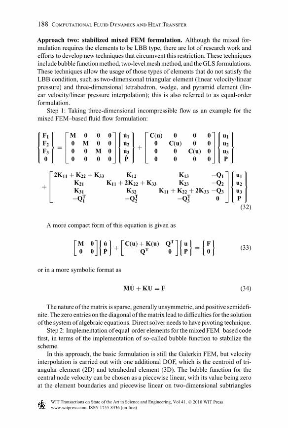
Approach two: stabilized mixed FEM formulation. Although the mixed for-mulation requires the elements to be LBB type, there are lot of research work andefforts to develop new techniques that circumvent this restriction. These techniquesinclude bubble function method, two-level mesh method, and the GLS formulations.These techniques allow the usage of those types of elements that do not satisfy theLBB condition, such as two-dimensional triangular element (linear velocity/linearpressure) and three-dimensional tetrahedron, wedge, and pyramid element (lin-ear velocity/linear pressure interpolation); this is also referred to as equal-orderformulation.
Step 1: Taking three-dimensional incompressible flow as an example for themixed FEM–based fluid flow formulation:⎧⎪⎪⎨⎪⎪⎩
F1F2F30
⎫⎪⎪⎬⎪⎪⎭ =
⎡⎢⎢⎣M 0 0 00 M 0 00 0 M 00 0 0 0
⎤⎥⎥⎦⎧⎪⎪⎨⎪⎪⎩
u1u2u3
P
⎫⎪⎪⎬⎪⎪⎭ +
⎡⎢⎢⎣C(u) 0 0 0
0 C(u) 0 00 0 C(u) 00 0 0 0
⎤⎥⎥⎦⎧⎪⎪⎨⎪⎪⎩
u1u2u3P
⎫⎪⎪⎬⎪⎪⎭
+
⎡⎢⎢⎣2K11 + K22 + K33 K12 K13 −Q1
K21 K11 + 2K22 + K33 K23 −Q2K31 K32 K11 + K22 + 2K33 −Q3
−QT1 −QT
2 −QT3 0
⎤⎥⎥⎦⎧⎪⎪⎨⎪⎪⎩
u1u2u3P
⎫⎪⎪⎬⎪⎪⎭(32)
A more compact form of this equation is given as
[M 00 0
]{uP
}+
[C(u) + K(u) QT
−QT 0
]{uP
}=
{F0
}(33)
or in a more symbolic format as
MU + KU = F (34)
The nature of the matrix is sparse, generally unsymmetric, and positive semidefi-nite. The zero entries on the diagonal of the matrix lead to difficulties for the solutionof the system of algebraic equations. Direct solver needs to have pivoting technique.
Step 2: Implementation of equal-order elements for the mixed FEM–based codefirst, in terms of the implementation of so-called bubble function to stabilize thescheme.
In this approach, the basic formulation is still the Galerkin FEM, but velocityinterpolation is carried out with one additional DOF, which is the centroid of tri-angular element (2D) and tetrahedral element (3D). The bubble function for thecentral node velocity can be chosen as a piecewise linear, with its value being zeroat the element boundaries and piecewise linear on two-dimensional subtriangles
www.witpress.com, ISSN 1755-8336 (on-line) WIT Transactions on State of the Art in Science and Engineering, Vol 41, © 20 WIT Press10

Sunden CH005.tex 10/9/2010 15: 0 Page 189
Equal-order segregated finite-element method 189
Figure 5.3. Bubble function for linear triangular and tetrahedral elements.
or three-dimensional subtetrahedron. The pressure is interpolated linearly over theelement (Figure 5.3).
Step 3: Implementation of stabilized FEM formulation GLS for two-dimensional and three-dimensional fluid flow using two-dimensional and three-dimensional degenerated elements, i.e., using equal-order interpolation (linearvelocity/linear pressure) for both velocity and pressure.
The GLS variation form of the momentum and continuity equation is given by∫�
w · (ρ0u · ∇u)dx +∫�
∇w · (−P + 2µD(u))dx −∫�
ρ0wfdx + Q∇ · udx
+nel∑
n=1
∫�n
RGLSdx = −∫�
wTids (35)
Here, w and Q are the weight functions for the momentum equation and thecontinuity equation, respectively. The element residual is defined as
RGLS = (τSUPGρ0u · ∇w + τPSPG∇Q − τGLS2µD(w))
· (ρ0u · ∇u + ∇P − 2µD(u)) (36)
The τ coefficients are weighting parameters, which could be functions of theelement size, element Reynolds number, and/or element average velocity. If thesecoefficients are selected properly, equal-order elements can be used and LBBcondition is not necessary.
For momentum equation, the final equations are given by
(C(u) + CSUPG(u) + CGLS(u))u + (K + KSUPG + KGLS)u
− (Q + QSUPG + QGLS)P = F (37)
For continuity equation, we have
−QTu − QPSPGP + CPSPG(u)u + KPSPGu = 0 (38)
www.witpress.com, ISSN 1755-8336 (on-line) WIT Transactions on State of the Art in Science and Engineering, Vol 41, © 20 WIT Press10

Sunden CH005.tex 10/9/2010 15: 0 Page 190
190 Computational Fluid Dynamics and Heat Transfer
Galerkin/least-squares formulationThe stability of the mixed Galerkin finite element for incompressible flows can beenhanced by the addition of various least-squares terms to the original Galerkinvariational statement. The Galerkin/Least-squares approach is sometimes termeda residual method because the added least-squares terms are weighted residualsof the momentum equation; this form of the least-squares term implies the con-sistency of the method since the momentum residual is employed. The GLS – aPetrov–Galerkin method – is also known as a perturbation method since the addedterms can be viewed as perturbations to the weighting functions. Development andpopularization of the GLS methods for flow problems are primarily due to Hughes,Tezduyar, and co-workers and are a generalization of their work on SUPG andPSPG methods.
The usual approach to the GLS begins with the discontinuous approximation intime Galerkin method and considers a finite-element approximation for a space–time slab. Continuous polynomial interpolation is used for the spatial variationwhile a discontinuous time function is used within the space–time slab. The assumedtime representation obviates the need to independently consider time integrationmethods. To simplify the present discussion of the GLS, the time independent formof the incompressible flow problem is considered which avoids the complexity ofthe space–time finite-element formulation. Using vector notation and followingthe weak form development, the GLS variational form for the momentum andcontinuity equations can be written as∫�
Nm(ρu · ∇u)dx +∫�
∇Nm · ( − P + 2µ∇D(u)dx −∫�
ρNmfxdx +∫�
Nn∇ · u)dx
+nel∑
n=1
∫�
RGLS = −∫�
Nmτidsdx (39)
where Nm and Nn are the weight functions for the momentum and continuityequations and the element residual is defined by
RGLS = (δ+ ε+ β) · (ρu · ∇u + ∇(P − 2µ∇D(u)) (40)
δ= τSUPGu · ∇Nm
ε= τPSPG1
ρ∇Nn
β= − τGLS2µ∇(D(Nm))The τ coefficients are weighting parameters; if the definitions for δ, ε, and β
are substituted into equation (40) and the various weighting parameters are madeequivalent to a single parameter τ, the RGLS will be
RGLS = τ[ρu · ∇Nm + ∇Nn − 2µ∇ · D(u)] · [ρu · ∇u + ∇(P − 2µ∇ · D(u)] (41)
www.witpress.com, ISSN 1755-8336 (on-line) WIT Transactions on State of the Art in Science and Engineering, Vol 41, © 20 WIT Press10

Sunden CH005.tex 10/9/2010 15: 0 Page 191
Equal-order segregated finite-element method 191
This is the standard definition for the residual contribution to the GLS formula-tion. The splitting of the first residual into three separate contributions in equation(41) was done to allow the original SUPG and PSPG formulations to be easilyrecovered.
If β and ε are set to zero, the stabilized SUPG method is recovered.If β and δ are set to zero, the stabilized PSPG method is recovered.If only β is set to zero, both SUPG and PSPG stabilization methods are
recovered.Note that in equation (39) the first four integrals and the right-hand side define a
standard Galerkin-weighted residual method that is written in terms of global shapefunctions; the integrals are over the simulation domain which is composed by thediscretized finite elements. The added residual term in equation (39) is defined overthe interior of each element and basically contains the square of all or parts of themomentum residual. The various τ parameters are positive coefficients that havethe dimension of time. The forms of these parameters are usually developed fromerror estimates, convergence proofs, and dimensional analysis. Particular constantswithin each parameter are selected by optimizing the method on simple problemsand generalizing to multidimensions. It should be noted that the development ofthe τ parameters is not a unique process. For the steady problems considered herea typical τ for the GLS method is
τ =[(
2‖u‖h
)2
+(
4ν
h2
)2]−1/2
(42)
where h is an appropriate element length. For the SUPG and PSPG formulations,the τ values are the function of an element Reynolds number and the ratio of anelement length to a velocity scale.
The error and convergence analyses for the GLS and PSPG methods havedemonstrated that the equal-order velocity and pressure interpolation for thesemethods is viable and the LBB condition is not required [6]. In finite-elementimplementation, convenient elements, such as the bilinear Q1/Q1, linear P1/P1,biquadratic Q2/Q2, and quadratic P2/P2, are now useful approximations whilebeing unstable in the Galerkin finite-element context. The low-order elements havean advantage over their higher-order counterparts because some of the stabiliza-tion terms associated with viscous diffusion are identically zero. This considerablysimplifies the element equation building process.
The matrix form of velocity–pressure equationsThe matrix form of the stabilized GLS formulation could be summarized as theMomentum equation and Continuity equation, respectively.Momentum: (C(u) + Cδ(u) + Cβ(u)}u + (K + Kδ+ Kβ)u − (Q + Qδ+ Qβ)P = FContinuity: − QT u − QεP + (Cε(u) + Kε)u = 0
Expended discretization form of equations for velocity–pressure coupling andSUPG stabilization, which are summarized in Table 5.3, will be used as the base
www.witpress.com, ISSN 1755-8336 (on-line) WIT Transactions on State of the Art in Science and Engineering, Vol 41, © 20 WIT Press10

Sunden CH005.tex 10/9/2010 15: 0 Page 192
192 Computational Fluid Dynamics and Heat Transfer
Table 5.3. Element-level matrices
M =∫�e
ρNmNnd�e C(u) =∫�e
ρNmuj∂Nn
∂xjd�e
Su(u) =∫�e
[ρτsui
∂Nm
∂xi
]uj∂Nn
∂xjd�e Spi(u) =
∫�e
[τsuj
∂Nm
∂xj
]∂Nn
∂xid�e
Kij =∫�e
µ∂Nm
∂xj
∂Nn
∂xid�e Qi =
∫�e
∂Nm
∂xiNnd�e
Sδij =∫�e
ρδ∂Nm
∂xi
∂Nn
∂xjd�e Kτi (u) =
∫�e
τp∂Nm
∂xi
[uj∂Nn
∂xj
]d�e
Qτ =∫�e
τp
ρ
[∂Nm
∂xj
∂Nn
∂xj
]d�e SFi(u) =
∫�e
ρτs
[uj∂Nm
∂xj
]d�e fbi
SF4 =∫�e
τp
[fbj∂Nm
∂xj
]d�e Fi =
∫∂�e
Nm�id�e +∫∂�e
ρNm fBid�e
for our further segregated formulation in the next chapter.
⎡⎢⎢⎣M1
M2M3
0
⎤⎥⎥⎦⎧⎪⎪⎪⎪⎨⎪⎪⎪⎪⎩
˙u˙v˙w˙p
⎫⎪⎪⎪⎪⎬⎪⎪⎪⎪⎭
+
⎡⎢⎢⎢⎣C(u) + Su(u) Sp1(u)
C(u) + Su(u) Sp2(u)C(u) + Su(u) Sp3(u)
−Kτ1 (u) −Kτ2 (u) −Kτ3 (u) 0
⎤⎥⎥⎥⎦⎧⎪⎪⎪⎨⎪⎪⎪⎩
uvwp
⎫⎪⎪⎪⎬⎪⎪⎪⎭
+
⎡⎢⎢⎢⎣2K11 + K22 + K33 K12 K13 −Q1
K21 K11 + 2K22 + K33 K23 −Q2
K31 K32 K11 + K22 + 2K33 −Q3
−QT1 −QT
2 −QT3 0
⎤⎥⎥⎥⎦⎧⎪⎪⎪⎨⎪⎪⎪⎩
uvwp
⎫⎪⎪⎪⎬⎪⎪⎪⎭
+
⎡⎢⎢⎢⎣Sδ11 Sδ12 Sδ13 0Sδ21 Sδ22 Sδ23 0Sδ31 Sδ32 Sδ33 0
0 0 0 −Qτ
⎤⎥⎥⎥⎦⎧⎪⎪⎪⎨⎪⎪⎪⎩
uvwp
⎫⎪⎪⎪⎬⎪⎪⎪⎭ =
⎧⎪⎪⎪⎨⎪⎪⎪⎩F1
F2
F3
0
⎫⎪⎪⎪⎬⎪⎪⎪⎭ +
⎧⎪⎪⎪⎨⎪⎪⎪⎩SF1 (u)SF2 (u)SF3 (u)−SF4
⎫⎪⎪⎪⎬⎪⎪⎪⎭ (43)
It is noted that since all of the SUPG τ parameters depend on the elementsize, in the limit as the element size gets smaller, the stabilized method reduces to
www.witpress.com, ISSN 1755-8336 (on-line) WIT Transactions on State of the Art in Science and Engineering, Vol 41, © 20 WIT Press10

Sunden CH005.tex 10/9/2010 15: 0 Page 193
Equal-order segregated finite-element method 193
the Galerkin form. In another words, stabilization plays a significant role only forcoarse mesh.
5.4 Formulation of Stabilized Equal-OrderSegregated Scheme
This section discusses the strategies for the solution of large systems of equationsarising from the finite-element discretization of the formulations. To solve thenonlinear fluid flow and heat transfer problem, particular emphasis is placed onsegregated scheme in nonlinear level and iterative methods in linear level. Thereality of velocity–pressure coupling formulation in the last section not only resultsin a large dimensioned system but also generates a stiffness matrix radically differentto the narrowband type of matrix, which is inefficient to solve and the advectionterm causes solution instability.
The first part in the section is the kernel part; it is a uniformed consistent solutionscheme for nonlinear and linear level to support any fluid flow/heat transfer andtransport phenomena. The combination of “segregated scheme,” “iterative solver,”and “Block I/O” composes the whole solution picture in a very efficient and robustway. First, the decoupled pressure–velocity segregated scheme is discussed andexpended in very detail under finite-element method by nonlinear level, and thenthe Generalized Minimum Residual Method (GMRES)-based iterative techniqueand matrix preconditioners are used to solve linear equations. With respect to imple-mentation, the condensed storage and block I/O technique is demonstrated to boostsolution efficiency especially for large systems.
5.4.1 Introduction
Several categorizations can be made by using finite-element method to solve theNavier–Stokes equation for fluid flow and thermal problems. They are mainly(a) velocity–pressure coupling and (b) orders of interpolation functions forvelocity and pressure.
The first categorization is based on how the primitive variables of velocityand pressure are treated. The solution schemes are categorized into three groups:velocity–pressure integrated method, penalty method, and segregated velocity–pressure method. The velocity–pressure integrated scheme treats velocity andpressure simultaneously; it needs less iteration number in nonlinear level, but largerglobal matrix requires longer execution time and a large memory in linear level; andusually its overall runtime performance is slow. The penalty scheme eliminates thedirect pressure computation by introducing penalty function, thus speeding up theexecution time and memory requirement; however, pressure field from simple post-process is not satisfying especially for large Reynolds number fluid flow problem.Recently, much attention has been paid to the segregated velocity–pressure scheme,where velocity and corresponding pressure field are computed alternatively in aniterative sequence. This scheme has the advantage of speed and memory usage with
www.witpress.com, ISSN 1755-8336 (on-line) WIT Transactions on State of the Art in Science and Engineering, Vol 41, © 20 WIT Press10

Sunden CH005.tex 10/9/2010 15: 0 Page 194
194 Computational Fluid Dynamics and Heat Transfer
the price of complicated formulation and possible less solution robustness due tovelocity–pressure decoupling (addressed later).
The second categorization is based on the mixed-order interpolation and equal-order interpolation according to the orders of interpolation functions for the velocityand pressure in element level. The mixed-order interpolation attempts to eliminatethe tendency to produce checkerboard pressure pattern and to satisfy LBB condi-tion; the velocity in this method is interpolated linearly, whereas the pressure isassumed to be constant; this interpolation is referred to as Q1P0. The equal-orderinterpolation in Ref. [5] uses linear interpolation for velocity–pressure formulation(referred to as Q1P1) without exhibiting spurious pressure modes, by employingnonconsistent pressure equations (NCPEs) for pressure correction. This methodmakes the solver more effective than constant element pressure in an element forQ1P0 method.
The objective of this chapter is to explore further the merits of the finite-elementmethods in simulating the flow where the upstream effects play important roles.Thus, we are presenting the details of making use of both the segregated velocity–pressure and equal-order formulations on the basis of SUPG method.
The basic idea of segregated algorithms is to decouple the pressure calculationfrom the velocity calculation by taking the divergence of the vector momentumequation and applying some clever insights regarding incompressible flow. Earlymotivation for this approach was largely twofold: to mitigate memory requirementsof fully coupled algorithms and to enable semi-implicit time integration.
Pressure–velocity segregation methods have been reviewed by severalresearchers in the context of the finite-element method; most notable are the papersby Gresho and Haroutunian et al. [2]. Basically, all current segregated algorithmvariants are distinguished by the way in which the pressure is decoupled and pro-jected from one time step to the next. Haroutunian and Engelman [2] proposed threeconsistent finite-element counterparts to the SIMPLE and SIMPLER algorithm.To further reduce the size of the submatrix systems, each individual componentof the momentum equations was solved separately and successively by iterativetechniques. Overall at each Newton iteration or Picard iteration they solved fourmatrix subsystems, one for each of three velocity components and one for thepressure. Interestingly, the most challenging matrix system to solve happens to beone arising from the discretization of the pressure equation; here, the right-handside SF4 in equation (5.43) is lagged from the last iteration so that this equationis solved solely for the pressure. The resulting matrix, despite being symmet-ric, is actually very poorly conditioned due to poor scaling. Nonetheless, thesechallenging matrix systems can be readily solved by modern iterative solvers andreordering/preconditioner strategies, and the success of this algorithm over the lastdecade has been enormous.
In our view this approach is still a compromise to the favorable convergenceproperties of a fully coupled technique advocated here. Convergence to stable solu-tions at successive time steps is linear at best case and sometimes asymptotic,sometimes resulting in large number of required segregation iterations (albeit fastiterations). Moreover, the method introduces several relaxation parameters that
www.witpress.com, ISSN 1755-8336 (on-line) WIT Transactions on State of the Art in Science and Engineering, Vol 41, © 20 WIT Press10

Sunden CH005.tex 10/9/2010 15: 0 Page 195
Equal-order segregated finite-element method 195
must be tuned to the application. If one chooses alternatives to the primitive vari-able formulation, then boundary conditions on velocity become challengeable toapply accurately. Finally, codes centered around this algorithm are more complex instructure, as they still contain the intricacies of matrix solution services but involvemore than one data structure (for the mixed interpolation) and more inner and outeriteration loops.
5.4.2 FEM-based segregated formulation
This formulation is based on the algorithm of Rice and Schnipke’s [5] and Shaw’s [7]pioneer works; they use non-consistent pressure equations (NCPE) for the pressurestep and pressure correction step rather than the conventional weak form of the flowequations resulting from Galerkin finite element context. This approach has gainedpopularity in recent years with the very desirable advantage of precluding spuriouspressure modes from pressure solution. This consequently allows them to employthe desirable feature of “equal-order interpolation for the velocity and pressure.”For this reason, the algorithm can solve the flow without using very refined meshesand hybrid element types highly desirable for commercial code obtained from CADmodel. However, the expanse of this algorithm includes the extra work of imposingboundary conditions properly and their complex formulation. In this section, weshow the formulation derivation details starting from the N–S equation.
Bilinear interpolationThe fluid flow continuity equation and the momentum equation follow same formas listed in Section 3.1. For implementation using finite-element method, velocityand pressure at arbitrary position could be interpolated using “equal-order bilinearinterpolation” to adapt brick or other degenerated elements.
u(x, y) = Niui (44a)
v(x, y) = Nivi (44b)
w(x, y) = Niwi (44c)
p(x, y) = Nipi (44d)
Discretization and system assemblyUsing the standard Galerkin approach, the momentum equation is multiplied byweighting functions, and using the Green–Gauss theorem, the diffusion terms areintegrated by parts in x momentum equation as follows:∫
�
ρN
(u∂u
∂x+ v∂u
∂y+ w
∂u
∂z
)d� = −
∫�
N∂p
∂xd�+
∫�
NFxd�
(45)
+ µ∫�
N
[∂2u
∂x2 + ∂2u
∂y2 + ∂2u
∂z2
]d�
www.witpress.com, ISSN 1755-8336 (on-line) WIT Transactions on State of the Art in Science and Engineering, Vol 41, © 20 WIT Press10

Sunden CH005.tex 10/9/2010 15: 0 Page 196
196 Computational Fluid Dynamics and Heat Transfer
Construct a function,
∫�
⎡⎢⎢⎣∂(∂u
∂xN
)∂x
+∂
(∂u
∂yN
)∂y
+∂
(∂u
∂zN
)∂z
⎤⎥⎥⎦d�(46)
=∫�
(∂u
∂x
∂N
∂x+ ∂u
∂y
∂N
∂y+ ∂u
∂z
∂N
∂z
)d�+
∫�
N
(∂2u
∂x2 + ∂2u
∂y2 + ∂2u
∂z2
)d�
Using Green–Gauss theorem,
∫�
⎡⎢⎢⎣∂(∂u
∂xN
)∂x
+∂
(∂u
∂yN
)∂y
+∂
(∂u
∂zN
)∂z
⎤⎥⎥⎦d� =∫�
N
(∂u
∂xnx + ∂u
∂yny + ∂u
∂znz
)d�
(47)
Equations (45), (46), and (47) are combined to get the new form of thediscretized x-momentum equation:∫�
ρN
(u∂u
∂x+ v∂u
∂y+ w
∂u
∂z
)d� = −
∫�
N∂p
∂xd�+
∫�
NFxd�
+∫�
N
(∂u
∂xnx + ∂u
∂yny + ∂u
∂znz
)d�−
∫�
(∂u
∂x
∂N
∂x+ ∂u
∂y
∂N
∂y+ ∂u
∂z
∂N
∂z
)d�
Move the last item in the right-hand side to the left-hand side, then
LHS = [Au]{u} =∫�
[ρN
(u∂u
∂x+ v∂u
∂y+ w
∂u
∂z
)+
(µ∂u
∂x
∂N
∂x+ µ∂u
∂y
∂N
∂y+ µ∂u
∂z
∂N
∂z
)]d�
= ρ∫�
Ni
[u∂Nj
∂x+ v∂Nj
∂y+ w
∂Nj
∂z
]d�{u} +
[∫�
µ∂Ni
∂x
∂Nj
∂xd�
]{u}
+[∫�
µ∂Ni
∂y
∂Nj
∂yd�
]{u} +
[∫�
µ∂Ni
∂z
∂Nj
∂zd�
]{u}
= [C(u, v, w) + K11 + K22 + K33]{u} (48a)
where, C(U ) is the advection item and K11, K22, K33 are the diffusion items.To obtain C(U ), velocities u, v, w are considered the average values in an element.
RHS = −∫�
Ni∂p
∂xd�+
∫�
NiFxd�+∫�
Ni
(∂u
∂xnx + ∂u
∂yny + ∂u
∂znz
)d� = −M14{p} + {F�xA} + {Fx} (48b)
[Av] and [Aw] could be achieved by similar approaches.
www.witpress.com, ISSN 1755-8336 (on-line) WIT Transactions on State of the Art in Science and Engineering, Vol 41, © 20 WIT Press10

Sunden CH005.tex 10/9/2010 15: 0 Page 197
Equal-order segregated finite-element method 197
SUPG items The SUPG weighting function proposed by Brooks is defined by:Wk = Nk + pk
Here the streamline-upwind contribution pk is defined as:
pk = ke
(ue1)2 + (ue
2)2
(ue
j∂Ni
∂xj
)(49)
Only convective items are weighted with the SUPG functions for the inconsistentapproach, which is believed to be more stable than the consistent SUPG formulation[10]. The extra items from pk should be added into K11, K22, K33 in equation (49)in the implementation.
Equation of pseudo velocity (prediction phase)In matrix form of the segregated momentum equations:
[M11]{u} = −[M14]{p} + {F�xA} + {Fx} (50a)
[M22]{v} = −[M24]{p} + {F�yA} + {Fy} (50b)
[M33]{w} = −[M34]{p} + {F�zA} + {Fz} (50c)
where
[M11] = [C(u, v, w) + K11 + K22 + K33] + [SUPG(u, v, w)]
[M22] = [C(u, v, w) + K11 + K22 + K33] + [SUPG(u, v, w)]
[M33] = [C(u, v, w) + K11 + K22 + K33] + [SUPG(u, v, w)]
[M14] =∫�
Ni∂p
∂xd�
[M24] =∫�
Ni∂p
∂yd�
[M34] =∫�
Ni∂p
∂zd�
{F�xA} =∫�
Ni
(∂u
∂xnx + ∂u
∂yny + ∂u
∂znz
)d�
{F�yA} =∫�
Ni
(∂u
∂xnx + ∂u
∂yny + ∂u
∂znz
)d�
{F�zA} =∫�
Ni
(∂u
∂xnx + ∂u
∂yny + ∂u
∂znz
)d�
{Fx} =∫�
NiFxd�
{Fy} =∫�
NiFyd�
{Fz} =∫�
NiFzd�
where � is the fluid domain (volume); and � is the flow boundaries (surface).There are no SUPG items in {Fx}{Fy}{Fz} for the inconsistent approach.
www.witpress.com, ISSN 1755-8336 (on-line) WIT Transactions on State of the Art in Science and Engineering, Vol 41, © 20 WIT Press10
Sunden CH005.tex 10/9/2010 15: 0 Page 198
198 Computational Fluid Dynamics and Heat Transfer
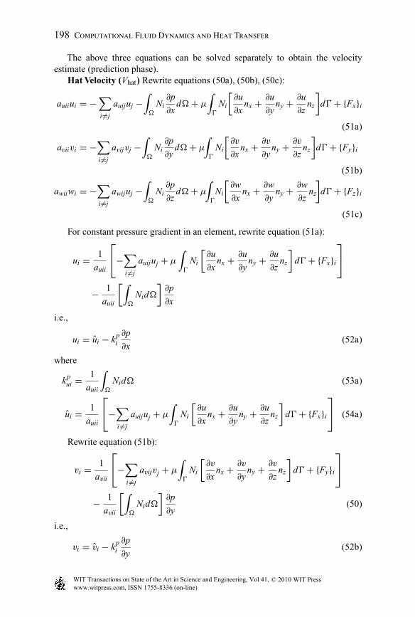
The above three equations can be solved separately to obtain the velocityestimate (prediction phase).
Hat Velocity (Vhat) Rewrite equations (50a), (50b), (50c):
auiiui = −∑i �=j
auijuj −∫�
Ni∂p
∂xd�+ µ
∫�
Ni
[∂u
∂xnx + ∂u
∂yny + ∂u
∂znz
]d�+ {Fx}i
(51a)
aviivi = −∑i �=j
avijvj −∫�
Ni∂p
∂yd�+ µ
∫�
Ni
[∂v
∂xnx + ∂v
∂yny + ∂v
∂znz
]d�+ {Fy}i
(51b)
awiiwi = −∑i �=j
awijuj −∫�
Ni∂p
∂zd�+ µ
∫�
Ni
[∂w
∂xnx + ∂w
∂yny + ∂w
∂znz
]d�+ {Fz}i
(51c)
For constant pressure gradient in an element, rewrite equation (51a):
ui = 1
auii
⎡⎣−∑i �=j
auijuj + µ∫�
Ni
[∂u
∂xnx + ∂u
∂yny + ∂u
∂znz
]d�+ {Fx}i
⎤⎦− 1
auii
[∫�
Nid�
]∂p
∂x
i.e.,
ui = ui − kpi∂p
∂x(52a)
where
kpui = 1
auii
∫�
Nid� (53a)
ui = 1
auii
⎡⎣−∑i �=j
auijuj + µ∫�
Ni
[∂u
∂xnx + ∂u
∂yny + ∂u
∂znz
]d�+ {Fx}i
⎤⎦ (54a)
Rewrite equation (51b):
vi = 1
avii
⎡⎣−∑i �=j
avijvj + µ∫�
Ni
[∂v
∂xnx + ∂v
∂yny + ∂v
∂znz
]d�+ {Fy}i
⎤⎦− 1
avii
[∫�
Nid�
]∂p
∂y(50)
i.e.,
vi = vi − kpi∂p
∂y(52b)
www.witpress.com, ISSN 1755-8336 (on-line) WIT Transactions on State of the Art in Science and Engineering, Vol 41, © 20 WIT Press10

Sunden CH005.tex 10/9/2010 15: 0 Page 199
Equal-order segregated finite-element method 199
where
kpvi = 1
avii
∫�
Nid� (53b)
vi = 1
avii
⎡⎣−∑i �=j
avijvj + µ∫�
Ni
[∂v
∂xnx + ∂v
∂yny + ∂v
∂znz
]d�+ {Fy}i
⎤⎦ (54b)
Rewrite equation (51c):
wi = 1
awii
⎡⎣−∑i �=j
awijwj + µ∫�
Ni
[∂w
∂xnx + ∂w
∂yny + ∂w
∂znz
]d�+ {Fz}i
⎤⎦− 1
awii
[∫�
Nid�
]∂p
∂z
i.e.,
w = wi − kpi∂p
∂z(52c)
where
kpwi = 1
awii
∫�
Nid� (53c)
wi = 1
awii
⎡⎣−∑i �=j
awijwj + µ∫�
Ni
[∂w
∂xnx + ∂w
∂yny + ∂w
∂znz
]d�+ {Fz}i
⎤⎦(54c)
To ensure mass continuity, the velocity should be updated (corrected) at eachiteration by which velocity correction is reformulated from the new pressure value,refer to equation 62a, 62b and 62c for velocity correction details.
VCorrected = Vhat + VCorrection_Term_By_Pressure (55)
Pressure Poisson equationOn applying Green–Gauss theorem and integration to the continuity equation,the integral of the divergence in a domain equals the net flux across the domainboundary: ∫
�
[∂(uN )
∂x+ ∂(vN )
∂y+ ∂(wN )
∂z
]d� =
∫�
N �v · �nd� (56)
The continuity equation becomes:∫�
N
(∂u
∂x+ ∂v
∂y+ ∂w
∂z
)d� = −
∫�
(∂N
∂xu + ∂N
∂yv+ ∂N
∂zw
)d�
(57)+
∫�
N (unx + vny + wnz)d� = 0
www.witpress.com, ISSN 1755-8336 (on-line) WIT Transactions on State of the Art in Science and Engineering, Vol 41, © 20 WIT Press10

Sunden CH005.tex 10/9/2010 15: 0 Page 200
200 Computational Fluid Dynamics and Heat Transfer
The modified continuity equation (57) using green function transformation istargeted to solve pressure.
Step 1: Substitute interpolated velocity from equations (44a), (44b), and (44c)to continuity equation (57)
−∫�
(∂Ni
∂x(Njuj) + ∂Ni
∂y(Njvj) + ∂Ni
∂z(Njwj)
)d�+
∫�
Ni(unx + vny + wnz)d� = 0
(58)
Step 2: Substitute velocity prediction from equations (53a), (53b), and (53c)into equation (58)∫�
[∂Ni
∂x
(NjK
pj∂p
∂x
)+ ∂Ni
∂y
(NjK
pj∂p
∂y
)+ ∂Ni
∂z
(NjK
pj∂p
∂z
)]d�
=∫�
(∂Ni
∂x(Njuj) + ∂Ni
∂y(Nj vj) + ∂Ni
∂z(Njwj)
)d�−
∫�
Ni(unx + vny + wnz)d�
(59)
Step 3: Rewrite to final formNotice that p = Nipi, so substituting ∂p
∂x = ∂(Nipi)∂x = pi
∂Ni∂x (assume that p is con-
stant in an element here) in equation (59) (using similar way for and ) we obtain∂p∂y and ∂p
∂z .{∫�
[∂Ni
∂x(Nk Kp
k )(∂Nj
∂x
)]d�+
∫�
[∂Ni
∂y(Nk Kp
k )∂Nj
∂y
]d�
+∫�
[∂Ni
∂z(Nk Kp
k )∂Nj
∂z
]d�
}· {p}
(60)
=∫�
∂Ni
∂x(Njuj)d�+
∫�
∂Ni
∂y(Nj vj)d�+
∫�
∂Ni
∂z(Njwj)d�
−∫�
Ni(unx + vny + wnz)d�
Moving Vhat out of the integration in equation (60), we obtain:{∫�
[∂Ni
∂x(Nk Kp
k )(∂Nj
∂x
)]d�+
∫�
[∂Ni
∂y(Nk Kp
k )∂Nj
∂y
]d�
+∫�
[∂Ni
∂z(Nk Kp
k )∂Nj
∂z)]
d�
}· {p}
(61)
=∫�
∂Ni
∂xNjd�{u} +
∫�
∂Ni
∂yNjd�{v} +
∫�
∂Ni
∂zNjd�{w}
−∫�
Ni(unx + vny + wnz)d�
Now equation (61) is the final form of pressure Poisson equation.
www.witpress.com, ISSN 1755-8336 (on-line) WIT Transactions on State of the Art in Science and Engineering, Vol 41, © 20 WIT Press10

Sunden CH005.tex 10/9/2010 15: 0 Page 201
Equal-order segregated finite-element method 201
It is interesting to note that the element pressure matrices are identical tothose obtained in classical diffusion-type problems, with the term K replacingthe diffusion coefficient.
Here are more discussions on segregated solution scheme.
(1) The coefficient matrix for the pressure equation is similar to that obtained forthe diffusion term in the conventional finite-element formulation if the viscosityis replaced by NiK
pj the formulation developed by Rice [5] and Vellando [12];
this fact is indicative of the stability and robust nature of the resulting pressurefield.
(2) The LHS and RHS of equation (69) could be constructed and evaluated inelement level and then assembled into global matrix LHS and RHS; this istypical finite-element behavior.
(3) In equation (60), kpi is a node-based property, it should be assembled from
the saved element-level matrix,∫�
Nid�, auii is also a global property fromassembly.
(4) Equation (60) is in the form of Poisson equation; the LHS matrix has theproperties of symmetric and positive definite as indicated by Shaw [7].
(5) Special boundary integrations on all inflow and outflow boundaries are requiredto solve pressure, which corresponds to the fourth item in equation (61).
Velocity correctionWrite equations (51a), (51b), and (51c) using weighting function p(x,y) = Nipi andchain law, and discarding velocity gradient items on boundaries. ui, vi, wi are usedfor the velocity prediction as “hat” velocity.
ui = 1
auii
⎡⎣−∑i �=j
auijuj + {Fx}i
⎤⎦ − 1
auii
[∫�
Ni∂Nj
∂xd�
]{p}
Or, ui = ui − 1
auii
[∫�
Ni∂Nj
∂xd�
]{p} = ui − 1
auii{M14}{p} (62a)
Get corrected velocity v, w in the same way as u,
vi = vi − 1
avii
[∫�
Ni∂Nj
∂yd�
]{p} = vi − 1
avii{M24}{p} (62b)
wi = wi − 1
awii
[∫�
Ni∂Nj
∂zd�
]{p} = wi − 1
awii{M34}{p} (62c)
At this step, u, v, w are directly corrected from the predicted and with trivialeffort, the second item is the pressure coupling effect on the velocity.
Special treatments on boundary conditionsThere are some special treatments in the segregated formulation.
Wall boundary: For wall boundary, the surface integral or natural boundarycondition for the pressure equation is zero. To incorporate the known velocities into
www.witpress.com, ISSN 1755-8336 (on-line) WIT Transactions on State of the Art in Science and Engineering, Vol 41, © 20 WIT Press10

Sunden CH005.tex 10/9/2010 15: 0 Page 202
202 Computational Fluid Dynamics and Heat Transfer
pressure equation, it is required that “hat” velocity be zero. In implementation, thepressure coefficients, kp
ui, kpvi, kp
wi at the wall nodes should be set as zero.Specified velocity boundary: The surface integration of velocity boundary
conditions should be added into the pressure equation (61)’s right hand side as in thefourth item in the right hand side; for specified velocity boundary, the contributionis fixed.
Inflow/Outflow boundary Zero gradient velocity boundary condition is appliedat the inflow/outflow boundaries (including inlet/outlet boundary and pressureboundary), i.e., no special treatment in the momentum equation is required atthis kind of boundary. However, the contribution from the surface integration ofnatural boundary conditions should be added to the right-hand side of the pressureequation as done in the fourth item on the right-hand side of equation (60).
Segregated scheme not only simply divides the big coupling matrix into smallermatrices, but also sets up a pressure equation (Poisson equation) with positive-definite symmetric properties, which can greatly expedite the pressure solutionwith better accuracy. Most of the fluid flow problems are driven by pressure, andtherefore the velocity components will follow a good solution of pressure in practice.
Solution stability controlInertial relaxation. Inertial relaxation is used in the governing equations to slowdown the convergence rate in the same manner as transit terms are used in nonsteadyproblems, so the inertial relaxation factor is also called virtual time step.
The inertial relaxation is added to the governing equations in the followingmanner: [
Aii + ρi∫
Nd�
�tinertia
]φi +
∑j �=i
Aijφj = Fi + ρi∫
Nd�
�tinertiaφiold (63)
The second term in parentheses and the last term on the right-hand side are theinertial relaxation terms. �tinertia can be automatically adjusted according to theglobal matrix condition number.
• Small �tinertia value will enhance the solution stability and slow down theconvergence rate.
• �tinertia is applied to momentum equations only, and it will indirectly affect thepressure equation because of the slow marching of the velocity change.
• For convergence solution, the inertial term has no affect on the final solutionbecause it was eliminated in both LHS and RHS.
Explicit relaxation for momentum and pressure equations. Explicit relaxationfor momentum and pressure equations is the regular technique, which is also calledunder-relaxation. In this form, the new solution is weighted by the old solutionusing the formula:
φ = (1 − α)φold + αφnew (64)
where φnew is the updated current solution and φold is the previous value. α is therelaxation factor. If α= 1, all previous values are ignored, and all updated values are
www.witpress.com, ISSN 1755-8336 (on-line) WIT Transactions on State of the Art in Science and Engineering, Vol 41, © 20 WIT Press10
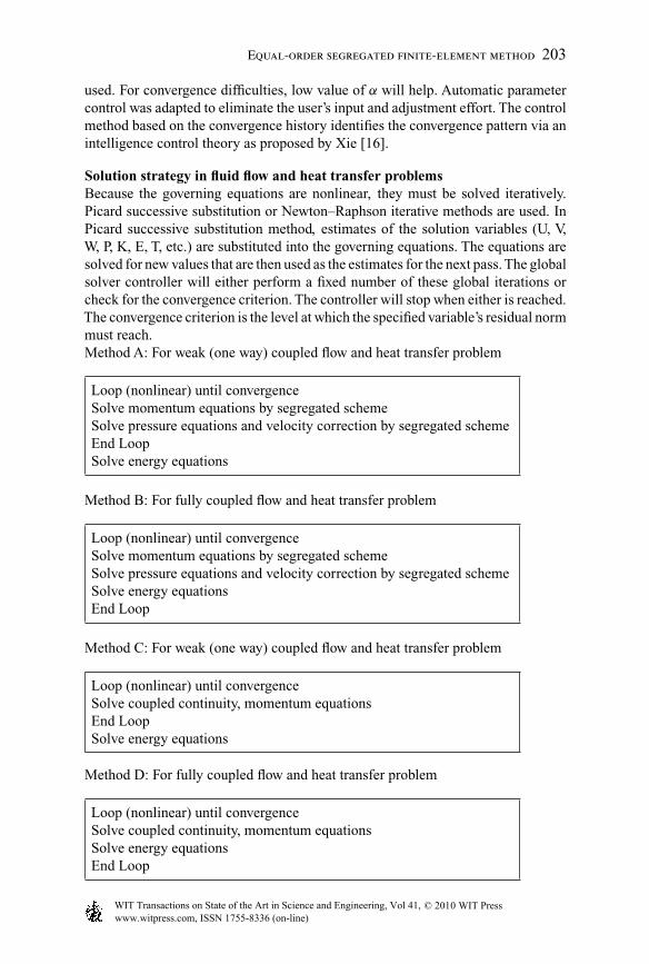
Sunden CH005.tex 10/9/2010 15: 0 Page 203
Equal-order segregated finite-element method 203
used. For convergence difficulties, low value of α will help. Automatic parametercontrol was adapted to eliminate the user’s input and adjustment effort. The controlmethod based on the convergence history identifies the convergence pattern via anintelligence control theory as proposed by Xie [16].
Solution strategy in fluid flow and heat transfer problemsBecause the governing equations are nonlinear, they must be solved iteratively.Picard successive substitution or Newton–Raphson iterative methods are used. InPicard successive substitution method, estimates of the solution variables (U, V,W, P, K, E, T, etc.) are substituted into the governing equations. The equations aresolved for new values that are then used as the estimates for the next pass. The globalsolver controller will either perform a fixed number of these global iterations orcheck for the convergence criterion. The controller will stop when either is reached.The convergence criterion is the level at which the specified variable’s residual normmust reach.Method A: For weak (one way) coupled flow and heat transfer problem
Loop (nonlinear) until convergenceSolve momentum equations by segregated schemeSolve pressure equations and velocity correction by segregated schemeEnd LoopSolve energy equations
Method B: For fully coupled flow and heat transfer problem
Loop (nonlinear) until convergenceSolve momentum equations by segregated schemeSolve pressure equations and velocity correction by segregated schemeSolve energy equationsEnd Loop
Method C: For weak (one way) coupled flow and heat transfer problem
Loop (nonlinear) until convergenceSolve coupled continuity, momentum equationsEnd LoopSolve energy equations
Method D: For fully coupled flow and heat transfer problem
Loop (nonlinear) until convergenceSolve coupled continuity, momentum equationsSolve energy equationsEnd Loop
www.witpress.com, ISSN 1755-8336 (on-line) WIT Transactions on State of the Art in Science and Engineering, Vol 41, © 20 WIT Press10

Sunden CH005.tex 10/9/2010 15: 0 Page 204
204 Computational Fluid Dynamics and Heat Transfer
Method E: For fully coupled flow and heat transfer problem
Loop (nonlinear) until convergenceSolve wholly coupled continuity, momentum and energy equationsEnd Loop
Owing to the importance of the segregated pressure–velocity solution schemeversus coupled scheme in most of the convective heat transfer problems, the majorityof computational efforts in heat transfer problems lie in solving the flow and pressurefields.
Scenario I demonstrates the decoupled flow and heat transfer, i.e., there areno temperature-dependent properties in the flow. We can first solve the isothermalflow (energy equation turned off) to yield a converged flow-field solution and thensolve the energy transport equation alone; this is a naturally segregated approach.Scenario II depicts the coupled flow and heat transfer (typically natural-convectionproblem); the common solution practice is to realize the flow–thermal couplingusing the nonlinear iteration until convergence. This is exactly the advantage of thevelocity–pressure “segregated scheme.”
Figure 5.4 shows the five solution schemes. Methods A and B are segregatedschemes described in this chapter, methods C and D are coupled momentumand pressure schemes, and method E is completely coupled velocity–pressure–temperature solution scheme. Method E is rarely used because of the bulk propertiesin global matrix by nature especially for large industry application. In any case, allmethods include solving energy equation.
For multiphysics system of equations to be solved by segregated manner, thesolution scheme is illustrated in Figure 5.4:
1. Velocity–pressure sequential solver (momentum-continuity)2. Turbulence subiteration3. Nonlinear iterations4. Time stepping iteration
At each time step, the nonlinear iterations are performed for the momentum-continuity, turbulence, front-tracking equation, and temperature. Subiterations ofturbulence transport equations are also used to accelerate the overall convergenceof the iterative process.
In more general and wider range multiphysics applications with structure, elec-tromagnetic, acoustics disciplines coupling with fluid flow and heat transfer, typicalapplication such as fluid–structure interaction (FSI), two-tier approaches may beapplied for the architecture with one unified simulation environment (workbench).In tier one, CFD package tightly integrate fluid flow, heat transfer, mass transfer, andacoustics components, and structure package tightly integrate linear dynamics andexplicit dynamics analysis components. In top level tier two, customized interpro-cess communication technology or general interprocess coupling tools like MPCCI
www.witpress.com, ISSN 1755-8336 (on-line) WIT Transactions on State of the Art in Science and Engineering, Vol 41, © 20 WIT Press10

Sunden CH005.tex 10/9/2010 15: 0 Page 205
Equal-order segregated finite-element method 205
(I)
(IV)
(II)
Solve u momentum
Solve v momentum
Solve w momentum
Solve pressure andcorrect velocity
Solve flow
Initial condition(IC)
Solve turbulence kineticenergy
Solve eddy dissipation
Update mt
Solve T (heat transfer)
Solve front tracking(free surface problem)
While t � tmax
(II)
(III)
Figure 5.4. General solution procedure of the segregated solver.
could be used for the communication among different independent packages suchas CFD, structure, electromagnetic analysis.
5.4.3 Data storage and block I/O process
Data storageThe FEM results in a system of linear equations containing a large number ofequations and unknown degree of freedom. A big amount of information requiresa clever data-keeping strategy to avoid whole matrix storage. Knowing that thesparse properties of global matrix, we are using data storing which is the so-calledskyline or column profile storage. Instead of storing every single matrix element,we could think of storing only the nonzero hits and corresponding position indexin the matrix assembly phase (Figure 5.5).
However, even with the use of such a reduced storage mode, the matrix is usuallyso large that it cannot be stored in core, so that it must be segmented in blocks andstored on low-speed disk storage.
www.witpress.com, ISSN 1755-8336 (on-line) WIT Transactions on State of the Art in Science and Engineering, Vol 41, © 20 WIT Press10

Sunden CH005.tex 10/9/2010 15: 0 Page 206
206 Computational Fluid Dynamics and Heat Transfer
X X
X X X
0
0 0
X X
X X X X
Figure 5.5. Skyline matrix structure.
Program Programbuffer
Operation systemarea
Systemcache
Outputfile
Figure 5.6. Block buffer I/O for disk writing.
Block I/O processImproving overall disk I/O performance can minimize both device I/O andactual CPU time. The techniques listed here can significantly improve FEA codeperformance.
The slowest process (routines) could be detected by using profiling tools such asAQTIME. After running a typical size of FEA model, the routines using most timein analysis, the top routines, and even lines are the processor bottleneck. These arethe targets to be improved for better performance.
“Block I/O” is a cost-efficient record buffer technique for large amount of datain the FEA processor. For writing, it saves a fixed number of element matrix infor-mation into buffer, and then writes the whole buffer into disk if the buffer is full,whereas reading is the reverse procedure. The buffer size is related to file system inoperation system and disk cache; we found that the optimal buffer size is 8 kbytesfor Windows XP WIN32 NTFS file system.
Here is an example for storage size calculation of one block element stiffnessmatrix with three-dimensional brick element (eight nodes) (Figure 5.6).Block size= 128 matrices* (8*8 entries/matrix) * 8 bits /entry= 65,536 bits= 65,536/8 bytes= 8,192 bytes
www.witpress.com, ISSN 1755-8336 (on-line) WIT Transactions on State of the Art in Science and Engineering, Vol 41, © 20 WIT Press10

Sunden CH005.tex 10/9/2010 15: 0 Page 207
Equal-order segregated finite-element method 207
Table 5.4. Data structure for Block I/O
Part ID Element type Data mapping Block numbers
Simulation Part 1 Tetrahedral Block 1 (32 kB) 6 blocks
domain elements Block 2
(4 nodes) Block 3
Block 4
Block 5
Block 6 Block 6
Other Block 1 (32 kB) 5 blocks
hybrid Block 2
elements Block 3
(8 nodes) Block 4
Block 5 Block 5
Part 2 Tetrahedral Block 1 (32 kB) 7 blocks
elements Block 2
(4 nodes) Block 3
Block 4
Block 5
Block 6 (32 kB)
Block 7 Block 7
Other hybrid Block 1 (32 kB) 3 blocks
elements Block 2 (32 kB)
(8 nodes) Block 3 Block 3
The data structure for block buffer I/O is shown in Table 5.4. The fluid domain iscomposed of multiple parts, while each part is decoded as the a group of tetrahedralelements and the a group of hybrid elements, hybrid element could be the com-bination of any brick, pyramid, wedge elements which could be considered as thedegraded element from eight-node brick element. For each group, 128*4 matricesfrom tetrahedral element composed a block; each matrix has 4*4 element entries,which also has the block size of 8 kbytes.
Because the fluid domain is composed of parts and each part has a differentnumber of brick element and tetrahedral element while the number may not be theeven times of the optimal block element number, a special counter was used if therewere a remainder of element number over block size number.
www.witpress.com, ISSN 1755-8336 (on-line) WIT Transactions on State of the Art in Science and Engineering, Vol 41, © 20 WIT Press10

Sunden CH005.tex 10/9/2010 15: 0 Page 208
208 Computational Fluid Dynamics and Heat Transfer
Apart from the efficient use of record buffers and disk I/O, some other tips asthe following were used in the code implementation:
(a) Using unformatted files instead of formatted files.(b) Writing whole arrays.(c) Using pointer shallow copy (pointer) instead of the complete deep copy.
By using the above-mentioned comprehensive methods, the I/O performancecan be dramatically improved, but when compared to other operations, it becomestrivial.
5.5 Case Studies
This section shows two examples of conjugate heat transfer problems where bothsolid and fluid are involved in the heat transfer analysis. The results are obtainedby using finite element–based equal-order segregated solution scheme discussed inthis chapter, and the SUPG stabilization term is enforced in both fluid and thermalprocessors.
For simple geometry, the high cell Peclet number did not cause severe problemfor the simulation results. That is because the temperature gradient in the flowdirection happened to be small for the natural boundary condition applied at theexit. Consequently, the numerical diffusion introduced by the discretization alsobecomes small. For complex geometry, however, heat transfer occurs through bothconvection and diffusion in all directions. Whenever the convection effects arestrong, the numerical oscillation of the computed temperature would happen if theGalerkin formulation were used.
The reason for this numerical difficulty has been well described. The conclu-sion basically is that the Galerkin formulation is of the same nature as the centralfinite difference scheme. It does not consider the influence of the flow velocity onthe temperature distribution in a cell through its basic interpolation functions. Toovercome this difficulty, either an upwind scheme or optimized upwind scheme(SUPG) should be adopted for the convection term. In the upwind schemes, a biasis given to the upwind nodal temperature by modifying the interpolation functionsaccording to the local fluid flow velocity, both the direction and the magnitude.
5.5.1 Two-dimensional air cooling box
The first example shown in Figure 5.7 is a two-dimensional square-shaped electronicbox with airflow cooling. Two small copper blocks are heat sources with a constantvolumetric heat generation rate. The airflow comes in from an opening at the topedge near the left corner, and the outlet is located at the right side edge near thebottom corner. The flow rate and the temperature at the inlet are specified. Theinfluence of the inlet flow rate on the maximum temperature in the entire system,
www.witpress.com, ISSN 1755-8336 (on-line) WIT Transactions on State of the Art in Science and Engineering, Vol 41, © 20 WIT Press10

Sunden CH005.tex 10/9/2010 15: 0 Page 209
Equal-order segregated finite-element method 209
Outlet
Inletcooling airT � 25°C
Heatgenerationblocks
Convectionboundary
Figure 5.7. Schematic illustration for airflow cooling in two-dimensional electroniccase.
Table 5.5. Summary of parameters for airflow cooling system
Inlet velocity U 0.01 or 0.001 (m/s)
Inlet temperature Tin 25 (◦C)
Case dimensions 5 by 5 (m by m)
Heating block 1 (1, 1) to (2, 2) (x, y) – (x, y)
Heating block 2 (3, 3) – (4, 4) (x, y) – (x, y)
Convection film coefficient 0.2 (J/m2 s ◦C)
Ambient temperature 25 (◦C)
Heat generation rate 20 (J/s/m3)
caused by the two heat sources, can be predicted. To verify the effects of the SUPGformulation, this case has also been analyzed using the Galerkin formulation.
The mesh used for the entire domain is 100×100, so the number of elementsfor this model is 10,000. Two element groups are used in order to specify heatgeneration rate for the two heat sources. The flow media is dry air and the twoheating blocks are copper. The edges of the two-dimensional box transfer heatto the ambient atmosphere through the natural convection. The convection filmcoefficient is assumed as a known value. A summary of the parameters used in thiscase study is given in Table 5.5.
The computed results for two different inlet flow velocities shown in Figure 5.7aand b are obtained if the simulation was carried out based on the Galerkin formu-lation. For (a) the cell Peclet number is about 20.0, while for (b) it is about 200.0.Temperature oscillations in some area of the flow domain may become severer forthe higher cell Peclet number case if SUPG stabilized term is not enforced.
www.witpress.com, ISSN 1755-8336 (on-line) WIT Transactions on State of the Art in Science and Engineering, Vol 41, © 20 WIT Press10

Sunden CH005.tex 10/9/2010 15: 0 Page 210
210 Computational Fluid Dynamics and Heat Transfer
Inlet velocity U � 0.001 m/s(a) (b)
Inlet velocity U � 0.01 m/s
Figure 5.8. Velocity isolines in cooling box.
The cooling effect can be observed by comparing Figure 5.8a and b. The resultwas achieved by using SUPG stabilized Galerkin discretization; the temperatureoscillations were completely eliminated by the optimized upwind SUPG scheme.
The higher inlet velocity makes more effective cooling result, the maximumtemperature for (a) is about 113.76◦C if inlet velocity is 0.001 m/s, while for(b) it is only about 64.50◦C if inlet velocity is 0.01 m/s. Relatively regular velocityand temperature patterns are maintained at smaller velocity since the flow stays inlaminar range. With increase in velocity, the flow becomes irregular and more vor-texes are developed, and the flow convection makes the corresponding temperaturepatterns.
Because the inlet velocity enters the box from the top side, the momentumlets the flow to hit the bottom heat generation block easily. This effect becomesmore obvious with increase in velocity, so that the temperature in the bottom heatgeneration block is lower than the top heat generation block even if the two blockshave the same amount of heat generation rate (Figure 5.9).
5.5.2 CPU water cooling analysis
A three-dimensional finite-element analysis is established for a CPU water coolingsystem, as shown in Figure 5.10. The bottom surface of the heat exchange block isactually in contact with the surface of a CPU chip.
A constant heat flux is therefore specified for this surface. It is assumed thatthe CPU has 130 W power dissipation and the heat is dissipated through the basesurface of the heat exchange block. Depending on the surface size and total power,the heat flux boundary condition is set as 38.5. Other external surfaces of the blockare exposed to the ambient atmosphere with a given convection film coefficient of 5.
www.witpress.com, ISSN 1755-8336 (on-line) WIT Transactions on State of the Art in Science and Engineering, Vol 41, © 20 WIT Press10

Sunden CH005.tex 10/9/2010 15: 0 Page 211
Equal-order segregated finite-element method 211
25.000057 80.39644325.000000
25.000000
50.908382 45.792520
33.50671333.527300
25.014191
49.412597
55.70721264.494155
53.733615
26.881897
Temperature°C
Temperature°C
113.7605104.884596.0084487.1323878.2563369.3802760.5042251.6281642.7522133.8760525
64.5033260.5525156.601752.6508948.7000844.7792740.7984636.8476532.8968428.9460324.99522
113.755978
104.314131
76.834744
60.974225
47.29348362.560818
76.045629101.168845
96.056686
25.008885
Inlet velocity U � 0.001 m/s(a) (b)
Inlet velocity U � 0.01 (m/s)
Figure 5.9. Temperature contours in cooling box.
Mesh for the tube(enlarged view)
Figure 5.10. 3D model for a CPU water cooling system.
The tube wall is also modeled in this analysis, a part of the tube surface is exposedto the ambient atmosphere, and it has the same convection film coefficient as thatof the block surfaces. Both the block and the tube are made of the same material,which is aluminum in this case.
Cooling water with average velocity of 0.06 m/s at inlet goes through the tube toconvect the heat out of the system; the velocity profile in the water tube is calculatedby fluid flow analysis and then passed to thermal analysis as the convection term.The temperature at the entrance of the tube is specified as 25◦C in the analysis.The steady-state conjugated heat transfer problem is calculated by using the equal-order segregated solution scheme and SUPG stabilized term discussed earlier. Thisexample illustrates effective water cooling in the electronic system.
www.witpress.com, ISSN 1755-8336 (on-line) WIT Transactions on State of the Art in Science and Engineering, Vol 41, © 20 WIT Press10
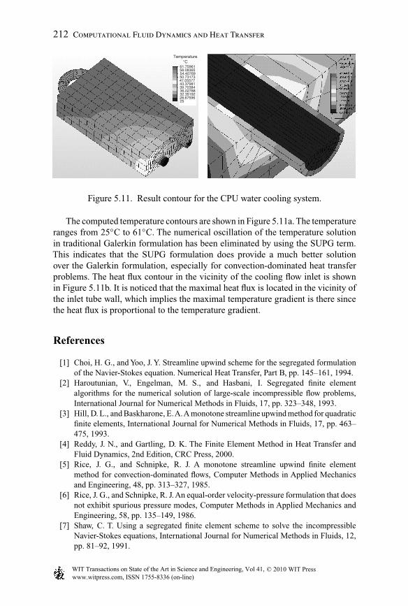
Sunden CH005.tex 10/9/2010 15: 0 Page 212
212 Computational Fluid Dynamics and Heat Transfer
Temperature°C
61.7596158.0836554.4076950.7317347.0557743.3798139.7038436.0278832.3519228.6759625
Figure 5.11. Result contour for the CPU water cooling system.
The computed temperature contours are shown in Figure 5.11a. The temperatureranges from 25◦C to 61◦C. The numerical oscillation of the temperature solutionin traditional Galerkin formulation has been eliminated by using the SUPG term.This indicates that the SUPG formulation does provide a much better solutionover the Galerkin formulation, especially for convection-dominated heat transferproblems. The heat flux contour in the vicinity of the cooling flow inlet is shownin Figure 5.11b. It is noticed that the maximal heat flux is located in the vicinity ofthe inlet tube wall, which implies the maximal temperature gradient is there sincethe heat flux is proportional to the temperature gradient.
References
[1] Choi, H. G., and Yoo, J. Y. Streamline upwind scheme for the segregated formulationof the Navier-Stokes equation. Numerical Heat Transfer, Part B, pp. 145–161, 1994.
[2] Haroutunian, V., Engelman, M. S., and Hasbani, I. Segregated finite elementalgorithms for the numerical solution of large-scale incompressible flow problems,International Journal for Numerical Methods in Fluids, 17, pp. 323–348, 1993.
[3] Hill, D. L., and Baskharone, E.A.A monotone streamline upwind method for quadraticfinite elements, International Journal for Numerical Methods in Fluids, 17, pp. 463–475, 1993.
[4] Reddy, J. N., and Gartling, D. K. The Finite Element Method in Heat Transfer andFluid Dynamics, 2nd Edition, CRC Press, 2000.
[5] Rice, J. G., and Schnipke, R. J. A monotone streamline upwind finite elementmethod for convection-dominated flows, Computer Methods in Applied Mechanicsand Engineering, 48, pp. 313–327, 1985.
[6] Rice, J. G., and Schnipke, R. J. An equal-order velocity-pressure formulation that doesnot exhibit spurious pressure modes, Computer Methods in Applied Mechanics andEngineering, 58, pp. 135–149, 1986.
[7] Shaw, C. T. Using a segregated finite element scheme to solve the incompressibleNavier-Stokes equations, International Journal for Numerical Methods in Fluids, 12,pp. 81–92, 1991.
www.witpress.com, ISSN 1755-8336 (on-line) WIT Transactions on State of the Art in Science and Engineering, Vol 41, © 20 WIT Press10

Sunden CH005.tex 10/9/2010 15: 0 Page 213
Equal-order segregated finite-element method 213
[8] Schunk, P. R., and Heroux, M. A. Iterative solvers and preconditioners for fully-coupled finite element formulations of incompressible fluid mechanics and relatedtransport problems, Sandia National Laboratories, Albuquerque, New Mexico, 87185–0835, 2001.
[9] Tezduyar, T., and Sathe, S. Stabilization parameters in SUPG and PSPG formulations,Journal of Computational and Applied Mechanics, 4(1), pp. 71–88, 2003.
[10] du Toit, C. G. A segregated finite element solution for non-isothermal flow, ComputerMethods in Applied Mechanics and Engineering, 182(3), pp. 457–481(25), 2000.
[11] Van Zijl, and du Toit, C. G. A SIMPLEST finite element solution of the incompress-ible Navier-Stokes equations, In: Proc. Symposium of Finite Element Method, SouthAfrica, 1992.
[12] Vellando, P. On the resolution of the viscous incompressible flow for various SUPGfinite element formulations, European congress on the Computational Methods in theApplied Sciences and Engineering – (ECCOMAS) 2000, Barcelona, 2000.
[13] Wang, G. A fast and robust variant of the simple algorithm for finite-element sim-ulations of incompressible flows, Computational Fluid and Solid Mechanics, 2,pp. 1014–1016, Elsevier, 2001.
[14] Wang, G. A conservative equal order finite element method using the collo-cated GALERKIN approach, 8th AIAA/ASME Thermo-physics and heat transferconference, St. Louis, Missouri, AIAA 2002-3206, 2001.
[15] Wansophark, N. Enhancement of segregated finite element method with adaptivemeshing technique for viscous incompressible thermal flow analysis, Science Asia.29(2), pp. 155–162, 2003.
[16] Xie, J. Equal-order segregated finite element formulation for flow and phase changeproblems, Doctoral Dissertations, University of Wisconsin, 2007.
www.witpress.com, ISSN 1755-8336 (on-line) WIT Transactions on State of the Art in Science and Engineering, Vol 41, © 20 WIT Press10