OOpen Pi

Pue

it Quar

Proj

DeparUn

erto Rico WatUn

4th Qu

ry Resto

ject Year: Ma

Sub

SangchAssoc

rtment of Civiniversity of P

Su

er Resources niversity of P

Febr

uarterly Rep

oration

r. 1, 2008 ~ F

bmitted by:

hul Hwang, Phciate Professoil Engineeringuerto Rico at

bmitted to:

and Environmuerto Rico at

uary 28, 2009

ort

n to Bio‐

Feb. 28, 2009

hD or g and Surveyin

Mayaguez

mental Resea Mayaguez

9

‐Viable

ng

arch Institute

Land

2

Table of Contents List of Tables ................................................................................................................................................. 3

List of Figures ................................................................................................................................................ 4

List of Photos ................................................................................................................................................. 5

Introduction .................................................................................................................................................. 6

Materials ....................................................................................................................................................... 6

Experimental Methods ................................................................................................................................. 7

Water Quality Assessment ........................................................................................................................ 7

3‐Factor, 2‐Level Statistical Design and Analysis .................................................................................. 7

Preliminary Leaching Test for Each Solid Components ......................................................................... 9

Long‐Term Water Quality Monitoring 1: Temperature Effect ............................................................ 10

Long‐Term Water Quality Monitoring 2: Amendment Effect ............................................................. 11

Bio‐viability Assessment ......................................................................................................................... 12

Germination with CAA Water ............................................................................................................. 12

Multifactor Assessment on Germination and Growth........................................................................ 12

Potential Effect of Physical Hindrance by CAA Layer .......................................................................... 13

Effect of Hardness in Water ................................................................................................................ 14

Expansion of Assessment of Physical Hindrance with Various Plants ................................................ 15

Analysis ....................................................................................................................................................... 15

Results and Discussion ................................................................................................................................ 16

Water Quality Assessment ...................................................................................................................... 16

3‐Factor, 2‐Level Statistical Analysis ................................................................................................... 18

Preliminary Leaching Test for Individual Solid Components .............................................................. 24

Long‐Term Water Quality Monitoring 1: Temperature Effect ............................................................ 26

Long‐Term Water Quality Monitoring 2: Effect of Compositions ....................................................... 26

Bio‐viability Assessment ......................................................................................................................... 27

Germination in a Worst Case Scenario ............................................................................................... 27

Germination and Growth Assessment with Multiple Factors ............................................................ 27

Physical Hindrance .............................................................................................................................. 29

Effect of Hardness ............................................................................................................................... 32

Expansion of Physical Hindrance Experiment with Various Plants ..................................................... 33

On‐going and Future Studies ...................................................................................................................... 38

3

Result Disseminations ................................................................................................................................. 39

References .................................................................................................................................................. 39

List of Tables Table 1. 3‐factor, 2‐level statistical design matrix. ....................................................................................... 9 Table 2. Design matrix of preliminary leaching test for each solid material. ............................................. 10 Table 3. Soils and CAA distribution of two identical columns used for Long‐Term Water Quality

Monitoring 1: Temperature effect. ................................................................................................ 10 Table 4.Soils and CAA distribution of the column reactor used for Long‐Term Water Quality Monitoring 2:

Amendment effect. ........................................................................................................................ 11 Table 5. Initial germination experiment matrix where water infiltrated from the CAAs column was

sprayed to the reactors. ................................................................................................................. 12 Table 6. Design matrix to assess the effects of multiple factors on the germination rate and growth. .... 13 Table 7. Specifications of the reactors run for testing physical hindrance of the CAA against germination

and growth. .................................................................................................................................... 14 Table 8. Design of the experiment to assess the effect of hardness on germination and growth. ............ 15 Table 9. Water infiltration ratio and water retention capacity of each column packed with different solid

materials. ....................................................................................................................................... 24 Table 10. Results of analysis on pH, specific conductivity and hardness of rain and tap waters (two

samples each). ............................................................................................................................... 29

4

List of Figures Figure 1. Schematic of backfilling of the site. ............................................................................................... 8 Figure 2. Schematics of column set‐up for Long‐Term Water Quality Monitoring. ................................... 11 Figure 3. Schematics of the reactors run for testing physical hindrance of the CAA against germination

and growth. .................................................................................................................................... 14 Figure 4. Assessment of CAAs as a nutrient source for the various plants: botellas, papayas, beans and

pumpkins. ....................................................................................................................................... 15 Figure 5. Volume of water infiltrated weekly in each reactor. ................................................................... 16 Figure 6. Value of pH in the water infiltrated weekly in each reactor. ....................................................... 17 Figure 7. Turbidity in the water infiltrated weekly from each reactor. ...................................................... 17 Figure 8. Specific conductivity in the water infiltrated weekly from each reactor..................................... 18 Figure 9. Examples of the statistical analysis using the Minitab software. ................................................ 19 Figure 10. Factors and their extent to have produced a statistically significant difference in pH values

(top) and turbidity (bottom). ......................................................................................................... 20 Figure 11. Factors and their extent to have produced a statistically significant difference in hardness. .. 21 Figure 12. Plots of the main effects on the amount of infiltrated water (top row) and pH values (bottom

row). ............................................................................................................................................... 22 Figure 13. Plots of the main effects on the amount of turbidity (top row) and hardness (bottom row). .. 23 Figure 14. Volume of water collected from each reactor. .......................................................................... 24 Figure 15. Trends of pH (top) and turbidity (bottom) in the infiltrated water collected. .......................... 25 Figure 16. Results of the effects of multiple factors on the product of germination rate and shoot length. .................................................................................................................................................................... 28 Figure 17. Height of 6 shoots germinated from each pot. 3 shoots, 1 shoot and 3 shoots did not survive

after about a month of growth in the Reactor 1, 2 and 4, respectively. ....................................... 30 Figure 18. Results of the study which aimed to assess effect of physical hindrance on germination and

growth. ........................................................................................................................................... 31 Figure 19. Length of bean shoots when receiving water at different hardness concentrations. Bars

indicate standard deviations: n=3 for the reactors receiving 0, 4, 20, and 40 mg/L hardness as CaCO3, whereas n=4 for 80 mg/L case. .......................................................................................... 32

Figure 20. The numbers of bean leaves when receiving water at different hardness concentrations. Bars indicate standard deviations: n=3 for the reactors receiving 0, 4, 20, and 40 mg/L hardness as CaCO3, whereas n=4 for 80 mg/L case. .......................................................................................... 33

Figure 21. Height of shoots and the numbers of leaves of papayas. .......................................................... 34 Figure 22. Chlorophyll intensity in the papaya leaves. ............................................................................... 35 Figure 23. Height of shoots (top) and the numbers of leaves (bottom) of the beans. ............................... 36 Figure 24. The numbers (top) and length (bottom) of bean sacks. ............................................................ 37 Figure 25. The numbers of pumpkin leaves. ............................................................................................... 38

5

List of Photos Photo 1. Soil Sampling on site. ...................................................................................................................... 6 Photo 2. Coal ash aggregates before (left) and after (right) preparation for the experiment, .................... 7 Photo 3. Column Reactors setup for water quality assessment in a statistical design and analysis. ........... 8 Photo 4. Views of leaching tests of each solid material used in the project. ............................................... 9 Photo 5. Column set up for the experiment of water quality assessment with the worst‐case

combinational refilling and temperature effect. ........................................................................... 26 Photo 6. Column set up for the experiment of water quality assessment with the best‐case

combinational refilling. .................................................................................................................. 26 Photo 7. Germination results of bean (top row) and pumpkin (bottom row) seeds. ................................ 27 Photo 8. Beans and pumpkins growing in various reactors which were designed to assess the effects of

multiple factors on the germination rate and shoot growth. ........................................................ 28 Photo 9. Scene of the 1st day (left) and the 20th day (right) of the reactors to assess physical hindrance of

the CAAs. ........................................................................................................................................ 29 Photo 10. Resulting view of the experiment to assess the effect of hardness on germination and growth. .................................................................................................................................................................... 32 Photo 11. Various plants (botellas, beans, papayas, and pumpkins) tested for potential physical

hindrance. ...................................................................................................................................... 33 Photo 12. Comparison of the growth of botellas between the initial day (left) and 160th day later (right). .................................................................................................................................................................... 34

6

Introduction As the magnitude of civil, transportation and construction infrastructure has expanded since the industrial revolution, demands for construction‐grade sand and gravel has subsequently increased. These row materials are heavily being exploited in PR today and used for concrete, general fill, and road subgrade material, bridges, airports, road surfacing, and aqueduct and sewer systems. Resulting open pit, in turn, may adversely affect health and safety of human beings if not appropriately managed or restored (MDNR, 1992). The main goal of this study is to investigate the feasibility of coal combustion ash aggregates (CAA)‐based refill for the open pits in Santa Isabel. The site is planned to be used as an agricultural land after restoration. Therefore, this study aims to assess the potential risks in relation to contamination of soil and groundwater associated with the use of industrial byproducts CAAs. Another objective is to evaluate bio‐viability on the land after restoration. To meet this end, laboratory feasibility tests and computational modeling were initially proposed to perform for the period of 2 years.

Materials The open pit site was filled with the dredged sandy sediments from the Guayama bay on the bottom at a depth of 0.3 m. As the site will be eventually used as an agricultural area, an organic‐rich soil from the Coamo Lake will be used as a top soil at a depth of 1 m. In these regards, two soils were sampled on site as shown in Photo 1. After being transported, the soil samples passed a sieve size 3/8” were collected for the experiment.

Photo 1. Soil Sampling on site.

7

Coal ash aggregates were obtained from a local coal burning power plant in Guayama, PR. It is a solidified mixture of fly and bottom ashes with water. Main chemical components, by weight, are: 51% of (SiO2 + Al2O3 + Fe2O3), 30% Lime (CaO), and 15% SO3 (Pando and Hwang, 2006). The CAAs were first oven dried at 105oC overnight, crushed with a mechanical mixer, and sieved to collect the CAA sizes of 2.36 ~ 9.53 mm (Photo 2).

Photo 2. Coal ash aggregates before (left) and after (right) preparation for the experiment,

Experimental Methods

Water Quality Assessment

3-Factor, 2-Level Statistical Design and Analysis As shown in Figure 1, initial focus was given to the volume of CAAs that can be utilized as a substitute subsoil material. For this, as shown in Photo 3, PVC column reactors (3‐in dia. and 30‐in long) were designed, performed, and analyzed by a statistical design with three factors containing two levels each for the assessment of the unsaturated‐zone fate and transport phenomena (Table 1). The volumetric ratio of the CAAs to the organic top soil is a treatment factor with two levels of 8:4 and 4:8, which was the ratio of the depth of the top soil to the CAAs. Simulated precipitation was made three times a week by spraying tap water on the top of the reactors. Precipitation rates are another treatment factor with two different levels: high rainfall 60 mL each application, low rainfall 30 mL each application. Two rainfall amounts were calculated according to the actual maximum and minimum average precipitation in Santa Isabel. Half of the reactors were assigned to the smaller particle sizes (2.36 ~ 4.75 mm) of CAAs and the remainder to the greater particle sizes (4.75 ~ 9.53 mm). Thus, the particle size of the CAAs is another treatment factor containing two levels.

8

Figure 1. Schematic of backfilling of the site.

Photo 3. Column Reactors setup for water quality assessment in a statistical design and analysis.

Sandy Bottom Soil from Guayama Bay

Organic Top Soil from Coamo Lake

Santa Isabel Site Soil 20 ~ 60 m

GWT

3 m

0.3 m

Coal Ash Aggregates

9

Table 1. 3‐factor, 2‐level statistical design matrix.

Preliminary Leaching Test for Each Solid Components Total 8 plastic reactors (2.5‐in D x 6‐in L) were constructed to test leaching characteristics of each solid material being used in the project as shown in Photo 4. Each component was packed at a depth of 5 inches. Table 2 shows the design matrix of leaching test. Tap water was sprayed on the top of the reactors on every Mondays, Wednesdays, and Fridays. During the first 2 watering events, 40 mL was sprayed, but the amount of water added was increased to 100 mL to collect enough amount of infiltrated water with which water quality parameters were analyzed. This experiment was done over 4 weeks.

Photo 4. Views of leaching tests of each solid material used in the project.

Reactors Top Soil (in) CCPs (in) Bottom Soil (in) Site Soil (in) CCPs Size Rain IntensityR1 8 4 4 10 A HighR2 8 4 4 10 A HighR3 8 4 4 10 A LowR4 8 4 4 10 A LowR5 8 4 4 10 B HighR6 8 4 4 10 B HighR7 8 4 4 10 B LowR8 8 4 4 10 B LowR9 4 8 4 10 A HighR10 4 8 4 10 A HighR11 4 8 4 10 A LowR12 4 8 4 10 A LowR13 4 8 4 10 B HighR14 4 8 4 10 B HighR15 4 8 4 10 B LowR16 4 8 4 10 B Low

10

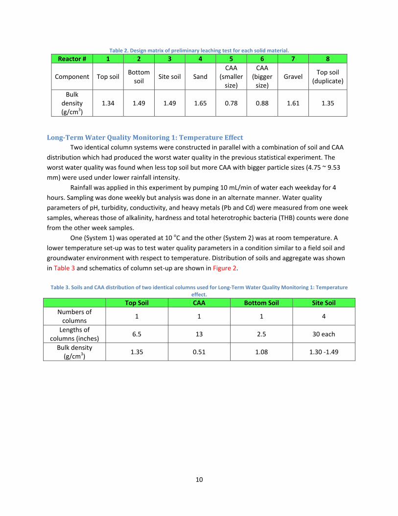
Table 2. Design matrix of preliminary leaching test for each solid material.

Reactor # 1 2 3 4 5 6 7 8

Component Top soil Bottom

soil Site soil Sand

CAA (smaller

size)

CAA (bigger

size) Gravel

Top soil (duplicate)

Bulk density (g/cm3)

1.34 1.49 1.49 1.65 0.78 0.88 1.61 1.35

Long-Term Water Quality Monitoring 1: Temperature Effect Two identical column systems were constructed in parallel with a combination of soil and CAA distribution which had produced the worst water quality in the previous statistical experiment. The worst water quality was found when less top soil but more CAA with bigger particle sizes (4.75 ~ 9.53 mm) were used under lower rainfall intensity.

Rainfall was applied in this experiment by pumping 10 mL/min of water each weekday for 4 hours. Sampling was done weekly but analysis was done in an alternate manner. Water quality parameters of pH, turbidity, conductivity, and heavy metals (Pb and Cd) were measured from one week samples, whereas those of alkalinity, hardness and total heterotrophic bacteria (THB) counts were done from the other week samples. One (System 1) was operated at 10 oC and the other (System 2) was at room temperature. A lower temperature set‐up was to test water quality parameters in a condition similar to a field soil and groundwater environment with respect to temperature. Distribution of soils and aggregate was shown in Table 3 and schematics of column set‐up are shown in Figure 2.

Table 3. Soils and CAA distribution of two identical columns used for Long‐Term Water Quality Monitoring 1: Temperature effect.

Top Soil CAA Bottom Soil Site Soil Numbers of

columns 1 1 1 4

Lengths of columns (inches)

6.5 13 2.5 30 each

Bulk density (g/cm3)

1.35 0.51 1.08 1.30 ‐1.49

11

Figure 2. Schematics of column set‐up for Long‐Term Water Quality Monitoring. The System 1 was constructed in the same way as the System 2, except for the operating temperature. It was coiled with a vinyl tube and cold water (10oC) was recirculated through it by a temperature controlled bath. The columns and coiled tubes were wrapped with an insulation sheet. Tap water was pumped to the Systems 1 and 2 at a rate of 10 mL/min from a reservoir by a peristaltic pump. Pumping was scheduled for 3 hours per week day at the consistent time frame using a timer. Samples were collected from the sampling ports once every two weeks and analyzed for water quality parameters.

Long-Term Water Quality Monitoring 2: Amendment Effect Another column system was constructed with a combination of soil and CAA distribution which had produced the best water quality from the previous statistical experiment. The best water quality was measured when more top soil but less CAA with smaller particle sizes (2.36 ~ 4.75 mm) were tested under greater rainfall intensity (20 mL/min). The same rainfall frequency that was used for the Long‐Term Water Quality Monitoring 1 was used for this experiment. Sampling and analysis schemes were the same as the previous experiment. Distribution of soils and aggregate was shown in Table 4. Table 4.Soils and CAA distribution of the column reactor used for Long‐Term Water Quality Monitoring 2: Amendment effect.

Top Soil CAA Bottom Soil Site Soil Numbers of

columns 1 1 1 4

Lengths of columns (inches)

13 6.5 2.5 30 each

Bulk density (g/cm3)

1.32 0.53 1.08 1.32

Top soil column CAA column Bottom soil column Site soil columns Pump Sampling points

12

Bio-viability Assessment

Germination with CAA Water Germination of bean and pumpkin seeds was assessed in a worst case scenario that the plants might get experienced due to the presence of the CAAs. A hypothesis was that no toxic chemicals from the CAAs, if any, would be taken up by the plants so that seeds would germinate and grow. For this, water infiltrated from the CAAs was collected from a separate column system. In the flat‐bottom, porcelain funnel (6‐in dia. and 8‐in long), 1,080 g of CAAs were layered on the top of 835 g of gravels. 1,500 g of sand covered the CAAs layer. Both clean gravels and sands were used as supporting layers to facilitate the hydraulics of water. Total 3 L of tap water was poured to the column and infiltrated water was collected and used for spraying to the reactors prepared as shown in Table 5.

Table 5. Initial germination experiment matrix where water infiltrated from the CAAs column was sprayed to the reactors.

Reactors Gravel (grams) Nominal depth: 2.5 inches

Top Soil (grams) Nominal depth: 6.5 inches

Seeds

1 201 1262 Beans 2 202 1264 Beans 3 200 1270 Pumpkin 4 196 1262 Pumpkin

Four reactors (4‐in dia. and 11‐in length) were put in an environmental chamber which controlled temperature at 30 oC with a refrigerated and heating bath circulator (Thermo NESLAB RTE‐10 Digital One ). The chamber was also equipped with a 20 W lighting system (GRO‐LUX, Sylvania) which was scheduled to turn on from 1 pm to 10 pm with a timer. The infiltrated water collected from the CAA column was sprayed on every other day at an amount of 105 mL which was calculated according to the actual maximum average precipitation in Santa Isabel. This germination experiment was performed for 2 weeks.

Multifactor Assessment on Germination and Growth Another germination experiment was conducted after the first germination experiment aforementioned. This time, multiple factors were assessed on their effects on the germination rate and growth. The parameter monitored is the product of the germination rate and shoot growth. First factor evaluated was a backfilling mode with a mixed or a layered application of the top soils and CAAs. Second factor was the type of seeds, bean or pumpkin. Third factor assessed was the ratio of the top soil to the CAAs. Lastly, the type of water sprayed to the systems was tested with natural rain water collected and tap water. Sixteen treatments and 4 control reactors were constructed as shown in Table 6. Plastic reactors were dimensioned with 2.5‐in dia. and 6‐in long. Five seeds were placed to each reactor at a depth of 1.5 inches below surface. Like the previous germination experiments, the reactors were put in the environmental chamber. Corresponding to the actual maximum average precipitation in Santa Isabel, 40 mL of water (rain water or tap water) was sprayed on every other day for 2 weeks.

13

Table 6. Design matrix to assess the effects of multiple factors on the germination rate and growth.

Reactors Mixed/Layered Type of

seed Distribution Type of water

Top Soil (g)

Aggregate (g)

R1 Layered beans 4" top soil+2" aggregate RW 440.1 134.3 R2 Layered beans 2" top soil+4" aggregate TW 225.1 254.3

R3 Mixed beans 66.7% top soil+ 33.3% aggregate RW 445.2 127.7

R4 Mixed beans 33.3% top soil+ 66.7% aggregate TW 222.7 258.6

R5 Layered beans 4" top soil+2" aggregate TW 439.6 134.5 R6 Layered beans 2" top soil+4" aggregate RW 227.5 254.5

R7 Mixed beans 66.7% top soil+ 33.3% aggregate TW 444.5 129.5

R8 Mixed beans 33.3% top soil+ 66.7% aggregate RW 222.5 259.5

R9 Layered pumpkin 4" top soil+2" aggregate RW 439.4 134.5 R10 Layered pumpkin 2" top soil+4" aggregate TW 227.5 254.5

R11 Mixed pumpkin 66.7% top soil+ 33.3% aggregate RW 444.4 129.5

R12 Mixed pumpkin 33.3% top soil+ 66.7% aggregate TW 222.3 256.5

R13 Layered pumpkin 4" top soil+2" aggregate TW 439.6 134.5 R14 Layered pumpkin 2" top soil+4" aggregate RW 227.5 254.5

R15 Mixed pumpkin 66.7% top soil+ 33.3% aggregate TW 447.2 129.5

R16 Mixed pumpkin 33.3% top soil+ 66.7% aggregate RW 222.9 262.5

Reactors Mixed/Layered Type of

seed Distribution Type of water

Top Soil (g)

Aggregate (g)

CR1 N/A beans 6" top soil RW 664.9 / CR2 N/A beans 6" top soil TW 674 / CR3 N/A pumpkin 6" top soil RW 657.6 / CR4 N/A pumpkin 6" top soil TW 677.3 /

Potential Effect of Physical Hindrance by CAA Layer An experiment was conducted to assess potential physical hindrance of the CAAs against seeds germination and growth. In order to accommodate more numbers of the seeds (bean), 4 rectangular reactors were constructed of acrylic plates with effective volume of 800 in3 (13 W x 8 L x 8 D). All 4 reactors had a supporting gravel layer of 2 in on the bottom. The reactors were packed as shown in the following Table 7 and Figure 3.

14

Table 7. Specifications of the reactors run for testing physical hindrance of the CAA against germination and growth.

Layers Reactor 1 Reactor 2 Reactor 3 Reactor 4

Top soil layer Depth (in) 8 6 5 4 Bulk density (g/cm3) 1.51 1.56 1.23 1.56

Hindrance Layer

CAA, depth (in) ‐ 2 1 ‐ Bulk density (g/cm3) ‐ 0.80 0.91 ‐ Gravel, depth (in) ‐ ‐ 2 6 Bulk density (g/cm3) 1.77 1.40

Figure 3. Schematics of the reactors run for testing physical hindrance of the CAA against germination and growth.

Six bean seeds were planted in each reactor at a depth of 1.5 inches. Corresponding to the actual maximum average precipitation in Santa Isabel, 840 mL of tap water was evenly sprayed on the top of the reactors every other day for over 5 weeks. Germination and growth monitoring was done every Mondays and Fridays.

Effect of Hardness in Water An experiment was conducted to elucidate potential contribution of hardness to germination and growth. This experiment was initiated based on the results from the multiple factor germination experiments where the tap water (64.4 mg/L Hardness as CaCO3) spraying showed better germination and growth compared to the rain water (6.3 mg/L Hardness as CaCO3) spraying. Plastic reactors used for the multiple factor experiments (2.5‐in dia. and 6‐in long.) were filled with the organic top soil at a depth of 5 inches. Two seeds were placed to each reactor at a depth of 1.5 inches below surface. Each system was run in duplicate. Corresponding to the actual maximum average precipitation in Santa Isabel, 40 mL of hardness water (0 to 80 mg/L Hardness as CaCO3) was sprayed on every other day for a month. Table 8 shows the design of the experiment.

15

Table 8. Design of the experiment to assess the effect of hardness on germination and growth.

Reactor A B C D E Hardness in the water sprayed

(mg/L as CaCO3) 0 4 20 40 80

Expansion of Assessment of Physical Hindrance with Various Plants After completing Physical Hindrance experiment, all beans were removed from the reactors and the configurations of the reactors were slightly modified as shown Figure 4. This experiment was to assess potential contribution of the CAAs as nutrient source for the plants. Four different plants were tested: botellas, beans, papayas, and pumpkins. Baby botellas and papayas were obtained from a nursery farm at the site and planted in the reactors #1 and #2, and #3 and #4, respectively. Beans were seeded directly to the reactors #3 and #4. Pumpkins were later seeded to the reactors #3 and #4 after the beans were completed with the experiment and removed from the reactors. Due to deeper and bigger roots, the reactors #1 and #2 had deeper top soils by 40% than the reactor #3 and #4. Like the Physical Hindrance experiment, 840 mL of tap water was evenly sprayed on the top of the reactors every other day during the experiment. Germination and growth monitoring was done every Mondays and Fridays.

Figure 4. Assessment of CAAs as a nutrient source for the various plants: botellas, papayas, beans and pumpkins.

Analysis Heavy metals, lead (Pb) and cadmium (Cd), were monitored with the Leadtrak (HACH) and an ion specific electrode (Orion), respectively. The value of pH was measured with an Orion pH meter. Specific conductivity was analyzed with Orion Specific Conductivity Meter Model 162. Turbidity was measured with LaMotte 2020 Turbidimeter. Hardness was analyzed with an ion specific electrode

R1 R2 R3 R4

Top soil

Aggregate

Gravel

16

(Orion). THB was done by the standard plate count using tryptic soy broth as the growth media and then counted after incubation at 30oC for 72 hrs. For bio‐viability assessment, beans and pumpkins were initially selected as the target plants. Their germination rates and shoot growth were monitored. The former is defined as the ratio of the germination to the numbers of the seeds planted. The latter is defined as the physical height of the shoots above the ground. Two target heavy metals, Pb and Cd, in the plants were also analyzed after the Digesdahl digestion (HACH).

Results and Discussion

Water Quality Assessment The water volume infiltrated in each reactor weekly is shown in Figure 5. Apparently, it seems the rainfall intensity influenced greatly on the infiltrated water volume.

Figure 5. Volume of water infiltrated weekly in each reactor.

The infiltrated water from each reactor containing the CAAs had a slightly basic pH (~8.5) throughout the experiment, as shown in Figure 6. A higher pH of the control reactors was attributed to the characteristics of the sand used for the system.

0

20

40

60

80

100

120

140

160

180

0 10 20 30 40 50 60 70

Volu

me

of w

ater

infil

trat

ed (m

L)

Days

CR

R1

R2

R3

R4

R5

R6

R7

R8

R10

R11

R12

R13

R14

R15

R16

17

Figure 6. Value of pH in the water infiltrated weekly in each reactor.

Turbidity was monitored in the range between 0.5 and 1 NTU, except for a couple of outliers, in the beginning of the experiment. However, it reduced to a value less than 0.5 NTU as shown in Figure 7.

Figure 7. Turbidity in the water infiltrated weekly from each reactor.

7.4

7.6

7.8

8.0

8.2

8.4

8.6

8.8

9.0

0 10 20 30 40 50 60 70

pH

Days

CR

R1

R2

R3

R4

R5

R6

R7

R8

R10

R11

R12

R13

R14

R15

R16

0.0

0.5

1.0

1.5

2.0

2.5

3.0

0 10 20 30 40 50 60 70

Turb

idity

(NTU

)

Days

CR

R1

R2

R3

R4

R5

R6

R7

R8

R10

R11

R12

R13

R14

R15

R16

18

Specific conductivity showed higher strengths in all treatment columns compared to that in the control reactor as shown Figure 8. A similar trend was observed for the hardness concentrations.

Figure 8. Specific conductivity in the water infiltrated weekly from each reactor.

Heavy metal analysis showed no concentrations of Pb and Cd. For Pb, the HACH LeadTrak testing methods can detect Pb as low as 5 µg/L as Pb. For ensuring quality of the measurement, a Cole‐Parmer Pb ion selective electrode was also used for Pb analysis. Its lower limit was 0.2 mg/L. For Cd, both an AA spectrometer and a Cole‐Parmer Cd ion selective electrode with a lower limit of 0.2 mg/L were used for the analysis.

3-Factor, 2-Level Statistical Analysis To evaluate the causes and effects produced by the factors aforementioned in the Method section, 3‐factor, 2‐level statistical analysis was conducted based on the corresponding the statistical design. For this purpose, the latest version of the Minitab software was used. Example plots are shown in Figure 9.

0

2

4

6

8

10

12

14

0 10 20 30 40 50 60 70

Cond

uctiv

ity (m

S/cm

)

Days

CR

R1

R2

R3

R4

R5

R6

R7

R8

R10

R11

R12

R13

R14

R15

R16

19

Figure 9. Examples of the statistical analysis using the Minitab software.

As shown in Figure 8 above, the factors produced different effects on the monitored parameters throughout the experiment (i.e., temporal effects). In this regard, those factors which produced statistically significant difference in the monitored parameters were selected and plotted in order to compare temporal effects of the factors. Figures 10 and 11 show temporally significant factors which produced a statistical difference in pH values (top) and turbidity (bottom,) and hardness, respectively.

20

Figure 10. Factors and their extent to have produced a statistically significant difference in pH values (top) and turbidity

(bottom).

A

A

B B

BB

B

C

CC

CAC

AC

AC AC AC

BC

BC

AB

ABC

ABC

0

5

10

15

20

25

7 9 14 18 25 30 35 39 44 49 53 60 63

Stan

dard

ized

effe

cts

Days

A

B

C

AC

BC

AB

ABC

A A

B

BB

C

C

CC

CAC

AC

BC

BC BC

BC

AB

ABC

ABCABC

0

5

10

15

20

25

7 9 14 18 25 30 35 39 44 49 53 60 63

Stan

dard

ized

effe

cts

Days

A

B

C

AC

BC

AB

ABC

21

Figure 11. Factors and their extent to have produced a statistically significant difference in hardness.

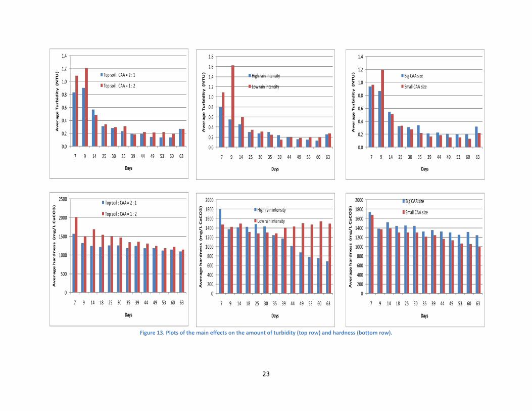
For better understanding of statistically significant effects that were produced by the main factors, plots containing only the main effects and causes were constructed as shown in Figures 12 and 13. The rainfall intensity undoubtedly significantly influenced on the amount of the infiltrated water as shown in Figure 12. The difference in the amount of the infiltrated water was all statistically different, with the greater rainfall intensity being produced more amount of the infiltrated water. For the values of pH, significantly higher pH values were observed for the reactors with low‐level rainfall intensities and small‐sized CAAs. As shown in Figure 13, turbidity was statistically higher for the reactors with low‐level rainfall intensities, more CAAs ratio, and smaller size CAAs. However, in the later part of the experiment, the infiltrated water from the bigger size CAAs produced significantly higher turbidity. Statistically higher hardness concentrations were monitored for the reactors with more CAAs ratio up to the middle of the experiment. However, low‐level rainfall intensity dominantly produced significantly higher concentrations of hardness in the later experiment.

AA

A A

A AA

B BB

BB

B

B

B

B

C C CAC

AC

ACAC

ACBCBC BC BC

ABC

0

5

10

15

20

25

7 9 14 18 25 30 35 39 44 49 53 60 63

Stan

dard

ized

effe

cts

Days

A

B

C

AC

BC

AB

ABC

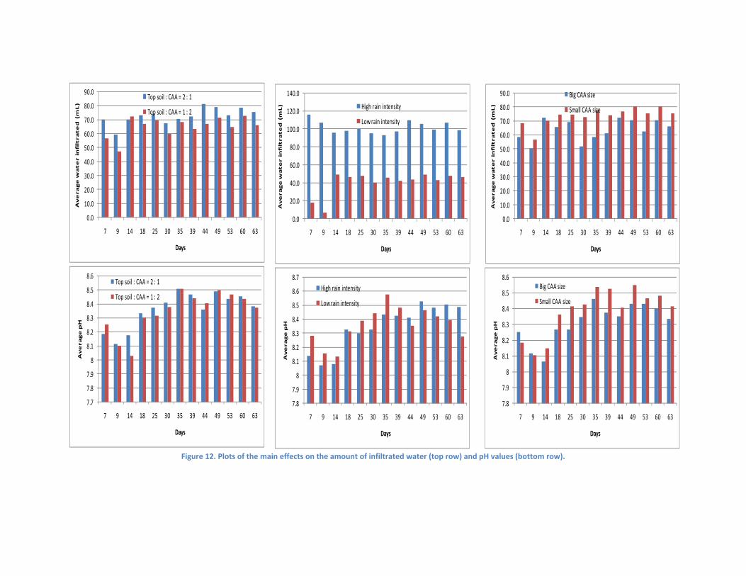
Figure 12. Plots of the main effects on the amount of infiltrated water (top row) and pH values (bottom row).

0.0

10.0

20.0

30.0

40.0

50.0

60.0

70.0

80.0

90.0

7 9 14 18 25 30 35 39 44 49 53 60 63

Av

era

ge

wa

te

r i

nfi

ltra

te

d (

mL

)

Days

Top soil : CAA = 2 : 1

Top soil : CAA = 1 : 2

0.0

20.0

40.0

60.0

80.0

100.0

120.0

140.0

7 9 14 18 25 30 35 39 44 49 53 60 63

Av

era

ge

wa

te

r i

nfi

ltra

te

d (

mL

)

Days

High rain intensity

Low rain intensity

0.0

10.0

20.0

30.0

40.0

50.0

60.0

70.0

80.0

90.0

7 9 14 18 25 30 35 39 44 49 53 60 63

Av

era

ge

wa

te

r i

nfi

ltra

te

d (

mL

)

Days

Big CAA size

Small CAA size

7.8

7.9

8

8.1

8.2

8.3

8.4

8.5

8.6

8.7

7 9 14 18 25 30 35 39 44 49 53 60 63

Av

era

ge

pH

Days

High rain intensity

Low rain intensity

7.8

7.9

8

8.1

8.2

8.3

8.4

8.5

8.6

7 9 14 18 25 30 35 39 44 49 53 60 63

Av

era

ge

pH

Days

Big CAA size

Small CAA size

7.7

7.8

7.9

8

8.1

8.2

8.3

8.4

8.5

8.6

7 9 14 18 25 30 35 39 44 49 53 60 63

Av

era

ge

pH

Days

Top soil : CAA = 2 : 1

Top soil : CAA = 1 : 2

23

Figure 13. Plots of the main effects on the amount of turbidity (top row) and hardness (bottom row).

0.0

0.2

0.4

0.6

0.8

1.0

1.2

1.4

7 9 14 25 30 35 39 44 49 53 60 63

Av

era

ge

Tu

rb

idit

y (N

TU

)

Days

Top soil : CAA = 2 : 1

Top soil : CAA = 1 : 2

0.0

0.2

0.4

0.6

0.8

1.0

1.2

1.4

1.6

1.8

7 9 14 25 30 35 39 44 49 53 60 63

Av

era

ge

Tu

rb

idit

y (N

TU

)

Days

High rain intensity

Low rain intensity

0.0

0.2

0.4

0.6

0.8

1.0

1.2

1.4

7 9 14 25 30 35 39 44 49 53 60 63

Av

era

ge

Tu

rb

idit

y (N

TU

)

Days

Big CAA size

Small CAA size

0

200

400

600

800

1000

1200

1400

1600

1800

2000

7 9 14 18 25 30 35 39 44 49 53 60 63

Av

era

ge

ha

rd

ne

ss (m

g/

L C

aC

O3

)

Days

High rain intensity

Low rain intensity

0

200

400

600

800

1000

1200

1400

1600

1800

2000

7 9 14 18 25 30 35 39 44 49 53 60 63

Av

era

ge

ha

rd

ne

ss (m

g/

L C

aC

O3

)

Days

Big CAA size

Small CAA size

0

500

1000

1500

2000

2500

7 9 14 18 25 30 35 39 44 49 53 60 63

Av

era

ge

ha

rd

ne

ss (m

g/

L C

aC

O3

)

Days

Top soil : CAA = 2 : 1

Top soil : CAA = 1 : 2

Preliminary Leaching Test for Individual Solid Components Figure 14 shows the trends of water infiltration for each column packed with the different solid materials (i.e., top soil, bottom soil, site soil, sand, small CAA, big CAA, and gravel). A steady‐state water infiltration was calculated by using infiltration volume data after total 120 mL was added to each column. After that event, the infiltration trend reached a pseudo plateau producing a constant amount of water. Results are sown in Table 9. With those infiltration ratio data, water retention capacity at a steady‐state was calculated per grams of solid materials tested.

Figure 14. Volume of water collected from each reactor.

Table 9. Water infiltration ratio and water retention capacity of each column packed with different solid materials.

Solid Type Top soil

1 Bottom

soil Site soil Sand

CAA small

CAA big

Gravel Top

soil 2 Steady‐state Water Infiltration Ratio (%)

70.6 68.4 72.9 73.7 83.5 83.2 88.9 73.3

Water Retention (mL H2O/g solid)

0.131 0.114 0.121 0.111 0.267 0.236 0.137 0.135

In addition, several water quality parameters were monitored. The values of pH were ranged between 7.5 and 8.5 as shown in Figure 15 (top). Turbidity was also monitored. Interestingly, the bottom and site soils were the most influencing solids which exerted abnormally high turbidity during

0

10

20

30

40

50

60

70

80

90

100

0 100 200 300 400 500 600 700 800 900

Volu

me

of w

ater

col

lect

ed (m

L)

Accumulative volume of water added (mL)

TS‐1

BS

SS

Sand

CAA small

CAA big

Gravel

TS‐2

25

the infiltration test as shown in Figure 15 (bottom). Further sophisticated experiment is warranted to assess the contribution extent of each solid material to overall water quality parameters.

Figure 15. Trends of pH (top) and turbidity (bottom) in the infiltrated water collected.

7.0

7.5

8.0

8.5

9.0

0 5 10 15 20 25 30 35

pH

Time (days)

top soil1 bottom soil site soil sand

CAA small CAA big gravel top soil2

0

20

40

60

80

100

0 5 10 15 20 25 30 35

Turb

idit

y (N

TU)

Time (days)

TS1

BS

SS

SAND

CAA small

CAA big

GRAVEL

TS2

26

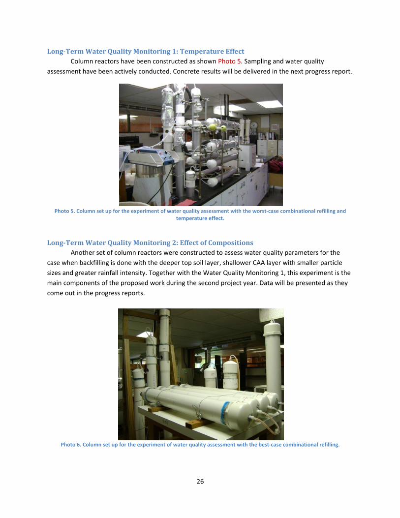
Long-Term Water Quality Monitoring 1: Temperature Effect Column reactors have been constructed as shown Photo 5. Sampling and water quality assessment have been actively conducted. Concrete results will be delivered in the next progress report.

Photo 5. Column set up for the experiment of water quality assessment with the worst‐case combinational refilling and

temperature effect.

Long-Term Water Quality Monitoring 2: Effect of Compositions Another set of column reactors were constructed to assess water quality parameters for the case when backfilling is done with the deeper top soil layer, shallower CAA layer with smaller particle sizes and greater rainfall intensity. Together with the Water Quality Monitoring 1, this experiment is the main components of the proposed work during the second project year. Data will be presented as they come out in the progress reports.

Photo 6. Column set up for the experiment of water quality assessment with the best‐case combinational refilling.

27

Bio-viability Assessment

Germination in a Worst Case Scenario It was hypothesized that neither toxic chemicals would be leached out of the CAAs nor the plants would take up them, if any, so that the seeds would germinate and the plants would grow. To test this hypothesis, water collected form a column filled with the CAAs was sprayed to the seeds as a worst case scenario and their germination was monitored. As shown in Photo 7, both beans and pumpkins germinated and grew in a good shape. After 2 weeks, roots, leaves and stems of both plants were analyzed with respect to the target heavy metals, Pb and Cd. Both heavy metals were not detected.

Photo 7. Germination results of bean (top row) and pumpkin (bottom row) seeds.

Germination and Growth Assessment with Multiple Factors Generally, beans germinated and grew much better than pumpkins during the period of the experiment (2 weeks) as shown in Photo 8 and Figure 17. Between two backfilling modes, a layered mode showed better results than a mixed mode. Regardless of the seed type, better results were observed with a greater depth of the top soil for a layered backfilling mode and a higher ratio of the top soil to the CAAs for a mixed mode. Both plants also showed better results when their seeds were planted into the system that had more top soils than the CAAs.

28

It was suspected that a physical hindrance due to the presence of the CAAs occurred, thereby poorer germination and growth patterns for the mixed backfilling mode and the more CAA ratio in the layered mode. Additional experiment was conducted to disclose this suspicion.

Photo 8. Beans and pumpkins growing in various reactors which were designed to assess the effects of multiple factors on

the germination rate and shoot growth.

Figure 16. Results of the effects of multiple factors on the product of germination rate and shoot length. When sprayed with the tap water, better germination and growth were observed in comparison to the rain water application. Water quality analysis was done with respect to specific conductivity, pH, and hardness of both waters (Table 10).

0

1

2

3

4

5

6

7

8

4" topsoil 2" topsoil 67% soil 67% CAA more soil more CAA layered mixed rain tap

Layered Mixed Amount Layered/Mixed Water type

Prod

uct o

f sho

ot le

ngth

and

ger

min

atio

n ra

te

Beans Pumpkins

29

Table 10. Results of analysis on pH, specific conductivity and hardness of rain and tap waters (two samples each).

pH Specific Conductivity

(µS/cm) Hardness

(mg/L as CaCO3) Tap water 7.9 ± 0.1 42.6 ± 0.2 64.4 ± 4.0 Rain water 7.5 ± 0.1 37.5 ± 28.1 6.3 ± 0.6

As shown, a major difference between two waters was found in the concentration of hardness, with the tap water being greater 10 times. Additional experiment was performing to elucidate potential contribution of hardness in the tap water which showed better germination and growth compared to the rain water.

Physical Hindrance As shown in Photo 9 and Figure 18, all of 6 bean seeds germinated from each reactor. However, after about a month of growth, 3 shoots died from the Reactors 1 and 4 (i.e., 50% survivability), and 1 shoot died from the Reactor 2 (i.e., 83% survivability). No shoot death was observed from the Reactor 3, resulting in 100% survivability).

Photo 9. Scene of the 1st day (left) and the 20th day (right) of the reactors to assess physical hindrance of the CAAs.

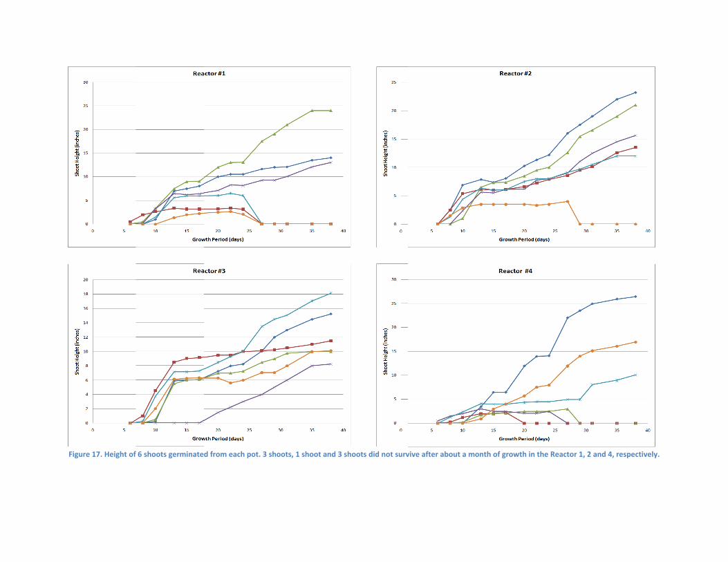
Figure 17. Height of 6 shoots germinated from each pot. 3 shoots, 1 shoot and 3

3 shoots did not survvive after about a moonth of growth in the Reactor 1, 2 and 4,

, respectively.

G3. Both Reinch CAA top soil grweeks of

Figu

enerally, the eactors had tlayer below 5rew a similar growth. How

ure 18. Results o

Reactor 2 hahe CAA layers5‐inch top soimanner that

wever, its grow

of the study whi

ad the best shs: 2‐inch CAAl for the Reacthose in the

wth was limite

ich aimed to ass

hoot growth aA layer below ctor 3. The shReactors 2 aned.

sess effect of ph

as shown Figu6‐inch top so

hoots in the Rnd 3 which ha

hysical hindrance

ure 19, followoil for the ReaReactor 1 whicad the CAA la

e on germinatio

wed by the Reactor 2, wherech had only 8yers up to 3

on and growth.

actor eas 1‐

8‐in

32

Effect of Hardness Reactors in duplicate were sprayed with water having different hardness concentrations (0 ~ 80 mg/L as CaCO3). The Reactors having received the highest hardness water made 100% germination (i.e., 4 germinations out of 4 seeds planted). Other Reactors made 75% (i.e., 3 out 4) germination. As shown in Photo 10 and Figure 20, the highest growth of the beans was achieved in Reactor D which has been sprayed with water at a hardness concentration of 80 mg/L as CaCO3. In general, the numbers of leaves were not significantly different among the reactors (Figure 21).

Photo 10. Resulting view of the experiment to assess the effect of hardness on germination and growth.

Figure 19. Length of bean shoots when receiving water at different hardness concentrations. Bars indicate standard

deviations: n=3 for the reactors receiving 0, 4, 20, and 40 mg/L hardness as CaCO3, whereas n=4 for 80 mg/L case.

0

5

10

15

20

25

0 12 14 16 21 23 29 33 35 37 42 44

Leng

th o

f sho

ots

(inc

hes)

Time (days)

0 mg/L as CaCO3

4 mg/L as CaCO3

20 mg/L as CaCO3

40 mg/L as CaCO3

80 mg/L as CaCO3

33

Figure 20. The numbers of bean leaves when receiving water at different hardness concentrations. Bars indicate standard

deviations: n=3 for the reactors receiving 0, 4, 20, and 40 mg/L hardness as CaCO3, whereas n=4 for 80 mg/L case.

Expansion of Physical Hindrance Experiment with Various Plants As shown in Photo 11, botellas, papayas, beans and later pumpkins were tested with respect to physical hindrance that the CAA layer might exert for their roots and consequently their growth. Baby botellas (~8 inches) and papayas (~5 inches) were planted directly to the Reactors, whereas beans and pumpkins were seeded to the Reactors.

Photo 11. Various plants (botellas, beans, papayas, and pumpkins) tested for potential physical hindrance.

0

2

4

6

8

10

12

14

0 16 23 29 35 44

Num

bers

of L

eave

s

Time (days)

0 mg/L as CaCO3

4 mg/L as CaCO3

20 mg/L as CaCO3

40 mg/L as CaCO3

80 mg/L as CaCO3

34

Botellas: Two identical baby botellas were planted in the Reactor 1 and 2 (Photo 12). Due to the physical characteristics of their leaves, no specific measurements have done with them. However, regardless of the amendments (CAAs vs. gravel) below 7‐in top soil, both botellas have grown well so far up to more than 4 months.

Photo 12. Comparison of the growth of botellas between the initial day (left) and 160th day later (right).

Papayas: Initially, one papaya was planted to each Reactor (Reactors 3 and 4). However, those

two baby papayas died after one month due to parasites developed on the leaves. Four new baby papayas were obtained from a nursery farm and two were planted again to one reactor. This time, a commercial pesticide (VEL 4283) was diluted 130 times as instructed and the leaves were gently swabbed with it. Results are shown in Figure 22.

Figure 21. Height of shoots and the numbers of leaves of papayas.

0

2

4

6

8

10

0

2

4

6

8

10

0 20 40 60 80 100 120 140

Num

bers

of L

eave

s

Hei

ght o

f Sho

ots

(inc

hes)

Time (days)

Reactor 3 (Shoot)

Reactor 4 (Shoot)

Reactor 3 (Leaf)

Reactor 4 (Leaf)

35

As shown, shorter shoots but more leaves were found from the papayas planted in Reactor 3 which had the CAAs layer five inches below the top soil. However, it is not sure at the moment whether or not the initial physical conditions have influenced the results. That is, four identical baby papayas were obtained and planted to the Reactors but the Reactor 3 started with shorter shoot and more leaves in the beginning. A chlorophyll meter (SPAD‐502, Konica Minolta) was acquired in the middle of the experiment and the chlorophyll intensity was monitored on the leaves of papayas. Monitoring results showed a healthier growth of papayas in the Reactor 3 which had a CAAs layer than in the Reactor 4 which had a gravel layer (Figure 23).

Figure 22. Chlorophyll intensity in the papaya leaves.

Beans: Beans were germinated almost the same time. Fist cotyledon was observed after 8 ~ 10 days. Likely, they started blossoming 29 ~ 31 days after seeding. The heights of shoots of the beans grown in the Reactor 4 were very dissimilar between two bean plants. The numbers of bean leaves were found very similar except for a bean grown in the Reactor 4 (Figure 23).

0

10

20

30

40

50

105 107 112 114 119 121 126 128 133

Ch

loro

ph

yll

Inte

nsi

ty (S

PA

D)

Time (Days)

Reactor 3 Reactor 4

36

Figure 23. Height of shoots (top) and the numbers of leaves (bottom) of the beans.

After ~40 days, bean sacks were developed and their numbers and lengths were monitored (Figure 24). Data were varying much and did not show any significant trends. However, two beans grown in the Reactor 3 showed closer data points than those in the Reactor 4. Bean seed in the sacks were harvested at the end of experiment and extracted for Pb analysis by a HACH Digestion method. Extracted liquids were measured for Pb with an ion selective electrode and the results showed no Pb in the extractant.

0

5

10

15

20

25

30

35

0 10 20 30 40 50 60 70 80

Hei

ght o

f Sho

ots

(inch

es)

Time (days)

reactor 3 (bean 1)

reactor 3 (bean 2)

reactor 4 (bean 3)

reactor 4 (bean 4)

0

2

4

6

8

10

12

14

16

18

20

0 10 20 30 40 50 60 70 80

Num

bers

of L

eave

s

Time (days)

reactor 3 (bean 1)reactor 3 (bean 2)reactor 4 (bean 3)

37

Figure 24. The numbers (top) and length (bottom) of bean sacks.

Pumpkins: Bean stalks were cut close to the roots after completion of the experiment. Then, two pumpkin seeds were planted in the same reactor (Reactors 3 and 4). In the Reactor 4 which had a gravel layer as a physical barrier 5 inches below the top soil, one seed did not germinate at all and the other one died after a month of growth. However, pumpkins germinated in the Reactor 3 have grown well so far.

0

1

2

3

4

5

6

7

8

42 45 49 52 56 63

Num

bers

of s

acks

Time (days)

reactor 3 (bean 1)

reactor 3 (bean 2)

reactor 4 (bean 3)

reactor 4 (bean 4)

0

1

2

3

4

5

42 45 49 52 56 63

Leng

th o

f sac

ks (i

nche

s)

Time (days)

reactor 3 (bean 1)

reactor 3 (bean 2)

reactor 4 (bean 3)

reactor 4 (bean 4)

38

Figure 25. The numbers of pumpkin leaves.

On-going and Future Studies A long‐term water quality assessment with the different temperature settings and different backfilling configuration is currently being conducted. Experimental data and results will be presented in the next progress report. In an experiment where the CAAs were used as an alternative daily cover for landfills, lower concentrations of nitrate were detected in leachate from the CAA‐amended landfill reactor than from the control landfill reactor. As the restored land will be used for agricultural purpose, it is expected that farmers use fertilizers rich in nitrogen and phosphorus when they grow crops on the restored land. In these regards, future study will evaluate if the CAA‐amended refilling can reduce nitrogen and phosphorus concentrations in the downstream water body due to topical fertilizer applications. Seven different solid matrices have been used in the study. They were top soil, bottom soil, site soil, two different size CAAs, sand and gravel. Individual leaching tests will be further conducted to quantify their extent of contribution to the whole water quality parameters. Also, extensive soil characterizations will be conducted to assess physicochemical characteristics such as hydraulic conductivity, carbon, nitrogen and phosphorus contents, soil types, and particle distributions.

Native grass species to Santa Isabel (e.g., Tropical Fimbry) will be sampled on site and planted in the pots. The PI has been working with tropical fimbry in his another project studying fate and transport of organic chemicals (Feliciano et al., 2008). Plant experiment will be expanded to a feasibility study with other types of plants (e.g., papayas and plums). Later, scaled‐up pots will be set up in the field experiment area of the Department of Civil Engineering and Surveying, UPRM. Subject to natural weather environments (e.g., precipitation, wind, evapotranspiration, sunlight, etc), survival, physiology, and growth dynamics of the grasses, seeds, and trees will be assessed in conjunction to the spatial and temporal biochemical characteristics of leachate (i.e., heavy metal concentrations, TOC concentrations,

0

2

4

6

8

10

12

0 20 40 60 80 100

Num

bers

of L

eave

s

Time (days)

reactor 3 (pumpkin 1)

reactor 3 (pumpkin 2)

reactor 4 (pumpkin 3)

reactor 4 (pumpkin 4)

39

pH, and THB counts). Natural weather environments will be monitored via a weather station located in the experiment area.

Result Disseminations Preliminary results obtained from the current research were presented at the local and international conferences as follows: Hwang, S., Escobar, Z., Hernandez, V., Latorre, I., Hernandez, I., Fonseca, A., Del Moral, A.

“Environmental Engineering Applications of Coal Combustion Byproducts Aggregates”, 2008 International Conference on Environmental Science and Technology (ICEST), Houston, TX, Jul 28‐31, 2008.

Latorre, I., Hernandez, I., Fonseca, A., Hwang, S. “Restoration of Open‐Pit Quarry to Bio‐viable Land: Resource Recovery Approach”, XIII Sigma Xi, University of Puerto Rico, Mayagüez, PR, April 10, 2008.

Hernandez, I., Feliciano, I., Hwang, S. “Bio‐viability on Restored Open Pit with Coal Ash Aggregate Amendment”, 2009 World Of Coal Ash Conference, Lexington, KY, May 4‐7, 2009. (submitted)

Latorre, I., Roman, D., Hwang, S. “Feasibility of Open Pit Restoration with Coal Ash Aggregates: Ground Water Quality Assessment”, 2009 World of Coal Ash Conference (WOCA), Lexington, KY, May 4‐7, 2009. (submitted)

Hwang, S., Latorre, I., Hernandez, I. “Groundwater Quality and Phyto‐Viability from Restored Open Pit”, 2009 AWWA Annual Conference & Exposition, San Diego, CA, June 14‐18, 2009. (submitted)

References Feliciano, I., Hwang, S., Padilla, I. “Distribution of Explosives TNT and DNT with Surface Vegetation

Fimbristylis Cymosa”, 2008 AIChE Annual Meeting, Philadelphia, Pennsylvania, November 16 – 21, 2008.

MDNR. (1992). A Handbook for Reclaiming Sand and Gravel Pits in Minnesota, Minnesota Department of Natural Resources, USA. Pando M., Hwang S. (2006) “Possible Applications for Circulating Fluidized Bed Coal Combustion By‐

products from the Guayama AES Power Plant”. Technical Report. Civil Infrastructure Research Center, University of Puerto Rico at Mayagüez, PR