
4th International Symposium on Flood Defence: Managing Flood Risk, Reliability and Vulnerability
35
4th International Symposium on Flood Defence: Managing Flood Risk, Reliability and Vulnerability Toronto, Ontario, Canada, May 6-8, 2008 Hydrological modeling in alpine catchments – sensing the critical parameters towards an efficient model calibration S. Achleitner, M. Rinderer, R. Kirnbauer and H. Kleindienst
-
Upload
constance-wilkerson -
Category
Documents
-
view
52 -
download
0
description
Hydrological modeling in alpine catchments – sensing the critical parameters towards an efficient model calibration. S. Achleitner, M. Rinderer, R. Kirnbauer and H. Kleindienst. 4th International Symposium on Flood Defence: Managing Flood Risk, Reliability and Vulnerability - PowerPoint PPT Presentation
Transcript of 4th International Symposium on Flood Defence: Managing Flood Risk, Reliability and Vulnerability
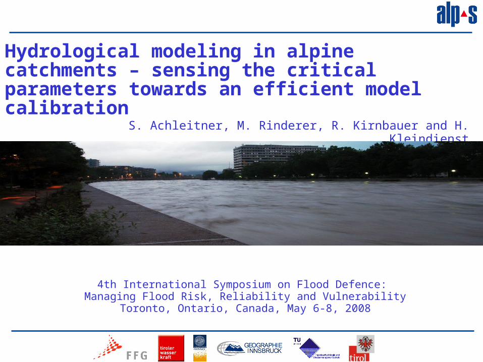
4th International Symposium on Flood Defence: Managing Flood Risk, Reliability and Vulnerability
Toronto, Ontario, Canada, May 6-8, 2008
Hydrological modeling in alpine catchments – sensing the critical parameters towards an efficient model calibration
S. Achleitner, M. Rinderer, R. Kirnbauer and H. Kleindienst
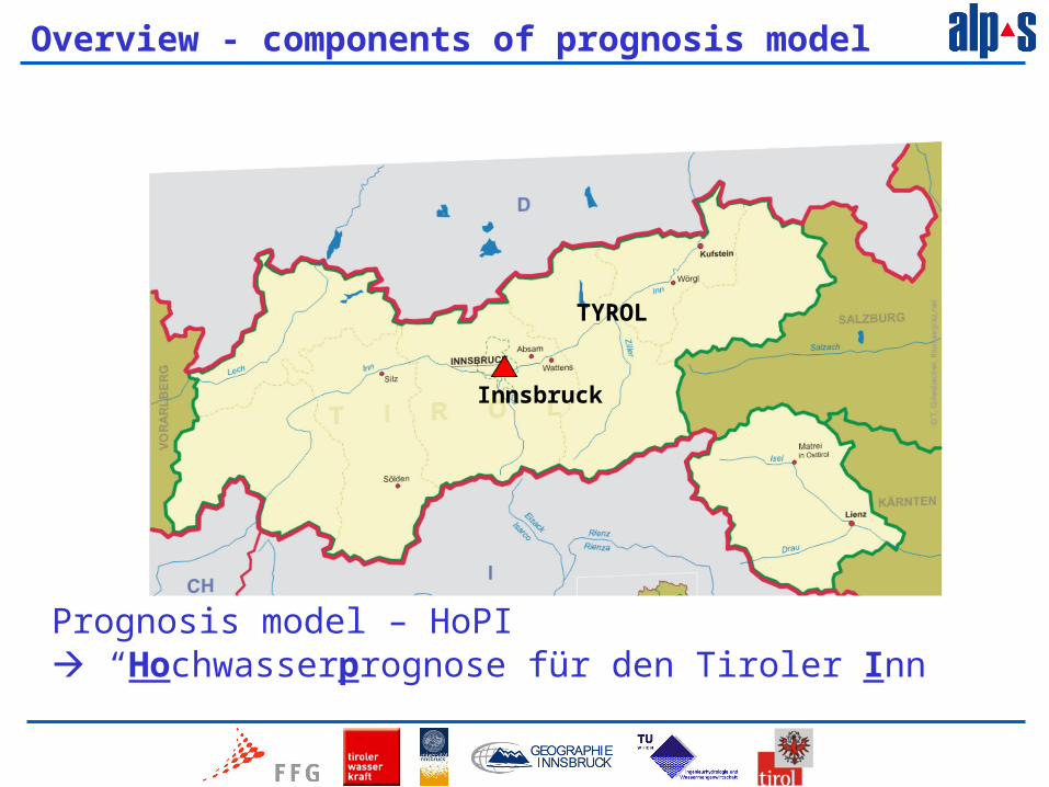
Overview - components of prognosis model
Innsbruck
TYROL
Prognosis model – HoPI “Hochwasserprognose für den Tiroler Inn

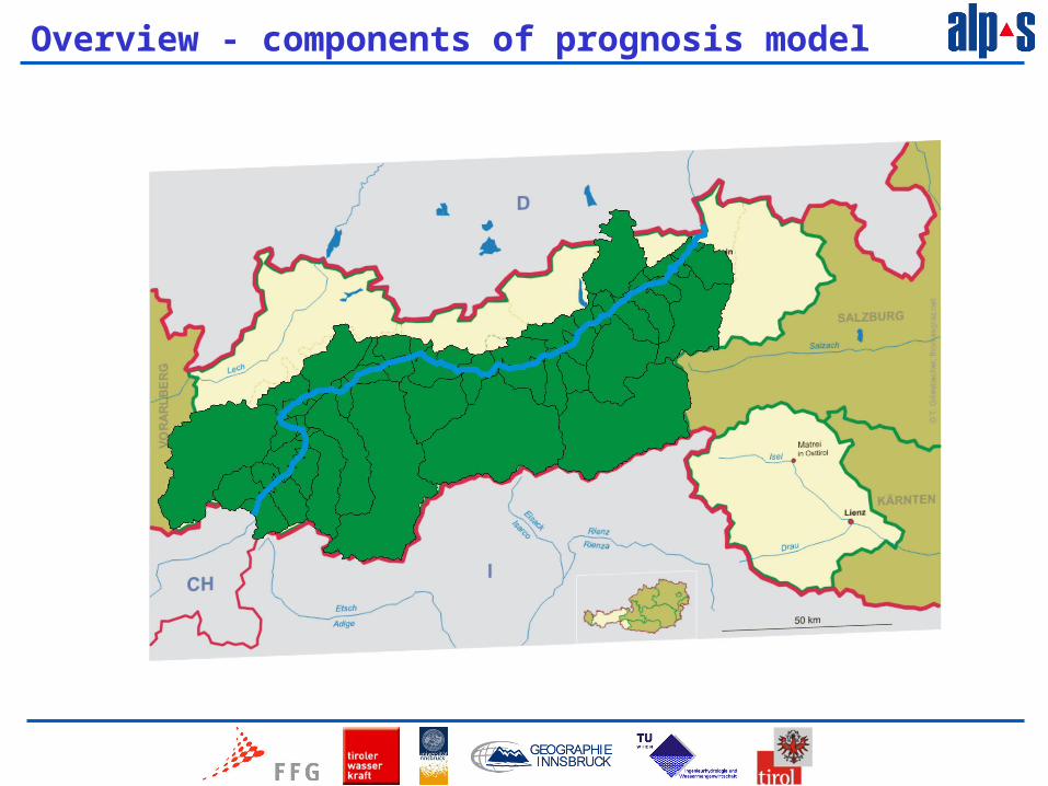
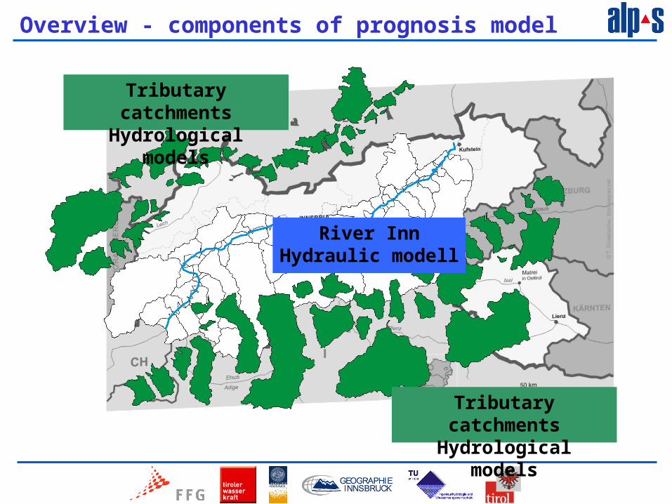
Overview - components of prognosis model
River Inn : 200km from Switzerland to Germany/Bavaria ~ 60 % of the state area (6700 km2) drain into the River Inn
Innsbruck
Prognosis model – HoPI “Hochwasserprognose für den Tiroler Inn

Overview - components of prognosis model
Innsbruck
Largest flood event August 2005 Innsbruck: 1510 m3/s (HQ100= 1370 m3/s)
River Inn : 200km from Switzerland to Germany/Bavaria ~ 60 % of the state area (6700 km2) drain into the River Inn
Overview - components of prognosis model
Overview - components of prognosis model
River InnHydraulic modell
Tributary catchmentsHydrological models
Tributary catchmentsHydrological models
Overview - components of prognosis model
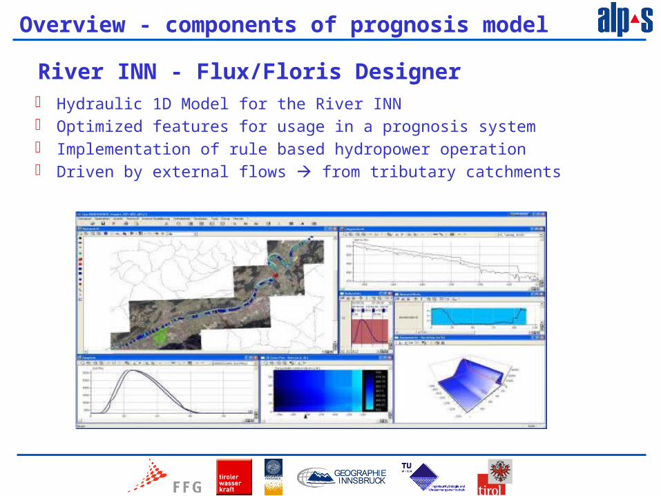
Hydraulic 1D Model for the River INN Optimized features for usage in a prognosis system Implementation of rule based hydropower operation Driven by external flows from tributary catchments
River INN - Flux/Floris Designer
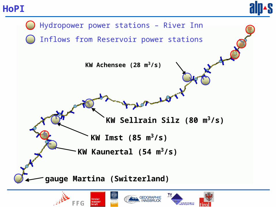
HoPI
Hydropower power stations – River Inn
gauge Martina (Switzerland)
KW Kaunertal (54 m3/s)
KW Imst (85 m3/s)
KW Sellrain Silz (80 m3/s)
KW Achensee (28 m3/s)
Inflows from Reservoir power stations
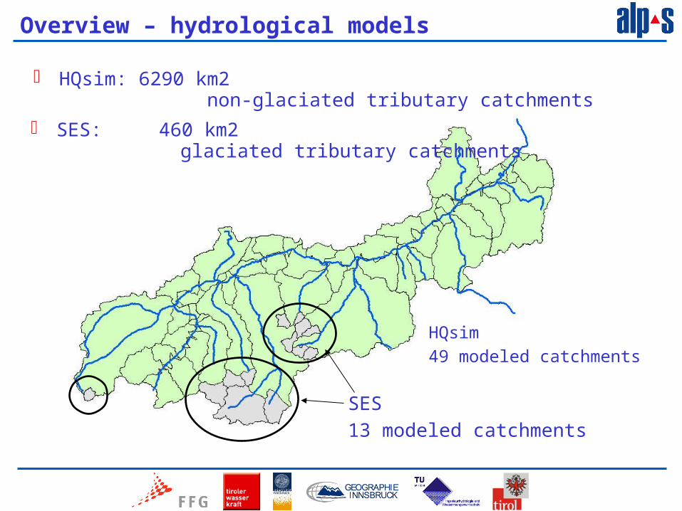
Overview – hydrological models
HQsim: 6290 km2 non-glaciated tributary catchments
SES
13 modeled catchments
HQsim
49 modeled catchments
SES: 460 km2 glaciated tributary catchments

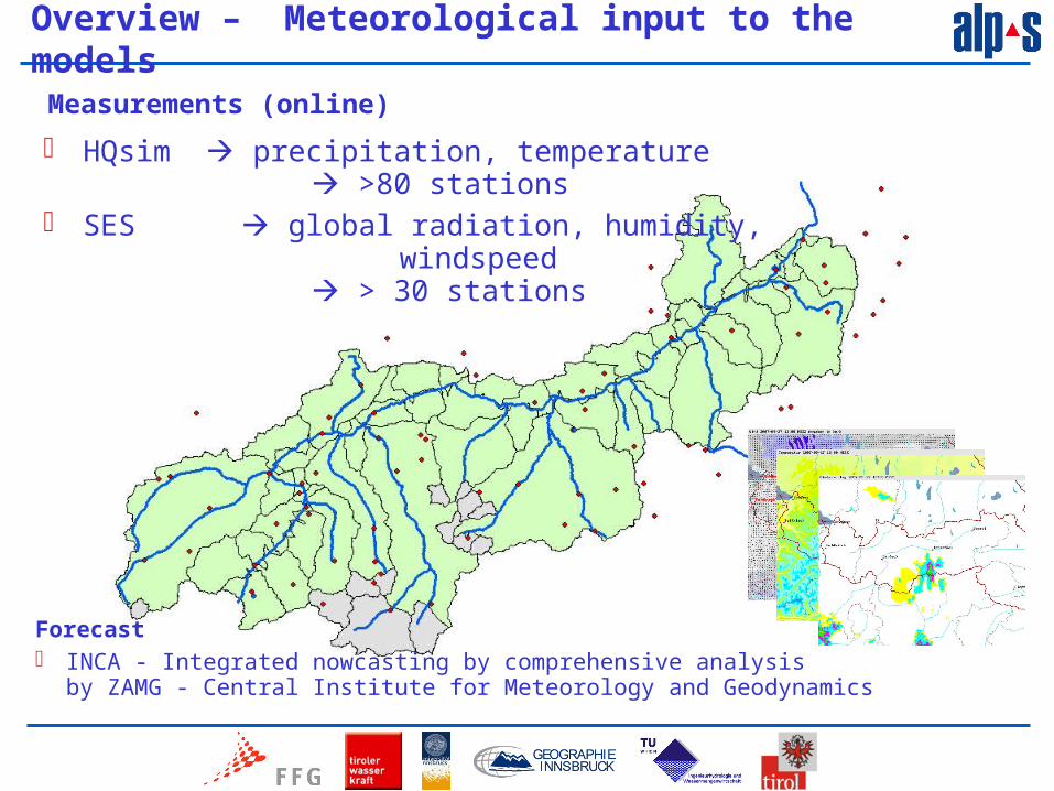
Overview – Meteorological input to the models
Overview – Meteorological input to the models
Forecast INCA - Integrated nowcasting by comprehensive analysis
by ZAMG - Central Institute for Meteorology and Geodynamics
HQsim precipitation, temperature >80 stations
SES global radiation, humidity, windspeed > 30 stations
Measurements (online)
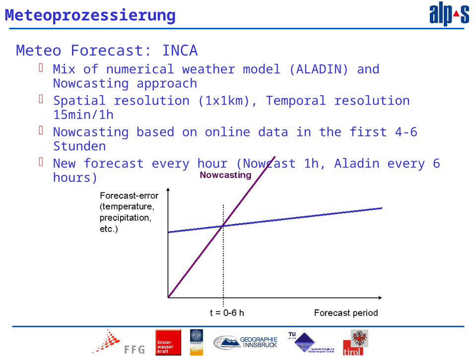
Meteoprozessierung
Meteo Forecast: INCA Mix of numerical weather model (ALADIN) and Nowcasting
approach Spatial resolution (1x1km), Temporal resolution 15min/1h Nowcasting based on online data in the first 4-6 Stunden New forecast every hour (Nowcast 1h, Aladin every 6 hours)

INCA
Online measurement Meteo forecast
Data management - Input, Output, Archive
File based System
SES HQsim FLUX
WEB-Interface
Visualization
Model runsData processing
Spatial and temporal processing of meteo-data, real time control of software components
1x/d1x/h
HoPI - Data and Information flow
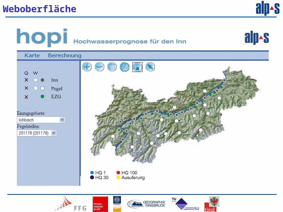
Weboberfläche
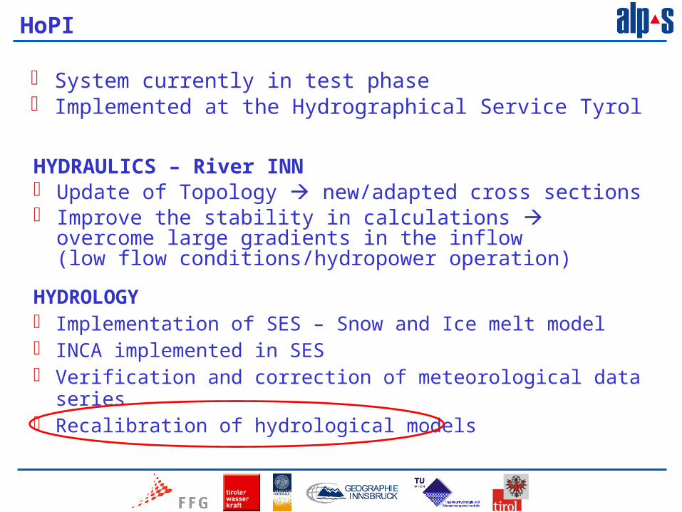
HYDRAULICS – River INN Update of Topology new/adapted cross sections Improve the stability in calculations overcome large
gradients in the inflow(low flow conditions/hydropower operation)
HYDROLOGY Implementation of SES – Snow and Ice melt model INCA implemented in SES Verification and correction of meteorological data series Recalibration of hydrological models
HoPI
System currently in test phase Implemented at the Hydrographical Service Tyrol

Overview - components of prognosis model
Brandenberger Ache
Area: 280 km²Elevation: 500- 2250 m.a.s.l.
HQsim model background
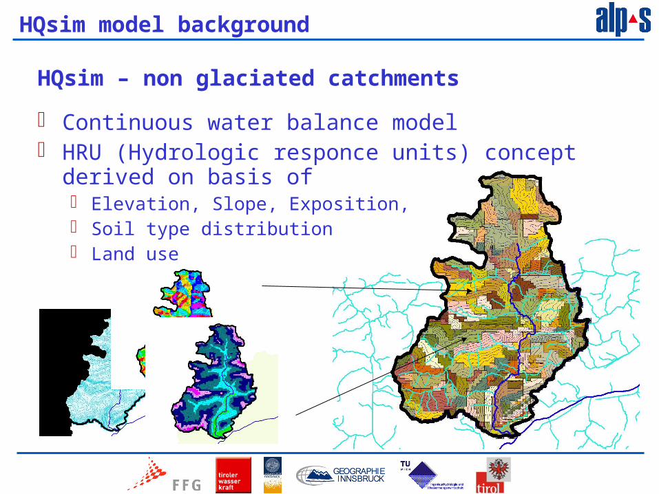
HQsim – non glaciated catchments
Continuous water balance model HRU (Hydrologic responce units) concept
derived on basis of Elevation, Slope, Exposition, Soil type distribution Land use
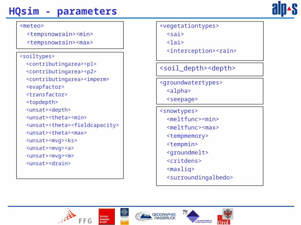
HQsim - parameters<meteo>
<tempsnowrain><min>
<tempsnowrain><max>
<soiltypes>
<contributingarea><p1>
<contributingarea><p2>
<contributingarea><imperm>
<evapfactor>
<transfactor>
<topdepth>
<unsat><depth>
<unsat><theta><min>
<unsat><theta><fieldcapacity>
<unsat><theta><max>
<unsat><mvg><ks>
<unsat><mvg><a>
<unsat><mvg><m>
<unsat><drain>
<vegetationtypes>
<sai>
<lai>
<interception><rain>
<groundwatertypes>
<alpha>
<seepage>
<snowtypes>
<meltfunc><min>
<meltfunc><max>
<tempmemory>
<tempmin>
<groundmelt>
<critdens>
<maxliq>
<surroundingalbedo>
<soil_depth><depth>

HQsim - parameters<meteo>
<tempsnowrain><min>
<tempsnowrain><max>
<soiltypes>
<contributingarea><p1>
<contributingarea><p2>
<contributingarea><imperm>
<evapfactor>
<transfactor>
<topdepth>
<unsat><depth>
<unsat><theta><min>
<unsat><theta><fieldcapacity>
<unsat><theta><max>
<unsat><mvg><ks>
<unsat><mvg><a>
<unsat><mvg><m>
<unsat><drain>
<vegetationtypes>
<sai>
<lai>
<interception><rain>
<groundwatertypes>
<alpha>
<seepage>
<snowtypes>
<meltfunc><min>
<meltfunc><max>
<tempmemory>
<tempmin>
<groundmelt>
<critdens>
<maxliq>
<surroundingalbedo>
<soil_depth><depth><soiltypes>
<contributingarea><p1>
<contributingarea><p2>
<contributingarea><imperm>
<evapfactor>
<transfactor>
<topdepth>
<unsat><depth>
<unsat><theta><min>
<unsat><theta><fieldcapacity>
<unsat><theta><max>
<unsat><mvg><ks>
<unsat><mvg><a>
<unsat><mvg><m>
<unsat><drain>
<soiltypes>
<contributingarea><p1>
<contributingarea><p2>
<contributingarea><imperm>
<evapfactor>
<transfactor>
<topdepth>
<unsat><depth>
<unsat><theta><min>
<unsat><theta><fieldcapacity>
<unsat><theta><max>
<unsat><mvg><ks>
<unsat><mvg><a>
<unsat><mvg><m>
<unsat><drain>
<soiltypes>
<contributingarea><p1>
<contributingarea><p2>
<contributingarea><imperm>
<evapfactor>
<transfactor>
<topdepth>
<unsat><depth>
<unsat><theta><min>
<unsat><theta><fieldcapacity>
<unsat><theta><max>
<unsat><mvg><ks>
<unsat><mvg><a>
<unsat><mvg><m>
<unsat><drain>
<soiltypes>
<contributingarea><p1>
<contributingarea><p2>
<contributingarea><imperm>
<evapfactor>
<transfactor>
<topdepth>
<unsat><depth>
<unsat><theta><min>
<unsat><theta><fieldcapacity>
<unsat><theta><max>
<unsat><mvg><ks>
<unsat><mvg><a>
<unsat><mvg><m>
<unsat><drain>
<soiltypes>
<contributingarea><p1>
<contributingarea><p2>
<contributingarea><imperm>
<evapfactor>
<transfactor>
<topdepth>
<unsat><depth>
<unsat><theta><min>
<unsat><theta><fieldcapacity>
<unsat><theta><max>
<unsat><mvg><ks>
<unsat><mvg><a>
<unsat><mvg><m>
<unsat><drain>
<soiltypes>
<contributingarea><p1>
<contributingarea><p2>
<contributingarea><imperm>
<evapfactor>
<transfactor>
<topdepth>
<unsat><depth>
<unsat><theta><min>
<unsat><theta><fieldcapacity>
<unsat><theta><max>
<unsat><mvg><ks>
<unsat><mvg><a>
<unsat><mvg><m>
<unsat><drain>
<groundwatertypes>
<alpha>
<seepage>
<groundwatertypes>
<alpha>
<seepage>
<groundwatertypes>
<alpha>
<seepage>
<groundwatertypes>
<alpha>
<seepage>
<groundwatertypes>
<alpha>
<seepage>
<groundwatertypes>
<alpha>
<seepage>
<soil_depth><depth><soil_depth><depth>
<soil_depth><depth>
<vegetationtypes>
<sai>
<lai>
<interception><rain>
<vegetationtypes>
<sai>
<lai>
<interception><rain>
<vegetationtypes>
<sai>
<lai>
<interception><rain>
<vegetationtypes>
<sai>
<lai>
<interception><rain>
<vegetationtypes>
<sai>
<lai>
<interception><rain>
<vegetationtypes>
<sai>
<lai>
<interception><rain>
<soiltypes>
<contributingarea><p1>
<contributingarea><p2>
<contributingarea><imperm>
<evapfactor>
<transfactor>
<topdepth>
<unsat><depth>
<unsat><theta><min>
<unsat><theta><fieldcapacity>
<unsat><theta><max>
<unsat><mvg><ks>
<unsat><mvg><a>
<unsat><mvg><m>
<unsat><drain>
HQsim - parameters
Why reducing the parameters?
Too many parameter describing the rainfall-runoff relation
Confusing when calibrating
Auto calibration: less parameters to be considered in a first approach
HQsim model background
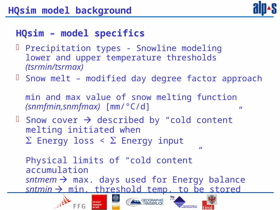
HQsim – model specifics
Precipitation types - Snowline modelinglower and upper temperature thresholds (tsrmin/tsrmax)
Snow melt – modified day degree factor approach min and max value of snow melting function (snmfmin,snmfmax) [mm/°C/d]
Snow cover described by “cold content” melting initiated when Energy loss < Energy input
Physical limits of “cold content” accumulationsntmem max. days used for Energy balancesntmin min. threshold temp. to be stored

HQsim model background
HQsim – model specifics
Contributing area for surface runoff described as arctan function f (saturation)
(s) saturation (i) fraction of seald surface (cap1, cap2) describe the shape of the arctan function
i
capcap
capscapcapcapiCA
cap
cap
1arctan)15.0(arctan
1arctan1)15.0(1arctan1
2
2

HQsim model background
HQsim – model specifics
Water movement in soil(sd) …soil depth (mvgks) …saturated hydraulic conductivity
Unsaturated hydraulic conductivity (k) Mualem van-Genuchten
(mvkm, mvga) Mualem van-Genuchten parameters
2111mvgmmvgmmvga ssmvgksk
Calibration of hydrological models
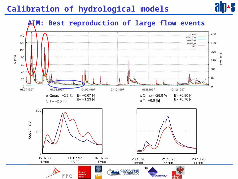
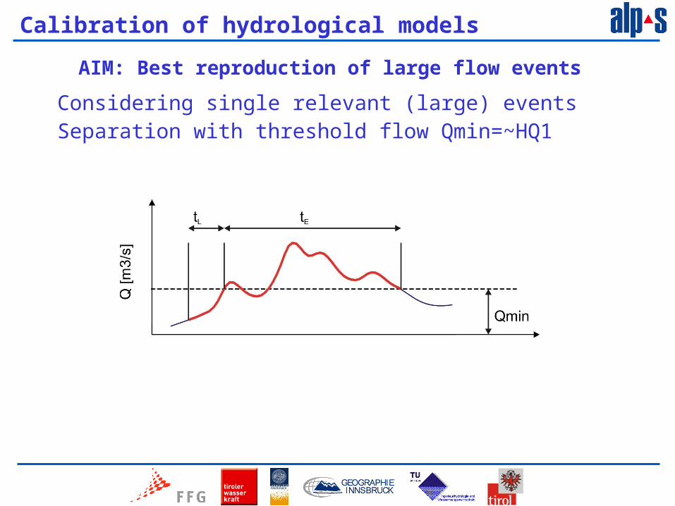
AIM: Best reproduction of large flow events
Calibration of hydrological models
AIM: Best reproduction of large flow events
Considering single relevant (large) eventsSeparation with threshold flow Qmin=~HQ1
Parameter variation
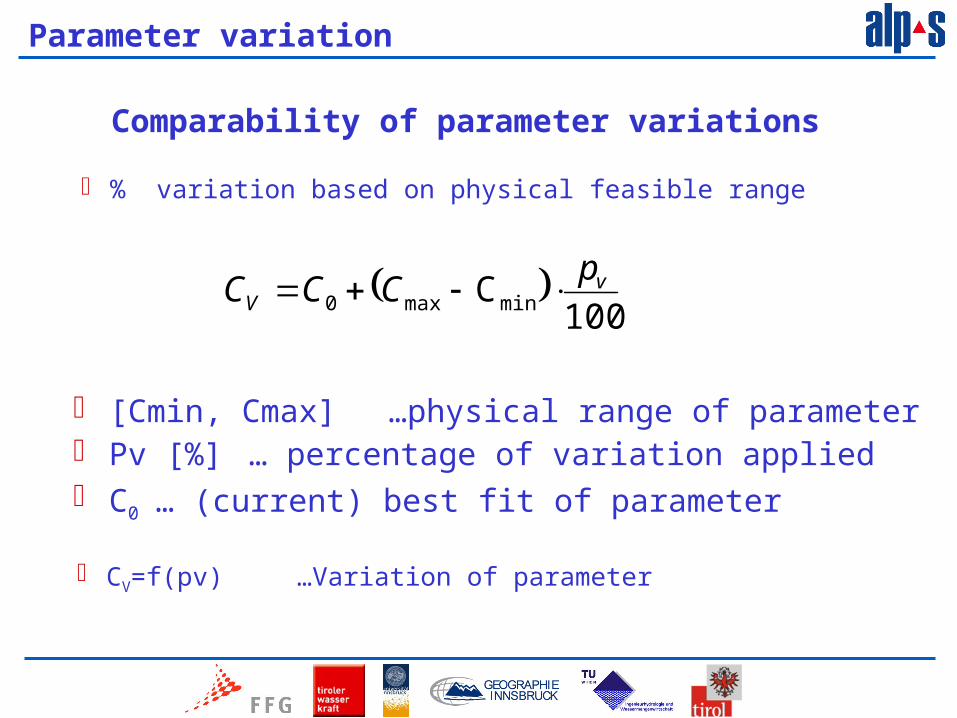
Comparability of parameter variations
% variation based on physical feasible range
100
Cminmax0v
V
pCCC
[Cmin, Cmax] …physical range of parameter Pv [%] … percentage of variation applied C0 … (current) best fit of parameter
CV=f(pv) …Variation of parameter
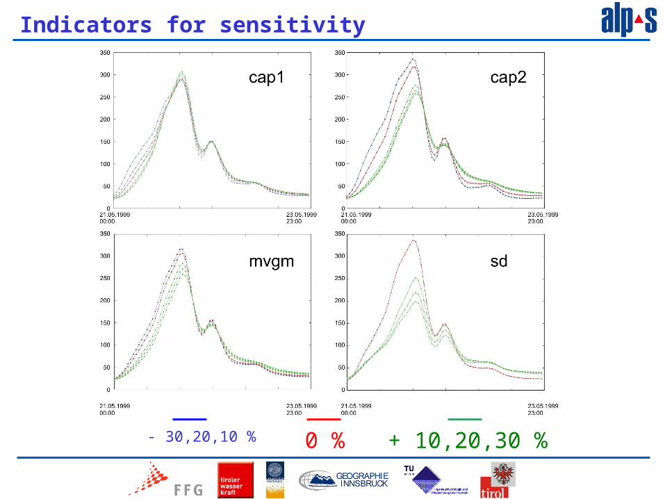
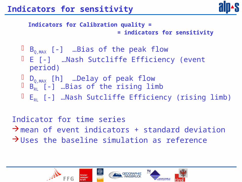
Indicators for sensitivity
- 30,20,10 % 0 % + 10,20,30 %
Indicators for sensitivity
BQ,MAX [-] …Bias of the peak flow E [-] …Nash Sutcliffe Efficiency (event period) DQ,MAX [h] …Delay of peak flow
BRL [-] …Bias of the rising limb ERL [-] …Nash Sutcliffe Efficiency (rising limb)
Indicator for time series mean of event indicators + standard deviationUses the baseline simulation as reference
Indicators for Calibration quality = = indicators for sensitivity

Results
BQ,MAX [-] …Bias of the peak flow
1994
- 2
001
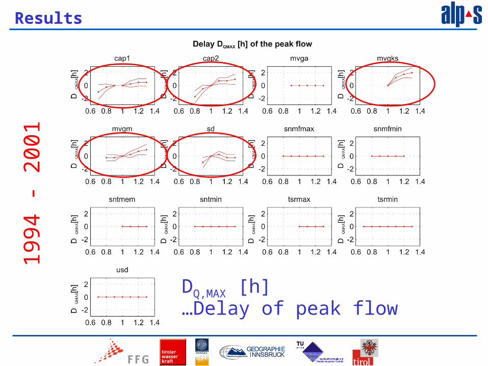
Results
DQ,MAX [h]…Delay of peak flow
1994
- 2
001

Results
E [-]…Nash Suttcliffe Efficiency (event period)
1994
- 2
001
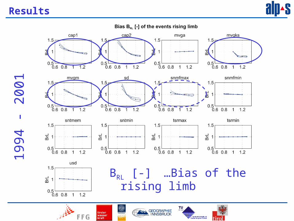
Results
BRL [-] …Bias of the rising limb
1994
- 2
001
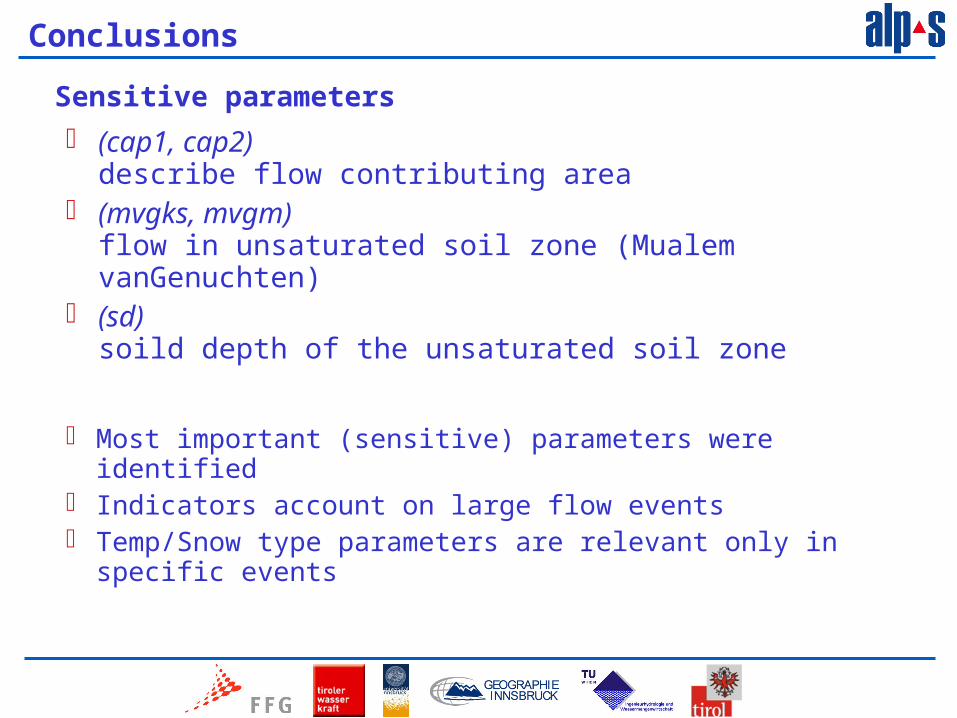
Conclusions
Most important (sensitive) parameters were identified Indicators account on large flow events Temp/Snow type parameters are relevant only in specific
events
(cap1, cap2) describe flow contributing area
(mvgks, mvgm) flow in unsaturated soil zone (Mualem vanGenuchten)
(sd)soild depth of the unsaturated soil zone
Sensitive parameters

HQsim model background
HQsim – non glaciated catchments
Derivation of flow paths/river representations Modeled with linear flow routing
Combination of River paths HRU Flowtimes from HRU 2 flowpaths