4O

MULTIDISCIPLINARY ANDMULTIOBJECTIVE OPTIMIZATION

IN CONCEPTUAL DESIGN FOR MYMIXED-STREAM TURBOFAN ENGINES

THESIS

Luc J.J.P. Nadon, Captain, CAF

AFITIGAE/ENYI96D-6 <7

DEPARTMENT OF THE AIR FORCEAIR UNIVERSIY

AIR FORCE INSTITUTE OF TECHNOLOGY

DIMC QUJALIT lgp'Wright-Patterson Air Force Base, 0hi U1 ION STA ffIN1 A

Approve for public release;

AFIT/GAE/ENY/96D-6

MULTIDISCIPLINARY ANDMULTIOBJECTIVE OPTIMIZATION

IN CONCEPTUAL DESIGN FORMIXED-STREAM TURBOFAN ENGINES

THESIS

Luc J.J.P. Nadon, Captain, CAF

AFIT/GAE/ENY/96D-6

Approved for public release; distribution unlimited

DTIC QUALrY fT ID

Disclaimer Statement

The views expressed in this thesis are those of the author and do not reflect the officialpolicy or position of the Department of Defense, the U.S. Government, the CanadianDepartment of National Defense, or the Canadian Government.

AFIT/GAE/ENY/96D-6

MULTIDISCIPLINARY ANDMULTIOBJECTIVE OPTIMIZATION

IN CONCEPTUAL DESIGN FOR MIXED-STREAM TURBOFAN ENGINES

THESIS

Presented to the Faculty of the School of Engineering of the

Air Force Institute of Technology

Air University

In partial Fulfillment of the Requirements for the Degree of

Master of Science in Aeronautical Engineering

Luc Nadon, B.S.M.E.

Captain, CAF

December 1996

Approved for public release; distribution unlimited

Acknowledgment

This thesis would not have been possible without the outstanding support from a

number of people whom I would like to take this opportunity to thank. First, I need to

express my most sincere gratitude to LCol S. Kramer for directing me into research on

optimization. Moreover, I wish to let him know how I appreciated his common sense

approach to problems and his heartfelt moral support in dire straits. I am indebted to the

committee members, Dr. P. I. King and Maj. E. Pohl, for the priceless advice they

provided in their respective field. I would like to thank Mr. J. M. Stricker at Wright

Laboratories for his help with the problem definition and his enthusiastic support for the

project. I would also like to express my gratitude to Mr. R. E. Fredette, from Universal

Technology Corporation, for the comprehensive Global Strike Aircraft data he provided.

I need to recognize the invaluable support given by Dr. J. D. Mattingly, From Seattle

University, for providing the ONX, OFFX and MISS computer original Fortran computer

codes, without which the Matlab engine analysis codes could not have been created. Last,

but not least, I want to thank K. Larsen, the engineering computer lab system manager, for

her precious guidance in dealing with the many computer-related hurdles I encountered

throughout this project.

Luc J.J.P. Nadon

ii

Table of Contents

Page

Acknowledgments .................................................. nH

List of Figures .................................................... vi

List of Tables .................................................... vii

List of Symbols.................................................... ix

Abstract......................................................... xiv

1. Introduction ..................................................... 1I

Background ..................................................... 1IProblem Statement ................................................ 3Scope.......................................................... 3Thesis Overview.................................................. 4

II. Analysis Fundamentals ............................................. 6

Introduction..................................................... 6General Optimization Concepts....................................... 6Multidisciplinary (MDO) and Multiobjective (MOO) Optimization ............... 9Sequential Quadratic Programming.................................... 13Matlab 'constr' SQP Optimization Code................................ 16Theory of Genetic Algorithms....................................... 16

General Concept ............................................. 16Constraints and Penalty Functions................................. 18

GAOT GA Matlab Computer Code................................... 20On-Design Cycle Analysis.......................................... 20Off-Design Cycle Analysis.......................................... 26Mission Analysis................................................. 31Takeoff Gross Weight (WTo) Determination .............................. 35Aircraft Cost Model .............................................. 39

Engine Annulus Area M odel ........................................... 41M iscellaneous constraint equations ...................................... 44

Compressor Exit Pressure ......................................... 44Compressor Exit Temperature ..................................... 45Low Pressure Spool Rpm ......................................... 45High Pressure Spool Rpm ......................................... 45High Pressure Turbine Specific Work ................................ 45

Global Strike Aircraft and Short Range Interceptor ......................... 46Global Strike Aircraft (GSA) ...................................... 47Short Range Interceptor (SRI) ..................................... 49

III. M ethodology ..................................................... 54

Introduction ....................................................... 54O bjectives ........................................................ 54A ssum ptions ....................................................... 55Optimization Problems Statements ...................................... 56Cases Investigated .................................................. 60Overall Taken to Achieve Thesis Objectives ............................... 62

Matlab as a Programming Environment ............................... 63Creation of the On-Design Analysis Computer Code ........................ 64Creation of the Off-Design Analysis Computer Code ........................ 66Creation of the Mission Analysis Computer Code ........................... 69On-Design Optimization Process .............................. t ......... 72

On-Design Objective Function ..................................... 77Optimization with M ission Process ...................................... 79

W TO Convergence ............................................... 83Mission Optimization Objective Function ............................. 88

IV . Findings and Analysis ............................................... 92

Introduction ....................................................... 92General Comments and Observations .................................... 92Case 1: Test Case with Short Range Interceptor ............................ 98Case 2: Short Range Interceptor On-design Mono-Objective Optimization ....... 101Case 3: Short Range Interceptor Mono-Objective Mission Optimization ......... 103

Modified SRI Full Mission Optimization ............................. 109Case 4: Global Strike Aircraft Mono-Objective Mission Optimization ........... 110Case 5: Global Strike Aircraft Multiobjective Mission Optimization ............ 114Case 6: Global Strike Aircraft Multiobjective On-Design Optimization .......... 118

iv

V. Conclusions and Recommendations.................................. 121

Introduction ................................................... 121Conclusions ................................................... 121Recommendations............................................... 125

Appendix A: Instructions on How to Obtain Optimization and Engine AnalysisComputers Codes........................................ 126

Appendix B: Drag Profiles........................................... 127

Appendix C: Engine Optimization Computer Codes Operating Instructions ........ 129

Bibliography..................................................... 154

Vita............................................................ 156

v

List of Figures

Figure Page

1. Optimum D esign Process .............................................. 7

2. Two-Discipline M DO Process ......................................... 10

3. Engine Reference Stations - Mixed Flow Turbofan .......................... 23

4. Off-Design Solution Scheme - Part One .................................. 29

5. Off-Design Solution Scheme - Part Two .................................. 30

6. Mission Analysis Flow Chart for a Leg ................................... 35

7. On-Design Optimization Process (gaondes.m) ............................. 76

8. On-design Global Optimization Objective Function Process (gafunbis.m) ......... 78

9. On-Design Local Optimization Objective Function Process (fun.m) ............. 79

10. Engine Optimization with Mission Process (gaoptmiss.m) - Part One ........... 82

11. Engine Optimization with Mission Process (gaoptmiss.m) - Part Two ........... 83

12. Global Mission Optimization Objective Function Process (gafunmiss.m) ......... 89

13. Local Mission Optimization Objective Function Process (funmiss2.m) .......... 90

14. CDO vs. Flight Mach Number, M0, for the Short Range Interceptor ............ 127

15. K1 vs. Flight Mach Number M0, for the Short Range Interceptor ............. 127

16. CD0 vs. Flight Mach Number, M0 for the Global Strike Aircraft ............... 128

17. K, vs. Flight Mach Number, M0, for the Global Strike Aircraft ............... 128

vi

List of Tables

Table Page

1. On-Design Analysis Inputs, Outputs and Parameters ......................... 22

2. Off-Design Analysis Inputs, Outputs and Parameters ........................ 31

3. M ission Analysis Legs ............................................... 34

4. Global Strike Aircraft Mission Profile .................................... 48

5. Global Strike Aircraft Optimization Data ................................. 49

6. Short Range Interceptor Mission Profile .................................. 51

7. Short Range Interceptor Optimization Data ............................... 52

8. Trial-and-Error Process Short Range Interceptor Optimum Design .............. 53

9. Variables and Linear Scaling Boundaries for Case 1: SRI Test Case ............ 99

10. Final Results for Case 1: SRI Test Case ................................ 100

11. Variables and Linear Scaling Boundaries for Case 2:SRI On-Design Optimization ........................................ 102

12. Final Results for Case 2: SRI On-Design Optimization ..................... 103

13. Variables and Linear Scaling Boundaries for Case 3:SRI M ission Optimization .......................................... 105

14. Final Results for the Case 3: SRI Mission Optimization .................... 106

15. SRI Design Variables Values at M = 1.6 and h = 35,000 ft .................. 108

16. Variables and Linear Scaling Boundaries for Case 4:GSA Mono-Objective Mission Optimization ............................. 111

17. Final Results for Case 4: GSA Mono-Objective Mission Optimization ......... 112

18. Variables and Linear Scaling Boundaries for Case 5:GSA Multiobjective Mission Optimization .............................. 115

vii

19. Final Results for Case 5: GSA Multiobjective Mission Optimization ........... 115

20. Variables and Linear Scaling Boundaries for Case 6:GSA On-Design Optimization ....................................... 119

21. Final Results for Case 6: GSA On-design Optimization ..................... 120

viii

List of Symbols

A - Area (ft2)A* - Area corresponding to M = 1 (ft2)a - Speed of sound, coefficient in F function equation (ft/s)b - coefficient in F function equationC1 - Engine cost coefficient ($/lb thrust)C2 - Avionics cost coefficient ($)C3 - Airframe cost coefficient ($/lb empty weight)CD - Drag coefficientCL - Lift coefficientCp - Specific heat at constant pressure (BTU/lbm-R)C., - Specific heat at constant volume (BTU/Ibm-R)CTO - Power takeoff shaft coefficientD - Diameter (ft)d - Search directione,. - Polytropic efficiency of faneH - Polytropic efficiency of high pressure compressoret - Polytropic efficiency of turbineetH - Polytropic efficiency of high pressure turbineeti, - Polytropic efficiency of low pressure turbineF - Uninstalled thrust, global objective functionf - Fuel-to-air ratio of burner, objective functionfAB - Fuel-to-air ratio of afterburnerfo - Overall engine fuel-to-air ratioG - Constraint penalty functiong - Acceleration (ft/s2) inequality constraintH - Hessianh - Altitude (ft), equality constraint, enthalpyhpR - Heating value of fuel (BTU/lbm)K - Objective weight factorKI - Coefficient in lift-drag polar equationK2 - Coefficient in lift-drag polar equationkTo - Velocity ratio at takeoffL - Lagrangian functionM - Mach number, Material modifierMFP - Mass flow parameterm - Mass flow rate (Ibm/s)nci - Corrected mass flow at station I (Ibm/s)

N - Rotational speed (rpm), number of 360' turnsNeng - Number of enginesn - Load factorP - Pressure (psi), power (W)

ix

P. - Weight specific excess power (W/lb)PTO - Power of takeoff shaft (W)Pt - Total pressure (psi)q - Dynamic pressure (lb/ft2)R - Gas constant (BTU/Ibm-R), parasitic drag (lb)r - Radius (ft), penalty parameterrmc - remaining fuel coefficientS - Uninstalled thrust specific fuel consumption (1/hr), wing area (ft2)

sf - Scaled objective functionT - Temperature (R), installed thrust (lb)t - Time (s)TSFC - Installed thrust specific fuel consumption (1/hr)Tt Total temperature (R)U - Discipline codeu - Axial velocity (ft/s)W - Weight (lb)WE - Empty weight (lb)Weng - Engine weight (lb)WF - Fuel weight (lb)Wi Weight at beginning of mission leg (lb)Wp Payload weight (lb)WpE - Expended payload weight (lb)Wp - Permanent payload weight (lb)Ws Aircraft structural weight (lb)WTo - Takeoff weight (lb)x - design variableze - Energy height (ft)

c - Bypass ratio, thrust lapse, step length parameter0 - Fuel fraction, bleed air fractionA - Change5 - Static pressure ratio (P/PsL)

61 - Cooling air #1 mass flow rate fraction&2 - Cooling air #2 mass flow rate fraction

- Loss coefficient, global objective function with penaltiesF - Empty aircraft weight fractionY - Ratio of specific heatT1 - EfficiencyTlAB - Efficiency of afterburnerTib - Efficiency of burnerTIC, - Efficiency of fan1lcH - Efficiency of high pressure compressorlid - Diffuser adiabatic efficiency

x

TIM - Power transfer efficiency of shaftlrHa- - Power transfer efficiency of high pressure spool

7l - Power transfer efficiency of low pressure spool,n,, - Power transfer efficiency of power takeoff shaft

rIR - Inlet total pressure recovery11tH - Efficiency of high pressure turbine11tL - Efficiency of low pressure turbineX - Lagrange multiplier[1 - Total pressure ratio, weight fractionrIAB - Total pressure ratio of afterburnerrib - Total pressure ratio of burnerfic - Total pressure ratio of compressorILH - Total pressure ratio of high pressure compressorIL, - Total pressure ratio of fan[1 - Total pressure ratio of diffuser (inlet)Ildm x - Total pressure loss in diffuser (inlet) due to frictionIIm - Total pressure ratio of mixerII ,, - Total pressure loss in mixer due to frictionII. - Total pressure ratio of nozzle

Hr - Isentropic freestream recovery pressure ratioIItH - Total pressure ratio of high pressure turbineIItL - Total pressure ratio of low pressure turbine0 - Static temperature ratio (T/TsL)p - Density (lbm/ft3 )C - Static density ratio (P/PSL)"t - Total temperature ratioTb - Total temperature ratio of burnerr, - Total temperature ratio of compressortcH - Total temperature ratio of high pressure compressor'cc, - Total temperature ratio of fanTd - Total temperature ratio of diffuser (inlet)"tM - Total temperature ratio of mixerTm - Total temperature ratio of station 4 to 4at.2 - Total temperature ratio of station 4c to 4b"t. - Total temperature ratio of nozzleTr - Adiabatic freestream recovery temperature ratio"tH - Total temperature ratio of high pressure turbine"ttL - Total temperature ratio of low pressure turbineX - Enthalpy ratio of burner

- Normalized high pressure turbine inlet temperature (Tt4/TsL)

xi

Subscripts

AB Afterburnera - Inlet annulusav - Availableb - BurnerC - Core flowc - Compressor, correctedc' -FancH - High pressure compressorcl - Cooling air #1c2 - Cooling air #2D -Dragdry - No afterburninge -ExitF - Bypass flowf - Fuel, finalhub - At engine hubi Inlet, initialM - Mixerml - Coolant mixer 1m2 - Coolant mixer 2max - Maximum, with afterburnermin - MinimummH - Mechanical, high pressure spoolmL - Mechanical, low pressure spoolmP - Mechanical, power takeoff shaftN - iteration variablen - NozzleR - Rotation, Referencereq - Requiredspec - SpecificSTALL - Corresponding to stallTO - Takeoff, power takeoffTR - Transitiont - Turbine, totaltip - At tip of bladesTH - Overall efficiencytH - High pressure turbine

xii

tL - Low pressure turbinewet - With afterburningO- 10 - Engine station location

%, - isentropic freestream recovery

Superscripts

0* - Corresponding to M = 1

xiii

AFIT/GAE/ENY/96D-6

Abstract

Despite major advances in design tools such as engine cycle analysis software and

computer-aided design, conceptual gas turbine engine design is essentially a trial-and-error

process based on the experience of engineers. Modern optimization concepts, such as

multidisciplinary optimization (MDO), and multiobjective optimization (MOO), linked

with sequential quadratic programming (SQP) methods and genetic algorithms (GA), were

applied to the conceptual engine design process to automate the conceptual design phase.

Robust integrated computer codes were created to find the optimal values of eight engine

parameters in order to minimize fuel usage, aircraft cost and engine annulus area over a

given mission. The engine cycle selected for study was the mixed-stream, low-bypass

turbofan. SQP and GA optimization algorithms were integrated with on-design and off-

design engine cycle analysis and mission analysis computer codes created by the authors to

obtain the optimized conceptual engine design for an imaginary short range interceptor

and the Global Strike Aircraft U.S. Air Force concept. The process used a non-specific

approach that can be applied to a wide variety of missions and aircraft. All the codes were

written in Matlab, and so operate under the same programming architecture and can be

easily upgraded or modified.

xiv

MULTIDISCIPLINARY AND MULTIOBJECTIVE OPTIMIZATIONIN CONCEPTUAL DESIGN FOR MIXED-STREAM TURBOFAN

ENGINES

I. Introduction

Background

The aircraft engine design and manufacturing fields are extremely competitive

since multimillion, if not multibillion, dollar contracts are involved. Small variations in the

selection of engine design parameters may have a significant impact on the thrust available,

the quantity of fuel consumed over a mission, or the costs of the engine and aircraft.

Unfortunately, engine design is an inexact science that involves a trial-and-error process

based on engineers' and corporate experience. This is due do the fact that a gas turbine

engine is a sophisticated device which involves complex interactions of factors such as 3-

D viscous and turbulent flows, material stresses, and thermodynamics, to name a few. The

design process search for a design that meets all thrust requirements at the lowest cost and

fuel consumption. This process is based on empirical models (obtained through

experience and experiments) and hopefully leads to an overall lighter and cheaper aircraft

(15: 12.1-12.3).

This search in a complex environment for the best engine design is well suited for

multidisciplinary optimization (MDO) and multiobjective (MOO) approaches.

Optimization involves the determination of optimal values for a given set of design

1

variables (such as turbine inlet temperature and compressor pressure ratio) to minimize or

maximize a given function (such as fuel consumption). It does so by performing searches

for minima (or maxima) over the design space with the use of numerical algorithms.

MDO involves the application of multiple engineering fields, such as aerodynamics and

materials, in the optimization of complex design problems. In the aerospace world, MDO

has been successfully applied to the structures and controls field. MDO is a relatively new

tool in aircraft engine design and includes such disciplines as thermodynamics,

aerodynamics, material stresses and cost analysis. Multiobjective optimization is

concerned with the integration in the objective function of multiple objectives to minimize

(maximize). These objectives may span one or many disciplines. Most efforts in this

promising field have concentrated on the optimization of only a few engine design

parameters or the optimization was carried out over only a few flight conditions, or for a

specific aircraft. What is needed is an integrated tool that can be used for any number of

variables and over a wide range of engine types and flight conditions.

As the function to be minimized (or maximized) becomes more complex, and as

the number of design variable increases, the location of the optimal design point becomes

increasingly hard to determine and many algorithms simply cannot converge toward an

optimal solution. Among the most powerful calculus-based optimization approach is

sequential quadratic programming (SQP). SQP converge to a local minima (or maxima)

with the use of quasi-Newton and quadratic programming methods. An example of SQP

algorithm is the Matlab 'constr.m' code (6). Another promising (and somewhat recent)

technique used in these situations is the genetic algorithm (GA). Genetic algorithms apply

2

aspects of biological genetic theory, such as reproduction and mutations, to select optimal

design through an evolutionary process. One such algorithm is GAOT, developed at

North Carolina State University (7). Both GA and SQP were integrated into a single

algorithm in the present project to exploit strengths of each technique. These optimization

tools are used in conjunction with mission analysis, on-design and off-design cycle analysis

codes created by the author, based on methods by Mattingly (10), in order to obtain an

optimal conceptual engine. The model thus created is modular and meant to be improved

and updated by considering additional disciplines such as stresses and installation losses.

Problem Statement

The need exists to improve the trial-and-error conceptual engine design process.

A conceptual engine design should meet all mission and flight requirements with the

lowest fuel usage, cost, and engine size. The methodology selected to solve the

aforementioned problem must consider a modular optimization model to allow for the

inclusion of additional factors such as stresses, installation losses, and advanced cost

models. As examples, optimal conceptual designs will be developed for the DOD Global

Strike Aircraft concept (4) and for an imaginary short range interceptor previously

investigated by the author using a trial and error process.

Scope

This project applied a multidisciplinary and multiobjective optimization approach

and used sequential quadratic programming and genetic algorithms in conjunction with

3

engine cycle and mission analysis codes, and simple aircraft cost and engine size models to

develop an engine design process applicable to optimized engine uninstalled performance

over a whole mission, from takeoff to landing. The engine cycle and mission analysis

codes will be called as part of the objective function. The engine cycle under study was

the mixed-stream, low bypass turbofan. It was selected because of its increasing use for

military aircraft applications.

Thesis Overview

The engine design optimization process is developed in the following chapters of

this thesis:

Chapter II. The theory and analytical tools used in the optimization procedure are

covered. Concepts like optimization, genetic algorithms, sequential quadratic

programming methods, on-design and off-design cycle analysis and mission

analysis are briefly discussed. This chapter also includes descriptions of the

computer codes used and the characteristics of the Global Strike Aircraft and

the short range interceptor.

Chapter III. This chapter summarizes the methodology is in solving the optimization

problem. Thesis objectives and assumptions are stated and the optimization

problem is formulated in details. The optimization processes for both the

single flight condition and the full mission cases are described.

4

Chapter IV. The project findings and analysis are covered in this chapter. It describes the

results obtained for both the Global Strike Aircraft and the short range

interceptor. Problems and discrepancies are discussed at this point.

Chapter V. An overview of the optimization process, including its results, is provided.

Conclusions and recommendations are presented. The thrust of future research

based on this project is discussed.

5

I. Analysis Fundamentals

Introduction

This chapter covers the theory and tools used in this thesis. These include

optimization, sequential quadratic programming and genetic algorithms, engine cycle

analysis, and mission analysis. All the engine theory introduced is applied to a mixed-

stream, low-bypass turbofan cycle. Also introduced therein are the Global Strike Aircraft

and the short range interceptor.

General Optimization Concepts

The purpose of optimization is to find the values of design variables to minimize

(or maximize) a given function. Simply put, the process search for the function minima

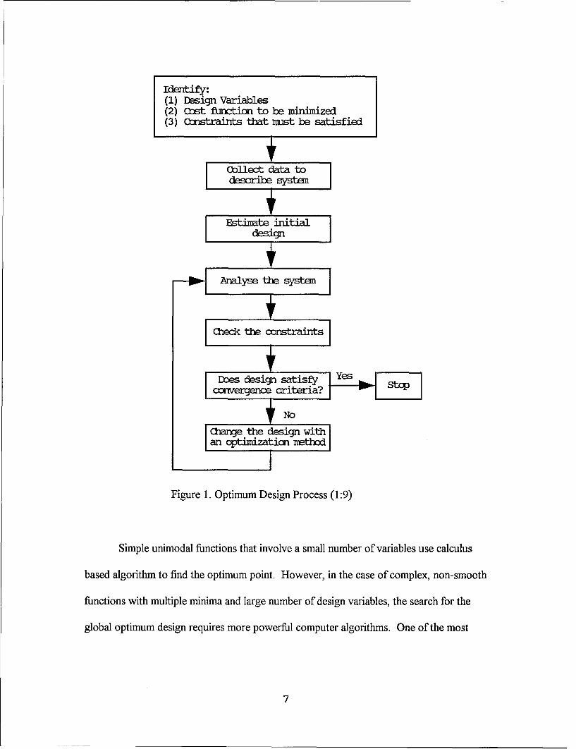
(or maxima). The overall process is described in Figure 1. The terms 'objective function',

'design variables', and 'constraints' need to be defined at this point.

The objective function, also called cost function, is the function to be minimized

(or maximized). Objective functions may be equations or, in the case of complex problem,

outputs from computer codes. The variables that describe the problem and define a given

design are the design variables. Design constraints are the limitations imposed on the

design variables or the objective function to ensure a feasible design is within given

resources and requirements (1:22).

6

Identify:(1) Design Variables(2) ost function to be minimized(3) Qntraiyts that mast be satisfied

Collect data to

Estirate initialdesignI

-- Analyse the s , t

F _ec the osrit

I Ivconvergene criteriaSt

Chanqe the design withan cptimization nethcd

Figure 1. Optimum Design Process (1:9)

Simple unimodal functions that involve a small number of variables use calculus

based algorithm to find the optimum point. However, in the case of complex, non-smooth

functions with multiple minima and large number of design variables, the search for the

global optimum design requires more powerful computer algorithms. One of the most

7

effective calculus-based constrained optimization algorithm is sequential quadratic

programming (SQP). SQP is the method used in this thesis and is described in more

details below. Another extremely powerful tool is the genetic algorithm which is also

discussed below.

The standard optimization problem formulation is as follows (1:45):

minimize f(x) = (x1, x2, x3 , ... , Xn) (1)

Subject to: hi(x) - hj(xi, x2, x3, ... , x.) = 0j = top

gi(x) gi(xI, x2, x3, ... , Xn) !5 0i= tom

where f(x) is the objective function, 'x' is a design variables vector of size n, hj(x)

represent p equality constraints and gi(x) represents m inequality constraints. All

constraints are standardized to the form '= 0' or '_< 0' to simplify optimization algorithms.

A constraint of the form 'a _ gk(x)-- b' is called a side constraint and it defines the

boundaries for a given design variables. Side constraints are expressed in standard form

by breaking them down into two constraints, '-gk(x) + a 0' and 'gk(x) - b < 0'. A

constraint is considered active if the value of the variable or parameters of interest has hit

the constraint limit, i.e. g(x) = 0. Active constraints are a good indicator of the factors

that limits the performance of a given design as they indicate which constraints actively

restrict improvements on a design.

8

Maximization problems are transformed into minimization problems by the

multiplication of the objective function by -1; i.e. the maximization of z(x) is treated as the

minimization of f(x) = -z(x).

Multidisciplinary (MDO) and Multiobjective Optimization (MOO)

The purpose of MDO is to find the optimum values for a set of design variables

dependent on functions from various engineering disciplines. This implies that the output

of one or more disciplines are required as input to one or more other disciplines and vice-

versa. The various disciplines may or may not share the entire set of design variables.

Figure 2 summarizes the MDO process for a two-discipline problem. One can see that the

output for each discipline's code, U1 and U2, feed into the other code and into the

optimizer (3). The optimizer, in turn, evaluates new values for the design variable vector,

XD, that are used as input for both discipline codes. This process is repeated until an

optimum design is reached that satisfies the requirements of both disciplines.

9

Optimizer

XD _U,,U2

Solver, Solver,

Discipline Discipline# 1

# 2

Overall Solver

Figure 2. Two-Discipline MDO process (3:767)

The goal of multiobjective optimization is to determine an optimum design that

involves the minimization (or maximization) of multiple objective functions. More often

than not, these various functions have conflicting objectives, such as the maximization of

performance and the minimization of costs. MOO may or may not involve functions from

different disciplines. A simple approach to MOO is to create a global objective function as

follows:

F(x) = Kisfi(x) + K2sf2(x) + .... + Knsfn(x) (2)

10

where

F(x) = global objective function

Kk = objective weight factors

fk = individual objective functions

sfk = scaled objective function values

n = number of objectives

The value of each individual objective function is scaled in order to ensure that the

value of each term of the global function is of the same order of magnitude. This is

necessary to avoid terms with high magnitude having a disproportionate impact on the

global function. For example, if the value of one objective is expressed in thousands of

thrust pounds of thrust and another objective is expressed in millions of dollars, the cost

term would dominate, even though cost might not be the most critical term of the global

function.

Linear scaling, with individual objective values scaled between zero and one, was

selected for this thesis mainly because of its simplicity. Linear scaling consists in the use

of linear expressions to determines the scaled value of each individual. The linear

expressions are of the form y=ax+b and are based on expected minimum and maximum

values (based on experience) of a given objective, and on how desirable these values are.

The desirable limit is assigned a value of one and the undesirable value is assigned a value

of zero. For example, if a given objective is total aircraft cost and the cost of the aircraft

is expected to vary between $10,000,000 and $30,000,000, the $10,000,000 limit is

11

assigned a value of one while the $30,000,000 is assigned a value of zero since a low cost

is more desirable than a high cost. With the objective limits and their desirability

determined, the scaled value for the given objective is expressed as follows:

Sfk I1 (f, - undesir)(3= (desir - undesir) k (3)

where

desir = value of the given objective desirable limit

undesir = value of the given objective undesirable limit

Equation (3) is a linear expression. The process described above is repeated for

each term of the global objective function. It is important to note that the minimization of

a variable becomes a maximization problem when this variable is linearly scaled since high

scaled values are desirable.

The weight factors Kk are assigned by the designer(s) to vary the impact of each

objective on the global objective function. A relatively high value of K means that the

objective has a higher impact or priority and vice-versa. Kk values are assigned by

experience and must take into account the ultimate goal of a design (i.e. for example, is it

more important to have high performance or a low cost?). Integer Kk values were used in

this thesis. For example, if the first objective of a global function is assigned K1=2 and the

second objective is assigned K2=1, then the first objective has twice the impact of the

12

second one. The default is Kk=l for all three objectives (fuel usage, cost, and area),

which mean that each objective has an equal impact on the global objective function.

Sequential Quadratic Programming

SQP is an advanced nonlinear programming method. The technique attempts to

mimic Newton approaches by using quasi-Newton methods to approximate thejHessian of

the Lagrangian at each iteration of the optimization process. These approximations are

used to generate a quadratic subproblem (QP) which, in turn, is used to determine the

search direction for a line search (6). The Lagrangian function is expressed as follows:

L(R, X) = f(k)+ Xigi(K) (4)i=l

where

L = Lagrangian

f= objective function

Xi Lagrange multipliers. Represent sensitivity to given constraints

gi constraints

x = design variable

m = number of constraints

13

The QP subproblem is based on a quadratic approximation of the Lagrange

function and by the linearization of nonlinear constraints. It can be solved using any QP

algorithms. The QP sub problem may be expressed as:

minimize 1/2dTHkd + Vf(xk)Td (5)

XE91

Vgi(x)d + gi(x) = 0

Vgi(x)Td + g(x) __ 0 i = rn+l,...,m

where

d = search direction vector

H = Hessian matrix of the Lagrangian

k = iteration counter

m. = number of equality constraints

A popular method to approximate the Hessian is the Broyden-Fletcher-Goldfarb-

Shanno (BFGS) method. It updates the Hessian as follows:

+ qkqk H THk

Hk1 ":- Hk qT T- s (6)qkSk SkHkSk

14

where

Sk = Xk+ 1 - Xk

qk = Vf(xk+l) + mI %igi xk+, Vf(xk) + Z iVgi x)ki=i=

The updated Hessian and the QP problem solution are used to obtain a new iterate

of the design point:

Xk+1 = Xk + akdk (7)

The step length parameters, ck, is chosen to minimize f(x) along the given

direction d, subject to the constraints, and used to determine the amount of decrease of

the objective function for an iteration. It is determined by a line search in such a way as to

obtain a sufficient decrease in a merit function as described in Chapter 2 of Reference 6.

Chapter 2 of this reference also covers SQP and BFGS methods in more details. One

drawback of SQP methods is their requirements for a feasible initial point to start. This

situation can be resolved with the solution of a linear programming problem that involves

the minimization of constraints' slack variables (6:2-24). Once a feasible point has been

located with the linear programming method, the algorithm may proceed with the SQP

phase.

15

Matlab 'constr' SQP Optimization Code

The Matlab subroutine 'constr.m' is a sequential programming algorithm. It solves

a quadratic subproblem at each iteration. At each iteration, an estimate of the Hessian is

obtained with the BFGS technique. The line search is performed with the merit function

described in Chapter 2 of Reference 6. The 'constr.m' code is discussed in details in

Reference 6.

Theory of Genetic Algorithms (GA)

Genetic algorithms are relatively new in the world of optimization. As their name

implies, GAs apply the biological principles of genetics and evolution to select an optimum

design through a survival-of-the-fittest process. Included in this process are

reproductions, crossovers and mutation of design points. These algorithms are not the

most efficient as they require numerous iterations and function evaluations. On the other

hand, they are quite robust, they are good at finding global minima and they perform well

with multiple-minima, non-smooth functions. A major difference with other optimization

method are the stochastic elements, discussed below, that are integrated into the process

(5: 1-6).

General Concept. A basic GA starts with the selection of a scheme to code the

values of the variables for each design in a manner suitable for genetic manipulations. The

second step involves the creation of a population of properly coded random points that

16

cover the design space, and the determination of objective function values for each design.

Binary codes are a good example of such a coding scheme.

With the objective function values, the probability that a given design is selected to

the next generation is determined with the expression P, = f,/zf, where P. is the selection

probability, f, is the design objective function value and Xf is the sum of the objective

function values for all the current design. A generation consists of one iteration of the

genetic algorithm process as performed on the current population. A random experiment

is performed a number of times equal to the population size to select which designs, and

how many of each, will survive to the next generation.

The members of this new population are mated (i.e. paired) randomly. A given

percentage of these pairs will be selected at random for crossover. For each pair of

designs thus created (and selected), a crossover point is selected, again at random. The

crossover point indicates the point at which 'gene swapping' will occur. In the case of a

binary code, the crossover point indicates a bit position. For a given mated pair, the bits

to the right of the crossover point design (in the case of a binary code) are exchanged

between the pair's members. This creates two 'offspring', i.e. two new designs which are

a combination of the 'parents' characteristics.

The set of offspring is the new population of designs to be used for the next

iteration. The process is repeated over numerous generations until the global optimum

design is identified. The GA process ensures that unsuitable designs (those with low

selection probabilities) are eliminated. A low mutation rate, of the order of 0.001 per bit

per generation or lower, is integrated into the algorithm to ensure thai promising parts of

17

the design space are not neglected in the selection process. A detailed discussion of the

GA process, illustrated with an example, is included in Reference 5, Chapter 1. Although

many variations exists, all genetic algorithms follow the basic method described above.

Constraints and Penalty Functions. One drawback of standard GAs is their

inability to deal with constraints other than side constraints. A common approach to

remedy to this situation is to use penalty functions. Penalty functions are terms added to

the basic objective function and whose values depend on the margin by which constraints

are violated. With the use of penalty functions, the initial constrained problem is

converted into an unconstrained problem by considering a function of the form (14:487):

dk =f(x)+ rkZG[gj(x)] (8)j=l

where

global function that includes basic objective function and penalties

k iteration number

f(x) = basic objective function

rk = penalty parameter

Gj = penalty function for a given constraint

gj(x) = constraints

m = number of constraints

18

G. is a penalty applied to the basic objective function and depends on the value for

a given constraint. Its magnitude is dependent rk and on the amount by which a constraint

is violated. The further away a design is from the feasible space, the greater is the penalty.

An unviolated constraint has a penalty of zero. The total penalty applied to the basic

function is the sum of all the individual penalties. There are many forms of penalty

functions. For use in this thesis, the author developed the following penalty function:

G = * (const + limit- 2 (9)

where

const = constraint value for a given design

limit = constraint limit for a given constraint

The variable 'const' is a positive value that represents the margin by which a

design failed to meet a constraint, while 'limit' is the constraint boundary. For example,

let's have a design constraint that require the engine area to be smaller than 10 ft2. This

constraint is then expressed as 'const = (Area -10 ft2) < 0'. The value '10 ft2 ' represent

the value for the 'limit' variable. Any design that meets the constraint will have a negative

value for 'const'. If'const' is positive, then the area is greater than 10 ft2, and the design

must be rejected. So, if an unacceptable design has an area of 12 ft2 , the value of 'const'

would be 'const = (12 - 10) = 2'.

19

Function (9) was selected because it performed well for the problem at hand and

also because it scaled all constraints to an order of magnitude readily adaptable to a

linearly scaled objective function. Equation (9) is independent of the iteration number and

values for rk were set to one.

GAOT GA Matlab Computer Code

The GA computer optimization code used for this project is called GAOT. It has

been developed at the North Carolina State University (7) and has been created as a

Matlab subroutine. It uses binary coding for integer representation and floating point

representation for problems that involve real numbers. Contrary to other basic GAs,

GAOT is not limited to positive objective function values. However, this algorithm is

design for function maximization and thus any minimization problem requires a sign

change. GAOT is covered in details in Reference 7.

On-Design Cycle Analysis

The purpose of on-design engine cycle analysis is to determine the engine

parameters and the flight conditions (Mach number and altitude) for which the engine is

optimized, i.e. the point at which the engine is the most efficient. In this project the cycle

of interest is the mixed stream, low bypass turbofan cycle, the analysis of which is

presented in detail in Chapter 4 of Reference 10. It must be understood that since an

engine is designed for one flight condition, for example Mach 0.8 at 30,000 ft, the engine

will operate off design for a significant part of a given mission (landing, climb, low level

20

flight, etc.). It is thus of critical importance to select an on-design point that insures

acceptable performance over the entire aircraft flight envelope.

For a given set of engine parameters and flight conditions, such as overall

compressor pressure ratio (FJ1), fan pressure ratio (Fie,), bypass ratio (cx), altitude, mass

flow (m0) and Mach number, the cycle analysis will determine the values for, among

others, uninstalled thrust (F), specific fuel consumption (SFC), and specific thrust (F/mo).

The process goes through the following steps:

a. Preliminary computations based on flight conditions, parameters, such as

values for R, LId, and tr.

b. Fan and high pressure compressor properties, such as pressure and

temperature ratios, and efficiencies.

c. Burner, coolant mixers and turbine properties.

d. Engine exhaust mixer properties.

e. Evaluation of overall engine performance.

For the cycle of interest, on-design analysis consist of solving the system of

equations listed in Appendix E of Reference 10. The inputs and outputs involved for the

on-design cycle analysis are included in Table 1, while Figure 3 illustrates the engine

stations reference numbering.

21

Table 1. On-Design Analysis Inputs, Outputs and Parameters (10:467)

Inputs

Flight parameters: M, To(R), Po(psia)

Aircraft system parameters f3, CTO

Design limitations:Perfect gas constants: Yc Yt, YAB, CN, Cpt, CpAB (BTU/lbm-R)Fuel heating value: hpR (BTU/Ibm)Component figures of merit: 61, 62,

Fib, fldmax, -IMmax, rIAB, Kin,ec,, ecH, etH, etL,

rib, "lAB, lmL, lmP, Tlmin

Design choices: i, flui , -o, Tt4, Tt7 (R), M5, Po/P9

Outputs

Overall performance: F/mo (lbf/lbm/s), S (1/hr), fo,T~p, i 1"H, Vg/Vo, Pt9/P9, Tg/To

Component behavior: in, i tfl , M,Te', Tell, Tt.L, TtH-, TX, TXEAB,

fAB,f

lc', 7icH, 7itH, ritL,

MV', M 6 , M 9

22

Pagr F~tractan BMeec AirS 4a 4c 7 8 9

<

0 1 2 3' 33a 4 4b 5 6

Station Location Station Location

0 Far upstream 4b High pressure turbineexit

1 Inlet or diffuser entry 4c Low pressure turbineentry

2 Inlet or diffuser entry 5 Low pressure turbine exitFan entry Mixer entry

3' Fan exit 5' Fan bypass mixer entryHigh pressure compressorentry

3 High pressure compressor 6 Mixer exitexit Afterburner entry

3a Burner entry 7 Afterburner exitExhaust nozzle entry

4 Burner exit 8 Exhaust nozzle throatNozzle vane entry

4 Nozzle vane exit 9 Exhaust nozzle exitHigh pressure turbineentry

Figure 3. Engine Reference Stations - Mixed Flow Turbofan (10:99)

23

The cycle model described in Chapter 4 and Appendix E of Reference 10 is based

on the assumptions quoted as follows:

- The flow is on average steady.

- The flow is one-dimensional at the entry and exit of each

component and at each axial station.

- The fluid behaves as a calorically perfect gas with constant Cp, C ,

and y across the diffuser, fan, compressor, turbine, nozzle, and connecting

ducts.

- Values of Cp, Cv, y, and R can change across the burner, mixer, and

afterburner.

- The total pressure ratio of the diffuser or inlet is

rId = l'dmax.lRspec

where Ildmax is the total pressure ratio due only to wall friction effects and

ripp, is the ram recovery of military specification MIL-E-5008B as given

by:

7Rspee = I for M 0< 1

iRspec = 1- 0.075(Mo-1)1.35 for M I _ 1

The fan is driven by the low pressure turbine, which also

provides the mechanical power for accessories, PTO.

24

The high pressure compressor receives air directly from the fan, and

is driven by the high pressure turbine.

- High pressure bleed air and cooling air are removed between station

3 and 3a.

- Flow in the bypass duct (from station 3' to 5') is isentropic.

- The effect of cooling on turbine efficiency must be accounted for by

a reduction of et due to mcn and m 2.

- The fan and core streams mix completely in a mixer, the actual total

pressure ratio im being the value for an ideal constant area mixer ivaideal

multiplied by IMmax or

riM = flIMideal.rlMmNax

where

fIMideal is the total pressure ratio across an ideal constant area mixer

[IMmax is the total pressure ratio due only to wall friction effects

(10:106-107)

The Matlab m-files 'onx.m' and 'onxopt.m', were created by the author to

perform the on-design cycle analysis described above to be used, respectively, as a stand-

alone program, and as a function routine for part of the optimization process. Instructions

on how to obtain the codes are included in Appendix A. The on-design cycle analysis is

critical for this thesis as it is a part of the objective function used to search for optimal

engine designs.

25

Off-Design Cycle Analysis

Once the on-design analysis has been completed, it is necessary to evaluate the

performance of the baseline engine at operating conditions other than design. It is the role

of the off-design cycle analysis to determine the performance of the engine over the flight

envelope. Although there is practically an infinite number of potential operating

conditions for a given engine, only the significant off-design points where the engine is

expected to operate are investigated. As a starting point, a given aircraft mission profile,

as obtained from an aircraft Request for Proposal or other defining documents, provides

the designer with a series of off-design operating conditions in the form of mission legs.

Mission legs include such flight conditions as turns, takeoff, cruise, acceleration, etc.

Examples of mission profiles are included below, in the section that describes the Global

Strike Aircraft and the short range interceptor.

The model used in this thesis for off-design analysis is described in details in

Chapter 5 of Reference 10. The solution of the off-design problem involves the evaluation

of 14 dependent variables with 14 independent equations through the use of an iterative

process illustrated in Figures 4 and 5. The aforementioned equations are described in

Reference 10, Appendix F. The inputs and outputs involved for the off-design cycle

analysis are included in Table 2.

The off-design process is presented in Figure 4 and 5. The outputs are the same as

for the on-design analysis and they apply to uninstalled performance. A major difference

with on-design analysis is the requirement for an iterative approach to converge to an off-

design solution. The model used for this thesis used the low pressure turbine temperature

26

ratio (-tL), the mixer bypass ratio (a) and the mass flow (mO) as the controlling iteration

variables. Iterations on M5, Pts'/Pt5 and M5 , are included in the algorithm to ensure that

these values stay within an acceptable range. With a process similar to the one described

for the on-design analysis, turbine and compressor properties are evaluated to converge to

the appropriate ttL value. Exhaust mixer properties are evaluated in order to iteratively

determine a' and m0 . The whole iterative scheme is repeated until a solution has been

found or until it is determined that no feasible solution exists, i.e. values for 'tL, a, or rno

do not converge. The final step is to determine overall engine performance at the off-

design point. This model is based on assumptions quoted as follows:

- The flow is choked at the high pressure turbine entrance nozzles

(station 4), at the low pressure turbine entrance nozzles (station 4c), and at

the exhaust nozzle (station 8). The case of the unchoked exhaust nozzle is

also included in this analysis.

- The component efficiencies and total pressure ratios, 7i,', ricH, 1ib,

11M, 11tL, IAB, rimE, 1,mH, rmP, and ib, lIMmax, IAB, IIn do not change from

their design values.

- Bleed air and cooling air fractions are constant. Power takeoff is

constant. Leakage effects are neglected.

Gases are assumed to be calorically perfect both upstream and

downstream of the burner and afterburner and values ofyt, Cpt, yAB, CpAB

27

do not vary with throttle setting. However variations of Y6 and Cp due to

the variation of the bypass ratio are included.

- The exit area (Ag) of the exhaust nozzle is adjustable so that the

pressure ratio P0/P9 can be set to predetermined value.

- The area at each engine station is constant. However the area of

station 8 changes with the afterburner setting.

- The diffuser total pressure ratio, I1d, is given by Eqs. (4.8a), (4.8b)

and (4.8c) (10:138).

Note also that since values off andfAB are small when compared to unity, these

variables are ignored in expressions with terms of the order of one or larger.

Off-design analysis is required for this project to ensure that the optimum design

would operate successfully over the given aircraft mission. The Matlab m-files 'offx.m'

and 'offxmiss.m', created by the author, perform off-design calculations at all flight

conditions with the model described above. The 'offx.m' file is used as a stand-alone code

while the 'offimiss.m' file is part of the mission analysis code. This latter program is used

to help define the design space with the application of constraints that represent the off-

design mission legs. Instructions on how to obtain the off-design codes are included in

Appendix A. The codes also contains provisions to throttle back Tt4 if the pressure and

temperature at the exit of the high pressure compressor (Pt3 and Tt3) are beyond set limits.

Limits are also imposed on the rotational speeds of both the low-pressure and high

pressure spools.

28

Intilvaue ft Wand

B

CalculatertL

Increase TL C Decrese TL

NoPO5' > Pt5

Yes

Calculate M,,

NoM5 < 0.95 >

Yes

CalcultateTLN

TtLN TtL < .0001 TtLN -TtL > 0.000 1

Figure 4. Off-Design Solution Scheme - Part One.Adapted from Fig. 5.2 (10:15 1)

29

CalculateTM

r-C-Zc Prfrmane C'Nalculatuchk ozl

(FNo /n, t.

Figre . Of-Dsig Sluto SceeUN atToAdate om Fig.5.0 (11)

Ye0

Table 2. Off-Design Analysis Inputs, Outputs and Parameters (10:473)

InputsOff-design choices

Flight parameters: Mo, To(R), Po(psia)Throttle setting: Tt4 (OR), T 7 (0R)Exhaust nozzle setting: Po/P 9 (A8/ASR if unchoked)

Design constantsI's: ItH, 11b, r~d.x, nlimx, HIAB, I-In

T' S: Tml, TtH, T m2

11'S: 7ib, IlAB, Tic', limp, TlmH, lcH, tL

Gas properties: YC, yt, yAB, Cp, Cpt, CpAB (BTU/lbm-R)Others: 03, 61, 6 2, A5,/A5, hpR (BTU/lbm)

Reference conditionsFlight parameters: MOR, TOR(R), POR(psia), TrR, 1FrR

Component behavior: dR, rIc'R, 1I.HR, ItLR, -IMR,

T'R, TcHR, TtLR, T MR

Others: (UR, WR, F8R,

(A/A*)5 R, (Pts'/Pt5)R, CTOR

Outputs

Overall performance: F (lbf), mo (lbm/s), S (l/hr), fo,Tip, T"tHl, a, Vg/Vo, Pt9/Pg, Tg/To

Component behavior: FJ', [IeH, ItL, IM,Te', TcH, ' tL, "TM, TX, TXAB,

f AB,

M5, M5', M 6, M 9

Mission Analysis

The primary purpose of a mission analysis is to determine the total fuel usage, Wf,

of an aircraft for a complete mission from takeoff to landing. The mission is expressed as

a mission profile, which is basically a single flight broken down in phases (or legs), that a

31

given engine design must meet. Examples of typical legs are takeoff, climb, cruise, turn,

and acceleration phases. It is a critical tool since it also verifies that a given engine design

meets the mission, leg by leg. The main ways the mission analysis algorithm will consider

a given engine has having failed a mission are insufficient thrust, unchoked turbines and

bypass and core flow not mixing properly. Mission analysis is also used to estimate WTo.

The mission analysis process selected for this project is described in details in

Chapter 3 of Reference 10. Before a mission analysis may proceed, values for wing

loading (WTo/S), thrust loading (TsL/WTo) and an initial estimate for WTO must be

provided. In order to determine the fuel weight variation for each leg, flight conditions

are categorized into two types, based on their weight specific excess power (P.) status.

Flight conditions where P,>O, such as acceleration are classified as type A, while

conditions where P,=O, such as cruise, are classified as type B. The fuel weight

determination process is quoted from Reference 9 as follows (9:13-14):

The aircraft weight is simply a combination of the empty weight, fuel

weight and payload weight

WTO = WE + Wf + Wp (A)

The rate of change of the aircraft weight as a function of fuel consumption

is

dW/dt -dWdt -TSFC x T (B)

where TSFC is the installed thrust specific fuel consumption and T is the

installed thrust. This equation can be rewritten as

32

dWIW = -TSFC(T/W)dt (C)

The desire is to determine appropriate expressions for various legs of the

mission which relate the initial and final weight for that phase. These

expression are of the form

Wf/Wi 1 (D)

and Eq (C) is used to develop the weight fraction equations which

corresponds to flight regimes where Ps > 0 (type A), or Ps = 0 (type B).

Type A behavior is exhibited during constant speed climb, horizontal

acceleration, climb and acceleration, and takeoff acceleration. Type B

behavior relates to constant altitude/speed cruise and turn, best cruise

Mach number and altitude, loiter, warm-up, takeoff rotation and constant

energy height maneuvers. The developed equations are

Type A:

W f exp . V 2hW ex V(1 - u) Ah+ g) j E)

Type B:

Wfexp/- PD + ;RD}A (F)

C in Equations (E) and (F) is the specific fuel consumption, 0 is the static

temperature ratio, u is the total drag-to-thrust ratio and D and R are drag terms. Note

that the weight fraction Wfi/W is also expressed as i-Ij for a given leg, where subscripts i

33

and j relate, respectively, to the subscripts i and f described above. The final weight

fraction for a given mission is obtained by the multiplication of all iLlj together.

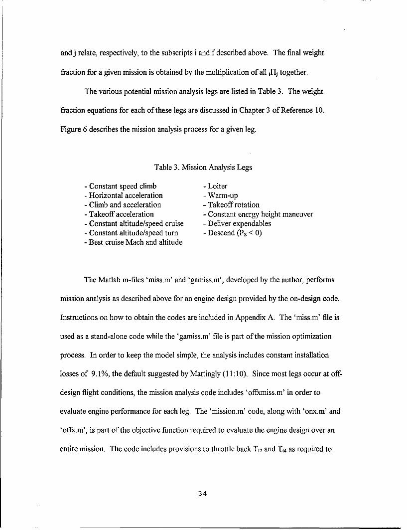
The various potential mission analysis legs are listed in Table 3. The weight

fraction equations for each of these legs are discussed in Chapter 3 of Reference 10.

Figure 6 describes the mission analysis process for a given leg.

Table 3. Mission Analysis Legs

- Constant speed climb - Loiter- Horizontal acceleration - Warm-up- Climb and acceleration - Takeoff rotation- Takeoff acceleration - Constant energy height maneuver- Constant altitude/speed cruise - Deliver expendables- Constant altitude/speed turn - Descend (PS < 0)- Best cruise Mach and altitude

The Matlab m-files 'miss.m' and 'gamiss.m', developed by the author, performs

mission analysis as described above for an engine design provided by the on-design code.

Instructions on how to obtain the codes are included in Appendix A. The 'miss.m' file is

used as a stand-alone code while the 'gamiss.m' file is part of the mission optimization

process. In order to keep the model simple, the analysis includes constant installation

losses of 9.1%, the default suggested by Mattingly (11:10). Since most legs occur at off-

design flight conditions, the mission analysis code includes 'offxmiss.m' in order to

evaluate engine performance for each leg. The 'mission.m' code, along with 'onx.m' and

'offx.m', is part of the objective function required to evaluate the engine design over an

entire mission. The code includes provisions to throttle back Tt7 and Tt4 as required to

34

ensure the available thrust is equal to the required thrust. Moreover, the code can

evaluate the final WTO (with the method described below) and determine the feasibility of a

maximum Mach, maximum altitude leg.

onx.m dataM°, CTO

s Yes

e o pRun engine at missionI =0.091 point power (offxmiss.m)

Calcula tee t rmine Fgma, F, S

Run ngine at m ission point rrq(Offx-m ,

/ ~ I . 9 I ,--

No

Srun engine at mission point FreqN (°ffx'm) tdermnS

TSFC =S/(1 -)Calculate (il-

Figure 6. Mission Analysis Flow Chart for a Leg.Adapted from Fig 6.E3 (10:209)

Takeoff Gross Weight (WTo Determination

As part of the optimization process, the value for WTO has to be updated as the

fuel weight Wf varies, since changes in Wf directly affect WTO. The three methods

35

developed in this study to update WTO are described below. It must be realized that the

weight models and the mission analysis code are based on fixed values of wing loading,

WTo/S and thrust loading, TsIJWTo.

The first approach investigated is valid for all aircraft and is discussed in more

details in Reference 8. In this method, as a first step, the WTO value selected for the

mission analysis is compared with

WTO(r)W +(rmc w ,) (10)=w,

WTO

where

WTo(r) = WTo as a function of empty weight fraction (lb)

Wp = total payload weight (lb)

rmc = remaining fuel coefficient = % of Wf remaining on landing

WTO = present value of WTO as provided to the mission analysis code (lb)

F = empty aircraft weight fraction, WE/WTO

F is tailored to a given aircraft type and is further defined as (10:70):

F = MaWTO(mss (11)

where

M = material modifier

a,b = coefficients determined by the type of aircraft

36

The coefficient a and b are determined by experience for a given aircraft type and

have no specific physical meaning. Since one of the aircraft investigated in this study, the

Short Range Interceptor, is a combat aircraft built with advanced materials, values for M,

a and b are selected as 0.9, 2.34 and -0.13 respectively (10:70,80).

If WTO(miss) WTo(r), then the right value for WTo has been obtained. If not,

additional iterations of the mission analysis, with new estimates for WTO(i,,), are

performed until convergence. The author found that a good way to estimate WTO(m.j) for

successive iterations was to use this relationship:

estimate WTO(iss) = (WTO(mss) + WTo(r))/ 2 (12)

The method described above was found to be inadequate for larger aircraft, such

as the Global Strike Aircraft. It was noted that any variation in Wf larger than a few

hundred pounds from one GA generation to the next would make WTo diverge to either

zero or infinity due to the highly non-linear behavior of Equation (11).

In order to correct the limitations of the weight model described above, a second

approach, based on data from Table 8.2 from Reference 4, was developed for the GSA

using the following linear relationship between WTO and Wf:

WTOGSA = 1.3138634Wf + 39621 (13)

37

It must be noted that Equation (13) is only valid for the GSA and that a new WTO

model would have to be developed for aircraft which do not fit the models described

therein. It must be noted that the two weight models described above are not depended

on a given aircraft empty weight. The final WTo obtained from optimization run using

these models can be used to help determine the lowest possible aircraft structural weight.

A third WTO model was developed in order to investigate means to accelerate

gross weight convergence and reduce the dependence of the WTo convergence scheme on

aircraft data. This additional scheme use fuel weight as a ninth design variable,

i.e. x9 = Wf. This new variable is a dummy variable which is not a part of the engine

design as such. This x9 = Wf variable is used to determine an individual WTo for every

design and to ensure the gross weight does not diverge to the infeasible mission region.

The side constraints boundaries for x9 are defined by the user and are based on available

data or experience. The gross weight for each design investigated by the global optimizer

is determined as follows:

WTO = Wempty + Wfdes (14)

where

W~pty = Aircraft takeoff weight without fuel.

Wfd. = dummy fuel weight variable = x9

Wpty includes the weights of the structure, avionics, payload and engines. A

good estimate of this value can be obtained from available aircraft data. A constraint is

also applied to ensure that only the gross weight does not diverge upward:

38

Wf___ Wfdes (15)

where

Wf= mission fuel weight as determined by the mission analysis program

If x9 is properly bounded by side constraints, Equation (15) ensures that Wf will

stay below the upper fuel weight boundary and thus keep WTO from diverging upward.

This method was investigated with the SRI. It must be realized that since Wmpty is

constant, this weight model is more applicable to engine retrofit situation since the aircraft

structural weight is not adjusted as Wf varies.

Aircraft Cost Model

One of the objectives to minimize as part of the optimization process is the aircraft

cost. The cost model is a term of the global objective function. The model used is a

simple approximation based on empirical data (16) and defined as follows:

Costg/c = Cl.FSL.Nng + C 2 + C 3.Ws (16)

where

Costkc = total aircraft cost ($)

C, = engine cost coefficient ($/lb uninstalled thrust)

C2 = avionics cost ($)

C3 = airframe Cost coefficient (%/lb aircraft empty weight)

FSL = uninstalled thrust at sea level static per engine (lb)

39

Ws = aircraft structural weight (lb)

Neng = number of engine

CI, C2 and C3 are constants derived from experience. Typical values for C1 and C3

are between 60 and 120 $/lb, and 500 to 700 $/lb respectively (16). C2 values depend on

the function of the aircraft and covers a wider cost range. The variable Ws needs to be

broken down further:

Ws = WTO- Wf- Wp- WA- Weng (17)

where

WTo = aircraft takeoff weight (lb)

Wf = fuel weight (lb)

Wp = total payload weight (lb)

WA = avionics weight (lb)

Weng = engine weight (lb)

It is necessary for the airframe designer(s) to provide values for WTO initial, WA

and Wp. The last term of Equation (17), Weng, is determined as follows (16):

W., = NeFSL ( W en, / M . ) (18)

40

where

mo = engine mass flow (Ibm/s)

The parameter (We,,g/mo) represents the specific engine weight and is a indicator of

an engine relative size. A typical value of 8 for this parameter will be used for this

project (16). It must be realized that for the weight convergence model based on

Equations (14) and (15), Ws is essentially a constant term in Equation (16), since the

values of Wmp, WA and Wp are fixed.

The cost model discussed above is crude and should not be considered accurate to

determine aircraft cost. This is so because this model does not include such important

aspects of overall system costs such as research and development, logistic support or the

use of state of the art technology and materials. This model should eventually be replaced

by a more accurate and complex cost model or computer code. However, an accurate

estimate of the aircraft cost is not important at this point, as one only needs to determine

the relative cost of each design. The main purpose of including cost is to explicitly allow

for the possible direct tradeoff of aircraft cost and engine performance as measured by the

total fuel usage over a mission. For this reason, the cost model used in this study is

considered adequate for the problem at hand.

Engine Annulus Area Model

The third objective to achieve as part of the optimization process is to ensure the

engine is as small as possible. In this project, it is achieved through the minimization of

41

the inlet annulus area Aa, as it is a good indicator of engine size (13:section 10-4). The

annulus area corresponds to the area of the inlet where the airflow goes through, i.e. the

annular area between the hub and the tip of the first stage fan rotor. From this point

onward, this area will be referred as the inlet area. The area model presented below is

described in details in Reference 13, section 10-4. A, is defined as follows:

Aa = hubr 1 (19)\ tip

where

A. = annulus area (ft2)

rtip = radius at tip of the first stage fan rotor (ft)

rhub/rtip = hub to tip ratio

In terms of engine performance parameters, the specific thrust (FsL/mo)is expressed

as follows:

FsL - FSL FO (20)m0 mospecA(0

From Equation (20) an expression for A, in terms of engine performance can be

derived:

Aa = m FsL ° (21)mOspecC(FsL inO)

42

where

0 = static temperature ratio

5 = static pressure ratio

m0 C = (m40)/(5A.) = specific flow (lbm/sec-ft2)

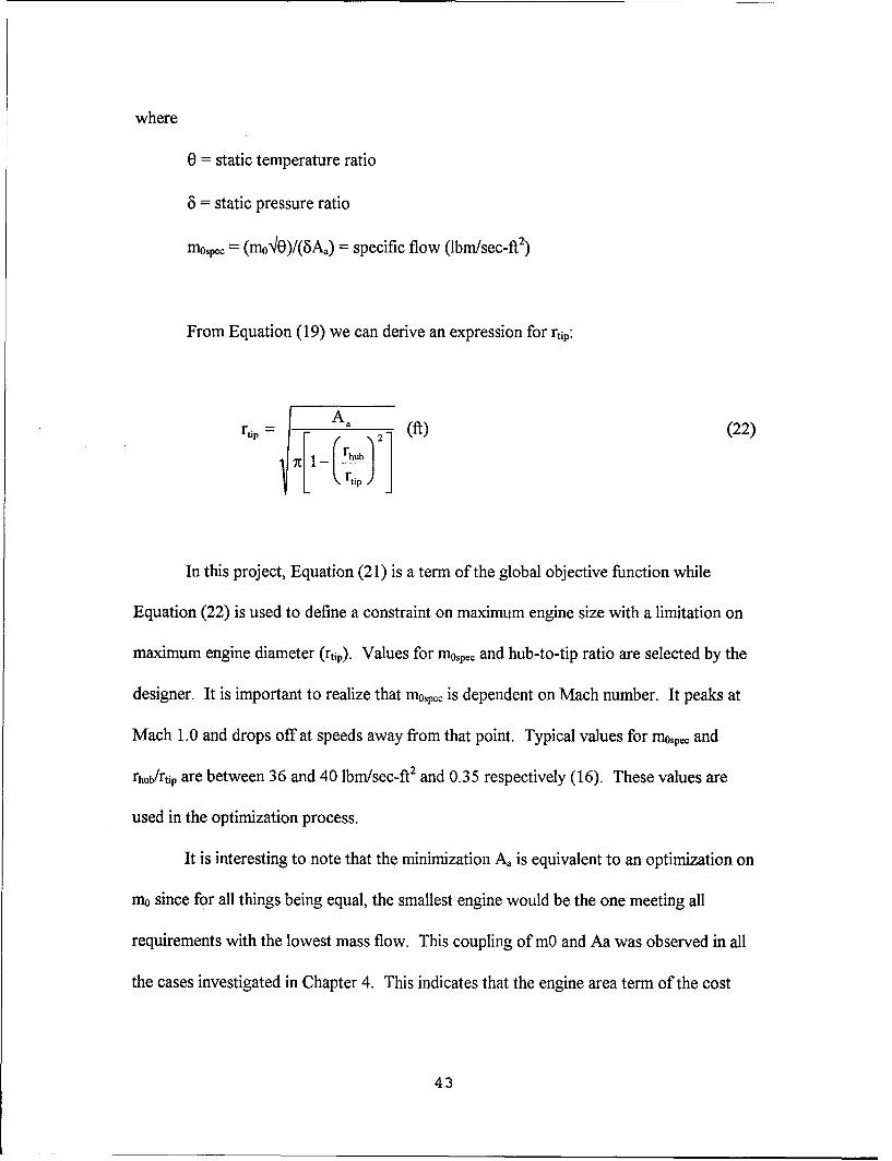
From Equation (19) we can derive an expression for rtip:

rtip " A (22)

7C1

In this project, Equation (21) is a term of the global objective function while

Equation (22) is used to define a constraint on maximum engine size with a limitation on

maximum engine diameter (rtip). Values for mospec and hub-to-tip ratio are selected by the

designer. It is important to realize that mospp is dependent on Mach number. It peaks at

Mach 1.0 and drops off at speeds away from that point. Typical values for mospc and

rhub/rtip are between 36 and 40 lbm/sec-ft2 and 0.35 respectively (16). These values are

used in the optimization process.

It is interesting to note that the minimization Aa is equivalent to an optimization on

m0 since for all things being equal, the smallest engine would be the one meeting all

requirements with the lowest mass flow. This coupling of mO and Aa was observed in all

the cases investigated in Chapter 4. This indicates that the engine area term of the cost

43

function could be replaced by the value for mo with virtually no effect on the final design.

A,, could then be evaluated as part of the final performance calculations for the optimal

design.

Miscellaneous Constraint Equations

As part of the optimization process, constraints must be imposed for PO, TO,

spools rpm and the specific work for the high pressure turbine stage (Aht/y). Constraints

on Pt3, Tt3 and rpm are imposed due to material stresses considerations. The turbine

specific work constraint is discussed in more details below.

The expression for the aforementioned variables are as follows:

Compressor Exit Pressure (10:Ch 4):

Pt3 = (PoIr-lIdIl'IcsIcH)/ 144 (23)

where

Pt3= compressor exit pressure (psi)

Po = freestream pressure (psi)

IT = isentropic freestream recovery pressure ratio

fld = diffuser pressure ratio

l-i' = fan pressure ratio

I ,H = high pressure compressor pressure ratio

44

Compressor Exit Temperature (10:Ch 4):

Tt3 = TOtrx.CtH (24)

where

Tt= compressor exit temperature (R)

To= freestream temperature (R)

,r = isentropic freestream recovery temperature ratio

T,, = fan temperature ratio

cH = high pressure compressor temperature ratio

Low Pressure Spool Rpm (12):

RPM1 = 100 cH 0 T r (25)[,R TOR TrR

where

RPM1 = rpm low pressure spool (% of on-design rpm)

R = subscript referring to on-design values of the appropriate variable

High Pressure Spool Rpm (12):

RPM2 = 100 cH 0 - r 'T C' (26)

45

where

RPM2 = high pressure spool rpm (% on-design rpm)

High Pressure Turbine Specific Work (16):

Ah-- T 1 (4J (27)Shv CptTt41lt Ia-I~t 7, T_ (27)

where

Aht/W = high pressure turbine specific work (BTU/lbm)

x = Normalized high pressure turbine inlet temperature (Tt4/TsL)

Cp,= specific heat at constant pressure downstream of burner (BTU/Ibm-R)

Tt4= burner exit temperature (R)

iltH= high pressure turbine efficiency

yt = ratio of specific heat downstream of burner

The constraint on Aht/w is imposed because of aerodynamics considerations.

Since, in Equation (27), Cpt and TSL are constants and since rjt does not vary much over

the allowable 1IFt range, it turns out that Ilt is the critical variable in the determination of

the high pressure turbine specific work. This implies that Equation (27) is essentially a

constraint on the high pressure turbine pressure ratio. Historical data suggest that for

state-of-the-art engine, the practical lower limit for -ltHis of the order of 0.35. Below this

value, major shock losses and flow separation occurs, thus limiting the maximum work

46

that can be extracted by a single high pressure turbine stage (16). This lower limit of Ilt

translate into a value for Aht/V of the order of 32 BTU/Ibm. This was the value used for

this study. The practical upper limit for flR is approximately 0.52, a value beyond which

the high pressure turbine might be unchoked (8).

Global Strike Aircraft and Short Range Interceptor

In this section we introduce the sample aircraft used to evaluate the performance

of the SQP and GAs in finding optimum engine designs. The aircraft selected are the

Global Strike Aircraft and a short range interceptor. The descriptions of both aircraft

include general overviews of their roles, typical mission profiles, and the parameters values

and constraints used in this thesis.

Global Strike Aircraft (GSA). The GSA is a new aircraft concept under study at

Wright Laboratories. It is described in detail in Reference 4. It is a very long range

stealthy attack aircraft designed to takeoff from friendly bases, preferably in the

continental United States, far away from the battle zone and then fly at high altitude to

take out specific targets with highly accurate standoff guided munitions. A typical mission

would involve flight over 5000 nm in supersonic cruise at altitudes on the order of 60,000

ft. It is an interesting aircraft to study because the level of engine performance required

for this aircraft is based on forecast of propulsion technology available by the year 2025.

The mission profile is presented in Table 4, while the data necessary for the optimization

process is included in Table 5. The GSA drag profile is included in Appendix B.

47

Table 4. Global Strike Aircraft Mission Profile (4)

Leg Altitude (fi) Mach Number Comments

1. Warm up, Taxi 0 0 Idle2. Takeoff 0 0.4 Takeoff distance: 3,600ft,

Mil power3. Accelerate to 0 0.4-0.8 MuI power

climb speed4. Climb and 0-60,000 0.8-1.5 Mil power, minimum

accelerate to fuel pathsupercruise

5. Outbound 60,000 1.5 Part mil power,supercruise distance 5,000nm

6. Combat6a. Weapon 60,000 1.5 Part mil power

launch sweep6b. Launch

Weapons6c. 7200 turn 60,000 1.5 Mil power, turns at 1.5g

7. Return supercruise 60,000 1.5 Part mil powerdistance 5,000nm

8. End loiter and 0 Best Endurance Mach Part mil power, Loiter atland 30,000 ft

landing distance 3,600 ft

Most of the general data and constraints information included in Table 5 were

obtained in Reference 4 and 16. Most of the engine parameters are the default values

proposed by Mattingly (10:116, 125). A few of the selected values, however, require

further elaboration. The Ki weight factors are set to one, thus giving each of the

objectives (fuel consumption, cost and weight) an equal impact on the design. Values of

Cl and C3 were set at 60 $/lb FSL and 500$/lb WE respectively to represent the state of the

art (16). The values for hf, e,,, em, bleed air fraction, riA and the Pt5' constraints were set

48

in Reference 16. The fl constraint was set to keep both the high and low pressure

turbines choked (8).

Table 5. Global Strike Aircraft Optimization Data (4,10,16)

General Data Engine Parameters Constraints

K, 1 Cpr = 0.238 BTU/lbm-R Tt4 4,460 RK2 = 1 CPt = 0.295 BTU/Ibm-R T 7

< O R (no AB)K3 =1 c = 1.4 m0 < 500 lbm/sC1 = 60 $/lb thrust t = 1.3 0.2 ___M5 < 0.7C2= 40,000,000 hf = 18,400 BTU/Ibm AHT/O _< 32 BTU/lbmC3 = 500 $/lb WE Cooling air #1 = 0.05 0.2 _< M5, < 0.95Wen/mo = 8 Cooling air#2 = 0.05 Spools RPM 110%ro, = 40 lbm/sec-ft2 [IB= 0.97 Cost < 150,000,000 $rhwbrtip = 0.35 IlDl. = 0.97 rtip < 4 ftWro initial = 259,500 lb IIN = 0.98 1 _< a!__ 3Wfinitial = 167,345 lb ee,= 0.91 3 <l-', 8.5Wp = 16,440 lb eh =0.9 80:5 17 < 100WA = 3,180 lb etH= 0.89 [ItL< 0.5WpE = 16,440 1b etL = 0.91 P, > Pt5No of engines = 4 e.-= 0.99 Takeoff distance 3,600 ftrmc = 0.05 e.L = 0.99 Pt3< 2,000 psiTsL/WTO = 0.391 evro = 0.99 Tt3 2,2600 RWTo/S = 51.77 lb/ft2 rAB= 0.95 FSL 25,343 lbKI and CDo = Appendix B yAB= 1.3 Wf< 175,000 lbK2 = 0 CpAB= 0.295W, = 92,155 lb Hnnx max = 0.97

Po/P9 = 1Bleed air = 0.005IlA= 0.9671b = 0 .9 8

Short Range Interceptor (SRI). The short range interceptor is a hypothetical

concept investigated by the author as part of a term project for conceptual engine design

class. It is a small, high thrust and highly maneuverable fighter aircraft with supercruise

49

capability optimized for air combat. The conceptual engine design for this aircraft has

been performed in detail using the trial-and-error process outlined in Chapters 1 to 7 of

Reference 10. As the SRI engine cycle parameters had been obtained through the trial-

and-error optimization process described at Reference 10, the short range interceptor

engine represent a good baseline case to evaluate the performance of the GA optimization

process. The SRI typical mission profile is presented in Table 6. Table 7 lists the

optimization data for this aircraft and Table 8 describes the optimum cycle and flight

parameters previously obtained by the author. The SRI drag profile is included in

Appendix B.

The discussion about the values found in Table 7 is similar to the GSA case with

two exceptions. First, the values of C1 and C3 were set at 90$/lb FSL and 600$/lb WE

respectively to represent advanced technology that is not yet as the level of the GSA.

Second, all the engine parameters were set at Mattingly's proposed default values.

50

Table 6. Short Range Interceptor Mission Profile

Leg Altitude (ft) Mach Number Comments

1. Warm Up, Taxi 2000 0 Idle2. Takeoff 2000 0.2 Takeoff distance: 1,500ft,

max power3. Accelerate to 0 0.2-0.7 Mil power

climb speed4. Climb and 0-30,000 0.7-0.9 Mil power

accelerate tocruise altitude

5. Accelerate to 30,000 0.9-1.5 Mil powersupercruise

6. supercruise 30,000 1.5 Mil power,distance 250nm

7. Launch - -

AMRAAM8. 360o, 5g turn 30,000 1.6 Max power9. 2 x 3600 turns 30,000 0.9 Max power10. Combat 30,000 0.8-1.6 Max power

acceleration11. Fire AIM-9, gun - -12. Escape Dash 30,000 1.5 il power

distance 25nm13. Return subsonic 30,000 0.9 Part mil power

cruise distance 200nm14. Loiter 10,000 0.41 Part mil power15. Land 2000 0.2 landing distance: 1,500 ft

Maximum Mach/ 50,000 2.5 Max powermaximumaltitude leg

51

Table 7. Short Range Interceptor Optimization Data

General Data Engine Parameters Constraints

K, = 1 p 0.238 BTU/lbm-R TW4 3,2000 RK(2 = 1 C~ = 0.295 BTU/lbm-R Tt7 3,6000 RK(3=1I yc= 1.4 mo ! 270Olbm/sC = 90 $Ilbthrust yt= 1.3 0.2 M5 O .6C2 = 5,000,000 $ hf = 18,000 BTU/lbm AHT/O 32 BTU/lbmC3 = 600$/lb WE Cooling air #1 =0.05 0.2: M5 , 0.95Weng/flo = 8 Cooling air#2 =0.05 Spools RPM5 110%

mp,,= 37 lbmlsec-ft2 FIB = 0.97 Cost 30,000,000 $rh~b/rtip = 0.35 I-D, = 0.97 rtip 2 ftWTo initial = 24,800 lb I-IN = 0.98 0.2:! a:5 1.0Wf initial 7,997 lb e,,, 0. 89 3 ! rl, 5Wp =2,6341lb e~h 0. 9 24 Iv 30WA= 1,000lb eH0.89 ntI!! 0.5WPE=1,234 lb eL 0.91 Pt 5'> !POTsL/WTO = 1. 14 eH= 0.98 Takeoff distance:< 1,500 ftWTo/S = 65 lb/ft2 e = 0.99 Pt3 375 psiNo of engines = 1 e.PTO =0,9 8 Tth ! 1,660- Rrmc = 0.02 rjB 0.97 FSL 2!27,523 lbM = 0.9 (material modifier) yA = 1.3 Wf 5 10,0001ba =2.34 CpAB= 0. 295b = 0.13 Fj, max =0.971(1 and C~o= Appendix B P0/P9 = 1K2 = 0 Bleed air =0.01

W t = 16,803 lb FIB = 0.9611b =O. 9 8

52

Table 8. Trial-and-Error Process Short range Interceptor Optimum Design

At design point:

Mo = 1.6 h = 35,000 ft mo = 204 lbm/s FSL max= 11,199 lb

IL = 22.5 I'l, = 3.7 c = 0.6 FSL mil = 22,365 lb

Tt4 = 3,200 R Tt7 =3,600' R M5 =0.35 CTO= 0.016

Sea-level performance:

Mo= 0 h = 0 ft mo = 261 ibm/s FSL max = 30,926 lb

I-L= 26.3 [I', = 4.18 cx = 0.56 FSL mil = 19,776 lb

Tt4 = 2,968' R Tt7= 3,600' R M5 = 0.356 CTO = 0.016

53

III. Methodology

Introduction

This chapter describes in details the objectives of this thesis, the methods used to

achieve them, the most significant hurdles that were met during the project, and how those

hurdles were circumvented. The on-design and mission analysis optimization processes

will also be covered, as are the main assumptions that pertained to the thesis.

Objectives

The overall objective of this thesis was to perform a multidisciplinary and

multiobjective constrained optimization of mixed stream, low bypass turbofan design.

The optimization approaches had to cover on-design engine optimization at specific flight

conditions and engine optimization over a whole mission for a given aircraft.

To achieve the main goal stated above, several sub-objectives had to be met as

follows:

1. Include aspects of multidisciplinary optimization with the use of on-design

and off-design cycle analysis, which are based on thermodynamic principles, and

the inclusion of mission analysis, which involves aspects of aerodynamics such as

drag and lift.

54

2. Apply principles of multiobjective optimization with the minimization of

engine size and fuel usage, and overall aircraft cost. The different objectives were

to be weighted properly with linear scaling.

3. Develop codes to perform on-design, off-design, and mission analysis for a

mixed stream, low-bypass turbofan and adapt them to be part of a global objective

function.

4. Develop automated approaches to perform on-design engine optimization

and engine optimization over an entire aircraft mission.

5. All codes are to be Matlab m-files to create a package that is readily

transferable from one operating system to another and which achieves a high level

of modularity.

Assumptions

The methods used to achieve the objectives mentioned above were based on the

following assumptions:

1. Both the low and high pressure turbines remain choked for a feasible

solution.

2. Components' efficiencies are considered constant.

3. Installation losses are set to a constant 9.1%.

4. The engine exhaust mixer is of constant area, i.e. A5 / A5 is constant.

55

5. As/A 8 R is constant and is equal to one, i.e. the exit nozzle has a fixed

throat.

6. Basic aircraft data such as TsL/WTo, WTo/S, drag profiles, and an initial

value for WTO are available.

7. The aerodynamic coefficient K2 is set to zero since both the Global Strike

Aircraft (GSA) and the Short Range Interceptor (SRI) are high performance

combat aircraft assumed to have uncambered wings (10:39).

8. The reference flight condition for engine optimization over a whole mission

is sea-level static.

9. The convergence of WTo as Wf varies is accomplished as part of the genetic

algorithm optimization only. It is assumed that fuel weight, and hence WTo, will

vary little during the local optimization process. The purpose of this assumption is

to ensure that the local optimizer remains well-behaved.

10. High-temperature effects on CP and Cv are neglected to allow the use as-is

of the engine models described in Reference 10. This affects only the GSA since

the technology used for this aircraft allows very high turbine temperatures.

11. Other on-design and off-design analysis assumptions are as stated in

Chapter 2.

Optimization Problems Statements

This thesis attempted to resolve three different types of optimization problems.

The first type was on-design multiobjective engine optimization at a given flight condition.

56

The second type was multiobjective optimization over a whole mission. For these two

types, an objective function of the form shown in Equation (28) below was chosen to

depend explicitly on the system parameters of fuel consumption, aircraft weight, and

engine inlet annulus area. The third type was single-objective optimization over a whole

mission. This last type was a sub-case of the second type. It was used to compare

optimization results with the design and performance data previously obtained by the

author and to investigate the impact of the aircraft cost and engine annulus area sub-

objectives. The problem statement for each type are described below.

Type 1. Multiobjective on-design optimization at a given flight condition.

Maximize:

F(x) = KisS + K2sCost + K3sArea (28)

where

F(x) = global cost function

x = design variable vector: x, = compressor pressure ratio, I-,

x2 = fan pressure ratio, 11-,

X3 = high pressure turbine inlet temperature, Tt4

x4 = afterburner temperature, Tt7

x5 = bypass ratio, (x

57

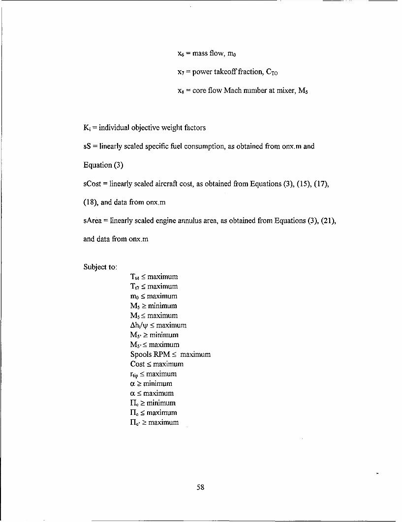
x6 = mass flow, mo

X7 = power takeoff fraction, CTO

X8 = core flow Mach number at mixer, M5

Ki = individual objective weight factors

sS = linearly scaled specific fuel consumption, as obtained from onx.m and

Equation (3)

sCost = linearly scaled aircraft cost, as obtained from Equations (3), (15), (17),

(18), and data from onx.m

sArea = linearly scaled engine annulus area, as obtained from Equations (3), (21),

and data from onx.m

Subject to:Tt4 - maximumT17 < maximummo < maximumM5 > minimumM5 < maximumAht,/ -< maximumM5 > minimumM5 , < maximumSpools RPM < maximumCost < maximumrtip! _ maximuma >_ minimuma<5 maximumFI - minimum11 ,2 maximum[I, >_ maximum

58

H-It < minimumItL< 0.5

Pt5, > PtPt3 < maximumTt3 < maximum

Type 2. Multiobjective engine optimization over whole mission:

Maximize:

F(x) = KxsWf + K2sCost + K3sArea (29)

where

sWf= linearly scaled mission fuel usage as obtained from miss.m and

Equation (3)

Subject to:

Same constraint as Type 1 aboveTakeoff distance _< maximum

Moreover, for a design to be considered feasible, it must accomplish the whole

mission by not failing any legs, and the maximum Mach/maximum altitude leg, which is

usually not part of the mission profile, must also be flown successfully. The best engine is

thus the design that meets all mission requirements with the lowest fuel usage, engine size

and aircraft cost.

59

Type 3. Single-objective engine optimization over whole mission:

Maximize:

f(x) = sWf (30)

Subject to:

Same constraints as Type 2 above, except for the cost and engine

radius constraints, which are ignored

Type 3 is a sub-case of Type 2 and it is used to compare the results generated by

the optimizer with those obtained earlier by the author and to investigate the impact of the

aircraft cost and annulus area sub-objectives.

Cases Investigated. Engine optimization was performed to test the validity of the

overall optimization processes and their related engine and optimization computer codes

on various cases as follows:

Case 1. A simple three-leg mission with the SRI used to test the Type 2

optimization process, since it ran considerably faster than a full fledge mission

(hours vs. days). The mission profile is described in details in Chapter 4.

60

Case 2. Type 1 on-design optimization performed with the SRI at Mo = 1.5 and

h = 30,000 ft. This case was used for comparison with the design presented in

Table 8 in order to investigate the difference between on-design and full-mission

optimizations. The flight conditions were selected because the aircraft spends the

majority of the mission at or near those conditions. For this case, only the

minimization of the specific fuel consumption was considered to allow comparison

with the original results presented in Table 8.

Case 3. A Type 3 optimization with the SRI that used a complete 19-leg mission.

and with a maximum Mach/maximum altitude leg. This was the case used to

compare the overall optimization algorithm with data previously obtained by the

author using the trial-and-error process mentioned in Chapter 2. Constraints on

Pt3 and Tta at the design point were ignored to ensure that Case 3 was performed

under the same conditions as the original case mentioned above. The value for

mospec was set to 37 lbm/sec-ft2 for the same reason.

Case 4. A Type 3 optimization performed with the GSA that included the 19-leg

mission. This case was compared with Case 5 to investigate the impact of the size

and engine annulus area sub-objectives and to investigate the behavior of the GSA

gross weight determination model.

61

Case 5. A type 2 optimization performed with the GSA, fully constrained, and

with a 19-leg mission. This case was selected as a case study by Wright

Laboratory.

Case 6. Type 1 optimization performed with the GSA at M0 = 1.5 and

h = 60,000 ft for comparison with Case 5. The reasons to do so are similar to

those of Case 2.

The outputs of each case include the design variables values for the best design, all

the outputs listed in Table 1, and, if applicable, values for WTO, Wf, aircraft cost and

annulus area. The results for these cases are presented and discussed in Chapter 4.

Overall Approach Taken to Achieve Thesis Objectives

The thesis objectives were achieved with the completion of the following steps,

which are described in details in later sections:

1. Creation of the engine on-design analysis computer code.

2. Creation of the engine off-design analysis computer code.

3. Creation of the mission analysis computer code.

4. On-design engine design optimization with global genetic algorithm (GA)

and local gradient-based optimizer.

62

5. Full-mission engine design optimization with global GA and local gradient

based optimizer.

The main drive of the project was not to create new tools but to use existing

methods, such as GAs and engine performance analysis, together in novel ways in order to

automate engine conceptual optimization. Hence a major aspect of the work

accomplished in this thesis consisted in building interfaces between on-design, off-design

and mission analysis codes with both the GA optimizer and the local gradient-based

optimizer. This implied that all the computer codes used had to be modified in order to

work together seamlessly, with minimal user input, to perform the overall optimization

process. The modifications to the codes affected the way data are transferred between

programs but not how their respective outputs were determined.

All the codes used and written for this thesis are available and can be obtained by

following the instructions included at Appendix A. The instructions on how to set up a

problem and perform an optimization run are included in Appendix C.

Matlab as a Programming Environment. As mentioned earlier, it was decided to

use Matlab to program all the required codes and perform the optimization. The reasons

for this choice are numerous. Matlab is a powerful mathematical application which can

efficiently perform large numbers of iterative calculations. Matlab comes with its own

simple and user-friendly programming language which does not require compilation to run

programs. Moreover, many optimization routines are included as part of the Matlab

63

optimization toolbox and many more are available from various educational institutions'

Web sites.

Matlab executable files all use the '.m' extension and are commonly referred as m-

files. These file can be simple batch files or complex mathematical subroutines. The main

advantage of the m-files system is its inherent modularity. It allows the substitution of

subroutines in a program by the simple change of a word in the program. This modularity

is crucial to this thesis as this allows for growth of the overall optimization algorithms.

For example, advanced installation losses or cost models could be created as m-files and

included in the original objective function file.

Another advantage of Matlab is that the language used is Matlab, and not

operating system, specific. This means that any m-file will work without modification on

any computer with a functional copy of Matlab. For example, an m-file written on a Unix

machine would work just as well on a DOS machine. The only exception to this is that m-

files names for DOS machine can be no longer than eight characters long. The codes used

in this thesis were designed for a Unix environment and, as a results of this, some m-files

names are longer than eight characters. They would thus require some modifications to

run under DOS.

Creation of the On-Design Analysis Computer Code

The on-design analysis code created by the author for this thesis is used as part of

the on-design optimization objective function and also as part of the off-design and

mission analysis. It is based on the theory and approach covered in Chapter 2.

64

To perform the analysis, the code requires as input a 1 x 8 array with the value of

the eight design variables (1-1, l'Ic,, Tt4, TOT, X, M0, CTO, and M5 respectively). The

program then initializes the engine parameters (such as efficiencies and flight conditions)

and evaluates the altitude properties at the given flight conditions. The program performs

on-design calculations and, as the last step, sets the results obtained as reference values to

be used by the off-design code. All the engine parameters are included as part of the on-

design code. The altitude properties, such as air pressure and temperature, are calculated

with an m-file at altitude up to 65,000 ft, using equations developed in Chapter 1 of

Reference 2.

The program was made robust to ensure viable answers were provided, even for

unfeasible points. This was required for use with the optimization routines, since

unworkable values, such as imaginary numbers or division by zero, would make the

optimization process fail. Those problems were averted by ensuring Pt5'/Pt5 and Pt9/P9

values were greater than one. This was accomplished by the assignment of values greater

than one to those parameters if the case arose where those conditions were not met. A

flag inside the program was also set to indicate that a point failing one or more of the

above conditions was unfeasible. A similar technique was used to ensure values for M

were real numbers. The accuracy of the program was tested using examples and data

from Chapter 4 of Reference 10.

The stand-alone on-design code, 'onx.m', required two major modifications to be

used as part of the optimization process. First, the program was turned into a Matlab

function. A Matlab function is like a Fortran subroutine in that it only accepts specific

65

inputs and produce outputs. This was necessary to ensure any on-design analysis

performed as part of the optimization would not be corrupted by parameters values from

earlier function calls or other codes. The second modification involved the inclusion, as

part of the on-design code, of the global objective function parameters and linear scaling

data.

The stand-alone on-design code is 'onx.m' while the version used as part of the

optimizer is 'onxopt.m'.

Creation of the Off-Design Analysis Computer Code

The off-design analysis program was developed by the author and is based on the

theory covered in Chapter 2. It is used as a stand-alone program and as an integral part of

the mission analysis.

Inputs for the off-design analysis include the design point (in the same 1 x 8 array

used by the on-design program) and a 1 x 6 array containing off-design conditions (M, h,

afterburner setting (on or off), P0/P9, and starting values for Tt4 and Tt7, respectively). The

code starts by performing an on-design analysis to obtain the reference point parameters.

Altitude properties at the off-design conditions are evaluated in the same manner as the

on-design case. The program then performs off-design calculations, with iterations on tL,

a' and mo required to converge toward a solution. A Newtonian iteration technique

(10:150) is used to obtain ctL so the magnitude of the ttL step size between iterations is

based on a difference between a calculated ctL value and the value obtained from the

66

previous iteration. Iterations on a' and m0 are based on a functional iteration scheme

where the value of the parameter of interest is set to a calculated value until the

convergence criterion is met (10:150). Moreover, as indicated in Figure 4, fixed-step

iterations on ttL are used to keep Pt5'/P5 and M5 , within acceptable limits. If those

precautions are not taken, the equations that defined those parameters would behave badly

and usually fail to converge to a solution. Once component behaviors are determined,

overall engine performance at the off-design conditions is evaluated. The iterative scheme

used in the author's code is largely based on Mattingly's original ONX and OFFX

codes (12).

Another ill-behaved process is the convergence of 'tL, when the difference between

the reference and the off-design value for Tt4 is large, i.e. several hundred degrees. Under

those circumstances, ctL may fail to converge. To remedy this situation, Tt4 is throttled

from the reference value to the off-design in fixed steps. The input value of Tt4 to the off-

design code becomes the 'target value'. The algorithm start with the maximum allowable

value for Tt4, as defined by the user, and throttles from that maximum value to the target

value in small enough steps so as to check and ensure convergence oftL. The step size is

related to the difference between the present iteration Tt4 value and the target value.

Large step sizes are used when the difference is large and smaller ones are used as Tt4

converges to its target value.

An additional feature of the off-design code are the limits set on the compressor

exit pressure (P,3) and temperature (Tt3), and shaft rpm. When upper limits are violated on

those parameters, the program iteratively (with the use of a Newtonian scheme similar to

67

the one used for ctL) throttles back the off-design T 4 until the constraints on these

parameters are met. This implies that off-design performance must be re-evaluated at each

iteration of Tt4.

The off-design analysis code has to be made very robust for the same reasons as

those stated for the on-design case. Off-design parameters have to be evaluated, even for

infeasible points, in order for the mission analysis code to provide a fuel weight value to

the optimizer. Robustness is achieved by the inclusion of the same protections

incorporated in the on-design code, namely protection against infeasible values of Pts,/Pt5 ,

Ptg/P 9, and M. Moreover, if any of the off-design parameters discussed above do not

converge within a set number of iterations, the whole off-design iterative sequence is

aborted and off-design performance is then evaluated using the most recent values of the

components parameters. A flag is then raised to indicate that the given off-design

condition is infeasible.

The stand-alone off-design code is 'offx.m' while the version used in the

optimization process is 'offxmiss.m'. In the 'offxmiss.m' program, on-design analysis is

not required since it is included in the mission analysis code. Penalties are also included in

the program at all points were parameters might fail to converge, i.e. M5, Pt5 '/Pt5, M, Tt,

a', m0, Ptg/Pg, Tt4, Pt3, Tt3, both shaft rpm, and points where the high pressure turbine

might be unchoked (riL > 0.5). These penalties are determined with the use of an

appropriate form of Equation (9) and were added to the global mission analysis objective

function to indicate unfeasible points as discussed in Chapter 2. Since a whole, multi-leg

mission may fail more than one leg, the penalties are calculated in such a way that only the

68

highest value for a given penalty is retained for transmission to the objective function. For

example, if three legs fail to achieve m0 convergence, only the penalty from the leg that

failed to converge by the largest margin is retained.

Creation of the Mission Analysis Computer Code

Again, the mission analysis code used in this thesis was developed from the theory

covered in Chapter 2. The code is used as a stand alone-program and as part of the

mission optimization objective function.

The inputs to the mission analysis code include the same 1 x 8 array used in the on-

design and off-design codes and a mission profile included in an m-file. The mission

profile file contains the number of legs, an array describing each leg of the mission, and the

maximum Mach/maximum altitude leg data, if applicable. The structure of the mission file

is covered in Appendix C.

The program first step is to initialize aircraft data such as WTO, TsL/WTo, WTo/S,

and so on. On-design cycle analysis is then performed at sea level static. The data

obtained from this analysis will be used to determine reference values and the thrust lapse,

T/TSL, for the mission legs off-design conditions. If the design point is not at sea-level

static, the code has the option to evaluate the reference data at the desired point and

perform an off-design analysis at sea-level static to determine FSL. Once the mission

profile is loaded, the initial fuel fraction 03 is set to one and the mission analysis proper is

performed leg by leg.

69

Mission analysis for each leg begins with the input of the leg off-design conditions

from the mission profile. Off-design analysis is then performed to obtain thrust and-fuel

consumption data and also verify the leg's off-design feasibility for the given baseline

engine. Drag parameters K1, K2 and CD0 are then determined from profiles included in m-

files. The drag profiles for the SRI and the GSA are included in Appendix B. The drag

parameters for the SRI are a function of simple linear equations while the GSA drag data

is estimated with a third degree polynomial curve fit from data obtained in Reference 4.

From the drag data and flight conditions, aerodynamic parameters such as CD, drag

and CL are evaluated. Legs where P, = 0, such as cruise, loiter and constant speed turns,

require the reduction of the available installed thrust until it matches the required installed

thrust. In those instances, the required thrust equals the drag. The thrust reduction is

achieved by iteratively throttling back the off-design T17 (if applicable) and Tt4 with the

Newtonian scheme discussed before until the desired thrust is achieved. If it is not

possible to throttle to the desired thrust, an appropriate penalty is applied to the global

mission objective function based on Equation (9) and a flag is raised to indicate an

infeasible solution. The reduction of the available thrust to the required thrust is essential

to ensure that fuel usage is kept to a minimum and to verify that a given engine design can

throttle back far enough to meet all mission requirements. If it is determined that there is

not enough thrust for a given leg, an appropriate penalty is applied and a flag is raised to

indicate an infeasible solution. The weight fraction iHf and the fuel fraction 03 for the leg is

then calculated (10:209). In cases where the values of 03 are too low and diverge to zero

over the mission, 13 is given a set value and a penalty is applied.

70

Once all the mission legs have been analyzed, the fuel weight, Wf, for the whole

mission is determined as are the takeoff distance and the feasibility of the maximum

Mach/maximum altitude leg (if applicable). Again, in cases where the takeoff distance

constraint is not met, an appropriate penalty is applied and a flag is raised. The feasibility

of the maximum Mach/maximum altitude leg is evaluated with the off-design code. If the

point is infeasible for any reason a flag is raised that indicate that this point, and hence the

whole mission, failed. A penalty is applied as described in the off-design code section.

Finally, WTO is re-evaluated with Equations (10), (11), (12) for the SRI, or Equation (13)

for the GSA, and the methods covered in Chapter 2.

The mission analysis program is inherently robust since all the major protections

against design failure are included as part of the on-design and off-design codes. The code

evaluates Wf and the penalties to be included as part the objective function if the design

fails the mission. The application of penalties as part of the mission analysis is of

particular importance to the optimization process. The behavior of Wf when a mission

failed was unpredictable and the fuel weight could jump up or down by as much as a 1,000

lb (for the SRI) between infeasible points. The unpredictable nature of Wf depended

mainly on which part the off-design analysis did not converge for unfeasible points.

However, it was observed these variations in Wf had little impact on the global objective

function values since any irregularities in the behavior of Wf due to unfeasible points were

drowned out by the size of the total penalty, which was typically an order of magnitude

larger than the global objective function value.

71

The mission analysis code was validated using the data and mission profile from

the original SRI data obtained by the author. The process was slow, especially for legs

that required throttling back the thrust, such as low speed cruise and loiter legs. A typical

full mission, such as the SRI 19-leg mission, would require between one and five minutes

to find a solution. The main reason for this slow response is the large number of off-

design performance evaluations required by the code. This number could range in the

hundreds for missions with legs that require throttling back the thrust, such as low speed

cruise.

The stand-alone mission analysis program used in this thesis is 'miss.m' while the

ones used as part of the optimization process are 'gamiss.m' and 'gamiss2.m'. 'gamiss.m'

is used as part of the global optimization while 'gamiss2.m' is tailored for use with the

local optimizer. The main differences between these programs is that 'miss.m' does not

evaluate penalties while 'gamiss.m' and 'gamiss2.m' have no provision to evaluate WTO,

since this calculation is integral to the genetic algorithm as explained below. Also,

'gamiss.m' and 'gamiss2.m' are set as Matlab functions to avoid the corruption of a given

mission analysis with data from earlier iterations.

On-Design Optimization Process

The on-design engine design optimization process at a given flight condition, as

performed in this thesis, involves the use of the on-design analysis code with a genetic

72

algorithm global optimizer and a sequential quadratic programming (SQP) gradient-based

local optimizer. On-design optimization is normally of limited usefulness since an aircraft

rarely flies at the design condition. The reasons this kind of problem was included as part

of the project are threefold. First, since on-design analysis is practically instantaneous

compared to a mission analysis, it was a useful tool for testing programs such as the GA

code and concepts like penalty functions. Second, when performed with a GA, on-design

optimization proved to be a good way to test the robustness of the on-design code since

the GA tries design points all over the design space, or to estimate proper bounds for

design variables. Third, on-design optimization might prove useful in the design of a

weapon system such as a cruise missile, which operates at a given altitude and speed for

most of its flight.

It was decided to use a two-step process to perform the optimization since the size

and shape of the feasible engine design region are difficult to evaluate. This is due to the

complex interactions of the design variables in the determination of on-design calculations.

The first step of the optimization process would consist of a search of the entire design

space with a global optimizer. The purpose of this search would be to identify good

feasible points and improve on them to isolate the best candidates for optimum designs.

The second step of the process consist of a local optimization, performed by a gradient-

based optimization algorithm, with the best designs provided by the global optimizer as

starting points. The purpose of the local optimization is to converge rapidly to the optimal

solution, as gradient-based algorithms are very efficient and converge to a local minima

73

quickly. A genetic algorithm (GA) was selected to perform the global optimization

because a GA is an excellent tool to explore design spaces and locate regions where global

minimas or maximas exist.

The on-design optimization process is controlled by a master program, in this case,

an m-file. This process is illustrated in Figure 7 and is included in the file 'gaondes.m'.

The inputs required for the optimization program are the design variables boundaries, and

the name of the objective function file. Since the sequential quadratic programming (SQP)

optimizer, 'constr.m', uses matrices to compute and store gradient information, the values

of the design variables for each design are scaled to the same order of magnitude. This is

necessary in order to avoid Matlab errors due to badly scaled matrices. For example,

scaling problem might arise due to the fact that CTO is of the order of 0.01 and Tt4 is

expressed in thousands of degrees. The design variables are scaled back to their proper

value as part of the objective function value determination. Additional inputs include the

maximum number of generations and the name of the termination function, if different

than the default parameters. A user defined termination function allows the optimization

to be stopped by a different criterion than the default maximum number of generations.

The default was used for this case.

Once these inputs are received, the genetic algorithm and the objective function are

called and the initial random population is created. The GA used is GAOT, as described

in Chapter 2. The initial population size and the number of generations were left at their

default values of 80 and 50 respectively. This proved more than adequate to obtain good

74

feasible solutions. The best design, as determined by the GA was fed to the SQP local

optimizer, the Matlab's 'constr.m' code described in Chapter 2. Once the local optimizer

has converged to the optimum design, on-design analysis is performed to obtain the

performance data for this point.

Since the GA handles only maximization problems, it was well suited for the

problems at hand, which require the maximization of the linearly scaled objectives for fuel

usage, cost and engine area. However, the value of the local objective function had to be

preceded by a minus sign since the gradient-based optimizer minimizes the objective

function. Moreover, a useful characteristic of GAOT is the variable population size. As

poor designs are weeded out, the population decreases over time and includes only the

best individuals. This has the advantages of speeding up the process because it

considerably reduces the required number of designs to evaluate.

75

- Scaled design variables bounds- Objective function file name (gafunbis.m)I

Global GA optimizer (GAOT)

InitiFn nn-dsign a l

populationFsee ati

[ NoGlobal objective function

(gafunbis.m)

[ Lea °tiizr -- P Lca °jecivTferiminatsri)onu~m

x ~)citersion

yia -es gnnayi

Local~~~salee opiizrLoaatjciviunto

(onxfinal.m)

Final outputs (F, Cost, Area...)

Figure 7. On-Design Optimization Process (gaondes.m)

76

On-Design Objective Function. Since the objective function file evaluates not only

the function value but also constraints information, it requires further elaboration. Every

time the GA optimizer calls the function file, several operations are performed. The

objective function evaluation process is illustrated in Figure 8 and is included in the file

'gafunbis.m'. When the GA transmits a design to the function file, the design values are

converted to their proper values, as described above. The next step involves the

performance of the on-design analysis. With the data obtained from this analysis, the

value of the different terms are calculated and transformed with linear scaling. The

constraint functions are then evaluated and penalties are applied for each constraint that is

not met. Penalties for each constraint are determined with the appropriate form of

Equation (9). The global objective function value is obtained by the addition of all the

individual objectives terms and the subtraction of all the penalties.

The objective function process used as part of the local optimization is similar to

the global case and is illustrated in Figure 9. The main difference resides in the fact that

since the SQP algorithm deals with constraints directly, there is no need for penalty

functions. The on-design optimization local objective function is included in the file

'fun.m'.

Detailed instructions on how to perform on-design engine optimization with the

codes developed for this thesis are included in Appendix C. Although no built-in interface

was created to set-up a case, doing so only requires the modification of three files. The

77

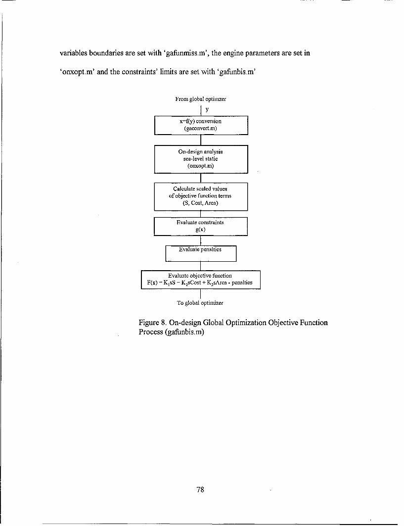
variables boundaries are set with 'gafunmiss.m', the engine parameters are set in

'onxopt.m' and the constraints' limits are set with 'gafunbis.m'

From global optimzer

I y

x=f(y) conversion(gaconvert.m)I

On-design analysissea-level static

(onxopt.m)___7

Calculate scaled valuesof objective function terms

(S, Cost, Area)

Evaluate constraints

F g(x)

I

Evaluate penalties

Evaluate objective functionF(x) - KisS + K2sCost + K3sArea - penalties

ITo global optimizer

Figure 8. On-design Global Optimization Objective FunctionProcess (gafunbis.m)

78

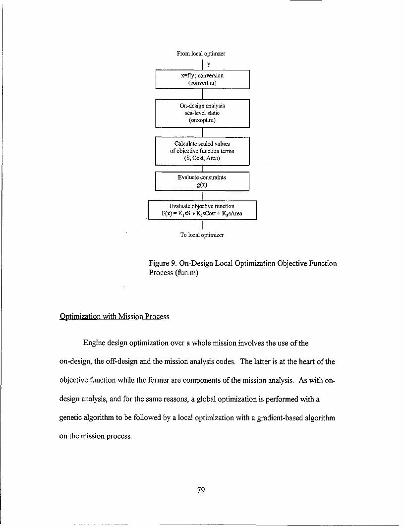
From local optimzer

x=f(y) conversion(convert.m)

IOn-design analysis

sea-level static(onxopt.m)

Calculate scaled valuesof objective function terms

(S, Cost, Area)

Evaluate constraints 1F g(x)

Evaluate objective function

F(x) = K~sS + K2sCost + K3sArea

ITo local optimizer

Figure 9. On-Design Local Optimization Objective FunctionProcess (fun.m)

Optimization with Mission Process

Engine design optimization over a whole mission involves the use of the

on-design, the off-design and the mission analysis codes. The latter is at the heart of the

objective function while the former are components of the mission analysis. As with on-

design analysis, and for the same reasons, a global optimization is performed with a

genetic algorithm to be followed by a local optimization with a gradient-based algorithm

on the mission process.

79

The master file that controls the mission optimization is 'gaoptmiss.m'. The

overall process is illustrated in Figure 10 and 11. The inputs to the optimizer are the same

as the on-design case, i.e. scaled values of the design variable and the objective function

file name. Again, the default termination criterion was used. For this type of

optimization, it was decided to use the default 50 generations for the short range

interceptor and between 25 and 30 generations for the Global Strike Aircraft. The initial

population was set to 100 individual designs. The larger initial population was selected

because the heavy mission and performance requirements usually associated with combat

aircraft tend to severely restrict the feasible design space. A larger population increases

the probability of finding a point in, or at least near, the feasible region. With the inputs

provided, the GA performs the same operations as per the on-design case, with one major

exception. The genetic algorithm for mission optimization used was a version of GAOT

modified to converge toward a final value for aircraft gross weight, WTO. The procedure

selected to update WTO is described in a later part of this section.

Once the GA has operated through the required number of generations, it sends

the three best feasible designs to the local optimizer. Three best points were selected,

instead of only the best design, to ensure that promising solutions were explored. Another

factor is that a good point discovered late in the optimization process might not have been

fully investigated by the GA by the time the termination criterion is met. The selection of

the three best points increases the probability of finding the best solution. If no feasible

solutions are found, local optimization is not performed and the optimization process

8O

stops. This measure is necessary because of the numerous and unpredictable ways a

given design may fail a mission, discussed earlier in this chapter. Because it cannot predict

what variables to adjust (and how to adjust them) to meet the mission constraint, a

gradient-based algorithm would fail to converge to a solution since the gradient

information it produces could not be relied upon.

The local optimizer used for mission optimization is Matlab's 'constr.m'. It has

been modified to accept WTO as an input but it does not perform WTo convergence. WTo

is not updated as part of the local optimization because Wf, and hence WTO, should not

vary significantly since it is assumed that the point provided by the GA is near the local

minima. As a protection against a design becoming infeasible as it is improved by the

optimizer, the value of Wf was multiplied by 1.5 if the mission failed. This encouraged the

local optimizer to stay away from the infeasible mission space.

The last step of the mission optimization is to obtain performance results for all

three points with final calls to the on-design and mission analysis codes.

81

- Scaled design variables bounds- Objective function file name (gafunbis.m)- Termination condition filename (maxGenTerm.m)- Number of generations

T GlobalGA optimizer (ganadon.m, )

SInitial random Ye

p pul tio

Parttio One gnrain

8 2oGlobal objective function(gafumiss.m)

SWTO - Ye Update

Noo~

V3 best points: Yl, y2, y3

To local optimizer (see Fig. 11)

Figure 10. Engine Optimization with Mission Process (gaoptmiss.m) -Part One

82

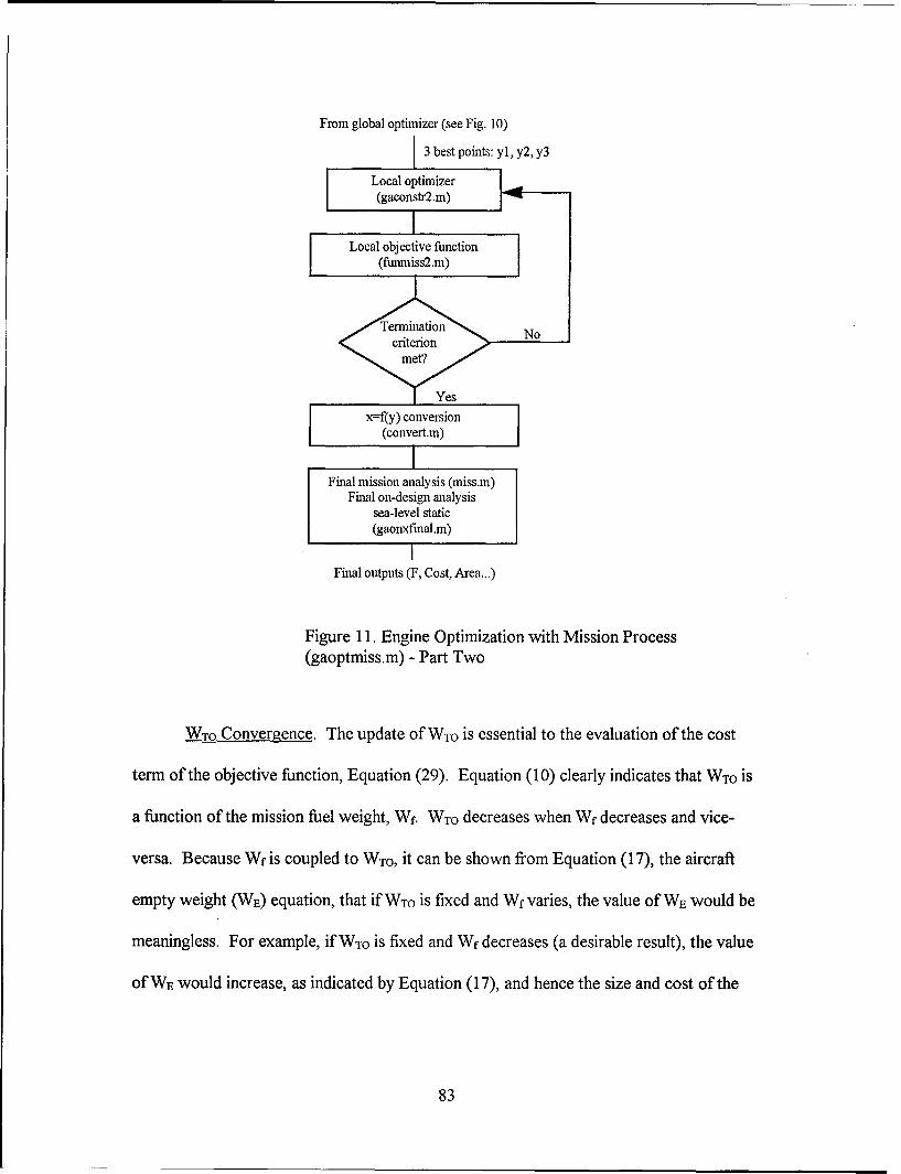
From global optimizer (see Fig. 10)

3 best points: yl, y2, y3

Local optimizer

(gaconstr2.m)ILocal objective function

(funmiss2.m)

x-fRy) conversion

(convert.m)

IFinal mission analysis (miss.m)

Final on-design analysissea-level static(gaonxfnal.m)

Final outputs (F, Cost, Area...)

Figure 11. Engine Optimization with Mission Process(gaoptmiss.m) - Part Two

WTO Convergence. The update Of WTO is essential to the evaluation of the cost

term of the objective function, Equation (29). Equation (10) clearly indicates that WTO is

a function of the mission fuel weight, Wf. WTO decreases when Wf decreases and vice-

versa. Because Wf is coupled to WTO, it can be shown from Equation (17), the aircraft

empty weight (WE) equation, that if WTo is fixed and Wf varies, the value of WE would be

meaningless. For example, if WTO is fixed and Wf decreases (a desirable result), the value

of WE would increase, as indicated by Equation (17), and hence the size and cost of the

83

aircraft would also increase, which is the opposite of the expected behavior for WTo. In

fact, this situation might force the optimizer to diverge away from the optimal design as it

could force the optimizer to maximize fuel weight in order to minimize cost. The update

of WTo as Wfvaries corrects this irregularity.

The determination of a method to allow the convergence of WTO toward its final

value proved to be a major hurdle since the variation of WTo from one generation to the

next might affect the fitness of an earlier design and thus induce instabilities in the GA

behavior. Fortunately, it was observed than once the algorithm converges toward a

solution, WTO would also converge. It was decided for all cases to update WTO at the end

of every generation with the Wf value of the best feasible design of a generation. At the

beginning of an optimization run, WTO is set to a realistic initial estimate as obtained by the

airframe designers. If a feasible point is found for the generation, a new value of WTO is

determined from Equations (10), (11), and (12) for the SRI or Equation (13) for the GSA.

In order to avoid the corruption of future generations with points whose performance

were determined with different values of WTo, the value of Wf for the best point in a

generation was reset to an initial value at every generation until the value of WTO met the

convergence criteria. If no feasible point were found, WTo was not updated since the value

of Wf would be meaningless.

Another problem area was the behavior of WTO when Wf was updated. When Wf

decreased, WTo would tend to diverge toward zero, and in cases where Wf increased, WTO

would tend to diverge into the unfeasible mission region. In order to control the unstable

84

behavior of the gross weight, constraints on minimum thrust and maximum allowable fuel

weight were applied. These constraints effectively set limits for WTO values. Moreover,

to ensure that Wf would not become too high a portion of the gross weight, an additional

constraint was applied as follows:

WTo-Wf > Wmin (31)

where

Wmi,, = minimum aircraft weight without fuel (lb)

W,, is further defined as:

Wfmi, = WS + WA + WP + Wsy (32)

where

Ws = structural weight (lb)

WA = avionics weight (lb)

Wp = Payload weight (lb)

Wsy, = other systems weight (lb)

85

As for other constraints, if the condition of Equation (31) is not met, an

appropriate penalty is applied. At the end of a generation, a convergence scheme to

update WTO in decreasing steps was set up for cases where WTO tends to converge toward

the minimum allowable WTO value. This step was necessary to ensure That WTO would

not be decreased to a value where Equation (31) could no longer be satisfied.

If it is intended to explore potential reductions in structural weight achieved by

more efficient engines, the value of Wfmi. provided to the optimization code can be set to a

value lower than the value calculated with Equation (32). This would allow the optimizer

to, hopefully, further reduce Wf and hence, the gross weight.

There is also a possibility, in situations where WTO increases or with multiobjective

optimization, that the best design might have occurred at a value of WTO different from the

final weight. The impact of a similar situations on the mono-objective cases is reduced,

since the optimum solution tends to be the feasible design with the lowest fuel weight,

regardless of WTO. On the other hand, even for mono-objective optimization, the value of

WTO becomes a factor with heavily constrained missions when variations of WTo might

turn a feasible design into an infeasible one. In order to account for this possibility, the

global optimization codes ensure that the value Of WTO provided to the local optimizer is

the gross weight that was used to determine the best design.

To alleviate some of the limitations and problems mentioned above, another WTO

convergence scheme, based on Equation (14) and (15) and included as part of the global

86

objective function file, was investigated with the full mission SRI case. An appropriate

penalty was imposed when the requirement of Equation (15) was not met. As for the other

design variables, the side constraints for the dummy fuel weight variable, Wfd& , must be set

carefully from previously available Wf estimates. This scheme presents numerous

advantages. It ensure that each design has an individual WTO value assigned to it, thus

eliminating the need to update WTO every generation. This has the potential to

considerably reduce the number of generations required since there is no requirement to

converge WTO over a run because its design is assigned its own value of the gross weight.

Also, there is no need to determine a WTO vs. Wf relationship for a given aircraft since the

only aircraft specific data required is the takeoff weight without fuel. Finally, the problem

with the unstable behavior of Equation (17), as described above, is eliminated since WTO is

always properly matched with Wf.

It is still possible to perform engine optimization for a fixed WTO, if there is a need

to solve such a problem. An example of such a situation would be to investigate how the

payload or range of an existing aircraft could be increased by the selection of an engine

design that provides the lowest fuel usage, Wf. The solution of such a case requires the

removal of the WTO update sequence from the GA and replacing the aircraft cost term of

the objective function (Equation (18)) with only the engine cost CiFsLNng. The procedure

to set up a problem where WTO is constant is described in Appendix C.

87

Mission Optimization Objective Function. Objective function value determination

is governed by the file 'gafunmiss.m' and the process is illustrated in Figure 12. The

function evaluation procedure starts with the conversion of the scaled design variable to

their proper values. The mission analysis function is called upon and evaluates Wf and the

feasibility of the mission for the given design. With the data obtained from the analysis,

the linearly scaled values of the global objective function terms are evaluated. The

constraints are evaluated next and penalties are applied as required.

The penalties for the constraints directly applicable to the design point (i.e. the

constraints listed as part of Equation (28)) are applied in the same way as for on-design

optimization except for the coefficient at the front of Equation (9), which was set to 1.5

instead of 2. This was done in order to give larger penalties to designs that failed the

mission because the mission constraint was considered more critical and difficult to meet.

Since a mission is made of several legs, each of which may fail in several ways, it is easier

for the optimizer to adjust an infeasible point that passes the mission than to do the

opposite. Penalties that arose from a failed mission are calculated with the method

described in the mission analysis section above. Once all the penalties are determined, the

global objective function value is determined and the three best points are updated if

necessary.

The local optimization objective function process is controlled by the file

'funmiss2.m' and it is illustrated in Figure 13. The procedure is similar to the global case.

88

As for the on-design case, the main difference resides in the fact that since the SQP

algorithm deals with constraints directly, there are no need for penalty functions.

From global optimzer

Y, WTO

x-f(y) conversionF(gaconvert.m) 1IMission analysis

(gamiss.m)

Calculate scaled valuesof objective function terms

(Wf, Cost, Area)i

Evaluate constraints

F g(x)IEvaluate penalties

IEvaluate objective function

F(x) KzsWf + K2sCost + K3sArea - penalties

IUpdate 3 best points

and best point

of generation

ITo global optimizer

Figure 12. Global Mission Optimization Objective FunctionProcess (gafunmiss.m)

89

From local optimzer

Iy

x=f(y) conversion

(convert.m)IMission analysis

(gamiss2.m)

ICalculate scaled values

of objective function terms(Wf, Cost, Area)

Evaluate constraints

g(x)

Evaluate objective functionF(x) = K1sWf + K2sCost + K3sArea

ITo local optimizer

Figure 13. Local Mission Optimization Objective FunctionProcess (funmiss2.m)

Engine design optimization with mission proved to be a slow process. A typical

optimization run would take around two to three days for a full mission. It was observed,

however, that a good way to make the optimization process as time-effective as possible

was to properly bound the design variables with the use of side constraints. With

experience, a designer can set limits that will reduce the number of highly unfeasible

points, points that often take longer to solve. One has to be careful not to overconstrain

the design variables to the point where good feasible solutions are excluded from the

design space.

90

Another option available to speed up the process is to replace the initial random

population with population selected by the user. The population thus created must include

the objective function values as well as the design variables values. The advantage of such

a method is to give the GA a population of feasible and near feasible points that would

significantly increase the probability of finding the optimum design. However, this

approach is not recommended since the creation of such a population is itself a time-

consuming process and it defeats the purpose of using a fully automated tool to

accomplish such a search.

Detailed instructions on how to perform engine optimization with mission using

the codes developed for this thesis are included in Appendix C. The set up of a case

requires the modification of four files. The variables boundaries are set with

'gaoptmiss.m', the engine parameters are set in 'onxopt.m', the mission and aircraft

parameters are set in 'gamiss.m' and the constraints' limits are set with 'gafunmiss.m'. A

file containing the drag profile for the given aircraft must also be provided.

91

IV. Findings and Analysis

Introduction

This chapter presents and analyses the results for each of the cases introduced in

Chapter 3. The emphasis is on the behavior of the optimization processes and the related

computer codes.

General Comments and Observations

The overall processes and computer codes for both on-design and mission

optimization proved successful, subject to certain limitations discussed below. The thesis

demonstrated the feasibility of automating engine design optimization.

The engine cycle analysis codes proved very robust and provided acceptable data

to the optimizers in all cases. The genetic algorithm was able to explore the design space

and find feasible designs in five of the six cases investigated. The local optimizer,

successfully converged toward the optimum design when provided feasible points from the

genetic algorithm, although it failed to do so for unfeasible points or near unfeasible points

in two of the six cases.

The six cases investigated were as follows:

Case 1: Test Case with Short Range Interceptor

Case 2: Short Range Interceptor On-design Mono-Objective Optimization

92

Case 3: Short Range Interceptor Mono-Objective Mission Optimization

Case 4: Global Strike Aircraft Mono-Objective Mission Optimization

Case 5: Global Strike Aircraft Multiobjective Mission Optimization

Case 6: Global Strike Aircraft Multiobjective On-Design Optimization

The process for engine optimization with a mission was slow. In these cases, it

took between two and three days of continuous running on a Sun Sparc l0 workstation to

obtain a solution. The main factor that contributed to the lengthy run duration was the

throttling required for cruise and loiter legs. On-design optimization was significantly

quicker, with solutions obtained in less than 30 minutes. The on-design flight conditions

for all mission analysis cases was sea-level static.

It was found that a good way to speed up the codes and to increase the probability

of early entry into feasible space was to properly bound the design variables with the use

of side constraints. The upper and lower boundaries for each variable had to be close

enough to reject the obvious unfeasible points while not being so restrictive as to also

reject good solutions.

Experience and data from on-design and mission optimization runs were used to

gauge variable boundaries. Most side constraints for the design variables were set

arbitrarily, with design variable ranges estimates based on current engine technology and

performance (for the Short Range Interceptor) or on expected future trends (for the

Global Strike Aircraft). Moreover, hard technical limitations might also impose limits to

the range of values available for a given variable. An example of such technological

93

constraint is the value maximum turbine inlet temperature, Tt4, which is dependent on the

properties of the turbine material.

Also of critical importance to ensure the optimizers behaved as predicted was to

carefully set the linear scaling boundaries. If a term of the objective function strayed

beyond improperly set scaling limits, it was observed that the scaled value of the objective

function would undergo a sign change, thus causing the optimizers to diverge and fail.

Scaling limits were imposed very conservatively, again using data from experience and

optimization runs.

The genetic algorithm found feasible points within three generations for all on-

design or mission optimization cases except for the highly constrained short range

interceptor full mission case, for which no feasible point was found. As explained in the

section that covers that case, it is believed that no feasible point existed for this case due

to the engine analysis codes used to solve it. The full mission cases tend to be more

constrained, compared to the on-design cases, due to the numerous mission requirements.

The scheme to select the three best points from the global optimizer for local

optimization proved to be of no value. The solutions provided by the global optimizer

were so similar to each other that they would converge to the same value at the end of the

local optimization. Moreover, in cases where WTo had not converged to a final value,

only one or two points would be provided by the global optimizer. The same would apply

for situations where the global optimizer is near the optimum design and improvement to

the objective function value are sporadic.

94

The techniques used to update the gross weight (WTo) based on Equations (10),

(11), (12) and (13), as described in Chapter 3, proved effective, especially in the case of

the Global Strike Aircraft cases. Although the weight did not converge by the end of a

GSA global optimization run, because the cases were not run for enough generations,

significant reductions in WTO were realized. However, these techniques proved sensitive

and unstable in situations when the initial WTO must be updated upward, in which cases

WTO would diverge into the unfeasible mission region. This divergence was due to the

behavior of the global optimizer, which based its best design points on data from earlier

generations; data that were obtained on WTO values not properly matched to the fuel

weight. Such a situation was encountered in the SRI full mission case. To ensure that

WTO converge properly, it was found that the initial gross weight should be overestimated

in order to ensure it will be updated downward.

Moreover, when WTO is updated, many good points from earlier generations might

become infeasible and this could slow down the optimization convergence. In such a

situation, the SRI test mission usually took between one and five generations to return to

the feasible region and update WTO. It was also observed that the convergence of WTo

toward its final value would take the form of a damp oscillatory motion in the case of the

Short Range Interceptor test case. If WTo did not converge by the end of a run it is

possible that there might still be room to improve the best design at the end of the global

optimization. The remedy to ensure WTO convergence is to increase the number of

generations, at the cost of longer runs. A number of generations between 75 and 100

would seem adequate.

95

The third method to determine WTO, based on Equations (14), (15), and the

dummy design variable x9 = Wfd,, proved extremely effective in the case of the SRI full

mission optimization. Since an individual gross weight is assigned to each design

investigated by the global optimizer, there is no need to update WTO at the end of a

generation. The main advantages of this method are shorter runs, a value of WTo properly

matched with a value of Wf when evaluating aircraft cost (Equation (17)), and the

insurance that WTO will not diverge to the unfeasible mission region. Moreover, no

complex WTO vs. Wf relationship need be determined for a given aircraft since the only

data aircraft specific data required to use the model is the takeoff weight without fuel. It

is felt that this model is superior to the schemes based on Equations (10) to (13).

In cases where the gross weight convergence schemes based on Equations (10)

to (13) were used the cost term of the objective function is of limited validity if WTo fails

to converge. As explained in Chapter 3, viable aircraft cost values depends on WTO

varying in unison with the fuel weight, Wf. Moreover, the aircraft cost term of the

objective function might get worse once the gross weight has converged and is fixed, since

lower fuel weight values increase the aircraft cost as indicated by Equation (17) and its

impact on Equation (16). Although this effect has been observed to be minimal when

compared to the overall benefit of a lower Wf, it is felt that this discrepancy has to be

eliminated with a better behaved cost model. On the other hand, as discussed above, this

situation can be alleviated with the use of a gross weight determination model based on

Equations (14) and (15).

96

Three major constraints drove the selection of the best design by the global

optimizer. The first challenge for the genetic algorithm was to find designs with enough

thrust for all mission legs. The second major constraint to meet involved keeping the high

pressure turbine choked. The third hurdle was to ensure the convergence of 'ti off-

design. The last two constraints were a factor mainly for loiter and maximum

Mach/maximum altitude legs.

In both on-design and mission optimization, the design space appeared to be a flat

region pockmarked with small minimas and maximas. This conclusion was reached with

the analysis of numerous run results. It was found that many designs that varied in

significant ways would give similar values of the objective function. This observation

validates the use of genetic algorithm to search the design space due to the presence of

multiple minimas. However, it raises the possibility of the GA not finding the global

minimum. The only way to ensure the global minimum has been located is by running

cases with a larger populations for more generations.

For the cases investigated, fuel consumption was the factor having the greatest

impact, by far, on the final design. Engine annulus area turned out to be a minor factor

while aircraft cost had negligible impact on the final design. These conclusions are based

on the results presented in Tables 16 and 18 that show that for the GSA, Wf varied by

only 0.21% between the mono-objective and the multiobjective mission optimization cases

(Wf = 110,179 lb vs. Wf = 110,413 lb respectively) while area varied by 1.63% (from

10.41 ft2 to 10.24 ft2). The aircraft cost only decreased by 0.025% (from $97,808,200 to

$97,782,840). The aircraft cost value tended to be low compared to available data (for

97

the GSA) or existing similar aircraft (for the SRI). This was attributed to the crudeness of

the cost model, which cannot account for factors such as research and development.

Further investigation is required to establish the individual impacts of aircraft cost and

engine annulus area in more details.

Case 1: Test Case with Short Range Interceptor

The multiobjective 3-leg mission SRI test case was successful and proceeded

without interruption. The design variables and scaling parameters boundaries are listed in

Table 9. The design and scaling variables side constraints values were based on

knowledge previously gained by the author while performing the SRI trial-and-error

engine optimization. The results and performance for the optimum design are presented

in Table 10. It took about six hours for the optimization codes to converge to a solution.

The mission included two supercruise legs and a 5g turn at M 0.9. It did not include

maximum Mach/maximum altitude leg. Feasible points were found within the first

generation and were improved upon in the next 49 generations. This result was to be

expected as the test case was less restricted than cases with full-mission. The local

optimizer successfully converged to a solution starting from the best solution provided by

the global optimizer.

98

Table 9. Variables and Linear Scaling Boundaries for Case 1: SRI Test Case

Design Variables Boundaries:

24 < l,<30 2.5 < 1-t. < 5 2,900 ° R< Tt4 3,2000 R 3,200 0 R < T17 : <3,6000 R

0.2 -< < 1 250 lb/s < no:m <270 lb/s 0.01 < CTO < 0.02 0.2!9 M 5 < 0.6

Linear Scaling Boundaries:

4,000 lb < Wf< 18,000 lb $10,000,000 <Cost < $30,000,000 3.14 ft2 _< Area < 12.56 ft2

The gross weight, WTO, successfully converged to a final value. The initial WTO

for this case was set to 24,000 lb (vs. 24,800 lb for the final SRI WTO previously obtained

by the author) in order to account for the shorter mission which would require less fuel.

The final value for WTO was 22,394 Ib, which supported the assumption. It should be

noted that WTO was updated only every third or fourth generation and did not converge to

its final value until generation 46. This suggested that the genetic algorithm was able to

improve the best designs throughout the whole run in order to lower the fuel weight and

hence, the gross weight.

99

Table 10. Final Results for Case 1: SRI Test Case

Best point from global optimizer:

fi = 25.4 rI. = 3.16 Tt4 = 2,900' R Tt7 = 3,539.5' R a = 0.73ino = 250.22 lb/s CTO 0.018 M5 = 0.205 Function = 2.0375

Second best point from global optimizer:

He= 25.4 rEl = 3.16 Tt4 = 2,9000 R Tt7 = 3,539.50 R a =0.73mio = 250.22 lb/s CTO = 0.018 Ms = 0.205 Function = 2.0375

Third best point from global optimizer:

rl, = 0 fIl, 0 Tt4 = 0 Tt7 = 0 ,=0

mo = 0 CTO= 0 M5 = 0 Function = N/A

Final design from local optimizer:

rII = 24.65 -I,,= 2.92 Tt4 = 2,900- R Tt7 = 3,519° R aL= 1mo = 250.22 lb/s CTO = 0.01 M5 = 0.306 Function = 2.052

Final performance (sea-level static):

FsLx = 26,872 lb FSLmiI = 15,769 lb Smax = 1.857 (1/hr) Stal = 0.776(1/hr)F/moml. = 107.49 (lbf/lbm/s) F/momil = 63.07 (lbf/lbm/s)itL = 0.413 fIH= 7.81 ritH= 0.3191 PTo = 328,670 WCost = $13,501,000 Area = 6.76 ft2 WTO = 22,394 lb Wf= 6,622 lb

As indicated in Table 10, the global optimizer provided only one point to the

optimizer, and not the three best designs, as would be expected. It should also be noted

that the second best point is identical to the first. This is explained by the fact that WTO

converged late in the run, thus not leaving enough generations to improve on the best

design. The fact that the optimum design did not improve in the last four generations

seemed to indicate that the global optimizer had converged near the global minimum and

that it was appropriate at this point to switch to the local optimizer.

100

Based on experience, the results in Table 10 appear realistic. It was also verified

that all the constraints were met. The local optimizer increased the scaled global objective

function value from 2.0375 to 2.052, which represented a 0.71% improvement. Since the

value of fuel weight Wf was linearly scaled and WTo was not updated for the local

optimization, it is assumed that the improvement in Wf is of the same order of magnitude.

This local design improvement would reduce the final Wf of 6,622 lb by approximately

45 lb.

As seen in Tables 9 and 10, the lower boundaries for Tt4, mo and CTO, and the

higher limit for the bypass ratio, were active. This indicates an even better design might

have been selected if the boundaries for these variables had been expended appropriately,

i.e., decreasing Tt4, mo, and CTO lower limits and increasing the bypass ratio upper limit. It

also suggests that there are significant differences between performance requirements for

the SRI 3-leg and the SRI 19-leg missions, as confirmed by the results from obtained in

Case 3 below.

Case 2: Short Range Interceptor On-design Mono-Objective Optimization

The mono-objective on-design optimization at Mo = 1.5 and h = 30,000 ft for the

SRI was successful and proceeded without interruption. The design variables and scaling

parameters boundaries are listed in Table 11. As it was a mono-objective case, the value

for the specific fuel consumption was not scaled. The results and performance for the

optimum design are presented in Table 12. It took less than half an hour for the

optimization codes to converge to a solution. This case was investigated to see how the

101

on-design solution compared with the full mission design obtained in Table 8. Feasible

points were found within the first generation and were improved upon in the next 49

generations. This result was to be expected since on-design optimization was not heavily

restricted due to the fact that there were no mission requirements to meet. The local

optimizer successfully converged to a solution starting from the best solution provided by

the global optimizer.

Table 11. Variables and Linear Scaling Boundaries for Case 2: SRI On-DesignOptimization

Design Variables Boundaries:

20 < f, < 30 3 <n.. < 4.5 2,9000 R < Tt4 3,2000 R 3,2000 R < Tt7 ! 3,6000 R

0.2 < oc!< 1 190 lb/s:< mo < 230 lb/s 0.01l__CTO:< 0. 02 0.2 _< M5 < 0.6

Linear Scaling Boundaries:

1 (1/hr) < S5 <2.4 (1/hr)

The global optimizer solution was close to the optimal solution since the local

optimizer decreased the value of the fuel consumption by only 0.03% (from S = 1.613 to

S = 1.608). Table 12 also clearly shows that the point provided by the global optimizer

and the final design are very close. The 1-J and CTO constraints were active, which

suggested that these boundaries could have been expanded. The value of Tt7 (3200' R) at

the design flight conditions indicates that the afterburner was off and that there was

enough dry thrust to meet the requirements at these flight conditions.

102

Table 12. Final Results for Case 2: SRI On-Design Optimization

Best point from global optimizer at design point:

l1i = 23.1 I,. =4.5 Tt4 = 3,200° R Tt7 = 3,20 0' R a = 0.2ino = 228.98 lb/s CTO 0.0141 M5 = 0.26 Function = 1.6913

Final design from local optimizer at design point:

flc = 23.2 11; = 4.5 TA = 3,200' R T 7 = 3,2000 R ai = 0.2mo = 220 lb/s CTO 0.01 M5 = 0.51 Function = 1.6908

Final performance (sea-level static):

fI = 26.32 fu. = 4.97 TO = 2,9350 R T 7 = 3,6000 R cc = 0.185mo= 279.1 lb/s CTO=0.0131 M5 = 0.26 FsLmx = 34,971 lbS. = 1.628 (1/hr) F/momx = 125.32 (lbf/lbn/s) fL = 0.4817ricH = 5.297 rHt = 0.379

This point was different than the original design presented in Table 8. Only the

value for Tt4 and rI, are similar. A mission analysis with the full SRI mission was

performed with this final on-design solution. As expected, it failed the mission at several

legs, the first one being the horizontal acceleration. This confirmed the limited usefulness

of on-design optimization to find engine designs that can complete a given mission.

Case 3: Short Range Interceptor Mono-Objective Mission Optimization

The mono-objective 19-leg mission SRI case proceeded without interruption for

50 generations but failed to find a feasible point. No local optimization was performed

103

since the local optimizer could not operate from an unfeasible mission point. This case

was investigated to compare the solution obtained from the automated optimization

process with the one obtained from the trial-and-error method (see Table 8).

The engine and aircraft parameters for this case were set as in Case 1, the SRI test

case. The aircraft cost and annulus area sub-objectives were deactivated. Moreover, the

penalty for failure to achieve ctL convergence was increased to ensure that the optimizer

would stay away from designs that failed this constraint. This protection was necessary

since performance for these designs was unpredictable, it was hard for the global optimizer

to correct the situation, and those designs took by far the longest time to solve. The

penalty for the tL constraint was applied in the same way as all other penalties, with the

exceptions of the coefficient at the front of Equation (9) and the exponent of the same

equation, which were set to 2.5 and 3 respectively.

The design variables and scaling parameters boundaries are listed in Table 13.

After several unsuccessful runs, it was decided to bound the design variable with very

narrow ranges, based on the solution presented in Table 8 in order to increase the

probability of the global optimizer of finding a solution with a small initial population.

This measure was necessary to keep the run time as low as possible. Since the problem

was already heavily constrained by the difficult mission and the maximum Mach/maximum

altitude leg, no constraint were imposed on minimum thrust or minimum weight (Equation

(30)). The best unfeasible design obtained by the global optimizer is included in Table 14.

It took three days for the optimization codes to complete the 50 generations.

104

This case was considered the ultimate test for the optimization scheme developed

in this project. As realized previously by the author, it was a heavily constrained case with

the M = 2.5 and h = 50,000 ft maximum Mach/maximum altitude leg being by far the

most difficult constraint to meet. The 10,000 ft low altitude loiter leg was the other

significant leg to meet. In fact, the search for a design that met these two legs would drive

the whole global optimization process, as it did with the trial-and-error method. The

feasible design space for the SRI full mission case was found to be so restricted that only a

very narrow range of values for the design variables would meet all mission requirements.

For example, the range of possible i,,, as previously investigated, was less than ± 0.1.

Table 13. Variables and Linear Scaling Boundaries for Case 3: SRI Mission Optimization

Design Variables Boundaries, Original Case:

25.6 < 1I < 26.4 4.1 _< rl, 4.2 2,9500 R < Tt4 < 2,9700 R 3,5800 R : Tt7 < 3,6000 R

0.5 <. 0.65 259 lb/s < m0 <263 lb/s 0.014 < CTo <0.017 0.33 < Ms5 0.37

Design Variables Boundaries, Modified Case ( = 2.3):

24 <I-I 28 3.5 <9 H.-, < 4.5 2,9000 R:< T 4 < 3,1000 R 3,550° R < T 7 < 3,600- R

0.45<a0.8 2551b/s <mo<2651b/s 0.013 <CTOo 0.02 0.3 _<M5 < 0.4

7,950 lb < Wfdes -< 8,500 lb

Linear Scaling Boundaries:

6,000 lb < Wf_< 18,000 lb $10,000,000 < Cost < $30,000,000 0.69 ft2 < Area _ 11.02 ft2

The optimization process failed to find a feasible solution because no feasible

solution exists for this case when using the Matlab engine analysis codes developed for

105

this project, for reasons covered in the next paragraph. This conclusion was reached

because the final design presented in Table 8 failed the mission when the reference point

was adjusted to sea-level static. The design from Table 8 successfully passed the mission

when its reference flight conditions were set to their original values of M = 1.6,

h = 35,000 ft. However, when the solution at sea-level static for this engine (obtained

with off-design analysis) was tried as reference point, it failed the mission. The loiter and

maximum Mach/maximum altitude legs were not met because tL did not converge.

Table 14. Final Results for Case 3: SRI Mission Optimization

Best unfeasible point from global optimizer, original case:

1Ir = 25.92 n, = 4.12 Tt4= 2,959.20 R Tt7 = 3,582.80 R o = 0.51mo= 259.6 lb/s CTO = 0.0167 M5 = 0.338 Function = -2.7362

Best point from global optimizer, modified case (Mm-- 2.3:

ro = 26.13 I-, = 4.02 TO = 3,039' R T 7 = 3,558.7' R a = 0.652mo = 263.71 lb/s CTO = 0.013 M5 = 0.359 Function = 0.8132

Final design from local optimizer, modified case (M- a, :

no = 26.23 11o = 4.01 Tt4= 3,003.60 R Tt7 = 3,555.10 R a = 0.652

mo = 263.97 lb/s CTO= 0.01 3 M5 = 0.359 Function = 0.8152

Final performance, modified case (max = 2.3, sea-level static):

Mo0, = 2.3 hma, = 50,000 ftFsLn,,x = 30,737 lb FSLmid = 19,306 lb S.. = 1.733 (1/hr) Smil = 0.849(1/hr)F/moma = 116.44 (lbf/lbm/s) F/m il = 73.14 (lbf/lbm/s)fl-tL = 0.419 H.,H = 6.533 Il- = 0.352 PTo = 450,040 W

Cost = $14,472,000 Area = 7.13 ft2 WTO = 25,171 lb Wf= 8,306 lb

106

As mentioned above, small variations in the engine analysis calculations performed

by the codes developed by the author and the calculations obtained from the ONX, OFFX,

and MISS programs, are believed to account for the failure of the original design when

the reference conditions are taken as sea-level static. Examples of potential variations are

the different altitude models used and the more relaxed convergence criterion in

'offxmiss.m'. These differences in calculations become a factor because the ranges for the

design variables at M = 2.5 and h = 50,000 ft are very narrow. Moreover, as mentioned

before, the design space for this case is very restricted, even when using Mattingly's

codes. This means small variations in calculations at sea-level may have a large enough

impact at the maximum Mach/maximum altitude leg flight conditions to turn a feasible

design into an infeasible one.

This hypothesis was confirmed with the performance of an off-design analysis at

the original SRI reference point of 35,000 ft and M = 1.6 with the sea-level static design

from Table 8 as reference point. The results of this analysis are presented in Table 15,

along with the original design values from Table 8. It can be seen that, as expected, the

design variables values obtained with the codes developed in this study are practically the

same as those provided in Table 8. However, the small differences between the original

values and the calculated values were enough to make the design obtained from the off-

design analysis fail both the loiter and maximum Mach/maximum altitude leg.

107

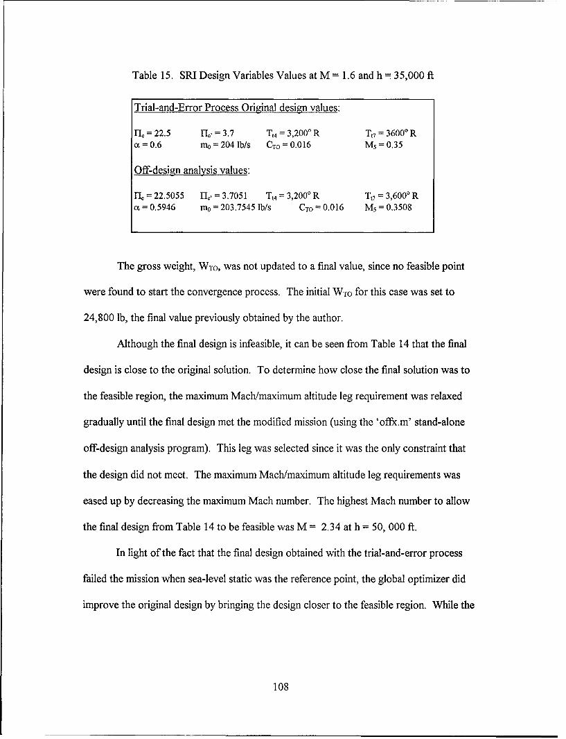
Table 15. SRI Design Variables Values at M = 1.6 and h = 35,000 ft

Trial-and-Error Process Original design values:

ri. = 22.5 r,. = 3.7 Tin = 3,200' R TO = 36000 Ra = 0.6 mo =204 lb/s CTo = 0.016 M5 = 0.35

Off-design analysis values:

i, = 22.5055 n..' = 3.7051 Tt4 = 3,2000 R T 7 = 3,600' Ra = 0.5946 mo = 203.7545 lb/s CTO = 0.016 M5 = 0.3508

The gross weight, WTO, was not updated to a final value, since no feasible point

were found to start the convergence process. The initial WTO for this case was set to

24,800 lb, the final value previously obtained by the author.

Although the final design is infeasible, it can be seen from Table 14 that the final

design is close to the original solution. To determine how close the final solution was to

the feasible region, the maximum Mach/maximum altitude leg requirement was relaxed

gradually until the final design met the modified mission (using the 'offx.m' stand-alone

off-design analysis program). This leg was selected since it was the only constraint that

the design did not meet. The maximum Mach/maximum altitude leg requirements was

eased up by decreasing the maximum Mach number. The highest Mach number to allow

the final design from Table 14 to be feasible was M = 2.34 at h = 50, 000 ft.

In light of the fact that the final design obtained with the trial-and-error process

failed the mission when sea-level static was the reference point, the global optimizer did

improve the original design by bringing the design closer to the feasible region. While the

108

original design failed both the loiter and the maximum Mach/maximum altitude leg due to

ttL convergence, the solution provided by the optimizer only failed the maximum

Mach/maximum altitude leg because the low pressure turbine might have been unchoked.

Moreover, even though the optimization code did not find a solution, it provided useful

design information by clearly indicating which part of the mission could not be met and

why.

Modified SRI Full Mission Optimization. Based on this above information,

Case 3 was retried with a maximum Mach requirement reduced to Mmax = 2.3. This case

was investigated to see how the optimizer would behave with a feasible but very restricted

case. The number of generations was set to 25 and the design variable bounds were

expanded, as indicated in Table 13, to allow the search of a larger design space.

This case failed when a WTO convergence model based on Equations (10), (11),

and (12) was used because the gross weight diverged upward until no feasible designs

could be found. This occurrence demonstrated how sensitive this weight convergence

method is to the initial WTO value.

On the other hand, this case was resolved successfully with the use of the WTO

determination method based on Equations (14) and (15). A feasible design was found at

generation 2. Although the local optimizer was able to improve the best solution from

the genetic algorithm, it oscillated between the feasible and unfeasible, which might

suggest it was close to failure. A seen from Table 14, the improvement on the objective

function value was 0.25%, from 0.8132 to 0.8152. The behavior of the local optimizer is

109

due to the fact that the final solution was very close to the unfeasible mission region as it

was noted that only a small range of designs would prove feasible. This situation would

force the optimizer to step into the infeasible mission region as it tries to update the

design.

The final design and its associated performance is presented in Table 14. It should

be noted that the design and performance of the final engine obtained from the optimizer

are close to the original results presented in Table 8.

As seen in Tables 13 and 14, none of the design variable side constraints were

active, with the exception of CTO which was at its lower limit in both the global and local

solutions. This indicated the variables were well bounded for this case, although the lower

limit for CTO could have been lowered further.

Case 4: Global Strike Aircraft Mono-Objective Mission Optimization

The mono-objective 19-leg mission GSA case was successful. This case was

investigated to provide a comparison baseline for Case 5 (multiobjective GSA), in order to

evaluate the impact of the aircraft cost and engine annulus area sub-objectives. This case

was also useful to determine the validity of the WTO convergence scheme for the GSA

described in Chapter 2. The design variables and scaling parameters boundaries were set

as listed in Table 16, based on data from Reference 16. Since no hard data were provided

in Reference 4, it was decided to set the high altitude turns at 1.5g and the loiter leg at

30,000 ft. These values were selected in order to avoid overconstraining the mission.

With data from Table 7.2 of Reference 4, the minimum weight without fuel, Wmin, was set

110

to 92,155 lb. The results and performance for the optimum design are presented in

Table 17. As it was noticed in test runs that feasible points were found early and that the

gross weight seemed to converge quickly, the global optimizer was set to 25 generations

instead of 50. However, as discussed below, the number of generations should have been

higher. It took two days for the optimization codes to converge to a solution. Feasible

points were found within the second generation.

Table 16. Variables and Linear Scaling Boundaries for Case 4: GSA Mono-Objective

Mission Optimization.

Design Variables Boundaries:

805 <1 !- 100 3 <1I. < 8.5 4,00 0 ' R!9 Tt4 : -4,460' R 0- R!5 T,7 5 0° R

0.5:5 otL <2 400 Ib/s <m 0 5 <470 Ib/s 0.005 5 CTo:< 0.02 0.2: <M 5 5 0.6

Linear Scaling Boundaries:

110,000 lb < Wf < 320,000 lb

As indicated in Table 17, the global optimizer provided only two points to the local

optimizer, and not the three best designs, as would be expected. It should also be noted

that the second best point is nearly identical to the first. The reasons for this situation are

covered in Case 1. The best design did not improve much in the last 3 generations, even

as WTO was updated, indicating that the global optimizer was near the best design and that

it was appropriate at this point to switch to the local optimizer.

111

Table 17. Final Results for Case 4: GSA Mono-Objective Mission Optimization

Best point from global optimizer:

rIL = 80.54 rI'. = 8.13 Tt4 = 4,373.90 R Tt7 = 00 R a = 0.808mno = 416.34 Ib/s Cro = 0.009 M5 = 0.323 Function = 0.99978

Second best point from global optimizer:

rL = 80.54 -L. 8.13 Tta = 4,374.3- R T 7 = 00 R a = 0.808io = 416.34 Ib/s CTo = 0.009 M5 = 0.323 Function = 0.99953

Third best point from global optimizer:

= 0 1.= 0 T 4 = 0 TO = 0 a = 0

mo= 0 CTo =0 Ms = 0 Function = N/A

Final design from local optimizer:

rL = 80.54 1I,= 8.13 Tt4 = 4,374.30 R T 7 = 00 R a = 0.808mo = 416.34 Ib/s CTO = 0.009 M5 = 0.323 Function = 0.99953

Final performance (sea-level static):

FsLni = 42,509 lb Sa 0.8273 (1/hr) F/mow = 102.1 (lbf/lbn/s)ltL = 0.323IH = 9.91 IH 0.32 Pro = 492,621 W

Cost = $97,808,200 Area = 10.41 ft2 WTo = 202,964 lb Wf=110,179 lb

The local optimizer did not improve the best solution from the genetic algorithm

and eventually diverged into the infeasible mission region. The reason for this behavior of

the local optimizer was covered in Case 3. The improvement on the objective function

value was negligible, of the order of x10-10 and the final design was the same as the one

provided by the genetic algorithm. This indicates that the global optimizer had converged

on the final solution.

The gross weight, WTo, did not converge to a final value, although it was close to

doing so. The initial WTo for this case was set to 259,500 lb. The final value for WTo was

112

202,964 lb and it was practically at the lower WTO limit, as determined by Equations (29),

(30), and the minimum Wf limit of 110,000 lb. It should be noted that WTO was updated

every generation until the end of the run at generation 25. This demonstrated that the

genetic algorithm was able to significantly improve the best design throughout the run in

order to lower the fuel weight and hence, the gross weight. It also demonstrated the

advantages of a very high technology engine.

It can be seen that the results presented in Table 17 are of the same order as what

was estimated in Reference 4, although one must keep in mind that high temperature

effects were neglected, as stated in Chapter 3. It was also verified that all the constraints

were met.

The altitude properties algorithms developed as part of the optimization codes,

which were designed for altitude of up to 65,000 ft (the limit of the isothermal layer), were

used for this case, even though the GSA mission included legs at altitude above 70,000 ft.

It was decided to do so since the standard atmosphere table in Appendix B of Reference

10 shows that the isothermal layer could extend up to 80,000 ft, instead of the 65,000 ft

stated in Reference 2.

The aircraft cost of $97.8 million is low compared to the cost of $150 million

estimated in Reference 4. This can be attributed to the crudeness of the cost model, as

explained in Chapter 2. However, as the objective function is only required to minimize

cost in order to find the best engine design, an accurate value was not necessary.

As seen in Tables 16 and 17, none of the design variable side constraints were

active, although the bypass ratio (a) and the compressor pressure ratio (1-) were close to

113

their lower and upper limits respectively. This indicated the variables were well bounded

for this case. The fact that the final fuel weight is so close to its lower limit suggest that a

better design might have been discovered if this limit had been lowered even further.

Case 5: Global Strike Aircraft Multiobjective Mission Optimization

The multiobjective 19-leg mission GSA case was successful and proved the

feasibility of the full multiobjective optimization process for a complex case. This case

was investigated to determine the impact of cost and area on the final engine design, as

compared with Case 4 (mono-objective GSA). This case was set up in exactly the same

way as Case 4, with the exception that the aircraft cost and annulus area sub-objectives,

which were active. Thirty generations were used for the global optimization, instead of

the 25 used for the GSA mono-objective case, in order to ensure WTO had converged.

The design variables and scaling parameters boundaries are listed in Table 18 and they are

again based on data from Reference 16. The results and performance for the optimum

design are presented in Table 19. It took two days for the optimization codes to converge

to a solution. Feasible points were found within the third generation.

114

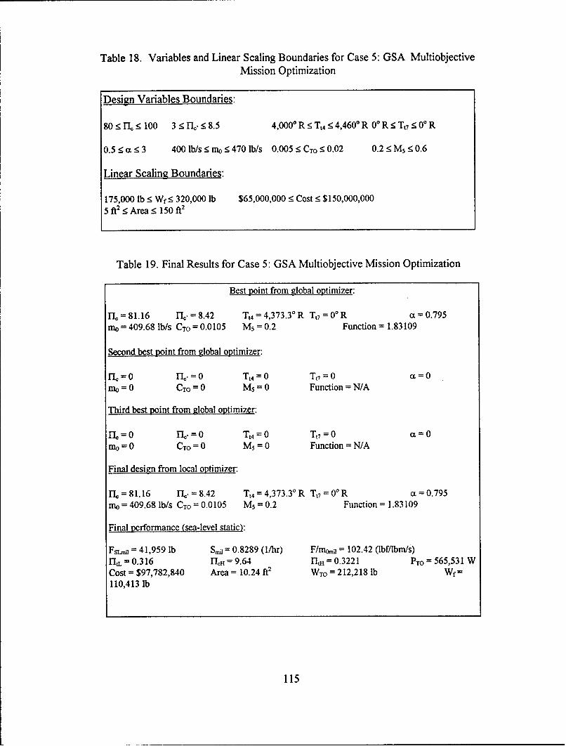
Table 18. Variables and Linear Scaling Boundaries for Case 5: GSA MultiobjectiveMission Optimization

Design Variables Boundaries:

80 < IL< 100 3 <f I, < 8.5 4,000- R:5 Tt4 4,460- R 0- R 5 Tt7:5 0- R

0.5:5 a - 3 400 lb/s:< mo< 470 bs 0.005 < CTo 0.02 0.2:5 M55 <0.6

Linear Scaling Boundaries:

175,000 lb < Wf< 320,000 lb $65,000,000 < Cost < $150,000,0005 ft2 < Area < 150fA2

Table 19. Final Results for Case 5: GSA Multiobjective Mission Optimization

Best point from global optimizer:

n., = 81.16 nr. = 8.42 Tt4 = 4,373.3- R To1 = 0'R a = 0.795mo = 409.68 lb/s CTO = 0.0105 M5 = 0.2 Function = 1.83109

Second best point from global optimizer:

- =0 I .=0 Tt4 =0 TO7 =0 (x=0

mo = 0 CTo =0 M 5 = 0 Function = N/A

Third best point from global optimizer:

1 = 0 'L. =0 Tt4 = 0 To = 0 c = 0mo=0 CTO= 0 M 5

= 0 Function = N/A

Final design from local optimizer:

n. = 81.16 ri. = 8.42 T,4 = 4,373.3° R T,7 = 0°R Cx = 0.795mo= 409.68 lb/s CTo = 0.0105 M5 = 0.2 Function = 1.83109

Final performance (sea-level static):

Fi. = 41,959 lb Sma = 0.8289 (1/hr) F/m = 102.42 (lbf/lbm/s)nd. = 0.316 I'LH 9.64 lIt = 0.3221 PTO = 565,531 WCost = $97,782,840 Area = 10.24 ft2 Wro = 212,218 lb Wf=110,413 lb

115

As indicated in Table 19, the global optimizer provided only one point to the local

optimizer. The reasons for this situation are as discussed in previous cases. The best

design did not improve beyond generation 26, even as WTo kept decreasing, as explained

below.

The local optimizer behaved as in Case 4 and failed to improve the best solution

from the genetic algorithm and eventually diverged into the infeasible mission region.

The improvement on the objective function value was negligible, of the order of xl0"5

and the final design was the same as the one provided by the genetic algorithm. The

reasons for this behavior are explained in the section that covers Case 3 above.

The final value of WTo for the best design was 212,964 lb and the fuel weight was

close to its lower limit of 110,000 lb. It should be noted that this value of WTO was

determined at generation 26 and was not the lowest value for the gross weight. The gross

weight was updated and decreased, to a value of 203,739 lb, until generation 28, after

which the optimizer failed to return to the feasible region in the last two generations. This

result suggests that although genetic algorithm was able to significantly improve the best

engine design, the area and cost sub-objectives limited the potential decrease in gross

weight, since WTo for the multiobjective optimization is 9,254 lb higher than for the mono-

objective case. The impact of these factors is described in more detail below.

With the addition of the aircraft cost sub-objective to the objective function, the

aircraft cost was reduced from $97,808,200 to $97,782,840 between Case 4 and Case 5, a

0.025% decrease.

116

With the application of the area sub-objective, the annulus area was reduced from

10.41 ft2 (see Table 16) to 10.24 ft2, a 1.63% improvement. Since the relative

improvement in area, although small, is two orders of magnitude larger than the

improvement in cost, it is considered that the engine annulus area sub-objective was the

principal cause for the difference between Case 4 and this case. The impact of the area

requirement is illustrated by comparing the values for Wf and WTO obtained for each case

in Table 17 and 19. Wfincreased by 0.21%, from 110,179 lb to 110,413 lb. WTO

increased from 202,965 lb to 212,218 lb, a 4.56% change. The discrepancy between the

relative changes in Wf and WTO are due to the minimum weight constraint imposed by

Equation (31). At WTO = 202,965 lb, the design was very close to fail this constraint and

thus was limited on the potential improvement of Wf. On the other hand, for the case

where WTO is 212,218 lb, this constraint is not as critical as the optimizer had

approximately 10,000 more pounds of gross weight to play with before it hit the minimum

weight constraint. It can also be observed from Table 16 and 18 that the final designs for

Case 4 and Case 5 are similar, although they shows significant difference in their values of

IL, and M5 (6.89 vs. 5.19 and 0.323 vs. 0.2 respectively). This led to a 1.29% reduction

in thrust, from 42,509 lb to 41,959 lb. This reduction in thrust for an increase in fuel

usage indicates that the multi-objective design is not as efficient as the mono-objective

one. However, it is not a critical factor as it was observed that the thrust generated by

these designs was far above what was required to accomplish the mission.

117

It can be concluded from the small difference in performance between the mono-

objective and multiobjective cases investigated that the mission fuel weight has by far the

most impact on the engine final design.

As seen in Table 19, only the M5 side constraint was active. This indicated the

variables were well bounded for this case.

Case 6: Global Strike Aircraft Multiobjective On-Design Optimization

The mono-objective on-design optimization at M0 = 1.5 and h = 60,000 ft for the

GSA was successful and proceeded without interruption. The design variables and scaling

parameter boundaries are listed in Table 20. Several trial runs, including stand-alone off-

design analysis and mission analysis, were required to establish these boundaries at the

design flight conditions. The results and performance for the optimum design are

presented in Table 21. It took less than half an hour for the optimization codes to

converge to a solution. This case was investigated to see how the on-design solution

compared with the full mission design obtained in case 5 (see Table 19). Feasible points

were found within three generations and were improved upon in the next 47 generations.

The local optimizer successfully converged to a solution starting from the best solution

provided by the global optimizer.

118

Table 20. Variables and Linear Scaling Boundaries for Case 6: GSA On-DesignOptimization

Design Variables Boundaries:

60 < 1! <90 2 < H!<4 4,000 ° R:< T 4 < 4,460 ° R 0° R:5 Tt7 < 0' R

1:!9cx < 3 100 lb/s < mo < 300 lb/s 0.01 < CTO < 0.03 0.2 < M5 9 <0.6

Linear Scaling Boundaries:

120,000 lb < Wf< 320000 lb $75,000,000 < Cost < $150,000,0006.2 ft2 !9 Area 5 44.11 ft2

The global optimizer best solution underwent a major improvement when fed to

the local optimizer. The value of the objective function increased by 9.5%, from 1.6215

to 1.7726. Table 21 also clearly shows that the point provided by the global optimizer and

the final design are radically different. The ct, CTO and M5 constraints were active, which

suggested that these boundaries could have been expanded.

A mission analysis with the full SRI mission was not performed with this final

on-design solution since it failed the off-design analysis at sea-level static, the reference

conditions used for comparison with Case 5. This is another clear example where

on-design optimization at a given flight condition is of little help in finding an engine

design that will complete a given mission. The sea-level values are presented in Table 21,

but the data is not to be considered valid since a' did not converge. It can be observed

than most of the sea-level data is unrealistic, with, for example, very low values of 1t, n',

and F/mo.

119

Table 21. Final Results for Case 6: GSA On-design Optimization

Best point from global optimizer at design point:

f1 = 64.2 17G, 2.18 T 4 = 4,293' R TV = 00R = 1.27mo= 103.54 lb/s CTo 0.0293 M5 = 0.439 Function = 1.6215

Final design from local optimizer at design point:

17 = 80.3 n, = 3.11 Tt4 = 4,380' R TO7 = 00 R a=3mo = 101.17 lb/s CTO =0.03 M5 = 0.2 Function= 1.7726

Final performance (sea-level static):

171 = 37.2 [l, = 1.72 TO = 2,970' R T7 = 0° R = 7.08mo = 536.78 lb/s CTO = 0.03 M5 = 0.24 FSLniI = 14,997 lbSa = 0.436 (1/hr) F/momil = 27.94 (lbf/lbml/s) rIL = 0.175rlcH = 21. 6 1 fl, = 0.205

Note: Results at sea-level not valid since design failed at these conditions (see text)

120

V. Conclusions and Recommendations

Introduction

The purpose of this thesis was to develop tools that would automate to a large

extent aircraft engine conceptual design optimization. This goal was accomplished with

the integration of engine cycle and mission analysis with optimization technique such as

sequential quadratic programming and genetic algorithms. Various sample cases such as a

short range interceptor and a global strike aircraft were investigated as proof of concept.

Overall, the objectives stated in Chapter 3 were achieved, for both on-design and mission

optimization, with optimal solutions obtained in all cases investigated. The general

conclusions derived from the thesis results and the recommendations for future work on

this project are presented below.

Conclusions

With the integration of the engine analysis and optimization code under the same

programming architecture, conceptual engine design for on-design and mission

optimization was successfully automated. The optimization process ensured that all

mission requirements and design limitations were met and that the final engine designs

were the smallest, the most fuel efficient, and with the least impact on total aircraft cost.

Since all codes are written in Matlab, which uses a simple language and file

manipulation system, it is easy to modify, improve, and add to the existing codes. This

modularity also makes it relatively simple to expend the engine analysis and optimization

121

tools to include more detail models, such as more advanced installation losses and cost

models.

Although to set up a case only requires the manipulation of a few files, it is a

process prone to mistakes; mistakes that could modify the original codes. Moreover, a

good working knowledge of Matlab is required to manipulate the codes with confidence.

For these reasons, the development of a fool-proof user interface is a must.

The combination of a genetic algorithm (GA) with a local optimizer proved

effective, with the GA exploring a given design space to reach an often limited feasible

region and the gradient based optimizer quickly improving, whenever possible, on the best

solution provided by the GA. Improvement of the objective function value of up to 10%

was achieved by the local optimizer. The use of the three best points from the GA did not

prove useful, since the points were similar and would converge to the same solution by the

end of the local optimization. This dual optimization technique is made even more

important due to the fact that the design space appears to be a relatively flat surface

pockmarked with small minimas and maximas. Constraints were successfully applied to

the GA with the use of penalty functions. The codes developed for this thesis were very

robust, with engine analysis codes that consistently provided usable data to the optimizers,

even for highly infeasible designs.

On-design optimization based on one flight condition worked very well but, as it

was of limited use since a design optimized for a given flight condition would usually fail

other conditions. It was much less constrained than mission optimization, and feasible

points would be found within three generations. The process would typically take less

122

than half an hour to be completed. On-design optimization proved useful to set up

variable boundaries for mission optimization since on-design optimization is a fast process.

The optimization processes developed as part of this thesis were subject to certain

limitations. For one, mission optimization for very constrained mission requirements, such

as a low altitude loiter with a high maximum Mach/maximum altitude leg might not

produce a feasible solution, as in the original SRI full mission case. Moreover, the local

optimizer could not converge to a solution if started from an infeasible, or near infeasible,

mission point. This problem could be alleviated with larger populations and more

generations.

It is of critical importance to properly bound the design variables and the scaling

limits to ensure a faster convergence to a feasible design. This is a process based on

experience and trials runs are often required to determine suitable boundaries.

Another limitation is the possible requirement to setup a gross weight (WTo)

convergence scheme for each different aircraft under investigation. If an improper WTo

model is used, the aircraft gross weight may diverge away from the optimal solution if

WTo is not properly matched with Wf. On the other hand, for the cases investigated, the

WTO convergence schemes proved successful, although longer global optimization run

would be necessary to ensure WTO has fully converged. The WTO determination model

based on Equations (14) and (15), which assign an individual gross weight to each design'

was considered superior to the model based on Equations (10) to (13) since it required

little aircraft specific data. This model was also impervious to gross weight divergence

and would allow considerably shorter runs.

123

A drawback of the mission optimization process is that it is slow, with full-mission

cases requiring between two and three days to converge to a solution, although no user

intervention was necessary during a run. also, it must should be pointed out that the

process involves some major simplifications such as constant installation losses and a

crude aircraft cost model. The cost model used produced low aircraft cost, especially in

the case of the global strike aircraft. On the other hand, since the purpose of the cost

model was to minimize engine impact on aircraft cost and not to evaluate the cost

accurately, the model proved adequate.

Variations of the sub-objective weight factors, Kk, and the individual impacts of

engine annulus area and aircraft cost were not investigated, although it was observed that

fuel weight had, by far, the most impact on the final design. Engine annulus area was a

distant second and the aircraft cost sub-objective had virtually no impact on the final

design. This work is left to future users of the optimization codes.

Despite its limitations and simplifications, it is believed that the tools developed as

part of this thesis are useful as they eliminate a lot of the manual groundwork and

guesswork required at the early stage of conceptual engine design. The concepts brought

forward during this project proved viable, although it is understood that the tools created

to apply them requires further development. The solution provided at the end of the

optimization process should provide a good first engine design which can then be

improved upon.

124

Recommendations

It is believed that further work is required to allow the codes and processes

developed as part of this thesis to reach their full potential as a powerful and versatile

engine optimization tool.

First and foremost, a user-friendly interface must be created to efficiently and

safely enter all the data, parameters, and models (such as cost, WTO convergence, area,

etc.) required to set up an optimization case.

The engine analysis codes, especially 'offxmiss.m', should be reviewed and

modified as required to increase their speed in order to shorten the duration of the

optimization runs. Alternative engine and mission analysis codes could be also integrated

to the existing optimization codes in order to get a faster or more accurate optimization

process. Such codes could be in Fortran or C since Matlab can readily integrate and

process programs written in these languages. As a short term solution to the speed

limitations, cases should be run on dedicated and fast computers. The codes m-files names

should also be modified to allow them to work under a DOS environment.

Advanced models should be created or integrated for engine annulus area, and

especially aircraft cost and installation losses. Development and inclusions of these

models would bring this project closer to a comprehensive engine design optimizer.

The impacts of engine annulus area, aircraft cost, and objective weight factors, Kk,

on the final design should be investigated further with additional runs set up with several

combinations of K1, K2, and K3.

125

Appendix A: Instructions on How to Obtain Optimization and Engine AnalysisComputers Codes

In order to obtain copies of some of, or all, the Matlab computer codes developed

and used as part of this study, contact:

Department of Aeronautics and AstronauticsSchool of Engineering

Air Force Institute of TechnologyWright-Patterson Air Force Base, Ohio

45433-6583

126

Appendix B: Drag Profiles

0.035

0.03

0.025

0.02

0.015

0.01

0.005

0 I I t I

0 0.5 1 1.5 2 2.5 3

Flight Mach Number, MO

Figure 14. CDo vs. Flight Mach Number, M0, for the Short Range Interceptor

0.6

"0.5--

, 0.4

0.3p

0.2

0.1

00 0.5 1 1.5 2 2.5 3

Flight Mach Number, MO

Figure 15. K, vs. Flight Mach Number Mo, for the Short Range Interceptor

127

0.0066

0.0064

0.0062

0.006

o0.0058

0.0056

0.0064

0.0052

0.005 I I I I I I0 0.2 0.4 0.6 0.8 1 1.2 1.4 1.6 1.8 2

Flight Mach Number, MO

Figure 16. CDo vs. Flight Mach Number, M for the Global Strike Aircraft

0.4

e 0.35--

E 0.30Q0

r 0.25

2 0.2

0.15-0 0.2 0.4 0.6 0.8 1 1.2 1.4 1.6 1.8 2

Flight Mach Number, MO

Figure 17. K1 vs. Flight Mach Number, Mo, for the Global Strike Aircraft

128

Appendix C: Engine Optimization Computer Codes Operating Instructions

The purpose of this document is to provide step-by-step instructions on how touse the provided engine analysis and optimization codes. Procedures are included to solvethe following classes of problems:

1. On-design engine optimization at given flight conditions.

2. Engine optimization with mission.

3. Stand-alone on-design engine cycle analysis.

4. Stand-alone off-design engine cycle analysis.

5. Stand-alone mission analysis.

No built-in interface is available to enter variables and parameters. However, theprocess is simple in that it only involves accessing a few Matlab in-files to enter the datarequired to set up a case.

General Comments

All the required codes are included with the disk that comes with theseinstructions. The files have to be downloaded in the same directory. The codes includethe optimizers and the engine analysis codes. The codes have been developed to workwith the Unix operating system. To work under DOS, some files names would have to bemodified to ensure that they are less than eight characters long.

It is assumed that the user has a basic knowledge of Matlab and on how to createMatlab m-files. The user should also be familiar with text editors, such as NEDIT, Vi orWindows' NOTEPAD. The instructions are set for Windows-type environment.

As a reminder, if one desires to disable a function or calculation (such as aconstraint), all that is required is to open the appropriate file and type '%' at the beginningof the desired code line. To see the value of a variable that does not normally appear onthe screen during a run, one must open the file, go to the required line and remove thesemi-colon at the end of the line.

Annex A includes the description of all the variables of interest to the user. AnnexB contains a list of all the m-files used for optimization and engine cycle analysis.

129

It should be noted that any variable with the suffix '_noAB' implies the value ofthe variable when the afterburner is off. The suffix 'of is applied to all off-designvariables and the subscript 'SL' refers to sea-level values.

Updating codes with Fortran or C routines. Matlab has the capability to integrateexternal Fortran or C codes and subroutines. This is a useful feature that allows a user tosubstitute any of the m-file used in the optimization process with his/her own. Forexample, a faster and more accurate existing Fortran off-design analysis code might beused instead of 'offxmiss.m'.

There are two relatively simple way to integrate external codes to a Matlabprogram. The first, and easiest to use, is the shell escape function. With this method theuser write a simple m-file function where the input data are retrieved from a MAT-file(Matlab data storage file format), the Fortran or C code called and executed and theoutput returned to the original MAT-file.

The second approach is more efficient but requires more work since it also requirethe creation of a gateway file to manage input and output data, and the compilation of thefinal routine into a Matlab MEX-file (which is essentially a Fortran or C m-file).

It is not a goal of this document to cover in details the process to create shellescape functions or MEX-files. The detailed procedures necessary to integrate externalcodes are covered in the Matlab External Interface Guide, a manual that comes with theprofessional edition of Matlab.

On-Design Engine Optimization at Given Flight Conditions

This section covers step-by-step procedures to perform on-design optimization.

1. Go to the directory where the optimization and engine codes are.

2. Open a text editor window and start Matlab in another window.

3. Open, in the text editor, the file 'gaondes.m'.

4. While in the above file, set the scaled boundaries for the variable 'y' in the linecalling the genetic algorithm. The example below demonstrates which line to go to andwhere are the positions of each design variable bounds. The values for 'y' are betweenzero and 10, except for y5, the bypass ratio, which can be higher. The conversion betweenthe scaled design variables, 'y', and their proper value, 'x', is as follows:

130

y1"10 = x1 = rley2 1=x=YIcY2 = X2 = H.c'

Y3" 1000 = x3 = T 4

Y4* 1000 = x4 = Tt7

Y5110 = X5 = ay6*100 X6 = MO

Y7/100 = X7= CTOy8/10 = X8= M5

Example:

Y1 Y2 Y3 Y4 Y5 Y6 Y7 Y8

y=ga([2 3;1.5 5;1.5 3.2;3.2 3.6;2 10;1.9 2.2;1 3;2 9],'gafunbis')

5. Save file ('gaondes.m') and close.

6. Open file 'gaonx.m' in the text editor.

7. At the beginning of file 'gaonx.m', set, as desired, the parameters Cp, Cpt, Y, Yt,hp, 61, 62, rib, [Idmax, [-IN, e,, e H, etn, etL, TImPTO, TrnL, 7'm-, 3, IIAB, 7lAB, YAB, Imixmax, CpAB,Po/P 9, M, h,7lb, T3, Pt3, Low and High pressure spools rpms, PTo, K1, K 2, K3, C 1, C2, C3 ,mo,~p, W/mo, and rhub/rtip. Refer to Annex A for the computer code namescorresponding to these parameters.

8. At the top of the second page of file 'gaonx.m', set the boundaries of the linearscaling functions. These boundaries represent the absolute lower and upper limitsexpected for the specific fuel consumption (1/hr), the aircraft cost ($) and the engineannulus area (ft2). See Annex A for the proper variable names. The bndl### boundaryapplies to the most desirable limit while the bnd0##H applies to the least desirable.

Example. If the aircraft cost is expected to fall between $10,000,000 and$30,000,000, then bndlCost = 10,000,000 (since a low cost is desirable) andbnd0Cost = 30,000,000.

9. Save and close file.

10. Open file 'gafunbis.m' in the text editor.

11. At the beginning of the file, set value for WA, Wp, WTo, and Wf. See Annex A forthe proper variable names.

131

12. At the bottom of the first page of 'gafiinbis.m', set the used-defined constraintslimits. All constraints equations are of the form 'ctg# = expression'. The user-definedconstraints equations are as follows, and the values to be set by the user are indicated withbold font:

ctg4 = Pt5primePt5 - Pts'/Pts max;ctg6 = M5prime - Ms, max;ctg7 = - M5prime + MV~ min;ctg8 = ((PO*pir*pid*picprime*pich)/144) - Pa, max (psi);ctg9 = (TO*taur*taucprime*tauch) - T, max (R);ctglO = ((Cpt*Tt4*etath*(1 -(pithA((gammat-1)/gammat))))!(Tt4!5 18.7)) - AHT/O max;

(BTU/lbm)ctgllI - F+ Fmin (lb);ctgl2 = Cost - Cost max ($);ctgl3 = ((Area/((1-(rhubrtipA2))*pi))AO.5) - r max (ft);ctgl4 = Wf - Wf max;ctgl5 = -Wf + Wfmin;

Note: to remove a constraint, just add '%' at the beginning of the constraintequation code line and in front of all code lines of the appropriate penalty 'IF' loop (i.e. infront of 'if..' 'penal# = .',and 'end').

13. Adjust the penalty functions (in 'gafunbis.m') with the constraints values set instep 12 above. The penalties equations are one the second and third pages. The user-defined penalties equations are as follows, and the values to be set by the user areindicated with bold font:

penal4 =(1 .5*((ctg4 + Pt5'/Pts max)!/ Pt5'/Pt 5 max))A12;penal6 = (1.5*((ctg6 + M5, max)!/ M5, max))A2;pena,17 =(1.5*((ctg7+ M5 , min )/ M5 , min))A2;penal8 =(1.5*((ctgg + P, max (psi)) / Pt max (psi)))A2;penal9 =(1.5*((ctg9 + Tth max (R)) / T, max (R)))A2;penallO = (1.5*((ctglO + AHT/O max (BTU/lbm))/ AIIT/O max (BTU/lbm)))A2;penall 1 = ((ctgl 1 + F min (lb)) / F min (lb))A 3;penall2 = (1.5 *((ctgl2 + Cost max ($)) / Cost max($)A2penall3 = (1.5*((ctgl3 + r max (ft))/ r max (ft)))A2;penall4 = (1.5 *((ctgl4 + Wf max)!/ Wf MaX))A2;penall5 = (1.5*((ctgl5 + Wfmin )/!Wfmin))A 2;

14. Save and close file.

15. Open file 'ftm.m' in text editor. Repeat steps 11 and 12. In this file, theconstraints functions are expressed as array value g(x) (instead of 'ctg#=. .. '). If someconstraints are disabled, it is very important to renumber the active constraintssequentially from g(1) to g(k). Save and close the file.

132

16. Open file 'onxfinal.m' in text editor. Set engine parameters as per step 7, thensave and close file.

17. Start optimization process by typing 'gaondes' in Matlab.

18. Once the process is completed, cut and paste all the desired outputs to another file.

Engine Optimization with Mission

This section covers step-by-step procedures to perform engine optimization withmission.

1. Go to the directory where the optimization and engine codes are.

2. Open a text editor window and start Matlab in another window.

3. With the text editor, create a drag profile '.m' file which evaluate KI, K2, CDO andCD for different Mach numbers. For the sake of standardization the file name should be ofthe form 'drag###.m'. See file 'dragsri.m' and 'draggsa.m' for examples of such files.Save and close the file.

4. Create a mission profile m-file with the text editor. . For the sake ofstandardization the file name should be of the form 'leg###.m'.

First, set the number of mission legs with the variable 'nleg'. Second, set themission profile array which contains the type of legs and the off-design and leg parametersfor each leg. The array has dimensions nleg x 14 and uses the following format:

L = [a, bl cl di el fl gi hi ii ji k 11 mi ni;a2 b2 . . . . . . . . . . . . . . . . . . .. M 2 n2;

a8 teg bnIeg .................. nnieg]

where the parameters for L are as follows:

133

ai = leg type codebi = initial Mach number (initial velocity (ft/s) for constant energy height maneuver)ci = final Mach number (final velocity (ft/s) for constant energy height maneuver)di = initial altitude (ft)ei = final altitude (ft)fi = number of g's for turn legs, if applicablegi = number of 360' turns for turn legs, if applicablehi = distance (nm) or time (sec); time in minutes for loiterii = afterburner setting; if zero, AB=0 (off); if one AB=1 (on)ji = expendable weight delivered (lb), if applicableki= angle of descent (deg) if applicableli = Tt4of (R)mi = Tt7of (R)ni= Po/Pgof

The leg type codes are as follows:

1 = constant speed climb2 = horizontal acceleration3 = climb and acceleration4 = takeoff acceleration5 = constant altitude/speed cruise6 = constant altitude/speed turn7 = best cruise Mach number and altitude cruise8 = loiter9 = warmup10 = takeoff rotation11 = constant energy height maneuver12 = deliver expendables13 = descent

Third, Set the variable 'Maxreq' to one if there is a requirement for a maximumMach/maximum altitude leg. Set 'Maxreq' to zero if there is no such requirement. If'Maxreq' is set to one, off-design data for the maximum Mach/maximum altitude leg mustbe provided as follows:

hofmach = maximum altitude (ft);M0ofmach = maximum Mach number;ABmach = afterburner setting for the leg (= 1 if on, = 0 if off)Tt4ofmach = Tt4 for the leg (R);Tt7ofmach= Tt7 for the leg (R);POP9ofmach= P0/P9 for the leg;

Example. A 3-leg mission includes a cruise leg at M = 1.2 and h = 30,000 ft withafterburner off, a 4g turn at M = 0.9 and h = 30,000 ft with afterburner on, and a cruise

134

leg at M = 1.4 and h = 30,000 ft with afterburner off. There is a requirement for amaximum Mach/maximum altitude leg at M = 2.5 and h = 50,000 ft with afterburner on.The mission profile m-file would look like this:

Maxreq=1; % Switch to indicate there is a maximum Mach leg

% Maximum Mach leg off design data

hofmach=50000;M0ofmach=2.5;ABmach=1;Tt4ofmach=3200;Tt7ofmach=3600;POP9ofnach=1;

nleg=3;

L=[5 1.2 1.2 30000 30000 0 0 275 0 0 0 3200 3600 1;6 0.9 0.9 30000 30000 4 2 0 1 0 0 3200 3600 1;5 1.4 1.4 30000 30000 0 0 200 0 0 0 3200 3600 1];

5. Save and close mission profile.

6. Open, in the text editor, the file 'gaoptmiss.m'.

7.' While in the above file, set the scaled boundaries for the variable 'y' in the linecalling the genetic algorithm. The example below demonstrates which line to go to andwhere are the position of each design variable bounds. The values for 'y' are betweenzero and 10, except for ys, the bypass ratio, which can be higher. The conversion betweenthe scaled design variables, 'y', and their proper value, 'x', is as follows:

y* 10 =x l = I'Y2 = X2 = -Ic,

Y3* 1000 = x 3 = Tt4y4* 1000 = x4 = Tt7Y5110 = x5 = a

y6*100 X6 = MOY7/100 = x7 = CTOy/10 = x8 = M5

Example:

Y1 Y2 Y3 Y4 Y5 Y6 Y7 Y8

[y, ... ] = ganadon([2 3;1.5 5;1.5 3.2;3.2 3.6;2 10;1.9 2.2;1 3;2 9],'gafunmiss', ... )

135

8. Save file ('gaoptmiss.m') and close.

9. Open file 'onxopt.m' in the text editor.

10. At the beginning of file 'gaonx.m', set, as desired, the parameters Cp,, Cpt, Yc, yt,hpr, 6 1, 62, lib, lidmax, lIN, ec,, ecH, etH, etL, TImPTO, rimL, 1 mH, 03, HAB, lAB, YB, rlmixmax, CpAB,P0/P9, M0, h,1jb, Tt3, Pt3, Low and High pressure spools rpms, PTO, K1, 1(2, 1(3, C1, C2, C3,mosp., Wng/mo, and rhb/rtip. Refer to Annex A for the computer code namescorresponding to these parameters.

11. At the bottom of the second page of file 'onxopt.m', set the boundaries of thelinear scaling functions. These boundaries represent the absolute lower and upper limitsexpected for the fuel weight (Ib), the aircraft cost ($) and the engine annulus area (ft2).See Annex A for the proper variable names. The bndl### boundary applies to the mostdesirable limit while the bnd0### applies to the least desirable.

Note: optimization with mission is set with sea-level static as the design point.

Example. if the aircraft cost is expected to fall between $10,000,000 and$30,000,000, then bndlCost = 10,000,000 (since a low cost is desirable) andbnd0Cost = 30,000,000.

12. Save and close file.

13. Open file 'gamiss.m' in the text editor.

14. At the beginning of the file 'gamiss.m', set, as desired, the mission and parametersWTo/S, TsL/WTo, CDRTO, aSL, CL.., PTO, rmc, a, b, NLrit, kTo, % installation losses, numberof engines, M, maximum takeoff distance, Wp, WPE, and WA. Refer to Annex A for thecomputer code names corresponding to these parameters.

Note: If the drag profile involves a value of K2 different than zero, insert '%' atthe beginning of the code line '1(2=0'. This code line is at the top of the parameters codelines.

15. At the end of the second page, replace the 'leg###' mission line with the propermission profile file name. The location of this code line in 'gamiss.m' is as follows:

% Calling mission profile using leg###.m% It contains mission legs data and number of mission leg% There is one file per aircraft/mission

legsri c mission profile code line to change to proper mission profile file name

% beginning of mission analysis loop

136

16. Save and close 'gamiss.m'.

17. Open all mission leg files applicable to the current mission profile. The missionlegs and their corresponding files are as follows:

Constant speed climb: 'csspeedclb.m'Horizontal acceleration: 'horizaccel.m'Climb and acceleration: 'clbaccel.m'Takeoff acceleration: 'tkoffaccel.m'Constant altitude/speed cruise: 'csalspcrs.m'Constant altitude/speed turn: 'csalsptrn.m'Best cruise Mach number and altitude cruise: 'bcmbca.m'Loiter: 'loiter.m'Warm-up: 'warmup. m'Takeoff rotation: 'takofrot.m'Constant energy height maneuver: 'csenhgt.m'Deliver expendables: 'delivexp.m'Descent: 'descent.m'

18. On the first page of each applicable leg file, replace the 'drag###' drag profile linewith the proper drag profile file name. The location of this code line in all leg files is asfollows:

% Evaluating Cdo, K1 and CD with the given drag profile drag###.m

dragsri drag profile code line to change to proper drag profile file name

19. Save and close all leg files.

20. Open file 'gafunmiss.m' in the text editor.

21. At the top of the third page of 'gafunmiss.m', set the used-defined constraintslimits. All constraints equations are of the form 'ctg# = expression'. The user-definedconstraints equations are as follows, and the values to be set by the user are indicated withbold font:

ctg4 = Pt5primePt5 - P,'/Pt5 max;ctg6 = M5prime - M5, max;ctg7 = - M5prime + M5 , min;ctg8 = ((PO*pir*pid*picprime*pich)/144) - Pt3 max (psi);ctg9 = (TO*taur*taucprime*tauch) - Tt3 max (R);ctgl0 = ((Cpt*Tt4*etath*(1-(pithA((gammat-1)/gammat))))/(Tt4/518.7)) - AHT/O max;

(BTU/Ibm)

137

ctgl I = - F + F min (lb);ctgl2 = Cost - Cost max ($);ctgl3 = ((Area/((1-(rhubrtipA2))*pi))AO.5) - r max (ft);ctgl4 = Wf,- Wf max;ctgl5 = - Wf+ Wf rmin;ctg16 = - MnWeight + Wmi.

Note: to remove a constraint, just add '%' at the beginning of the constraintequation code line and in front of all code lines of the appropriate penalty 'IF' loop (i.e. infront of,'if...', 'penal# = ... ', and 'end').

22. Adjust the penalty functions (in 'gafunmiss.m') with the constraints values set instep 21 above. The penalties equations are one the third and fourth pages. The user-defined penalties equations are as follows, and the values to be set by the user areindicated with bold font:

penal4 = (1.5*((ctg4 + Pts'/Pt5 max) / Pts'/Pt5 max))A2;penal6 = (1.5*((ctg6 + M5 , max) / MV, max))A2;penal7 = (1.5*((ctg7+ M5 min )/ M5 , min))A2;penal8 = (1.5*((ctg8 + Pt3 max (psi)) / Pt3 max (psi)))A2;penal9 = (1.5*((ctg9 + Tt3 max (R)) / To max (R)))A2;penallO = (1.5*((ctglO + AHT/O max (BTU/Ibm))/ AHT/O max (BTU/Ibm)))A2;penall 1 = ((ctgl 1 + F min (lb)) / F min (lb))A3;penall2 = (1.5*((ctgl2 + Cost max ($)) / Cost max ($)))A2;penall3 = (1.5*((ctgl3 + r max (ft))/ r max (ft)))A2;penall4 = (1.5*((ctgl4 + Wf max) / Wf max))A2;penall5 = (1.5*((ctgl5 + Wf min )/ Wf min))A2;penall6 = (1.5*((ctgl6 + Wmin )/Wmin))A2;

23. Save and close file 'gafunmiss.m'.

24. Open file 'funmiss2.m' in text editor. Repeat step 21. In this file, the constraintsfunctions are expressed as array value g(x) (instead of 'ctg#=...'). If some constraints aredisabled, it is very important to renumber the active constraints sequentially from g(1) tog(k). Save and close the file.

25. Open file 'missfinal.m' in text editor. Set engine parameters as per steps 14 and15, then save and close file.

26. Open file 'gaonxfinal.m' in text editor. Set engine parameters as per step 10, thensave and close file.

27. Open file 'ganadon.m' in text editor. On the first page, right below the comments,set the initial values of the gross weight, the variable 'Wto', and the initial value of thegross weight for the best design, the variable 'Wtobest' (it must be the same value as

138

'Wto'). This step is not necessary if you use a weight model which determine a value ofWTO for each design, as describe in Chapter 2, equations (14) and (15) of the relatedthesis. If such a model is used, a value of takeoff weight without fuel, variable Wempty,must be given at the beginning of 'gaoptmiss.m', 'gafunmiss.m' and 'funmiss2.m'. Theconstraint 'ctgl7' and its related penalty must be activated, as described in Steps 21 and22. Moreover the gross weight models described in Step 28 below must be deactivatedwith 'symbols'.

28. In the same file, on the second last page, set your weight model. It should be anequation for the gross weight, WTO, as a function of the fuel weight, WF. Here are twoexamples of such models, as presently included in 'ganadon.m':

% Wto for GSA

WtoGAM=(1.3138634*Wfmin)+39621; < Weight model for first aircraft

%Wto for SRI

%GAMN4A=M*acoef*(1/(Wtobcoef)); < Weight model for%WtoGAM=(Wp+(rmc*Wfmin))/(1-(Wfmin/Wto)-GAMMA); ' second aircraft

errwto=abs(Wto-WtoGAM);0/ofndata(4)=errwto;

%if errwto> 100,

% For SRI

%Wto=(Wto+WtoGAM)/2;

/oFor GSA

Wto=WtoGAM;

29. Start optimization process by typing 'gaoptmiss' in Matlab.

30. Once the process is completed, cut and paste all the desired outputs to another file.

Cases with fixed WTO. In some cases, it might be desirable to keep WTO constantinstead of updating it as Wf changes. Such a case could be the investigation of the payloador fuel weight difference between engine design. The procedure is the same as describedabove, with the following modifications:

When the linear scaling parameters are set in 'onxopt.m', the boundaries for costhave to be the upper and lower limits of engine cost and not aircraft cost. The scaling

139

limits of all engine (i.e. for a given engine, the scaling values for a twin-engine plane aretwice that of a single-engine one).

- The objective function in the file 'gaftmnmiss.m' must be adjusted for engine cost,not aircraft cost. On the second page of this file, '%' symbols have to be inserted at thebeginning of the code lines 'costa = ... ' and 'costb =.'

- In the same file, the line 'Cost = (C1I*F)+C2+(C3*costb);' has to be changed to'Cost = C1I*F;'.

- The modified portion of 'gafunmiss. m' should look like this:

% Evaluate cost

o/ocosta=-(F*(WengmO))/FmO; <- '%' inserted here/oco stb--Wto -Wf- Wp -Wa-c os ta; <- '%' inserted here

Cost-=C1*F; <= cost term modified here

% Evaluate annulus area

- Modify the file 'ganadon.m' to disable the WTO convergence model. To do soadd % symbols before the required code lines, located in the second last page of the file,as follows:

%if feasible== 1,

%GAMMvA=M*acoef*(1/(WtoAbcoef));%/WtoGAM=(Wp+(rmc*Wfmin))/(1-(Wfmin/Wto)-GAMMA);0/oerrwto=abs(Wto-WtoGAM);0/ofndata(4)=errwto;

%/if errwto> 100,

%/Wto=(Wto+WtoGAM)/2;0/ofndata(1)=Wto;%/lowest=-10;0/ofhdata(2)=-lO;%/Wfmin=-1000000;% fndata(3)=1000000;O/erwo- 10;0/ofndata(4)=errwto;0/ofeasible=0;

140

/ofndata(5)=feasible;/obestl=[O 0 0 0 0 00 0];/obest=[0 0 0 0 0 0 0 0];/obest3=[0 0 0 0 0 0 0 0];

0/ofeasible=0;0/ofndata(5)--feasible;

% end

%/end

Stand-Alone On-Design Engine Cycle Analysis

This section covers step-by-step procedures to perform on-design engine cycleanalysis.

1. Go to the directory where the optimization and engine codes are.

2. Open a text editor window and start Matlab in another window.

3. Open file 'onx.m' in the text editor.

4. At the beginning of file 'onx.m', set, as desired, the parameters Cpc, Cpt, yc, yt, hp,61, 62, lib, fldmax, -IN, e eH, etn, etL, inPTO, IlmL, ImH, 3, [iAB, lAB5 YAB, lmixmax, CpAB,P0/Pg, M0, h, rb, Tt3, Pt3, Low and High pressure spools rpms, PTO, KI, K2, K 3, C 1, C 2, C 3,mospe, Weg/mo, and rhub/rtip. Refer to Annex A for the computer code namescorresponding to these parameters.

5. In Matlab, enter the desired design point as a 1 x 8 array. It should look like this:

x = [xI x2 x3 x4 x5 x6 x7 x8]

where

xl = value for lFix2 = value for I,x3 = value for Tt4x4 = value for T17

x5 = value for otx6 = value for m0x7 = value for CTOx8 = value for M 5

6. Start on-design analysis process by typing 'onx' in Matlab.

7. Once the process is completed, cut and paste all the desired outputs to another file.

141

Stand-Alone Off-Design Engine Cycle AnalysisThis section covers step-by-step procedures to perform on-design engine cycle

analysis.

1. Go to the directory where the optimization and engine codes are.

2. Open a text editor window and start Matlab in another window.

3. Open file 'onx.m' in the text editor.

4. At the beginning of file 'onx.m', set, as desired, the parameters CPC, Cpt, yc, yt, hpr,61, 62, rlb, fldmax, [IN, e,,, eH, etn, etL, TImPTO, lML, "1mH, P, [IAB, T7AB, YAB, f-mixmzx, CpAB,P0/P9, M, h,rjb, Tt3, Pt3, Low and High pressure spools rpms, PTO, K1 , K2, K3, C 1, C2, C 3 ,

m0 p ¢, Weg/mo, and rhb/rtlp. Refer to Annex A for the computer code namescorresponding to these parameters.

5. In Matlab, enter the desired design point as a 1 x 8 array. It should look like this:

X = [XI X2 X3 X4 X5 X6 X7 X8]

where

x, = value for 1,x2 = value for I ,x3 = value for Tt4X4 = value for Tt7x5 = value for otx6 = value for moX7 = value for CTO

xs = value for M5

6. In Matlab, enter the desired off-design conditions as a 1 x 6 array. It should looklike this:

Y = [Yl y2 y3 y4 Y5 y6]

where

yj = value for M, off-designy2 = value for h, off-designy3 = AB setting off-design (= 1, AB on; = 0, AB off)y4 = value for P0/P9 off designy5 = value for T,4 off-designy6 = value for T 7 off-design

142

7. Start on-design analysis process by typing 'offk' in Matlab.

8. Once the process is completed, cut and paste all the desired outputs to another file.

Stand-Alone Mission Analysis

This section covers step-by-step procedures to perform mission analysis.

1. Go to the directory where the optimization and engine codes are.

2. Open a text editor window and start Matlab in another window.

3. With the text editor, create a drag profile m-file which evaluate KI, K2, CDo and CDfor different Mach numbers. For the sake of standardization the file name should be of theform 'drag##4#.m'. See file 'dragsri.m' and 'draggsa.m' for examples of such files.Save and close the file.

4. Create a mission profile '.m' file with the text editor.. For the sake ofstandardization the file name should be of the form 'leg###.m'.

First, set the number of mission legs with the variable 'nleg'. Second, set themission profile array which contains the type of legs and the off-design and leg parametersfor each leg. The array has dimensions nleg x 14 and uses the following format:

L = [ai bl cl di el f, gi hi ii ji k1 1 l n1 ;a2 b2 . . . . . . . . . . . . . . . . . . .. m 2n2;

anleg bnleg .................. nneg]

where the parameters for L are as follows:

ai = leg type codebi = initial Mach number (initial velocity (ft/s) for constant energy height maneuver)ci = final Mach number (final velocity (ft/s) for constant energy height maneuver)di = initial altitude (ft)ei = final altitude (ft)f= number of g's for turn legs, if applicablegi = number of 360' turns for turn legs, if applicablehi= distance (nm) or time (sec); time in minutes for loiterii = afterburner setting; if zero, AB=0 (off); if one AB=I (on)ji= expendable weight delivered (lb), if applicable

143

ki =angle of descent (deg) if applicableli = Tt4of (R)mi= Tt7of (R)ni= Po/P 9of

The leg type codes are as follows:

1 = constant speed climb2 = horizontal acceleration3 = climb and acceleration4 = takeoff acceleration5 = constant altitude/speed cruise6 = constant altitude/speed turn7 = best cruise Mach number and altitude cruise8 = loiter9 = warm-up10 = takeoff rotation11 = constant energy height maneuver12 = deliver expendables13 = descent

Third, Set the variable 'Maxreq' to one if there is a requirement for a maximumMach/maximum altitude leg. Set 'Maxreq' to zero if there is no such requirement. If'Maxreq' is set to one, off-design data for the maximum Mach/maximum altitude leg mustbe provided as follows:

hofmach = maximum altitude (ft);MOofmach = maximum Mach number;ABmach = afterburner setting for the leg ( 1 if on, = 0 if off)Tt4ofmach = Tt4 for the leg (R);Tt7ofmach= Tt7 for the leg (R);POP9ofmach= P0/P9 for the leg;

Example. A 3-leg mission includes a cruise leg at M = 1.2 and h = 30,000 ft withafterburner off, a 4g turn at M = 0.9 and h = 30,000 ft with afterburner on, and a cruiseleg at M = 1.4 and h = 30,000 ft with afterburner off. There is a requirement for amaximum Mach/maximum altitude leg at M = 2.5 and h = 50,000 ft with afterburner on.The mission profile m-file would look like this:

144

Maxreq=1; % Switch to indicate there is a maximum Mach leg

% Maximum Mach leg off design data

hofmach=50000;MOofinach=2.5;ABmach=1;Tt4ofmach=3200;Tt7ofinach=3600;POP9ofmach=1;

nleg=3;

L=[5 1.2 1.2 30000 30000 0 0 275 0 0 0 3200 3600 1;6 0.9 0.9 30000 30000 4 2 0 10 0 3200 3600 1;5 1.4 1.4 30000 30000 0 0 200 0 0 0 3200 3600 11;

5. Save and close mission profile.

6. Open file 'onx.m' in the text editor.

7. At the beginning of file 'onx.m', set, as desired, the parameters Cp, Cpt, y, yt, hp,61I, 62, I-[b, r1-].a, IIN, e,, eta, et, etE, ilmTTO, rimE, lmH, 03, nAB, 11gB, YA, I'Imixmax, CpAB,

Po/P 9 , Mo, hlb, Tt3, Pt3, Low and High pressure spools rpms, PTO, K1 , 1(2, K3, C1, C2, C3,mop, Weg/mo, and rhb/rtip. Refer to Annex A for the computer code namescorresponding to these parameters.

Note: stand-alone mission analysis is set with sea-level static as the design point.

8. Open file 'miss.m' in the text editor.

9. At the beginning of the file 'miss.m', set, as desired, the mission and parametersWTO, WTo/S, TsL/WTo, CDRTO, aSL, CLmx, PTO, rmc, a, b, Mrit, kTo, % installation losses,number of engines, M, maximum takeoff distance, Wp, WPE, and WA. Refer to Annex Afor the computer code names corresponding to these parameters.

Note: If the drag profile involves a value of K2 different than zero, insert '%' atthe beginning of the code line 'K2=0'. This code line is at the top of the parameters codelines.

10. At the beginning of the second page, replace the 'leg###' mission line with theproper mission profile file name. The location of this code line in 'miss.m' is as follows:

145

% Calling mission profile using leg###.m% It contains mission legs data and number of mission leg% There is one file per aircraft/mission

legsri - mission profile code line to change to proper mission profile file name

% beginning of mission analysis loop

11. Save and close 'miss.m'.

12. Open all mission leg files applicable to the current mission profile. The missionlegs and their corresponding files are as follows:

Constant speed climb: 'csspeedclb.m'Horizontal acceleration: 'horizaccel.m'Climb and acceleration: 'clbaccel.m'Takeoff acceleration: 'tkoffaccel.m'Constant altitude/speed cruise: 'csalspcrs.m'Constant altitude/speed turn: 'csalsptrn.m'Best cruise Mach number and altitude cruise: 'bcmbca.m'Loiter: 'loiter.m'Warm-up: 'warmup.m'Takeoff rotation: 'takofrot.m'Constant energy height maneuver: 'csenhgt.m'Deliver expendables: 'delivexp.m'Descent: 'descent.m'

13. On the first page of each applicable leg file, replace the 'drag###' drag profile linewith the proper drag profile file name. The location of this code line in all leg files is asfollows:

% Evaluating Cdo, KI and CD with the given drag profile drag###.m

dragsri <- drag profile code line to change to proper drag profile file name

14. Save and close all leg files.

15. In Matlab, enter the desired design point as a 1 x 8 array. It should look like this:

x = [x1 x2 x3 x4 x5 x6 X7 X8]

146

where

x, = value for fl,x2 = value for -L,x3 = value for Tt4

x4 = value for T7x5 = value for ocx6 = value for mox7 = value for CTO

X8 = value for M 5

16. Start on-design analysis process by typing 'miss' in Matlab.

17. Once the process is completed, cut and paste all the desired outputs to another file.

147

Annex A

Computer Codes Variables

ABmach = Afterburner setting for maximum Mach/maximum altitude legArea = Annulus area (ft2)asl = asL = Speed of sound at sea level (ft/s)acoef= a = Coefficient in F function equationbcoef= b = Coefficient in F function equationbnd IS = Linear scaling desirable limit for specific fuel consumptionbndOS = Linear scaling undesirable limit for specific fuel consumptionbndlWf = Linear scaling desirable limit for fuel weightbndOWf = Linear scaling undesirable limit for fuel weightbnd 1 Cost = Linear scaling desirable limit for costbndOCost = Linear scaling undesirable limit for costbnd 1 Area = Linear scaling desirable limit for annulus areabndOArea = Linear scaling undesirable limit for annulus areaCl = C1 = Engine cost coefficient ($/lb thrust)C2 = C2 = Avionics cost coefficient ($)C3 = C3 = Airframe cost coefficient ($/lb empty weight)CD = CD = Drag coefficientCL = CL = Lift coefficientCLmax = CL.x = Maximum lift coefficientCpc = C = Specific heat at constant pressure for compressor flow (BTU/Ibm-R)Cpt = Cp = Specific heat at constant pressure for turbine flow (BTU/lbm-R)Cto = CTO = Power takeoff shaft power coefficientctg# = constraint equationdrag### = Drag profile m-file nameecprime =e, = Polytropic efficiency of fanech = eCH Polytropic efficiency of high pressure compressoreth =e = Polytropic efficiency of high pressure turbineetl =etL = Polytropic efficiency of low pressure turbineF = F = Uninstalled thrust (lb)f= f = Fuel-to-air ratio of burnerfAB = fgB = Fuel-to-air ratio of afterburnerfO = f0 = Overall engine fuel-to-air ratioh = h = Altitude (ft)hofmach = Altitude for maximum Mach/maximum altitude leghpr = hpR = Heating value of fuelKkl = K1 = Objective weight factor for specific fuel consumption or fuel weightKk2 = K2 = Objective weight factor for costKk3 = K3 = Objective weight factor for annulus areaKI = K1 = Coefficient in lift-drag polar equationK2 = K2 = Coefficient in lift-drag polar equationkto = kTo = Velocity ratio at takeoff

148

leg### = Mission profile m-file nameM = M = Material modifierM0ofmach = Mach number for maximum Mach/maximum altitude legM5 = M5 = Core flow Mach number at exhaust mixerMerit = Mrit = Drag rise critical Mach numberMaxreq = Switch variable for maximum Mach/maximum altitude legmO = mo = Mass flow rate (Ibm/s)mOspec = mop = specific flow (ibm/sec-ft2)rpml = Rotational speed (rpm) limit for low pressure spool (% of design rpm)rpm2 = Rotational speed (rpm) limit for high pressure spool (% of design rpm)Neng = Number of enginesNt = N = Number of 360' turnsng = n = Load factor (g)nleg = Number of mission legsPOP9 = P0/P9 = Pressure ratio at nozzle exitPOP9ofmach P0/P9 for maximum Mach/maximum altitude legpower = PTO = Power of takeoff shaft (Watts)Pt3max = Pt3max = Total pressure limit at exit of compressor (psi)r = Engine radius (ft)rhubrtip = rhub/rtip = hub-to-tip ratiormc = rmc = remaining fuel coefficient (% of total fuel)S = S = Uninstalled thrust specific fuel consumption (1/hr)T = T = Installed thrust (lb)TSFC = TSFC = Installed thrust specific fuel consumption (1/hr)TslWto = TsL/WTo = Thrust-to-weight ratioTt3max = To. = Total temperature limit at exit of compressor (R)Tt4 = Tt4 = Total temperature at high pressure turbine entry (R)Tt7 = Tt7 = Afterburner total temperature (R)Tt4ofmach = Tt4 for maximum Mach/maximum altitude leg (R)Tt7ofmach = Tt7 for maximum Mach/maximum altitude leg (R)takofdist = Takeoff distance (fit)tkofdistmax = Takeoff distance limit (ft)Wa = WA = Avionics weight (lb)WengmO = W,n,/mo = Specific engine weightWempty = Takeoff weight without fuelWf = Wf = Fuel weight (lb)Wp = Wp = Payload weight (lb)Wpe = WpE = Expended payload weight (lb)Wto = WTO = Takeoff weight (lb)Wtobest = WTO for best design (lb)WtoS = WTo/S = Wing loading (lb/ft2)x = design variable vector (xi to xs)y = scaled design variable vector (yi to y8), off-design condition vector (y, to y6)

149

alpha = ot = bypass ratioalphaprime = cc' = bypass ratio at exhaust mixerbetadone = 1fin,= Weight fraction at end of missionbleed = 03 = Bleed air fractiondeltawork = AHT/O = High pressure turbine specific work (BTU/lbm)coolairl = el = Cooling air #1 mass flow ratecoolair2 = 62 = Cooling air #2 mass flow rateloss = = Loss coefficientgammac = y, = Ratio of specific heat for compressor flowgammat = 'yt = Ratio of specific heat for turbine flowetaAB = =iAB Efficiency of afterburneretab = 1lb = Efficiency of burneretacprime = l, = Efficiency of fanetach = jIH = Efficiency of high pressure compressoretamh = ilm = Power transfer efficiency of high pressure spooletaml = Tir = Power transfer efficiency of low pressure spooletampto = ili = Power transfer efficiency of power takeoff shaftetath = ilt = Efficiency of high pressure turbineetatl = tL = Efficiency of low pressure turbinemuto = To = Friction coefficient on takeoffpiAB = flrA = Total pressure ratio of afterburnerpib = 1ib = Total pressure ratio of burnerpic = rli = Total pressure ratio of compressorpich = Il1rH = Total pressure ratio of high pressure compressorpicprime = le' = Total pressure ratio of fanpid = lid = Total pressure ratio of diffuser (inlet)pidmax = idma = Total pressure loss in diffuser (inlet) due to frictionpim = liM = Total pressure ratio of mixerpimixmax = flm., = Total pressure loss in mixer due to frictionpin = -n = Total pressure ratio of nozzle

pir = fir = Isentropic freestream recovery pressure ratiopith = fl, = Total pressure ratio of high pressure turbinepitl = fltL = Total pressure ratio of low pressure turbinetauch = TcH = Total temperature ratio of high pressure compressortaucprime = = Total temperature ratio of fantaum = TM = Total temperature ratio of mixertauml = cml = Total temperature ratio of station 4 to 4ataum2 = cm2 = Total temperature ratio of station 4c to 4btaur =,c, = Adiabatic freestream recovery temperature ratiotauth = xti = Total temperature ratio of high pressure turbinetautl = rtL = Total temperature ratio of low pressure turbinetaulambda = % = Enthalpy ratio of burnertaulambdaAB = XAB = Enthalpy ratio of afterburner

150

Annex B

Computer Codes File Listing

Stand-Alone On-Design Engine Cycle Analysis

onx.m Performs stand-alone on-design cycle analysisaltitude.m : Evaluates altitude properties up to 65,000 ft

Stand-Alone Off-Design Engine Cycle Analysis

offx.m Performs stand-alone off-design cycle analysisonx.m Performs stand alone on-design cycle analysisaltitudeof.m : Evaluates altitude properties for off-design conditions

Stand-Alone Mission Analysis

miss.m: Stand-alone mission analysis control programoffxsl.m Evaluates sea-level static performanceleg###.m Mission profile filedrag###.m Drag profile filelegselect.m : Selects mission profile legs one at a time for evaluationcsspeedclb.m Evaluates weight fraction for constant speed climbhorizaccel.m Evaluates weight fraction for horizontal accelerationclbaccel.m Evaluates weight fraction for climb and accelerationtkoffaccel.m : Evaluates weight fraction for takeoff accelerationcsalspcrs.m Evaluates weight fraction for constant speed/altitude cruisecsalsptm.m Evaluates weight fraction for constant speed/altitude turnbcmbca.m Evaluates weight fraction for best cruise Mach/altitude cruiseloiter.m Evaluates weight fraction for loiterwarmup.m : Evaluates weight fraction for ground warmuptakofrot.m Evaluates weight fraction for takeoff rotationcsenhgt.m Evaluates weight fraction for constant energy height maneuverdelivexp.m Evaluates weight fraction when ordnance is droppeddescent.m Evaluates weight fraction for descentbestalti.m Finds altitude for a given static pressure ratio up to 65,000 ftoffxmiss.m Performs off-design analysis as part of mission analysisthrottle.m Throttles back available thrust to required thrust

151

On-Design Engine Optimization at Given Flight Conditions

gaondes.m On-design optimization control filegaonx.m Performs on-design analysis as part of on-design optimizationaltitude.m Evaluates altitude properties up to 65,000 ftgafunbis.m Global objective function file for on-design optimizationfun.m Local objective function file for on design optimizationgaconvert.m : Converts scaled values of 'y' to 'x' as part of global optimizationconvert.m : Converts scaled values of 'y' to 'x' as part of local optimizationga.m: Genetic algorithm global optimizer control file for on-designconstr.m Local gradient-based optimizer for on-designonxfinal.m : Final on-design analysis for on-design optimization

Engine Optimization with Mission

gaoptmiss.m : Optimization with mission control fileganadon.m Genetic algorithm global optimizer control file for missiongaconstr2.m Local gradient-based optimizer for missiongainit.m : Genetic algorithm initial population generator for missiongafunmiss.m Global objective function file for mission optimizationfunmiss2.m Local objective function file for mission optimizationgaconvert.m : Converts scaled values of 'y' to 'x' as part of global optimizationconvert.m Converts scaled values of'y' to 'x' as part of local optimizationgamiss.m Performs mission analysis for global mission optimizationgamiss2.m Performs mission analysis for local mission optimizationleg###.m Mission profile filedrag###.m Drag profile filelegselect.m Selects mission profile legs one at a time for evaluationcsspeedclb.m Evaluates weight fraction for constant speed climbhorizaccel.m : Evaluates weight fraction for horizontal accelerationclbaccel.m : Evaluates weight fraction for climb and accelerationtkoffaccel.m Evaluates weight fraction for takeoff accelerationcsalspcrs.m Evaluates weight fraction for constant speed/altitude cruisecsalsptm.m Evaluates weight fraction for constant speed/altitude turnbcmbca.m Evaluates weight fraction for best cruise Mach/altitude cruiseloiter.m Evaluates weight fraction for loiterwarmup.m Evaluates weight fraction for ground warmuptakofrot.m : Evaluates weight fraction for takeoff rotationcsenhgt.m Evaluates weight fraction for constant energy height maneuverdelivexp.m : Evaluates weight fraction when ordnance is droppeddescent.m : Evaluates weight fraction for descentbestalti.m : Finds altitude for a given static pressure ratio up to 65,000 ftoffxmiss.m Performs off-design analysis as part of mission analysisthrottle.m Throttles back available thrust to required thrust

152

onxopt.m : Performs on-design analysis as part of mission optimizationmissfinal.m : Performs final mission analysis for mission optimizationgaonxfinal.m Performs final on-design analysis for mission optimization

153

Bibliography

1. Arora, Jasbir S. Introduction to Optimum Design. New-York: McGraw-Hill,1989.

2. Bertin, John J. and Smith, Michael L. Aerodynamics for Engineers. EnglewoodCliffs, New-Jersey: Prentice-Hall, 1989.

3. Cramer, Evin J., Dennis J.E., Frank, Paul D., Lewis, Robert M. and Shubin'Gregory R. "Problem Formulation for Multidisciplinary Optimization," SIAMJournal of Optimization: 754-776 (November 1994).

4. Fredette, Ray E. "Beyond IHPTET Aircraft Payoff Study," Report to WrightLaboratories, Aero Propulsion and Power Directorate, Turbine Engine Division,Wright-Patterson AFB OH. July 1996.

5. Goldberg, David E. Genetic Algorithm in Search, Optimization and MachineLearning. Reading, Massachusetts: Addison-Wesley Publishing Company, 1989.

6. Grace, Andrew. Optimization Toolbox User's Guide. Natick, Massachussets: TheMathworks, 1992.

7. Houck, Christopher R., Joines, Jeffery A. and Kay, Michael G. "A GeneticAlgorithm for Function Optimization: A Matlab Implementation". North CarolinaState University.

8. King, Paul I. Class handout, Meng 733, Airbreathing Engine Design. School ofEngineering, Air Force Institute of Technology, Wright-Patterson AFB OH,March 1996.

9. Lach, Allan. Development of an Engine/Airframe Matching Scheme for Jet EngineRetrofit. MS thesis, AFIT/GAE/ENY/92D-19. School of Engineering, Air ForceInstitute of Technology (AU), Wright-Patterson AFB OH, December 1992 (AAJ-4597).

10. Mattingly, Jack D., Heiser, William H. and Daley Daniel H. Aircraft EngineDesign. New-York: American Institute of Aeronautics and Astronautics, 1987.

11. Mattingly, Jack D. MISS, Mission Analysis Program User Guide, Version 2.1,October 1989. Provided by Professor Paul King. Air Force Institute ofTechnology, Wright-Patterson AFB OH, March 1996.

12. - On-Design and Off-Design Aircraft Engine Cycle Analysis Programs.Washington, D.C.: American Institute of Aeronautics and Astronautics, 1990.

154

13. Netzer, Dave and Jenson, Gordon E. Tactical Missile Propulsion. Washington,D.C.: American Institute of Aeronautics and Astronautics, 1996.

14. Rao, Singiresu S. Engineering Optimization. New-York: John Wiley and Sons,1996.

15. Stricker, Jeff M. "The Gas Turbine Conceptual Design Process - an IntegratedApproach." Paper submitted for The 1996 Turbine Engine TechnologySymposium, Dayton, OH. July 1996.

16. ------ Group Leader Wright Laboratories, Aero Propulsion and PowerDirectorate, Turbine Engine Division, Wright-Patterson AFB OH. Personalinterview. 3 July 1996.

155

Captain Luc Nadon . He

graduated f'om Ecole Secondaire Le Campus high school in 1983. He entered

undergraduate studies at the Collage Militaire Royal de St-Jean, Quebec and the Royal

Military College in Kingston, Ontario. He graduated with a Bachelor of Science in

Mechanical Engineering in May 1988. He received his commission on May 14, 1988 and

then completed his basic aerospace engineering training at CFB Borden, Ontario. His first

assinment was at CFB Bagotville, Quebec, first as the Base Armament and Photo officer

and then as an Aircraf Maintenance Officer in a CF-18 squadron. Capt Nadon next

assignment was at CFB Borden as an armament and engineering instructor. In May, 1995,

he entered the School of Engineering, Air Force Institute of Technology.

156

Form ApprovedREPORT DOCUMENTATION PAGE OMB No. 0704-0188

Public reporting burden for this collection of information is estimated to average 1 hour per response, including the time for reviewing instructions, searching existing data sources,gathering and maintaining the data needed, and completing and reviewing the collection of information. Send comments regarding this burden estimate or any other aspect of thiscollection of information, including suggestions for reducing this burden. to Washington Headquarters Services, Directorate for Information Operations and Reports, 1215 JeffersonDavis Highway, Suite 1204, Arlington, VA 22202-4302, and to the Office of Management and Budget, Paperwork Reduction Project (0704-0188), Washington, DC 20503.

1. AGENCY USE ONLY (Leave blank) 2. REPORT DATE 3. REPORT TYPE AND DATES COVEREDDecember 1996 Master's Thesis

4. TITLE AND SUBTITLE 5. FUNDING NUMBERSMultidisciplinary and Multiobjective Optimization inConceptual Design for Mixed-Stream Turbofan engines

6. AUTHOR(S)

Luc J.J.P. Nadon, Capt, CAF

7. PERFORMING ORGANIZATION NAME(S) AND ADDRESS(ES) 8. PERFORMING ORGANIZATIONREPORT NUMBER

Air Force Institute of Technology, WPAFB OH 45433-6583

AFIT/GAE/ENY/96D-6

9. SPONSORING /MONITORING AGENCY NAME(S) AND ADDRESS(ES) 10. SPONSORING /MONITORINGWright Laboratory AGENCY REPORT NUMBER

WL/POTABldg 18, Area BWPAFB OH 45433-7251

11. SUPPLEMENTARY NOTES

12a. DISTRIBUTION /AVAILABILITY STATEMENT 12b. DISTRIBUTION CODE

Approved for public release; distribution unlimited A

13. ABSTRACT (Maximum 200 words)

Despite major advances in design tools such as engine cycle analysis software and computer-aided design,conceptual gas turbine engine design is essentially a trial-and-error process based on the experience of engineers.Modem optimization concepts, such as multidisciplinary optimization, and multiobjective optimization, linked withsequential quadratic programming (SQP) methods and genetic algorithms (GA), were applied to the conceptualengine design process to automate the conceptual design phase. Robust integrated computer codes were created tofmd the optimal values of eight engine parameters in order to minimize fuel usage, aircraft cost and engine annulusarea over a given mission. The engine cycle selected for study was the mixed-stream, low-bypass turbofan. SQPand GA optimization algorithms were integrated with on-design and off-design engine cycle analysis and missionanalysis computer codes created by the authors to obtain the optimized conceptual engine design for an imaginaryshort range interceptor and the Global Strike Aircraft U.S. Air Force concept. The process used a non-specificapproach that can be applied to a wide variety of missions and aircraft. All the codes were written in Matlab, andso operate under the same programming architecture and can be easily upgraded or modified.

14. SUBJECT TERMS 15. NUMBER OF PAGESOptimization, Propulsion Systems, Turbomachinery, 170Aircraft Engine, Low-Bypass Turbofan 16. PRICE CODE

17. SECURITY CLASSIFICATION 18. SECURITY CLASSIFICATION 19. SECURITY CLASSIFICATION 20. LIMITATION OF ABSTRACTOF REPORT OF THIS PAGE OF ABSTRACT

Unclassified Unclassified Unclassified UL

NSN 7540-01-280-5500 Standard Form 298 (Rev. 2-89)Prescribed by ANSI Std. Z39-18298-102

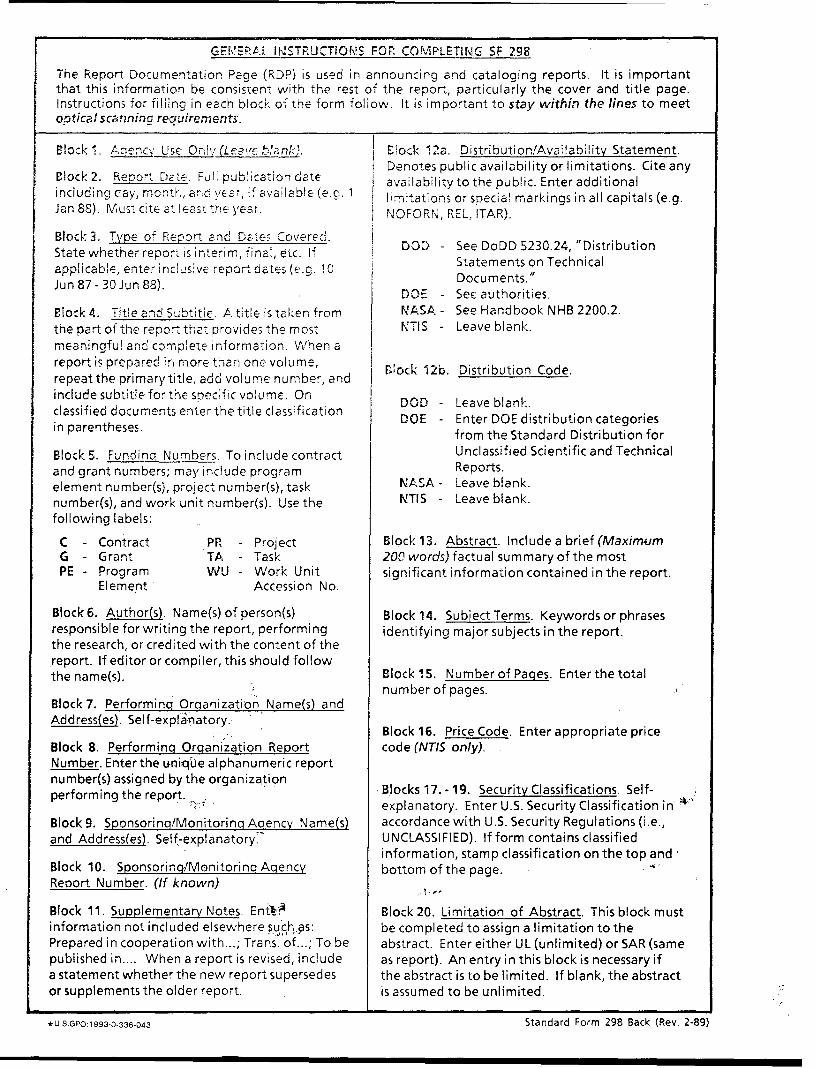
GE, ERtk.L. INSTIRUCTIONS FOR COMPLETING SF 298

The Report Documentation Page (RDP) is used in announcing and cataloging reports. It is importantthat this information be consistent with the rest of the report, particularly the cover and title page.Instructions for filling in each block of the form follow. It is important to stay within the lines to meetoptical scanning requirements.

Block 1. Apenc Use Onl, (LeavB ock 12a. Distribution/Availability Statement.Denotes public availability or limitations. Cite any

Block 2. Report Date. Full pubication date availability to the public. Enter additionalincluding day, mnonth., and yea, if available (e.g. 1i ln g a). M t a nasti year, limitations or special markings in all capitals (e.g.Jan 88). Must cite at least the year. NOFORN, REL, tTAR).

Block 3. Tpe of Repor and _D .te: Covered.Blok 3 Tve o Re'or an Daes oveed.DOD - See DoDD 5230.24, "Distribution

State whether report is interim, fine, etc. If - Seeso n TechnialStatements on Technicalapplicable, enter inclusivE report dates (e.g. 10 Documents."Jun 87 - 30 Jun 88). DOE See authorities.

Block 4. Title and Subtitie. A title is taken from NASA - See Handbook NHB 2200.2.the part of the report that provides the most NTIS - Leave blank.meaningfu! and complete information. When areport is prepared ir, more than one volume, Block 12b. Distribution Code.repeat the primary title, add volume number, andinclude subtitle for the specific volume. Onclassified documents enter the title classification DOD - Leave blank.

in parentheses. DOE - Enter DOE distribution categoriesfrom the Standard Distribution for

Block 5. Fundinq Numbers. To include contract Unclassified Scientific and Technicaland grant numbers; may include program Reports.element number(s), project number(s), task NASA - Leave blank.number(s), and work unit number(s). Use the NTIS - Leave blank.following labels:

C - Contract PR - Project Block 13. Abstract. Include a brief (Maxim-umG - Grant TA - Task 200 words) factual summary of the mostPE - Program WU - Work Unit significant information contained in the report.

Element Accession No.

Block 6. Author(s). Name(s) of person(s) Block 14. Subiect Terms. Keywords or phrasesresponsible for writing the report, performing identifying major subjects in the report.the research, or credited with the content of thereport. If editor or compiler, this should followthe name(s). Block 15. Number of Pages. Enterthe total

number of pages.Block 7. Performing Organization Name(s) andAddress(es). Self-expla-natory., Block 16. Price Code. Enter appropriate price

Block 8. Performing Organization Report code (NTIS only).Number. Enter the unique alphanumeric reportnumber(s) assigned by the organization Blocks 17.- 19. Security Classifications. Self-performing the report. .explanatory. Enter U.S. Security Classification in

Block 9. Sponsoring/Monitorina Agency Name(s) accordance with U.S. Security Regulations (i.e.,and Address(es). Self-explanatory.' UNCLASSIFIED). If form contains classified

information, stamp classification on the top andBlock 10. Sponsoring/Monitorinq Agency bottom of the page.Report Number. (If known) .,

Block 11. Supplementary Notes. Ent Block20. Limitation of Abstract. This block mustinformation not included elsewhere S'ujch,.ps: be completed to assign a limitation tothePrepared in cooperation with...; Trans. of...; To be abstract. Enter either UL (unlimited) or SAR (samepublished in.... When a report is revised, include as report). An entry in this block is necessary ifa statement whether the new report supersedes the abstract is to be limited. If blank, the abstractor supplements the older report. is assumed to be unlimited.

*U.S.GPO:1 993-0-336-043 Standard Form 298 Back (Rev. 2-89)