4D Trajectory Generation and Tracking for Waypoint-Based ... · 4D Trajectory Generation and...
15
4D Trajectory Generation and Tracking for Waypoint-Based Aerial Navigation K. BOUSSON Avionics and Control Laboratory, Department of Aerospace Sciences University of Beira Interior, 6201-001 Covilhã, PORTUGAL [email protected], [email protected] PAULO F. F. MACHADO Avionics and Control Laboratory, Department of Aerospace Sciences University of Beira Interior, 6201-001 Covilhã, PORTUGAL [email protected] Abstract: - One of the operational requirements for unmanned aerial vehicles is the autonomous navigation and control along a given sequence of waypoints, or along a predefined trajectory. Existing autonomous navigation procedures are mostly done in 3D because of the stringent certification requirements for 4D flight and due to the complexity in coping with time of arrival at waypoints, whilst actual flight plan fulfillment requires 4D navigation. The present paper deals with the 4D navigation trajectory generation and tracking of unmanned aerial vehicles along given sequences of waypoints with arrival time constraints at each of these waypoints. The approach that is used is twofold, first an optimal continuous trajectory is generated passing through the sequence of waypoints using the pseudospectral based trajectory optimization method, and then a predictive control law is used to drive the aircraft along the generated trajectory with minimum deviation. The proposed method for trajectory generation does not require slack variables to deal with the waypoints nor does it resort to the flight dynamics equations; thus the complexity of the underlying computation procedure is qualitatively lower than currently used methods. The method is successfully validated on two realistic cases giving better results than other conventional methods used in waypoint-based trajectory generation. Key-Words: - Trajectory optimization, waypoint navigation, 4D trajectory, pseudospectral approximation, predictive control. 1 Introduction The basic requirements for an aerospace vehicle are related with the capability to navigate from one point to another ensuring minimum stability and operation conditions. In this setting, trajectory optimization has always been an important research topic for aerospace navigation systems. The reasons include the necessity for generating trajectories that can take into account minimum fuel consumption, minimum arrival delay, obstacle avoidance, minimum thermal energy in case of atmospheric reentries, and other specific requirements. The common applications of trajectory optimization in aerospace navigation and robotic applications deal with minimum time problems and may be stated with state constraints. Only a handful of research activities has focused so far on the problem of waypoint-based navigation trajectory optimization. Moon and Kim [1] propose a 3D trajectory optimization method to generate a flight path going through a specified waypoint sequence. The time at which the vehicle should pass through each of these waypoints is not specified in their trajectory model; therefore, they introduce an auxiliary variable to account for the unspecified arrival times at the waypoints, which turns the overall optimization problem relatively complex. Lin and Tsai [2] present a combined mid-course and terminal guidance law design for missile interception problems. They derive analytical solutions for a closed-loop nonlinear optimal guidance law for three-dimensional mid-course and terminal guidance phases. Rao [3] improves theses analytical solutions by dealing with nonlinear terms that were neglected by Lin and Tsai. Whang and Hwang [4] propose a horizontal guidance algorithm by applying line- following to waypoint line segments sequence using linear quadratic regulator approach. In their method, the optimal waypoint changing points are computed WSEAS TRANSACTIONS on SYSTEMS and CONTROL K. Bousson, Paulo F. F. Machado E-ISSN: 2224-2856 105 Issue 3, Volume 8, July 2013
Transcript of 4D Trajectory Generation and Tracking for Waypoint-Based ... · 4D Trajectory Generation and...

4D Trajectory Generation and Tracking for Waypoint-Based Aerial Navigation
K. BOUSSON
Avionics and Control Laboratory, Department of Aerospace Sciences University of Beira Interior, 6201-001 Covilhã, PORTUGAL
[email protected], [email protected]
PAULO F. F. MACHADO Avionics and Control Laboratory, Department of Aerospace Sciences
University of Beira Interior, 6201-001 Covilhã, PORTUGAL [email protected]
Abstract: - One of the operational requirements for unmanned aerial vehicles is the autonomous navigation and control along a given sequence of waypoints, or along a predefined trajectory. Existing autonomous navigation procedures are mostly done in 3D because of the stringent certification requirements for 4D flight and due to the complexity in coping with time of arrival at waypoints, whilst actual flight plan fulfillment requires 4D navigation. The present paper deals with the 4D navigation trajectory generation and tracking of unmanned aerial vehicles along given sequences of waypoints with arrival time constraints at each of these waypoints. The approach that is used is twofold, first an optimal continuous trajectory is generated passing through the sequence of waypoints using the pseudospectral based trajectory optimization method, and then a predictive control law is used to drive the aircraft along the generated trajectory with minimum deviation. The proposed method for trajectory generation does not require slack variables to deal with the waypoints nor does it resort to the flight dynamics equations; thus the complexity of the underlying computation procedure is qualitatively lower than currently used methods. The method is successfully validated on two realistic cases giving better results than other conventional methods used in waypoint-based trajectory generation. Key-Words: - Trajectory optimization, waypoint navigation, 4D trajectory, pseudospectral approximation, predictive control. 1 Introduction The basic requirements for an aerospace vehicle are related with the capability to navigate from one point to another ensuring minimum stability and operation conditions. In this setting, trajectory optimization has always been an important research topic for aerospace navigation systems. The reasons include the necessity for generating trajectories that can take into account minimum fuel consumption, minimum arrival delay, obstacle avoidance, minimum thermal energy in case of atmospheric reentries, and other specific requirements. The common applications of trajectory optimization in aerospace navigation and robotic applications deal with minimum time problems and may be stated with state constraints. Only a handful of research activities has focused so far on the problem of waypoint-based navigation trajectory optimization. Moon and Kim [1] propose a 3D trajectory
optimization method to generate a flight path going through a specified waypoint sequence. The time at which the vehicle should pass through each of these waypoints is not specified in their trajectory model; therefore, they introduce an auxiliary variable to account for the unspecified arrival times at the waypoints, which turns the overall optimization problem relatively complex. Lin and Tsai [2] present a combined mid-course and terminal guidance law design for missile interception problems. They derive analytical solutions for a closed-loop nonlinear optimal guidance law for three-dimensional mid-course and terminal guidance phases. Rao [3] improves theses analytical solutions by dealing with nonlinear terms that were neglected by Lin and Tsai. Whang and Hwang [4] propose a horizontal guidance algorithm by applying line-following to waypoint line segments sequence using linear quadratic regulator approach. In their method, the optimal waypoint changing points are computed
WSEAS TRANSACTIONS on SYSTEMS and CONTROL K. Bousson, Paulo F. F. Machado
E-ISSN: 2224-2856 105 Issue 3, Volume 8, July 2013

through the minimization of the accelerations required for changing the waypoint line segments, and Lyapunov stability theory is used to derive a sufficient condition for the stability margin of ground speed changes. In [5], the authors present two-path planning algorithms based on Bézier curves for autonomous vehicles with waypoint and corridor constraints.
All the methods that are mentioned above deal with three-dimensional (3D) or two-dimensional (2D) waypoint-based trajectory guidance and control. Meanwhile, one of the operational requirements for unmanned aerial vehicles is the autonomous navigation and control along a given sequence of waypoints, or along a predefined trajectory. Existing autonomous navigation procedures are mostly done in 3D because of the stringent certification requirements for 4D flight, whilst actual flight plan fulfilment requires 4D navigation. Autonomous 4D navigation fulfilment will be a solution for self delivering to a time tolerance at a series of 4D waypoints, thus this will reduce uncertainty and increase predictability for both air traffic service users and providers. The present work deals with the 4D navigation trajectory generation and tracking for autonomous aerial vehicles along given sequences of waypoints, with time constraints at given check points. The difference between a 3D trajectory and a 4D trajectory is that each point of a 3D trajectory is a three-dimensional point of the physical space whereas each point of a 4D trajectory is composed of a three-dimensional point and the time at which the vehicle is scheduled to pass at that point. Although the 4D trajectory concept has been used in the flight planning for commercial aircraft missions, there has been so far no systematic method for designing such trajectories from computational standpoint.
Trajectory generation problems can be solved by optimal control techniques. There are two approaches to solve optimal control problems: the direct approach and the indirect one [6]. The indirect methods are based on Pontryagin maximum principle that enables to transform an optimal control problem into Euler-Lagrange equations. On the other hand, the direct approach is based on the transformation of optimal control problems into nonlinear programming problems. In the current work, we address the direct methods to solve 4D trajectory generation problems.
To transform an optimal control problem into a nonlinear programming problem it is necessary to parameterize the state and the control vectors that are involved [7]. Convergence rate to the actual
solution and the corresponding accuracy depend mostly on the parameterization method rather than on the optimization algorithm that is used to solve the problem. The present paper describes a trajectory generation method based on Chebyshev pseudo-spectral approximation [8-11] that has been developed for the direct approach to determine the optimal control trajectories of higher-order nonlinear dynamic system. That procedure is based on the approximation of both controls and states by interpolating polynomials at the Chebyshev nodes. The interest of the Chebyshev pseudo-spectral methods over former ones using Runge-Kutta scheme [12] or collocation methods [13] is that the best polynomial approximation in the sense of Chebyshev norm and the derivatives of the approximating polynomials are exactly known, whilst the other approaches resort to derivative approximations.
The paper is organized as follows: section 2 states the problem to be solved herein; then the methods of pseudospectral parameterization for optimal control together with a predictive control method for the optimal trajectory following are presented in section 3, and section 4 demonstrates the suitability of the proposed method on realistic optimal navigation along 4D waypoint-based trajectory problems for unmanned aerial vehicles. The numerical results of these application examples clearly show that the proposed parameterization scheme provides effective means for accurate generation and tracking control of 4D trajectories. Section 5 concludes the paper. 2 Problem Statement The main goal of navigation guidance is to provide a reference velocity refV , path angle refγ and heading refψ to enable the aircraft go through a predefined sequence of waypoints 0 1, ,..., MP P P .
Most of the approaches consider the waypoints defined by tridimensional coordinate positions
( , , ),k k k kP hλ ϕ= 0,1,..., ,k M= and do not take into account the time. The idea of the present paper is to redefine that concept by including the arrival time restriction to the description of 4D waypoints defined as: ( , , , ),k k k k kP hλ ϕ τ= 0,1,...,k M= , where
kτ is the arrival time at the corresponding waypoint. The problem to be solved is to control the
aircraft to navigate along a specified sequence of 4D waypoints, ( , , , ),k k k k kP hλ ϕ τ= 0,1,..., ,k M= from the initial waypoint 0( )P to the last ( )MP while minimizing the arrival delay at each waypoint kP .
WSEAS TRANSACTIONS on SYSTEMS and CONTROL K. Bousson, Paulo F. F. Machado
E-ISSN: 2224-2856 106 Issue 3, Volume 8, July 2013

We propose in the following section a method that will determine the optimal control and state trajectory along specified waypoints based on the pseudospectral trajectory optimization approach, and a predictive control method that will enable the vehicle to track the optimal state trajectory. 3 Proposed Method Optimal control of a dynamical system consists in finding a control vector function : ( )u t u t that minimizes a cost functional defined as:
0
( , , ) ( , ( ), ( ), )
( , ( ), ( ), )f
f f fJ x u x u
L x u dτ
τ
η τ τ τ η
τ τ τ η τ
= Φ
+ ∫ (1)
where Φ and L are functionals, nx ℜ∈ is the state vector, mu ℜ∈ the control vector, sη∈ℜ the parameter vector, andτ the time ( 0τ and fτ being respectively the initial and final time-instants), subject to the following constraints on the dynamics of the system:
0
min max
( , , , )
f
x f x uτ ητ τ τ
η η η
=≤ ≤
≤ ≤
(2)
The optimal control problem may also be subject
to equality and inequality constraints on the state and the control, as described respectively by:
( , , , ) 0h x uτ η = (3) ( , , , ) 0g x uτ η ≤ (4)
The problem may also be subject to boundary
(initial and terminal) conditions as well and described as:
0( ( ), ( )) 0fx xτ τΨ = (5)
3.1 Pseudospectral Parameterization The pseudospectral methods have been developed for the direct approach in optimal control [8-11]. The main goal is to find the optimal trajectories of the nonlinear systems of high order. Lagrange and Chebyshev polynomials are used in these methods to approximate the state and control variables. The procedure for approximating these variables is based
on Legendre polynomials built on Chebyshev nodes kt that are described as cos( ),kt k Nπ=
0,1,...,k N= , where N is a given integer number greater than or equal to one ( 1)N ≥ . These nodes kt lie in interval [ 1,1]− and are the extrema of the Nth-order Chebyshev polynomial
( )NT t , knowing that a Chebyshev polynomial of jth-order is defined in trigonometric form as:
( ) cos( arccos( ))
0,1,...,jT t j t
j N=
= (6)
where ‘arccos’ is the arc cosine function. It can be easily checked that ( ) cos( )j kT t jk Nπ= for any
0,1,...,j N= , and any Chebyshev node kt , 0,1,...,k N= .
Consider a set of N+1 Chebyshev nodes kt in interval [ 1,1]− ; then, the Lagrange interpolating polynomials of order N are defined for as:
1 2
2
0
( 1) (1 ) ( )( )( )
2 ( ) ( )
kN
kk k
Nl k l
lk l
t T ttc N t t
T t T tNc c
ϕ+
=
− −=
−
= ∑
(7)
,...,,1,0 Nk = with:
0 21, 1,..., 1
N
k
c cc k N= == = −
(8)
It can be noticed that each Lagrange polynomial is such that:
1( )
0k l kl
if k lt
if k lϕ δ
== = ≠
(9)
Because the problem of the optimal control is
formulated on the time interval 0, fτ τ and the Chebyshev nodes are defined on the interval [ ]1,1− , it is necessary to resort to the following transformation to redefine the optimal control problem with the new time variable t in interval [ ]1,1− as:
WSEAS TRANSACTIONS on SYSTEMS and CONTROL K. Bousson, Paulo F. F. Machado
E-ISSN: 2224-2856 107 Issue 3, Volume 8, July 2013

0
0
2 f
f
tτ τ ττ τ− −
=−
(10)
where the actual time τ is obtained conversely as
0 0(( ) ( )) 2f ftτ τ τ τ τ= − + + . For (N+1) Chebyshev nodes, the time-based parameterizations ( )Nx t of the state vector and
( )Nu t of the control vector are defined respectively (on the basis of the new time variable t) as:
0
( ) ( )N
Nk k
kx t x tϕ
=
= ∑ (11)
0
( ) ( )N
Nk k
ku t u tϕ
=
= ∑ (12)
where each kϕ is the Lagrange polynomial as
defined above, and vectors nkx ∈ℜ and m
ku ∈ℜ are respectively the values of the state and control vectors at Chebyshev nodes kt : ( ), ( )k k k kx x t u u t≡ ≡ (13) With the parameterization above, the derivative of the state vector at each Chebyshev node kt is approximated as:
0 0
( ) ( )N N
Nk l l k kl l
l lx t x t d xϕ
= =
= =∑ ∑ (14)
Where the elements kjd of the differentiation matrix
,( )kl k lD d= are defined as:
2
2
2
( 1) ,( )
2 1, 06
2 1,6
, 1 12(1 )
k lk
l k l
kl
l
l
c k lc t t
N k ld
N k l N
t k l Nt
+ −≠ −
+= ==
+− = =− ≤ = ≤ − −
From equation (13), for each 1,...,k N= , let ,kjx ( 1,..., ),j n= be the elements of the state vector
kx , and ,klu ( 1,..., ),l m= be the elements of the control vector ku . Similarly, let the elements of the
parameter vector sη∈ℜ be defined as 1... sη η . Finally, consider the following vector composed of all the unknowns of the optimal control problem:
[ ]01 01 02 02 1... ...Nn Nm sy x u x u x u η η= (15) Then, from equations (10-14), the optimal control problem can be formulated as:
0
0
0
min max
Min ( )
subect to:
( , , , )2
( , , , ) 0( , , , ) 0, 0,1,...,( ( ), ( )) 0
y
Nf
kl l k k kl
k k k
k k k
f
J y
d x f t x u
h t x ug t x u k N
x x
τ τη
ηη
τ τ
η η η
=
− =
=≤ =
Ψ =
≤ ≤
∑ (16)
3.2 Modeling 4D Navigation Problem
In the present section, the modeling of the four-dimensional navigation problem is described as an optimal control problem.
3.2.1 Problem Formulation Let us consider an aircraft that is supposed to navigate along a sequence of ( 1)M + waypoints kP , ( 0,1,...,k M= ). Assume each of these waypoints to be described as a four-dimensional state vector:
Tkkkkk hP )( τϕλ= (17)
where: kλ is the longitude of the waypoint ( kP ), kϕ the latitude, kh the altitude (with respect to Sea level), and kτ the time the aircraft is scheduled to arrive at waypoint kP . The problem to be solved is to generate a flight trajectory going from the initial waypoint ( 0P ) to the terminal waypoint ( f MP P≡ ) passing through the sequence of the specified waypoints. Therefore, the cost functional associated with the problem stated above may be defined as: ( ) ( ( )) ( ( ))T
f f f f fJ u P s Q P sτ τ= − − (18)
WSEAS TRANSACTIONS on SYSTEMS and CONTROL K. Bousson, Paulo F. F. Machado
E-ISSN: 2224-2856 108 Issue 3, Volume 8, July 2013

where ( )fs τ is the terminal position of the aircraft (at time f Mτ τ≡ ), fQ a positive definite matrix of appropriate dimension, and u the control vector of the navigation model that is described in the following section .
3.2.2 Navigation Model The following differential equations model the dynamics of the navigation process:
cos sin( )cose
VR h
γ ψλϕ
=+
(19)
cos cos
e
VR hγ ψϕ =+
(20)
sinh V γ= (21) 1V u= (22) 2uγ = (23) 3uψ = (24) where: λ is the longitude of the location of the aircraft, ϕ the latitude, h the altitude (with respect to Sea level), V the speed of the aircraft, γ its flight path angle, and ψ its heading (with respect to the geographical North). The variables 1 2,u u and 3u are respectively the acceleration, the flight path angle rate and the heading rate. The state and control vectors of the above model are described respectively as:
( )Tx h Vλ ϕ γ ψ= (25) 1 2 3( )Tu u u u= (26)
3.2.3 Navigation Constraints Due to aerodynamic and structural limits, bound constraints are imposed on the state and control vectors and described as: min max , 1,2,3i i iu u u i≤ ≤ = (27) min maxV V V≤ ≤ (28) min maxγ γ γ≤ ≤ (29) The naive way to fly from waypoint to waypoint is to strictly pass through each waypoint kP exactly at the specified time kτ . Meanwhile, in practice, this may not be possible due to disturbances that may give rise to navigation inaccuracies, or even inappropriate due to the topology of the waypoint locations that may force the aircraft to take a too
steep path curvature when switching from a waypoint to the next. Therefore, an appropriate way is rather to impose the following navigation constraint at each waypoint:
2( ) , ( 1,..., )k kP s k Mτ σ− ≤ = (30)
where ( )ks τ is the position of the aircraft at time kτ ,
0σ > and 2
. is the Euclidean norm. Constraint (30) expresses that the aircraft shall be at time kτ at a distance less than σ from waypoint kP , which constrains the aircraft to merely be, at time kτ , in a sphere of radius σ and centred at waypoint
kP (instead of strictly be at kP at time kτ ).
3.3 Computing the Optimal Navigation Trajectory The 4D trajectory generation problem has been modeled above as a trajectory optimization problem. Therefore, the pseudospectral method described in section 3.1 may be used to find the optimal trajectory for navigation along a given sequence of waypoints. A numerical simulation of an actual case will be presented in section 4.
3.4 Trajectory Control Once the optimal state trajectory is found, as was the purpose of the above sections, it is necessary to design a flight control strategy to enable the aircraft to track that optimal trajectory based on the navigation equations and the flight dynamics model of the aircraft. There exist many control methods that may be used to track the optimal trajectory resulting from the method described in above sections; some of these methods are general ones [14-19] and others are specific to flight control [20,21]. Meanwhile, the trajectory tracking procedure that is used in the present paper relies on designing a specific and more suitable nonlinear control law based on predictive control methods [14-17].
3.4.1 One-Step Predictive Control
Let the following be the model of a dynamic system viewed as a combination of two subsystems: 1 1( )x f x= (31) 2 ( , )x g x u= (32)
WSEAS TRANSACTIONS on SYSTEMS and CONTROL K. Bousson, Paulo F. F. Machado
E-ISSN: 2224-2856 109 Issue 3, Volume 8, July 2013

where 11
nx R∈ is the state vector of the first subsystem, 2
2nx R∈ the state vector of the second
subsystem, 1 2( )T T T nx x x R= ∈ the state vector of the overall system, with 1 2n n n= + the total dimension of the state space; and mu U R∈ ⊂ the control vector, where U is a compact domain of feasible controls. Equation (32) may be approximated about a given control vector lu as: 2 ( , ) ( )lx g x u B x u= + (33)
With lu u u= − , and:
( , )( )lu u
g x uB xu =
∂ = ∂
For any 0,k fτ τ τ ∈ , let define ( )k kx x τ= ,
1 1( )k kx x τ= , 2 2 ( )k kx x τ= , ( )k ku u τ= , and
2 ( ) ( , )lf x g x u≡ . Assuming the relative degree of equation (31) and that of equation (33) to be one and zero respectively with respect to the control vector (as is the case for the flight dynamics model in section 3.4.2.), equation (31) can be approximated using a second order Taylor series expansion so as to make the control vector ku appear in the expression of 1 1kx + , and equation (33) can be approximated as well using a first order Taylor series expansion. It comes:
1 1 1 12
1 1 2 2
. ( )
(( ) 2)[ ( ) ( ( ) ( ) )]k k k
k k k k
x x f xF f x F f x B x u
τ
τ+ = + ∆
+ ∆ + + (34)
2 1 2 2.( ( ) ( ) )k k k k kx x f x B x uτ+ = + ∆ + (35)
where:
11
1
( )
kx x
f xFx
=
∂= ∂
22
2
( )
kx x
f xFx
=
∂= ∂
Let refx1 and refx2 be the reference trajectories of state vectors 1x and 2x respectively, and the tracking error of these reference trajectories be defined as:
1 1 1 1 1 1
2 1 2 1 2 1
refk k k
refk k k
e x xe x x
+ + +
+ + +
= −
= − (36)
Then the objective function to be minimized so as to find the control that enables us to track the reference state trajectory is given as:
1 1 1 1 1 2 1 2 2 11 1( )2 2
T Tk k k kJ u e Q e e Q e+ + + += + (37)
Where 1Q and 2Q are positive definite matrices. This minimization problem may be subject to constraints on the stepsize h, and on the control and state vectors in the form: min max0 h h h< ≤ ≤ 1( ) 0c u ≤ (38) 2 1 2( , ) 0c x x ≤ where 1(.)c and 2 (.)c are appropriate functions.
3.4.2 Aircraft Flight Dynamics Model Before we apply the proposed Predictive Control method above to 4D flight trajectory tracking, it is necessary to describe the dynamic model. The aircraft dynamic model is described by the following equations [22]:
max cos( ) sinT TT DV gm
δ α ε γ+ −= − (39)
max sin( ) cos cosT TL T gmV V
δ α εγ φ γ+ += − (40)
max sin( ) sincos
T TL TmV
δ α εψ φγ
+ += (41)
( sin cos ) tanp q rφ φ φ θ= + + (42) cos sinq rθ φ φ= − (43)
θ α γ= + (44)
2
1 ( ( ( ) )
( ( ) ))
z l y zx z xz
xz n x y z xz
p I QSbC I I qrI I I
I QSbC I I I pq I qr
= + − +−
+ − + −
(45)
2 21 ( ) ( )m xz z xy
q QScC I r p I I rpI = + − + − (46)
2
1 ( ( ( ) )
( ( ) ))
x n x yx z xz
xz l y x z xz
r I QSbC I I pqI I I
I QSbC I I I qr I pq
= + − +−
+ − − +
(47)
WSEAS TRANSACTIONS on SYSTEMS and CONTROL K. Bousson, Paulo F. F. Machado
E-ISSN: 2224-2856 110 Issue 3, Volume 8, July 2013

where V is the aircraft velocity, γ is the flight path angle, φ is the bank angle, θ the pitch angle, p, q, r are the roll, pitch and yaw rates respectively; α is the angle of attack, Tε is the angle between the thrust vector and the longitudinal axis of the aircraft, , ,x y z xzI I I I are the moments of inertia, L the lift force, D the drag force, maxT the maximum thrust available, Q the dynamic pressure, S the wing reference area, b the wing span, c the mean chord,
,l qC C , and nC are the roll, pitch and yaw moment coefficients.
Before applying the predictive control method to this system, it is necessary to split the flight dynamic model above into two interlinked subsystems so as to deal with a cascade system. The two subsystems are defined as follows:
The first subsystem is composed of the following state and control vectors in accordance with the template model described in equations (31,32):
1 ( )Tx hλ ϕ= (48)
2 ( )Tx V γ ψ= (49) ( )T
e Tu θ φ δ δ= (50) where eδ (elevator deflection) and Tδ (throttle) are the primary controls, and θ and φ the secondary controls. The reference vector 1
refx is defined by the reference navigation path, and 2
refx by the velocity, flight path angle and heading angle that are necessary to track 1
refx . The second subsystem is described by the
following state and control vectors:
1 ( )Tx θ φ= (51)
2 ( )Tx p q r= (52) ( )T
a ru δ δ= (53)
Where aδ is the aileron deflection and rδ the rudder deflection. The reference vector 1
refx is defined as
1 ( )ref ref ref Tx θ φ= , and 2 (0 0 0)ref Tx = to ascertain stepwise quasi-equilibrium conditions while tracking 1
refx .
4. Simulations In this section are presented two applications, the first is a typical commercial flight and the second
mission is a flight in circuit. In both applications the air vehicle used is the UAV SkyGu@rdian constructed in University of Beira Interior. In both situations were applied the Pseudospectral method and a Collocation method with trapezoidal integration scheme, and only for the second example is applied the control method because it is worst case. For the solution search of the problem, it was used the fmincon function of optimization toolbox of MatLab for solve the nonlinear programming problem. The computer used for test and simulation was an Acer Aspire 1690 with 2.0 GHz CPU and 1GB of RAM.
4.1. Example 1 The first example is a straight flight typically of civil flights. Table 1 shows the waypoints list. Each waypoint is defined in geodetic coordinates ( , , )hλ ϕ and must be specified the desired time (τ) to reach it. In this specific mission, both methods of parameterization achieve a solution for the problem, the final values of position as well as the cost function are represented in Table 2.
When applied the Collocation technique, we consider the nodes coincident with the waypoints, this is valid because the time was expressed in hours and the difference between waypoints is small that allows an acceptable step of integration. We tried some distributions of collocation nodes but finally we found that satisfactory results could only be achieved with sufficiently high number of nodes.
As in Pseudospectral method the nodes are specified on Chebyshev nodes in [-1, 1] interval, the problem with node placement does not arise. We considered 20 nodes for this example because the method converged accurately using this number of nodes, given practically the same result as when higher numbers of nodes are used.
Table 1. List of waypoints for the straight mission N λ ϕ h τ [deg min sec] [deg min sec] [m] [hour] 1 7º 29’ 35.00” W 39º 49’ 25.71” N 400 0.000 2 7º 29’ 37.00” W 39º 50’ 34.82” N 500 0.035 3 7º 29’ 39.00” W 39º 51’ 33.38” N 600 0.070 4 7º29’ 41.00” W 39º 52’ 39.86” N 600 0.080 5 7º29’ 41.50” W 39º 54’ 50.26” N 700 0.120 6 7º29’ 42.00” W 39º 56’ 55.38” N 800 0.165 7 7º 29’ 45.00” W 39º 59’ 15.04” N 800 0.210 8 7º 29’ 47.00” W 40º 01’ 17.12” N 800 0.245 9 7º 29’ 49.00” W 40º 03’ 45.92” N 800 0.280 10 7º 29’ 51.00” W 40º 05’ 31.38” N 800 0.325 11 7º 29’ 53.00” W 40º 08’ 12.56” N 800 0.370 12 7º 29’ 55.00” W 40º 11’ 06.43” N 750 0.415 13 7º 30’ 00.00” W 40º 14’ 07.43” N 650 0.450 14 7º 30’ 02.00” W 40º 17’ 02.02” N 600 0.480
WSEAS TRANSACTIONS on SYSTEMS and CONTROL K. Bousson, Paulo F. F. Machado
E-ISSN: 2224-2856 111 Issue 3, Volume 8, July 2013

Table 2: Results of final values in straight mission ( )
[ ]f
radλ τ ( )
[ ]f
radϕ τ
( )[ ]
fhKmτ
J
Collocation -0.1309
0.7031
0.5998
82.8 10−× Pseudospectral -0.1309
0.6999
0.5058
43.7 10−×
It is possible to see in Figure 1 the trajectories found by both methods representing the longitude, latitude and altitude respectively. The Figures 3, 4 and 5 represent the velocity, path angle and heading respectively, and figures 6, 7 and 8 represent the controls. In Figure 2 is represented the trajectory in 3 dimensions.
The velocity in Figure 3 shows a constant behavior because the arrival times at each waypoint were defined as such, the control u1, that is, the variation of velocity, is the depicted in Figure 6, which is practically identical in both methods. The path angle Figure 4 generated by pseudospectral method is slightly smoother than the path angle generated by collocation method, but the differences can be seen well in Figure 7 that represents the variation of the path angle (u2), here the pseudospectral method shows a trajectory with more smoothness than the collocation method. The heading trajectory, Figure 5, and control u3 in Figure 8 representing the variation of heading do not present significantly differences between the two methods.
This result shows that the pseudospectral method achieves a final solution almost equal to the collocation method but with the controls trajectories are smoother, which allows improving cost of the mission.
Figure 1: (a) Longitude, (b) Latitude and (c) Height vs. Time for Example 1
WSEAS TRANSACTIONS on SYSTEMS and CONTROL K. Bousson, Paulo F. F. Machado
E-ISSN: 2224-2856 112 Issue 3, Volume 8, July 2013

Figure 2: 3D Trajectory for Example 1
Figure 3: Velocity vs. Time for Example 1
Figure 4: Path Angle vs. Time for Example 1
Figure 5: Heading vs. Time for Example 1
Figure 6: Control u1 vs. Time for Example 1
Figure 7: Control u2 vs. Time for Example 1
WSEAS TRANSACTIONS on SYSTEMS and CONTROL K. Bousson, Paulo F. F. Machado
E-ISSN: 2224-2856 113 Issue 3, Volume 8, July 2013
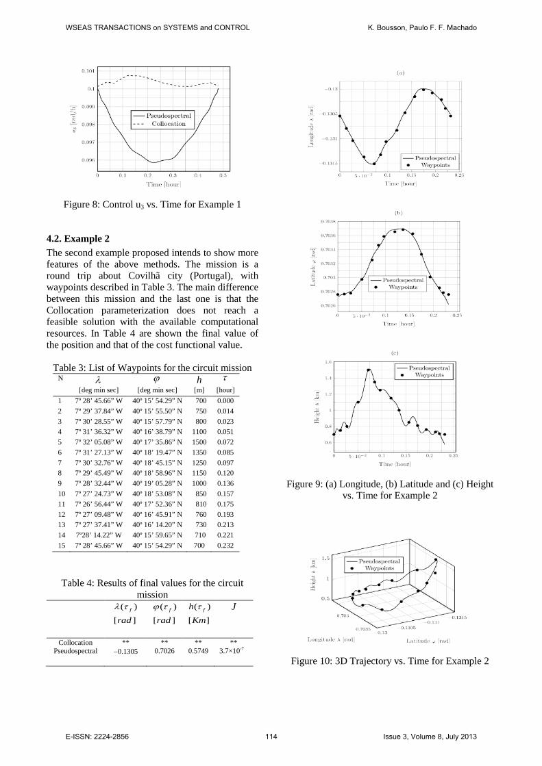
Figure 8: Control u3 vs. Time for Example 1
4.2. Example 2 The second example proposed intends to show more features of the above methods. The mission is a round trip about Covilhã city (Portugal), with waypoints described in Table 3. The main difference between this mission and the last one is that the Collocation parameterization does not reach a feasible solution with the available computational resources. In Table 4 are shown the final value of the position and that of the cost functional value.
Table 3: List of Waypoints for the circuit mission N λ ϕ h τ
[deg min sec] [deg min sec] [m] [hour] 1 7º 28’ 45.66” W 40º 15’ 54.29” N 700 0.000 2 7º 29’ 37.84” W 40º 15’ 55.50” N 750 0.014 3 7º 30’ 28.55” W 40º 15’ 57.79” N 800 0.023 4 7º 31’ 36.32” W 40º 16’ 38.79” N 1100 0.051 5 7º 32’ 05.08” W 40º 17’ 35.86” N 1500 0.072 6 7º 31’ 27.13” W 40º 18’ 19.47” N 1350 0.085 7 7º 30’ 32.76” W 40º 18’ 45.15” N 1250 0.097 8 7º 29’ 45.49” W 40º 18’ 58.96” N 1150 0.120 9 7º 28’ 32.44” W 40º 19’ 05.28” N 1000 0.136 10 7º 27’ 24.73” W 40º 18’ 53.08” N 850 0.157 11 7º 26’ 56.44” W 40º 17’ 52.36” N 810 0.175 12 7º 27’ 09.48” W 40º 16’ 45.91” N 760 0.193 13 7º 27’ 37.41” W 40º 16’ 14.20” N 730 0.213 14 7º28’ 14.22” W 40º 15’ 59.65” N 710 0.221 15 7º 28’ 45.66” W 40º 15’ 54.29” N 700 0.232
Table 4: Results of final values for the circuit mission
( )[ ]
f
radλ τ ( )
[ ]f
radϕ τ
( )[ ]
fhKmτ
J
Collocation ** ** ** ** Pseudospectral −0.1305 0.7026 0.5749 3.7×10⁻⁷
Figure 9: (a) Longitude, (b) Latitude and (c) Height vs. Time for Example 2
Figure 10: 3D Trajectory vs. Time for Example 2
WSEAS TRANSACTIONS on SYSTEMS and CONTROL K. Bousson, Paulo F. F. Machado
E-ISSN: 2224-2856 114 Issue 3, Volume 8, July 2013

For Collocation method we tried several sets of nodes, but none of these attempts achieved a feasible solution. On the other hand the pseudospectral method reached an acceptable solution. We used 25 nodes because the method converged for this number of nodes. For more than 25 nodes, the computation became very heavy in the framework of Matlab capabilities. Figure 9, representing longitude, latitude and altitude respectively. The Figures 11, 12 and 13 represent velocity, path angle and heading respectively, and Figures 14, 15 and 16 represent the controls. The Figure 10 represents the trajectory in three dimensions. Although the cost functional, for this example, presents a low value it is not sufficient for trajectory overlap with the final waypoint, this is visible in Figure 9(c) and happens because the optimization software cannot refine the solution. The velocity Figure 11 and velocity variation Figure 14 have an almost constant behavior, this fact was expected because, similarly to example I, the time arrival in waypoints was specified with this intention. Path angle Figure 12 and path angle variation Figure 15 show a behavior more oscillatory than the other variables. The increase of nodes solve this problem, nevertheless the path angle shall not exceed the aerodynamics limits of aircraft. Finally the heading in Figure 13 and its variation, Figure 16, show a behavior in accordance with the track. Also as in the first example, the pseudospectral methods give us a smoother trajectory, and with a better optimization tool than was used, the trajectory can be improved.
Figure 11: Velocity vs. Time for Example 2
Figure 12: Path Angle vs. Time for Example 2
Figure 13: Heading vs. Time for Example 2
Figure 14: Control u1 vs. Time for Example 2
Figure 15: Control u2 vs. Time for Example 2
WSEAS TRANSACTIONS on SYSTEMS and CONTROL K. Bousson, Paulo F. F. Machado
E-ISSN: 2224-2856 115 Issue 3, Volume 8, July 2013

Figure 16: Control u3 vs. Time for Example 2 Table 5: RMSE between the reference trajectory and
control output s V γ ψ
[km] [m/s] [rad] [rad] 0.2310 2.0523 0.0041 0.0003
The next step is to apply the predictive control technique. In this example only was applied the control method to a portion of trajectory because the optimization toolbox used in this work not was able to find the whole control trajectory in acceptable time. Due to this the predictive control was applied to three first waypoints.
In Table 5 is show the RMSE (Root Mean Square Error), calculated by:
0
1 22
0
1 ( ) ( )f
ref
f
RMSE s s dtτ
τ
τ ττ τ
= − −
∫ (54)
The Figure 17 represents the position behavior of the UAV. The control it seems ensures the fulfillment of the mission, although the accuracy is not the better. Figures 18, 19 and 20 show the behavior of the guidance variables, the oscillation that happens in these variables is due to the use of the mean maximum Traction in the dynamic model and the control method have difficulty in fulfill the time restriction imposed by the reference trajectory, but the peak to peak oscillation is within the acceptable values for that UAV. The Figures 21 and 22 are a consequent response of the position and guidance variables.
Figure 17: (a) Longitude, (b) Latitude and (c) Height vs. Time for Example 2 - Control
Demonstration
WSEAS TRANSACTIONS on SYSTEMS and CONTROL K. Bousson, Paulo F. F. Machado
E-ISSN: 2224-2856 116 Issue 3, Volume 8, July 2013

Figure 18: Velocity vs. Time for Example 2 - Control Demonstration
Figure 19: Path Angle vs. Time for Example 2 - Control Demonstration
Figure 20: Heading vs. Time for Example 2 - Control Demonstration
Figure 21: Bank Angle vs. Time for Example 2 - Control Demonstration
Figure 22: Pitch vs. Time for Example 2 - Control Demonstration
5. Conclusion This paper described a method for designing a 4D optimal navigation trajectories and a flight control strategy to track these optimal trajectories during unmanned missions. The 4D trajectories have the expected time of arrival at each waypoint in addition to the desired position. The pseudospectral approach was used for the parameterization of optimal trajectories built on Chebyshev nodes. Two examples were presented in which the pseudoespectral method was compared with the collocation method with trapezoidal integration scheme. The pseudospectral method achieved appropriate solutions for the presented applications whereas the collocation method was able to solve only one of the applications. Although the pseudospectral method found solutions for the two applications, what is relevant is that the control
WSEAS TRANSACTIONS on SYSTEMS and CONTROL K. Bousson, Paulo F. F. Machado
E-ISSN: 2224-2856 117 Issue 3, Volume 8, July 2013

trajectories were smoother than in the case of the collocation method. A one-step ahead predictive control method was presented and used for controlling the aircraft along the trajectories that were generated. This method intends to be simple and robust, and it lends itself to real time control. However, although the results that were obtained in these case studies were interesting and promising, more research work will be needed for the controller to enable the aircraft track predefined optimal trajectories in actual unmanned missions in which fuel saving and other operational requirements are central to the mission concerns. Acknowledgment This research was conducted in the Aeronautics and Astronautics Research Group (AeroG) of the Associated Laboratory for Energy, Transports and Aeronautics (LAETA), and supported by the Portuguese Foundation for Sciences and Technology (FCT). References: [1] G. Moon and Y. Kim, Flight Path Optimization
Passing Through Waypoints for Autonomous Flight Control Systems, Engineering Optimization, Vol. 37, No. 7, October 2005, pp. 755–774.
[2] C. F. Lin and L. L. Tsai, Analytical Solution to Optimal Trajectory Shaping Guidance, Journal of Guidance, Control and Dynamics, Vol. 10, No. 1, 1987, pp. 61-66. M. N.
[3] M.N. Rao, Analytical Solution to Optimal Trajectory Shaping Guidance, Journal of Guidance, Control and Dynamics, Vol. 12, No. 4, 1989, pp. 600-601.
[4] I. H. Whang and T. W. Hwang, Horizontal Waypoint Guidance Design Using Optimal Control, IEEE Transactions on Aerospace and Electronic Systems, Vol. 38, No. 3, 2002, pp. 1116-1120.
[5] J. W. Choi, R. E. Curry and G. H. Elkaim, Continuous Curvature Path Generation Based on Bézier Curves for Autonomous Vehicles, IAENG International Journal of Applied Mathematics, Vol. 40, No. 2, 2010, Paper Nº IJAM 40-2-07.
[6] J. T. Betts, Survey of Numerical Methods for Trajectory Optimization, Journal of Guidance, Control, and Dynamics, Vol. 21, No. 2, March-April 1998, pp. 193–207.
[7] D. G. Hull, Conversion of Optimal Control Problems into Parameter Optimization Problems, Journal of Guidance, Control, and
Dynamics, Vol. 20, No. 1, January-February 1997, pp. 57–60.
[8] J. Elnagar, The Pseudospectral Legendre Method for Discretizing Optimal Control Problems, IEEE Transactions on Automatic Control, Vol. 40, No. 10, 1995, pp. 1793-1796.
[9] F. Fahroo, and I. M. Ross, Direct Trajectory Optimization by a Chebyshev Pseudospectral Method, Journal of Guidance, Control and Dynamics, Vol. 25, No. 1, 2002, pp. 160-166.
[10] L. R. Lewis, I. M. Ross, and Q. Gong, Pseudospectral Motion Planning Techniques for Autonomous Obstacle Avoidance, Proceedings of the 46th IEEE Conference on Decision and Control, Vol. 3, New Orleans, 2007, pp. 2210–2215.
[11] K. Bousson, Chebychev Pseudospectral Trajectory Optimization of Differential Inclusion Models, SAE World Aviation Congress, 2003 Aerospace Congress and Exhibition, Montreal, Canada, September 2003, Paper 2003–01–3044.
[12] A. Schwartz, and E. Polak, Consistent Approximations for Optimal Control Problems Based on Runge-Kutta Integration, SIAM Journal on Control and optimization, Vol. 34, No. 4, 1996, pp. 1235-1269.
[13] C. R. Hargraves, and S.W. Paris, Direct Trajectory Optimization Using Nonlinear Programming and Collocation, Journal of Guidance, Control and Dynamics, Vol. 10, No. 4, 1987, pp. 338-342.
[14] P. Lu, Optimal Predictive Control of Continuous Nonlinear Systems, International Journal of Control, Vol. 62, No. 3, 1995, 633-649.
[15] D. Q. Mayne, and H. Michalska, Receding Horizon Control of Nonlinear Systems. IEEE Transaction on Automatic Control, 35, 1990, pp. 814-824.
[16] D. Q. Mayne, J. B. Rawlings, C. V. Rao and P. O. M. Scokaert, Constrained Model Predictive Control: Stability and Optimality. Automatica, 36, 2000, pp. 789–814.
[17] H. Michalska and D. Q. Mayne, Robust Receding Horizon Control of Constrained Nonlinear Systems. IEEE Transaction on Automatic Control, 38, 1993, pp. 1623-1633.
[18] M.M. Belhaouane, R. Mtar, H.B. Ayadi, and N.B. Braiek, An LMI Technique for the Global Stabilization of Nonlinear Polynomial Systems, International Journal of Computers, Communications, & Control, Vol.4, No. 4, 2009, pp. 335-348.
WSEAS TRANSACTIONS on SYSTEMS and CONTROL K. Bousson, Paulo F. F. Machado
E-ISSN: 2224-2856 118 Issue 3, Volume 8, July 2013

[19] R.E. Precup, M.L. Tomescu, and St. Preitl, Fuzzy Logic Control System Stability Analysis Based on Lyapunov’s Direct Method, International Journal of Computers, Communications & Control, Vol. 4, No. 4, 2009, pp. 415-426.
[20] T.-V. Chelaru, and V. Pana, Stability and Control of the UAV Formation Flight, WSEAS Transactions on Systems and Control, Vol. 5, No. 1, 2010, pp. 26-36.
[21] E. Kyak, and F. Caliskan, Design of Fault Tolerant Flight Control System, WSEAS Transactions on Systems and Control, Vol. 5, No. 6, 2010, pp. 454-463.
[22] B. Etkin, and L.D. Reid, Dynamics of Flight: Stability and Control, 3rd edition, Wiley, 1995.
WSEAS TRANSACTIONS on SYSTEMS and CONTROL K. Bousson, Paulo F. F. Machado
E-ISSN: 2224-2856 119 Issue 3, Volume 8, July 2013