4.1 Extending the Walker code - Virginia Tech

Chapter 4 An extension of the Walker code and application.

39

4.1 Extending the Walker code

Changing the code so that the second boundary condition is that of a specified temperature on the

back face of a slab, we were able to move away from the semi-infinite solid limitation. The heat

fluxes at the back face and the surface are obviously dependent on the temperature gradient at

that position, which in turn is dependent on the measured temperature there. The boundary

condition at the thermocouple at the back is given below. “back” is the temperature at the back

face at a specific point in time. “for” is twice the Fourier number, αt/L2. a, b, c, and d are the

coefficients of the tridiagonal matrix, used to solve for the temperature distribution through the

solid at a given point in time. It is important to note that the changes were made to the

conduction solver and not to the inverse method itself.

C Interior boundary at a specific temperature a(nx) = - 0.5 * for b(nx) = 1 + for c(nx) = 0 r(nx) = (0.5*for*back) + t(nx-1) The use of this boundary condition ensures that the slope of the temperature curve is not zero at

the back, as is the case with the semi-infinite approach [11]. To be able to do this, all the

subroutines need to have an extra variable, which is the temperature at the back face. The

penetration depth was also set at 0.025m, for this specific blade in the cascade tunnel. The user

can change this value at any time to any value. These tests will be described below. This value

can easily be changed for different situations. The output of this program is given in five

columns. These are the time, the guessed flux, the surface temperature, the temperature at the

back and then the heat flux at the surface. Other changes were made to save the values of the

temperatures at the back and the subroutines were changed in such a way that the back face

temperature was incorporated there as well. For example:

ct = 1 32 READ(10,*,END=31) tm(ct), q0(ct), y(ct), bft(ct) ct = ct + 1 GOTO 32


40

In this case, tm is the time, q0 is the guessed flux, y is the surface temperature and bft is the back

face temperature. CALL imp2(bft(tpos),nx,t,qi(0),qi(1),dx,dt)

Apart from these changes, a few other minor changes were made. See Appendix D for the entire

code and the modifications made in it. As evident in Chapter 3, the temperature profiles

generated by the original code all coincide at the back. This is because the code uses a semi-

infinite solid approach for the generation of these profiles. The modified code reads the

temperature at the back and in each iteration this temperature is used as the temperature on the

back face. The back face temperature changes throughout the run and does not stay equal to the

original temperature of the blade.

4.2 Noise decrease.

In Chapter 2, an investigation was made to see what the effect of noise on the temperature signal

is when using the Cook-Felderman technique. The Cook-Felderman technique was responsible

for a great deal of amplification of this noise when converted to heat flux. A comparison will

now be made between the Cook-Felderman technique and the inverse approach, by using the

same temperature signal with superimposed sinusoidal noise. In the figure below, the

temperature signal is shown with the imposed noise on. This signal was generated in the same

way the signals in Chapter 2 were generated.

Temperature signal with superimposed sinusoidal noise.

300310320330340350360

0 0.002 0.004 0.006 0.008 0.01

Time (s)

Tem

pera

ture

(K)

Figure 4.1 Input temperature signal with superimposed noise with frequency 16 kHz.


41

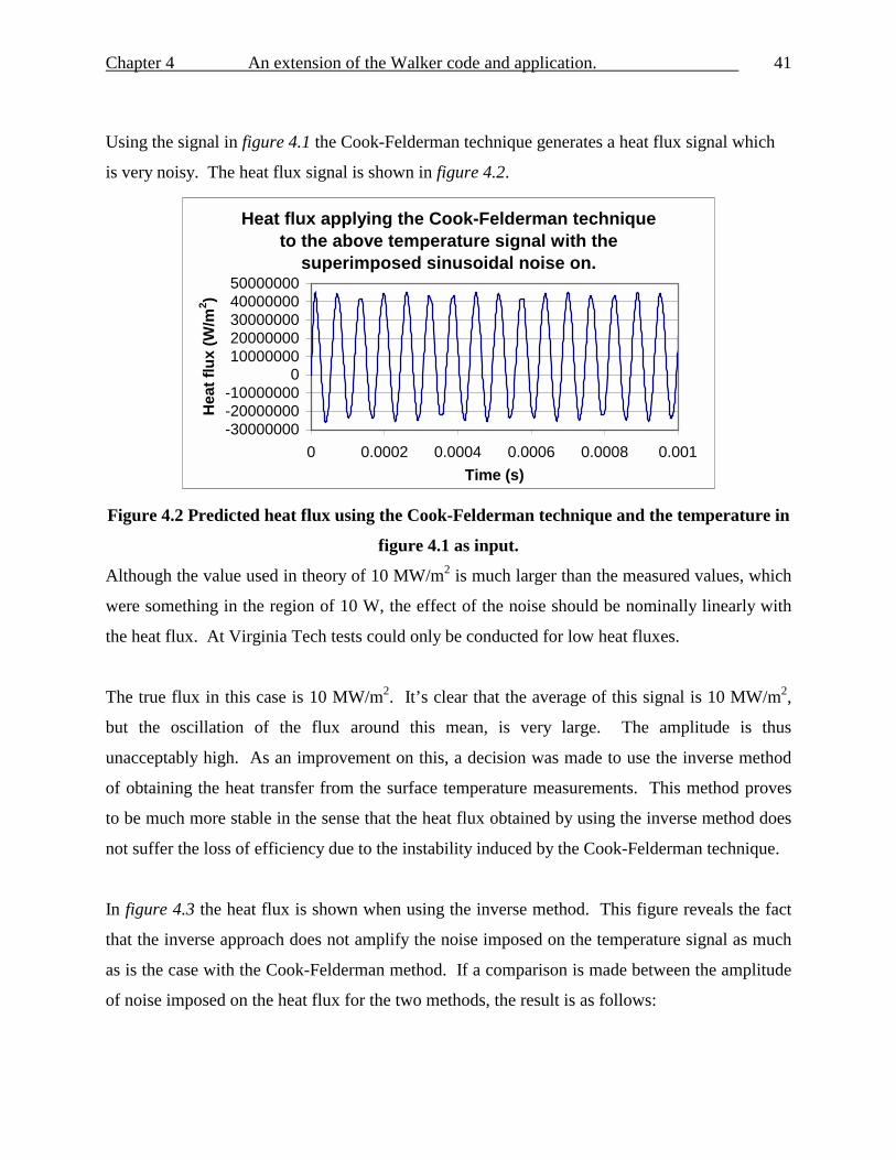
Using the signal in figure 4.1 the Cook-Felderman technique generates a heat flux signal which

is very noisy. The heat flux signal is shown in figure 4.2.

Heat flux applying the Cook-Felderman technique to the above temperature signal with the

superimposed sinusoidal noise on.

-30000000-20000000-10000000

01000000020000000300000004000000050000000

0 0.0002 0.0004 0.0006 0.0008 0.001Time (s)

Hea

t flu

x (W

/m2 )

Figure 4.2 Predicted heat flux using the Cook-Felderman technique and the temperature in

figure 4.1 as input.

Although the value used in theory of 10 MW/m2 is much larger than the measured values, which

were something in the region of 10 W, the effect of the noise should be nominally linearly with

the heat flux. At Virginia Tech tests could only be conducted for low heat fluxes.

The true flux in this case is 10 MW/m2. It’s clear that the average of this signal is 10 MW/m2,

but the oscillation of the flux around this mean, is very large. The amplitude is thus

unacceptably high. As an improvement on this, a decision was made to use the inverse method

of obtaining the heat transfer from the surface temperature measurements. This method proves

to be much more stable in the sense that the heat flux obtained by using the inverse method does

not suffer the loss of efficiency due to the instability induced by the Cook-Felderman technique.

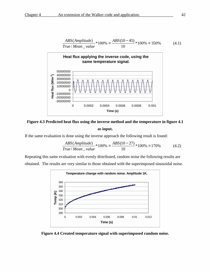
In figure 4.3 the heat flux is shown when using the inverse method. This figure reveals the fact

that the inverse approach does not amplify the noise imposed on the temperature signal as much

as is the case with the Cook-Felderman method. If a comparison is made between the amplitude

of noise imposed on the heat flux for the two methods, the result is as follows:


42

%350%100*10

)4510(%100*_/

)( =−= ABSvalueMeanTrue

AmplitudeABS (4.1)

Heat flux applying the inverse code, using the same temperature signal.

-30000000-20000000-10000000

01000000020000000300000004000000050000000

0 0.0002 0.0004 0.0006 0.0008 0.001

Time (s)

Hea

t flu

x (W

/m 2

)

Figure 4.3 Predicted heat flux using the inverse method and the temperature in figure 4.1

as input.

If the same evaluation is done using the inverse approach the following result is found:

%170%100*10

)2710(%100*_/


AmplitudeABS (4.2)

Repeating this same evaluation with evenly distributed, random noise the following results are

obtained. The results are very similar to those obtained with the superimposed sinusoidal noise.

Temperature change with random noise. Amplitude 1K.

290300310320330340350360

0 0.002 0.004 0.006 0.008 0.01 0.012

Time (s)

Tem

p (K

)

Figure 4.4 Created temperature signal with superimposed random noise.


43

As seen in the above figure the noise amplitude is much smaller than the previous theoretical

analysis in figure 4.1. This was done because the amplitude of 5K is somewhat over

conservative, but was used to show the basic effect of the noise on the eventual heat flux signal.

In the next figure, figure 4.5, the heat flux was calculated with the Cook-Felderman method.

Heat flux with Cook-Felderman and random noise with amplitude 1K.

0

5000000

10000000

15000000

20000000

0 0.002 0.004 0.006 0.008 0.01 0.012

Time (s)

Figure 4.5 The flux for the temperature in figure 4.4 using Cook-Felderman.

If the same calculation is done with the inverse method, the heat flux signal looks much better.

The frequency as well as the amplitude of the noise is less, than that predicted by the simple

superposition of the sinusoidal noise on the temperature signal. See figure4.6 for the flux

calculated with the inverse method.

Heat flux 10MW/m2, with random noise with amplitude 1K.

0

5000000

10000000

15000000

20000000

0 0.002 0.004 0.006 0.008 0.01 0.012

Time (s)

Figure 4.6 The flux for the temperature in figure 4.4 using the inverse approach.


44

%25%100*10

)5.1210(%100*_/


AmplitudeABS (4.3)

In comparison with the values in eq. 4.1 and 4.2 this value of 25% is a good improvement on the

noise amplitude in the results. It is, therefore, clear that an increase in the frequency, as well as

an increase in the amplitude of the noise on the temperature signal, will affect the output

negatively. The inverse method suppresses the amplitude of the noise through the introduction

of relaxation and bias in the code.

4.3. Experimental test case

By using some data obtained from the Cascade Tunnel at Virginia Tech, a few case studies were

made. The objective of these case studies were:

• = to remove the semi-infinite solid approach and make the application of the method for

estimating heat flux more universal. This includes the modification to the code to be

able to utilize a time dependent internal boundary condition, and not only a specified

constant temperature.

• = to compare the newly developed results to those from a commercial heat flux gage.

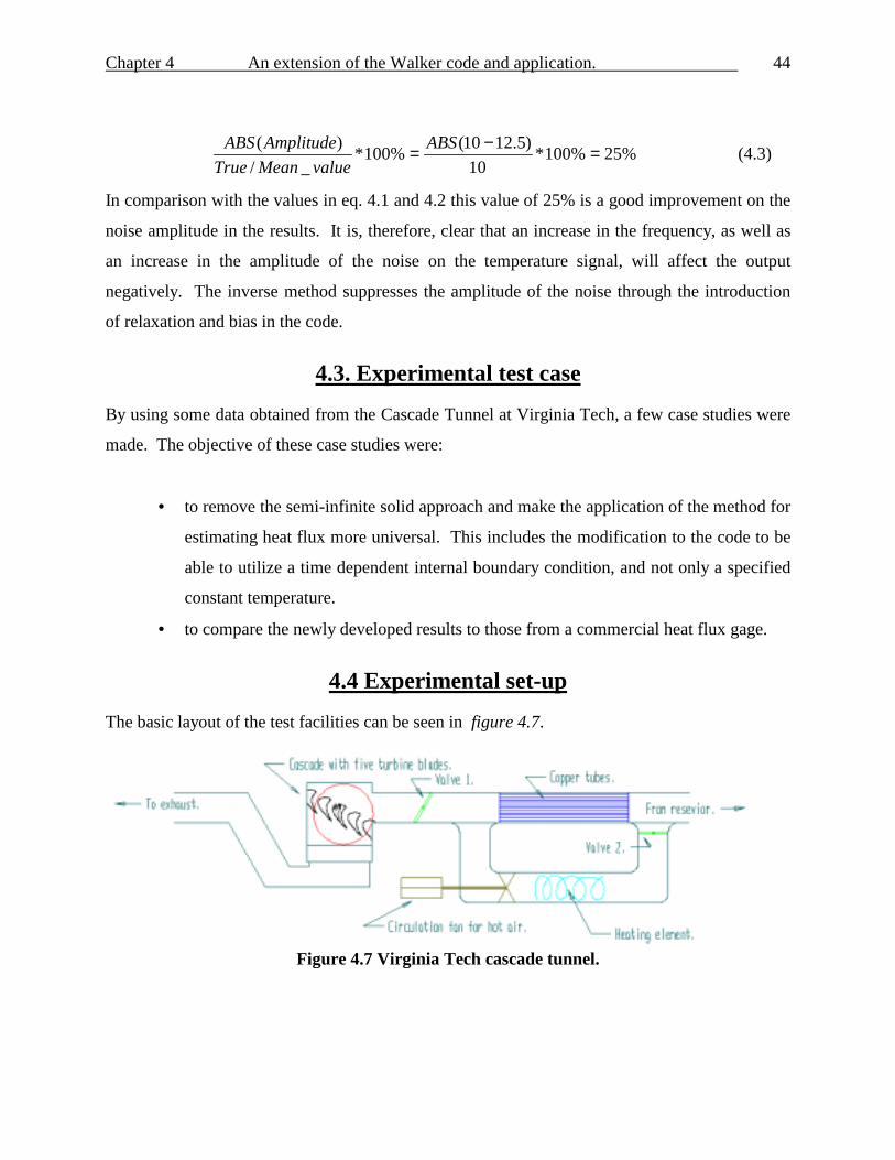
4.4 Experimental set-up

The basic layout of the test facilities can be seen in figure 4.7.

Figure 4.7 Virginia Tech cascade tunnel.


45

See this web-page for further detail on these facilities:

http://www.aoe.vt.edu/aoe/physical/cascade.html

The heating element warms the air while it is circulated through the loop system. Valve 1 is

closed and valve 2 is opened. Heat is then transferred to the copper tubes by means of

convection. The instant before the tunnel is run, valve 1 is opened and valve 2 is closed. The air

from the reservoir is then heated as it runs through the hot copper tubes. This hot air then runs

through the cascade and out the exhaust. Photos of the blade in the cascade tunnel are shown in

figure 4.8 and 4.9. See Appendix C for more photos of the cascade tunnel facilities.

Figure 4.8 Instrumented blades in the cascade tunnel.


46

Figure 4.9 The blades in the tunnel with the film-cooling-air pipe.

A 3-D view of the blade is shown in figure 4.10.

Figure 4.10 A 3-D view of the test blade.

In figure 4.11 the schematic layout of the two thermocouples installed in the blade is shown.

The distance between the two thermocouples is 25mm. Wires to both of these gages run through

a hole in the side of the blade and out through the wall of the cascade tunnel.


47

Figure 4.11 The blade with the two thermocoup

There were two aluminum blades used in these experiments.

instrumented with six thermocouples, six HFS heat flux gages

sensors. The thermocouples in this blade were Copper/Consta

Another similar blade was used but with only one of each of the

(see figure 4.7.) In this blade, another thermocouple was insta

thermocouples. This thermocouple was custom made by the

thermocouple is not a conventional one, because it’s made from a

The reason why aluminum was used was to match the ther

aluminum blade that will carry the thermocouple in one test appl

This will ensure that the heat flux through the thermocouple itself

achievable to the actual flux through the body. The blade is made

thermocouple is made of 3003 aluminum. The thermophysical

given in Table 4.1.

Surface thermocouple

position.

The second thermocouple,

for measuring the back face

temperature or the interior

temperature.

25mm

A small channel in the blade for

electrical wires.

le positions.

The first blade was fully

[26] and six Kulite pressure

ntan, also known as type K.

gages installed at the surface

lled in addition to the type K

“Medtherm” company. This

luminum (Al) and Constantan

mophysical properties of the

ication, as closely as possible.

will be as close as practically

of 6061 aluminum alloy. The

properties of these alloys are


48

Table 4.1 Comparison of properties between the model blade and the thermocouple.

Blade Thermocouple Aluminum Alloy 6061 3003

Density kg/m^3 2700 2720

Conductivity W/m.K 155 - 180 162

Specific heat J/kg.K 896 893

The basic concept of the thermocouple is visible in Figure 4.12.

Figure 4.12 Al-C

As seen from Figure 4.12, the thermocoupl

very thin constantan wire on the inside. A

the two conductors. The electrical connectio

a thin film (≈1µm) of Al on the top. The

time of the thermocouple. This thermocou

The distance between the surface and back

code this distance is divided into 100 grid

convenient number. The spacing is 0.2

convergence increases dramatically.

0.030”

onstantan thermocouple.

e is made from a small Al tube on the outside and a

thin ceramic insulator tube (Alumina) then separates

n on top of the thermocouple, is made by depositing

thinner the connecting layer, the faster the response

ple will be used to measure the surface temperature.

face thermocouples is approximately 25mm. In the

points. This gives a fairly fine grid, but is also a

5mm. If this number is increased, the time to


49

The temperature inside the blade was measured with a type-K thermocouple glued to the metal

with a metal epoxy.

Conventional thermocouples usually make use of an electronic ice bath built into the computer.

In this case it was not possible because of the unusual thermocouple metal pair used, therefore a

real ice bath was used to create the reference temperature of 0 0C.

Figure 4.13 Experimental set-up

Figure 4.13 shows the basic ice-bath set-up. The voltage meas

proportional to the difference in the temperature between the b

bath is at 0 0C, which makes it a very appropriate reference temp

data was taken was 100Hz. This particular value was chosen bec

were done at this frequency, and the same LabView program wa

from the heat flux gages, pressure gages, thermocouples etc. T

domain of output voltage from the thermocouple was 39.6µV/oC.

In figure 4.14 below, the measured temperature on the surfa

thermocouple as well as the measured temperature at the speci

given as a function of time.

.

.

.

Constantan wire

.

ured by the computer is d

lade and the ice-bath. T

erature. The frequency at

ause all the other measur

s used to accumulate all t

he calibration factor used

(Supplied by Medtherm)

ce as given by our alu

fied depth below the sur

Blade

Ice-bath at 00C.

Aluminum wires
Computer.
irectly

he ice-

which

ements

he data

in the

minum

face is


50

Temperatures.

2022

2426

2830

32

0 10 20 30

Time (s)

Tem

pera

ture

(C)

Surface temperature.

Back facetemperature.

Figure 4.14 Measured surface and internal temperature.

Keeping this graph in mind and using the original Walker code to calculate the heat flux through

the wall and into the object, the temperature profile at a specific depth beneath the surface can be

calculated assuming a semi-infinite body. If this depth is equal to the distance to the back face,

the temperature profile should correspond to the measured profile at the back. This is not the

case beyond about 12 seconds, and the deviation can be seen in figure 4.15. This discrepancy is

caused by the fact that the original code uses a semi-infinite solid approach.

Measured and calculated inner temperature.

301301.5

302302.5

303303.5

304304.5

305

0 2 4 6 8 10 12 14 16 18 20 22

Time in s.

Tem

pera

ture

in K

Measured inner temperature

Calculated inner temperatureassuming semi-infinite body.

Figure 4.15 Difference between the measured and calculated temperature, using the

original code that assumes semi-infinite body.


51

The HFS heat flux gage is also able to measure a temperature, using a platinum resistance

thermometer. The electric resistance changes with temperature, and the voltage output can then

be related to the temperature on the surface. This temperature, the RTS temperature, is graphed

in figure 4.16. The HFS gage consists of a number of thermocouples connected in series across a

thin thermal resistance layer [14]. This is done to amplify the voltage output from the gage.

Figure 4.16 RTS surface temperature.

When comparing the RTS and the aluminum thermocouple temperatures, there is a slight

difference as shown in figure 4.17. A possible error might be a delay in the RTS temperature

measured, because of the larger thermal mass associated with the heat flux gage. The sensitivity

of the Medtherm thermocouple is very good. This is achieved with the thin connecting layer on

top. The response times are also very fast, and claims by Medtherm are in the order of 1 µs.

This is faster than is possible with most of the other conventional heat flux gages. These

thermocouples have been used in the past for the measurement of temperature in gun barrels.

Under these extreme conditions, Medtherm claims that they performed well [23].

RTS temperature.

20

22

24

26

28

30

32

0 10 20 30 40Time (s)

RTS temperature.


52

Temperature comparison.

20

22

24

26

28

30

32

0 10 20 30 40Time (s)

Medtherm tempRTS temp

Figure 4.17 Comparison of the RTS and coaxial surface temperatures.

The heat flux measured by the HFS gage is presented in figure 4.18, below. In the figure, data

acquisition started at time zero. The moment heated air started to flow, (the tunnel is being

turned on) the curve shows measurable values of heat flux after approximately 3 seconds. The

maximum of this curve is approximately 5 W/cm2, and this maximum is at 4.2s.

HFS heat flux gage.

-2-10123456

0 5 10 15 20 25 30

Time (s)

Hea

t flu

x (W

/cm

2 )

Figure 4.18 HFS heat flux.

First, the heat flux obtained by using the measured temperature profile in figure 4.18 in a simple

implicit finite difference method ( Class 2 ) was used to see if the answers are in the same range.

This is a normal finite difference method, using the two measured temperatures (the coaxial

thermocouple and the type-K thermocouple temperatures) as the boundary conditions. In this and


53

the next approaches, the time step and the spacing were the same as in all the other cases. ∆x =

0.25mm and ∆t = 0.01s. Due to the noise that gets amplified, an answer is fairly difficult to

achieve. In the graph an average was calculated for the noisy heat flux – the average of every ten

points of a total of 30000 points were calculated. This average gives a much more reasonable

answer.

Heat flux with FDM

-4-202468

1012

0 5 10 15 20 25 30

Time (s)

Hea

t flu

x (W

/cm

2 )

Figure 4.19 Heat flux predicted with a simple implicit finite difference (Class 2) technique.

The problem with this approach is the effects of noise and this method is fairly difficult, because

the independence of the result as a function of decreasing grid spacing converges very slowly.

However, this graph is a indication of the answer that one can expect. The sharp peak in the heat

flux is due to the sharp increase in the temperature at this point measured by the Medtherm

thermocouple. If this initial spike is ignored, for the moment, the maximum value of the flux in

this case, is on the order of 6 W/cm2, which can be compared to the HFS maximum of 5 W/cm2.

This does not mean that the spike can be ignored when we look at the global picture. The HFS

gage might smear this spike, because of its larger “footprint.”

Now, using the extended version of the Walker code, we get an answer very similar to the one in

the above figure as shown in figure 4.20. The most obvious characteristic of figure 4.20 is the

fact that the noise is much less than that produced by the finite difference method in figure 4.19.


54

The results are qualitatively similar. The maximum is approximately 6 W/cm2 compared to the

value of 5 W/cm2 from the HFS gage.

Heat flux with temperature boundary.

-4

-2

0

2

4

6

8

10

12

0 5 10 15 20 25 30Time (s)

Hea

t flu

x (W

/cm

^2)

Figure 4.20 Predicted heat flux from the extended inverse code.

Figure 4.21 Same flux as in figure 4.20 but with the Cook-Felderman technique.

Last, using the same surface temperature from the Medtherm thermocouple, but this time the

simpler Cook-Felderman technique, the predicted flux in figure 4.21 is the outcome. The blue

signal is the original and the black is an average. If one looks closely, the flux at 20s, in figure

4.20, is lower compared to that obtained in figure 4.21. This is because the internal temperature

is rising ( seen in figure 4.14), therefore the flux will be less than in the semi-infinite solid case

as assumed in the Cook-Felderman method. In the semi-infinite solid case, the temperature in the

middle of the blade is assumed to be constant. In reality this is not the case. The temperature

does rise, and the slope of the temperature profile will be slightly less, causing the flux to be less

as well.


55

4.5 Conclusions

Looking at all the graphs in this chapter, it is clear that the flux estimated by the new code is

somewhat higher than that suggested by the calibrated HFS heat flux gages. On the other hand

the flux obtained from the RTS temperature from the HFS gage, through the Cook-Felderman

scheme, gives a very similar numerical value to the flux up until the time where the semi-infinite

assumption in the Cook-Felderman method is no longer valid. This is due to the fact that the

temperature profiles are very similar. The HFS gages are calibrated to give a certain voltage for

a certain heat flux. The calibration is, however, subject to errors.

A potential cause for the discrepancies is that the heat flux is assumed to be 1-D in all cases. It

is important to keep in mind that 2-D heat flow might be of such a great effect that the flux

obtained numerically through the evaluation of the surface temperatures, is not reliable. In the

next chapter, 2-D effects will be evaluated to see whether they are of substantial importance or

not.

DEPARTMENT OF AEROSPACE AND OCEAN

ENGINEERING

Transonic Cascade Wind Tunnel

The Virginia Tech Transonic Cascade Wind Tunnel is a blow down transonic facility capable of a twenty second run time.An overall layout is given in Figure X, and a photo is shown in Figure Y. The air supply is pressurized by a four-stageIngersoll-Rand compressor and stored in large outdoor tanks. The maximum tank pressure used for transonic tests is about1725 kPa (250 psig).

Figure X. Transonic Cascade Wind Tunnel Layout

Department of Aerospace and Ocean Engineering

http://www.aoe.vt.edu/aoe/physical/cascade.html (1 of 3) [11/30/2000 10:27:58 AM]

http://www.vt.edu/

Figure Y. Photograph of the Cascade Wind Tunnel Test Section

During a run, the upstream total pressure is held constant by varying the opening of a butterfly valve controlled by acomputerized feedback circuit. There is also a safety valve upstream of the control valve to start and stop the tunnel. Thetest section area is 37.3 cm high, and is designed for blades with an outlet angle of approximately 70 degrees. The bladeisentropic exit Mach number is varied by changing the upstream total pressure; the usual range for exit Mach number is0.7 to 1.35. The throat Reynolds number for typical tests is 340,000.



Figure Z. Typical Test Section Diagram

Figure Z is a diagram of the test section. The tunnel mean flow is left to right on the figure, and is turned through 68degrees by the blade passages, which act as the tunnel throat. Upstream of the blades, the bundle of three shock shapersprotrudes from the test section top block; the shocks propagate down from the shaper exit to the bottom of the test section.The high-response total pressure probe for downstream surveys is also shown on the figure, pointing into the cascade exitflow. The probe moves up and down in line with wall static pressure taps. No tailboard is used downstream of the cascade,which means that a free shear layer forms between the exit plane of the blades and the test section back wall. Note also theupstream total pressure probe, which is fixed at mid-pitch of the “Lower” passage.

Back to FacilitiesBack to High-Speed Flow Research

Send comments and suggestions [email protected]

Copyright © 1996 AOE Dept., Virginia Tech All rights reserved world wide



http://www.aoe.vt.edu/aoe/physical/facil.html

http://www.aoe.vt.edu/aoe/research/hispdflo/hispdflo.html

mailto:[email protected]

4.1 Extending the Walker code - Virginia Tech

Documents

Transcript of 4.1 Extending the Walker code - Virginia Tech