4. SYNTHESIS of AUTOMATIC CONTROL SYSTEMS

As synthesis of the automatic control systems, the design of a system proceeded from

pre-determined requirements is meant. The synthesis is more complicated process

than it is the analysis of an existing system, therefore that the synthesis does not have

a unique solution, so as to the same result different methods could lead - for example

the structure of the system or the control algorithms could be varied. In one case, one

has to deal with the solution on the energy level, in the second case on the information

level, [2].

Here it is suitable to repeat the formulation of the control task – the objective of the

control is to take the definition point of the system from initial point A to the point B,

according to the control task; satisfying quality requirements simultaneously. An

essential abstract here is, that the motion in the state space does not mean the

geographical change of a mechanism’s parts, but the change of quantities describing

entire state of the system.

An automatic control system is usually designed around a previously known control

object, a motor, for instance. If the parameters of the object are known in advance,

then in the design process only the regulator parameters are determined, or the

regulator will be synthesised.

The synthesis of the regulator is required in three cases

� The system is structurally unstable

� the accuracy of the system is not sufficient

� the transient processes of the system do not scope with quality requirements

Earlier the trial-and-error method was used in the synthesis, which had set higher

requests to the designers, however, the development of the computer technology

enables preliminary simulation of systems, reducing the cost of the systems and

requests to the designers. Simulation could be made by various software, MatCad,

MATLAB, etc. for instance, That enables carry out the calculations as in the time so

in frequency and in state spaces, but on the background of all of it one must not

forget, that simulations could be inaccurate (look division 3.3.1.4.)

4.1. Selection of the suitable regulator.

The following consideration holds for simple automatic control systems. Connecting

together a stable control object and stable control device might not give a stable

system. The same time while connection of two unstable devices might give a stable

system. From this, the complexity of the synthesis could be understood, wherefore in

the practice certain system configuration are widespread, which provide structural

stability in case of negative feedback [3].

Table 4.1. Structurally stable systems

Obj. P PT1 PT2 I IT1 P PT1 I P PT1 P P PT1

Reg. P P P P P PT1 PT1 PT1 I I IT1 PI PI

In the design process the regulator will be selected so, that the parameters of the

regulator, lying in given limits, provide the stability of the system. Thereby the rule is

taken into account, that the order of the regulator must not exceed the order of the

control object. The reason of this rule could be explained as follows:

For each order there corresponds one time constant in the system, and the more time

constants are in the system, the slower, and vibratory is the system. The system time

constants are compensated by regulators, or they are attempted to be reduced out. In

case if for the control of a second order system a third order regulator will be used,

then one more time constant will be implemented into the system, in addition of two

existing already, which were attempted to reduce, or - the regulation is not as efficient

as it could be.

4.2. Comparison of different regulators

To investigate most widespread PID-family regulators like P, PI, and PID it is suitable

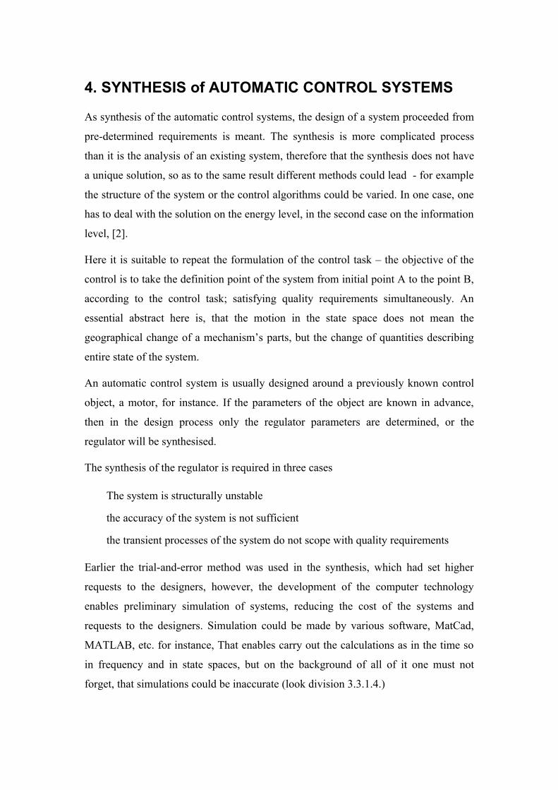
to use a PT3 control object, parameters of which were K1 = K2 = K 3 = 1, T1 = 5 s, T2 =

1 s, T3 = 0.2 s. Such automatic control system is represented in the figure 4.1.

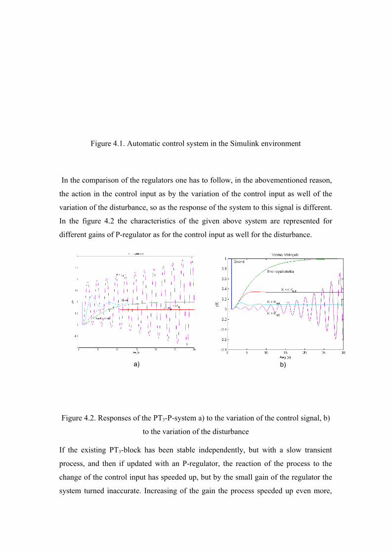
Figure 4.1. Automatic control system in the Simulink environment

In the comparison of the regulators one has to follow, in the abovementioned reason,

the action in the control input as by the variation of the control input as well of the

variation of the disturbance, so as the response of the system to this signal is different.

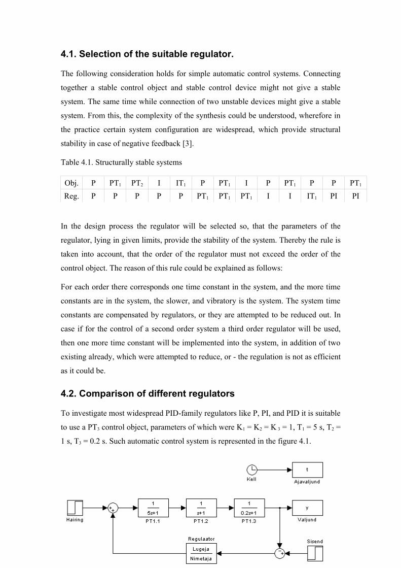
In the figure 4.2 the characteristics of the given above system are represented for

different gains of P-regulator as for the control input as well for the disturbance.

Figure 4.2. Responses of the PT3-P-system a) to the variation of the control signal, b)

to the variation of the disturbance

If the existing PT3-block has been stable independently, but with a slow transient

process, and then if updated with an P-regulator, the reaction of the process to the

change of the control input has speeded up, but by the small gain of the regulator the

system turned inaccurate. Increasing of the gain the process speeded up even more,

a) b)

also the accuracy has improved, but the vibratory processes with over-regulation

arose, which in some cases are undesired. With further increase of the regulator’s gain

the stability margin will be exceeded and the output will oscillate with increasing

amplitude, the mean of which presents the desired output value.

Considering the reaction of the system to a disturbance by given gains of regulators

on might see, that the reaction speed does not depend on the regulators, however, the

regulator is able to compensate the impact of the disturbance in certain limits, not

being able to reduce this impact to zero. Compensation is the more efficient the grater

is the regulator’s gain, but this will involve oscillating processes.

Figure 4.3. Response of a PT3-block and different regulators to the a) control,

b) disturbance

Comparing P-regulator with other regulators one can see, that the regulators with I-

block are accurate or they reach the set value of the system in the output, but they are

inevitably accompanied with oscillating process. The same happens by the response to

the disturbance, where the regulators with I-block are able to compensate its impact

fully. Comparing PI-regulators with PID regulators one has to mention as a difference

the fact, that D-block provides faster response, although it is not clearly to see in

examples given.

Causal actions of parts of a PID-regulator .are explained in the figure 4.5. Provided

that the control object (figure 4.4.) was previously operating in a settled mode without

a) b)

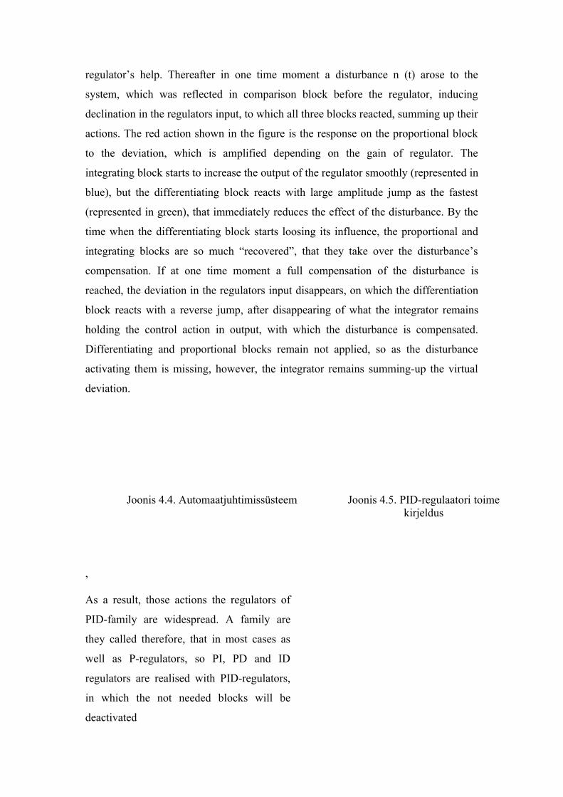
regulator’s help. Thereafter in one time moment a disturbance n (t) arose to the

system, which was reflected in comparison block before the regulator, inducing

declination in the regulators input, to which all three blocks reacted, summing up their

actions. The red action shown in the figure is the response on the proportional block

to the deviation, which is amplified depending on the gain of regulator. The

integrating block starts to increase the output of the regulator smoothly (represented in

blue), but the differentiating block reacts with large amplitude jump as the fastest

(represented in green), that immediately reduces the effect of the disturbance. By the

time when the differentiating block starts loosing its influence, the proportional and

integrating blocks are so much “recovered”, that they take over the disturbance’s

compensation. If at one time moment a full compensation of the disturbance is

reached, the deviation in the regulators input disappears, on which the differentiation

block reacts with a reverse jump, after disappearing of what the integrator remains

holding the control action in output, with which the disturbance is compensated.

Differentiating and proportional blocks remain not applied, so as the disturbance

activating them is missing, however, the integrator remains summing-up the virtual

deviation.

,

As a result, those actions the regulators of

PID-family are widespread. A family are

they called therefore, that in most cases as

well as P-regulators, so PI, PD and ID

regulators are realised with PID-regulators,

in which the not needed blocks will be

deactivated

Joonis 4.4. Automaatjuhtimissüsteem Joonis 4.5. PID-regulaatori toime kirjeldus

4.3. Adjustment of a PID-regulator

For the adjustment of aregulator different possibilities exist, from which one, the

analytical, was considered by petermining of the stability domains. Analytical

methods usually contain calculations in considerable amount and giving as result the

ansver about suitability of the stability domain or parameters configuration of certain

system for certain task given with initial assignment. Therefoe in the practice abstract

methods are used, which give with less calulations a prelimnary set of parameters,

which will be optimised in the further process of simulation or fitting. For the

comparison of different adjustments mutually the integral criteria are used. Below are

some most widespread in practice for the regulator’ adjustment are considered.

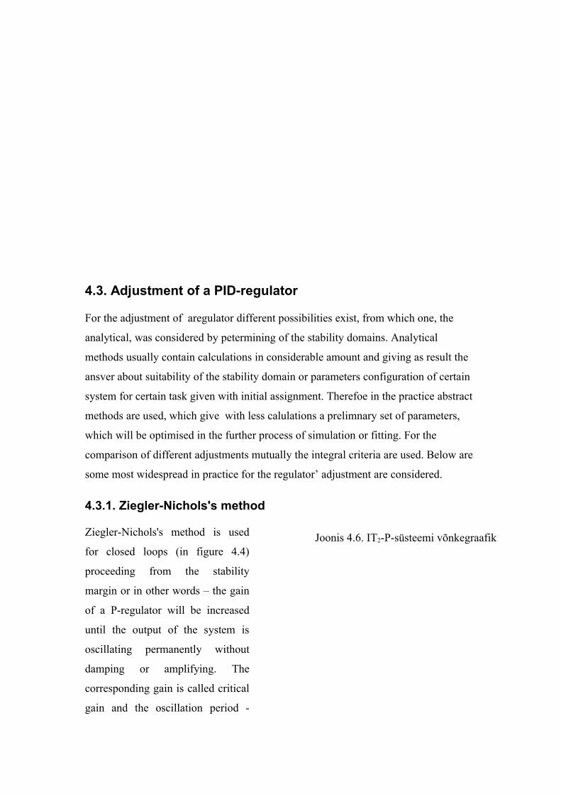
4.3.1. Ziegler-Nichols's method

Ziegler-Nichols's method is used

for closed loops (in figure 4.4)

proceeding from the stability

margin or in other words – the gain

of a P-regulator will be increased

until the output of the system is

oscillating permanently without

damping or amplifying. The

corresponding gain is called critical

gain and the oscillation period -

Joonis 4.6. IT2-P-süsteemi võnkegraafik

critical period. Equations for

calculations are given in the table

4.2. [6]

Table 4.2. Parameters of a regulator by Ziegler-Nichols.

Parameter P-regulator PI-regulator PID-regulatorKR 0.5⋅K Rkrit 0.45⋅K Rkrit 0.6⋅K Rkrit

TI - 0.83⋅T krit 0.5⋅T krit

TD - - 0.125⋅T krit

4.3.2. CHR-method

CHR in an abbreviation from the authors names – Chien, Hrones and Reswick. CHR

was developed from the Ziegler-Nichols's method for implementation of certain

quality requirements of open systems. Using the aperiodic step response, the

conditional parameters of the process will be determined [6]

� time lag of the process TH;

� time constant of the process T0;

� gain of the process KP.

Figure 4.7.Aperiodic transient process

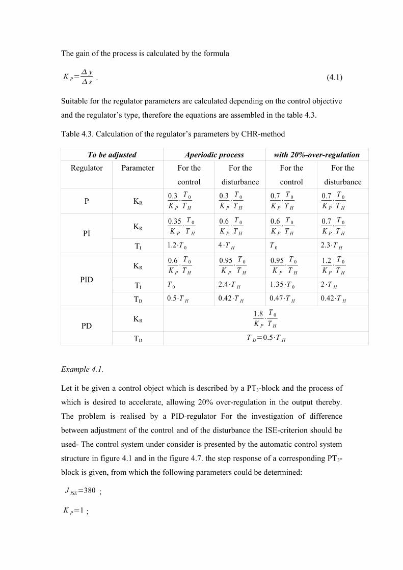
The gain of the process is calculated by the formula

K P= y s . (4.1)

Suitable for the regulator parameters are calculated depending on the control objective

and the regulator’s type, therefore the equations are assembled in the table 4.3.

Table 4.3. Calculation of the regulator’s parameters by CHR-method

To be adjusted Aperiodic process with 20%-over-regulationRegulator Parameter For the

control

For the

disturbance

For the

control

For the

disturbance

P KR0.3K P

⋅T 0

T H

0.3K P

⋅T 0

T H

0.7K P

⋅T 0

T H

0.7K P

⋅T 0

T H

PIKR

0.35K P

⋅T 0

T H

0.6K P

⋅T 0

T H

0.6K P

⋅T 0

T H

0.7K P

⋅T 0

T H

TI 1.2⋅T 0 4⋅T H T 0 2.3⋅T H

PID

KR0.6K P

⋅T 0

T H

0.95K P

⋅T 0

T H

0.95K P

⋅T 0

T H

1.2K P

⋅T 0

T H

TI T 0 2.4⋅T H 1.35⋅T 0 2⋅T H

TD 0.5⋅T H 0.42⋅T H 0.47⋅T H 0.42⋅T H

PDKR

1.8K P

⋅T 0

T H

TD T D=0.5⋅T H

Example 4.1.

Let it be given a control object which is described by a PT3-block and the process of

which is desired to accelerate, allowing 20% over-regulation in the output thereby.

The problem is realised by a PID-regulator For the investigation of difference

between adjustment of the control and of the disturbance the ISE-criterion should be

used- The control system under consider is presented by the automatic control system

structure in figure 4.1 and in the figure 4.7. the step response of a corresponding PT3-

block is given, from which the following parameters could be determined:

J ISE=380 ;

K P=1 ;

T H=0.7 s ;

T 0=7.9 s .

From the table 4.3. are selected corresponding for the performance specification

formula and found on their basis regulator’s parameters are assembled in the table 4.4.

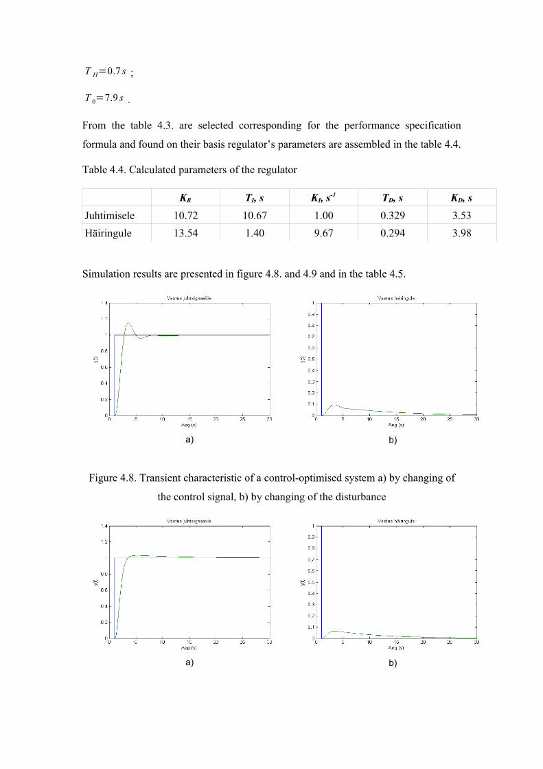
Table 4.4. Calculated parameters of the regulator

KR TI, s KI, s-1 TD, s KD, sJuhtimisele 10.72 10.67 1.00 0.329 3.53Häiringule 13.54 1.40 9.67 0.294 3.98

Simulation results are presented in figure 4.8. and 4.9 and in the table 4.5.

Figure 4.8. Transient characteristic of a control-optimised system a) by changing of

the control signal, b) by changing of the disturbance

a) b)

a) b)

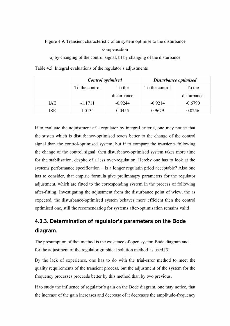
Figure 4.9. Transient characteristic of an system optimise to the disturbance

compensation

a) by changing of the control signal, b) by changing of the disturbance

Table 4.5. Integral evaluations of the regulator’s adjustments

Control optimised Disturbance optimisedTo the control To the

disturbance

To the control To the

disturbanceIAE -1.1711 -0.9244 -0.9214 -0.6790ISE 1.0134 0.0455 0.9679 0.0256

If to evaluate the adjuistment af a regulator by integral criteria, one may notice that

the susten which is disturbance-optimised reacts better to the change of the control

signal than the control-optimised system, but if to compare the transients following

the change of the control signal, then disturbance-optimised system takes more time

for the stabilisation, despite of a less over-regulation. Hereby one has to look at the

systems performance specification – is a longer regulatin priod acceptable? Also one

has to consider, that empiric formula give prelimnaqry parameters for the regulator

adjustment, which are fitted to the corresponding system in the process of following

after-fitting. Investigating the adjustment from the disturbance point of wiew, the as

expected, the disturbance-optimised system behaves more efficient then the control

optimised one, still the recomendatiog for systems after-optimisation remains valid

4.3.3. Determination of regulator’s parameters on the Bode diagram.

The presumption of thei method is the existence of open system Bode diagram and

for the adjustment of the regulator graphical solution method is used.[3]

By the lack of experience, one has to do with the trial-error method to meet the

quality requirements of the transient process, but the adjustment of the system for the

frequency processes proceeds better by this method than by two previous.

If to study the influence of regulator’s gain on the Bode diagram, one may notice, that

the increase of the gain increases and decrease of it decreases the amplitude-frequency

characteristic, not changing thereby the phase-frequency characteristic of the system.

Alternatively, it follows from here, that it is possible

to achieve with the proportional block of the

regulator the required amplitude

reserve.

The gain of a PI-regulator has similar

properties like P-regulators one.

Provided, that most of real objects are

PTn-blocks, the time constant of an

integrating block is approximated to

the largest time constant of the system.

As a result of it, one has good reaction

to the change of the control signal.

PD-regulator is used when the control

object shows integrating action. In this

case, the rising effect of the phase-

frequency characteristic are applied.

As the integration time constant was

approximated to the largest time

constant of the system, the same will

be made with differentiation time

constant

Using PID-regulator, the time constants will be adjusted to the largest time constant of

the control object, holding the condition T IT D . . Also it must be taken into account

the pirate time constants of the real integrating and differentiating blocks, which are

tried to be selected minimal possible to minimise the distortions

Joonis 4.11. PI-regulaatori Bode diagramm

Joonis 4.12. PD-regulaatori Bode diagramm

4.3.4. Amplitudoptimum

Considering an abstract

automatic control system on may

assume, that an ideal response o

the control signal was in case if

the transfer function of the

whole system W=1. In this case,

the output of the system will

follow the input of the system

exactly [9].

As process, one PTn-block could be considered, by which most of the drives in use

could be described and the transfer function of which is

W P p = 1a 0a 1⋅pa 2⋅p 2... . (4.2)

Suitable regulator for this process is PID-regulator, transfer function of which could

be represented in form

W R p =r 2⋅p 2r1⋅pr0

2⋅p. (4.3)

Bearing in mind the objective of the synthesis W =1 , the sets of equations are

elaborated for the calculation of the parameters of the equation (4.3), which

assembled in the table 4.6.

In case if the transfer function is given n the form

W P p=K P

∏i1T i⋅p , (4.4)

then, by condition that T 1≫T =∑j=2

n

T j this process could be describes as PT2-block

W P p=K P

1T 1⋅p⋅1T ⋅p (4.5)

Joonis 4.15. Automaatjuhtimissüsteem

or in situation, where T 1 , T 2≫T =∑j=3

n

T j is valid, the process could be represented

as PT3-block

W P p =K P

1T 1⋅p⋅1T 2⋅p⋅1T ⋅p .

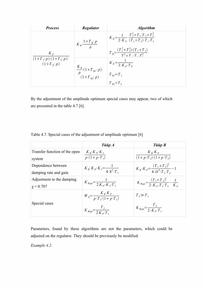
Synthesis algorithm, proceeding from this presentation is brought in table 4.6.

Table 4.6. Determination of the regulator’s parameters on the bases of amplitude

optimum

Process Regulator Algorithm

Ka 0a 1⋅pa 2⋅p 2 ...

r1⋅pr0

2⋅p

r 0=a 0⋅a1

2−a 0⋅a2

a 1⋅a 2−a 0⋅a 3

r 1=a 1⋅a 1

2−a 0⋅a 2

a 1⋅a 2−a 0⋅a 3−a0

r2⋅p 2r 1⋅pr 0

2⋅p

r 0=1∣D∣

⋅[ a 02 −a 0 0

−a 122⋅a 0⋅a 2 −a 2 a 1

a 222⋅a 0⋅a 4−2⋅a 1⋅a 3 −a 4 a 3

]r 1=

1∣D∣

⋅[a 1 a02 0

a 3 −a 122⋅a 0⋅a 2 a1

a 5 a 222⋅a0⋅a 4−2⋅a 1⋅a 3 a3

]r 2=

1∣D∣

⋅[a 1 −a 0 a 02

a 3 −a 2 −a 122⋅a 0⋅a 2

a 5 −a 4 a 222⋅a 0⋅a 4−2⋅a 1⋅a 3

]D=[a1 −a 0 0

a3 −a 2 a 1

a5 −a 4 a 3]

K P

1T 1⋅p⋅1T ⋅p K R⋅1T R⋅p

p

K R=1

2⋅K P⋅T

T R=T 1

Process Regulator Algorithm

K P

1T 1⋅p⋅1T 2⋅p⋅1T ⋅p

K R⋅1T R⋅p

p

K R=1

2⋅K P⋅

T 12T 1⋅T 2T 2

2

T 1T 2⋅T 1⋅T 2

T R=T 1

2T 22⋅T 1T 2

T 12T 1⋅T 2⋅T 2

2

K R

p⋅1T R1⋅p⋅

1T R2⋅p

K R=1

2⋅K P⋅T

T R1=T 1

T R2=T 2

By the adjustment of the amplitude optimum special cases may appear, two of which

are presented in the table 4.7 [6].

Table 4.7. Special cases of the adjustment of amplitude optimum [6]

Tüüp A Tüüp BTransfer function of the open

system

K R⋅K P⋅K I

p⋅1 p⋅T 1K R⋅K P

1 p⋅T 1⋅1p⋅T 2

Dependence between

damping rate and gainK R⋅K P⋅K I=

14⋅2⋅T 1

K R⋅K P=T 1T 2

2

4⋅D 2⋅T 1⋅T 2

−1

Adjustment to the damping

χ = 0.707K Ropt=

12 K P⋅K I⋅T 1

K Ropt=T 1T 2

2

2⋅K P⋅T 1⋅T 2− 1

K P

Special cases

W 0=K R⋅K P

p⋅T I⋅1 p⋅T 1

K Ropt=T I

2 K P⋅T 1

T 2≫T 1

K Ropt=T 2

2⋅K P⋅T 1

Parameters, found by these algorithms are not the parameters, which could be

adjusted on the regulator. They should be previously be modified.

Example 4.2.

In the synthesis process of a PID-regulator the transfer function of the regulator was

found as

W R p =r 2⋅p 2r1⋅pr0

2⋅p=

r 2

2⋅p

r1

2

r0

2⋅p.

The transfer function of a real regulator is given in the form

W RR p=K PK I

pK D⋅p ,

parameters of which could be found by the comparison of the transfer function

coefficients.

K P=r1

2 , K I=r0

2 , K D=r2

2 .

4.4. Synthesis of MIMO systems

Devices and drives are widely spread in the industry, by which a number of output

variables, which in turn could be internally dependent, are controlled simultaneously.

Digital regulators are suitable for these systems, for the synthesis of which matrix and

vector calculus are used, however, in some cases, cascade regulation, for instance, the

synthesis could be made as in time space as well in the frequency space also.

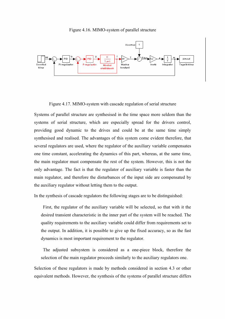
Figure 4.16. MIMO-system of parallel structure

Figure 4.17. MIMO-system with cascade regulation of serial structure

Systems of parallel structure are synthesised in the time space more seldom than the

systems of serial structure, which are especially spread for the drivers control,

providing good dynamic to the drives and could be at the same time simply

synthesised and realised. The advantages of this system come evident therefore, that

several regulators are used, where the regulator of the auxiliary variable compensates

one time constant, accelerating the dynamics of this part, whereas, at the same time,

the main regulator must compensate the rest of the system. However, this is not the

only advantage. The fact is that the regulator of auxiliary variable is faster than the

main regulator, and therefore the disturbances of the input side are compensated by

the auxiliary regulator without letting them to the output.

In the synthesis of cascade regulators the following stages are to be distinguished:

� First, the regulator of the auxiliary variable will be selected, so that with it the

desired transient characteristic in the inner part of the system will be reached. The

quality requirements to the auxiliary variable could differ from requirements set to

the output. In addition, it is possible to give up the fixed accuracy, so as the fast

dynamics is most important requirement to the regulator.

� The adjusted subsystem is considered as a one-piece block, therefore the

selection of the main regulator proceeds similarly to the auxiliary regulators one.

Selection of these regulators is made by methods considered in section 4.3 or other

equivalent methods. However, the synthesis of the systems of parallel structure differs

from the synthesis of the systems of serial structure, therefore, that different parallel

structures are distinguished [6]:

� forward or P-structure,

� reversed or V-structure.

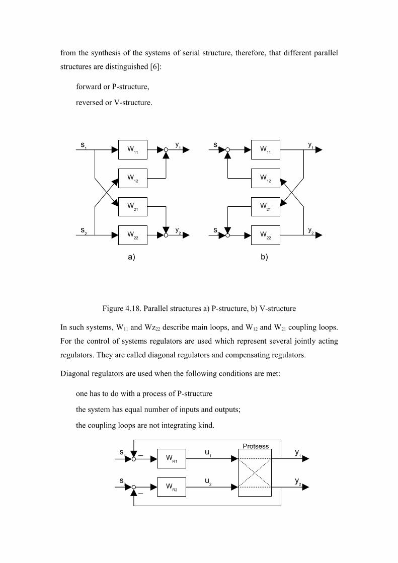
Figure 4.18. Parallel structures a) P-structure, b) V-structure

In such systems, W11 and Wz22 describe main loops, and W12 and W21 coupling loops.

For the control of systems regulators are used which represent several jointly acting

regulators. They are called diagonal regulators and compensating regulators.

Diagonal regulators are used when the following conditions are met:

� one has to do with a process of P-structure

� the system has equal number of inputs and outputs;

� the coupling loops are not integrating kind.

W11

W12

W21

W22

s1

s2

y1

y2

W11

W12

W21

W22

s1

s2

y1

y2

a) b)

WR1

WR2

s2

s1

u1

y1

u2

y2

Protsess_

_

Figure 4.19. System with diagonal regulator

Diagonal matrix inherits its name from the presentation mode f the matrix of the

system regulator.

W R=[W R1 00 W R2] . (4.6)

The synthesis of the diagonal matrix is easier than of the compensating regulator,

containing the following stages:

� determination of main loops

� selection of regulators.

� assignment of the regulator’s parameters.

Under the determination of main loops the operation is meant, where it will be

arranged which input entity imposes most directly which output variable, or

considering figure 4.20, when it was arranged that s1 imposes y1 directly and s2

imposes y2, although it could be arranged opposite, – that s1 imposes y2. In this case,

the locations of the transfer functions in the figure will change, system by itself do not

change.

By the selection of regulators one precedes similarly to the synthesis of one-loop

systems, just the determination of the parameters is made on the different basis. First,

the static coupling factor of the process will be determined

S0=W 120 ⋅W 210W 110 ⋅W 220

. (4.7)

Following, the transfer function of the main loops are determined, conceiving, that

another main loop does not exist

W 1=W R1⋅W 11

1W R1⋅W 11, (4.8)

W 2=W R2⋅W 22

1W R2⋅W 22. (4.9)

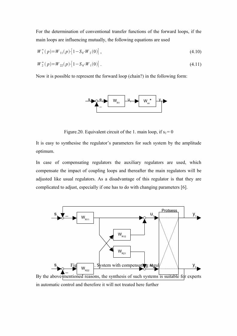
For the determination of conventional transfer functions of the forward loops, if the

main loops are influencing mutually, the following equations are used

W 1∗ p=W 11 p⋅[1−S0⋅W 2 0 ] , (4.10)

W 2∗ p=W 22 p⋅[1−S 0⋅W 10 ] . (4.11)

Now it is possible to represent the forward loop (chain?) in the following form:

Figure.20. Equivalent circuit of the 1. main loop, if s2 = 0

It is easy to synthesise the regulator’s parameters for such system by the amplitude

optimum.

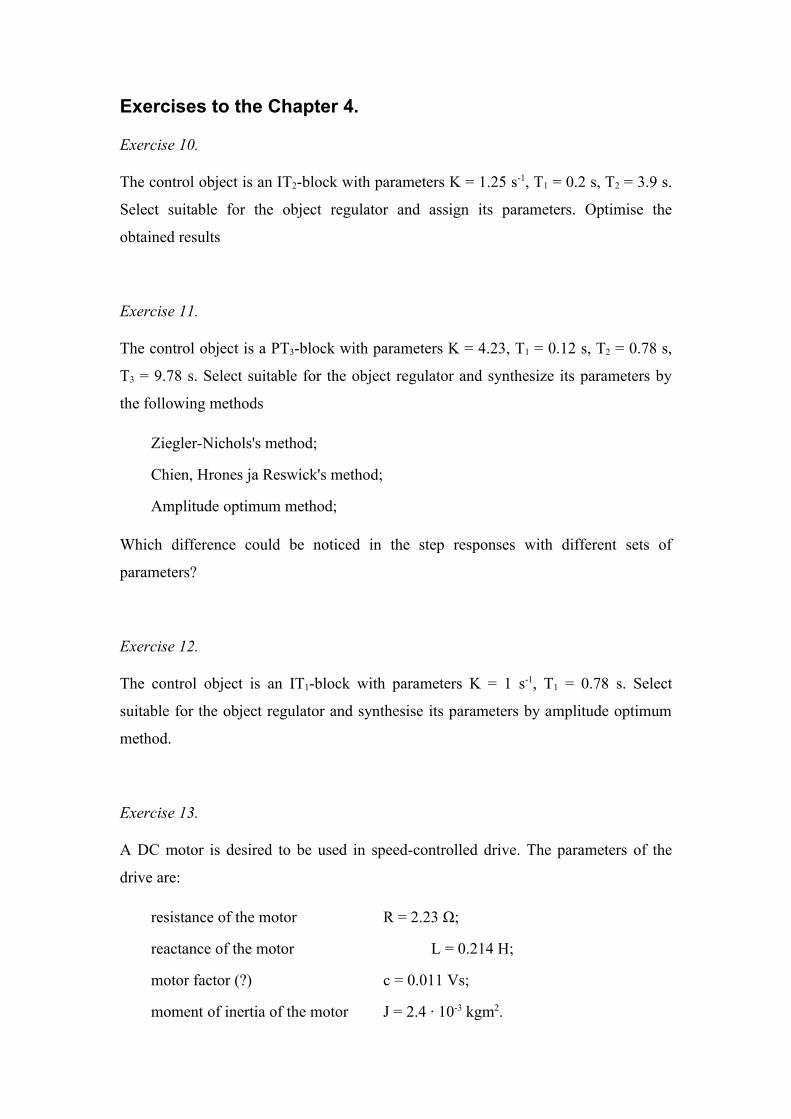
In case of compensating regulators the auxiliary regulators are used, which

compensate the impact of coupling loops and thereafter the main regulators will be

adjusted like usual regulators. As a disadvantage of this regulator is that they are

complicated to adjust, especially if one has to do with changing parameters [6].

Figures 4.21. System with compensating regulator

By the above-mentioned reasons, the synthesis of such systems is suitable for experts

in automatic control and therefore it will not treated here further

WR11

WR22

s2

s1

u1

y1

u2

y2

Protsess_

_

WR12

WR21

WR1 W

xx*s

1y1

u1

e1

_

Exercises to the Chapter 4.

Exercise 10.

The control object is an IT2-block with parameters K = 1.25 s-1, T1 = 0.2 s, T2 = 3.9 s.

Select suitable for the object regulator and assign its parameters. Optimise the

obtained results

Exercise 11.

The control object is a PT3-block with parameters K = 4.23, T1 = 0.12 s, T2 = 0.78 s,

T3 = 9.78 s. Select suitable for the object regulator and synthesize its parameters by

the following methods

� Ziegler-Nichols's method;

� Chien, Hrones ja Reswick's method;

� Amplitude optimum method;

Which difference could be noticed in the step responses with different sets of

parameters?

Exercise 12.

The control object is an IT1-block with parameters K = 1 s-1, T1 = 0.78 s. Select

suitable for the object regulator and synthesise its parameters by amplitude optimum

method.

Exercise 13.

A DC motor is desired to be used in speed-controlled drive. The parameters of the

drive are:

� resistance of the motor R = 2.23 Ω;

� reactance of the motor L = 0.214 H;

� motor factor (?) c = 0.011 Vs;

� moment of inertia of the motor J = 2.4 · 10-3 kgm2.

In the calculations the effects of the load and electro-motor force could be omitted, also the distortions induced by the time lag of the power converter. Such system is represented in the figure 4.17. For the control of current use the P-regulator and also for the speed P-regulator. Synthesise parameters of these regulators