
4 Interrupted flow HCM 2010 - ТФБ€¦ · 16.4.2015 1 Traffic engineering Highway Capacity...
37
16.4.2015 1 Traffic engineering Highway Capacity Manual 2010 Interrupted traffic flow Dr. Drago Sever 2 Content Interrupted traffic flow Intersections Two‐way STOP controlled intersections (TWSC) Roundabouts Signalized intersection Examples – urban streets (HCS 2010)
Transcript of 4 Interrupted flow HCM 2010 - ТФБ€¦ · 16.4.2015 1 Traffic engineering Highway Capacity...
16.4.2015
1
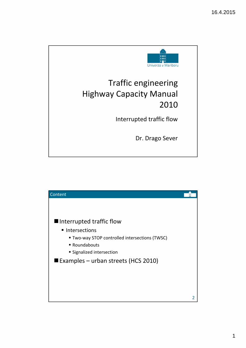
Traffic engineeringHighway Capacity Manual
2010
Interrupted traffic flow
Dr. Drago Sever
2
Content
Interrupted traffic flow Intersections Two‐way STOP controlled intersections (TWSC)
Roundabouts
Signalized intersection
Examples – urban streets (HCS 2010)
16.4.2015
2
Organization of HCM
HCM 2010
3
Volume 1 – ConceptsVolume 2 – Uninterrupted Flow Facilities
Freeways, rural highways, rural roadsVolume 3 – Interrupted Flow Facilities
Urban arterials, intersections, roundaboutsSignals at freeway interchanges,Bicycle and Pedestrian paths
Volume 4 – Supplemental Materials (Website)
http://www.hcm.trb.org
NEW
Urban street segments and facilities Chapter 16: Urban street facilities
Chapter 17: Urban street segments
Intersections Chapter 18: Signalized intersection
Chapter 19: TWSC intersection
Chapter 20: AWSC intersection
Chapter 21: Roundabouts
Chapter 22: Interchange ramp terminal
Off‐street pedestrian an bicycle facilities Chapter 23: Off‐street P&B facilities
Volume 3: Interrupted flow
HCM 2010
4
16.4.2015
3
HCM 2010 – TWSC intersections
5
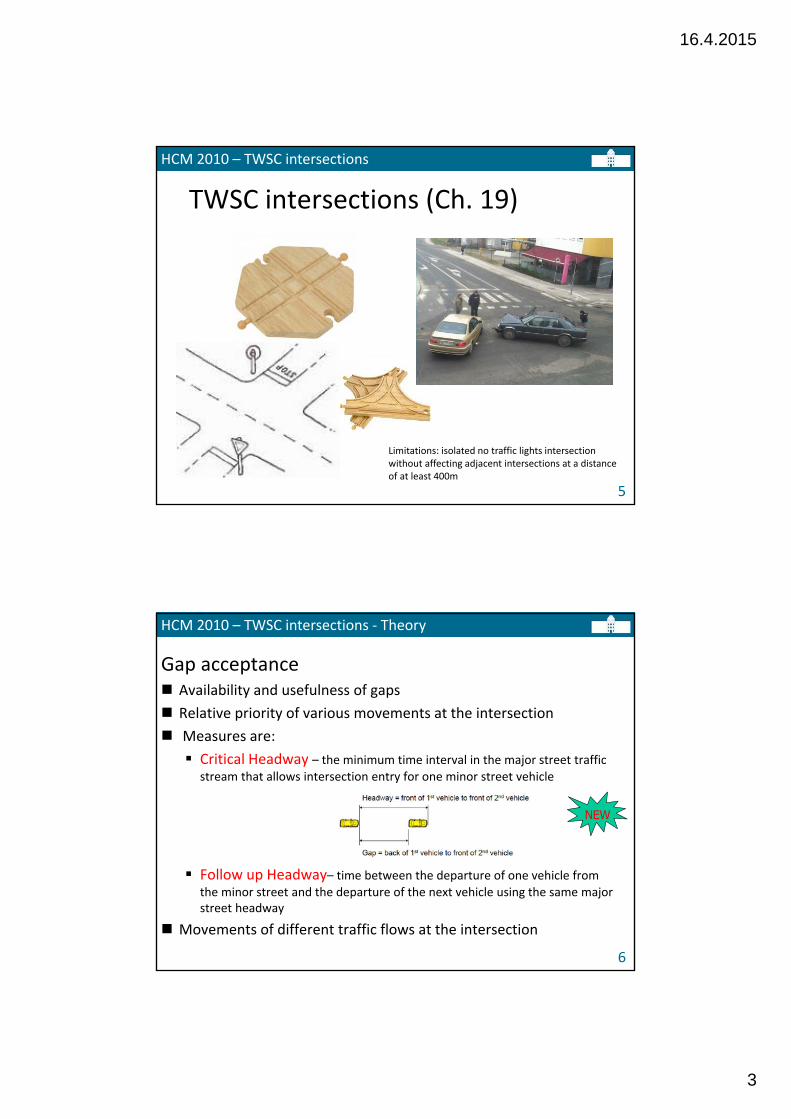
TWSC intersections (Ch. 19)
Limitations: isolated no traffic lights intersection without affecting adjacent intersections at a distance of at least 400m
HCM 2010 – TWSC intersections ‐ Theory
6
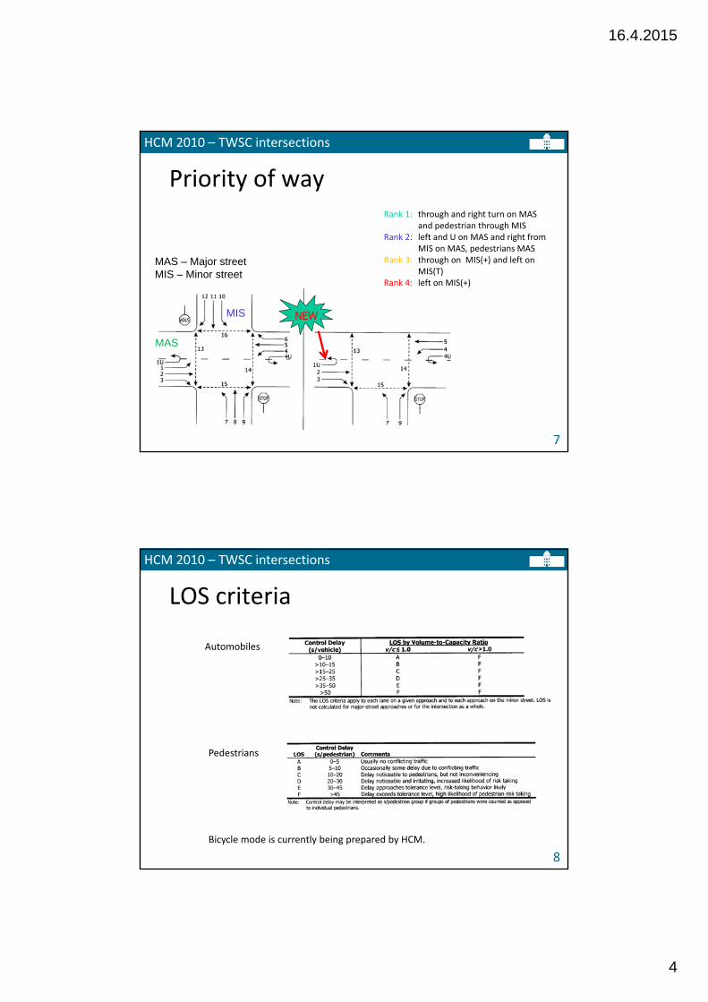
Gap acceptance Availability and usefulness of gaps
Relative priority of various movements at the intersection
Measures are:
Critical Headway – the minimum time interval in the major street traffic
stream that allows intersection entry for one minor street vehicle
Follow up Headway– time between the departure of one vehicle from
the minor street and the departure of the next vehicle using the same major street headway
Movements of different traffic flows at the intersection
NEW
16.4.2015
4
HCM 2010 – TWSC intersections
7
Priority of wayRank 1: through and right turn on MAS
and pedestrian through MISRank 2: left and U on MAS and right from
MIS on MAS, pedestrians MASRank 3: through on MIS(+) and left on
MIS(T)Rank 4: left on MIS(+)
MAS
MIS
MAS – Major streetMIS – Minor street
NEW
HCM 2010 – TWSC intersections
8
LOS criteria
Automobiles
Pedestrians
Bicycle mode is currently being prepared by HCM.
16.4.2015
5
HCM 2010 – TWSC intersections – Methodology (automobile)
9
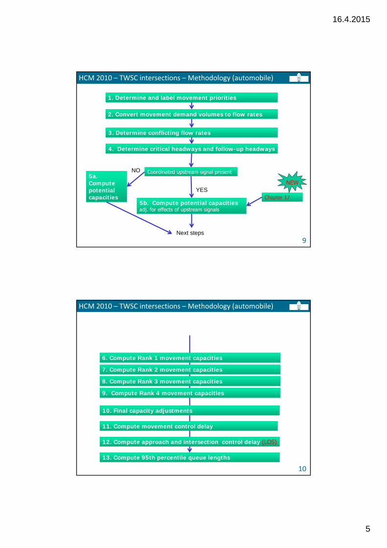
NO
YES
1. Determine and label movement priorities
2. Convert movement demand volumes to flow rates
3. Determine conflicting flow rates
4. Determine critical headways and follow-up headways
Coordinated upstream signal present
5b. Compute potential capacities adj. for effects of upstream signals
5a. Compute potential capacities Chapter 17
Next steps
NEW
HCM 2010 – TWSC intersections – Methodology (automobile)
10
9. Compute Rank 4 movement capacities
10. Final capacity adjustments
11. Compute movement control delay
12. Compute approach and intersection control delay (LOS)
13. Compute 95th percentile queue lengths
8. Compute Rank 3 movement capacities
7. Compute Rank 2 movement capacities
6. Compute Rank 1 movement capacities
16.4.2015
6
HCM 2010 – TWSC intersections
11
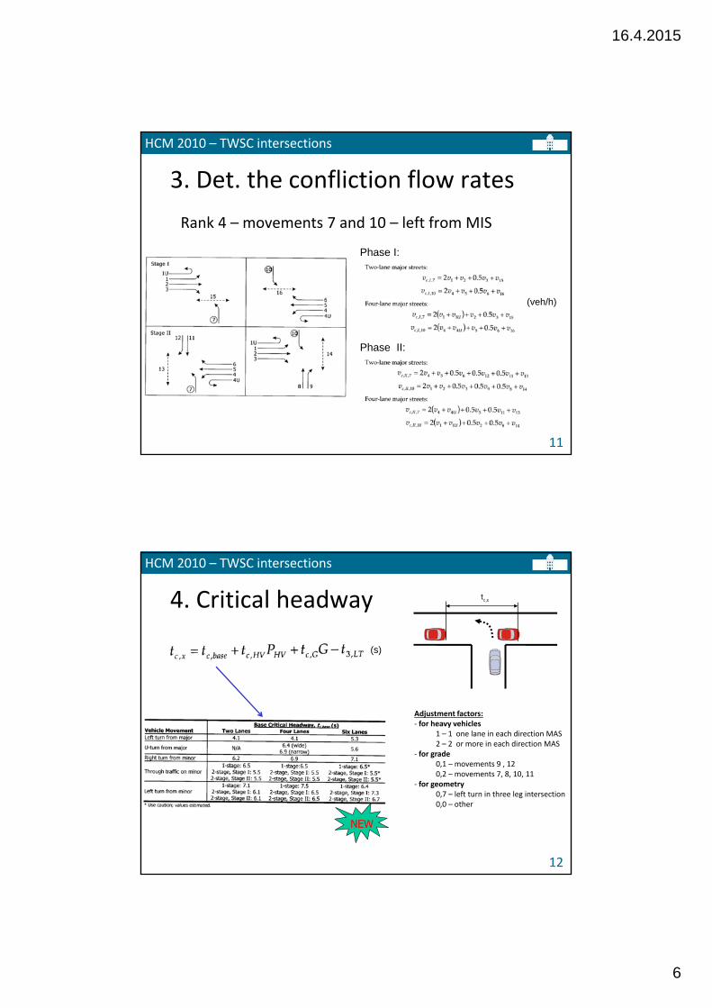
3. Det. the confliction flow rates
Rank 4 – movements 7 and 10 – left from MIS
Phase I:
Phase II:
(veh/h)
HCM 2010 – TWSC intersections
12
4. Critical headway x,ct
Adjustment factors:‐ for heavy vehicles
1 – 1 one lane in each direction MAS2 – 2 or more in each direction MAS
‐ for grade0,1 – movements 9 , 120,2 – movements 7, 8, 10, 11
‐ for geometry0,7 – left turn in three leg intersection0,0 – other
(s)
NEW
16.4.2015
7
HCM 2010 – TWSC intersections
13
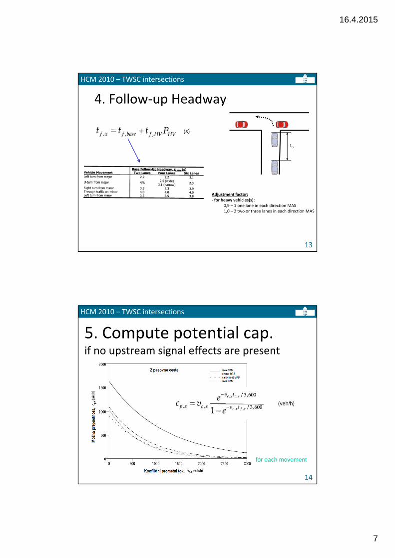
4. Follow‐up Headway
Adjustment factor:‐ for heavy vehicles(s):
0,9 – 1 one lane in each direction MAS1,0 – 2 two or three lanes in each direction MAS
(s)
x,ft
HCM 2010 – TWSC intersections
14
5. Compute potential cap.if no upstream signal effects are present
(veh/h)
for each movement
16.4.2015
8
(veh/h)
HCM 2010 – TWSC intersections
15
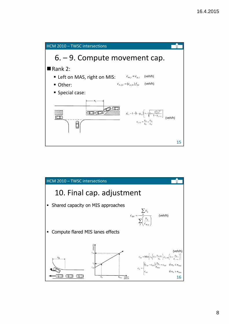
6. – 9. Compute movement cap.Rank 2: Left on MAS, right on MIS:
Other:
Special case:
(veh/h)
(veh/h)
HCM 2010 – TWSC intersections
16
10. Final cap. adjustment
Shared capacity on MIS approaches
Compute flared MIS lanes effects
(veh/h)
(veh/h)
16.4.2015
9
HCM 2010 – TWSC intersections
17
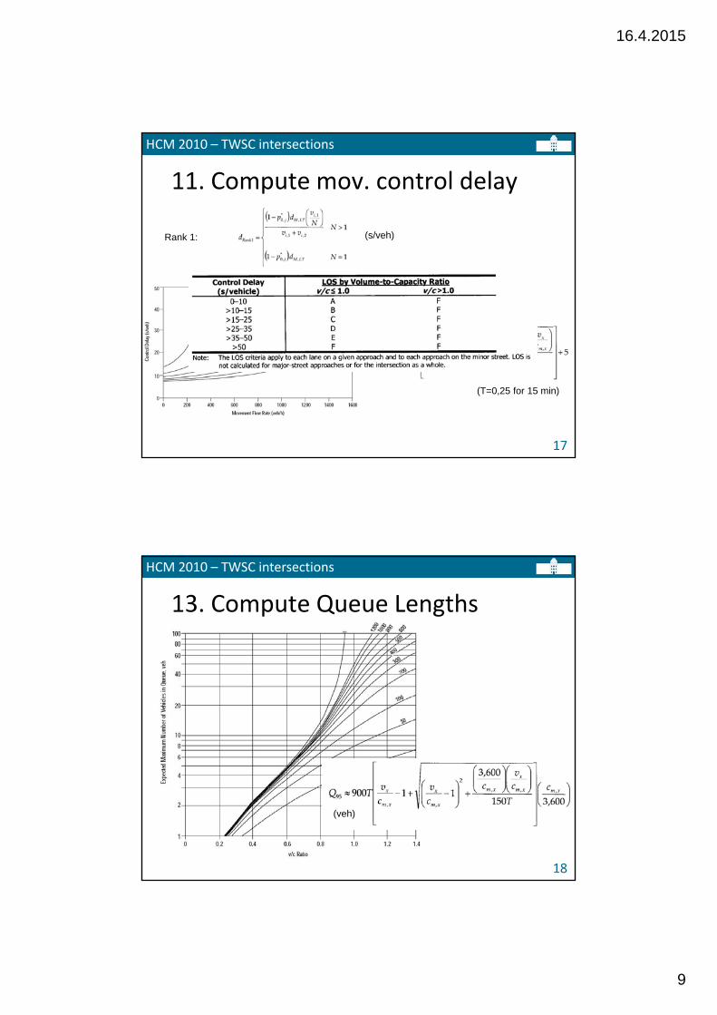
11. Compute mov. control delay
(T=0,25 for 15 min)
Rank 1:
Rank 2 – 4:
(s/veh)
HCM 2010 – TWSC intersections
18
13. Compute Queue Lengths
(veh)
16.4.2015
10
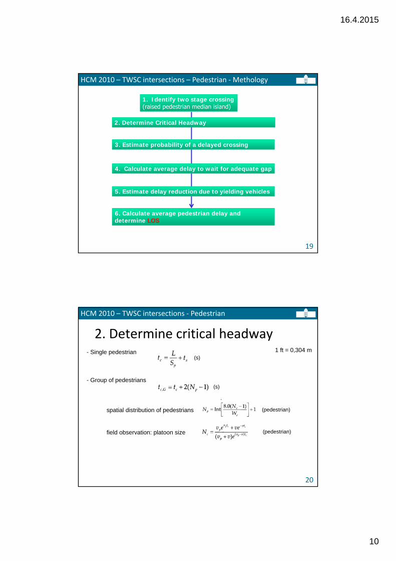
HCM 2010 – TWSC intersections – Pedestrian ‐Methology
19
1. Identify two stage crossing(raised pedestrian median island)
2. Determine Critical Headway
3. Estimate probability of a delayed crossing
4. Calculate average delay to wait for adequate gap
5. Estimate delay reduction due to yielding vehicles
6. Calculate average pedestrian delay and determine LOS
HCM 2010 – TWSC intersections ‐ Pedestrian
20
2. Determine critical headway1 ft = 0,304 m- Single pedestrian
(s)
- Group of pedestrians
spatial distribution of pedestrians (pedestrian)
field observation: platoon size
(s)
(pedestrian)

16.4.2015
11
HCM 2010 – TWSC intersections ‐ Pedestrian
21
3. Estimate prob. of delayed crossing
4. Calculate average delay
Probability of a blocked lane
Probability of a delayed crossing
(s)
Average pedestrian gap delay
No vehicle STOP
Average gap delay for pedestrian who incur nonzero delay
(s)
HCM 2010 – TWSC intersections ‐ Bicycles
22
No methodology specific to bicyclist has been developed
Bicyclist may travel either as a motor vehicle or a pedestrian
Critical headway distributions have been identified in the research for the bicycle crossing two lane MS
Multiple bicyclist often use the same gap in the vehicular traffic stream.

16.4.2015
12
Using HCS 2010
HCM 2010 ‐ Roundabouts
24
Roundabouts (Ch. 21)
Intersection with general circular shape, characterized by yield on entry and counter clockwise circulation around a central island.
16.4.2015
13
HCM 2010 – Roundabout – Theoretical basis
25
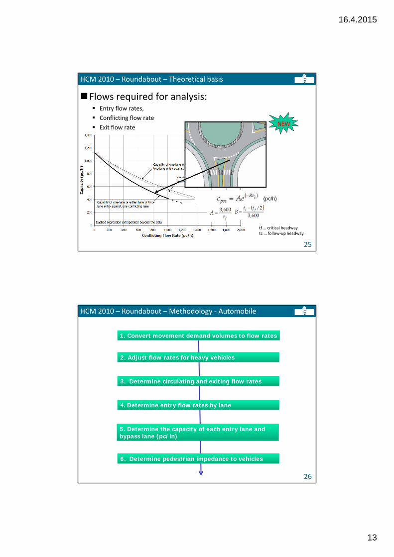
Flows required for analysis: Entry flow rates,
Conflicting flow rate
Exit flow rate
(pc/h)
tf … critical headwaytc … follow‐up headway
NEW
HCM 2010 – Roundabout – Methodology ‐ Automobile
26
1. Convert movement demand volumes to flow rates
2. Adjust flow rates for heavy vehicles
3. Determine circulating and exiting flow rates
5. Determine the capacity of each entry lane and bypass lane (pc/ln)
6. Determine pedestrian impedance to vehicles
4. Determine entry flow rates by lane
16.4.2015
14
HCM 2010 – Roundabout – Methodology ‐ Automobile
27
9. Compute the average control delay for each lane
10. Determine LOS for each lane on each approach
11. Compute control delay and determine LOS for each approach and the roundabout
12. Compute 95th percentile queues for each lane
8. Compute v/C ratio for each lane
7. Convert lane flow rates and capacities into veh/h
HCM 2010 – Roundabout
28
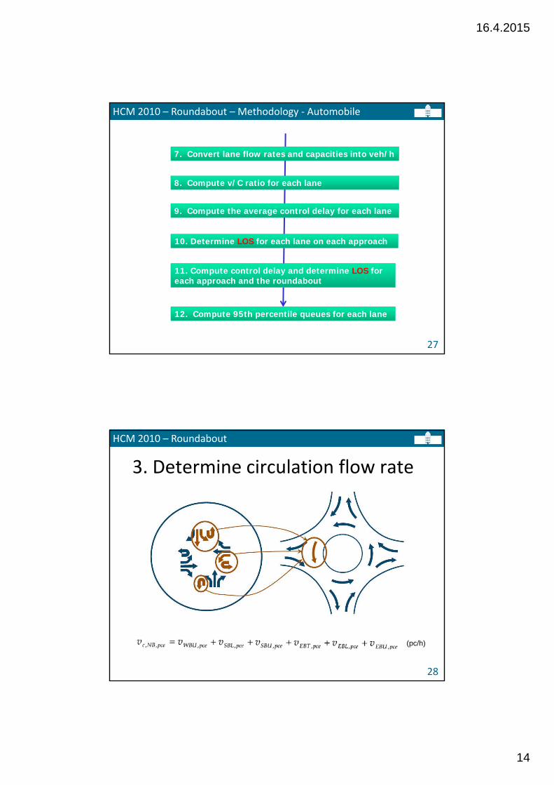
3. Determine circulation flow rate
(pc/h)
16.4.2015
15
HCM 2010 – Roundabout
29
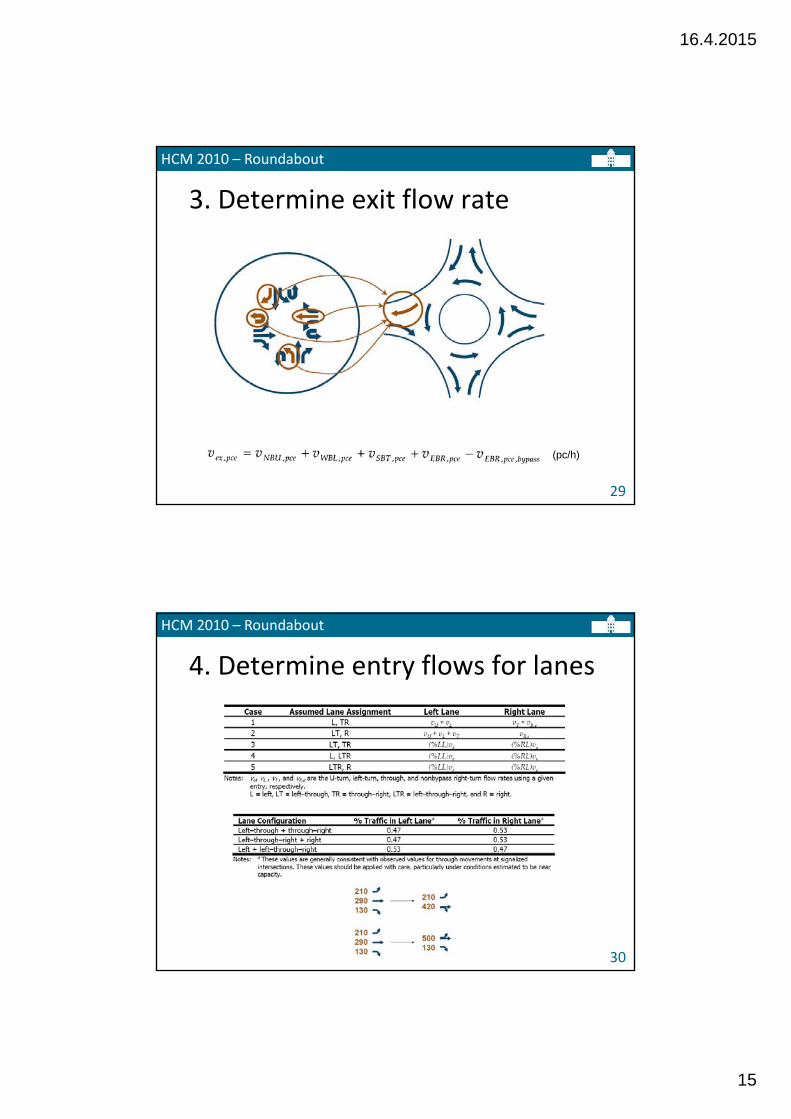
3. Determine exit flow rate
(pc/h)
HCM 2010 – Roundabout
30
4. Determine entry flows for lanes
16.4.2015
16
HCM 2010 – Roundabout – Theoretical basis
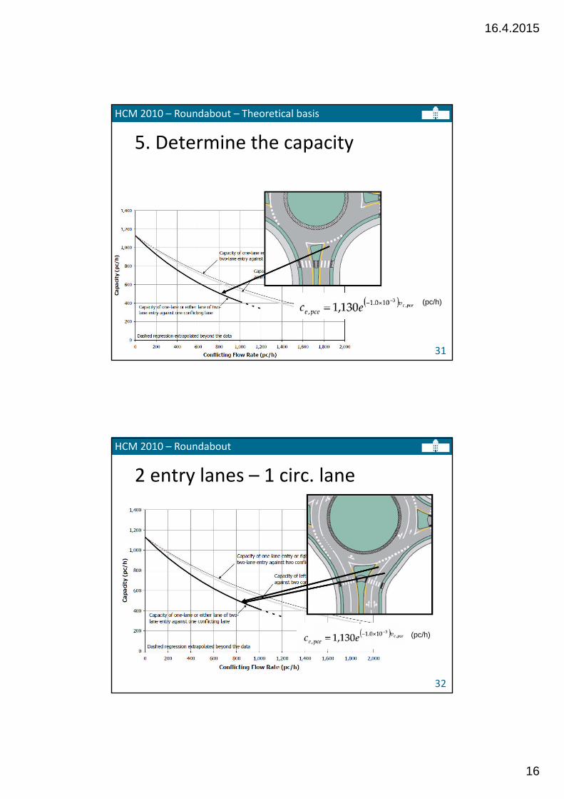
31
(pc/h)
5. Determine the capacity
HCM 2010 – Roundabout
32
2 entry lanes – 1 circ. lane
(pc/h)
16.4.2015
17
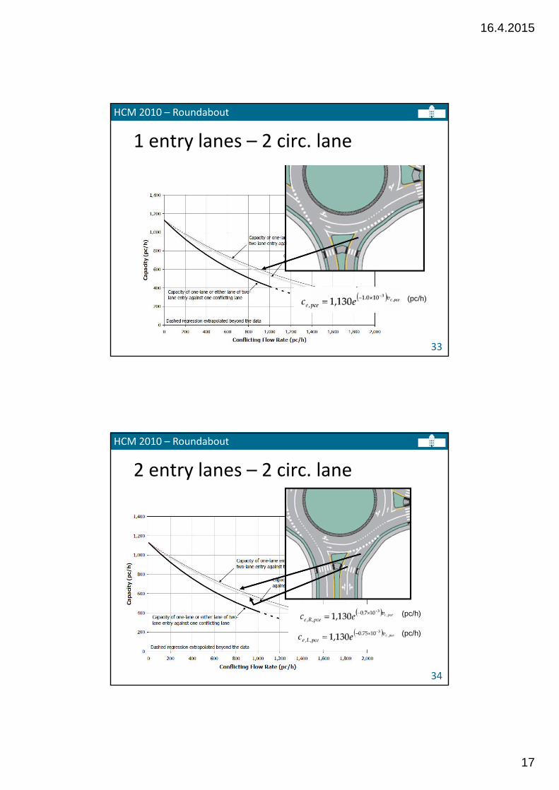
HCM 2010 – Roundabout
33
1 entry lanes – 2 circ. lane
(pc/h)
HCM 2010 – Roundabout
34
2 entry lanes – 2 circ. lane
(pc/h)
(pc/h)
16.4.2015
18
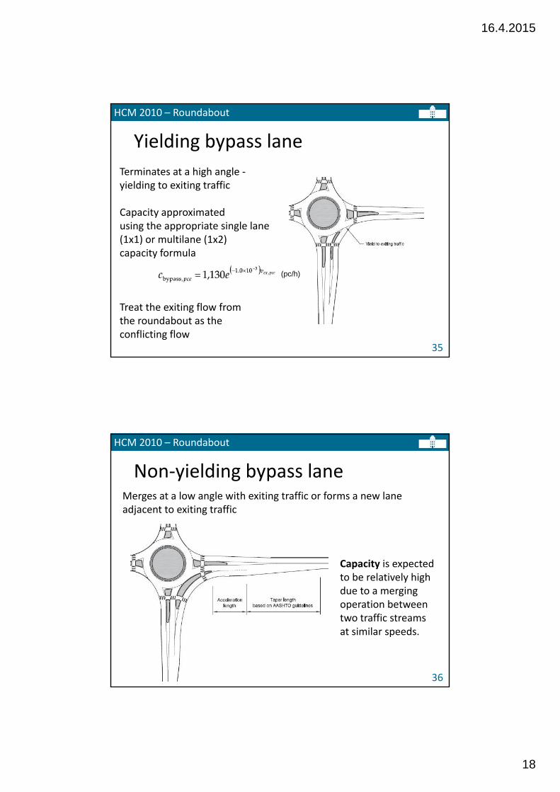
HCM 2010 – Roundabout
35
Yielding bypass lane
Terminates at a high angle ‐yielding to exiting traffic
Capacity approximatedusing the appropriate single lane(1x1) or multilane (1x2)capacity formula
Treat the exiting flow fromthe roundabout as theconflicting flow
(pc/h)
HCM 2010 – Roundabout
36
Non‐yielding bypass laneMerges at a low angle with exiting traffic or forms a new lane adjacent to exiting traffic
Capacity is expected to be relatively high due to a merging operation between two traffic streams at similar speeds.
16.4.2015
19
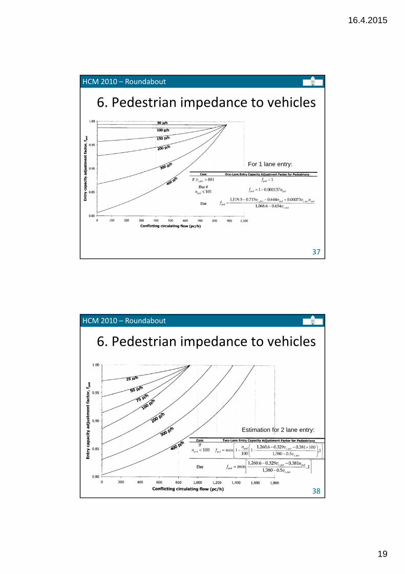
HCM 2010 – Roundabout
37
6. Pedestrian impedance to vehicles
For 1 lane entry:
HCM 2010 – Roundabout
38
6. Pedestrian impedance to vehicles
Estimation for 2 lane entry:
16.4.2015
20
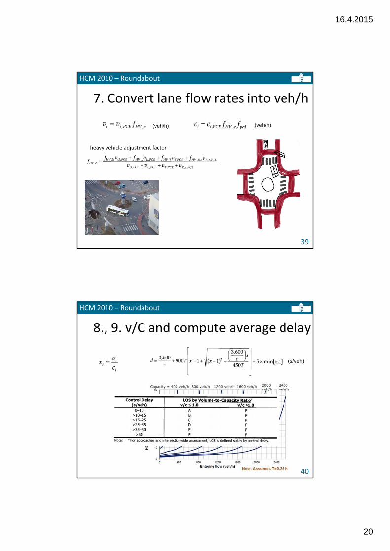
HCM 2010 – Roundabout
39
7. Convert lane flow rates into veh/h
(veh/h) (veh/h)
heavy vehicle adjustment factor
HCM 2010 – Roundabout
40
8., 9. v/C and compute average delay
(s/veh)
16.4.2015
21
HCM 2010 – Roundabout
41
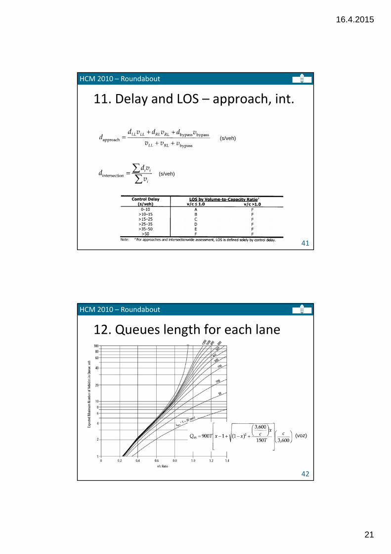
11. Delay and LOS – approach, int.
(s/veh)
(s/veh)
HCM 2010 – Roundabout
42
12. Queues length for each lane
(voz)
16.4.2015
22
HCM 2010 – Roundabout
43
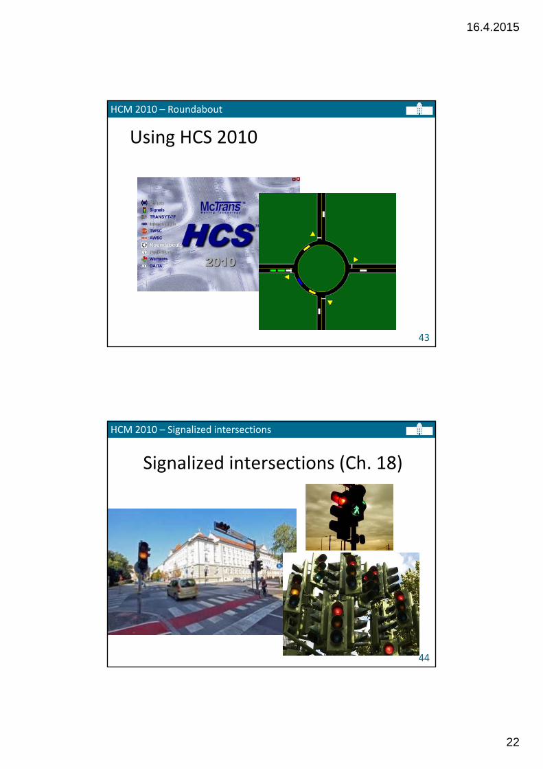
Using HCS 2010
HCM 2010 – Signalized intersections
44
Signalized intersections (Ch. 18)
16.4.2015
23
HCM 2010 – Signalized intersection – Theoretical basis
45
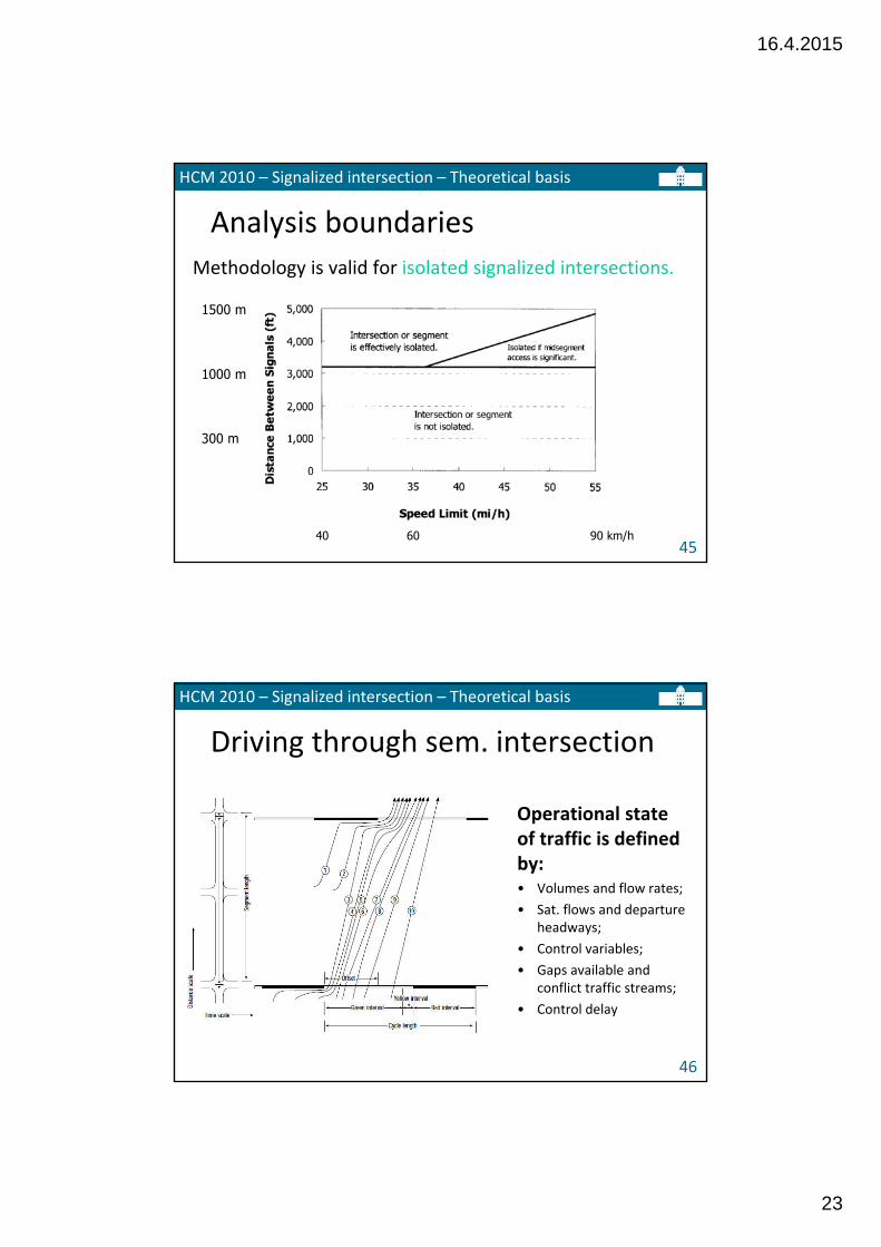
Analysis boundaries
1500 m
1000 m
300 m
40 60 90 km/h
Methodology is valid for isolated signalized intersections.
HCM 2010 – Signalized intersection – Theoretical basis
46
Driving through sem. intersection
Operational state of traffic is defined by:• Volumes and flow rates;
• Sat. flows and departure headways;
• Control variables;
• Gaps available and conflict traffic streams;
• Control delay
16.4.2015
24
HCM 2010 – Signalized intersection – Theoretical basis
47
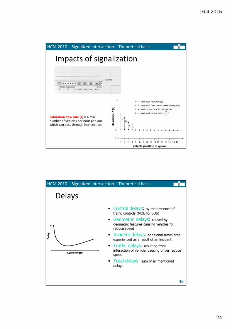
Impacts of signalization
Saturation flow rate (s) is a max. number of vehicles per hour per lane, which can pass through intersection.
HCM 2010 – Signalized intersection – Theoretical basis
48
Delays
• Control delays: by the presence of traffic controls (MOE for LOS)
• Geometric delays: caused by geometric features causing vehicles for reduce speed
• Incident delays: additional travel time experienced as a result of an incident
• Traffic delays: resulting from interaction of vehicle, causing driver reduce speed
• Total delays: sum of all mentioned delays
16.4.2015
25
HCM 2010 – Signalized intersection – Theoretical basis
49
What is new in HCM 2010
1. The model has been set up to handle actuated signal analysis directly.
2. The estimation of delay is partially modeled using Incremental Queue Analysis (IQA) which allows a more detailed analysis of arriving and departing vehicle distributions.
3. The definition of lane groups has been altered. Lane groups are identified and separately analyzed.
“This presentation focuses on the analysis of pretimed signals because it is more straight forward to present basic modeling theory for fixed time signals.”
HCM 2010 – Signalized intersection – Theoretical basis
50
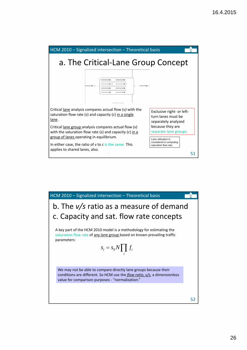
Conceptual framework
Five fundamental concepts:
The critical lane group concept
The v/s ratio as a measure of demand
Capacity and saturation flow rate concepts
Level‐of‐service (LOS) criteria and concepts
Effective green time and lost‐time concepts
16.4.2015
26
HCM 2010 – Signalized intersection – Theoretical basis
51
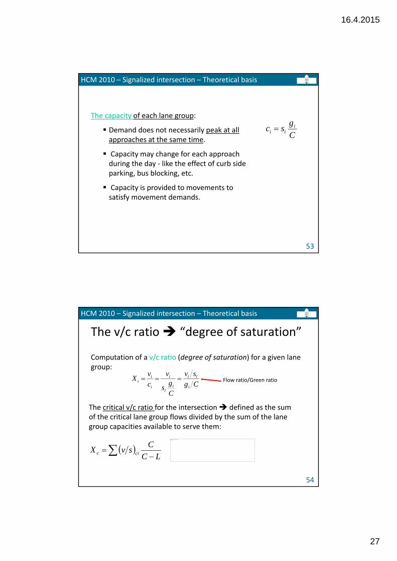
a. The Critical‐Lane Group Concept
Chapter 24
Critical lane analysis compares actual flow (v) with the saturation flow rate (s) and capacity (c) in a single lane.
Critical lane group analysis compares actual flow (v) with the saturation flow rate (s) and capacity (c) in a group of lanes operating in equilibrium.
In either case, the ratio of v to c is the same. This applies to shared lanes, also.
Exclusive right‐ or left‐turn lanes must be separately analyzed because they are separate lane groups.
Lane utilization is considered in computing saturation flow rate.
HCM 2010 – Signalized intersection – Theoretical basis
52
b. The v/s ratio as a measure of demand c. Capacity and sat. flow rate concepts
A key part of the HCM 2010 model is a methodology for estimating the saturation flow rate of any lane group based on known prevailing traffic parameters:
i
ii fNss 0
We may not be able to compare directly lane groups because their conditions are different. So HCM use the flow ratio, v/s, a dimensionless value for comparison purposes ‐ “normalization.”
16.4.2015
27
HCM 2010 – Signalized intersection – Theoretical basis
53
The capacity of each lane group:
Demand does not necessarily peak at all approaches at the same time.
Capacity may change for each approach during the day ‐ like the effect of curb side parking, bus blocking, etc.
Capacity is provided to movements to satisfy movement demands.
C
gsc i
ii
HCM 2010 – Signalized intersection – Theoretical basis
54
The v/c ratio “degree of saturation”
Computation of a v/c ratio (degree of saturation) for a given lane group:
Cg
sv
Cg
s
v
c
vX
i
ii
ii
i
i
ii Flow ratio/Green ratio
The critical v/c ratio for the intersection defined as the sum of the critical lane group flows divided by the sum of the lane group capacities available to serve them:
LC
CsvX cic
Slike trenutno ni mogoče prikazati.
16.4.2015
28
HCM 2010 – Signalized intersection – Theoretical basis
55
Computation of a v/c ratio for an intersection as a whole:
If the critical v/c ratio is less than 1.00, the cycle length, phase plan, and physical design provided are sufficient to handle the demand and flows specified.
But, having a critical v/c ratio under 1.00 does not assure that every critical lane group has v/c ratios under 1.00. When the critical v/c ratio is less than 1.00, but one or more lane groups have v/c rations greater than 1.00, the green time has been misallocated.
If the Xc > 1.0, then the physical design, phase plan, and cycle length specified do not provide sufficient capacity for the anticipated or existing critical lane group flows. Do something to increase capacity:
(1) longer cycle lengths (less number of cycles, less lost time),
(2) better phase plans (improved LT treatment), and
(3) add critical lane group or groups (meaning change approach layouts increase capacity)
HCM 2010 – Signalized intersection – Theoretical basis
56
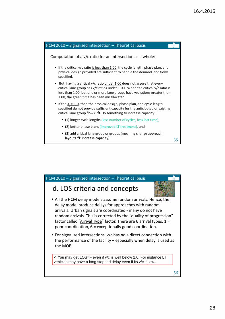
d. LOS criteria and concepts
All the HCM delay models assume random arrivals. Hence, the delay model produce delays for approaches with random arrivals. Urban signals are coordinated ‐many do not have random arrivals. This is corrected by the “quality of progression” factor called “Arrival Type” factor. There are 6 arrival types: 1 = poor coordination, 6 = exceptionally good coordination.
For signalized intersections, v/c has no a direct connection with the performance of the facility – especially when delay is used as the MOE.
You may get LOS=F even if v/c is well below 1.0. For instance LT vehicles may have a long stopped delay even if its v/c is low..
16.4.2015
29
HCM 2010 – Signalized intersection – Theoretical basis
57
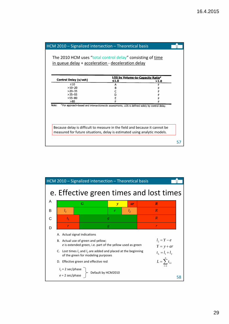
The 2010 HCM uses “total control delay” consisting of time in queue delay + acceleration ‐ deceleration delay
Because delay is difficult to measure in the field and because it cannot be measured for future situations, delay is estimated using analytic models.
HCM 2010 – Signalized intersection – Theoretical basis
58
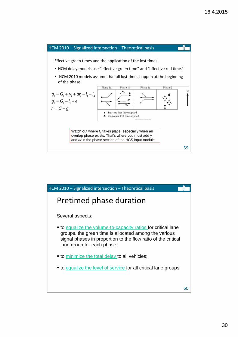
e. Effective green times and lost timesG y ar R
l1 e l2 R
tL g R
r g r
A
B
C
DA. Actual signal indications
B. Actual use of green and yellow; e is extended green, i.e. part of the yellow used as green
C. Lost times l1 and l2 are added and placed at the beginning of the green for modeling purposes
D. Effective green and effective red
l1 = 2 sec/phase
e = 2 sec/phase
n
iLi
L
tL
llt
aryY
eYl
1
21
2
Default by HCM2010
16.4.2015
30
HCM 2010 – Signalized intersection – Theoretical basis
59
Effective green times and the application of the lost times:
HCM delay models use “effective green time” and “effective red time.”
HCM 2010 models assume that all lost times happen at the beginning of the phase.
ii
ii
iiii
gCr
elGg
llaryGg
1
21
Watch out where tL takes place, especially when an overlap phase exists. That’s where you must add yand ar in the phase section of the HCS input module.
HCM 2010 – Signalized intersection – Theoretical basis
60
Pretimed phase duration
Several aspects:
to equalize the volume‐to‐capacity ratios for critical lane groups. the green time is allocated among the various signal phases in proportion to the flow ratio of the critical lane group for each phase;
to minimize the total delay to all vehicles;
to equalize the level of service for all critical lane groups.
16.4.2015
31
HCM 2010 – Signalized intersection – Theoretical basis
61
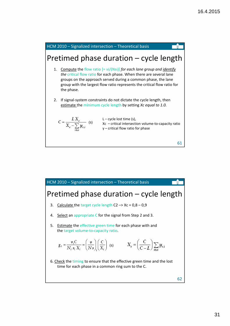
Pretimed phase duration – cycle length1. Compute the flow ratio [= vi/(Nsi)] for each lane group and identify
the critical flow ratio for each phase. When there are several lane groups on the approach served during a common phase, the lane group with the largest flow ratio represents the critical flow ratio for the phase.
2. If signal‐system constraints do not dictate the cycle length, then estimate the minimum cycle length by setting Xc equal to 1.0.
L – cycle lost time (s),Xc – critical intersection volume‐to‐capacity ratioy – critical flow ratio for phase
(s)
3. Calculate the target cycle length C2 –> Xc = 0,8 – 0,9
4. Select an appropriate C for the signal from Step 2 and 3.
5. Estimate the effective green time for each phase with andthe target volume‐to‐capacity ratio.
6. Check the timing to ensure that the effective green time and the lost time for each phase in a common ring sum to the C.
HCM 2010 – Signalized intersection – Theoretical basis
62
Pretimed phase duration – cycle length
(s)
16.4.2015
32
HCM 2010 – Signalized intersection – Methodology (automobile)
63
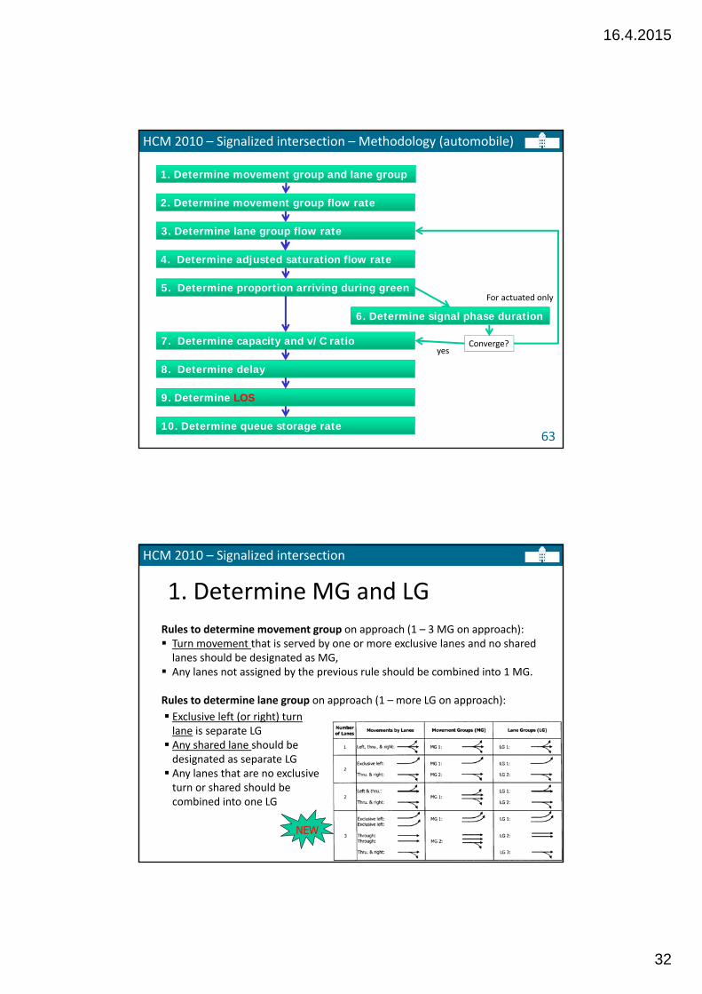
1. Determine movement group and lane group
2. Determine movement group flow rate
3. Determine lane group flow rate
4. Determine adjusted saturation flow rate
10. Determine queue storage rate
5. Determine proportion arriving during green
8. Determine delay
7. Determine capacity and v/C ratio
6. Determine signal phase duration
9. Determine LOS
For actuated only
Converge?yes
HCM 2010 – Signalized intersection
64
1. Determine MG and LG
Rules to determine movement group on approach (1 – 3 MG on approach): Turn movement that is served by one or more exclusive lanes and no shared lanes should be designated as MG,
Any lanes not assigned by the previous rule should be combined into 1 MG.
Rules to determine lane group on approach (1 – more LG on approach):
Exclusive left (or right) turn lane is separate LG Any shared lane should be designated as separate LG Any lanes that are no exclusive turn or shared should be combined into one LG
NEW
16.4.2015
33
HCM 2010 – Signalized intersection
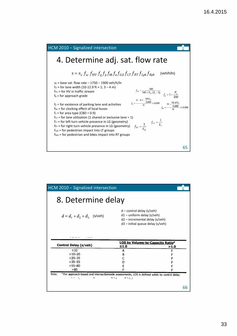
65
4. Determine adj. sat. flow rate
(veh/h/ln)
s0 = base sat. flow rate – 1750 – 1900 veh/h/lnfw = for lane width (10‐12.9 ft = 1; 3 – 4 m)fHV = for HV in traffic stream fg = for approach grade
fp = for existence of parking lane and activitiesfbb = for clocking effect of local busesfa = for area type (CBD = 0.9)fLU = for lane utilization (1 shared or exclusive lane = 1)fLT = for left turn vehicle presence in LG (geometry)fRT = for right turn vehicle presence in LG (geometry)fLpb = for pedestrian impact into LT groupsfRpb = for pedestrian and bikes impact into RT groups
HCM 2010 – Signalized intersection
66
8. Determine delay
(s/veh)
d – control delay (s/veh)d1 – uniform delay (s/veh)d2 – incremental delay (s/veh)d3 – initial queue delay (s/veh)
(s/veh)
(s/veh)
(s/veh)
16.4.2015
34
HCM 2010 – Signalized intersection ‐ Pedestrian
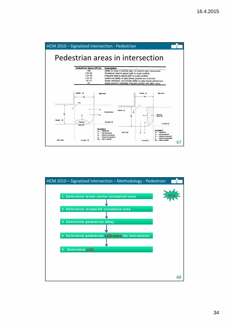
67
Pedestrian areas in intersection
>5,6>3,7-5,6>2,3-3,7>1,4-2,3>0,8-1,4<0,8
HCM 2010 – Signalized intersection – Methodology ‐ Pedestrian
68
1. Determine street corner circulation area
2. Determine crosswalk circulation area
3. Determine pedestrian delay
4. Determine pedestrian LOS score for intersection
5. Determine LOS
NEW
16.4.2015
35
HCM 2010 – Signalized intersection ‐ Pedestrian
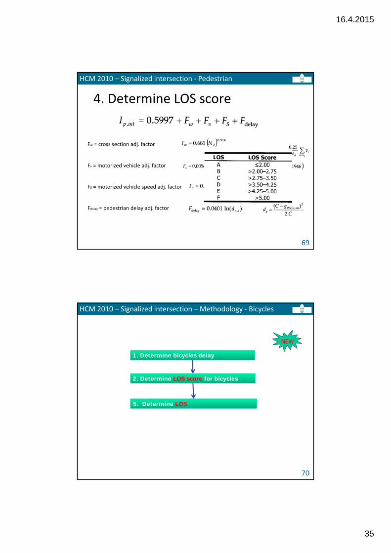
69
4. Determine LOS score
Fw = cross section adj. factor
Fv = motorized vehicle adj. factor
FS = motorized vehicle speed adj. factor
Fdelay = pedestrian delay adj. factor
HCM 2010 – Signalized intersection – Methodology ‐ Bicycles
70
1. Determine bicycles delay
2. Determine LOS score for bicycles
5. Determine LOS
NEW
16.4.2015
36
HCM 2010 – Signalized intersection ‐ Bicycles
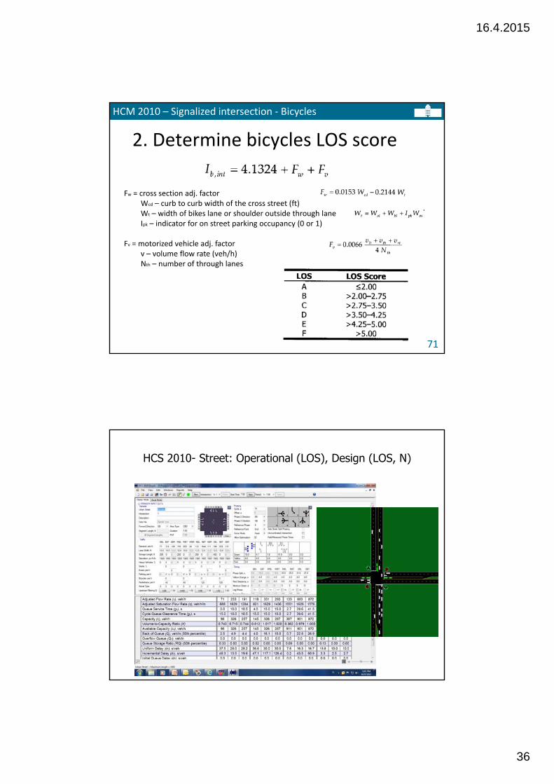
71
2. Determine bicycles LOS score
Fw = cross section adj. factorWcd – curb to curb width of the cross street (ft)Wt – width of bikes lane or shoulder outside through laneIpk – indicator for on street parking occupancy (0 or 1)
Fv = motorized vehicle adj. factorv – volume flow rate (veh/h)Nth – number of through lanes
HCS 2010- Street: Operational (LOS), Design (LOS, N)


![Traffic Flow Control - Home Page | Kent State …dragan/ST-Spring2016/Traffic Flow...Traffic Flow and Circular-arc Graph, PPT, AbdulhakeemMohammed, [2007]Recognition of Circular-Arc](https://static.fdocuments.net/doc/165x107/5eca5f06bc8dcc00d54c2eea/traffic-flow-control-home-page-kent-state-draganst-spring2016traffic-flow.jpg)