4-Component Relativistic Calculations in

Solution with the Polarizable Continuum Model

of Solvation: Theory, Implementation and

Application to the Group 16 Dihydrides H2X (X

= O, S, Se, Te, Po)

Roberto Di Remigio,∗,†,‖ Radovan Bast,‡,¶,⊥ Luca Frediani,† and Trond Saue∗,§

Department of Chemistry, Centre for Theoretical and Computational Chemistry, University

of Tromsø, N-9037 Tromsø, Norway, Department of Theoretical Chemistry and Biology,

School of Biotechnology, Royal Institute of Technology, AlbaNova University Center,

S-10691 Stockholm, Sweden, PDC Center for High Performance Computing, Royal

Institute of Technology, S-10044 Stockholm, Sweden, and Laboratoire de Chimie et

Physique Quantiques (UMR 5626) CNRS/Universite de Toulouse 3 (Paul Sabatier) 118

route de Narbonne, 31062 Toulouse, France

E-mail: roberto.d.remigio@uit.no; trond.saue@irsamc.ups-tlse.fr

1

Abstract

We present a formulation of 4-component relativistic self-consistent field (SCF) the-

ory for a molecular solute described within the framework of the polarizable continuum

model (PCM) for solvation. The linear response function for a 4-component PCM-SCF

state is also derived, as well as the explicit form of the additional contributions to

the first-order response equations. The implementation of such a 4-component PCM-

SCF model, as carried out in a development version of the DIRAC program package,

is documented. In particular, we present the newly developed application program-

ming interface (API) PCMSolver used in the actual implementation with DIRAC. To

demonstrate the applicability of the approach we present and analyze calculations of

solvation effects on the geometries, electric dipole moments and static electric dipole

polarizabilities for the group 16 dihydrides H2X (X = O, S, Se, Te, Po).

Keywords

Continuum solvation, relativistic quantum chemistry, electrostatic potential, modular pro-

gramming, linear response, polarizability, dipole moment

∗To whom correspondence should be addressed†Department of Chemistry, Centre for Theoretical and Computational Chemistry, University of Tromsø,

N-9037 Tromsø, Norway‡Department of Theoretical Chemistry and Biology, School of Biotechnology, Royal Institute of Technol-

ogy, AlbaNova University Center, S-10691 Stockholm, Sweden¶PDC Center for High Performance Computing, Royal Institute of Technology, S-10044 Stockholm, Swe-

den§Laboratoire de Chimie et Physique Quantiques (UMR 5626) CNRS/Universite de Toulouse 3 (Paul

Sabatier) 118 route de Narbonne, 31062 Toulouse, France‖Previous address: Dipartimento di Chimica e Chimica Industriale, Universita di Pisa, via Risorgimento

35, 56126 Pisa, Italy⊥Previous address: Laboratoire de Chimie et Physique Quantiques (UMR 5626) CNRS/Universite de

Toulouse 3 (Paul Sabatier) 118 route de Narbonne, 31062 Toulouse, France

2

1 Introduction

Paul Adrien Maurice Dirac, who developed the relativistic wave equation for the electron,

stated that relativistic effects would be of “no importance in the consideration of atomic and

molecular structure and ordinary chemical reactions”1. Trusting Dirac’s words, most of the

successful development in quantum chemistry has been based on nonrelativistic quantum

mechanics, but Dirac’s statement has been proven incorrect2. From a chemist’s point of

view, this is not obvious. Relativistic corrections depend on the ratio between particle speed

and the speed of light3. Since valence electrons have small kinetic energies, one would

think, as did Dirac, that chemical bonding and structure would be unaffected. After all,

most chemical phenomena take place at energies well below the relativistic regime: the rest

energy of an electron (mec2) is half a mega-electron volt, while most chemical processes occur

on an energy scale of few electronvolts.

This is not entirely true: it soon became clear in the history of theoretical chemistry, that

a nonrelativistic theory could not explain certain trends in observed properties. As recently

reviewed by Pyykko, relativistic effects play a prominent role, especially in inorganic chem-

istry4. Periodic trends, such as the increase in atomic dimensions and ionization potentials,

may be broken for the heaviest elements of the Periodic Table. Many examples are known,

the most well-known maybe being the relativistic origin of the color of gold5.

In a less known part of his famous quote,1 Dirac advocates the development of numerical

methods to solve the Schrodinger’s equation. Although this effort has largely been under-

taken for isolated molecules, the presence of solvent still poses a formidable challenge. On

the other hand, the ability to account, at least qualitatively, for environment effects is funda-

mental in all experimental branches of chemistry: structures, energies and reaction barriers,

as well as spectroscopic observables, are greatly influenced by environment effects. Despite

the large number of reactions known to happen in the solid state and in gas phase, we can

safely state that most chemistry happens in solution6. The theoretical treatment of envi-

ronment effects suffers from a dimensionality problem: even the most simplified picture of

3

the system under consideration would require taking into account 500–1000 atoms, at least.

Direct application of quantum chemistry methods is therefore impossible and not even desir-

able for such systems. In problems with a high dimensionality, the microscopic detail in the

physical description cannot account for the macroscopic behavior of the system7–9. Models

must be devised to overcome the dimensionality “disease”.

It is customary to divide the models proposed into two broad classes, according to the

microscopic description of the solvent these models give. Continuum (or implicit) models,

deal explicitly only with the degrees of freedom associated with the solute, while replacing

the solvent with a structureless continuum characterized by its bulk properties10,11. Discrete

(or explicit) models, treat degrees of freedom associated with the solvent molecules and the

solute explicitly. The two sets of coordinates can be treated at different levels of theory.

The quantum mechanics/molecular mechanics (QM/MM) family of methods is a notable

example12–14. QM/MM and continuum methods can also be combined15–17, to achieve a

faithful, yet cost-effective strategy to reproduce solvent effects.

It is very well recognized that both solvent and relativistic effects can play an important

role in the chemistry of heavy-element containing species. The field of actinide chemistry

is in this respect a notable example18. Computational actinide chemistry is a very active

field19,20 and proper treatment of relativistic and solvent effects is mandatory: gaining insight

about actinide species from experiment can be rather difficult or not practicable due to the

safety and security hazards their radioactivity poses.

Relativistic and solvent effects also play an important role in the accurate prediction of

NMR parameters of heavy-element containing species. Chemical shifts and indirect spin–

spin coupling constants show great sensitivity to the chemical environment of the probe

nucleus21. Such observables are excellent benchmarks for assessing the accuracy of compu-

tational models for the inclusion of relativistic and solvent effects.

Despite numerous studies in the literature22–24, a black-box strategy for the inclusion of

both relativistic and solvent effects in a manner that is both efficient and accurate is not

4

yet available. Many applications in the calculation of structures and energetics of heavy-

element containing species make use of effective core potentials (ECPs) in a DFT or wave

function theory framework25–32. In other studies, the more refined Zeroth-Order Regular

Approximation (ZORA) Hamiltonian33 has been used, either in the scalar, spin-free form or

in a 2-component framework, including spin-orbit effects34–39. The second-order Douglas–

Kroll–Hess (DKH2) in spin-free form, has also been applied40. In the above cited studies

continuum approaches, notably the conductor-like screening model (COSMO)41–43, have

been adopted for the inclusion of solvent effects, in many cases complementing a cluster

approach, treating the first solvation shell explicitly at the same level of theory as the solute.

QM/MM studies on uranium complexes in water solution44,45 and copper in plastocyanins46

have also appeared. Chaumont and Wipff47 presented a study of uranyl and europium

solvation in room-temperature ionic liquids based on MD simulations combined with QM

calculations on selected snapshots.

The calculation of NMR parameters for heavy-element containing compounds covers a

large part of the existing literature. Autschbach and co-workers have presented extensive

studies of shieldings and couplings for Pt−Tl, Pt and Hg containing species, alternatively

using the cluster48,49 and cluster/continuum50–54 approaches. In other studies of indirect

spin–spin coupling constants by the same group55,56, Born–Oppenheimer molecular dynamics

(BOMD) simulations were used to account for specific solvent effects.

In all aforementioned studies, bulk solvent effects, described by use of a continuum model

such as COSMO, were found to be extremely important in order to achieve a qualitatively

accurate description of the phenomena of interest. Remarkably, such a conclusion was

reached for aprotic23 and protic50,54 solvents alike. However, a purely continuum description

might in some cases not be adequate, to capture all relevant solute-solvent effects, requir-

ing a cluster/continuum26,35,50,52, QM/MM44–46 or ab initio molecular dynamics (AIMD)

approach54–58.

All the studies currently available in the literature emphasize the importance of both rela-

5

tivistic and solvent effects. However, with the exception of a recent frozen density embedding

subsystem approach? ? , a scheme whereby the 4-component Dirac–Coulomb Hamiltonian

is coupled to an environment is not yet available. In the present contribution we report the

interfacing of the polarizable continuum model (PCM)59, a continuum solvation model, with

a 4-component relativistic description of the solute. The equations derived are based on the

self-consistent field (SCF) approximation for the wave function, either Hartree–Fock (HF)

or Kohn–Sham density-functional theory (KS-DFT). The linear response (LR) function for

the calculation of static second-order properties is also derived. We furthermore present a

working implementation, making use of a modular programming paradigm (vide infra).

Due to the theoretical similarity between the PCM, more refined polarizable molecu-

lar mechanics13,14 and even three-layer methodologies15–17, this work constitutes a starting

point for more accurate models for the inclusiont of environment effects in computational

procedures based on relativistic Hamiltonians.

The remainder of the paper is organized as follows. In Section 2, a detailed presentation

of the theory underlying the 4-component implementation of the PCM-SCF and LR-PCM-

SCF algorithms is presented. In Section 3, our modular approach to the implementation

in the DIRAC program60 is discussed, with particular emphasis on the recently developed

PCMSolver application programming interface (API)61. As a first application, we present in

Section 4 geometries and electric properties of the group 16 dihydrides, with and without

solvent effects included. Conclusions and perspectives for this work are presented in Section

5. SI-based atomic units62 will be employed throughout the paper ( = me = e = 14πε0

= 1),

electron mass and charge will however be always specified explicitly in the equations. We

will denote the identity matrix in a N -dimensional space by IN .

6

2 Theory

Sections 2.1 and 2.2 briefly summarize 4-component Hamiltonians and the IEF-PCM for-

malism, respectively. These are our points of departure for the formulation of the coupling

of a 4-component description of the solute with a continuum solvation model, presented in

Sections 2.3 and 2.4.

2.1 4-component Hamiltonians

As recently emphasized by Saue63, the molecular electronic Hamiltonian may be written in

the general form:

H0 =N∑i

h(ri) +1

2

N∑i,j=1

g(ri, rj) + VNN. (1)

i. e. as the sum of one- and two-electron parts together with a scalar shift VNN due to the

classical repulsion of clamped nuclei in the Born-Oppenheimer approximation. This general

form remains valid whether relativity is being considered or not. Much alike the concept

of nonrelativistic model chemistries one can consider relativity as the third dimension of

quantum chemistry. The actual Hamiltonian model and the corresponding “rung” in the

hierarchy of relativistic model chemistries is completely specified once the one- and two-

electron operators have been fixed.

In 4-component relativistic quantum chemistry, the one-electron Hamiltonian is taken

to be the Dirac one-electron Hamiltonian3,64. In the field of the clamped nuclei and in the

absence of any other external field, we have:

hD =

VNeI2 c(σ · p)

c(σ · p) (VNe − 2mec2)I2

; VNe = −e∑A

∫dr′

ρA(r′)

|r − r′|(2)

where c is the speed of light. The nuclear charge distributions may be chosen to have a

finite spatial extent, as apparent from the above definition of the clamped-nuclei attractive

potential. Furthermore notice that the form of VNe is the same as in nonrelativistic theory,

7

but its physical content in the relativistic context is markedly different, in that it also contains

the spin-orbit interaction63. Finally, σ is a vector containing the Pauli spin matrices3.

In the relativistic context, the formulation of the two-electron interaction requires careful

consideration. The full history of the interacting particles is required for a complete de-

scription of the two-electron interaction, and no closed expression is available for use in the

electronic Hamiltonian. Rather, a perturbation expansion of the full two-electron interaction

in orders of c−2 can be used3

g(r1, r2) ' gC(r1, r2) + gG(r1, r2) + ggauge(r1, r2)

=I4 · I4

r12

− cα1 · cα2

c2r12

− (cα1 · r12)(cα2 · r12)

c2r312

(3)

While the Coulomb term gC represents the well-known charge-charge interaction, the Gaunt

term gG introduces a current-current interaction. A Foldy–Wouthuysen transformation65

achieves reduction to 2-component form unveiling the physical content of these terms66,67.

The Coulomb and Gaunt terms give rise to spin-orbit interaction of spin-same-orbit and

spin-other-orbit type, respectively. The Gaunt term also carries the full spin-spin interaction,

whereas the gauge-dependent term ggauge of Eq. (3) must be included for the full orbit-orbit

interaction.

Different Hamiltonians to be used in relativistic molecular electronic-structure theory

are built from the one-electron part in Eq. (2) and the two-electron interaction in Eq. (3),

truncated at a suitable order in c−2. Keeping only the Coulomb term gives rise to the

Dirac–Coulomb (DC) Hamiltonian for an N -electron system:

HDC =N∑i=1

hD(ri) +1

2

N∑i,j=1

gC(ri, rj) (4)

It must be pointed out that the one-electron Hamiltonian in Eq. (2) is unbounded from

below, so that one might expect that building a variational theory on it would not be possi-

ble68,69. The spectrum of the free-particle Dirac Hamiltonian3,64 features two branches, one

8

above mc2 and one below −mc2, and this is a consequence of the fact the Dirac equation

describes both electrons and positrons, as might be seen by a charge-conjugation trans-

formation. In quantum electrodynamics (QED), the negative branch of the spectrum is

reinterpreted so as to describe positrons with positive energy and charge opposite to that of

the electrons. In relativistic quantum chemistry such a reinterpretation is not made, rather

the orbitals of negative energy are treated as an orthogonal complement to the observable

positive-energy solutions. A more detailed discussion of this point is postponed until the

derivation of the 4-component PCM-SCF equations in Section 2.3.

Dyall showed that it is possible to reformulate the Dirac one-electron Hamiltonian in the

molecular field70 as a sum of spin-dependent and spin-independent terms. Exploiting Dirac’s

identity and the coupling between large and small components of a 4-component spinor one

can write:

(σ · p)VNe(σ · p) = pVNe · p+ iσ · (pVNe × p). (5)

By dropping the second, spin-dependent, term one obtains the spin-free form of the Dirac

equation. Finally, it is possible, with analogous manipulations, to obtain a 4-component

nonrelativistic wave equation: the Levy-Leblond equation71. Using Dirac’s relation (σ ·p)2 =

p2, the Levy-Leblond equation is found to be equivalent to the Schrodinger equation.

In the rest of the paper, whenever referring to an Hamiltonian H0 we might refer either

to the Dirac–Coulomb, the Spinfree or the Levy-Leblond Hamiltonian.

2.2 IEF-PCM

The polarizable continuum model is one of the most general continuum models available

nowadays. In its Integral Equation Formulation (IEF-PCM)72 it can be used to model envi-

ronments of different nature and complexity, such as isotropic solutions, liquid crystals and

ionic liquids. In the case of isotropic solutions, the solvent is represented by a homogeneous,

dielectric medium with relative permittivity εr that is polarized by the molecular solute

9

placed in a cavity C, with boundary ∂C, built in the bulk of the dielectric and modeled on

the solute’s geometry. The Poisson’s Equation, with suitable boundary conditions, relates

the electrostatic potential ψ in the whole space to the solute’s charge density ρ, supposed to

be contained entirely inside the cavity:

−∇2ψ(r) = 4πρ(r) ∀r ∈ C (6a)

−εr∇2ψ(r) = 0 ∀r /∈ C (6b)

ψi(s)− ψe(s) = 0 ∀s ∈ ∂C (6c)

∂ψ

∂n

∣∣∣∣i

− εr∂ψ

∂n

∣∣∣∣e

= 0 ∀s ∈ ∂C (6d)

where the subscripts i and e denote regions inside and outside the cavity, respectively, and

n is the outward pointing normal vector.

To solve Poisson’s problem, we rewrite the electrostatic potential as the sum of the

molecular electrostatic potential and a reaction potential:

ψ = φ+ ξ =

∫C

dr′ρ(r′)

|r − r′|+

∫∂C

dsσ(s)

|r − s|(7)

where the charge density ρ is the sum of nuclear and electronic contributions

ρ (r) = ρN (r) + ρe (r) . (8)

The reaction potential is expressed in terms of an Apparent Surface Charge (ASC) distri-

bution σ over the cavity boundary. To find the ASC we exploit the formalism of integral

equations72,73 which allows us to recast a problem in the whole Euclidean space R3 to a

problem on a closed subset of R2, namely:

σ(s) =

∫∂C

ds′κ(s, s′)φ(s′) = −T −1(εr)Rφ(s) (9)

10

where the integral operators are defined in terms of the components of the Calderon projector

(see refs.73,74 for details):

T =

[2π

(εr + 1

εr − 1

)−D

]S (10)

R = 2π −D (11)

Sf(s) =

∫∂C

f(s)1

|s− s′|ds′ (12)

Df(s) =

∫∂C

f(s)(s− s′) · n(s′)

|s− s′|ds′ (13)

It can be proven that the −T −1(εr)R integral operator is self-adjoint due to the properties

of the Calderon’s projector components involved in its definition72,73.

The polarization energy, i.e. the energy contribution due to the interaction of the molec-

ular electrostatic potential and the induced ASC, is given as:

Upol[ρ] =

∫R3

dr

∫∂C

dsρ(r)σ(s)

|r − s|=

∫R3

dr

∫R3

dr′ρ(r)M(r, r′)ρ(r′) (14)

where we have

M(r, r′) =

∫∂C

ds

∫∂C

ds′κ(s, s′)

|r − s| |r′ − s′|. (15)

The actual solution of Eq. (9) is achieved by means of a Boundary Element Method

(BEM), i. e. by discretization of the cavity boundary with finite elements75. The surface

is partitioned into Nts curvilinear triangles, called tesserae, with area aI and representative

point sI . We assume that both the potential and ASC are constant on each tessera, so that

their discrete representation are vectors of dimension Nts with elements:

vI = φ(sI)aI qI = σ(sI)aI . (16)

11

The q and v vectors are now related by a matrix equation:

q = Kv (17)

where the response matrixK is the representation in the chosen discrete basis of the operator

−T −1(εr)R. The polarization energy is accordingly expressed as

Upol = v · q = v†Kv (18)

It is sometimes useful to partition the molecular solute electrostatic potential into a

nuclear and an electronic component:

v = vN + ve (19)

so that a similar partition applies for the ASC:

q = qN + qe (20)

The polarization energy can then be expanded as

Upol = UNN + UNe + UeN + Uee = UNN + 2UeN + Uee (21)

where Uxy (x, y = e,N) is the interaction between the x charge distribution and the y-

induced apparent surface charge and we have used the fact that UNe = UeN, since T −1R is

self-adjoint.

12

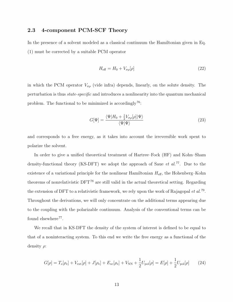
2.3 4-component PCM-SCF Theory

In the presence of a solvent modeled as a classical continuum the Hamiltonian given in Eq.

(1) must be corrected by a suitable PCM operator

Heff = H0 + Vσρ[ρ] (22)

in which the PCM operator Vσρ (vide infra) depends, linearly, on the solute density. The

perturbation is thus state-specific and introduces a nonlinearity into the quantum mechanical

problem. The functional to be minimized is accordingly76:

G[Ψ] =〈Ψ|H0 + 1

2Vσρ[ρ]|Ψ〉

〈Ψ|Ψ〉(23)

and corresponds to a free energy, as it takes into account the irreversible work spent to

polarize the solvent.

In order to give a unified theoretical treatment of Hartree–Fock (HF) and Kohn–Sham

density-functional theory (KS-DFT) we adopt the approach of Saue et al.77. Due to the

existence of a variational principle for the nonlinear Hamiltonian Heff , the Hohenberg–Kohn

theorems of nonrelativistic DFT78 are still valid in the actual theoretical setting. Regarding

the extension of DFT to a relativistic framework, we rely upon the work of Rajagopal et al.79.

Throughout the derivations, we will only concentrate on the additional terms appearing due

to the coupling with the polarizable continuum. Analysis of the conventional terms can be

found elsewhere77.

We recall that in KS-DFT the density of the system of interest is defined to be equal to

that of a noninteracting system. To this end we write the free energy as a functional of the

density ρ:

G[ρ] = Ts[ρe] + Vext[ρ] + J [ρe] + Exc[ρe] + VNN +1

2Upol[ρ] = E[ρ] +

1

2Upol[ρ] (24)

13

where the final term is the polarization energy expressed as the expectation value of the

Vσρ[ρ] operator:

Upol[ρ] = 〈0|Vσρ[ρ]|0〉 = UNe[ρ] + UeN[ρ] + Uee[ρ] + UNN (25)

In both HF and KS-DFT methods, the electron density and other quantities are obtained

from a single Slater determinant built in the one-electron basis of the molecular orbitals

(MOs) φrr=1,M . The usual notation for orbital indices will be here adopted: i, j, k . . .

for occupied MOs, a, b, c . . . for virtual MOs and p, q, r . . . for general MOs. In Second

Quantization a Slater determinant is represented by an Occupation Number Vector (ONV)80

and we will write this vector as |0〉. We choose a unitary, exponential parametrization for

|0〉:

|0〉 = exp(−κ) |0〉 (26)

where κ is an anti-Hermitian operator:

κ =∑pq

κpqp†q κ† = −κ; (27)

the orbital rotation coefficients thus constitute an anti-Hermitian matrix, κ† = −κ. The

electron density can now be written as:

ρe(r,κ) =∑pq

Dpq(κ)Ωpq(r) =∑pq

〈0| exp(κ)p†q exp(−κ)|0〉(φ†p(r)φq(r)

), (28)

The advantage of this parametrization is that the orbital rotation operator exp(−κ) en-

sures orthonormality of the one-particle orbitals without the need to introduce Lagrange

multipliers: unconstrained optimization approaches can be used and redundancies are eas-

ily identified. For closed-shell systems the orbital rotation operator may accordingly be

14

restricted to

κ =∑ai

(κaia

†i− κ∗aii†a)

(29)

The gradient of the free energy with respect to the variational parameters is

G[1]ai =

∂G

∂κ∗ai

∣∣∣∣κ=0

= −fai (30)

where we have introduced the Fock (Kohn–Sham) matrix:

fpq = fvacpq + jpq + xpq(0); fvac

pq = hpq +∑j

(gpqjj − γgpjjq) + vxc;pq (31)

The xc potential vxc;pq depends on the actual form of the exchange-correlation functional

selected (detailed expressions for LDA and GGA functionals may be found in ref.77) and γ

specifies the portion of orbital exchange to be included.

Taking a variation of the form ρ = ρe +ρN + δρe = ρe +ρN, the polarization contributions

to the Fock matrix can be derived as:

1

2

∂Upol[ρ]

∂κ∗ai

∣∣∣∣κ=0

=1

2

∫dr

δUpol

δρe(r)

∂ρe(r)

∂κ∗ai

∣∣∣∣κ=0

= −∫R3

dr

∫R3

dr′Ωai(r)M(r, r′)ρ(r′)

= −∫∂C

ds

∫∂C

ds′veai(s)κ(s, s′)φ(s′) = −

∫∂C

dsveai(s)σ(s) = −q · ve

ai

(32)

where the discretization of the cavity surface was introduced in the last step. The vepq,I

integrals appearing above are given as:

vepq,I =

∫dr−Ωpq(r)

|r − sI |(33)

Separation of the ASC into electronic and nuclear contributions leads to the matrix elements

15

jpq and xpq(0) :

jpq = qN · vepq = vN†Kve

pq (34a)

xpq(0) =

(∑tu

Dtuqetu

)· ve

pq =

(∑tu

D∗utve∗ut

)Kve

pq (34b)

The matrix elements vepq,I in Eq. (33) shall be called the uncontracted potentials, and

these are three-index quantities. A boldface notation with two indices as in vepq has to be

interpreted as an array of dimension Nts whose I-th element is the electrostatic potential

integral evaluated at the I-th cavity point. A scalar product of the type qpq · vtu is to be

interpreted accordingly, i. e. as the contraction over the cavity index:∑Nts

I qpq,Ivtu,I . The

stationarity condition for the electronic free energy is then simply:

fai = 0 ∀ (ai) (35)

meaning that the Fock matrix is block diagonal in the basis of the optimal solvated molecular

4-spinors and is thus equivalent to the spectral problem:

Fϕ = ϕε (36)

The derivation above applies equally well to relativistic and nonrelativistic Hamiltonians.

To gain further insight into the additional PCM contribution to the Fock (KS) matrix

we may expand it in a basis of 2-spinors:

ϕr =

ϕLr

ϕSr

=

NLarge∑λ=1

χLλ

0

CLλr +

NSmall∑λ=1

0

χSλ

CSλr. (37)

16

The form of the vacuum-like contribution to the Fock matrix is:

F vac =

F vac,LL F vac,LS

F vac,SL F vac,SS

(38)

where the explicit expression of each term may be found elsewhere64.

The electrostatic potential and the corresponding polarization charge at point I on the

cavity is:

vI = vNI + ve

I =Natoms∑A=1

ZA|RA − sI |

+∑pq

Dpqvepq,I (39a)

qI = qNI + qe

I =Nts∑J=1

KIJ

(Natoms∑A=1

ZA|RA − sJ |

+∑pq

Dpqvepq,J

)(39b)

and we can expand veI in our 2-spinor basis as:

veI =

∑pq

Dpqvepq,I =

∑pq

∑XY

∑κλ

CX∗κpDpqC

Yλqv

e,XYκλ,I (40)

we now define the density matrices in a 2-spinor basis as:

DXYµν =

∑pq

CX∗νp DpqC

Yµq =

∑i

CYµiC

X∗νi (41)

the last equality being valid only for a closed-shell SCF wave function. We note that the

ve,XYκλ,I are calculated over a purely multiplicative Coulomb interaction kernel that is an even

operator and hence do not couple the large and small components of 4-spinors:

ve,XYκλ,I =

∫drχX†κ (r)

−1

|r − sI |χYλ (r) = δXY

∫dr−ΩXY

κλ (r)

|r − sI |(42)

Eq. (39a) for the potential and consequently Eq. (39b) are simplified, as their matrix

17

representation is block diagonal in a 2-spinor basis:

vI = vNI + ve,LL

I + ve,SSI (43a)

qI = qNI + qe,LL

I + qe,SSI (43b)

Inserting the result in Eq. (42) in Eqs. (34a) and (34b) the 2-spinor expansion of the J

and X(0) solvent operators is obtained:

jXXκλ = qN · ve,XXκλ xXXκλ (0) = qe · ve,XX

κλ (44)

To conclude, the final form of the Fock matrix in solution is:

F =

F vac,LL + q · ve,LL F vac,LS

F vac,SL F vac,SS + q · ve,SS

(45)

where the PCM contribution appears only on its diagonal blocks.

Let us now consider possible approximations of the polarization contribution in order to

achieve computational speedups. It is well known that the most intensive task in an electronic

structure calculation is the construction of matrix elements involving two-electron integrals.

This computational bottleneck is even worse for calculations based on the Dirac-Coulomb

Hamiltonian since the number of atomic basis functions is always greater than the one in a

nonrelativistic calculation on the same system due to the small components of the molecular

4-spinor. However, due to the locality of the small component density, the calculation of

two-electron integrals of the gSSSS class can be completely avoided81. Neglecting the very

expensive gSSSS class of two-electron integrals and applying an a posteriori simple Coulombic

correction (SCC) to the energy with pretabulated or computed small component charges

leads to a negligible error in energies, structures and molecular observables.

We propose a similar approximation, called PCM-SCC, to avoid the calculation of the

18

vSS class of integrals. The electronic molecular electrostatic potential at cavity point I is:

veI =

∑κλ

DLLκλv

e,LLλκ,I +

∑κλ

DSSκλv

e,SSλκ,I '

∑κλ

DLLκλv

e,LLλκ,I +

Nnuclei∑A

qSCCA

|RA − sI |(46)

where qSCCA is the pretabulated small charge for nucleus A. Finally, in the spirit of the SCC

as proposed by Visscher81, the PCM interaction part in the SS block of the Fock matrix can

be completely neglected:

F =

F vac,LL + q · ve,LL F vac,LS

F vac,SL F vac,SS + q · ve,SS

'F vac,LL + q · ve,LL F vac,LS

F vac,SL F vac,SS

(47)

The reader may wonder why one has to bother with such approximate schemes when the

molecular electrostatic potential matrix elements are one-electron integrals, usually quite

cheap to compute. One must however bear in mind that such integrals are to be calculated

over the grid points provided by the discretization of the cavity. This implies that the

formal scaling of the PCM contributions is on the order of NtsN2 compared to N4 for the

construction of the two-electron Fock matrix. The number of tesserae Nts depends on the

molecular topology and the user-specified average tesserae area aI and is independent of the

number N of basis functions. If reduced scaling algorithms are applied to the two-electron

part such algorithms must also be applied to the PCM contribution to avoid that the latter

becomes a computational bottleneck.

2.4 Linear response for a relativistic PCM-SCF state

In order to derive the linear response function for static perturbations, we augment the free

energy functional in Eq. (23) with a perturbation operator V :

G[0] = 〈0|H0 +1

2Vσρ[ρ] + V |0〉 . (48)

19

The perturbation operator is taken to have the following form:

V =∑X

εXHX (49)

i.e. a linear combination of one-electron perturbation operators HX weighted by the pertur-

bation strengths εX . Molecular properties are then obtained as derivatives, at zero pertur-

bation strength, of the free energy with respect to the perturbation strength. We will closely

follow Sa lek et al.82, but focus on solvent contributions.

Notice that the free energy functional in Eq. (48) does not take into account nonequi-

librium effects83. It is thus not suitable for the derivation of frequency-dependent response

functions, needed for the calculation of dynamic properties and excitation energies84. We

shall address the extension of the current derivation to the nonequilibrium regime in a later

contribution.

Using the variational condition (35), second-order properties can be expressed as

d2G

dεA dεB

∣∣∣∣ε=0

=∑pq

∂2G

∂εA∂κpq

dκpqdεB

∣∣∣∣ε=0

. (50)

The first-order amplitudes are obtained from the first-order response equation

d

dεB

(∂G

∂κpq

)∣∣∣∣ε=0

=

[∂2G

∂εB∂κpq+∑rs

∂2G

∂κpq∂κrs

dκrsdεB

]ε=0

= 0 (51)

which can be recast in matrix form as

G[2]XB = −E[1]B (52)

The electronic free energy Hessian appearing in this equation has the following structure82:

G[2] =

A B

B∗ A∗

(53)

20

with the A and B matrix elements being:

∂2G

∂κ∗ai∂κbj

∣∣∣∣κ=0

= Aai,bj = δijfab − δabfji + Lγai,jb + wxc;ai,jb + qeai · ve

jb (54a)

∂2G

∂κ∗ai∂κ∗bj

∣∣∣∣∣κ=0

= Bai,bj = Lγai,bj + wxc;ai,bj + qeai · ve

bj (54b)

where

fpq = fvacpq + q · ve

pq Lγai,jb = gaijb − γgabji. (55)

The vector of apparent surface charges is given as q = qN + qe. The solvent contributions

to the A matrix are found as

Apolai,bj =

1

2

∫dr

δUpol

δρe(r)

∂2ρe(r)

∂κ∗ai∂κbj

∣∣∣∣κ=0

+

∫R3

dr

∫R3

dr′δ2Upol

δρe(r)δρe(r′)

∂ρe(r)

∂κ∗ai

∂ρe(r′)

∂κbj

∣∣∣∣κ=0

=1

2

∫dr

δUpol

δρe(r)[δijΩab(r)− δabΩji(r)]

∣∣∣∣κ=0

+

∫R3

dr

∫R3

dr′δ2Upol

δρe(r)δρe(r′)Ωai(r)Ωjb(r

′)

∣∣∣∣κ=0

= δij(q · veab)− δab(q · ve

ji) + qeai · ve

jb

(56)

and analogously for the B matrix.

The solution of the linear system in Eq. (52) is achieved by means of subspace iteration

methods85. The solution vector is expanded in a set of n trial vectors, bi, leading to the

reduced response equation, i. e. their projection in the chosen subspace. Such a method

requires repeated evaluation of the so-called σ-vector, i. e. the linear transformation of the

selected subspace by the electronic free energy Hessian.

The σ-vector formation can be reformulated as the evaluation of a generalized Fock

matrix86:

σai = −[fai + Lγai + qe · ve

ai

](57)

In these expressions a tilde indicates that a one-index transformation of the integrals by

21

means of the trial vector has to be performed. The expression of the transformed two-

electron term Lγrs is given elsewhere86,87. What is to be noted here is that it can be evaluated

by contraction of the usual two electron integrals with a perturbed AO basis one-electron

density, obtained by transformation with the trial vectors. A similar approach can be used

in evaluating the one-index transformed polarization charges:

qe = K

[∑κλ

Dκλveλκ

]Dκλ = −

∑ut

CuλbutC∗tκ (58)

3 Implementation

The solution of the electrostatic problem posed by the addition of a polarizable continuum

surrounding the molecular solute, requires a limited number of steps which are independent

of the nature of the electronic-structure method employed. These steps, namely, cavity for-

mation and discretization together with formation of the PCM matrix K, can be abstracted

from the structure of the program performing the optimization of the electronic structure.

This modular programming paradigm is not new88,89, but is a very powerful strategy to

effectively enable code reuse throughout altogether different quantum chemical programs.

In Figure 1 we show the PCM-SCF algorithm one needs to implement. The neat sepa-

ration between PCM-related and QM-related tasks is shown, the only additional step added

with respect to a conventional in vacuo SCF algorithm being the evaluation of the molecular

electrostatic potential at the grid points provided by the discretized molecular cavity.

The existence of this separation between the classical electrostatic problem and the quan-

tum problem for the optimization of the electronic structure, led us to the implementation

of a standalone module for the PCM, which we have called PCMSolver61. PCMSolver is

intended to be an application programming interface (API) providing all the functionality

needed to handle the PCM electrostatic problem: generation and discretization of the cav-

ity, generation of the PCM matrix. Both tasks can be performed in a fully general manner:

22

Molecular electrostaticpotential at the cavity:vI =

∑A

ZA|RA−sI |

+∑κλDλκ

[∫dr−Ωκλ(r)

|r−sI |

]

Apparent Surface Charge:q = Kv

Polarization energy:Upol = q · v

Fock matrix:fκλ = fvac

κλ + q · veκλ

SCFconverged?

Finalize SCF

yes

no

Cavity

Geometry, D

BE solver

Figure 1: Schematic view of the implemented SCF algorithm. Computations/data in blueare on the PCMSolver side, in green on the DIRAC side.

isotropic and anisotropic environments can be treated, and are accommodated within the

same general code infrastructure, thus reflecting the derivation of the IEF-PCM equation

given by Cances et al.72 in their seminal paper. Treatment of diffuse interfaces is also pos-

sible90. The newly implemented Boundary Element solver based on a wavelet formalism is

made available within the same framework91–93.

The concept of data hiding is effectively enforced: only the necessary functions are visible

to the end-user of our API through an interface. The major coding effort in interfacing

PCMSolver to any quantum chemical program regards the efficient evaluation of the molecular

electrostatic potential. We would like to stress the point that through the use of our API,

virtually any quantum chemical program package could introduce a continuum description

23

of the solvent. Our approach has two main advantages over an in-house coding of the PCM:

1. coding effort is minimized, because the necessary functions already come bundled in a

compact library. Furthermore, these functions are already tested, only the QM-PCM

interface is to be tested;

2. new PCM functionalities, such as novel algorithms for the cavity generation and the

solution of the electrostatic problem, as well as additional environments, can be added

to the API without touching the QM code. These new functionalities will be seamlessly

and immediately available to the QM program, with a negligible amount of work.

3.1 4-component Molecular Electrostatic Potential

As shown in Section 2.1, the addition of relativity is irrelevant for the generic algorithm

which is suitable for both nonrelativistic and relativistic calculations. The only difference in

the latter case is in the calculation of the contracted electrostatic potential

veI =

∑pq

Dpqvepq,I , (59)

In a scalar atomic basis, we need to calculate the integrals

vIκλ(sI) =

∫dr−Ωκλ(r)

|r − sI |. (60)

where sI is a point on the cavity surface. Such integrals are identical to the ordinary nuclear-

attraction integrals, but have a different physical origin and should rather be called charge-

attraction integrals. We recall that only the LL and SS sub-blocks need to be evaluated.

The implementation of Eq. (60) requires looping over basis functions and grid points.

The loop over grid points may be placed either outside or inside the two basis function

loops. The former choice is easier to implement but generates a highly inefficient code, due

to the large number of intermediate quantities that needs to be recalculated for each grid

24

point. The latter is instead more efficient because it can be seen as a form of vectorization,

where each iteration over the basis function, an entire batch of points (the whole grid in

our case), is computed instead of one point at a time. Intermediates are in this case reused

and a full exploitation of compiler optimization is possible. The vectorization will also

enable a relatively straightforward port of the code to architectures based on General-purpose

computing on graphics processing units (GPGPU).

This second approach is the one used in our implementation in the DIRAC code60. As

a useful by-product, molecular electrostatic potential maps are available for 4-component

electronic-structure calculations. To the best of our knowledge, this is the first implementa-

tion of such a visualization and analysis tool in a relativistic 4-component framework.

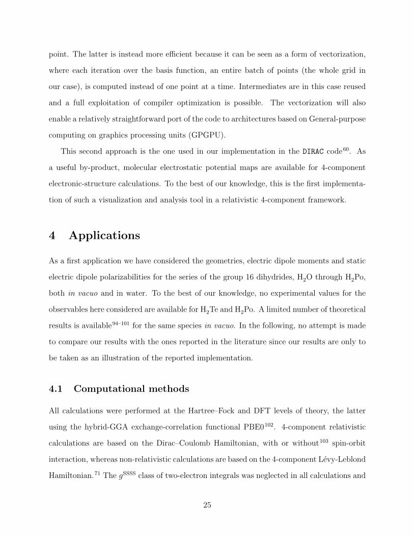
4 Applications

As a first application we have considered the geometries, electric dipole moments and static

electric dipole polarizabilities for the series of the group 16 dihydrides, H2O through H2Po,

both in vacuo and in water. To the best of our knowledge, no experimental values for the

observables here considered are available for H2Te and H2Po. A limited number of theoretical

results is available94–101 for the same species in vacuo. In the following, no attempt is made

to compare our results with the ones reported in the literature since our results are only to

be taken as an illustration of the reported implementation.

4.1 Computational methods

All calculations were performed at the Hartree–Fock and DFT levels of theory, the latter

using the hybrid-GGA exchange-correlation functional PBE0102. 4-component relativistic

calculations are based on the Dirac–Coulomb Hamiltonian, with or without103 spin-orbit

interaction, whereas non-relativistic calculations are based on the 4-component Levy-Leblond

Hamiltonian.71 The gSSSS class of two-electron integrals was neglected in all calculations and

25

r r

z ≡ C2

x

θ

Figure 2: Geometric parameters and orientation of the H2X species considered. The positivey axis points outside the xz-plane.

Visscher’s simple Coulombic correction81 adopted throughout.

A development version of the 4-component relativistic molecular code DIRAC, interfaced

with the PCMSolver module, was used. Uncontracted, triple-zeta quality basis sets were

used for the large components: cc-pVTZ for H, O, S104,105 and dyall.v3z106–108 for Se, Te,

Po. Restricted kinetic balance was applied to obtain the small component basis set.

In all calculations, the dihydrides are placed in the xz-plane, the C2 rotation axis is along

the z axis, with the direction of the positive z axis from the heavy atom to the hydrogens,

as shown in Figure 2.

The structures were optimized using the numerical molecular gradient evaluated by means

of finite differences. The general driver for structure optimizations in DIRAC is the same as in

the nonrelativistic code DALTON109,110. The structures optimized in vacuo using the numerical

gradient were compared with those obtained using the analytic gradient. Bond lengths, bond

angles and energies obtained with the two methods were found to be in good agreement: for

Hartree–Fock calculations, the average relative error in bond lengths and bond angles is 80

ppm, while that on energies is 50 ppb. Based on these results, we have assumed the numerical

gradient optimizations to be reliable also for solvent calculations, where an analytic gradient

is not yet available.

Water, with relative dielectric constant εr = 78.39, was selected as solvent. The cavities

were generated using the Bondi–Mantina set of van der Waals radii111. The radii used 1.20

A for H, 1.52 A for O, 1.80 A for S, 1.90 A for Se, 2.06 A for Te and 1.97 A for Po. These

26

radii were then multiplied by a scaling factor of 1.2 as usual in the application of the PCM112.

The cavities were obtained without the addition of spheres not centered on the nuclei. A fine

tessellation, with average tessera area of 0.3a20 ' 0.084A2, was chosen. For H2O and H2Po,

we investigated the effect of tessellation (not shown) and found our results converged for this

value of the average tessera area, as could have been expected from non-relativistic studies.

For further discussion of tessellation and other technical issues related to the implementation

of the polarizable continuum model, we refer to10,11,112. For general comments on boundary

element methods for integral equations, such as discretization techniques and convergence

estimates, we refer to the book by Hackbusch74.

For electronic structure analysis we have employed projection analysis100 using the pre-

calculated in vacuo orbitals of the constituent atoms.

4.2 Assessment of the PCM-SCC approximation

The possibility to skip the evaluation of the SS block of the electrostatic potential integrals

as described in Section 2.3, was implemented (.SKIPSS input keyword). By default, these

integrals are not skipped. To assess the impact of the PCM-SCC approximation, geometry

optimizations were performed for H2Po, both at the Hartree–Fock and DFT/PBE0 levels

of theory. Subsequent single-point calculations employing the “full” Dirac–Coulomb model

and the approximate PCM-SCC model were performed, taking the geometry optimized with

the “full” model as reference.

Tables 1 and 2 summarize the results obtained for geometries, energies and CPU times.

All calculations were performed on a single node equipped with two Xeon E5-2670@2.60

GHz octacore processors. The MPI-parallel version of the code was used. The geometries

predicted with the proposed approximation to the electrostatic potential integrals fully agree

with the ones obtained with the “full” model. The agreement between calculated energies

is also found to be acceptable. Although the formation of the PCM contribution to the

Fock matrix was not found to be the most time consuming step in our test case, the timings

27

reported in Table 2 suggests that it may be beneficial to employ the PCM-SCC approximation

in those cases where one or both of the following conditions apply: a) a large number of small

component basis functions is used; b) a large number of finite elements is used to discretize

the PCM cavity. All the calculations presented in the rest of this work were performed

without resorting to the PCM-SCC approximation.

Table 1: Differences in bond distance, bond angle and free energy between theDirac–Coulomb and Dirac–Coulomb PCM-SCC results for H2Po. Single-pointcalculations performed on the geometry optimized with the Dirac–CoulombHamiltonian.

∆r / A ∆θ / ∆G / Eh

Hartree–Fock -0.00001 0.002 0.000003DFT/PBE0 -0.00002 -0.001 0.000007

Table 2: Average CPU time elapsed in an SCF iteration, tSCF, and in the forma-tion of the PCM contribution to the Fock matrix, tPCM. The number of iterationsneeded to reach convergence, Nit is also reported. All timings in seconds, calcu-lations performed on a single node equipped with two Xeon E5-2670@2.60 GHzoctacore processors. The system studied was H2Po.

Dirac–Coulomb Dirac–Coulomb PCM-SCC

tSCF tPCM Nit tSCF tPCM Nit

Hartree–Fock 43.16 4.90 27 35.47 0.86 21DFT/PBE0 47.62 5.40 19 38.22 0.90 18

As illustrated in Figure 1, in each SCF cycle we perform the following steps:

1. we form the uncontracted potentials Eq. (33) and immediately contract them with the

density matrix, to obtain the potential at cavity points. Here we have a saving since

the SS block is neglected and approximated with a SCC-like correction;

2. the polarization charges are calculated. This is a call to PCMSolver that performs a

matrix-vector multiplication. There is no saving here as this depends solely on the

dimension of the cavity which is unaffected by skipping the SS block;

28

3. we again form the uncontracted potentials Eq. (33) and immediately contract them

with the polarization charges, to obtain the PCM contribution to the Fock matrix.

Here we have a saving since there is no SS block, see Eq. (47);

The reader may notice that in each SCF cycle, there is an additional time saving, not

accounted for by the savings in tPCM. This is because in each SCF step the PCM-SCC

approximation has an impact both in the initial formation of the potential at cavity points

and in the formation of the PCM contribution to the Fock matrix.

4.3 Relativistic effects associated with the PCM model

Key parameters in the PCM model are the atomic radii used for the generation of the molecu-

lar cavity. As already stated we have in the present work employed the Bondi–Mantina set of

van der Waals radii111 scaled by a factor of 1.2, consistent with previous PCM calculations.112

Whereas Bondi extracted his recommended van der Waals radii from contact distances from

X-ray diffraction studies of (mostly) molecular crystals,113 Mantina et al. extended the tables

by calculations of the repulsive wall distance with respect to neutral, closed-shell probes.111

The radii for the heavier elements were obtained using the Douglas-Kroll-Hess Hamiltonian

including scalar relativistic effects only. It would be worth investigating the trend in van

der Waals radii when considering more complete Hamiltonian models, in particular for the

heavier p-block elements where second-order spin-orbit effects, affecting orbital sizes, are

substantial, but this is outside the scope of the present contribution.

It should also be noted that the apparent surface charges in the PCM model will induce a

spin-orbit effect in addition to those generated by the relative motion of a reference electron

and other charges, electrons and nuclei, in the system.63 This effect is difficult to quantify,

but we observe that for H2Po, at the optimized DC/PBE0 geometry in water, the magnitude

of the solvation energy is reduced by ' 15% when the spin-orbit interaction is turned off,

albeit most of this effect probably arises from the modification of the electron density.

29

4.4 Geometries and electric dipole moments

Table 3 presents the results regarding the geometries and electric dipole moments obtained

at the Hartree–Fock and DFT/PBE0 levels of theory. Only the z-component of the electric

dipole moment is reported, since the x- and y-components are zero by symmetry.

We recall that the I-th component of the electric dipole moment is defined as the first

derivative of the (free) energy with respect to the I-th component of an applied electric field

F 114, which is equivalent, in the case of SCF methods, to the calculation of the expectation

value of the electric dipole operator:

µI = − ∂E(F )

∂FI

∣∣∣∣F=0

= 〈0 | µI | 0〉 (61)

Table 3: Bond lengths, bond angles and z-components of the electric dipolemoment.

Dirac–Coulomb Spin-free Levy-Leblond

r / A θ / µz / D r / A θ / µz / D r / A θ / µz / D

Hartree–Fock

In vacuo

H2O 0.940 105.9 1.985 0.940 105.9 1.985 0.941 106.0 1.988H2S 1.329 94.1 1.142 1.329 94.1 1.143 1.330 94.2 1.160H2Se 1.451 92.9 0.779 1.451 92.9 0.782 1.454 93.2 0.858H2Te 1.649 92.1 0.293 1.648 92.2 0.312 1.656 92.7 0.495H2Po 1.742 90.8 -0.575 1.725 91.2 -0.311 1.754 92.6 0.261

Water

H2O 0.944 104.9 2.296 0.944 104.9 2.296 0.944 104.9 2.299H2S 1.331 94.9 1.484 1.331 94.9 1.484 1.331 95.0 1.505H2Se 1.452 93.7 1.082 1.452 93.7 1.085 1.455 94.0 1.182H2Te 1.649 92.6 0.485 1.648 92.6 0.508 1.657 93.4 0.758H2Po 1.746 90.0 -0.832 1.728 90.7 -0.444 1.754 92.7 0.398

DFT/PBE0

In vacuo

H2O 0.958 104.3 1.923 0.958 104.3 1.923 0.958 104.4 1.926H2S 1.344 92.2 1.118 1.344 92.2 1.118 1.344 92.3 1.136H2Se 1.465 90.8 0.719 1.465 90.8 0.722 1.467 91.1 0.801H2Te 1.661 90.2 0.239 1.660 90.2 0.259 1.667 90.8 0.447H2Po 1.759 89.3 -0.577 1.738 89.7 -0.324 1.762 90.8 0.233

Water

H2O 0.962 103.3 2.249 0.962 103.3 2.249 0.962 103.4 2.252H2S 1.346 93.1 1.466 1.346 93.1 1.466 1.346 93.2 1.488H2Se 1.467 91.6 1.009 1.466 91.6 1.012 1.469 92.0 1.114H2Te 1.662 90.7 0.409 1.661 90.7 0.433 1.668 91.5 0.694H2Po 1.764 88.9 -0.842 1.741 89.1 -0.477 1.763 91.0 0.351

Trends in bond lengths and bond angles along the periods are reported in Figure 3 and

30

Figure 4, respectively. The geometries predicted at the Hartree–Fock level of theory show

shorter bond lengths and larger bond angles than the ones predicted using DFT/PBE0. A

monotonic increase in bond length, correlating with the size of the central atom, is observed

going down in the group. No deviations from this trend are observed, neither including

relativity, nor considering the solvent. Scalar relativistic effects tend, as expected, to shorten

bonds. Spin-orbit effects only become dramatic for H2Po: At the DFT/PBE0/in vacuo level

of theory scalar relativity shortens the bond by 0.024 A, whereas spin-orbit interaction

increases the bond length by 0.021 A, almost back to the non-relativistic value.

Figure 4 clearly shows a marked reduction in bond angle beyond water, which constitutes

a well-known failure of the valence shell electron pair repulsion (VSEPR) model. These

observations agree with the study by Dubillard et al.100, where a detailed discussion is

provided. The effect of the solvent on molecular geometries is seen to be rather small: bond

lengths increase slightly, whereas there is no clear trend for bond angles.

0.9

1

1.1

1.2

1.3

1.4

1.5

1.6

1.7

1.8

2 3 4 5 6

r/

A

Period

In vacuo WaterDirac–Coulomb

Spinfree

Levy-Leblond

Figure 3: Optimized bond lengths at the DFT/PBE0 level of theory. Dot-dashed lines: invacuo calculations. Solid lines: water calculations.

Figure 5 shows a uniform trend of decreasing dipole moment with the period, which

clearly correlates with the reduction of the electronegativity of the central atom when going

down the group94. From projection analysis100 we accordingly find at the DC/PBE0/vacuum

31

85

90

95

100

105

2 3 4 5 6

θ/

Period

In vacuo WaterDirac–Coulomb

Spinfree

Levy-Leblond

Figure 4: Optimized bond angles at the DFT/PBE0 level of theory. Dot-dashed lines: invacuo calculations. Solid lines: water calculations.

level a charge of−0.98e on oxygen in H2O (µz = +1.923D), whereas the corresponding charge

on polonium in H2Po (µz = −0.577D) is +0.07e. The situation is somewhat more complex,

though, because at the non-relativistic level the corresponding charge on polonium is almost

the same (+0.11e), but now the dipole moment is positive (µz = +0.233D). This means

that the inclusion of relativity switches the sign of the dipole moment in H2Po, although

the molecular geometry and atomic charges hardly change. In order to better understand

this seeming paradox, we first recall that the electronic and nuclear contributions separately

depend on the origin. Placing the origin of the dipole moment on the central atom, the

nuclear contribution from polonium is identically zero, and the electronic contribution is

essentially limited to four valence orbitals, associated with the two bonds and two lone

pairs. After Pipek-Mezey localization we find that the weight of polonium in the bonding

orbitals is 46.6%, 47.6% and 45.8% at the Dirac-Coulomb, spin-free and non-relativistic

levels, respectively, showing that the polarity of the bonds is essentially independent of the

choice of Hamiltonian, thus further adding to the enigma. However, the matrix elements of

the 6s and 6pz orbitals over the µz-operator are significantly reduced with the introduction

of scalar relativity, due to orbital contraction. This affects the lone pair orbitals more than

32

the bonding ones: their contribution to the z-component of the dipole moment is thereby

reduced from 4.78D to 3.40D, whereas the contribution from the two bonding orbitals to

the z-component of the dipole moment changes from −16.26D to −15.26D. This explains

the change of sign of the dipole moment. With the introduction of spin-orbit coupling the

6p3/2 and 6p1/2 components expand and contract, respectively, with respect to the spinfree

6p orbital, but the sign of the dipole moment is conserved.

The inclusion of solvent significantly increases the magnitude of dipole moments for all

species and with respect to all Hamiltonians included, a trend already present in Onsager’s

model115. Since the molecular geometries of the studied molecules are only slightly affected,

this is clearly an electronic effect. For H2Po at the DC/PBE0 level the dipole moment changes

from −0.577D to −0.842D, indicating an electronic charge transfer to the hydrogens. From

projection analysis we indeed find that the polonium charge increases slightly (+0.07e →

+0.08e), whereas the polarity of the bonds hardly changes.

-1

-0.5

0

0.5

1

1.5

2

2 3 4 5 6

µz

/D

Period

In vacuo WaterDirac–Coulomb

Spinfree

Levy-Leblond

Figure 5: z-component of the electric dipole moment at the DFT/PBE0 level of theory.Dot-dashed lines: in vacuo calculations. Solid lines: water calculations.

Since bond lengths are affected neither by relativity nor by solvation, the solvent effect on

these species is neatly summarized by saying that the existing charge separation is enhanced.

This is strikingly demonstrated by the electrostatic potential maps in Figure 6 where the

33

hydrogens of H2O (H2Po) are seen to become more positive (negative), although it should

be kept in mind that the electrostatic potential in a point is a weighted average of the charge

density over all space.116

(a) H2O: MEPPCM−DC −MEPDC (b) H2Po: MEPPCM−DC −MEPDC

Figure 6: Molecular electrostatic potential (MEP) maps for H2O and H2Po at theDFT/PBE0 level of theory. The isocontours are in the range [−0.02, 0.02]Ehe

−1 and arecolor-coded from red to blue. The values plotted are differences between the values obtainedfor the Hamiltonians referred to in the subcaptions. The geometry optimized in vacuo, us-ing the Dirac-Coulomb Hamiltonian as reference. PCM-DC: Dirac-Coulomb in water, DC:Dirac-Coulomb in vacuo.

4.5 Electric dipole moment polarizabilities

The components of the static electric dipole polarizability tensor are defined in terms of the

linear response function as114, i.e. as the second derivative of the (free) energy with respect

to an applied electric field F :

αIJ = −〈〈µI ;µJ〉〉 = − ∂2E(F )

∂FI∂FJ

∣∣∣∣F=0

(62)

34

where µI is the I-th component of the electric dipole operator. The isotropic part is

αiso =1

3(αxx + αyy + αzz) (63)

whereas the anisotropic part is defined as

αaniso =1√2

[(αxx − αyy)2 + (αxx − αzz)2 + (αyy − αzz)2 + 6

(α2xy + α2

xz + α2yz

)]1/2(64)

In the present case the off-diagonal components of the polarizability tensor are zero by

symmetry. Table 4 summarizes results obtained for the diagonal components as well as

αiso and αaniso. In Figure 7 αiso is shown as a function of the period, at the DFT/PBE0

level of theory. A striking feature is the almost complete lack of relativistic effects on the

electric dipole polarizability. This can, however, be understood from the connection between

αiso and molecular volume. In fact, from Figure 7 one may apprehend the more compact

molecular structure of spin-free H2Po compared to the non-relativistic and fully relativistic

counterparts. It should be noted, though, that this observation is far from general. Whenever

relativity significantly modifies the spatial extent of valence orbitals, one may also expect

large relativistic effects on the electric dipole polarizability, as reported for example for

HgS117.

For the solvated systems, αiso is always significantly greater (' 70%) than in vacuo. This

is not unexpected as in solvent a greater charge separation was observed from the trends

in dipole moments. The modification by the inclusion of solvent of individual components

of the polarizability tensor is not uniform, though, and leads to less obvious trends for the

polarizability anisotropy which are harder to rationalize, as seen from Figure 8. The signif-

icant change in the the polarizability anisotropy at the spinfree PBE0 level upon inclusion

of solvent arises from the 90% increase of the αyy (out-of-plane) component compared to a

60% increase of αxx and αzz.

35

0

2

4

6

8

10

12

2 3 4 5 6

αis

o/

A3

Period

In vacuo WaterDirac–Coulomb

Spinfree

Levy-Leblond

Figure 7: Isotropic electric dipole polarizability at the DFT/PBE0 of theory. Dot-dashedlines: in vacuo calculations. Solid lines: water calculations.

0

0.2

0.4

0.6

0.8

1

2 3 4 5 6

αan

iso

/A

3

Period

In vacuo WaterDirac–Coulomb

Spinfree

Levy-Leblond

Figure 8: Anisotropic electric dipole polarizability at the DFT/PBE0 of theory. Dot-dashedlines: in vacuo calculations. Solid lines: water calculations.

36

Table 4: Isotropic, anisotropic and Cartesian components of the electric dipole polarizability tensor. All valuesare reported in A3.

Dirac–Coulomb Spin-free Levy-Leblond

αiso αaniso αxx αyy αzz αiso αaniso αxx αyy αzz αiso αaniso αxx αyy αzz

Hartree–Fock

In vacuo

H2O 0.959 0.334 1.147 0.762 0.967 0.959 0.334 1.147 0.762 0.967 0.958 0.333 1.146 0.762 0.965H2S 2.715 0.654 3.021 2.293 2.831 2.715 0.654 3.021 2.293 2.831 2.712 0.655 3.020 2.289 2.825H2Se 3.657 0.558 3.927 3.300 3.743 3.655 0.554 3.924 3.301 3.741 3.654 0.572 3.938 3.292 3.733H2Te 5.427 0.393 5.649 5.196 5.436 5.421 0.364 5.632 5.211 5.420 5.464 0.439 5.731 5.227 5.434H2Po 6.201 0.729 6.490 5.718 6.394 6.130 0.312 6.288 5.934 6.167 6.289 0.607 6.643 5.942 6.282

Water

H2O 1.075 0.363 1.277 0.858 1.091 1.075 0.363 1.277 0.858 1.091 1.074 0.363 1.275 0.857 1.090H2S 3.443 0.832 3.850 2.913 3.567 3.443 0.832 3.850 2.913 3.567 3.437 0.833 3.847 2.907 3.557H2Se 4.871 0.667 5.225 4.461 4.925 4.868 0.661 5.220 4.463 4.922 4.864 0.691 5.240 4.445 4.906H2Te 7.696 0.449 7.992 7.508 7.587 7.688 0.412 7.962 7.537 7.565 7.755 0.559 8.128 7.562 7.575H2Po 9.452 1.010 9.858 8.784 9.715 9.346 0.169 9.455 9.312 9.270 9.631 0.790 10.152 9.305 9.436

DFT/PBE0

In vacuo

H2O 1.046 0.362 1.241 0.826 1.071 1.046 0.362 1.241 0.826 1.071 1.045 0.362 1.240 0.825 1.069H2S 2.796 0.667 3.072 2.356 2.961 2.796 0.667 3.071 2.356 2.961 2.792 0.668 3.069 2.351 2.955H2Se 3.770 0.504 3.975 3.437 3.898 3.769 0.499 3.972 3.439 3.895 3.764 0.524 3.984 3.419 3.890H2Te 5.573 0.263 5.693 5.403 5.624 5.567 0.228 5.674 5.420 5.607 5.593 0.320 5.760 5.395 5.625H2Po 6.372 0.546 6.550 6.008 6.557 6.310 0.100 6.350 6.243 6.336 6.423 0.466 6.656 6.128 6.485

Water

H2O 1.180 0.399 1.390 0.933 1.216 1.180 0.399 1.390 0.933 1.216 1.178 0.399 1.388 0.932 1.214H2S 3.567 0.846 3.930 3.012 3.760 3.567 0.846 3.930 3.012 3.760 3.560 0.847 3.926 3.005 3.750H2Se 5.069 0.553 5.317 4.709 5.182 5.067 0.546 5.312 4.712 5.178 5.056 0.587 5.327 4.676 5.164H2Te 7.995 0.147 8.092 7.954 7.939 7.986 0.127 8.059 7.989 7.912 8.023 0.273 8.204 7.930 7.933H2Po 9.843 0.526 10.014 9.492 10.023 9.766 0.490 9.592 10.092 9.614 9.969 0.385 10.220 9.797 9.891

37

4.6 Choice of solvent

In the above calculations water, with relative dielectric constant εr = 78.39, was selected

as solvent. It may be objected that specific interactions of a protic solvent such as water

and the solute will be important and are not captured by a continuum model such as PCM.

However, this will depend to what extent specific interactions such as hydrogen bonding are

important for the property under study. Continuum models such as PCM have been widely

applied to describe aqueous solution, in most cases with quite satisfactory results26,50. To

rigorously demonstrate shortcomings of our relativistic results, due to the persistence and

importance of specific interactions over time, would require molecular dynamics simulations

with a statistically significant sampling21,118, a computational protocol which is not presently

available at the 4-component relativistic level. It should also to be noted that the present

implementation only includes contributions of electrostatic origin, neglecting dispersion, re-

pulsion119 and cavitation120 contributions: a fair comparison between continuum and explicit

models has to take into account all energy contributions.

In figure 9 we display the electric dipole moment and isotropic dipole polarizability of

H2Po, relative to vacuum values, as a function of relative permittivity εr. The vacuum

optimized molecular geometry was employed, since solvent effects on geometries were found

to be small. Given the solutes considered in this study we do not expect nonlinearities121

in the solvent effect, hence lower polarity solvents should yield a reduced effect with values

that are “bracketed” by the gas-phase and water ones. This is indeed what we observe, as

well as the well-known saturation of dielectric response122,123. The relative difference of the

observables can be perfectly fitted (correlation coefficient 1) to a linear rational function,

that is

X(εr)−X(1) =εr − 1

aεr + bX(1); X = µz, αiso (65)

For H2Po the values (a, b) of the fit coefficients are (2.339, 3.140) and (1.797, 2.345) for µz

and αiso, respectively. These values are system-dependent; with water as solute we obtain

38

1

1.1

1.2

1.3

1.4

1.5

1.6

0 10 20 30 40 50 60 70 80Relative permittivity

µzαiso

Figure 9: Electric dipole and isotropic dipole polarizability of H2Po, relative to vacuumvalues, as a function of relative permittivity εr.

(6.150, 3.942) and (8.084, 5.251).

5 Conclusions

A detailed derivation of the Polarizable Continuum Model for 4-component Hartree–Fock

and Kohn–Sham calculations has been presented. The derivation of the first-order response

equation including the contributions from a polarizable continuum has also been detailed.

The algorithm implemented has been described and in particular the advantages of the

modular programming paradigm adopted have been elucidated. This new functionality im-

plemented in the DIRAC program package will be made available in the DIRAC14 release. We

would like to stress the importance of modularity for the work here presented. Use of the

flexible API library PCMSolver has effectively enabled us to use a tested and standardized

implementation of the PCM related tasks in the more general framework of 4-component

electronic-structure theory. PCMSolver clearly implements the emerging ideas in modern

programming techniques, such as abstraction, data hiding and, above all, code reusability.

39

The few results summarized in this paper show some of the many potential applications

of the 4-component PCM-SCF scheme. Calculation of excitation energies using our LR-

PCM-SCF algorithm is possible with a small additional coding effort, in order to properly

take into account the effect of nonequilibrium solvation on the excitation process11. Fur-

ther developments of the work here presented regard the calculation of parameters relevant

for magnetic spectroscopies and the extension to 2-component Hamiltonian models63. Both

lines of development are currently being investigated.

Acknowledgement

This paper is dedicated to Prof. Jacopo Tomasi on the occasion of his 80th birthday. One of

the authors (L.F.) has had the privilege to graduate under Tomasi’s supervision, appreciating

his passion for science, his curiosity for new developments and his immense knowledge of the

scientific literature. The authors would like to thank Prof. Benedetta Mennucci for useful

discussions. R.D.R. gratefully acknowledges the financial support from the Erasmus Lifelong

Learning Programme during his stay in Toulouse. This work has been supported by the

Research Council of Norway through a Centre of Excellence Grant (Grant No. 179568/V30)

and through a NOTUR allocation of computer resources (Grant No. NN4654K).

References

(1) Dirac, P. A. M. Quantum Mechanics of Many-Electron Systems. Proc. Roy. Soc. Lond.

A 1929, 123, 714–733.

(2) Kutzelnigg, W. Perspective on ”Quantum Mechanics of Many-Electron Systems”.

Theor. Chem. Acc. 2000, 103, 182–186.

(3) Markus, R.; Wolf, A. Relativistic Quantum Chemistry ; Wiley-VCH Verlag GmbH &

Co. KGaA, 2009.

40

(4) Pyykko, P. Relativistic Effects in Chemistry: More Common Than You Thought.

Annu. Rev. Phys. Chem. 2012, 63, 45–64.

(5) Glantschnig, K.; Ambrosch-Draxl, C. Relativistic Effects on the Linear Optical Prop-

erties of Au, Pt, Pb and W. New. J. Phys. 2010, 12, 103048–103064.

(6) Reichardt, C.; Welton, T. Solvents and Solvent Effects in Organic Chemistry ; Wiley-

VCH Verlag GmbH & Co. KGaA, 2010.

(7) Hansen, J.-P.; McDonald, I. R. Theory of Simple Liquids ; Academic Press: Burlington,

2006.

(8) Hill, T. L. An Introduction to Statistical Thermodynamics ; Dover Publications, Inc.:

New York, 1986.

(9) Tomasi, J. In Continuum Solvation Models in Chemical Physics ; Mennucci, B.,

Cammi, R., Eds.; John Wiley & Sons, Ltd, 2007; pp 1–28.

(10) Mennucci, B., Cammi, R., Eds. Continuum Solvation Models in Chemical Physics ;

John Wiley & Sons, Ltd, 2007.

(11) Tomasi, J.; Mennucci, B.; Cammi, R. Quantum Mechanical Continuum Solvation

Models. Chem. Rev. 2005, 105, 2999–3094.

(12) Senn, H. M.; Thiel, W. QM/MM Methods for Biomolecular Systems. Angew. Chem.

Int. Edit. 2009, 48, 1198–1229.

(13) Curutchet, C.; Munoz Losa, A.; Monti, S.; Kongsted, J.; Scholes, G. D.; Mennucci, B.

Electronic Energy Transfer in Condensed Phase Studied by a Polarizable QM/MM

Model. J. Chem. Theory Comput. 2009, 5, 1838–1848.

(14) Olsen, J. M.; Aidas, K.; Kongsted, J. Excited States in Solution through Polarizable

Embedding. J. Chem. Theory Comput. 2010, 6, 3721–3734.

41

(15) Steindal, A. H.; Ruud, K.; Frediani, L.; Aidas, K.; Kongsted, J. Excitation Energies

in Solution: The Fully Polarizable QM/MM/PCM Method. J. Phys. Chem. B 2011,

115, 3027–3037.

(16) Lipparini, F.; Barone, V. Polarizable Force Fields and Polarizable Continuum Model:

A Fluctuating Charges/PCM Approach. 1. Theory and Implementation. J. Chem.

Theory Comput. 2011, 7, 3711–3724.

(17) Caprasecca, S.; Curutchet, C.; Mennucci, B. Toward a Unified Modeling of Envi-

ronment and Bridge-Mediated Contributions to Electronic Energy Transfer: A Fully

Polarizable QM/MM/PCM Approach. J. Chem. Theory Comput. 2012, 8, 4462–4473.

(18) Morss, L., Edelstein, N., Fuger, J., Katz, J., Eds. The Chemistry of the Actinide and

Transactinide Elements ; Springer, 2011.

(19) Vallet, V.; Macak, P.; Wahlgren, U.; Grenthe, I. Actinide Chemistry in Solution,

Quantum Chemical Methods and Models. Theor. Chem. Acc. 2006, 115, 145–160.

(20) Schreckenbach, G.; Shamov, G. A. Theoretical Actinide Molecular Science. Acc. Chem.

Res. 2010, 43, 19–29.

(21) Mennucci, B.; Martınez, J.; Tomasi, J. Solvent Effects on Nuclear Shieldings: Contin-

uum or Discrete Solvation Models to Treat Hydrogen Bond and Polarity Effects? J.

Phys. Chem. A 2001, 105, 7287–7296.

(22) Vicha, J.; Patzschke, M.; Marek, R. A Relativistic DFT Methodology for Calculat-

ing the Structures and NMR Chemical Shifts of Octahedral Platinum and Iridium

Complexes. Phys. Chem. Chem. Phys. 2013, 15, 7740–7754.

(23) Standara, S.; Malinakova, K.; Marek, R.; Marek, J.; Hocek, M.; Vaara, J.; Straka, M.

Understanding the NMR Chemical Shifts for 6-Halopurines: Role of Structure, Solvent

and Relativistic Effects. Phys. Chem. Chem. Phys. 2010, 12, 5126–5139.

42

(24) Moncho, S.; Autschbach, J. Relativistic Zeroth-Order Regular Approximation Com-

bined with Nonhybrid and Hybrid Density Functional Theory: Performance for NMR

Indirect Nuclear Spin–Spin Coupling in Heavy Metal Compounds. J. Chem. Theory

Comput. 2010, 6, 223–234.

(25) Hay, P. J.; Martin, R. L.; Schreckenbach, G. Theoretical Studies of the Properties and

Solution Chemistry of AnO2+2 and AnO+

2 Aquo Complexes for An = U, Np, and Pu.

J. Phys. Chem. A 2000, 104, 6259–6270.

(26) Vallet, V.; Wahlgren, U.; Schimmelpfennig, B.; Moll, H.; Szabo, Z.; Grenthe, I. Solvent

Effects on Uranium(VI) Fluoride and Hydroxide Complexes Studied by EXAFS and

Quantum Chemistry. Inorg. Chem. 2001, 40, 3516–3525.

(27) Siboulet, B.; Marsden, C. J.; Vitorge, P. A Theoretical Study of Uranyl Solvation:

Explicit Modelling of the Second Hydration Sphere by Quantum Mechanical Methods.

Chem. Phys. 2006, 326, 289–296.

(28) Barakat, K. A.; Cundari, T. R.; Rabaa, H.; Omary, M. A. Disproportionation of

Gold(II) Complexes: A Density Functional Study of Ligand and Solvent Effects. J.

Phys. Chem. B 2006, 110, 14645–14651.

(29) Liao, Y.; Ma, J. Stacking and Solvent Effects on the Electronic and Optical Properties

of Gold and Mercury Acetylide Aggregations: A Theoretical Study. Organometallics

2008, 27, 4636–4648.

(30) Periyasamy, G.; Remacle, F. Ligand and Solvation Effects on the Electronic Properties

of Au55 Clusters: A Density Functional Theory Study. Nano Lett. 2009, 9, 3007–3011.

(31) Vallet, V.; Grenthe, I. On the Structure and Relative Stability of Uranyl(VI) Sulfate

Complexes in Solution. Comptes Rendus Chim. 2007, 10, 905–915.

43

(32) Wa hlin, P.; Schimmelpfennig, B.; Wahlgren, U.; Grenthe, I.; Vallet, V. On the Com-

bined use of Discrete Solvent Models and Continuum Descriptions of Solvent Effects

in Ligand Exchange Reactions: a Case Study of the Uranyl(VI) Aquo Ion. Theor.

Chem. Acc. 2009, 124, 377–384.

(33) van Lenthe, E.; Baerends, E. J.; Snijders, J. G. Relativistic Total Energy Using Regular

Approximations. J. Chem. Phys. 1994, 101, 9783–9792.

(34) Fuchs, M. S. K.; Shor, A. M.; Rosch, N. The Hydration of the Uranyl Dication:

Incorporation of Solvent Effects in Parallel Density Functional Calculations with the

Program PARAGAUSS. Int. J. Quantum Chem. 2002, 86, 487–501.

(35) Moskaleva, L. V.; Kruger, S.; Sporl, A.; Rosch, N. Role of Solvation in the Reduction

of the Uranyl Dication by Water: A Density Functional Study. Inorg. Chem. 2004,

43, 4080–4090.

(36) Shamov, G. A.; Schreckenbach, G. Density Functional Studies of Actinyl Aquo

Complexes Studied Using Small-Core Effective Core Potentials and a Scalar Four-

Component Relativistic Method. J. Phys. Chem. A 2005, 109, 10961–10974.

(37) Paez-Hernandez, D.; Ramırez-Tagle, R.; Codorniu-Hernandez, E.; Montero-

Cabrera, L. A.; Arratia-Perez, R. Quantum Relativistic Investigation about the Coor-

dination and Bonding Effects of Different Ligands on Uranyl Complexes. Polyhedron

2010, 29, 975–984.

(38) Odoh, S. O.; Walker, S. M.; Meier, M.; Stetefeld, J.; Schreckenbach, G. QM and

QM/MM Studies of Uranyl Fluorides in the Gas and Aqueous Phases and in the

Hydrophobic Cavities of Tetrabrachion. Inorg. Chem. 2011, 50, 3141–3152.

(39) Pan, Q.-J.; Odoh, S. O.; Schreckenbach, G.; Arnold, P. L.; Love, J. B. Theoreti-

cal Exploration of Uranyl Complexes of a Designed Polypyrrolic Macrocycle: Struc-

44

ture/Property Effects of Hinge Size on Pacman-Shaped Complexes. Dalton Trans.

2012, 41, 8878–8885.

(40) Schlosser, F.; Moskaleva, L. V.; Kremleva, A.; Kruger, S.; Rosch, N. Comparative

Density Functional Study of the Complexes [UO2(CO3)3]4− and [(UO2)3(CO3)6]6− in

Aqueous Solution. Dalton Trans. 2010, 39, 5705–5712.

(41) Klamt, A.; Schuurmann, G. COSMO: A New Approach to Dielectric Screening in

Solvents with Explicit Expressions for the Screening Energy and its Gradient. J. Chem.

Soc., Perkin Trans. 2 1993, 799–805.

(42) Pye, C. C.; Ziegler, T. An Implementation of the Conductor-Like Screening Model

of Solvation within the Amsterdam Density Functional Package. Theor. Chem. Acc.

1999, 101, 396–408.

(43) Cossi, M.; Rega, N.; Scalmani, G.; Barone, V. Energies, Structures, and Electronic

Properties of Molecules in Solution with the C-PCM Solvation Model. J. Comput.

Chem. 2003, 24, 669–81.

(44) Infante, I.; Visscher, L. QM/MM Study of Aqueous Solvation of the Uranyl Fluoride

[UO2F2−4 ] Complex. J. Comput. Chem. 2004, 25, 386–392.

(45) Infante, I.; van Stralen, B.; Visscher, L. A QM/MM Study on the Aqueous Solvation

of the Tetrahydroxouranylate [UO2(OH)4]2− Complex Ion. J. Comput. Chem. 2006,

27, 1156–1162.

(46) Sinnecker, S.; Neese, F. QM/MM Calculations with DFT for Taking into Account

Protein Effects on the EPR and Optical Spectra of Metalloproteins. Plastocyanin as

a Case Study. J. Comput. Chem. 2006, 27, 1463–1475.

(47) Chaumont, A.; Wipff, G. Solvation of Uranyl(II), Europium(III) and Europium(II)

45

Cations in Basic Room-Temperature Ionic Liquids: A Theoretical Study. Chem. Eur.

J. 2004, 10, 3919–3930.

(48) Autschbach, J.; Ziegler, T. Solvent Effects on Heavy Atom Nuclear Spin-Spin Coupling

Constants: A Theoretical Study of Hg-C and Pt-P Couplings. J. Am. Chem. Soc.

2001, 123, 3341–9.

(49) Autschbach, J.; Ziegler, T. A Theoretical Investigation of the Remarkable Nuclear

Spin-Spin Coupling Pattern in [(NC)5Pt–Tl(CN)]−. J. Am. Chem. Soc. 2001, 123,

5320–4.

(50) Autschbach, J.; Le Guennic, B. A Theoretical Study of the NMR Spin-Spin Cou-

pling Constants of the Complexes [(NC)5Pt–Tl(CN)n]n− (n = 0-3) and [(NC)5Pt–

Tl–Pt(CN)5]3−: A Lesson on Environmental Effects. J. Am. Chem. Soc. 2003, 125,

13585–93.

(51) Autschbach, J.; Le Guennic, B. Solvent Effects on 195Pt and 205Tl NMR Chemical

Shifts of the Complexes [(NC)5Pt–Tl(CN)n]n− (n=0-3), and [(NC)5Pt–Tl–Pt(CN)5]3−

Studied by Relativistic Density Functional Theory. Chem. Eur. J. 2004, 10, 2581–

2589.

(52) Le Guennic, B.; Matsumoto, K.; Autschbach, J. NMR Properties of Platinum–

Thallium Bonded Complexes: Analysis of Relativistic Density Functional Theory Re-

sults. Magn. Reson. Chem. 2004, 42 Spec no, S99–S116.

(53) Chen, W.; Liu, F.; Matsumoto, K.; Autschbach, J.; Le Guennic, B.; Ziegler, T.;

Maliarik, M.; Glaser, J. Spectral and Structural Characterization of Amidate-Bridged

Platinum-Thallium Complexes with Strong Metal-Metal Bonds. Inorg. Chem. 2006,

45, 4526–36.

(54) Sterzel, M.; Autschbach, J. Toward an Accurate Determination of 195Pt Chemical

Shifts by Density Functional Computations: The Importance of Unspecific Solvent

46

Effects and the Dependence of Pt Magnetic Shielding Constants on Structural Pa-

rameters. Inorg. Chem. 2006, 45, 3316–3324.

(55) Autschbach, J.; Sterzel, M. Molecular Dynamics Computational Study of the 199Hg–

199Hg NMR Spin–Spin Coupling Constants of [Hg–Hg–Hg]2+ in SO2 Solution. J. Am.

Chem. Soc. 2007, 129, 11093–11099.

(56) Zheng, S.; Autschbach, J. Modeling of Heavy-Atom–Ligand NMR Spin–Spin Coupling

in Solution: Molecular Dynamics Study and Natural Bond Orbital Analysis of Hg–C

Coupling Constants. Chem. Eur. J. 2011, 17, 161–173.

(57) Buhl, M.; Wipff, G. Insights into Uranyl Chemistry from Molecular Dynamics Simu-

lations. ChemPhysChem 2011, 12, 3095–105.

(58) Camellone, M. F.; Marx, D. Solvation of Au+ versus Au0 in Aqueous Solution: Elec-

tronic Structure Governs Solvation Shell Patterns. Phys. Chem. Chem. Phys. 2012,

14, 937–944.

(59) Miertus, S.; Scrocco, E.; Tomasi, J. Electrostatic Interaction of a Solute with a Con-

tinuum. A Direct Utilization of Ab Initio Molecular Potentials for the Prevision of

Solvent Effects. Chem. Phys. 1981, 55, 117–129.

(60) DIRAC, a relativistic ab initio electronic structure program, Release DIRAC13

(2013), written by L. Visscher, H. J. Aa. Jensen, R. Bast, and T. Saue, (see

http://www.diracprogram.org).

(61) PCMSolver, an Application Programming Interface for the Polarizable Continuum

Model electrostatic problem, written by R. Di Remigio, L. Frediani and K. Mozgawa,

(see http://pcmsolver.github.io/pcmsolver-doc).

(62) Whiffen, D. H. Expression of Results in Quantum Chemistry. Pure Appl. Chem. 1978,

50, 75–79.

47

(63) Saue, T. Relativistic Hamiltonians for Chemistry: A Primer. ChemPhysChem 2011,

12, 3077–3094.

(64) Dyall, K. G.; Fægri, K., Jr. An Introduction to Relativistic Quantum Chemistry ; Ox-

ford University Press, 2007.

(65) Foldy, L. L.; Wouthuysen, S. A. On the Dirac Theory of Spin 1/2 Particles and its

Non-Relativistic Limit. Phys. Rev. 1950, 78, 29–36.

(66) Itoh, T. Derivation of Nonrelativistic Hamiltonian for Electrons from Quantum Elec-

trodynamics. Rev. Mod. Phys. 1965, 37, 159–165.

(67) Trond Saue, Principles and Applications of Relativistic Molecular Calculations. Ph.D.

thesis, University of Oslo, 1996.

(68) Brown, G. E.; Ravenhall, D. G. On the Interaction of Two Electrons. Proc. Roy. Soc.

Lond. A 1951, 208, 552–559.

(69) Sucher, J. Foundations of the Relativistic Theory of Many-Electron Atoms. Phys. Rev.

A 1980, 22, 348–362.

(70) Dyall, K. G. An Exact Separation of the Spin-Free and Spin-Dependent Terms of the

Dirac–Coulomb–Breit Hamiltonian. J. Chem. Phys. 1994, 100, 2118–2127.

(71) Levy Leblond, J.-M. Nonrelativistic Particles and Wave Equations. Comm. Math.

Phys. 1967, 6, 286–311.

(72) Cances, E.; Mennucci, B. New Applications of Integral Equations Methods for Solva-

tion Continuum Models: Ionic Solutions and Liquid Crystals. J. Math. Chem. 1998,

23, 309–326.

(73) Hsiao, G. C.; Wendland, W. L. In Boundary Integral Equations ; Antman, S. S.,

Holmes, P., Sirovich, L., Sreenivasan, K., Eds.; Applied Mathematical Sciences;

Springer Berlin Heidelberg, 2008; Vol. 164.

48

(74) Wolfgang Hackbusch, Integral Equations – Theory and Numerical Treatment ;

Birkhauser, 1995.

(75) Pomelli, C. S. In Continuum Solvation Models in Chemical Physics ; Mennucci, B.,

Cammi, R., Eds.; John Wiley & Sons, Ltd, 2007; pp 49–63.

(76) Sanhueza, J. E.; Tapia, O.; Laidlaw, W. G.; Trsic, M. On the Application of the

Variational Principle to a Type of Nonlinear ”Schrodinger Equation”. J. Chem. Phys.

1979, 70, 3096–3098.

(77) Saue, T.; Helgaker, T. Four-Component Relativistic Kohn–Sham Theory. J. Comput.

Chem. 2002, 23, 814–823.

(78) Eschrig, H. The Fundamentals of Density Functional Theory ; Teubner, Stuttgart,

1996.

(79) Rajagopal, A. K.; Callaway, J. Inhomogeneous Electron Gas. Phys. Rev. B 1973, 7,

1912–1919.

(80) Helgaker, T.; Jørgensen, P.; Olsen, J. Molecular Electronic-Structure Theory ; John

Wiley & Sons., 2000.

(81) Visscher, L. Approximate Molecular Relativistic Dirac-Coulomb Calculations Using a

Simple Coulombic Correction. Theor. Chem. Acc. 1997, 98, 68–70.

(82) Salek, P.; Helgaker, T.; Saue, T. Linear Response at the 4-Component Relativistic

Density-Functional Level: Application to the Frequency-Dependent Dipole Polariz-

ability of Hg, AuH and PtH2. Chem. Phys. 2005, 311, 187–201.

(83) Cammi, R.; Tomasi, J. Nonequilibrium Solvation Theory for the Polarizable Contin-

uum Model: A New Formulation at the SCF Level with Application to the Case of

the Frequency-Dependent Linear Electric Response Function. Int. J. Quantum Chem.

1995, 56, 465–474.

49

(84) Helgaker, T.; Coriani, S.; Jø rgensen, P.; Kristensen, K.; Olsen, J.; Ruud, K.; Hamilto-

nian, B. A. P.; Electronic, M.; Pauli, B. A. Recent Advances in Wave Function-Based

Methods of Molecular-Property Calculations. Chem. Rev. 2012, 112, 543–631.

(85) Kauczor, J.; Jørgensen, P.; Norman, P. On the Efficiency of Algorithms for Solving

Hartree–Fock and Kohn–Sham Response Equations. J. Chem. Theory Comput. 2011,

7, 1610–1630.

(86) Saue, T. In Relativistic Electronic Structure Theory ; Schwerdtfeger, P., Ed.; Theoret-

ical and Computational Chemistry; Elsevier, 2002; Vol. 11; pp 332–400.

(87) Saue, T.; Jensen, H. J. Aa. Linear Response at the 4-Component Relativistic Level:

Application to the Frequency-Dependent Dipole Polarizabilities of the Coinage Metal

Dimers. J. Chem. Phys. 2003, 118, 522–536.

(88) Dijkstra, E. W. The Structure of the ”THE”-multiprogramming System. Commun.

ACM 1968, 11, 341–346.

(89) Parnas, D. L. On the Criteria to Be Used in Decomposing Systems into Modules.

Commun. ACM 1972, 15, 1053–1058.

(90) Frediani, L.; Cammi, R.; Corni, S.; Tomasi, J. A Polarizable Continuum Model for

Molecules at Diffuse Interfaces. J. Chem. Phys. 2004, 120, 3893–3907.

(91) Harbrecht, H.; Randrianarivony, M. Wavelet BEM on Molecular Surfaces:

Parametrization and Implementation. Computing 2009, 86, 1–22.

(92) Weijo, V.; Randrianarivony, M.; Harbrecht, H.; Frediani, L. Wavelet Formulation of

the Polarizable Continuum Model. J. Comput. Chem. 2010, 31, 1469–1477.

(93) Harbrecht, H.; Randrianarivony, M. Wavelet BEM on Molecular Surfaces: Solvent

Excluded Surfaces. Computing 2011, 92, 335–364.

50

(94) Sumathi, K.; Balasubramanian, K. Electronic States and Potential Energy Surfaces

of H2Te, H2Po, and their Positive Ions. J. Chem. Phys. 1990, 92, 6604–6619.

(95) Sadlej, A. J. Medium-Size Polarized Basis Sets for High-Level-Correlated Calculations

of Molecular Electric Properties. Theor. Chem. Acc. 1992, 81, 339–354.

(96) Norman, P.; Schimmelpfennig, B.; Ruud, K.; Jensen, H. J. A.; Agren, H. Relativistic

Effects on Linear and Nonlinear Polarizabilities Studied by Effective-Core Potential,

Douglas–Kroll, and Dirac–Hartree–Fock Response Theory. J. Chem. Phys. 2002, 116,

6914–6923.

(97) Kello, V.; Sadlej, A. J. Medium-Size Polarized Basis Sets for High-Level-Correlated

Calculations of Molecular Electric Properties. Theor. Chem. Acc. 1992, 83, 351–366.

(98) Alekseyev, A. B.; Liebermann, H.-P.; Wittig, C. On the Ultraviolet Photodissociation

of H2Te. J. Chem. Phys. 2004, 121, 9389–9395.

(99) Vidal, L. N.; Vazquez, P. A. Frequency Dependent Raman Scattering Activities of

BeH2, MgH2, CaH2, SrH2, and H2O, H2S, H2Se, H2Te, Evaluated by the Ab Initio

Relativistic Four Component Method Dirac–Hartree–Fock. Chem. Phys. 2006, 321,

209–214.

(100) Dubillard, S.; Rota, J.-B.; Saue, T.; Fægri, K. Bonding Analysis Using Localized

Relativistic Orbitals: Water, the Ultrarelativistic Case and the Heavy Homologues

H2X (X = Te, Po, eka-Po). J. Chem. Phys. 2006, 124, 154307–154321.

(101) Ndoye, C. A. A.; Daniel, C. Electronic Absorption Spectroscopy of H2X (X = O, Te,

Po): Theoretical Treatment of Spin-Orbit Effects. Chin. J. Chem. Phys. 2009, 22,

171–177.

(102) Adamo, C.; Barone, V. Toward Reliable Density Functional Methods Without Ad-

justable Parameters: the PBE0 Model. J. Chem. Phys. 1999, 110, 6158–6170.

51

(103) Visscher, L.; Saue, T. Approximate Relativistic Electronic Structure Methods Based

on the Quaternion Modified Dirac Equation. J. Chem. Phys. 2000, 113, 3996–4002.

(104) Dunning, T. H., Jr. Gaussian Basis Sets for Use in Correlated Molecular Calculations.I.

The Atoms Boron Through Neon and Hydrogen. J. Chem. Phys. 1989, 90, 1007–1023.

(105) Woon, D. E.; Dunning, T. H., Jr. Gaussian Basis Sets for Use in Correlated Molecular

Calculations.III. The Atoms Aluminum Through Argon. J. Chem. Phys. 1993, 98,

1358–1371.

(106) Dyall, K. G. Relativistic and Nonrelativistic Finite Nucleus Optimized Double Zeta

Basis Sets for the 4p, 5p and 6p Elements. Theor. Chem. Acc. 1998, 99, 366–371.

(107) Dyall, K. G. Relativistic and Nonrelativistic Finite Nucleus Optimized Double Zeta

Basis Sets for the 4p, 5p and 6p Elements (Theor Chem Acc (1998) 99:366-371):

Addendum. Theor. Chem. Acc. 2002, 108, 365–365.

(108) Dyall, K. G. Relativistic Quadruple-Zeta and Revised Triple-Zeta and Double-Zeta

Basis Sets for the 4p, 5p, and 6p Elements. Theor. Chem. Acc. 2006, 115, 441–447.

(109) DALTON, a molecular electronic structure program, Release Dalton2011 (2011), see

http://daltonprogram.org/.

(110) Bakken, V.; Helgaker, T. The efficient optimization of molecular geometries using

redundant internal coordinates. J. Chem. Phys. 2002, 117, 9160–9174.

(111) Mantina, M.; Chamberlin, A. C.; Valero, R.; Cramer, C. J.; Truhlar, D. G. Consistent

van der Waals Radii for the Whole Main Group. J. Phys. Chem. A 2009, 113, 5806–

5812.

(112) Tomasi, J.; Persico, M. Molecular Interactions in Solution: An Overview of Methods

Based on Continuous Distributions of the Solvent. Chem. Rev. 1994, 94, 2027–2094.

52

(113) Bondi, A. van der Waals Volumes and Radii. J. Phys. Chem. 1964, 68, 441–451.

(114) Jaszunski, M.; Rizzo, A.; Ruud, K. In Handbook of Computational Chemistry ;

Leszczynski, J., Ed.; Springer Science+Business Media B.V., 2012; pp 361–441.

(115) Onsager, L. Electric Moments of Molecules in Liquids. J. Am. Chem. Soc. 1936, 58,

1486–1493.

(116) Wheeler, S. E.; Houk, K. N. Through-Space Effects of Substituents Dominate Molec-

ular Electrostatic Potentials of Substituted Arenes. J. Chem. Theory Comput. 2009,

5, 2301–2312.

(117) Raptis, S. G.; Papadopoulos, M. G.; Sadlej, A. J. The Correlation, Relativistic, and Vi-

brational Contributions to the Dipole Moments, Polarizabilities, and First and Second

Hyperpolarizabilities of ZnS, CdS, and HgS. J. Chem. Phys. 1999, 111, 7904–7915.

(118) da Silva, C. O.; Mennucci, B.; Vreven, T. Density functional study of the optical

rotation of glucose in aqueous solution. J. Org. Chem. 2004, 69, 8161–4.

(119) Amovilli, C.; Mennucci, B. Self-Consistent-Field Calculation of Pauli Repulsion and

Dispersion Contributions to the Solvation Free Energy in the Polarizable Continuum

Model. J Phys Chem B 1997, 101, 1051–1057.

(120) Pierotti, R. Scaled Particle Theory of Aqueous and Non-aqueous Solutions. Chem.

Rev. 1976, 76, 717–726.

(121) Abbotto, A.; Beverina, L.; Bradamante, S.; Facchetti, A.; Klein, C.; Pagani, G. A.;

Redi-Abshiro, M.; Wortmann, R. A distinctive example of the cooperative interplay of

structure and environment in tuning of intramolecular charge transfer in second-order

nonlinear optical chromophores. Chemistry 2003, 9, 1991–2007.

(122) Mikkelsen, K. V.; Luo, Y.; Agren, H.; Jorgensen, P. Sign change of hyperpolarizabilities

of solvated water. J Chem Phys 1995, 102, 9362.

53

(123) Mikkelsen, K. V.; Jorgensen, P.; Jensen, H. J. A. A multiconfiguration self-consistent

reaction field response method. J Chem Phys 1994, 100, 6597–6607.

54

Graphical TOC Entry

Differential molecular electrostatic potential (MEP) for H2Po calculatedat the DFT/PBE0 level of theory using the Dirac–Coulomb Hamilto-nian. The difference is taken between the MEP calculated in water so-lution, using the PCM, and in vacuo. The differential MEP is in therange [−0.01, 0.01]Ehe

−1 and is color-coded from red to blue. Thedifferential MEP is mapped on 25 different isodensity surfaces, rang-ing from [−0.2, 0.2]ea−3

0 . The isodensity contours are calculated atthe Dirac–Coulomb DFT/PBE0 level of theory in vacuo. The con-tour lines resulting from slicing the plot on the molecular plane arealso reported, color-coded according to the differential MEP scale.

55