3.Rapport Activite Pub
188
Papiers publiés dans des JOURNAUX ISI ( Institute for Scientific Information) 1. Ridha Ouni, Jamila Bhar and Kholdoun Torki, A new scheduling protocol design based on deficit weighted round robin for QoS support in IP networks, Journal of Circuits, Systems, and Computers, Vol. 22, No. 3 (2013) (21 pages). 2. Ridha Ouni, Dynamic slot assignment protocol for QoS support on TDMA-based mobile networks, Computer Standard and Interfaces, Vol.34, No.1, pp.146-155, 2012. 3. M. Z. Hourani, Ridha Ouni, Efficient data harvesting for inelastic traffic in vehicular sensor networks, Science international, 24(1), pp13-19, 2012. 4. Monji Zaidi, Ridha Ouni, Rached Tourki, Wireless propagation channel modeling for optimized handoff algorithms in wireless LANs, Computer and Electrical Engineering, Vol 37, (2011), pp 941- 957. Sous reserve de correction 5. Ridha Ouni, Rafik Louati, Enhanced AODV routing protocol for energy-efficiency in wireless sensor networks, under revision for the Journal of Circuits, Systems, and Computers (JCSC), 2014.
-
Upload
monji-zaidi -
Category
Documents
-
view
59 -
download
16
Transcript of 3.Rapport Activite Pub

Papiers publiés dans des
JOURNAUX ISI ( Institute for Scientific Information)
1. Ridha Ouni, Jamila Bhar and Kholdoun Torki, A new scheduling protocol design based on deficit
weighted round robin for QoS support in IP networks, Journal of Circuits, Systems, and Computers,
Vol. 22, No. 3 (2013) (21 pages).
2. Ridha Ouni, Dynamic slot assignment protocol for QoS support on TDMA-based mobile networks,
Computer Standard and Interfaces, Vol.34, No.1, pp.146-155, 2012.
3. M. Z. Hourani, Ridha Ouni, Efficient data harvesting for inelastic traffic in vehicular sensor networks,
Science international, 24(1), pp13-19, 2012.
4. Monji Zaidi, Ridha Ouni, Rached Tourki, Wireless propagation channel modeling for optimized
handoff algorithms in wireless LANs, Computer and Electrical Engineering, Vol 37, (2011), pp 941-
957.
Sous reserve de correction
5. Ridha Ouni, Rafik Louati, Enhanced AODV routing protocol for energy-efficiency in wireless sensor
networks, under revision for the Journal of Circuits, Systems, and Computers (JCSC), 2014.
A NEW SCHEDULING PROTOCOL DESIGN BASED ON
DEFICITWEIGHTEDROUNDROBIN FORQoS SUPPORT IN
IP NETWORKS¤
RIDHA OUNI†,¶, JAMILA BHAR‡ and KHOLDOUN TORKI§
†College of Computer and Information Sciences,
King Saud University, Riyadh 11543, Kingdom of Saudi Arabia
‡Faculty of Sciences of Monastir, Tunisia
§CMP, INPG, Grenoble, France¶[email protected]
Received 23 March 2012Accepted 4 October 2012
Published 21 February 2013
We present a study of the e®ects of active queue management (AQM) on the average queue size
in routers. In this work, three prominent AQM schemes are considered: packet classi¯cation,checking service level agreements (SLA) and queue scheduling. This paper presents several
adaptive resource sharing models that use a revenue criterion to allocate bandwidth in an
optimal way. The models ensure QoS requirements of data °ows and, at the same time, max-
imize the total revenue by adjusting parameters of the underlying schedulers. De¯cit roundrobin (DRR) and de¯cit weighted round robin (DWRR) scheduling techniques have shown their
ability in providing fair and weighted sharing of network resources for network devices. How-
ever, they are unable to use the total allocated network bandwidth even in burst tra±c. In thispaper, we propose a negative-de¯cit weighted round robin (N-DWRR) technique as a new
packet scheduling discipline to improve the bandwidth utilization rate without increasing the
total latency. A fully hardware packet scheduler has been implemented and veri¯ed as part of an
intellectual property core. This is motivated by the fact that the design and analysis of hard-ware/software architectures for such techniques requires new models and methods, which do not
fall under the domain of traditional embedded-systems design.
Keywords: Scheduling; DWRR; QoS; distributed queue; di®erentiated service; AQM; ASIC.
1. Introduction
Routers, even with their basic \store-and-forward" functionality can be considered
as \packet processors", and this is still their default behavior in IP-based networks.
However, with networks extensively growing in size, and the Internet shifting from
a research network into the one being used for commerce, communication,
*This paper was recommended by Regional Editor Eby G. Friedman.
Journal of Circuits, Systems, and ComputersVol. 22, No. 3 (2013) 1350012 (21 pages)
#.c World Scienti¯c Publishing Company
DOI: 10.1142/S0218126613500126
1350012-1
J C
IRC
UIT
SY
ST C
OM
P D
ownl
oade
d fr
om w
ww
.wor
ldsc
ient
ific
.com
by 4
6.23
0.82
.68
on 0
2/28
/13.
For
per
sona
l use
onl
y.
entertainment and information dissemination, routers became more and more
complex and incorporated new packet-processing functionality. The basic packet-
processing tasks at a router include:
. header parsing,
. packet classi¯cation to assign the packet a quality-of-service (QoS)-class,
. determination of the outgoing network interface (i.e., forwarding),
. checking service level agreements (SLA) (i.e., policing),
. queuing and link scheduling,
. means for implementing QoS guarantees to di®erent packet °ows.
Delivering QoS means guaranteeing given parameters within certain bounds for
connections made over a network.1 QoS can be applied di®erently to connections or
users, as well as to di®erent types of tra±c and data °ows. The parameters involved
in QoS can be classi¯ed as bandwidth, delay, jitter and packet loss. The routers must
use tra±c scheduling algorithms to serve packets carrying high-priority tra±c in
the network. Such tra±c scheduling algorithms should have low implementation
complexity and simple connection admission control to be able to operate at a high
speed. The latter increases complexity and limits the scalability of switching
systems. Thus, providing end-to-end QoS guarantees for high-priority tra±c in
a scalable and low-complexity fashion is an important issue in high-speed
communication networks.
The system presented in this paper provides guaranteed levels of QoS using
packet scheduling. The term \scheduling" encompasses a number of policies on
which decisions are made when processing packets arrive and depart from a router.2
A number of di®erent scheduling techniques exist for QoS and tra±c management.
Their main objective is to treat di®erent tra±c classes or °ows of packets with a
variable degree of priority in order to provide performance guarantees for a range of
di®erent tra±c types and pro¯les.2 Link scheduling in packet networks is an im-
portant mechanism to achieve QoS as it directly controls packet delays.3 Existing
QoS architectures like integrated services (IntServ)4 and di®erentiated services
(Di®Serv)5 rely on link scheduling to provide the di®erentiated bandwidth fairness
and delay among queues on each router. There are several tasks that any queue-
scheduling discipline should accomplish:
. Support the fair distribution of bandwidth to each of the di®erent service classes
competing for bandwidth on the output port. If certain service classes are required
to receive a larger share of bandwidth than other service classes, fairness can be
supported by assigning weights to each of the di®erent service classes.
. Furnish protection (¯rewalls) between the di®erent service classes on an output
port, so that a poorly behaved service class in one queue cannot impact the
R. Ouni, J. Bhar & K. Torki
1350012-2
J C
IRC
UIT
SY
ST C
OM
P D
ownl
oade
d fr
om w
ww
.wor
ldsc
ient
ific
.com
by 4
6.23
0.82
.68
on 0
2/28
/13.
For
per
sona
l use
onl
y.
bandwidth and delay delivered to other service classes assigned to other queues on
the same output port.
. Allow other service classes to access bandwidth that is assigned to a given service
class if the given service class is not using all of its allocated bandwidth.
. Provide an algorithm that can be implemented in hardware, so that it can arbi-
trate access to bandwidth on the highest-speed router interfaces without nega-
tively impacting system forwarding performance. If the queue-scheduling
discipline cannot be implemented in hardware, then it can be used only on the
lowest-speed router interfaces, where the reduced tra±c volume does not place
undue stress on the software implementation.
Many schedulers have been proposed to address these issues. These algorithms in-
clude weighted fair queuing (WFQ),2 weighted de¯cit earliest departure ¯rst
scheduling (WDEDF),3 frame-counter scheduling,6 resource allocation in an
IntServ/Di®Serv integrated EPON system7 and user-oriented hierarchical band-
width scheduling.8
End-to-end congestion control is widely used in the current internet to prevent
congestion collapse. However, because data tra±c is inherently bursty, routers are
provisioned with fairly large bu®ers to absorb this burstiness and maintain high-link
utilization. The random early detection (RED) technique keeps the average queue
size low while allowing occasional bursts of packets in the queue.9 It is designed to
accompany a transport-layer protocol such as TCP that avoids the global syn-
chronization of many connections while decreasing their window at the same time. In
this work, weighted RED (WRED) has been adopted and implemented because it
drops packets selectively based on IP precedence. Packets with a higher IP prece-
dence are less likely to be dropped than packets with a lower precedence. Thus,
higher priority tra±c is delivered with a higher probability than lower priority
tra±c.10
This paper focuses on three main issues pertaining to the classi¯cation, active
queue management (AQM) and scheduling for such packet processors and toward
this proposes appropriate models and algorithms. It introduces the negative
weighted de¯cit round robin (N-DWRR) scheduler, which aims to maintain the
weighted share of bandwidth among queues while reducing the queuing delay of
packets. The e®ectiveness and e±ciency of this technique, based on a performance
evaluation process, allows therefore addressing its hardware implementation. The
remainder of the paper is structured as follows. Section 2 analyzes the perceived QoS
as well as the classi¯cation disciplines in IP networks. It describes also related works
of recent scheduling algorithms. Section 3 discusses the basic operation details and
algorithm of the N-DWRR scheduler. Sections 4 and 5 present the performance
evaluation of the N-DWRR scheduler and its hardware implementation, respec-
tively. Finally, Sec. 6 concludes the paper.
A New Scheduling Protocol Design Based on DWRR
1350012-3
J C
IRC
UIT
SY
ST C
OM
P D
ownl
oade
d fr
om w
ww
.wor
ldsc
ient
ific
.com
by 4
6.23
0.82
.68
on 0
2/28
/13.
For
per
sona
l use
onl
y.
2. Background and Related Work
In this section, we describe four categories of service that e®ectively improve QoS in
networks. We present features of di®erentiated service approaches and tasks ac-
complished by scheduling disciplines. We are interested in highlighting the impact of
these techniques on the QoS in large IP networks.
2.1. Impact of statistical multiplexing on perceived QoS
QoS is the ability of a network to di®erentiate between di®erent types of tra±c and
prioritize accordingly. Voice and video are very delay-dependent and have very
predictable patterns, whereas data is very bursty and is less delay sensitive. If all
three types of tra±c occur on a network, the data tra±c usually interferes with voice
and video and causes it to be unintelligible.
QoS can e®ectively improve the usage of existing bandwidth.11,12 It deals with
four di®erent categories of services such as bandwidth, latency, jitter and loss. The
¯rst service category, bandwidth, concerns itself with how the network manages the
entire stream of data packets °owing through it, particularly in times of network
congestion. The second service category is latency, the end-to-end delay of a °ow.
Numerous applications, including voice and video, have a speci¯c end-to-end delay
budget. If a packet is delayed beyond the allocated budget, the data becomes stale or
is no longer relevant. The third category addresses the need to control jitter, the
variations in latency between packets. The ¯nal category deals with the need to
manage packet loss. As a consequence of congestion, packet loss has two purposes.
First, reducing the number of packets competing for an output link can relieve the
level of congestion. Second, when sending hosts notice that some packets are being
discarded, they usually reduce the volume of tra±c they are injecting into the
network.13
2.2. Di®erentiated service approaches in large IP networks
In the internet, three service models are studied and developed: Best-e®ort (BE)
service, Integrated service (IntServ) and Di®erentiated Service (Di®Serv).4,5 In BE
service model,14 the application program can be sent any amount of packets at any
time, and is not required to be approved in advance or notify the network. The
network provides no guarantee on packet transmission performance of reliability or
delay. The Intserv is a per-°ow oriented QoS architecture that uses the resource
reservation protocol (RSVP) for dynamical resource allocation. It provides the
guaranteed service and controlled-load service. The guaranteed service allows
guaranteeing bandwidth and delay application requirements. The controlled-load
service guarantees, when the network congestion occurs, the low delay and high pass
rate for packets. However, the Di®Serv classi¯es packets into a small number of
aggregated °ows or \classes" that provide di®erent levels of service for di®erent
R. Ouni, J. Bhar & K. Torki
1350012-4
J C
IRC
UIT
SY
ST C
OM
P D
ownl
oade
d fr
om w
ww
.wor
ldsc
ient
ific
.com
by 4
6.23
0.82
.68
on 0
2/28
/13.
For
per
sona
l use
onl
y.
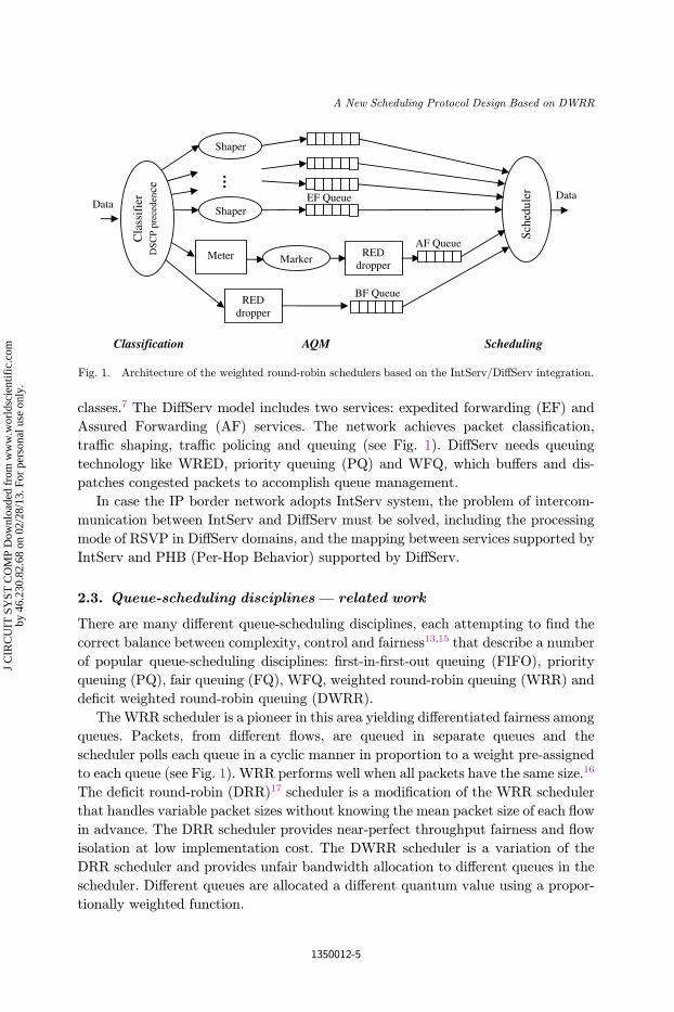
classes.7 The Di®Serv model includes two services: expedited forwarding (EF) and
Assured Forwarding (AF) services. The network achieves packet classi¯cation,
tra±c shaping, tra±c policing and queuing (see Fig. 1). Di®Serv needs queuing
technology like WRED, priority queuing (PQ) and WFQ, which bu®ers and dis-
patches congested packets to accomplish queue management.
In case the IP border network adopts IntServ system, the problem of intercom-
munication between IntServ and Di®Serv must be solved, including the processing
mode of RSVP in Di®Serv domains, and the mapping between services supported by
IntServ and PHB (Per-Hop Behavior) supported by Di®Serv.
2.3. Queue-scheduling disciplines — related work
There are many di®erent queue-scheduling disciplines, each attempting to ¯nd the
correct balance between complexity, control and fairness13,15 that describe a number
of popular queue-scheduling disciplines: ¯rst-in-¯rst-out queuing (FIFO), priority
queuing (PQ), fair queuing (FQ), WFQ, weighted round-robin queuing (WRR) and
de¯cit weighted round-robin queuing (DWRR).
The WRR scheduler is a pioneer in this area yielding di®erentiated fairness among
queues. Packets, from di®erent °ows, are queued in separate queues and the
scheduler polls each queue in a cyclic manner in proportion to a weight pre-assigned
to each queue (see Fig. 1). WRR performs well when all packets have the same size.16
The de¯cit round-robin (DRR)17 scheduler is a modi¯cation of the WRR scheduler
that handles variable packet sizes without knowing the mean packet size of each °ow
in advance. The DRR scheduler provides near-perfect throughput fairness and °ow
isolation at low implementation cost. The DWRR scheduler is a variation of the
DRR scheduler and provides unfair bandwidth allocation to di®erent queues in the
scheduler. Di®erent queues are allocated a di®erent quantum value using a propor-
tionally weighted function.
RED dropper
Shaper
Shaper
Meter RED dropper
Marker
…
Sche
dule
r
Data Data EF Queue
AF Queue
BF Queue
Cla
ssif
ier
DSC
P pr
eced
ence
Classification AQM Scheduling
Fig. 1. Architecture of the weighted round-robin schedulers based on the IntServ/Di®Serv integration.
A New Scheduling Protocol Design Based on DWRR
1350012-5
J C
IRC
UIT
SY
ST C
OM
P D
ownl
oade
d fr
om w
ww
.wor
ldsc
ient
ific
.com
by 4
6.23
0.82
.68
on 0
2/28
/13.
For
per
sona
l use
onl
y.
Recently, Ref. 7 proposed to apply IntServ model in Di®Serv-based EPON
(Ethernet passive optical network), which uses per-°ow processing to guarantee QoS.
A combined Di®Serv and IntServ model is employed in an EPON system, with a
dynamic bandwidth allocation algorithm to provide more °exible user-oriented
service quality. Later, Ref. 8 proposed new User-oriented Hierarchical bandwidth
Scheduling Algorithms (UHSAs) that support Di®Serv and guaranteed fairness
among end users.8 Includes inter and intra-optical network unit (ONU) scheduling
processes. The inter-ONU scheduling adopts an improved hybrid cycle approach that
separates a frame into a static part for high priority tra±c and an adaptive dynamic
part for low priority tra±c. The intra-ONU scheduling proposes credit-based
scheduling approach to guarantee fairness among end users.
For implementation bene¯ts and due to the °exible and scalable modular circuit
design approach, certain circuit architecture can be targeted for a full ASIC imple-
mentation. Thus, Ref. 2 proposed a full hardware implementation of a WFQ packet
scheduler in order to deliver 50Gb/s throughput. The circuit comprises three main
components; a WFQ algorithm computation circuit, a tag/time-stamp sort and re-
trieval circuit and a shared bu®er. However, the overall performance of the WFQ
circuit is limited by the technology available on the development board, particularly
the memory bus between the FPGA and the RLDRAM II.
This paper proposes a new scheduling technique, called Negative-DWRR, to meet
the DWRR limitations and improve the bandwidth utilization rate without in-
creasing the total latency. Then, a fully hardware packet scheduler is implemented
and veri¯ed as part of an intellectual property core.
3. Negative De¯cit Weighted Round-Robin Scheduler
In this section, we propose a new approach for a queue-scheduling discipline. This
approach, called Negative-de¯cit weighted round robin, is an extended technique
from the DWRR and WRR models.
3.1. WRR and DWRR limitations
WRR and DWRR models support °ows with signi¯cantly di®erent bandwidth
requirements. They ensure that lower-priority queues are not denied access to bu®er
space and output port bandwidth.13 However, WRR's inability to support the pre-
cise allocation of bandwidth when scheduling variable-length packets is a critical
limitation that needs to be addressed. In DWRR, several packets at the head of a
visited queue are not serviced and they would wait the next round robin only because
their sizes are slightly higher than the permitted byte number. Consequently, these
packets may be delayed before they can be serviced. The amount of delay, introduced
during a round needed for scheduling the other queues, causes QoS degradation. It
may cause the dropping of packets placed at the tail of the queue. Moreover, this
R. Ouni, J. Bhar & K. Torki
1350012-6
J C
IRC
UIT
SY
ST C
OM
P D
ownl
oade
d fr
om w
ww
.wor
ldsc
ient
ific
.com
by 4
6.23
0.82
.68
on 0
2/28
/13.
For
per
sona
l use
onl
y.
problem reduces packet throughput, increases end-to-end delay, causes jitter, and
can lead to packet loss if there is insu±cient bu®er memory to store all of the packets
that are waiting to be transmitted.
3.2. Negative DWRR parameters
The N-DWRR queue-scheduling discipline is proposed to address the limitations of
WRR and DWRR models and improve especially the bandwidth utilization rate
without increasing the total latency. It de¯nes new parameters that ¯rst allow in
supporting the weighted fair distribution of bandwidth when servicing queues that
contain variable-length packets. Secondly, they reduce the waiting delay for a packet
in a queue even if its size is large. This gives a precise allocation of bandwidth. In
N-DWRR queuing, each queue is con¯gured with the following parameters:
. A weight re°ects the importance of the service class routed over the queue. It
de¯nes the percentage of the output port bandwidth allocated to the queue. When
the weight of a queue is high, the number of bytes permitted for transmission is
high.
. A quantum of service is proportional to the weight of the queue and is expressed
in terms of bytes. Each round, the quantum is added to the number of bytes that a
queue can transmit.
. A credit is the number of bytes permitted for transmission but they are not yet
transmitted in the previous round. i.e., a queue that was not permitted to transmit
in the previous round, because the packet at the head of the queue was larger than
the value of the permitted bytes, could save transmission \credits" and use them
during the next service round.
. A negative credit is the number of bytes transmitted in the previous round over
the number of permitted bytes. The negative credit for a queue should not exceed
the sum of credits of all the queues.
. A de¯cit-counter speci¯es the total number of bytes that the queue is permitted
to transmit each time that it is visited by the scheduler. The De¯cit-Counter for a
queue is incremented by the quantum each time that the queue is visited by the
scheduler. It depends also on the values of the credit and the negative credit
parameters.
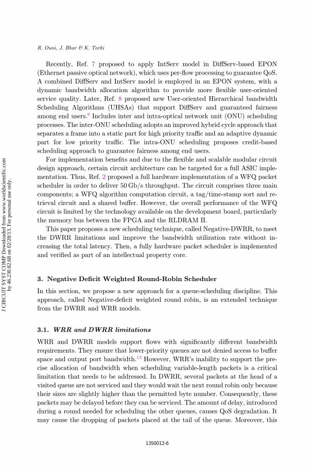
3.3. Negative DWRR algorithm
In the N-DWRR algorithm, the scheduler visits each nonempty queue and deter-
mines the number of bytes in the packet at the head of the queue. The de¯cit-counter
is variable and it takes, each round, a speci¯c value according to the quantum, the
credit and the negative-credit values. The de¯cit-counter is incremented by the value
A New Scheduling Protocol Design Based on DWRR
1350012-7
J C
IRC
UIT
SY
ST C
OM
P D
ownl
oade
d fr
om w
ww
.wor
ldsc
ient
ific
.com
by 4
6.23
0.82
.68
on 0
2/28
/13.
For
per
sona
l use
onl
y.
quantum. Two scenarios exist as a function of the size of the packet:
(1) If the size of the packet at the head of the queue is less than or equal to the
variable de¯cit-counter, the packet is transmitted on the output port. Then, the
variable de¯cit-counter is reduced by the number of bytes in the packet. The rest
of the subtraction is called credit. The scheduler continues to dequeue packets
and decrements the variable de¯cit-counter by the size of the transmitted packet
until either the size of the packet at the head of the queue is greater than the
variable de¯cit-counter or the queue is empty.
(2) If the size of the packet at the head of the queue is greater than the variable
de¯cit-counter, then one of the following two situations take place:
(a) If the size of the packet at the head of the queue is less than or equal to the
variable de¯cit-counter incremented by the available credits of all the queues,
the packet is transmitted on the output port. The negative-credit takes then
the value of the out of range transmitted bytes (of this packet) among the
available credit. The latter depends on credits and negative-credits of all
queues as explained in Fig. 2. The variable de¯cit-counter as well as the credit
are reset to zero. The scheduler moves on to service the next nonempty queue.
This situation can be explained by the fact that the current queue has taken
a part of the bandwidth unused by the other queues. In general, this part of
Queue (i)
Wi <= Weight queue(i) Qi <= Quantum queue(i) DCi <= Deficit counter queue(i)
Pckt_size <
DCi Transmit pckt DCi <= DCi – pckt_size
Pckt_size <
DCx Transmit pckt
N_credit = pckt_size - DCi
Credit <= reset (0)
DCi <= reset (0)
Queue (i+1) Credit <= DCi N_credit <= reset (0)
Yes
No
Yes
No
Wi ≡ traffic typeQi depends on Wi DCi = f ct (Qi, credit(i), n_credit(i))
• Av_credit = DCi * Beta-i (Available credits) • Adding Av_credit without exceeding total bandwidth
DCx <= DCi + Av_credit
next packet
Fig. 2. The N-DWRR algorithm state diagram.
R. Ouni, J. Bhar & K. Torki
1350012-8
J C
IRC
UIT
SY
ST C
OM
P D
ownl
oade
d fr
om w
ww
.wor
ldsc
ient
ific
.com
by 4
6.23
0.82
.68
on 0
2/28
/13.
For
per
sona
l use
onl
y.
bandwidth depends on (i) the credit and the negative credit of all queues and
(ii) the size of the packet at head of this queue. This portion of bandwidth
will be subtracted, at the next round, from the bandwidth allocated to this
queue. This approach allows reducing packet latency in queues, without
exceeding the total bandwidth.
(b) If the size of the packet at the head of the queue is greater than the variable
de¯cit-counter incremented by the sum of the credit of all the queues, the
scheduler moves on to service the next nonempty queue. This queue will be
characterized by two values (credit and negative-credit), which will be used
within the next visit (round). The credit takes the last value of the de¯cit-
counter. However, the negative-credit is reset to zero.
(3) When the queue is empty, the scheduler sets to zero the de¯cit-counter, the credit
and the negative-credit values and moves on to service the next nonempty queue.
Figure 2 shows the NDWRR algorithm. It presents two test levels before deciding to
transmit a packet or to move on to service the next nonempty queue. These two test
levels give more probability to transmit a packet and decrease the average queue size,
which avoids congestion of packets in the tail of each queue.
4. N-DWRR Performance Evaluation
A queue-scheduling discipline allows managing the access to a ¯xed amount of
output port bandwidth by selecting the next packet that is transmitted on a port.
The packet transmission order depends on two parameters: the bandwidth allocated
to each queue (weight Wi) and Beta. Beta is a new parameter introduced by
N-DWRR to improve the total bandwidth utilization. It represents an additional
amount of bandwidth to o®er for each queue from the unused band. Our approach
provides a limited band without exceeding the total bandwidth. N-DWRR assumes
that the total bandwidth is not in general fully occupied. Therefore, the free band can
be distributed according to the needs of all queues.
4.1. Simulation environment and parameters
In this section, using Opnet modeler, we evaluate the performance of the most popular
scheduling techniques, at di®erent scenarios, based on many service classes: VoIP,
FTP, HTTP and Email. We consider a topology/network architecture including
mainly two parts: network core and network edge. In total, this environment includes
112 hardware devices (routers, switches, workstations, servers and VoIP telephones),
115 physical link (serial, Ethernet) and 3 con¯guration utilities. The simulation
scenario is based on many communication features such as tra±c type, number of
sources, tra±c starting time, tra±c data rate, etc. Each simulation scenario is done
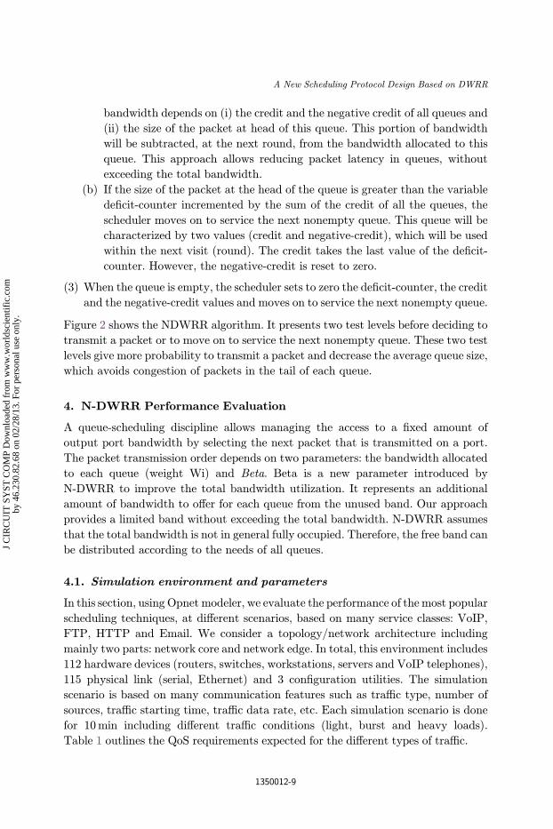
for 10min including di®erent tra±c conditions (light, burst and heavy loads).
Table 1 outlines the QoS requirements expected for the di®erent types of tra±c.
A New Scheduling Protocol Design Based on DWRR
1350012-9
J C
IRC
UIT
SY
ST C
OM
P D
ownl
oade
d fr
om w
ww
.wor
ldsc
ient
ific
.com
by 4
6.23
0.82
.68
on 0
2/28
/13.
For
per
sona
l use
onl
y.
4.2. Simulation results
In order to evaluate the performance of the proposed technique, two simulation levels
are suggested. First, the simulation of the most popular scheduling techniques
deployed for Di®Serv in IP networks is done. This allows selecting the most e®ective
technique in terms of bandwidth utilization and latency. Second, using computer
simulation, we evaluate the performance of the proposed N-DWRR algorithm
compared to the selected technique.
4.2.1. Popular scheduling algorithms evaluation
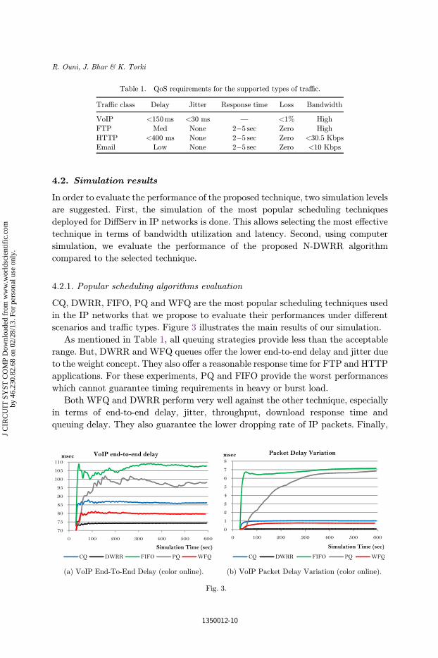
CQ, DWRR, FIFO, PQ and WFQ are the most popular scheduling techniques used
in the IP networks that we propose to evaluate their performances under di®erent
scenarios and tra±c types. Figure 3 illustrates the main results of our simulation.
As mentioned in Table 1, all queuing strategies provide less than the acceptable
range. But, DWRR and WFQ queues o®er the lower end-to-end delay and jitter due
to the weight concept. They also o®er a reasonable response time for FTP and HTTP
applications. For these experiments, PQ and FIFO provide the worst performances
which cannot guarantee timing requirements in heavy or burst load.
Both WFQ and DWRR perform very well against the other technique, especially
in terms of end-to-end delay, jitter, throughput, download response time and
queuing delay. They also guarantee the lower dropping rate of IP packets. Finally,
Table 1. QoS requirements for the supported types of tra±c.
Tra±c class Delay Jitter Response time Loss Bandwidth
VoIP <150ms <30 ms — <1% High
FTP Med None 2�5 sec Zero High
HTTP <400 ms None 2�5 sec Zero <30.5 KbpsEmail Low None 2�5 sec Zero <10 Kbps
(a) VoIP End-To-End Delay (color online). (b) VoIP Packet Delay Variation (color online).
Fig. 3.
R. Ouni, J. Bhar & K. Torki
1350012-10
J C
IRC
UIT
SY
ST C
OM
P D
ownl
oade
d fr
om w
ww
.wor
ldsc
ient
ific
.com
by 4
6.23
0.82
.68
on 0
2/28
/13.
For
per
sona
l use
onl
y.
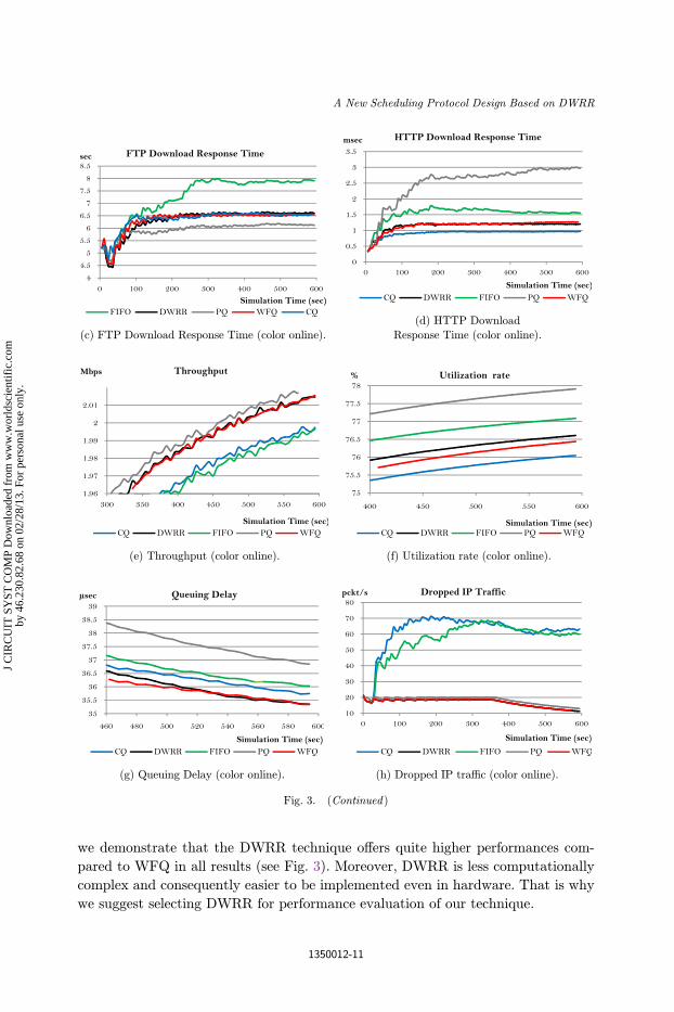
we demonstrate that the DWRR technique o®ers quite higher performances com-
pared to WFQ in all results (see Fig. 3). Moreover, DWRR is less computationally
complex and consequently easier to be implemented even in hardware. That is why
we suggest selecting DWRR for performance evaluation of our technique.
(c) FTP Download Response Time (color online).
(d) HTTP Download
Response Time (color online).
(e) Throughput (color online). (f) Utilization rate (color online).
(g) Queuing Delay (color online). (h) Dropped IP tra±c (color online).
Fig. 3. (Continued )
A New Scheduling Protocol Design Based on DWRR
1350012-11
J C
IRC
UIT
SY
ST C
OM
P D
ownl
oade
d fr
om w
ww
.wor
ldsc
ient
ific
.com
by 4
6.23
0.82
.68
on 0
2/28
/13.
For
per
sona
l use
onl
y.
4.2.2. Bandwidth utilization
In this section, we evaluate the performance of the proposed N-DWRR technique
through extensive simulation experiments maintained within a single IP router based
on a scalable architecture of queues. Here, four queues having di®erent weights are
deployed to store IP packets which are delivered randomly with variable size and
support di®erent types of tra±c. For the purpose of comparison and to show the
provided advantages, the performance evaluation consists mainly of measuring two
QoS metrics: the bandwidth utilization rate and latency. The ¯rst metric measures
the total bandwidth used by all queues during each round. The latency measures the
total queuing delay of all packets of the same weight.
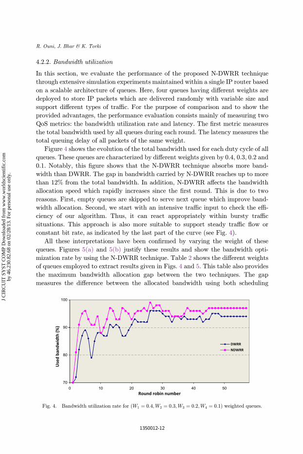
Figure 4 shows the evolution of the total bandwidth used for each duty cycle of all
queues. These queues are characterized by di®erent weights given by 0.4, 0.3, 0.2 and
0.1. Notably, this ¯gure shows that the N-DWRR technique absorbs more band-
width than DWRR. The gap in bandwidth carried by N-DWRR reaches up to more
than 12% from the total bandwidth. In addition, N-DWRR a®ects the bandwidth
allocation speed which rapidly increases since the ¯rst round. This is due to two
reasons. First, empty queues are skipped to serve next queue which improve band-
width allocation. Second, we start with an intensive tra±c input to check the e±-
ciency of our algorithm. Thus, it can react appropriately within bursty tra±c
situations. This approach is also more suitable to support steady tra±c °ow or
constant bit rate, as indicated by the last part of the curve (see Fig. 4).
All these interpretations have been con¯rmed by varying the weight of these
queues. Figures 5(a) and 5(b) justify these results and show the bandwidth opti-
mization rate by using the N-DWRR technique. Table 2 shows the di®erent weights
of queues employed to extract results given in Figs. 4 and 5. This table also provides
the maximum bandwidth allocation gap between the two techniques. The gap
measures the di®erence between the allocated bandwidth using both scheduling
70
80
90
100
0 10 20 30 40 50
Use
d ba
ndw
idth
(%)
Round robin number
DWRR
NDWRR
Fig. 4. Bandwidth utilization rate for (W1 ¼ 0:4;W2 ¼ 0:3;W3 ¼ 0:2;W4 ¼ 0:1) weighted queues.
R. Ouni, J. Bhar & K. Torki
1350012-12
J C
IRC
UIT
SY
ST C
OM
P D
ownl
oade
d fr
om w
ww
.wor
ldsc
ient
ific
.com
by 4
6.23
0.82
.68
on 0
2/28
/13.
For
per
sona
l use
onl
y.
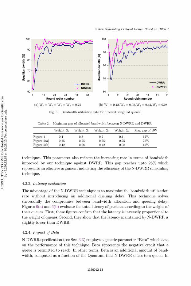
techniques. This parameter also re°ects the increasing rate in terms of bandwidth
improved by our technique against DWRR. This gap reaches upto 25% which
represents an e®ective argument indicating the e±ciency of the N-DWRR scheduling
technique.
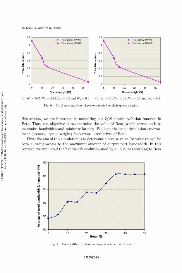
4.2.3. Latency evaluation
The advantage of the N-DWRR technique is to maximize the bandwidth utilization
rate without introducing an additional queuing delay. This technique solves
successfully the compromise between bandwidth allocation and queuing delay.
Figures 6(a) and 6(b) evaluate the total latency of packets according to the weight of
their queues. First, these ¯gures con¯rm that the latency is inversely proportional to
the weight of queues. Second, they show that the latency maintained by N-DWRR is
slightly lower than DWRR.
4.2.4. Impact of Beta
N-DWRR speci¯cation (see Sec. 3.3) employs a generic parameter \Beta" which acts
on the performance of this technique. Beta represents the negative credit that a
queue is permitted to reach. In other terms, Beta is an additional amount of band-
width, computed as a fraction of the Quantum that N-DWRR o®ers to a queue. In
Table 2. Maximum gap of allocated bandwidth between N-DWRR and DWRR.
Weight Q1 Weight Q2 Weight Q3 Weight Q4 Max gap of BW
Figure 4 0.4 0.3 0.2 0.1 12%
Figure 5(a) 0.25 0.25 0.25 0.25 25%Figure 5(b) 0.42 0.08 0.42 0.08 15%
50
60
70
80
90
100
DWRRNDWRR
(a) W1 ¼ W2 ¼ W3 ¼ W4 ¼ 0:25
60
70
80
90
100
DWRR
NDWRR
(b) W1 ¼ 0:42;W2 ¼ 0:08;W3 ¼ 0:42;W4 ¼ 0:08
Fig. 5. Bandwidth utilization rate for di®erent weighted queues.
A New Scheduling Protocol Design Based on DWRR
1350012-13
J C
IRC
UIT
SY
ST C
OM
P D
ownl
oade
d fr
om w
ww
.wor
ldsc
ient
ific
.com
by 4
6.23
0.82
.68
on 0
2/28
/13.
For
per
sona
l use
onl
y.
this section, we are interested in measuring our QoS metric evolution function in
Beta. Thus, the objective is to determine the value of Beta, which serves both to
maximize bandwidth and minimize latency. We kept the same simulation environ-
ment (scenario, queue weight) for various alternatives of Beta.
First, the aim of this simulation is to determine a precise value (or value range) for
beta allowing access to the maximum amount of output port bandwidth. In this
context, we simulated the bandwidth evolution used by all queues according to Beta
0
0.2
0.4
0.6
0.8
1
1.2
5 15 25 35 45 55
Tota
llat
ency
(ms)
Queue weight (%)
Total latency (DWRR)
Total latency (NDWRR)
(a) W1 ¼ 0:05;W2 ¼ 0:15;W3 ¼ 0:2 and W4 ¼ 0:6
0
0.2
0.4
0.6
0.8
1
1.2
5 15 25 35 45 55
Tota
llat
ency
(ms)
Queue weight (%)
Total latency (DWRR)
Total latency (NDWRR)
(b) W1 ¼ 0:1;W2 ¼ 0:2;W3 ¼ 0:3 and W4 ¼ 0:4
Fig. 6. Total queuing delay of packets related to their queue weights.
90
91
92
93
94
95
5 15 25 35 45 55
Ave
rage
of u
sed
band
wid
th (a
ll qu
eues
) (%
)
Beta (%)
Fig. 7. Bandwidth utilization average as a function of Beta.
R. Ouni, J. Bhar & K. Torki
1350012-14
J C
IRC
UIT
SY
ST C
OM
P D
ownl
oade
d fr
om w
ww
.wor
ldsc
ient
ific
.com
by 4
6.23
0.82
.68
on 0
2/28
/13.
For
per
sona
l use
onl
y.
variation. In Fig. 7, the result shows that the used bandwidth increases with Beta to
reach a peak near the range of 35�45%. The bandwidth decreases slightly beyond the
peak value and then keeps almost constant. However, the queuing delay becomes
particularly high (see Fig. 8). Therefore, the choice of Beta should satisfy the com-
promise between bandwidth allocation and queuing delay.
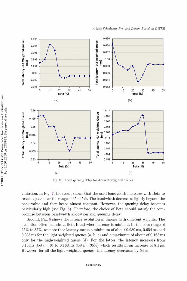
Second, Fig. 8 shows the latency evolution in queues with di®erent weights. The
evolution often includes a Beta Band where latency is minimal. In the beta range of
25% to 35%, we note that latency meets a minimum of about 0.989ms, 0.654ms and
0.335ms for the light weighted queues (a, b, c) and a maximum of about of 0.168ms
only for the high-weighted queue (d). For the latter, the latency increases from
0.16ms (beta ¼ 0) to 0.168ms (beta ¼ 35%) which results in an increase of 8.1�s.
However, for all the light weighted queues, the latency decreases by 54�s.
0.988
0.989
0.99
0.991
0.992
0.993
0.994
0.995
(a)
0.652
0.654
0.656
0.658
0.66
0.662
0.664
0.666
(b)
0.33
0.335
0.34
0.345
0.35
0.355
0.36
(c)
0.152
0.154
0.156
0.158
0.16
0.162
0.164
0.166
0.168
0.17
(d)
Fig. 8. Total queuing delay for di®erent weighted queues.
A New Scheduling Protocol Design Based on DWRR
1350012-15
J C
IRC
UIT
SY
ST C
OM
P D
ownl
oade
d fr
om w
ww
.wor
ldsc
ient
ific
.com
by 4
6.23
0.82
.68
on 0
2/28
/13.
For
per
sona
l use
onl
y.
In conclusion, the common Beta range providing optimized values is limited be-
tween 25% and 35%. We choose Beta equal to 30% in order to obtain optimal results
which are already outlined in Secs. 4.2.2 and 4.2.3.
5. RTL Design of Embedded Packet Processors
Until recently, such a router used to be implemented entirely in software, running on
a general-purpose processor in a host computer. However, such implementations are
increasingly becoming infeasible because of two reasons: performance requirements
and complexity of the packet-processing functions. During the last few years, the
available network bandwidth has been on the rise, and with the advent of optical
¯bers being deployed for networking, network bandwidth has increased exponen-
tially. This has led to very stringent performance requirements from routers since
they have to process packets at line speed. Further, any new service to be supported
by a network is implemented by extending or modifying the routers. This has led to
very complex functionality being built in routers, with the additional requirement of
being reasonably °exible.
The real-time packet-processing constraints imposed on routers to support high-
line speeds motivate hardware-based solutions, where the router functionality is
implemented on application speci¯c integrated circuits (ASICs). The requirements
for °exibility and the complex nature of many of the processing functions, on the
other hand, favor software-based implementations on general-purpose processors. To
address these two con°icting issues, recently a new class of devices called \network
processors" has emerged.18 These are high performance programmable devices with
special architectural features that are optimized for packet processing. It is moti-
vated by the fact that the design and analysis of hardware�software architectures
for such processors requires new models and methods, which do not fall under the
domain of traditional embedded systems design.19,20
5.1. RTL design: Issues and trends
Most of today's embedded systems are implemented as a system-on-chip (SoC). In
the context of network packet processors, the architecture of such systems consists of
a heterogeneous combination of di®erent hardware and software components. The
hardware components consist of dedicated hardware block cores, di®erent kinds of
memory modules and caches, various interconnections and input�output inter-
faces.21 All of these are integrated on a single chip and run specialized software to
perform packet processing. The process of determining the optimal hardware and
software architecture for such processors includes issues involving resource alloca-
tion, partitioning and design space exploration. To tackle the complexity of such
designs, and also to meet demands for short time-to-market and low cost, several new
design paradigms like platform-based design19 have evolved. These are based on the
R. Ouni, J. Bhar & K. Torki
1350012-16
J C
IRC
UIT
SY
ST C
OM
P D
ownl
oade
d fr
om w
ww
.wor
ldsc
ient
ific
.com
by 4
6.23
0.82
.68
on 0
2/28
/13.
For
per
sona
l use
onl
y.
idea of concurrent design of hardware and software, and the design °ow starts with
an abstract speci¯cation of the application.
According to a protocol stack architecture, routers are built especially over two
layers, MAC in layer-2 and IP in layer-3. Forwarding frames are based on layer-2
MAC address information. Because of the standardization of the IP as the layer-3
protocol in local- and wide-area networks, layer-3 switching made it possible to do
classi¯cation and forwarding of packets based on their layer-3 DSCP ¯eld, without
resorting to complex routing algorithms. Since IP packets make up the major portion
of tra±c in any switch or router, we o®er here a solution where IP classi¯cation,
discarding, queuing, scheduling and forwarding were hardwired into ASICs.
5.2. Logic synthesis
Logic synthesis is one of the most important phases of the design °ow in state-of-the-
art circuits. It aims at transforming the HDL (usually Verilog HDL or VHDL)
description of the circuit into a technology-dependent, gate-level netlist. Through
this process, the hardware designer de¯nes the environmental conditions, con-
straints, compile methodology, design rules and target libraries, in order to achieve
certain design goals set by the initial speci¯cations. The tool we use for the logic
synthesis of the circuit is Synopsys DC, the most widely used synthesis tool. DC
optimizes logic designs for speed, area and wire routability. From the de¯ned goals,
DC synthesizes the circuit and tailors it to a target technology. The gate-level re-
presentation of the circuit is the input ¯le to the Place and Route tool.
The synthesis process is completed relatively easily and timing constraints are
met, while circuit area is kept to a minimum. Timing constraints are of the greatest
importance, as we opted for a clock frequency of 300MHz (3.33 ns clock cycle). We
were constrained to 300MHz due to the fact that it was the maximum operating
frequency of the FIFO we had. The circuit integrates 12 FIFOs as queues needed for
multiple port reception, di®erentiated service classi¯cation and scheduling. Hence,
we achieve 76.8Gbit/s incoming router throughput (8 inputs of 9.6Gbit/s link
throughput). Synthesis results are given in Table 3.
5.3. Post-synthesis veri¯cation
Post-synthesis veri¯cation is possibly the most important phase of the synthesis °ow.
It aims at testing whether the initial RTL design has the same behavior as the gate-
level netlist produced by the synthesis tool. In most cases, the initial results are not
the same, and the designer has to carefully investigate the reasons for the erroneous
behavior of the gate-level netlist. Usual mistakes happen when the circuit does not
reset correctly, a mistake that can pass unseen from the HDL compiler and simu-
lator, but, of course, the actual circuit will not work correctly.
Our synthesized gate-level netlist is imported back to the gate-level DC and is
tested within the same environment as the initial RTL design. The ¯nal netlist
A New Scheduling Protocol Design Based on DWRR
1350012-17
J C
IRC
UIT
SY
ST C
OM
P D
ownl
oade
d fr
om w
ww
.wor
ldsc
ient
ific
.com
by 4
6.23
0.82
.68
on 0
2/28
/13.
For
per
sona
l use
onl
y.
proved to behave correctly. The netlist is now ready to be imported to the Place &
Route tool for the ¯nal phase of the design process.
5.4. Place and route °ow
We place and route (P&R) the router chip core with Cadence Encounter.22 It is
comprised of various stages, some of them being optional, although important for
new design cases. At ¯rst, the design is imported to the tool. The ¯les needed are
technology-dependent and are either given by the technology vendor (in our case
CMOS 0.35�m) or are produced by the synthesis tool (in our case Synopsys Design
Compiler). The vendor provides the P&R tool with (a) technology library (.lib ¯les),
which contains the exact electrical characteristics of the library standard cells, (b)
layout (.lef ¯les), which includes standard cell actual layout, pin placement and
metal layer usage and (c) verilog (.v ¯les), containing the interface of every standard
cell. The same vendor also provides the memory models speci¯ed by their timing
library (.tlf ¯les). From the synthesis tool point of view, the only information needed
to be passed on to the P&R tool is the Synopsys technology mapped (.v) gate-level
representation of the design.
After importing the design, the designer has to °oorplan the various HDL mod-
ules and/or black boxes in the actual chip. Power rings are created and block rings
are added for power/ground termination purposes. Input/Output pins are also
placed in this stage. The most important decisions are, of course, exact chip layout,
utilization percentage and I/O placement.
When trial routing is complete, we move to the Clock Tree Placement phase. This
is achieved with bu®er insertions and thorough computations of the tree node
weights, so as to minimize clock skew produced by unbalanced clock tree placement.
In the ¯nal route phase, setup and hold times of registers are taken into account and,
having in mind the operating frequency constraint, the tools try to bu®er wires and
resize standard cells in order to minimize clock skew.
5.5. P&R results
The classi¯er, AQM and scheduler chip we place and route has a total area of
88.72mm2, with a square shape of (9:4� 9:4mm), as presented in Fig. 9. Area
results, as well as gate number can be seen in Table 4.
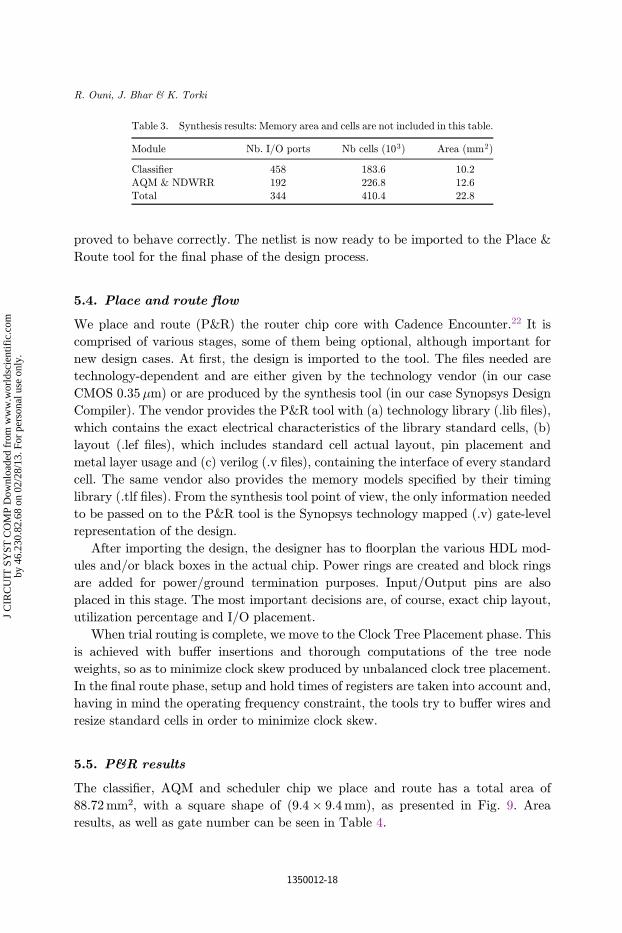
Table 3. Synthesis results: Memory area and cells are not included in this table.
Module Nb. I/O ports Nb cells (103) Area (mm2)
Classi¯er 458 183.6 10.2
AQM & NDWRR 192 226.8 12.6Total 344 410.4 22.8
R. Ouni, J. Bhar & K. Torki
1350012-18
J C
IRC
UIT
SY
ST C
OM
P D
ownl
oade
d fr
om w
ww
.wor
ldsc
ient
ific
.com
by 4
6.23
0.82
.68
on 0
2/28
/13.
For
per
sona
l use
onl
y.
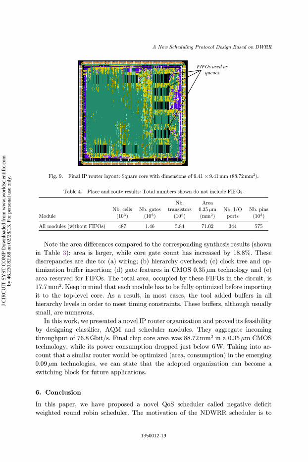
Note the area di®erences compared to the corresponding synthesis results (shown
in Table 3): area is larger, while core gate count has increased by 18.8%. These
discrepancies are due to: (a) wiring; (b) hierarchy overhead; (c) clock tree and op-
timization bu®er insertion; (d) gate features in CMOS 0.35�m technology and (e)
area reserved for FIFOs. The total area, occupied by these FIFOs in the circuit, is
17.7mm2. Keep in mind that each module has to be fully optimized before importing
it to the top-level core. As a result, in most cases, the tool added bu®ers in all
hierarchy levels in order to meet timing constraints. These bu®ers, although usually
small, are numerous.
In this work, we presented a novel IP router organization and proved its feasibility
by designing classi¯er, AQM and scheduler modules. They aggregate incoming
throughput of 76.8Gbit/s. Final chip core area was 88.72mm2 in a 0.35�m CMOS
technology, while its power consumption dropped just below 6W. Taking into ac-
count that a similar router would be optimized (area, consumption) in the emerging
0.09�m technologies, we can state that the adopted organization can become a
switching block for future applications.
6. Conclusion
In this paper, we have proposed a novel QoS scheduler called negative de¯cit
weighted round robin scheduler. The motivation of the NDWRR scheduler is to
Table 4. Place and route results: Total numbers shown do not include FIFOs.
Module
Nb. cells
(103)
Nb. gates
(106)
Nb.
transistors
(106)
Area
0.35�m
(mm2)
Nb. I/O
ports
Nb. pins
(103)
All modules (without FIFOs) 487 1.46 5.84 71.02 344 575
FIFOs used as queues
Fig. 9. Final IP router layout: Square core with dimensions of 9:41� 9:41mm (88.72mm2).
A New Scheduling Protocol Design Based on DWRR
1350012-19
J C
IRC
UIT
SY
ST C
OM
P D
ownl
oade
d fr
om w
ww
.wor
ldsc
ient
ific
.com
by 4
6.23
0.82
.68
on 0
2/28
/13.
For
per
sona
l use
onl
y.
provide end-to-end bandwidth guarantees for di®erentiated service classes in large IP
networks. It can maintain its weighted share of bandwidth and provide delay dif-
ferentiation among queues. However, this is done at the cost of a higher algorithmic
complexity due to the rearrangement of service order according to the weight of the
packets at the head of each queue.
The N-DWRR scheduler provides two advantages. First, it works with variable
size packets. Second, the N-DWRR scheduler avoids having a packet waiting in
queue only because its size is slightly higher than the variable de¯cit-counter. This
problem occurs in the DWRR scheduler. However, in the N-DWRR scheduler the
packet in the head of the queue can be transmitted, even there is no su±cient
bandwidth, without exceeding the total bandwidth of the network. In conclusion, the
N-DWRR scheduler provides its queues with delay di®erentiation in terms of average
and worst-case packet delay that is statistically less than the DWRR scheduler; and
with throughput fairness that is higher than the DWRR and WFQ schedulers.
Further, this work includes the design evaluation for an optimal architecture of
network processors. It introduces a new service scheme motivated by the require-
ments of multi-service access networks. Based on the synthesis and P&R steps, we
then evaluated di®erent combinations of algorithms (for policing, queuing and link
scheduling) along with di®erent hardware building blocks and memory architectures,
for the design of a packet processor to support the proposed service scheme.
Acknowledgments
This work is supported by the Research Center of the College of Computer and
Information Sciences — King Saud University.
References
1. P. Giacomazzi, L. Musumeci, G. Saddemi and G. Verticale, Two di®erent approaches forproviding QoS in the Internet backbone, Comput. Commun. 29 (2006) 3957�3969.
2. K. McLaughlin, D. Burns, C. Toal, C. McKillen and S. Sezer, Fully hardware based WFQarchitecture for high-speed QoS packet scheduling, Integration VLSI J. (2011),doi:10.1016/j.vlsi.2011.01.001.
3. T. M. Lim, B. S. Lee and C. K. Yeo, Weighted de¯cit earliest departure ¯rst scheduling,Comput. Commun. 28 (2005) 1711�1720.
4. R. Braden, D. Clark and S. Shenker, Integrated services in the internet architecture: Anoverview, RFC (1633).
5. S. Blakem, D. Black, M. Carlson, E. Davies, Z. Wang and W. Weiss, An architecture fordi®erentiated service, RFC (2475).
6. S. Ece (Guran) Schmidt and H. S. Kim, Frame-counter scheduler: A novel QoS schedulerfor real-time tra±c, Comput. Commun. 29 (2006) 2181�2200.
7. L. Qiong, L. Hui, J. Yue-Feng and Q. Yao-Jun, Resources allocation in an Intserv/Di®serv integrated EPON system, J. China Univ. Posts Telecommunications 16 (2009)108�113.
R. Ouni, J. Bhar & K. Torki
1350012-20
J C
IRC
UIT
SY
ST C
OM
P D
ownl
oade
d fr
om w
ww
.wor
ldsc
ient
ific
.com
by 4
6.23
0.82
.68
on 0
2/28
/13.
For
per
sona
l use
onl
y.
8. Y. Yin and G. Poo, User-oriented hierarchical bandwidth scheduling for Ethernet passiveoptical networks, Comput. Commun. 33 (2010) 965�975.
9. S. Floyd and V. Jacobson, Random early detection gateways for congestion avoidance,IEEE/ACM Trans. Netw. 1 (1993) 397�413.
10. M. Wurtzler, Analysis and simulation of weighted random early detection (WRED)queues, EECS 891 project, 2002.
11. S. Mishima, L. Moy-Yee, G. Yee-Madera and E. Youse¯, Broadband packet switchprocessor, Space Commun. 18 (2002) 91�95.
12. Y. Mo, J. M. Nho, Yang, N. P. Mahalik, K. Kim and B. H. Ahn, A tra±c-class burst-polling based delta DBA scheme for QoS in distributed EPONs, Comput. Stand. Interfac.28 (2006) 721�736.
13. Supporting di®erentiated service classes: Queue scheduling disciplines, white paper chucksemeria, marketing engineer. Part number 200020-001, December 2001.
14. J. Postel, Internet protocol, DARPA Internet program protocol speci¯cation RFC791,September 1981.
15. L. Le, J. Aikat, K. Je®ay and F. D. Smith, The e®ects of active queue management on webperformance, in SIGCOMM'03, Germany, 25�29 August 2003, pp. 265�276.
16. M. Y. L. Wong and C. K. Li, Low computational complexity weighted queuing usingweighted De¯cit Round Robin, Proc. IASTED Application Information, Innsbruck,Austria (2002).
17. M. Shreedhar and G. Varghese, E±cient fair queuing using De¯cit Round Robin, IEEE/ACM Trans. Netw. 4 (1996) 375�385.
18. S. Chakraborty, System-level timing analysis and scheduling for embedded packet pro-cessors, Thesis of the Swiss Federal Institute of Technology, Zurich, April 2003.
19. K. Keutzer, S. Malik, R. Newton, J. M. Rabaey and A. Sangiovanni-Vincentelli, Systemlevel design: Orthogonolization of concerns and platform-based design, IEEE Trans.Comput.-Aided Des. 19 (2000).
20. R. A. Bergamaschi, S. Bhattacharya, R. Wagner, C. Fellenz, M. Muhlada, W. R. Lee,F. White and J.-M. Daveau, Automating the design of SoCs using cores, IEEE Des. TestComput. 18 (2001) 32�45.
21. D. G. Simos, Design of a 32� 32 variable-packet-size bu®ered crossbar switch chip,Thesis of institute of computer science FORTH-ICS/TR-339, July 2004.
22. Cadence Corporation; Available at http://www.cadence.com.
A New Scheduling Protocol Design Based on DWRR
1350012-21
J C
IRC
UIT
SY
ST C
OM
P D
ownl
oade
d fr
om w
ww
.wor
ldsc
ient
ific
.com
by 4
6.23
0.82
.68
on 0
2/28
/13.
For
per
sona
l use
onl
y.
This article appeared in a journal published by Elsevier. The attachedcopy is furnished to the author for internal non-commercial researchand education use, including for instruction at the authors institution
and sharing with colleagues.
Other uses, including reproduction and distribution, or selling orlicensing copies, or posting to personal, institutional or third party
websites are prohibited.
In most cases authors are permitted to post their version of thearticle (e.g. in Word or Tex form) to their personal website orinstitutional repository. Authors requiring further information
regarding Elsevier’s archiving and manuscript policies areencouraged to visit:
http://www.elsevier.com/copyright
Author's personal copy
Dynamic slot assignment protocol for QoS support on TDMA-based mobile networks
Ridha Ouni ⁎College of Computer and Information Sciences, King Saud University, Kingdom of Saudi ArabiaFaculty of Sciences of Monastir, EμE, Tunisia
a b s t r a c ta r t i c l e i n f o
Article history:Received 2 November 2009Received in revised form 21 May 2011Accepted 15 June 2011Available online 2 July 2011
Keywords:TDMA/FDDWLANBandwidth allocationQoSMAC protocol
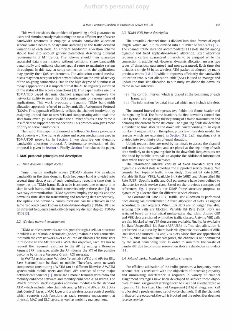
An efficient bandwidth allocation scheme in wireless networks should not only guarantee successful datatransmission without collisions but also enhance the channel spatial reuse to maximize the systemthroughput. The design of high-performance wireless Local Area Network (LAN) technologies making use ofTDMA/FDD MAC (Time Division Multiple Access/Frequency Division Duplex – Medium Access Control) is avery active area of research and development. Several protocols have been proposed in the literature asTDMA-based bandwidth allocation schemes. However, they do not have a convenient generic parameters orsuitable frame repartition for dynamic adjustment. In this work, we undertake the design and performanceevaluation of a QoS (Quality of Service)-aware scheme built on top of the underlying signaling and bandwidthallocation mechanisms provided by most wireless LANs standards. The main contribution of this study is thenew guarantee-based dynamic adjustment algorithm used in MAC level to provide the required QoS for alltraffic types in wireless medium especially Wireless ATM (Asynchronous Transfer Mode). Performanceevaluation of this approach consists of improving the bandwidth utilization, supporting different QoSrequirements and reducing call reject probability and packet latency.
© 2011 Elsevier B.V. All rights reserved.
1. Introduction
Several wireless networking solutions have been developed toprovide different types of services for various end user applications.Wireless mobile data communication has been enlarged with thedevelopments of high performance wireless computers and othermobile devices [1]. Bandwidth is a scarce resource that can be sharedeither dynamically according to the amount of data required to betransferred to or from each node or deterministically by assigning afixed number of slots to each cell, as in a cellular network [2]. With thedeterministic assignment, a fixed number of slots, as portion of thebandwidth, is assigned to certain nodes (or groups of nodes) so thatthey have exclusive access to the assigned bandwidth. The dynamicassignment shares the bandwidth into the required number of slotswhich can be changed according to the occurred events in thenetwork. Thus, a QoS (bandwidth, delay, jitter) guarantee can beprovided. However, traditional bandwidth allocation is pre-planned,hence, it is less adaptive to traffic load variations and networktopology changes [2].
Recently, several high-performance wireless LAN technologiesmaking use of TDMA/TDD (Time Division Duplex) MAC have beendesigned [3–5]. In this type of networks, a central unit allocates thebandwidth among all active mobile terminals. These lasts use a set of
signaling primitives in order to place their resource requests. Thecentral unit then allocates the channel bandwidth among all thecompeting mobiles [3].
TDMA/FDD (Frequency Division Duplex) MAC protocol is used toseparate uplink and downlink channels which are divided into acontiguous series of fixed-size TDMA frames. Each frame is furthersubdivided onto a fixed number of slots to be allocated for differentservice classes. TDMA wireless networks, when operating under theinfrastructure mode, distinguish between two types of devices: theAccess Point (AP) and the Mobile Terminal (MT) [3]. The AP is theentity responsible of providing connectivity with the core network aswell as for adapting the users’ requirements by taking into account thecharacteristics of the core network and the services offered by thewireless LAN. Furthermore, the AP distributes resources and main-tains coordination between all the MTs located within the cell [3].
Traditional wireless networks deployed universally cannot pro-vide the necessary QoS guarantees for bursty traffic such as real-timemultimedia applications [1]. Based on the MAC protocol, it is possibleto build up QoS mechanisms capable of providing the guaranteesneeded by various applications. Thesemechanisms need to specify theformat and sequence of the control messages between MTs and AP.However, they don’t define the specifics regarding the timing andnumerical values of the system parameters, such as the bandwidth tobe reserved for each type of connection [3]. In other hand, thesemechanisms may consider distributed dynamic slot and powerallocation for a TD/SDMA broadband wireless packet network withmultiple access ports and adaptive antennas [6].
Computer Standards & Interfaces 34 (2012) 146–155
⁎ CCIS, King Saud University, P.O. Box 51178, Riyadh 11543, Kingdom of Saudi Arabia.Fax: +966 1 4675630.
E-mail address: [email protected].
0920-5489/$ – see front matter © 2011 Elsevier B.V. All rights reserved.doi:10.1016/j.csi.2011.06.003
Contents lists available at ScienceDirect
Computer Standards & Interfaces
j ourna l homepage: www.e lsev ie r.com/ locate /cs i
Author's personal copy
This work considers the problem of providing a QoS guarantee tousers and simultaneously maintaining the most efficient use of scarcebandwidth resources. It employs a certain bandwidth allocationscheme which needs to be dynamic according to the traffic demandvariations at each node. An efficient bandwidth allocation schemeshould take into account generic parameters describing differentrequirements of MT traffics. This scheme should then guaranteesuccessful data transmissions without collisions, share bandwidthdynamically and enhance channel spatial reuse to maximize systemthroughput. In this way, at setup connection time, the applicationsmay specify their QoS requirements. The admission control mecha-nismsmay then accept or reject new calls based on the level of activityof the on-going connections. Due to the high degree of burstiness oftoday’s applications, it is important that the AP be regularly informedof the status of the active connections [3]. This paper makes use of aTDMA/FDD based dynamic channel assignment to improve thenetwork’s ability to meet the QoS requirements of various types ofapplications. This work proposes a dynamic TDMA bandwidthallocation approach referred to as Dynamic Slot Assignment Protocol(DSAP). This approach efficiently utilizes the channel bandwidth byassigning unused slots to newMTs and compensating additional timeslots from lower QoS classes when the number of slots in the frame isinsufficient to support new connections. This protocol also gives morepriority to serve handoff calls.
The rest of this paper is organized as follows. Section 2 provides ashort overview of the frame structure and access mechanisms used inTDMA/FDD networks. In Section 3, we describe our dynamicbandwidth allocation proposal. A performance evaluation of thisproposal is given in Section 4. Finally, Section 5 concludes the paper.
2. MAC protocol: principles and description
2.1. Time division multiple access
Time division multiple access (TDMA) shares the availablebandwidth in the time domain. Each frequency band is divided intoseveral time slots. A set of such periodically repeating time slots isknown as the TDMA frame. Each node is assigned one or more timeslots in each frame, and the node transmits only in those slots [3]. Fortwo-way communication, TDMA systems employ the uplink and thedownlink time slots for transmitting and receiving data respectively.The uplink and downlink communications can be achieved in thesame frequency band, known as time division duplex (TDMA/TDD), oron different frequency band, called frequency division duplex (TDMA-FDD) [2].
2.2. Wireless network environment
TDMAwireless networks are designed through a cellular structurein which a set of mobile terminals (nodes) maintain their connectiv-ities with the core network over an AP. the AP allocates the time slotsin response to the MT requests. With this objective, each MT has torequest the required resources to the AP by issuing a ResourceRequest (RR) message, while the AP informs the MT of the positiveoutcome by using a Resource Grant (RG) message.
In WATM architecture, Wireless Terminals (WTs) and APs (or BSs:Base Stations) can be fixed or mobile. Therefore, some networkcomponents constituting a WATM can be different likewise. A WATMsystem with mobile users and fixed APs consists of three majornetwork components [1]. These are a mobile terminal with radio andmobility enhanced software and mobility enhanced ATM switch. TheWATM protocol stack integrates additional modules to the standardATM which include radio channels among MTs and APs, a DLC (DataLink Control) layer, a MAC layer and a wireless access control profile,which supports such functions as radio resource management atphysical, MAC and DLC layers, as well as mobility management.
2.3. TDMA-FDD frame description
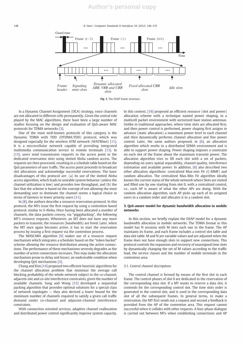
The downlink channel time is divided into time frames of equallength, which are, in turn, divided into a number of time slots [1,7].The channel frame duration accommodates 111 slots shared amongdynamic and fixed applications-based allocation. Fixed allocationrequires a certain guaranteed timeslots to be assigned while theconnection is established. However, dynamic allocation ensures twotypes of timeslots: guaranteed and non-guaranteed. Each time slotincludes a single 56 bytes wireless ATM packet as adopted by manyprevious works [1,8–10] while it improves efficiently the bandwidthutilization rate. A slot allocation table (SAT) is used to manage andupdate the time slot allocation. In our study, we divide the downlinkframe in two intervals:
(a). The control interval, which is placed at the beginning of eachframe, and
(b). The information (or data) interval whichmay include idle slots.
The control interval comprises two fields: the frame header andthe signaling field. The frame header is the first downlink control slotused by the AP for signaling the beginning of a frame transmission anddenoting the current frame structure. The signaling fields divided intoa number of time slots in the downlink, corresponding to an equalnumber of request slots in the uplink, plus a fewmore slots needed forreasons which are explained in Section 3.2. Each signaling slot isdivided into two mini-slots of equal duration.
Uplink request slots are used by terminals to access the channeland make a slot reservation, and are placed at the beginning of eachtime similarly to the signaling slots in the downlink. Request slots arealso used by mobile terminals to acquire the additional informationslots when their bit rate increases.
The information interval consists of fixed allocated slots anddynamic allocated slots according the supported service classes. Weconsider four types of traffic in our study: Constant Bit Rate (CBR),Variable Bit Rate (VBR), Available Bit Rate (ABR) and Unspecified BitRate (UBR). Specific traffic and QoS parameters have been defined tocharacterize each service class. Based on the previous concepts andreferences, Fig. 1 presents our DSAP frame structure proposal todynamically allocate slots for different service classes.
For Constant Bit Rate (CBR) traffic, slot allocation is performedonce during call establishment. A fixed allocation of slots is assignedaccording to user requests. When CBR slots are no longer available,arriving CBR calls are blocked. Variable Bit Rate (VBR) slots areassigned based on a statistical multiplexing algorithm. Unused CBRand VBR slots are shared with other traffic classes. Arriving VBR callsare also blockedwhen VBR slots are not available. Finally, for AvailableBit Rate/Unspecified Bit Rate (ABR/UBR) traffics, slot allocation isperformed on a burst-by-burst basis via dynamic reservation of ABR/UBR slots and unused CBR and VBR slots. Since slots are apportionedfor CBR, VBR, and ABR/UBR categories, the channel is not dominatedby the most demanding user. In order to minimize the waste ofbandwidth due to collisions, reservation slots are divided inmini-slots[11].
2.4. Related works: bandwidth allocation strategies
For efficient utilization of the radio spectrum, a frequency reusescheme that is consistent with the objectives of increasing capacityand minimizing interference is required. A variety of channelassignment strategies have been developed to achieve these objec-tives. Channel assignment strategies can be classified as either fixed ordynamic [12]. In a Fixed Channel Assignment (FCA) strategy, each cellis allocated a predetermined set of voice channels. If all the channelsin that cell are occupied, the call is blocked and the subscriber does notreceive service.
147R. Ouni / Computer Standards & Interfaces 34 (2012) 146–155
Author's personal copy
In a Dynamic Channel Assignment (DCA) strategy, voice channelsare not allocated to different cells permanently. Given the central roleplayed by the MAC algorithms, there have been a large number ofstudies focusing on the design and evaluation of QoS-aware MACprotocols for TDMA networks [3].
One of the most well-known protocols of this category is theDynamic TDMA with TDD (DTDMA/TDD) protocol, which wasdesigned especially for the wireless ATM network (WATMnet) [11].It is a microcellular network capable of providing integratedmultimedia communication service to remote terminals [13]. In[13], users send transmission requests to the access point in thededicated reservation slots using slotted Aloha random access. Therequests are then processed, resulting in a schedule table based on theQoS parameters of user traffic. The access point proceeds to broadcastslot allocations and acknowledge successful reservations. The basicdisadvantages of this protocol are: (a) its use of the slotted Alohaaccess algorithm, which leads to unstable system behavior (unless thechannel utilization is low) and provides low throughput, and (b) thefact that the scheme is based on the concept of not allowing the mostdemanding user to dominate the channel seems a logical choice interms of fairness to lower priority users [11].
In [8], the authors describe a resource reservation protocol. In thisprotocol, the MTs issue the first request by using a contention-basedprotocol, similar to S-Aloha. Once having been allocated a number ofchannels, the data packets convey, via “piggybacking”, the followingMT’s resource requests. Whenever, an MT does not have any morepackets to transmit, the resources (bandwidth) are freed. Later, whenthe MT once again becomes active, it has to start the reservationprocess by issuing a first request via the contention process.
The MASCARA algorithm [9] makes use of a resource requestmechanism which integrates a scheduler based on the "token bucket"scheme allowing the resource distribution among the active connec-tions. The performance of these mechanisms severely degrades as thenumber of active connections increases. This may make the allocationmechanism prone to delay and losses; an undesirable condition whendeveloping QoS mechanisms [3].
Chang and Kim [14] proposed two efficient heuristic algorithms forthe channel allocation problem that minimize the average callblocking probability of the whole network subject to the co-channel,adjacent-site and co-site interference constraints, given the number ofavailable channels. Sung and Wong [15] developed a sequentialpacking algorithm that provides optimal solutions for a special classof network topologies — they also derived a lower bound for theminimum number of channels required to satisfy a given call trafficdemand under co-channel and adjacent-channel interferenceconstraints.
With connection oriented services, adaptive channel reallocationand distributed power control significantly improve system capacity.
In this context, [16] proposed an efficient resource (slot and power)allocation scheme with a technique named power shaping, in amulticell packet environment with sectorized base station antennas.Unlike in traditional approaches, where time slots are allocated first,and then power control is performed, power shaping first assigns inadvance (static allocation) a maximum power level to each channeland then dynamically performs channel allocation and fine powercontrol. Later, the same authors proposed, in [6], an allocationalgorithm which works in a distributed SDMA environment and isable to support power shaping. Power shaping imposes a constrainton each slot of the frame about the maximum transmit power. Theallocation algorithm tries to fill each slot with a set of packets,depending on users spatial separability, channel quality, interferenceestimation and available power. In addition, [6] also described twoother allocation algorithms: centralized Max-min Fit (C-MMF) andrandom allocation. The centralized Max-Min Fit algorithm ideallyknows the current status of the whole network where Slots are visitedand filled one by one starting from slot 0, with a centralized control,i.e., each AP is aware of what the other APs are doing. With therandom allocation algorithm, each AP picks up each of its assignedusers in a random order and allocates it to a random slot.
3. QoS-aware model for dynamic bandwidth allocation in mobilenetworks
In this section, we briefly explain the DSAP model for a dynamicbandwidth allocation in mobile networks. The TDMA format in thismodel has N sessions with M slots each one in the frame. The APmaintains its frame, and each frame includes a control slot table anddata slot table. M and N are variable values and are adjusted when theframe does not have enough slots to support new connections. Thisprotocol controls the expansion and recovery of unassigned time slotsby dynamically changing the set of M values according to the trafficload, the service classes and the number of mobile terminals in thecontention area.
3.1. Control channel descriptions
The control channel is formed by means of the first slot in eachframe. The control phases of slot 0 are dedicated to the reservation ofthe corresponding data slot. If a MT wants to reserve a data slot, itcontends for the corresponding control slot. The time slots order isgenerated in the control slot, and is used in the corresponding dataslot of all the subsequent frames. In general terms, to make areservation, the MT first sends out a request and second a feedback isprovided from the AP of the contention area. This request cannotsuccessful when it collides with other requests. A four-phase dialogueis carried out between MTs when establishing connections and AP
Frame (i - 1) Frame ( i ) Frame (i+1)
Guard time
Time
… … …
Frame header
Signaling mini-slots
Dynamic allocated ABR, VBR and UBR
slots
Fixed allocated CBR slots Idle slots
… … …
Fig. 1. The DSAP frame structure.
148 R. Ouni / Computer Standards & Interfaces 34 (2012) 146–155
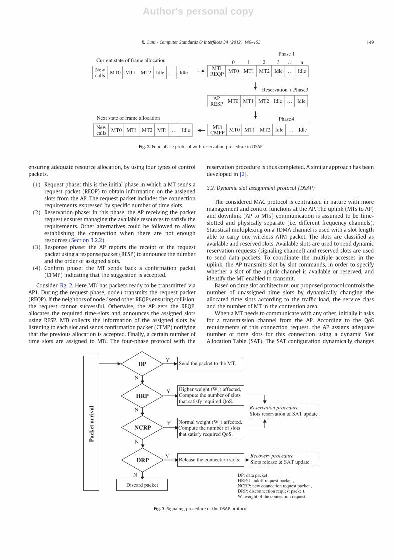
Author's personal copy
ensuring adequate resource allocation, by using four types of controlpackets.
(1). Request phase: this is the initial phase in which a MT sends arequest packet (REQP) to obtain information on the assignedslots from the AP. The request packet includes the connectionrequirements expressed by specific number of time slots.
(2). Reservation phase: In this phase, the AP receiving the packetrequest ensures managing the available resources to satisfy therequirements. Other alternatives could be followed to allowestablishing the connection when there are not enoughresources (Section 3.2.2).
(3). Response phase: the AP reports the receipt of the requestpacket using a response packet (RESP) to announce the numberand the order of assigned slots.
(4). Confirm phase: the MT sends back a confirmation packet(CFMP) indicating that the suggestion is accepted.
Consider Fig. 2. Here MTi has packets ready to be transmitted viaAP1. During the request phase, node i transmits the request packet(REQP). If the neighbors of node i send other REQPs ensuring collision,the request cannot successful. Otherwise, the AP gets the REQP,allocates the required time-slots and announces the assigned slotsusing RESP. MTi collects the information of the assigned slots bylistening to each slot and sends confirmation packet (CFMP) notifyingthat the previous allocation is accepted. Finally, a certain number oftime slots are assigned to MTi. The four-phase protocol with the
reservation procedure is thus completed. A similar approach has beendeveloped in [2].
3.2. Dynamic slot assignment protocol (DSAP)
The considered MAC protocol is centralized in nature with moremanagement and control functions at the AP. The uplink (MTs to AP)and downlink (AP to MTs) communication is assumed to be time-slotted and physically separate (i.e. different frequency channels).Statistical multiplexing on a TDMA channel is used with a slot lengthable to carry one wireless ATM packet. The slots are classified asavailable and reserved slots. Available slots are used to send dynamicreservation requests (signaling channel) and reserved slots are usedto send data packets. To coordinate the multiple accesses in theuplink, the AP transmits slot-by-slot commands, in order to specifywhether a slot of the uplink channel is available or reserved, andidentify the MT enabled to transmit.
Based on time slot architecture, our proposed protocol controls thenumber of unassigned time slots by dynamically changing theallocated time slots according to the traffic load, the service classand the number of MT in the contention area.
When a MT needs to communicate with any other, initially it asksfor a transmission channel from the AP. According to the QoSrequirements of this connection request, the AP assigns adequatenumber of time slots for this connection using a dynamic SlotAllocation Table (SAT). The SAT configuration dynamically changes
Pac
ket
arri
val
DP
HRP
DRP
Y
Y
Y
N
N
N
Send the packet to the MT.
Higher weight (Wh) affected, Compute the number of slotsthat satisfy required QoS.
Release the connection slots.
NCRPY
N
Normal weight (Wn) affected,Compute the number of slotsthat satisfy required QoS.
Discard packet
DP: data packet ,HRP: handoff request packet ,NCRP: new connection request packet ,DRP: disconnection request packe t,W: weight of the connection request.
Reservation procedureSlots reservation & SAT update
Recovery procedureSlots release & SAT update
Fig. 3. Signaling procedure of the DSAP protocol.
New calls MT0 MT1 MT2 Idle … Idle
0 1 2 3 … nMTi
REQP MT0 MT1 MT2 Idle … Idle
AP RESP MT0 MT1 MT2 Idle … Idle
MTi CMFP MT0 MT1 MT2 Idle … IdleNew
calls MT0 MT1 MT2 MTi … Idle
Current state of frame allocation
Next state of frame allocation
Phase 1
Reservation + Phase3
Phase4
Fig. 2. Four-phase protocol with reservation procedure in DSAP.
149R. Ouni / Computer Standards & Interfaces 34 (2012) 146–155
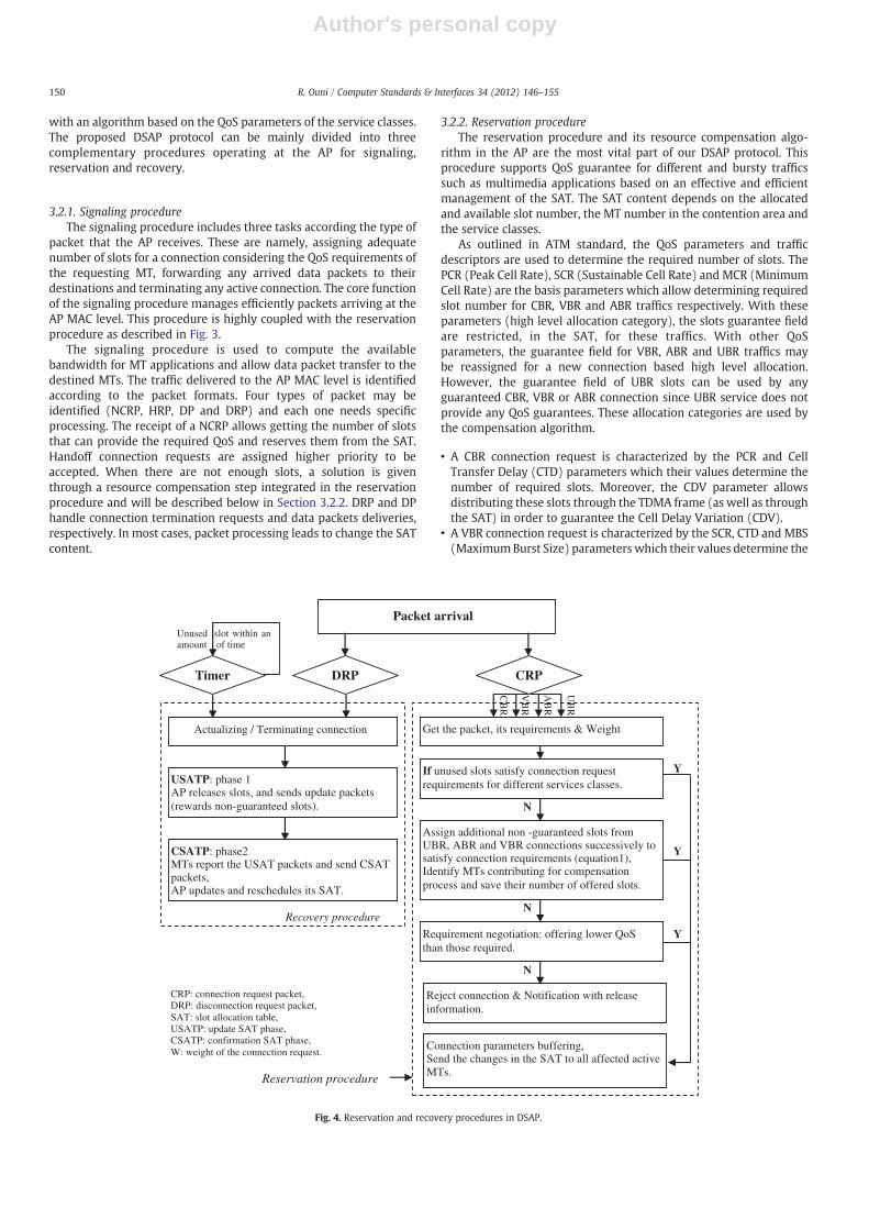
Author's personal copy
with an algorithm based on the QoS parameters of the service classes.The proposed DSAP protocol can be mainly divided into threecomplementary procedures operating at the AP for signaling,reservation and recovery.
3.2.1. Signaling procedureThe signaling procedure includes three tasks according the type of
packet that the AP receives. These are namely, assigning adequatenumber of slots for a connection considering the QoS requirements ofthe requesting MT, forwarding any arrived data packets to theirdestinations and terminating any active connection. The core functionof the signaling procedure manages efficiently packets arriving at theAP MAC level. This procedure is highly coupled with the reservationprocedure as described in Fig. 3.
The signaling procedure is used to compute the availablebandwidth for MT applications and allow data packet transfer to thedestined MTs. The traffic delivered to the AP MAC level is identifiedaccording to the packet formats. Four types of packet may beidentified (NCRP, HRP, DP and DRP) and each one needs specificprocessing. The receipt of a NCRP allows getting the number of slotsthat can provide the required QoS and reserves them from the SAT.Handoff connection requests are assigned higher priority to beaccepted. When there are not enough slots, a solution is giventhrough a resource compensation step integrated in the reservationprocedure and will be described below in Section 3.2.2. DRP and DPhandle connection termination requests and data packets deliveries,respectively. In most cases, packet processing leads to change the SATcontent.
3.2.2. Reservation procedureThe reservation procedure and its resource compensation algo-
rithm in the AP are the most vital part of our DSAP protocol. Thisprocedure supports QoS guarantee for different and bursty trafficssuch as multimedia applications based on an effective and efficientmanagement of the SAT. The SAT content depends on the allocatedand available slot number, the MT number in the contention area andthe service classes.
As outlined in ATM standard, the QoS parameters and trafficdescriptors are used to determine the required number of slots. ThePCR (Peak Cell Rate), SCR (Sustainable Cell Rate) and MCR (MinimumCell Rate) are the basis parameters which allow determining requiredslot number for CBR, VBR and ABR traffics respectively. With theseparameters (high level allocation category), the slots guarantee fieldare restricted, in the SAT, for these traffics. With other QoSparameters, the guarantee field for VBR, ABR and UBR traffics maybe reassigned for a new connection based high level allocation.However, the guarantee field of UBR slots can be used by anyguaranteed CBR, VBR or ABR connection since UBR service does notprovide any QoS guarantees. These allocation categories are used bythe compensation algorithm.
• A CBR connection request is characterized by the PCR and CellTransfer Delay (CTD) parameters which their values determine thenumber of required slots. Moreover, the CDV parameter allowsdistributing these slots through the TDMA frame (as well as throughthe SAT) in order to guarantee the Cell Delay Variation (CDV).
• A VBR connection request is characterized by the SCR, CTD and MBS(MaximumBurst Size) parameters which their values determine the
Y
Y
Y
N
N
N
Packet arrival
CB
R
VB
R
AB
R
UB
R
If unused slots satisfy connection request requirements for different services classes.
Actualizing / Terminating connection
DRPTimer
Assign additional non -guaranteed slots from UBR, ABR and VBR connections successively to satisfy connection requirements (equation1),Identify MTs contributing for compensation process and save their number of offered slots.
Get the packet, its requirements & Weight
Requirement negotiation: offering lower QoS than those required.
Reject connection & Notification with release information.
Connection parameters buffering,Send the changes in the SAT to all affected active MTs.
USATP: phase 1AP releases slots, and sends update packets (rewards non-guaranteed slots).
CSATP: phase2MTs report the USAT packets and send CSAT packets,AP updates and reschedules its SAT.
Recovery procedure
Reservation procedure
CRP
Unused slot within anamount of time
CRP: connection request packet, DRP: disconnection request packet,SAT: slot allocation table,USATP: update SAT phase,CSATP: confirmation SAT phase,W: weight of the connection request.
Fig. 4. Reservation and recovery procedures in DSAP.
150 R. Ouni / Computer Standards & Interfaces 34 (2012) 146–155
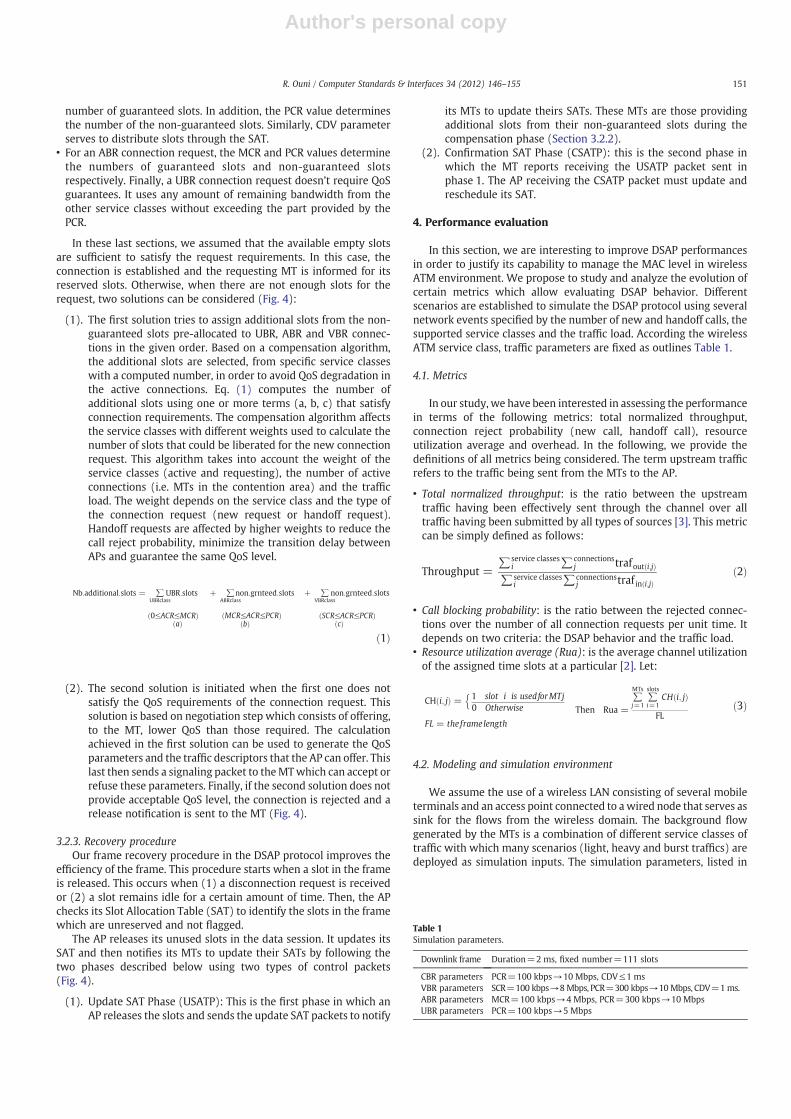
Author's personal copy
number of guaranteed slots. In addition, the PCR value determinesthe number of the non-guaranteed slots. Similarly, CDV parameterserves to distribute slots through the SAT.
• For an ABR connection request, the MCR and PCR values determinethe numbers of guaranteed slots and non-guaranteed slotsrespectively. Finally, a UBR connection request doesn’t require QoSguarantees. It uses any amount of remaining bandwidth from theother service classes without exceeding the part provided by thePCR.
In these last sections, we assumed that the available empty slotsare sufficient to satisfy the request requirements. In this case, theconnection is established and the requesting MT is informed for itsreserved slots. Otherwise, when there are not enough slots for therequest, two solutions can be considered (Fig. 4):
(1). The first solution tries to assign additional slots from the non-guaranteed slots pre-allocated to UBR, ABR and VBR connec-tions in the given order. Based on a compensation algorithm,the additional slots are selected, from specific service classeswith a computed number, in order to avoid QoS degradation inthe active connections. Eq. (1) computes the number ofadditional slots using one or more terms (a, b, c) that satisfyconnection requirements. The compensation algorithm affectsthe service classes with different weights used to calculate thenumber of slots that could be liberated for the new connectionrequest. This algorithm takes into account the weight of theservice classes (active and requesting), the number of activeconnections (i.e. MTs in the contention area) and the trafficload. The weight depends on the service class and the type ofthe connection request (new request or handoff request).Handoff requests are affected by higher weights to reduce thecall reject probability, minimize the transition delay betweenAPs and guarantee the same QoS level.
Nb:additional:slots = ∑UBRclass
UBR:slots + ∑ABRclass
non:grnteed:slots + ∑VBRclass
non:grnteed:slots
0≤ACR≤MCRð Það Þ
MCR≤ACR≤PCRð Þbð Þ
SCR≤ACR≤PCRð Þcð Þ
ð1Þ
(2). The second solution is initiated when the first one does notsatisfy the QoS requirements of the connection request. Thissolution is based on negotiation step which consists of offering,to the MT, lower QoS than those required. The calculationachieved in the first solution can be used to generate the QoSparameters and the traffic descriptors that the AP can offer. Thislast then sends a signaling packet to theMTwhich can accept orrefuse these parameters. Finally, if the second solution does notprovide acceptable QoS level, the connection is rejected and arelease notification is sent to the MT (Fig. 4).
3.2.3. Recovery procedureOur frame recovery procedure in the DSAP protocol improves the
efficiency of the frame. This procedure starts when a slot in the frameis released. This occurs when (1) a disconnection request is receivedor (2) a slot remains idle for a certain amount of time. Then, the APchecks its Slot Allocation Table (SAT) to identify the slots in the framewhich are unreserved and not flagged.
The AP releases its unused slots in the data session. It updates itsSAT and then notifies its MTs to update their SATs by following thetwo phases described below using two types of control packets(Fig. 4).
(1). Update SAT Phase (USATP): This is the first phase in which anAP releases the slots and sends the update SAT packets to notify
its MTs to update theirs SATs. These MTs are those providingadditional slots from their non-guaranteed slots during thecompensation phase (Section 3.2.2).
(2). Confirmation SAT Phase (CSATP): this is the second phase inwhich the MT reports receiving the USATP packet sent inphase 1. The AP receiving the CSATP packet must update andreschedule its SAT.
4. Performance evaluation
In this section, we are interesting to improve DSAP performancesin order to justify its capability to manage the MAC level in wirelessATM environment. We propose to study and analyze the evolution ofcertain metrics which allow evaluating DSAP behavior. Differentscenarios are established to simulate the DSAP protocol using severalnetwork events specified by the number of new and handoff calls, thesupported service classes and the traffic load. According the wirelessATM service class, traffic parameters are fixed as outlines Table 1.
4.1. Metrics
In our study, we have been interested in assessing the performancein terms of the following metrics: total normalized throughput,connection reject probability (new call, handoff call), resourceutilization average and overhead. In the following, we provide thedefinitions of all metrics being considered. The term upstream trafficrefers to the traffic being sent from the MTs to the AP.
• Total normalized throughput: is the ratio between the upstreamtraffic having been effectively sent through the channel over alltraffic having been submitted by all types of sources [3]. This metriccan be simply defined as follows:
Throughput =∑service classes
i ∑connectionsj trafout i;jð Þ
∑service classesi ∑connections
j traf in i;jð Þð2Þ
• Call blocking probability: is the ratio between the rejected connec-tions over the number of all connection requests per unit time. Itdepends on two criteria: the DSAP behavior and the traffic load.
• Resource utilization average (Rua): is the average channel utilizationof the assigned time slots at a particular [2]. Let:
CH i; jð Þ =n1 slot i is usedforMTj0 Otherwise
FL = the framelength
Then Rua =∑MTs
j=1∑slots
i=1CH i; jð Þ
FLð3Þ
4.2. Modeling and simulation environment
We assume the use of a wireless LAN consisting of several mobileterminals and an access point connected to awired node that serves assink for the flows from the wireless domain. The background flowgenerated by the MTs is a combination of different service classes oftraffic with which many scenarios (light, heavy and burst traffics) aredeployed as simulation inputs. The simulation parameters, listed in
Table 1Simulation parameters.
Downlink frame Duration=2 ms, fixed number=111 slots
CBR parameters PCR=100 kbps→10 Mbps, CDV≤1 msVBR parameters SCR=100 kbps→8Mbps, PCR=300 kbps→10Mbps, CDV=1ms.ABR parameters MCR=100 kbps→4 Mbps, PCR=300 kbps→10 MbpsUBR parameters PCR=100 kbps→5 Mbps
151R. Ouni / Computer Standards & Interfaces 34 (2012) 146–155
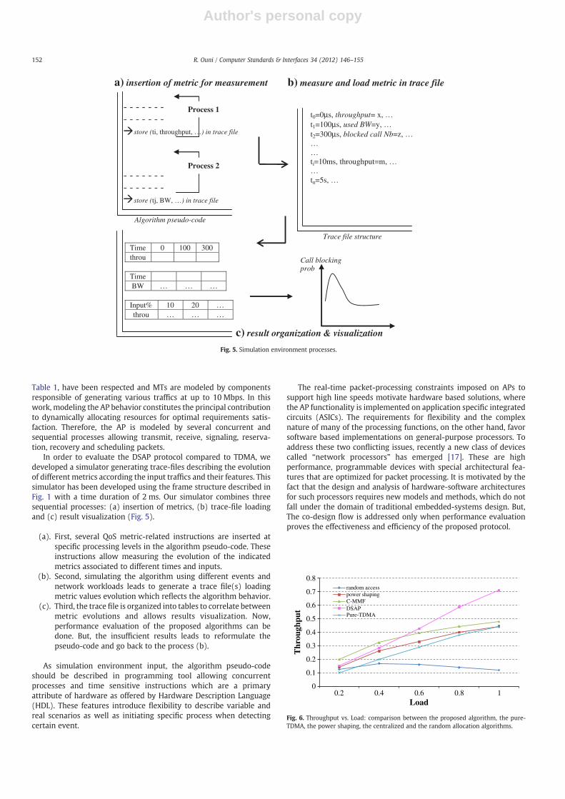
Author's personal copy
Table 1, have been respected and MTs are modeled by componentsresponsible of generating various traffics at up to 10 Mbps. In thiswork, modeling the AP behavior constitutes the principal contributionto dynamically allocating resources for optimal requirements satis-faction. Therefore, the AP is modeled by several concurrent andsequential processes allowing transmit, receive, signaling, reserva-tion, recovery and scheduling packets.
In order to evaluate the DSAP protocol compared to TDMA, wedeveloped a simulator generating trace-files describing the evolutionof different metrics according the input traffics and their features. Thissimulator has been developed using the frame structure described inFig. 1 with a time duration of 2 ms. Our simulator combines threesequential processes: (a) insertion of metrics, (b) trace-file loadingand (c) result visualization (Fig. 5).
(a). First, several QoS metric-related instructions are inserted atspecific processing levels in the algorithm pseudo-code. Theseinstructions allow measuring the evolution of the indicatedmetrics associated to different times and inputs.
(b). Second, simulating the algorithm using different events andnetwork workloads leads to generate a trace file(s) loadingmetric values evolution which reflects the algorithm behavior.
(c). Third, the trace file is organized into tables to correlate betweenmetric evolutions and allows results visualization. Now,performance evaluation of the proposed algorithms can bedone. But, the insufficient results leads to reformulate thepseudo-code and go back to the process (b).
As simulation environment input, the algorithm pseudo-codeshould be described in programming tool allowing concurrentprocesses and time sensitive instructions which are a primaryattribute of hardware as offered by Hardware Description Language(HDL). These features introduce flexibility to describe variable andreal scenarios as well as initiating specific process when detectingcertain event.
The real-time packet-processing constraints imposed on APs tosupport high line speeds motivate hardware based solutions, wherethe AP functionality is implemented on application specific integratedcircuits (ASICs). The requirements for flexibility and the complexnature of many of the processing functions, on the other hand, favorsoftware based implementations on general-purpose processors. Toaddress these two conflicting issues, recently a new class of devicescalled “network processors” has emerged [17]. These are highperformance, programmable devices with special architectural fea-tures that are optimized for packet processing. It is motivated by thefact that the design and analysis of hardware-software architecturesfor such processors requires new models and methods, which do notfall under the domain of traditional embedded-systems design. But,The co-design flow is addressed only when performance evaluationproves the effectiveness and efficiency of the proposed protocol.
- - - - - - -- - - - - - -
store (ti, throughput, …) in trace file
- - - - - - -- - - - - - -
store (tj, BW, …) in trace file
Process 1
Process 2
a) insertion of metric for measurement
t0=0µs, throughput= x, …t1=100µs, used BW=y, …t2=300µs, blocked call Nb=z, ………ti=10ms, throughput=m, ……tn=5s, …
b) measure and load metric in trace file
Algorithm pseudo-code
Trace file structure
Time 0 100 300throu
TimeBW … … …
Input% 10 20 …throu … … …
c) result organization & visualization
Call blocking prob
Fig. 5. Simulation environment processes.
0
0.1
0.2
0.3
0.4
0.5
0.6
0.7
0.8
0.2 0.4 0.6 0.8 1
random accesspower shapingC-MMFDSAPPure-TDMA
Thr
ough
put
Load
Fig. 6. Throughput vs. Load: comparison between the proposed algorithm, the pure-TDMA, the power shaping, the centralized and the random allocation algorithms.
152 R. Ouni / Computer Standards & Interfaces 34 (2012) 146–155
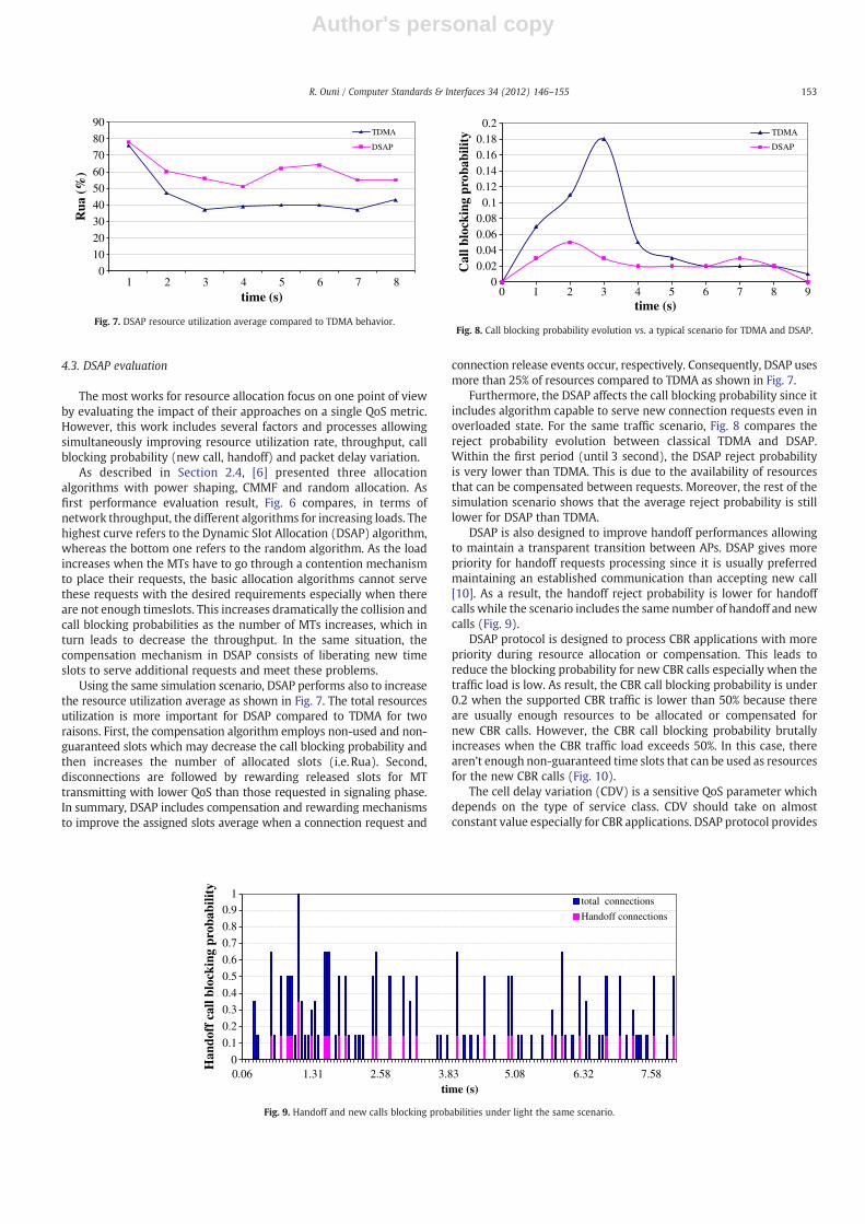
Author's personal copy
4.3. DSAP evaluation
The most works for resource allocation focus on one point of viewby evaluating the impact of their approaches on a single QoS metric.However, this work includes several factors and processes allowingsimultaneously improving resource utilization rate, throughput, callblocking probability (new call, handoff) and packet delay variation.
As described in Section 2.4, [6] presented three allocationalgorithms with power shaping, CMMF and random allocation. Asfirst performance evaluation result, Fig. 6 compares, in terms ofnetwork throughput, the different algorithms for increasing loads. Thehighest curve refers to the Dynamic Slot Allocation (DSAP) algorithm,whereas the bottom one refers to the random algorithm. As the loadincreases when the MTs have to go through a contention mechanismto place their requests, the basic allocation algorithms cannot servethese requests with the desired requirements especially when thereare not enough timeslots. This increases dramatically the collision andcall blocking probabilities as the number of MTs increases, which inturn leads to decrease the throughput. In the same situation, thecompensation mechanism in DSAP consists of liberating new timeslots to serve additional requests and meet these problems.
Using the same simulation scenario, DSAP performs also to increasethe resource utilization average as shown in Fig. 7. The total resourcesutilization is more important for DSAP compared to TDMA for tworaisons. First, the compensation algorithm employs non-used and non-guaranteed slots which may decrease the call blocking probability andthen increases the number of allocated slots (i.e.Rua). Second,disconnections are followed by rewarding released slots for MTtransmitting with lower QoS than those requested in signaling phase.In summary, DSAP includes compensation and rewarding mechanismsto improve the assigned slots average when a connection request and
connection release events occur, respectively. Consequently, DSAP usesmore than 25% of resources compared to TDMA as shown in Fig. 7.
Furthermore, the DSAP affects the call blocking probability since itincludes algorithm capable to serve new connection requests even inoverloaded state. For the same traffic scenario, Fig. 8 compares thereject probability evolution between classical TDMA and DSAP.Within the first period (until 3 second), the DSAP reject probabilityis very lower than TDMA. This is due to the availability of resourcesthat can be compensated between requests. Moreover, the rest of thesimulation scenario shows that the average reject probability is stilllower for DSAP than TDMA.
DSAP is also designed to improve handoff performances allowingto maintain a transparent transition between APs. DSAP gives morepriority for handoff requests processing since it is usually preferredmaintaining an established communication than accepting new call[10]. As a result, the handoff reject probability is lower for handoffcalls while the scenario includes the same number of handoff and newcalls (Fig. 9).
DSAP protocol is designed to process CBR applications with morepriority during resource allocation or compensation. This leads toreduce the blocking probability for new CBR calls especially when thetraffic load is low. As result, the CBR call blocking probability is under0.2 when the supported CBR traffic is lower than 50% because thereare usually enough resources to be allocated or compensated fornew CBR calls. However, the CBR call blocking probability brutallyincreases when the CBR traffic load exceeds 50%. In this case, therearen’t enough non-guaranteed time slots that can be used as resourcesfor the new CBR calls (Fig. 10).
The cell delay variation (CDV) is a sensitive QoS parameter whichdepends on the type of service class. CDV should take on almostconstant value especially for CBR applications. DSAP protocol provides
0
10
20
30
40
50
60
70
80
90
1 2 3 4 5 6 7 8
Rua
(%)
time (s)
TDMA
DSAP
Fig. 7. DSAP resource utilization average compared to TDMA behavior.
00.020.040.060.08
0.10.120.140.160.18
0.2
0 1 2 3 4 5 6 7 8 9
Cal
l blo
ckin
g pr
obab
ility
time (s)
TDMA
DSAP
Fig. 8. Call blocking probability evolution vs. a typical scenario for TDMA and DSAP.
0
0.1
0.06 1.31 2.58 3.83 5.08 6.32 7.58
0.2
0.3
0.4
0.5
0.6
0.7
0.8
0.91
Han
doff
cal
l blo
ckin
g pr
obab
ility
time (s)
total connections
Handoff connections
Fig. 9. Handoff and new calls blocking probabilities under light the same scenario.
153R. Ouni / Computer Standards & Interfaces 34 (2012) 146–155
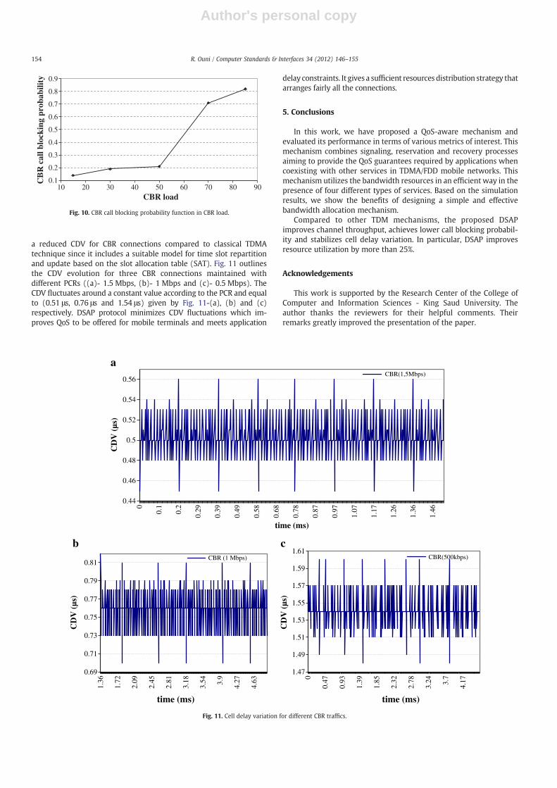
Author's personal copy
a reduced CDV for CBR connections compared to classical TDMAtechnique since it includes a suitable model for time slot repartitionand update based on the slot allocation table (SAT). Fig. 11 outlinesthe CDV evolution for three CBR connections maintained withdifferent PCRs ((a)- 1.5 Mbps, (b)- 1 Mbps and (c)- 0.5 Mbps). TheCDV fluctuates around a constant value according to the PCR and equalto (0.51 μs, 0.76 μs and 1.54 μs) given by Fig. 11-(a), (b) and (c)respectively. DSAP protocol minimizes CDV fluctuations which im-proves QoS to be offered for mobile terminals and meets application
delay constraints. It gives a sufficient resources distribution strategy thatarranges fairly all the connections.
5. Conclusions
In this work, we have proposed a QoS-aware mechanism andevaluated its performance in terms of various metrics of interest. Thismechanism combines signaling, reservation and recovery processesaiming to provide the QoS guarantees required by applications whencoexisting with other services in TDMA/FDD mobile networks. Thismechanism utilizes the bandwidth resources in an efficient way in thepresence of four different types of services. Based on the simulationresults, we show the benefits of designing a simple and effectivebandwidth allocation mechanism.
Compared to other TDM mechanisms, the proposed DSAPimproves channel throughput, achieves lower call blocking probabil-ity and stabilizes cell delay variation. In particular, DSAP improvesresource utilization by more than 25%.
Acknowledgements
This work is supported by the Research Center of the College ofComputer and Information Sciences - King Saud University. Theauthor thanks the reviewers for their helpful comments. Theirremarks greatly improved the presentation of the paper.
0.1
0.2
0.3
0.4
0.5
0.6
0.7
0.8
0.9
10 20 30 40 50 60 70 80 90
CB
R c
all b
lock
ing
prob
abili
ty
CBR load
Fig. 10. CBR call blocking probability function in CBR load.
0.44
0.46
0.48
0.5
0.52
0.54
0.56
0
0.1
0.2
0.29
0.39
0.49
0.58
0.68
0.78
0.87
0.97
1.07
1.17
1.26
1.36
1.46
CD
V (
µs)
time (ms)
CBR(1,5Mbps)
0.69
0.71
0.73
0.75
0.77
0.79
0.81
1.36
1.72
2.09
2.45
2.81
3.18
3.54 3.9
4.27
4.63
CD
V (
µs)
time (ms)
CBR (1 Mbps)
1.47
1.49
1.51
1.53
1.55
1.57
1.59
1.61
0
0.47
0.93
1.39
1.85
2.32
2.78
3.24 3.7
4.17
CD
V (
µs)
time (ms)
CBR(500kbps)
a
b c
Fig. 11. Cell delay variation for different CBR traffics.
154 R. Ouni / Computer Standards & Interfaces 34 (2012) 146–155
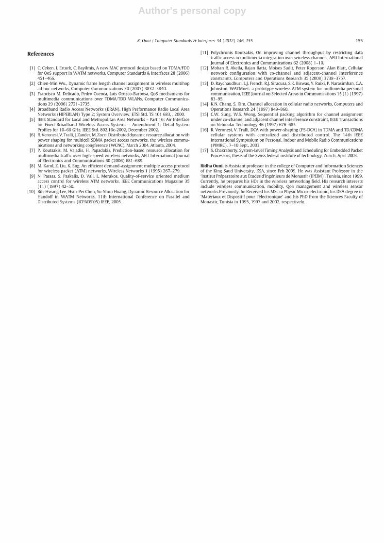
Author's personal copy
References
[1] C. Ceken, I. Erturk, C. Bayilmis, A new MAC protocol design based on TDMA/FDDfor QoS support in WATM networks, Computer Standards & Interfaces 28 (2006)451–466.
[2] Chien-Min Wu., Dynamic frame length channel assignment in wireless multihopad hoc networks, Computer Communications 30 (2007) 3832–3840.
[3] Francisco M. Delicado, Pedro Cuenca, Luis Orozco-Barbosa, QoS mechanisms formultimedia communications over TDMA/TDD WLANs, Computer Communica-tions 29 (2006) 2721–2735.
[4] Broadband Radio Access Networks (BRAN), High Performance Radio Local AreaNetworks (HIPERLAN) Type 2; System Overview, ETSI Std. TS 101 683, , 2000.
[5] IEEE Standard for Local and Metropolitan Area Networks – Part 16: Air Interfacefor Fixed Broadband Wireless Access Systems – Amendment 1: Detail SystemProfiles for 10–66 GHz, IEEE Std. 802.16c-2002, December 2002.
[6] R.Veronesi, V. Tralli, J. Zander,M. Zorzi, Distributeddynamic resource allocationwithpower shaping for multicell SDMA packet access networks, the wireless commu-nications and networking congference (WCNC), March 2004, Atlanta, 2004.
[7] P. Koutsakis, M. Va.adis, H. Papadakis, Prediction-based resource allocation formultimedia traffic over high-speed wireless networks, AEU International Journalof Electronics and Communications 60 (2006) 681–689.
[8] M. Karol, Z. Liu, K. Eng, An efficient demand-assignment multiple access protocolfor wireless packet (ATM) networks, Wireless Networks 1 (1995) 267–279.
[9] N. Passas, S. Paskalis, D. Vali, L. Merakos, Quality-of-service oriented mediumaccess control for wireless ATM networks, IEEE Communications Magazine 35(11) (1997) 42–50.
[10] Bih-Hwang Lee, Hsin-Pei Chen, Su-Shun Huang, Dynamic Resource Allocation forHandoff in WATM Networks, 11th International Conference on Parallel andDistributed Systems (ICPADS’05) IEEE, 2005.
[11] Polychronis Koutsakis, On improving channel throughput by restricting datatraffic access in multimedia integration over wireless channels, AEU InternationalJournal of Electronics and Communications 62 (2008) 1–10.
[12] Mohan R. Akella, Rajan Batta, Moises Sudit, Peter Rogerson, Alan Blatt, Cellularnetwork configuration with co-channel and adjacent-channel interferenceconstraints, Computers and Operations Research 35 (2008) 3738–3757.
[13] D. Raychaudhuri, L.J. French, R.J. Siracusa, S.K. Biswas, Y. Ruixi, P. Narasimhan, C.A.Johnston, WATMnet: a prototype wireless ATM system for multimedia personalcommunication, IEEE Journal on Selected Areas in Communications 15 (1) (1997)83–95.
[14] K.N. Chang, S. Kim, Channel allocation in cellular radio networks, Computers andOperations Research 24 (1997) 849–860.
[15] C.W. Sung, W.S. Wong, Sequential packing algorithm for channel assignmentunder co-channel and adjacent channel interference constraint, IEEE Transactionson Vehicular Technology 46 (1997) 676–685.
[16] R. Veronesi, V. Tralli, DCA with power-shaping (PS-DCA) in TDMA and TD/CDMAcellular systems with centralized and distributed control, The 14th IEEEInternational Symposium on Personal, Indoor and Mobile Radio Communications(PIMRC), 7–10 Sept, 2003.
[17] S. Chakraborty, System-Level Timing Analysis and Scheduling for Embedded PacketProcessors, thesis of the Swiss federal institute of technology, Zurich, April 2003.
Ridha Ouni. is Assistant professor in the college of Computer and Information Sciencesof the King Saud University, KSA, since Feb 2009. He was Assistant Professor in the‘Institut Préparatoire aux Études d'Ingénieurs de Monastir (IPEIM)’, Tunisia, since 1999.Currently, he prepares his HDr in the wireless networking field. His research interestsinclude wireless communication, mobility, QoS management and wireless sensornetworks.Previously, he Received his MSc in Physic Micro-electronic, his DEA degree in‘Matériaux et Dispositif pour l'électronique’ and his PhD from the Sciences Faculty ofMonastir, Tunisia in 1995, 1997 and 2002, respectively.
155R. Ouni / Computer Standards & Interfaces 34 (2012) 146–155
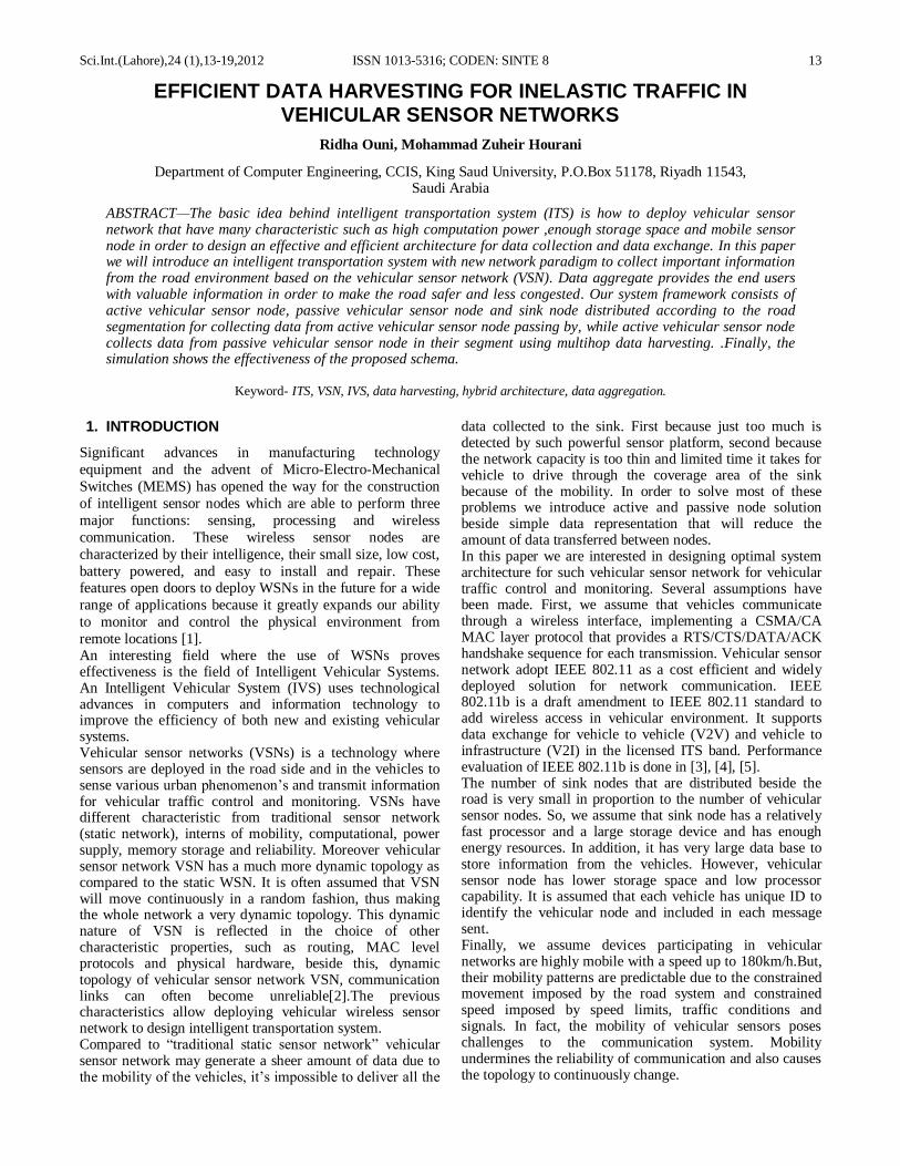
Sci.Int.(Lahore),24 (1),13-19,2012 ISSN 1013-5316; CODEN: SINTE 8
13
EFFICIENT DATA HARVESTING FOR INELASTIC TRAFFIC IN VEHICULAR SENSOR NETWORKS
Ridha Ouni, Mohammad Zuheir Hourani
Department of Computer Engineering, CCIS, King Saud University, P.O.Box 51178, Riyadh 11543, Saudi Arabia
ABSTRACT—The basic idea behind intelligent transportation system (ITS) is how to deploy vehicular sensor network that have many characteristic such as high computation power ,enough storage space and mobile sensor node in order to design an effective and efficient architecture for data collection and data exchange. In this paper we will introduce an intelligent transportation system with new network paradigm to collect important information from the road environment based on the vehicular sensor network (VSN). Data aggregate provides the end users with valuable information in order to make the road safer and less congested. Our system framework consists of active vehicular sensor node, passive vehicular sensor node and sink node distributed according to the road segmentation for collecting data from active vehicular sensor node passing by, while active vehicular sensor node collects data from passive vehicular sensor node in their segment using multihop data harvesting. .Finally, the simulation shows the effectiveness of the proposed schema.
Keyword- ITS, VSN, IVS, data harvesting, hybrid architecture, data aggregation.
1. INTRODUCTION
Significant advances in manufacturing technology
equipment and the advent of Micro-Electro-Mechanical
Switches (MEMS) has opened the way for the construction
of intelligent sensor nodes which are able to perform three
major functions: sensing, processing and wireless
communication. These wireless sensor nodes are
characterized by their intelligence, their small size, low cost,
battery powered, and easy to install and repair. These features open doors to deploy WSNs in the future for a wide
range of applications because it greatly expands our ability
to monitor and control the physical environment from
remote locations [1]. An interesting field where the use of WSNs proves effectiveness is the field of Intelligent Vehicular Systems. An Intelligent Vehicular System (IVS) uses technological advances in computers and information technology to improve the efficiency of both new and existing vehicular systems. Vehicular sensor networks (VSNs) is a technology where sensors are deployed in the road side and in the vehicles to sense various urban phenomenon’s and transmit information for vehicular traffic control and monitoring. VSNs have different characteristic from traditional sensor network (static network), interns of mobility, computational, power supply, memory storage and reliability. Moreover vehicular sensor network VSN has a much more dynamic topology as compared to the static WSN. It is often assumed that VSN will move continuously in a random fashion, thus making the whole network a very dynamic topology. This dynamic nature of VSN is reflected in the choice of other characteristic properties, such as routing, MAC level protocols and physical hardware, beside this, dynamic topology of vehicular sensor network VSN, communication links can often become unreliable[2].The previous characteristics allow deploying vehicular wireless sensor network to design intelligent transportation system. Compared to “traditional static sensor network” vehicular sensor network may generate a sheer amount of data due to the mobility of the vehicles, it’s impossible to deliver all the
data collected to the sink. First because just too much is detected by such powerful sensor platform, second because the network capacity is too thin and limited time it takes for vehicle to drive through the coverage area of the sink because of the mobility. In order to solve most of these problems we introduce active and passive node solution beside simple data representation that will reduce the amount of data transferred between nodes. In this paper we are interested in designing optimal system architecture for such vehicular sensor network for vehicular traffic control and monitoring. Several assumptions have been made. First, we assume that vehicles communicate through a wireless interface, implementing a CSMA/CA MAC layer protocol that provides a RTS/CTS/DATA/ACK handshake sequence for each transmission. Vehicular sensor network adopt IEEE 802.11 as a cost efficient and widely deployed solution for network communication. IEEE 802.11b is a draft amendment to IEEE 802.11 standard to add wireless access in vehicular environment. It supports data exchange for vehicle to vehicle (V2V) and vehicle to infrastructure (V2I) in the licensed ITS band. Performance evaluation of IEEE 802.11b is done in [3], [4], [5]. The number of sink nodes that are distributed beside the road is very small in proportion to the number of vehicular sensor nodes. So, we assume that sink node has a relatively fast processor and a large storage device and has enough energy resources. In addition, it has very large data base to store information from the vehicles. However, vehicular sensor node has lower storage space and low processor capability. It is assumed that each vehicle has unique ID to identify the vehicular node and included in each message sent. Finally, we assume devices participating in vehicular networks are highly mobile with a speed up to 180km/h.But, their mobility patterns are predictable due to the constrained movement imposed by the road system and constrained speed imposed by speed limits, traffic conditions and signals. In fact, the mobility of vehicular sensors poses challenges to the communication system. Mobility undermines the reliability of communication and also causes the topology to continuously change.
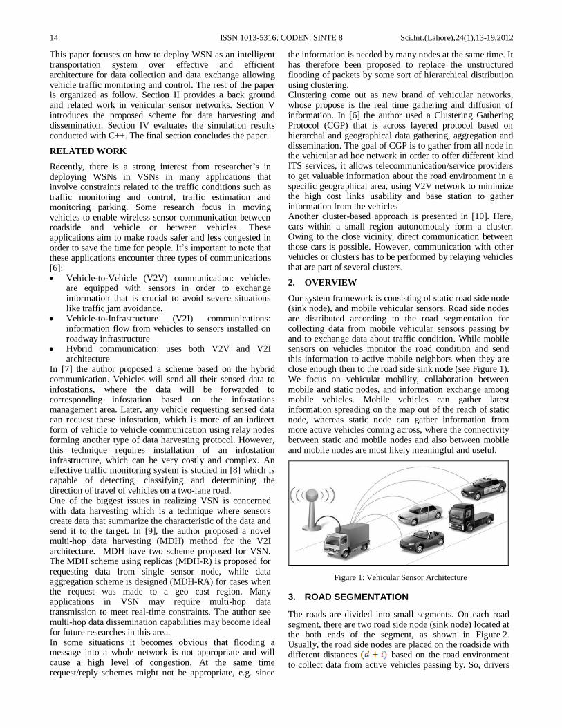
ISSN 1013-5316; CODEN: SINTE 8 Sci.Int.(Lahore),24(1),13-19,2012
14
This paper focuses on how to deploy WSN as an intelligent transportation system over effective and efficient architecture for data collection and data exchange allowing vehicle traffic monitoring and control. The rest of the paper is organized as follow. Section II provides a back ground and related work in vehicular sensor networks. Section V introduces the proposed scheme for data harvesting and dissemination. Section IV evaluates the simulation results conducted with C++. The final section concludes the paper.
RELATED WORK
Recently, there is a strong interest from researcher’s in deploying WSNs in VSNs in many applications that involve constraints related to the traffic conditions such as traffic monitoring and control, traffic estimation and monitoring parking. Some research focus in moving vehicles to enable wireless sensor communication between roadside and vehicle or between vehicles. These applications aim to make roads safer and less congested in order to save the time for people. It’s important to note that these applications encounter three types of communications [6]: Vehicle-to-Vehicle (V2V) communication: vehicles
are equipped with sensors in order to exchange information that is crucial to avoid severe situations like traffic jam avoidance.
Vehicle-to-Infrastructure (V2I) communications: information flow from vehicles to sensors installed on roadway infrastructure
Hybrid communication: uses both V2V and V2I architecture
In [7] the author proposed a scheme based on the hybrid communication. Vehicles will send all their sensed data to infostations, where the data will be forwarded to corresponding infostation based on the infostations management area. Later, any vehicle requesting sensed data can request these infostation, which is more of an indirect form of vehicle to vehicle communication using relay nodes forming another type of data harvesting protocol. However, this technique requires installation of an infostation infrastructure, which can be very costly and complex. An effective traffic monitoring system is studied in [8] which is capable of detecting, classifying and determining the direction of travel of vehicles on a two-lane road. One of the biggest issues in realizing VSN is concerned with data harvesting which is a technique where sensors create data that summarize the characteristic of the data and send it to the target. In [9], the author proposed a novel multi-hop data harvesting (MDH) method for the V2I architecture. MDH have two scheme proposed for VSN. The MDH scheme using replicas (MDH-R) is proposed for requesting data from single sensor node, while data aggregation scheme is designed (MDH-RA) for cases when the request was made to a geo cast region. Many applications in VSN may require multi-hop data transmission to meet real-time constraints. The author see multi-hop data dissemination capabilities may become ideal for future researches in this area. In some situations it becomes obvious that flooding a message into a whole network is not appropriate and will cause a high level of congestion. At the same time request/reply schemes might not be appropriate, e.g. since
the information is needed by many nodes at the same time. It has therefore been proposed to replace the unstructured flooding of packets by some sort of hierarchical distribution using clustering. Clustering come out as new brand of vehicular networks, whose propose is the real time gathering and diffusion of information. In [6] the author used a Clustering Gathering Protocol (CGP) that is across layered protocol based on hierarchal and geographical data gathering, aggregation and dissemination. The goal of CGP is to gather from all node in the vehicular ad hoc network in order to offer different kind ITS services, it allows telecommunication/service providers to get valuable information about the road environment in a specific geographical area, using V2V network to minimize the high cost links usability and base station to gather information from the vehicles Another cluster-based approach is presented in [10]. Here, cars within a small region autonomously form a cluster. Owing to the close vicinity, direct communication between those cars is possible. However, communication with other vehicles or clusters has to be performed by relaying vehicles that are part of several clusters.
2. OVERVIEW
Our system framework is consisting of static road side node (sink node), and mobile vehicular sensors. Road side nodes are distributed according to the road segmentation for collecting data from mobile vehicular sensors passing by and to exchange data about traffic condition. While mobile sensors on vehicles monitor the road condition and send this information to active mobile neighbors when they are close enough then to the road side sink node (see Figure 1). We focus on vehicular mobility, collaboration between mobile and static nodes, and information exchange among mobile vehicles. Mobile vehicles can gather latest information spreading on the map out of the reach of static node, whereas static node can gather information from more active vehicles coming across, where the connectivity between static and mobile nodes and also between mobile and mobile nodes are most likely meaningful and useful.
Figure 1: Vehicular Sensor Architecture
3. ROAD SEGMENTATION
The roads are divided into small segments. On each road segment, there are two road side node (sink node) located at the both ends of the segment, as shown in Figure 2. Usually, the road side nodes are placed on the roadside with different distances based on the road environment to collect data from active vehicles passing by. So, drivers
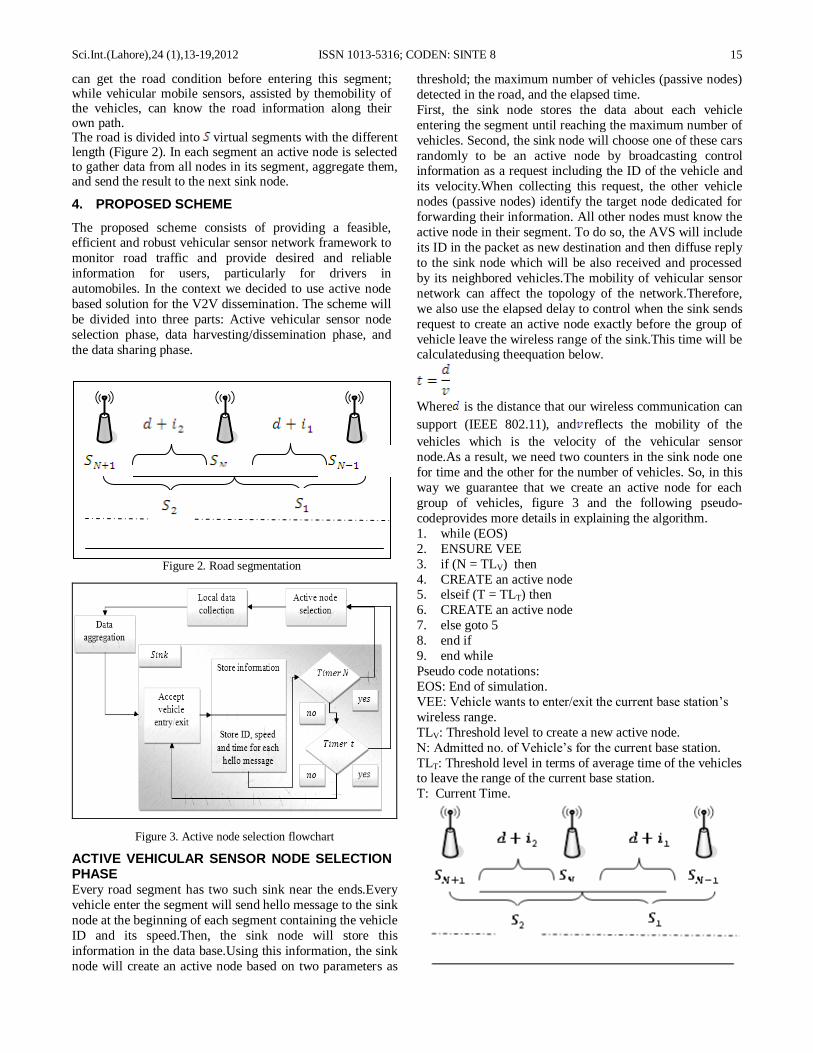
Sci.Int.(Lahore),24 (1),13-19,2012 ISSN 1013-5316; CODEN: SINTE 8
15
can get the road condition before entering this segment; while vehicular mobile sensors, assisted by themobility of the vehicles, can know the road information along their own path. The road is divided into virtual segments with the different length (Figure 2). In each segment an active node is selected to gather data from all nodes in its segment, aggregate them, and send the result to the next sink node.
4. PROPOSED SCHEME
The proposed scheme consists of providing a feasible, efficient and robust vehicular sensor network framework to
monitor road traffic and provide desired and reliable
information for users, particularly for drivers in
automobiles. In the context we decided to use active node
based solution for the V2V dissemination. The scheme will
be divided into three parts: Active vehicular sensor node
selection phase, data harvesting/dissemination phase, and
the data sharing phase.
Figure 2. Road segmentation
Figure 3. Active node selection flowchart
ACTIVE VEHICULAR SENSOR NODE SELECTION PHASE Every road segment has two such sink near the ends.Every
vehicle enter the segment will send hello message to the sink
node at the beginning of each segment containing the vehicle
ID and its speed.Then, the sink node will store this
information in the data base.Using this information, the sink
node will create an active node based on two parameters as
threshold; the maximum number of vehicles (passive nodes)
detected in the road, and the elapsed time.
First, the sink node stores the data about each vehicle
entering the segment until reaching the maximum number of
vehicles. Second, the sink node will choose one of these cars
randomly to be an active node by broadcasting control information as a request including the ID of the vehicle and
its velocity.When collecting this request, the other vehicle
nodes (passive nodes) identify the target node dedicated for
forwarding their information. All other nodes must know the
active node in their segment. To do so, the AVS will include
its ID in the packet as new destination and then diffuse reply
to the sink node which will be also received and processed
by its neighbored vehicles.The mobility of vehicular sensor
network can affect the topology of the network.Therefore,
we also use the elapsed delay to control when the sink sends
request to create an active node exactly before the group of
vehicle leave the wireless range of the sink.This time will be calculatedusing theequation below.
Where is the distance that our wireless communication can
support (IEEE 802.11), and reflects the mobility of the
vehicles which is the velocity of the vehicular sensor
node.As a result, we need two counters in the sink node one
for time and the other for the number of vehicles. So, in this
way we guarantee that we create an active node for each
group of vehicles, figure 3 and the following pseudo-
codeprovides more details in explaining the algorithm.
1. while (EOS)
2. ENSURE VEE
3. if (N = TLV) then
4. CREATE an active node 5. elseif (T = TLT) then
6. CREATE an active node
7. else goto 5
8. end if
9. end while
Pseudo code notations:
EOS: End of simulation.
VEE: Vehicle wants to enter/exit the current base station’s
wireless range.
TLV: Threshold level to create a new active node.
N: Admitted no. of Vehicle’s for the current base station.
TLT: Threshold level in terms of average time of the vehicles to leave the range of the current base station.
T: Current Time.
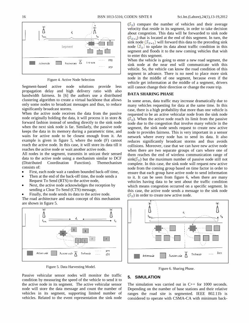
ISSN 1013-5316; CODEN: SINTE 8 Sci.Int.(Lahore),24(1),13-19,2012
16
Figure 4. Active Node Selection
Segment-based active node solutions provide less propagation delay and high delivery ratio with also bandwidth fairness. In [6] the authors use a distributed clustering algorithm to create a virtual backbone that allows only some nodes to broadcast messages and thus, to reduce significantly broadcast storms. When the active node receives the data from the passive node originally holding the data, it will process it in store & forward fashion instead of sending directly to the sink node when the next sink node is far. Similarly, the passive node keeps the data in its memory during a parametric time, and waits for active node to be closest enough from it. An example is given in figure 5, where the node (F) cannot reach the active node. In this case, it will store its data till it reaches the active node or wait another active node. All nodes in the segment, transmits in unicast their sensed data to the active node using a mechanism similar to DCF (Distributed Coordination Function). Themechanism consists of: First, each node wait a random bounded back-off time, Then at the end of the back-off time, the node sends a
Request To Send (RTS) to the active node, Next, the active node acknowledges the reception by
sending a Clear To Send (CTS) message, Finally, the node sends its data to the active node. The road architecture and main concept of this mechanism are shown in figure 5.
Figure 5. Data Harvesting Model.
Passive vehicular sensor nodes will monitor the traffic condition by measuring the speed of the vehicle to send it to the active node in its segment. The active vehicular sensor node will store the data message and count the number of vehicles in its segment, supporting limited number of vehicles. Related to the event representation the sink node
( ) compare the number of vehicles and their average velocity that reside in its segment, in order to take decision about congestion. This data will be forwarded to sink node ( ) that is located at the end of this segment. In turn, the sink node will forward this data to the preceding sink node to update its data about traffic condition in this segment and floods it to the new coming vehicles that wish to enter this segment. When the vehicle is going to enter a new road segment, the sink node at the near end will communicate with this vehicle. So, the vehicle can know the road condition of this segment in advance. There is no need to place more sink node in the middle of one segment, because even if the vehicle get information at the middle of a segment, drivers still cannot change their direction or change the route trip.
DATA SHARING PHASE
In some areas, data traffic may increase dramatically due to many vehicles requesting for data at the same time. In this case, there is a high probability that more than one vehicle is requested to be an active vehicular node from the sink node ( ). When the active node reach its limit from the passive node due to the congestion that involve many vehicle in the segment, the sink node sends request to create new active node to provides fairness. This is very important in a sensor network where every node has to send its data. It also reduces significantly broadcast storms and thus avoids collisions. Moreover, case that we can have new active node when there are two separate groups of cars where one of them reaches the end of wireless communication range of sink( ) but the maximum number of passive node still not complete. In this case, the sink node will request new active node from the coming group based on time factor in order to ensure that each group have active node to send information to it. It can be seen from figure 6, when there are many vehicles having data to be sent about the traffic condition which means congestion occurred on a specific segment. In this case, the active node sends a message to the sink node ( ) in order to create new active node.
Figure 6. Sharing Phase.
5. SIMULATION
The simulation was carried out in C++ for 1000 seconds. Depending on the number of base stations and their relative
ranges the road site is segmented. IEEE 802.11b is
considered to operate with CSMA-CA with minimum back-
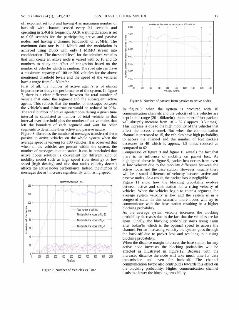
Sci.Int.(Lahore),24 (1),13-19,2012 ISSN 1013-5316; CODEN: SINTE 8
17
off exponent set to 3 and having 4 as maximum number of
back-off with channel sensed every 0.1 seconds and
operating in 2.4GHz frequency, ACK waiting duration is set
to 0.05 seconds for the participating active and passive
nodes, and having a channel bandwidth of 20MHz. The
maximum data rate is 11 Mbit/s and the modulation is achieved using DSSS with only 1 MIMO stream into
consideration. The threshold level for the admitted vehicles
that will create an active node is varied with 5, 10 and 15
numbers to study the effect of congestion based on the
number of vehicles which is random. The road site can have
a maximum capacity of 100 or 200 vehicles for the above
mentioned threshold levels and the speed of the vehicles
have a range from 0-180km/hr. First of all, the number of active agent’s is of utmost importance to study the performance of the system. In figure 7, there is a clear difference between the total number of vehicle that enter the segment and the subsequent active agents. This reflects that the number of messages between the vehicle’s and infrastructure would be reduced to 90%. The total number of active agents/nodes during a given time interval is calculated as number of total vehicle in that interval over threshold plus the number of active nodes that left the boundary of each segment and wait for other segments to determine their active and passive nature. Figure 8 illustrates the number of messages transferred from passive to active vehicles on the whole system when the average speed is varying for 100 vehicles. It is observed that when all the vehicles are present within the system, the number of messages is quite stable. It can be concluded that active nodes solution is convenient for different kind of mobility model such as high speed (low density) or low speed (high density) and also that nodes velocity doesn’t affects the active nodes performance. Indeed, the number of messages doesn’t increase significantly with rising speed.
0 100 200 300 400 500 600 700 800 900 10000
20
40
60
80
100
120
140
160
Time(sec)
Num
ber of V
ehic
les
Number of vehicles vs Time
Total Number of Vehicles
Number of Active Nodes for Nth
=10
Number of Active Nodes for Nth
=5
Number of Active Nodes for Nth
=4
Figure 7. Number of Vehicles vs Time
0 20 40 60 80 100 120 140 160 1804000
4500
5000
5500
6000
6500
7000
7500
8000
Velocity (km/h)
Num
ber
of
Packets
fro
m P
assiv
e t
o A
ctive
Number of Packets vs Velocity for 100 vehicle
Figure 8. Number of packets from passive to active nodes
In figure 9, when the system is procured with 10 communication channels and the velocity of the vehicles are kept in this range (20–160km/hr), the number of lost packets will abruptly increase from 18 – 62 ( approx. 3.5 times). This increase is due to the high mobility of the vehicles that affect the access channel. But when the communication channel is increased to 15, the vehicles have high probability to access the channel and the number of lost packets decreases to 40 which is approx. 1.5 times reduced as compared to 62. Comparison of figure 9 and figure 10 reveals the fact that there is an influence of mobility on packet loss. As highlighted above in figure 9, packet loss occurs from even at low velocity due to the mobility difference between the active nodes and the base station. However, usually there will be a small difference of velocity between active and passive nodes. As a result, the packet loss is negligible. Figure 11 show how the blocking probability evolves between active and sink station for a rising velocity of vehicles. When the vehicles begin to enter a segment, the average system velocity is low and the system is in a congested state. In this scenario, more nodes will try to communicate with the base station resulting in a higher blocking probability. As the average system velocity increases the blocking probability decreases due to the fact that the vehicles are far apart. Finally, the blocking probability starts rising again after 55km/hr which is the optimal speed to access the channel. For an increasing velocity the system goes through the back-off due to packet loss and resulting in a rising blocking probability. When the distance margin to access the base station for any active node increases the blocking probability will be affected as illustrated in figure 12. Because with the increased distance the node will take much time for data transmission and even for back-off. The channel communication factor also contributes towards this effect on the blocking probability. Higher communication channel leads to a lower the blocking probability.
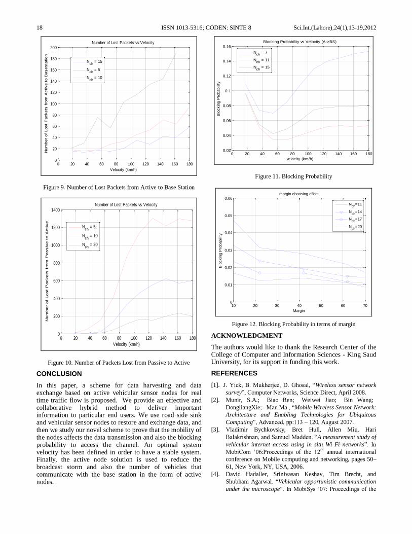
ISSN 1013-5316; CODEN: SINTE 8 Sci.Int.(Lahore),24(1),13-19,2012
18
0 20 40 60 80 100 120 140 160 1800
20
40
60
80
100
120
140
160
180
200
Velocity (km/h)
Num
ber
of
Lost
Packets
fro
m A
ctive t
o B
asesta
tion
Number of Lost Packets vs Velocity
Nch
= 15
Nch
= 5
Nch
= 10
Figure 9. Number of Lost Packets from Active to Base Station
0 20 40 60 80 100 120 140 160 1800
200
400
600
800
1000
1200
1400
Velocity (km/h)
Num
ber
of
Lost
Packets
fro
m P
assiv
e t
o A
ctive
Number of Lost Packets vs Velocity
Nch
= 5
Nch
= 10
Nch
= 20
Figure 10. Number of Packets Lost from Passive to Active
CONCLUSION
In this paper, a scheme for data harvesting and data exchange based on active vehicular sensor nodes for real time traffic flow is proposed. We provide an effective and collaborative hybrid method to deliver important information to particular end users. We use road side sink and vehicular sensor nodes to restore and exchange data, and then we study our novel scheme to prove that the mobility of the nodes affects the data transmission and also the blocking probability to access the channel. An optimal system velocity has been defined in order to have a stable system. Finally, the active node solution is used to reduce the broadcast storm and also the number of vehicles that communicate with the base station in the form of active nodes.
0 20 40 60 80 100 120 140 160 1800.02
0.04
0.06
0.08
0.1
0.12
0.14
0.16
velocity (km/h)
Blo
ckin
g P
robabili
ty
Blocking Probability vs Velocity (A->BS)
Nch
= 7
Nch
= 11
Nch
= 15
Figure 11. Blocking Probability
10 20 30 40 50 60 700
0.01
0.02
0.03
0.04
0.05
0.06
Margin
Blo
ckin
g P
robabili
ty
margin choosing effect
Nch
=11
Nch
=14
Nch
=17
Nch
=20
Figure 12. Blocking Probability in terms of margin
ACKNOWLEDGMENT
The authors would like to thank the Research Center of the College of Computer and Information Sciences - King Saud University, for its support in funding this work.
REFERENCES
[1]. J. Yick, B. Mukherjee, D. Ghosal, “Wireless sensor network
survey”, Computer Networks, Science Direct, April 2008.
[2]. Munir, S.A.; Biao Ren; Weiwei Jiao; Bin Wang;
DongliangXie; Man Ma , “Mobile Wireless Sensor Network:
Architecture and Enabling Technologies for Ubiquitous
Computing”, Advanced, pp:113 – 120, August 2007.
[3]. Vladimir Bychkovsky, Bret Hull, Allen Miu, Hari
Balakrishnan, and Samuel Madden. “A measurement study of
vehicular internet access using in situ Wi-Fi networks”. In
MobiCom ’06:Proceedings of the 12th annual international
conference on Mobile computing and networking, pages 50–
61, New York, NY, USA, 2006.
[4]. David Hadaller, Srinivasan Keshav, Tim Brecht, and
Shubham Agarwal. “Vehicular opportunistic communication
under the microscope”. In MobiSys ’07: Proceedings of the
Sci.Int.(Lahore),24 (1),13-19,2012 ISSN 1013-5316; CODEN: SINTE 8
19
5th international conference on Mobile systems, applications
and services, pages 206–219, New York, NY, USA, 2007.
[5]. J. Ott and D. Kutscher. “Drive-thru internet: IEEE 802.11b
for automobile users”. In 23rd Annual IEEE Conference on
Computer Communications (INFOCOM), 2004.
[6]. I. Salhi, M. O. Cherif, S. M. Senouci, “A New Architecture
for Data Collection in Vehicular Networks”, IEEE
International Conference onCommunications ICC'09, pp.1–6,
August 2009.
[7]. U. Lee, E. Magistretti, B. Zhou, M. Gerla, P. Bellavista, A.
Corradi. “Efficient data harvesting in mobile sensor
platforms”, Proceedings of the 4th annual IEEE International
Conference on Pervasive Computing and Communications
Workshops PERCOMW’06, pp. 352, 2006.
[8]. H. Ng, S.L. Tan, J. G. Guzman, “Road traffic monitoring
using a wireless vehicle sensor network”, International
Symposium on Intelligent Signal Processing and
Communications Systems, ISPACS’08. pp. 1–4, Feb. 2009.
[9]. K.W. Lim Y.-B. Ko, “Multi-hop data harvesting in vehicular
sensor networks”, Communications, IET, Vol.4, no7,
pp.768–775, April 2010.
[10]. Chennikara-Varghese J, Chen W, Hikita T and Onishi
R,“Local peer groups andvehicle-to-infrastructure
communications”. GLOBECOM’07: Proceedings of the
IEEE GlobalTelecommunications Conference – Workshops,
pp. 1–6, 2007.
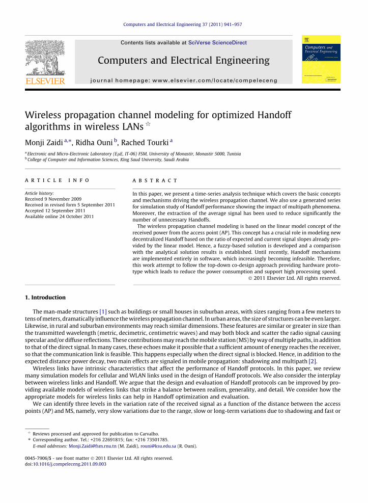
Computers and Electrical Engineering 37 (2011) 941–957
Contents lists available at SciVerse ScienceDirect
Computers and Electrical Engineering
journal homepage: www.elsevier .com/ locate/compeleceng
Wireless propagation channel modeling for optimized Handoffalgorithms in wireless LANs q
Monji Zaidi a,⇑, Ridha Ouni b, Rached Tourki a
a Electronic and Micro-Electronic Laboratory (ElE, IT-06) FSM, University of Monastir, Monastir 5000, Tunisiab College of Computer and Information Sciences, King Saud University, Saudi Arabia
a r t i c l e i n f o
Article history:Received 9 November 2009Received in revised form 5 September 2011Accepted 12 September 2011Available online 24 October 2011
0045-7906/$ - see front matter � 2011 Elsevier Ltddoi:10.1016/j.compeleceng.2011.09.003
q Reviews processed and approved for publication⇑ Corresponding author. Tel.: +216 22691815; fax
E-mail addresses: [email protected] (M. Za
a b s t r a c t
In this paper, we present a time-series analysis technique which covers the basic conceptsand mechanisms driving the wireless propagation channel. We also use a generated seriesfor simulation study of Handoff performance showing the impact of multipath phenomena.Moreover, the extraction of the average signal has been used to reduce significantly thenumber of unnecessary Handoffs.
The wireless propagation channel modeling is based on the linear model concept of thereceived power from the access point (AP). This concept has a crucial role in modeling newdecentralized Handoff based on the ratio of expected and current signal slopes already pro-vided by the linear model. Hence, a fuzzy-based solution is developed and a comparisonwith the analytical solution results is established. Until recently, Handoff mechanismsare implemented entirely in software, which increasingly becoming infeasible. Therefore,this work attempt to follow the top-down co-design approach providing hardware proto-type which leads to reduce the power consumption and support high processing speed.
� 2011 Elsevier Ltd. All rights reserved.
1. Introduction
The man-made structures [1] such as buildings or small houses in suburban areas, with sizes ranging from a few meters totens of meters, dramatically influence the wireless propagation channel. In urban areas, the size of structures can be even larger.Likewise, in rural and suburban environments may reach similar dimensions. These features are similar or greater in size thanthe transmitted wavelength (metric, decimetric, centimetric waves) and may both block and scatter the radio signal causingspecular and/or diffuse reflections. These contributions may reach the mobile station (MS) by way of multiple paths, in additionto that of the direct signal. In many cases, these echoes make it possible that a sufficient amount of energy reaches the receiver,so that the communication link is feasible. This happens especially when the direct signal is blocked. Hence, in addition to theexpected distance power decay, two main effects are signaled in mobile propagation: shadowing and multipath [2].
Wireless links have intrinsic characteristics that affect the performance of Handoff protocols. In this paper, we reviewmany simulation models for cellular and WLAN links used in the design of Handoff protocols. We also consider the interplaybetween wireless links and Handoff. We argue that the design and evaluation of Handoff protocols can be improved by pro-viding available models of wireless links that strike a balance between realism, generality, and detail. We consider how theappropriate models for wireless links can help in Handoff optimization and evaluation.
We can identify three levels in the variation rate of the received signal as a function of the distance between the accesspoints (AP) and MS, namely, very slow variations due to the range, slow or long-term variations due to shadowing and fast or
. All rights reserved.
to Carvalho.: +216 73501785.idi), [email protected] (R. Ouni).
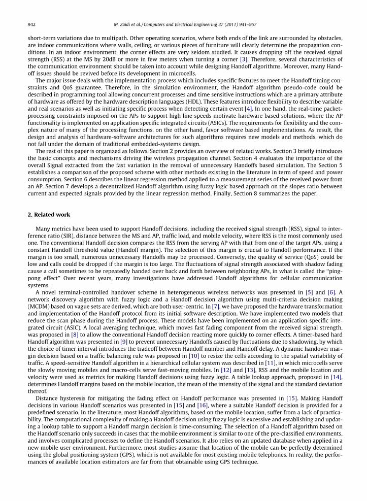
942 M. Zaidi et al. / Computers and Electrical Engineering 37 (2011) 941–957
short-term variations due to multipath. Other operating scenarios, where both ends of the link are surrounded by obstacles,are indoor communications where walls, ceiling, or various pieces of furniture will clearly determine the propagation con-ditions. In an indoor environment, the corner effects are very seldom studied. It causes dropping off the received signalstrength (RSS) at the MS by 20dB or more in few meters when turning a corner [3]. Therefore, several characteristics ofthe communication environment should be taken into account while designing Handoff algorithms. Moreover, many Hand-off issues should be revived before its development in microcells.
The major issue deals with the implementation process which includes specific features to meet the Handoff timing con-straints and QoS guarantee. Therefore, in the simulation environment, the Handoff algorithm pseudo-code could bedescribed in programming tool allowing concurrent processes and time sensitive instructions which are a primary attributeof hardware as offered by the hardware description languages (HDL). These features introduce flexibility to describe variableand real scenarios as well as initiating specific process when detecting certain event [4]. In one hand, the real-time packet-processing constraints imposed on the APs to support high line speeds motivate hardware based solutions, where the APfunctionality is implemented on application specific integrated circuits (ASICs). The requirements for flexibility and the com-plex nature of many of the processing functions, on the other hand, favor software based implementations. As result, thedesign and analysis of hardware-software architectures for such algorithms requires new models and methods, which donot fall under the domain of traditional embedded-systems design.
The rest of this paper is organized as follows. Section 2 provides an overview of related works. Section 3 briefly introducesthe basic concepts and mechanisms driving the wireless propagation channel. Section 4 evaluates the importance of theoverall Signal extracted from the fast variation in the removal of unnecessary Handoffs based simulation. The Section 5establishes a comparison of the proposed scheme with other methods existing in the literature in term of speed and powerconsumption. Section 6 describes the linear regression method applied to a measurement series of the received power froman AP. Section 7 develops a decentralized Handoff algorithm using fuzzy logic based approach on the slopes ratio betweencurrent and expected signals provided by the linear regression method. Finally, Section 8 summarizes the paper.
2. Related work
Many metrics have been used to support Handoff decisions, including the received signal strength (RSS), signal to inter-ference ratio (SIR), distance between the MS and AP, traffic load, and mobile velocity, where RSS is the most commonly usedone. The conventional Handoff decision compares the RSS from the serving AP with that from one of the target APs, using aconstant Handoff threshold value (Handoff margin). The selection of this margin is crucial to Handoff performance. If themargin is too small, numerous unnecessary Handoffs may be processed. Conversely, the quality of service (QoS) could below and calls could be dropped if the margin is too large. The fluctuations of signal strength associated with shadow fadingcause a call sometimes to be repeatedly handed over back and forth between neighboring APs, in what is called the ‘‘ping-pong effect’’ Over recent years, many investigations have addressed Handoff algorithms for cellular communicationsystems.
A novel terminal-controlled handover scheme in heterogeneous wireless networks was presented in [5] and [6]. Anetwork discovery algorithm with fuzzy logic and a Handoff decision algorithm using multi-criteria decision making(MCDM) based on vague sets are derived, which are both user-centric. In [7], we have proposed the hardware transformationand implementation of the Handoff protocol from its initial software description. We have implemented two models thatreduce the scan phase during the Handoff process. These models have been implemented on an application-specific inte-grated circuit (ASIC). A local averaging technique, which moves fast fading component from the received signal strength,was proposed in [8] to allow the conventional Handoff decision reacting more quickly to corner effects. A timer-based hardHandoff algorithm was presented in [9] to prevent unnecessary Handoffs caused by fluctuations due to shadowing, by whichthe choice of timer interval introduces the tradeoff between Handoff number and Handoff delay. A dynamic handover mar-gin decision based on a traffic balancing rule was proposed in [10] to resize the cells according to the spatial variability oftraffic. A speed-sensitive Handoff algorithm in a hierarchical cellular system was described in [11], in which microcells servethe slowly moving mobiles and macro-cells serve fast-moving mobiles. In [12] and [13], RSS and the mobile location andvelocity were used as metrics for making Handoff decisions using fuzzy logic. A table lookup approach, proposed in [14],determines Handoff margins based on the mobile location, the mean of the intensity of the signal and the standard deviationthereof.
Distance hysteresis for mitigating the fading effect on Handoff performance was presented in [15]. Making Handoffdecisions in various Handoff scenarios was presented in [15] and [16], where a suitable Handoff decision is provided for apredefined scenario. In the literature, most Handoff algorithms, based on the mobile location, suffer from a lack of practica-bility. The computational complexity of making a Handoff decision using fuzzy logic is excessive and establishing and updat-ing a lookup table to support a Handoff margin decision is time-consuming. The selection of a Handoff algorithm based onthe Handoff scenario only succeeds in cases that the mobile environment is similar to one of the pre-classified environments,and involves complicated processes to define the Handoff scenarios. It also relies on an updated database when applied in anew mobile user environment. Furthermore, most studies assume that location of the mobile can be perfectly determinedusing the global positioning system (GPS), which is not available for most existing mobile telephones. In reality, the perfor-mances of available location estimators are far from that obtainable using GPS technique.
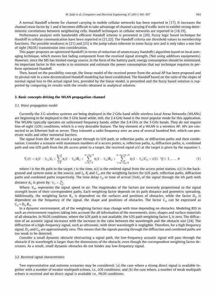
M. Zaidi et al. / Computers and Electrical Engineering 37 (2011) 941–957 943
A normal Handoff scheme for channel carrying in mobile cellular networks has been reported in [17]. It increases thechannel reuse factor by 1 and it becomes difficult to take advantage of channel carrying if traffic were to exhibit strong deter-ministic correlations between neighboring cells. Handoff techniques in cellular networks are reported in [18,19].
Performance analysis with bandwidth efficient Handoff scheme is presented in [20]. Fuzzy logic based technique forHandoff in cellular communication have been reported in [21,22]. The Handoff criteria use threshold values to membershipfunctions. The possible weakness in [21] and [23] is the jump values inherent in some fuzzy sets and it only takes a non lineof sight (NLOS) transmission into consideration.
This paper proposes an optimized Handoff (in terms of reduction of unnecessary Handoffs) algorithm based on local aver-aging technique, which moves fast fading component from the received signal strength. (Not using additives equipments).However, since the MS has limited energy source, in the form of the battery pack, energy consumption should be minimized.An important factor in this works is to minimize and estimate the power consumption that our technique requires to per-form optimized Handoff.
Then, based on the possibility concept, the linear model of the received power from the actual AP has been proposed andits pivotal role in a new decentralized Handoff modeling has been established. The Handoff based on the ratio of the slopes ofnormal signal loss to the actual signal loss, provided by the linear model, is presented and the fuzzy based solution is sup-ported by comparing its results with the results obtained in analytical solution.
3. Basic concepts driving the WLAN propagation channel
3.1. Wave propagation model
Currently the 3 G wireless systems are being deployed in the 2 GHz band while wireless Local Areas Networks (WLANs)are beginning to be deployed in the 5 GHz band while, still, the 2.4 GHz band is the most popular mode for this application.The WLANs typically operates on unlicensed frequency bands, either the 2.4 GHz or the 5 GHz bands. They do not requireline-of-sight (LOS) conditions, which is a very desirable feature. The key element of a WLAN is a wireless AP. APs are con-nected to an Ethernet hub or server. They transmit a radio frequency over an area of several hundred feet, which can pen-etrate walls and other nonmetal barriers.
The signal from the AP can reach a target through its LOS path, or reflection paths, or diffraction paths and their combi-nation. Consider a scenario with maximum numbers of n access points, nr reflection paths, nd diffraction paths, nc combinedpath and one LOS path from the jth access point to a target, the received signal y(t) at the target is given by the equation 1.
YjðtÞ ¼ xjðt � s1;jÞLj þXnrþ2
i¼2
xjðt � si;jÞRi;j þXnrþndþ3
i¼nrþ3
xjðt � si;jÞRi;j þXnrþndþncþ4
i¼nrþndþ4
xjðt � si;jÞCi;j þ eðtÞ; 8j 2 1; . . . ; n ð1Þ
where i is the ith path to the target, t is the time, x(t) is the emitted signal from the access point station, e(t) is the back-ground and system noise at the source, and Lj, Rj and Ci,j are the weighting factors for LOS path, reflection paths, diffractionpaths and combined paths respectively. The time delay si,j or time of arrival (ToA), of the signal through the ith path with
distance di,j is given by: si;j ¼di;j
Vair.
Where, Vair represents the signal speed in air. The magnitudes of the factors are inversely proportional to the signalstrength losses of their correspondent paths. Each weighting factor depends on its path distance and geometric spreading.Additionally, the weighting factor Ri,j is dependent on the surfaces and positions of obstacles, while the factor Di,j isdependent on the frequency of the signal, the shape and positions of obstacles. The factor Ci,j can be expressed asCi,j = Di,j�Ri,j.
In a dynamic environment, all of the weighting factors may change with time depending on obstacles. Modeling RSS insuch an environment requires taking into account the all information of the movements, sizes, shapes and surface materialsof all obstacles. In NLOS conditions, where the LOS path is not available, the LOS path weighting factor Lj is zero. The diffrac-tion of an acoustic signal increases with the increase in the ratio between the wavelength and the obstacle size [24]. Thediffraction of a high-frequency signal, such as ultrasonic, with short wavelength is negligible. Therefore, for a high frequencysignal, Di,j and Ci,j are approximately zero. This means that the signals passing through the diffraction and combined paths aretoo weak to be detected.
Consider a small dynamic obstacle obstructing a signal path, the low-frequency acoustic signal will pass through theobstacle if its wavelength is larger than the dimensions of the obstacle, even though the correspondent weighting factor de-creases. As a result, small dynamic obstacles do not hinder any low-frequency signal.
3.2. Received signal characteristics
Two representative and extreme scenarios may be considered: (a) the case where a strong direct signal is available to-gether with a number of weaker multipath echoes, i.e., LOS conditions; and (b) the case where, a number of weak multipathechoes is received and no direct signal is available i.e., NLOS conditions.
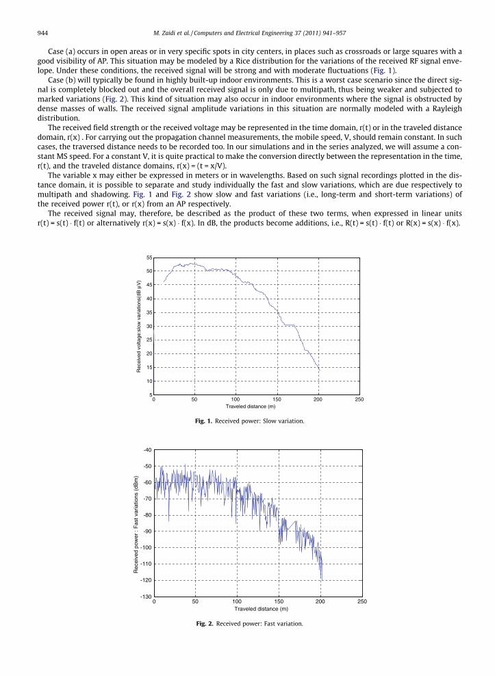
944 M. Zaidi et al. / Computers and Electrical Engineering 37 (2011) 941–957
Case (a) occurs in open areas or in very specific spots in city centers, in places such as crossroads or large squares with agood visibility of AP. This situation may be modeled by a Rice distribution for the variations of the received RF signal enve-lope. Under these conditions, the received signal will be strong and with moderate fluctuations (Fig. 1).
Case (b) will typically be found in highly built-up indoor environments. This is a worst case scenario since the direct sig-nal is completely blocked out and the overall received signal is only due to multipath, thus being weaker and subjected tomarked variations (Fig. 2). This kind of situation may also occur in indoor environments where the signal is obstructed bydense masses of walls. The received signal amplitude variations in this situation are normally modeled with a Rayleighdistribution.
The received field strength or the received voltage may be represented in the time domain, r(t) or in the traveled distancedomain, r(x) . For carrying out the propagation channel measurements, the mobile speed, V, should remain constant. In suchcases, the traversed distance needs to be recorded too. In our simulations and in the series analyzed, we will assume a con-stant MS speed. For a constant V, it is quite practical to make the conversion directly between the representation in the time,r(t), and the traveled distance domains, r(x) = (t = x/V).
The variable x may either be expressed in meters or in wavelengths. Based on such signal recordings plotted in the dis-tance domain, it is possible to separate and study individually the fast and slow variations, which are due respectively tomultipath and shadowing. Fig. 1 and Fig. 2 show slow and fast variations (i.e., long-term and short-term variations) ofthe received power r(t), or r(x) from an AP respectively.
The received signal may, therefore, be described as the product of these two terms, when expressed in linear unitsr(t) = s(t) � f(t) or alternatively r(x) = s(x) � f(x). In dB, the products become additions, i.e., R(t) = s(t) � f(t) or R(x) = s(x) � f(x).
0 50 100 150 200 2505
10
15
20
25
30
35
40
45
50
55
Rec
eive
d vo
ltage
:slo
w v
aria
tions
(dB
μV
)
Traveled distance (m)
Fig. 1. Received power: Slow variation.
0 50 100 150 200 250-130
-120
-110
-100
-90
-80
-70
-60
-50
-40
Rec
eive
d po
wer
: F
ast v
aria
tions
(dB
m)
Traveled distance (m)
Fig. 2. Received power: Fast variation.
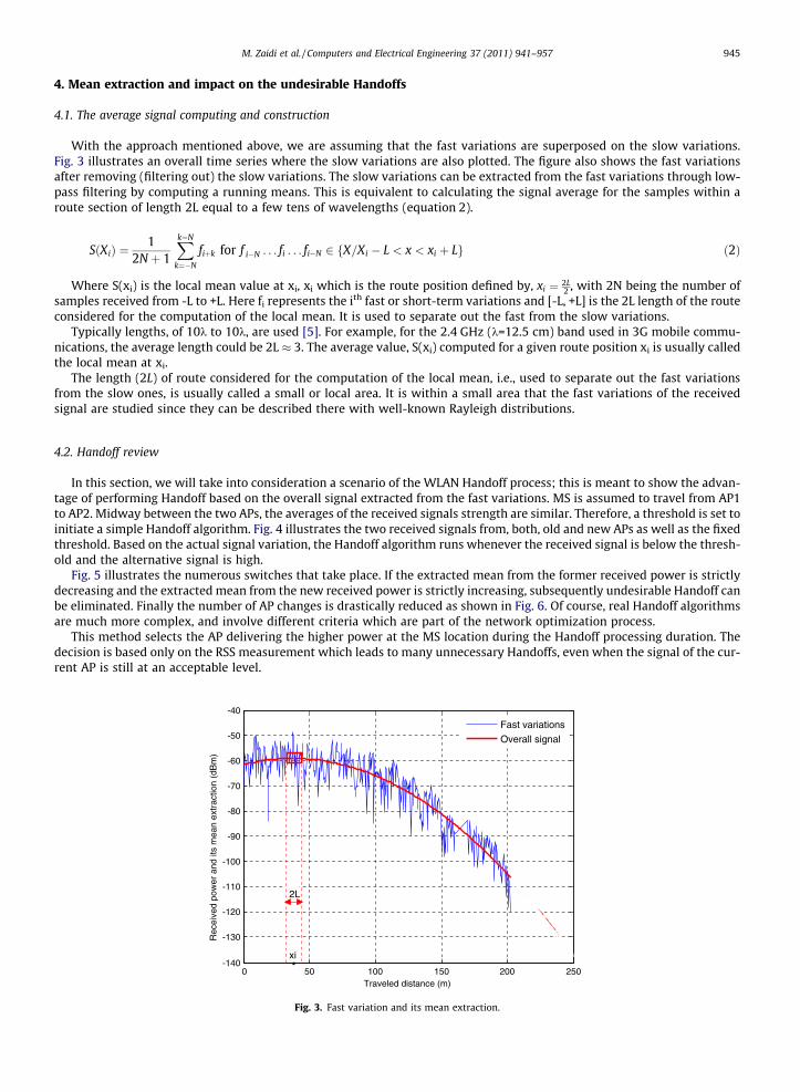
M. Zaidi et al. / Computers and Electrical Engineering 37 (2011) 941–957 945
4. Mean extraction and impact on the undesirable Handoffs
4.1. The average signal computing and construction
With the approach mentioned above, we are assuming that the fast variations are superposed on the slow variations.Fig. 3 illustrates an overall time series where the slow variations are also plotted. The figure also shows the fast variationsafter removing (filtering out) the slow variations. The slow variations can be extracted from the fast variations through low-pass filtering by computing a running means. This is equivalent to calculating the signal average for the samples within aroute section of length 2L equal to a few tens of wavelengths (equation 2).
SðXiÞ ¼1
2N þ 1
Xk¼N
k¼�N
fiþk for f i�N . . . fi . . . fi�N 2 fX=Xi � L < x < xi þ Lg ð2Þ
Where S(xi) is the local mean value at xi, xi which is the route position defined by, xi ¼ 2L2 , with 2N being the number of
samples received from -L to +L. Here fi represents the ith fast or short-term variations and [-L, +L] is the 2L length of the routeconsidered for the computation of the local mean. It is used to separate out the fast from the slow variations.
Typically lengths, of 10k to 10k, are used [5]. For example, for the 2.4 GHz (k=12.5 cm) band used in 3G mobile commu-nications, the average length could be 2L � 3. The average value, S(xi) computed for a given route position xi is usually calledthe local mean at xi.
The length (2L) of route considered for the computation of the local mean, i.e., used to separate out the fast variationsfrom the slow ones, is usually called a small or local area. It is within a small area that the fast variations of the receivedsignal are studied since they can be described there with well-known Rayleigh distributions.
4.2. Handoff review
In this section, we will take into consideration a scenario of the WLAN Handoff process; this is meant to show the advan-tage of performing Handoff based on the overall signal extracted from the fast variations. MS is assumed to travel from AP1to AP2. Midway between the two APs, the averages of the received signals strength are similar. Therefore, a threshold is set toinitiate a simple Handoff algorithm. Fig. 4 illustrates the two received signals from, both, old and new APs as well as the fixedthreshold. Based on the actual signal variation, the Handoff algorithm runs whenever the received signal is below the thresh-old and the alternative signal is high.
Fig. 5 illustrates the numerous switches that take place. If the extracted mean from the former received power is strictlydecreasing and the extracted mean from the new received power is strictly increasing, subsequently undesirable Handoff canbe eliminated. Finally the number of AP changes is drastically reduced as shown in Fig. 6. Of course, real Handoff algorithmsare much more complex, and involve different criteria which are part of the network optimization process.
This method selects the AP delivering the higher power at the MS location during the Handoff processing duration. Thedecision is based only on the RSS measurement which leads to many unnecessary Handoffs, even when the signal of the cur-rent AP is still at an acceptable level.
0 50 100 150 200 250-140
-130
-120
-110
-100
-90
-80
-70
-60
-50
-40
Rec
eive
d po
wer
and
its
mea
n ex
trac
tion
(dB
m)
Traveled distance (m)
Fast variations
Overall signal
2L
xi
Fig. 3. Fast variation and its mean extraction.
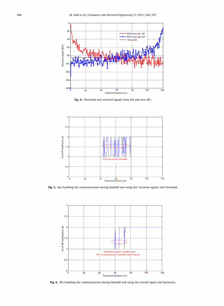
Fig. 4. Threshold and received signals from old and new APs.
Fig. 5. Aps handling the communication during Handoff and using fast variation signals and threshold.
Fig. 6. APs handling the communication during Handoff and using the overall signal and hysteresis.
946 M. Zaidi et al. / Computers and Electrical Engineering 37 (2011) 941–957
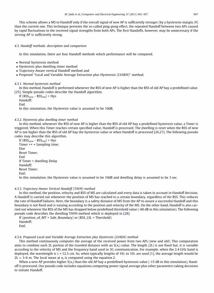
M. Zaidi et al. / Computers and Electrical Engineering 37 (2011) 941–957 947
This scheme allows a MS to Handoff only if the overall signal of new AP is sufficiently stronger (by a hysteresis margin, H)than the current one. This technique prevents the so-called ping-pong effect, the repeated Handoff between two APs causedby rapid fluctuations in the received signal strengths from both APs. The first Handoffs, however, may be unnecessary if theserving AP is sufficiently strong.
4.3. Handoff methods: description and comparison
In this simulation, there are four Handoff methods which performance will be compared.
� Normal hysteresis method� Hysteresis plus dwelling timer method� Trajectory-Aware vertical Handoff method and� Proposed ‘‘Local and Variable Average Extraction plus Hysteresis (LVAEH)’’ method.
4.3.1. Normal hysteresis methodIn this method, Handoff is performed whenever the RSS of new AP is higher than the RSS of old AP bay a predefined value.
[25]. Simple pseudo codes describe the Handoff algorithm.If (RSSnew - RSSold) > HysHandoff;End.In this simulation, the Hysteresis value is assumed to be 10dB.
4.3.2. Hysteresis plus dwelling timer methodIn this method, whenever the RSS of new AP is higher than the RSS of old AP bay a predefined hysteresis value, a Timer is
triggered. When this Timer reaches certain specified value, Handoff is processed. The dwelling is reset when the RSS of newAP is not higher than the RSS of old AP bay the hysteresis value or when Handoff is processed [26,27]. The following pseudocodes may describe this algorithm.
If (RSSnew - RSSold) > HysTimer ++ = Sampling time;ElseReset Timer;EndIf Timer > dwelling DelayHandoff;Reset Timer;End;In this simulation, the Hysteresis value is assumed to be 10dB and dwelling delay is assumed to be 3 sec.
4.3.3. Trajectory-Aware Vertical Handoff (TAVH) methodIn this method, the position, velocity and RSS of MS are calculated and every data is taken in account in Handoff decision.
A Handoff is carried out whenever the position of MS has reached to a certain boundary, regardless of the RSS. This reducesthe rate of Handoff failures. Here, the boundary is a safety distance of MS from the AP to assure a successful Handoff and thisboundary is not fixed and is varying according to the position and velocity of the MS. On the other hand, Handoff is also car-ried out whenever the RSS of the MS has dropped below predefined threshold value (-60 dB in this simulation). The followingpseudo code describes the dwelling TAVH method which is deployed in [28].
If (position_of_MT > Safe_Boundary) or (RSS_LSL < Thershold)Handoff;End;
4.3.4. Proposed Local and Variable Average Extraction plus Hysteresis (LVAEH) methodThis method continuously computes the average of the received power from two APs (new and old). This computation
aims to combine each 2L portion of the traveled distance with an S(xi) value. The length (2L) is not fixed but, it is variableaccording to the velocity of MS and the frequency band used in 3G communication. For example, when the 2.4 GHz band isdeployed, the wavelength is k = 12.5 cm. So, when typically lengths of 10k to 10k are used [1], the average length would be2L � 3-6 m. The local mean at xi is computed using the equation 2.
When a new AP provides higher S(xi) than the old AP bay a predefined hysteresis value (-15 dB in this simulation), Hand-off is processed. Our pseudo code includes equations computing power signal average plus other parameters taking decisionsto initiate Handoff.
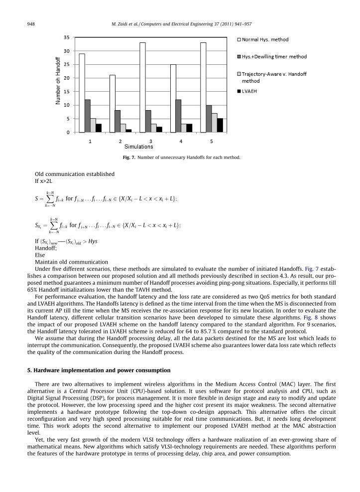
Fig. 7. Number of unnecessary Handoffs for each method.
948 M. Zaidi et al. / Computers and Electrical Engineering 37 (2011) 941–957
Old communication establishedIf x>2L
S ¼Xk¼N
k¼�N
fiþk for f i�N . . . fi . . . fi�N 2 fX=Xi � L < x < xi þ Lg;
SXi¼Xk¼N
k¼�N
fiþk for f iþN . . . fi . . . fi�N 2 fX=Xi � L < x < xi þ Lg;
If ðSXiÞnew——ðSXi
Þold > HysHandoff;ElseMaintain old communicationUnder five different scenarios, these methods are simulated to evaluate the number of initiated Handoffs. Fig. 7 estab-
lishes a comparison between our proposed solution and all methods previously described in section 4.3. As result, our pro-posed method guarantees a minimum number of Handoff processes avoiding ping-pong situations. Especially, it performs till65% Handoff initializations lower than the TAVH method.
For performance evaluation, the handoff latency and the loss rate are considered as two QoS metrics for both standardand LVAEH algorithms. The Handoffs latency is defined as the time interval from the time when the MS is disconnected fromits current AP till the time when the MS receives the re-association response for its new location. In order to evaluate theHandoff latency, different cellular transition scenarios have been developed to simulate these algorithms. Fig. 8 showsthe impact of our proposed LVAEH scheme on the handoff latency compared to the standard algorithm. For 9 scenarios,the Handoff latency tolerated in LVAEH scheme is reduced for 64 to 85.7 % compared to the standard protocol.
We assume that during the Handoff processing delay, all the data packets destined for the MS are lost which leads tointerrupt the communication. Consequently, the proposed LVAEH scheme also guarantees lower data loss rate which reflectsthe quality of the communication during the Handoff process.
5. Hardware implementation and power consumption
There are two alternatives to implement wireless algorithms in the Medium Access Control (MAC) layer. The firstalternative is a Central Processor Unit (CPU)-based solution. It uses software for protocol analysis and CPU, such asDigital Signal Processing (DSP), for process management. It is more flexible in design stage and easy to modify and updatethe protocol. However, the low processing speed and the higher cost present its major weakness. The second alternativeimplements a hardware prototype following the top-down co-design approach. This alternative offers the circuitreconfiguration and very high speed processing suitable for real time communications. But, it needs long developmenttime. This work adopts the second alternative to implement our proposed LVAEH method at the MAC abstractionlevel.
Yet, the very fast growth of the modern VLSI technology offers a hardware realization of an ever-growing share ofmathematical means. New algorithms which satisfy VLSI-technology requirements are needed. These algorithms performthe features of the hardware prototype in terms of processing delay, chip area, and power consumption.
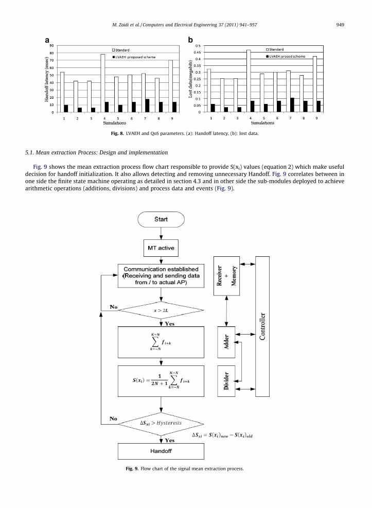
Fig. 8. LVAEH and QoS parameters. (a): Handoff latency, (b): lost data.
M. Zaidi et al. / Computers and Electrical Engineering 37 (2011) 941–957 949
5.1. Mean extraction Process: Design and implementation
Fig. 9 shows the mean extraction process flow chart responsible to provide S(xi) values (equation 2) which make usefuldecision for handoff initialization. It also allows detecting and removing unnecessary Handoff. Fig. 9 correlates between inone side the finite state machine operating as detailed in section 4.3 and in other side the sub-modules deployed to achievearithmetic operations (additions, divisions) and process data and events (Fig. 9).
Fig. 9. Flow chart of the signal mean extraction process.
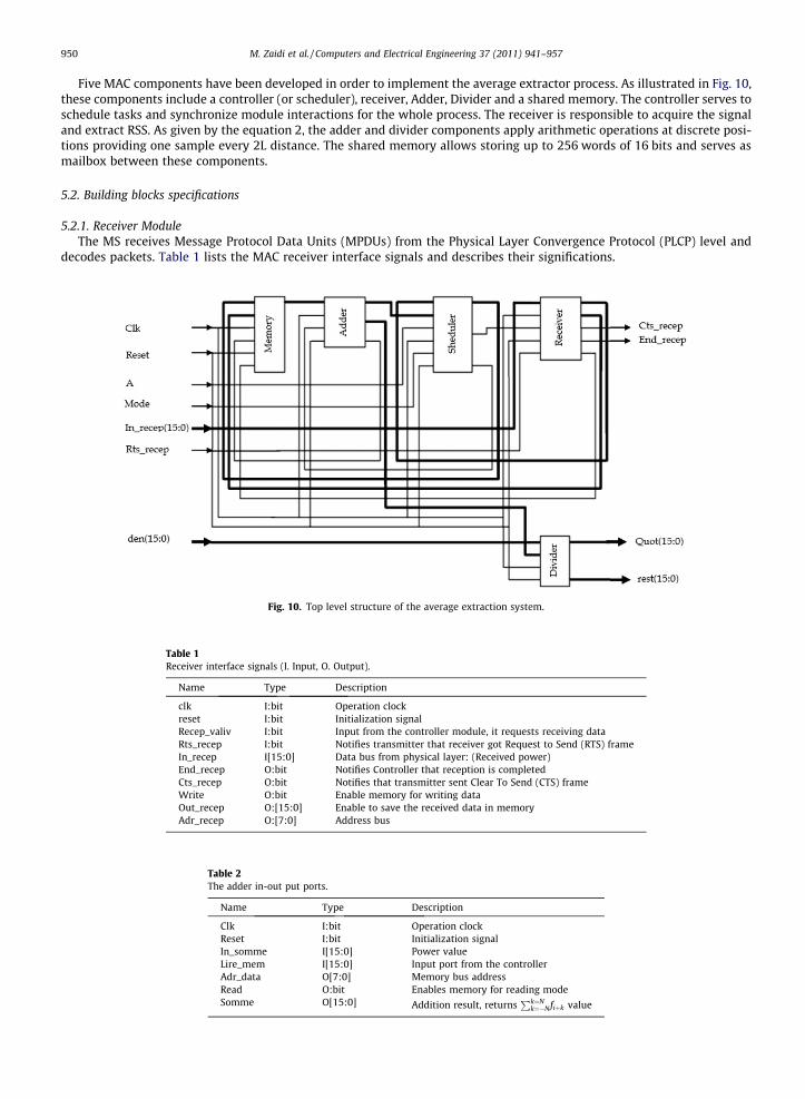
950 M. Zaidi et al. / Computers and Electrical Engineering 37 (2011) 941–957
Five MAC components have been developed in order to implement the average extractor process. As illustrated in Fig. 10,these components include a controller (or scheduler), receiver, Adder, Divider and a shared memory. The controller serves toschedule tasks and synchronize module interactions for the whole process. The receiver is responsible to acquire the signaland extract RSS. As given by the equation 2, the adder and divider components apply arithmetic operations at discrete posi-tions providing one sample every 2L distance. The shared memory allows storing up to 256 words of 16 bits and serves asmailbox between these components.
5.2. Building blocks specifications
5.2.1. Receiver ModuleThe MS receives Message Protocol Data Units (MPDUs) from the Physical Layer Convergence Protocol (PLCP) level and
decodes packets. Table 1 lists the MAC receiver interface signals and describes their significations.
Fig. 10. Top level structure of the average extraction system.
Table 1Receiver interface signals (I. Input, O. Output).
Name Type Description
clk I:bit Operation clockreset I:bit Initialization signalRecep_valiv I:bit Input from the controller module, it requests receiving dataRts_recep I:bit Notifies transmitter that receiver got Request to Send (RTS) frameIn_recep I[15:0] Data bus from physical layer: (Received power)End_recep O:bit Notifies Controller that reception is completedCts_recep O:bit Notifies that transmitter sent Clear To Send (CTS) frameWrite O:bit Enable memory for writing dataOut_recep O:[15:0] Enable to save the received data in memoryAdr_recep O:[7:0] Address bus
Table 2The adder in-out put ports.
Name Type Description
Clk I:bit Operation clockReset I:bit Initialization signalIn_somme I[15:0] Power valueLire_mem I[15:0] Input port from the controllerAdr_data O[7:0] Memory bus addressRead O:bit Enables memory for reading modeSomme O[15:0] Addition result, returns
Pk¼Nk¼�Nfiþk value
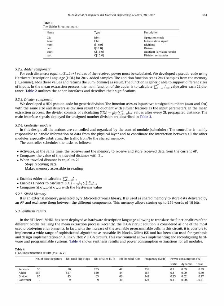
Table 3The divider in-out put ports.
Name Type Description
Clk I:bit Operation clockReset I:bit Initialization signalnum I[15:0] Dividendden I[15:0] Divisorquot O[15:0] Quotient (division result)rest O[15:0] Division remainder
M. Zaidi et al. / Computers and Electrical Engineering 37 (2011) 941–957 951
5.2.2. Adder componentFor each distance x equal to 2L, 2n+1 values of the received power must be calculated. We developed a pseudo-code using
Hardware Description Language (HDL) for 2n+1 added samples. The addition function reads 2n+1 samples from the memory(in_somme), adds these values and returns the Sum (Somme) as result. The function is generic able to support different sizesof inputs. In the mean extraction process, the main function of the adder is to calculate
PNk¼�N f iþk value after each 2L dis-
tance. Table 2 outlines the adder interfaces and describes their significations.
5.2.3. Divider componentWe developed a HDL pseudo-code for generic division. The function uses as inputs two unsigned numbers (num and den)
with the same size and delivers as division result the quotient with similar features as the input parameters. In the meanextraction process, the divider consists of calculating SðXiÞ ¼ 1
2Nþ1
PNk¼�Nfiþk values after every 2L propagated distance. The
main interface signals deployed for unsigned number division are described in Table 3.
5.2.4. Controller moduleIn this design, all the actions are controlled and organized by the control module (scheduler). The controller is mainly
responsible to handle information or data from the physical layer and to coordinate the interaction between all the othermodules especially arbitrating the traffic from/to the shared memory.
The controller schedules the tasks as follows:
� Activates, at the same time, the receiver and the memory to receive and store received data from the current AP.� Compares the value of the traveled distance with 2L.� When traveled distance is equal to 2L
Table 4FPGA Im
ReceAddeDividCont
Stops receiving dataMakes memory accessible in reading
� Enables Adder to calculatePN
k¼�Nfiþk
� Enables Divider to calculate SðXiÞ ¼ 12Nþ1
Pk¼Nk¼�Nfiþk
� Compares S(xi)new-S(xi)odd with the Hysteresis value
5.2.5. SRAM MemoryIt is an external memory generated by STMicroelectronics library. It is used as shared memory to store data delivered by
an AP and exchange them between the different components. This memory allows storing up to 256 words of 16 bits.
5.3. Synthesis results
In the RTL level, VHDL has been deployed as hardware description language allowing to translate the functionalities of thedifferent blocks realizing the mean extraction process. Recently, the FPGA circuit solution is considered as one of the mostused prototyping environments. In fact, with the increase of the available programmable cells in this circuit, it is possible toimplement a wide range of sophisticated algorithms as reusable IPs blocks. Xilinx ISE tool has been also used for synthesisand design implementation on Xilinx Virtex V FPGA circuits. This environment allows implementing and reconfiguring hard-ware and programmable systems. Table 4 shows synthesis results and power consumption estimations for all modules.
plementation results (VIRTEX V).
Nb. of Slice Registers Nb. used Flip Flops Nb. of Slice LUTs Nb. bonded IOBs Frequency (MHz) Power consumption (W)
static dynamic Total
iver 50 50 235 47 238 0.3 0.09 0.39r 557 557 539 44 157 0.4 0.09 0.49er 85 85 63 66 342 0.25 0.02 0.27
roller 9 9 9 30 424 0.3 0.009 �0.31
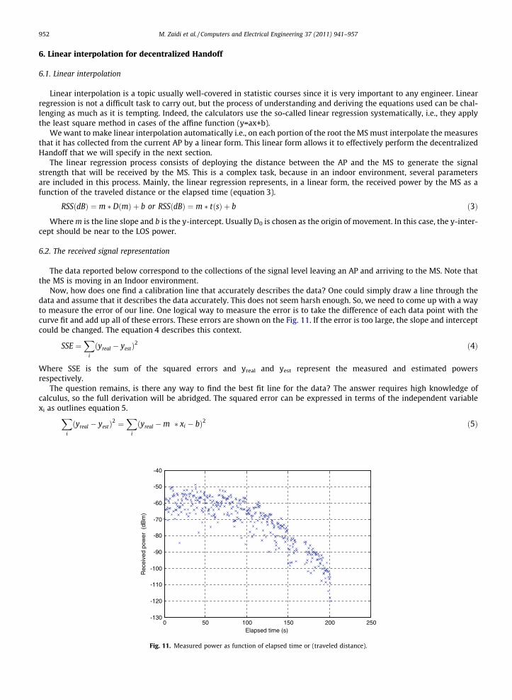
952 M. Zaidi et al. / Computers and Electrical Engineering 37 (2011) 941–957
6. Linear interpolation for decentralized Handoff
6.1. Linear interpolation
Linear interpolation is a topic usually well-covered in statistic courses since it is very important to any engineer. Linearregression is not a difficult task to carry out, but the process of understanding and deriving the equations used can be chal-lenging as much as it is tempting. Indeed, the calculators use the so-called linear regression systematically, i.e., they applythe least square method in cases of the affine function (y=ax+b).
We want to make linear interpolation automatically i.e., on each portion of the root the MS must interpolate the measuresthat it has collected from the current AP by a linear form. This linear form allows it to effectively perform the decentralizedHandoff that we will specify in the next section.
The linear regression process consists of deploying the distance between the AP and the MS to generate the signalstrength that will be received by the MS. This is a complex task, because in an indoor environment, several parametersare included in this process. Mainly, the linear regression represents, in a linear form, the received power by the MS as afunction of the traveled distance or the elapsed time (equation 3).
RSSðdBÞ ¼ m � DðmÞ þ b or RSSðdBÞ ¼ m � tðsÞ þ b ð3Þ
Where m is the line slope and b is the y-intercept. Usually D0 is chosen as the origin of movement. In this case, the y-inter-cept should be near to the LOS power.
6.2. The received signal representation
The data reported below correspond to the collections of the signal level leaving an AP and arriving to the MS. Note thatthe MS is moving in an Indoor environment.
Now, how does one find a calibration line that accurately describes the data? One could simply draw a line through thedata and assume that it describes the data accurately. This does not seem harsh enough. So, we need to come up with a wayto measure the error of our line. One logical way to measure the error is to take the difference of each data point with thecurve fit and add up all of these errors. These errors are shown on the Fig. 11. If the error is too large, the slope and interceptcould be changed. The equation 4 describes this context.
SSE ¼X
i
ðyreal � yestÞ2 ð4Þ
Where SSE is the sum of the squared errors and yreal and yest represent the measured and estimated powersrespectively.
The question remains, is there any way to find the best fit line for the data? The answer requires high knowledge ofcalculus, so the full derivation will be abridged. The squared error can be expressed in terms of the independent variablexi as outlines equation 5.
X
i
ðyreal � yestÞ2 ¼
X
i
ðyreal �m � xi � bÞ2 ð5Þ
0 50 100 150 200 250-130
-120
-110
-100
-90
-80
-70
-60
-50
-40
Rec
eive
d po
wer
(dB
m)
Elapsed time (s)
Fig. 11. Measured power as function of elapsed time or (traveled distance).
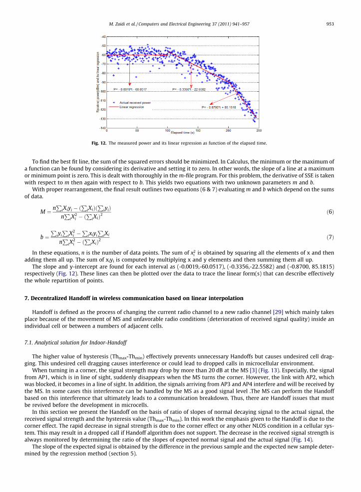
Fig. 12. The measured power and its linear regression as function of the elapsed time.
M. Zaidi et al. / Computers and Electrical Engineering 37 (2011) 941–957 953
To find the best fit line, the sum of the squared errors should be minimized. In Calculus, the minimum or the maximum ofa function can be found by considering its derivative and setting it to zero. In other words, the slope of a line at a maximumor minimum point is zero. This is dealt with thoroughly in the m-file program. For this problem, the derivative of SSE is takenwith respect to m then again with respect to b. This yields two equations with two unknown parameters m and b.
With proper rearrangement, the final result outlines two equations (6 & 7) evaluating m and b which depend on the sumsof data.
M ¼ nP
iXiyi � ðP
iXiÞðP
iyiÞnP
iX2i � ð
PiXiÞ2
ð6Þ
b ¼P
iyi
PiX
2i �
Pixiyi
PiXi
nP
iX2i � ð
PiXiÞ2
ð7Þ
In these equations, n is the number of data points. The sum of x2i is obtained by squaring all the elements of x and then
adding them all up. The sum of xiyi is computed by multiplying x and y elements and then summing them all up.The slope and y-intercept are found for each interval as (-0.0019,-60.0517), (-0.3356,-22.5582) and (-0.8700, 85.1815)
respectively (Fig. 12). These lines can then be plotted over the data to trace the linear form(s) that can describe effectivelythe whole repartition of points.
7. Decentralized Handoff in wireless communication based on linear interpolation
Handoff is defined as the process of changing the current radio channel to a new radio channel [29] which mainly takesplace because of the movement of MS and unfavorable radio conditions (deterioration of received signal quality) inside anindividual cell or between a numbers of adjacent cells.
7.1. Analytical solution for Indoor-Handoff
The higher value of hysteresis (Thmax-Thmin) effectively prevents unnecessary Handoffs but causes undesired cell drag-ging. This undesired cell dragging causes interference or could lead to dropped calls in microcellular environment.
When turning in a corner, the signal strength may drop by more than 20 dB at the MS [3] (Fig. 13). Especially, the signalfrom AP1, which is in line of sight, suddenly disappears when the MS turns the corner. However, the link with AP2, whichwas blocked, it becomes in a line of sight. In addition, the signals arriving from AP3 and AP4 interfere and will be received bythe MS. In some cases this interference can be handled by the MS as a good signal level .The MS can perform the Handoffbased on this interference that ultimately leads to a communication breakdown. Thus, there are Handoff issues that mustbe revived before the development in microcells.
In this section we present the Handoff on the basis of ratio of slopes of normal decaying signal to the actual signal, thereceived signal strength and the hysteresis value (Thmax-Thmin). In this work the emphasis given to the Handoff is due to thecorner effect. The rapid decrease in signal strength is due to the corner effect or any other NLOS condition in a cellular sys-tem. This may result in a dropped call if Handoff algorithm does not support. The decrease in the received signal strength isalways monitored by determining the ratio of the slopes of expected normal signal and the actual signal (Fig. 14).
The slope of the expected signal is obtained by the difference in the previous sample and the expected new sample deter-mined by the regression method (section 5).
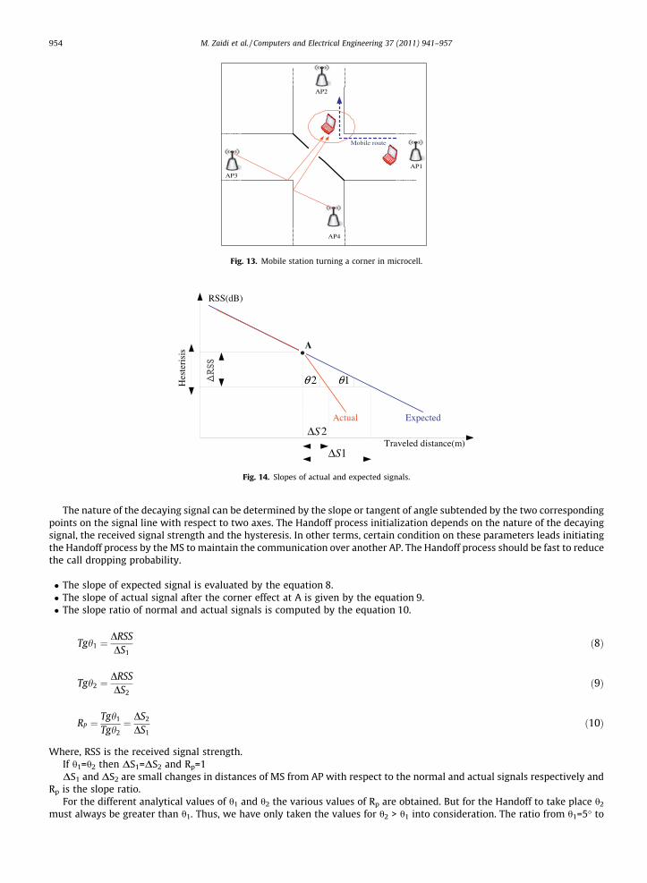
ExpectedActual
1θ
1SΔ
2SΔ
RSS(dB)
Traveled distance(m)
Hes
teri
sis
2θ
A
Fig. 14. Slopes of actual and expected signals.
AP3
AP1
AP2
AP4
Mobile route
Fig. 13. Mobile station turning a corner in microcell.
954 M. Zaidi et al. / Computers and Electrical Engineering 37 (2011) 941–957
The nature of the decaying signal can be determined by the slope or tangent of angle subtended by the two correspondingpoints on the signal line with respect to two axes. The Handoff process initialization depends on the nature of the decayingsignal, the received signal strength and the hysteresis. In other terms, certain condition on these parameters leads initiatingthe Handoff process by the MS to maintain the communication over another AP. The Handoff process should be fast to reducethe call dropping probability.
� The slope of expected signal is evaluated by the equation 8.� The slope of actual signal after the corner effect at A is given by the equation 9.� The slope ratio of normal and actual signals is computed by the equation 10.
Tgh1 ¼DRSSDS1
ð8Þ
Tgh2 ¼DRSSDS2
ð9Þ
RP ¼Tgh1
Tgh2¼ DS2
DS1ð10Þ
Where, RSS is the received signal strength.If h1=h2 then DS1=DS2 and Rp=1DS1 and DS2 are small changes in distances of MS from AP with respect to the normal and actual signals respectively and
Rp is the slope ratio.For the different analytical values of h1 and h2 the various values of Rp are obtained. But for the Handoff to take place h2
must always be greater than h1. Thus, we have only taken the values for h2 > h1 into consideration. The ratio from h1=5� to
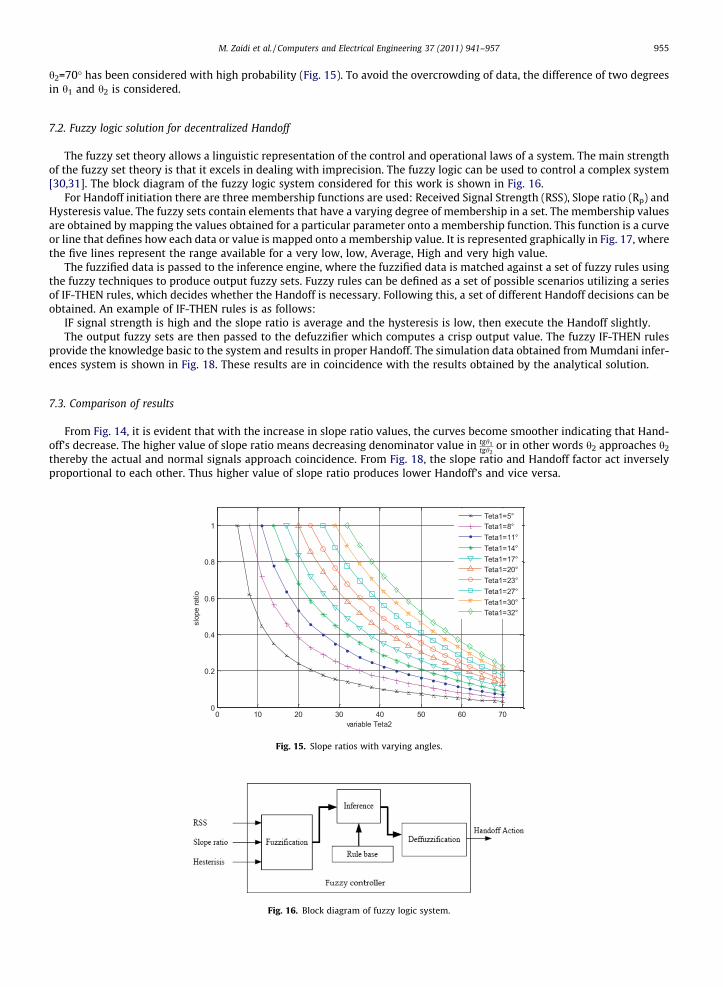
M. Zaidi et al. / Computers and Electrical Engineering 37 (2011) 941–957 955
h2=70� has been considered with high probability (Fig. 15). To avoid the overcrowding of data, the difference of two degreesin h1 and h2 is considered.
7.2. Fuzzy logic solution for decentralized Handoff
The fuzzy set theory allows a linguistic representation of the control and operational laws of a system. The main strengthof the fuzzy set theory is that it excels in dealing with imprecision. The fuzzy logic can be used to control a complex system[30,31]. The block diagram of the fuzzy logic system considered for this work is shown in Fig. 16.
For Handoff initiation there are three membership functions are used: Received Signal Strength (RSS), Slope ratio (Rp) andHysteresis value. The fuzzy sets contain elements that have a varying degree of membership in a set. The membership valuesare obtained by mapping the values obtained for a particular parameter onto a membership function. This function is a curveor line that defines how each data or value is mapped onto a membership value. It is represented graphically in Fig. 17, wherethe five lines represent the range available for a very low, low, Average, High and very high value.
The fuzzified data is passed to the inference engine, where the fuzzified data is matched against a set of fuzzy rules usingthe fuzzy techniques to produce output fuzzy sets. Fuzzy rules can be defined as a set of possible scenarios utilizing a seriesof IF-THEN rules, which decides whether the Handoff is necessary. Following this, a set of different Handoff decisions can beobtained. An example of IF-THEN rules is as follows:
IF signal strength is high and the slope ratio is average and the hysteresis is low, then execute the Handoff slightly.The output fuzzy sets are then passed to the defuzzifier which computes a crisp output value. The fuzzy IF-THEN rules
provide the knowledge basic to the system and results in proper Handoff. The simulation data obtained from Mumdani infer-ences system is shown in Fig. 18. These results are in coincidence with the results obtained by the analytical solution.
7.3. Comparison of results
From Fig. 14, it is evident that with the increase in slope ratio values, the curves become smoother indicating that Hand-off’s decrease. The higher value of slope ratio means decreasing denominator value in tgh1
tgh2or in other words h2 approaches h2
thereby the actual and normal signals approach coincidence. From Fig. 18, the slope ratio and Handoff factor act inverselyproportional to each other. Thus higher value of slope ratio produces lower Handoff’s and vice versa.
0 10 20 30 40 50 60 700
0.2
0.4
0.6
0.8
1
variable Teta2
slop
e ra
tio
Teta1=5°Teta1=8°Teta1=11°Teta1=14°Teta1=17°Teta1=20°Teta1=23°Teta1=27°Teta1=30°Teta1=32°
Fig. 15. Slope ratios with varying angles.
Fig. 16. Block diagram of fuzzy logic system.
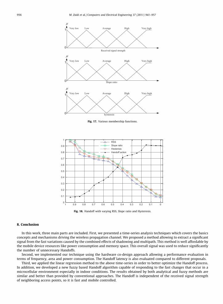
00.10.20.30.40.50.60.70.80.910
0.1
0.2
0.3
0.4
0.5
0.6
0.7
0.8
0.9
1RSSSlope ratioHesterisisHandoff action
Fig. 18. Handoff with varying RSS, Slope ratio and Hysteresis.
1
0Received signal strength
Very low AverageLow High Very high
μ
1
0 Slope ratio
Very low AverageLow High Very high
μ
1
0 hysteresis
Very low AverageLow High Very high
μ
Fig. 17. Various membership functions.
956 M. Zaidi et al. / Computers and Electrical Engineering 37 (2011) 941–957
8. Conclusion
In this work, three main parts are included. First, we presented a time-series analysis techniques which covers the basicsconcepts and mechanisms driving the wireless propagation channel. We proposed a method allowing to extract a significantsignal from the fast variations caused by the combined effects of shadowing and multipath. This method is well affordable bythe mobile device resources like power consumption and memory space. This overall signal was used to reduce significantlythe number of unnecessary Handoffs.
Second, we implemented our technique using the hardware co-design approach allowing a performance evaluation interms of frequency, area and power consumption. The Handoff latency is also evaluated compared to different proposals.
Third, we applied the linear regression method to the above time-series in order to better optimize the Handoff process.In addition, we developed a new fuzzy based Handoff algorithm capable of responding to the fast changes that occur in amicrocellular environment especially in indoor conditions. The results obtained by both analytical and fuzzy methods aresimilar and better than provided by conventional approaches. The Handoff is independent of the received signal strengthof neighboring access points, so it is fast and mobile controlled.
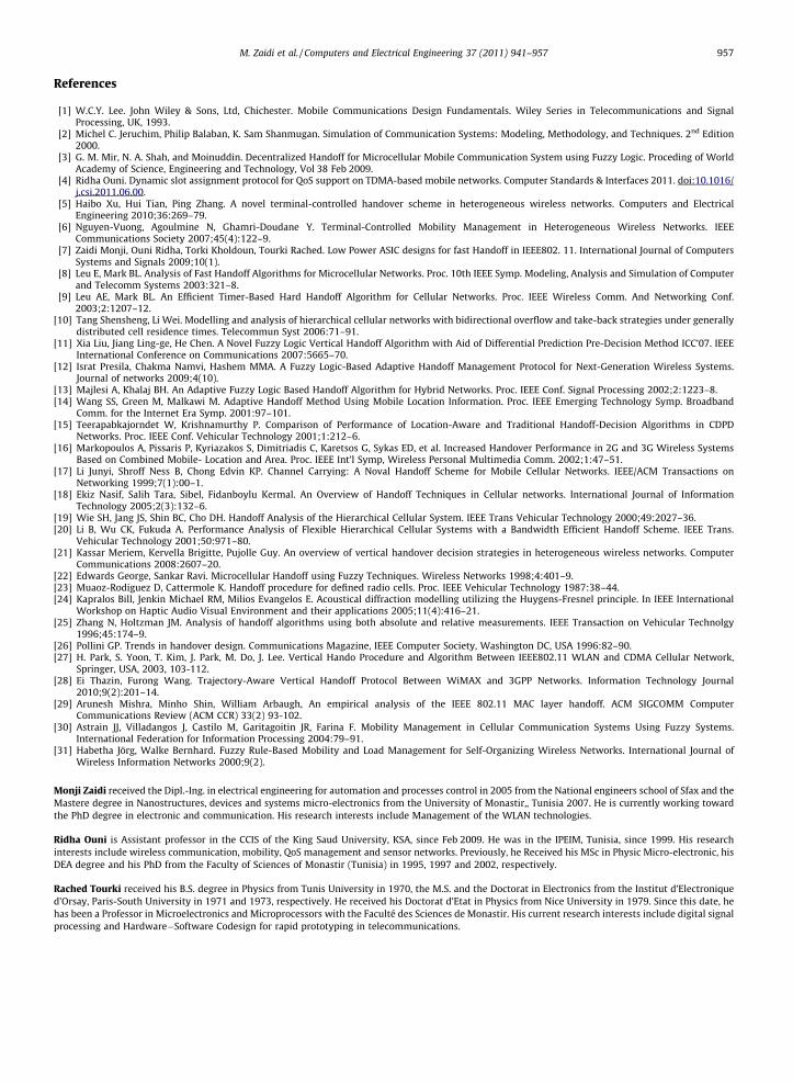
M. Zaidi et al. / Computers and Electrical Engineering 37 (2011) 941–957 957
References
[1] W.C.Y. Lee. John Wiley & Sons, Ltd, Chichester. Mobile Communications Design Fundamentals. Wiley Series in Telecommunications and SignalProcessing, UK, 1993.
[2] Michel C. Jeruchim, Philip Balaban, K. Sam Shanmugan. Simulation of Communication Systems: Modeling, Methodology, and Techniques. 2nd Edition2000.
[3] G. M. Mir, N. A. Shah, and Moinuddin. Decentralized Handoff for Microcellular Mobile Communication System using Fuzzy Logic. Proceding of WorldAcademy of Science, Engineering and Technology, Vol 38 Feb 2009.
[4] Ridha Ouni. Dynamic slot assignment protocol for QoS support on TDMA-based mobile networks. Computer Standards & Interfaces 2011. doi:10.1016/j.csi.2011.06.00.
[5] Haibo Xu, Hui Tian, Ping Zhang. A novel terminal-controlled handover scheme in heterogeneous wireless networks. Computers and ElectricalEngineering 2010;36:269–79.
[6] Nguyen-Vuong, Agoulmine N, Ghamri-Doudane Y. Terminal-Controlled Mobility Management in Heterogeneous Wireless Networks. IEEECommunications Society 2007;45(4):122–9.
[7] Zaidi Monji, Ouni Ridha, Torki Kholdoun, Tourki Rached. Low Power ASIC designs for fast Handoff in IEEE802. 11. International Journal of ComputersSystems and Signals 2009;10(1).
[8] Leu E, Mark BL. Analysis of Fast Handoff Algorithms for Microcellular Networks. Proc. 10th IEEE Symp. Modeling, Analysis and Simulation of Computerand Telecomm Systems 2003:321–8.
[9] Leu AE, Mark BL. An Efficient Timer-Based Hard Handoff Algorithm for Cellular Networks. Proc. IEEE Wireless Comm. And Networking Conf.2003;2:1207–12.
[10] Tang Shensheng, Li Wei. Modelling and analysis of hierarchical cellular networks with bidirectional overflow and take-back strategies under generallydistributed cell residence times. Telecommun Syst 2006:71–91.
[11] Xia Liu, Jiang Ling-ge, He Chen. A Novel Fuzzy Logic Vertical Handoff Algorithm with Aid of Differential Prediction Pre-Decision Method ICC’07. IEEEInternational Conference on Communications 2007:5665–70.
[12] Israt Presila, Chakma Namvi, Hashem MMA. A Fuzzy Logic-Based Adaptive Handoff Management Protocol for Next-Generation Wireless Systems.Journal of networks 2009;4(10).
[13] Majlesi A, Khalaj BH. An Adaptive Fuzzy Logic Based Handoff Algorithm for Hybrid Networks. Proc. IEEE Conf. Signal Processing 2002;2:1223–8.[14] Wang SS, Green M, Malkawi M. Adaptive Handoff Method Using Mobile Location Information. Proc. IEEE Emerging Technology Symp. Broadband
Comm. for the Internet Era Symp. 2001:97–101.[15] Teerapabkajorndet W, Krishnamurthy P. Comparison of Performance of Location-Aware and Traditional Handoff-Decision Algorithms in CDPD
Networks. Proc. IEEE Conf. Vehicular Technology 2001;1:212–6.[16] Markopoulos A, Pissaris P, Kyriazakos S, Dimitriadis C, Karetsos G, Sykas ED, et al. Increased Handover Performance in 2G and 3G Wireless Systems
Based on Combined Mobile- Location and Area. Proc. IEEE Int’l Symp, Wireless Personal Multimedia Comm. 2002;1:47–51.[17] Li Junyi, Shroff Ness B, Chong Edvin KP. Channel Carrying: A Noval Handoff Scheme for Mobile Cellular Networks. IEEE/ACM Transactions on
Networking 1999;7(1):00–1.[18] Ekiz Nasif, Salih Tara, Sibel, Fidanboylu Kermal. An Overview of Handoff Techniques in Cellular networks. International Journal of Information
Technology 2005;2(3):132–6.[19] Wie SH, Jang JS, Shin BC, Cho DH. Handoff Analysis of the Hierarchical Cellular System. IEEE Trans Vehicular Technology 2000;49:2027–36.[20] Li B, Wu CK, Fukuda A. Performance Analysis of Flexible Hierarchical Cellular Systems with a Bandwidth Efficient Handoff Scheme. IEEE Trans.
Vehicular Technology 2001;50:971–80.[21] Kassar Meriem, Kervella Brigitte, Pujolle Guy. An overview of vertical handover decision strategies in heterogeneous wireless networks. Computer
Communications 2008:2607–20.[22] Edwards George, Sankar Ravi. Microcellular Handoff using Fuzzy Techniques. Wireless Networks 1998;4:401–9.[23] Muaoz-Rodiguez D, Cattermole K. Handoff procedure for defined radio cells. Proc. IEEE Vehicular Technology 1987:38–44.[24] Kapralos Bill, Jenkin Michael RM, Milios Evangelos E. Acoustical diffraction modelling utilizing the Huygens-Fresnel principle. In IEEE International
Workshop on Haptic Audio Visual Environment and their applications 2005;11(4):416–21.[25] Zhang N, Holtzman JM. Analysis of handoff algorithms using both absolute and relative measurements. IEEE Transaction on Vehicular Technolgy
1996;45:174–9.[26] Pollini GP. Trends in handover design. Communications Magazine, IEEE Computer Society, Washington DC, USA 1996:82–90.[27] H. Park, S. Yoon, T. Kim, J. Park, M. Do, J. Lee. Vertical Hando Procedure and Algorithm Between IEEE802.11 WLAN and CDMA Cellular Network,
Springer, USA, 2003, 103-112.[28] Ei Thazin, Furong Wang. Trajectory-Aware Vertical Handoff Protocol Between WiMAX and 3GPP Networks. Information Technology Journal
2010;9(2):201–14.[29] Arunesh Mishra, Minho Shin, William Arbaugh, An empirical analysis of the IEEE 802.11 MAC layer handoff. ACM SIGCOMM Computer
Communications Review (ACM CCR) 33(2) 93-102.[30] Astrain JJ, Villadangos J, Castilo M, Garitagoitin JR, Farina F. Mobility Management in Cellular Communication Systems Using Fuzzy Systems.
International Federation for Information Processing 2004:79–91.[31] Habetha Jörg, Walke Bernhard. Fuzzy Rule-Based Mobility and Load Management for Self-Organizing Wireless Networks. International Journal of
Wireless Information Networks 2000;9(2).
Monji Zaidi received the Dipl.-Ing. in electrical engineering for automation and processes control in 2005 from the National engineers school of Sfax and theMastere degree in Nanostructures, devices and systems micro-electronics from the University of Monastir,, Tunisia 2007. He is currently working towardthe PhD degree in electronic and communication. His research interests include Management of the WLAN technologies.
Ridha Ouni is Assistant professor in the CCIS of the King Saud University, KSA, since Feb 2009. He was in the IPEIM, Tunisia, since 1999. His researchinterests include wireless communication, mobility, QoS management and sensor networks. Previously, he Received his MSc in Physic Micro-electronic, hisDEA degree and his PhD from the Faculty of Sciences of Monastir (Tunisia) in 1995, 1997 and 2002, respectively.
Rached Tourki received his B.S. degree in Physics from Tunis University in 1970, the M.S. and the Doctorat in Electronics from the Institut d’Electroniqued’Orsay, Paris-South University in 1971 and 1973, respectively. He received his Doctorat d’Etat in Physics from Nice University in 1979. Since this date, hehas been a Professor in Microelectronics and Microprocessors with the Faculté des Sciences de Monastir. His current research interests include digital signalprocessing and Hardware�Software Codesign for rapid prototyping in telecommunications.
A new energy-efficient neighbor discovery and load balancing protocols for
mobile sensor networks
Ridha Ouni1, Rafik Louati2
1 College of Computer and Information Sciences (CCIS), King Saud University, KSA
2 Ecole Nationale d’Ingénieurs de Monastir (ENIM), Tunisia
Abstract
The wireless sensor networks (WSNs) are formed by a large number of sensor nodes working together to provide a
specific duty. However, the low energy capacity assigned to each node prompts users to look at an important design
challenge which is lifetime maximization. Especially the availability of nodes, the sensor coverage, and the connectivity
have been included in discussions on network lifetime. Therefore, designing effective techniques that conserve scarce
energy resources is a critical issue in WSNs. In this regard, we are interested in developing various mechanisms to save
energy based on the constraints involved in the energy consumption in WSNs. Three mechanisms are proposed to
improve the management of control packets responsible for path discovery, self-organization, and balance the load
distribution in the network.
Keywords: Wireless Sensor Networks, lifetime, AODV Routing, Energy-aware routing
1. Introduction
With the proliferation of wireless sensor networks
(WSN), completely new application domains for
wireless ad hoc networks have emerged. These later
motivated an increasing demand for developing more
efficient sensor networks despite their limitations in the
available resources (energy, processing speed, storage).
Besides these restrictions, WSNs are also exposed to
various requirements dealing with dynamic topologies
and variable environmental conditions [1]. Moreover,
routing and data dissemination constraints [2], self-
organization issues [3] and the efficient deployment of
sensor nodes [4] have already been investigated. While
the study of network lifetime as a key characteristic of
WSNs is still in progress [5].
Energy is a critical factor in wireless sensor
networks (WSN). To increase the network lifetime, the
energy must be conserved in hardware as well as in
software that comprise the network architecture. The
data communication is the most responsible factor in the
consumption of energy budget in comparison with
sensing and computing [6]. Therefore, it is desirable to
use short-range nodes instead of long range due to the
power required in transmission. In most scenarios, the
events can be detected by several nodes close to the
source of the phenomenon. Then, using short-range
communication leads necessarily to a multi-hop data
packets transmission.
Consumption optimization is a crucial issue in WSNs
that requires optimizing radio communication
processing and traffic load. This includes digital
devices, a microcontroller, application software and the
various algorithms for energy management.
A great number of algorithms and methods were
proposed to increase the lifetime of a sensor network by
reducing energy consumption according to their
application types, constraints, and network architecture.
Some previous works discuss reliable multipath routing
with energy efficiency [7] and exploiting latency and
density [8]. Other works reduce radio activities as key
management protocols [9] and multiple base stations
[10].
In this paper, we are interested to propose an
Enhanced model of the Ad Hoc On Demand Distance
Vector (EAODV) protocol. EAODV is designed to
reduce the number of control packets, create an historic
routing data base and balance the network load which
result decreasing the energy consumption. Then, we
discuss a comparative study of capabilities offered by
both of AODV and EAODV protocol. Several metrics
are undertaken to evaluate performances of EAODV
protocol.
This paper is organized as follows. Section 2
summarizes the related works. Section 3 introduces the
concept of EAODV protocol and its mechanisms to
decrease energy consumption. Section 4 outlines the
simulation results evaluating the performances of
EAODV protocol compared to AODV. Finally,
section 5 concludes the paper.
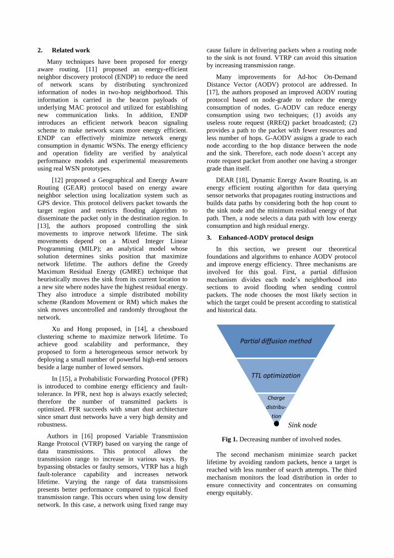
2. Related work
Many techniques have been proposed for energy
aware routing. [11] proposed an energy-efficient
neighbor discovery protocol (ENDP) to reduce the need
of network scans by distributing synchronized
information of nodes in two-hop neighborhood. This
information is carried in the beacon payloads of
underlying MAC protocol and utilized for establishing
new communication links. In addition, ENDP
introduces an efficient network beacon signaling
scheme to make network scans more energy efficient.
ENDP can effectively minimize network energy
consumption in dynamic WSNs. The energy efficiency
and operation fidelity are verified by analytical
performance models and experimental measurements
using real WSN prototypes.
[12] proposed a Geographical and Energy Aware
Routing (GEAR) protocol based on energy aware
neighbor selection using localization system such as
GPS device. This protocol delivers packet towards the
target region and restricts flooding algorithm to
disseminate the packet only in the destination region. In
[13], the authors proposed controlling the sink
movements to improve network lifetime. The sink
movements depend on a Mixed Integer Linear
Programming (MILP); an analytical model whose
solution determines sinks position that maximize
network lifetime. The authors define the Greedy
Maximum Residual Energy (GMRE) technique that
heuristically moves the sink from its current location to
a new site where nodes have the highest residual energy.
They also introduce a simple distributed mobility
scheme (Random Movement or RM) which makes the
sink moves uncontrolled and randomly throughout the
network.
Xu and Hong proposed, in [14], a chessboard
clustering scheme to maximize network lifetime. To
achieve good scalability and performance, they
proposed to form a heterogeneous sensor network by
deploying a small number of powerful high-end sensors
beside a large number of lowed sensors.
In [15], a Probabilistic Forwarding Protocol (PFR)
is introduced to combine energy efficiency and fault-
tolerance. In PFR, next hop is always exactly selected;
therefore the number of transmitted packets is
optimized. PFR succeeds with smart dust architecture
since smart dust networks have a very high density and
robustness.
Authors in [16] proposed Variable Transmission
Range Protocol (VTRP) based on varying the range of
data transmissions. This protocol allows the
transmission range to increase in various ways. By
bypassing obstacles or faulty sensors, VTRP has a high
fault-tolerance capability and increases network
lifetime. Varying the range of data transmissions
presents better performance compared to typical fixed
transmission range. This occurs when using low density
network. In this case, a network using fixed range may
cause failure in delivering packets when a routing node
to the sink is not found. VTRP can avoid this situation
by increasing transmission range.
Many improvements for Ad-hoc On-Demand
Distance Vector (AODV) protocol are addressed. In
[17], the authors proposed an improved AODV routing
protocol based on node-grade to reduce the energy
consumption of nodes. G-AODV can reduce energy
consumption using two techniques; (1) avoids any
useless route request (RREQ) packet broadcasted; (2)
provides a path to the packet with fewer resources and
less number of hops. G-AODV assigns a grade to each
node according to the hop distance between the node
and the sink. Therefore, each node doesn’t accept any
route request packet from another one having a stronger
grade than itself.
DEAR [18], Dynamic Energy Aware Routing, is an
energy efficient routing algorithm for data querying
sensor networks that propagates routing instructions and
builds data paths by considering both the hop count to
the sink node and the minimum residual energy of that
path. Then, a node selects a data path with low energy
consumption and high residual energy.
3. Enhanced-AODV protocol design
In this section, we present our theoretical
foundations and algorithms to enhance AODV protocol
and improve energy efficiency. Three mechanisms are
involved for this goal. First, a partial diffusion
mechanism divides each node’s neighborhood into
sections to avoid flooding when sending control
packets. The node chooses the most likely section in
which the target could be present according to statistical
and historical data.
Fig 1. Decreasing number of involved nodes.
The second mechanism minimize search packet
lifetime by avoiding random packets, hence a target is
reached with less number of search attempts. The third
mechanism monitors the load distribution in order to
ensure connectivity and concentrates on consuming
energy equitably.
Partial diffusion method
TTL optimization
Charge
distribu-
tion
Sink node
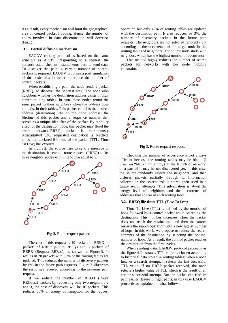
As a result, every mechanism will limit the geographical
area of control packet flooding. Hence, the number of
nodes involved in data dissemination will decrease
(Fig.1).
3.1. Partial diffusion mechanism
EAODV routing protocol is based on the same
principle as AODV. Responding to a request, the
network establishes an instantaneous path to send data.
To discover the path, a certain number of control
packets is required. EAODV proposes a post simulation
of the basic idea in order to reduce the number of
control packets.
When establishing a path, the node sends a packet
(RREQ) to discover the shortest way. The node asks
neighbors whether the destination address exists in their
current routing tables. In turn, these nodes return the
same packet to their neighbors when the address does
not exist in their tables. This packet contains the desired
address (destination), the source node address, the
lifetime of this packet and a sequence number that
serves as a unique identifier of the packet. By mobility
effect of the destination node, this packet may flood the
entire network. RREQ packet is continuously
retransmitted until requested destination is reached,
unless the declared life time of the packet (TTL: Time
To Live) has expired.
In Figure 2, the source tries to send a message to
the destination. It sends a route request (RREQ) to its
three neighbor nodes with time to live equal to 5.
Fig 2. Route request packet.
The cost of this request is 10 packets of RREQ, 4
packets of RREP (Route REPly) and 6 packets of
RERR (Request ERRor), as shown in Figure 3. It
results in 20 packets with 85% of the routing tables are
updated. This reduces the number of discovery packets
by 6% in the future path requests. Figure 3 illustrates
the responses received according to the previous path
request.
If we reduce the number of RREQ (Route
REQuest) packets by requesting only two neighbors 2
and 3, the cost of discovery will be 10 packets. This
reduces 50% of energy consumption for the request
operation but only 45% of routing tables are updated
with the destination path. It also reduces, by 3%, the
number of discovery packets in the future path
requests. The neighbors are not selected randomly but
according to the occurrence of the target node in the
routing tables of neighbors. The source node starts with
neighbors which has the highest number of occurrence.
This method highly reduces the number of search
packets for networks with low node mobility
constraint.
Fig 3. Route request response.
Checking the number of occurrence is not always
efficient because the routing tables may be blank {I
insist on “blank” not empty} at the launch of network,
or a part of it may be not discovered yet. In this case,
the source randomly selects the neighbors, and then
diffuses packets partially through it. Information
collected in the search task is stored then used in a
future search attempts. This information is about the
energy level of neighbors and the occurrence of
addresses that appear in each routing table.
3.2. RREQ life time: TTL (Time To Live)
Time To Live (TTL) is defined by the number of
hops followed by a control packet while searching the
destination. This number increases when the packet
does not reach the destination, and then the source
restarts the search operation with a new higher number
of hops. In this work, we propose to reduce the search
attempts of the destination by selecting the optimal
number of hops. As a result, the control packet reaches
the destination from the first cycles.
When sending data, EAODV protocol proceeds as
the figure 4 illustrates. TTL value is chosen according
to historical data stored in routing tables; when a node
lunches a search attempt, it selects the last successful
TTL value. If no RREP packet received, the node
selects a higher value of TLL which is the result of an
earlier successful attempt. But the packet can find its
path earlier (figure 5, right path); in this case EAODV
proceeds as explained in what follows.
RREP
RREP
RREP
RREP
RERR
RERR
RERR
RERR
RERR
RERR
RERR
1
2
3
RREQ
RREQ
RREQ
RREQ
RREQ
RREQ
RREQ
RREQ
RREQ
RREQ
RREQ
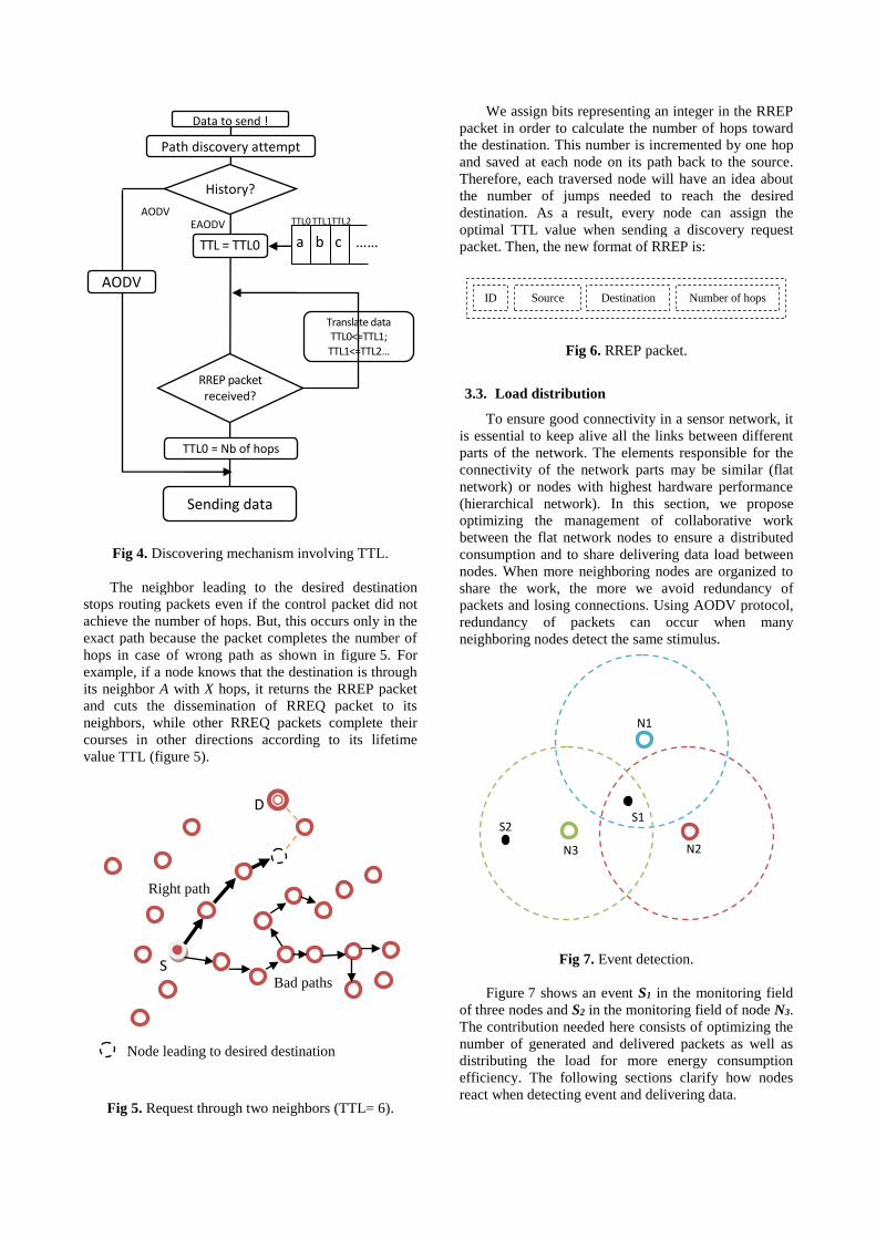
Fig 4. Discovering mechanism involving TTL.
The neighbor leading to the desired destination
stops routing packets even if the control packet did not
achieve the number of hops. But, this occurs only in the
exact path because the packet completes the number of
hops in case of wrong path as shown in figure 5. For
example, if a node knows that the destination is through
its neighbor A with X hops, it returns the RREP packet
and cuts the dissemination of RREQ packet to its
neighbors, while other RREQ packets complete their
courses in other directions according to its lifetime
value TTL (figure 5).
Fig 5. Request through two neighbors (TTL= 6).
We assign bits representing an integer in the RREP
packet in order to calculate the number of hops toward
the destination. This number is incremented by one hop
and saved at each node on its path back to the source.
Therefore, each traversed node will have an idea about
the number of jumps needed to reach the desired
destination. As a result, every node can assign the
optimal TTL value when sending a discovery request
packet. Then, the new format of RREP is:
Fig 6. RREP packet.
3.3. Load distribution
To ensure good connectivity in a sensor network, it
is essential to keep alive all the links between different
parts of the network. The elements responsible for the
connectivity of the network parts may be similar (flat
network) or nodes with highest hardware performance
(hierarchical network). In this section, we propose
optimizing the management of collaborative work
between the flat network nodes to ensure a distributed
consumption and to share delivering data load between
nodes. When more neighboring nodes are organized to
share the work, the more we avoid redundancy of
packets and losing connections. Using AODV protocol,
redundancy of packets can occur when many
neighboring nodes detect the same stimulus.
Fig 7. Event detection.
Figure 7 shows an event S1 in the monitoring field
of three nodes and S2 in the monitoring field of node N3.
The contribution needed here consists of optimizing the
number of generated and delivered packets as well as
distributing the load for more energy consumption
efficiency. The following sections clarify how nodes
react when detecting event and delivering data.
S2 S1
N1
N2 N3
ID Source Destination Number of hops
Right path
Bad paths S
D
Node leading to desired destination
Translate data TTL0<=TTL1; TTL1<=TTL2…
Data to send !
Path discovery attempt
History?
TTL = TTL0
RREP packet received?
……
TTL0 = Nb of hops
b c
TTL0 TTL1 TTL2
AODVproc
Sending data
EAODV AODV
a
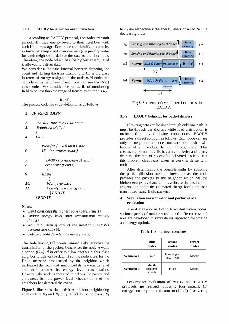
3.3.1. EAODV behavior for event detection
According to EAODV protocol, the nodes transmit
periodically their energy levels to their neighbors with
each Hello message. Each node can classify its capacity
in terms of energy and then can assign a priority order
for each neighbor to deliver the data to the sink node.
Therefore, the node which has the highest energy level
is allowed to deliver data.
We consider ti the time interval between detecting the
event and starting the transmission, and Cn is the class
in terms of energy assigned to the node n. N nodes are
considered as neighbors if each one can see the (N-1)
other nodes. We consider the radius RS of monitoring
field to be less than the range of transmission radius RP.
RS < RP
The process code for event detection is as follows:
1. IF (Cn=1) THEN {
2. EAODV transmission attempt 3. Broadcast (Hello !)
} 4. ELSE
{ 5. Wait (ti* (Cn-1)) AND Listen 6. IF (no transmissions)
{ 7. EAODV transmission attempt 8. broadcast (Hello !)
} 9. ELSE
{ 10. Wait for(Hello !) 11. Classify new energy data
} END IF
} END IF
Notes.
Cn=1 considers the highest power level (line 1).
Update energy level after transmission activity
(line 3).
Wait and listen if any of the neighbors initiates
transmission (line 5).
Only one node detected the event (line 7).
The node having full power, immediately launches the
transmission of the packet. Otherwise, the node n waits
a period (Cn-1)×ti in order to allow another higher class
neighbor to deliver the data. If so, the node waits for the
Hello message broadcasted by the neighbor which
performed the work and announced its new energy level
and then updates its energy level classification.
However, the node is required to deliver the packet and
announces its new power level whether none of the
neighbors has detected the event.
Figure 8 illustrates the activities of four neighboring
nodes where N3 and N4 only detect the same event. E1
to E4 are respectively the energy levels of N1 to N4 in a
decreasing order.
Fig 8. Sequence of event detection process in
EAODV.
3.3.2. EAODV behavior for packet delivery
If routing data can be done through only one path, it
must be through the shortest while load distribution is
maintained to avoid losing connections. EAODV
provides a direct solution as follows. Each node can see
only its neighbors and does not care about what will
happen after providing the data through them. This
creates a problem if traffic has a high priority and it may
decrease the rate of successful delivered packets. But
this problem disappears when network is dense with
nodes.
After determining the possible paths by adopting
the partial diffusion method shown above, the node
provides the packets to the neighbor which has the
highest energy level and admits a link to the destination.
Information about the estimated charge levels are then
transmitted using Hello packets.
4. Simulation environment and performance
evaluation
Several scenarios including fixed destination nodes,
various speeds of mobile sensors and different covered
area are developed to simulate our approach for routing
and energy optimization.
Table 1. Simulation scenarios.
sink
nodes
sensor
nodes
target
nodes
Scenario 1 Fixed 8 moving at low speed
Mobile
Scenario 2 Mobile
different speeds
Fixed Mobile
Performance evaluation of AODV and EAODV
protocols are realized following four aspects: (1)
energy consumption estimator model (2) discovering
N1
N2
N3
N4
E1
Sensing and listening to channel
Event Wait & listen
Sensing and listening to channel
Event Detection
Wait & listen
Listen
Hello!
Data
receiving
Transmitting
Data receiving
Data receiving
E2
E3
E4
2 T
3T
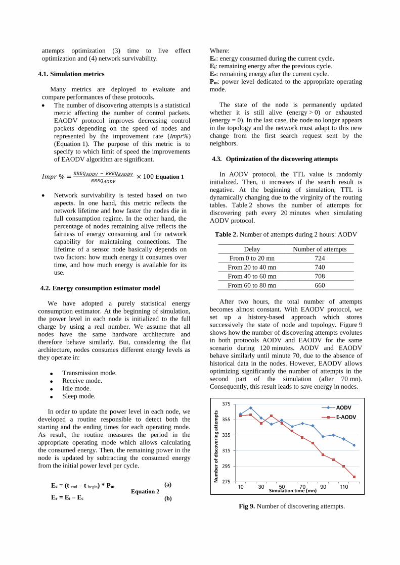
attempts optimization (3) time to live effect
optimization and (4) network survivability.
4.1. Simulation metrics
Many metrics are deployed to evaluate and
compare performances of these protocols.
The number of discovering attempts is a statistical
metric affecting the number of control packets.
EAODV protocol improves decreasing control
packets depending on the speed of nodes and
represented by the improvement rate (Impr%)
(Equation 1). The purpose of this metric is to
specify to which limit of speed the improvements
of EAODV algorithm are significant.
𝐼𝑚𝑝𝑟 % =𝑅𝑅𝐸𝑄𝐴𝑂𝐷𝑉 − 𝑅𝑅𝐸𝑄𝐸𝐴𝑂𝐷𝑉
𝑅𝑅𝐸𝑄𝐴𝑂𝐷𝑉 × 100 Equation 1
Network survivability is tested based on two
aspects. In one hand, this metric reflects the
network lifetime and how faster the nodes die in
full consumption regime. In the other hand, the
percentage of nodes remaining alive reflects the
fairness of energy consuming and the network
capability for maintaining connections. The
lifetime of a sensor node basically depends on
two factors: how much energy it consumes over
time, and how much energy is available for its
use.
4.2. Energy consumption estimator model
We have adopted a purely statistical energy
consumption estimator. At the beginning of simulation,
the power level in each node is initialized to the full
charge by using a real number. We assume that all
nodes have the same hardware architecture and
therefore behave similarly. But, considering the flat
architecture, nodes consumes different energy levels as
they operate in:
Transmission mode.
Receive mode.
Idle mode.
Sleep mode.
In order to update the power level in each node, we
developed a routine responsible to detect both the
starting and the ending times for each operating mode.
As result, the routine measures the period in the
appropriate operating mode which allows calculating
the consumed energy. Then, the remaining power in the
node is updated by subtracting the consumed energy
from the initial power level per cycle.
Ec = (t end – t begin) * Pm
Er = Ei – Ec
(a)
Equation 2
(b)
Where:
Ec: energy consumed during the current cycle.
Ei: remaining energy after the previous cycle.
Er: remaining energy after the current cycle.
Pm: power level dedicated to the appropriate operating
mode.
The state of the node is permanently updated
whether it is still alive (energy > 0) or exhausted
(energy = 0). In the last case, the node no longer appears
in the topology and the network must adapt to this new
change from the first search request sent by the
neighbors.
4.3. Optimization of the discovering attempts
In AODV protocol, the TTL value is randomly
initialized. Then, it increases if the search result is
negative. At the beginning of simulation, TTL is
dynamically changing due to the virginity of the routing
tables. Table 2 shows the number of attempts for
discovering path every 20 minutes when simulating
AODV protocol.
Table 2. Number of attempts during 2 hours: AODV
Delay Number of attempts
From 0 to 20 mn 724
From 20 to 40 mn 740
From 40 to 60 mn 708
From 60 to 80 mn 660
After two hours, the total number of attempts
becomes almost constant. With EAODV protocol, we
set up a history-based approach which stores
successively the state of node and topology. Figure 9
shows how the number of discovering attempts evolutes
in both protocols AODV and EAODV for the same
scenario during 120 minutes. AODV and EAODV
behave similarly until minute 70, due to the absence of
historical data in the nodes. However, EAODV allows
optimizing significantly the number of attempts in the
second part of the simulation (after 70 mn).
Consequently, this result leads to save energy in nodes.
Fig 9. Number of discovering attempts.
275
295
315
335
355
375
10 30 50 70 90 110
Nu
mb
er
of
dis
cove
rin
g at
tem
pts
Simulation time (mn)
AODV
E-AODV
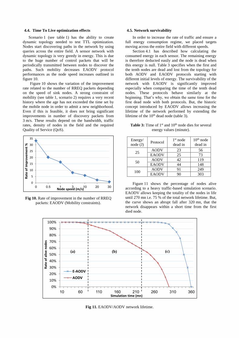
4.4. Time To Live optimization effects
Scenario 1 (see table 1) has the ability to create
dynamic topology needed to test TTL optimization.
Nodes start discovering paths in the network by using
queries across the entire field. A sensor network with
dynamic topology is very greedy in energy. This is due
to the huge number of control packets that will be
periodically transmitted between nodes to discover the
paths. Such mobility decreases EAODV protocol
performances as the node speed increases outlined in
figure 10.
Figure 10 shows the variation of the improvement
rate related to the number of RREQ packets depending
on the speed of sink nodes. A strong constraint of
mobility (see table 1, scenario 2) requires a very recent
history where the age has not exceeded the time set by
the mobile node in order to admit a new neighborhood.
Even if this is feasible, it does not bring significant
improvements in number of discovery packets from
3 m/s. These results depend on the bandwidth, traffic
rates, density of nodes in the field and the required
Quality of Service (QoS).
Fig 10. Rate of improvement in the number of RREQ
packets: EAODV (Mobility constraints).
4.5. Network survivability
In order to increase the rate of traffic and ensure a
full energy consumption regime, we placed targets
moving across the entire field with different speeds.
Section 4.1 has described how calculating the
consumed energy in each sensor. The remaining energy
is therefore deducted easily and the node is dead when
this energy is null. Table 3 specifies when the first and
the tenth nodes are dead and lost from the topology for
both AODV and EAODV protocols starting with
different initial levels of energy. The survivability of the
network with EAODV is significantly improved
especially when comparing the time of the tenth dead
nodes. These protocols behave similarly at the
beginning. That’s why, we obtain the same time for the
first dead node with both protocols. But, the historic
concept introduced by EAODV allows increasing the
lifetime of the network performed by extending the
lifetime of the 10th dead node (table 3).
Table 3: Time of 1st and 10th node dies for several
energy values (minute).
Energy/
node (J) Protocol
1st node
dead in
10th node
dead in
25 AODV 23 56
EAODV 25 73
50 AODV 42 119
EAODV 44 148
100 AODV 91 249
EAODV 90 303
Figure 11 shows the percentage of nodes alive
according to a heavy traffic-based simulation scenario.
EAODV allows keeping the totality of the nodes in life
until 270 mn i.e. 75 % of the total network lifetime. But,
the curve shows an abrupt fall after 320 mn, that the
network disappears within a short time from the first
died node.
Fig 11. EAODV/AODV network lifetime.
0
5
10
15
20
25
30
35
0 0.5 1 3 10 20 30
Rat
e o
f im
pro
vem
en
t %
Node speed (m/s)
0%
10%
20%
30%
40%
50%
60%
70%
80%
90%
100%
10 60 110 160 210 260 310 360
Rat
e o
f al
ive
no
de
s
Simulation time (mn)
E-AODV
AODV
(a) (b) (c)
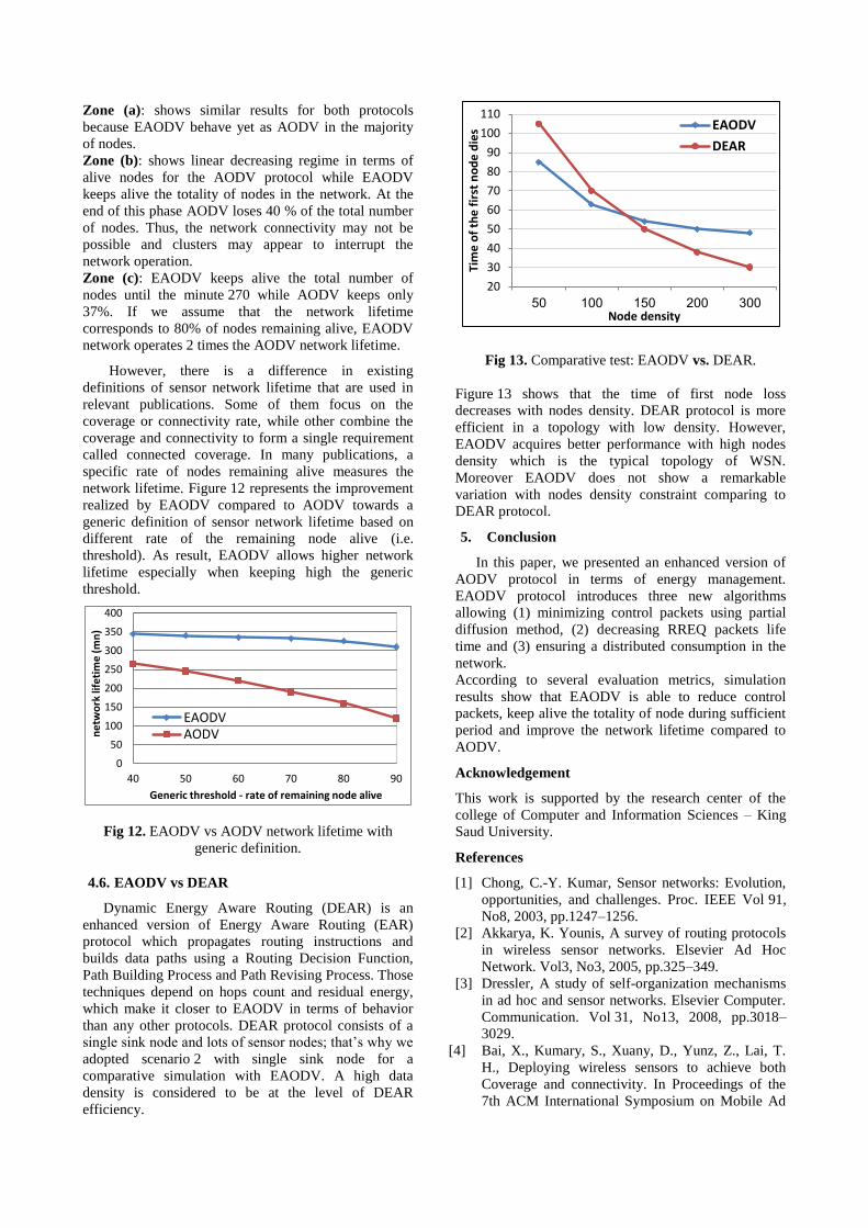
Zone (a): shows similar results for both protocols
because EAODV behave yet as AODV in the majority
of nodes.
Zone (b): shows linear decreasing regime in terms of
alive nodes for the AODV protocol while EAODV
keeps alive the totality of nodes in the network. At the
end of this phase AODV loses 40 % of the total number
of nodes. Thus, the network connectivity may not be
possible and clusters may appear to interrupt the
network operation.
Zone (c): EAODV keeps alive the total number of
nodes until the minute 270 while AODV keeps only
37%. If we assume that the network lifetime
corresponds to 80% of nodes remaining alive, EAODV
network operates 2 times the AODV network lifetime.
However, there is a difference in existing
definitions of sensor network lifetime that are used in
relevant publications. Some of them focus on the
coverage or connectivity rate, while other combine the
coverage and connectivity to form a single requirement
called connected coverage. In many publications, a
specific rate of nodes remaining alive measures the
network lifetime. Figure 12 represents the improvement
realized by EAODV compared to AODV towards a
generic definition of sensor network lifetime based on
different rate of the remaining node alive (i.e.
threshold). As result, EAODV allows higher network
lifetime especially when keeping high the generic
threshold.
Fig 12. EAODV vs AODV network lifetime with
generic definition.
4.6. EAODV vs DEAR
Dynamic Energy Aware Routing (DEAR) is an
enhanced version of Energy Aware Routing (EAR)
protocol which propagates routing instructions and
builds data paths using a Routing Decision Function,
Path Building Process and Path Revising Process. Those
techniques depend on hops count and residual energy,
which make it closer to EAODV in terms of behavior
than any other protocols. DEAR protocol consists of a
single sink node and lots of sensor nodes; that’s why we
adopted scenario 2 with single sink node for a
comparative simulation with EAODV. A high data
density is considered to be at the level of DEAR
efficiency.
Fig 13. Comparative test: EAODV vs. DEAR.
Figure 13 shows that the time of first node loss
decreases with nodes density. DEAR protocol is more
efficient in a topology with low density. However,
EAODV acquires better performance with high nodes
density which is the typical topology of WSN.
Moreover EAODV does not show a remarkable
variation with nodes density constraint comparing to
DEAR protocol.
5. Conclusion
In this paper, we presented an enhanced version of
AODV protocol in terms of energy management.
EAODV protocol introduces three new algorithms
allowing (1) minimizing control packets using partial
diffusion method, (2) decreasing RREQ packets life
time and (3) ensuring a distributed consumption in the
network.
According to several evaluation metrics, simulation
results show that EAODV is able to reduce control
packets, keep alive the totality of node during sufficient
period and improve the network lifetime compared to
AODV.
Acknowledgement
This work is supported by the research center of the
college of Computer and Information Sciences – King
Saud University.
References
[1] Chong, C.-Y. Kumar, Sensor networks: Evolution,
opportunities, and challenges. Proc. IEEE Vol 91,
No8, 2003, pp.1247–1256.
[2] Akkarya, K. Younis, A survey of routing protocols
in wireless sensor networks. Elsevier Ad Hoc
Network. Vol3, No3, 2005, pp.325–349.
[3] Dressler, A study of self-organization mechanisms
in ad hoc and sensor networks. Elsevier Computer.
Communication. Vol 31, No13, 2008, pp.3018–
3029.
[4] Bai, X., Kumary, S., Xuany, D., Yunz, Z., Lai, T.
H., Deploying wireless sensors to achieve both
Coverage and connectivity. In Proceedings of the
7th ACM International Symposium on Mobile Ad
0
50
100
150
200
250
300
350
400
40 50 60 70 80 90
ne
two
rk li
feti
me
(m
n)
Generic threshold - rate of remaining node alive
EAODVAODV
20
30
40
50
60
70
80
90
100
110
50 100 150 200 300
Tim
e o
f th
e f
irst
no
de
die
s
Node density
EAODV
DEAR
Hoc Networking and Computing (ACM Mobihoc),
2006, pp.131–142.
[5] Dietrich, I. and Dressler, On the lifetime of wireless
sensor networks. ACM Transaction on Sensor
Networks. Vol 5, No.1, 2009, 39 pages. [6] J. Hill, et al. System Architecture Directions for
Network Sensors, Proc. of the 9th International
Conference on Architectural Support for
Programming Languages and Operating Systems,
pp. 93–104, Nov. 2000.
[7] U.B. Mahadevaswamy, M.N. Shanmukhaswamy,
An Energy Efficient Reliable Multipath Routing
Protocol for Data Gathering In Wireless Sensor
Networks, (IJCSIS) International Journal of
Computer Science and Information Security, Vol.
8, No. 2, May 2010.
[8] C. Schurgers, V. Tsiatsis, S. Ganeriwal, and M.
Srivastava. Topology management for sensor
networks: Exploiting latency and density. In
Proceedings of MOBICOM, 2002.
[9] Sungha Pete Kim Bo-Cheng Charles Lai, David D.
Hwang. Reducing radio energy consumption of
key management protocols for wireless sensor
networks. ACM 1-58113-929-2/04/0008, pp. 9-11,
August 2004.
[10] Rao, S., Gandham, S., Dawande, M., Prakash, R.,
and Venkatesan, S. (2003). Energy efficient
schemes for wireless sensor networks with
multiple mobile base stations. In Proc. IEEE
Globecom, volume 22, pp. 377–381, San
Francisco, USA.
[11] Mikko Kohvakka , Jukka Suhonen, Mauri
Kuorilehto, Ville Kaseva, H. Marko, Timo D.
Energy-efficient neighbor discovery protocol for
mobile wireless sensor networks, ACM/Elsevier
Ad hoc Networks, 2007.
[12] R. G. Yan Yu and D. Estrin. Geographical and
energy aware routing: a recursive data
dissemination protocol for wireless sensor
networks, May 2002.
[13] S. Basagni, A. Carosi, E. Melachrinoudis, C.
Petrioli, and M. Z.Wang. Controlled sink mobility
for prolonging wireless sensor networks lifetime.
ACM/Elsevier Wireless Networks, 2008.
[14] X. Du, and Y. Xiao. Energy efficient chessboard
clustering and routing in heterogeneous sensor
networks. International Journal of Wireless and
Mobile Computing, 121–130, 2006.
[15] I.Chatzigiannakis, T. Dimitriou, S. Nikoletseas,
and P. Spirakis. A probabilistic algorithm for
efficient and robust data propagation in smart dust
networks. In Proceedings of the 5th European
Wireless Conference on Mobile and Wireless
Systems Beyond 3G (EW 2004), 2004.
[16] T. Antoniou, A. Boukerche, I. Chatzigiannakis, G.
Mylonas, and S. Nikoletseas. A new energy
efficient and fault-tolerant protocol for data
propagation in smart dust networks using varying
transmission range. In Proceedings of the 37th
Annual ACM/IEEE Simulation Symposium
(ANSS ’04), 2004.
[17] Fei Tong Wan Tang Li-Mei Peng Rong Xie
Won-Hyuk Yang Young-Chon Kim. A Node-
Grade Based AODV Routing Protocol for
Wireless Sensor Network. In Proceeding of the
Second IEEE International Conference on
Networks Security Wireless Communications and
Trusted Computing (NSWCTC), 2010, pp. 180–
183, 2010.
[18] Li-Min Sun, Ting-Xin Yan, Yan-Zhong Bi, and
Hong-Song Zhu. A Self-adaptive Energy-Aware
Data Gathering Mechanism for Wireless Sensor
Networks. ICIC 2005, Part II, LNCS 3645,
pp. 588 – 597, Springer 2005.
Papiers publiés dans des
JOURNAUX INTERNATIONAUX
1. Ridha OUNI, Graph splitting based self-organization approach for energy and routing optimization,
International Journal of Digital Information and Wireless Communications (IJDIWC) 1(3): pp 738-
744, 2012.
2. Jamila BHAR, Ridha OUNI, Monji ZAIDI, Salem NASRI, A new TDMA-CR model for dynamic
resource allocation in wireless networks, IJCSES International Journal of Computer Sciences and
Engineering Systems, Vol.4, No.1, January 2010.
3. Monji ZAIDI, Ridha OUNI, Jamila BHAR, Rached TOURKI, New approaches reducing handoff
latency in 802.11 wireless LANs, IJCSES International Journal of Computer Sciences and Engineering
Systems, Vol.3, No.3, July 2009.
4. Monji Zaidi, Ridha OUNI, Kholdoun Torki and Rached Tourki, Low power ASIC designs for fast
Handoff in IEEE802.11, International Journal of Computers, Systems and Signals, Vol. 10, No.1,
pp 27-39, 2009.
5. Jamila BHAR, Ridha OUNI, Abdelhamid HELALI, Salem NASRI, Evaluation of Handover protocols
in Wireless ATM networks, Information Technology Journal (Asian Network for Scientific
Information), Vol 6, N°2, pp 275-282, 2007.
6. Jamila BHAR, Ridha OUNI, Kholdoun TORKI, Salem NASRI, Handovers strategies challenges in
wireless ATM networks, International Journal of Applied Mathematics and Computer Sciences, Vol 4,
N°2, pp 636-641, April 2007.
International Journal of Digital Information and Wireless Communications (IJDIWC) 1(3): 738-744
The Society of Digital Information and Wireless Communications, 2012(ISSN 2225-658X)
738
Graph splitting based self-organization approach for energy and routing optimization
Ridha OUNI
College of Computer and Information Sciences, King Saud University, KSA.
ABSTRACT
Recent advances in wireless sensor networks
have led to many new protocols specifically
designed for sensor networks where energy
awareness is an essential consideration. Both
self-organization and routing protocols
significantly impact the energy consumption
and therefore the network life time. This
paper surveys recent self-organization and
routing protocols for sensor networks and
proposes enhanced approaches for low duty
cycle and more reliable environment. We
compare some of the relays-based protocols
in a random graph model. Simulation results
will show the impact of a graph splitting
approach on the active node set and the
topology connectivity. Moreover, we analyze
the performance of that approach in terms of
transmitted and received packet rate.
KEYWORDS
WSN, MPR, MPR-CDS, Graph split.
1. INTRODUCTION
Smart environments represent the next
evolutionary development step in building,
utilities, industrial, home and transportation
systems automation. The information needed
by smart environments is provided by
Distributed Wireless Sensor Networks
(WSN), which are responsible for sensing as
well as for the first stages of the processing
hierarchy. The individual devices in a WSN
are inherently resource constrained: They
have limited processing speed, storage
capacity, and communication bandwidth.
These devices have substantial processing
capability in the aggregate, but not
individually, so they must organize
themselves and provide a means of
programming and managing the network as
an ensemble, rather than administering
individual devices.
Energy conservation is one of the most
challenging problems because batteries have
very limited capacities. Two particular
important problems are activity scheduling
and broadcasting. In activity scheduling
problem, some nodes decide to sleep to
preserve the energy, but should have an active
neighbor to collect messages for them or take
over some sensing tasks. In broadcasting
problem, one host needs to send a particular
message to all the other ones in the network.
Broadcasting is applied for publication of
services, alarming and other operations. In a
straightforward solution to broadcasting,
hosts only need to blindly relay packets at
least once to their neighborhood. However,
this leads to the well-known broadcast storm
problem as redundancy and collisions [1,2].
Self-organization protocols are proposed in
literature trying to avoid these problems by
choosing active and connected nodes set
charged of broadcasting and routing [3,4,5,6].
The concept of multipoint relaying [7,8]
consists to reduce the number of duplicated
re-transmissions when forwarding a broadcast
packet. This technique restricts the number of
re-transmitters to a small set of neighbor
nodes, instead of all neighbors, like in pure
flooding. This set is kept small as much as
possible by efficiently selecting the neighbors
which covers (in terms of one-hop radio
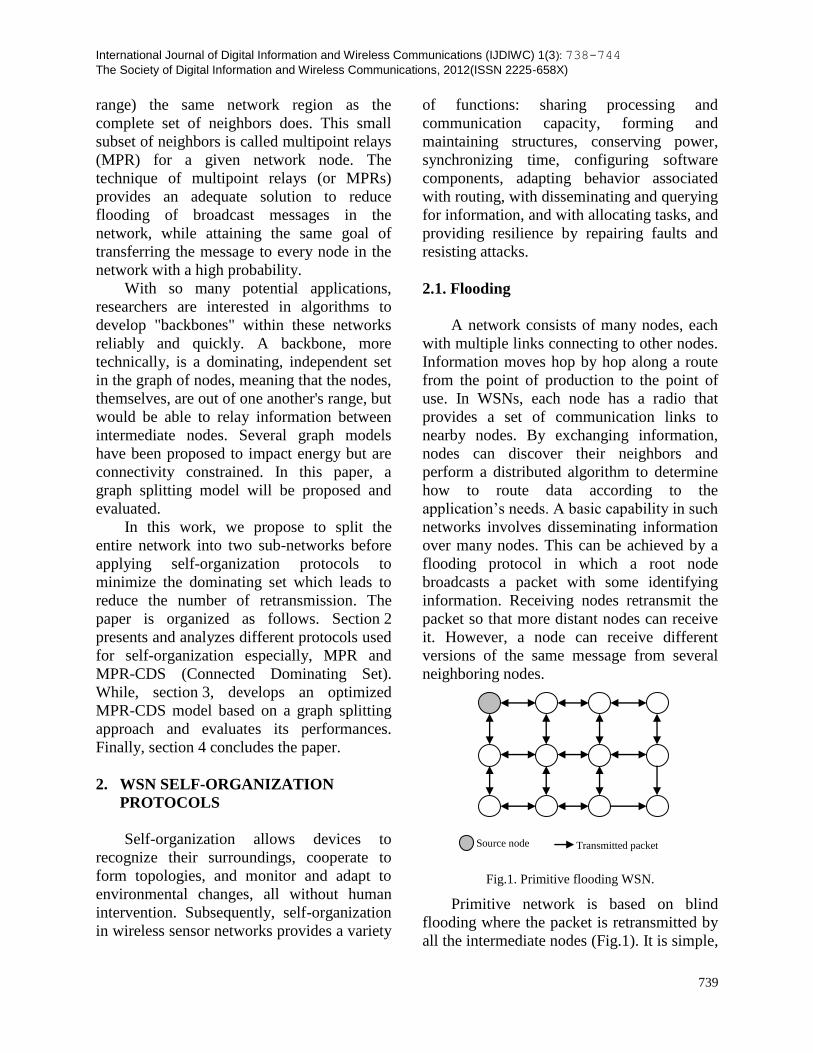
International Journal of Digital Information and Wireless Communications (IJDIWC) 1(3): 738-744
The Society of Digital Information and Wireless Communications, 2012(ISSN 2225-658X)
739
range) the same network region as the
complete set of neighbors does. This small
subset of neighbors is called multipoint relays
(MPR) for a given network node. The
technique of multipoint relays (or MPRs)
provides an adequate solution to reduce
flooding of broadcast messages in the
network, while attaining the same goal of
transferring the message to every node in the
network with a high probability.
With so many potential applications,
researchers are interested in algorithms to
develop "backbones" within these networks
reliably and quickly. A backbone, more
technically, is a dominating, independent set
in the graph of nodes, meaning that the nodes,
themselves, are out of one another's range, but
would be able to relay information between
intermediate nodes. Several graph models
have been proposed to impact energy but are
connectivity constrained. In this paper, a
graph splitting model will be proposed and
evaluated.
In this work, we propose to split the
entire network into two sub-networks before
applying self-organization protocols to
minimize the dominating set which leads to
reduce the number of retransmission. The
paper is organized as follows. Section 2
presents and analyzes different protocols used
for self-organization especially, MPR and
MPR-CDS (Connected Dominating Set).
While, section 3, develops an optimized
MPR-CDS model based on a graph splitting
approach and evaluates its performances.
Finally, section 4 concludes the paper.
2. WSN SELF-ORGANIZATION
PROTOCOLS
Self-organization allows devices to
recognize their surroundings, cooperate to
form topologies, and monitor and adapt to
environmental changes, all without human
intervention. Subsequently, self-organization
in wireless sensor networks provides a variety
of functions: sharing processing and
communication capacity, forming and
maintaining structures, conserving power,
synchronizing time, configuring software
components, adapting behavior associated
with routing, with disseminating and querying
for information, and with allocating tasks, and
providing resilience by repairing faults and
resisting attacks.
2.1. Flooding
A network consists of many nodes, each
with multiple links connecting to other nodes.
Information moves hop by hop along a route
from the point of production to the point of
use. In WSNs, each node has a radio that
provides a set of communication links to
nearby nodes. By exchanging information,
nodes can discover their neighbors and
perform a distributed algorithm to determine
how to route data according to the
application’s needs. A basic capability in such
networks involves disseminating information
over many nodes. This can be achieved by a
flooding protocol in which a root node
broadcasts a packet with some identifying
information. Receiving nodes retransmit the
packet so that more distant nodes can receive
it. However, a node can receive different
versions of the same message from several
neighboring nodes.
Fig.1. Primitive flooding WSN.
Primitive network is based on blind
flooding where the packet is retransmitted by
all the intermediate nodes (Fig.1). It is simple,
Source node Transmitted packet
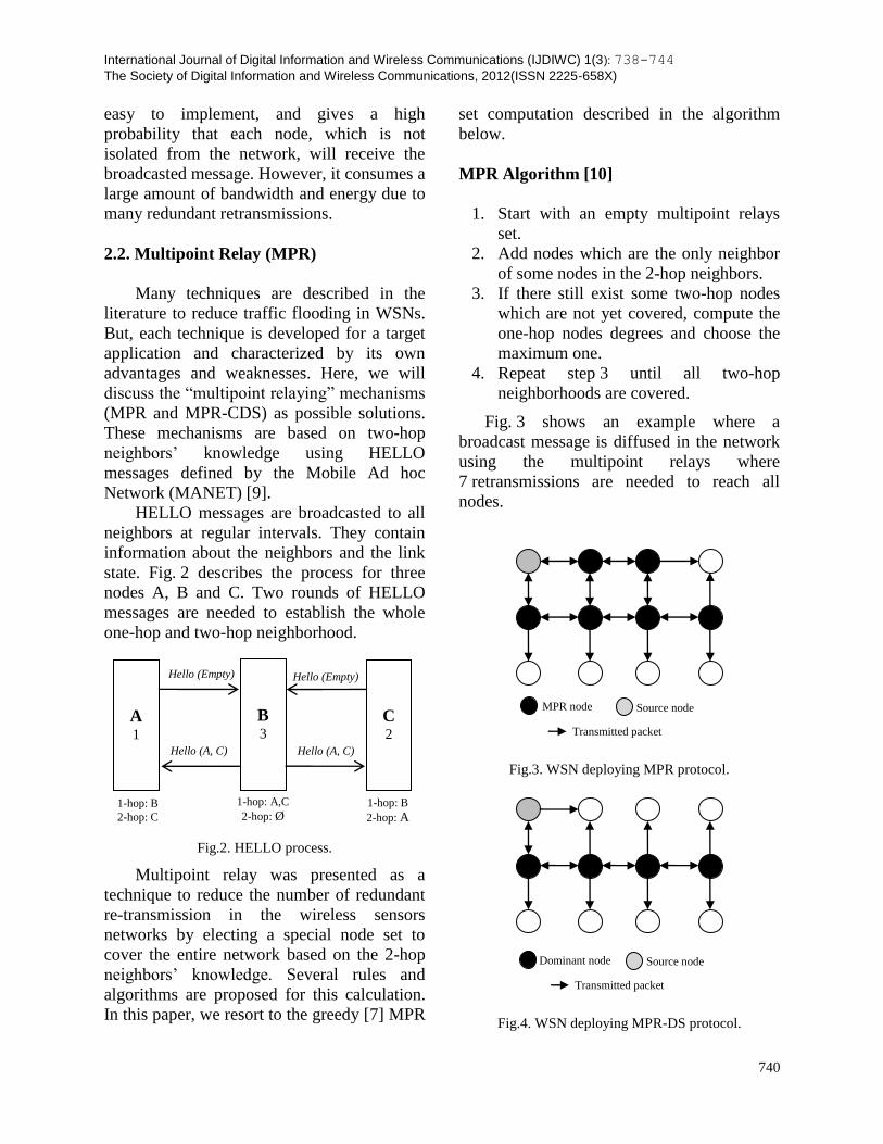
International Journal of Digital Information and Wireless Communications (IJDIWC) 1(3): 738-744
The Society of Digital Information and Wireless Communications, 2012(ISSN 2225-658X)
740
easy to implement, and gives a high
probability that each node, which is not
isolated from the network, will receive the
broadcasted message. However, it consumes a
large amount of bandwidth and energy due to
many redundant retransmissions.
2.2. Multipoint Relay (MPR)
Many techniques are described in the
literature to reduce traffic flooding in WSNs.
But, each technique is developed for a target
application and characterized by its own
advantages and weaknesses. Here, we will
discuss the “multipoint relaying” mechanisms
(MPR and MPR-CDS) as possible solutions.
These mechanisms are based on two-hop
neighbors’ knowledge using HELLO
messages defined by the Mobile Ad hoc
Network (MANET) [9].
HELLO messages are broadcasted to all
neighbors at regular intervals. They contain
information about the neighbors and the link
state. Fig. 2 describes the process for three
nodes A, B and C. Two rounds of HELLO
messages are needed to establish the whole
one-hop and two-hop neighborhood.
Fig.2. HELLO process.
Multipoint relay was presented as a
technique to reduce the number of redundant
re-transmission in the wireless sensors
networks by electing a special node set to
cover the entire network based on the 2-hop
neighbors’ knowledge. Several rules and
algorithms are proposed for this calculation.
In this paper, we resort to the greedy [7] MPR
set computation described in the algorithm
below.
MPR Algorithm [10]
1. Start with an empty multipoint relays
set.
2. Add nodes which are the only neighbor
of some nodes in the 2-hop neighbors.
3. If there still exist some two-hop nodes
which are not yet covered, compute the
one-hop nodes degrees and choose the
maximum one.
4. Repeat step 3 until all two-hop
neighborhoods are covered.
Fig. 3 shows an example where a
broadcast message is diffused in the network
using the multipoint relays where
7 retransmissions are needed to reach all
nodes.
Fig.3. WSN deploying MPR protocol.
Fig.4. WSN deploying MPR-DS protocol.
Dominant node Source node
Transmitted packet
MPR node Source node
Transmitted packet
A 1
B 3
C 2
Hello (Empty) Hello (Empty)
Hello (A, C) Hello (A, C)
1-hop: A,C
2-hop: Ø
1-hop: B
2-hop: A
1-hop: B
2-hop: C
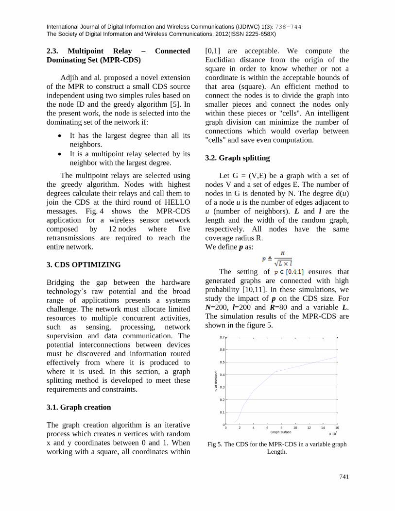
International Journal of Digital Information and Wireless Communications (IJDIWC) 1(3): 738-744
The Society of Digital Information and Wireless Communications, 2012(ISSN 2225-658X)
741
2.3. Multipoint Relay – Connected
Dominating Set (MPR-CDS)
Adjih and al. proposed a novel extension
of the MPR to construct a small CDS source
independent using two simples rules based on
the node ID and the greedy algorithm [5]. In
the present work, the node is selected into the
dominating set of the network if:
It has the largest degree than all its
neighbors.
It is a multipoint relay selected by its
neighbor with the largest degree.
The multipoint relays are selected using
the greedy algorithm. Nodes with highest
degrees calculate their relays and call them to
join the CDS at the third round of HELLO
messages. Fig. 4 shows the MPR-CDS
application for a wireless sensor network
composed by 12 nodes where five
retransmissions are required to reach the
entire network.
3. CDS OPTIMIZING
Bridging the gap between the hardware
technology’s raw potential and the broad
range of applications presents a systems
challenge. The network must allocate limited
resources to multiple concurrent activities,
such as sensing, processing, network
supervision and data communication. The
potential interconnections between devices
must be discovered and information routed
effectively from where it is produced to
where it is used. In this section, a graph
splitting method is developed to meet these
requirements and constraints.
3.1. Graph creation
The graph creation algorithm is an iterative
process which creates n vertices with random
x and y coordinates between 0 and 1. When
working with a square, all coordinates within
[0,1] are acceptable. We compute the
Euclidian distance from the origin of the
square in order to know whether or not a
coordinate is within the acceptable bounds of
that area (square). An efficient method to
connect the nodes is to divide the graph into
smaller pieces and connect the nodes only
within these pieces or "cells". An intelligent
graph division can minimize the number of
connections which would overlap between
"cells" and save even computation.
3.2. Graph splitting
Let G = (V,E) be a graph with a set of
nodes V and a set of edges E. The number of
nodes in G is denoted by N. The degree d(u)
of a node u is the number of edges adjacent to
u (number of neighbors). L and l are the
length and the width of the random graph,
respectively. All nodes have the same
coverage radius R.
We define p as:
The setting of ensures that
generated graphs are connected with high
probability [10,11]. In these simulations, we
study the impact of p on the CDS size. For
N=200, l=200 and R=80 and a variable L.
The simulation results of the MPR-CDS are
shown in the figure 5.
0 2 4 6 8 10 12 14 16
x 104
0
0.1
0.2
0.3
0.4
0.5
0.6
0.7
Graph surface
% o
f dom
inant
Fig 5. The CDS for the MPR-CDS in a variable graph
Length.
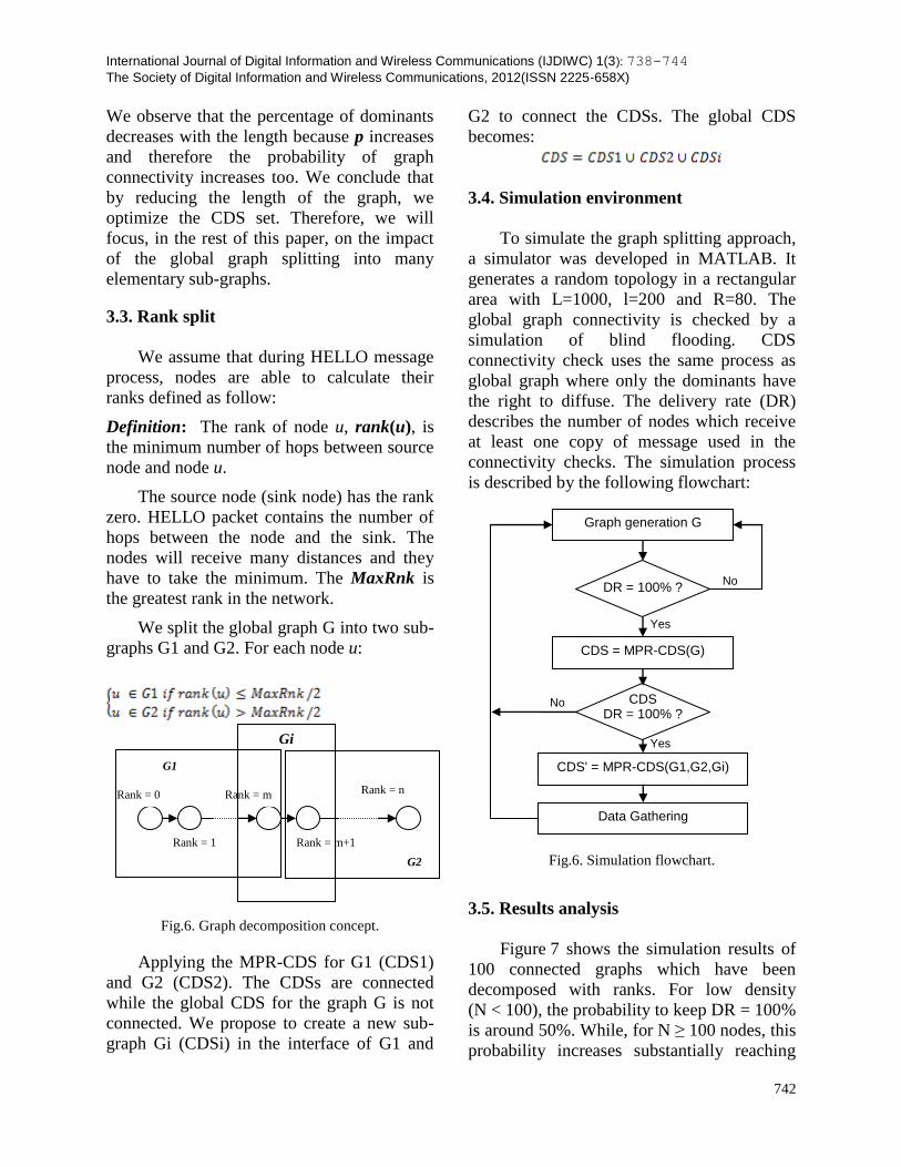
International Journal of Digital Information and Wireless Communications (IJDIWC) 1(3): 738-744
The Society of Digital Information and Wireless Communications, 2012(ISSN 2225-658X)
742
We observe that the percentage of dominants
decreases with the length because p increases
and therefore the probability of graph
connectivity increases too. We conclude that
by reducing the length of the graph, we
optimize the CDS set. Therefore, we will
focus, in the rest of this paper, on the impact
of the global graph splitting into many
elementary sub-graphs.
3.3. Rank split
We assume that during HELLO message
process, nodes are able to calculate their
ranks defined as follow:
Definition: The rank of node u, rank(u), is
the minimum number of hops between source
node and node u.
The source node (sink node) has the rank
zero. HELLO packet contains the number of
hops between the node and the sink. The
nodes will receive many distances and they
have to take the minimum. The MaxRnk is
the greatest rank in the network.
We split the global graph G into two sub-
graphs G1 and G2. For each node u:
Fig.6. Graph decomposition concept.
Applying the MPR-CDS for G1 (CDS1)
and G2 (CDS2). The CDSs are connected
while the global CDS for the graph G is not
connected. We propose to create a new sub-
graph Gi (CDSi) in the interface of G1 and
G2 to connect the CDSs. The global CDS
becomes:
3.4. Simulation environment
To simulate the graph splitting approach,
a simulator was developed in MATLAB. It
generates a random topology in a rectangular
area with L=1000, l=200 and R=80. The
global graph connectivity is checked by a
simulation of blind flooding. CDS
connectivity check uses the same process as
global graph where only the dominants have
the right to diffuse. The delivery rate (DR)
describes the number of nodes which receive
at least one copy of message used in the
connectivity checks. The simulation process
is described by the following flowchart:
Fig.6. Simulation flowchart.
3.5. Results analysis
Figure 7 shows the simulation results of
100 connected graphs which have been
decomposed with ranks. For low density
(N < 100), the probability to keep DR = 100%
is around 50%. While, for N ≥ 100 nodes, this
probability increases substantially reaching
Rank = 0
Rank = 1
Rank = m
Rank = m+1
Rank = n
G1
G2
Gi
Graph generation G
DR = 100% ?
CDS = MPR-CDS(G)
CDS DR = 100% ?
CDS' = MPR-CDS(G1,G2,Gi)
Data Gathering
No
No
Yes
Yes
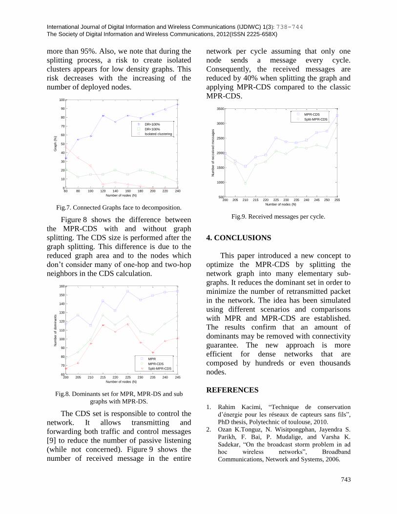
International Journal of Digital Information and Wireless Communications (IJDIWC) 1(3): 738-744
The Society of Digital Information and Wireless Communications, 2012(ISSN 2225-658X)
743
more than 95%. Also, we note that during the
splitting process, a risk to create isolated
clusters appears for low density graphs. This
risk decreases with the increasing of the
number of deployed nodes.
60 80 100 120 140 160 180 200 220 2400
10
20
30
40
50
60
70
80
90
100
Number of nodes (N)
Gra
ph (
%)
DR=100%
DR<100%
Isolated clustering
Fig.7. Connected Graphs face to decomposition.
Figure 8 shows the difference between
the MPR-CDS with and without graph
splitting. The CDS size is performed after the
graph splitting. This difference is due to the
reduced graph area and to the nodes which
don’t consider many of one-hop and two-hop
neighbors in the CDS calculation.
200 205 210 215 220 225 230 235 240 24560
70
80
90
100
110
120
130
140
150
160
Number of nodes (N)
Num
ber
of
dom
inants
MPR
MPR-CDS
Split-MPR-CDS
Fig.8. Dominants set for MPR, MPR-DS and sub
graphs with MPR-DS.
The CDS set is responsible to control the
network. It allows transmitting and
forwarding both traffic and control messages
[9] to reduce the number of passive listening
(while not concerned). Figure 9 shows the
number of received message in the entire
network per cycle assuming that only one
node sends a message every cycle.
Consequently, the received messages are
reduced by 40% when splitting the graph and
applying MPR-CDS compared to the classic
MPR-CDS.
200 205 210 215 220 225 230 235 240 245 250 255500
1000
1500
2000
2500
3000
3500
Number of nodes (N)
Num
ber
of
recceiv
ed m
essages
MPR-CDS
Split-MPR-CDS
Fig.9. Received messages per cycle.
4. CONCLUSIONS
This paper introduced a new concept to
optimize the MPR-CDS by splitting the
network graph into many elementary sub-
graphs. It reduces the dominant set in order to
minimize the number of retransmitted packet
in the network. The idea has been simulated
using different scenarios and comparisons
with MPR and MPR-CDS are established.
The results confirm that an amount of
dominants may be removed with connectivity
guarantee. The new approach is more
efficient for dense networks that are
composed by hundreds or even thousands
nodes.
REFERENCES
1. Rahim Kacimi, “Technique de conservation
d’énergie pour les réseaux de capteurs sans fils”,
PhD thesis, Polytechnic of toulouse, 2010.
2. Ozan K.Tonguz, N. Wisitpongphan, Jayendra S.
Parikh, F. Bai, P. Mudalige, and Varsha K.
Sadekar, “On the broadcast storm problem in ad
hoc wireless networks”, Broadband
Communications, Network and Systems, 2006.
International Journal of Digital Information and Wireless Communications (IJDIWC) 1(3): 738-744
The Society of Digital Information and Wireless Communications, 2012(ISSN 2225-658X)
744
3. Karel Heurtefeux and Fabrice Valois, “self-
organization protocols: behavior during the sensor
networks life”, The 18th Annual IEEE
International Symposium on Personal, Indoor and
Mobile Radio Communications, 2007.
4. Jie Wu, Wei Lou and Fei Dai, “Extended
Multipoint relays to determine connected
dominating sets in MANET’s”, IEEE transaction
on computer, vol. 55, NO. 3, MARCH 2006.
5. Xiao chen and Jian Shen, “Reducing connected
dominating set size with multipoint relays in ad
hoc wireless networks”, Proceed. of the 7th
international Symposium on parallel architecture,
algorithms and networks, 2004.
6. Rajiv Misra, “On self-stabilization of multipoint
relays for connected dominating set in ad hoc
networks”, IEEE region 10 conference, TENCON
2009.
7. Yongsheng Fu, Xinyu Wang, Wei Shi and
Shanping Li, “Connectivity based greedy
algorithm with multipoint relaying for mobile ad
hoc networks”, The 4th international conference
on mobile ad-hoc and sensor network, 2008.
8. Cedric Adjih, philipe Jacquet and Laurent
Viennot, “Computing connected dominated sets
with multipoint relays”, Technical report, INRIA,
Oct.2002, www.inria.fr/rrrt/rr-4597.html.
9. T.Claussen, P.Jacquet, C. Adjih, A. Laouiti, P.
Minet,P. Muhlethaler,A. Quayyam and L. Viennot,
“Optimized link state routing protocol (OLSR)”,
RFC 3626, Oct. 2003, Network Working Group.
10. C. Bettestetter, “On the minimum node degree and
connectivity of a wireless multi-hop network”, in
Proc. ACM MobiHoc, Lausanne, Switzerland, Jun.
2002.
11. S. Crisostomo, J.Barros and C. Bettstetter,
“Flooding the network: Multipoint relays versus
network coding”, Circuits and Systems for
Communications, 2008.
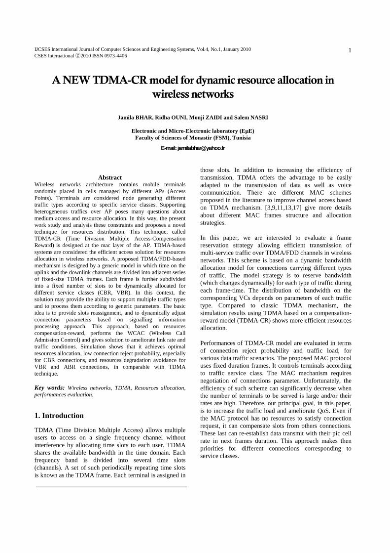
IJCSES International Journal of Computer Sciences and Engineering Systems, Vol.4, No.1, January 2010 CSES International ⓒ2010 ISSN 0973-4406
1
A NEW TDMA-CR model for dynamic resource allocation in
wireless networks
Jamila BHAR, Ridha OUNI, Monji ZAIDI and Salem NASR I
Electronic and Micro-Electronic laboratory (EµE) Faculty of Sciences of Monastir (FSM), Tunisia
E-mail: [email protected]
Abstract
Wireless networks architecture contains mobile terminals randomly placed in cells managed by different APs (Access Points). Terminals are considered node generating different traffic types according to specific service classes. Supporting heterogeneous traffics over AP poses many questions about medium access and resource allocation. In this way, the present work study and analysis these constraints and proposes a novel technique for resources distribution. This technique, called TDMA-CR (Time Division Multiple Access-Compensation Reward) is designed at the mac layer of the AP. TDMA-based systems are considered the efficient access solution for resources allocation in wireless networks. A proposed TDMA/FDD-based mechanism is designed by a generic model in which time on the uplink and the downlink channels are divided into adjacent series of fixed-size TDMA frames. Each frame is further subdivided into a fixed number of slots to be dynamically allocated for different service classes (CBR, VBR). In this context, the solution may provide the ability to support multiple traffic types and to process them according to generic parameters. The basic idea is to provide slots reassignment, and to dynamically adjust connection parameters based on signalling information processing approach. This approach, based on resources compensation-reward, performs the WCAC (Wireless Call Admission Control) and gives solution to ameliorate link rate and traffic conditions. Simulation shows that it achieves optimal resources allocation, low connection reject probability, especially for CBR connections, and resources degradation avoidance for VBR and ABR connections, in comparable with TDMA technique. Key words: Wireless networks, TDMA, Resources allocation, performances evaluation.
1. Introduction
TDMA (Time Division Multiple Access) allows multiple users to access on a single frequency channel without interference by allocating time slots to each user. TDMA shares the available bandwidth in the time domain. Each frequency band is divided into several time slots (channels). A set of such periodically repeating time slots is known as the TDMA frame. Each terminal is assigned in
those slots. In addition to increasing the efficiency of transmission, TDMA offers the advantage to be easily adapted to the transmission of data as well as voice communication. There are different MAC schemes proposed in the literature to improve channel access based on TDMA mechanism. [3,9,11,13,17] give more details about different MAC frames structure and allocation strategies. In this paper, we are interested to evaluate a frame reservation strategy allowing efficient transmission of multi-service traffic over TDMA/FDD channels in wireless networks. This scheme is based on a dynamic bandwidth allocation model for connections carrying different types of traffic. The model strategy is to reserve bandwidth (which changes dynamically) for each type of traffic during each frame-time. The distribution of bandwidth on the corresponding VCs depends on parameters of each traffic type. Compared to classic TDMA mechanism, the simulation results using TDMA based on a compensation-reward model (TDMA-CR) shows more efficient resources allocation. Performances of TDMA-CR model are evaluated in terms of connection reject probability and traffic load, for various data traffic scenarios. The proposed MAC protocol uses fixed duration frames. It controls terminals according to traffic service class. The MAC mechanism requires negotiation of connections parameter. Unfortunately, the efficiency of such scheme can significantly decrease when the number of terminals to be served is large and/or their rates are high. Therefore, our principal goal, in this paper, is to increase the traffic load and ameliorate QoS. Even if the MAC protocol has no resources to satisfy connection request, it can compensate slots from others connections. These last can re-establish data transmit with their pic cell rate in next frames duration. This approach makes then priorities for different connections corresponding to service classes.
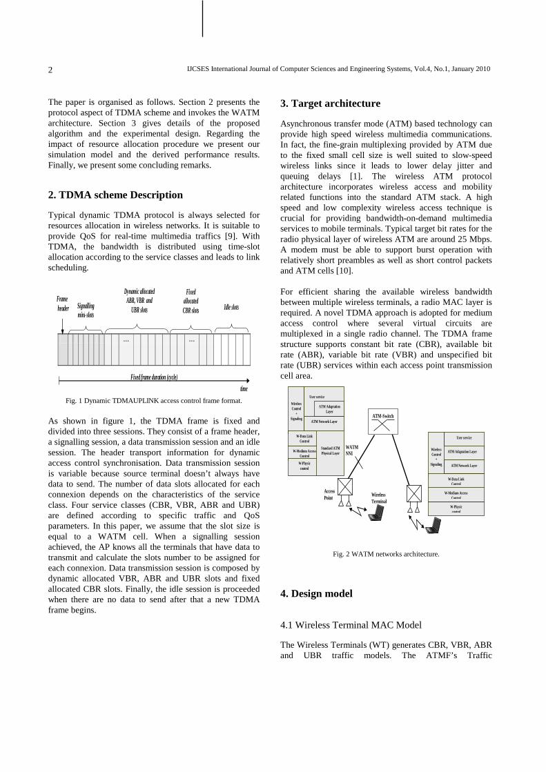
IJCSES International Journal of Computer Sciences and Engineering Systems, Vol.4, No.1, January 2010
2
The paper is organised as follows. Section 2 presents the protocol aspect of TDMA scheme and invokes the WATM architecture. Section 3 gives details of the proposed algorithm and the experimental design. Regarding the impact of resource allocation procedure we present our simulation model and the derived performance results. Finally, we present some concluding remarks.
2. TDMA scheme Description
Typical dynamic TDMA protocol is always selected for resources allocation in wireless networks. It is suitable to provide QoS for real-time multimedia traffics [9]. With TDMA, the bandwidth is distributed using time-slot allocation according to the service classes and leads to link scheduling.
time
Fixed frame duration (cycle)
. . . . . .
Frame header Signalling
mini-slots
Dynamic allocated ABR, VBR and
UBR slots
Fixed allocated CBR slots Idle slots
Fig. 1 Dynamic TDMAUPLINK access control frame format.
As shown in figure 1, the TDMA frame is fixed and divided into three sessions. They consist of a frame header, a signalling session, a data transmission session and an idle session. The header transport information for dynamic access control synchronisation. Data transmission session is variable because source terminal doesn’t always have data to send. The number of data slots allocated for each connexion depends on the characteristics of the service class. Four service classes (CBR, VBR, ABR and UBR) are defined according to specific traffic and QoS parameters. In this paper, we assume that the slot size is equal to a WATM cell. When a signalling session achieved, the AP knows all the terminals that have data to transmit and calculate the slots number to be assigned for each connexion. Data transmission session is composed by dynamic allocated VBR, ABR and UBR slots and fixed allocated CBR slots. Finally, the idle session is proceeded when there are no data to send after that a new TDMA frame begins.
3. Target architecture
Asynchronous transfer mode (ATM) based technology can provide high speed wireless multimedia communications. In fact, the fine-grain multiplexing provided by ATM due to the fixed small cell size is well suited to slow-speed wireless links since it leads to lower delay jitter and queuing delays [1]. The wireless ATM protocol architecture incorporates wireless access and mobility related functions into the standard ATM stack. A high speed and low complexity wireless access technique is crucial for providing bandwidth-on-demand multimedia services to mobile terminals. Typical target bit rates for the radio physical layer of wireless ATM are around 25 Mbps. A modem must be able to support burst operation with relatively short preambles as well as short control packets and ATM cells [10]. For efficient sharing the available wireless bandwidth between multiple wireless terminals, a radio MAC layer is required. A novel TDMA approach is adopted for medium access control where several virtual circuits are multiplexed in a single radio channel. The TDMA frame structure supports constant bit rate (CBR), available bit rate (ABR), variable bit rate (VBR) and unspecified bit rate (UBR) services within each access point transmission cell area.
Wireless Control
+ Signaling
W-Data Link Control
W-Medium Access Control
W-Physic control
Standard ATM Physical Layer
User service
ATM Network Layer
ATM Adaptation Layer
User service
ATM Network Layer
ATM Adaptation Layer
W-Physic control
W-Medium Access Control
Wireless Control
+ Signaling
W-Data Link Control
WATM NNI
ATM-Switch
Wireless Terminal
Access Point
Fig. 2 WATM networks architecture.
4. Design model
4.1 Wireless Terminal MAC Model
The Wireless Terminals (WT) generates CBR, VBR, ABR and UBR traffic models. The ATMF’s Traffic
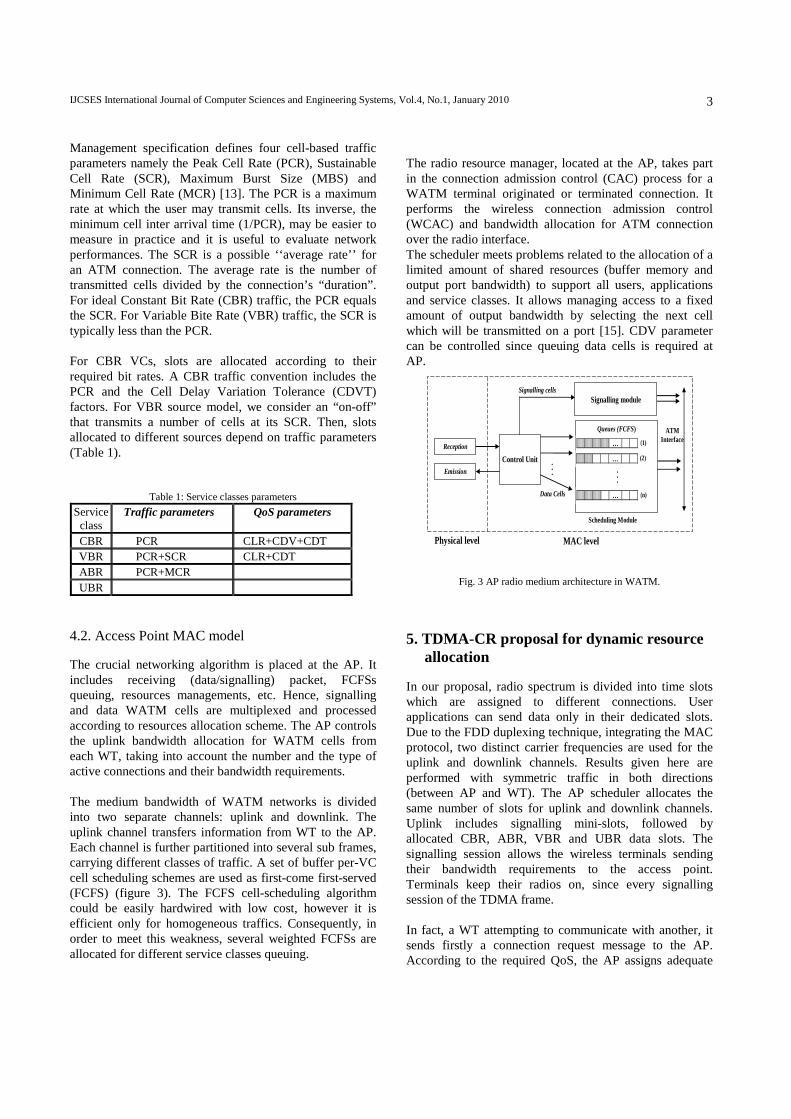
IJCSES International Journal of Computer Sciences and Engineering Systems, Vol.4, No.1, January 2010
3
Management specification defines four cell-based traffic parameters namely the Peak Cell Rate (PCR), Sustainable Cell Rate (SCR), Maximum Burst Size (MBS) and Minimum Cell Rate (MCR) [13]. The PCR is a maximum rate at which the user may transmit cells. Its inverse, the minimum cell inter arrival time (1/PCR), may be easier to measure in practice and it is useful to evaluate network performances. The SCR is a possible ‘‘average rate’’ for an ATM connection. The average rate is the number of transmitted cells divided by the connection’s “duration”. For ideal Constant Bit Rate (CBR) traffic, the PCR equals the SCR. For Variable Bite Rate (VBR) traffic, the SCR is typically less than the PCR. For CBR VCs, slots are allocated according to their required bit rates. A CBR traffic convention includes the PCR and the Cell Delay Variation Tolerance (CDVT) factors. For VBR source model, we consider an “on-off” that transmits a number of cells at its SCR. Then, slots allocated to different sources depend on traffic parameters (Table 1).
Table 1: Service classes parameters
Service class
Traffic parameters QoS parameters
CBR PCR CLR+CDV+CDT VBR PCR+SCR CLR+CDT ABR PCR+MCR UBR
4.2. Access Point MAC model
The crucial networking algorithm is placed at the AP. It includes receiving (data/signalling) packet, FCFSs queuing, resources managements, etc. Hence, signalling and data WATM cells are multiplexed and processed according to resources allocation scheme. The AP controls the uplink bandwidth allocation for WATM cells from each WT, taking into account the number and the type of active connections and their bandwidth requirements. The medium bandwidth of WATM networks is divided into two separate channels: uplink and downlink. The uplink channel transfers information from WT to the AP. Each channel is further partitioned into several sub frames, carrying different classes of traffic. A set of buffer per-VC cell scheduling schemes are used as first-come first-served (FCFS) (figure 3). The FCFS cell-scheduling algorithm could be easily hardwired with low cost, however it is efficient only for homogeneous traffics. Consequently, in order to meet this weakness, several weighted FCFSs are allocated for different service classes queuing.
The radio resource manager, located at the AP, takes part in the connection admission control (CAC) process for a WATM terminal originated or terminated connection. It performs the wireless connection admission control (WCAC) and bandwidth allocation for ATM connection over the radio interface. The scheduler meets problems related to the allocation of a limited amount of shared resources (buffer memory and output port bandwidth) to support all users, applications and service classes. It allows managing access to a fixed amount of output bandwidth by selecting the next cell which will be transmitted on a port [15]. CDV parameter can be controlled since queuing data cells is required at AP.
ATM Interface
Data Cells
Scheduling Module
Queues (FCFS)
(2)
(n)
(1)
Signalling cells
Reception
Emission
Control Unit
…
. .
.
...
Signalling module
MAC level Physical level
…
…
Fig. 3 AP radio medium architecture in WATM.
5. TDMA-CR proposal for dynamic resource allocation
In our proposal, radio spectrum is divided into time slots which are assigned to different connections. User applications can send data only in their dedicated slots. Due to the FDD duplexing technique, integrating the MAC protocol, two distinct carrier frequencies are used for the uplink and downlink channels. Results given here are performed with symmetric traffic in both directions (between AP and WT). The AP scheduler allocates the same number of slots for uplink and downlink channels. Uplink includes signalling mini-slots, followed by allocated CBR, ABR, VBR and UBR data slots. The signalling session allows the wireless terminals sending their bandwidth requirements to the access point. Terminals keep their radios on, since every signalling session of the TDMA frame. In fact, a WT attempting to communicate with another, it sends firstly a connection request message to the AP. According to the required QoS, the AP assigns adequate
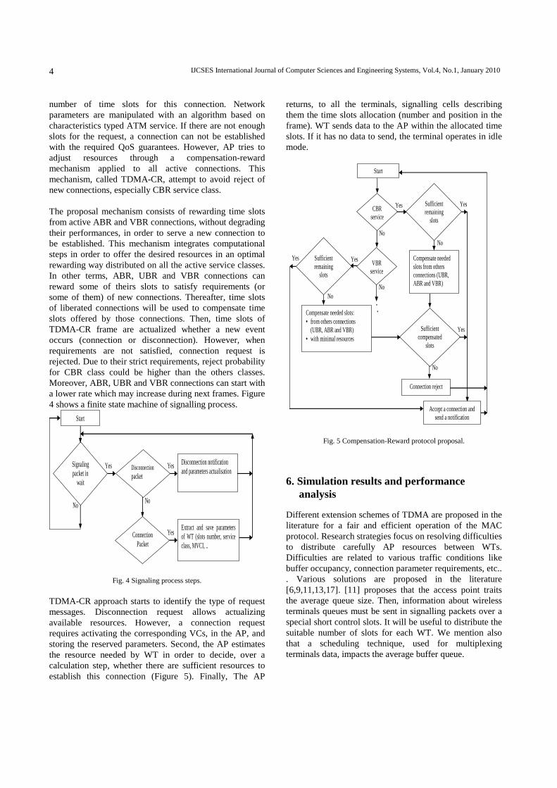
IJCSES International Journal of Computer Sciences and Engineering Systems, Vol.4, No.1, January 2010
4
number of time slots for this connection. Network parameters are manipulated with an algorithm based on characteristics typed ATM service. If there are not enough slots for the request, a connection can not be established with the required QoS guarantees. However, AP tries to adjust resources through a compensation-reward mechanism applied to all active connections. This mechanism, called TDMA-CR, attempt to avoid reject of new connections, especially CBR service class. The proposal mechanism consists of rewarding time slots from active ABR and VBR connections, without degrading their performances, in order to serve a new connection to be established. This mechanism integrates computational steps in order to offer the desired resources in an optimal rewarding way distributed on all the active service classes. In other terms, ABR, UBR and VBR connections can reward some of theirs slots to satisfy requirements (or some of them) of new connections. Thereafter, time slots of liberated connections will be used to compensate time slots offered by those connections. Then, time slots of TDMA-CR frame are actualized whether a new event occurs (connection or disconnection). However, when requirements are not satisfied, connection request is rejected. Due to their strict requirements, reject probability for CBR class could be higher than the others classes. Moreover, ABR, UBR and VBR connections can start with a lower rate which may increase during next frames. Figure 4 shows a finite state machine of signalling process.
Yes Yes Signaling packet in
wait
Start
No
Disconnection packet
Disconnection notification and parameters actualisation
No
Yes Connection Packet
Extract and save parameters of WT (slots number, service class, MVCI, ..
Fig. 4 Signaling process steps.
TDMA-CR approach starts to identify the type of request messages. Disconnection request allows actualizing available resources. However, a connection request requires activating the corresponding VCs, in the AP, and storing the reserved parameters. Second, the AP estimates the resource needed by WT in order to decide, over a calculation step, whether there are sufficient resources to establish this connection (Figure 5). Finally, The AP
returns, to all the terminals, signalling cells describing them the time slots allocation (number and position in the frame). WT sends data to the AP within the allocated time slots. If it has no data to send, the terminal operates in idle mode.
Yes Yes
. .
No
No
No
Yes
Yes
No
CBR service
Sufficient remaining
slots
No
Yes Sufficient remaining
slots
Connection reject
Start
Compensate needed slots from others connections (UBR, ABR and VBR)
Sufficient compensated
slots
VBR service
Compensate needed slots: • from others connections
(UBR, ABR and VBR) • with minimal resources
Accept a connection and send a notification
Fig. 5 Compensation-Reward protocol proposal.
6. Simulation results and performance analysis
Different extension schemes of TDMA are proposed in the literature for a fair and efficient operation of the MAC protocol. Research strategies focus on resolving difficulties to distribute carefully AP resources between WTs. Difficulties are related to various traffic conditions like buffer occupancy, connection parameter requirements, etc.. . Various solutions are proposed in the literature [6,9,11,13,17]. [11] proposes that the access point traits the average queue size. Then, information about wireless terminals queues must be sent in signalling packets over a special short control slots. It will be useful to distribute the suitable number of slots for each WT. We mention also that a scheduling technique, used for multiplexing terminals data, impacts the average buffer queue.
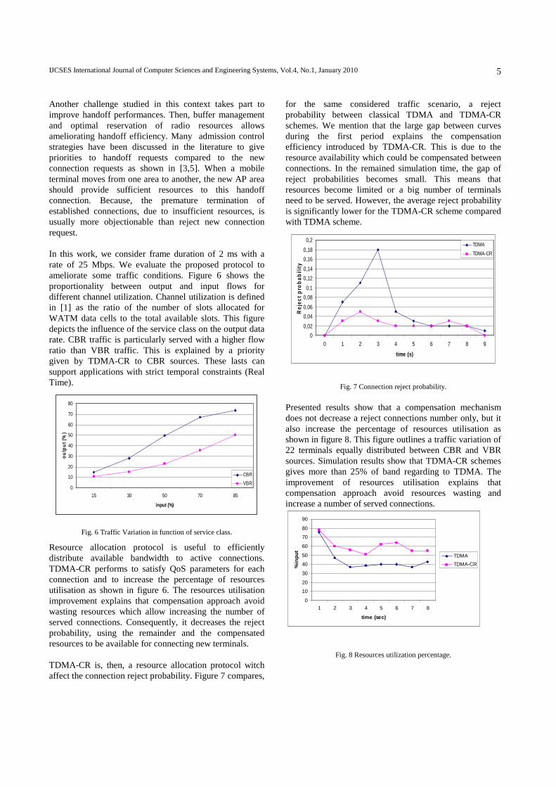
IJCSES International Journal of Computer Sciences and Engineering Systems, Vol.4, No.1, January 2010
5
Another challenge studied in this context takes part to improve handoff performances. Then, buffer management and optimal reservation of radio resources allows ameliorating handoff efficiency. Many admission control strategies have been discussed in the literature to give priorities to handoff requests compared to the new connection requests as shown in [3,5]. When a mobile terminal moves from one area to another, the new AP area should provide sufficient resources to this handoff connection. Because, the premature termination of established connections, due to insufficient resources, is usually more objectionable than reject new connection request. In this work, we consider frame duration of 2 ms with a rate of 25 Mbps. We evaluate the proposed protocol to ameliorate some traffic conditions. Figure 6 shows the proportionality between output and input flows for different channel utilization. Channel utilization is defined in [1] as the ratio of the number of slots allocated for WATM data cells to the total available slots. This figure depicts the influence of the service class on the output data rate. CBR traffic is particularly served with a higher flow ratio than VBR traffic. This is explained by a priority given by TDMA-CR to CBR sources. These lasts can support applications with strict temporal constraints (Real Time).
0
10
20
30
40
50
60
70
80
15 30 50 70 85
input (%)
outp
ut (
%)
CBR
VBR
Fig. 6 Traffic Variation in function of service class.
Resource allocation protocol is useful to efficiently distribute available bandwidth to active connections. TDMA-CR performs to satisfy QoS parameters for each connection and to increase the percentage of resources utilisation as shown in figure 6. The resources utilisation improvement explains that compensation approach avoid wasting resources which allow increasing the number of served connections. Consequently, it decreases the reject probability, using the remainder and the compensated resources to be available for connecting new terminals. TDMA-CR is, then, a resource allocation protocol witch affect the connection reject probability. Figure 7 compares,
for the same considered traffic scenario, a reject probability between classical TDMA and TDMA-CR schemes. We mention that the large gap between curves during the first period explains the compensation efficiency introduced by TDMA-CR. This is due to the resource availability which could be compensated between connections. In the remained simulation time, the gap of reject probabilities becomes small. This means that resources become limited or a big number of terminals need to be served. However, the average reject probability is significantly lower for the TDMA-CR scheme compared with TDMA scheme.
0
0,02
0,04
0,06
0,08
0,1
0,12
0,14
0,16
0,18
0,2
0 1 2 3 4 5 6 7 8 9
time (s)
Rej
ect
pro
bab
ility
TDMA
TDMA-CR
Fig. 7 Connection reject probability.
Presented results show that a compensation mechanism does not decrease a reject connections number only, but it also increase the percentage of resources utilisation as shown in figure 8. This figure outlines a traffic variation of 22 terminals equally distributed between CBR and VBR sources. Simulation results show that TDMA-CR schemes gives more than 25% of band regarding to TDMA. The improvement of resources utilisation explains that compensation approach avoid resources wasting and increase a number of served connections.
0
10
20
30
40
50
60
70
80
90
1 2 3 4 5 6 7 8
time (sec)
%in
put
TDMA
TDMA-CR
Fig. 8 Resources utilization percentage.
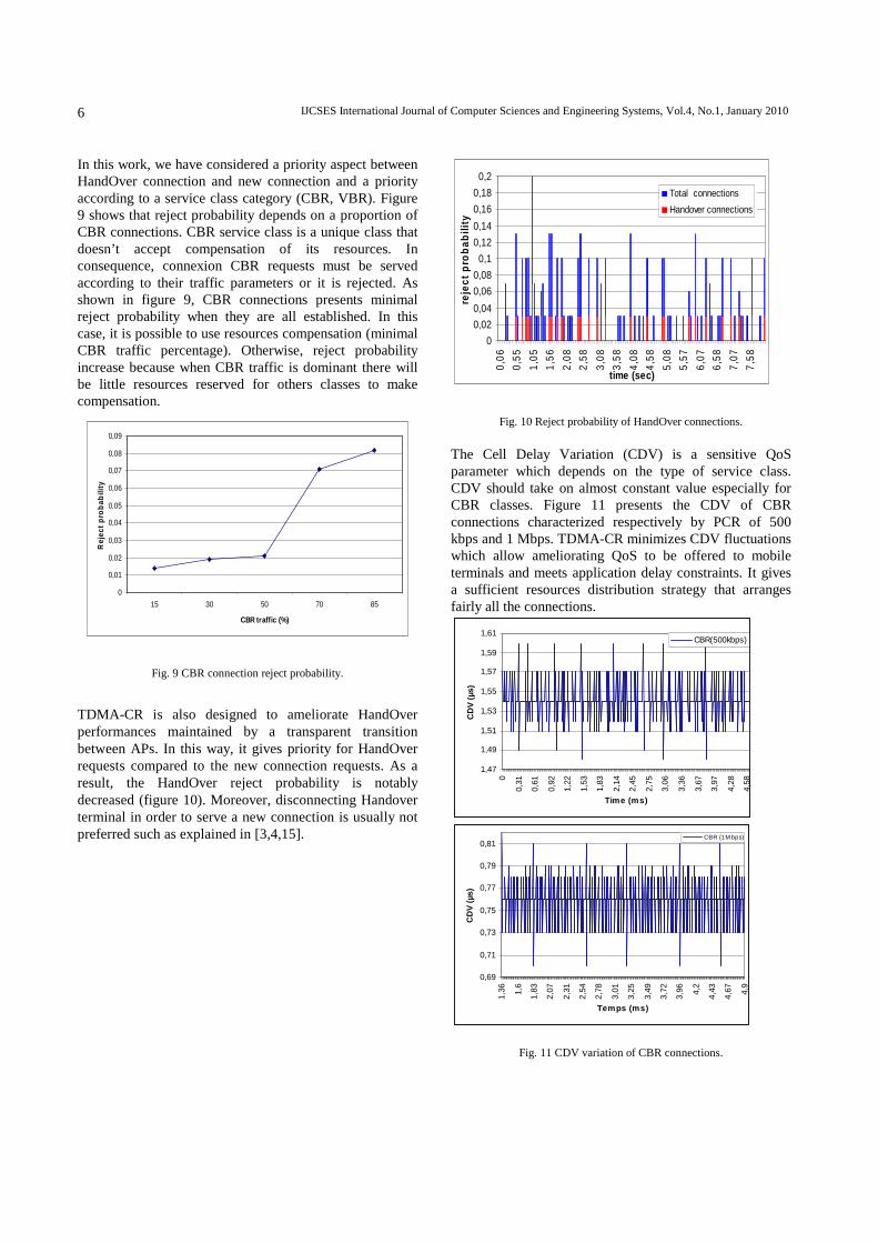
IJCSES International Journal of Computer Sciences and Engineering Systems, Vol.4, No.1, January 2010
6
In this work, we have considered a priority aspect between HandOver connection and new connection and a priority according to a service class category (CBR, VBR). Figure 9 shows that reject probability depends on a proportion of CBR connections. CBR service class is a unique class that doesn’t accept compensation of its resources. In consequence, connexion CBR requests must be served according to their traffic parameters or it is rejected. As shown in figure 9, CBR connections presents minimal reject probability when they are all established. In this case, it is possible to use resources compensation (minimal CBR traffic percentage). Otherwise, reject probability increase because when CBR traffic is dominant there will be little resources reserved for others classes to make compensation.
0
0,01
0,02
0,03
0,04
0,05
0,06
0,07
0,08
0,09
15 30 50 70 85
CBR traffic (%)
Rej
ect p
roba
bilit
y
Fig. 9 CBR connection reject probability.
TDMA-CR is also designed to ameliorate HandOver performances maintained by a transparent transition between APs. In this way, it gives priority for HandOver requests compared to the new connection requests. As a result, the HandOver reject probability is notably decreased (figure 10). Moreover, disconnecting Handover terminal in order to serve a new connection is usually not preferred such as explained in [3,4,15].
0
0,02
0,04
0,06
0,08
0,1
0,12
0,14
0,16
0,18
0,2
0,06
0,55
1,05
1,56
2,08
2,58
3,08
3,58
4,08
4,58
5,08
5,57
6,07
6,58
7,07
7,58
time (sec)
reje
ct p
roba
bilit
y
Total connections
Handover connections
Fig. 10 Reject probability of HandOver connections.
The Cell Delay Variation (CDV) is a sensitive QoS parameter which depends on the type of service class. CDV should take on almost constant value especially for CBR classes. Figure 11 presents the CDV of CBR connections characterized respectively by PCR of 500 kbps and 1 Mbps. TDMA-CR minimizes CDV fluctuations which allow ameliorating QoS to be offered to mobile terminals and meets application delay constraints. It gives a sufficient resources distribution strategy that arranges fairly all the connections.
1,47
1,49
1,51
1,53
1,55
1,57
1,59
1,61
0
0,31
0,61
0,92
1,22
1,53
1,83
2,14
2,45
2,75
3,06
3,36
3,67
3,97
4,28
4,58
Time (ms)
CD
V (
µs)
CBR(500kbps)
0,69
0,71
0,73
0,75
0,77
0,79
0,81
1,36 1,6
1,83
2,07
2,31
2,54
2,78
3,01
3,25
3,49
3,72
3,96 4,2
4,43
4,67 4,9
Temps (ms)
CD
V (
µs)
CBR (1 M bps)
Fig. 11 CDV variation of CBR connections.
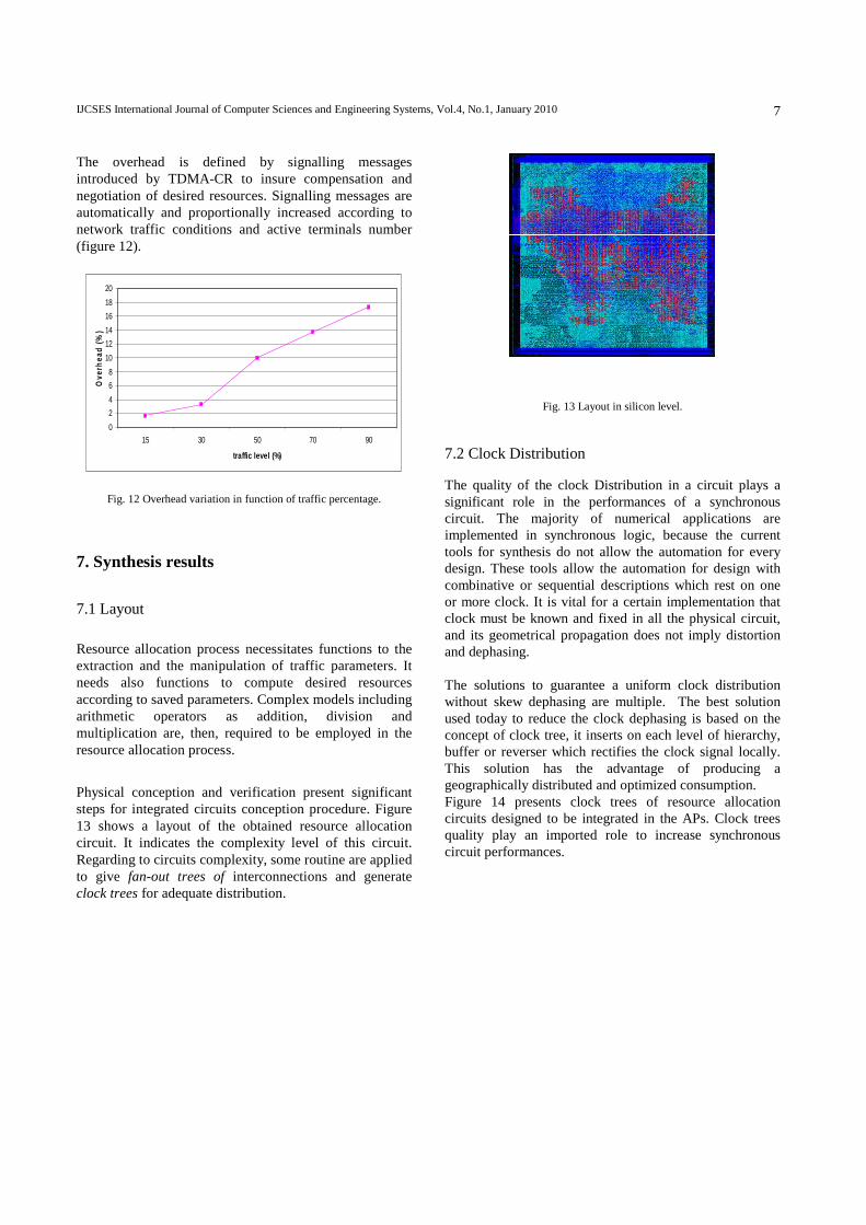
IJCSES International Journal of Computer Sciences and Engineering Systems, Vol.4, No.1, January 2010
7
The overhead is defined by signalling messages introduced by TDMA-CR to insure compensation and negotiation of desired resources. Signalling messages are automatically and proportionally increased according to network traffic conditions and active terminals number (figure 12).
0
2
4
6
8
10
12
14
16
18
20
15 30 50 70 90
traffic level (%)
Ove
rhea
d (%
)
Fig. 12 Overhead variation in function of traffic percentage.
7. Synthesis results
7.1 Layout
Resource allocation process necessitates functions to the extraction and the manipulation of traffic parameters. It needs also functions to compute desired resources according to saved parameters. Complex models including arithmetic operators as addition, division and multiplication are, then, required to be employed in the resource allocation process.
Physical conception and verification present significant steps for integrated circuits conception procedure. Figure 13 shows a layout of the obtained resource allocation circuit. It indicates the complexity level of this circuit. Regarding to circuits complexity, some routine are applied to give fan-out trees of interconnections and generate clock trees for adequate distribution.
Fig. 13 Layout in silicon level.
7.2 Clock Distribution
The quality of the clock Distribution in a circuit plays a significant role in the performances of a synchronous circuit. The majority of numerical applications are implemented in synchronous logic, because the current tools for synthesis do not allow the automation for every design. These tools allow the automation for design with combinative or sequential descriptions which rest on one or more clock. It is vital for a certain implementation that clock must be known and fixed in all the physical circuit, and its geometrical propagation does not imply distortion and dephasing. The solutions to guarantee a uniform clock distribution without skew dephasing are multiple. The best solution used today to reduce the clock dephasing is based on the concept of clock tree, it inserts on each level of hierarchy, buffer or reverser which rectifies the clock signal locally. This solution has the advantage of producing a geographically distributed and optimized consumption. Figure 14 presents clock trees of resource allocation circuits designed to be integrated in the APs. Clock trees quality play an imported role to increase synchronous circuit performances.
IJCSES International Journal of Computer Sciences and Engineering Systems, Vol.4, No.1, January 2010
8
Fig. 14 Clock tree in silicon level.
8. Conclusions
The MAC level should provide QoS management based bandwidth allocation to multiple traffic classes. In fact, various applications such as voice, video and high quality multimedia services need QoS guarantees in order to ensure delay constraints, prescribed data rate and loss. In this paper we have evaluated an algorithm to distribute the resources provided by the access point (AP) at the MAC layer in wireless networks. We consider a classical TDMA/FDD mechanism. It is designed by a generic model in which time on the uplink and downlink channels are divided into a contiguous sequence of fixed-size TDMA frames. Each frame is further subdivided into a fixed number of slots to be dynamically allocated to different ATM traffic classes: CBR, VBR, ABR, and UBR. This approach uses a compensation-reward process called TDMA-CR. It controls all signalling information of connected terminals in order to compute the suitable allocation of slots according to the service classes. Simulation results show the efficiency of such compensation-reward approach to improve traffic conditions.
References [1] Ekram Hossain and Vijay K. Bhargava; Link-Level Traffic
Scheduling for Providing Predictive QoS in Wireless Multimedia Networks; IEEE transactions on multimedia, Vol 6, N°1, Feb 2004.
[2] Xiaohua Li; Contention Resolution in Random-Access Wireless Networks Based on Orthogonal Complementary Codes; IEEE transactions on communications, Vol 52, N°1, Jan 2004.
[3] P. Ramanathan, K. M. sivalingam, P. Agrawal and S. Kishore; Dynamic resource allocation schemes during handoff for mobile multimedia wireless networks; IEEE
journal on selected areas in communications, Vol 20, July 1999.
[4] Bih-Hwang Lee Hsin-Pei Chen Su-Shun Huang; Dynamic Resource Allocation for Handoff in WATM Networks; 11th International Conference on Parallel and Distributed Systems (ICPADS'05) IEEE 2005.
[5] Maria C. Yuang, Po L. Tien, and Ching S. Chen; A Contention Access Protocol with Dynamic Bandwidth Allocation for Wireless ATM Networks; p149-153, IEEE 2000.
[6] P. Narasimhan, S.K. Biswas, C.A. Johnston, R.J. Siracusa & H. Kim; Design and Performance of Radio Access Protocols in WATMnet, a Prototype Wireless ATM Network; Book: Advances in Wireless Communications; book series: The International Series in Engineering and Computer Science, Vol. p 435, 2002.
[7] Tarek Bejaoui1, Véronique Vèque, Sami Tabbane; Combined Fair Packet Scheduling Policy and Multi-Class Adaptive CAC Scheme for QoS Provisioning in Multimedia Cellular Networks; International Journal on Communication System, 2005.
[8] Jaime Sánchez, Jorge Flores Troncoso, José R. Gallardo; Retransmission Algorithm based on Power Priorities for Wireless Networks; PIMRC; IEEE 2002.
[9] Celal Ceken, Ismail Erturk, Cuneyt Bayilmis; A new MAC protocol design based on TDMA/FDD for QoS support in WATM networks; Computer Standards and Interfaces Vol 28, p 451-466, 2006.
[10] H. Kim, S.K. Biswas, P. Narasimhan, R. Siracusa and C. Johnston; Design and Implementation of a QoS Oriented Data-Link Control Protocol for CBR Traffic in Wireless ATM Networks; Wireless Networks, Vol 7, p 531–540, 2001.
[11] Rolf Sigle, Thomas Renger; Fair Queueing Wireless ATM MAC Protocols; Computer Networks 31(9-10): p 985-997 (1999).
[12] Wojciech Burakowski, Halina Tarasiuk, Andrzej Beben and Marek Dabrowski; EuQoS IST project: Overview of the QoS framework for EuQoS; IST-1999
[13] Ahcene Bouzoualegh, Thierry Val, Eric Campo and Fabrice Peyrard; Study and simulation of an efficient medium access control protocol for local area underwater networks; first International Workshop on Wireless Communication in Underground and Confined Area; 2005 Val d’Or, Canada.
[14] Michael Wolf, Rolf Sigle; Medium Access in Wireless ATM Systems for Industrial Applications: Requirements and Solutions, International Performance, Computing, and Communications Conference, p 18-22, IEEE1998.
[15] Jongho Bang, Sirin Tekinay, Nirwan Ansari; A novel capacity maximisation scheme for multimedia Wireless ATM systems providing QoS guarantees for handoffs; VTC2000.
[16] Tae-Hee Kim, Kwan-Woong Kim, Jae-Hoon Kim, Ho-Jin LEE; Adaptative CDV compensation algorithm for satellite networks; IEICE Trans. Commun, pp 3401-3407, Vol E88-B, N°8, 2005.
[17] Sami A. EL-Dolil, Mohammed Abd Elnaby; An intelligent resource management strategy for the next generation WATM personal communication networks; Proceedings of the 46th IEEE International Midwest Symposium on
IJCSES International Journal of Computer Sciences and Engineering Systems, Vol.4, No.1, January 2010
9
Circuits and Systems, Vol 1, p 133-136, IEEE 2004. [18] Der-Rong DIN; Wireless ATM Backbone Network Design
Problem; IEICE trans. Fundamentals, special section on Multi-dimensional Mobile Information Networks; Vol E88-A, N°7, July 2005.
[19] Sungjin Lee, Optimal Loading Control Based on Region-Time Division for Uplink Broadband Cellular Networks; IEICE trans. fundamentals, special section on Wide Band System, Vol E89-A, N°11, Nov 2006.
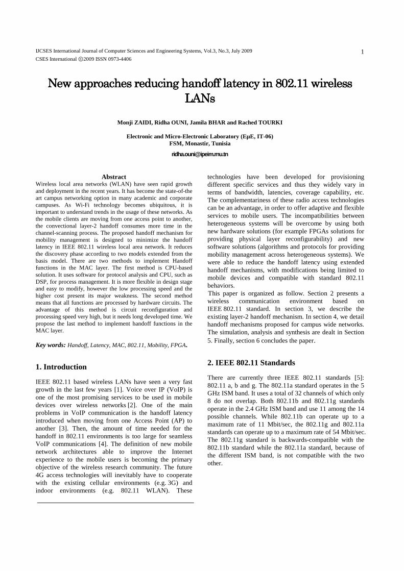
IJCSES International Journal of Computer Sciences and Engineering Systems, Vol.3, No.3, July 2009
CSES International ⓒ2009 ISSN 0973-4406
1
New approaches reducing handoff latency in 802.11 wireless New approaches reducing handoff latency in 802.11 wireless New approaches reducing handoff latency in 802.11 wireless New approaches reducing handoff latency in 802.11 wireless
LANsLANsLANsLANs
Monji ZAIDI, Ridha OUNI, Jamila BHAR and Rached TOU RKI
Electronic and Micro-Electronic Laboratory (EµE, IT -06) FSM, Monastir, Tunisia
Abstract Wireless local area networks (WLAN) have seen rapid growth and deployment in the recent years. It has become the state-of-the art campus networking option in many academic and corporate campuses. As Wi-Fi technology becomes ubiquitous, it is important to understand trends in the usage of these networks. As the mobile clients are moving from one access point to another, the convectional layer-2 handoff consumes more time in the channel-scanning process. The proposed handoff mechanism for mobility management is designed to minimize the handoff latency in IEEE 802.11 wireless local area network. It reduces the discovery phase according to two models extended from the basis model. There are two methods to implement Handoff functions in the MAC layer. The first method is CPU-based solution. It uses software for protocol analysis and CPU, such as DSP, for process management. It is more flexible in design stage and easy to modify, however the low processing speed and the higher cost present its major weakness. The second method means that all functions are processed by hardware circuits. The advantage of this method is circuit reconfiguration and processing speed very high, but it needs long developed time. We propose the last method to implement handoff functions in the MAC layer. Key words: Handoff, Latency, MAC, 802.11, Mobility, FPGA.
1. Introduction
IEEE 802.11 based wireless LANs have seen a very fast growth in the last few years [1]. Voice over IP (VoIP) is one of the most promising services to be used in mobile devices over wireless networks [2]. One of the main problems in VoIP communication is the handoff latency introduced when moving from one Access Point (AP) to another [3]. Then, the amount of time needed for the handoff in 802.11 environments is too large for seamless VoIP communications [4]. The definition of new mobile network architectures able to improve the Internet experience to the mobile users is becoming the primary objective of the wireless research community. The future 4G access technologies will inevitably have to cooperate with the existing cellular environments (e.g. 3G) and indoor environments (e.g. 802.11 WLAN). These
technologies have been developed for provisioning different specific services and thus they widely vary in terms of bandwidth, latencies, coverage capability, etc. The complementariness of these radio access technologies can be an advantage, in order to offer adaptive and flexible services to mobile users. The incompatibilities between heterogeneous systems will be overcome by using both new hardware solutions (for example FPGAs solutions for providing physical layer reconfigurability) and new software solutions (algorithms and protocols for providing mobility management across heterogeneous systems). We were able to reduce the handoff latency using extended handoff mechanisms, with modifications being limited to mobile devices and compatible with standard 802.11 behaviors.
This paper is organized as follow. Section 2 presents a wireless communication environment based on IEEE 802.11 standard. In section 3, we describe the existing layer-2 handoff mechanism. In section 4, we detail handoff mechanisms proposed for campus wide networks. The simulation, analysis and synthesis are dealt in Section 5. Finally, section 6 concludes the paper.
2. IEEE 802.11 Standards
There are currently three IEEE 802.11 standards [5]: 802.11 a, b and g. The 802.11a standard operates in the 5 GHz ISM band. It uses a total of 32 channels of which only 8 do not overlap. Both 802.11b and 802.11g standards operate in the 2.4 GHz ISM band and use 11 among the 14 possible channels. While 802.11b can operate up to a maximum rate of 11 Mbit/sec, the 802.11g and 802.11a standards can operate up to a maximum rate of 54 Mbit/sec. The 802.11g standard is backwards-compatible with the 802.11b standard while the 802.11a standard, because of the different ISM band, is not compatible with the two other.
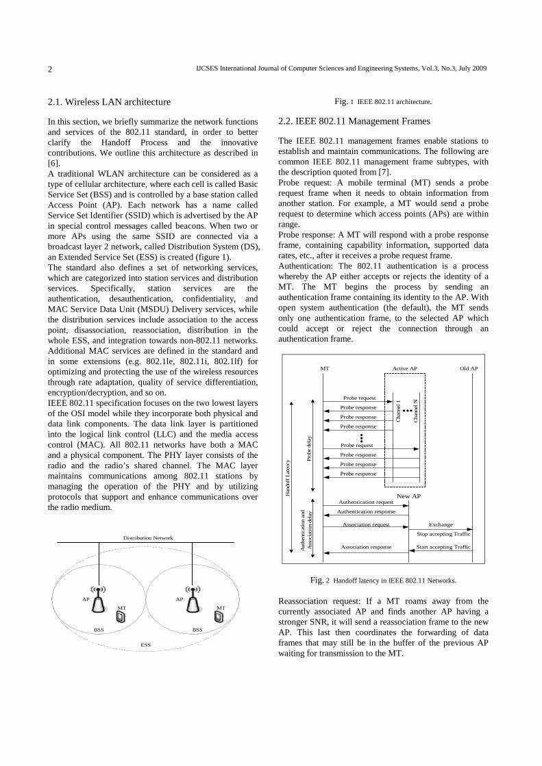
IJCSES International Journal of Computer Sciences and Engineering Systems, Vol.3, No.3, July 2009
2
2.1. Wireless LAN architecture
In this section, we briefly summarize the network functions and services of the 802.11 standard, in order to better clarify the Handoff Process and the innovative contributions. We outline this architecture as described in [6]. A traditional WLAN architecture can be considered as a type of cellular architecture, where each cell is called Basic Service Set (BSS) and is controlled by a base station called Access Point (AP). Each network has a name called Service Set Identifier (SSID) which is advertised by the AP in special control messages called beacons. When two or more APs using the same SSID are connected via a broadcast layer 2 network, called Distribution System (DS), an Extended Service Set (ESS) is created (figure 1). The standard also defines a set of networking services, which are categorized into station services and distribution services. Specifically, station services are the authentication, desauthentication, confidentiality, and MAC Service Data Unit (MSDU) Delivery services, while the distribution services include association to the access point, disassociation, reassociation, distribution in the whole ESS, and integration towards non-802.11 networks. Additional MAC services are defined in the standard and in some extensions (e.g. 802.1le, 802.11i, 802.1lf) for optimizing and protecting the use of the wireless resources through rate adaptation, quality of service differentiation, encryption/decryption, and so on. IEEE 802.11 specification focuses on the two lowest layers of the OSI model while they incorporate both physical and data link components. The data link layer is partitioned into the logical link control (LLC) and the media access control (MAC). All 802.11 networks have both a MAC and a physical component. The PHY layer consists of the radio and the radio’s shared channel. The MAC layer maintains communications among 802.11 stations by managing the operation of the PHY and by utilizing protocols that support and enhance communications over the radio medium.
ESS
BSS BSS
Distribution Network
AP AP
MT MT
Fig. 1 IEEE 802.11 architecture.
2.2. IEEE 802.11 Management Frames
The IEEE 802.11 management frames enable stations to establish and maintain communications. The following are common IEEE 802.11 management frame subtypes, with the description quoted from [7]. Probe request: A mobile terminal (MT) sends a probe request frame when it needs to obtain information from another station. For example, a MT would send a probe request to determine which access points (APs) are within range. Probe response: A MT will respond with a probe response frame, containing capability information, supported data rates, etc., after it receives a probe request frame. Authentication: The 802.11 authentication is a process whereby the AP either accepts or rejects the identity of a MT. The MT begins the process by sending an authentication frame containing its identity to the AP. With open system authentication (the default), the MT sends only one authentication frame, to the selected AP which could accept or reject the connection through an authentication frame.
MT Active AP Old AP
New AP
Probe request
Probe response
Probe response
Probe response
Probe request
Probe response
Probe response
Probe response
...
...
Chann
el 1
Cha
nnel N
Authentication request
Authentication response
Association request
Association response
Exchange
Stop accepting Traffic
Start accepting Traffic
Hand
off La
tency P
robe
dela
yA
uth
ent
icatio
n a
nd
Ass
oci
atio
n d
ela
y
Fig. 2 Handoff latency in IEEE 802.11 Networks.
Reassociation request: If a MT roams away from the currently associated AP and finds another AP having a stronger SNR, it will send a reassociation frame to the new AP. This last then coordinates the forwarding of data frames that may still be in the buffer of the previous AP waiting for transmission to the MT.
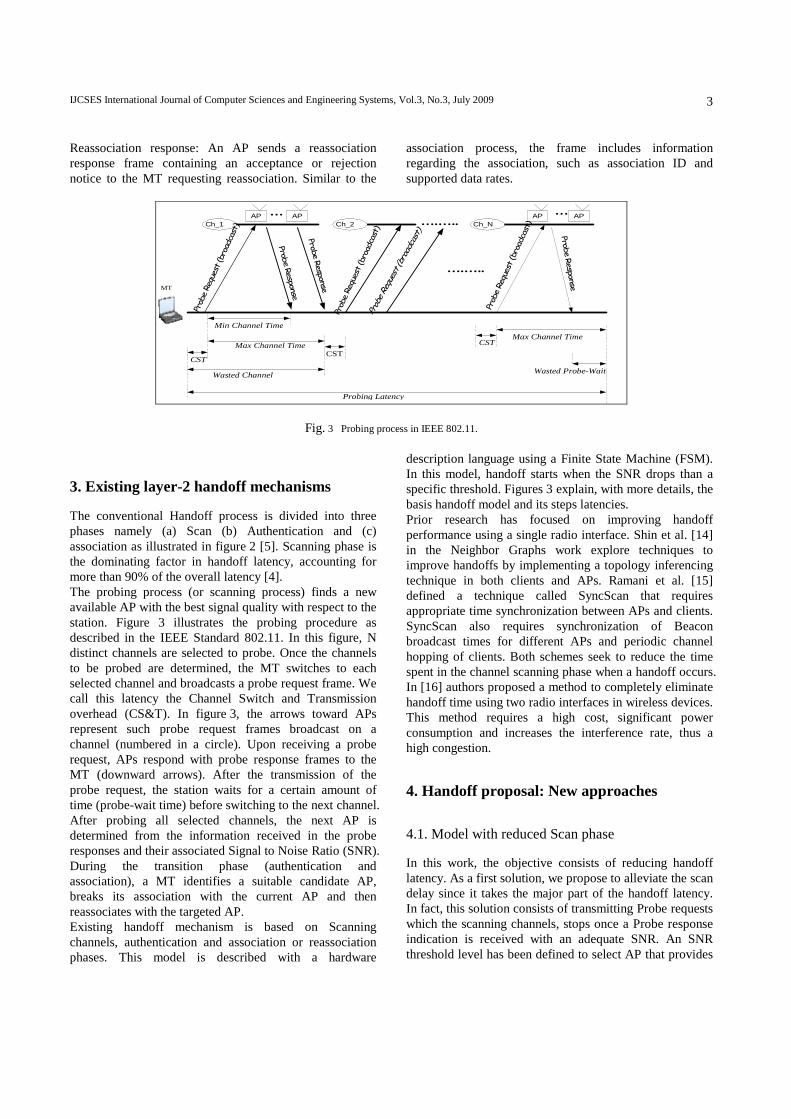
IJCSES International Journal of Computer Sciences and Engineering Systems, Vol.3, No.3, July 2009
3
Reassociation response: An AP sends a reassociation response frame containing an acceptance or rejection notice to the MT requesting reassociation. Similar to the
association process, the frame includes information regarding the association, such as association ID and supported data rates.
AP AP APCh_1 Ch_NCh_2
Probe Request (broadcast)
Probe R
esponse
Probe R
esponse
Probe Request (broadcast)
Probe Request (broadcast)
Probe Request (broadcast)
Probe R
esponse
Probing Latency
….…..
….…..
…
Min Channel Time
Max Channel Time CST
CST
CST
Wasted Channel
Max Channel Time
Wasted Probe-Wait
MT
AP…
Fig. 3 Probing process in IEEE 802.11.
3. Existing layer-2 handoff mechanisms
The conventional Handoff process is divided into three phases namely (a) Scan (b) Authentication and (c) association as illustrated in figure 2 [5]. Scanning phase is the dominating factor in handoff latency, accounting for more than 90% of the overall latency [4]. The probing process (or scanning process) finds a new available AP with the best signal quality with respect to the station. Figure 3 illustrates the probing procedure as described in the IEEE Standard 802.11. In this figure, N distinct channels are selected to probe. Once the channels to be probed are determined, the MT switches to each selected channel and broadcasts a probe request frame. We call this latency the Channel Switch and Transmission overhead (CS&T). In figure 3, the arrows toward APs represent such probe request frames broadcast on a channel (numbered in a circle). Upon receiving a probe request, APs respond with probe response frames to the MT (downward arrows). After the transmission of the probe request, the station waits for a certain amount of time (probe-wait time) before switching to the next channel. After probing all selected channels, the next AP is determined from the information received in the probe responses and their associated Signal to Noise Ratio (SNR). During the transition phase (authentication and association), a MT identifies a suitable candidate AP, breaks its association with the current AP and then reassociates with the targeted AP. Existing handoff mechanism is based on Scanning channels, authentication and association or reassociation phases. This model is described with a hardware
description language using a Finite State Machine (FSM). In this model, handoff starts when the SNR drops than a specific threshold. Figures 3 explain, with more details, the basis handoff model and its steps latencies. Prior research has focused on improving handoff performance using a single radio interface. Shin et al. [14] in the Neighbor Graphs work explore techniques to improve handoffs by implementing a topology inferencing technique in both clients and APs. Ramani et al. [15] defined a technique called SyncScan that requires appropriate time synchronization between APs and clients. SyncScan also requires synchronization of Beacon broadcast times for different APs and periodic channel hopping of clients. Both schemes seek to reduce the time spent in the channel scanning phase when a handoff occurs. In [16] authors proposed a method to completely eliminate handoff time using two radio interfaces in wireless devices. This method requires a high cost, significant power consumption and increases the interference rate, thus a high congestion.
4. Handoff proposal: New approaches
4.1. Model with reduced Scan phase
In this work, the objective consists of reducing handoff latency. As a first solution, we propose to alleviate the scan delay since it takes the major part of the handoff latency. In fact, this solution consists of transmitting Probe requests which the scanning channels, stops once a Probe response indication is received with an adequate SNR. An SNR threshold level has been defined to select AP that provides
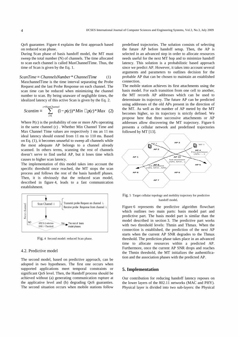
IJCSES International Journal of Computer Sciences and Engineering Systems, Vol.3, No.3, July 2009
4
QoS guarantee. Figure 4 explains the first approach based on reduced scan phase. During Scan phase of basis handoff model, the MT must sweep the total number (N) of channels. The time allocated to scan each channel is called MaxChannelTime. Thus, the time of Scan is given by the Eq. 1.
eChannelTim*mberChannelsNuScanTime = (1) MaxchannelTime is the time interval separating the Probe Request and the last Probe Response on each channel. The scan time can be reduced when minimizing the channel number to scan. By being unaware of negligible times, the idealized latency of this active Scan is given by the Eq. 2.
)2(*)(*))(1(1∑
=
=
+−=NumChannelc
c
MaxcpMincpScantim
Where P(c) is the probability of one or more APs operating in the same channel (c) . Whether Min Channel Time and Max Channel Time values are respectively 1 ms an 11 ms ideal latency should extend from 11 ms to 110 ms. Based on Eq. (1), it becomes unuseful to sweep all channels while the most adequate AP belongs to a channel already scanned. In others terms, scanning the rest of channels doesn’t serve to find useful AP, but it loses time which causes to higher scan latency. The implementation of this model takes into account the specific threshold once reached, the MT stops the scan process and follows the rest of the basis handoff phases. Then, it is obviously that the reduced scan model, described in figure 4, leads to a fast communication establishment.
Scan Channel i
AP(Ch i) selectionSNR i >Thershold
The rest of basismodel phases
Nex
t ch
anne
l
Transmit probe Request on channel i.Receive probe Response from channel i.
YesNO
Fig. 4 Second model: reduced Scan phase.
4.2. Predictive model
The second model, based on predictive approach, can be adopted in two hypotheses. The first one occurs when supported applications meet temporal constraints or significant QoS level. Then, the Handoff process should be achieved without (a) generating communication rupture at the applicative level and (b) degrading QoS guaranties. The second situation occurs when mobile stations follow
predefined trajectories. The solution consists of selecting the future AP before handoff setup. Then, the AP is selected in an advanced step in order to allocate resources needs useful for the next MT hop and to minimize handoff latency. This solution is a probabilistic based approach since we predict AP. However, it takes into account several arguments and parameters to outlines decision for the probable AP that can be chosen to maintain an established connection. The mobile station achieves its first attachments using the basis model. For each transition from one cell to another, the MT records AP addresses which can be used to determinate its trajectory. The future AP can be predicted using addresses of the old APs present in the direction of the MT. As well as the number of AP meted by the MT becomes higher, so its trajectory is strictly defined. We propose here that three successive attachments or AP addresses allow discovering the MT trajectory. Figure 6 presents a cellular network and predefined trajectories followed by MT [13].
AP 4
AP 10
AP 5
AP 6
AP 2
AP 9
AP 1
AP 7
AP 8
AP 3
First attachment(AP4, - , -)
Snd attachment(AP4, AP10 , -)
3rd attachment(AP4, AP10 , AP9)
MT 1MT 2
Fig. 5 Target cellular topology and mobility trajectory for predictive
handoff model.
Figure 6 represents the predictive algorithm flowchart which outlines two main parts: basis model part and predictive part. The basis model part is similar than the model described in section 3. The predictive part works with two threshold levels: Thmin and Thmax. When the connection is established, the prediction of the next AP starts when the current AP SNR degrades to the Thmax threshold. The prediction phase takes place in an advanced time to allocate resources within a predicted AP. Furthermore, once the current AP SNR drops and reaches the Thmin threshold, the MT initializes the authentifica-tion and the association phases with the predicted AP.
5. Implementation
Our contribution for reducing handoff latency reposes on the lower layers of the 802.11 networks (MAC and PHY). Physical layer is divided into two sub-layers: the Physical
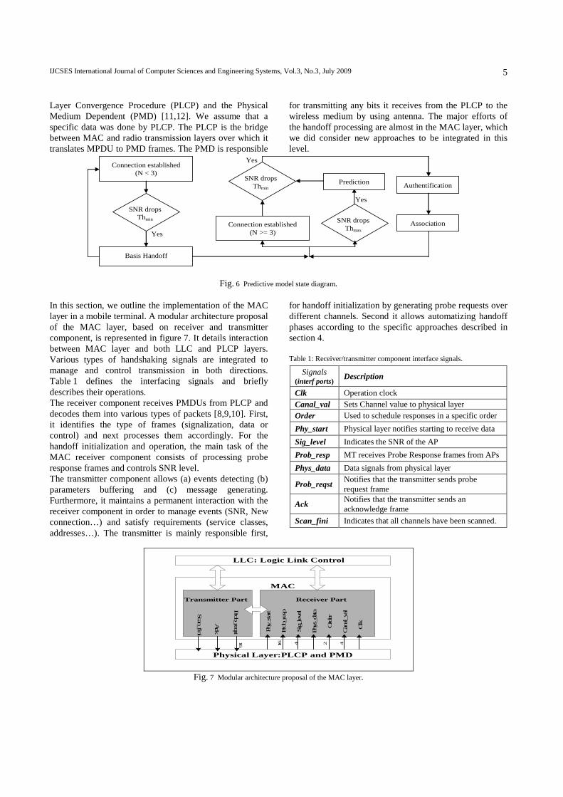
IJCSES International Journal of Computer Sciences and Engineering Systems, Vol.3, No.3, July 2009
5
Layer Convergence Procedure (PLCP) and the Physical Medium Dependent (PMD) [11,12]. We assume that a specific data was done by PLCP. The PLCP is the bridge between MAC and radio transmission layers over which it translates MPDU to PMD frames. The PMD is responsible
for transmitting any bits it receives from the PLCP to the wireless medium by using antenna. The major efforts of the handoff processing are almost in the MAC layer, which we did consider new approaches to be integrated in this level.
Connection established
(N < 3)
SNR drops Thmin
Basis Handoff
Connection established (N >= 3)
SNR drops Thmin
SNR drops Thmax
Prediction Authentification
Association
Yes
Yes
Yes
Fig. 6 Predictive model state diagram.
In this section, we outline the implementation of the MAC layer in a mobile terminal. A modular architecture proposal of the MAC layer, based on receiver and transmitter component, is represented in figure 7. It details interaction between MAC layer and both LLC and PLCP layers. Various types of handshaking signals are integrated to manage and control transmission in both directions. Table 1 defines the interfacing signals and briefly describes their operations. The receiver component receives PMDUs from PLCP and decodes them into various types of packets [8,9,10]. First, it identifies the type of frames (signalization, data or control) and next processes them accordingly. For the handoff initialization and operation, the main task of the MAC receiver component consists of processing probe response frames and controls SNR level. The transmitter component allows (a) events detecting (b) parameters buffering and (c) message generating. Furthermore, it maintains a permanent interaction with the receiver component in order to manage events (SNR, New connection…) and satisfy requirements (service classes, addresses…). The transmitter is mainly responsible first,
for handoff initialization by generating probe requests over different channels. Second it allows automatizing handoff phases according to the specific approaches described in section 4.
Table 1: Receiver/transmitter component interface signals.
Signals (interf ports) Description
Clk Operation clock Canal_val Sets Channel value to physical layer Order Used to schedule responses in a specific order
Phy_start Physical layer notifies starting to receive data
Sig_level Indicates the SNR of the AP
Prob_resp MT receives Probe Response frames from APs
Phys_data Data signals from physical layer
Prob_reqst Notifies that the transmitter sends probe request frame
Ack Notifies that the transmitter sends an acknowledge frame
Scan_fini Indicates that all channels have been scanned.
Phy_
start
Pro
b_re
sp
Sig_leve
l
Phys
_dataP
rob_re
qst
Ack
Canal_va
l
OrderS
can_fin
i
Physical Layer:PLCP and PMD
MAC
LLC: Logic Link Control
Clk
Transmitter Part Receiver Part
16 4 2 4
16
Fig. 7 Modular architecture proposal of the MAC layer.
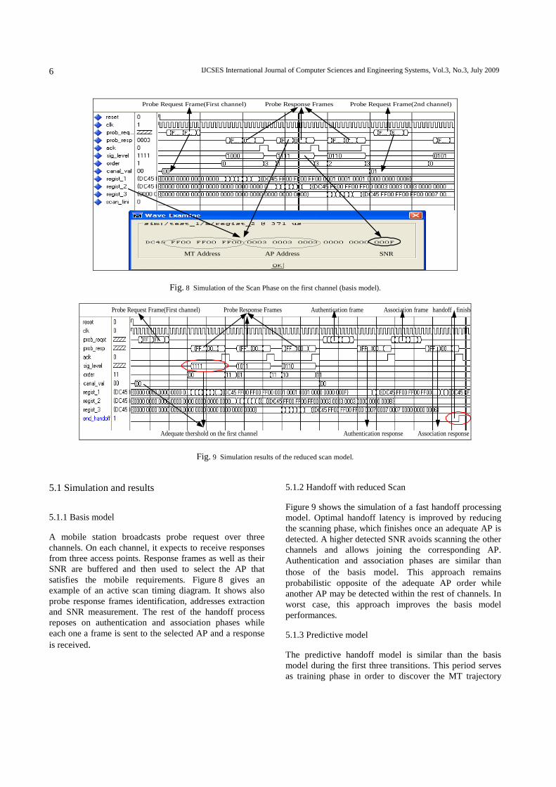
IJCSES International Journal of Computer Sciences and Engineering Systems, Vol.3, No.3, July 2009
6
Probe Response FramesProbe Request Frame(First channel)
MT Address AP Address SNR
Probe Request Frame(2nd channel)
Fig. 8 Simulation of the Scan Phase on the first channel (basis model).
Probe Request Frame(First channel) Probe Response Frames Authentication frame Association frame
Association responseAdequate thershold on the first channel Authentication response
handoff finished
Fig. 9 Simulation results of the reduced scan model.
5.1 Simulation and results
5.1.1 Basis model
A mobile station broadcasts probe request over three channels. On each channel, it expects to receive responses from three access points. Response frames as well as their SNR are buffered and then used to select the AP that satisfies the mobile requirements. Figure 8 gives an example of an active scan timing diagram. It shows also probe response frames identification, addresses extraction and SNR measurement. The rest of the handoff process reposes on authentication and association phases while each one a frame is sent to the selected AP and a response is received.
5.1.2 Handoff with reduced Scan
Figure 9 shows the simulation of a fast handoff processing model. Optimal handoff latency is improved by reducing the scanning phase, which finishes once an adequate AP is detected. A higher detected SNR avoids scanning the other channels and allows joining the corresponding AP. Authentication and association phases are similar than those of the basis model. This approach remains probabilistic opposite of the adequate AP order while another AP may be detected within the rest of channels. In worst case, this approach improves the basis model performances.
5.1.3 Predictive model
The predictive handoff model is similar than the basis model during the first three transitions. This period serves as training phase in order to discover the MT trajectory
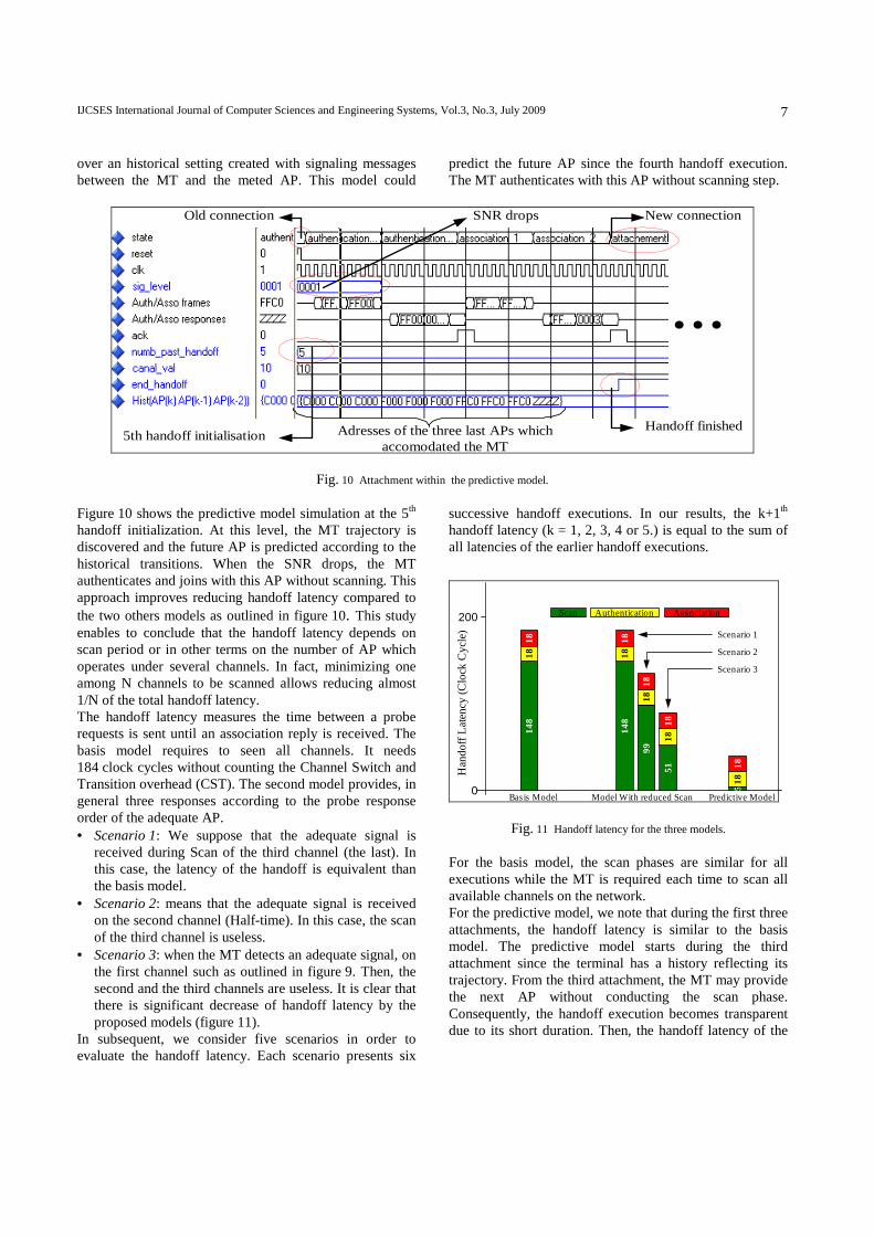
IJCSES International Journal of Computer Sciences and Engineering Systems, Vol.3, No.3, July 2009
7
over an historical setting created with signaling messages between the MT and the meted AP. This model could
predict the future AP since the fourth handoff execution. The MT authenticates with this AP without scanning step.
SNR drops
5th handoff initialisation
Adresses of the three last APs whichaccomodated the MT
Old connection New connection
Handoff finished
...
Fig. 10 Attachment within the predictive model.
Figure 10 shows the predictive model simulation at the 5th handoff initialization. At this level, the MT trajectory is discovered and the future AP is predicted according to the historical transitions. When the SNR drops, the MT authenticates and joins with this AP without scanning. This approach improves reducing handoff latency compared to the two others models as outlined in figure 10. This study enables to conclude that the handoff latency depends on scan period or in other terms on the number of AP which operates under several channels. In fact, minimizing one among N channels to be scanned allows reducing almost 1/N of the total handoff latency. The handoff latency measures the time between a probe requests is sent until an association reply is received. The basis model requires to seen all channels. It needs 184 clock cycles without counting the Channel Switch and Transition overhead (CST). The second model provides, in general three responses according to the probe response order of the adequate AP. • Scenario 1: We suppose that the adequate signal is
received during Scan of the third channel (the last). In this case, the latency of the handoff is equivalent than the basis model.
• Scenario 2: means that the adequate signal is received on the second channel (Half-time). In this case, the scan of the third channel is useless.
• Scenario 3: when the MT detects an adequate signal, on the first channel such as outlined in figure 9. Then, the second and the third channels are useless. It is clear that there is significant decrease of handoff latency by the proposed models (figure 11).
In subsequent, we consider five scenarios in order to evaluate the handoff latency. Each scenario presents six
successive handoff executions. In our results, the k+1th handoff latency (k = 1, 2, 3, 4 or 5.) is equal to the sum of all latencies of the earlier handoff executions.
18
14
81
8
18
99
18
18
51
18
18
14
81
8Scan AssociationAuthentication
18
51
8
Basis Model Model With reduced Scan Predictive Model
Han
do
ff L
aten
cy (
Clo
ck C
ycle
)
0
200Scenario 1
Scenario 2
Scenario 3
Fig. 11 Handoff latency for the three models.
For the basis model, the scan phases are similar for all executions while the MT is required each time to scan all available channels on the network. For the predictive model, we note that during the first three attachments, the handoff latency is similar to the basis model. The predictive model starts during the third attachment since the terminal has a history reflecting its trajectory. From the third attachment, the MT may provide the next AP without conducting the scan phase. Consequently, the handoff execution becomes transparent due to its short duration. Then, the handoff latency of the
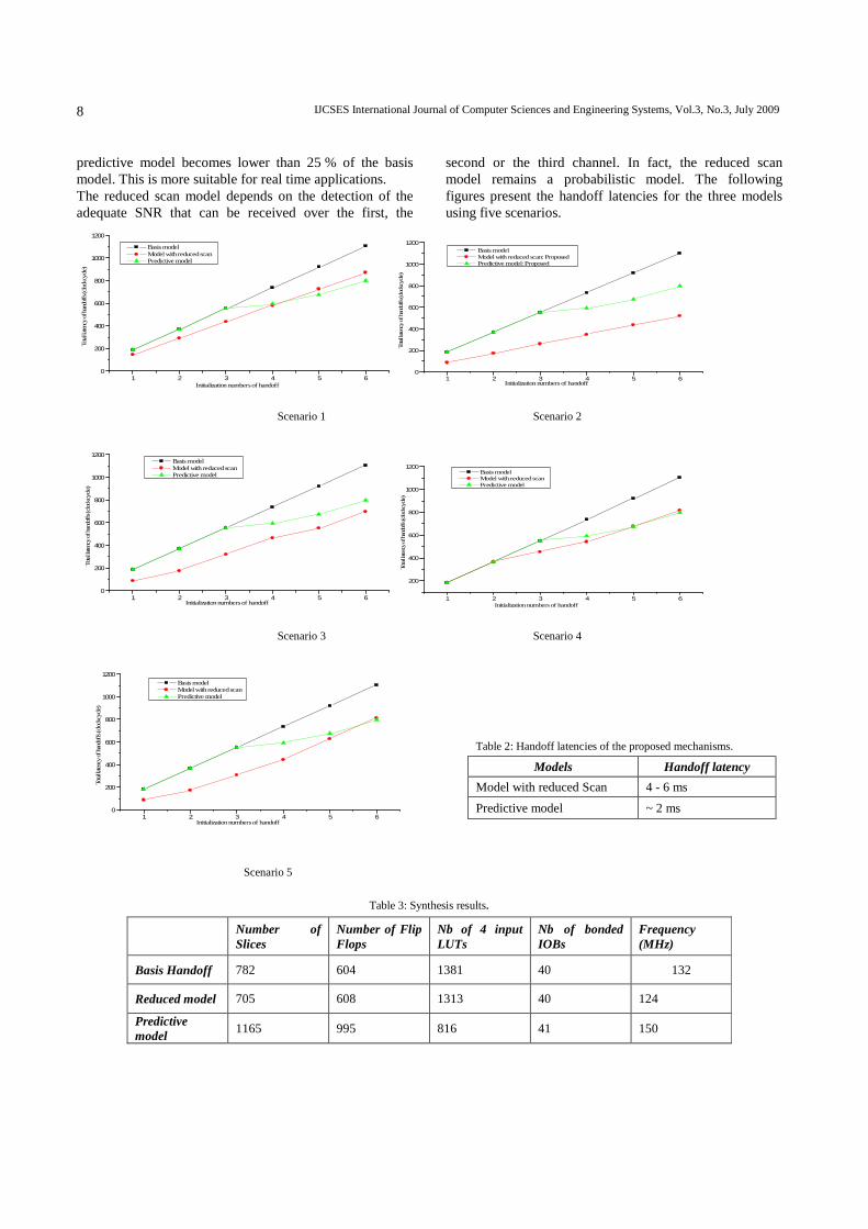
IJCSES International Journal of Computer Sciences and Engineering Systems, Vol.3, No.3, July 2009
8
predictive model becomes lower than 25 % of the basis model. This is more suitable for real time applications. The reduced scan model depends on the detection of the adequate SNR that can be received over the first, the
second or the third channel. In fact, the reduced scan model remains a probabilistic model. The following figures present the handoff latencies for the three models using five scenarios.
1 2 3 4 5 60
200
400
600
800
1000
1200
Basis model Model with reduced scan Predictive model
Tota
l late
ncy
of h
ando
ffs (cloc
k cy
cle)
Initialization numbers of handoff 1 2 3 4 5 6
0
200
400
600
800
1000
1200 Basis model Model with reduced scan: Proposed Predictive model: Proposed
Tota
l latenc
y of han
doffs
(clock
cyc
le)
Initialization numbers of handoff
Scenario 1 Scenario 2
1 2 3 4 5 60
200
400
600
800
1000
1200 Basis model Model with reduced scan Predictive model
Tota
l late
ncy
of h
ando
ffs (cloc
k cyc
le)
Initialization numbers of handoff 1 2 3 4 5 6
200
400
600
800
1000
1200 Basis model Model with reduced scan Predictive model
Tota
l latenc
y of hand
offs (c
lock
cyc
le)
Initialization numbers of handoff
Scenario 3 Scenario 4
1 2 3 4 5 6
0
200
400
600
800
1000
1200 Basis model Model with reduced scan Predictive model
Tota
l late
ncy
of han
doffs
(clock
cyc
le)
Initialization numbers of handoff
Scenario 5
Table 2: Handoff latencies of the proposed mechanisms.
Models Handoff latency
Model with reduced Scan 4 - 6 ms
Predictive model ~ 2 ms
Table 3: Synthesis results.
Number of Slices
Number of Flip Flops
Nb of 4 input LUTs
Nb of bonded IOBs
Frequency (MHz)
Basis Handoff 782 604 1381 40 132
Reduced model 705 608 1313 40 124
Predictive model
1165 995 816 41 150
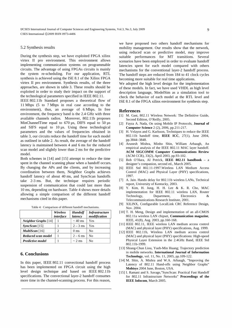
IJCSES International Journal of Computer Sciences and Engineering Systems, Vol.3, No.3, July 2009
CSES International ⓒ2009 ISSN 0973-4406
9
5.2 Synthesis results
During the synthesis step, we have exploited FPGA xilinx virtex II pro environment. This environment allows implementing communication systems on programmable circuits. The advantage of using FPGAs circuits is mainly the system re-scheduling. For our application, RTL synthesis is achieved using the ISE 8.1 of the Xilinx FPGA virtex II pro environment. Synthesis results, of the three approaches, are shown in table 3. These results should be exploited in order to study their impact on the support of the technological parameters specified in IEEE 802.11. IEEE 802.11b Standard proposes a theoretical flow of 11 Mbps (5 to 7 Mbps in real case according to the environment), thus, an average of 6 Mbps. In free environment, the frequency band is the 2.4 GHz with three available channels radios. Moreover, 802.11b proposes MinChannelTime equal to 670 µs, DIFS equal to 50 µs and SIFS equal to 10 µs. Using these technological parameters and the values of frequencies obtained in table 3, our circuits reduce the handoff time for each model as outlined in table 2. As result, the average of the handoff latency is maintained between 4 and 6 ms for the reduced scan model and slightly lower than 2 ms for the predictive model. Both schemes in [14] and [15] attempt to reduce the time spent in the channel scanning phase when a handoff occurs. By changing the APs and the clients, and by increasing coordination between them, Neighbor Graphs achieves handoff latency of about 40 ms, and SyncScan handoffs take 2-3 ms. But, the technique requires periodic suspension of communication that could last more than 10 ms, depending on hardware. Table 4 shows more details allowing a simple comparison of the different handoff mechanisms cited in this paper.
Table 4: Comparison of different handoff mechanisms.
Wireless interface
Handoff latency
Infrastructure modification
Neighbor Graphs [14] 1 ~ 40 ms Yes
SyncScan [15] 1 2 – 3 ms Yes
MultiScan [16] 2 0 ms No
Reduced scan model 1 2 – 6 ms No
Predictive model 1 ~ 2 ms No
6. Conclusions
In this paper, IEEE 802.11 convectional handoff process has been implemented on FPGA circuit using the high level design technique and based on IEEE 802.11b specifications. The convectional layer-2 handoff consumes more time in the channel-scanning process. For this reason,
we have proposed two others handoff mechanisms for mobility management. Our results show that the network, using reduced scan or predictive model, may improve suitable performances for MT transitions. Several scenarios have been employed in order to evaluate handoff latencies spent for each model compared with others mechanisms for the conventional layer-2 handoff process. The handoff steps are reduced from 184 to 41 clock cycles becoming more suitable for real time applications. We adopted the high level design for the implementation of these models. In fact, we have used VHDL as high level description language, ModelSim as a simulation tool to check the behavior of each model at the RTL level and ISE 8.1 of the FPGA xilinx environment for synthesis step.
References [1] M. Gast, 802.11 Wireless Network: The Definitive Guide,
Second Edition, O’Reilly, 2005. [2] Fayza A. Nada, On using Mobile IP Protocols, Journal of
Computer Science 2 (2), 2006, pp.211-217. [3] H. Velayos and G. Karlsson, Techniques to reduce the IEEE
802.11b handoff time, IEEE ICC , 27(1), June 2004, pp.3844–3848.
[4] Arunesh Mishra, Minho Shin, William Arbaugh, An empirical analysis of the IEEE 802.11 MAC layer handoff. ACM SIGCOMM Computer Communications Review (ACM CCR), 33(2), April 2003, pp.93-102.
[5] Bob O’Hara, AI Petrick, IEEE 802.11 handbook – a designer’s companion, second ed., March 2005.
[6] IEEE Std 802.11-1997.Wireless LAN Medium Access Control (MAC) and Physical Layer (PHY) specifications, 1997.
[7] A. Jain. Hando delay for 802.11b wireless LANs, Technical report, University of Kentucky, 2003.
[8] Y. Kim, H. Jung, H. H. Lee & K. R. Cho, MAC implementation for IEEE 802.11 wireless LAN, Router Technology, Department, Electronics & Telecommunications Research Institute, 2001.
[9] XILINX, Configurable LocalLink CRC Reference Design, Nov. 2004.
[10] T. H. Meng, Design and implementation of an all-CMOS 802.11a wireless LAN chipset, Communication magazine, IEEE, 41(8), Aug. 2003, pp.160-168.
[11] IEEE 802.11, IEEE wireless LAN medium access control (MAC) and physical layer (PHY) specifications, Aug. 1999.
[12] IEEE 802.11b, Wireless LAN medium access control (MAC) and physical layer (PHY) specifications: High-speed Physical Layer Extension in the 2.4GHz Band, IEEE Std 802.11b-1999.
[13] Shiang-Chun Liou, Yueh-Min Huang; Trajectory prediction in mobile networks. International Journal of Information Technology, vol. 11, No. 11, 2005, pp.109-122.
[14] M. Shin, A. Mishra and W.A. Arbaugh, ”Improving the Latency of 802.11 Hand-offs using Neighbor Graphs” Mobisys 2004 June, Boston, USA.
[15] I. Ramani and S. Savage,”SyncScan: Practical Fast Handoff for 802.11 Infrastructure Networks” Proceedings of the IEEE Infocom, March 2005.
IJCSES International Journal of Computer Sciences and Engineering Systems, Vol.3, No.3, July 2009
10
[16] Vladimir Brik, Arunesh Mishra, Suman Banerjee, Eliminating handoff latencies in 802.11 WLANs using Multiple Radios, Applications, Experience, and Evaluation, Internet Measurment Conference 2005: 299-304.
International Journal of Computers, Systems and Signals, Vol. 10, No.1, 2009 27
LOW POWER ASIC DESIGNS FOR FAST HANDOFF IN
IEEE802.11
Monji Zaidi, Ridha Ouni, Kholdoun Torki and Rached Tourki
Electronic and Micro-Electronic Laboratory (EµE, IT-06)
FSM, Monastir, Tunisia
CPM, 46, Avenue Felix VIALLAET 38031 GRENOBLE cedex, France
E-mail: [email protected]
ABSTRACT The Handoff process is a key problem in many wireless network processing applications. Current
implementations of this process using software implementation are time consuming and cannot
meet the gigabit bandwidth requirements. Implementing this process within the hardware
improves the search time considerably and has several other advantages like reducing power
consumption. In this paper we present an array based hardware implementation of this time consuming process for network mobility. A new mechanism for mobility management to
minimize the handoff latency in IEEE 802.11 wireless local area network is also presented.
Compared to the basis model and at 1GHz, this new mechanism allows a profit of 60% in power
consumption and 20% in silicon area. Those two designs are described in VHDL at the RTL level
language and implemented on an ASIC (Application-Specific Integrated Circuit) and are evaluated
in terms of speed, area and power consumption.
Keywords: IEEE 802.11, Handoff, MAC, design, ASIC
1. INTRODUCTION
The world of WLANs is truly an exciting area, with major activity worldwide,
challenging traditional service providers and business models. Initially, WLANs were meant to be
an augmentation, not a replacement, of wired LANs and premises telephone systems. WLANs
were deployed in enterprise or corporate locations where there might be a number of factors that
limited or prevented wired systems from being installed. Today, we see much greater utility for
WLANs, as evidenced by the emergence of thousands of hotspots around the world. In some
cases, it is cheaper to deploy wireless in an office than to replace a crumbling old token-ring cable
plant with shiny new Ethernet. In general, WLANs operate over short ranges, anywhere from 10 to
500 feet (3 to 150 m), so their coverage areas are microcells or piccocells.
Mobility is the most important feature of a WLANs system. Undoubtedly the future perspective of networking will demand to support mobile users traveling all over the world. In
addition to that, the number of portable devices that need access to the Internet is exponentially
increasing. Users on the other hand are no longer required to work in their company's home
network while they may be moving from place to place. Usually, continuous service is achieved
by supporting handover from one cell to another. Handover is the process of changing the channel
(frequency, time slot, spreading code, or combination of them) associated with the current
connection while a communication is in progress. It is often initiated either by crossing a cell
boundary or by deterioration in quality of the signal in the current channel.
In IEEE 802.11 based wireless LAN, when the Mobile Terminal (MT) changes its point
of attachment to the internet, it may produce a service interruption, since the MT cannot send or
receive any packets from the time at which it disconnects from one point of attachment to the time
ISSN 1608-5655 (Online), Category: Research articles, Publisher: IAAMSAD
28 International Journal of Computers, Systems and Signals, Vol. 10, No.1, 2009
at which it registers with a new point of attachment. Such an interruption would be unacceptable
for real time services such as voice-over IP, which demands a further optimization of the mobility
management in IEEE 802.11 based WLAN. Our motivation is to study the impact of the handoffs
for delay of the sensitive applications. Our evaluation results show that the conventional handover
is not totally effective for QoS requirements. So, we propose a hardware implementation for the
handoff process in WLAN networks, using an ASIC circuit. The paper will be organized as follows: in section 2, an overview of related works is
provided. Section 3 presents an environment with a wireless communication based on
IEEE 802.11 standard. In section 4, we describe the existing layer-2 handoff mechanism.
Section 5, highlights the hardware implementation of handoff mechanisms (basis and proposed)
for campus wide networks. Results are dealt in Section 6. Finally, section 7 is the concluding part
of the paper.
2. RELATED WORKS
The literature contains several efforts proposing a mobility modeling and management
approaches aiming at improving the handoff management and at optimizing resource reservations.
In (Choi C.H. et. al., 2002), the authors suggest the use of an adaptive bandwidth reservation based on a mobility graph and 2-tier cell structure to determine the amount of
bandwidth to be reserved in the cell. Another resource reservation approach is presented in (Islam
M.M. et. al., 2002) and (Islam M.M. et. al., 2003), where the authors propose a bandwidth
reservation scheme that uses a mobility parameter-based resource reservation estimator function
(RREF). This nonlinear function uses distance, direction, and velocity to calculate the probability
of a MT visiting a particular cell. The authors, in (Liu T. et. al., 1998), propose a predictive
mobility management scheme that models the MT, as a linear dynamic system driven by time
varying forcing functions that simulate subjective moving intentions from the user and objective
random perturbations from the environment. The mobility management model proposed in (Liang
B. and Haas, Z.J., 1999), is based on Gauss–Markov model where an MT’s velocity is correlated
in time to various degrees in order to predict the future location of a MT. In (Hou, J. and Fang Y., 2001), authors initiated the idea of taking the mobility into account for call admission control
algorithms. They explore many important points for mobility-based call admission control. They
indicate that it is important to make the reservation at the appropriate time to save the reserved
bandwidth.. In this model, the authors did not use the mobility history of the users to enhance the
estimation accuracy. In (Yu, F. and Leung, V.C.M., 2002), a mobility-based predictive algorithm
for call admission control was presented. This algorithm is motivated by a computational learning
theory, which has shown that prediction is synonymous with data compression. The main
limitation of this approach is that it is not applicable for a soft handoff, which makes this approach
unsuitable for most of the existing and future mobile telecommunication. Moreover, this approach
requires every adjacent Access Point (APs) to reserve the channels for all the users.
Based on the observation that the movement behaviors of the majority of people are
performed repetitively process, the author in (Tabbane, S., 1995), models the user inter-cell mobility as a time-dependent (location, probability) pair. This work uses the probability that the
user is found in a certain location during a given period of time as a base parameter. The (location,
probability) pair is derived from the long-time observation statistics. While providing a good
starting, enabling the regularity in a user’s daily movement, Tabbane’s model does not reflect an
instantaneous movement behavior, and the (location, probability) pair is not totally efficient in
representing the itineraries which are usually present in a user’s movement pattern. As a possible
solution to improve the call connectivity, the Current implementations of this process using
software methods are time consuming and cannot meet gigabit bandwidth requirements. A few
works have addressed the hardware implementation of the mobility in WLANs networks. The
authors in (Chiang, M.H, 2006), proposed a design flow system and function module of active
scan in WLANs. In (Zaidi, M et. al., 2008), we have proposed the hardware transformation and implementation of the handoff protocol from its initial software description. We have
implemented two models that reduce Scan phase during the handoff execution. These models have
been implemented on a FPGA circuit. Implementing this process in the hardware circuits
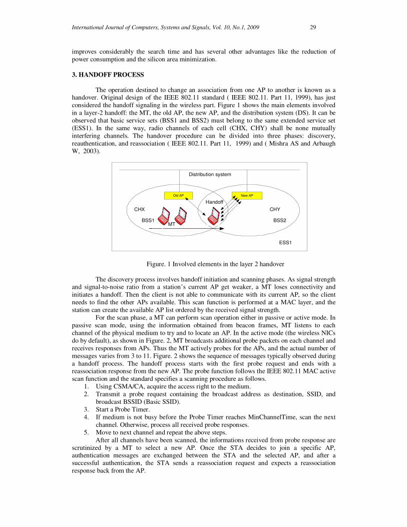
International Journal of Computers, Systems and Signals, Vol. 10, No.1, 2009 29
improves considerably the search time and has several other advantages like the reduction of
power consumption and the silicon area minimization.
3. HANDOFF PROCESS
The operation destined to change an association from one AP to another is known as a
handover. Original design of the IEEE 802.11 standard ( IEEE 802.11. Part 11, 1999), has just
considered the handoff signaling in the wireless part. Figure 1 shows the main elements involved
in a layer-2 handoff: the MT, the old AP, the new AP, and the distribution system (DS). It can be
observed that basic service sets (BSS1 and BSS2) must belong to the same extended service set
(ESS1). In the same way, radio channels of each cell (CHX, CHY) shall be none mutually
interfering channels. The handover procedure can be divided into three phases: discovery,
reauthentication, and reassociation ( IEEE 802.11. Part 11, 1999) and ( Mishra AS and Arbaugh
W, 2003).
Old AP New AP
CHX CHY
BSS1 BSS2
Handoff
ESS1
Distribution system
MT
Figure. 1 Involved elements in the layer 2 handover
The discovery process involves handoff initiation and scanning phases. As signal strength and signal-to-noise ratio from a station’s current AP get weaker, a MT loses connectivity and
initiates a handoff. Then the client is not able to communicate with its current AP, so the client
needs to find the other APs available. This scan function is performed at a MAC layer, and the
station can create the available AP list ordered by the received signal strength.
For the scan phase, a MT can perform scan operation either in passive or active mode. In
passive scan mode, using the information obtained from beacon frames, MT listens to each
channel of the physical medium to try and to locate an AP. In the active mode (the wireless NICs
do by default), as shown in Figure. 2, MT broadcasts additional probe packets on each channel and
receives responses from APs. Thus the MT actively probes for the APs, and the actual number of
messages varies from 3 to 11. Figure. 2 shows the sequence of messages typically observed during
a handoff process. The handoff process starts with the first probe request and ends with a reassociation response from the new AP. The probe function follows the IEEE 802.11 MAC active
scan function and the standard specifies a scanning procedure as follows.
1. Using CSMA/CA, acquire the access right to the medium.
2. Transmit a probe request containing the broadcast address as destination, SSID, and
broadcast BSSID (Basic SSID).
3. Start a Probe Timer.
4. If medium is not busy before the Probe Timer reaches MinChannelTime, scan the next
channel. Otherwise, process all received probe responses.
5. Move to next channel and repeat the above steps.
After all channels have been scanned, the informations received from probe response are
scrutinized by a MT to select a new AP. Once the STA decides to join a specific AP, authentication messages are exchanged between the STA and the selected AP, and after a
successful authentication, the STA sends a reassociation request and expects a reassociation
response back from the AP.
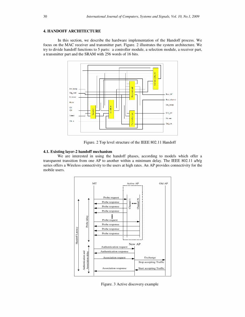
30 International Journal of Computers, Systems and Signals, Vol. 10, No.1, 2009
4. HANDOFF ARCHITECTURE
In this section, we describe the hardware implementation of the Handoff process. We
focus on the MAC receiver and transmitter part. Figure. 2 illustrates the system architecture. We
try to divide handoff functions to 5 parts: a controller module, a selection module, a receiver part,
a transmitter part and the SRAM with 256 words of 16 bits.
Figure. 2 Top level structure of the IEEE 802.11 Handoff
4.1. Existing layer-2 handoff mechanism We are interested in using the handoff phases, according to models which offer a
transparent transition from one AP to another within a minimum delay. The IEEE 802.11 a/b/g
series offers a Wireless connectivity to the users at high rates. An AP provides connectivity for the
mobile users.
MT Active AP Old AP
New AP
Probe request
Probe response
Probe response
Probe response
Probe request
Probe response
Probe response
Probe response
...
...
Channel 1
Channel N
Authentication request
Authentication response
Association request
Association response
Exchange
Stop accepting Traffic
Start accepting Traffic
Handoff
Lat
ency P
robe d
ela
y
Auth
enticati
on a
nd
Ass
oci
ati
on d
ela
y
Figure. 3 Active discovery example
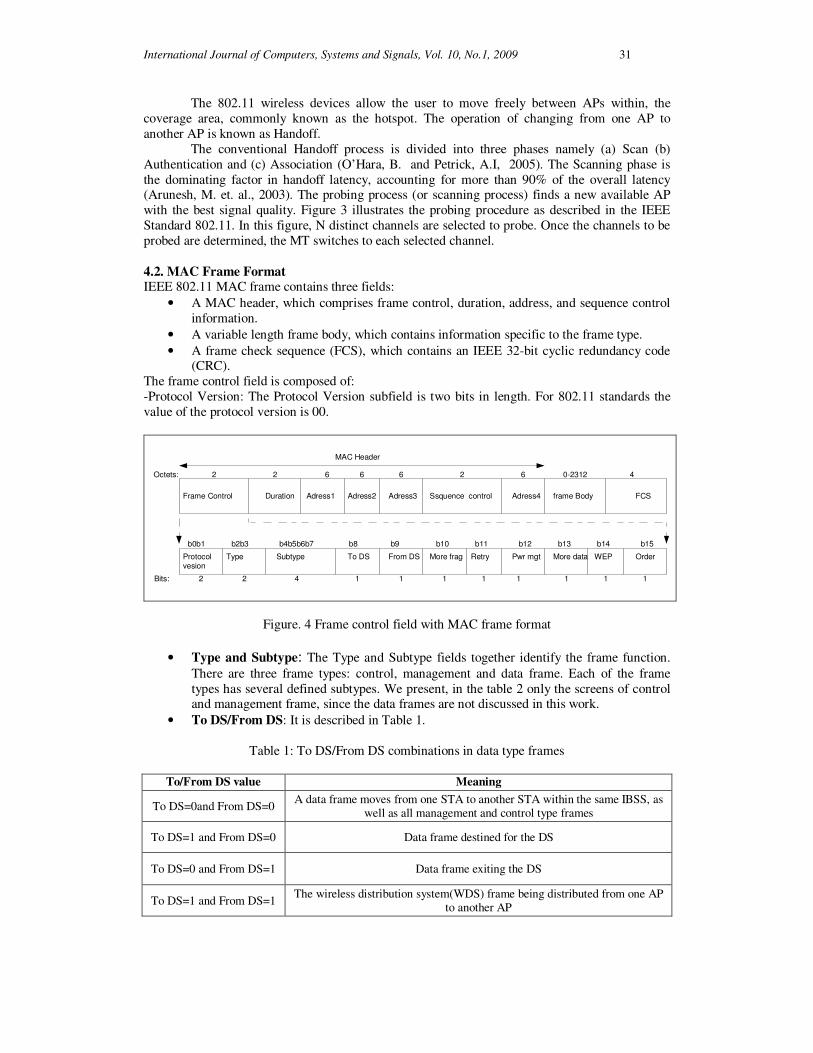
International Journal of Computers, Systems and Signals, Vol. 10, No.1, 2009 31
The 802.11 wireless devices allow the user to move freely between APs within, the
coverage area, commonly known as the hotspot. The operation of changing from one AP to
another AP is known as Handoff.
The conventional Handoff process is divided into three phases namely (a) Scan (b)
Authentication and (c) Association (O’Hara, B. and Petrick, A.I, 2005). The Scanning phase is
the dominating factor in handoff latency, accounting for more than 90% of the overall latency (Arunesh, M. et. al., 2003). The probing process (or scanning process) finds a new available AP
with the best signal quality. Figure 3 illustrates the probing procedure as described in the IEEE
Standard 802.11. In this figure, N distinct channels are selected to probe. Once the channels to be
probed are determined, the MT switches to each selected channel.
4.2. MAC Frame Format IEEE 802.11 MAC frame contains three fields:
• A MAC header, which comprises frame control, duration, address, and sequence control
information.
• A variable length frame body, which contains information specific to the frame type.
• A frame check sequence (FCS), which contains an IEEE 32-bit cyclic redundancy code (CRC).
The frame control field is composed of:
-Protocol Version: The Protocol Version subfield is two bits in length. For 802.11 standards the
value of the protocol version is 00.
Frame Control Duration Adress1 Adress2 Adress3 Ssquence control Adress4 frame Body FCS
Protocol Type Subtype To DS From DS More frag Retry Pwr mgt More data WEP Ordervesion
b0b1 b12b11b10b8b4b5b6b7b2b3 b13 b14 b15b9
2 2 66 6 2 6 0-2312 4
2 2 4 1 1 1 1 1 1 1 1
MAC Header
Octets:
Bits:
Figure. 4 Frame control field with MAC frame format
• Type and Subtype: The Type and Subtype fields together identify the frame function.
There are three frame types: control, management and data frame. Each of the frame
types has several defined subtypes. We present, in the table 2 only the screens of control and management frame, since the data frames are not discussed in this work.
• To DS/From DS: It is described in Table 1.
Table 1: To DS/From DS combinations in data type frames
To/From DS value Meaning
To DS=0and From DS=0 A data frame moves from one STA to another STA within the same IBSS, as
well as all management and control type frames
To DS=1 and From DS=0 Data frame destined for the DS
To DS=0 and From DS=1 Data frame exiting the DS
To DS=1 and From DS=1 The wireless distribution system(WDS) frame being distributed from one AP
to another AP
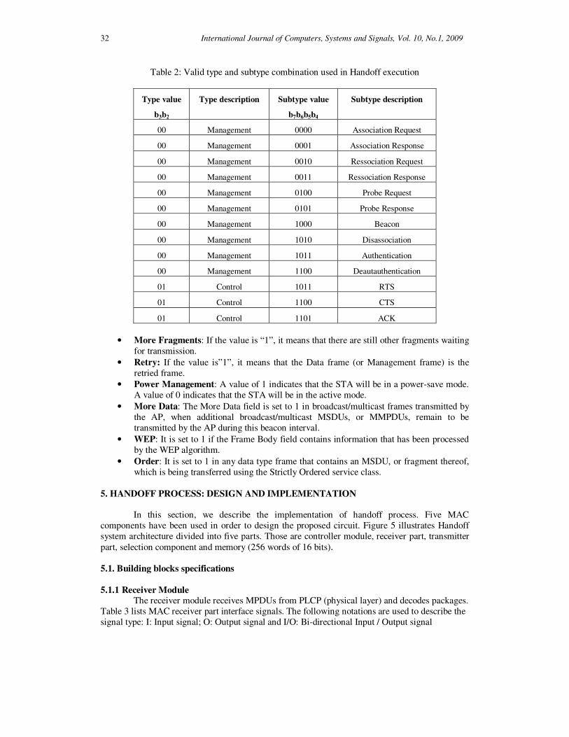
32 International Journal of Computers, Systems and Signals, Vol. 10, No.1, 2009
Table 2: Valid type and subtype combination used in Handoff execution
Type value
b3b2
Type description
Subtype value
b7b6b5b4
Subtype description
00 Management 0000 Association Request
00 Management 0001 Association Response
00 Management 0010 Ressociation Request
00 Management 0011 Ressociation Response
00 Management 0100 Probe Request
00 Management 0101 Probe Response
00 Management 1000 Beacon
00 Management 1010 Disassociation
00 Management 1011 Authentication
00 Management 1100 Deautauthentication
01 Control 1011 RTS
01 Control 1100 CTS
01 Control 1101 ACK
• More Fragments: If the value is “1”, it means that there are still other fragments waiting
for transmission.
• Retry: If the value is”1”, it means that the Data frame (or Management frame) is the
retried frame.
• Power Management: A value of 1 indicates that the STA will be in a power-save mode.
A value of 0 indicates that the STA will be in the active mode.
• More Data: The More Data field is set to 1 in broadcast/multicast frames transmitted by
the AP, when additional broadcast/multicast MSDUs, or MMPDUs, remain to be
transmitted by the AP during this beacon interval.
• WEP: It is set to 1 if the Frame Body field contains information that has been processed
by the WEP algorithm.
• Order: It is set to 1 in any data type frame that contains an MSDU, or fragment thereof,
which is being transferred using the Strictly Ordered service class.
5. HANDOFF PROCESS: DESIGN AND IMPLEMENTATION
In this section, we describe the implementation of handoff process. Five MAC
components have been used in order to design the proposed circuit. Figure 5 illustrates Handoff
system architecture divided into five parts. Those are controller module, receiver part, transmitter
part, selection component and memory (256 words of 16 bits).
5.1. Building blocks specifications
5.1.1 Receiver Module The receiver module receives MPDUs from PLCP (physical layer) and decodes packages.
Table 3 lists MAC receiver part interface signals. The following notations are used to describe the
signal type: I: Input signal; O: Output signal and I/O: Bi-directional Input / Output signal
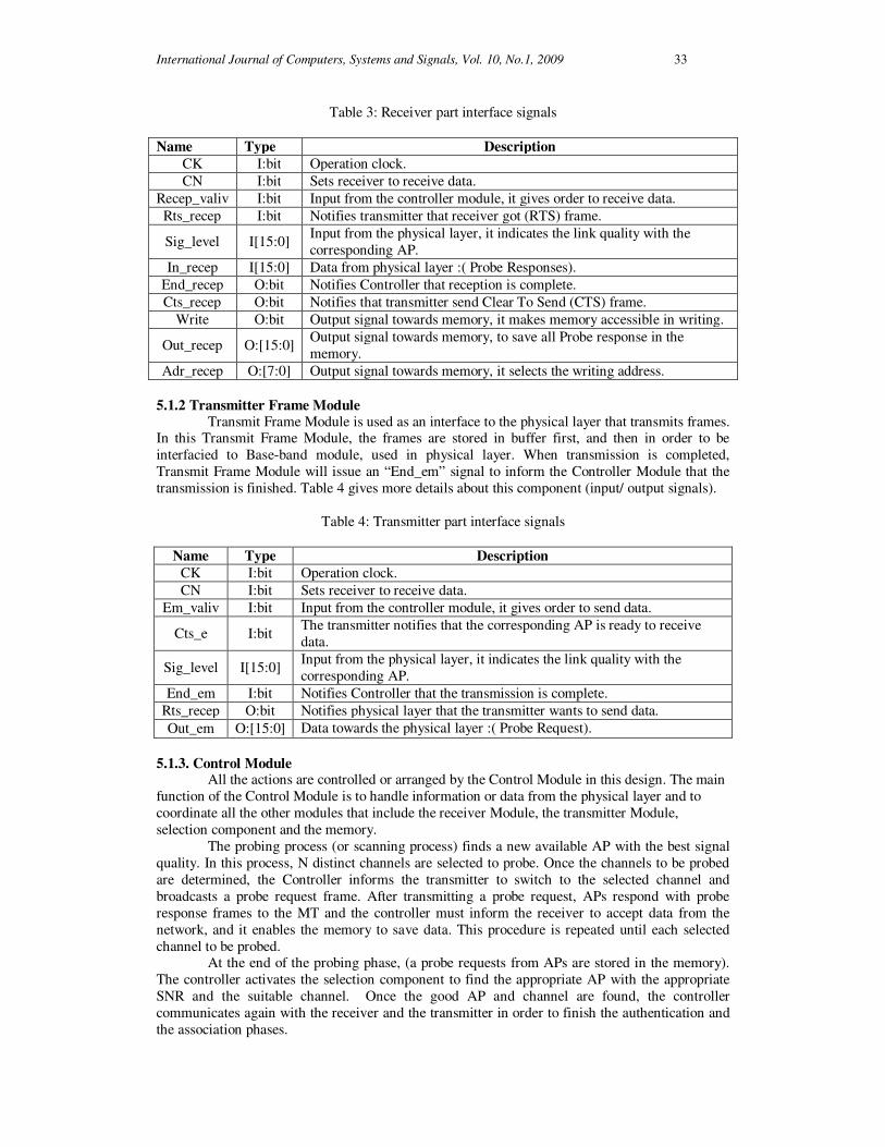
International Journal of Computers, Systems and Signals, Vol. 10, No.1, 2009 33
Table 3: Receiver part interface signals
Name Type Description
CK I:bit Operation clock.
CN I:bit Sets receiver to receive data.
Recep_valiv I:bit Input from the controller module, it gives order to receive data.
Rts_recep I:bit Notifies transmitter that receiver got (RTS) frame.
Sig_level I[15:0] Input from the physical layer, it indicates the link quality with the
corresponding AP.
In_recep I[15:0] Data from physical layer :( Probe Responses).
End_recep O:bit Notifies Controller that reception is complete.
Cts_recep O:bit Notifies that transmitter send Clear To Send (CTS) frame.
Write O:bit Output signal towards memory, it makes memory accessible in writing.
Out_recep O:[15:0] Output signal towards memory, to save all Probe response in the
memory.
Adr_recep O:[7:0] Output signal towards memory, it selects the writing address.
5.1.2 Transmitter Frame Module Transmit Frame Module is used as an interface to the physical layer that transmits frames.
In this Transmit Frame Module, the frames are stored in buffer first, and then in order to be
interfacied to Base-band module, used in physical layer. When transmission is completed,
Transmit Frame Module will issue an “End_em” signal to inform the Controller Module that the
transmission is finished. Table 4 gives more details about this component (input/ output signals).
Table 4: Transmitter part interface signals
Name Type Description
CK I:bit Operation clock.
CN I:bit Sets receiver to receive data.
Em_valiv I:bit Input from the controller module, it gives order to send data.
Cts_e I:bit The transmitter notifies that the corresponding AP is ready to receive
data.
Sig_level I[15:0] Input from the physical layer, it indicates the link quality with the
corresponding AP.
End_em I:bit Notifies Controller that the transmission is complete.
Rts_recep O:bit Notifies physical layer that the transmitter wants to send data.
Out_em O:[15:0] Data towards the physical layer :( Probe Request).
5.1.3. Control Module All the actions are controlled or arranged by the Control Module in this design. The main
function of the Control Module is to handle information or data from the physical layer and to
coordinate all the other modules that include the receiver Module, the transmitter Module,
selection component and the memory.
The probing process (or scanning process) finds a new available AP with the best signal
quality. In this process, N distinct channels are selected to probe. Once the channels to be probed
are determined, the Controller informs the transmitter to switch to the selected channel and
broadcasts a probe request frame. After transmitting a probe request, APs respond with probe
response frames to the MT and the controller must inform the receiver to accept data from the
network, and it enables the memory to save data. This procedure is repeated until each selected
channel to be probed. At the end of the probing phase, (a probe requests from APs are stored in the memory).
The controller activates the selection component to find the appropriate AP with the appropriate
SNR and the suitable channel. Once the good AP and channel are found, the controller
communicates again with the receiver and the transmitter in order to finish the authentication and
the association phases.
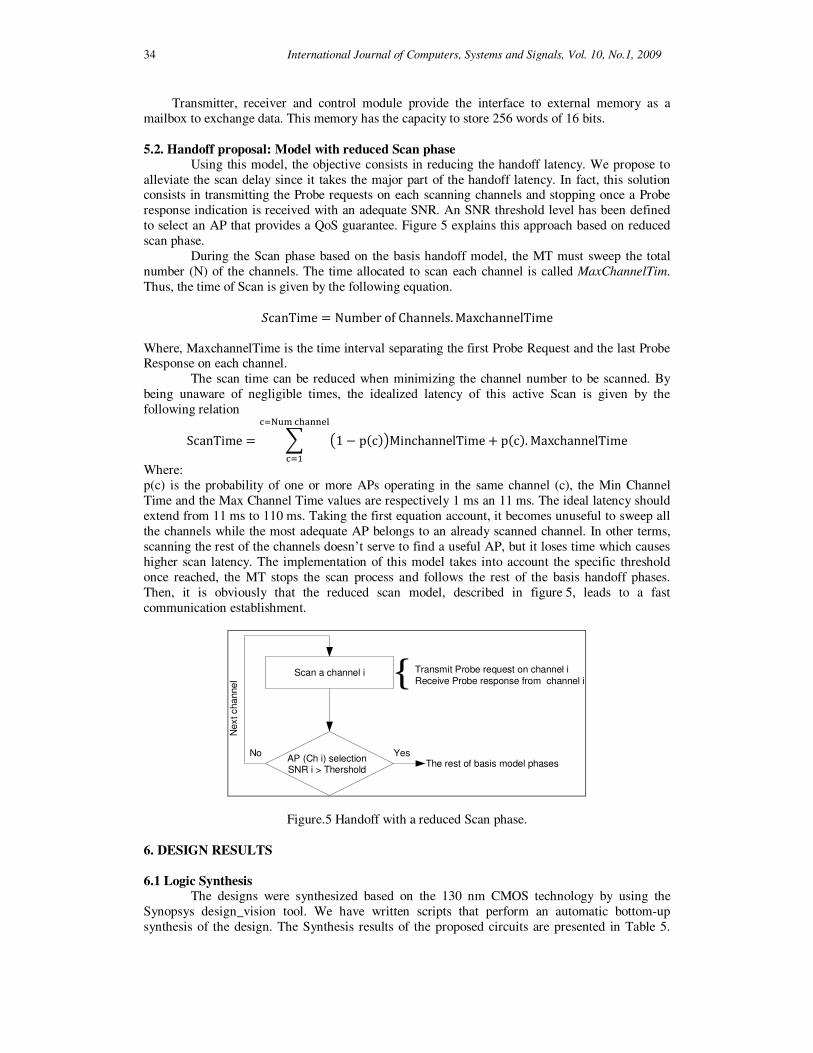
34 International Journal of Computers, Systems and Signals, Vol. 10, No.1, 2009
Transmitter, receiver and control module provide the interface to external memory as a
mailbox to exchange data. This memory has the capacity to store 256 words of 16 bits.
5.2. Handoff proposal: Model with reduced Scan phase Using this model, the objective consists in reducing the handoff latency. We propose to
alleviate the scan delay since it takes the major part of the handoff latency. In fact, this solution consists in transmitting the Probe requests on each scanning channels and stopping once a Probe
response indication is received with an adequate SNR. An SNR threshold level has been defined
to select an AP that provides a QoS guarantee. Figure 5 explains this approach based on reduced
scan phase.
During the Scan phase based on the basis handoff model, the MT must sweep the total
number (N) of the channels. The time allocated to scan each channel is called MaxChannelTim.
Thus, the time of Scan is given by the following equation.
�canTime Number of Channels. MaxchannelTime
Where, MaxchannelTime is the time interval separating the first Probe Request and the last Probe Response on each channel.
The scan time can be reduced when minimizing the channel number to be scanned. By
being unaware of negligible times, the idealized latency of this active Scan is given by the
following relation
ScanTime � �1 � p�c� MinchannelTime ! p�c�. MaxchannelTime"#N%& "'())*+
"#,
Where:
p(c) is the probability of one or more APs operating in the same channel (c), the Min Channel
Time and the Max Channel Time values are respectively 1 ms an 11 ms. The ideal latency should
extend from 11 ms to 110 ms. Taking the first equation account, it becomes unuseful to sweep all
the channels while the most adequate AP belongs to an already scanned channel. In other terms,
scanning the rest of the channels doesn’t serve to find a useful AP, but it loses time which causes
higher scan latency. The implementation of this model takes into account the specific threshold
once reached, the MT stops the scan process and follows the rest of the basis handoff phases.
Then, it is obviously that the reduced scan model, described in figure 5, leads to a fast
communication establishment.
{ Scan a channel i
AP (Ch i) selectionSNR i > Thershold
YesNoThe rest of basis model phases
Transmit Probe request on channel i
Receive Probe response from channel i
Next cha
nne
l
Figure.5 Handoff with a reduced Scan phase.
6. DESIGN RESULTS
6.1 Logic Synthesis The designs were synthesized based on the 130 nm CMOS technology by using the
Synopsys design_vision tool. We have written scripts that perform an automatic bottom-up
synthesis of the design. The Synthesis results of the proposed circuits are presented in Table 5.
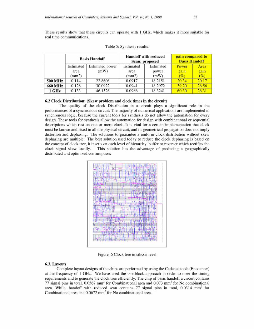
International Journal of Computers, Systems and Signals, Vol. 10, No.1, 2009 35
These results show that these circuits can operate with 1 GHz, which makes it more suitable for
real time communications.
Table 5: Synthesis results.
Basis Handoff
Handoff with reduced
Scan: proposed
gain compared to
Basis Handoff
Estimated
area
(mm2)
Estimated power
(mW)
Estimated
area
(mm2)
Estimated
power
(mW)
Power
gain
(%)
Area
gain
(%)
500 MHz 0.114 22.8606 0.0917 18.2151 20.34 20.17
660 MHz 0.128 30.0922 0.0941 18.2972 39.20 26.56
1 GHz 0.133 46.1526 0.0986 18.3241 60.30 26.31
6.2 Clock Distribution: (Skew problem and clock times in the circuit) The quality of the clock Distribution in a circuit plays a significant role in the
performances of a synchronous circuit. The majority of numerical applications are implemented in synchronous logic, because the current tools for synthesis do not allow the automation for every
design. These tools for synthesis allow the automation for design with combinational or sequential
descriptions which rest on one or more clock. It is vital for a certain implementation that clock
must be known and fixed in all the physical circuit, and its geometrical propagation does not imply
distortion and dephasing. The solutions to guarantee a uniform clock distribution without skew
dephasing are multiple. The best solution used today to reduce the clock dephasing is based on
the concept of clock tree, it inserts on each level of hierarchy, buffer or reverser which rectifies the
clock signal skew locally. This solution has the advantage of producing a geographically
distributed and optimized consumption.
Figure. 6 Clock tree in silicon level
6.3. Layouts Complete layout designs of the chips are performed by using the Cadence tools (Encounter)
at the frequency of 1 GHz. We have used the one-block approach in order to meet the timing
requirements and to generate the clock tree efficiently. The chip of basis handoff a circuit contains
77 signal pins in total, 0.0567 mm2 for Combinational area and 0.073 mm2 for No combinational
area. While, handoff with reduced scan contains 77 signal pins in total, 0.0314 mm2 for
Combinational area and 0.0672 mm2 for No combinational area.
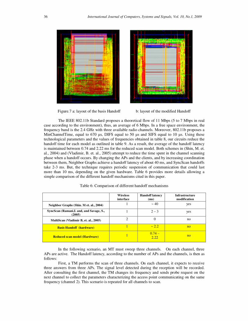
36 International Journal of Computers, Systems and Signals, Vol. 10, No.1, 2009
Figure.7 a: layout of the basis Handoff b: layout of the modified Handoff
The IEEE 802.11b Standard proposes a theoretical flow of 11 Mbps (5 to 7 Mbps in real
case according to the environment), thus, an average of 6 Mbps. In a free space environment, the frequency band is the 2.4 GHz with three available radio channels. Moreover, 802.11b proposes a
MinChannelTime, equal to 670 µs, DIFS equal to 50 µs and SIFS equal to 10 µs. Using these
technological parameters and the values of frequencies obtained in table 8, our circuits reduce the
handoff time for each model as outlined in table 9. As a result, the average of the handoff latency
is maintained between 0.74 and 2.22 ms for the reduced scan model. Both schemes in (Shin, M. et.
al., 2004) and (Vladimir, B. et. al., 2005) attempt to reduce the time spent in the channel scanning
phase when a handoff occurs. By changing the APs and the clients, and by increasing coordination
between them, Neighbor Graphs achieve a handoff latency of about 40 ms, and SyncScan handoffs
take 2-3 ms. But, the technique requires periodic suspension of communication that could last
more than 10 ms, depending on the given hardware. Table 6 provides more details allowing a
simple comparison of the different handoff mechanisms cited in this paper.
Table 6: Comparison of different handoff mechanisms
Wireless
interface
Handoff latency
(ms)
Infrastructure
modification
Neighbor Graphs (Shin. M et. al., 2004) 1 ~ 40 yes
SyncScan (Ramani,I. and, and Savage, S.,
(2005) 1 2 – 3 yes
MultiScan (Vladimir B, et. al., 2005) 2 0 no
Basis Handoff (hardware) 1 ~ 2.2 no
Reduced scan model (Hardware) 1 0.74 – 2.22
no
In the following scenario, an MT must sweep three channels. On each channel, three
APs are active. The Handoff latency, according to the number of APs and the channels, is then as
follows:
First, a TM performs the scan of three channels. On each channel, it expects to receive three answers from three APs. The signal level detected during the reception will be recorded.
After consulting the first channel, the TM changes its frequency and sends probe request on the
next channel to collect the parameters characterizing the access point communicating on the same
frequency (channel 2). This scenario is repeated for all channels to scan.
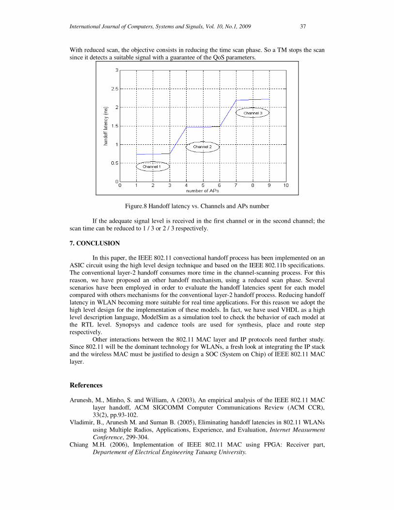
International Journal of Computers, Systems and Signals, Vol. 10, No.1, 2009 37
With reduced scan, the objective consists in reducing the time scan phase. So a TM stops the scan
since it detects a suitable signal with a guarantee of the QoS parameters.
Figure.8 Handoff latency vs. Channels and APs number
If the adequate signal level is received in the first channel or in the second channel; the
scan time can be reduced to 1 / 3 or 2 / 3 respectively.
7. CONCLUSION
In this paper, the IEEE 802.11 convectional handoff process has been implemented on an
ASIC circuit using the high level design technique and based on the IEEE 802.11b specifications.
The conventional layer-2 handoff consumes more time in the channel-scanning process. For this
reason, we have proposed an other handoff mechanism, using a reduced scan phase. Several
scenarios have been employed in order to evaluate the handoff latencies spent for each model
compared with others mechanisms for the conventional layer-2 handoff process. Reducing handoff
latency in WLAN becoming more suitable for real time applications. For this reason we adopt the
high level design for the implementation of these models. In fact, we have used VHDL as a high
level description language, ModelSim as a simulation tool to check the behavior of each model at
the RTL level. Synopsys and cadence tools are used for synthesis, place and route step
respectively.
Other interactions between the 802.11 MAC layer and IP protocols need further study. Since 802.11 will be the dominant technology for WLANs, a fresh look at integrating the IP stack
and the wireless MAC must be justified to design a SOC (System on Chip) of IEEE 802.11 MAC
layer.
References
Arunesh, M., Minho, S. and William, A (2003), An empirical analysis of the IEEE 802.11 MAC
layer handoff, ACM SIGCOMM Computer Communications Review (ACM CCR),
33(2), pp.93-102.
Vladimir, B., Arunesh M. and Suman B. (2005), Eliminating handoff latencies in 802.11 WLANs
using Multiple Radios, Applications, Experience, and Evaluation, Internet Measurment
Conference, 299-304.
Chiang M.H. (2006), Implementation of IEEE 802.11 MAC using FPGA: Receiver part,
Departement of Electrical Engineering Tatuang University.
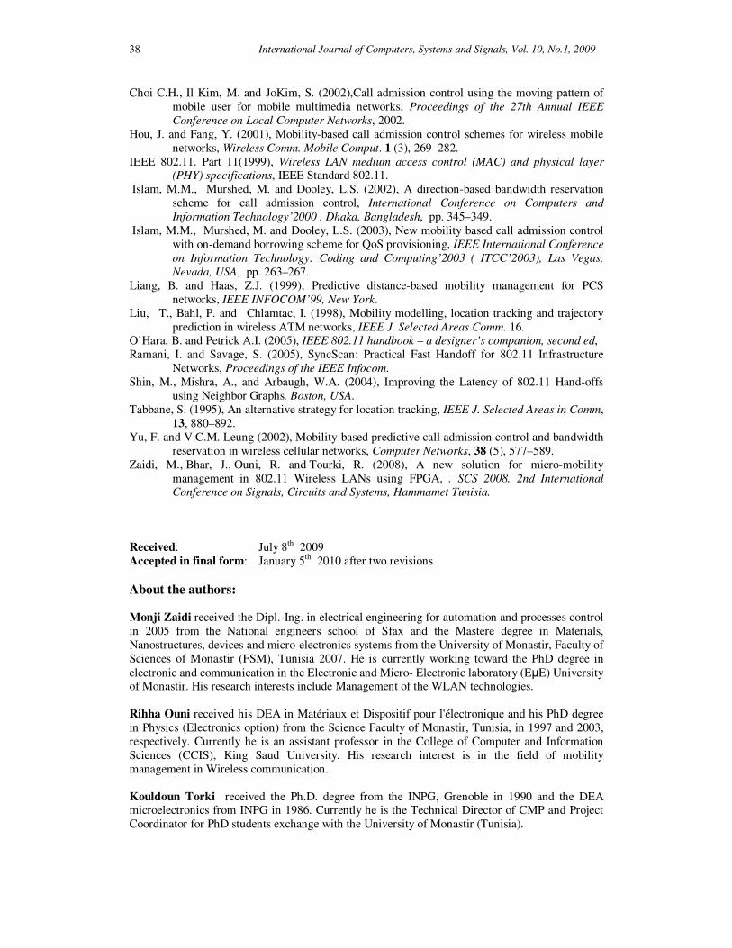
38 International Journal of Computers, Systems and Signals, Vol. 10, No.1, 2009
Choi C.H., Il Kim, M. and JoKim, S. (2002),Call admission control using the moving pattern of
mobile user for mobile multimedia networks, Proceedings of the 27th Annual IEEE
Conference on Local Computer Networks, 2002.
Hou, J. and Fang, Y. (2001), Mobility-based call admission control schemes for wireless mobile
networks, Wireless Comm. Mobile Comput. 1 (3), 269–282.
IEEE 802.11. Part 11(1999), Wireless LAN medium access control (MAC) and physical layer
(PHY) specifications, IEEE Standard 802.11.
Islam, M.M., Murshed, M. and Dooley, L.S. (2002), A direction-based bandwidth reservation
scheme for call admission control, International Conference on Computers and
Information Technology’2000 , Dhaka, Bangladesh, pp. 345–349.
Islam, M.M., Murshed, M. and Dooley, L.S. (2003), New mobility based call admission control
with on-demand borrowing scheme for QoS provisioning, IEEE International Conference
on Information Technology: Coding and Computing’2003 ( ITCC’2003), Las Vegas,
Nevada, USA, pp. 263–267.
Liang, B. and Haas, Z.J. (1999), Predictive distance-based mobility management for PCS
networks, IEEE INFOCOM’99, New York.
Liu, T., Bahl, P. and Chlamtac, I. (1998), Mobility modelling, location tracking and trajectory
prediction in wireless ATM networks, IEEE J. Selected Areas Comm. 16. O’Hara, B. and Petrick A.I. (2005), IEEE 802.11 handbook – a designer’s companion, second ed,
Ramani, I. and Savage, S. (2005), SyncScan: Practical Fast Handoff for 802.11 Infrastructure
Networks, Proceedings of the IEEE Infocom.
Shin, M., Mishra, A., and Arbaugh, W.A. (2004), Improving the Latency of 802.11 Hand-offs
using Neighbor Graphs, Boston, USA.
Tabbane, S. (1995), An alternative strategy for location tracking, IEEE J. Selected Areas in Comm,
13, 880–892.
Yu, F. and V.C.M. Leung (2002), Mobility-based predictive call admission control and bandwidth
reservation in wireless cellular networks, Computer Networks, 38 (5), 577–589.
Zaidi, M., Bhar, J., Ouni, R. and Tourki, R. (2008), A new solution for micro-mobility
management in 802.11 Wireless LANs using FPGA, . SCS 2008. 2nd International
Conference on Signals, Circuits and Systems, Hammamet Tunisia.
Received: July 8th 2009
Accepted in final form: January 5th 2010 after two revisions
About the authors: Monji Zaidi received the Dipl.-Ing. in electrical engineering for automation and processes control
in 2005 from the National engineers school of Sfax and the Mastere degree in Materials,
Nanostructures, devices and micro-electronics systems from the University of Monastir, Faculty of
Sciences of Monastir (FSM), Tunisia 2007. He is currently working toward the PhD degree in
electronic and communication in the Electronic and Micro- Electronic laboratory (EµE) University of Monastir. His research interests include Management of the WLAN technologies.
Rihha Ouni received his DEA in Matériaux et Dispositif pour l'électronique and his PhD degree
in Physics (Electronics option) from the Science Faculty of Monastir, Tunisia, in 1997 and 2003,
respectively. Currently he is an assistant professor in the College of Computer and Information
Sciences (CCIS), King Saud University. His research interest is in the field of mobility
management in Wireless communication.
Kouldoun Torki received the Ph.D. degree from the INPG, Grenoble in 1990 and the DEA microelectronics from INPG in 1986. Currently he is the Technical Director of CMP and Project
Coordinator for PhD students exchange with the University of Monastir (Tunisia).
International Journal of Computers, Systems and Signals, Vol. 10, No.1, 2009 39
Rached Tourki was born in Tunis, on May 13 1948. He received the B.S. degree in Physics
(Electronics option) from Tunis University, in 1970; the M.S. and the Ph.D. in Electronics from
Orsay Electronic Institute, Paris-south University in 1971 and 1973 respectively. From 1973 to
1974 he served as Microelectronics Engineer in Thomson-CSF. He received the Doctorat d’etat in
Physics from Nice University in 1979. Since this date he has been Professor in Microelectronics
and Microprocessors with the Physics department in the Faculty des of Sciences of Monastir. His researches interests are digital signal processing and hardware–software codesign for rapid
prototyping in telecommunications.
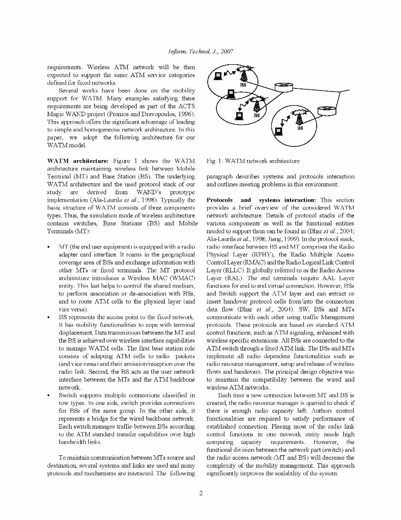
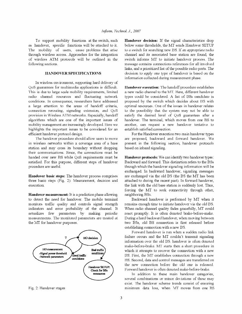
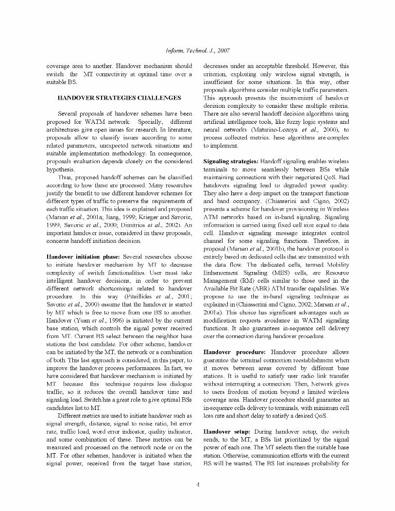
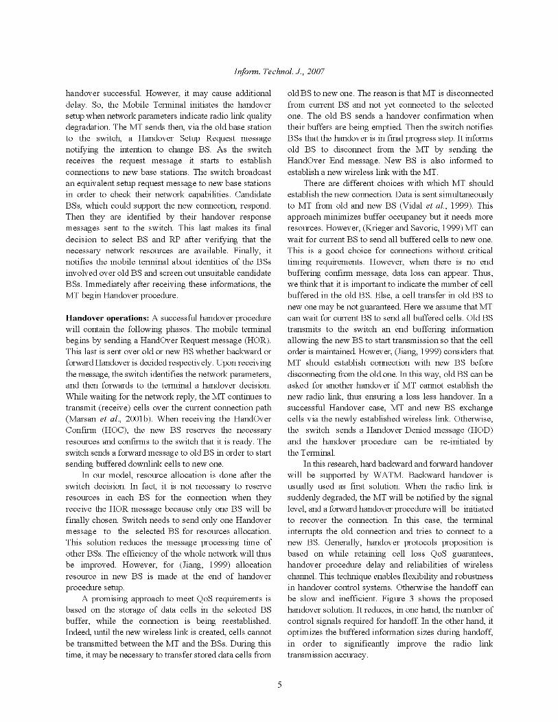
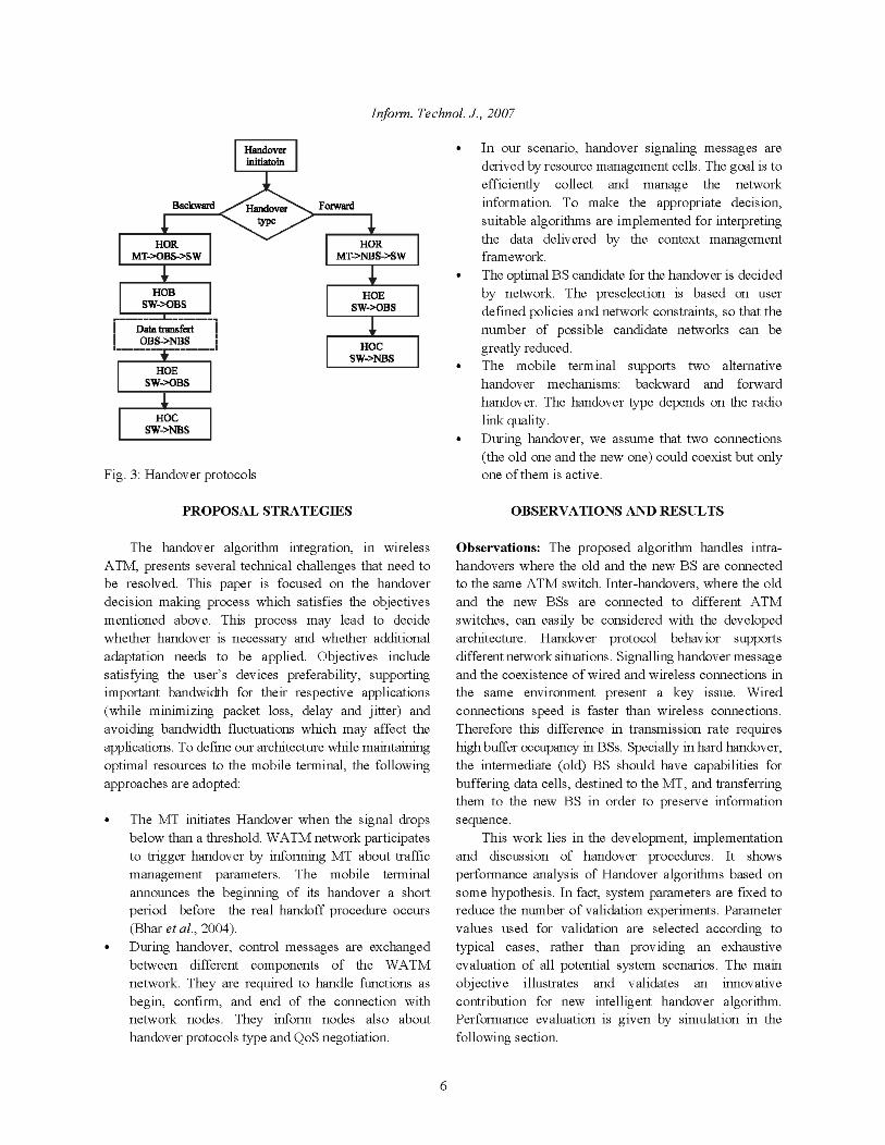
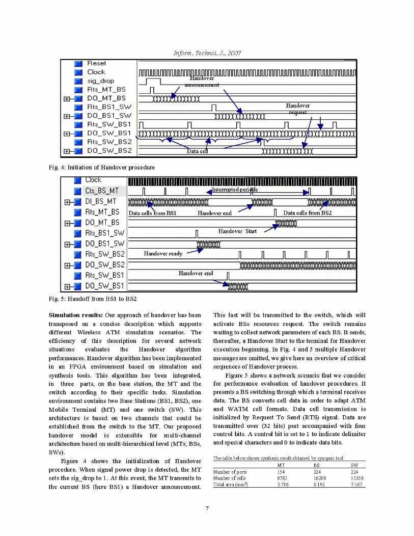
Handover Strategies Challenges in Wireless ATM
Networks Jamila Bhar, Ridha Ouni, Kholdoun Torki, and Salem Nasri
Abstract—To support user mobility for a wireless network new
mechanisms are needed and are fundamental, such as paging, location updating, routing, and handover. Also an important key feature is mobile QoS offered by the WATM. Several ATM network protocols should be updated to implement mobility management and to maintain the already ATM QoS over wireless ATM networks. A survey of the various schemes and types of handover is provided. Handover procedure allows guarantee the terminal connection reestablishment when it moves between areas covered by different base stations. It is useful to satisfy user radio link transfer without interrupting a connection. However, failure to offer efficient solutions will result in handover important packet loss, severe delays and degradation of QoS offered to the applications.
This paper reviews the requirements, characteristics and open issues of wireless ATM, particularly with regard to handover. It introduces key aspects of WATM and mobility extensions, which are added in the fixed ATM network. We propose a flexible approach for handover management that will minimize the QoS deterioration. Functional entities of this flexible approach are discussed in order to achieve minimum impact on the connection quality when a MT crosses the BS.
Keywords—Handover, HDL synthesis, QoS, Wireless ATM.
I. INTRODUCTION HE Asynchronous Transfer Mode (ATM) is a data transport technology that supports a single high speed
infrastructure for integrated broadband communication involving voice, video and data. ATM technology combines some important features: short fixed-size packets or cells, virtual circuits, statistical multiplexing, and integrated services. All these concepts together provide a uniform framework that guarantees traffic with quality of service (QoS) [8].
Wireless ATM (WATM) is mainly considered as an extension of ATM network issue. WATM will be advantageous to support the seamless delivery of multimedia flows with high Quality of Service (QoS). WATM must in all cases allow the network to guarantee a connection continuity of MT.
To support user mobility for a wireless network additional protocols are needed and are fundamental. They mainly refer to handover protocols, routing, and location management. Thus, maintaining QoS guarantees demands to integrate mobility support functions.
This paper introduces the mobility management solutions characteristics of Wireless ATM network. It presents an extended Handover technique for terminal mobility support in
WATM networks. WATM is able to deploy different Handover types, which are intended to manage different network event scenarios. For this purpose, several specific functionalities and algorithms are proposed. In our approach, improved backward and forward hard handover protocols were been developed for switching MT active connections from one base station to another. This approach aimed at defining a solution with optimal method for applying handover in WATM environment. The emphasis was especially on deploying innovative process while maintaining Qos parameters. So, some details of the proposed idea are explained and performed by synthesis and validation phase.
The paper is organized as follows. First, we give an overview of handover protocols. The second section outlines the testing approach adopted for our architecture. Technical challenges are presented and discussed. Then, Handover buffering performances are analyzed and their requirements are explained. Finally, description of our design, synthesis and simulation phases are described and conclusions are given.
II. HANDOVER PROTOCOLS SPECIFICATIONS Handover term refer to different approaches to supporting
mobility aspects. Distinctions between different propositions can be made according to the performance characteristics, diversity steps, state transitions, and control modes of handover techniques. Generally, Handover can be defined as the process by which an active MT changes its point of attachment to the network, or when such a change is attempted. The access network may provide features to minimize the interruption to sessions in progress.
There are different types of handover classified according to different aspects involved in the handover. We can then identify handover types such as backward and forward. This distinction refers to handover steps and to the BSs through which the handover signaling information will be exchanged. In backward handover, signaling messages are exchanged via the old BS (the BS the MT has been attached to during the recent past). Handover scenario, in this case is composed of two stages: setup and handoff. In forward handover, the link with the old base station is suddenly lost. Thus, the MT is forced to seek connectivity through other, neighboring BSs.
In this paper, hard backward and forward handover will be supported by WATM. Backward handover is usually used as first solution. When the radio link is suddenly degraded, the MT will be notified by the signal level, and a forward handover procedure will be initiated to recover the connection.
T
INTERNATIONAL JOURNAL OF APPLIED MATHEMATICS AND COMPUTER SCIENCES VOL. 4 NO. 2 2007 ISSN 1305-5313
ENFORMATIKA VOL. 4 NO. 2 2007 ISSN 1305-5313 636 © 2007 WASET.ORG
In this case, the terminal interrupts the old connection and tries to connect to a new BS. In the following section, we present handover management strategy based on inband signaling.
III. HANDOVER MANAGEMENT STRATEGY
A. Proposal Architecture The handover algorithm integration, in wireless ATM,
presents several technical challenges that need to be resolved. This paper is focused on the handover decision making process which satisfies the objectives mentioned above. This process may lead to decide whether handover is necessary and whether additional adaptation needs to be applied. Objectives include satisfying the user’s devices preferability, supporting important bandwidth for their respective applications and avoiding data loss which may affect the applications.
The integrated architecture defines the following main entities: - Entity at base station: depending on a traffic situation, it can play a role of old or new BS. - Entity at switch node: it is responsible to collect traffic parameters. It manages information from different BSs. - Entity at mobile terminal: it makes final Handover decision. Terminal decides about handover type and which BS is to be selected for the handover. We use the MT because it is more scalable to make decision by itself, especially in degraded situation.
Handover entities are integrated at layer 2 when a handover appears in the same clustered area (BSs attached to the same switch). This type of handover is transparent to the routing functionalities (it requires a simply link layer reconfiguration without any mobility implications) [8].
Entities listed below are described with VHDL language. Implementing handover mechanism with VHDL description poses some specific constraints. The development of several nodes of the network (BSs, MTs) requires traffic management of simultaneous connexions. Other constraint that must be considered is to provide to mobile terminal parameter for handover decision at the right time, with most newly information about traffic conditions. For this purpose, traffic collected parameters are sent periodically to MT.
The steps for handover algorithm are detailed at the following.
B. Phases of Handover Strategy To define our architecture while maintaining optimal
resources to the mobile terminal, the following approaches are adopted: A handover approach adopts a mobile-initiated handover type. The MT makes the initial decision to initiate the handover. However, the WATM network participates to trigger handover by informing MT about traffic management parameters in order to select suitable BS candidates.
In a prediction phase, the mobile terminal monitors traffic quality and controls signal strength indicators and error probability of the channel. It is then periodically informed
with collected information using handover cell. When receiving these parameters, MT actualizes few stored parameters for handover decision algorithm. The MT initiates Handover when the signal drops below than a threshold.
If the switch is informed through old BS about a new handover procedure, it requests BSs about information relevant to the Handover Decision. Collected information will be filtered. The switch sends, to the MT, a BSs list prioritized by the signal power of each one. The Handover Decision process at MT entity is parameterized with this information. In consequence, the MT sends via the old base station to the switch, a Handover Setup Request message notifying the intention to change to the selected BS. Otherwise, communication efforts with the current BS will be wasted. The BS list increases probability for handover successful. However, it may cause additional delay.
From these steps, we can see that this process ensures that the most up-to-date information is used for handover decision.
During handover, control messages are exchanged between different components of the WATM network. They are required to handle functions as begin, confirm, and end of the connection with network nodes. They inform nodes also about handover protocols type and QoS negotiation. Handoff signaling enables wireless terminals to move seamlessly between BSs while maintaining connections with their negotiated QoS. Bad handovers signaling lead to degraded power quality. They also have a deep impact on the transport functions and band occupancy.
In our model, resource allocation is done after the switch decision. In fact, it is not necessary to reserve resources in each BS for the connection when they receive the HOR message because only one BS will be finally chosen. Switch needs to send only one Handover message to the selected BS for resources allocation. This solution reduces the message processing time of other BSs. The efficiency of the whole network will thus be improved.
IV. ANOTHER ISSUES AND CHALLENGES IN WATM
A. Signaling Strategies Handoff signaling enables wireless terminals to move
seamlessly between BSs while maintaining connections with their negotiated QoS. Bad handovers signaling lead to degraded power quality. They also have a deep impact on the transport functions and band occupancy. [1] Presents a scheme for handover provisioning in Wireless ATM networks based on in-band signaling. Signaling information is carried using fixed cell size equal to data cell. Handover signaling message integrates control channel for some signaling functions. Therefore, in proposal [8], the handover protocol is entirely based on dedicated cells that are transmitted with the data flow. The dedicated cells, termed Mobility Enhancement Signaling (MES) cells, are Resource Management (RM) cells similar to those used in the Available Bit Rate (ABR) ATM transfer capabilities. We propose to use the in-band signaling technique as explained in [1]-[8]. The goal is to efficiently collect and manage the network information. This choice has
INTERNATIONAL JOURNAL OF APPLIED MATHEMATICS AND COMPUTER SCIENCES VOL. 4 NO. 2 2007 ISSN 1305-5313
ENFORMATIKA VOL. 4 NO. 2 2007 ISSN 1305-5313 637 © 2007 WASET.ORG
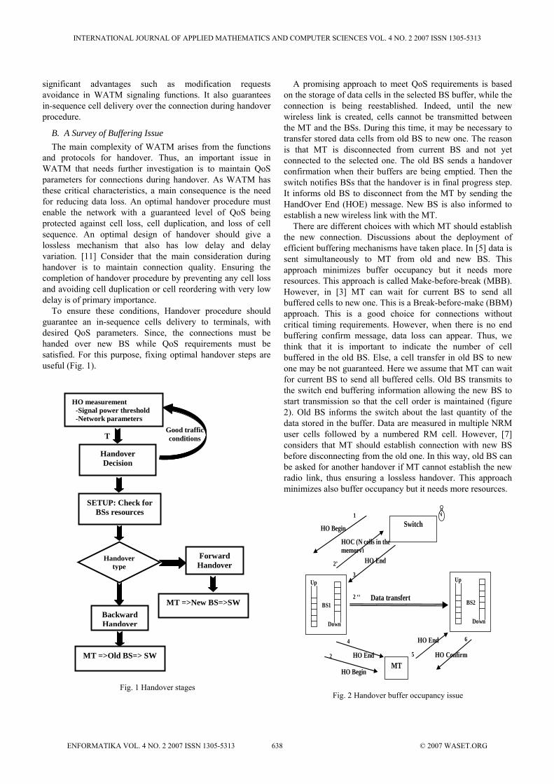
significant advantages such as modification requests avoidance in WATM signaling functions. It also guarantees in-sequence cell delivery over the connection during handover procedure.
B. A Survey of Buffering Issue The main complexity of WATM arises from the functions
and protocols for handover. Thus, an important issue in WATM that needs further investigation is to maintain QoS parameters for connections during handover. As WATM has these critical characteristics, a main consequence is the need for reducing data loss. An optimal handover procedure must enable the network with a guaranteed level of QoS being protected against cell loss, cell duplication, and loss of cell sequence. An optimal design of handover should give a lossless mechanism that also has low delay and delay variation. [11] Consider that the main consideration during handover is to maintain connection quality. Ensuring the completion of handover procedure by preventing any cell loss and avoiding cell duplication or cell reordering with very low delay is of primary importance.
To ensure these conditions, Handover procedure should guarantee an in-sequence cells delivery to terminals, with desired QoS parameters. Since, the connections must be handed over new BS while QoS requirements must be satisfied. For this purpose, fixing optimal handover steps are useful (Fig. 1).
Handover type
HO measurement -Signal power threshold -Network parameters
SETUP: Check for BSs resources
MT =>New BS=>SW
Backward Handover
Forward Handover
MT =>Old BS=> SW
Handover Decision
Good traffic conditions T
Fig. 1 Handover stages
A promising approach to meet QoS requirements is based on the storage of data cells in the selected BS buffer, while the connection is being reestablished. Indeed, until the new wireless link is created, cells cannot be transmitted between the MT and the BSs. During this time, it may be necessary to transfer stored data cells from old BS to new one. The reason is that MT is disconnected from current BS and not yet connected to the selected one. The old BS sends a handover confirmation when their buffers are being emptied. Then the switch notifies BSs that the handover is in final progress step. It informs old BS to disconnect from the MT by sending the HandOver End (HOE) message. New BS is also informed to establish a new wireless link with the MT.
There are different choices with which MT should establish the new connection. Discussions about the deployment of efficient buffering mechanisms have taken place. In [5] data is sent simultaneously to MT from old and new BS. This approach minimizes buffer occupancy but it needs more resources. This approach is called Make-before-break (MBB). However, in [3] MT can wait for current BS to send all buffered cells to new one. This is a Break-before-make (BBM) approach. This is a good choice for connections without critical timing requirements. However, when there is no end buffering confirm message, data loss can appear. Thus, we think that it is important to indicate the number of cell buffered in the old BS. Else, a cell transfer in old BS to new one may be not guaranteed. Here we assume that MT can wait for current BS to send all buffered cells. Old BS transmits to the switch end buffering information allowing the new BS to start transmission so that the cell order is maintained (figure 2). Old BS informs the switch about the last quantity of the data stored in the buffer. Data are measured in multiple NRM user cells followed by a numbered RM cell. However, [7] considers that MT should establish connection with new BS before disconnecting from the old one. In this way, old BS can be asked for another handover if MT cannot establish the new radio link, thus ensuring a lossless handover. This approach minimizes also buffer occupancy but it needs more resources.
HO Begin
5
64
3
2 ‘‘
2’
2
1
Data transfert
MT
Up BS2 Down
Up BS1 Down
HO Begin
HOC (N cells in the memory)
Switch
HO End
HO End
HO End
HO Confirm
Fig. 2 Handover buffer occupancy issue
INTERNATIONAL JOURNAL OF APPLIED MATHEMATICS AND COMPUTER SCIENCES VOL. 4 NO. 2 2007 ISSN 1305-5313
ENFORMATIKA VOL. 4 NO. 2 2007 ISSN 1305-5313 638 © 2007 WASET.ORG
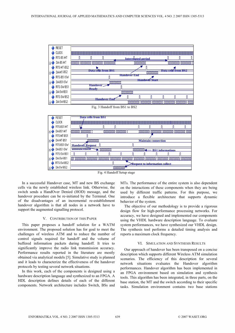
In a successful Handover case, MT and new BS exchange
cells via the newly established wireless link. Otherwise, the switch sends a HandOver Denied (HOD) message, and the handover procedure can be re-initiated by the Terminal. One of the disadvantages of an incremental re-establishment handover algorithm is that all nodes in a network have to support the augmented signalling protocol.
V. CONTRIBUTION OF THIS PAPER This paper proposes a handoff solution for a WATM
environment. The proposed solution has for goal to meet the challenges of wireless ATM and to reduce the number of control signals required for handoff and the volume of buffered information packets during handoff. It tries to significantly improve the radio link transmission accuracy. Performance results reported in the literature are mostly obtained via analytical models [5]. Simulative study is planned and it leads to characterize the effectiveness of the handover protocols by testing several network situations.
In this work, each of the components is designed using a hardware description language and synthesized to an FPGA. A HDL description defines details of each of the different components. Network architecture includes Switch, BSs and
MTs. The performance of the entire system is also dependent on the interactions of these components when they are being used by different traffic patterns. For this purpose, we introduce a flexible architecture that supports dynamic behavior of the system.
The objective of our methodology is to provide a rigorous design flow for high-performance processing networks. For accuracy, we have designed and implemented our components using the VHDL hardware description language. To evaluate system performances, we have synthesized our VHDL design. The synthesis tool performs a detailed timing analysis and reports a maximum clock frequency.
VI. SIMULATION AND SYNTHESIS RESULTS Our approach of handover has been transposed on a concise
description which supports different Wireless ATM simulation scenarios. The efficiency of this description for several network situations evaluates the Handover algorithm performances. Handover algorithm has been implemented in an FPGA environment based on simulation and synthesis tools. This algorithm has been integrated, in three parts, on the base station, the MT and the switch according to their specific tasks. Simulation environment contains two base stations
Fig. 3 Handoff from BS1 to BS2
Handover Ready
Handover End
Handover Start Handover End
Data cells from BS1 Data cells from BS2
Interrupted period
Fig. 4 Handoff Setup stage
BS1 informations
Data cells from BS1
Maintain connection Handover Request announcement
Request to information collect
INTERNATIONAL JOURNAL OF APPLIED MATHEMATICS AND COMPUTER SCIENCES VOL. 4 NO. 2 2007 ISSN 1305-5313
ENFORMATIKA VOL. 4 NO. 2 2007 ISSN 1305-5313 639 © 2007 WASET.ORG
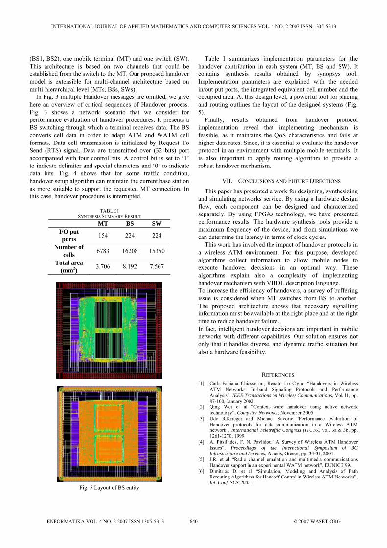
(BS1, BS2), one mobile terminal (MT) and one switch (SW). This architecture is based on two channels that could be established from the switch to the MT. Our proposed handover model is extensible for multi-channel architecture based on multi-hierarchical level (MTs, BSs, SWs).
In Fig. 3 multiple Handover messages are omitted, we give here an overview of critical sequences of Handover process. Fig. 3 shows a network scenario that we consider for performance evaluation of handover procedures. It presents a BS switching through which a terminal receives data. The BS converts cell data in order to adapt ATM and WATM cell formats. Data cell transmission is initialized by Request To Send (RTS) signal. Data are transmitted over (32 bits) port accompanied with four control bits. A control bit is set to ‘1’ to indicate delimiter and special characters and ‘0’ to indicate data bits. Fig. 4 shows that for some traffic condition, handover setup algorithm can maintain the current base station as more suitable to support the requested MT connection. In this case, handover procedure is interrupted.
TABLE I
SYNTHESIS SUMMARY RESULT MT BS SW
I/O put ports 154 224 224
Number of cells 6783 16208 15350
Total area (mm2) 3.706 8.192 7.567
Fig. 5 Layout of BS entity
Table I summarizes implementation parameters for the handover contribution in each system (MT, BS and SW). It contains synthesis results obtained by synopsys tool. Implementation parameters are explained with the needed in/out put ports, the integrated equivalent cell number and the occupied area. At this design level, a powerful tool for placing and routing outlines the layout of the designed systems (Fig. 5).
Finally, results obtained from handover protocol implementation reveal that implementing mechanism is feasible, as it maintains the QoS characteristics and fails at higher data rates. Since, it is essential to evaluate the handover protocol in an environment with multiple mobile terminals. It is also important to apply routing algorithm to provide a robust handover mechanism.
VII. CONCLUSIONS AND FUTURE DIRECTIONS This paper has presented a work for designing, synthesizing
and simulating networks service. By using a hardware design flow, each component can be designed and characterized separately. By using FPGAs technology, we have presented performance results. The hardware synthesis tools provide a maximum frequency of the device, and from simulations we can determine the latency in terms of clock cycles.
This work has involved the impact of handover protocols in a wireless ATM environment. For this purpose, developed algorithms collect information to allow mobile nodes to execute handover decisions in an optimal way. These algorithms explain also a complexity of implementing handover mechanism with VHDL description language. To increase the efficiency of handovers, a survey of buffering issue is considered when MT switches from BS to another. The proposed architecture shows that necessary signalling information must be available at the right place and at the right time to reduce handover failure. In fact, intelligent handover decisions are important in mobile networks with different capabilities. Our solution ensures not only that it handles diverse, and dynamic traffic situation but also a hardware feasibility.
REFERENCES [1] Carla-Fabiana Chiasserini, Renato Lo Cigno “Handovers in Wireless
ATM Networks: In-band Signaling Protocols and Performance Analysis”, IEEE Transactions on Wireless Communications, Vol. l1, pp. 87-100, January 2002.
[2] Qing Wei et al “Context-aware handover using active network technology”; Computer Networks; November 2005.
[3] Udo R.Krieger and Michael Savoric “Performance evaluation of Handover protocols for data communication in a Wireless ATM network”, International Teletraffic Congress (ITC16), vol. 3a & 3b, pp. 1261-1270, 1999.
[4] A. Pitsillides, F. N. Pavlidou “A Survey of Wireless ATM Handover Issues”, Proceedings of the International Symposium of 3G Infrastructure and Services, Athens, Greece, pp. 34-39, 2001.
[5] J.R. et al “Radio channel emulation and multimedia communications Handover support in an experimental WATM network ”, EUNICE’99.
[6] Dimitrios D. et al “Simulation, Modeling and Analysis of Path Rerouting Algorithms for Handoff Control in Wireless ATM Networks”, Int. Conf. SCS’2002.
INTERNATIONAL JOURNAL OF APPLIED MATHEMATICS AND COMPUTER SCIENCES VOL. 4 NO. 2 2007 ISSN 1305-5313
ENFORMATIKA VOL. 4 NO. 2 2007 ISSN 1305-5313 640 © 2007 WASET.ORG
[7] Fan Jiang “Microcellular Handover in Wireless ATM”, Proceedings of the 32nd Hawaii International Conference on System Sciences, 1999.
[8] Marco Ajmone Marsan, et al “Local and Global Handovers Based on In-Band Signaling in Wireless ATM Networks”, Wireless Networks, Vol. 7, No.4, pp. 425-436, ISSN: 1022-0038, July 2001.
[9] Marco Ajmone Marsan, et al “Performance Models of Handover Protocols and Buffering Policies in Mobile Wireless ATM Networks”, IEEE Transactions on Vehicular Technology, Vol. 50, No.4, pp. 925-941, July 2001.
[10] Qing Wei, Kàroly Farkas, Christian Prehofer, Paulo Mendes, Bernhard Plattner “Context-aware handover using active network technology”; Computer Networks; 2006.
[11] Raymond R. Hoarea, Zhu Dinga, Shenchih Tunga, Rami Melhemb, Alex K. Jonesa “A framework for the design, synthesis and cycle-accurate simulation of multiprocessor networks”; J. Parallel Distrib. Comput. 65; 2005.
[12] Nasıf Ekiz, Tara Salih, Sibel Küçüköner and Kemal Fidanboylu “An Overview of Handoff Techniques in Cellular Networks”, International Journal of Information Technology, vol. 2, No. 3, ISSN 1305-239X, 2005.
Jamila Bhar received her Engineering diploma in Electric and her DEA in Communication system from the National School of Engineering of Tunis (ENIT), Tunisia in 2001 and 2002, respectively. Currently, she is a PhD student. Her research interests include protocol adaptation in heterogeneous networks, traffic management and Quality of Service for high speed networks. Her recent work has been in traffic control in WATM network. Ridha Ouni received his doctoral degree in physic (2002) from the Science Faculty of Monastir, Tunisia He is currently an assistant Professor at the Preparatory Institute of Engineering Study of Monastir (IPEIM), Tunisia. His research interests include computer networks, flow and congestion control, interoperability and performance evaluation. He is interested in many areas of hardware/software protocol verification and design for distributed systems. Salem Nasri received his Doctoral degree in automatic control and computer engineering from the National Institute of Applied Sciences of Toulouse France, in June 1985. His research interests are in the fields of computer networks, communication systems and multimedia applications. In May 2001 he obtained the diploma of “Habilitation universitaire”. Since then he has been a professor. He developed collaboration with many laboratories in France such as LSR (Grenoble), CRAN (Nancy), and some other laboratories in Tunisia. Currently he is a professor in the Computer Science Department, Qassim University in the Kingdom of Saudi Arabia.
INTERNATIONAL JOURNAL OF APPLIED MATHEMATICS AND COMPUTER SCIENCES VOL. 4 NO. 2 2007 ISSN 1305-5313
ENFORMATIKA VOL. 4 NO. 2 2007 ISSN 1305-5313 641 © 2007 WASET.ORG
Papiers publiés dans des
CONFERENCES INTERNATIONALES
1. Thamer Alanazi, Ridha Ouni, Traffic Differentiation and Scheduling for QoS support in Vehicular
Sensor Networks, IEEE International Conference on Technological Advances in Electrical, Electronics
and Computer Engineering (TAEECE), Turkey, 2013 (ISBN: 978-1-4673-5611-4).
2. Jihed Khaskhoussi, Ridha Ouni, Enhanced-MPR-CDS approach for self-organization and routing in
WSNs, 1st Taibah University International Conference on Computing and Information Technology Al-
Madinah Al-Munawwarah, Saudi Arabia, 19-21 Rabi II 1433 Hijri (12-14 March 2012)
3. Monji Zaidi, Ridha Ouni, Jamila Bhar and Rached Tourki, A novel positioning technique with low
complexity in wireless LAN: hardware implementation, Proceedings of the World Congress on
Engineering, Vol II, July 6 - 8, 2011, London, U.K (ISSN: 2078-0966).
4. Monji ZAIDI, Jamila BHAR, Ridha OUNI and Rached TOURKI. Reducing Wi-Fi handover delay using a
new positioning process, International Conference on Communications, Computing and Control
Applications (CCCA), Hammamet, pp. 1-6, 2011 (ISBN.978-1-4244-9795-9).
5. M. Z. Hourani, R. Ouni, N. Hussain, Novel Data Harvesting Scheme for Efficient Data Aggregation,
ICW2941, WORLDCOMP'11, USA. 2011. (http://world-comp.org/p2011/ICW2941.pdf)
6. Monji ZAIDI, Rached TOURKI, Ridha OUNI, New geometric Approach to Mobile Position in wireless
LAN reducing complex computations, International Conference on Design & Technology of Integrated
Systems in Nanoscale Era, pp. 1-7, 2010.
7. Jamila BHAR, Ridha OUNI, Salem NASRI, Performance evaluation of compensation-reward
mechanism for resource allocation in wireless networks, The 15th IEEE International Conference on
Electronics, Circuits, and Systems, Malta 31st August to 3rd September 2008, pp 1195-1200.
8. Jamila BHAR, Mongi ZAIDI, Ridha OUNI, Salem NASRI, Performance Evaluation of Fuzzy
Controller for Traffic Stabilization, International Conference on Signals, Circuits & Systems (SCS’08)
November 7-9, 2008, Hammamet (Tunisie).
9. Mongi ZAIDI, Jamila BHAR, Ridha OUNI, Rached TOURKI, A new solutions for micro-mobility
management in 802.11 Wireless LANs using FPGA, International Conference on Signals, Circuits &
Systems (SCS’08) November 7-9, 2008 Hammamet (Tunisie).
10. Jamila BHAR, Ridha OUNI and Salem NASRI, Interopérabilité Ethernet/WATM, International
Conference: Sciences of Electronic, Technologies of Information and Telecommunications, Tunisia,
March 15-20, 2004.
11. Jamila BHAR, Ridha OUNI, Abdelhamid HELALI, Salem NASRI, Improvements of the ABR loop
performances in a wireless ATM network, International Conference on Microelectronic, IEEE
Conference, Gammarth, Tunisia, December 2004.
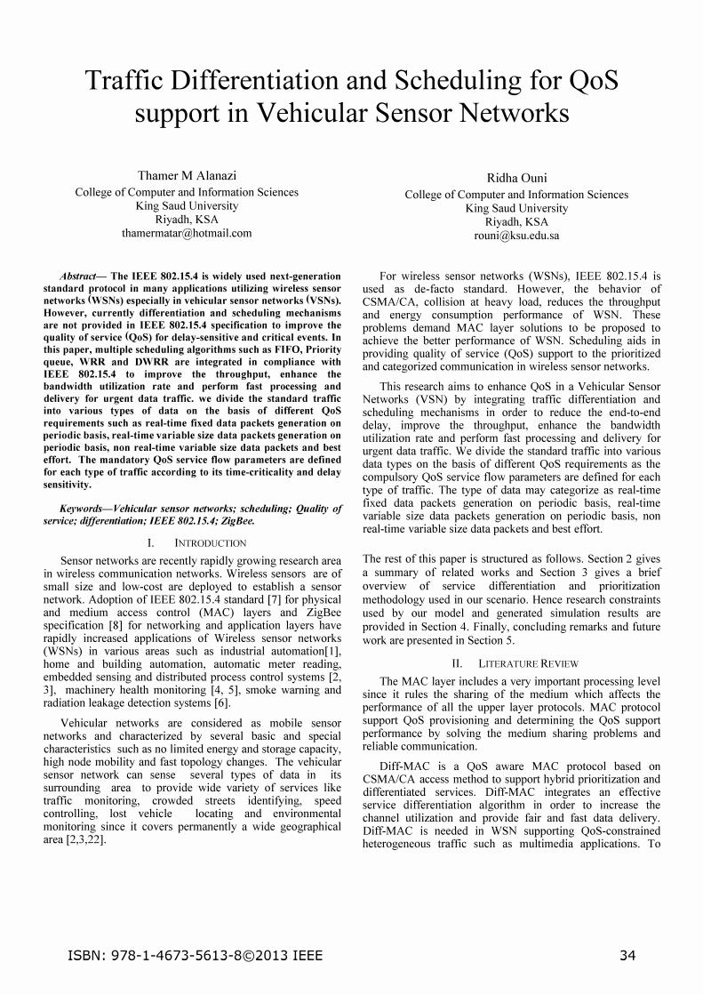
Traffic Differentiation and Scheduling for QoS support in Vehicular Sensor Networks
Thamer M Alanazi College of Computer and Information Sciences
King Saud University Riyadh, KSA
Abstract- The IEEE 802.15.4 is widely used next-generation
standard protocol in many applications utilizing wireless sensor
networks (WSNs) especially in vehicular sensor networks (VSNs).
However, currently differentiation and scheduling mechanisms
are not provided in IEEE 802.15.4 specification to improve the
quality of service (QoS) for delay-sensitive and critical events. In
this paper, multiple scheduling algorithms such as FIFO, Priority
queue, WRR and DWRR are integrated in compliance with
IEEE 802.15.4 to improve the throughput, enhance the
bandwidth utilization rate and perform fast processing and
delivery for urgent data traffic. we divide the standard traffic
into various types of data on the basis of different QoS
requirements such as real-time fixed data packets generation on
periodic basis, real-time variable size data packets generation on
periodic basis, non real-time variable size data packets and best
effort. The mandatory QoS service flow parameters are defined
for each type of traffic according to its time-criticality and delay
sensitivity.
Keywords-Vehicular sensor networks; scheduling; Quality of service; differentiation; IEEE 802.15.4; ZigBee.
I. INTRODUCTION
Sensor networks are recently rapidly growing research area in wireless communication networks. Wireless sensors are of small size and low-cost are deployed to establish a sensor network. Adoption of IEEE 802.15.4 standard [7] for physical and medium access control (MAC) layers and ZigBee specification [8] for networking and application layers have rapidly increased applications of Wireless sensor networks (WSN s) in various areas such as industrial automation[ 1], home and building automation, automatic meter reading, embedded sensing and distributed process control systems [2, 3], machinery health monitoring [4, 5], smoke warning and radiation leakage detection systems [6].
Vehicular networks are considered as mobile sensor networks and characterized by several basic and special characteristics such as no limited energy and storage capacity, high node mobility and fast topology changes. The vehicular sensor network can sense several types of data in its surrounding area to provide wide variety of services like traffic monitoring, crowded streets identifying, speed controlling, lost vehicle locating and environmental monitoring since it covers permanently a wide geographical area [2,3,22].
ISBN: 978-1-4673-5613-8©2013 IEEE
Ridha Ouni College of Computer and Information Sciences
King Saud University Riyadh, KSA
For wireless sensor networks (WSNs), IEEE 802.15.4 is used as de-facto standard. However, the behavior of CSMA/CA, collision at heavy load, reduces the throughput and energy consumption performance of WSN. These problems demand MAC layer solutions to be proposed to achieve the better performance of WSN. Scheduling aids in providing quality of service (QoS) support to the prioritized and categorized communication in wireless sensor networks.
This research aims to enhance QoS in a Vehicular Sensor Networks (VSN) by integrating traffic differentiation and scheduling mechanisms in order to reduce the end-to-end delay, improve the throughput, enhance the bandwidth utilization rate and perform fast processing and delivery for urgent data traffic. We divide the standard traffic into various data types on the basis of different QoS requirements as the compulsory QoS service flow parameters are defined for each type of traffic. The type of data may categorize as real-time fixed data packets generation on periodic basis, real-time variable size data packets generation on periodic basis, non real-time variable size data packets and best effort.
The rest of this paper is structured as follows. Section 2 gives a summary of related works and Section 3 gives a brief overview of service differentiation and prioritization methodology used in our scenario. Hence research constraints used by our model and generated simulation results are provided in Section 4. Finally, concluding remarks and future work are presented in Section 5.
II. LITERATURE REVIEW
The MAC layer includes a very important processing level since it rules the sharing of the medium which affects the performance of all the upper layer protocols. MAC protocol support QoS provisioning and determining the QoS support performance by solving the medium sharing problems and reliable communication.
Diff-MAC is a QoS aware MAC protocol based on CSMA/CA access method to support hybrid prioritization and differentiated services. Diff-MAC integrates an effective service differentiation algorithm in order to increase the channel utilization and provide fair and fast data delivery. Diff-MAC is needed in WSN supporting QoS-constrained heterogeneous traffic such as multimedia applications. To
34
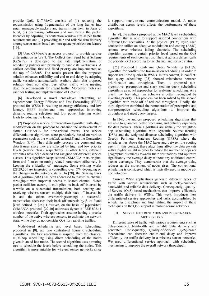
provide QoS, Diff-MAC consists of (1) reducing the retransmission using fragmentation of the long frames into small manageable packets and transmitting them in form of burst, (2) decreasing collisions and minimizing the packet latencies by adjusting its contention window size as per traffic requirements and (3) providing fair and reliable data delivery among sensor nodes based on intra-queue prioritization feature [19].
[5] Uses CSMA/CA as access protocol to provide service differentiation in WSN. The Collect then Send burst Scheme (CoSenS) is developed to facilitate implementation of scheduling policies and primarily to handle its weaknesses. A earliest deadline first and fixed priority are implemented on the top of CoSenS. The results present that the proposed solution enhances reliability and end-to-end delay by adapting traffic variations automatically. Authors claim that proposed solution does not affect best effort traffic while meeting deadline requirements for urgent traffic. Moreover, motes are used for testing and implementation of CoSenS.
[6] Developed a novel cross-layer integrating an asynchronous Energy Efficient and Fast Forwarding (EEFF) protocol for WSNs is resulting to energy efficiency and low latency. EEFF implements new approaches improving dynamic routing selection and low power listening which leads to reducing the latency.
[7] Proposed a service differentiation algorithm with slight modification on the protocol to enhance the achievement of slotted CSMA/CA for time-critical events. The service differentiation algorithms were particularly based on various parameters such as the macHinE, aMaxBE and the Contention Window (CW). They differently process the command and data frames since they are affected by high and low priority levels (service class), respectively. In other terms, different attributes have been defined and assigned for different service classes. This algorithm keeps slotted CSMAICA in its original form and focuses on tuning related parameters effectively in keeping the criticality of messages. Some existing works [28,29,30] are interested in controlling over CW depending on the changes in the network status. In [28], the Sensing Back off Algorithm (SBA) has been addressed to maximize channel throughput with impartial access to shared channel. When packet collision occurs, it multiplies its back off interval by a while on a successful transmission, both sending and receiving wireless sensors multiply their back off interval by 8, and the others overhearing(sensing) a successful transmission decreases their back off intervals by �. a, 8 and � are defined in [28]. However, on the basis of p-persistent CSMA/CA protocol, [29,30] addresses dynamic IEEE 802.11 wireless networks. Their approaches assume having a precise number of the active wireless sensors, to estimate the network state, while they do not consider QoS for real-time traffics.
Node-based scheduling and level based scheduling, proposed in [8], are two centralized heuristic scheduling algorithms. The first algorithm is inspired from the classical multi-hop scheduling using direct scheduling of the nodes given in an ad hoc mode. The second algorithm uses a routing tree to schedule the levels before scheduling the nodes. This algorithm is more suitable for wireless sensor networks since
ISBN: 978-1-4673-5613-8©2013 IEEE
it supports many-to-one communication model. A nodes distribution across levels affects the performance of these algorithms.
In [9], the authors proposed at the MAC level a scheduling algorithm that is able to support assorted connections with different QoS necessities. At the physical (PRY) layer, each connection utilize an adaptive modulation and coding (AMC) scheme over wireless fading channels. The scheduling algorithm assigns a certain priority level based on the QoS requirements of each connection. Then, it adjusts dynamically the priority level according to the channel and service status.
[25] Proposed a Real-Time Query Scheduling (RTQS) algorithm for conflict-free transmission scheduling in order to support real-time queries in WSNs. In this context, in conflictfree query scheduling [25] showed relatedness between prioritization and throughput. Then, it proposed nonpreemptive, preemptive and slack stealing query scheduling algorithms as novel approaches for real-time scheduling. As a result, the first algorithm achieves a better throughput by inverting priority. This problem has been solved by the second algorithm with trade-off of reduced throughput. Finally, the third algorithm combined the remuneration of preemptive and non-preemptive scheduling algorithms to improve the throughput and meet query targets.
In [26], the authors proposed scheduling algorithms that are able to guarantee better processing and delivery especially for data packets. These algorithms are namely the weightedhop scheduling algorithm with Dynamic Source Routing (DSR) and the weighted distance scheduling algorithm with Greedy Perimeter Stateless Routing (GPSR) where the scheduler lies above the MAC layer and between the routing agent. In this context, these algorithms affect the data packets with a higher weight in order to reduce the number of hops (or geographic distances) towards their destinations and optimize significantly the average delay without any additional control packet exchange. They demonstrate that the average delay reduces as the movement of nodes rises. The conventional scheduling is considered which is typically used in mobile adhoc networks.
Current WSN applications generate different types of traffic with various requirements such as delay-bounded, bandwidth and reliable data delivery. Consequently, Qualityof-Service (QoS)-based mechanisms can improve efficiently the traffic delivery in WSNs. This work introduces new differentiated service approaches and tasks accomplished by scheduling disciplines and highlighting the impact of these techniques on the QoS support in mobile sensor networks.
III. SERVICE DIFFERENTIATION AND PRIORITIZATION
METHODOLOGY
Different types of traffic with various requirements such as delay-bounded, bandwidth and reliable data delivery are generated. Consequently, Quality-of-Service (QoS)-based mechanisms can decrease end-to-end delay and improve efficiently the traffic delivery in a wireless sensor networks. We used differentiated service approach with scheduling mechanism to improve the overall network throughput.
35
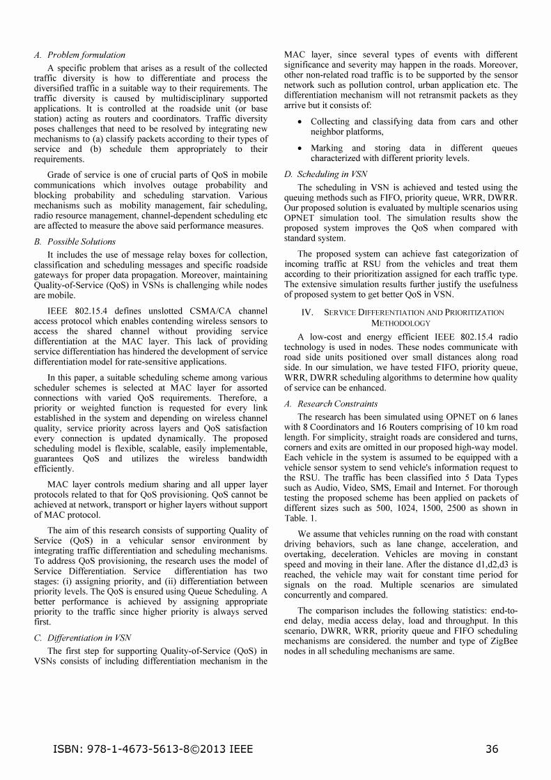
A. Problem formulation
A specific problem that arises as a result of the collected traffic diversity is how to differentiate and process the diversified traffic in a suitable way to their requirements. The traffic diversity is caused by multidisciplinary supported applications. It is controlled at the roadside unit (or base station) acting as routers and coordinators. Traffic diversity poses challenges that need to be resolved by integrating new mechanisms to (a) classify packets according to their types of service and (b) schedule them appropriately to their requirements.
Grade of service is one of crucial parts of QoS in mobile communications which involves outage probability and blocking probability and scheduling starvation. Various mechanisms such as mobility management, fair scheduling, radio resource management, channel-dependent scheduling etc are affected to measure the above said performance measures.
B. Possible Solutions
[t includes the use of message relay boxes for collection, classification and scheduling messages and specific roadside gateways for proper data propagation. Moreover, maintaining Quality-of-Service (QoS) in VSNs is challenging while nodes are mobile.
IEEE 802.15.4 defmes unslotted CSMAICA channel access protocol which enables contending wireless sensors to access the shared channel without providing service differentiation at the MAC layer. This lack of providing service differentiation has hindered the development of service differentiation model for rate-sensitive applications.
[n this paper, a suitable scheduling scheme among various scheduler schemes is selected at MAC layer for assorted connections with varied QoS requirements. Therefore, a priority or weighted function is requested for every lim<established in the system and depending on wireless channel quality, service priority across layers and QoS satisfaction every connection is updated dynamically. The proposed scheduling model is flexible, scalable, easily implementable, guarantees QoS and utilizes the wireless bandwidth efficiently.
MAC layer controls medium sharing and all upper layer protocols related to that for QoS provisioning. QoS cannot be achieved at network, transport or higher layers without support of MAC protocol.
The aim of this research consists of supporting Quality of Service (QoS) in a vehicular sensor environment by integrating traffic differentiation and scheduling mechanisms. To address QoS provisioning, the research uses the model of Service Differentiation. Service differentiation has two stages: (i) assigning priority, and (ii) differentiation between priority levels. The QoS is ensured using Queue Scheduling. A better performance is achieved by assigning appropriate priority to the traffic since higher priority is always served first.
C. Differentiation in VSN
The first step for supporting Quality-of-Service (QoS) in VSNs consists of including differentiation mechanism in the
ISBN: 978-1-4673-5613-8©2013 IEEE
MAC layer, since several types of events with different significance and severity may happen in the roads. Moreover, other non-related road traffic is to be supported by the sensor network such as pollution control, urban application etc. The differentiation mechanism will not retransmit packets as they arrive but it consists of:
• Collecting and classifying data from cars and other neighbor platforms,
• Marking and storing data in different queues characterized with different priority levels.
D. Scheduling in VSN
The scheduling in VSN is achieved and tested using the queuing methods such as F[FO, priority queue, WRR, DWRR. Our proposed solution is evaluated by multiple scenarios using OPNET simulation tool. The simulation results show the proposed system improves the QoS when compared with standard system.
The proposed system can achieve fast categorization of incoming traffic at RSU from the vehicles and treat them according to their prioritization assigned for each traffic type. The extensive simulation results further justify the usefulness of proposed system to get better QoS in VSN.
IV. SERVICE DIFFERENTIATION AND PRIORITIZATION
METHODOLOGY
A low-cost and energy efficient IEEE 802. [5.4 radio technology is used in nodes. These nodes communicate with road side units positioned over small distances along road side. In our simulation, we have tested FIFO, priority queue, WRR, DWRR scheduling algorithms to determine how quality of service can be enhanced.
A. Research Constraints
The research has been simulated using OPNET on 6 lanes with 8 Coordinators and 16 Routers comprising of [0 km road length. For simplicity, straight roads are considered and turns, comers and exits are omitted in our proposed high-way model. Each vehicle in the system is assumed to be equipped with a vehicle sensor system to send vehicle's information request to the RSU. The traffic has been classified into 5 Data Types such as Audio, Video, SMS, Email and Internet. For thorough testing the proposed scheme has been applied on packets of different sizes such as 500, 1024, [500, 2500 as shown in Table. 1.
We assume that vehicles running on the road with constant driving behaviors, such as lane change, acceleration, and overtaking, deceleration. Vehicles are moving in constant speed and moving in their lane. After the distance d 1 ,d2,d3 is reached, the vehicle may wait for constant time period for signals on the road. Multiple scenarios are simulated concurrently and compared.
The comparison includes the following statistics: end-toend delay, media access delay, load and throughput. In this scenario, DWRR, WRR, priority queue and F[FO scheduling mechanisms are considered. the number and type of ZigBee nodes in all scheduling mechanisms are same.
36
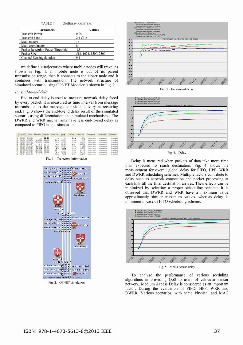
TABLE I. ZIG BEE PARAMETERS
Parameters Values Transmit Power 0.05 Transmit band 2.4 GHz Max. routers 16 Max. coordinators 8 Packet Reception-Power Threshold -85 Packet Size 512,1024,1500,2500 Channel Sensing duration 0.1
we define six trajectories where mobile nodes will travel as shown in Fig. 1. if mobile node is out of its parent transmission range, then it connects to the closer node and it continues with transmission. The network structure of simulated scenario using OPNET Modeler is shown in Fig. 2.
B. End-la-end delay
End-to-end delay is used to measure network delay faced by every packet. it is measured as time interval from message transmission to the message complete delivery at receiving end. Fig. 3 shows the end-to-end delay result of the simulated scenario using differentiation and simulated mechanisms. The DWRR and WRR mechanisms have less end-to-end delay as compared to FIFO in this simulation.
x Pos[m] Y Pos (m] Disl.m:e[m] AUude[m) Tr�yefSe Time 5,,,,",, W�hne AccoxnTime Pf:ch(deQleesj Y�I'I [de�eesl R04[degees] S",od
1 0= 0= "', ,,;, ,,;, 00.00. Aul:oc�e<J ALtClCOOlPlied Urnpeclied
2 0= 81027294 81.027293 0[((0)) 29.17, 0.213674 10_00. 39,17>: AutocOffJlllNJ ALtOCUflP'.J� Umpedied
3 {I268302 206.056165 125,02'3133 0[((0)) 45.01, 6.213782 10.00. lm34.16. AutocOl'l'f'l'l:e<J ALtocornp<J.ed Un,pedied
4 0.5366(5 3)J.011827 6.21428S 2m28.00s Autoeornp<J.ed Auloeomp<.led Umpeclied
5 0 26S3J2 457.45541S 6.2136&4 moos Autocomp<.led ALtocomp<.i.ed Unspeclied
6 Ooo:roJ 581S476ffi mOO,; 4m19.SO, Aulocomp<.led ALtClCOOlPlied Um�lied
.<J5366057Cl6,439'353 124.493530 0[((0)) 10.00s 3n14.32s Autocomp<.led ALtocunp<J..d Umpedied
·'.07320':1631.737126 125�392 0[((0)) 45'" 6.213356 10_00; 6m0943. Autoeornp<J.ed A<J:ocornp<.ted Un,peclied
8 1.341511 869.23'3448 13.52: 6m32.95s Autoeomp<.led Aulocomp<.led Umpeclied
Fig. I. Trajectory Information
Fig. 2. OPNET simulation
ISBN: 978-1-4673-5613-8©2013 IEEE
'""
I!>��� :e�,'
��� cP,,:,"
aCtlject: ROller 1111 01 Oll'1ce No!!!wort (Do!!s1in8tion-Ottice Network,ROller lb)
Z9bo!!eMAC_Ekl�;:_�Oller _DMlR_DES_l
.ObjedROllerl11101011;:eNetWOfk
(Do!!s1in8tion. Office NetworkRolioer 1b)
ZigbeeMAC_Ekl�;: _�Olier -""'R_DES_1
IJObjectRolier2111010fficeNetwork (Do!!s1in8tion_Office Netwr:.-k mobiIe_nod'!U98)
ZigbeeMAC-Ekl�;:_ �O\Aer _FFO-DES-l
ri>�� 0".'9' t!>{� ",.�' ri>��� o".'f �{,� o".¥ �-$� <1'.,¥ /;�� 0".'" Fig. 3. End-to-end delay
• Zi<,1::>eeMAC-SIIIsic_MRoo.ter _w.RR-DES-l
• ZigI:oo!!etAAC_Slllsic_MRoo.toer fFO.DES-l
IJ Zigbee�AC_SIII�ic_MRoo.ter _1-Ff_DES_l
Cl ZigbeeMAC-SIIIsic_MRoo.ter Y""R-DES-l
�ver"'ft (in ZigBee 802_15_ 4 �AC.Dellly (�ec))
-=-
§Y� 1/
/1/ /1/ r
r1
�{� <£'9' t!>�� <P..�.' t!>�"-.t <£1' �{,� �¥ �-$� <P..¥ �1,� <£'J' Fig. 4. Delay
�{� �.y ri>{� <1'.,'t' ri>��� o"."}
�{� cP,.;o. t!>{'.t' <P.."" t!>f.� <P.."}'
Delay is measured when packets of data take more time than expected to reach destination. Fig. 4 shows the measurement for overall global delay for FIFO, HPF, WRR and DWRR scheduling schemes. Multiple factors contribute to delay such as network congestion and packet processing at each link till the final destination arrives. Their effects can be minimized by selecting a proper scheduling scheme. It is observed that DWRR and WRR have a maximum value approximately similar maximum values. whereas delay is minimum in case of FIFO scheduling scheme.
��� cfi.,"
• ZigbeeMll.C-Btlsic_MRolAer _O/IIRR-DES-l
• Z�C-BIIIsic_MRolAer fFO-DES-l
Cl ZigI::>o!!o!!MAC-BIIIsic _MRolAer _H>f _DES_1
Cl Z�MAC_BIIIsic_MRolAer _\'oRR_DES_l
�verllge (in ZigElee 002 15 4 �AC,r.4ediIII Access DeI�)' (sec))
/ --//..----
/// !/I
/I
�'$� <1'.,>'- �'$� o".� ri>�� cfi."t Fig. 5.
�'$� o".'f �-$� o".¥ ri>{� o".'t Media access delay
�-$� �� �{� 0".'J' ri>�;" o"."}
To analyze the performance of various sceduling algorithms in providing QoS to users of vehicular sensor network, Medium Access Delay is considered as an important factor. During the evaluation of FIFO, HPF, WRR and DWRR. Various scenarios, with same Physical and MAC
37
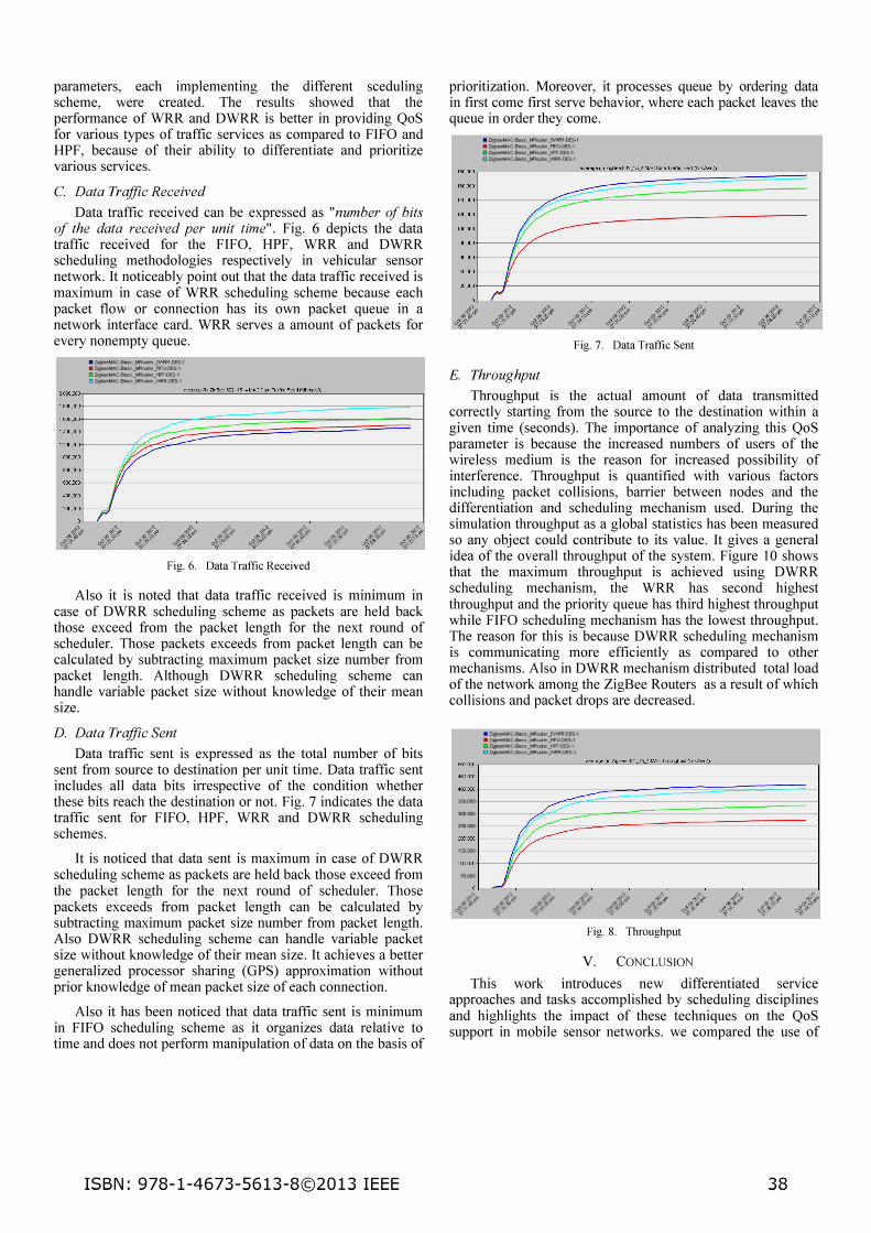
parameters, each implementing the different sceduling scheme, were created. The results showed that the performance of WRR and DWRR is better in providing QoS for various types of traffic services as compared to FIFO and HPF, because of their ability to differentiate and prioritize various services.
C. Data Traffic Received
Data traffic received can be expressed as "number of bits of the data received per unit time". Fig. 6 depicts the data traffic received for the FIFO, HPF, WRR and DWRR scheduling methodologies respectively in vehicular sensor network. It noticeably point out that the data traffic received is maximum in case of WRR scheduling scheme because each packet flow or connection has its own packet queue in a network interface card. WRR serves a amount of packets for every nonempty queue.
• Z9beeMAC-8amc_�oo.ter _CWRR-DES-l • ZgbeeMAC-8asio:U,F:oo.ter ]FO-DES-l C ZigbeeMAC-B�sic_ �oo.ter _I-FF -OES-1 o ligbeek4AC_B�"ic_�ooier _"""'.OES_1
2.0c0.(X)J,-_____ -"""·,." .. '"-"(O"'"" ... �,..'80�2-"'''- '''' MA"''' C"'''',...,.T''''''!II ffic'''R''"'''''"'"("'.,, '''�..,))'-------,
1
"BOO,COOj-------------==-
======�_1 1 "600'coo�=:::;;::;�.......--::�������1 1 .400,COOi- / / � --',ooo,cooj---/P;--h.;.-:;---.-;;:....--=----------------li
',oo),COOj--/l/-/#��---------------11
:::t===�f/��====================================�: ,OO,COO-l----,/I--------------------li
OOO,COO-l-r-;;;l}---------------------li
o�L-
_-
__ -_-_--_-_--_-_-� 1 ��� �" .,.{� �'" .,.{� dC/i .s;f�� '%'t
Fig, 6,
.,.-$� ,%'l' .,.{� dC/' .,.�1> '%� .,.'$1> �;' .,.{� d'.,� Data Traffic Received
Also it is noted that data traffic received is minimum in case of DWRR scheduling scheme as packets are held back those exceed from the packet length for the next round of scheduler. Those packets exceeds from packet length can be calculated by subtracting maximum packet size number from packet length. Although DWRR scheduling scheme can handle variable packet size without knowledge of their mean size.
D. Data Traffic Sent
Data traffic sent is expressed as the total number of bits sent from source to destination per unit time. Data traffic sent includes all data bits irrespective of the condition whether these bits reach the destination or not. Fig. 7 indicates the data traffic sent for FIFO, HPF, WRR and DWRR scheduling schemes.
It is noticed that data sent is maximum in case of DWRR scheduling scheme as packets are held back those exceed from the packet length for the next round of scheduler. Those packets exceeds from packet length can be calculated by subtracting maximum packet size number from packet length. Also DWRR scheduling scheme can handle variable packet size without knowledge of their mean size. It achieves a better generalized processor sharing (GPS) approximation without prior knowledge of mean packet size of each connection.
Also it has been noticed that data traffic sent is minimum in FIFO scheduling scheme as it organizes data relative to time and does not perform manipulation of data on the basis of
ISBN: 978-1-4673-5613-8©2013 IEEE
prioritization. Moreover, it processes queue by ordering data in first come first serve behavior, where each packet leaves the queue in order they come.
• Zi�C_�sic_�o"'er_�_DES_l • Zi�C-&lsic_�o"'erJFO-DES_l o ZigbeeMAC-&lsic_�o"'er _fff_DES.l o ZigbeeMAC-&lsic_�olier _WRR.OES_l
Fig, 7, Data Tramc Sent
E. Throughput
Throughput is the actual amount of data transmitted correctly starting from the source to the destination within a given time (seconds). The importance of analyzing this QoS parameter is because the increased numbers of users of the wireless medium is the reason for increased possibility of interference. Throughput is quantified with various factors including packet collisions, barrier between nodes and the differentiation and scheduling mechanism used. During the simulation throughput as a global statistics has been measured so any object could contribute to its value. It gives a general idea of the overall throughput of the system. Figure 10 shows that the maximum throughput is achieved using DWRR scheduling mechanism, the WRR has second highest throughput and the priority queue has third highest throughput while FIFO scheduling mechanism has the lowest throughput. The reason for this is because DWRR scheduling mechanism is communicating more efficiently as compared to other mechanisms. Also in DWRR mechanism distributed total load of the network among the ZigBee Routers as a result of which collisions and packet drops are decreased.
• ZigbeeMAC-Basic_"",,oiJ:er _D'WRR-DES-l • Zio,j:leeMAC.BMicJ,f'Olier JFO-DES-l DZio.JoeeMAC_B,,�ic-'.lRo<ief_I-ff_DES_1 o Zio'#leeMAC-B"�ic_J¥lRQlJef _fflR-DES-l
;oo,ooo,-______ =···='.,,=(O=''''"=. OO�'-'�;-= ... ='=T�"''=''''=('''='' '=�C»� _____ _____,I 450,oooj-----------------------l1
<OO 'OO)t::::=:;/
��� /"--:::::� �������:-::-:�JI 350,000
/ _____ :: ff' ----"",oooj---Itf/'7'/,y::::c--------------------j1
'",,000 --I//iY�y'--------------------__I1 ,OO,OOOj--IIfI!J'f/'----------------------l1
",,00) --JI'I------------------11 o ���---- _--_--_----__ --_----_--__ --�
.,.�1> .,.'$1> .,.'$1> .,.�1> .,.'$1> �)" �� �� r:%"t '45>' Fig, 8, Throughput
v. CONCLUSION
This work introduces new differentiated service approaches and tasks accomplished by scheduling disciplines and highlights the impact of these techniques on the QoS support in mobile sensor networks. we compared the use of
38
different quality control algorithms for prioritizing and scheduling of traffic received from vehicles in ZigBee environment. On the basis of our measurements and results, we presented that DWRR and WRR have increased QoS by decreasing the collision, packet drop rate and delay. This research can be further extended by implementing existing modern priority and scheduling mechanism or by presenting innovative new algorithm for particular scenario of vehicular sensor networks.
VI. ACKNOWLEDGEMENT.
This work is supported by the research center of the college of Computer and Information Sciences, King Saud University, under the project number RC130396.
References [I] U. Lee and M. Gerla, "Survey of urban vehicular sensing platforms",
Computer Networks, vol. 54, no.4, 2010, pp.527-544.
[2] K.C. Rahman, "A Survey on Sensor Network", Journal of Convergence Information Technology (JCIT), vol.Ol, Issue 01, 2010, pp.76-87.
[3] 1. Yick, B. Mukhe�jee, and D. Ghosal, "Wireless Sensor Network Survey", Computer Networks: The International Journal of Computer and Telecommunications Networking, vol. 52, no. 12, 2008, pp. 2292-2330.
[4]
[5]
I.F. Akyildiz, W. Su, Y. Sankarasubramaniam, and E. Cayirci, "A Survey on Sensor Networks", IEEE Communications Magazine, vol. 40, no. 8,2002,pp. 104-112.
B. Nefzi, Y.Q. Song, "QoS for wireless sensor networks: Enabling service differentiation at the MAC sub-layer using CoSenS", Ad Hoc Networks, vol. 10, no. 4, 2012, pp.680-695.
[6] T. Zhang, L. Chen, D. Chen, and L. Xie, "EEFF: A Cross-Layer Designed Energy Efficient Fast Forwarding Protocol for Wireless Sensor Networks", In the proceedings of IEEE Wireless Communications and Networking Conference (WCNC), pp. 1-6,2009.
[7] A. Koubaa, M. Alves, B. efzi, and Y.Q. Song, "Improving the IEEE 802.15.4 Slotted CSMAICA MAC for Time-Critical Events in Wireless Sensor Networks", Workshop on Real Time Networks (RTN), vol. 6, 2006.
[8] S.C. Ergen and P. Varaiya, "TDMA scheduling algorithms for wireless sensor networks", Wireless Networks, vol. 16, no. 4, 2010, pp.985-997.
[9] Q. Liu, X. Wang, and G.B. Giannakis, "A Cross-Layer Scheduling Algorithm With QoS Support in Wireless Networks", IEEE transaction on vehicular technology, vo1.55, no.3, pp.839-847, 2006.
[10] P. Papageorgiou, "Literature Survey on Wireless Sensor Networks", ACM SIGOPS Operating Systems Review, pp.6, 1999.
[11]
[12]
L. Song and D. Hatzinakos, "A Cross-Layer Architecture of Wireless Sensor Networks for Target Tracking", IEEE/ACM transaction on networking, voI.15, no.l, pp.145-158, 2007.
1. Demirkol, C. Ersoy, and F. Alagoz, "MAC Protocols for Wireless Sensor Networks: A Survey", IEEE Communications Magazine, vo1.44, no.4, pp.115-121, 2006.
[13] K. Kredo II and P. Mohapatra, "Medium Access Control in Wireless Sensor Networks", Computer Networks, vol. 51, no.4, pp.961-994, 2007.
[14] W. Ye and 1. Heidemann, "Medium Access Control in Wireless Sensor Networks", Wireless sensor networks, pp.73-91, 2004.
[15]
[16]
P. Buonadonna, D. Gay, 1.M. Hellerstein, W. Hong, and S. Madden, "TASK: Sensor Network in a Box", In Proceedings of the 2nd IEEE European Workshop on Wireless Sensor Networks and Applications (EWSN), pp.133-144, 2005.
S. Madden, M.J. Franklin, J.M. Hellerstein, and W. Hong, 'The Design of an acquisitional Query Processor for Sensor Networks", In Proceedings of International conference on Management of data ACM SIGMOD, pp.491-502, 2003.
ISBN: 978-1-4673-5613-8©2013 IEEE
[17]
[18]
[19]
[20]
W. Ye, J. Heidemann, and D. Estrin, "An Energy-Efficient MAC Protocol for Wireless Sensor Networks", In Proceedings of the IEEE Computer and Communications Societies INFOCOM, voI.3, pp. 1567-1576,2002.
LAN MAN Standards Committee of the IEEE Computer Society, "Wireless LAN medium access control (MAC) and physical layer (PHY) specification", IEEE, NY, USA, IEEE Std 802.11,1999.
M.A.Yigitel, 0.0. Incel, and C. Ersoy, "QoS-aware MAC protocols for wireless sensor networks: A survey", Computer Networks,voI.55, no.8, pp.1982-2004,2011.
1. Chen, M. Dlaz, L. L1opis, B. Rubio, and 1.M. Troya, "A survey on quality of service support in wireless sensor and actor networks: Requirements and challenges in the context of critical infrastructure protection", Journal of Network and Computer Applications, vol. 34, no. 4, pp. 1225-1239,2011.
[21] D. Chen and P.K. Varshney, "QoS Support in Wireless Sensor Networks: A Survey", International Conference on Wireless Networks, pp.227-233,2004.
[22] K. Lin, "Research on adaptive target tracking in vehicle sensor networks", Journal of Network and Computer Applications, 2012.
[23] B. Nefzi and Y.Q. Song, "QoS for wireless sensor networks: Enabling service differentiation at the MAC sub-layer using CoSenS", Ad Hoc Networks, vol. I 0, no.4, pp.680-695, 2012.
[24]
[25]
[26]
[27]
[28]
[29]
C. Annadurai, "Review of Packet Scheduling Algorithms in Mobile Ad Hoc Networks", International Journal of Computer Applications, vol. 15, no. I , pp.0975-8887, 20 II.
O. Chipara, C. Lu, and G.C. Roman, "Real-Time Query Scheduling for Wireless Sensor Networks", 28th IEEE International Real-Time Systems Symposium (RTSS), pp.389-399, 2007.
B.G. Chun and M. Baker, "Evaluation of Packet Scheduling Algorithms in Mobile Ad Hoc Networks", ACM SIGMOBILE Mobile Computing and communications Review, vol. 6, no. 3, pp. 36-49, 2002.
M.A. Yigitel, 0.0. Ince!, and C. Ersoy, "Design and implementation of a QoS-aware MAC protocol for Wireless Multimedia Sensor Networks", Computer Communications, vol.34, no.16, pp.1991-2001, 2011.
Z.J. Haas and J. Deng, "On Optimizing the Backoff Interval for Random Access Schemes", IEEE IEEE Transactions on Communications, vol. 51, no.12, pp. 2081-2090, 2003.
F. Cali, M. Conti, and E. Gregori, "IEEE 802.11 Protocol: Design and Performance Evaluation of an Adaptive Backoff Mechanism", IEEE Journal on Selected Areas in Communications, vol. 18, no.9, pp. 1774-1786,2000.
[30] F. Cali, M. Conti, E. Gregori, "Performance Modeling of an Enhanced IEEE 802.11 Protocol", In Proceedings of IFIP ATM, vo1.99, 1999.
39
Enhanced-MPR-CDS approach for self-organization and routing in
WSNs
Jihed KHASKHOUSSI 1 , Ridha OUNI
2
1 EE, Faculty of Sciences of Monastir, Tunisia
2 College of Computer and Information Sciences, King Saud University, KSA.
Abstract
Wireless sensor networks are poised to become
a very significant enabling technology in many
sectors. Already a few very low power wireless
sensor platforms have entered the marketplace.
Almost all of these platforms are designed to run on
batteries that have a very limited lifetime. Recent
advances in wireless sensor networks have led to
many new protocols specifically designed for sensor
networks where energy awareness is an essential
consideration. Most of the attention, however, has
been given to the self-organization and routing
protocols since they might differ depending on the
application and network architecture.
This work evaluates performances of two self
organization protocols: MPR and MPR-CDS in the
goal to propose new rules reducing the dominants
and relay sets. This optimization is based on the
probability of being covered by many of neighbor's
dominants. Those sets operate together to route data
from sender to receiver. We use a multi-hop routing
to reduce energy consumption and retransmission
rate.
Key words: WSN, Self-Organization, MPR, MPR-CDS.
1. Introduction
A wireless sensor network (WSN) is an
interconnected set of sensor nodes that monitor and
collect information about the environment and
transmit the collected data generally to sink node
which saves, analyzes and interprets data. Each
individual sensor node in the network consists of one
or more sensors, a radio transceiver, a
microprocessor and a small battery. During the last
decade, it has drawn extensive attention due to the
wide range of promising applications, such as
environmental monitoring, industrial sensing and
diagnostics, battlefield surveillance, target tracking,
search and rescue, and disaster relief [1, 2].
The lifetime of a network is a crucial feature in WSN
applications. Another main feature is reducing the
size of the routing table in each node. Most of the
techniques proposed, for extending the sensor
network lifetime and reducing the routing table size,
are based on hierarchical architectures or clustering
techniques [1].
The self-organization protocols are energy-
efficiently improved. They aim to select a limited set
to act as routers (active nodes) allowed message
retransmission. They avoid the blind flooding which
generates a lot of collisions that could possibly
prevent the broadcasting from being correctly
performed beside the significant energy consumption
by redundant messages. Many schemes of self
organization protocol have been proposed to replace
blind flooding, and they are classified in different
categories: simple flooding, probability based, area
based and neighbor knowledge methods.
In the present work, we are interested on the
neighbor knowledge based protocol. We aim to
optimize the Multipoint Relay-Connected Dominate
Set (MPR-CDS) scheme and propose a self enhanced
routing approach.
The paper is organized as follows. In section 2, we
present an overview of the main WSN concepts. We
also introduce and analyze the MPR-CDS self-
organization protocol. While, in section 3, we
develop and evaluate our optimized approach. Next,
section 4 describes the routing approach using an
intermediate field. Finally, section 5 provides some
remarks and concludes the paper.
2. Wireless Sensor Networks (WSN)
Primitive network is based on blind flooding
(Fig.1). The packet is retransmitted by all the
intermediate nodes in order to broadcast it in the
network. It is simple, easy to implement, and gives a
high probability that each node, which is not isolated
from the network, will receive the broadcasted
message. However, it consumes a large amount of
© ICCIT 2012 875
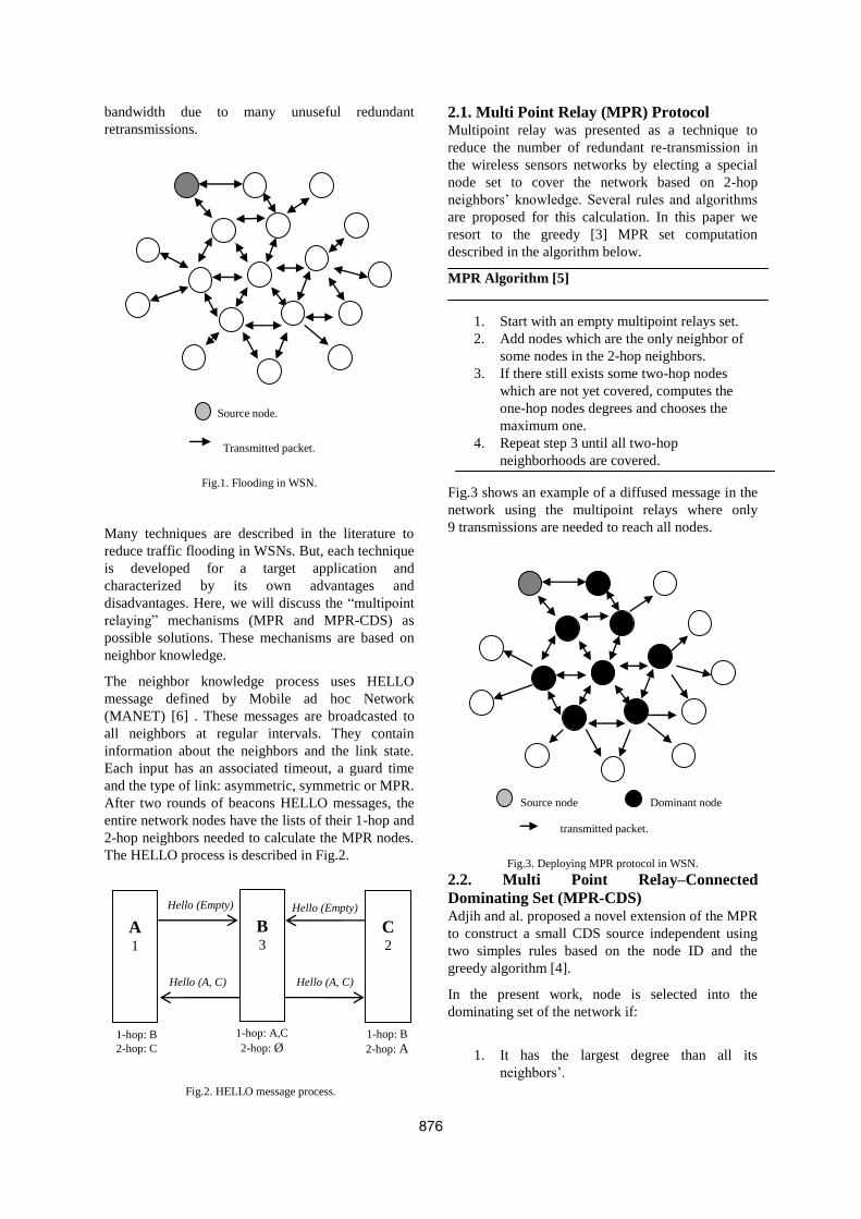
bandwidth due to many unuseful redundant
retransmissions.
Source node.
Transmitted packet.
Fig.1. Flooding in WSN.
Many techniques are described in the literature to
reduce traffic flooding in WSNs. But, each technique
is developed for a target application and
characterized by its own advantages and
disadvantages. Here, we will discuss the “multipoint
relaying” mechanisms (MPR and MPR-CDS) as
possible solutions. These mechanisms are based on
neighbor knowledge.
The neighbor knowledge process uses HELLO
message defined by Mobile ad hoc Network
(MANET) [6] . These messages are broadcasted to
all neighbors at regular intervals. They contain
information about the neighbors and the link state.
Each input has an associated timeout, a guard time
and the type of link: asymmetric, symmetric or MPR.
After two rounds of beacons HELLO messages, the
entire network nodes have the lists of their 1-hop and
2-hop neighbors needed to calculate the MPR nodes.
The HELLO process is described in Fig.2.
Fig.2. HELLO message process.
2.1. Multi Point Relay (MPR) Protocol Multipoint relay was presented as a technique to
reduce the number of redundant re-transmission in
the wireless sensors networks by electing a special
node set to cover the network based on 2-hop
neighbors’ knowledge. Several rules and algorithms
are proposed for this calculation. In this paper we
resort to the greedy [3] MPR set computation
described in the algorithm below.
MPR Algorithm [5]
1. Start with an empty multipoint relays set.
2. Add nodes which are the only neighbor of
some nodes in the 2-hop neighbors.
3. If there still exists some two-hop nodes
which are not yet covered, computes the
one-hop nodes degrees and chooses the
maximum one.
4. Repeat step 3 until all two-hop
neighborhoods are covered.
Fig.3 shows an example of a diffused message in the
network using the multipoint relays where only
9 transmissions are needed to reach all nodes.
Source node Dominant node
transmitted packet.
Fig.3. Deploying MPR protocol in WSN.
2.2. Multi Point Relay–Connected
Dominating Set (MPR-CDS) Adjih and al. proposed a novel extension of the MPR
to construct a small CDS source independent using
two simples rules based on the node ID and the
greedy algorithm [4].
In the present work, node is selected into the
dominating set of the network if:
1. It has the largest degree than all its
neighbors’.
A 1
B 3
C 2
Hello (Empty) Hello (Empty)
Hello (A, C) Hello (A, C)
1-hop: A,C
2-hop: Ø
1-hop: B
2-hop: A
1-hop: B
2-hop: C
876
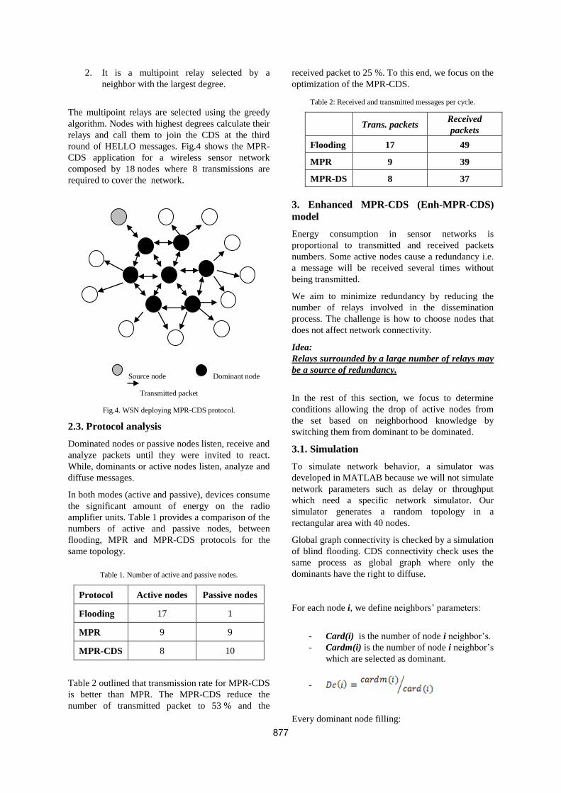
2. It is a multipoint relay selected by a
neighbor with the largest degree.
The multipoint relays are selected using the greedy
algorithm. Nodes with highest degrees calculate their
relays and call them to join the CDS at the third
round of HELLO messages. Fig.4 shows the MPR-
CDS application for a wireless sensor network
composed by 18 nodes where 8 transmissions are
required to cover the network.
Source node Dominant node
Transmitted packet
Fig.4. WSN deploying MPR-CDS protocol.
2.3. Protocol analysis
Dominated nodes or passive nodes listen, receive and
analyze packets until they were invited to react.
While, dominants or active nodes listen, analyze and
diffuse messages.
In both modes (active and passive), devices consume
the significant amount of energy on the radio
amplifier units. Table 1 provides a comparison of the
numbers of active and passive nodes, between
flooding, MPR and MPR-CDS protocols for the
same topology.
Table 1. Number of active and passive nodes.
Protocol Active nodes Passive nodes
Flooding 17 1
MPR 9 9
MPR-CDS 8 10
Table 2 outlined that transmission rate for MPR-CDS
is better than MPR. The MPR-CDS reduce the
number of transmitted packet to 53 % and the
received packet to 25 %. To this end, we focus on the
optimization of the MPR-CDS.
Table 2: Received and transmitted messages per cycle.
Trans. packets Received
packets
Flooding 17 49
MPR 9 39
MPR-DS 8 37
3. Enhanced MPR-CDS (Enh-MPR-CDS)
model
Energy consumption in sensor networks is
proportional to transmitted and received packets
numbers. Some active nodes cause a redundancy i.e.
a message will be received several times without
being transmitted.
We aim to minimize redundancy by reducing the
number of relays involved in the dissemination
process. The challenge is how to choose nodes that
does not affect network connectivity.
Idea:
Relays surrounded by a large number of relays may
be a source of redundancy.
In the rest of this section, we focus to determine
conditions allowing the drop of active nodes from
the set based on neighborhood knowledge by
switching them from dominant to be dominated.
3.1. Simulation
To simulate network behavior, a simulator was
developed in MATLAB because we will not simulate
network parameters such as delay or throughput
which need a specific network simulator. Our
simulator generates a random topology in a
rectangular area with 40 nodes.
Global graph connectivity is checked by a simulation
of blind flooding. CDS connectivity check uses the
same process as global graph where only the
dominants have the right to diffuse.
For each node i, we define neighbors’ parameters:
- Card(i) is the number of node i neighbor’s.
- Cardm(i) is the number of node i neighbor’s
which are selected as dominant.
-
Every dominant node filling:
877
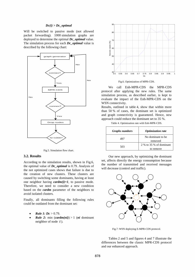
Dc(i) > Dc_optimal
Will be switched to passive mode (not allowed
packet forwarding). 1000 simulation graphs are
deployed to determine the optimal Dc_optimal value.
The simulation process for each Dc_optimal value is
described by the following chart:
graph generator
connex?
MPR-CDS
connex?
Drop nodes
N=1000?
Yes
Yes
No
No
No
Fig.5. Simulation flow chart.
3.2. Results
According to the simulation results, shown in Fig.6,
the optimal value of Dc_optimal is 0.79. Analysis of
the not optimized cases shows that failure is due to
the creation of new clusters. These clusters are
caused by switching some dominants, having at least
one neighbor having cardm(i)=1, to passive mode.
Therefore, we need to consider a new condition
based on the cardm parameter of the neighbors to
avoid isolated clusters.
Finally, all dominants filling the following rules
could be outdated from the dominant set:
Rule 1: Dc > 0.79.
Rule 2: min (cardm(ni)) > 1 (ni dominant
neighbor of node i ).
0.5 0.55 0.6 0.65 0.7 0.75 0.8 0.85 0.9 0.95 130
40
50
60
70
80
90
Dc
Succes c
ases (
%)
Fig.6. Optimization of MPR-CDS.
We call Enh-MPR-CDS the MPR-CDS
protocol after applying the new rules. The same
simulation process, as described earlier, is kept to
evaluate the impact of the Enh-MPR-CDS on the
WSN connectivity.
Results, outlined in table 4, show that within more
than 50 % of cases, the dominant set is optimized
and graph connectivity is guaranteed. Hence, new
approach could reduce the dominant set to 35 %.
Table 4. Optimization rate with Enh-MPR-CDS.
Graphs numbers Optimization rate
497 No dominant to be
removed
503 2 % to 35 % of dominant
to remove
Our new approach, by optimizing the dominant
set, affects directly the energy consumption because
the number of transmitted and received messages
will decrease (control and traffic).
Fig.7: WSN deploying E-MPR-CDS protocol.
Tables 2 and 5 and figures 4 and 7 illustrate the
differences between the classic MPR-CDS protocol
and our enhanced approach.
878
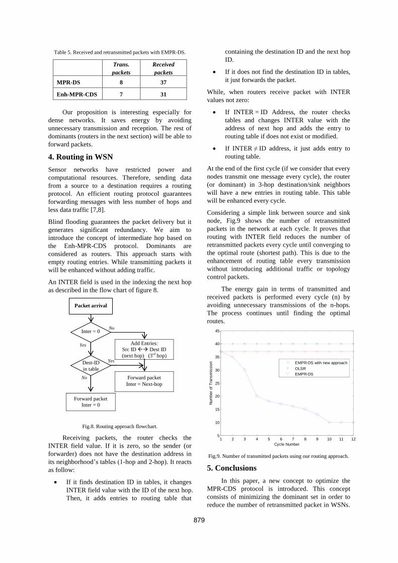
Table 5. Received and retransmitted packets with EMPR-DS.
Trans.
packets
Received
packets
MPR-DS 8 37
Enh-MPR-CDS 7 31
Our proposition is interesting especially for
dense networks. It saves energy by avoiding
unnecessary transmission and reception. The rest of
dominants (routers in the next section) will be able to
forward packets.
4. Routing in WSN
Sensor networks have restricted power and
computational resources. Therefore, sending data
from a source to a destination requires a routing
protocol. An efficient routing protocol guarantees
forwarding messages with less number of hops and
less data traffic [7,8].
Blind flooding guarantees the packet delivery but it
generates significant redundancy. We aim to
introduce the concept of intermediate hop based on
the Enh-MPR-CDS protocol. Dominants are
considered as routers. This approach starts with
empty routing entries. While transmitting packets it
will be enhanced without adding traffic.
An INTER field is used in the indexing the next hop
as described in the flow chart of figure 8.
Fig.8. Routing approach flowchart.
Receiving packets, the router checks the
INTER field value. If it is zero, so the sender (or
forwarder) does not have the destination address in
its neighborhood’s tables (1-hop and 2-hop). It reacts
as follow:
If it finds destination ID in tables, it changes
INTER field value with the ID of the next hop.
Then, it adds entries to routing table that
containing the destination ID and the next hop
ID.
If it does not find the destination ID in tables,
it just forwards the packet.
While, when routers receive packet with INTER
values not zero:
If INTER = ID Address, the router checks
tables and changes INTER value with the
address of next hop and adds the entry to
routing table if does not exist or modified.
If INTER ≠ ID address, it just adds entry to
routing table.
At the end of the first cycle (if we consider that every
nodes transmit one message every cycle), the router
(or dominant) in 3-hop destination/sink neighbors
will have a new entries in routing table. This table
will be enhanced every cycle.
Considering a simple link between source and sink
node, Fig.9 shows the number of retransmitted
packets in the network at each cycle. It proves that
routing with INTER field reduces the number of
retransmitted packets every cycle until converging to
the optimal route (shortest path). This is due to the
enhancement of routing table every transmission
without introducing additional traffic or topology
control packets.
The energy gain in terms of transmitted and
received packets is performed every cycle (n) by
avoiding unnecessary transmissions of the n-hops.
The process continues until finding the optimal
routes.
1 2 3 4 5 6 7 8 9 10 11 125
10
15
20
25
30
35
40
45
Cycle Number
Num
ber
of
Tra
nsm
issio
n EMPR-DS with new approach
OLSR
EMPR-DS
Fig.9. Number of transmitted packets using our routing approach.
5. Conclusions
In this paper, a new concept to optimize the
MPR-CDS protocol is introduced. This concept
consists of minimizing the dominant set in order to
reduce the number of retransmitted packet in WSNs.
Packet arrival
Inter = 0
Yes
No
Forward packet
Inter = Next-hop
Add Entries: Src ID Dest ID
(next hop) (3rd hop)
Dest-ID
in table
No
Forward packet
Inter = 0
Yes
879
Our new protocol, Enh-MPR-CDS, was simulated in
differents scenarios and compared to MPR and
MPR-CDS. Results confirm that a significant
amount of dominants may be removed while
connectivity still guarantee. The new protocol is
more efficient for dense networks that are composed
by hundreds or even thousands nodes.
Furthermore, a new approach for routing in
WSNs has been described. This approach deploys an
intermediate field including the router ID which
serves the destination. This approach enhances
neighbors lists (3 hops and more) without adding
traffic. Based on simulation results, it performs
routes until finding the shortest path.
References
[1] Fangting Sun and Shayman, Mark,Prolonging
Network Lifetime via Partially Controlled Node
Deployment and Adaptive Data Propagation in
WSN, Information Sciences and Systems, 2007.
CISS '07. 41st , 2007, Page(s): 226 – 231.
[2] Wei Peng and Xi-Cheng Lu. On the reduction
of broadcast redundancy in mobile adhoc
networks. In Proc. First Annual Workshop on
Mobile and AdHoc Networking and Computing,
August 11-2000, pages 129–130.
[3] Yongsheng Fu, Xinyu Wang, Wei Shi and
Shanping Li, Connectivity based greedy
algorithm with multipoint relaying for mobile
ad hoc networks, The 4th international
conference on mobile ad-hoc ans sensor
network, 2008.
[4] Cedric Adjih, philipe Jacquet and Laurent
Viennot, Computing connected dominated sets
with multipoint relays, Technical report,
INRIA, Oct.2002, www.inria.fr/rrrt/rr-
4597.html.
[5] C. Bettestetter, On the minimum node degree
and connectivity of a wireless multihop
network, in Proc. ACM MobiHoc, Lausanne,
Switzerland, Jun. 2002.
[6] T.Claussen, P.Jacquet, C. Adjih, A. Laouiti, P.
Minet,P. Muhlethaler,A. Quayyam and L.
Viennot, Optimized link state routing
protocol(OLSR), RFC 3626, Oct. 2003,
Network Working Group.
[7] I. Akyildiz,W. Su, Y. Sankarasubramaniam,
and E. Cayirci, A survey on sensor networks
Communications Magazine, IEEE, vol.40,
pp.102-114,Aug2002.
[8] K. Akkaya and M. Younis, A survey on routing
protocols for wireless sensor networks AdHoc
Networks, vol.3, no.3, pp .325-349, 2005.
880
Abstract—Nowadays, several positioning systems are
available for outdoor localization, such as the global positioning system (GPS), assisted GPS (A-GPS), and other techniques working on cellular networks, for example, Time of Arrival (TOA), Angle of Arrival (AOA) and Time Difference of Arrival (TDOA).However, with the increasing use of mobile computing devices and an expansion of wireless local area networks (WLANs), there is a growing interest in indoor wireless positioning systems based on the WLAN infrastructure. Wireless positioning systems (WPS) based on this infrastructure can be used for outdoor / indoor localization to determine the position of mobile users. An important factor in achieving this is to minimize and simplify the instructions that the mobile station (MS) has to execute in the location determination process. Finding an effective location estimation technique to facilitate processing data is the main focuses in this paper. Therefore, in the wireless propagation environment the Received Signal Strength (RSS) information from three base stations (BSs) are recorded and processed and they can provide an overlapping coverage area of interest. Then an easy new geometric technique is applied in order to effectively calculate the location of the desired MS.
Our new positioning method design was verified at the algorithmic level using Matlab tool, described in Very-high-speed integrated circuit Hardware Description Language (VHDL) at the register transfer level (RTL) and it has been synthesized using 7.1 version of FPGA Advantage for HDL Design that evaluates the circuit in terms of speed, area and power consumption.
Index Terms—Geometric technique, Position estimation, Wireless LAN, VHDL.
I. INTRODUCTION
Recently, the subject of mobile positioning in wireless communication systems has drawn considerable attention. With accurate location estimation, a variety of new applications and services such as Enhanced-911, location sensitive billing, improved fraud detection, intelligent
Monji Zaidi, Jamila Bhar and Rached Tourki are with Electronic and Micro-Electronic Laboratory (EµE, IT-06).FSM, Monastir, Tunisia
Ridha Ouni is with College of Computer and Information Sciences (CCIS), King Saud University Riyadh, KSA
transport system (ITS) and improved traffic management will become feasible [1]. Mobile positioning using radiolocation techniques usually involves time of arrival (TOA), time difference of arrival (TDOA), angle of arrival (AOA), signal strength (SS) measurements or some combination of these methods.
All of these methods are mainly based on trigonometric computation. Comparisons and survey of these methods are given in [2] and [3].
The TOA technique determines the MS position based on the intersection of three circles. Two range measurements provide an ambiguous fix, and three measurements determine a unique position.
Given the coordinates of BSj, (j = 1, 2, 3) as (Xj, Yj), and the distances dj between MS and BSj, the simplest geometrical algorithm for TOA positioning (Figure. 1(a)) is given in [2]. Coordinates of MS position (x,y) relative to BS1 can be calculated as:
���� = 12 � � � ��� + � + � + �� − �
+ � + �� − � � The simplest geometrical algorithm for TDOA
positioning (Figure. 1(b)) is given in [4]. There are two estimated TDOA-s dj, 1 between BS1 and the jth base station (j = 2, 3). Coordinates of MS position (x, y) relative to BS1 can be calculated in terms of d1 as:
���� = − � � � ��� ∗ ���,�� ,�� �� + 12 ��,� − � + ��
� ,� − � + ����
Where:
�� = � + ��
� = + �
� = + � The AOA technique determines the MS position (x, y)
based on triangulation, as shown in (Figure. 1(c)). The intersection of two directional lines of bearing with angles θ� and θ defines a unique position, each formed by a radial from a BS to the MS. The simplest geometric
Monji ZAIDI, Ridha OUNI, Jamila Bhar and Rached TOURKI
A Novel Positioning Technique with Low Complexity in Wireless LAN:
Hardware implementation
Proceedings of the World Congress on Engineering 2011 Vol II WCE 2011, July 6 - 8, 2011, London, U.K.
ISBN: 978-988-19251-4-5 ISSN: 2078-0958 (Print); ISSN: 2078-0966 (Online)
WCE 2011
solution can be derived using [5] with two AOA measurements θ� and θ:
x = Y − Y� + X�tan(θ�) − Xtan (θ)tan(θ�) − tan (π − θ)
y = Y� + (x − X�)tan(θ)
BS1 BS2
BS3 MS
Hyperbola 1
Hyperbola 2
d 1 d 2
d 3
(b)
BS1
BS3
BS2
d 1 d 2
d 3
MS
(a)
BS1 BS2
MS
2θ1θ
(c)
Fig. 1. Position determination techniques: (a) TOA; (b) TDOA; (c) AOA
Using any of the mentioned methods, the calculation can be done either at the BS [network-based schemes] or at the MS [mobile-based schemes]. Network-based schemes have high network cost and low accuracy [3]. Mobile-based location schemes are more interesting. However, since the MS has limited energy source, in the form of the battery pack, energy consumption should be minimized. An important factor in achieving this is to minimize and simplify the instructions that the MS has to execute in the location determination process. The conventional algorithms use complex computation methods that needed relatively long execution time.
In this paper, we propose a novel wireless positioning technique based on the WLAN infrastructure. The main motivation for our approach is twofold: to improve the accuracy of the location estimation and to minimize and simplify the instructions that the mobile station (MS) has to execute in the location determination process.
II. RELATED WORK
To improve the accuracy of the indoor positioning system, several techniques demonstrate the viability of this approach. Youssef et al. [6] show that the RADAR system can be improved using the perturbation technique (joint clustering technique) to handle the small-scale variations problem. This technique can improve theRADARsystem and provide location accuracy up to 3m.
The triangulation mapping interpolation system (CMU-TMI) [7] performs a location calculation on the current data, interpolates that data with the information in the database, and then returns a location estimate based on this interpolation. However, power consumption increases to measure the signal strength on the client side.
The Ekahau Positioning Engine 4.0 [8], released in October 2006, also uses an IEEE 802.11 network to provide location information. It achieves an average
accuracy of 1m with at least three audible channels in each location. This system requires site calibration up to 1 h per 1,200m2. While calibration-based efforts present good accuracy results, there is still room for performance enhancements. Due to the very dynamic nature of the RF signal, the assumption that the radio map built in the calibration phase remains consistent to the measurements performed in the real-time phase does not hold in practice; thus, at times, there is a need to rebuild the radio map. It seems more reasonable to design a fully-automatic system capable of acknowledging RSSI characteristics and variations in both spatial and time domains.
Hitachi [9] released location technology based on TDOA in March 2005. This system uses two types of access points: a Master AP and a Slave AP. Slave APs synchronize their clocks with that of a Master AP and measure the arrival time from a mobile terminal; the Master AP determines the location of the mobile terminal using the TDOA between the signal reception times at multiple Slave APs. While this technique has been found to achieve good results in indoor environments, it requires specialized hardware and fine-grain time synchronization, which increases the cost of this type of solution.
Kanaan proposed a closest-neighbor with TOA grid algorithm (CN-TOAG) [10]. This geolocation algorithm presents a TDOA-based position detection technique to improve location accuracy in the indoor environment by estimating the location of the user as the grid point. This technique is similar to the previous one [11], as it needs specialized hardware and fine grain time synchronization, which increase costs.
III. NEW GEOMETRIC LOCATION ALGORITHM
BASED ON THREE BSS
In the general geometrical triangulation location researches, they assumed that the measured noise is additive and the NLOS error is a large positive bias which causes the measured ranges to be greater than the true ranges [12].
BS1 BS2
BS3
A B
C
Fig. 2. Measured range circles and the associated intersected area
Under the assumption, the MS location will guarantee to lie in the overlapped region (enclosed by points A, B and C) of the range circles as shown in Figure. 2. Thus the MS
Proceedings of the World Congress on Engineering 2011 Vol II WCE 2011, July 6 - 8, 2011, London, U.K.
ISBN: 978-988-19251-4-5 ISSN: 2078-0958 (Print); ISSN: 2078-0966 (Online)
WCE 2011
is necessarily located in the region formed by the points BS1, BS2 and BS3. But, it is noted that the intersection of three circles may not be overlapped with the real measurement results. Therefore, with the above assumption we have to judge whether the three circles intersect or not in our location algorithm.
If circles intersect as depicted in Figure. 3, then three triangles can be drawn as: BS1MSBS2, BS2MSBS3 and BS3MSBS1. Assumptions:
• Different BSs are placed (two to two) at an equal distance
• The coordinates of BSs are known by the MS
• The MS can inquire only on the received power coming from the BSs (i.e. the distance which separates it from each BS).
• d� + d > (; d + d > ( *+� d + d� > (
BS1 BS2
BS3
MS d1 d2
d3
23θ
21θ12θ
13θ
32θ31θ
),( 12120 yxA
),( 23230 yxB),( 31310 yxC
D
r1
Fig. 3. The associated triangles of the standard intersection of three circles.
Note by: • D: The distance between tow BSs.
• A0, B0 and C0 are the orthogonal projections of the MS on (BS1 BS2), (BS2, BS3) and (BS3 BS1) respectively.
• d1, d2 and d3 are the distances that separate the MS from BS1, BS2 and BS3 respectively.
• θ12: is the geometrical angle between the MS-BS1 and BS1-BS2. (Same things for the other angles).
We focus firstly on the triangle BS1MSBS2. Based on the above assumptions and figure 2, we can write.
r� = d�cosθ� We can also write
d = (D − r�) + (d� − r�) ⟹
d = (D − d�cosθ�) + (d� − d�cosθ�) ⟹
d = D + d� − 2Dd�cosθ� = D + d� − 2Dr� ⟹
r� = D + d� − d2D
We define here the first factor q�by
q� = r�D = D + d� − d2D
Coordinates (x�, y�) of the point A0 are given in [13] by
x� = q�X + (1 − q�)X� y� = q�Y + (1 − q�)Y� Where:
(X�, Y�) and (X, Y) are the coordinates of BS1 and BS2, respectively.
Let the distance between BS2 and B0 be r and the distance between BS3 and C0 be r As we described previously, we can get the coordinates of points B0 and C0 as:
x = qX + (1 − q)X y = qY + (1 − q)Y x � = q X� + (1 − q )X y � = q Y� + (1 − q )Y Where:
q = rD = D + d − d 2D
q = r D = D + d − d�2D
MS is then located in a new triangle A0B0C0, which is smaller in terms of area compared to the starting triangle BS1BS2BS3. In the other word we have just created three
new virtual BSs placed at A0, B0 and C0. It is very easy to calculate the distances between the MS and the new points A0, B0 and C0 using the Pythagoras formula. Thus
d(MS, A6) = 7d� − r�
d(MS, B6) = 7d − r
d(MS, C6) = 7d − r
Now, with the three new virtual BSs, MS can repeat the same calculations as shown above. During this second iteration, the orthogonal projections of MS on (A0B0), (B0C0) and (C0A0) must be done to obtain new point A1, B1 and C1 that their coordinates may be determined as previously. A1B1C1‘s area is smaller than the A0B0C0 one. At the i;< iteration, the MS will be located in an AiBiCi triangle which is smaller than Ai-1Bi-1Ci-1 one. This AiBiCi triangle allows to designing the next triangle Ai+1Bi+1Ci+1.
Proceedings of the World Congress on Engineering 2011 Vol II WCE 2011, July 6 - 8, 2011, London, U.K.
ISBN: 978-988-19251-4-5 ISSN: 2078-0958 (Print); ISSN: 2078-0966 (Online)
WCE 2011
After a small number of iterations, the coordinates of three vertices of the triangle (A, B and C) converge to the actual coordinates of the MS. At the limit, the triangle AconvBconvCconv with vertices Aconv, Bconv and Cconv will be considered as a point. So, it is possible to write: x=>?@A ≈ xC>?@A ≈ xD>?@A
y=>?@A ≈ yC>?@A ≈ yD>?@A
We can then take the coordinates of the MS as:
xEF = x=>?@A + xC>?@A + xD>?@A3
yEF = y=>?@A + yC>?@A + yD>?@A3
The division by 3 implies that the MS is equivalent to the gravity center of the Aconv, Bconv Cconv triangle.
Figure 8 (section 5) shows the evolution and the convergence of the three vertices coordinates for different values of di (d1, d2 and d3).
IV. VHDL MODEL
The operation destined to calculate the coordinates of a mobile terminal is known as a Location Process. Original design of this process, has just considered.
Figure 4 shows the main elements involved in our new mechanism: the MS, Three BSs, and the distribution system (DS) or Ethernet.
It can mentioned that different BSs are placed (Two to two) at an equal distance, and the MS can inquire only on the position and the received time coming from the BSs (i.e. the distance which separates it from each BS)
The equations for the x and y position of the mobile was modeled using VHDL. The numeric_std package was used to construct the VHDL model that was readily synthesized into a low power digital circuit. The input signal of the model are the x, y positions of the three BSs, i,j,k in meters, and the signals TOA from the individual BS to the mobile in nanoseconds. The input signal assignments are xi, yi, TOAi, xj, yj, TOAj, xk, yk, TOAk
Fig. 4. Involved elements in the Positioning process
Now, we describe the hardware implementation of the location process. Figure 5 illustrates the system architecture; we try to divide location process to 4 parts: a process location algorithm, the square root component, divider block and buffers to store data. The following notations are used to describe the signal type: I: input signal; O: output signal
TABLE I PROCESS LOCATION PART INTERFACE SIGNALS
Name Type Description CK I:bit Operation clock. RST I:bit RESET system TOA1 I:std_logic_vector Input from the BS1, it gives the time of
arrival value to travel the d1distance X1 I:std_logic_vector BS1 abscissa Y1 I:std_logic_vector BS1ordinate TOA2 I:std_logic_vector Input from the BS2, it gives the time of
arrival value to travel the d2 distance. X2 I:std_logic_vector BS2 abscissa Y2 I:std_logic_vector BS2abscissa TOA2 I:std_logic_vector Input from the BS3, it gives the time of
arrival value to travel the d3 distance. X3 I:std_logic_vector BS3 abscissa Y3 I:std_logic_vector BS3 abscissa Xestim O:
std_logic_vector Estimated abscissa of MS
Yestim O: std_logic_vector
Estimated ordinate of MS
First, the main program (process location) receives data
from the external environment. Then, it calculates the parameters r�, q� , r, q, r , and q as it was presented in Section 3. During this stage the divider component is called by the main program to perform the operations division. Meanwhile the virtual coordinates (x�, y�), (x , y ) and (x �, y �) of points A0, B0 and C0
respectively, are determined.
Secondly, the distances d(MS, A6), d(MS, B6) and d(MS, C6) are calculated using the square root operators
Fig. 5. Top level structure of the Location circuit
The implemented square root algorithm uses unsigned
integers, which have several advantages over floating-point
Proceedings of the World Congress on Engineering 2011 Vol II WCE 2011, July 6 - 8, 2011, London, U.K.
ISBN: 978-988-19251-4-5 ISSN: 2078-0958 (Print); ISSN: 2078-0966 (Online)
WCE 2011
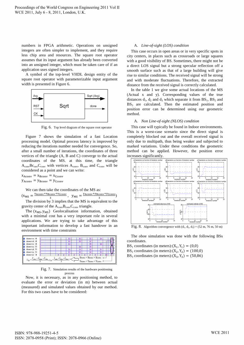
numbers in FPGA arithmetic. Operations on unsigned integers are often simpler to implement, and they require less chip area and resources. The square root operator assumes that its input argument has already been converted into an unsigned integer, which must be taken care of if an application uses signed integers.
A symbol of the top-level VHDL design entity of the square root operator with parameterizable input argument width is presented in Figure 6.
Fig. 6. Top level diagram of the square root operator
Figure 7 shows the simulation of a fast Location
processing model. Optimal process latency is improved by reducing the iterations number needed for convergence. So, after a small number of iterations, the coordinates of three vertices of the triangle (A, B and C) converge to the actual coordinates of the MS. at this time, the triangle AconvBconvCconv with vertices Aconv, Bconv and Cconv will be considered as a point and we can write: x=>?@A = xC>?@A = xD>?@A y=>?@A = yC>?@A = yD>?@A
We can then take the coordinates of the MS as:
(xEF = HIJKLMNHOJKLMNHPJKLM , yEF = QIJKLMNQOJKLMNQPJKLM
)
The division by 3 implies that the MS is equivalent to the gravity center of the AconvBconvCconv triangle. The (xEF, yEF) Geolocalisation information, obtained with a minimal cost has a very important role in several applications. We are trying to take advantage of this important information to develop a fast handover in an environment with time constraints
Fig. 7. Simulation results of the hardware positioning process
Now, it is necessary, as in any positioning method, to evaluate the error or deviation (in m) between actual (measured) and simulated values obtained by our method. For this two cases have to be considered:
A. Line-of-sight (LOS) condition
This case occurs in open areas or in very specific spots in city centers, in places such as crossroads or large squares with a good visibility of BS. Sometimes, there might not be a direct LOS signal but a strong specular reflection off a smooth surface such as that of a large building will give rise to similar conditions. The received signal will be strong and with moderate fluctuations. Therefore, the extracted distance from the received signal is correctly calculated.
In the table 1 we give some actual locations of the MS (Actual x and y). Corresponding values of the true distances d1, d2 and d3 which separate it from BS1, BS2 and BS3 are calculated. Then the estimated position and position error can be determined using our geometric method.
A. Non Line-of-sight (NLOS) condition
This case will typically be found in Indoor environments. This is a worst-case scenario since the direct signal is completely blocked out and the overall received signal is only due to multipath, thus being weaker and subjected to marked variations. Under these conditions the geometric method can be applied. However, the position error increases significantly.
Fig. 8. Algorithm convergence with (d1, d2, d3) = (52 m, 76 m, 50 m)
The oboe simulation was done with the following BSs
coordinates. BS1 coordinates (in meters):(X�, Y�) = (0,0) BS2 coordinates (in meters):(X, Y) = (100,0) BS3 coordinates (in meters):(X , Y ) = (50,86)
0 5 10 15 2030
40
50
60x(A)variations as function of iterations number
iterations number
x(A
)
0 5 10 15 2020
40
60
80x(B)variations as function of iterations number
iterations number
x(B
)
0 5 10 15 2025
30
35
40x(C)variations as function of iterations number
iterations numbers
x(C
)
0 5 10 15 200
20
40
60y(A)variations as function of iterations number
iterations numbers
y(A
)
0 5 10 15 2030
40
50
60y(B)variations as function of iterations number
iterations number
y(B
)
0 5 10 15 2030
35
40
45y(C)variations as function of iterations number
iterations number
y(C
)
0 5 10 15 2030
35
40
45 estimated abscissa of MS
iterations number
x(M
S)
0 5 10 15 2030
35
40 estimated ordinate of MS
iterations number
y(M
S)
Proceedings of the World Congress on Engineering 2011 Vol II WCE 2011, July 6 - 8, 2011, London, U.K.
ISBN: 978-988-19251-4-5 ISSN: 2078-0958 (Print); ISSN: 2078-0966 (Online)
WCE 2011
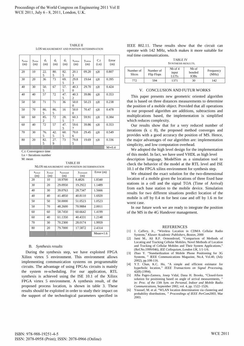
TABLE II LOS MEASUREMENT AND POSITION DETERMINATION
xactua (m)
yactua (m)
d1
(m)
d2
(m)
d3
(m)
xestima (m)
yestima (m)
C.t (i.n)
Error (m)
20 10 22.5
80.5
82.5
20.13
09.20 ≤8 0.807
30 20 36 73 69.5
29.83
19.64 ≤8 0.395
40 30 50.5
67 57.5
40.30
29.70 ≤8 0.424
40 40 57 72 47.5
40.32
39.86 ≤8 0.353
50 50 71 71 36 50.00
50.23 ≤8 0.238
50 70 86.5
86.5
16 50.00
70.47 ≤8 0.478
60 60 85.2
72 28.5
60.37
59.91 ≤8 0.384
60 40 72 57 47.5
59.67
39.86 ≤8 0.353
70 30 76.5
42.5
60.5
70.06
29.45 ≤8 0.549
80 20 82.5
27.9
73 79.85
19.69 ≤8 0.336
M≈0.4 C.t: Convergence time I.n = Iterations number M: mean
TABLE III NLOS MEASUREMENT AND POSITION DETERMINATION
xactual (m)
yactual
(m) xestimated
(m) yestimated
(m) Error (m)
20 10 18.9700 8.4826 1.8340
30 20 29.0950 19.2922 1.1489
40 30 39.0763 28.7347 1.5666
40 40 41.4850 40.8110 1.6920
50 50 50.0000 51.0523 1.0523
50 70 48.2600 70.9884 2.0011
60 60 58.7450 60.6642 1.4199
60 40 61.1350 40.4331 1.2148
70 30 70.2300 28.0174 1.9959
80 20 79.7000 17.5872 2.4314
Mean≈1.6
B. Synthesis results During the synthesis step, we have exploited FPGA
Xilinx virtex 5 environment. This environment allows implementing communication systems on programmable circuits. The advantage of using FPGAs circuits is mainly the system re-scheduling. For our application, RTL synthesis is achieved using the ISE 10.1 of the Xilinx FPGA virtex 5 environment. A synthesis result, of the proposed process location, is shown in table 3. These results should be exploited in order to study their impact on the support of the technological parameters specified in
IEEE 802.11. These results show that the circuit can operate with 142 MHz, which makes it more suitable for real time communications.
TABLE IV SYNTHESIS RESULTS.
Number of Slices
Number of Flip Flops
Nb of 4 input LUTs
Nb of bonded IOBs
Frequency (MHz)
772 594 1371 30 142
V. CONCLUSION AND FUTUR WORKS
This paper presents new geometric oriented algorithm that is based on three distances measurements to determine the position of a mobile object. Provided that all operations in our proposed algorithm are additions, subtractions and multiplications based, the implementation is simplified which reduces complexity.
Our results show that for a very reduced number of iterations (k ≤ 8), the proposed method converges and provides with a good accuracy the position of MS. Hence, the major advantages of our algorithm are: implementation simplicity, and low computation overhead.
We adopted the high level design for the implementation of this model. In fact, we have used VHDL as high level description language, ModelSim as a simulation tool to check the behavior of the model at the RTL level and ISE 10.1 of the FPGA xilinx environment for synthesis step.
We obtained the exact solution for the two-dimensional location of a mobile given the locations of three fixed base stations in a cell and the signal TOA (Time of Arrival) from each base station to the mobile device. Simulation results for two different situations predict location of the mobile is off by 0.4 m for best case and off by 1.6 m for worst case.
In our future work we are ready to integrate the position of the MS in the 4G Handover management.
REFERENCES [1] J. Caffery, Jr., “Wireless Location in CDMA Cellular Radio
Systems,” Kluwer Academic Publishers, Boston, 2000 [2] Jami M., Ali R.F. Ormondroyd, “Comparison of Methods of
Locating and Tracking Cellular Mobiles, Novel Methods of Location and Tracking of Cellular Mobiles and Their System Applications,” (Ref.No.1999/046), IEE Colloquium, London UK, 1/1-1/6.
[3] Zhao Y. “Standardization of Mobile Phone Positioning for 3G Systems, ” IEEE Communications Magazine, No.4, Vol.40, (July 2002), pp.108-116.
[4] Y.T. Chan, K.C. Ho, “A simple and efficient estimator for hyperbolic location,” IEEE Transactions on Signal Processing, 42(8) (1994).
[5] Alba Pages-Zamora, Josep Vidal, Dana H. Brooks, “Closed-form solution for positioning based on angle of arrival measurements, ” in: Proc. of the 13th Sym. on Personal, Indoor and Mobile Radio Communications, September 2002, vol. 4, pp. 1522–1526.
[6] Youssef, M. et al. “WLAN location determination via clustering and probability distributions, ” Proceedings of IEEE PerCom2003, Mar 2003.
Proceedings of the World Congress on Engineering 2011 Vol II WCE 2011, July 6 - 8, 2011, London, U.K.
ISBN: 978-988-19251-4-5 ISSN: 2078-0958 (Print); ISSN: 2078-0966 (Online)
WCE 2011
[7] Smailagic, A., & Kogan, D. (2002). Location sensing and privacy in a context-aware computing environment,” IEEE Wireless Communications, 9(5), 10–17, Oct 2002.
[8] Ekahau, Inc., “Ekahau Positioning Engine 4.0”, http://www.ekahau.com/. Accessed, Oct 2006.
[9] Yamasaki, R. et al. (2005), “ TDOA location system for IEEE 802.11b WLAN, ” Proceedings of IEEE WCNC’05, pp. 2338–2343, March 2005.
[10] Kanaan, M., & Pahlavan, K. (2004). CN-TOAG: , “A new algorithm for indoor geolocation, ” Proceedings of IEEE PIMRC’04, 3, 1906–1910, Sep 2004.
[11] Biacs, Z., Marshall, G., Meoglein, M., & Riley, W. (2002). “The qualcomm/SnapTrack wireless-assisted GPS hybrid positioning system and results from initial commercial deployments,” Proceedings of IOS GPS, pp. 378–384, 2002.
[12] C. D. Wann and H.C. Chin, “Hybrid TOA/RSSI Wireless Location with Unconstrained Nonlinear Optimization for Indoor UWB Channels,” IEEE WCNC, 2007, March 2007, pp. 3940–3945.
[13] Chi-Kuang Hwang and Kun-Feng Cheng “Wi-Fi Indoor Location Based on RSS Hyper-Planes Method,” Chung Hua Journal of Science and Engineering, Vol. 5, No. 4, pp. 37-43 (2007)
Proceedings of the World Congress on Engineering 2011 Vol II WCE 2011, July 6 - 8, 2011, London, U.K.
ISBN: 978-988-19251-4-5 ISSN: 2078-0958 (Print); ISSN: 2078-0966 (Online)
WCE 2011
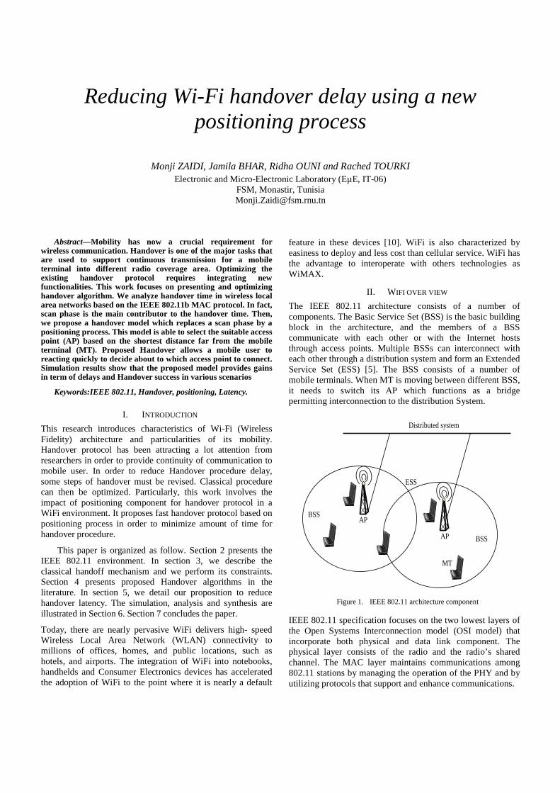
Reducing Wi-Fi handover delay using a new positioning process
Monji ZAIDI, Jamila BHAR, Ridha OUNI and Rached TOURKI Electronic and Micro-Electronic Laboratory (EµE, IT-06)
FSM, Monastir, Tunisia [email protected]
Abstract—Mobility has now a crucial requirement for wireless communication. Handover is one of the major tasks that are used to support continuous transmission for a mobile terminal into different radio coverage area. Optimizing the existing handover protocol requires integrating new functionalities. This work focuses on presenting and optimizing handover algorithm. We analyze handover time in wireless local area networks based on the IEEE 802.11b MAC protocol. In fact, scan phase is the main contributor to the handover time. Then, we propose a handover model which replaces a scan phase by a positioning process. This model is able to select the suitable access point (AP) based on the shortest distance far from the mobile terminal (MT). Proposed Handover allows a mobile user to reacting quickly to decide about to which access point to connect. Simulation results show that the proposed model provides gains in term of delays and Handover success in various scenarios
Keywords:IEEE 802.11, Handover, positioning, Latency.
I. INTRODUCTION
This research introduces characteristics of Wi-Fi (Wireless Fidelity) architecture and particularities of its mobility. Handover protocol has been attracting a lot attention from researchers in order to provide continuity of communication to mobile user. In order to reduce Handover procedure delay, some steps of handover must be revised. Classical procedure can then be optimized. Particularly, this work involves the impact of positioning component for handover protocol in a WiFi environment. It proposes fast handover protocol based on positioning process in order to minimize amount of time for handover procedure.
This paper is organized as follow. Section 2 presents the IEEE 802.11 environment. In section 3, we describe the classical handoff mechanism and we perform its constraints. Section 4 presents proposed Handover algorithms in the literature. In section 5, we detail our proposition to reduce handover latency. The simulation, analysis and synthesis are illustrated in Section 6. Section 7 concludes the paper.
Today, there are nearly pervasive WiFi delivers high- speed Wireless Local Area Network (WLAN) connectivity to millions of offices, homes, and public locations, such as hotels, and airports. The integration of WiFi into notebooks, handhelds and Consumer Electronics devices has accelerated the adoption of WiFi to the point where it is nearly a default
feature in these devices [10]. WiFi is also characterized by easiness to deploy and less cost than cellular service. WiFi has the advantage to interoperate with others technologies as WiMAX.
II. WIFI OVER VIEW
The IEEE 802.11 architecture consists of a number of components. The Basic Service Set (BSS) is the basic building block in the architecture, and the members of a BSS communicate with each other or with the Internet hosts through access points. Multiple BSSs can interconnect with each other through a distribution system and form an Extended Service Set (ESS) [5]. The BSS consists of a number of mobile terminals. When MT is moving between different BSS, it needs to switch its AP which functions as a bridge permitting interconnection to the distribution System.
ESS
BSS
BSS
Distributed system
MT
AP
AP
Figure 1. IEEE 802.11 architecture component
IEEE 802.11 specification focuses on the two lowest layers of the Open Systems Interconnection model (OSI model) that incorporate both physical and data link component. The physical layer consists of the radio and the radio’s shared channel. The MAC layer maintains communications among 802.11 stations by managing the operation of the PHY and by utilizing protocols that support and enhance communications.
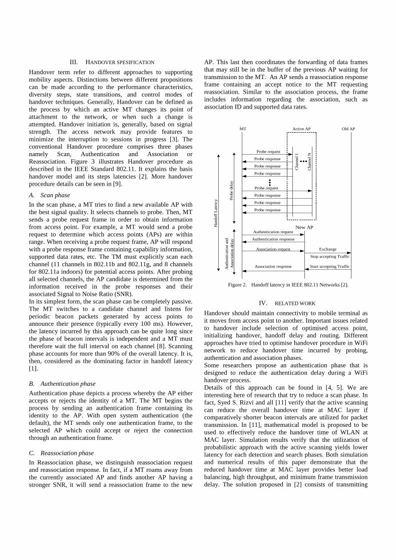
III. HANDOVER SPESIFICATION
Handover term refer to different approaches to supporting mobility aspects. Distinctions between different propositions can be made according to the performance characteristics, diversity steps, state transitions, and control modes of handover techniques. Generally, Handover can be defined as the process by which an active MT changes its point of attachment to the network, or when such a change is attempted. Handover initiation is, generally, based on signal strength. The access network may provide features to minimize the interruption to sessions in progress [3]. The conventional Handover procedure comprises three phases namely Scan, Authentication and Association or Reassociation. Figure 3 illustrates Handover procedure as described in the IEEE Standard 802.11. It explains the basis handover model and its steps latencies [2]. More handover procedure details can be seen in [9].
A. Scan phase
In the scan phase, a MT tries to find a new available AP with the best signal quality. It selects channels to probe. Then, MT sends a probe request frame in order to obtain information from access point. For example, a MT would send a probe request to determine which access points (APs) are within range. When receiving a probe request frame, AP will respond with a probe response frame containing capability information, supported data rates, etc. The TM must explicitly scan each channel (11 channels in 802.11b and 802.11g, and 8 channels for 802.11a indoors) for potential access points. After probing all selected channels, the AP candidate is determined from the information received in the probe responses and their associated Signal to Noise Ratio (SNR). In its simplest form, the scan phase can be completely passive. The MT switches to a candidate channel and listens for periodic beacon packets generated by access points to announce their presence (typically every 100 ms). However, the latency incurred by this approach can be quite long since the phase of beacon intervals is independent and a MT must therefore wait the full interval on each channel [8]. Scanning phase accounts for more than 90% of the overall latency. It is, then, considered as the dominating factor in handoff latency [1].
B. Authentication phase
Authentication phase depicts a process whereby the AP either accepts or rejects the identity of a MT. The MT begins the process by sending an authentication frame containing its identity to the AP. With open system authentication (the default), the MT sends only one authentication frame, to the selected AP which could accept or reject the connection through an authentication frame.
C. Reassociation phase
In Reassociation phase, we distinguish reassociation request and reassociation response. In fact, if a MT roams away from the currently associated AP and finds another AP having a stronger SNR, it will send a reassociation frame to the new
AP. This last then coordinates the forwarding of data frames that may still be in the buffer of the previous AP waiting for transmission to the MT. An AP sends a reassociation response frame containing an accept notice to the MT requesting reassociation. Similar to the association process, the frame includes information regarding the association, such as association ID and supported data rates.
MT Active AP Old AP
New AP
Probe request
Probe response
Probe response
Probe response
Probe request
Probe response
Probe response
Probe response
...
...
Cha
nnel 1
Cha
nnel N
Authentication request
Authentication response
Association request
Association response
Exchange
Stop accepting Traffic
Start accepting Traffic
Hando
ff Late
ncy P
robe
dela
yA
uth
entic
atio
n a
nd
Ass
oci
atio
n de
lay
Figure 2. Handoff latency in IEEE 802.11 Networks [2].
IV. RELATED WORK
Handover should maintain connectivity to mobile terminal as it moves from access point to another. Important issues related to handover include selection of optimised access point, initializing handover, handoff delay and routing. Different approaches have tried to optimise handover procedure in WiFi network to reduce handover time incurred by probing, authentication and association phases. Some researchers propose an authentication phase that is designed to reduce the authentication delay during a WiFi handover process. Details of this approach can be found in [4, 5]. We are interesting here of research that try to reduce a scan phase. In fact, Syed S. Rizvi and all [11] verify that the active scanning can reduce the overall handover time at MAC layer if comparatively shorter beacon intervals are utilized for packet transmission. In [11], mathematical model is proposed to be used to effectively reduce the handover time of WLAN at MAC layer. Simulation results verify that the utilization of probabilistic approach with the active scanning yields lower latency for each detection and search phases. Both simulation and numerical results of this paper demonstrate that the reduced handover time at MAC layer provides better load balancing, high throughput, and minimum frame transmission delay. The solution proposed in [2] consists of transmitting
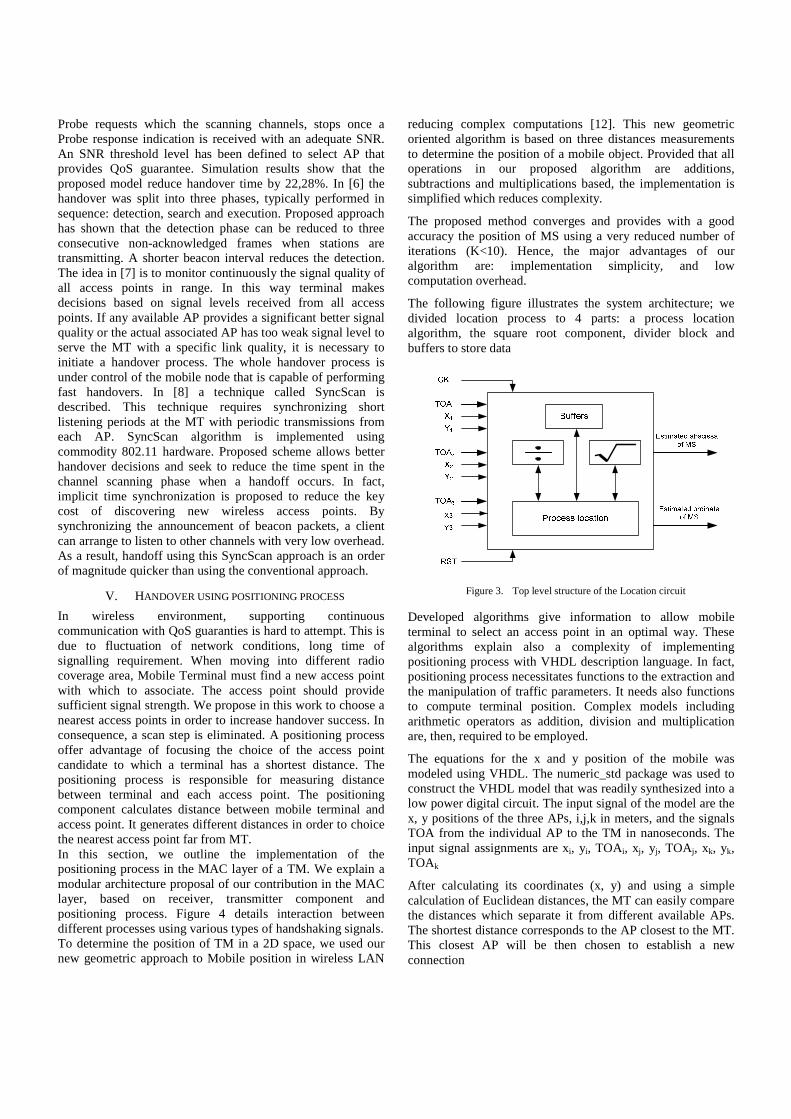
Probe requests which the scanning channels, stops once a Probe response indication is received with an adequate SNR. An SNR threshold level has been defined to select AP that provides QoS guarantee. Simulation results show that the proposed model reduce handover time by 22,28%. In [6] the handover was split into three phases, typically performed in sequence: detection, search and execution. Proposed approach has shown that the detection phase can be reduced to three consecutive non-acknowledged frames when stations are transmitting. A shorter beacon interval reduces the detection. The idea in [7] is to monitor continuously the signal quality of all access points in range. In this way terminal makes decisions based on signal levels received from all access points. If any available AP provides a significant better signal quality or the actual associated AP has too weak signal level to serve the MT with a specific link quality, it is necessary to initiate a handover process. The whole handover process is under control of the mobile node that is capable of performing fast handovers. In [8] a technique called SyncScan is described. This technique requires synchronizing short listening periods at the MT with periodic transmissions from each AP. SyncScan algorithm is implemented using commodity 802.11 hardware. Proposed scheme allows better handover decisions and seek to reduce the time spent in the channel scanning phase when a handoff occurs. In fact, implicit time synchronization is proposed to reduce the key cost of discovering new wireless access points. By synchronizing the announcement of beacon packets, a client can arrange to listen to other channels with very low overhead. As a result, handoff using this SyncScan approach is an order of magnitude quicker than using the conventional approach.
V. HANDOVER USING POSITIONING PROCESS
In wireless environment, supporting continuous communication with QoS guaranties is hard to attempt. This is due to fluctuation of network conditions, long time of signalling requirement. When moving into different radio coverage area, Mobile Terminal must find a new access point with which to associate. The access point should provide sufficient signal strength. We propose in this work to choose a nearest access points in order to increase handover success. In consequence, a scan step is eliminated. A positioning process offer advantage of focusing the choice of the access point candidate to which a terminal has a shortest distance. The positioning process is responsible for measuring distance between terminal and each access point. The positioning component calculates distance between mobile terminal and access point. It generates different distances in order to choice the nearest access point far from MT. In this section, we outline the implementation of the positioning process in the MAC layer of a TM. We explain a modular architecture proposal of our contribution in the MAC layer, based on receiver, transmitter component and positioning process. Figure 4 details interaction between different processes using various types of handshaking signals. To determine the position of TM in a 2D space, we used our new geometric approach to Mobile position in wireless LAN
reducing complex computations [12]. This new geometric oriented algorithm is based on three distances measurements to determine the position of a mobile object. Provided that all operations in our proposed algorithm are additions, subtractions and multiplications based, the implementation is simplified which reduces complexity.
The proposed method converges and provides with a good accuracy the position of MS using a very reduced number of iterations (K<10). Hence, the major advantages of our algorithm are: implementation simplicity, and low computation overhead.
The following figure illustrates the system architecture; we divided location process to 4 parts: a process location algorithm, the square root component, divider block and buffers to store data
Figure 3. Top level structure of the Location circuit
Developed algorithms give information to allow mobile terminal to select an access point in an optimal way. These algorithms explain also a complexity of implementing positioning process with VHDL description language. In fact, positioning process necessitates functions to the extraction and the manipulation of traffic parameters. It needs also functions to compute terminal position. Complex models including arithmetic operators as addition, division and multiplication are, then, required to be employed.
The equations for the x and y position of the mobile was modeled using VHDL. The numeric_std package was used to construct the VHDL model that was readily synthesized into a low power digital circuit. The input signal of the model are the x, y positions of the three APs, i,j,k in meters, and the signals TOA from the individual AP to the TM in nanoseconds. The input signal assignments are xi, yi, TOAi, xj, yj, TOAj, xk, yk, TOAk
After calculating its coordinates (x, y) and using a simple calculation of Euclidean distances, the MT can easily compare the distances which separate it from different available APs. The shortest distance corresponds to the AP closest to the MT. This closest AP will be then chosen to establish a new connection
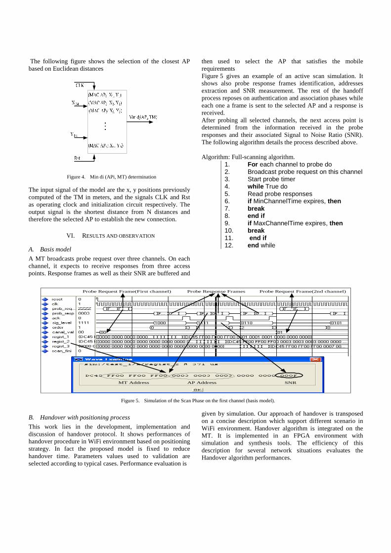
The following figure shows the selection of the closest AP based on Euclidean distances
Figure 4. Min di (APi, MT) determination
The input signal of the model are the x, y positions previously computed of the TM in meters, and the signals CLK and Rst as operating clock and initialization circuit respectively. The output signal is the shortest distance from N distances and therefore the selected AP to establish the new connection.
VI. RESULTS AND OBSERVATION
A. Basis model
A MT broadcasts probe request over three channels. On each channel, it expects to receive responses from three access points. Response frames as well as their SNR are buffered and
then used to select the AP that satisfies the mobile requirements Figure 5 gives an example of an active scan simulation. It shows also probe response frames identification, addresses extraction and SNR measurement. The rest of the handoff process reposes on authentication and association phases while each one a frame is sent to the selected AP and a response is received. After probing all selected channels, the next access point is determined from the information received in the probe responses and their associated Signal to Noise Ratio (SNR). The following algorithm details the process described above. Algorithm: Full-scanning algorithm.
1. For each channel to probe do 2. Broadcast probe request on this channel 3. Start probe timer 4. while True do 5. Read probe responses 6. if MinChannelTime expires, then 7. break 8. end if 9. if MaxChannelTime expires, then 10. break 11. end if 12. end while
Probe Response FramesProbe Request Frame(First channel)
MT Address AP Address SNR
Probe Request Frame(2nd channel)
Figure 5. Simulation of the Scan Phase on the first channel (basis model).
B. Handover with positioning process
This work lies in the development, implementation and discussion of handover protocol. It shows performances of handover procedure in WiFi environment based on positioning strategy. In fact the proposed model is fixed to reduce handover time. Parameters values used to validation are selected according to typical cases. Performance evaluation is
given by simulation. Our approach of handover is transposed on a concise description which support different scenario in WiFi environment. Handover algorithm is integrated on the MT. It is implemented in an FPGA environment with simulation and synthesis tools. The efficiency of this description for several network situations evaluates the Handover algorithm performances.
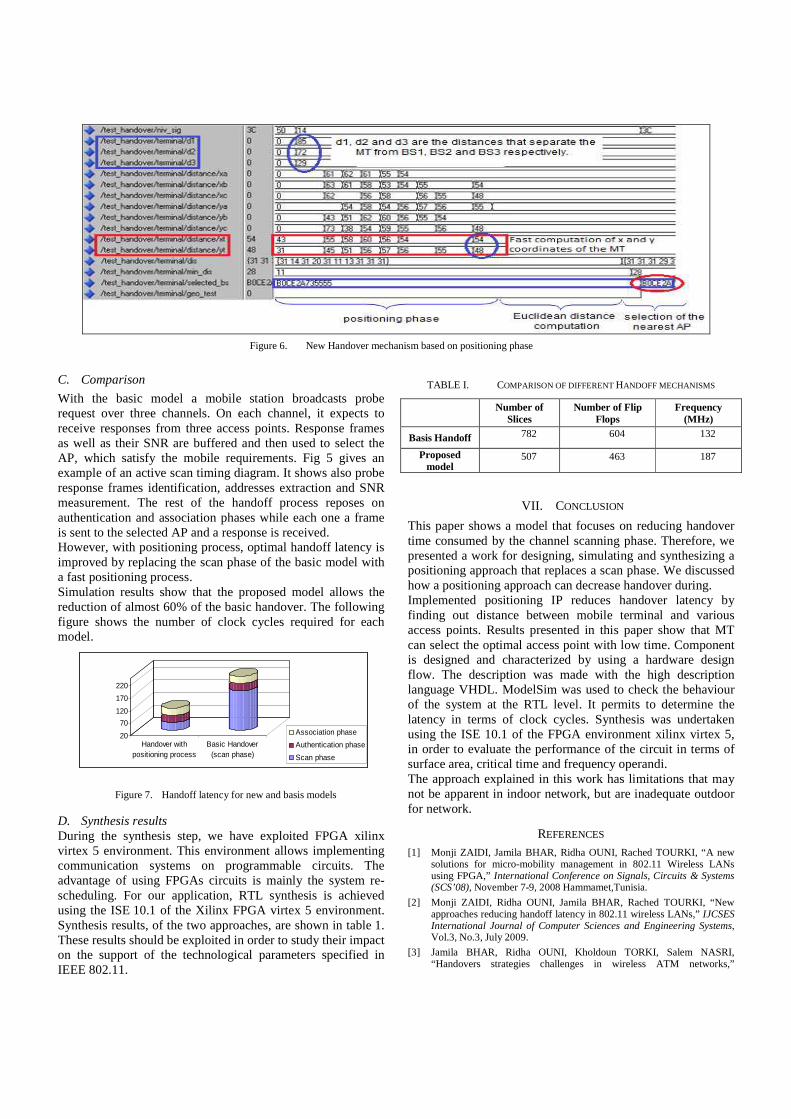
Figure 6. New Handover mechanism based on positioning phase
C. Comparison
With the basic model a mobile station broadcasts probe request over three channels. On each channel, it expects to receive responses from three access points. Response frames as well as their SNR are buffered and then used to select the AP, which satisfy the mobile requirements. Fig 5 gives an example of an active scan timing diagram. It shows also probe response frames identification, addresses extraction and SNR measurement. The rest of the handoff process reposes on authentication and association phases while each one a frame is sent to the selected AP and a response is received. However, with positioning process, optimal handoff latency is improved by replacing the scan phase of the basic model with a fast positioning process. Simulation results show that the proposed model allows the reduction of almost 60% of the basic handover. The following figure shows the number of clock cycles required for each model.
20
70
120
170
220
Handover withpositioning process
Basic Handover(scan phase)
Association phase
Authentication phase
Scan phase
Figure 7. Handoff latency for new and basis models
D. Synthesis results During the synthesis step, we have exploited FPGA xilinx virtex 5 environment. This environment allows implementing communication systems on programmable circuits. The advantage of using FPGAs circuits is mainly the system re-scheduling. For our application, RTL synthesis is achieved using the ISE 10.1 of the Xilinx FPGA virtex 5 environment. Synthesis results, of the two approaches, are shown in table 1. These results should be exploited in order to study their impact on the support of the technological parameters specified in IEEE 802.11.
TABLE I. COMPARISON OF DIFFERENT HANDOFF MECHANISMS
Number of Slices
Number of Flip Flops
Frequency (MHz)
Basis Handoff 782 604 132
Proposed model
507 463 187
VII. CONCLUSION
This paper shows a model that focuses on reducing handover time consumed by the channel scanning phase. Therefore, we presented a work for designing, simulating and synthesizing a positioning approach that replaces a scan phase. We discussed how a positioning approach can decrease handover during. Implemented positioning IP reduces handover latency by finding out distance between mobile terminal and various access points. Results presented in this paper show that MT can select the optimal access point with low time. Component is designed and characterized by using a hardware design flow. The description was made with the high description language VHDL. ModelSim was used to check the behaviour of the system at the RTL level. It permits to determine the latency in terms of clock cycles. Synthesis was undertaken using the ISE 10.1 of the FPGA environment xilinx virtex 5, in order to evaluate the performance of the circuit in terms of surface area, critical time and frequency operandi. The approach explained in this work has limitations that may not be apparent in indoor network, but are inadequate outdoor for network.
REFERENCES [1] Monji ZAIDI, Jamila BHAR, Ridha OUNI, Rached TOURKI, “A new
solutions for micro-mobility management in 802.11 Wireless LANs using FPGA,” International Conference on Signals, Circuits & Systems (SCS’08), November 7-9, 2008 Hammamet,Tunisia.
[2] Monji ZAIDI, Ridha OUNI, Jamila BHAR, Rached TOURKI, “New approaches reducing handoff latency in 802.11 wireless LANs,” IJCSES International Journal of Computer Sciences and Engineering Systems, Vol.3, No.3, July 2009.
[3] Jamila BHAR, Ridha OUNI, Kholdoun TORKI, Salem NASRI, “Handovers strategies challenges in wireless ATM networks,”
International Journal of Applied Mathematics and Computer Sciences, 4 (2): April 2007, pp 636-641.
[4] András Bohák, Levente Buttyán, and László Dóra “An authentication scheme for fast handover between WiFi access points,” WICON 2007, October 22-24, 2007.
[5] Jidong,Wang and Lichun Bao, “Mobile Context Handoff in Distributed IEEE 802.11 Systems, ”Bren School of Information and Computer Sciences, University of California,Irvine, CA 92697.
[6] Héctor Velayos, Gunnar Karlsson, “Techniques to Reduce IEEE 802.11b MAC Layer Handover Time,” TRITA-IMIT-LCN R 03:02 ISSN 1651-7717,ISRN KTH/IMIT/LCN/R-03/02--SE. April 2003.
[7] Norbert Jordan, Reinhard Fleck, Christian Ploninger “Fast Handover
Support in Wireless LAN based Networks, ” Institute of Communication Networks, Vienna University of Technology Favoritenstrasse 9/388, A-1040 Vienna, Austria
[8] I. Ramani and S. Savage, “SyncScan: Practical Fast Handoff for 802.11 Infrastructure Networks,” Proceedings of the IEEE Infocom, March 2005.
[9] Arunesh Mishra, Minho Shin, William Arbaugh. “An Empirical Analysis of the IEEE 802.11 MAC Layer Handoff Process,” CS Tech Report NumberCS-TR-4395. UMIACS Tech Report Number UMIACSTR-2002-75
[10] A. Saeed, Hafizal Mohamad, Borhanuddin Mohd. Ali & Mazlan Abbas, “Vertical Handover Algorithm for WiMAX/WiFi Interworking,” International Journal of Engineering (IJE), Volume (3) : Issue (5).2008.
[11] Syed S. Rizvi, Aasia Riasat, and Khaled M, A Elleithy “QUANTITATIVE ANALYSIS OF HANDOVER TIME AT MAC LAYER FOR WIRELESS MOBILE NETWORKS, ” International Journal of Wireless & Mobile Networks (IJWMN), Vol 1, No 2, November 2009
[12] Monji ZAIDI, Rached TOURKI, Ridha OUNI “A New geometric Approach to Mobile Position in wireless LAN reducing complex computations,” 2010 International Conference on Design & Technology of Integrated Systems in Nanoscale Era(DTIS 2010) , Hammamet Tunisia March 23-25 2010.
WORLDCOMP'11-ICOMP'11- ICW2941
Novel Data Harvesting Scheme for Efficient Data Aggregation
Mohammad Zuheir Hourani, Ridha OUNI College of Computer and Information Sciences
Computer Engineering Department P.O.Box 51178, Riyadh 11543, KSA
Abstract—The basic idea behind intelligent transportation system is how to deploy vehicular sensor network that have many characteristic such as high computation power ,enough storage space and mobile sensor node in order to design an effective and efficient architecture for data collection and data exchange. In this paper we will introduce an intelligent transportation system with new network paradigm to collect important information from the road environment based on the vehicular sensor network (VSN). Data aggregate provides the drivers by valuable information in order to make the road safer and less congested. Our system framework consists of active vehicular sensor node, passive vehicular sensor node and sink node distributed according to the road segmentation for collecting data from active vehicular sensor node passing by, while active vehicular sensor node collect data from passive vehicular sensor node in their segment using multihop data harvesting. Our scheme aims to reduce broadcast storm and avoid collision. Finally, the simulation using the OPNET simulator shows the effectiveness of the proposed schema.
Keyword- ITS, VSN, IVS, data harvesting, hybrid architecture, data aggregation.
I. INTRODUCTION
Significant advances in manufacturing technology equipment and the advent of Micro-Electro-Mechanical Switches (MEMS) has opened the way for the construction of intelligent sensor nodes which are able to perform three major functions: sensing, processing and wireless communication. These wireless sensor nodes are characterized by their intelligence, their small size, low cost, battery powered, and easy to install and repair. These features open doors to deploy WSNs in the future for a wide range of applications because it greatly expands our ability to monitor and control the physical environment from remote locations.
An interesting field where the use of WSNs proves effectiveness is the field of Intelligent Vehicular Systems. An Intelligent Vehicular System (IVS) uses technological
advances in computers and information technology to improve the efficiency of both new and existing vehicular systems.
Vehicular sensor networks (VSNs) is a technology where sensors are deployed in the road side and in the vehicles to sense various urban phenomenon’s and transmit information for vehicular traffic control and monitoring. VSNs have different characteristic from traditional sensor network (static network), interns of mobility, computational, power supply, memory storage and reliability. Moreover vehicular sensor network VSN has a much more dynamic topology as compared to the static WSN. It is often assumed that VSN will move continuously in a random fashion, thus making the whole network a very dynamic topology. This dynamic nature of VSN is reflected in the choice of other characteristic properties, such as routing, MAC level protocols and physical hardware, beside this, dynamic topology of vehicular sensor network VSN, communication links can often become unreliable [1]. The previous characteristics allow deploying vehicular wireless sensor network to design intelligent transportation system.
In this paper we are interested to design an optimal system architecture for such vehicular sensor network for vehicular traffic control and monitoring. several assumption have been made. First, we assume that vehicles communicate through a wireless interface, implementing a CSMA/CA MAC layer protocol that provides a RTS/CTS/DATA/ACK handshake sequence for each transmission. Vehicular sensor network adopt IEEE 802.11 as a cost efficient and widely deployed solution for network communication. IEEE 802.11p is a draft amendment to IEEE 802.11 standard to add wireless access in vehicular environment. It supports data exchange for vehicle to vehicle (V2V) and vehicle to infrastructure (V2I) in the licensed ITS band of 5.9 GHz.
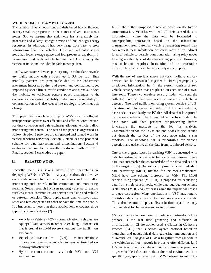
WORLDCOMP'11-ICOMP'11- ICW2941 The number of sink nodes that are distributed beside the road is very small in proportion to the number of vehicular sensor nodes. So, we assume that sink node has a relatively fast processor and a large storage device and has enough energy resources. In addition, it has very large data base to store information from the vehicles. However, vehicular sensor node has lower storage space and low processor capability. It is assumed that each vehicle has unique ID to identify the vehicular node and included in each message sent.
Finally, we assume devices participating in vehicular networks are highly mobile with a speed up to 30 m/s. But, their mobility patterns are predictable due to the constrained movement imposed by the road system and constrained speed imposed by speed limits, traffic conditions and signals. In fact, the mobility of vehicular sensors poses challenges to the communication system. Mobility undermines the reliability of communication and also causes the topology to continuously change.
This paper focus on how to deploy WSN as an intelligent transportation system over effective and efficient architecture for data collection and data exchange allowing vehicle traffic monitoring and control. The rest of the paper is organized as follow. Section 2 provides a back ground and related work in vehicular sensor networks. Section 3 introduces the proposed scheme for data harvesting and dissemination. Section 4 evaluates the simulation results conducted with OPNET. Finally, section 5 concludes the paper.
II. RELATED WORK
Recently, there is a strong interest from researcher’s in deploying WSNs in VSNs in many applications that involve constraints related to the traffic conditions such as traffic monitoring and control, traffic estimation and monitoring parking. Some research focus in moving vehicles to enable wireless sensor communication between roadside and vehicle or between vehicles. These applications aim to make roads safer and less congested in order to save the time for people. It’s important to note that these applications encounter three types of communications [2]:
• Vehicle-to-Vehicle (V2V) communication: vehicles are equipped with sensors in order to exchange information that is crucial to avoid severe situations like traffic jam avoidance.
• Vehicle-to-Infrastructure (V2I) communications: information flow from vehicles to sensors installed on roadway infrastructure
• Hybrid communication: uses both V2V and V2I architecture
In [3] the author proposed a scheme based on the hybrid communication. Vehicles will send all their sensed data to infostations, where the data will be forwarded to corresponding infostation based on the infostations management area. Later, any vehicle requesting sensed data can request these infostation, which is more of an indirect form of vehicle to vehicle communication using relay nodes forming another type of data harvesting protocol. However, this technique requires installation of an infostation infrastructure, which can be very costly and complex.
With the use of wireless sensor network, multiple sensory devices can be networked together to share geographically distributed information. In [4], the system consists of two vehicle sensory nodes that are placed on each side of a two-lane road. These two wireless sensory nodes will send the collected data to the base node whenever a vehicle is detected. The road traffic monitoring system consists of a 3-tier structure. The system is made up of the end-node tier, base node tier and lastly the PC tier. All data that is captured by the end-nodes will be forwarded to the base node. The base node will then perform pre-processing before forwarding the message to the PC for analysis. Communication via the PC to the end nodes is also carried out through the services of the base node using a star topology. The end-node tier is responsible for vehicle detection and gathering all the data from its onboard sensors.
One of the biggest issues in realizing VSN is concerned with data harvesting which is a technique where sensors create data that summarize the characteristic of the data and send it to the target. In [5], the author proposed a novel multi-hop data harvesting (MDH) method for the V2I architecture. MDH have two scheme proposed for VSN. The MDH scheme using replicas (MDH-R) is proposed for requesting data from single sensor node, while data aggregation scheme is designed (MDH-RA) for cases when the request was made to a geo cast region. Many applications in VSN may require multi-hop data transmission to meet real-time constraints. The author see multi-hop data dissemination capabilities may become ideal for future researches in this area.
VSNs come out as new brand of vehicular networks, whose propose is the real time gathering and diffusion of information. In [2] the author used a Clustering Gathering Protocol (CGP) that is across layered protocol based on hierarchal and geographical data gathering, aggregation and dissemination. The goal of CGP is to gather from all node in the vehicular ad hoc network in order to offer different kind ITS services, it allows telecommunication/service providers to get valuable information about the road environment in a specific geographical area, using V2V network to minimize
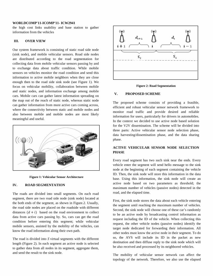
WORLDCOMP'11-ICOMP'11- ICW2941 the high cost links usability and base station to gather information from the vehicles
III. OVER VIEW
Our system framework is consisting of static road side node (sink node), and mobile vehicular sensors. Road side nodes are distributed according to the road segmentation for collecting data from mobile vehicular sensors passing by and to exchange data about traffic condition. While mobile sensors on vehicles monitor the road condition and send this information to active mobile neighbors when they are close enough then to the road side sink node (see Figure 1). We focus on vehicular mobility, collaboration between mobile and static nodes, and information exchange among mobile cars. Mobile cars can gather latest information spreading on the map out of the reach of static node, whereas static node can gather information from more active cars coming across, where the connectivity between static and mobile nodes and also between mobile and mobile nodes are most likely meaningful and useful.
Figure 1: Vehicular Sensor Architecture
IV. ROAD SEGMENTATION
The roads are divided into small segments. On each road segment, there are two road side node (sink node) located at the both ends of the segment, as shown in Figure.2. Usually, the road side nodes are placed on the roadside with different distances (𝑑𝑑 + 𝑖𝑖) based on the road environment to collect data from active cars passing by. So, cars can get the road condition before entering this segment; while vehicular mobile sensors, assisted by the mobility of the vehicles, can know the road information along their own path.
The road is divided into 𝑆𝑆 virtual segments with the different length (Figure 2). In each segment an active node is selected to gather data from all nodes in its segment, aggregate them, and send the result to the sink node.
Figure 2: Road Segmentation
V. PROPOSED SCHEME
The proposed scheme consists of providing a feasible, efficient and robust vehicular sensor network framework to monitor road traffic and provide desired and reliable information for users, particularly for drivers in automobiles. In the context we decided to use active node based solution for the V2V dissemination. The scheme will be divided into three parts: Active vehicular sensor node selection phase, data harvesting/dissemination phase, and the data sharing phase.
ACTIVE VEHICULAR SENSOR NODE SELECTION PHASE
Every road segment has two such sink near the ends. Every vehicle enter the segment will send hello message to the sink node at the beginning of each segment containing the vehicle ID. Then, the sink node will store this information in the data base. Using this information, the sink node will create an active node based on two parameters as threshold; the maximum number of vehicles (passive nodes) detected in the road, and the elapsed time.
First, the sink node stores the data about each vehicle entering the segment until reaching the maximum number of vehicles. Second, the sink node will choose one of these car’s randomly to be an active node by broadcasting control information as request including the ID of the vehicle. When collecting this request, the other vehicle nodes (passive nodes) identify the target node dedicated for forwarding their information. All other nodes must know the active node in their segment. To do so, the AVS will include its ID in the packet as new destination and then diffuse reply to the sink node which will be also received and processed by its neighbored vehicles.
The mobility of vehicular sensor network can affect the topology of the network. Therefore, we also use the elapsed
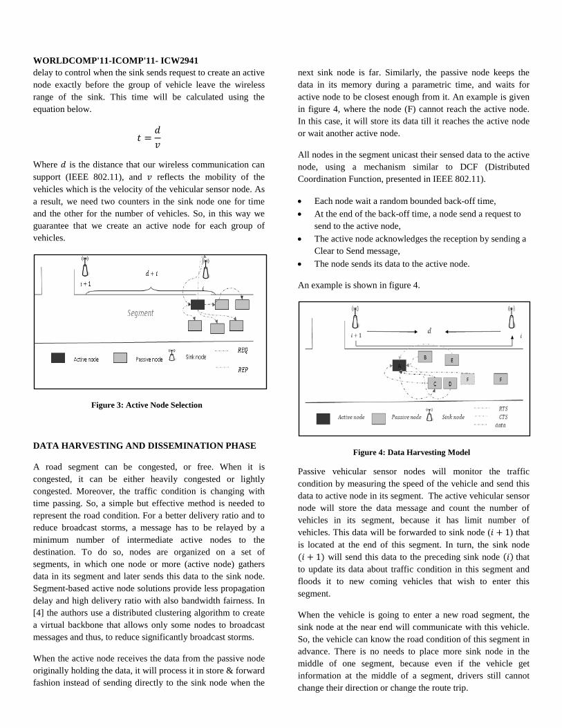
WORLDCOMP'11-ICOMP'11- ICW2941 delay to control when the sink sends request to create an active node exactly before the group of vehicle leave the wireless range of the sink. This time will be calculated using the equation below.
𝑡𝑡 =𝑑𝑑𝑣𝑣
Where 𝑑𝑑 is the distance that our wireless communication can support (IEEE 802.11), and 𝑣𝑣 reflects the mobility of the vehicles which is the velocity of the vehicular sensor node. As a result, we need two counters in the sink node one for time and the other for the number of vehicles. So, in this way we guarantee that we create an active node for each group of vehicles.
Figure 3: Active Node Selection
DATA HARVESTING AND DISSEMINATION PHASE
A road segment can be congested, or free. When it is congested, it can be either heavily congested or lightly congested. Moreover, the traffic condition is changing with time passing. So, a simple but effective method is needed to represent the road condition. For a better delivery ratio and to reduce broadcast storms, a message has to be relayed by a minimum number of intermediate active nodes to the destination. To do so, nodes are organized on a set of segments, in which one node or more (active node) gathers data in its segment and later sends this data to the sink node. Segment-based active node solutions provide less propagation delay and high delivery ratio with also bandwidth fairness. In [4] the authors use a distributed clustering algorithm to create a virtual backbone that allows only some nodes to broadcast messages and thus, to reduce significantly broadcast storms.
When the active node receives the data from the passive node originally holding the data, it will process it in store & forward fashion instead of sending directly to the sink node when the
next sink node is far. Similarly, the passive node keeps the data in its memory during a parametric time, and waits for active node to be closest enough from it. An example is given in figure 4, where the node (F) cannot reach the active node. In this case, it will store its data till it reaches the active node or wait another active node.
All nodes in the segment unicast their sensed data to the active node, using a mechanism similar to DCF (Distributed Coordination Function, presented in IEEE 802.11).
• Each node wait a random bounded back-off time, • At the end of the back-off time, a node send a request to
send to the active node, • The active node acknowledges the reception by sending a
Clear to Send message, • The node sends its data to the active node.
An example is shown in figure 4.
Figure 4: Data Harvesting Model
Passive vehicular sensor nodes will monitor the traffic condition by measuring the speed of the vehicle and send this data to active node in its segment. The active vehicular sensor node will store the data message and count the number of vehicles in its segment, because it has limit number of vehicles. This data will be forwarded to sink node (𝑖𝑖 + 1) that is located at the end of this segment. In turn, the sink node (𝑖𝑖 + 1) will send this data to the preceding sink node (𝑖𝑖) that to update its data about traffic condition in this segment and floods it to new coming vehicles that wish to enter this segment.
When the vehicle is going to enter a new road segment, the sink node at the near end will communicate with this vehicle. So, the vehicle can know the road condition of this segment in advance. There is no needs to place more sink node in the middle of one segment, because even if the vehicle get information at the middle of a segment, drivers still cannot change their direction or change the route trip.
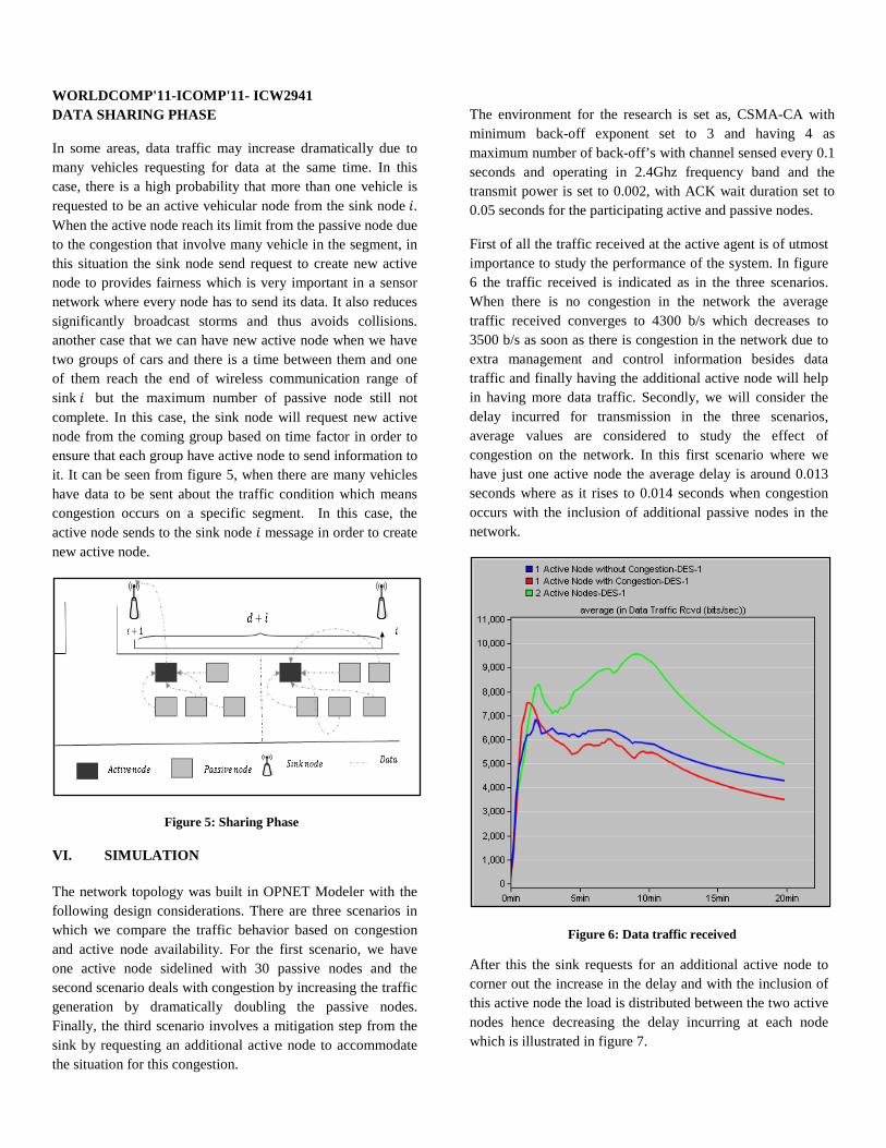
WORLDCOMP'11-ICOMP'11- ICW2941 DATA SHARING PHASE
In some areas, data traffic may increase dramatically due to many vehicles requesting for data at the same time. In this case, there is a high probability that more than one vehicle is requested to be an active vehicular node from the sink node 𝑖𝑖. When the active node reach its limit from the passive node due to the congestion that involve many vehicle in the segment, in this situation the sink node send request to create new active node to provides fairness which is very important in a sensor network where every node has to send its data. It also reduces significantly broadcast storms and thus avoids collisions. another case that we can have new active node when we have two groups of cars and there is a time between them and one of them reach the end of wireless communication range of sink 𝑖𝑖 but the maximum number of passive node still not complete. In this case, the sink node will request new active node from the coming group based on time factor in order to ensure that each group have active node to send information to it. It can be seen from figure 5, when there are many vehicles have data to be sent about the traffic condition which means congestion occurs on a specific segment. In this case, the active node sends to the sink node 𝑖𝑖 message in order to create new active node.
Figure 5: Sharing Phase
VI. SIMULATION
The network topology was built in OPNET Modeler with the following design considerations. There are three scenarios in which we compare the traffic behavior based on congestion and active node availability. For the first scenario, we have one active node sidelined with 30 passive nodes and the second scenario deals with congestion by increasing the traffic generation by dramatically doubling the passive nodes. Finally, the third scenario involves a mitigation step from the sink by requesting an additional active node to accommodate the situation for this congestion.
The environment for the research is set as, CSMA-CA with minimum back-off exponent set to 3 and having 4 as maximum number of back-off’s with channel sensed every 0.1 seconds and operating in 2.4Ghz frequency band and the transmit power is set to 0.002, with ACK wait duration set to 0.05 seconds for the participating active and passive nodes.
First of all the traffic received at the active agent is of utmost importance to study the performance of the system. In figure 6 the traffic received is indicated as in the three scenarios. When there is no congestion in the network the average traffic received converges to 4300 b/s which decreases to 3500 b/s as soon as there is congestion in the network due to extra management and control information besides data traffic and finally having the additional active node will help in having more data traffic. Secondly, we will consider the delay incurred for transmission in the three scenarios, average values are considered to study the effect of congestion on the network. In this first scenario where we have just one active node the average delay is around 0.013 seconds where as it rises to 0.014 seconds when congestion occurs with the inclusion of additional passive nodes in the network.
Figure 6: Data traffic received
After this the sink requests for an additional active node to corner out the increase in the delay and with the inclusion of this active node the load is distributed between the two active nodes hence decreasing the delay incurring at each node which is illustrated in figure 7.
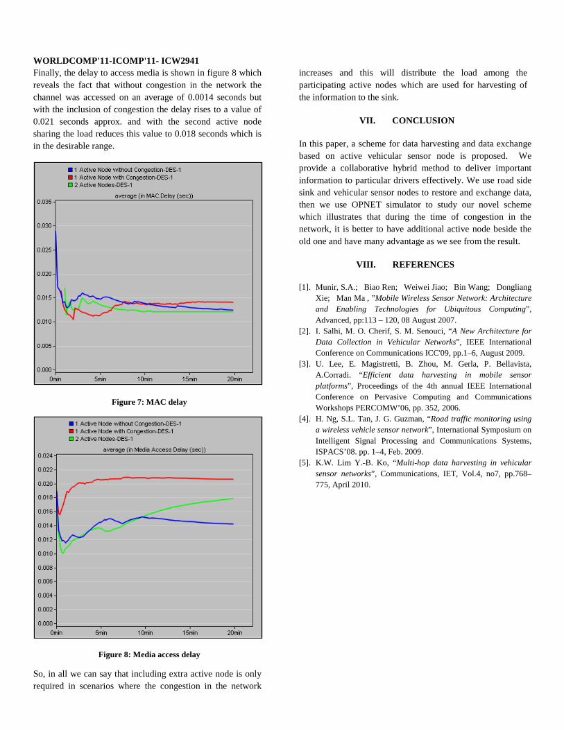
WORLDCOMP'11-ICOMP'11- ICW2941 Finally, the delay to access media is shown in figure 8 which reveals the fact that without congestion in the network the channel was accessed on an average of 0.0014 seconds but with the inclusion of congestion the delay rises to a value of 0.021 seconds approx. and with the second active node sharing the load reduces this value to 0.018 seconds which is in the desirable range.
Figure 7: MAC delay
Figure 8: Media access delay
So, in all we can say that including extra active node is only required in scenarios where the congestion in the network
increases and this will distribute the load among the participating active nodes which are used for harvesting of the information to the sink.
VII. CONCLUSION
In this paper, a scheme for data harvesting and data exchange based on active vehicular sensor node is proposed. We provide a collaborative hybrid method to deliver important information to particular drivers effectively. We use road side sink and vehicular sensor nodes to restore and exchange data, then we use OPNET simulator to study our novel scheme which illustrates that during the time of congestion in the network, it is better to have additional active node beside the old one and have many advantage as we see from the result.
VIII. REFERENCES
[1]. Munir, S.A.; Biao Ren; Weiwei Jiao; Bin Wang; Dongliang Xie; Man Ma , ”Mobile Wireless Sensor Network: Architecture and Enabling Technologies for Ubiquitous Computing”, Advanced, pp:113 – 120, 08 August 2007.
[2]. I. Salhi, M. O. Cherif, S. M. Senouci, “A New Architecture for Data Collection in Vehicular Networks”, IEEE International Conference on Communications ICC'09, pp.1–6, August 2009.
[3]. U. Lee, E. Magistretti, B. Zhou, M. Gerla, P. Bellavista, A.Corradi. “Efficient data harvesting in mobile sensor platforms”, Proceedings of the 4th annual IEEE International Conference on Pervasive Computing and Communications Workshops PERCOMW’06, pp. 352, 2006.
[4]. H. Ng, S.L. Tan, J. G. Guzman, “Road traffic monitoring using a wireless vehicle sensor network”, International Symposium on Intelligent Signal Processing and Communications Systems, ISPACS’08. pp. 1–4, Feb. 2009.
[5]. K.W. Lim Y.-B. Ko, “Multi-hop data harvesting in vehicular sensor networks”, Communications, IET, Vol.4, no7, pp.768–775, April 2010.
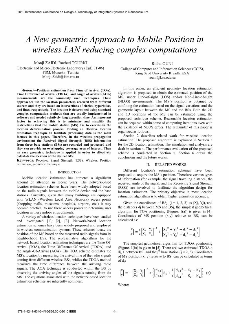
A New geometric Approach to Mobile Position in wireless LAN reducing complex computations
Monji ZAIDI, Rached TOURKI Electronic and Micro-Electronic Laboratory (EµE, IT-06)
FSM, Monastir, Tunisia [email protected]
Ridha OUNI College of Computer and Information Sciences (CCIS),
King Saud University Riyadh, KSA [email protected]
Abstract—Positions estimation from Time of Arrival (TOA), Time Difference of Arrival (TDOA), and Angle of Arrival (AOA) measurements are the commonly used techniques. These approaches use the location parameters received from different sources and they are based on intersections of circles, hyperbolas, and lines, respectively. The location is determined using standard complex computation methods that are usually implemented in software and needed relatively long execution time. An important factor in achieving this is to minimize and simplify the instructions that the mobile station (MS) has to execute in the location determination process. Finding an effective location estimation technique to facilitate processing data is the main focuses in this paper. Therefore, in the wireless propagation environment the Received Signal Strength (RSS) information from three base stations (BSs) are recorded and processed and they can provide an overlapping coverage area of interest. Then an easy geometric technique is applied in order to effectively calculate the location of the desired MS. Keywords: Received Signal Strength (RSS), Wireless, Position estimation, geometric technique
I. INTRODUCTION
Mobile location estimation has attracted a significant amount of attention in recent years. The network-based location estimation schemes have been widely adopted based on the radio signals between the mobile device and the base stations. Currently, given that many buildings are equipped with WLAN (Wireless Local Area Network) access points (shopping malls, museums, hospitals, airports, etc.) it may become practical to use these access points to determine user location in these indoor environments.
A variety of wireless location techniques have been studied and investigated [1], [2], [3]. Network-based location estimation schemes have been widely proposed and employed in wireless communication systems. These schemes locate the position of the MS based on the measured radio signals from its neighborhood BSs. The representative algorithms for the network-based location estimation techniques are the Time-Of-Arrival (TOA), the Time Difference-Of-Arrival (TDOA), and the Angle-Of-Arrival (AOA). The TOA scheme estimates the MS’s location by measuring the arrival time of the radio signals coming from different wireless BSs, whiles the TDOA method measures the time difference between the arriving radio signals. The AOA technique is conducted within the BS by observing the arriving angles of the signals coming from the MS. The equations associated with the network-based location estimation schemes are inherently nonlinear.
In this paper, an efficient geometry location estimation algorithm is proposed to obtain the estimated position of the MS, under Line-of-sight (LOS) and/or Non-Line-of-sight (NLOS) environments. The MS’s position is obtained by confining the estimation based on the signal variations and the geometric layout between the MS and the BSs. Both the 2D and 3D locations of the MS can be estimated using the proposed technique scheme. Reasonable location estimation can be acquired within some of computing iterations even with the existence of NLOS errors. The remainder of this paper is organized as follows:
Section 2 describes related work for wireless location estimation. The proposed algorithm is explained in Section 3 for the 2D location estimation. The simulation and analysis are dealt in section 4. The performance evaluation of the proposed scheme is conducted in Section 5. Section 6 draws the conclusions and the future works.
II. RELATED WORKS Different location’s estimation schemes have been
proposed to acquire the MS’s position. Therefore various types of information (for example, the signal traveling distance, the received angle of the signal, and the Receiving Signal Strength (RSS)) are involved to facilitate the algorithm design for location estimation. The primary objective in most location estimation algorithms is to obtain higher estimation accuracy.
Given the coordinates of BSj, (j = 1, 2, 3) as (Xj, Yj), and the distances dj between MS and BSj, the simplest geometrical algorithm for TOA positioning (Figure. 1(a)) is given in [4]. Coordinates of MS position (x,y) relative to BS1 can be calculated as:
���� � �� ������ ���� �
�� � ��� � ��� � ��� � ��� � � � � � ��� � � �� The simplest geometrical algorithm for TDOA positioning
(Figure. 1(b)) is given in [5]. There are two estimated TDOA-s dj, 1 between BS1 and the jth base station (j = 2, 3). Coordinates of MS position (x, y) relative to BS1 can be calculated in terms of d1:
���� � � ������ ���� ��� � ������ ��� �� �
�� �
����� � �� � ��� ��� � � � ��
�������
Where:
2010 International Conference on Design & Technology of Integrated Systems in Nanoscale Era
-1-978-1-4244-6340-4/10/$26.00 ©2010 IEEE
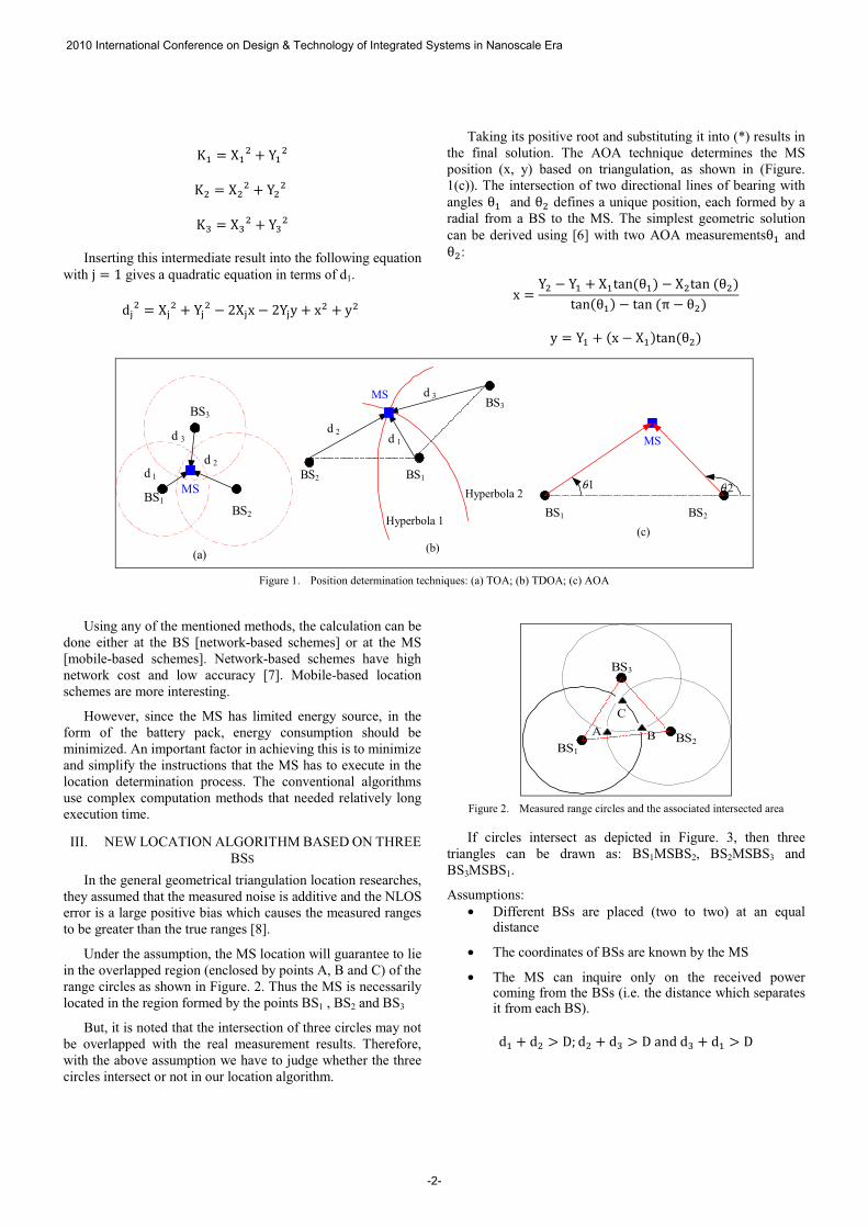
�� � �� � ���
�� � �� � ���
� � � � � ��Inserting this intermediate result into the following equation
with � � � gives a quadratic equation in terms of d1.
��� � �� � ��� � ��� � ���� � �� � ��
Taking its positive root and substituting it into (*) results in the final solution. The AOA technique determines the MS position (x, y) based on triangulation, as shown in (Figure. 1(c)). The intersection of two directional lines of bearing with angles � and � defines a unique position, each formed by a radial from a BS to the MS. The simplest geometric solution can be derived using [6] with two AOA measurements � and �:
� � �� � �� � �!"#� �� � �!"#�� ��!"#� �� � !"#��$ � ��
� � �� � �� � ��!"#� ��
�
BS1BS2
BS3MS
Hyperbola 1
Hyperbola 2
d 1d 2
d 3
(b)
BS1
BS3
BS2
d 1
d 2
d 3
MS
(a)
BS1 BS2
MS
2θ1θ
(c)
��Figure 1. Position determination techniques: (a) TOA; (b) TDOA; (c) AOA
�Using any of the mentioned methods, the calculation can be
done either at the BS [network-based schemes] or at the MS [mobile-based schemes]. Network-based schemes have high network cost and low accuracy [7]. Mobile-based location schemes are more interesting.
However, since the MS has limited energy source, in the form of the battery pack, energy consumption should be minimized. An important factor in achieving this is to minimize and simplify the instructions that the MS has to execute in the location determination process. The conventional algorithms use complex computation methods that needed relatively long execution time.
III. NEW LOCATION ALGORITHM BASED ON THREEBSS
In the general geometrical triangulation location researches, they assumed that the measured noise is additive and the NLOS error is a large positive bias which causes the measured ranges to be greater than the true ranges [8].
Under the assumption, the MS location will guarantee to lie in the overlapped region (enclosed by points A, B and C) of the range circles as shown in Figure. 2. Thus the MS is necessarily located in the region formed by the points BS1 , BS2 and BS3
But, it is noted that the intersection of three circles may not be overlapped with the real measurement results. Therefore, with the above assumption we have to judge whether the three circles intersect or not in our location algorithm.
BS1BS2
BS3
A B
C
�Figure 2. Measured range circles and the associated intersected area
If circles intersect as depicted in Figure. 3, then three triangles can be drawn as: BS1MSBS2, BS2MSBS3 and BS3MSBS1.
Assumptions: • Different BSs are placed (two to two) at an equal
distance
• The coordinates of BSs are known by the MS
• The MS can inquire only on the received power coming from the BSs (i.e. the distance which separates it from each BS).
�� � �� % &' �� � � % &�"#��� � �� % &
2010 International Conference on Design & Technology of Integrated Systems in Nanoscale Era
-2-
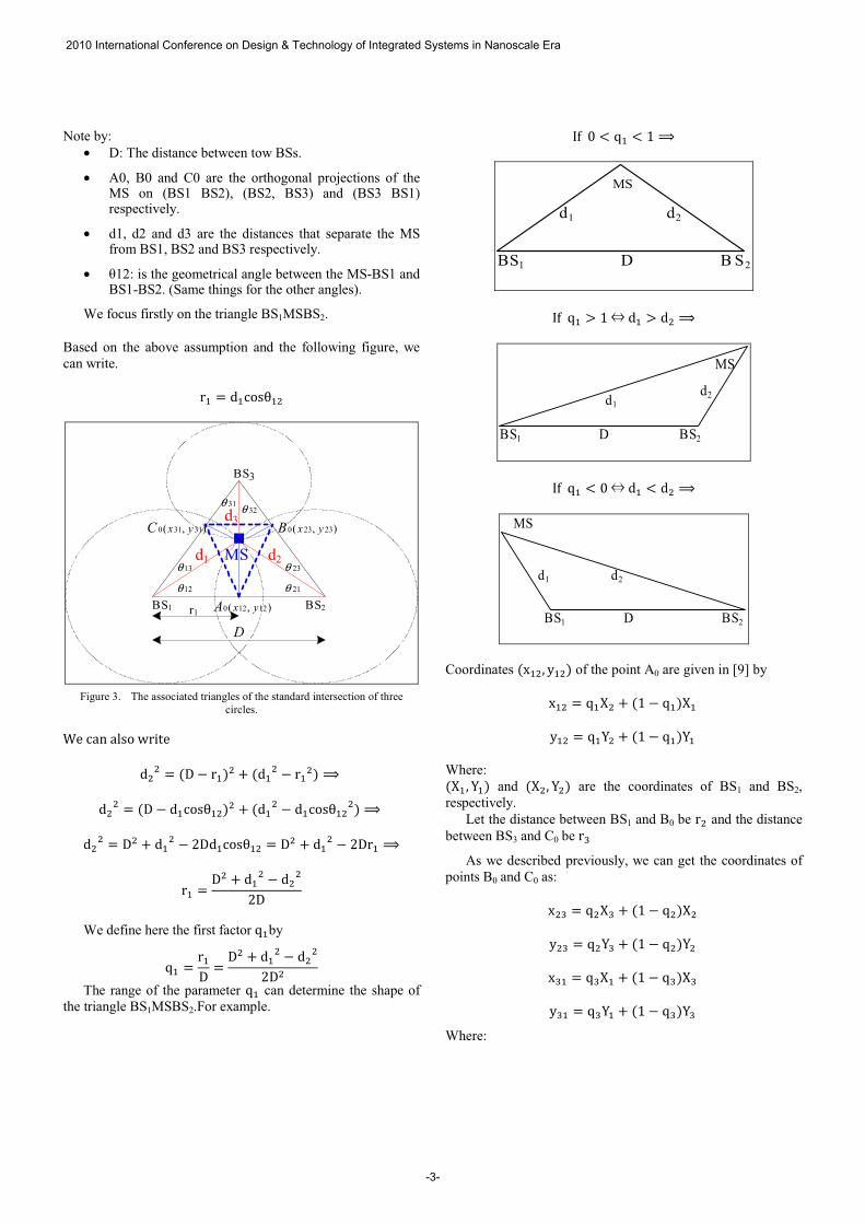
Note by: • D: The distance between tow BSs.
• A0, B0 and C0 are the orthogonal projections of the MS on (BS1 BS2), (BS2, BS3) and (BS3 BS1) respectively.
• d1, d2 and d3 are the distances that separate the MS from BS1, BS2 and BS3 respectively.
• �12: is the geometrical angle between the MS-BS1 and BS1-BS2. (Same things for the other angles).
We focus firstly on the triangle BS1MSBS2.
Based on the above assumption and the following figure, we can write.
(� � ��)*+ ��
BS1 BS2
BS3
MS d1 d2
d3
23θ
21θ12θ
13θ
32θ31θ
),( 12120 yxA
),( 23230 yxB),( 31310 yxC
D r1
Figure 3. The associated triangles of the standard intersection of three circles.
,-�)"#�".+*�/(0!-���� � �& � (��� � ���� � (��� 1
��� � �& � ��)*+ ���� � ���� � ��)*+ ���� 1
��� � &� � ��� � �&��)*+ �� � &� � ��� � �&(� 1
(� � &� � ��� � ����&
We define here the first factor 2�by
2� � (�& � &� � ��� � ����&� �The range of the parameter 2� can determine the shape of
the triangle BS1MSBS2.For example.
��
34��5 6 2� 6 � 1�
B S2
MS
d1 d2
D BS1
34��2� % ������ % �� 1�
D BS2BS1
MS
d1 d2
34��2� 6 5����� 6 �� 1�
BS1 BS2D
d1 d2
MS
Coordinates ����� ���� of the point A0 are given in [9] by
��� � 2�� � �� � 2�������� � 2��� � �� � 2�����
Where: ��� ��� and ��� ��� are the coordinates of BS1 and BS2, respectively.
Let the distance between BS1 and B0 be (� and the distance between BS3 and C0 be (
As we described previously, we can get the coordinates of points B0 and C0 as:
�� � 2� � �� � 2���� �� � 2�� � �� � 2����� � � � 2 � � �� � 2 � � � � � 2 �� � �� � 2 �� �
Where:
2010 International Conference on Design & Technology of Integrated Systems in Nanoscale Era
-3-
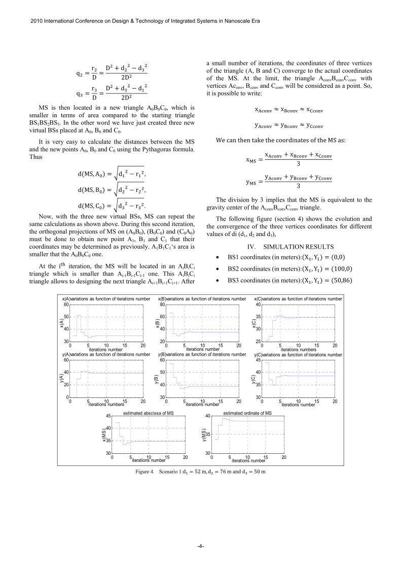
2� � (�& � &� � ��� � � ��&�
2 � ( & � &� � � � � ����&�
MS is then located in a new triangle A0B0C0, which is smaller in terms of area compared to the starting triangle BS1BS2BS3. In the other word we have just created three new virtual BSs placed at A0, B0 and C0.
It is very easy to calculate the distances between the MS and the new points A0, B0 and C0 using the Pythagoras formula. Thus
��78� 9:� � ;��� � (��,
��78� <:� � ;��� � (��,
��78� =:� � ;� � � ( �. Now, with the three new virtual BSs, MS can repeat the
same calculations as shown above. During this second iteration, the orthogonal projections of MS on (A0B0), (B0C0) and (C0A0) must be done to obtain new point A1, B1 and C1 that their coordinates may be determined as previously. A1B1C1‘s area is smaller that the A0B0C0 one.
At the 0>? iteration, the MS will be located in an AiBiCitriangle which is smaller than Ai-1Bi-1Ci-1 one. This AiBiCitriangle allows to designing the next triangle Ai+1Bi+1Ci+1. After
a small number of iterations, the coordinates of three vertices of the triangle (A, B and C) converge to the actual coordinates of the MS. At the limit, the triangle AconvBconvCconv with vertices Aconv, Bconv and Cconv will be considered as a point. So, it is possible to write:
�@ABCD E �FABCD E �GABCD��@ABCD E �FABCD E �GABCD�
,-�)"#�!H-#�!"I-�!H-�)**(�0#"!-+�*4�!H-�78�"+J��KL � �@ABCD � �FABCD � �GABCDM
�KL � �@ABCD � �FABCD � �GABCDM
The division by 3 implies that the MS is equivalent to the gravity center of the AconvBconvCconv triangle.
The following figure (section 4) shows the evolution and the convergence of the three vertices coordinates for different values of di (d1, d2 and d3),
IV. SIMULATION RESULTS • BS1 coordinates (in meters):��� ��� � �5�5�• BS2 coordinates (in meters):��� ��� � ��55�5�• BS3 coordinates (in meters):��� ��� � �N5�OP�
Figure 4. Scenario 1:�� � N��Q� �� � RP�Q�"#��� � N5�Q
0 5 10 15 2030
40
50
60x(A)variations as function of iterations number
iterations number
x(A
)
0 5 10 15 2020
40
60
80x(B)variations as function of iterations number
iterations number
x(B
)
0 5 10 15 2025
30
35
40x(C)variations as function of iterations number
iterations numbers
x(C
)
0 5 10 15 200
20
40
60y(A)variations as function of iterations number
iterations numbers
y(A
)
0 5 10 15 2030
40
50
60y(B)variations as function of iterations number
iterations number
y(B
)
0 5 10 15 2030
35
40
45y(C)variations as function of iterations number
iterations number
y(C
)
0 5 10 15 2030
35
40
45 estimated abscissa of MS
iterations number
x(M
S)
0 5 10 15 2030
35
40 estimated ordinate of MS
iterations number
y(M
S)
2010 International Conference on Design & Technology of Integrated Systems in Nanoscale Era
-4-
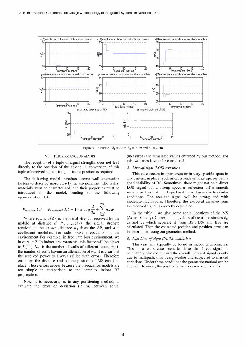
�Figure 5. Scenario 2:�� � ON�Q� �� � R��Q�"#��� � �S�Q
V. PERFORMANCE ANALYSIS
The reception of a tuple of signal strengths does not lead directly to the position of the device. A conversion of this tuple of received signal strengths into a position is required
The following model introduces some wall attenuation factors to describe more closely the environment. The walls’ materials must be characterized, and their properties must be introduced in the model, leading to the following approximation [10]:
TUVWVXYVZ�[� � TUVWVXYVZ�[:� � �5\ ]\ ^_` [[: �abX\ cX
de
Xf:Where TUVWVXYVZ�[�� is the signal strength received by the
mobile at distance d, TUVWVXYVZ�[:�� the signal strength received at the known distance [: from the AP, and ] a coefficient modeling the radio wave propagation in the environment For example, in free path loss environment, we have ]���2. In indoor environments, this factor will be closer to 3 [11]. gh is the number of walls of different nature,�bX\ is the number of walls having an attenuation of cX .�It is clear that the received power is always sullied with errors.� Therefore errors on the distance and on the position of MS can take place. Those errors appear because the propagation models are too simple in comparison to the complex indoor RF propagation.
Now, it is necessary, as in any positioning method, to evaluate the error or deviation (in m) between actual
(measured) and simulated values obtained by our method. For this two cases have to be considered:
A. Line-of-sight (LOS) condition This case occurs in open areas or in very specific spots in
city centers, in places such as crossroads or large squares with a good visibility of BS. Sometimes, there might not be a direct LOS signal but a strong specular reflection off a smooth surface such as that of a large building will give rise to similar conditions. The received signal will be strong and with moderate fluctuations. Therefore, the extracted distance from the received signal is correctly calculated.
In the table 1 we give some actual locations of the MS (Actual x and y). Corresponding values of the true distances d1, d2 and d3 which separate it from BS1, BS2 and BS3 are calculated. Then the estimated position and position error can be determined using our geometric method.
B. Non Line-of-sight (NLOS) condition This case will typically be found in Indoor environments.
This is a worst-case scenario since the direct signal is completely blocked out and the overall received signal is only due to multipath, thus being weaker and subjected to marked variations. Under these conditions the geometric method can be applied. However, the position error increases significantly.
0 5 10 15 2060
62
64x(A)variations as function of iterations number
iterations number
x(A
)
0 5 10 15 2055
60
65x(B)variations as function of iterations number
iterations number
x(B
)
0 5 10 15 2040
50
60
70x(C)variations as function of iterations number
iterations numbers
x(C
)
0 5 10 15 200
50
100y(A)variations as function of iterations number
iterations numbers
y(A
)
0 5 10 15 2058
60
62
64y(B)variations as function of iterations number
iterations number
y(B
)
0 5 10 15 2050
60
70
80y(C)variations as function of iterations number
iterations number
y(C
)
0 5 10 15 2055
60
65estimated abscissa of MS
iterations number
x(M
S)
0 5 10 15 2040
50
60
70estimated ordinate of MS
iterations number
y(M
S)
2010 International Conference on Design & Technology of Integrated Systems in Nanoscale Era
-5-
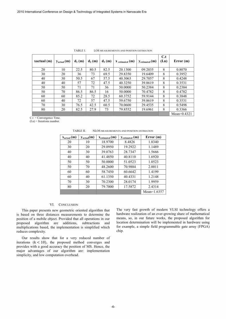
TABLE I. LOS MEASUREMENTS AND POSITION ESTIMATION
xactual (m) yactual (m) d1 (m) d2 (m) d3 (m) x estimated (m) yestimated (m) C.t
(I.n) Error (m)
20 10 22.5 80.5 82.5 20.1300 09.2035 8 0.8070 30 20 36 73 69.5 29.8350 19.6409 8 0.3952 40 30 50.5 67 57.5 40.3063 29.7057 8 0.4248 40 40 57 72 47.5 40.3250 39.8619 8 0.3531 50 50 71 71 36 50.0000 50.2384 8 0.2384 50 70 86.5 86.5 16 50.0000 70.4782 8 0.4782 60 60 85.2 72 28.5 60.3752 59.9144 8 0.3848 60 40 72 57 47.5 59.6750 39.8619 8 0.3531 70 30 76.5 42.5 60.5 70.0600 29.4535 8 0.5498 80 20 82.5 27.9 73 79.8552 19.6961 8 0.3366
Mean=0.4321 C.t = Convergence Time. (I.n) = Iterations number.
TABLE II. NLOS MEASUREMENTS AND POSITION ESTIMATION
xactual (m) yactual(m) xestimated (m) yestimated (m) Error (m) 20 10 18.9700 8.4826 1.8340 30 20 29.0950 19.2922 1.1489 40 30 39.0763 28.7347 1.5666 40 40 41.4850 40.8110 1.6920 50 50 50.0000 51.0523 1.0523 50 70 48.2600 70.9884 2.0011 60 60 58.7450 60.6642 1.4199 60 40 61.1350 40.4331 1.2148 70 30 70.2300 28.0174 1.9959 80 20 79.7000 17.5872 2.4314
Mean=1.6357
VI. CONCLUSION
This paper presents new geometric oriented algorithm that is based on three distances measurements to determine the position of a mobile object. Provided that all operations in our proposed algorithm are additions, subtractions and multiplications based, the implementation is simplified which reduces complexity.
Our results show that for a very reduced number of iterations (I 6 �5�, the proposed method converges and provides with a good accuracy the position of MS. Hence, the major advantages of our algorithm are: implementation simplicity, and low computation overhead.
The very fast growth of modern VLSI technology offers a hardware realization of an ever-growing share of mathematical means, so, in our future works, the proposed algorithm for location determination will be implemented in hardware using for example, a simple field programmable gate array (FPGA) chip.
2010 International Conference on Design & Technology of Integrated Systems in Nanoscale Era
-6-
REFERENCES
[1] Y. Zhao, “Standardization of Mobile Phone Positioning for 3G Systems,” IEEE Comm. Magazine, vol. 40, pp. 108-116, July 2002.
[2] H. Koshima and J. Hoshen, “Personal Locator Services Emerge,” IEEE Spectrum, vol. 37, pp. 41-48, Feb. 2000.
[3] J.H. Reed, K.J. Krizman, B.D. Woerner, and T.S. Rappaport, “An Overview of the Challenges and Progress in Meeting the E-911Requirement for Location Service,” IEEE Comm. Magazine, vol. 36, pp. 30-37, Apr. 1998.
[4] I. Jami, M. Ali, R.F. Ormondroyd, Comparison of Methods of Locating and Tracking Cellular Mobiles, Novel Methods of Location and Tracking of Cellular Mobiles and Their System Applications (Ref. No. 1999/046), IEE Colloquium, London UK,1/1-1/6.
[5] Y.T. Chan, K.C. Ho, A simple and efficient estimator for hyperbolic location, IEEE Transactions on Signal Processing, 42(8) (1994).
[6] Alba Pages-Zamora, Josep Vidal, Dana H. Brooks, Closed-form solution for positioning based on angle of arrival measurements, in: Proc. of the 13th Sym. on Personal, Indoor and Mobile Radio Communications, September 2002, vol. 4, pp. 1522–1526.
[7] Y. Zhao, Standardization of mobile phone positioning for 3G systems, IEEE Communications Magazine 40 (4) (2002) 108–116.
[8] C. D. Wann and H.C. Chin, “Hybrid TOA/RSSI Wireless Location with Unconstrained Nonlinear Optimization for Indoor UWB Channels,” IEEE WCNC, 2007, March 2007, pp. 3940–3945.
[9] Chi-Kuang Hwang and Kun-Feng Cheng “Wi-Fi Indoor Location Based on RSS Hyper-Planes Method,” Chung Hua Journal of Science and Engineering, Vol. 5, No. 4, pp. 37-43 (2007)
[10] Y. Chen and H. Kobayashi, “Signal strength based indoor geolocation,”in Proceedings of the IEEE International Conference on Communications (ICC ’02), vol. 1, pp. 436–439, New York, NY, USA, April-May 2002.
[11] R. Vaughan and J. B. Andersen, Channels, Propagation and Antennas forMobile Communications, ElectromagneticWaves Series 50, The Institution of Electrical Engineers, London, UK,2003.
2010 International Conference on Design & Technology of Integrated Systems in Nanoscale Era
-7-
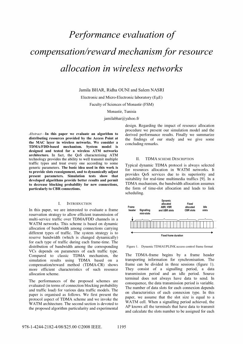
Performance evaluation of
compensation/reward mechanism for resource
allocation in wireless networks
Jamila BHAR, Ridha OUNI and Salem NASRI Electronic and Micro-Electronic laboratory (EµE)
Faculty of Sciences of Monastir (FSM)
Monastir, Tunisia
Abstract—In this paper we evaluate an algorithm to distributing resources provided by the Access Point at the MAC layer in wireless networks. We consider a TDMA/FDD-based mechanism. System model is designed and tested for a wireless ATM networks architecture. In fact, the QoS characterising ATM technology provides the ability to well transmit multiple traffic types and treat every one according to some generic parameters. The basic idea used in this work is to provide slots reassignment, and to dynamically adjust present parameters. Simulation tests show that developed algorithms provide better results and permit to decrease blocking probability for new connections, particularly to CBR connections.
I. INTRODUCTION In this paper, we are interested to evaluate a frame reservation strategy to allow efficient transmission of multi-service traffic over TDMA/FDD channels in a WATM networks. This scheme is based on dynamic allocation of bandwidth among connections carrying different types of traffic. The system strategy is to reserve bandwidth (which is changed dynamically) for each type of traffic during each frame-time. The distribution of bandwidth among the corresponding VCs depends on parameters of each traffic type. Compared to classic TDMA mechanism, the simulation results using TDMA based on a compensation/reward method (TDMA-CR) shows more efficient characteristics of such resource allocation scheme.
The performances of the proposed schemes are evaluated (in terms of connection blocking probability and traffic load) for various data traffic models. The paper is organised as follows. We first present the protocol aspect of TDMA scheme and we invoke the WATM architecture. The second section is devoted to the proposed algorithm particularity and experimental
design. Regarding the impact of resource allocation procedure we present our simulation model and the derived performance results. Finally we summarize the findings of our study and we give some concluding remarks.
II. TDMA SCHEME DESCRIPTION Typical dynamic TDMA protocol is always selected for resources allocation in WATM networks. It provides QoS services due to its superiority and suitability for real-time multimedia traffics [9]. In a TDMA mechanism, the bandwidth allocation assumes the form of time-slot allocation and leads to link scheduling.
Fixed frame duration
. .
. .
Frame header Signalling
mini-slots
Dynamic allocated ABR, VBR
and UBR slots
Fixed allocated CBR slots
Idle slots
Figure 1. Dynamic TDMAUPLINK access control frame format
The TDMA-frame begins by a frame header transporting information for synchronisation. The frame can be divided in three sessions (figure 1). They consist of a signalling period, a data transmission period and an idle period. Source terminal does not always have data to send. In consequence, the data transmission period is variable. The number of data slots for each connexion depends on characteristics of each connexion type. In this paper, we assume that the slot size is equal to a WATM cell. When a signalling period achieved, the AP knows all the terminals that have data to transmit and calculate the slots number to be assigned for each
978-1-4244-2182-4/08/$25.00 ©2008 IEEE. 1195
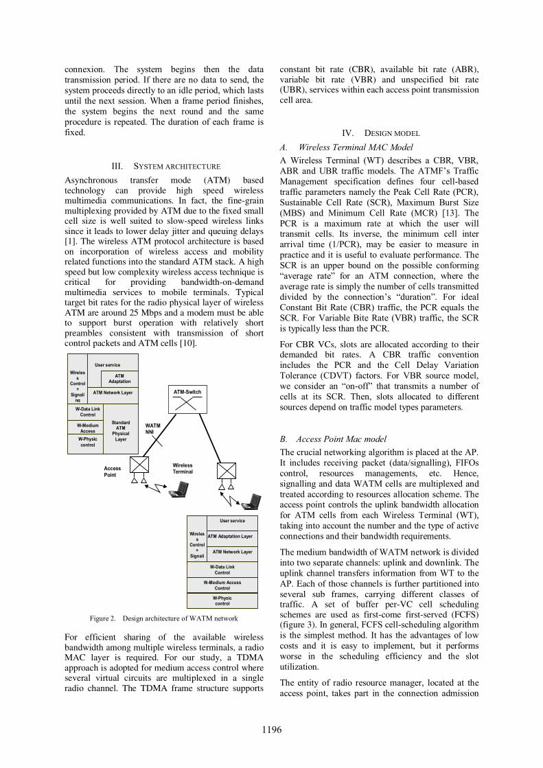
connexion. The system begins then the data transmission period. If there are no data to send, the system proceeds directly to an idle period, which lasts until the next session. When a frame period finishes, the system begins the next round and the same procedure is repeated. The duration of each frame is fixed.
III. SYSTEM ARCHITECTURE Asynchronous transfer mode (ATM) based technology can provide high speed wireless multimedia communications. In fact, the fine-grain multiplexing provided by ATM due to the fixed small cell size is well suited to slow-speed wireless links since it leads to lower delay jitter and queuing delays [1]. The wireless ATM protocol architecture is based on incorporation of wireless access and mobility related functions into the standard ATM stack. A high speed but low complexity wireless access technique is critical for providing bandwidth-on-demand multimedia services to mobile terminals. Typical target bit rates for the radio physical layer of wireless ATM are around 25 Mbps and a modem must be able to support burst operation with relatively short preambles consistent with transmission of short control packets and ATM cells [10].
Wireless
Control +
Signaling
W-Data Link Control
W-Medium Access
W-Physic control
Standard ATM
Physical Layer
User service
ATM Network Layer
ATM Adaptation
User service
ATM Network Layer
ATM Adaptation Layer
W-Physic control
W-Medium Access Control
Wireless
Control +
Signaling
W-Data Link Control
WATMNNI
ATM-Switch
Wireless Terminal Access
Point
Figure 2. Design architecture of WATM network
For efficient sharing of the available wireless bandwidth among multiple wireless terminals, a radio MAC layer is required. For our study, a TDMA approach is adopted for medium access control where several virtual circuits are multiplexed in a single radio channel. The TDMA frame structure supports
constant bit rate (CBR), available bit rate (ABR), variable bit rate (VBR) and unspecified bit rate (UBR), services within each access point transmission cell area.
IV. DESIGN MODEL A. Wireless Terminal MAC Model A Wireless Terminal (WT) describes a CBR, VBR, ABR and UBR traffic models. The ATMF’s Traffic Management specification defines four cell-based traffic parameters namely the Peak Cell Rate (PCR), Sustainable Cell Rate (SCR), Maximum Burst Size (MBS) and Minimum Cell Rate (MCR) [13]. The PCR is a maximum rate at which the user will transmit cells. Its inverse, the minimum cell inter arrival time (1/PCR), may be easier to measure in practice and it is useful to evaluate performance. The SCR is an upper bound on the possible conforming “average rate” for an ATM connection, where the average rate is simply the number of cells transmitted divided by the connection’s “duration”. For ideal Constant Bit Rate (CBR) traffic, the PCR equals the SCR. For Variable Bite Rate (VBR) traffic, the SCR is typically less than the PCR.
For CBR VCs, slots are allocated according to their demanded bit rates. A CBR traffic convention includes the PCR and the Cell Delay Variation Tolerance (CDVT) factors. For VBR source model, we consider an “on-off” that transmits a number of cells at its SCR. Then, slots allocated to different sources depend on traffic model types parameters.
B. Access Point Mac model The crucial networking algorithm is placed at the AP. It includes receiving packet (data/signalling), FIFOs control, resources managements, etc. Hence, signalling and data WATM cells are multiplexed and treated according to resources allocation scheme. The access point controls the uplink bandwidth allocation for ATM cells from each Wireless Terminal (WT), taking into account the number and the type of active connections and their bandwidth requirements.
The medium bandwidth of WATM network is divided into two separate channels: uplink and downlink. The uplink channel transfers information from WT to the AP. Each of those channels is further partitioned into several sub frames, carrying different classes of traffic. A set of buffer per-VC cell scheduling schemes are used as first-come first-served (FCFS) (figure 3). In general, FCFS cell-scheduling algorithm is the simplest method. It has the advantages of low costs and it is easy to implement, but it performs worse in the scheduling efficiency and the slot utilization.
The entity of radio resource manager, located at the access point, takes part in the connection admission
1196
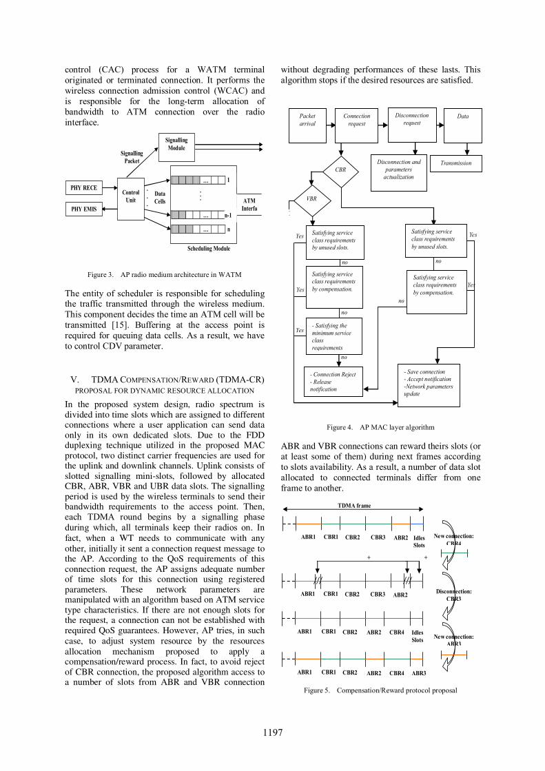
control (CAC) process for a WATM terminal originated or terminated connection. It performs the wireless connection admission control (WCAC) and is responsible for the long-term allocation of bandwidth to ATM connection over the radio interface.
. . .
Scheduling Module
Data Cells
n
1
Signalling Packet
Signalling Module
…
…
... ATM Interfa
Control
Unit
n-1 … PHY EMIS
PHY RECE
Figure 3. AP radio medium architecture in WATM
The entity of scheduler is responsible for scheduling the traffic transmitted through the wireless medium. This component decides the time an ATM cell will be transmitted [15]. Buffering at the access point is required for queuing data cells. As a result, we have to control CDV parameter.
V. TDMA COMPENSATION/REWARD (TDMA-CR) PROPOSAL FOR DYNAMIC RESOURCE ALLOCATION
In the proposed system design, radio spectrum is divided into time slots which are assigned to different connections where a user application can send data only in its own dedicated slots. Due to the FDD duplexing technique utilized in the proposed MAC protocol, two distinct carrier frequencies are used for the uplink and downlink channels. Uplink consists of slotted signalling mini-slots, followed by allocated CBR, ABR, VBR and UBR data slots. The signalling period is used by the wireless terminals to send their bandwidth requirements to the access point. Then, each TDMA round begins by a signalling phase during which, all terminals keep their radios on. In fact, when a WT needs to communicate with any other, initially it sent a connection request message to the AP. According to the QoS requirements of this connection request, the AP assigns adequate number of time slots for this connection using registered parameters. These network parameters are manipulated with an algorithm based on ATM service type characteristics. If there are not enough slots for the request, a connection can not be established with required QoS guarantees. However, AP tries, in such case, to adjust system resource by the resources allocation mechanism proposed to apply a compensation/reward process. In fact, to avoid reject of CBR connection, the proposed algorithm access to a number of slots from ABR and VBR connection
without degrading performances of these lasts. This algorithm stops if the desired resources are satisfied.
no
Yes
no
Yes
no
Yes
..
no
no
Yes
Transmission Disconnection and parameters
actualization
- Save connection - Accept notification -Network parameters update
no
Yes
- Connection Reject- Release notification
Packet arrival
Connection request
Disconnection request
Data
Satisfying service class requirements by unused slots.
Satisfying service class requirements by unused slots.
Satisfying service class requirements by compensation.
- Satisfying the minimum service class requirements
Satisfying service class requirements by compensation.
VBR
CBR
Figure 4. AP MAC layer algorithm
ABR and VBR connections can reward theirs slots (or at least some of them) during next frames according to slots availability. As a result, a number of data slot allocated to connected terminals differ from one frame to another.
TDMA frame
ABR1 CBR1 CBR2 CBR3 ABR2 Idles Slots
ABR1 CBR1 CBR2 CBR3 ABR2
+ +
Disconnection: CBR3
New connection: ABR3
New connection: CBR4
ABR1 CBR1 CBR2 CBR4 ABR2 Idles Slots
ABR1 CBR1 CBR2 CBR4 ABR2 ABR3 Figure 5. Compensation/Reward protocol proposal
1197
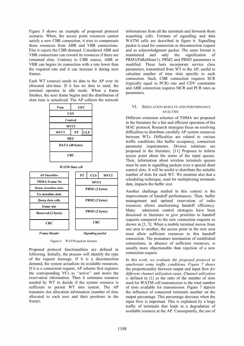
Figure 5 shows an example of proposed protocol scenario. When, the access point resources cannot satisfy a new CBR connection, it tries to compensate these resources from ABR and VBR connections. Else it rejects the CBR demand. Considered ABR and VBR connections can reward its resources if there are remained slots. Contrary to CBR source, ABR or VBR can begins its connection with a rate lower than the required rate and it can increase it during next frames.
Each WT (source) sends its data to the AP over its allocated slot-time. If it has no data to send, the terminal operates in idle mode. When a frame finishes, the next frame begins and the distribution of slots time is actualized. The AP collects the network
informations from all the terminals and forwards them acquitting cells. Formats of signalling and data WATM cells are described in figure 6. Signalling packet is used for connection or disconnection request and as acknowledgment packet. The same format is maintained and only the signification of PRM1(PaRaMeter1), PRM2 and PRM3 parameters is modified. These lasts incorporate service class parameters, transmitted from WT to the AP, useful to calculate number of time slots specific to each connection. Such, CBR connection requires SCR (typically equal to PCR) rate and CDV constraints and ABR connection requires MCR and PCR rates as parameters.
Frame Header
AP Identifier
TDMA Frame No
Down signaling slots
Up signaling slots
Down data cells
frame size
CRC
Reserved (2 bytes)
CLP
Type
CSN
Control
MVCI
MVCI
HEC
CRC
DATA (48 bytes)
GFC
PT
CLS
MVCI
MVCI
CRC
PRM3 (2 bytes)
PT
PRM2 (2 bytes)
PRM1 (2 bytes)
WATM Data cell
Signaling packet Figure 6. WATM packets formats
Proposed protocol functionalities are defined in following. Initially, the process will identify the type of the request message. If it is a disconnection demand, the system actualizes its available resources. If it is a connection request, AP scheme first registers the corresponding VCs as ‘‘active’’ and stores the reservation information. Then it estimates resource needed by WT to decide if the system resource is sufficient to permit WT into system. The AP transmits slot allocation information (number of slots allocated to each user and their positions in the frame).
VI. SIMULATION RESULTS AND PERFORMANCE ANALYSIS
Different extension schemes of TDMA are proposed in the literature for a fair and efficient operation of the MAC protocol. Research strategies focus on resolving difficulties to distribute carefully AP system resources between WTs. Difficulties are related to various traffic conditions like buffer occupancy, connection parameter requirements. Diverse solutions are proposed in the literature. [11] Proposes to inform access point about the status of the input queues. Then, information about wireless terminals queues must be sent in signalling packets over a special short control slots. It will be useful to distribute the suitable number of slots for each WT. We mention also that a scheduling technique, used for multiplexing terminals data, impacts the buffer size.
Another challenge studied in this context is the improvement of handoff performances. Then, buffer management and optimal reservation of radio resources allows ameliorating handoff efficiency. Many admission control strategies have been discussed in literature to give priorities to handoff requests compared to the new connection requests as shown in [3, 5]. When a mobile terminal moves from one area to another, the access point in the new area must allow sufficient resources to this handoff connection. The premature termination of established connections, in absence of sufficient resources, is usually more objectionable than rejection of a new connection request.
In this work, we evaluate the proposed protocol to ameliorate some traffic conditions. Figure 7 shows the proportionality between output and input flow for different channel utilization cases. Channel utilization is defined in [1] as the ratio of the number of slots used for WATM cell transmission to the total number of slots available for transmission. Figure 7 depicts the influence of connected terminals number on the output percentage. This percentage decrease when the input flow is important. This is explained by a huge traffic of terminals that leads to a degradation of available resource at the AP. Consequently, the use of
1198

an efficient resource allocated protocol is essential to avoid traffic performances degradation.
0
10
20
30
40
50
60
70
80
15 30 50 70 90
% input
% o
utpu
t
8 MTs35 MTs
Figure 7. Variation of traffic in function of terminals number
Moreover, TDMA-CR is a resource allocation protocol witch affect the connection reject probability. Figure 8 shows the effect of the proposed resource allocation protocol on the reject probability. It compares, for the same considered traffic scenario, a reject probability between classical TDMA and TDMA-CR schemes. We mention here that the big difference between the two cases at a first three seconds is explained by the great effect of compensation method. In the remained simulation time, the difference of reject probability variation between the two methods becomes small. This result is justified by the limit of resources compensation for each traffic class. This means that the efficiency of a proposed scheme can decrease when resources are limited or a great number of terminals need to be served.
0
0,05
0,1
0,15
0,2
0,25
0,3
0,35
0,06
0,68 1,
31,
912,
533,
163,
79 4,4
5,03
5,64
6,27
6,89
7,51
Time (sec)
Rej
ect p
roba
bilit
y
TDMATDMA-CR
Figure 8. Connection reject probability
Results presented by figure 8 show that a compensation mechanism does not decrease a reject connections number only, but it also increase the percentage of resources utilisation as shown in figure 9. The improvement of resources utilisation explains that compensation approach avoid resources wasting and increase a number of served connections. In fact, if compensation method decreases the number of rejected connections, it means that this method allows connecting new terminals with remainder and compensated resources.
0
10
20
30
40
50
60
70
80
90
1 2 3 4 5 6 7 8
time (sec)
%in
put
TDMATDMA-CR
Figure 9. Resources utilisation percentage
0
0,1
0,2
0,3
0,4
0,5
0,6
00,
280,
560,
831,
12 1,4
1,67
1,95
2,23
2,51
2,78
3,07
3,34
3,62
Time (sec)
CDV
(ms)
TDMATDMA-CR
Figure 10. CDV of CBR connection
The cell delay variation (CDV) is a QoS parameter which depends on the type of service class. CDV should take on almost constant value especially for CBR classes. Figure 10 compares a cell delay variation (CDV) of CBR connection using classical and modified TDMA method. We conclude that a modified TDMA scheme let CDV more stable. It gives a sufficient resources distribution strategy that arrange all connections in an equilibrium way.
VII. CONCLUDING REMARKS It is necessary to provide QoS guarantees subject to ensuring delay constraints, prescribed data rate and loss for the various applications such as voice, video and high quality multimedia services. The MAC is necessary for QoS based bandwidth allocation to multiple ATM traffic classes. In this works, we have proposed an approach to support wireless multimedia applications using TDMA/FDD MAC protocol based WATM. The design algorithms use TDMA/FDD-based access scheme, with a compensation/reward process. The TDMA mechanism traits all signalling information of connected terminals and executes the suitable process to compute the allocation of slots in next frame. Simulation results show the efficiency of such compensation/reward process to ameliorate traffic condition. We mention that this algorithm can be adopted for others networks protocols.
1199
REFERENCES [1] Ekram Hossain and Vijay K. Bhargava; Link-Level Traffic
Scheduling for Providing Predictive QoS in Wireless Multimedia Networks; IEEE TRANSACTIONS ON MULTIMEDIA, FEBRUARY 2004, VOL. 6, NO. 1.
[2] Xiaohua Li; Contention Resolution in Random-Access Wireless Networks Based on Orthogonal Complementary Codes; IEEE TRANSACTIONS ON COMMUNICATIONS, JANUARY 2004, VOL. 52, NO. 1.
[3] parameswaran ramanathan, Krishna M. sivalingam, prathima agrawal and shalinee kishore; Dynamic resource allocation schemes during handoff for mobile multimedia wireless networks; IEEE journal on selected areas in communications, July 1999, VOL XX.
[4] Bih-Hwang Lee Hsin-Pei Chen Su-Shun Huang; Dynamic Resource Allocation for Handoff in WATM Networks; Proceedings of the 2005 11th International Conference on Parallel and Distributed Systems (ICPADS'05) IEEE 2005.
[5] Maria C. Yuang, Po L. Tien, and Ching S. Chen; A Contention Access Protocol with Dynamic Bandwidth Allocation for Wireless ATM Networks; IEEE 2000, p149-153.
[6] D. Raychaudhuri, L.J. French, R.J. Siracusa, S.K. Biswas, R. Yuan§, P. Narasimhan & C. Johnston; WATMnet: A PROTOTYPE WIRELESS ATM SYSTEM FOR MULTIMEDIA PERSONAL COMMUNICATION; IEEE J. Selected Areas in Communications, Janvier 1997, pp.83-95.
[7] Tarek Bejaoui1, Véronique Vèque, Sami Tabbane; Combined Fair Packet Scheduling Policy and Multi-Class Adaptive CAC Scheme for QoS Provisioning in Multimedia Cellular Networks; International Journal Communication System 2005; Copyright 2005 John Wiy & Sons. Ltd.
[8] Jaime Sánchez, Jorge Flores Troncoso, José R. Gallardo; RETRANSMISSION ALGORITHM BASED ON POWER PRIORITIES FOR WIRELESS NETWORKS; PIMRC 2002; IEEE2002.
[9] Celal Ceken, Ismail Erturk, and Cuneyt Bayilmis; A New MAC Protocol Design for WATM Networks; ADVIS 2004, LNCS 3261, pp. 564–574, 2004; Copyright Springer-Verlag Berlin Heidelberg 2004.
[10] H. KIM, S.K. BISWAS, P. NARASIMHAN, R. SIRACUSA and C. JOHNSTON; Design and Implementation of a QoS Oriented Data-Link Control Protocol for CBR Traffic in Wireless ATM Networks; Wireless Networks 7, 531–540, 2001; Copyright Kluwer Academic Publishers 2001. Manufactured in The Netherlands.
[11] Rolf Sigle, Thomas Renger; Fair Queueing Wireless ATM MAC Protocols; Computer Networks 31(9-10): 985-997 (1999)
[12] Wojciech Burakowski, Halina Tarasiuk, Andrzej Beben and Marek Dabrowski; EuQoS IST project: Overview of the QoS framework for EuQoS; IST-1999
[13] Peter Sholander, Luis Martinez, Lawrence Tolendino, Bruce A. Mah; The Effects of User Mobility on Usage Parameter Control (UPC) in Wireless ATM Systems;
[14] Michael Wolf, Rolf Sigle; Medium Access in Wireless ATM Systems for Industrial Applications: Requirements and Solutions, Proceedings of the 1998 IEEE International Performance, Computing, and Communications Conference, p18-22, ISBN: 0-7803-5794-9.
[15] jongho bang, sirin tekinay, nirwan ansari; A novel capacity maximisation scheme for multimedia Wireless ATM systems providing QoS guarantees for handoffs; VTC2000, copyright IEEE2000.
Author biography
Jamila Bhar- received her Engineering diploma in Electric and her DEA in Communication system from the National School of Engineering of Tunis (ENIT), Tunisia in 2001 and 2002, respectively. Currently, she is a PhD student. Her research interests include protocol adaptation in heterogeneous networks, traffic
management and Quality of Service for high speed networks. Her recent work has been in traffic control in WATM network.
Ridha Ouni- received his doctoral degree in physic (2002) from the Science Faculty of Monastir, Tunisia He is currently an assistant Professor at the Preparatory Institute of Engineering Study of Monastir (IPEIM), Tunisia. His research interests include computer networks, flow and congestion control, interoperability and performance evaluation. He is interested in many areas of hardware/software protocol verification and design for distributed systems.
Salem Nasri- received his Doctoral degree in automatic control and computer engineering from the National Institute of Applied Sciences of Toulouse France, in June 1985. His research interests are in the fields of computer networks, communication systems and multimedia applications. In May 2001 he obtained the diploma of “Habilitation universitaire”. Since then he has been a professor. He developed collaboration with many laboratories in France such as LSR (Grenoble), CRAN (Nancy), and some other laboratories in Tunisia. Currently he is a professor in the Computer Science Department, Qassim University in the Kingdom of Saudi Arabia.
1200
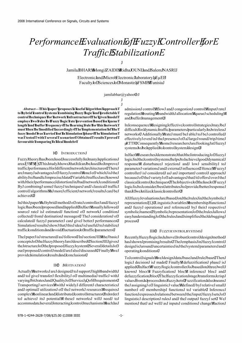
����������� ���������������������������������������������������
�
����������� �������������������������������������
��������������� ������������������ ������!�"�#�$�%��&��!��'��������(��'� ���(����"%� $��)&��(���
*����� ���+!����,'����
���������������������������� �� �� ���������������������������������������������������� ���� �������������������������� ������ �� ���� ������� ������� �� ������ ���������������������� ������� ������������������������������ ����������� ���� ��� �������� �������� �� ���� ������������� ��� ���� �� �������� ������������ ��� ������������ ��� ���� ������������������� �������� ����������������� ��������� ����� ����� ����� ��������� ������� �� ���� ��������� ���������������������������
�,� ��)����-)����%&..!������!���(� ����&(���(&���(('&��!�������!��//��������(������01��2��34,�)��(�(�&�!�(��5(������������� ��&(��������/��6�����''���/��'�������� '�����''������ ���5��7����������&��(,�)��������� ���!� ��6������(� �'� '&..!� ��������� ���� �'� 5����� �(� ����� ����!� ��� ������� ��/����(�� ����,� 8���� ��� ���''��(� ���� 7��5��5���� ������ /��'�������� ��(�������� ��� ��� ���5��7� ���������(,��!� ��� ������ (���� '&..!� ������9&�(� ���� ���((����� ���''����������� ���������(�� �� ����� �''������� ���5��7� ��(&��(� ���� �������6��,��
��� ���(� /�/���� �� �! ���� ������� �'� ����� ����������� ���� '&..!���������(� ����/��/�(��������//����,����'�����&(&���!�����5���(�&���� ����� �(� �(�������� '&������� �'� ���5��7� �������������������� '���� ��(��������� ��((���(,� )��� ���(���������� �'�����&������ '&..!� /��������� ���� ��6�� ������ /��'�������(,����&������� ��(&��(� (��5� ����� ���(� ����� �(� &(�'&�� ��� (�� ���.�����''������������(������6����'�&��&�������'����''���/��������(,�
)��� /�/��� �(� (��&��&���� �(� '����5(,� ��� (������� ���� ���� �(��������/�(� �'� ���� '&..!� �����!� ���� ��(��� ��,� �������� ���� ��6�(�����(��&��&����'� ����/��/�(���'&..!�(!(���,���6�����������(��'��&�� /��/�(��� �������� ������ ���� ��(�� ��(�&((��,� %�����!�� 5��/��6����(��&���������(&��(����������&(���(,�
��,� � �)�8)������&���!�� ���5��7(� ���� ��(������ ��� (&//���� ����� ���5��������� ��� ��6�� ����('��� '��:� ����!� �'� �&��������� ���''��� 5����6��!���� ��� ����(� ����;&����!� �'� ���6���� ";��$� ��9&�������(,�)���(/������� (��6���(�� 5���� 5����!� ��''������ ����������(���(����� �/������ &����.������ �'� ���� ���5��7� ��(�&���(�� ��9&���(����/��:������������������(��� &������������(��&��&��(,������������� �����6�� ��(� /���������� ���(�� ���5��7(� 5���� ����� ���������������(�6��������������������������������(�(��(&����(�
����((���� ��������� '��5� ���� �����(����� ��������� ��/&�� ��������&�������� ��&������ ���5����� ������������ 9&�&�� (����&���������� &''�������������,��
������(�9&��������(��������''����6����������(��������(���!� ����''��&���'����!���������''���/��������(�/�����&����!����5�����((����5��7(,� ����������!�� ����� �&(�� �� � ��� ��� �� ������������''����6��!� �6��� ��� ���� /��(����� �'� �� ������ ��&��� ���/� �����"�))$,� -��(�9&����!�� (���� ��(�������(� ���� ���7���� ��� '&..!�(!(���(���� ���//����������������(!(������(���,��
��� '�������(������(������(������ ����� ���� ������&������'� '&..!������� ��� ������������(!(���(����/(� ��������6��������!����������(/��(��� ��(�&� ����� ��*������� ���� ��5� (��(� ����!� ���/��������� 6��������(� ���� �:������� ��'�&����(,� ������ %&..!������������ �(� ���(������� �(� ��� ��/������� �������� �//������ ���&(�� �'� ���� 6�����!� �'� ��6������(� ����� ��� �''��(� �6��� �������((�������������������9&�(,�)���� *����6���'�����&(���'�%&..!������� �(� ��� ���(����� �(�� ����� &��(� ��� /��6���� ������ ��(/��(��������'�5��&����.�����((�������������,��
��� '&..!� �6��&�����(� ���� �(��� ��� ���� �&��(� ��� ���� (!� �������/��(���������0<4,�=���&�(����6���� ��(����� ��(��/�'&������(����� '&..!� �/�������(� ���� ��'�������� !� ������ ��(/����6��(!� ����� ����(,� �!� ����� ��/��(��������� �'� ���� �&��(� ����5(���(!� &����(���������'� ���� �&��(� ���� (��/��'��(� ������ &������/����((,�
���,� %���>�-��)��=��>�)� ���������!�'&..!��������(�����6����� &(������������(�������������(� (��5�� /����(���� ��(&��(,� )��� ��/��(�(� ��� '&..!� ����������(���� �(� ���&��� &�����������(� ��� ���� (!(���� /��������(� �����/�����������������(,�
)�� �������� (�����(�� 5�� ��(���� ����� �(�� ���� �&��� �(�,� )���������� ����(���� �(� ����,� %�����!�� ��'&..�'�������� /��(�� �(��//����,� ���'�����%&..!� ����������������� �(� �(������ ������5����7��5�� ���(?� %&..!'�������� ����� ��'������� ���� ������'&..!'�������� ���,�)���'&..!'��������(���������('���(����(/�6��&�(�'������/����((������'&..!�(��(,�%&..�'����������(������(����� �((������� �'� ����&�(���� 6��&��� ��'����� !� ������6�� (������&� ��� �'� ��� ��(��/� '&������(� ��� 6���� ��,� ��'�������'&������� �:/��((�(� ��������(� ��5���� ���� ��/&�� '&..!� (��(� �'�����&�(���� ��(���/����� �&��(� ���� ���� �&�/&�� '&..!� (��,� @���������� ����� �(� 5���� �(� ��/&�(� ���������(� �������� �������
2008 International Conference on Signals, Circuits and Systems
978-1-4244-2628-7/08/$25.00 ©2008 IEEE -1-
������������ '��� ���� �&�/&�(� �&(�� �� � (��6��,��5�6���� ���� %&..!� �&��� �(�(� ���� ���&����� '���� ������������ (������!,� )��!� ���� '���&������ !� �� (�������� �(?��'� ���������� )���� ����(���,� )����� ���� (�6����� ������(� �'���'������� ��� ���� �������&��?� �:������ ��:�/���� ��� (&��/������&��(,� ���� ���� ������� ��� ���!� ���� �&��,� ��6����� ����&�(����6���� ��(� ������&��� ��� ���� ��� �/������(,� )�����'&..!'�������� (����� ����('���(� ���� '&..!� (��(� ��� ���� �&�/&��(/������������(/���������(�����(,�
������������������������(�����(������5�&��� ����((�(��(���6�����/��������� 6��������(� ����� ������������ ����������(�� 5�� ���(��������� �! ���� ����������� (��&��&��� (��5�� ��� %��� <,� @�� ���A�����(������������(5�������� ��5���������5��������9&�(�� &����(���� �������,� )��� �''������!� �'� ���(� �//������ �(� ����� '��� �����''��� ����������.��� !� '�(�� ��������� ���������(� ����'�&��&�����(���(�(,�
�8,� ����B���%�C��C�����%���>�-��)��==����
)��(� /�/��� /��/�(�(� �� �� &(�� '&..!� ����������� '��� �&�/&�����&������� ���''��� ����,� ��(��� ��� ���� ������&���� ����������(������� ��������� ����� ���(�(�(� �'� ��� ������ '&..!� ���&�������������(&��������,�%���D�(��5(���5����� ������&�/&������,��!�(&/��6�(���� �'� %�%�� ���&/���!� ���� ��(� '������� '��9&���!��%&..!� ��������6�(� (!(���� ��/&�(,������ ����&�(���� 6���� �����(������ �����!��&� ����'��((����������� ��(��/�'&������(?��������� ��(��/� '&������� �(� ��/��(������ !� �� ��������,� )����������� ��(��/� '&������(� ����5� (��/��� ��/������������ �'� ������(�� 5����!� &(��� '���(?� ����������� ��������� ���� ���/�.���,��&�/&�� ��� ��(��/� '&������� 5�(� �:/��((��� ��� ���� '&..!�(��������(,��
�
� ��������������
!������������
� ��������������������
�"�
�
%��&���<,�� ! �����������������
�
#��������� ��������
� ����� ���
!������������
� �� ���
$�� �������������� ����
�$����������
� �����������
�%� �����������
�$������
�
%��&���D,�� C��/�(���%&..!������������(������
�
)�=���,�� =��B���)�-���=���
������������&�
������ �����
������� ����� � �� ����
�������������������
����� 6��!�(������ (������ (������ ������� �������
������ (����� (������ ������� ��5� ��5� �� ������ ��5� 6��!���5� 6��!���5� 6��!���5
�%&..!�����&�(��������(��'���/&�������&�/&��6���� ��(�����(��5�����'���1��E�����2���(/����6��!,�)���6��&�(��'�'&..!���� ��(��/�'&������(� /��������(� 5���� �((������ ���� ��'����� ����&���/���������!����/&����(��&������,�%&..!��&��(�/������/������ ������(����������������������/���������)� ���<,�
��� ������ ��� �������.�� ����&�(���� 6���� ��(�� 5�� /������� ��� ����'����5����5�!,��'�����6���������'������'���������!�6���� ���F!G��(�0��� 4��������� �����6���������0�<��<4�&(��������'����5�������������������?�
������
−−−
=D
�
)��� ������&���� ���� ���/�.������ ��� ��(��/� '&������(� �������������!�� (�������� 5���� ���� ��'����� 6��������� '����� �'� �����(!(��������!�"D�H<$,������� ��'�:�������������!,����� ���(� 5��7�� 5�� ���(����� �(� /���������!� ����� ���� %�%���6������ 6��������� ���� ���� '������� '��9&���!,� )��(�� ��/&��/��������(�5���� ��&(����(�����&�(����6���� ��(,�)�����6���������(����(������:/��������������'����5����'��&��(?�
%�%�?�"��/�!����������'&��$�
��
'�(�)�*(�*'�
� �������� ������
+,�-�
�
%��&���1,�� %�%������&�(����6���� ���
%������� '��9&���!?� ""�$'�(�� ���&������� " $(��5� ���&�������"�$�&����"�$(��5�������(���"�$'�(��������(�$,�
�
��
*(� *(./�*(./� (� (./�)./�)�
+,�-�
,�-�,�-�,�-�,-� ,-�
�%��&���E,�� %�������'��9&���!�����&�(����6���� ���
��������&�/&�����������������(���������������������'�6��6�����������6��(��(?� "6��!� ��5� "<$�� ��5� "D$��������� "1$�� (������ "E$��6��!�
2008 International Conference on Signals, Circuits and Systems
-2-
(������ "2$$,� %��� 2� ���&(�����(� ���� 6��������� �'� ���� �&�/&������&�(���(�6���� ��(,�
�,0-�,'-�,(-� ,/-�,1-�
�%��&���2,�� �&�/&������&�(����6���� ���
)���/��/�(���'&..!�������������/��!(� ������&���(,� �)��� '��(��(����� �(� &/������ �'���� �6��!� �����6��� ),� )� �(� ������� ������������� (���,� ��� ��/��(���(� ���� ����� �����6��� ��5�������(��&��6��'��� ��7(,����(��&��� ��/��/���!����(�������������������(�������/��������(,�)����� ���((&����5����(��&������(��:/�������(,� ��� ��������(� ���� ��������� �'� �5�� /��������/����((�(,� ��� '����� �&����� ���� '��(�� (������ '&..!� ��������������&����(� ����&�(���� 6���� ��(� ���(������� ��� ���(� 5��7?� %�%���6������ �����������%�%��'�������'��9&���!,�'�����������.�������(�� 6���� ��(�� ��� ��'���(� ������ �((�������� ��� ��(��/�'&�������"������������$,���
� �2�������3�����������
3�� ����$�������������,&-�
3�� ����$�������������� ����,�-�
��������4�5�
�����:
��:����
D��
����−
−−×= �
��������4&5�
�����:
��:����
D��
����−
−−×= �
����(6�6/�3�� ���+�,��-�
����(6�60�3�� ���+�,&�-�
����(6760�3�� ���������������������� ������� ����� ��������8�9��������
�3�� ���:���� �������������
������
��
=
== 2
<
2
<
�
!�
�
"�" �
3������!���
��
%��&���I,�� %&..!�������������������
� (������ (����� �(� �(��� ��� ���� ��:J���� ������ ��� �//�!���'������� '&������(,� ��� �(� �(��� ��� ����!���� �&�� ���� �/���������� !� �����&�� ��5,� )��� �/������� ��� �(� �������� �&�� !���:��&����5,�������(�9&������5��� ���������(�����6��&�(��'������&�/&��6���� ������ ��(�������������'&..�'��������(����,���'&..�'�������� /����((� �(� &(��� ��� ���/&��� ���� '����� '&..!��&�/&�� %��� I� (��5(� (���� ������(� �'� ���� ��6���/��� '&..!����������,��
8,� �� �=)��������=)���������(�/�/����'&..!� �������(��//�����5�������"6���� �����������$� (��6���� ���5�����((�) �"@) $����5��7,�)������(��6���� ��6���/��� '��� ) � ���5��7� ����� ��� �� ������������'��� &(�� ���5�����((�) ���6��������� 0<K4,� �������� ����������(&//��������!����(������(�(&����(�������''��&��!����/��������������''��� ����������(���(� '��� �� ���� ��������(�� ���5����� ��((���&(��� !�����(&//��������!�'����(���������������������'�������/���������� ���� ��/������� ��� ������ ����� ��� �� 5�����((��������,�%��� ���(�� ���(��(����� ���/��6����&��'�����!��'������������9&����!��'�(��6����";��$��&�������(� !�5�����((�) ������ /��(������ 5��7� '��&(� ��� ���� ��6���/����� �'� �� �� &(�����/��6�� �����(����� �������� ���������� ��� @�����((� ) ����5��7(,����� '����� -�� "���5��� -���� ����$� �(� ����������� !� ����� �������� �'� ���((����� ��� �(��������� ���� '&..!� �&�/&��/��������,� )��� /��/�(��� �! ���� '&..!� ������ ����������� �(���(��� ���&(����8�=�����&���,��/���'�����6���/���/��7���(�����/�((� ������6��(�����'������6���� ��(�����������������'�������� ����(���������(������������((���(,��
�%���3�(��5(�/��������(�� �������'��������''���(�������,�;�����%� ��/��(���� ���(&���� ����&�(���� 6���� ��(,� )��� ����������� �'�'&..!��&��(���/���(����������<2���� �������(�"(����� ���<$,�)����//����������'���:��&���/���������6�(�2�5�����(�"/<��/D��/1��/E� ���� /2$,� %�����!�� ��'&..�'�������� (����� ����&����(� ��������������� �(���������������������,�
�
%��&���3,�� ���&������%&..!�/��������(�
2008 International Conference on Signals, Circuits and Systems
-3-
)�� �6��&���� ���� ��6���/��� '&..!� �������� ����������� 5�����(����� ��6��(�� ���''��� ���������(� '��� 5�����((� ) � ����(,�)���(�&��������������(���'��������������������(������������������� ���''��� '��5����������(����������������������,�%���L�(��5(�(��&������� ��(&��(� �'� ���� '&..!� �! ���� ����������,� ��������(�����(� ����� ���� ��6���/��� ���������� �&�������(� ����&����������������(������!������(�� ���.�(����''������������(������6���(� '�&��&������ �'� ���''��� /��������(,� -��/������ ��� -��6��������� �(�������� !� ���((����� ��� (��6���� "'��� M$�� ����/��/�(���'&..!�������������6�(�������''���������(&��(,����'���������'&..!��! ��������������������/�(����(�� ���.������-�����������������������"�:/����������$����'�&��&��������''������������(,��
�
�
�����
�����
�����
�����
�����
����
����
���
����
����
�����
�����
�����
���
�
�����
�����
� ��
� ��
� ��
� ��
�������
�� ��������
����
�
%��&���L,�� -���������6���������'���%&..!��! ���������������
�
�����
�����
�����
�����
�����
����
����
���
�����
�����
����
���
����
���
�����
����
� ��
� ��
� ��
� ��
� ��
�������
�� ��������
����
�
%��&���M,�� -���������6���������'������((��������(��6����
�
�����
�����
�����
�����
�����
����
����
���
����
����
���
����
����
� ��
� ��
� ��
� ��
� ��
� ��
� ��
� ��
� ��
�������
�� ��������
����
�
%��&���<K,��-���������6���������'���8�N8�����(��6����
�
�����
�����
�����
�����
�����
����
����
�����
�����
����
����
���
����
����
�����
�����
����
����
����
�������
�� �������� ������������
������������������� �
�
%��&���<<,������6�����'������6(������
��(&��(� �'� /��/�(��� '&..!� ���������� ���� ��(�� ���/�����5����8�N8�� "8���&��� ��&���N8���&��� ��(��������$� �����/�,� 0<K4�(��5(������8�N8��������(�� ���(�(�(�&����������(����(�9&������'� �������� ���/� ���&�����,� %��� <K� ���&(���(� ���� �''���� �'�������/���/����!����-��6��������,��5�6���� ������/����!��'� ����������������(����������������������'�&��&�����,�%��� <<� �:/����(� ���� -�� 6��������� '��� ���� ������ ��(�(�"-��((����� ��� (��6����� 8�N8�� �����/�� ���� �! ���� '&..!�����������$,� )��(� '��&��� �����(�����(� ����� /��(� �'� ����� ������(/������ ���� '�&��&�����(� (����� ������������ �����6��� '��� -��6���������&(����%&..!�����������,�
8�,� -��-=������)��� ����� � *����6�� �'� ���(� 5��7� �(� ��� ��6���/� �� �! �������5��7������������������(�� ��������*&(�����''�������,�����(� �(������ ��(� �5�� /��������(� ���� �6��� ��� ����� 6��&�� ��6��� !����((����� ���''�������������,�)��(��! ����(!(����5������������������ ���� ���5��7� ���������&��� ��� 5����� ��� 5��7(�� (���('!� ���''���(�� ���.�����,����'�����������6���/����������������������(��� &(�� ���&(�� ��� ���� �� ���/���� ��� ��''������ ���5��7� ���������&��,����&������� ��(&��(� ��6�� �����(������� ����� ���� �! ���� '&..!��������������6�(�(���('�����!�/��'�������,��
��%����-���0<4� �����(&���B�����������>&���=�O�������/����%&..!���'�������
C����((��� 5���� �!������ ���!(�(� ���� �����&����� -�/� ������(O� ���-��)���(,���',�����!(�,��8�=��LL�������<K��/DE<K�DE<I������ ���DKK2�
0D4� �,�,�)����������,�����(����O���(�����'��� &(��%&..!�=�����C�5����!(���� ��� ���.��O� PP�,� �������������� -��'������� ��� -��/&����������������������!(���(�������������������������O�-�����DKK3��Q�DKK3�@��),��B�
014� )&��������� -��B�� -���������� -���� �#� C����� =��O� �� &(��%&..!� ��������� ���&������ ��(���� '��� �� -��((� �'� ''���� �����������!(���(O����-��)���(,�%&���������(��8�=��LMR�����E��C��=�DKKI�
0E4� S�&��-����� S@S�� �#� �����5�� S� $� ��/��6�� ��&���%&..!����5��7(�5������������'�%&..!�B���&������O����-��)���(,���',�T��!(�,��8�=��LLR������M����C)� ����DKK2�
024� ,� ����7���� ���� �,� -��7��&�O��(���� ���� ��/������������ �'� �� ! ����%&..!� -���������� '��� �� ����C��'�������� ���&������ ����O������������������&������'�//����� ���������(�����-��/&�����������(��8�=�E�����D��DKK3������<1K2�21<1�
0I4� =������� =,� ,� ����@� ���� S��� �&�(����� ��/��6���� ������ &(���((��'�%���>�������) �����������������'�����������&������/�����(O� ��������������� -��'������� ��� ������������ ������� C����((���� ����-���&��������(�� �� �&�����&(����������6�<MML�
2008 International Conference on Signals, Circuits and Systems
-4-
034� %�����..���������������������������.6�O�%&..!�)�&(�� '���C�������C���� ��(��� �!(���(O� C���������(� �'� @����� �����!� �'� �������������������������)��������!��8�=�D<�� >�DKK3������<1K3�ILLE�
0L4� ����'����� B���5���O� ����������� %&..!� -������,� � �&�6�!� �'� ��������������(&��(O�=����� ��&������'� ���� �BC=��8�=�<1�����2��/2D2�2E<��DKK2�
0M4� *���� �������� ��6�� ���� �� ����(��� )����(��� ����� >���� ���O� ���-���?���(��� &���� (�'�� ���/&����� ����&(�������������� (!(���O� ��&������'����5��7�����-��/&����//��������(��8�=�1K��/L<RML��DKK3,�
0<K4� ������� ���� ������ ������ ��������� �==��� ������ ����O���/��6�����(� �'� ���� ��� ���/� /��'�������(� ��� �� 5�����((� ) ����5��7O� /���������� �'� � �������������� -��'������� ��� ��������������(�"�- $��8�=�I�����L��/DM2�DML�����,�DKKE,�
��
2008 International Conference on Signals, Circuits and Systems
-5-
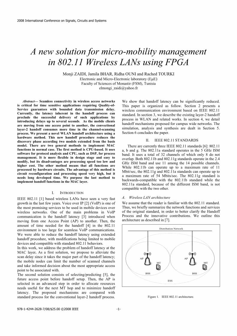
A new solution for micro-mobility managementin 802.11 Wireless LANs using FPGA
Monji ZAIDI, Jamila BHAR, Ridha OUNI and Rached TOURKIElectronic and Micro-����������� ������������)Faculty of Sciences of Monastir (FSM), Tunisia
Abstract— Seamless connectivity in wireless access networks is critical for time sensitive applications requiring Quality-of-Service guarantees with bounded data transmission delay. Currently, the latency inherent in the handoff process can preclude the successful delivery of such applications by introducing delays up to several seconds. As the mobile clients are moving from one access point to another, the convectional layer-2 handoff consumes more time in the channel-scanning process. We present a novel WLAN handoff architecture using a hardware method. This new handoff procedure reduces the discovery phase according two models extended from the basis model. There are two general methods to implement MAC functions in normal case. The first method is CPU-based. It uses software for protocol analysis and CPU, such as DSP, for process management. It is more flexible in design stage and easy to modify, but its disadvantages are processing speed too low and higher cost. The other method means that all functions are processed by hardware circuits. The advantage of this method is circuit reconfiguration and processing speed very high, but it needs long developed time. We purpose the last method to implement handoff functions in the MAC layer.
I. INTRODUCTION
IEEE 802.11 [1] based wireless LANs have seen a very fast growth in the last few years. Voice over IP [2] (VoIP) is one of the most promising services to be used in mobile devices over wireless networks. One of the main problems in VoIP communication is the handoff latency [3] introduced when moving from one Access Point (AP) to another. Then, the amount of time needed for the handoff [4] in the 802.11 environment is too large for seamless VoIP communications. We were able to reduce the handoff latency using extended handoff procedure, with modifications being limited to mobile devices and compatible with standard 802.11 behaviors.In this work, we address the problem of handoff latency at the MAC layer. As a first solution, we propose to alleviate the scan delay since it takes the major part of the handoff latency;the mobile nodes can limit the number of scanned channels and take informed decision about the most appropriate access point to be associated with.The second solution consists of selecting/predicting [5], the future access point before handoff setup. Then, the AP is selected in an advanced step in order to allocate resources needs useful for the next MT hop and to minimize handoff latency. The proposed mechanisms are compared with standard process for the conventional layer-2 handoff process.
We show that handoff latency can be significantly reduced.This paper is organized as follow. Section 2 presents a wireless communication environment based on IEEE 802.11 standard. In section 3, we describe the existing layer-2 handoff process in WLAN and related works. In section 4, we detail handoff mechanisms proposed for campus wide networks. The simulation, analysis and synthesis are dealt in Section 5. Section 6 concludes the paper.
II. IEEE 802.11 STANDARDSThere are currently three IEEE 802.11 standards [6]: 802.11
a, b and g. The 802.11a standard operates in the 5 GHz ISM band. It uses a total of 32 channels of which only 8 do not overlap. Both 802.11b and 802.11g standards operate in the 2.4 GHz ISM band and use 11 among the 14 possible channels. While 802.11b can operate up to a maximum rate of 11 Mbit/sec, the 802.11g and 802.11a standards can operate up to a maximum rate of 54 Mbits/sec. The 802.11g standard is backwards-compatible with the 802.11b standard while the 802.11a standard, because of the different ISM band, is not compatible with the two other.
A. Wireless LAN architectureWe assume that the reader is familiar with the 802.11 standard. Thus, we briefly summarize the network functions and services of the original standard, in order to better clarify the Handoff Process and the innovative contributions. We outline thisarchitecture as described in [7].
ESS
BSS BSS
Distribution Network
AP AP
MT MT
Figure 1. IEEE 802.11 architecture.
2008 International Conference on Signals, Circuits and Systems
978-1-4244-2628-7/08/$25.00 ©2008 IEEE -1-
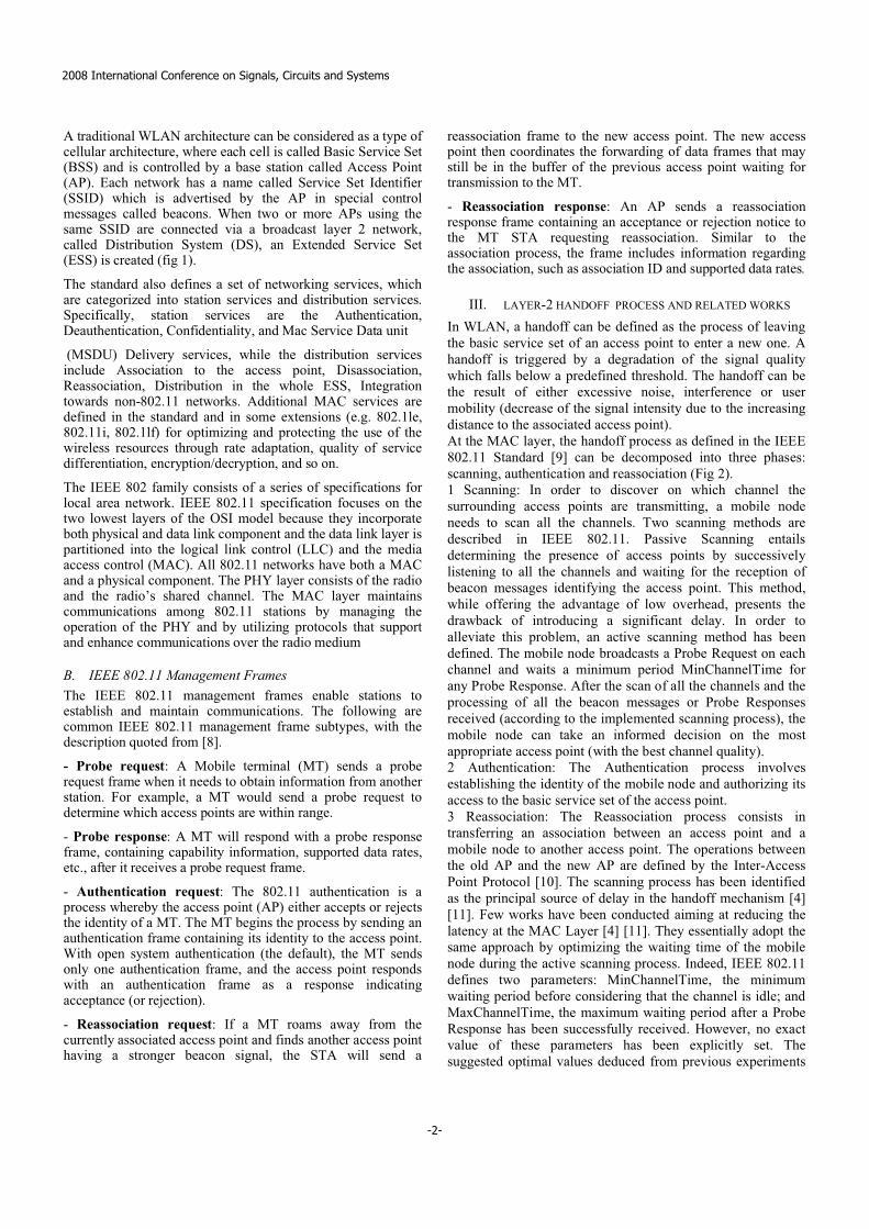
A traditional WLAN architecture can be considered as a type of cellular architecture, where each cell is called Basic Service Set (BSS) and is controlled by a base station called Access Point (AP). Each network has a name called Service Set Identifier (SSID) which is advertised by the AP in special control messages called beacons. When two or more APs using the same SSID are connected via a broadcast layer 2 network, called Distribution System (DS), an Extended Service Set (ESS) is created (fig 1).
The standard also defines a set of networking services, which are categorized into station services and distribution services. Specifically, station services are the Authentication, Deauthentication, Confidentiality, and Mac Service Data unit
(MSDU) Delivery services, while the distribution services include Association to the access point, Disassociation, Reassociation, Distribution in the whole ESS, Integration towards non-802.11 networks. Additional MAC services are defined in the standard and in some extensions (e.g. 802.1le, 802.11i, 802.1lf) for optimizing and protecting the use of the wireless resources through rate adaptation, quality of service differentiation, encryption/decryption, and so on.
The IEEE 802 family consists of a series of specifications for local area network. IEEE 802.11 specification focuses on the two lowest layers of the OSI model because they incorporate both physical and data link component and the data link layer is partitioned into the logical link control (LLC) and the media access control (MAC). All 802.11 networks have both a MAC and a physical component. The PHY layer consists of the radio and the radio’s shared channel. The MAC layer maintains communications among 802.11 stations by managing the operation of the PHY and by utilizing protocols that support and enhance communications over the radio medium
B. IEEE 802.11 Management FramesThe IEEE 802.11 management frames enable stations to establish and maintain communications. The following are common IEEE 802.11 management frame subtypes, with the description quoted from [8].
- Probe request: A Mobile terminal (MT) sends a probe request frame when it needs to obtain information from another station. For example, a MT would send a probe request to determine which access points are within range.
- Probe response: A MT will respond with a probe response frame, containing capability information, supported data rates, etc., after it receives a probe request frame.
- Authentication request: The 802.11 authentication is a process whereby the access point (AP) either accepts or rejects the identity of a MT. The MT begins the process by sending an authentication frame containing its identity to the access point. With open system authentication (the default), the MT sends only one authentication frame, and the access point responds with an authentication frame as a response indicating acceptance (or rejection).
- Reassociation request: If a MT roams away from the currently associated access point and finds another access point having a stronger beacon signal, the STA will send a
reassociation frame to the new access point. The new access point then coordinates the forwarding of data frames that may still be in the buffer of the previous access point waiting for transmission to the MT.
- Reassociation response: An AP sends a reassociation response frame containing an acceptance or rejection notice to the MT STA requesting reassociation. Similar to the association process, the frame includes information regarding the association, such as association ID and supported data rates.
III. LAYER-2 HANDOFF PROCESS AND RELATED WORKS
In WLAN, a handoff can be defined as the process of leaving the basic service set of an access point to enter a new one. A handoff is triggered by a degradation of the signal quality which falls below a predefined threshold. The handoff can be the result of either excessive noise, interference or user mobility (decrease of the signal intensity due to the increasing distance to the associated access point).At the MAC layer, the handoff process as defined in the IEEE 802.11 Standard [9] can be decomposed into three phases: scanning, authentication and reassociation (Fig 2).1 Scanning: In order to discover on which channel the surrounding access points are transmitting, a mobile node needs to scan all the channels. Two scanning methods are described in IEEE 802.11. Passive Scanning entails determining the presence of access points by successively listening to all the channels and waiting for the reception of beacon messages identifying the access point. This method, while offering the advantage of low overhead, presents the drawback of introducing a significant delay. In order to alleviate this problem, an active scanning method has been defined. The mobile node broadcasts a Probe Request on each channel and waits a minimum period MinChannelTime for any Probe Response. After the scan of all the channels and the processing of all the beacon messages or Probe Responses received (according to the implemented scanning process), the mobile node can take an informed decision on the most appropriate access point (with the best channel quality).2 Authentication: The Authentication process involves establishing the identity of the mobile node and authorizing its access to the basic service set of the access point.3 Reassociation: The Reassociation process consists in transferring an association between an access point and a mobile node to another access point. The operations between the old AP and the new AP are defined by the Inter-Access Point Protocol [10]. The scanning process has been identified as the principal source of delay in the handoff mechanism [4][11]. Few works have been conducted aiming at reducing the latency at the MAC Layer [4] [11]. They essentially adopt the same approach by optimizing the waiting time of the mobile node during the active scanning process. Indeed, IEEE 802.11 defines two parameters: MinChannelTime, the minimum waiting period before considering that the channel is idle; and MaxChannelTime, the maximum waiting period after a Probe Response has been successfully received. However, no exact value of these parameters has been explicitly set. The suggested optimal values deduced from previous experiments
2008 International Conference on Signals, Circuits and Systems
-2-
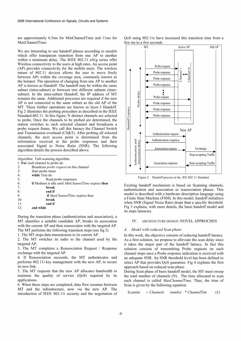
are approximately 6.5ms for MinChannelTime and 11ms for MaxChannelTime.
We are interesting to use handoff phases according to models which offer transparent transition from one AP to another within a minimum delay. The IEEE 802.11 a/b/g series offer Wireless connectivity to the users at high rates. An access point (AP) provides connectivity for the mobile users. The wireless nature of 802.11 devices allows the user to move freely between APs within the coverage area, commonly known as the hotspot. The operation of changing from one AP to another AP is known as Handoff. The handoff may be within the same subnet (intra-subnet) or between two different subnets (inter-subnet). In the intra-subnet Handoff, the IP address of MT remains the same. Additional processes are required if the new AP is not connected to the same subnet as the old AP of the MT. These further operations are known as layer-3 Handoff. Fig 2 illustrates the probing procedure as described in the IEEE Standard 802.11. In this figure, N distinct channels are selected to probe. Once the channels to be probed are determined, the station switches to each selected channel and broadcasts a probe request frame. We call this latency the Channel Switch and Transmission overhead (CS&T). After probing all selected channels, the next access point is determined from the information received in the probe responses and their associated Signal to Noise Ratio (SNR). The following algorithm details the process described above.
Algorithm: Full-scanning algorithm.1: For each channel to probe do2: Broadcast probe request on this channel3: Start probe timer4: while True do5: Read probe responses6: if Medium is idle until MinChannelTime expires then7: break8: end if9: if MaxChannelTime expires then10: break11: end if12: end while
During the transition phase (authentication and association), a MT identifies a suitable candidate AP, breaks its association with the current AP and then reassociates with the targeted AP. The MT performs the following transition steps (see fig 2)1. The MT stops data transmission to its current AP.2. The MT switches its radio to the channel used by the targeted AP.3. The MT completes a Reassociation Request / Response exchange with the targeted AP. 4. If Reassociation succeeds, the MT authenticates and performs 802.11i key management with the new AP, to secure its new link.5. The MT requests that the new AP allocates bandwidth to maintain the quality of service (QoS) required by its applications.6. When these steps are completed, data flow resumes between MT and the infrastructure, now via the new AP. The introduction of IEEE 802.11i security and the negotiation of
QoS using 802.11e have increased this transition time from a few ms to a few seconds.
MT Active AP Old AP
New AP
Probe request
Probe response
Probe response
Probe response
Probe request
Probe response
Probe response
Probe response
...
...
Cha
nnel
1
Cha
nnel
N
Authentication request
Authentication response
Association request
Association response
Exchange
Stop accepting Traffic
Start accepting Traffic
Han
doff
Lat
ency
Pro
be d
elay
Aut
hent
icat
ion
and
Ass
ocia
tion
del
ay
Figure 2. Handoff process in the IEE 802.11 Standard.
Existing handoff mechanism is based on Scanning channels, authentication and association or reassociation phases. This model is described with a hardware description language using a Finite State Machine (FSM). In this model, handoff initializes when SNR (Signal Noise Rate) drops than a specific threshold. Fig 3 explains, with more details, the basis handoff model and its steps latencies.
IV. ARCHITECTURE DESIGN: NOVEL APPROCHES
A. Model with reduced Scan phaseIn this work, the objective consists of reducing handoff latency. As a first solution, we propose to alleviate the scan delay since it takes the major part of the handoff latency. In fact this solution consists of transmitting Probe requests on each channel stops once a Probe response indication is received with an adequate SNR. An SNR threshold level has been defined to select AP that provides QoS guarantee. Fig 4 explains the first approach based on reduced scan phase.During Scan phase of basis handoff model, the MT must sweep the total number of channels (N). The time allocated to scan each channel is called MaxChannelTime. Thus, the time of Scan is given by the following equation.
)1(* ChannelTimnumberChannelsScantim �
2008 International Conference on Signals, Circuits and Systems
-3-
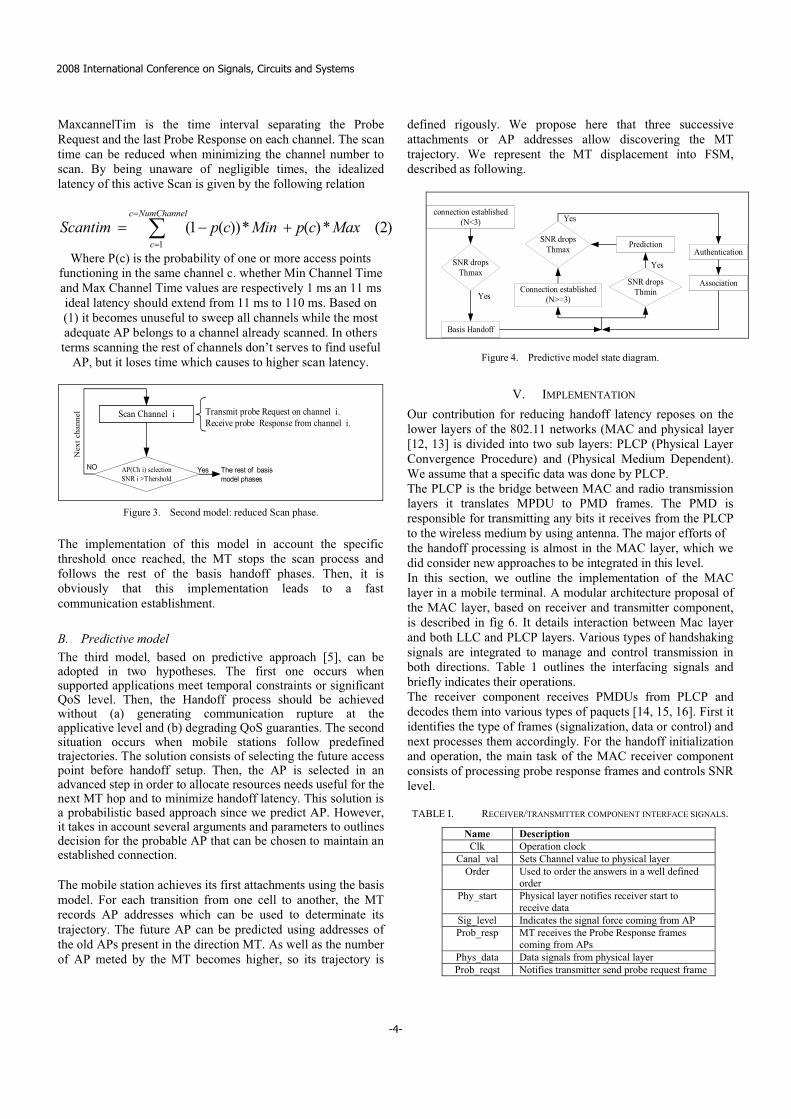
MaxcannelTim is the time interval separating the Probe Request and the last Probe Response on each channel. The scan time can be reduced when minimizing the channel number to scan. By being unaware of negligible times, the idealized latency of this active Scan is given by the following relation
)2(*)(*))(1(1�
�
�
���NumChannelc
cMaxcpMincpScantim
Where P(c) is the probability of one or more access points functioning in the same channel c. whether Min Channel Time and Max Channel Time values are respectively 1 ms an 11 ms ideal latency should extend from 11 ms to 110 ms. Based on (1) it becomes unuseful to sweep all channels while the most adequate AP belongs to a channel already scanned. In others terms scanning the rest of channels don’t serves to find useful
AP, but it loses time which causes to higher scan latency.
Scan Channel i
AP(Ch i) selectionSNR i >Thershold
The rest of basismodel phases
Nex
t cha
nnel Transmit probe Request on channel i.
Receive probe Response from channel i.
YesNO
Figure 3. Second model: reduced Scan phase.
The implementation of this model in account the specific threshold once reached, the MT stops the scan process and follows the rest of the basis handoff phases. Then, it is obviously that this implementation leads to a fast communication establishment.
B. Predictive modelThe third model, based on predictive approach [5], can be adopted in two hypotheses. The first one occurs when supported applications meet temporal constraints or significant QoS level. Then, the Handoff process should be achieved without (a) generating communication rupture at the applicative level and (b) degrading QoS guaranties. The second situation occurs when mobile stations follow predefined trajectories. The solution consists of selecting the future access point before handoff setup. Then, the AP is selected in an advanced step in order to allocate resources needs useful for the next MT hop and to minimize handoff latency. This solution is a probabilistic based approach since we predict AP. However, it takes in account several arguments and parameters to outlines decision for the probable AP that can be chosen to maintain an established connection.
The mobile station achieves its first attachments using the basis model. For each transition from one cell to another, the MT records AP addresses which can be used to determinate its trajectory. The future AP can be predicted using addresses of the old APs present in the direction MT. As well as the number of AP meted by the MT becomes higher, so its trajectory is
defined rigously. We propose here that three successive attachments or AP addresses allow discovering the MT trajectory. We represent the MT displacement into FSM, described as following.
connection established(N<3)
SNR dropsThmax
Basis Handoff
Connection established(N>=3)
SNR dropsThmin
PredictionSNR dropsThmax Authentication
Association
Yes
Yes
Yes
Figure 4. Predictive model state diagram.
V. IMPLEMENTATION
Our contribution for reducing handoff latency reposes on the lower layers of the 802.11 networks (MAC and physical layer [12, 13] is divided into two sub layers: PLCP (Physical Layer Convergence Procedure) and (Physical Medium Dependent). We assume that a specific data was done by PLCP.The PLCP is the bridge between MAC and radio transmission layers it translates MPDU to PMD frames. The PMD is responsible for transmitting any bits it receives from the PLCP to the wireless medium by using antenna. The major efforts of the handoff processing is almost in the MAC layer, which we did consider new approaches to be integrated in this level. In this section, we outline the implementation of the MAC layer in a mobile terminal. A modular architecture proposal of the MAC layer, based on receiver and transmitter component, is described in fig 6. It details interaction between Mac layer and both LLC and PLCP layers. Various types of handshaking signals are integrated to manage and control transmission in both directions. Table 1 outlines the interfacing signals and briefly indicates their operations.The receiver component receives PMDUs from PLCP and decodes them into various types of paquets [14, 15, 16]. First it identifies the type of frames (signalization, data or control) and next processes them accordingly. For the handoff initialization and operation, the main task of the MAC receiver component consists of processing probe response frames and controls SNR level.
TABLE I. RECEIVER/TRANSMITTER COMPONENT INTERFACE SIGNALS.
Name DescriptionClk Operation clock
Canal_val Sets Channel value to physical layerOrder Used to order the answers in a well defined
orderPhy_start Physical layer notifies receiver start to
receive dataSig_level Indicates the signal force coming from APProb_resp MT receives the Probe Response frames
coming from APsPhys_data Data signals from physical layerProb_reqst Notifies transmitter send probe request frame
2008 International Conference on Signals, Circuits and Systems
-4-
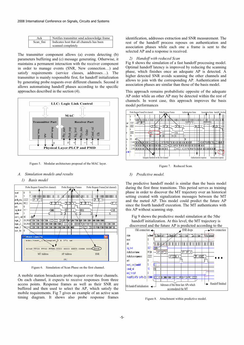
Ack Notifies transmitter send acknowledge frameScan_fini Indicates host that all channels has been
scanned completely
The transmitter component allows (a) events detecting (b) parameters buffering and (c) message generating. Otherwise, it maintains a permanent interaction with the receiver component in order to manage events (SNR, New connection…) and satisfy requirements (service classes, addresses…). The transmitter is mainly responsible first, for handoff initialization by generating probe requests over different channels. Second it allows automatising handoff phases according to the specific approaches described in the section (4).
Phy_
start
Prob
_resp
Sig_le
vel
Phys_
dataProb_reqst
Ack Ca
nal_v
al
Orde
rScan_fini
Physical Layer:PLCP and PMD
MAC
LLC: Logic Link Control
Clk
Transmitter Part Receiver Part
16 4 2 416
Figure 5. Modular architecture proposal of the MAC layer.
A. Simulation models and results1) Basis model
Probe Response FramesProbe Request Frame(First channel)
MT Address AP Address SNR
Probe Request Frame(2nd channel)
Figure 6. Simulation of Scan Phase on the first channel.
A mobile station broadcasts probe request over three channels. On each channel, it expects to receive responses from three access points. Response frames as well as their SNR are buffered and then used to select the AP, which satisfy the mobile requirements. Fig 7 gives an example of an active scan timing diagram. It shows also probe response frames
identification, addresses extraction and SNR measurement. The rest of the handoff process reposes on authentication and association phases while each one a frame is sent to the selected AP and a response is received.
2) Handoff with reduced ScanFig 8 shows the simulation of a fast handoff processing model. Optimal handoff latency is improved by reducing the scanning phase, which finishes once an adequate AP is detected. A higher detected SNR avoids scanning the other channels and allows to join with the corresponding AP. Authentication and association phases are similar than those of the basis model.
This approach remains probabilistic opposite of the adequate AP order while an other AP may be detected within the rest of channels. In worst case, this approach improves the basis model performances
Probe Request Frame(First channel) Probe Response Frames Authentication frame Association frame
Association responseAdequate thershold on the first channel Authentication response
handoff finished
Figure 7. Reduced Scan.
3) Predictive model.
The predictive handoff model is similar than the basis model during the first three transitions. This period serves as training phase in order to discover the MT trajectory over an historical setting created with signalization messages between the MT and the meted AP. This model could predict the future AP since the fourth handoff execution. The MT authenticates with this AP without scanning step.
Fig 9 shows the predictive model simulation at the 5the handoff initialization. At this level, the MT trajectory is
discovered and the future AP is predicted according to the SNR drops
5th handoff initialisation Adresses of the three last APs whichaccomodated the MT
Old connection New connection
Handoff finished
...
Figure 8. Attachment within predictive model.
2008 International Conference on Signals, Circuits and Systems
-5-
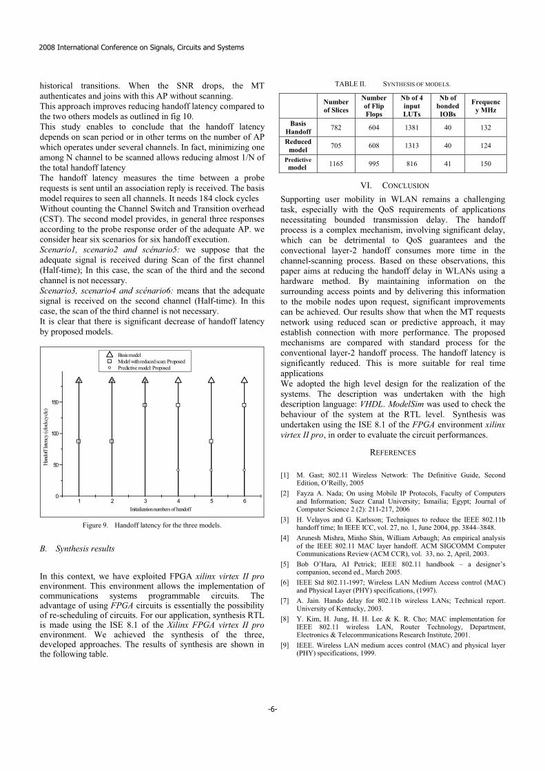
historical transitions. When the SNR drops, the MT authenticates and joins with this AP without scanning.This approach improves reducing handoff latency compared to the two others models as outlined in fig 10.This study enables to conclude that the handoff latency depends on scan period or in other terms on the number of AP which operates under several channels. In fact, minimizing one among N channel to be scanned allows reducing almost 1/N of the total handoff latencyThe handoff latency measures the time between a probe requests is sent until an association reply is received. The basis model requires to seen all channels. It needs 184 clock cycles Without counting the Channel Switch and Transition overhead (CST). The second model provides, in general three responses according to the probe response order of the adequate AP. we consider hear six scenarios for six handoff execution.Scenario1, scenario2 and scénario5: we suppose that the adequate signal is received during Scan of the first channel (Half-time); In this case, the scan of the third and the secondchannel is not necessary.Scenario3, scenario4 and scénario6: means that the adequate signal is received on the second channel (Half-time). In this case, the scan of the third channel is not necessary.It is clear that there is significant decrease of handoff latency by proposed models.
1 2 3 4 5 60
50
100
150
Hand
off l
atenc
y (c
lock c
ycle)
Initialization numbers of handoff
Basis model Model with reduced scan: Proposed Predictive model: Proposed
Figure 9. Handoff latency for the three models.
B. Synthesis results
In this context, we have exploited FPGA xilinx virtex II proenvironment. This environment allows the implementation of communications systems programmable circuits. The advantage of using FPGA circuits is essentially the possibility of re-scheduling of circuits. For our application, synthesis RTL is made using the ISE 8.1 of the Xilinx FPGA virtex II proenvironment. We achieved the synthesis of the three, developed approaches. The results of synthesis are shown in the following table.
TABLE II. SYNTHESIS OF MODELS.
Number of Slices
Number of Flip Flops
Nb of 4 input LUTs
Nb of bonded IOBs
Frequency MHz
Basis Handoff 782 604 1381 40 132
Reduced model 705 608 1313 40 124
Predictive model 1165 995 816 41 150
VI. CONCLUSION
Supporting user mobility in WLAN remains a challenging task, especially with the QoS requirements of applications necessitating bounded transmission delay. The handoff process is a complex mechanism, involving significant delay, which can be detrimental to QoS guarantees and theconvectional layer-2 handoff consumes more time in the channel-scanning process. Based on these observations, this paper aims at reducing the handoff delay in WLANs using a hardware method. By maintaining information on the surrounding access points and by delivering this information to the mobile nodes upon request, significant improvements can be achieved. Our results show that when the MT requests network using reduced scan or predictive approach, it may establish connection with more performance. The proposed mechanisms are compared with standard process for the conventional layer-2 handoff process. The handoff latency is significantly reduced. This is more suitable for real time applicationsWe adopted the high level design for the realization of the systems. The description was undertaken with the high description language: VHDL. ModelSim was used to check the behaviour of the system at the RTL level. Synthesis was undertaken using the ISE 8.1 of the FPGA environment xilinx virtex II pro, in order to evaluate the circuit performances.
REFERENCES
[1] M. Gast; 802.11 Wireless Network: The Definitive Guide, Second Edition, O’Reilly, 2005
[2] Fayza A. Nada; On using Mobile IP Protocols, Faculty of Computers and Information; Suez Canal University; Ismailia; Egypt; Journal of Computer Science 2 (2): 211-217, 2006
[3] H. Velayos and G. Karlsson; Techniques to reduce the IEEE 802.11b handoff time; In IEEE ICC, vol. 27, no. 1, June 2004, pp. 3844–3848.
[4] Arunesh Mishra, Minho Shin, William Arbaugh; An empirical analysis of the IEEE 802.11 MAC layer handoff. ACM SIGCOMM Computer Communications Review (ACM CCR), vol. 33, no. 2, April, 2003.
[5] Bob O’Hara, AI Petrick; IEEE 802.11 handbook – a designer’s companion, second ed., March 2005.
[6] IEEE Std 802.11-1997; Wireless LAN Medium Access control (MAC) and Physical Layer (PHY) specifications, (1997).
[7] A. Jain. Hando delay for 802.11b wireless LANs; Technical report. University of Kentucky, 2003.
[8] Y. Kim, H. Jung, H. H. Lee & K. R. Cho; MAC implementation for IEEE 802.11 wireless LAN, Router Technology, Department, Electronics & Telecommunications Research Institute, 2001.
[9] IEEE. Wireless LAN medium acces control (MAC) and physical layer (PHY) specifications, 1999.
2008 International Conference on Signals, Circuits and Systems
-6-
[10] IEEE. IEEE trial-use recommended practice for multi-vendor acces point interoperability via an inter acces point protocol across distribution systems supporting IEEE 802.11 operation, 2003.
[11] H. Velayos and karlsson G. Technique to reduce the IEEE 802.11b handoff time. In swedish National computer networking Workshop,2003
[12] IEEE 802.11, IEEE wireless LAN medium access control (MAC) and physical layer (PHY) specifications, Aug. 1999
[13] IEEE 802.11b, Wireless LAN medium access control (MAC) and physical layer (PHY) specifications: High-speed Physical Layer Extension in the 2.4GHz Band, IEEE Std 802.11b-1999
[14] Y. Kim, H. Jung, H. H. Lee & K. R. Cho, MAC implementation for IEEE 802.11 wireless LAN, Router Technology, Department,Electronics & Telecommunications Research Institute, 2001.
[15] XILINX, configurable Locallink CRC Reference Design, Nov, 2004[16] T. H. Meng; Design and implementation of an all-CMOS 802.11a
wireless LAN chipset, Communication magazine, IEEE, Vol.41, No.8, Aug. 2003.
SETIT 2004 International Conference: Sciences of Electronic,
Technologies of Information and Telecommunications March 15-20, 2004 – TUNISIA
Interopérabilité ETHERNET/WATM
Jamila BHAR; Ridha OUNI; Salem NASRI
Laboratoire d’Electronique et de Micro-Electronique (EµE), Faculté des Sciences de Monastir, Tunisie
Résumé— Parmi les besoins actuels dans le domaine de télécommunication, Nous distinguons le recourt à l’implantation des applications multimédias sur diverses architectures. Dans cet environnement hétérogène, une multitude de normes s’interfère interdisant l’interconnexion directe des réseaux. La complexité de l’interconnexion dépend de l’incompatibilité protocolaire des réseaux définis par la dissymétrie à chaque niveau de leurs modèles en couches. D’ailleurs, les passerelles sont les systèmes les plus complexes permettant l’interconnexion des réseaux. Cet article se dirige dans le cadre de l’interopérabilité des réseaux hétérogènes. La contribution principale de ce travail est le développement d’un mécanisme de conversion d’informations pouvant être échangées lors de l’interopérabilité Ethernet/WATM. L’interface proposée se charge de la gestion des procédures liées à la segmentation et au réassemblage des données.
La démarche suivie consiste en première étape à l’étude et à la spécification de l’interconnexion Ethernet/WATM. La deuxième étape a pour but de définir le flot de conception et la description des fonctions d’interconnexions. Dans la dernière étape, nous présentons les résultats acquis et nous mentionnons la possibilité d’entrevoir des nouveaux horizons pour optimiser l’approche proposée. Afin d’implémenter les fonctions élémentaires d’interconnexion, nous avons utilisé le langage de description VHDL et les outils de simulation et de synthèse V_system et FPGA_Adv.
Mots Clés: — Réseau, Interconnexion, Ethernet, WATM, VHDL.
1 INTRODUCTION La diversité des réseaux, l’orientation vers les
réseaux sans fils et le besoin de l’intégration des applications sur des architectures hétérogènes ont favorisé la tendance de la conception des systèmes d’interconnexion. Ces derniers permettent de fournir une large gamme de services multimédias et visent à homogénéiser l’environnement de communication.
Les tendances des recherches actuelles dans le domaine des réseaux s’orientent à l’exploitation de la diversité des réseaux. Ceci permet de profiter des avantages offerts par chacun et de développer des applications basées sur diverses architectures. L’étude et la contribution à l’interopérabilité des réseaux répandus avec ceux sans fils sont fortement demandées. Dans ce contexte, l’interfonctionnement Ethernet/WATM donne un exemple concret compte
tenu des caractéristiques et des performances de deux infrastructures.
Lors de l’interopérabilité entre les deux réseaux, de nombreux problèmes sont posés par l’hétérogénéité de l’environnement de communication. Les données transitant entre les deux réseaux utilisent des formats incompatibles. Les débits et les mécanismes de transmissions ainsi que les politiques de connexion sont propres à chaque réseau. Ce travail est une contribution à la conception d’un système d’interconnexion Ethernet/WATM. Nous nous intéressons à la spécification de l’interface cible ainsi que la conception d’un mécanisme de conversion de format de l’information.
Dans cet article, nous introduisons l’environnement de l’application. Puis, nous présentons les systèmes d’interfaçage entre réseaux hétérogènes. Nous décrivons, ensuite, le flot de
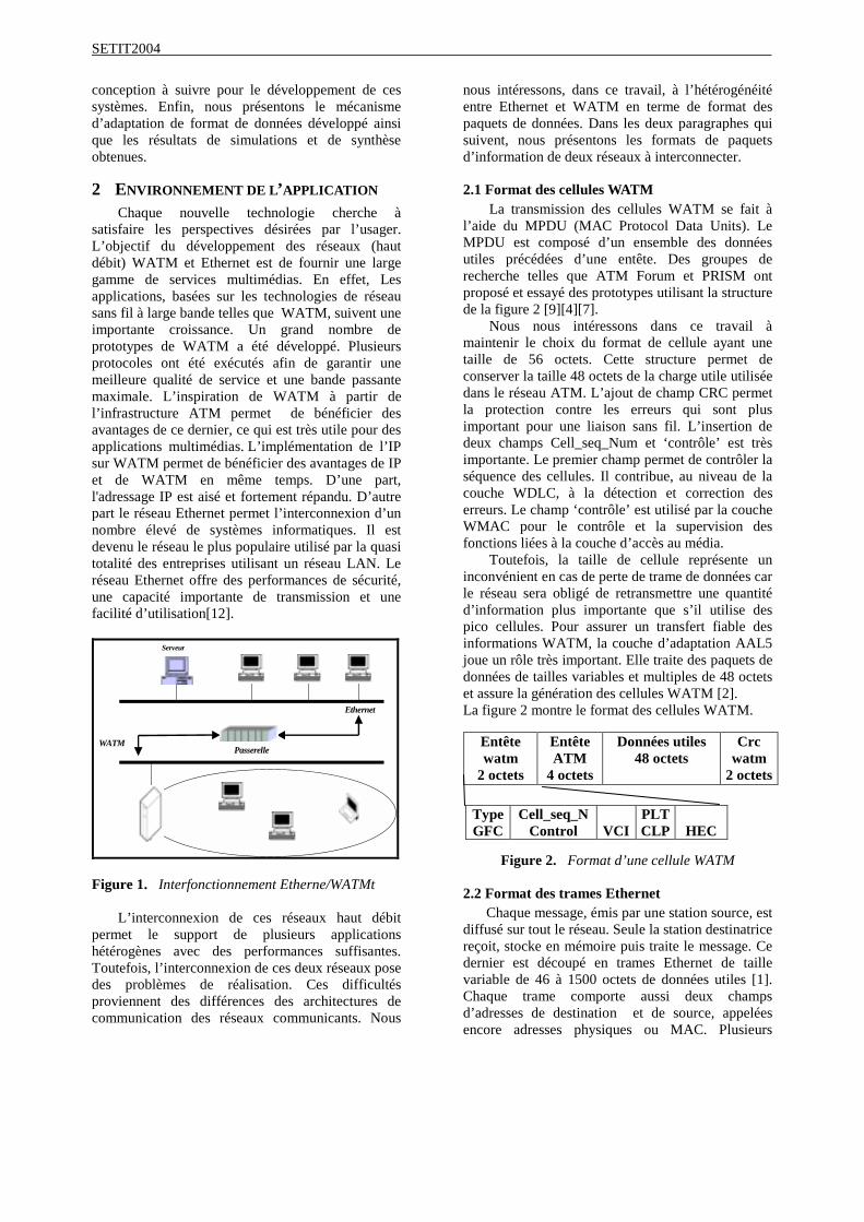
SETIT2004
conception à suivre pour le développement de ces systèmes. Enfin, nous présentons le mécanisme d’adaptation de format de données développé ainsi que les résultats de simulations et de synthèse obtenues.
2 ENVIRONNEMENT DE L’APPLICATION Chaque nouvelle technologie cherche à
satisfaire les perspectives désirées par l’usager. L’objectif du développement des réseaux (haut débit) WATM et Ethernet est de fournir une large gamme de services multimédias. En effet, Les applications, basées sur les technologies de réseau sans fil à large bande telles que WATM, suivent une importante croissance. Un grand nombre de prototypes de WATM a été développé. Plusieurs protocoles ont été exécutés afin de garantir une meilleure qualité de service et une bande passante maximale. L’inspiration de WATM à partir de l’infrastructure ATM permet de bénéficier des avantages de ce dernier, ce qui est très utile pour des applications multimédias. L’implémentation de l’IP sur WATM permet de bénéficier des avantages de IP et de WATM en même temps. D’une part, l'adressage IP est aisé et fortement répandu. D’autre part le réseau Ethernet permet l’interconnexion d’un nombre élevé de systèmes informatiques. Il est devenu le réseau le plus populaire utilisé par la quasi totalité des entreprises utilisant un réseau LAN. Le réseau Ethernet offre des performances de sécurité, une capacité importante de transmission et une facilité d’utilisation[12].
Ethernet
Serveur
Passerelle WATM
Figure 1. Interfonctionnement Etherne/WATMt
L’interconnexion de ces réseaux haut débit permet le support de plusieurs applications hétérogènes avec des performances suffisantes. Toutefois, l’interconnexion de ces deux réseaux pose des problèmes de réalisation. Ces difficultés proviennent des différences des architectures de communication des réseaux communicants. Nous
nous intéressons, dans ce travail, à l’hétérogénéité entre Ethernet et WATM en terme de format des paquets de données. Dans les deux paragraphes qui suivent, nous présentons les formats de paquets d’information de deux réseaux à interconnecter.
2.1 Format des cellules WATM
La transmission des cellules WATM se fait à l’aide du MPDU (MAC Protocol Data Units). Le MPDU est composé d’un ensemble des données utiles précédées d’une entête. Des groupes de recherche telles que ATM Forum et PRISM ont proposé et essayé des prototypes utilisant la structure de la figure 2 [9][4][7].
Nous nous intéressons dans ce travail à maintenir le choix du format de cellule ayant une taille de 56 octets. Cette structure permet de conserver la taille 48 octets de la charge utile utilisée dans le réseau ATM. L’ajout de champ CRC permet la protection contre les erreurs qui sont plus important pour une liaison sans fil. L’insertion de deux champs Cell_seq_Num et ‘contrôle’ est très importante. Le premier champ permet de contrôler la séquence des cellules. Il contribue, au niveau de la couche WDLC, à la détection et correction des erreurs. Le champ ‘contrôle’ est utilisé par la couche WMAC pour le contrôle et la supervision des fonctions liées à la couche d’accès au média.
Toutefois, la taille de cellule représente un inconvénient en cas de perte de trame de données car le réseau sera obligé de retransmettre une quantité d’information plus importante que s’il utilise des pico cellules. Pour assurer un transfert fiable des informations WATM, la couche d’adaptation AAL5 joue un rôle très important. Elle traite des paquets de données de tailles variables et multiples de 48 octets et assure la génération des cellules WATM [2]. La figure 2 montre le format des cellules WATM.
Figure 2. Format d’une cellule WATM
2.2 Format des trames Ethernet Chaque message, émis par une station source, est
diffusé sur tout le réseau. Seule la station destinatrice reçoit, stocke en mémoire puis traite le message. Ce dernier est découpé en trames Ethernet de taille variable de 46 à 1500 octets de données utiles [1]. Chaque trame comporte aussi deux champs d’adresses de destination et de source, appelées encore adresses physiques ou MAC. Plusieurs
Entête watm
2 octets
Entête ATM
4 octets
Données utiles 48 octets
Crc watm
2 octets
TypeGFC
Cell_seq_NControl
VCI
PLT CLP
HEC
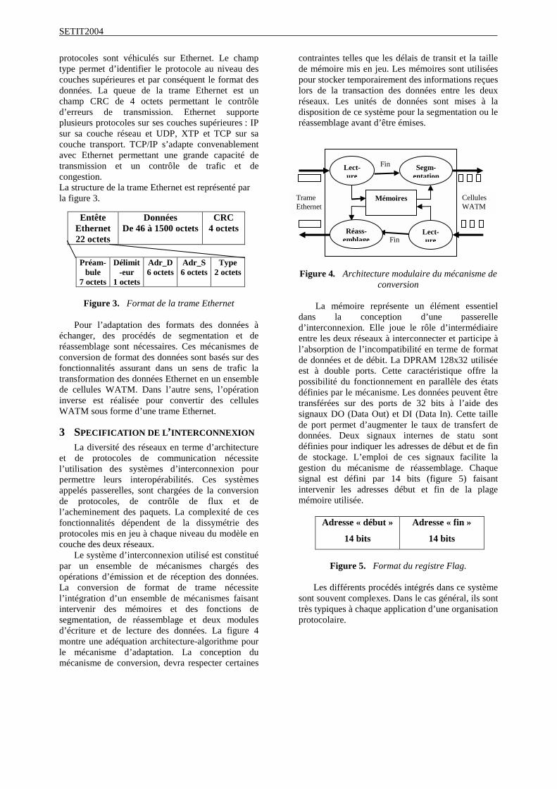
SETIT2004
protocoles sont véhiculés sur Ethernet. Le champ type permet d’identifier le protocole au niveau des couches supérieures et par conséquent le format des données. La queue de la trame Ethernet est un champ CRC de 4 octets permettant le contrôle d’erreurs de transmission. Ethernet supporte plusieurs protocoles sur ses couches supérieures : IP sur sa couche réseau et UDP, XTP et TCP sur sa couche transport. TCP/IP s’adapte convenablement avec Ethernet permettant une grande capacité de transmission et un contrôle de trafic et de congestion. La structure de la trame Ethernet est représenté par la figure 3.
Figure 3. Format de la trame Ethernet
Pour l’adaptation des formats des données à
échanger, des procédés de segmentation et de réassemblage sont nécessaires. Ces mécanismes de conversion de format des données sont basés sur des fonctionnalités assurant dans un sens de trafic la transformation des données Ethernet en un ensemble de cellules WATM. Dans l’autre sens, l’opération inverse est réalisée pour convertir des cellules WATM sous forme d’une trame Ethernet.
3 SPECIFICATION DE L’INTERCONNEXION La diversité des réseaux en terme d’architecture
et de protocoles de communication nécessite l’utilisation des systèmes d’interconnexion pour permettre leurs interopérabilités. Ces systèmes appelés passerelles, sont chargées de la conversion de protocoles, de contrôle de flux et de l’acheminement des paquets. La complexité de ces fonctionnalités dépendent de la dissymétrie des protocoles mis en jeu à chaque niveau du modèle en couche des deux réseaux.
Le système d’interconnexion utilisé est constitué par un ensemble de mécanismes chargés des opérations d’émission et de réception des données. La conversion de format de trame nécessite l’intégration d’un ensemble de mécanismes faisant intervenir des mémoires et des fonctions de segmentation, de réassemblage et deux modules d’écriture et de lecture des données. La figure 4 montre une adéquation architecture-algorithme pour le mécanisme d’adaptation. La conception du mécanisme de conversion, devra respecter certaines
contraintes telles que les délais de transit et la taille de mémoire mis en jeu. Les mémoires sont utilisées pour stocker temporairement des informations reçues lors de la transaction des données entre les deux réseaux. Les unités de données sont mises à la disposition de ce système pour la segmentation ou le réassemblage avant d’être émises.
Figure 4. Architecture modulaire du mécanisme de conversion
La mémoire représente un élément essentiel
dans la conception d’une passerelle d’interconnexion. Elle joue le rôle d’intermédiaire entre les deux réseaux à interconnecter et participe à l’absorption de l’incompatibilité en terme de format de données et de débit. La DPRAM 128x32 utilisée est à double ports. Cette caractéristique offre la possibilité du fonctionnement en parallèle des états définies par le mécanisme. Les données peuvent être transférées sur des ports de 32 bits à l’aide des signaux DO (Data Out) et DI (Data In). Cette taille de port permet d’augmenter le taux de transfert de données. Deux signaux internes de statu sont définies pour indiquer les adresses de début et de fin de stockage. L’emploi de ces signaux facilite la gestion du mécanisme de réassemblage. Chaque signal est défini par 14 bits (figure 5) faisant intervenir les adresses début et fin de la plage mémoire utilisée.
Adresse « début »
14 bits
Adresse « fin »
14 bits
Figure 5. Format du registre Flag.
Les différents procédés intégrés dans ce système sont souvent complexes. Dans le cas général, ils sont très typiques à chaque application d’une organisation protocolaire.
Entête Ethernet 22 octets
Données De 46 à 1500 octets
CRC 4 octets
Préam-bule
7 octets
Délimit-eur
1 octets
Adr_D6 octets
Adr_S 6 octets
Type 2 octets
Trame Ethernet
Cellules WATM
Fin
Fin
Lect-ure
Segm-entation
Mémoires
Lect-ure
Réass-emblage
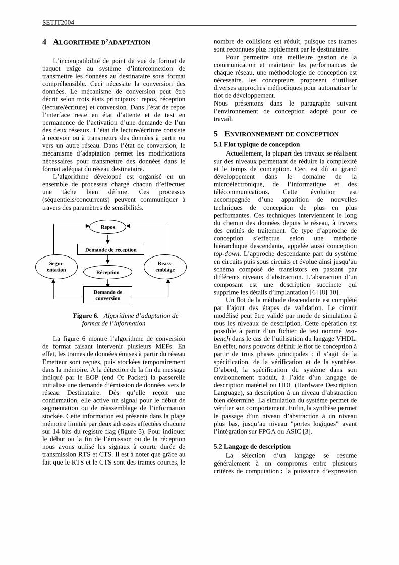
SETIT2004
4 ALGORITHME D’ADAPTATION
L’incompatibilité de point de vue de format de paquet exige au système d’interconnexion de transmettre les données au destinataire sous format compréhensible. Ceci nécessite la conversion des données. Le mécanisme de conversion peut être décrit selon trois états principaux : repos, réception (lecture/écriture) et conversion. Dans l’état de repos l’interface reste en état d’attente et de test en permanence de l’activation d’une demande de l’un des deux réseaux. L’état de lecture/écriture consiste à recevoir ou à transmettre des données à partir ou vers un autre réseau. Dans l’état de conversion, le mécanisme d’adaptation permet les modifications nécessaires pour transmettre des données dans le format adéquat du réseau destinataire.
L’algorithme développé est organisé en un ensemble de processus chargé chacun d’effectuer une tâche bien définie. Ces processus (séquentiels/concurrents) peuvent communiquer à travers des paramètres de sensibilités.
Figure 6. Algorithme d’adaptation de format de l’information
La figure 6 montre l’algorithme de conversion
de format faisant intervenir plusieurs MEFs. En effet, les trames de données émises à partir du réseau Emetteur sont reçues, puis stockées temporairement dans la mémoire. A la détection de la fin du message indiqué par le EOP (end Of Packet) la passerelle initialise une demande d’émission de données vers le réseau Destinataire. Dès qu’elle reçoit une confirmation, elle active un signal pour le début de segmentation ou de réassemblage de l’information stockée. Cette information est présente dans la plage mémoire limitée par deux adresses affectées chacune sur 14 bits du registre flag (figure 5). Pour indiquer le début ou la fin de l’émission ou de la réception nous avons utilisé les signaux à courte durée de transmission RTS et CTS. Il est à noter que grâce au fait que le RTS et le CTS sont des trames courtes, le
nombre de collisions est réduit, puisque ces trames sont reconnues plus rapidement par le destinataire.
Pour permettre une meilleure gestion de la communication et maintenir les performances de chaque réseau, une méthodologie de conception est nécessaire. les concepteurs proposent d’utiliser diverses approches méthodiques pour automatiser le flot de développement. Nous présentons dans le paragraphe suivant l’environnement de conception adopté pour ce travail.
5 ENVIRONNEMENT DE CONCEPTION 5.1 Flot typique de conception
Actuellement, la plupart des travaux se réalisent sur des niveaux permettant de réduire la complexité et le temps de conception. Ceci est dû au grand développement dans le domaine de la microélectronique, de l’informatique et des télécommunications. Cette évolution est accompagnée d’une apparition de nouvelles techniques de conception de plus en plus performantes. Ces techniques interviennent le long du chemin des données depuis le réseau, à travers des entités de traitement. Ce type d’approche de conception s’effectue selon une méthode hiérarchique descendante, appelée aussi conception top-down. L’approche descendante part du système en circuits puis sous circuits et évolue ainsi jusqu’au schéma composé de transistors en passant par différents niveaux d’abstraction. L’abstraction d’un composant est une description succincte qui supprime les détails d’implantation [6] [8][10].
Un flot de la méthode descendante est complété par l’ajout des étapes de validation. Le circuit modélisé peut être validé par mode de simulation à tous les niveaux de description. Cette opération est possible à partir d’un fichier de test nommé test-bench dans le cas de l’utilisation du langage VHDL. En effet, nous pouvons définir le flot de conception à partir de trois phases principales : il s’agit de la spécification, de la vérification et de la synthèse. D’abord, la spécification du système dans son environnement traduit, à l’aide d’un langage de description matériel ou HDL (Hardware Description Language), sa description à un niveau d’abstraction bien déterminé. La simulation du système permet de vérifier son comportement. Enfin, la synthèse permet le passage d’un niveau d’abstraction à un niveau plus bas, jusqu’au niveau "portes logiques" avant l’intégration sur FPGA ou ASIC [3]. 5.2 Langage de description
La sélection d’un langage se résume généralement à un compromis entre plusieurs critères de computation : la puissance d’expression
Repos
Demande de réception
Réception
Demande de conversion
Reass-emblage
Segm-entation
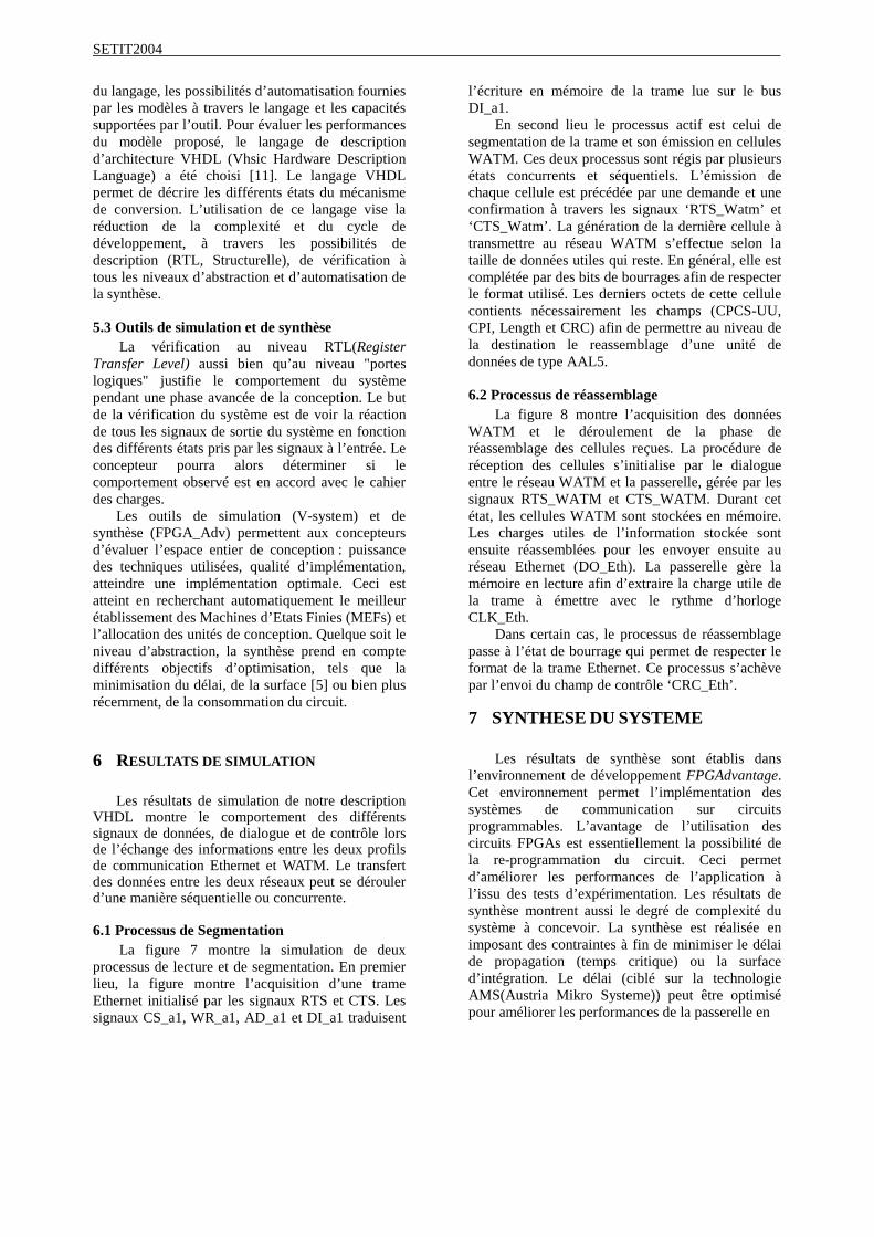
SETIT2004
du langage, les possibilités d’automatisation fournies par les modèles à travers le langage et les capacités supportées par l’outil. Pour évaluer les performances du modèle proposé, le langage de description d’architecture VHDL (Vhsic Hardware Description Language) a été choisi [11]. Le langage VHDL permet de décrire les différents états du mécanisme de conversion. L’utilisation de ce langage vise la réduction de la complexité et du cycle de développement, à travers les possibilités de description (RTL, Structurelle), de vérification à tous les niveaux d’abstraction et d’automatisation de la synthèse. 5.3 Outils de simulation et de synthèse
La vérification au niveau RTL(Register Transfer Level) aussi bien qu’au niveau "portes logiques" justifie le comportement du système pendant une phase avancée de la conception. Le but de la vérification du système est de voir la réaction de tous les signaux de sortie du système en fonction des différents états pris par les signaux à l’entrée. Le concepteur pourra alors déterminer si le comportement observé est en accord avec le cahier des charges.
Les outils de simulation (V-system) et de synthèse (FPGA_Adv) permettent aux concepteurs d’évaluer l’espace entier de conception : puissance des techniques utilisées, qualité d’implémentation, atteindre une implémentation optimale. Ceci est atteint en recherchant automatiquement le meilleur établissement des Machines d’Etats Finies (MEFs) et l’allocation des unités de conception. Quelque soit le niveau d’abstraction, la synthèse prend en compte différents objectifs d’optimisation, tels que la minimisation du délai, de la surface [5] ou bien plus récemment, de la consommation du circuit.
6 RESULTATS DE SIMULATION
Les résultats de simulation de notre description VHDL montre le comportement des différents signaux de données, de dialogue et de contrôle lors de l’échange des informations entre les deux profils de communication Ethernet et WATM. Le transfert des données entre les deux réseaux peut se dérouler d’une manière séquentielle ou concurrente. 6.1 Processus de Segmentation
La figure 7 montre la simulation de deux processus de lecture et de segmentation. En premier lieu, la figure montre l’acquisition d’une trame Ethernet initialisé par les signaux RTS et CTS. Les signaux CS_a1, WR_a1, AD_a1 et DI_a1 traduisent
l’écriture en mémoire de la trame lue sur le bus DI_a1.
En second lieu le processus actif est celui de segmentation de la trame et son émission en cellules WATM. Ces deux processus sont régis par plusieurs états concurrents et séquentiels. L’émission de chaque cellule est précédée par une demande et une confirmation à travers les signaux ‘RTS_Watm’ et ‘CTS_Watm’. La génération de la dernière cellule à transmettre au réseau WATM s’effectue selon la taille de données utiles qui reste. En général, elle est complétée par des bits de bourrages afin de respecter le format utilisé. Les derniers octets de cette cellule contients nécessairement les champs (CPCS-UU, CPI, Length et CRC) afin de permettre au niveau de la destination le reassemblage d’une unité de données de type AAL5. 6.2 Processus de réassemblage
La figure 8 montre l’acquisition des données WATM et le déroulement de la phase de réassemblage des cellules reçues. La procédure de réception des cellules s’initialise par le dialogue entre le réseau WATM et la passerelle, gérée par les signaux RTS_WATM et CTS_WATM. Durant cet état, les cellules WATM sont stockées en mémoire. Les charges utiles de l’information stockée sont ensuite réassemblées pour les envoyer ensuite au réseau Ethernet (DO_Eth). La passerelle gère la mémoire en lecture afin d’extraire la charge utile de la trame à émettre avec le rythme d’horloge CLK_Eth.
Dans certain cas, le processus de réassemblage passe à l’état de bourrage qui permet de respecter le format de la trame Ethernet. Ce processus s’achève par l’envoi du champ de contrôle ‘CRC_Eth’.
7 SYNTHESE DU SYSTEME
Les résultats de synthèse sont établis dans l’environnement de développement FPGAdvantage. Cet environnement permet l’implémentation des systèmes de communication sur circuits programmables. L’avantage de l’utilisation des circuits FPGAs est essentiellement la possibilité de la re-programmation du circuit. Ceci permet d’améliorer les performances de l’application à l’issu des tests d’expérimentation. Les résultats de synthèse montrent aussi le degré de complexité du système à concevoir. La synthèse est réalisée en imposant des contraintes à fin de minimiser le délai de propagation (temps critique) ou la surface d’intégration. Le délai (ciblé sur la technologie AMS(Austria Mikro Systeme)) peut être optimisé pour améliorer les performances de la passerelle en
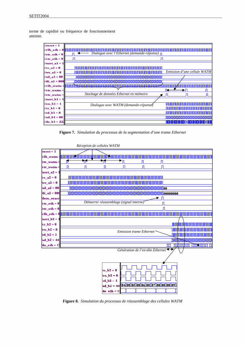
SETIT2004
terme de rapidité ou fréquence de fonctionnement atteinte.
Figure 7. Simulation du processus de la segmentation d’une trame Ethernet
Figure 8. Simulation du processus de réassemblage des cellules WATM
Réception de cellules WATM
Démarrer réassemblage (signal interne)
Génération de l’en-tête Ethernet
Emission trame Ethernet
Stockage de données Ethernet en mémoire
Emission d’une cellule WATM
Dialogue avec l’Ethernet (demande-réponse)
Dialogue avec WATM (demande-réponse)
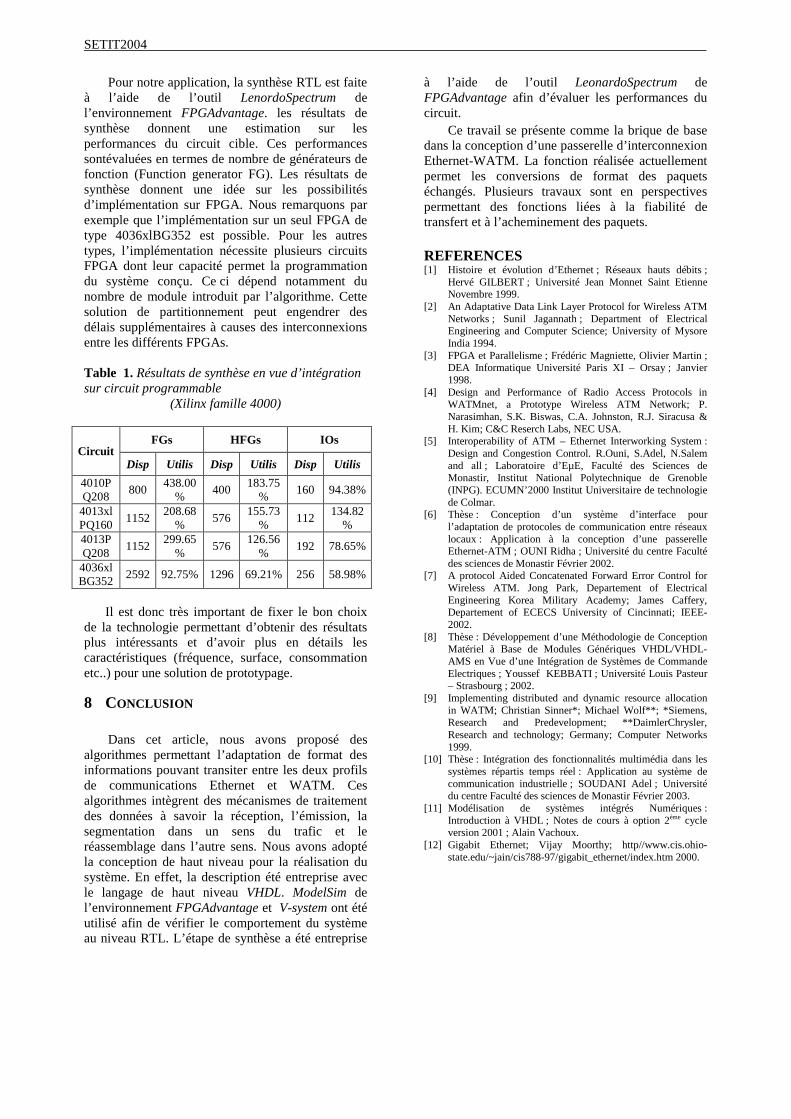
SETIT2004
Pour notre application, la synthèse RTL est faite à l’aide de l’outil LenordoSpectrum de l’environnement FPGAdvantage. les résultats de synthèse donnent une estimation sur les performances du circuit cible. Ces performances sontévaluées en termes de nombre de générateurs de fonction (Function generator FG). Les résultats de synthèse donnent une idée sur les possibilités d’implémentation sur FPGA. Nous remarquons par exemple que l’implémentation sur un seul FPGA de type 4036xlBG352 est possible. Pour les autres types, l’implémentation nécessite plusieurs circuits FPGA dont leur capacité permet la programmation du système conçu. Ce ci dépend notamment du nombre de module introduit par l’algorithme. Cette solution de partitionnement peut engendrer des délais supplémentaires à causes des interconnexions entre les différents FPGAs. Table 1. Résultats de synthèse en vue d’intégration sur circuit programmable
(Xilinx famille 4000)
FGs HFGs IOs Circuit
Disp Utilis Disp Utilis Disp Utilis 4010PQ208 800 438.00
% 400 183.75% 160 94.38%
4013xlPQ160 1152 208.68
% 576 155.73% 112 134.82
% 4013PQ208 1152 299.65
% 576 126.56% 192 78.65%
4036xlBG352 2592 92.75% 1296 69.21% 256 58.98%
Il est donc très important de fixer le bon choix
de la technologie permettant d’obtenir des résultats plus intéressants et d’avoir plus en détails les caractéristiques (fréquence, surface, consommation etc..) pour une solution de prototypage.
8 CONCLUSION
Dans cet article, nous avons proposé des algorithmes permettant l’adaptation de format des informations pouvant transiter entre les deux profils de communications Ethernet et WATM. Ces algorithmes intègrent des mécanismes de traitement des données à savoir la réception, l’émission, la segmentation dans un sens du trafic et le réassemblage dans l’autre sens. Nous avons adopté la conception de haut niveau pour la réalisation du système. En effet, la description été entreprise avec le langage de haut niveau VHDL. ModelSim de l’environnement FPGAdvantage et V-system ont été utilisé afin de vérifier le comportement du système au niveau RTL. L’étape de synthèse a été entreprise
à l’aide de l’outil LeonardoSpectrum de FPGAdvantage afin d’évaluer les performances du circuit.
Ce travail se présente comme la brique de base dans la conception d’une passerelle d’interconnexion Ethernet-WATM. La fonction réalisée actuellement permet les conversions de format des paquets échangés. Plusieurs travaux sont en perspectives permettant des fonctions liées à la fiabilité de transfert et à l’acheminement des paquets.
REFERENCES [1] Histoire et évolution d’Ethernet ; Réseaux hauts débits ;
Hervé GILBERT ; Université Jean Monnet Saint Etienne Novembre 1999.
[2] An Adaptative Data Link Layer Protocol for Wireless ATM Networks ; Sunil Jagannath ; Department of Electrical Engineering and Computer Science; University of Mysore India 1994.
[3] FPGA et Parallelisme ; Frédéric Magniette, Olivier Martin ; DEA Informatique Université Paris XI – Orsay ; Janvier 1998.
[4] Design and Performance of Radio Access Protocols in WATMnet, a Prototype Wireless ATM Network; P. Narasimhan, S.K. Biswas, C.A. Johnston, R.J. Siracusa & H. Kim; C&C Reserch Labs, NEC USA.
[5] Interoperability of ATM – Ethernet Interworking System : Design and Congestion Control. R.Ouni, S.Adel, N.Salem and all ; Laboratoire d’EµE, Faculté des Sciences de Monastir, Institut National Polytechnique de Grenoble (INPG). ECUMN’2000 Institut Universitaire de technologie de Colmar.
[6] Thèse : Conception d’un système d’interface pour l’adaptation de protocoles de communication entre réseaux locaux : Application à la conception d’une passerelle Ethernet-ATM ; OUNI Ridha ; Université du centre Faculté des sciences de Monastir Février 2002.
[7] A protocol Aided Concatenated Forward Error Control for Wireless ATM. Jong Park, Departement of Electrical Engineering Korea Military Academy; James Caffery, Departement of ECECS University of Cincinnati; IEEE-2002.
[8] Thèse : Développement d’une Méthodologie de Conception Matériel à Base de Modules Génériques VHDL/VHDL-AMS en Vue d’une Intégration de Systèmes de Commande Electriques ; Youssef KEBBATI ; Université Louis Pasteur – Strasbourg ; 2002.
[9] Implementing distributed and dynamic resource allocation in WATM; Christian Sinner*; Michael Wolf**; *Siemens, Research and Predevelopment; **DaimlerChrysler, Research and technology; Germany; Computer Networks 1999.
[10] Thèse : Intégration des fonctionnalités multimédia dans les systèmes répartis temps réel : Application au système de communication industrielle ; SOUDANI Adel ; Université du centre Faculté des sciences de Monastir Février 2003.
[11] Modélisation de systèmes intégrés Numériques : Introduction à VHDL ; Notes de cours à option 2ème cycle version 2001 ; Alain Vachoux.
[12] Gigabit Ethernet; Vijay Moorthy; http//www.cis.ohio-state.edu/~jain/cis788-97/gigabit_ethernet/index.htm 2000.
Improvements of the ABR loop performances in a wireless ATM network
Jamila BHAR, Ridha OUNI, Abdelhamid HELALI, Salem NASRI Electronic and Micro-Electronic (EµE) Laboratory,
Faculty of Sciences of Monastir, Tunisia {jamilabhar; ridha_ouni}@yahoo.fr
Abstract There were a number of research activities to promote multimedia and wireless applications rate. Efficient flow and congestion control mechanisms are needed in high-speed networks to meat the new constraints and to offer best quality of service. Mechanisms founded on the rate adjustment had a particular interest. Wireless ATM technology, based on a number of wired ATM protocols and services, is considered a solution for these requirements. It provides multimedia services to mobile users and promises a support of quality of service (QoS). Otherwise, the WATM performances depend on the adopted mechanisms for flow and congestion control. So, several factors can influence this mechanism such as error probability on the wireless link and Handover procedure type. The ABR service, standardized by the ATM forum, is the most widespread traffic congestion control mechanism permitting to provide fair sharing resources. ABR specifications were designed to enable efficient bandwidth allocation and low cell loss ratio. This paper addresses the interaction among the flow control algorithm, the Handover procedure, and the resulting QoS characteristics. We present a novel ABR congestion control algorithm which is adaptive to changing network conditions and robust to terminal mobility. The objective of this algorithm is to achieve a high utilization factor and to maintain the compatibility between the wired and wireless link constraints. Therefore, it was important to develop the necessary mobility enhancements, such as handovers and radio resource management. This approach guarantees the development of an effective control strategy for the congestion control mechanism. Keywords Wireless ATM, ABR, Handover, QoS 1. Introduction The goal of the ABR congestion control mechanism is to fairly share the bandwidth, left over from high priority services, by the ABR connections and to minimize cell loss ratio. The ABR service developed for ATM network cannot be the same used in the wireless ATM environment for various reasons. Indeed, there are supplementary
constraints such as the difficulty to predict the traffic characteristics for mobile terminals, bandwidth loss caused by the supplementary fields in the header, interference phenomenon and important bit error rate on a wireless channel. For these reasons and to provide uniformity of end-to-end quality of service (QoS) guarantees by wireless ATM, it is necessary to focus on the improvement of the existing ABR flow-control algorithms performances. In this paper, we present a robust adaptive congestion control algorithm for ABR service in Wireless ATM networks. The principal design objective was to show that this algorithm performs better with various criteria related to ABR loop characteristics and Handover procedure decision. We consider wireless ATM network environment. The underlying WATM architecture of our study is derived from WAND project prototype [10]. We specify the ABR service class. The flow-control algorithm is specified with two control loops spanning the links between a mobile terminal and its adjacent base station as well as the latter and a data source. We study the impact of handover schemes on this algorithm. Handoff procedure must be capable of dynamically reestablishing virtual circuits to new base stations (BSs) while ensuring minimal loss of data. This paper proceeds as follows. The first section presents the general implementation of ABR flow-control algorithms in a Wireless ATM network. The WATM protocol architecture is also proposed. The next section deals with different types of handovers proposed in the literature, and gives handover solution to support ABR loop performances. The last section shows and evaluates simulation results. Conclusions are stated and issues for future research are discussed. 2. ABR flow-control in a Wireless ATM
network The network supervises without interruption the traffic and provides the feedbacks for the source terminal system. There are many rate-based congestion schemes. ERICA is used as the well-known algorithm [5]. For an ABR connection, information carried in ABR Resource
0-7803-8656-6/04/$20.00 ©2004 IEEE
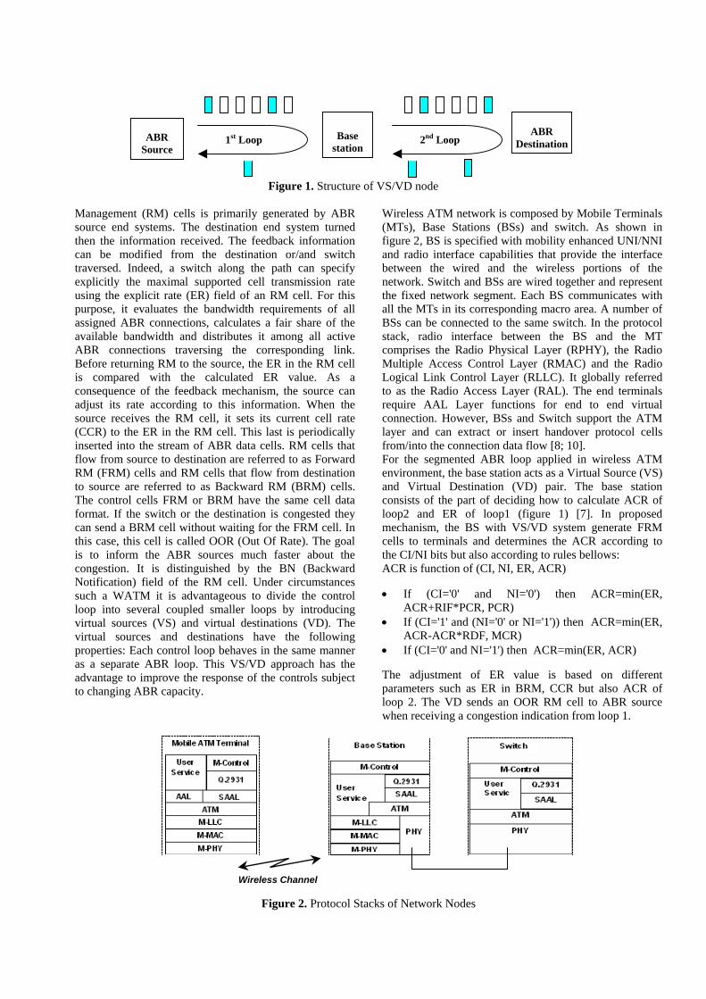
Figure 1. Structure of VS/VD node
Management (RM) cells is primarily generated by ABR source end systems. The destination end system turned then the information received. The feedback information can be modified from the destination or/and switch traversed. Indeed, a switch along the path can specify explicitly the maximal supported cell transmission rate using the explicit rate (ER) field of an RM cell. For this purpose, it evaluates the bandwidth requirements of all assigned ABR connections, calculates a fair share of the available bandwidth and distributes it among all active ABR connections traversing the corresponding link. Before returning RM to the source, the ER in the RM cell is compared with the calculated ER value. As a consequence of the feedback mechanism, the source can adjust its rate according to this information. When the source receives the RM cell, it sets its current cell rate (CCR) to the ER in the RM cell. This last is periodically inserted into the stream of ABR data cells. RM cells that flow from source to destination are referred to as Forward RM (FRM) cells and RM cells that flow from destination to source are referred to as Backward RM (BRM) cells. The control cells FRM or BRM have the same cell data format. If the switch or the destination is congested they can send a BRM cell without waiting for the FRM cell. In this case, this cell is called OOR (Out Of Rate). The goal is to inform the ABR sources much faster about the congestion. It is distinguished by the BN (Backward Notification) field of the RM cell. Under circumstances such a WATM it is advantageous to divide the control loop into several coupled smaller loops by introducing virtual sources (VS) and virtual destinations (VD). The virtual sources and destinations have the following properties: Each control loop behaves in the same manner as a separate ABR loop. This VS/VD approach has the advantage to improve the response of the controls subject to changing ABR capacity.
Wireless ATM network is composed by Mobile Terminals (MTs), Base Stations (BSs) and switch. As shown in figure 2, BS is specified with mobility enhanced UNI/NNI and radio interface capabilities that provide the interface between the wired and the wireless portions of the network. Switch and BSs are wired together and represent the fixed network segment. Each BS communicates with all the MTs in its corresponding macro area. A number of BSs can be connected to the same switch. In the protocol stack, radio interface between the BS and the MT comprises the Radio Physical Layer (RPHY), the Radio Multiple Access Control Layer (RMAC) and the Radio Logical Link Control Layer (RLLC). It globally referred to as the Radio Access Layer (RAL). The end terminals require AAL Layer functions for end to end virtual connection. However, BSs and Switch support the ATM layer and can extract or insert handover protocol cells from/into the connection data flow [8; 10]. For the segmented ABR loop applied in wireless ATM environment, the base station acts as a Virtual Source (VS) and Virtual Destination (VD) pair. The base station consists of the part of deciding how to calculate ACR of loop2 and ER of loop1 (figure 1) [7]. In proposed mechanism, the BS with VS/VD system generate FRM cells to terminals and determines the ACR according to the CI/NI bits but also according to rules bellows: ACR is function of (CI, NI, ER, ACR) • If (CI='0' and NI='0') then ACR=min(ER,
ACR+RIF*PCR, PCR) • If (CI='1' and (NI='0' or NI='1')) then ACR=min(ER,
ACR-ACR*RDF, MCR) • If (CI='0' and NI='1') then ACR=min(ER, ACR) The adjustment of ER value is based on different parameters such as ER in BRM, CCR but also ACR of loop 2. The VD sends an OOR RM cell to ABR source when receiving a congestion indication from loop 1.
Figure 2. Protocol Stacks of Network Nodes
Wireless Channel
ABR
Source Base
station
ABR
Destination 1st Loop 2nd Loop
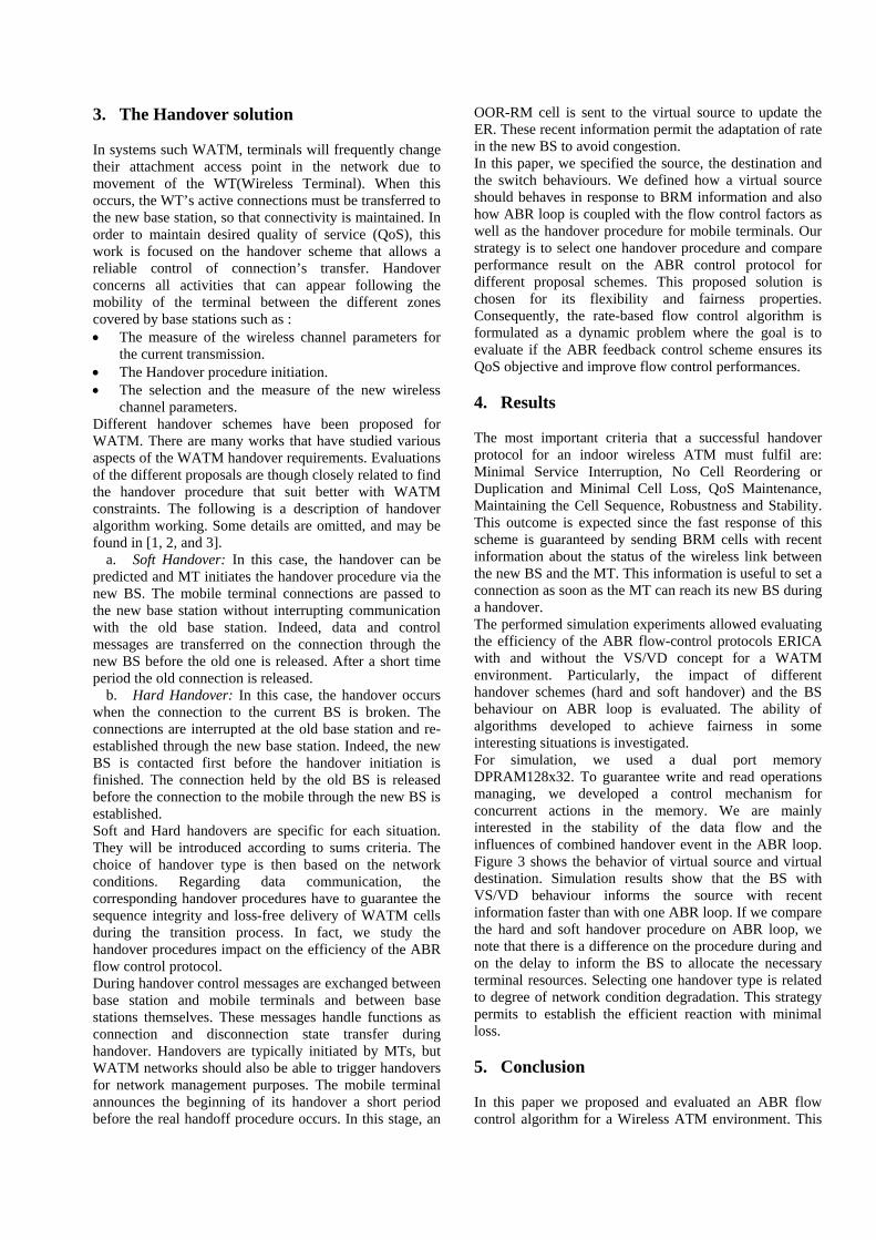
3. The Handover solution In systems such WATM, terminals will frequently change their attachment access point in the network due to movement of the WT(Wireless Terminal). When this occurs, the WT’s active connections must be transferred to the new base station, so that connectivity is maintained. In order to maintain desired quality of service (QoS), this work is focused on the handover scheme that allows a reliable control of connection’s transfer. Handover concerns all activities that can appear following the mobility of the terminal between the different zones covered by base stations such as : • The measure of the wireless channel parameters for
the current transmission. • The Handover procedure initiation. • The selection and the measure of the new wireless
channel parameters. Different handover schemes have been proposed for WATM. There are many works that have studied various aspects of the WATM handover requirements. Evaluations of the different proposals are though closely related to find the handover procedure that suit better with WATM constraints. The following is a description of handover algorithm working. Some details are omitted, and may be found in [1, 2, and 3].
a. Soft Handover: In this case, the handover can be predicted and MT initiates the handover procedure via the new BS. The mobile terminal connections are passed to the new base station without interrupting communication with the old base station. Indeed, data and control messages are transferred on the connection through the new BS before the old one is released. After a short time period the old connection is released.
b. Hard Handover: In this case, the handover occurs when the connection to the current BS is broken. The connections are interrupted at the old base station and re-established through the new base station. Indeed, the new BS is contacted first before the handover initiation is finished. The connection held by the old BS is released before the connection to the mobile through the new BS is established. Soft and Hard handovers are specific for each situation. They will be introduced according to sums criteria. The choice of handover type is then based on the network conditions. Regarding data communication, the corresponding handover procedures have to guarantee the sequence integrity and loss-free delivery of WATM cells during the transition process. In fact, we study the handover procedures impact on the efficiency of the ABR flow control protocol. During handover control messages are exchanged between base station and mobile terminals and between base stations themselves. These messages handle functions as connection and disconnection state transfer during handover. Handovers are typically initiated by MTs, but WATM networks should also be able to trigger handovers for network management purposes. The mobile terminal announces the beginning of its handover a short period before the real handoff procedure occurs. In this stage, an
OOR-RM cell is sent to the virtual source to update the ER. These recent information permit the adaptation of rate in the new BS to avoid congestion. In this paper, we specified the source, the destination and the switch behaviours. We defined how a virtual source should behaves in response to BRM information and also how ABR loop is coupled with the flow control factors as well as the handover procedure for mobile terminals. Our strategy is to select one handover procedure and compare performance result on the ABR control protocol for different proposal schemes. This proposed solution is chosen for its flexibility and fairness properties. Consequently, the rate-based flow control algorithm is formulated as a dynamic problem where the goal is to evaluate if the ABR feedback control scheme ensures its QoS objective and improve flow control performances. 4. Results The most important criteria that a successful handover protocol for an indoor wireless ATM must fulfil are: Minimal Service Interruption, No Cell Reordering or Duplication and Minimal Cell Loss, QoS Maintenance, Maintaining the Cell Sequence, Robustness and Stability. This outcome is expected since the fast response of this scheme is guaranteed by sending BRM cells with recent information about the status of the wireless link between the new BS and the MT. This information is useful to set a connection as soon as the MT can reach its new BS during a handover. The performed simulation experiments allowed evaluating the efficiency of the ABR flow-control protocols ERICA with and without the VS/VD concept for a WATM environment. Particularly, the impact of different handover schemes (hard and soft handover) and the BS behaviour on ABR loop is evaluated. The ability of algorithms developed to achieve fairness in some interesting situations is investigated. For simulation, we used a dual port memory DPRAM128x32. To guarantee write and read operations managing, we developed a control mechanism for concurrent actions in the memory. We are mainly interested in the stability of the data flow and the influences of combined handover event in the ABR loop. Figure 3 shows the behavior of virtual source and virtual destination. Simulation results show that the BS with VS/VD behaviour informs the source with recent information faster than with one ABR loop. If we compare the hard and soft handover procedure on ABR loop, we note that there is a difference on the procedure during and on the delay to inform the BS to allocate the necessary terminal resources. Selecting one handover type is related to degree of network condition degradation. This strategy permits to establish the efficient reaction with minimal loss. 5. Conclusion In this paper we proposed and evaluated an ABR flow control algorithm for a Wireless ATM environment. This
Data cells Reception of FRM cell
Figure 3. VS/VD behavior of BS
algorithm ameliorates the congestion control performances by adding new constraints to the ABR loop. Results obtained justify that it is important to consider suitable handover protocols in order to maintain QoS parameters. The proposed mechanism supports optimum Handover procedure when required. Thus, it minimizes the total execution time of handovers. An additional advantage is focused on the same actions performed during soft and hard handovers. This characteristic facilitates the implementation of the required functional entities. In conclusion, the impact of handover protocols on WATM performances over ABR service class is considerable and provides an alternative approach that requires further studies. The aim of handoff signalling is to enable wireless terminals to move seamlessly between BSs while maintaining connections with their negotiated QoS. For this purpose, there is a close inter-working with the connection management and rerouting functions of the BS. The format of signalling messages exchanged at handover procedure may be also optimised to guarantee Qos requirements. Therefore, the employment of ARQ scheme will reduce the cell loss rate due to the error characteristics of the wireless link. The future work will adopt a rerouting scheme for proposed handoff procedure. The proposed handover mechanism can also be developed to support inter-switch handovers. References [1] Adaptation of the Fuzzy Explicit Rate Marking to ABR flow-control in wireless ATM Netwok; Michael Savoric, Department of Electrical Engineering Technical University of Berlin; Udo R.Krieger, Deutsche Telekom AG Technologiezentrum Am Kavalleriesand Germany. MMB 99, Trier, September 1999. [2] The Impact of Handover Protocols on the performance of ABR flow-Control Algorithms in a Wireless ATM Network; Michael Savoric, Adam Wolisz, Department of Electrical Engineering TU Berlin Germany; Udo R.Krieger, T-Nova Deutsche Telekom, Am Kavalleriesand Germany. European Transactions on Telecommunications (ETT) Journal, July-August 2000.
[3] Performance evaluation of Handover protocols for data communication in a Wireless ATM network; Udo R.Krieger and Michael Savoric; ITC16, Edinburgh, June 1999. [4] ABR Traffic Congestion Control Mechanism with VS/VD in Wireless ATM Networks; Moonsik Kang, Sangmin Lee, Department of Electronic Engineering, Kangnung National University Kangwon Kangnung Korea; 2000. [5] ERICA Switch Algorithm : A Complete Description, ATM Forum/96, Raj Jain, Shiv Kalyanaraman, Rohit Goyal, Sonia Fahmy, Ram Viswanathan; The Ohio State University Department of CIS Columbus; http://www.cis.ohio-state.edu/~jain/ [6] Source Behavior for ATM ABR Traffic Management: An Explanation; Raj Jain, Shivkumar Kalyanaraman, Sonia Fahmy and Rohit Goyal; Department of Computer and Information Science; The Ohio State University; and Seong-Cheol Kim; Samsung Electronics Co. Ltd.Chung-Ang Newspaper Bldg; 1996 [7] Design considerations for the virtual source/virtual destination; VS/VD feature in the ABR service of ATM networks; Shivkumar Kalyanaraman; Raj Jain; Jianping Jiang; Rohit Goyal; Sonia Fahmy; Department of Computer and Information Science, The Ohio State UniÕersity, Columbus, USA; June 1998 [8] Local and Global Handovers Based on In-Band Signaling in Wireless ATM Networks; M.AJMONE MARSAN; C.F.CHIASSERINI; A.FUMAGALLI; R.LO CIGNO and M.MUNAFÒ; Wireless Networks,2001 [9] Microcellular Handover in Wireless ATM; Fan Jiang ; Timo Käkölä; Proceedings of the 32nd Hawaii International Conference on System Sciences – 1999 [10] Implementation of the wireless ATM access terminal; Juha Ala-Laurila; Jussi Lemilainen; Nokia Wireless Business Communications, Computer Networks; 1999.
Data cells memorized
VS
VD
RM cell filtered
Emission of BRM cell
Emission of FRM cell
Reception of BRM cell